Embed Size (px)
Citation preview

INTER-UNIVERSAL TEICHMULLER THEORY IV:
LOG-VOLUME COMPUTATIONS AND
SET-THEORETIC FOUNDATIONS
Shinichi Mochizuki
December 2017
Abstract. The present paper forms the fourth and final paper in a seriesof papers concerning “inter-universal Teichmuller theory”. In the first threepapers of the series, we introduced and studied the theory surrounding the log-
theta-lattice, a highly non-commutative two-dimensional diagram of “miniaturemodels of conventional scheme theory”, called Θ±ellNF-Hodge theaters, that wereassociated, in the first paper of the series, to certain data, called initial Θ-data.
This data includes an elliptic curve EF over a number field F , together with aprime number l ≥ 5. Consideration of various properties of the log-theta-latticeled naturally to the establishment, in the third paper of the series, of multiradialalgorithms for constructing “splitting monoids of LGP-monoids”. Here, we
recall that “multiradial algorithms” are algorithms that make sense from the pointof view of an “alien arithmetic holomorphic structure”, i.e., the ring/schemestructure of a Θ±ellNF-Hodge theater related to a given Θ±ellNF-Hodge theater bymeans of a non-ring/scheme-theoretic horizontal arrow of the log-theta-lattice. In
the present paper, estimates arising from these multiradial algorithms for splittingmonoids of LGP-monoids are applied to verify various diophantine results whichimply, for instance, the so-called Vojta Conjecture for hyperbolic curves, the ABCConjecture, and the Szpiro Conjecture for elliptic curves. Finally, we examine
— albeit from an extremely naive/non-expert point of view! — the foundational/set-theoretic issues surrounding the vertical and horizontal arrows of the log-theta-latticeby introducing and studying the basic properties of the notion of a “species”, whichmay be thought of as a sort of formalization, via set-theoretic formulas, of the intuitive
notion of a “type of mathematical object”. These foundational issues are closelyrelated to the central role played in the present series of papers by various resultsfrom absolute anabelian geometry, as well as to the idea of gluing together
distinct models of conventional scheme theory, i.e., in a fashion that lies outside theframework of conventional scheme theory. Moreover, it is precisely these foundationalissues surrounding the vertical and horizontal arrows of the log-theta-lattice that lednaturally to the introduction of the term “inter-universal”.
Contents:
Introduction§0. Notations and Conventions§1. Log-volume Estimates§2. Diophantine Inequalities§3. Inter-universal Formalism: the Language of Species
Typeset by AMS-TEX1

2 SHINICHI MOCHIZUKI
Introduction
The present paper forms the fourth and final paper in a series of papers concern-ing “inter-universal Teichmuller theory”. In the first three papers, [IUTchI],[IUTchII], and [IUTchIII], of the series, we introduced and studied the theory sur-rounding the log-theta-lattice [cf. the discussion of [IUTchIII], Introduction],a highly non-commutative two-dimensional diagram of “miniature models of con-ventional scheme theory”, called Θ±ellNF-Hodge theaters, that were associated, inthe first paper [IUTchI] of the series, to certain data, called initial Θ-data. Thisdata includes an elliptic curve EF over a number field F , together with a primenumber l ≥ 5 [cf. [IUTchI], §I1]. Consideration of various properties of the log-theta-lattice leads naturally to the establishment of multiradial algorithms forconstructing “splitting monoids of LGP-monoids” [cf. [IUTchIII], TheoremA]. Here, we recall that “multiradial algorithms” [cf. the discussion of the Intro-ductions to [IUTchII], [IUTchIII]] are algorithms that make sense from the pointof view of an “alien arithmetic holomorphic structure”, i.e., the ring/schemestructure of a Θ±ellNF-Hodge theater related to a given Θ±ellNF-Hodge theater bymeans of a non-ring/scheme-theoretic horizontal arrow of the log-theta-lattice. Inthe final portion of [IUTchIII], by applying these multiradial algorithms for split-ting monoids of LGP-monoids, we obtained estimates for the log-volume of theseLGP-monoids [cf. [IUTchIII], Theorem B]. In the present paper, these estimateswill be applied to verify various diophantine results.
In §1 of the present paper, we start by discussing various elementary estimatesfor the log-volume of various tensor products of the modules obtained by applyingthe p-adic logarithm to the local units — i.e., in the terminology of [IUTchIII],“tensor packets of log-shells” [cf. the discussion of [IUTchIII], Introduction] — interms of various well-known invariants, such as differents, associated to a mixed-characteristic nonarchimedean local field [cf. Propositions 1.1, 1.2, 1.3, 1.4]. Wethen discuss similar — but technically much simpler! — log-volume estimates inthe case of complex archimedean local fields [cf. Proposition 1.5]. After review-ing a certain classical estimate concerning the distribution of prime numbers [cf.Proposition 1.6], as well as some elementary general nonsense concerning weightedaverages [cf. Proposition 1.7] and well-known elementary facts concerning ellipticcurves [cf. Proposition 1.8], we then proceed to compute explicitly, in more elemen-tary language, the quantity that was estimated in [IUTchIII], Theorem B. Thesecomputations yield a quite strong/explicit diophantine inequality [cf. Theorem1.10] concerning elliptic curves that are in “sufficiently general position”, sothat one may apply the general theory developed in the first three papers of theseries.
In §2 of the present paper, after reviewing another classical estimate concern-ing the distribution of prime numbers [cf. Proposition 2.1, (ii)], we then proceedto apply the theory of [GenEll] to reduce various diophantine results concerningan arbitrary elliptic curve over a number field to results of the type obtained inTheorem 1.10 concerning elliptic curves that are in “sufficiently general posi-tion” [cf. Corollary 2.2]. This reduction allows us to derive the following result[cf. Corollary 2.3], which constitutes the main application of the “inter-universalTeichmuller theory” developed in the present series of papers.
INTER-UNIVERSAL TEICHMULLER THEORY IV 3
Theorem A. (Diophantine Inequalities) Let X be a smooth, proper, geomet-
rically connected curve over a number field; D ⊆ X a reduced divisor; UXdef= X\D;
d a positive integer; ε ∈ R>0 a positive real number. Write ωX for the canon-ical sheaf on X. Suppose that UX is a hyperbolic curve, i.e., that the degreeof the line bundle ωX(D) is positive. Then, relative to the notation of [GenEll][reviewed in the discussion preceding Corollary 2.2 of the present paper], one hasan inequality of “bounded discrepancy classes”
htωX(D) � (1 + ε)(log-diffX + log-condD)
of functions on UX(Q)≤d — i.e., the function (1 + ε)(log-diffX + log-condD) −htωX(D) is bounded below by a constant on UX(Q)≤d [cf. [GenEll], Definition 1.2,(ii), as well as Remark 2.3.1, (ii), of the present paper].
Thus, Theorem A asserts an inequality concerning the canonical height [i.e.,“htωX(D)”], the logarithmic different [i.e., “log-diffX”], and the logarithmic conduc-tor [i.e., “log-condD”] of points of the curve UX valued in number fields whoseextension degree over Q is ≤ d . In particular, the so-called Vojta Conjecture forhyperbolic curves, the ABC Conjecture, and the Szpiro Conjecture for ellipticcurves all follow as special cases of Theorem A. We refer to [Vjt] for a detailedexposition of these conjectures.
Finally, in §3, we examine — albeit from an extremely naive/non-expert pointof view! — certain foundational issues underlying the theory of the present se-ries of papers. Typically in mathematical discussions [i.e., by mathematicians whoare not equipped with a detailed knowledge of the theory of foundations!] — suchas, for instance, the theory developed in the present series of papers! — one de-fines various “types of mathematical objects” [i.e., such as groups, topologicalspaces, or schemes], together with a notion of “morphisms” between two partic-ular examples of a specific type of mathematical object [i.e., morphisms betweengroups, between topological spaces, or between schemes]. Such objects and mor-phisms [typically] determine a category. On the other hand, if one restricts one’sattention to such a category, then one must keep in mind the fact that the structureof the category — i.e., which consists only of a collection of objects and morphismssatisfying certain properties! — does not include any mention of the various setsand conditions satisfied by those sets that give rise to the “type of mathematicalobject” under consideration. For instance, the data consisting of the underlyingset of a group, the group multiplication law on the group, and the properties sat-isfied by this group multiplication law cannot be recovered [at least in an a priorisense!] from the structure of the “category of groups”. Put another way, althoughthe notion of a “type of mathematical object” may give rise to a “category of suchobjects”, the notion of a “type of mathematical object” is much stronger — in thesense that it involves much more mathematical structure — than the notion of a cat-egory. Indeed, a given “type of mathematical object” may have a very complicatedinternal structure, but may give rise to a category equivalent to a one-morphismcategory [i.e., a category with precisely one morphism]; in particular, in such cases,the structure of the associated category does not retain any information of inter-est concerning the internal structure of the “type of mathematical object” underconsideration.
4 SHINICHI MOCHIZUKI
In Definition 3.1, (iii), we formalize this intuitive notion of a “type of mathe-matical object” by defining the notion of a species as, roughly speaking, a collectionof set-theoretic formulas that gives rise to a category in any given model of set the-ory [cf. Definition 3.1, (iv)], but, unlike any specific category [e.g., of groups, etc.] isnot confined to any specific model of set theory. In a similar vein, by workingwith collections of set-theoretic formulas, one may define a species-theoretic ana-logue of the notion of a functor, which we refer to as a mutation [cf. Definition 3.3,(i)]. Given a diagram of mutations, one may then define the notion of a “mutationthat extracts, from the diagram, a certain portion of the types of mathematicalobjects that appear in the diagram that is invariant with respect to the mutationsin the diagram”; we refer to such a mutation as a core [cf. Definition 3.3, (v)].
One fundamental example, in the context of the present series of papers, of adiagram of mutations is the usual set-up of [absolute] anabelian geometry [cf.Example 3.5 for more details]. That is to say, one begins with the species constitutedby schemes satisfying certain conditions. One then considers the mutation
X � ΠX
that associates to such a scheme X its etale fundamental group ΠX [say, consideredup to inner automorphisms]. Here, it is important to note that the codomain ofthis mutation is the species constituted by topological groups [say, considered upto inner automorphisms] that satisfy certain conditions which do not include anyinformation concerning how the group is related [for instance, via some sort ofetale fundamental group mutation] to a scheme. The notion of an anabelianreconstruction algorithm may then be formalized as a mutation that forms a“mutation-quasi-inverse” to the fundamental group mutation.
Another fundamental example, in the context of the present series of papers, ofa diagram of mutations arises from the Frobenius morphism in positive characteristicscheme theory [cf. Example 3.6 for more details]. That is to say, one fixes a primenumber p and considers the species constituted by reduced quasi-compact schemesof characteristic p and quasi-compact morphisms of schemes. One then considersthe mutation that associates
S � S(p)
to such a scheme S the scheme S(p) with the same topological space, but whoseregular functions are given by the p-th powers of the regular functions on the originalscheme. Thus, the domain and codomain of this mutation are given by the samespecies. One may also consider a log scheme version of this example, which, at thelevel of monoids, corresponds, in essence, to assigning
M � p ·Mto a torsion-free abelian monoid M the submonoid p ·M ⊆ M determined by theimage of multiplication by p. Returning to the case of schemes, one may thenobserve that the well-known constructions of the perfection and the etale site
S � Spf; S � Set
associated to a reduced scheme S of characteristic p give rise to cores of the diagramobtained by considering iterates of the “Frobenius mutation” just discussed.
INTER-UNIVERSAL TEICHMULLER THEORY IV 5
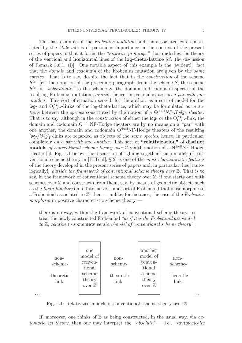
This last example of the Frobenius mutation and the associated core consti-tuted by the etale site is of particular importance in the context of the presentseries of papers in that it forms the “intuitive prototype” that underlies the theoryof the vertical and horizontal lines of the log-theta-lattice [cf. the discussionof Remark 3.6.1, (i)]. One notable aspect of this example is the [evident!] factthat the domain and codomain of the Frobenius mutation are given by the samespecies. That is to say, despite the fact that in the construction of the schemeS(p) [cf. the notation of the preceding paragraph] from the scheme S, the schemeS(p) is “subordinate” to the scheme S, the domain and codomain species of theresulting Frobenius mutation coincide, hence, in particular, are on a par with oneanother. This sort of situation served, for the author, as a sort of model for thelog- and Θ×μ
LGP-links of the log-theta-lattice, which may be formulated as muta-tions between the species constituted by the notion of a Θ±ellNF-Hodge theater.That is to say, although in the construction of either the log- or the Θ×μ
LGP-link, thedomain and codomain Θ±ellNF-Hodge theaters are by no means on a “par” withone another, the domain and codomain Θ±ellNF-Hodge theaters of the resultinglog-/Θ×μ
LGP-links are regarded as objects of the same species, hence, in particular,completely on a par with one another. This sort of “relativization” of distinctmodels of conventional scheme theory over Z via the notion of a Θ±ellNF-Hodgetheater [cf. Fig. I.1 below; the discussion of “gluing together” such models of con-ventional scheme theory in [IUTchI], §I2] is one of the most characteristic featuresof the theory developed in the present series of papers and, in particular, lies [tauto-logically!] outside the framework of conventional scheme theory over Z. That is tosay, in the framework of conventional scheme theory over Z, if one starts out withschemes over Z and constructs from them, say, by means of geometric objects suchas the theta function on a Tate curve, some sort of Frobenioid that is isomorphic toa Frobenioid associated to Z, then — unlike, for instance, the case of the Frobeniusmorphism in positive characteristic scheme theory —
there is no way, within the framework of conventional scheme theory, totreat the newly constructed Frobenioid “as if it is the Frobenioid associatedto Z, relative to some new version/model of conventional scheme theory”.
. . .
non-scheme-
—————theoreticlink
onemodel ofconven-tionalschemetheoryover Z
non-scheme-
—————theoreticlink
anothermodel ofconven-tionalschemetheoryover Z
non-scheme-
—————theoreticlink
. . .
Fig. I.1: Relativized models of conventional scheme theory over Z
If, moreover, one thinks of Z as being constructed, in the usual way, via ax-iomatic set theory, then one may interpret the “absolute” — i.e., “tautologically
6 SHINICHI MOCHIZUKI
unrelativizable” — nature of conventional scheme theory over Z at a purely set-theoretic level. Indeed, from the point of view of the “∈-structure” of axiomatic settheory, there is no way to treat sets constructed at distinct levels of this ∈-structureas being on a par with one another. On the other hand, if one focuses not onthe level of the ∈-structure to which a set belongs, but rather on species, then thenotion of a species allows one to relate — i.e., to treat on a par with one another —objects belonging to the species that arise from sets constructed at distinct levelsof the ∈-structure. That is to say,
the notion of a species allows one to “simulate ∈-loops” without vio-lating the axiom of foundation of axiomatic set theory
— cf. the discussion of Remark 3.3.1, (i).
As one constructs sets at new levels of the ∈-structure of some model of ax-iomatic set theory — e.g., as one travels along vertical or horizontal lines of thelog-theta-lattice! — one typically encounters new schemes, which give rise to newGalois categories, hence to new Galois or etale fundamental groups, which mayonly be constructed if one allows oneself to consider new basepoints, relative to newuniverses. In particular, one must continue to extend the universe, i.e., to modifythe model of set theory, relative to which one works. Here, we recall in passingthat such “extensions of universe” are possible on account of an existence axiomconcerning universes, which is apparently attributed to the “Grothendieck school”and, moreover, cannot, apparently, be obtained as a consequence of the conven-tional ZFC axioms of axiomatic set theory [cf. the discussion at the beginning of§3 for more details]. On the other hand, ultimately in the present series of papers[cf. the discussion of [IUTchIII], Introduction], we wish to obtain algorithms forconstructing various objects that arise in the context of the new schemes/universesdiscussed above — i.e., at distant Θ±ellNF-Hodge theaters of the log-theta-lattice— that make sense from the point of view of the original schemes/universes thatoccurred at the outset of the discussion. Again, the fundamental tool that makesthis possible, i.e., that allows one to express constructions in the new universes interms that makes sense in the original universe is precisely
the species-theoretic formulation — i.e., the formulation via set-theoretic formulas that do not depend on particular choices invokedin particular universes — of the constructions of interest
— cf. the discussion of Remarks 3.1.2, 3.1.3, 3.1.4, 3.1.5, 3.6.2, 3.6.3. This isthe point of view that gave rise to the term “inter-universal”. At a more con-crete level, this “inter-universal” contact between constructions in distant modelsof conventional scheme theory in the log-theta-lattice is realized by considering [theetale-like structures given by] the various Galois or etale fundamental groups thatoccur as [the “type of mathematical object”, i.e., species constituted by] abstracttopological groups [cf. the discussion of Remark 3.6.3, (i); [IUTchI], §I3]. Theseabstract topological groups give rise to vertical or horizontal cores of the log-theta-lattice [cf. the discussion of [IUTchIII], Introduction; [IUTchIII], Theorem1.5, (i), (ii)]. Moreover, once one obtains cores that are sufficiently “nondegener-ate”, or “rich in structure”, so as to serve as containers for the non-coric portions of
INTER-UNIVERSAL TEICHMULLER THEORY IV 7
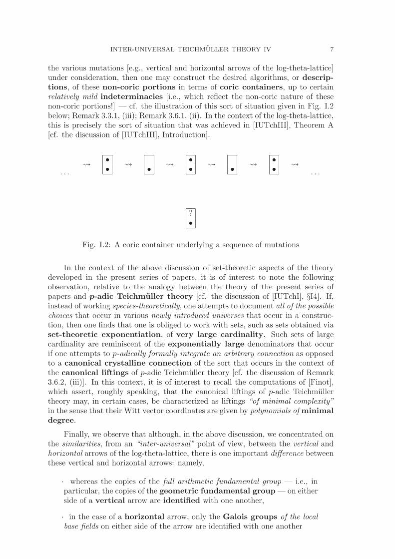
the various mutations [e.g., vertical and horizontal arrows of the log-theta-lattice]under consideration, then one may construct the desired algorithms, or descrip-tions, of these non-coric portions in terms of coric containers, up to certainrelatively mild indeterminacies [i.e., which reflect the non-coric nature of thesenon-coric portions!] — cf. the illustration of this sort of situation given in Fig. I.2below; Remark 3.3.1, (iii); Remark 3.6.1, (ii). In the context of the log-theta-lattice,this is precisely the sort of situation that was achieved in [IUTchIII], Theorem A[cf. the discussion of [IUTchIII], Introduction].
. . .� •
• � • � •• � • � •
• �. . .
?•
Fig. I.2: A coric container underlying a sequence of mutations
In the context of the above discussion of set-theoretic aspects of the theorydeveloped in the present series of papers, it is of interest to note the followingobservation, relative to the analogy between the theory of the present series ofpapers and p-adic Teichmuller theory [cf. the discussion of [IUTchI], §I4]. If,instead of working species-theoretically, one attempts to document all of the possiblechoices that occur in various newly introduced universes that occur in a construc-tion, then one finds that one is obliged to work with sets, such as sets obtained viaset-theoretic exponentiation, of very large cardinality. Such sets of largecardinality are reminiscent of the exponentially large denominators that occurif one attempts to p-adically formally integrate an arbitrary connection as opposedto a canonical crystalline connection of the sort that occurs in the context ofthe canonical liftings of p-adic Teichmuller theory [cf. the discussion of Remark3.6.2, (iii)]. In this context, it is of interest to recall the computations of [Finot],which assert, roughly speaking, that the canonical liftings of p-adic Teichmullertheory may, in certain cases, be characterized as liftings “of minimal complexity”in the sense that their Witt vector coordinates are given by polynomials of minimaldegree.
Finally, we observe that although, in the above discussion, we concentrated onthe similarities, from an “inter-universal” point of view, between the vertical andhorizontal arrows of the log-theta-lattice, there is one important difference betweenthese vertical and horizontal arrows: namely,
· whereas the copies of the full arithmetic fundamental group — i.e., inparticular, the copies of the geometric fundamental group — on eitherside of a vertical arrow are identified with one another,
· in the case of a horizontal arrow, only the Galois groups of the localbase fields on either side of the arrow are identified with one another
8 SHINICHI MOCHIZUKI
— cf. the discussion of Remark 3.6.3, (ii). One way to understand the reasonfor this difference is as follows. In the case of the vertical arrows — i.e., the log-links, which, in essence, amount to the various local p-adic logarithms — in orderto construct the log-link, it is necessary to make use, in an essential way, of thelocal ring structures at v ∈ V [cf. the discussion of [IUTchIII], Definition 1.1,(i), (ii)], which may only be reconstructed from the full arithmetic fundamental
group. By contrast, in order to construct the horizontal arrows — i.e., the Θ×μLGP-
links — this local ring structure is unnecessary. On the other hand, in order toconstruct the horizontal arrows, it is necessary to work with structures that, upto isomorphism, are common to both the domain and the codomain of the arrow.Since the construction of the domain of the Θ×μ
LGP-link depends, in an essential
way, on the Gaussian monoids, i.e., on the labels ∈ F�l for the theta values,
which are constructed from the geometric fundamental group, while the codomainonly involves monoids arising from the local q-parameters “q
v” [for v ∈ V
bad], which
are constructed in a fashion that is independent of these labels, in order to obtainan isomorphism between structures arising from the domain and codomain, it isnecessary to restrict one’s attention to the Galois groups of the local base fields,which are free of any dependence on these labels.
Acknowledgements:
The research discussed in the present paper profited enormously from the gen-erous support that the author received from the Research Institute for MathematicalSciences, a Joint Usage/Research Center located in Kyoto University. At a personallevel, I would like to thank Fumiharu Kato, Akio Tamagawa, Go Yamashita, Mo-hamed Saıdi, Yuichiro Hoshi, Ivan Fesenko, Fucheng Tan, and Emmanuel Lepagefor many stimulating discussions concerning the material presented in this paper.Also, I feel deeply indebted to Go Yamashita, Mohamed Saıdi, and Yuichiro Hoshifor their meticulous reading of and numerous comments concerning the presentpaper. In addition, I would like to thank Kentaro Sato for useful comments con-cerning the set-theoretic and foundational aspects of the present paper, as well asVesselin Dimitrov and Akshay Venkatesh for useful comments concerning the ana-lytic number theory aspects of the present paper. Finally, I would like to expressmy deep gratitude to Ivan Fesenko for his quite substantial efforts to disseminate— for instance, in the form of a survey that he wrote — the theory discussed inthe present series of papers.
Notations and Conventions:
We shall continue to use the “Notations and Conventions” of [IUTchI], §0.

INTER-UNIVERSAL TEICHMULLER THEORY IV 9
Section 1: Log-volume Estimates
In the present §1, we perform various elementary local computations con-cerning nonarchimedean and archimedean local fields which allow us to obtainmoreexplicit versions [cf. Theorem 1.10 below] of the log-volume estimates for Θ-pilot objects obtained in [IUTchIII], Corollary 3.12.
In the following, if λ ∈ R, then we shall write
�λ� (respectively, �λ)
for the smallest (respectively, largest) n ∈ Z such that n ≥ λ (respectively, n ≤ λ).Also, we shall write “log(−)” for the natural logarithm of a positive real number.
Proposition 1.1. (Multiple Tensor Products and Differents) Let p bea prime number, I a finite set of cardinality ≥ 2, Qp an algebraic closure of Qp.
Write R ⊆ Qp for the ring of integers of Qp and ord : Q×p → Q for the natural
p-adic valuation on Qp, normalized so that ord(p) = 1; for λ ∈ Q, we shall write
pλ for “some” [unspecified] element of Qp such that ord(pλ) = λ. For i ∈ I, let
ki ⊆ Qp be a finite extension of Qp; write Ridef= Oki
= R⋂ki for the ring of
integers of ki and di ∈ Q≥0 for the order [i.e., “ord(−)”] of any generator of thedifferent ideal of Ri over Zp. Also, for any nonempty subset E ⊆ I, let us write
REdef=
⊗i∈E
Ri; dEdef=
∑i∈E
di
— where the tensor product is over Zp. Fix an element ∗ ∈ I; write I∗ def= I \ {∗}.
ThenpdI∗ · (RI)
∼ ⊆ RI ⊆ (RI)∼
— where we write “(−)∼” for the normalization of the [reduced] ring in paren-theses in its ring of fractions, and we observe that it follows immediately from thedefinition of the “normalization” that the notation on the left-hand side of the firstinclusion of the above display is well-defined for suitable “pdI∗” [such as productsof elements pdi ∈ Ri, for i ∈ I∗] and independent of the choice of such suitable“pdI∗”.
Proof. Let us regard RI as an R∗-algebra in the evident fashion. It is immediatefrom the definitions that RI ⊆ (RI)
∼. Now observe that
R⊗R∗ RI ⊆ R⊗R∗ (RI)∼ ⊆ (R⊗R∗ RI)
∼
— where (R⊗R∗ RI)∼ decomposes as a direct sum of finitely many copies of R. In
particular, one verifies immediately, in light of the fact the R is faithfully flat overR∗, that to complete the proof of Proposition 1.1, it suffices to verify that
pdI∗ · (R⊗R∗ RI)∼ ⊆ R⊗R∗ RI
10 SHINICHI MOCHIZUKI
— where we observe that it follows immediately from the definition of the “nor-malization” that the notation on the left-hand side of the inclusion of the abovedisplay is well-defined and independent of the choice of “pdI∗”. On the other hand,it follows immediately from induction on the cardinality of I that to verify this lastinclusion, it suffices to verify the inclusion in the case where I is of cardinality two.But in this case, the desired inclusion follows immediately from the definition ofthe different ideal. This completes the proof of Proposition 1.1. ©
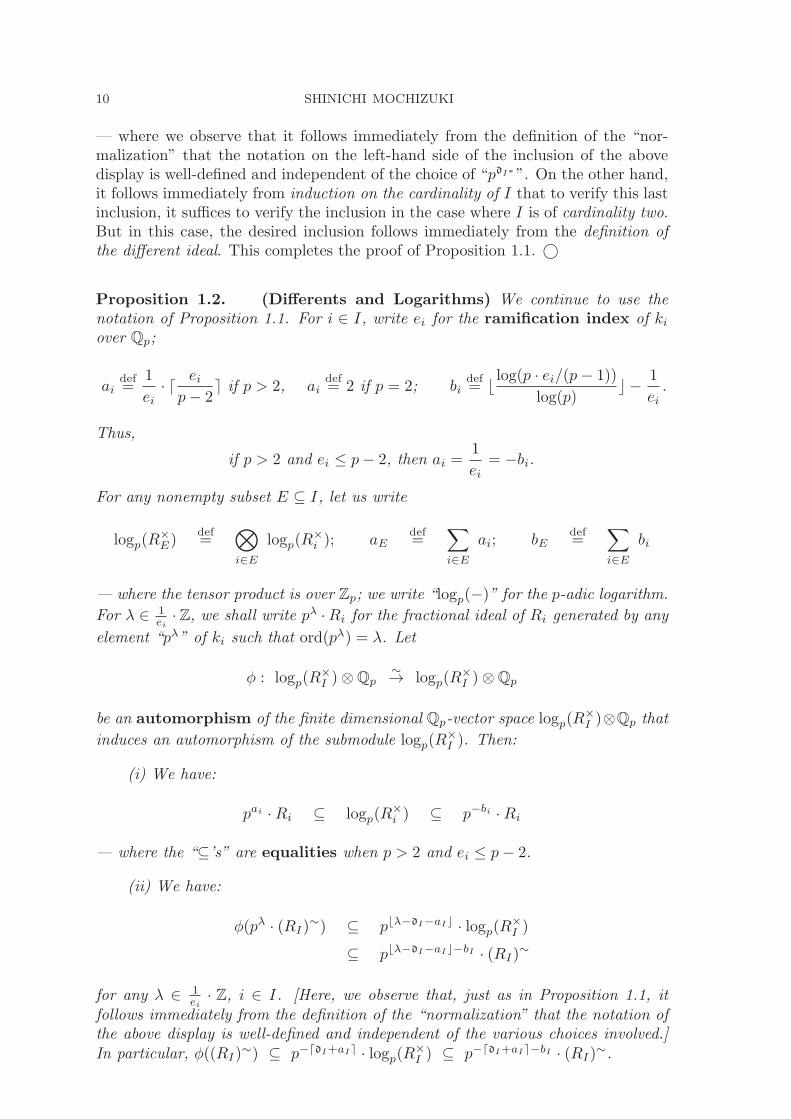
Proposition 1.2. (Differents and Logarithms) We continue to use thenotation of Proposition 1.1. For i ∈ I, write ei for the ramification index of kiover Qp;
aidef=
1
ei· � ei
p− 2� if p > 2, ai
def= 2 if p = 2; bi
def= � log(p · ei/(p− 1))
log(p) − 1
ei.
Thus,
if p > 2 and ei ≤ p− 2, then ai =1
ei= −bi.
For any nonempty subset E ⊆ I, let us write
logp(R×E)
def=
⊗i∈E
logp(R×i ); aE
def=
∑i∈E
ai; bEdef=
∑i∈E
bi
— where the tensor product is over Zp; we write “logp(−)” for the p-adic logarithm.
For λ ∈ 1ei
·Z, we shall write pλ ·Ri for the fractional ideal of Ri generated by any
element “pλ” of ki such that ord(pλ) = λ. Let
φ : logp(R×I )⊗Qp
∼→ logp(R×I )⊗Qp
be an automorphism of the finite dimensional Qp-vector space logp(R×I )⊗Qp that
induces an automorphism of the submodule logp(R×I ). Then:
(i) We have:
pai ·Ri ⊆ logp(R×i ) ⊆ p−bi ·Ri
— where the “⊆’s” are equalities when p > 2 and ei ≤ p− 2.
(ii) We have:
φ(pλ · (RI)∼) ⊆ p�λ−dI−aI� · logp(R×
I )
⊆ p�λ−dI−aI�−bI · (RI)∼
for any λ ∈ 1ei
· Z, i ∈ I. [Here, we observe that, just as in Proposition 1.1, itfollows immediately from the definition of the “normalization” that the notation ofthe above display is well-defined and independent of the various choices involved.]In particular, φ((RI)
∼) ⊆ p−dI+aI · logp(R×I ) ⊆ p−dI+aI−bI · (RI)
∼.
INTER-UNIVERSAL TEICHMULLER THEORY IV 11
(iii) Suppose that p > 2, and that ei ≤ p− 2 for all i ∈ I. Then we have:
φ(pλ · (RI)∼) ⊆ pλ−dI−1 · (RI)
∼
for any λ ∈ 1ei
· Z, i ∈ I. [Here, we observe that, just as in Proposition 1.1, itfollows immediately from the definition of the “normalization” that the notation ofthe above display is well-defined and independent of the various choices involved.]In particular, φ((RI)
∼) ⊆ p−dI−1 · (RI)∼.
(iv) If p > 2 and ei = 1 for all i ∈ I, then φ((RI)∼) ⊆ (RI)
∼.
Proof. Since ai > 1p−1 ,
pbi+
1ei
ei> 1
p−1 [cf. the definition of “�−�”, “�−”!], asser-tion (i) follows immediately from the well-known theory of the p-adic logarithm andexponential maps [cf., e.g., [Kobl], p. 81]. Next, we consider assertion (ii). Observethat it follows from the first displayed inclusion [of RI-modules!] of Proposition 1.1that
pdI+aI · (RI)∼ ⊆
⊗i∈I
pai ·Ri
(⊆ RI =
⊗i∈I
Ri
)and hence that
pλ · (RI)∼ ⊆ pλ−dI−aI · pdI+aI · (RI)
∼
⊆ p�λ−dI−aI� · pdI+aI · (RI)∼
⊆ p�λ−dI−aI� · logp(R×I ) ⊆ p�λ−dI−aI�−bI · (RI)
∼
—where, in the passage to the third and fourth inclusions following “pλ ·(RI)∼”, we
apply assertion (i). [Here, we observe that, just as in Proposition 1.1, it follows im-mediately from the definition of the “normalization” that the notation of the abovetwo displays is well-defined and independent of the various choices involved.] Thus,assertion (ii) follows immediately from the fact that φ induces an automorphism ofthe submodule logp(R
×I ). Assertion (iii) follows from assertion (ii), together with
the fact that if p > 2 and ei ≤ p − 2 for all i ∈ I, then we have aI = −bI , whichimplies that �λ− dI − aI − bI ≥ λ− dI − aI − 1− bI ≥ λ− dI − 1. Assertion (iv)follows from assertion (ii), together with the fact that if p > 2 and ei = 1 for alli ∈ I, then we have dI = 0, aI = −bI ∈ Z. This completes the proof of Proposition1.2. ©
Proposition 1.3. (Estimates of Differents) We continue to use the notationof Proposition 1.2. Suppose that k0 ⊆ ki is a subfield that contains Qp. Write
R0def= Ok0 for the ring of integers of k0, d0 for the order [i.e., “ord(−)”] of any
generator of the different ideal of R0 over Zp, e0 for the ramification index of k0
over Qp, ei/0def= ei/e0 (∈ Z), [ki : k0] for the degree of the extension ki/k0, ni
for the unique nonnegative integer such that [ki : k0]/pni is an integer prime to p.
Then:
(i) We have:
di ≥ d0 + (ei/0 − 1)/(ei/0 · e0) = d0 + (ei/0 − 1)/ei
12 SHINICHI MOCHIZUKI
— where the “≥” is an equality if ki is tamely ramified over k0.
(ii) Suppose that ki is a finite Galois extension of a subfield k1 ⊆ ki such thatk0 ⊆ k1, and k1 is tamely ramified over k0. Then we have: di ≤ d0 + ni + 1/e0.
Proof. By replacing k0 by an unramified extension of k0 contained in ki, we mayassume without loss of generality in the following discussion that ki is a totallyramified extension of k0. First, we consider assertion (i). Let π0 be a uniformizer of
R0. Then there exists an isomorphism of R0-algebras R0[x]/(f(x))∼→ Ri, where
f(x) ∈ R0[x] is a monic polynomial which is ≡ xei/0 (mod π0), that maps x �→ πi
for some uniformizer πi of Ri. Thus, the different di may be computed as follows:
di − d0 = ord(f ′(πi)) ≥ min(ord(π0), ord(ei/0 · πei/0−1
i ))
≥ min( 1
e0, ord(π
ei/0−1
i ))
= min( 1
e0,ei/0 − 1
ei/0 · e0)
=ei/0 − 1
ei
— where, for λ, μ ∈ R such that λ ≥ μ, we define min(λ, μ)def= μ. When ki is
tamely ramified over k0, one verifies immediately that the inequalities of the abovedisplay are, in fact, equalities. This completes the proof of assertion (i).
Next, we consider assertion (ii). We apply induction on ni. Since assertion (ii)follows immediately from assertion (i) when ni = 0, we may assume that ni ≥ 1, andthat assertion (ii) has been verified for smaller “ni”. By replacing k1 by some tamelyramified extension of k1 contained in ki, we may assume without loss of generalitythat Gal(ki/k1) is a p-group. Since p-groups are solvable, and ki is a totally ramifiedextension of k0, it follows that there exists a subextension k1 ⊆ k∗ ⊆ ki such thatki/k∗ and k∗/k1 are Galois extensions of degree p and pni−1, respectively. Write
R∗def= Ok∗ for the ring of integers of k∗, d∗ for the order [i.e., “ord(−)”] of any
generator of the different ideal of R∗ over Zp, and e∗ for the ramification index ofk∗ over Qp. Thus, by the induction hypothesis, it follows that d∗ ≤ d0+ni−1+1/e0.To verify that di ≤ d0 + ni + 1/e0, it suffices to verify that di ≤ d0 + ni + 1/e0 + εfor any positive real number ε. Thus, let us fix a positive real number ε. Thenby possibly enlarging ki and k1, we may also assume without loss of generalitythat the tamely ramified extension k1 of k0 contains a primitive p-th root of unity,and, moreover, that the ramification index e1 of k1 over Qp satisfies the inequalitye1 ≥ p/ε [so e∗ ≥ e1 ≥ p/ε]. Thus, ki is a Kummer extension of k∗. In particular,there exists an inclusion of R∗-algebras R∗[x]/(f(x)) ↪→ Ri, where f(x) ∈ R∗[x]is a monic polynomial which is of the form f(x) = xp − �∗ for some element �∗of R∗ satisfying the estimates 0 ≤ ord(�∗) ≤ p−1
e∗, that maps x �→ �i for some
element �i of Ri satisfying the estimates 0 ≤ ord(�i) ≤ p−1p·e∗ . Now we compute:
di ≤ ord(f ′(�i)) + d∗ ≤ ord(p ·�p−1i ) + d0 + ni − 1 + 1/e0
= (p− 1) · ord(�i) + d0 + ni + 1/e0 ≤ (p− 1)2
p · e∗ + d0 + ni + 1/e0
≤ p
e∗+ d0 + ni + 1/e0 ≤ d0 + ni + 1/e0 + ε
— thus completing the proof of assertion (ii). ©
INTER-UNIVERSAL TEICHMULLER THEORY IV 13
Remark 1.3.1. Similar estimates to those discussed in Proposition 1.3 may befound in [Ih], Lemma A.
Proposition 1.4. (Nonarchimedean Normalized Log-volume Estimates)We continue to use the notation of Proposition 1.2. Also, for i ∈ I, write Rμ
i ⊆ R×i
for the torsion subgroup of R×i , R×μ
idef= R×
i /Rμi , pfi for the cardinality of the
residue field of ki, and pmi for the order of the p-primary component of Rμi . Thus,
the order of Rμi is equal to pmi · (pfi − 1). Then:
(i) The log-volumes constructed in [AbsTopIII], Proposition 5.7, (i), on thevarious finite extensions of Qp contained in Qp may be suitably normalized [i.e.,by dividing by the degree of the finite extension] so as to yield a notion of log-volume
μlog(−)
defined on compact open subsets of finite extensions of Qp contained in Qp, valued
in R, and normalized so that μlog(Ri) = 0, μlog(p · Ri) = −log(p), for each i ∈ I.Moreover, by applying the fact that tensor products of finitely many finite extensionsof Qp over Zp decompose, naturally, as direct sums of finitely many finite extensionsof Qp, we obtain a notion of log-volume — which, by abuse of notation, we shallalso denote by “μlog(−)” — defined on compact open subsets of such tensorproducts, valued in R, and normalized so that μlog((RE)
∼) = 0, μlog(p · (RE)∼) =
−log(p), for any nonempty set E ⊆ I.
(ii) We have:
μlog(logp(R×i )) = −
( 1
ei+
mi
eifi
)· log(p)
[cf. [AbsTopIII], Proposition 5.8, (iii)].
(iii) Let I∗ ⊆ I be a subset such that for each i ∈ I \ I∗, it holds that p− 2 ≥ei (≥ 1). Then for any λ ∈ 1
ei†
· Z, i† ∈ I, we have inclusions φ(pλ · (RI)∼) ⊆
p�λ−dI−aI� · logp(R×I ) ⊆ p�λ−dI−aI�−bI · (RI)
∼ and inequalities
μlog(p�λ−dI−aI� · logp(R×I )) ≤
(− λ+ dI + 1 + 4 · |I∗|/p
)· log(p);
μlog(p�λ−dI−aI�−bI · (RI)∼) ≤
(− λ+ dI + 1
)· log(p) +
∑i∈I∗
{3 + log(ei)}
— where we write “|(−)|” for the cardinality of the set “(−)”. Moreover, dI+aI ≥|I| if p > 2; dI + aI ≥ 2 · |I| if p = 2.
(iv) If p > 2 and ei = 1 for all i ∈ I, then φ((RI)∼) ⊆ (RI)
∼, andμlog((RI)
∼) = 0.
Proof. Assertion (i) follows immediately from the definitions. Next, we consider
assertion (ii). We begin by observing that every compact open subset of R×μi may
be covered by a finite collection of compact open subsets of R×μi that arise as
14 SHINICHI MOCHIZUKI
images of compact open subsets of R×i that map injectively to R×μ
i . In particular,by applying this observation, we conclude that the log-volume on R×
i determines,
in a natural way, a log-volume on the quotient R×i � R×μ
i . Moreover, in light ofthe compatibility of the log-volume with “logp(−)” [cf. [AbsTopIII], Proposition
5.7, (i), (c)], it follows immediately that μlog(logp(R×i )) = μlog(R×μ
i ). Thus, it
suffices to compute ei · fi · μlog(R×μi ) = ei · fi · μlog(R×
i )− log(pmi · (pfi − 1)). Onthe other hand, it follows immediately from the basic properties of the log-volume[cf. [AbsTopIII], Proposition 5.7, (i), (a)] that ei · fi · μlog(R×
i ) = log(1− p−fi), so
ei · fi · μlog(R×μi ) = −(fi + mi) · log(p), as desired. This completes the proof of
assertion (ii).
The inclusions of assertion (iii) follow immediately from Proposition 1.2, (ii).When p = 2, the fact that dI +aI ≥ 2 · |I| follows immediately from the definitionof “di” and “ai” in Propositions 1.1, 1.2. When p > 2, it follows immediately fromthe definition of “ai” in Proposition 1.2 that ai ≥ 1/ei, for all i ∈ I; thus, sincedi ≥ (ei − 1)/ei for all i ∈ I [cf. Proposition 1.3, (i)], we conclude that di + ai ≥ 1for all i ∈ I, and hence that dI + aI ≥ |I|, as asserted in the statement ofassertion (iii). Next, let us observe that 1
p−2 ≤ 4p for p ≥ 3; p
p−1 ≤ 2 for p ≥ 2;2p ≤ 1
log(p) for p ≥ 2. Thus, it follows immediately from the definition of ai, bi in
Proposition 1.2 that ai − 1ei
≤ 4p ≤ 2
log(p) , (bi +1ei) · log(p) ≤ log(2ei) ≤ 1 + log(ei)
for i ∈ I; ai =1ei
= −bi for i ∈ I \ I∗. On the other hand, by assertion (i), we have
μlog(RI) ≤ μlog((RI)∼) = 0; by assertion (ii), we have μlog(logp(R
×i )) ≤ − 1
ei·log(p).
Now we compute:
μlog(p�λ−dI−aI� · logp(R×I )) ≤
(− λ+ dI + aI + 1
)· log(p) + μlog(logp(R
×I ))
=(− λ+ dI + aI + 1
)· log(p)
+{∑
i∈I
μlog(logp(R×i ))}
+ μlog(RI)
≤{− λ+ dI + 1 +
∑i∈I
(ai − 1
ei)}· log(p)
≤(− λ+ dI + 1 + 4 · |I∗|/p
)· log(p);
μlog(p�λ−dI−aI�−bI · (RI)∼) ≤
(− λ+ dI + aI + bI + 1
)· log(p)
≤(− λ+ dI + 1
)· log(p) +
∑i∈I∗
{3 + log(ei)}
— thus completing the proof of assertion (iii). Assertion (iv) follows immediatelyfrom assertion (i) and Proposition 1.2, (iv). ©
Proposition 1.5. (Archimedean Metric Estimates) In the following, weshall regard the complex archimedean field C as being equipped with its standardHermitian metric, i.e., the metric determined by the complex norm. Let us referto as the primitive automorphisms of C the group of automorphisms [of order8] of the underlying metrized real vector space of C generated by the operations ofcomplex conjugation and multiplication by ±1 or ±√−1.
INTER-UNIVERSAL TEICHMULLER THEORY IV 15
(i) (Direct Sum vs. Tensor Product Metrics) The metric on C deter-mines a tensor product metric on C⊗RC, as well as a direct sum metric on C⊕C.Then, relative to these metrics, any isomorphism of topological rings [i.e.,arising from the Chinese remainder theorem]
C⊗R C∼→ C⊕ C
is compatible with these metrics, up to a factor of 2, i.e., the metric on the right-hand side corresponds to 2 times the metric on the left-hand side. [Thus, lengths
differ by a factor of√2.]
(ii) (Direct Sum vs. Tensor Product Automorphisms) Relative to thenotation of (i), the direct sum decomposition C ⊕ C, together with its Her-mitian metric, is preserved, relative to the displayed isomorphism of (i), by theautomorphisms of C ⊗R C induced by the various primitive automorphisms ofthe two copies of “C” that appear in the tensor product C⊗R C.
(iii) (Direct Sums and Tensor Products of Multiple Copies) Let I,V be nonempty finite sets, whose cardinalities we denote by |I|, |V |, respectively.Write
Mdef=
⊕v∈V
Cv
for the direct sum of copies Cvdef= C of C labeled by v ∈ V , which we regard as
equipped with the direct sum metric, and
MIdef=
⊗i∈I
Mi
for the tensor product over R of copies Midef= M of M labeled by i ∈ I, which
we regard as equipped with the tensor product metric [cf. the constructions of[IUTchIII], Proposition 3.2, (ii)]. Then the topological ring structure on each Cv
determines a topological ring structure on MI with respect to which MI admitsa unique direct sum decomposition as a direct sum of
2|I|−1 · |V ||I|
copies of C [cf. [IUTchIII], Proposition 3.1, (i)]. The direct sum metric on MI
— i.e., the metric determined by the natural metrics on these copies of C — isequal to
2|I|−1
times the original tensor product metric on MI . Write
BI ⊆ MI
for the “integral structure” [cf. the constructions of [IUTchIII], Proposition 3.1,(ii)] given by the direct product of the unit balls of the copies of C that occur inthe direct sum decomposition of MI . Then the tensor product metric on MI , thedirect sum decomposition of MI , the direct sum metric on MI , and the integral
16 SHINICHI MOCHIZUKI
structure BI ⊆ MI are preserved by the automorphisms of MI induced by thevarious primitive automorphisms of the direct summands “Cv” that appear inthe factors “Mi” of the tensor product MI .
(iv) (Tensor Product of Vectors of a Given Length) Suppose that we arein the situation of (iii). Fix λ ∈ R>0. Then
MI �⊗i∈I
mi ∈ λ|I| ·BI
for any collection of elements {mi ∈ Mi}i∈I such that the component of mi in eachdirect summand “Cv” of Mi is of length λ.
Proof. Assertions (i) and (ii) are discussed in [IUTchIII], Remark 3.9.1, (ii), andmay be verified by means of routine and elementary arguments. Assertion (iii)follows immediately from assertions (i) and (ii). Assertion (iv) follows immediatelyfrom the various definitions involved. ©
Proposition 1.6. (The Prime Number Theorem) If n is a positive integer,then let us write pn for the n-th smallest prime number. [Thus, p1 = 2, p2 = 3,and so on.] Then there exists an integer n0 such that it holds that
n ≤ 4pn
3·log(pn)
for all n ≥ n0. In particular, there exists a positive real number ηprm such that∑p≤η
1 ≤ 4η3·log(η)
— where the sum ranges over the prime numbers p ≤ η — for all positive realη ≥ ηprm.
Proof. Relative to our notation, the Prime Number Theorem [cf., e.g., [DmMn],§3.10] implies that
limn→∞
n · log(pn)pn
= 1
— i.e., in particular, that for some positive integer n0, it holds that
log(pn)
pn≤ 4
3· 1n
for all n ≥ n0. The final portion of Proposition 1.6 follows formally. ©
Proposition 1.7. (Weighted Averages) Let E be a nonempty finite set, n apositive integer. For e ∈ E, let λe ∈ R>0, βe ∈ R. Then, for any i = 1, . . . , n, wehave: ∑
�e∈En
β�e · λΠ�e∑�e∈En
λΠ�e
=
∑�e∈En
n · βei · λΠ�e∑�e∈En
λΠ�e
= n · βavg
INTER-UNIVERSAL TEICHMULLER THEORY IV 17
— where we write βavgdef= βE/λE, βE
def=∑
e∈E βe · λe, λEdef=∑
e∈E λe,
β�edef=
n∑j=1
βej ; λΠ�edef=
n∏j=1
λej
for any n-tuple �e = (e1, . . . , en) ∈ En of elements of E.
Proof. We begin by observing that
λnE =
∑�e∈En
λΠ�e ; βE · λn−1E =
∑�e∈En
βei · λΠ�e
for any i = 1, . . . , n. Thus, summing over i, we obtain that
n · βE · λn−1E =
∑�e∈En
β�e · λΠ�e =∑�e∈En
n · βei · λΠ�e
and hence that
n · βavg = n · βE · λn−1E /λn
E =( ∑
�e∈En
β�e · λΠ�e
)·( ∑
�e∈En
λΠ�e
)−1
=( ∑
�e∈En
n · βei · λΠ�e
)·( ∑
�e∈En
λΠ�e
)−1
as desired. ©
Remark 1.7.1. In Theorem 1.10 below, we shall apply Proposition 1.7 to com-pute various packet-normalized log-volumes of the sort discussed in [IUTchIII],Proposition 3.9, (i) — i.e., log-volumes normalized by means of the normalizedweights discussed in [IUTchIII], Remark 3.1.1, (ii). Here, we recall that the nor-malized weights discussed in [IUTchIII], Remark 3.1.1, (ii), were computed relativeto the non-normalized log-volumes of [AbsTopIII], Proposition 5.8, (iii), (vi) [cf.the discussion of [IUTchIII], Remark 3.1.1, (ii); [IUTchI], Example 3.5, (iii)]. Bycontrast, in the discussion of the present §1, our computations are performed rela-tive to normalized log-volumes as discussed in Proposition 1.4, (i). In particular, itfollows that the weights [Kv : (Fmod)v]
−1, where V � v | v ∈ Vmod, of the dis-cussion of [IUTchIII], Remark 3.1.1, (ii), must be replaced — i.e., when one workswith normalized log-volumes as in Proposition 1.4, (i) — by the weights
[Kv : QvQ] · [Kv : (Fmod)v]
−1 = [(Fmod)v : QvQ]
— where Vmod � v | vQ ∈ VQ. This means that the normalized weights of thefinal display of [IUTchIII], Remark 3.1.1, (ii), must be replaced, when one workswith normalized log-volumes as in Proposition 1.4, (i), by the normalized weights( ∏
α∈A
[(Fmod)vα : QvQ])
∑{wα}α∈A
( ∏α∈A
[(Fmod)wα : QvQ ])
18 SHINICHI MOCHIZUKI
— where the sum is over all collections {wα}α∈A of [not necessarily distinct!] ele-ments wα ∈ Vmod lying over vQ and indexed by α ∈ A. Thus, in summary, whenone works with normalized log-volumes as in Proposition 1.4, (i), the appropriatenormalized weights are given by the expressions
λΠ�e †∑�e∈En
λΠ�e
[where �e † ∈ En] that appear in Proposition 1.7. Here, one takes “E” to be the set
of elements of V∼→ Vmod lying over a fixed vQ; one takes “n” to be the cardinality
of A, so that one can write A = {α1, . . . , αn} [where the αi are distinct]; if e ∈ Ecorresponds to v ∈ V, v ∈ Vmod, then one takes
“λe”def= [(Fmod)v : QvQ ] ∈ R>0
and “βe” to be a normalized log-volume of some compact open subset of Kv.
Before proceeding, we review some well-known elementary facts concerningelliptic curves. In the following, we shall write Mell for the moduli stack of ellipticcurves over Z and
Mell ⊆ Mell
for the natural compactification of Mell, i.e., the moduli stack of one-dimensional
semi-abelian schemes over Z. Also, ifR is a Z-algebra, then we shall write (Mell)Rdef=
Mell ×Z R, (Mell)Rdef= Mell ×Z R.
Proposition 1.8. (Torsion Points of Elliptic Curves) Let k be a perfect
field, k an algebraic closure of k. Write Gkdef= Gal(k/k).
(i) (“Serre’s Criterion”) Let l ≥ 3 be a prime number that is invertiblein k; suppose that k = k. Let A be an abelian variety over k, equipped with apolarization λ. Write A[l] ⊆ A(k) for the group of l-torsion points of A(k). Thenthe natural map
φ : Autk(A, λ) → Aut(A[l])
from the group of automorphisms of the polarized abelian variety (A, λ) over k tothe group of automorphisms of the abelian group A[l] is injective.
(ii) Let Ek be an elliptic curve over k with origin εE ∈ E(k). For n a positive
integer, write Ek[n] ⊆ Ek(k) for the module of n-torsion points of Ek(k) and
Autk(Ek) ⊆ Autk(Ek)
for the respective groups of εE-preserving automorphisms of the k-scheme Ek andthe k-scheme Ek. Then we have a natural exact sequence
1 −→ Autk(Ek) −→ Autk(Ek) −→ Gk
INTER-UNIVERSAL TEICHMULLER THEORY IV 19
— where the image GE ⊆ Gk of the homomorphism Autk(Ek) → Gk is open —and a natural representation
ρn : Autk(Ek) → Aut(Ek[n])
on the n-torsion points of Ek. The finite extension kE of k determined by GE isthe minimal field of definition of Ek, i.e., the field generated over k by the j-invariant of Ek. Finally, if H ⊆ Gk is any closed subgroup, which corresponds toan extension kH of k, then the datum of a model of Ek over kH [i.e., descent data
for Ek from k to kH ] is equivalent to the datum of a section of the homomorphismAutk(Ek) → Gk over H. In particular, the homomorphism Autk(Ek) → Gk admitsa section over GE.
(iii) In the situation of (ii), suppose further that Autk(Ek) = {±1}. Then therepresentation ρ2 factors through GE and hence defines a natural representa-tion GE → Aut(Ek[2]).
(iv) In the situation of (ii), suppose further that l ≥ 3 is a prime numberthat is invertible in k, and that Ek descends to elliptic curves E′
k and E′′k over k,
all of whose l-torsion points are rational over k. Then E′k is isomorphic to E′′
k
over k.
(v) In the situation of (ii), suppose further that k is a complete discretevaluation field with ring of integers Ok, that l ≥ 3 is a prime number that isinvertible in Ok, and that Ek descends to an elliptic curve Ek over k, all of whosel-torsion points are rational over k. Then Ek has semi-stable reduction overOk [i.e., extends to a semi-abelian scheme over Ok].
(vi) In the situation of (iii), suppose further that 2 is invertible in k, thatGE = Gk, and that the representation GE → Aut(Ek[2]) is trivial. Then Ekdescends to an elliptic curve Ek over k which is defined by means of the Legendreform of the Weierstrass equation [cf., e.g., the statement of Corollary 2.2, below].If, moreover, k is a complete discrete valuation field with ring of integers Ok
such that 2 is invertible in Ok, then Ek has semi-stable reduction over Ok′
[i.e., extends to a semi-abelian scheme over Ok′ ] for some finite extension k′ ⊆ kof k such that [k′ : k] ≤ 2; if Ek has good reduction over Ok′ [i.e., extends to anabelian scheme over Ok′ ], then one may in fact take k′ to be k.
(vii) In the situation of (ii), suppose further that k is a complete discretevaluation field with ring of integers Ok, that Ek descends to an elliptic curveEk over k, and that n is invertible in Ok. If Ek has good reduction over Ok
[i.e., extends to an abelian scheme over Ok], then the action of Gk on Ek[n] isunramified. If Ek has bad multiplicative reduction over Ok [i.e., extends toa non-proper semi-abelian scheme over Ok], then the kernel of the action of Gk onEk[n] determines a tamely ramified extension of k whose ramification index overk divides n.
Proof. First, we consider assertion (i). Suppose that φ is not injective. SinceAutk(A, λ) is well-known to be finite [cf., e.g., [Milne], Proposition 17.5, (a)], wethus conclude that there exists an α ∈ Ker(φ) of order n �= 1. We may assume
20 SHINICHI MOCHIZUKI
without loss of generality that n is prime. Now we follow the argument of [Milne],Proposition 17.5, (b). Since α acts trivially on A[l], it follows immediately that theendomorphism of A given by α− idA [where idA denotes the identity automorphismof A] may be written in the form l · β, for β an endomorphism of A over k. WriteTl(A) for the l-adic Tate module of A. Since αn = idA, it follows that the eigen-values of the action of α on Tl(A) are n-th roots of unity. On the other hand, theeigenvalues of the action of β on Tl(A) are algebraic integers [cf. [Milne], Theorem12.5]. We thus conclude that each eigenvalue ζ of the action of α on Tl(A) is ann-th root of unity which, as an algebraic integer, is ≡ 1 (mod l) [where l ≥ 3],hence = 1. Since αn = idA, it follows that α acts on Tl(A) as a semi-simple matrixwhich is also unipotent, hence equal to the identity matrix. But this implies thatα = idA [cf. [Milne], Theorem 12.5]. This contradiction completes the proof ofassertion (i).
Next, we consider assertion (ii). Since Ek is proper over k, it follows [byconsidering the space of global sections of the structure sheaf of Ek] that any
automorphism of the scheme Ek lies over an automorphism of k. This implies theexistence of a natural exact sequence and natural representation as in the statementof assertion (ii). The relationship between kE and the j-invariant of Ek followsimmediately from the well-known theory of the j-invariant of an elliptic curve [cf.,e.g., [Silv], Chapter III, Proposition 1.4, (b), (c)]. The final portion of assertion (ii)concerning models of Ek follows immediately from the definitions. This completesthe proof of assertion (ii). Assertion (iii) follows immediately from the fact that{±1} acts trivially on Ek[2].
Next, we consider assertion (iv). First, let us observe that it follows immedi-ately from the final portion of assertion (ii) that a model E∗
k of Ek over k all of whosel-torsion points are rational over k corresponds to a closed subgroupH∗ ⊆ Autk(Ek)that lies in the kernel of ρl and, moreover, maps isomorphically to Gk. On the otherhand, it follows from assertion (i) that the restriction of ρl to Autk(Ek) ⊆ Autk(Ek)is injective. Thus, the closed subgroup H∗ ⊆ Autk(Ek) is uniquely determined bythe condition that it lie in the kernel of ρl and, moreover, map isomorphically toGk. This completes the proof of assertion (iv).
Next, we consider assertion (v). First, let us observe that, by considering l-level structures, we obtain a finite covering of S → (Mell)Z[ 1l ] which is etale over
(Mell)Z[ 1l ] and tamely ramified over the divisor at infinity. Then it follows from
assertion (i) that the algebraic stack S is in fact a scheme, which is, moreover,proper over Z[ 1l ]. Thus, it follows from the valuative criterion for properness thatany k-valued point of S determined by Ek — where we observe that such a pointnecessarily exists, in light of our assumption that the l-torsion points of Ek arerational over k — extends to an Ok-valued point of S, hence also of Mell, asdesired. This completes the proof of assertion (v).
Next, we consider assertion (vi). Since GE = Gk, it follows from assertion(ii) that Ek descends to an elliptic curve Ek over k. Our assumption that therepresentation Gk = GE → Aut(Ek[2]) of assertion (iii) is trivial implies thatthe 2-torsion points of Ek are rational over k. Thus, by considering suitable globalsections of tensor powers of the line bundle on Ek determined by the origin onwhich the automorphism “−1” of Ek acts via multiplication by ±1 [cf., e.g., [Harts],Chapter IV, the proof of Proposition 4.6], one concludes immediately that a suitable
INTER-UNIVERSAL TEICHMULLER THEORY IV 21
[possibly trivial] twist E′k of Ek over k [i.e., such that E′
k and Ek are isomorphic oversome quadratic extension k′ of k] may be defined by means of the Legendre formof the Weierstrass equation. Now suppose that k is a complete discrete valuationfield with ring of integers Ok such that 2 is invertible in Ok, and that Ek is definedby means of the Legendre form of the Weierstrass equation. Then the fact that Ek
has semi-stable reduction over Ok′ for some finite extension k′ ⊆ k of k such that[k′ : k] ≤ 2 follows from the explicit computations of the proof of [Silv], ChapterVII, Proposition 5.4, (c). These explicit computations also imply that if Ek hasgood reduction over Ok′ , then one may in fact take k′ to be k. This completes theproof of assertion (vi).
Assertion (vii) follows immediately from [NerMod], §7.4, Theorem 5, in thecase of good reduction and from [NerMod], §7.4, Theorem 6, in the case of badmultiplicative reduction. ©
We are now ready to apply the elementary computations discussed above togive more explicit log-volume estimates for Θ-pilot objects. We begin by recallingsome notation and terminology from [GenEll], §1.
Definition 1.9. Let F be a number field [i.e., a finite extension of the ra-tional number field Q], whose set of valuations we denote by V(F ). Thus, V(F )decomposes as a disjoint union V(F ) = V(F )non
⋃V(F )arc of nonarchimedean
and archimedean valuations. If v ∈ V(F ), then we shall write Fv for the completionof F at v; if v ∈ V(F )non, then we shall write ev for the ramification index of Fv
over Qpv , fv for the residue field degree of Fv over Qpv , and qv for the cardinalityof the residue field of Fv.
(i) An [R-]arithmetic divisor a on F is defined to be a finite formal sum∑v∈V(F )
cv · v
— where cv ∈ R, for all v ∈ V(F ). Here, we shall refer to the set
Supp(a)
of v ∈ V(F ) such that cv �= 0 as the support of a; if all of the cv are ≥ 0, then weshall say that the arithmetic divisor is effective. Thus, the [R-]arithmetic divisorson F naturally form a group ADivR(F ). The assignment
V(F )non � v �→ log(qv); V(F )arc � v �→ 1
determines a homomorphism
degF : ADivR(F ) → R
which we shall refer to as the degree map. If a ∈ ADivR(F ), then we shall refer to
deg(a)def=
1
[F : Q]· degF (a)
22 SHINICHI MOCHIZUKI
as the normalized degree of a. Thus, for any finite extension K of F , we have
deg(a|K) = deg(a)
— where we write deg(a|K) for the normalized degree of the pull-back a|K ∈ADivR(K) [defined in the evident fashion] of a to K.
(ii) Let vQ ∈ VQdef= V(Q), E ⊆ V(F ) a nonempty set of elements lying over
vQ. If a =∑
v∈V(F )
cv · v ∈ ADivR(F ), then we shall write
aEdef=
∑v∈E
cv · v ∈ ADivR(F ); degE(a)def=
deg(aE)∑v∈E
[Fv : QvQ]
for the portion of a supported in E and the “normalized E-degree” of a, respectively.Thus, for any finite extension K of F , we have
degE|K (a|K) = degE(a)
— where we write E|K ⊆ V(K) for the set of valuations lying over valuations ∈ E.
Theorem 1.10. (Log-volume Estimates for Θ-Pilot Objects) Fix a col-lection of initial Θ-data as in [IUTchI], Definition 3.1. Suppose that we arein the situation of [IUTchIII], Corollary 3.12, and that the elliptic curve EF hasgood reduction at every valuation ∈ V(F )good
⋂V(F )non that does not divide
2l. In the notation of [IUTchI], Definition 3.1, let us write dmoddef= [Fmod : Q],
(1 ≤) emod (≤ dmod) for the maximal ramification index of Fmod [i.e., of valu-
ations ∈ Vnonmod] over Q, d∗mod
def= 212 ·33 ·5 ·dmod, e
∗mod
def= 212 ·33 ·5 · emod (≤ d∗mod),
and
Fmod ⊆ Ftpddef= Fmod( EFmod
[2] ) ⊆ F
for the “tripodal” intermediate field obtained from Fmod by adjoining the fields ofdefinition of the 2-torsion points of any model of EF×FF over Fmod [cf. Proposition1.8, (ii), (iii)]. Moreover, we assume that the (3·5)-torsion points of EF are definedover F , and that
F = Fmod(√−1, EFmod
[2 · 3 · 5] ) def= Ftpd(
√−1, EFtpd[3 · 5] )
— i.e., that F is obtained from Ftpd by adjoining√−1, together with the fields of
definition of the (3 ·5)-torsion points of a model EFtpdof the elliptic curve EF ×F F
over Ftpd determined by the Legendre form of the Weierstrass equation [cf., e.g.,the statement of Corollary 2.2, below; Proposition 1.8, (vi)]. [Thus, it followsfrom Proposition 1.8, (iv), that EF
∼= EFtpd×Ftpd
F over F , and from [IUTchI],Definition 3.1, (c), that l �= 5.] If Fmod ⊆ F� ⊆ K is any intermediate extensionwhich is Galois over Fmod, then we shall write
dF�ADiv ∈ ADivR(F�)
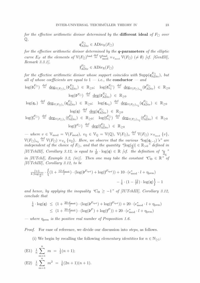
INTER-UNIVERSAL TEICHMULLER THEORY IV 23
for the effective arithmetic divisor determined by the different ideal of F� overQ,
qF�ADiv ∈ ADivR(F�)
for the effective arithmetic divisor determined by the q-parameters of the elliptic
curve EF at the elements of V(F�)baddef= Vbad
mod ×VmodV(F�) ( �= ∅) [cf. [GenEll],
Remark 3.3.1],
fF�ADiv ∈ ADivR(F�)
for the effective arithmetic divisor whose support coincides with Supp(qF�ADiv), but
all of whose coefficients are equal to 1 — i.e., the conductor — and
log(dF�v )
def= degV(F�)v
(dF�ADiv) ∈ R≥0; log(d
F�vQ )
def= degV(F�)vQ
(dF�ADiv) ∈ R≥0
log(dF�)def= deg(d
F�ADiv) ∈ R≥0
log(qv)def= degV(F�)v
(qF�ADiv) ∈ R≥0; log(qvQ
)def= degV(F�)vQ
(qF�ADiv) ∈ R≥0
log(q)def= deg(q
F�ADiv) ∈ R≥0
log(fF�v )
def= degV(F�)v
(fF�ADiv) ∈ R≥0; log(f
F�vQ
)def= degV(F�)vQ
(fF�ADiv) ∈ R≥0
log(fF�)def= deg(f
F�ADiv) ∈ R≥0
— where v ∈ Vmod = V(Fmod), vQ ∈ VQ = V(Q), V(F�)vdef= V(F�) ×Vmod
{v},V(F�)vQ
def= V(F�) ×VQ
{vQ}. Here, we observe that the various “log(q(−))’s” areindependent of the choice of F�, and that the quantity “|log(q)| ∈ R>0” defined in
[IUTchIII], Corollary 3.12, is equal to 12l · log(q) ∈ R [cf. the definition of “q
v”
in [IUTchI], Example 3.2, (iv)]. Then one may take the constant “CΘ ∈ R” of[IUTchIII], Corollary 3.12, to be
l+14·|log(q)| ·
{(1 + 12·dmod
l ) · (log(dFtpd) + log(fFtpd)) + 10 · (e∗mod · l + ηprm)
− 16 · (1− 12
l2 ) · log(q)}− 1
and hence, by applying the inequality “CΘ ≥ −1” of [IUTchIII], Corollary 3.12,conclude that
16 · log(q) ≤ (1 + 20·dmod
l ) · (log(dFtpd) + log(fFtpd)) + 20 · (e∗mod · l + ηprm)
≤ (1 + 20·dmod
l ) · (log(dF ) + log(fF )) + 20 · (e∗mod · l + ηprm)
— where ηprm is the positive real number of Proposition 1.6.
Proof. For ease of reference, we divide our discussion into steps, as follows.
(i) We begin by recalling the following elementary identities for n ∈ N≥1:
(E1) 1n
n∑m=1
m = 12 (n+ 1);
(E2) 1n
n∑m=1
m2 = 16 (2n+ 1)(n+ 1).
24 SHINICHI MOCHIZUKI
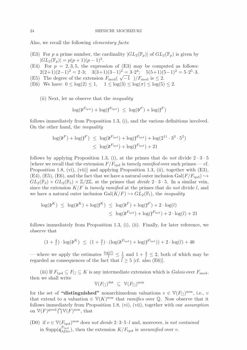
Also, we recall the following elementary facts:
(E3) For p a prime number, the cardinality |GL2(Fp)| of GL2(Fp) is given by|GL2(Fp)| = p(p+ 1)(p− 1)2.
(E4) For p = 2, 3, 5, the expression of (E3) may be computed as follows:2(2+1)(2−1)2 = 2·3; 3(3+1)(3−1)2 = 3·24; 5(5+1)(5−1)2 = 5·25 ·3.
(E5) The degree of the extension Fmod(√−1 )/Fmod is ≤ 2.
(E6) We have: 0 ≤ log(2) ≤ 1, 1 ≤ log(3) ≤ log(π) ≤ log(5) ≤ 2.
(ii) Next, let us observe that the inequality
log(dFtpd) + log(fFtpd) ≤ log(dF ) + log(fF )
follows immediately from Proposition 1.3, (i), and the various definitions involved.On the other hand, the inequality
log(dF ) + log(fF ) ≤ log(dFtpd) + log(fFtpd) + log(211 · 33 · 52)≤ log(dFtpd) + log(fFtpd) + 21
follows by applying Proposition 1.3, (i), at the primes that do not divide 2 · 3 · 5[where we recall that the extension F/Ftpd is tamely ramified over such primes — cf.Proposition 1.8, (vi), (vii)] and applying Proposition 1.3, (ii), together with (E3),(E4), (E5), (E6), and the fact that we have a natural outer inclusion Gal(F/Ftpd) ↪→GL2(F3) × GL2(F5) × Z/2Z, at the primes that divide 2 · 3 · 5. In a similar vein,since the extension K/F is tamely ramified at the primes that do not divide l, andwe have a natural outer inclusion Gal(K/F ) ↪→ GL2(Fl), the inequality
log(dK) ≤ log(dK) + log(fK) ≤ log(dF ) + log(fF ) + 2 · log(l)≤ log(dFtpd) + log(fFtpd) + 2 · log(l) + 21
follows immediately from Proposition 1.3, (i), (ii). Finally, for later reference, weobserve that
(1 + 4l ) · log(dK) ≤ (1 + 4
l ) · (log(dFtpd) + log(fFtpd)) + 2 · log(l) + 46
— where we apply the estimates log(l)l ≤ 1
2 and 1 + 4l ≤ 2, both of which may be
regarded as consequences of the fact that l ≥ 5 [cf. also (E6)].
(iii) If Ftpd ⊆ F� ⊆ K is any intermediate extension which is Galois over Fmod,then we shall write
V(F�)dst ⊆ V(F�)
non
for the set of “distinguished” nonarchimedean valuations v ∈ V(F�)non, i.e., vthat extend to a valuation ∈ V(K)non that ramifies over Q. Now observe that itfollows immediately from Proposition 1.8, (vi), (vii), together with our assumptionon V(F )good
⋂V(F )non, that
(D0) if v ∈ V(Ftpd)non does not divide 2 ·3 ·5 · l and, moreover, is not contained
in Supp(qFtpd
ADiv), then the extension K/Ftpd is unramified over v.
INTER-UNIVERSAL TEICHMULLER THEORY IV 25
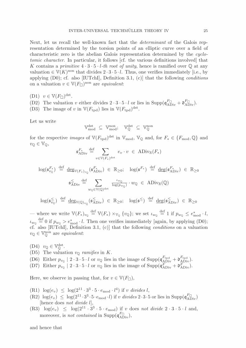
Next, let us recall the well-known fact that the determinant of the Galois rep-resentation determined by the torsion points of an elliptic curve over a field ofcharacteristic zero is the abelian Galois representation determined by the cyclo-tomic character. In particular, it follows [cf. the various definitions involved] thatK contains a primitive 4 · 3 · 5 · l-th root of unity, hence is ramified over Q at anyvaluation ∈ V(K)non that divides 2 · 3 · 5 · l. Thus, one verifies immediately [i.e., byapplying (D0); cf. also [IUTchI], Definition 3.1, (c)] that the following conditionson a valuation v ∈ V(F�)non are equivalent:
(D1) v ∈ V(F�)dst.(D2) The valuation v either divides 2 · 3 · 5 · l or lies in Supp(q
F�ADiv + d
F�ADiv).
(D3) The image of v in V(Ftpd) lies in V(Ftpd)dst.
Let us write
Vdstmod ⊆ Vnon
mod; VdstQ ⊆ Vnon
Q
for the respective images of V(Ftpd)dst in Vmod, VQ and, for F∗ ∈ {Fmod,Q} and
vQ ∈ VQ,
sF∗ADiv
def=
∑v∈V(F∗)dst
ev · v ∈ ADivR(F∗)
log(sF∗vQ)
def= degV(F∗)vQ
(sF∗ADiv) ∈ R≥0; log(sF∗)
def= deg(sF∗
ADiv) ∈ R≥0
s≤ADivdef=
∑wQ∈V(Q)dst
ιwQ
log(pwQ) · wQ ∈ ADivR(Q)
log(s≤vQ)
def= degV(Q)vQ
(s≤ADiv) ∈ R≥0; log(s≤) def= deg(s≤ADiv) ∈ R≥0
— where we write V(F∗)vQ
def= V(F∗) ×VQ
{vQ}; we set ιwQ
def= 1 if pwQ
≤ e∗mod · l,ιwQ
def= 0 if pwQ
> e∗mod · l. Then one verifies immediately [again, by applying (D0);cf. also [IUTchI], Definition 3.1, (c)] that the following conditions on a valuationvQ ∈ Vnon
Q are equivalent:
(D4) vQ ∈ VdstQ .
(D5) The valuation vQ ramifies in K.
(D6) Either pvQ | 2 · 3 · 5 · l or vQ lies in the image of Supp(qFtpd
ADiv + dFtpd
ADiv).
(D7) Either pvQ | 2 · 3 · 5 · l or vQ lies in the image of Supp(qFADiv + dFADiv).
Here, we observe in passing that, for v ∈ V(F�),
(R1) log(ev) ≤ log(211 · 33 · 5 · emod · l4) if v divides l,
(R2) log(ev) ≤ log(211 ·33 ·5 ·emod · l) if v divides 2 ·3 ·5 or lies in Supp(qF�ADiv)
[hence does not divide l],(R3) log(ev) ≤ log(211 · 33 · 5 · emod) if v does not divide 2 · 3 · 5 · l and,
moreover, is not contained in Supp(qF�ADiv),
and hence that
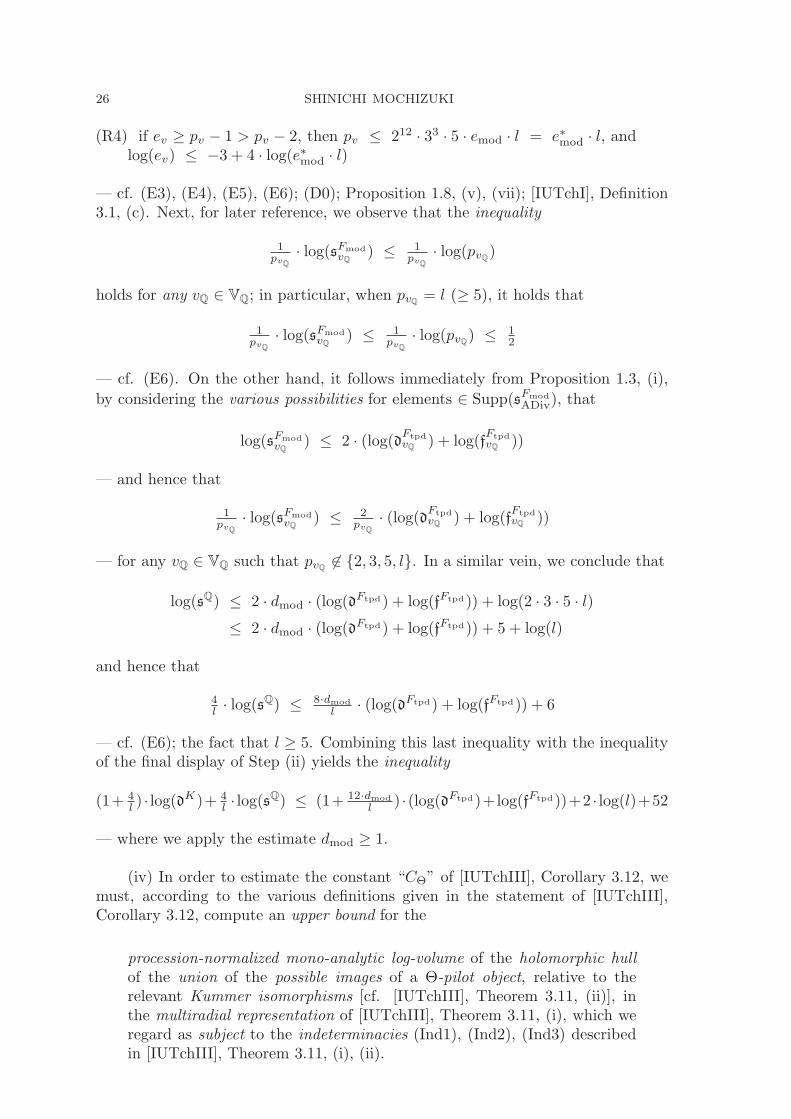
26 SHINICHI MOCHIZUKI
(R4) if ev ≥ pv − 1 > pv − 2, then pv ≤ 212 · 33 · 5 · emod · l = e∗mod · l, andlog(ev) ≤ −3 + 4 · log(e∗mod · l)
— cf. (E3), (E4), (E5), (E6); (D0); Proposition 1.8, (v), (vii); [IUTchI], Definition3.1, (c). Next, for later reference, we observe that the inequality
1pvQ
· log(sFmodvQ
) ≤ 1pvQ
· log(pvQ)
holds for any vQ ∈ VQ; in particular, when pvQ= l (≥ 5), it holds that
1pvQ
· log(sFmodvQ
) ≤ 1pvQ
· log(pvQ) ≤ 1
2
— cf. (E6). On the other hand, it follows immediately from Proposition 1.3, (i),
by considering the various possibilities for elements ∈ Supp(sFmod
ADiv), that
log(sFmodvQ
) ≤ 2 · (log(dFtpdvQ ) + log(f
FtpdvQ ))
— and hence that
1pvQ
· log(sFmodvQ
) ≤ 2pvQ
· (log(dFtpdvQ ) + log(f
FtpdvQ ))
— for any vQ ∈ VQ such that pvQ �∈ {2, 3, 5, l}. In a similar vein, we conclude that
log(sQ) ≤ 2 · dmod · (log(dFtpd) + log(fFtpd)) + log(2 · 3 · 5 · l)≤ 2 · dmod · (log(dFtpd) + log(fFtpd)) + 5 + log(l)
and hence that
4l · log(sQ) ≤ 8·dmod
l · (log(dFtpd) + log(fFtpd)) + 6
— cf. (E6); the fact that l ≥ 5. Combining this last inequality with the inequalityof the final display of Step (ii) yields the inequality
(1+ 4l ) · log(dK)+ 4
l · log(sQ) ≤ (1+ 12·dmod
l ) ·(log(dFtpd)+log(fFtpd))+2 · log(l)+52
— where we apply the estimate dmod ≥ 1.
(iv) In order to estimate the constant “CΘ” of [IUTchIII], Corollary 3.12, wemust, according to the various definitions given in the statement of [IUTchIII],Corollary 3.12, compute an upper bound for the
procession-normalized mono-analytic log-volume of the holomorphic hullof the union of the possible images of a Θ-pilot object, relative to therelevant Kummer isomorphisms [cf. [IUTchIII], Theorem 3.11, (ii)], inthe multiradial representation of [IUTchIII], Theorem 3.11, (i), which weregard as subject to the indeterminacies (Ind1), (Ind2), (Ind3) describedin [IUTchIII], Theorem 3.11, (i), (ii).
INTER-UNIVERSAL TEICHMULLER THEORY IV 27
Thus, we proceed to estimate this log-volume at each vQ ∈ VQ. Once one fixes vQ,this amounts to estimating the component of this log-volume in
“IQ(S±j+1
;n,◦D�vQ)”
[cf. the notation of [IUTchIII], Theorem 3.11, (i), (a)], for each j ∈ {1, . . . , l�},which we shall also regard as an element of F�
l , and then computing the average,over j ∈ {1, . . . , l�}, of these estimates. Here, we recall [cf. [IUTchI], Proposition6.9, (i); [IUTchIII], Proposition 3.4, (ii)] that S±j+1 = {0, 1, . . . , j}. Also, we recall
from [IUTchIII], Proposition 3.2, that “IQ(S±j+1
;n,◦D�vQ)” is, by definition, a tensor
product of j+1 copies, indexed by the elements of S±j+1, of the direct sum of the Q-
spans of the log-shells associated to each of the elements of V(Fmod)vQ[cf., especially,
the second and third displays of [IUTchIII], Proposition 3.2]. In particular, for eachcollection
{vi}i∈S±j+1
of [not necessarily distinct!] elements of V(Fmod)vQ, we must estimate the com-
ponent of the log-volume in question corresponding to the tensor product of theQ-spans of the log-shells associated to this collection {vi}i∈S±
j+1and then compute
the weighted average [cf. the discussion of Remark 1.7.1], over possible collections{vi}i∈S±
j+1, of these estimates.
(v) Let vQ ∈ VdstQ . Fix j, {vi}i∈S±
j+1as in Step (iv). Write vi ∈ V
∼→ Vmod =
V(Fmod) for the element corresponding to vi. We would like to apply Proposition1.4, (iii), to the present situation, by taking
· “I” to be S±j+1;· “I∗ ⊆ I” to be the set of i ∈ I such that evi
> pvQ− 2;
· “ki” to be Kvi[so “Ri” will be the ring of integers OKvi
of Kvi];
· “i†” to be j ∈ S±j+1;
· “λ” to be 0 if vj ∈ Vgood;
· “λ” to be “ord(−)” of the element qj2
vj
[cf. the definition of “qv” in
[IUTchI], Example 3.2, (iv)] if vj ∈ Vbad.
Thus, the inclusion “φ(pλ · (RI)∼) ⊆ p�λ−dI−aI� · logp(R×
I )” of Proposition 1.4,(iii), implies that the result of multiplying the tensor product of log-shells underconsideration by a suitable nonpositive [cf. the inequalities concerning “dI+aI” thatconstitute the final portion of Proposition 1.4, (iii)] integer power of pvQ
containsthe “union of possible images of a Θ-pilot object” discussed in Step (iv). That is tosay, the indeterminacies (Ind1) and (Ind2) are taken into account by the arbitrarynature of the automorphism “φ” [cf. Proposition 1.2], while the indeterminacy(Ind3) is taken into account by the fact that we are considering upper bounds [cf.the discussion of Step (x) of the proof of [IUTchIII], Corollary 3.12], together withthe fact that the above-mentioned integer power of pvQ is nonpositive, which impliesthat the module obtained by multiplying by this power of pvQ contains the tensorproduct of log-shells under consideration. Thus, an upper bound on the component
28 SHINICHI MOCHIZUKI
of the log-volume of the holomorphic hull under consideration may be obtained bycomputing an upper bound for the log-volume of the right-hand side of the inclusion“p�λ−dI−aI� · logp(R×
I ) ⊆ p�λ−dI−aI�−bI · (RI)∼” of Proposition 1.4, (iii). Such an
upper bound
“(− λ+ dI + 1
)· log(p) +
∑i∈I∗
{3 + log(ei)}”
is given in the second displayed inequality of Proposition 1.4, (iii). Here, we notethat if evi
≤ pvQ− 2 for all i ∈ I, then this upper bound assumes the form
“(− λ+ dI + 1
)· log(p)”.
On the other hand, by (R4), if evi> pvQ − 2 for some i ∈ I, then it follows that
pvQ≤ e∗mod · l, and log(evi
) ≤ −3+4 · log(e∗mod · l), so the upper bound in questionmay be taken to be
“(− λ+ dI + 1
)· log(p) + 4(j + 1) · l∗mod”
— where we write l∗moddef= log(e∗mod · l). Also, we note that, unlike the other terms
that appear in these upper bounds, “λ” is asymmetric with respect to the choiceof “i† ∈ I” in S±j+1. Since we would like to compute weighted averages [cf. the
discussion of Remark 1.7.1], we thus observe that, after symmetrizing with respectto the choice of “i† ∈ I” in S±j+1, this upper bound may be written in the form
“β�e”
[cf. the notation of Proposition 1.7] if, in the situation of Proposition 1.7, one takes
· “E” to be V(Fmod)vQ ;· “n” to be j + 1, so an element “�e ∈ En” corresponds precisely to acollection {vi}i∈S±
j+1;
· “λe”, for an element e ∈ E corresponding to v ∈ V(Fmod) = Vmod, to be[(Fmod)v : QvQ
] ∈ R>0;· “βe”, for an element e ∈ E corresponding to v ∈ V(Fmod) = Vmod, to be
log(dKv )− j2
2l(j+1) · log(qv) + 1j+1 · log(pvQ) + 4 · ιvQ · l∗mod
— where we recall that ιvQdef= 1 if pvQ ≤ e∗mod · l, ιvQ
def= 0 if pvQ
> e∗mod · l.
Here, we note that it follows immediately from the first equality of the first dis-play of Proposition 1.7 that, after passing to weighted averages, the operation ofsymmetrizing with respect to the choice of “i† ∈ I” in S±j+1 does not affect the com-putation of the upper bound under consideration. Thus, by applying Proposition1.7, we obtain that the resulting “weighted average upper bound” is given by
(j + 1) · log(dKvQ)− j2
2l · log(qvQ) + log(sQvQ) + 4(j + 1) · l∗mod · log(s≤vQ)
INTER-UNIVERSAL TEICHMULLER THEORY IV 29
— where we recall the notational conventions introduced in Step (iii). Thus, itremains to compute the average over j ∈ F�
l . By averaging over j ∈ {1, . . . , l� =l−12 } and applying (E1), (E2), we obtain the “procession-normalized upper
bound”
(l�+3)2 · log(dKvQ
)− (2l�+1)(l�+1)12l · log(qvQ) + log(sQvQ
) + 2(l� + 3) · l∗mod · log(s≤vQ)
= l+54 · log(dKvQ)− l+1
24 · log(qvQ) + log(sQvQ) + (l + 5) · l∗mod · log(s≤vQ)
≤ l+14 ·
{(1 + 4
l ) · log(dKvQ)− 16 · log(qvQ) + 4
l · log(sQvQ) + 203 · l∗mod · log(s≤vQ
)
}
— where, in the passage to the final displayed inequality, we apply the estimates1
l+1 ≤ 1l and 4(l+5)
l+1 ≤ 203 , both of which may be regarded as consequences of the
fact that l ≥ 5.
(vi) Next, let vQ ∈ VnonQ \ Vdst
Q . Fix j, {vi}i∈S±j+1
as in Step (iv). Write
vi ∈ V∼→ Vmod = V(Fmod) for the element corresponding to vi. We would like to
apply Proposition 1.4, (iv), to the present situation, by taking
· “I” to be S±j+1;
· “ki” to be Kvi[so “Ri” will be the ring of integers OKvi
of Kvi].
Here, we note that our assumption that vQ ∈ VnonQ \Vdst
Q implies that the hypothesesof Proposition 1.4, (iv), are satisfied. Thus, the inclusion “φ((RI)
∼) ⊆ (RI)∼” of
Proposition 1.4, (iv), implies that the tensor product of log-shells under consider-ation contains the “union of possible images of a Θ-pilot object” discussed in Step(iv). That is to say, the indeterminacies (Ind1) and (Ind2) are taken into accountby the arbitrary nature of the automorphism “φ” [cf. Proposition 1.2], while theindeterminacy (Ind3) is taken into account by the fact that we are considering upperbounds [cf. the discussion of Step (x) of the proof of [IUTchIII], Corollary 3.12],together with the fact that the “container of possible images” is precisely equal tothe tensor product of log-shells under consideration. Thus, an upper bound on thecomponent of the log-volume under consideration may be obtained by computingan upper bound for the log-volume of the right-hand side “(RI)
∼” of the aboveinclusion. Such an upper bound
“0”
is given in the final equality of Proposition 1.4, (iv). One may then compute a“weighted average upper bound” and then a “procession-normalized upperbound”, as was done in Step (v). The resulting “procession-normalized upperbound” is clearly equal to 0.
(vii) Next, let vQ ∈ VarcQ . Fix j, {vi}i∈S±
j+1as in Step (iv). Write vi ∈
V∼→ Vmod = V(Fmod) for the element corresponding to vi. We would like to
apply Proposition 1.5, (iii), (iv), to the present situation, by taking
· “I” to be S±j+1 [so |I| = j + 1];
· “V ” to be V(Fmod)vQ;
30 SHINICHI MOCHIZUKI
· “Cv” to be Kv, where we write v ∈ V∼→ Vmod for the element determined
by v ∈ V .
Then it follows from Proposition 1.5, (iii), (iv), that
πj+1 ·BI
serves as a container for the “union of possible images of a Θ-pilot object” discussedin Step (iv). That is to say, the indeterminacies (Ind1) and (Ind2) are taken intoaccount by the fact that BI ⊆ MI is preserved by arbitrary automorphisms of thetype discussed in Proposition 1.5, (iii), while the indeterminacy (Ind3) is taken intoaccount by the fact that we are considering upper bounds [cf. the discussion ofStep (x) of the proof of [IUTchIII], Corollary 3.12], together with the fact that, byProposition 1.5, (iv), together with our choice of the factor πj+1, this “container ofpossible images” contains the elements of MI obtained by forming the tensor prod-uct of elements of the log-shells under consideration. Thus, an upper bound on thecomponent of the log-volume under consideration may be obtained by computingan upper bound for the log-volume of this container. Such an upper bound
(j + 1) · log(π)follows immediately from the fact that [in order to ensure compatibility with arith-metic degrees of arithmetic line bundles — cf. [IUTchIII], Proposition 3.9, (iii) —one is obliged to adopt normalizations which imply that] the log-volume of BI isequal to 0. One may then compute a “weighted average upper bound” andthen a “procession-normalized upper bound”, as was done in Step (v). The resulting“procession-normalized upper bound” is given by
l+54 · log(π) ≤ l+1
4 · 4— cf. (E1), (E6); the fact that l ≥ 5.
(viii) Now we return to the discussion of Step (iv). In order to compute thedesired upper bound for “CΘ”, it suffices to sum over vQ ∈ VQ the various local“procession-normalized upper bounds” obtained in Steps (v), (vi), (vii) forvQ ∈ VQ. By applying the inequality of the final display of Step (iii), we thus obtainthe following upper bound for “CΘ ·|log(q)|”, i.e., the product of “CΘ” and 1
2l ·log(q):
l+14 ·
{(1 + 12·dmod
l ) · (log(dFtpd) + log(fFtpd)) + 2 · log(l) + 56− 16 · (1− 12
l2 ) · log(q)
+ 203 · l∗mod · log(s≤)
}− 1
2l · log(q)
— where we apply the estimate l+14 · 1
6 · 12l2 ≥ 1
2l [cf. the fact that l ≥ 1].
Now let us recall the constant “ηprm” of Proposition 1.6. By applying Propo-sition 1.6, we compute:
l∗mod · log(s≤) ≤ log(e∗mod · l) ·∑
p ≤ e∗mod
·l1 ≤ 4
3 · log(e∗mod · l) · e∗mod·llog(e∗
mod·l)
= 43 · e∗mod · l
INTER-UNIVERSAL TEICHMULLER THEORY IV 31
— where the sum ranges over the primes p ≤ e∗mod · l — if e∗mod · l ≥ ηprm;
l∗mod · log(s≤) ≤ log(e∗mod · l) ·∑
p ≤ e∗mod
·l1 ≤ 4
3 · log(ηprm) · ηprm
log(ηprm)
= 43 · ηprm
— where the sum ranges over the primes p ≤ e∗mod · l — if e∗mod · l < ηprm. Thus,we conclude that
l∗mod · log(s≤) ≤ 43 · (e∗mod · l + ηprm)
[i.e., regardless of the size of e∗mod · l]. Also, let us observe that
13 · 4
3 · (e∗mod · l + ηprm) ≥ 13 · 4
3 · e∗mod · l ≥ 2 · 2 · 212 · 3 · 5 · l ≥ 2 · log(l) + 56
— where we apply the estimates emod ≥ 1, 212 · 3 · 5 ≥ 56, l ≥ 5 ≥ 1, l ≥ log(l)[cf. the fact that l ≥ 5]. Thus, substituting back into our original upper bound for“CΘ · |log(q)|”, we obtain the following upper bound for “CΘ”:
l+14·|log(q)| ·
{(1 + 12·dmod
l ) · (log(dFtpd) + log(fFtpd)) + 10 · (e∗mod · l + ηprm)
− 16 · (1− 12
l2 ) · log(q)}− 1
— where we apply the estimate 20+13 · 4
3 = 7·43 ≤ 10 — i.e., as asserted in the
statement of Theorem 1.10. The final portion of Theorem 1.10 follows immediatelyfrom [IUTchIII], Corollary 3.12, by applying the inequality of the first display ofStep (ii), together with the estimates
(1− 12l2 )
−1 ≤ 2; (1− 12l2 )
−1 · (1 + 12·dmod
l ) ≤ 1 + 20·dmod
l
[cf. the fact that l ≥ 7, dmod ≥ 1]. ©
Remark 1.10.1. One of the main original motivations for the development ofthe theory discussed in the present series of papers was to create a framework, orgeometry, within which a suitable analogue of the scheme-theoretic Hodge-Arakelovtheory of [HASurI], [HASurII] could be realized in such a way that the obstruc-tions to diophantine applications that arose in the scheme-theoretic formulation of[HASurI], [HASurII] [cf. the discussion of [HASurI], §1.5.1; [HASurII], Remark 3.7]could be avoided. From this point of view, it is of interest to observe that the com-putation of the “leading term” of the inequality of the final display of the statementof Theorem 1.10 — i.e., of the term
(l�+3)2 · log(dKvQ)− (2l�+1)(l�+1)
12l · log(qvQ)
that occurs in the final display of Step (v) of the proof of Theorem 1.10 — via theidentities (E1), (E2) is essentially identical to the computation of the leading termthat occurs in the proof of [HASurI], Theorem A [cf. the discussion following thestatement of Theorem A in [HASurI], §1.1]. That is to say, in some sense,
32 SHINICHI MOCHIZUKI
the computations performed in the proof of Theorem 1.10 were alreadyessentially known to the author around the year 2000; the problem thenwas to construct an appropriate framework, or geometry, in whichthese computations could be performed!
This sort of situation may be compared to the computations underlying the WeilConjectures priori to the construction of a “Weil cohomology” in which thosecomputations could be performed, or, alternatively, to various computations ofinvariants in topology or differential geometry that were motivated by computationsin physics, again prior to the construction of a suitable mathematical frameworkin which those computations could be performed.
Remark 1.10.2. The computation performed in the proof of Theorem 1.10 maybe thought of as the computation of a sort of derivative in the F�
l -direction,which, relative to the analogy between the theory of the present series of papersand the p-adic Teichmuller theory of [pOrd], [pTeich], corresponds to the derivativeof the canonical Frobenius lifting — cf. the discussion of [IUTchIII], Remark 3.12.4,(iii). In this context, it is useful to recall the arithmetic Kodaira-Spencer morphismthat occurs in scheme-theoretic Hodge-Arakelov theory [cf. [HASurII], §3]. Inparticular, in [HASurII], Corollary 3.6, it is shown that, when suitably formulated,a “certain portion” of this arithmetic Kodaira-Spencer morphism coincides with theusual geometric Kodaira-Spencer morphism. From the point of view of the actionof GL2(Fl) on the l-torsion points involved, this “certain portion” consists of theunipotent matrices (
1 ∗0 1
)of GL2(Fl). By contrast, the F�
l -symmetries that occur in the present series ofpapers correspond to the toral matrices( ∗ 0
0 ∗
)
of GL2(Fl) — cf. the discussion of [IUTchI], Example 4.3, (i). As we shall see in§2 below, in the present series of papers, we shall ultimately take l to be “large”.When l is “sufficiently large”, GL2(Fl) may be thought of as a “good approximation”for GL2(Z) or GL2(R) — cf. the discussion of [IUTchI], Remark 6.12.3, (i), (iii).In the case of GL2(R), “toral subgroups” may be thought of as corresponding tothe isotropy subgroups [isomorphic to S1] of points that arise from the action ofGL2(R) on the upper half-plane, i.e., subgroups which may be thought of as a sortof geometric, group-theoretic representation of tangent vectors at a point.
Remark 1.10.3. The “terms involving l” that occur in the inequality of thefinal display of Theorem 1.10 may be thought of as an inevitable consequence of thefundamental role played in the theory of the present series of papers by the l-torsionpoints of the elliptic curve under consideration. Here, we note that it is of crucialimportance to work over the field of rationality of the l-torsion points [i.e., “K” asopposed to “F”] not only when considering the global portions of the various ΘNF-
INTER-UNIVERSAL TEICHMULLER THEORY IV 33
and Θ±ell-Hodge theaters involved, but also when considering the local portions —i.e., the prime-strips — of these ΘNF- and Θ±ell-Hodge theaters. That is to say,these local portions are necessary, for instance, in order to glue together the ΘNF-and Θ±ell-Hodge theaters that appear so as to form a Θ±ellNF-Hodge theater [cf.the discussion of [IUTchI], Remark 6.12.2]. In particular, to allow, within theselocal portions, any sort of “Galois indeterminacy” with respect to the l-torsionpoints — even, for instance, at v ∈ V
good⋂V
non, which, at first glance, mightappear irrelevant to the theory of Hodge-Arakelov-theoretic evaluation at l-torsionpoints developed in [IUTchII] — would have the effect of invalidating the variousdelicate manipulations involving l-torsion points discussed in [IUTchI], §4, §6 [cf.,e.g., [IUTchI], Propositions 4.7, 6.5].
Remark 1.10.4. The various fluctuations in log-volume — i.e., whose computa-tion is the subject of Theorem 1.10! — that arise from themultiradial representationof [IUTchIII], Theorem 3.11, (i), may be thought of as a sort of “inter-universalanalytic torsion”. Indeed,
in general, “analytic torsion”may be understood as a sort ofmeasure—in “metrized” [e.g., log-volume!] terms — of the degree of deviation ofthe “holomorphic functions” [such as sections of a line bundle] on a variety— i.e., which depend, in an essential way, on the holomorphic moduliof the variety! — from the “real analytic functions” — i.e., which areinvariant with respect to deformations of the holomorphic moduliof the variety.
For instance:
(a) In “classical” Arakelov theory, analytic torsion typically arises as [the log-arithm of] a sort of normalized determinant of the Laplacian acting on somespace of real analytic [or L2-] sections of a line bundle on a complex variety equippedwith a real analytic Kahler metric [cf., e.g., [Arak], Chapters V, VI]. Here, we recallthat in this sort of situation, the space of holomorphic sections of the line bundleis given by the kernel of the Laplacian; the definition of the Laplacian depends, inan essential way, on the Kahler metric, hence, in particular, on the holomorphicmoduli of the variety under consideration [cf., e.g., the case of the Poincare metricon a hyperbolic Riemann surface!].
(b) In the scheme-theoretic Hodge-Arakelov theory discussed in [HASurI], [HA-SurII], the main theorem consists of a sort of comparison isomorphism [cf. [HASurI],Theorem A] between a certain subspace of the space of global sections of the pull-back of an ample line bundle on an elliptic curve to the universal vectorial extensionof the elliptic curve and the space of set-theoretic functions on the torsion points ofthe elliptic curve. That is to say, the former space of sections contains, in a natu-ral way, the space of holomorphic sections of the ample line bundle on the ellipticcurve, while the latter space of functions may be thought of as a sort of “discreteapproximation” of the space of real analytic functions on the elliptic curve [cf. thediscussion of [HASurI], §1.3.2, §1.3.4]. In this context, the “Gaussian poles” [cf.the discussion of [HASurI], §1.1] arise as a measure of the discrepancy of integralstructures between these two spaces in a neighborhood of the divisor at infinity of
34 SHINICHI MOCHIZUKI
the moduli stack of elliptic curves, hence may be thought of as a sort of “analytictorsion at the divisor at infinity” [cf. the discussion of [HASurI], §1.2].
(c) In the case of the multiradial representation of [IUTchIII], Theorem 3.11,(i), the fluctuations of log-volume computed in Theorem 1.10 arise precisely as aresult of the execution of a comparison of an “alien” arithmetic holomorphicstructure to this multiradial representation, which is compatible with the per-mutation symmetries of the etale-picture, i.e., which is “invariant with respect todeformations of the arithmetic holomorphic moduli of the number field under con-sideration” in the sense that it makes sense simultaneously with respect to distinctarithmetic holomorphic structures [cf. [IUTchIII], Remark 3.11.1; [IUTchIII], Re-mark 3.12.3, (ii)]. Here, it is of interest to observe that the object of this comparisonconsists of the values of the theta function, i.e., in essence, a “holomorphic sectionof an ample line bundle”. In particular, the resulting fluctuations of log-volumemay be thought as a sort of “analytic torsion”. By analogy to the terminology“Gaussian poles” discussed in (b) above, it is natural to think of the terms involv-ing the different dK(−) that appear in the computation underlying Theorem 1.10 [cf.,
e.g., the final display of Step (v) of the proof of Theorem 1.10] as “differentialpoles” [cf. the discussion of Remarks 1.10.1, 1.10.2]. Finally, in the context of thenormalized determinants that appear in (a), it is interesting to note the role playedby the prime number theorem — i.e., in essence, the Riemann zeta func-tion [cf. Proposition 1.6 and its proof] — in the computation of “inter-universalanalytic torsion” given in the proof of Theorem 1.10.
Remark 1.10.5. The above remarks focused on the conceptual aspects of thetheory surrounding Theorem 1.10. Before proceeding, however, we pause to discussbriefly certain aspects of Theorem 1.10 that are of interest from a computationalpoint of view, i.e., in the spirit of conventional analytic number theory.
(i) First, we begin by observing that, unlike the inequalities that appear in thevarious results [cf. Corollaries 2.2, (ii); 2.3] obtained in §2 below, the inequalitiesobtained in Theorem 1.10 involve only essentially explicit constants and, more-over, do not require one to exclude some non-explicit finite set of “isomorphismclasses of exceptional elliptic curves”. From this point of view,
the inequalities obtained in Theorem 1.10 are suited to application tocomputations concerning various explicit diophantine equations,such as, for instance, the equations that appear in “Fermat’s Last Theo-rem”.
Such explicit computations in the case of specific diophantine equations are, how-ever, beyond the scope of the present paper.
(ii) One topic of interest in the context of computational aspects of Theorem1.10 is the asymptotic behavior of the bound that appears in, say, the firstinequality of the final display of Theorem 1.10. Let us assume, for simplicity,
that Ftpd = Q [so dmod = 1]. Also, to simplify the notation, let us write δdef=
log(dFtpd) + log(fFtpd) = log(fFtpd). Then the bound under consideration assumesthe form
δ + ∗ · δl + ∗ · l + ∗
INTER-UNIVERSAL TEICHMULLER THEORY IV 35
— where, in the present discussion, the “∗’s” are to be understood as denoting fixedpositive real numbers. Thus, the leading term [cf. the discussion of Remark 1.10.1]is equal to δ. The remaining terms give rise to the “ε terms” [and bounded discrep-ancy] of the inequalities of Corollaries 2.2, (ii); 2.3, obtained in §2 below. Thus,if one ignores “bounded discrepancies”, it is of interest to consider the behavior ofthe “ε terms”
∗ · δl + ∗ · l
as one allows the initial Θ-data under consideration to vary [i.e., subject to thecondition “Ftpd = Q”]. In this context, one fundamental observation is the fol-lowing: although l is subject to various other conditions, no matter how “skillfully”one chooses l, the resulting “ε terms” are always
≥ ∗ · δ1/2
— an estimate that may be obtained by thinking of l as ≈ δα, for some realnumber α, and comparing δα and δ1−α. This estimate is of particular interestin the context of various explicit examples constructed by Masser and others [cf.[Mss]; the discussion of [vFr], §2] in which explicit “abc sums” are constructed forwhich the quantity on the left-hand side of the inequality of Theorem 1.10 underconsideration exceeds the order of δ +
∗ · δ1/2
log(δ)
— cf. [vFr], Equation (6). In particular, the asymptotic estimates given by Theorem1.10 are consistent with the known asymptotic behavior of these explicit abc sums.Indeed, the exponent “ 1
2” that appears in the fundamental observation discussedabove coincides precisely with the “expectation” expressed by van Frankenhuijsenin the final portion of the discussion of [vFr], §2! In the present paper, although weare unable to in fact achieve bounds on the “ε terms” of the order ∗ · δ1/2, we dosucceed in obtaining bounds on the “ε terms” of the order
∗ · δ1/2 · log(δ)
— albeit under the assumption that the abc sums under consideration are com-pactly bounded away from infinity at the prime 2, as well as at the archimedeanprime [cf. Corollary 2.2, (ii); Remark 2.2.1 below for more details].
(iii) In the context of the discussion of (ii), it is of interest to observe thatthe “∗ · l” portion of the “ε terms” that appear arises from the estimates givenin Step (viii) of the proof of Theorem 1.10 for the quantity “log(s≤)”. From thepoint of view of the discussion of [vFr], §3, this quantity corresponds essentiallyto a “certain portion” of the quantity “ω(abc)” associated to an abc sum. Thatis to say, whereas “ω(abc)” denotes the total number of prime factors that occurin the product abc, the quantity “log(s≤)” corresponds, roughly speaking, to thenumber of these prime factors that are ≤ e∗mod · l. The appearance [i.e., in the proofof Theorem 1.10] of such a term which is closely related to “ω(abc)” is of interestfrom the point of view of the discussion of [vFr], §3, partly since it is [not preciselyidentical to, but nonetheless] reminiscent of the various refinements of the ABCConjecture proposed by Baker [i.e., which are the main topic of the discussion of
36 SHINICHI MOCHIZUKI
[vFr], §3]. The appearance [i.e., in the proof of Theorem 1.10] of such a term whichis closely related to “ω(abc)” is also of interest from the point of view of the explicit
abc sums discussed in (ii) that give rise to asymptotic behavior ≥ ∗ · δ1/2
log(δ) . That
is to say, according to the discussion of [vFr], §3, Remark 1, this sort of abc sumtends to give rise to a
relatively large value for ω(abc) — i.e., a state of affairs that is con-sistent with the crucial role played by the “ε term” related to ω(abc) inthe computation of the lower bound “≥ ∗ · δ1/2” that appears in thefundamental observation of (ii).
By contrast, the abc sums of the form “2n = p + qr” [where p, q, and r are primenumbers] considered in [vFr], §3, Remark 1, give rise to a
relatively small value for ω(abc) [indeed, ω(abc) ≤ 4] — i.e., a situationthat suggests relatively small/essentially negligible “ε terms” in the boundof Theorem 1.10 under consideration.
Such essentially negligible “ε terms” are, however, consistent with the fact [cf.[vFr], §3, Remark 1] that, for such abc sums, the left-hand side of the inequality ofTheorem 1.10 under consideration is roughly ≈ 1
2 · the leading term of the boundon the right-hand side, hence, in particular, is amply bounded by the leading termon the right-hand side, without any “help” from the “ε terms”.
Remark 1.10.6.
(i) In the context of the discussion of Remark 1.10.5, it is important to remem-ber that
the bound on “ 16 · log(q)” given in Theorem 1.10 only concerns the q-
parameters at the nonarchimedean valuations contained in Vbadmod, all of
which are necessarily of odd residue characteristic
— cf. [IUTchI], Definition 3.1, (b). This observation is of relevance to the examplesof abc sums constructed in [Mss] [cf. the discussion of Remark 1.10.5, (ii)], sinceit does not appear, at first glance, that there is any way to effectively control thecontributions at the prime 2 in these examples, that is to say, in the notation ofthe Proposition of [Mss], to control the power of 2 that divides the integer “c”of the Proposition of [Mss], or, alternatively, in the notation of the proof of thisProposition on [Mss], p. 22, to control the power of 2 that divides the difference“xi − xi−1”. On the other hand, it was pointed out to the author by A. Venkateshthat in fact it is not difficult to modify the construction of these examples of abcsums given in [Mss] so as to obtain similar asymptotic estimates to those obtainedin [Mss] [cf. the discussion of Remark 1.10.5, (ii)], even without taking into accountthe contributions at the prime 2.
(ii) In the context of the discussion of (i), it is of interest to recall why nonar-chimedean primes of even residue characteristic where the elliptic curve under
INTER-UNIVERSAL TEICHMULLER THEORY IV 37
consideration has bad multiplicative reduction are excluded from Vbadmod in the the-
ory of the present series of papers. In a word, the reason that the theory encountersdifficulties at primes over 2 is that it depends, in a quite essential way, on the theoryof the etale theta function developed in [EtTh], which fails at primes over 2 [cf.the assumption that “p is odd” in [EtTh], Theorem 1.10, (iii); [EtTh], Definition2.5; [EtTh], Corollary 2.18]. From the point of view of the theory of [IUTchI],[IUTchII], and [IUTchIII] [cf., especially, the theory of [IUTchII], §1, §2: [IUTchII],Corollary 1.12; [IUTchII], Corollary 2.4, (ii), (iii); [IUTchII], Corollary 2.6], one ofthe key consequences of the theory of [EtTh] is the simultaneous multiradialityof the algorithms that give rise to
(1) constant multiple rigidity and(2) cyclotomic rigidity.
At a more concrete level, (1) is obtained by evaluating the usual series for thetheta function [cf. [EtTh], Proposition 1.4] at the 2-torsion point in the “irreduciblecomponent labeled zero”. One computes easily that the resulting “special value” isa unit for odd p, but is equal to a [nonzero] non-unit when p = 2. In particular,since (1) is established by dividing the series of [EtTh], Proposition 1.4 [i.e., theusual series for the theta function], by this special value, it follows that
(a) the “integral structure” on the theta function determined by this specialvalue
coincides with
(b) the “integral structure” on the theta function determined by the naturalintegral structure on the pole at the origin
for odd p [cf. [EtTh], Theorem 1.10, (iii)], but not when p = 2. That is to say,when p = 2, a nontrivial denominator arises. Here, we recall that it is crucialto evaluate at 2-torsion points, i.e., as opposed to, say, more general points in theirreducible component labeled zero for reasons discussed in [IUTchII], Remark 2.5.1,(ii) [cf. also the discussion of [IUTchII], Remark 1.12.2, (i), (ii), (iii), (iv)]. Thisnontrivial denominator is fundamentally incompatible with the multiradiality of thealgorithms of (1), (2) in that it is incompatible with the fundamental splitting, or“decoupling”, into “purely radial” [i.e., roughly speaking, “value group”] and “purelycoric” [i.e., roughly speaking, “unit”] components discussed in [IUTchII], Remarks1.11.4, (i); 1.12.2, (vi) [cf. also the discussion of [IUTchII], Remark 1.11.5]. Thatis to say, on the one hand,
the multiradiality of (1) may only be established if the possible valuesat the evaluation points in the irreducible component labeled zero areknown, a priori, to be units, i.e., if one works relative to the integralstructure (a)
— cf. the discussion of [IUTchII], Remark 1.12.2, (i), (ii), (iii), (iv). On the otherhand, if one tries to work
38 SHINICHI MOCHIZUKI
simultaneously with the integral structure (b), hence with the non-trivial denominator discussed above, then the multiradiality of (2)is violated.
Here, we recall that the integral structure (b), which is referred to as the “canonicalintegral structure” in [EtTh], Proposition 1.4, (iii); [EtTh], Theorem 1.10, (iii), isin some sense the “integral structure of common sense”.
(iii) It is not entirely clear to the author at the time of writing to what extentthe integral structure (b) is necessary in order to carry out the theory developedin the present series of papers. Indeed, [EtTh], as well as the present series ofpapers, was written in a way that [unlike the discussion of (ii)!] “takes for granted”the fact that the two integral structures (a), (b) discussed above coincide for oddp, i.e., in a way which identifies these two integral structures and hence does notspecify, at various key points in the discussion, whether one is in fact working withintegral structure (a) or with integral structure (b). On the other hand, if it isindeed the case that not only the integral structure (a), but also the integral struc-ture (b) plays an essential role in the present series of papers, then it follows [cf.the discussion of (ii)!] that the theory of the present series of papers is funda-mentally incompatible with the inclusion in Vbad
mod of nonarchimedean primes ofeven residue characteristic where the elliptic curve under consideration has badmultiplicative reduction.
(iv) In the context of the discussion of (ii), (iii), it is perhaps useful to recallthat the classical theory of theta functions also tends to [depending on your pointof view!] “break down” or “assume a completely different form” at the prime 2. Forinstance, this phenomenon can be seen throughout Mumford’s theory of algebraictheta functions, which may be thought of as a sort of predecessor to the scheme-theoretic Hodge-Arakelov theory of [HASurI], [HASurII], which, in turn, may bethought of as a sort of predecessor to the theory of the present series of papers.In a similar vein, it is of interest to recall that the prime 2 is also excluded inthe p-adic Teichmuller theory of [pOrd], [pTeich]. This is done in order to avoidthe complications that occur in the theory of the Lie algebra sl2 over fields ofcharacteristic 2.
Remark 1.10.7.
(i) Since e∗mod ≤ d∗mod, one may replace “e∗mod” by “d∗mod” in the final twodisplays of the statement of Theorem 1.10.
(ii) By contrast, at least if one adheres to the framework of the theory of thepresent series of papers,
it is not possible to replace “dmod” by “emod” in the final two displaysof the statement of Theorem 1.10.
The fundamental reason for this is that, in the construction of the multiradialrepresentation of [IUTchIII], Theorem 3.11, (i), it is necessary to consider tensorproducts of copies, labeled by j ∈ F�
l , of Fmod over Q [cf. [IUTchIII], Proposition
INTER-UNIVERSAL TEICHMULLER THEORY IV 39
3.3!]. That is to say, it is fundamentally impossible [i.e., relative to the frameworkof the theory of the present series of papers] to identify the Fmod-linear structuresfor distinct labels j, since the various tensor packets that appear in the multiradialrepresentation must be constructed in such a way as to depend only on the additivestructure [i.e., not the module structure over some sort of ring such as Fmod!] ofthe [mono-analytic!] log-shells involved. Working with tensor powers of copiesof Fmod over Q means that there is no way to avoid, when one localizes at a primenumber p, working with tensor products between localizations of Fmod at distinctprimes of Fmod that divide p. Moreover, whenever even one of these primes of Fmod
is lies under a prime of K that ramifies over Q [cf. condition (D5) of Step (iii) ofthe proof of Theorem 1.10], the computation of Step (v) of the proof of Theorem1.10 necessarily gives rise to a “log(p)” term — i.e., that appears in “log(sQ)” —that arises from “rounding up” non-integral powers of p [i.e., as in the inclusions ofProposition 1.4, (iii)], since only integral powers of p make sense in the multiradialrepresentation. That is to say, whereas integral powers of p only require the use ofthe additive structure of the [mono-analytic!] log-shells involved, non-integralpowers only make sense if one is equipped with the module structure over some sortof ring such as Fmod!

40 SHINICHI MOCHIZUKI
Section 2: Diophantine Inequalities
In the present §2, we combine Theorem 1.10 with the theory of [GenEll] togive a proof of the ABC Conjecture, or, equivalently, Vojta’s Conjecture forhyperbolic curves [cf. Corollary 2.3 below].
We begin by reviewing some well-known estimates.
Proposition 2.1. (Well-known Estimates)
(i) (Linearization of Logarithms) We have log(x) ≤ x for all (R �) x ≥ 1.
(ii) (The Prime Number Theorem) There exists a real number ξprm ≥ 5such that
23 · x ≤ θ(x)
def=∑p≤x
log(p) ≤ 43 · x
— where the sum ranges over the prime numbers p such that p ≤ x — for all(R �) x ≥ ξprm. In particular, if A is a finite set of prime numbers, and we write
θAdef=
∑p∈A
log(p)
[where we take the sum to be 0 if A = ∅], then there exists a prime number p �∈ Asuch that p ≤ 2(θA + ξprm).
Proof. Assertion (i) is well-known and entirely elementary. Assertion (ii) is a well-known consequence of the Prime Number Theorem [cf., e.g., [Edw], p. 76; [GenEll],Lemma 4.1; [GenEll], Remark 4.1.1]. ©
Let Q be an algebraic closure of Q. In the following discussion, we shall applythe notation and terminology of [GenEll]. Let X be a smooth, proper, geometrically
connected curve over a number field; D ⊆ X a reduced divisor; UXdef= X\D; d a
positive integer. Write ωX for the canonical sheaf on X. Suppose that UX is ahyperbolic curve, i.e., that the degree of the line bundle ωX(D) is positive. Thenwe recall the following notation:
· UX(Q)≤d ⊆ UX(Q) denotes the subset of Q-rational points defined overa finite extension field of Q of degree ≤ d [cf. [GenEll], Example 1.3, (i)].
· log-diffX denotes the [normalized] log-different function on UX(Q) [cf.[GenEll], Definition 1.5, (iii)].
· log-condD denotes the [normalized] log-conductor function on UX(Q) [cf.[GenEll], Definition 1.5, (iv)].
· htωX(D) denotes the [normalized] height function on UX(Q) associated toωX(D), which is well-defined up to a “bounded discrepancy” [cf. [GenEll],Proposition 1.4, (iii)].
INTER-UNIVERSAL TEICHMULLER THEORY IV 41
In order to apply the theory of the present series of papers, it is neceesary toconstruct suitable initial Θ-data, as follows.
Corollary 2.2. (Construction of Suitable Initial Θ-Data) Suppose thatX = P1
Q is the projective line over Q, and that D ⊆ X is the divisor consisting ofthe three points “0”, “1”, and “∞”. We shall regard X as the “λ-line” — i.e.,we shall regard the standard coordinate on X = P1
Q as the “λ” in the Legendre
form “y2 = x(x−1)(x−λ)” of the Weierstrass equation defining an elliptic curve —and hence as being equipped with a natural classifying morphism UX → (Mell)Q[cf. the discussion preceding Proposition 1.8]. Let
KV ⊆ UX(Q)
be a compactly bounded subset [i.e., regarded as a subset of X(Q) — cf. Re-mark 2.3.1, (vi), below; [GenEll], Example 1.3, (ii)] whose support contains thenonarchimedean prime “2”. Suppose further that KV satisfies the following condi-tion:
(∗j-inv) If v ∈ V(Q) denotes the nonarchimedean prime “2”, then the image of
the subset Kv ⊆ UX(Qv) associated to KV [cf. the notational conventionsof [GenEll], Example 1.3, (ii)] via the j-invariant UX → (Mell)Q → A1
Q
is a bounded subset of A1Q(Qv) = Qv, i.e., is contained in a subset of
the form 2Nj-inv · OQv⊆ Qv, where Nj-inv ∈ Z, and OQv
⊆ Qv denotes the
ring of integers.
Then:
(i) Write “log(q∀(−))” (respectively, “log(q�2(−))”) for the R-valued function on
Mell(Q), hence also on UX(Q), obtained by forming the normalized degree “deg(−)”of the effective arithmetic divisor determined by the q-parameters of an ellipticcurve over a number field at arbitrary nonarchimedean primes (respectively, atthe nonarchimedean primes that do not divide 2) [cf. the invariant “log(q)” as-sociated, in the statement of Theorem 1.10, to the elliptic curve EF ]. Also, weshall write ht∞ for the [normalized] height function on UX(Q) — a functionwhich is well-defined up to a “bounded discrepancy” [cf. the discussion preced-ing [GenEll], Proposition 3.4] — determined by the pull-back to X of the divisorat infinity of the natural compactification (Mell)Q of (Mell)Q. Then we have anequality of “bounded discrepancy classes” [cf. [GenEll], Definition 1.2, (ii),as well as Remark 2.3.1, (ii), below]
16 · log(q�2(−)) ≈ 1
6 · log(q∀(−)) ≈ 16 · ht∞ ≈ htωX(D)
of functions on KV ⊆ UX(Q).
(ii) There exist
· a positive real number Hunif which is independent of KV and· positive real numbers CK and HK which depend only on the choice ofthe compactly bounded subset KV
42 SHINICHI MOCHIZUKI
such that the following property is satisfied: Let d be a positive integer, εd a positive
real number ≤ 1. Set δdef= 212 · 33 · 5 · d. Then there exists a finite subset Excd ⊆
UX(Q)≤d which depends only on KV , d, and εd, contains all points correspondingto elliptic curves that admit automorphisms of order > 2, and satisfies the followingproperty:
The function “log(q∀(−))” of (i) is
≤ Hunif · ε−3d · d4+εd +HK
on Excd. Let EF be an elliptic curve over a number field F ⊆ Q that determinesa Q-valued point of (Mell)Q which lifts [not necessarily uniquely!] to a point xE ∈UX(F )
⋂UX(Q)≤d such that
xE ∈ KV , xE �∈ Excd.
Write Fmod for the minimal field of definition of the corresponding point ∈Mell(Q) and
Fmod ⊆ Ftpddef= Fmod( EFmod
[2] ) ⊆ F
for the “tripodal” intermediate field obtained from Fmod by adjoining the fields ofdefinition of the 2-torsion points of any model of EF×FQ over Fmod [cf. Proposition1.8, (ii), (iii)]. Moreover, we assume that the (3·5)-torsion points of EF are definedover F , and that
F = Fmod(√−1, EFmod
[2 · 3 · 5] ) def= Ftpd(
√−1, EFtpd[3 · 5] )
— i.e., that F is obtained from Ftpd by adjoining√−1, together with the fields of
definition of the (3 ·5)-torsion points of a model EFtpdof the elliptic curve EF ×F Q
over Ftpd determined by the Legendre form of the Weierstrass equation discussedabove [cf. Proposition 1.8, (vi)]. [Thus, it follows from Proposition 1.8, (iv), thatEF
∼= EFtpd×Ftpd
F over F , so xE ∈ UX(Ftpd) ⊆ UX(F ); it follows from Proposi-tion 1.8, (v), that EF has stable reduction at every element of V(F )non.] Writelog(q∀) (respectively, log(q�2)) for the result of applying the function “log(q∀(−))”
(respectively, “log(q�2(−))”) of (i) to xE. Then EF and Fmod arise as the “EF ” and
“Fmod” for a collection of initial Θ-data as in Theorem 1.10 that, in the notationof Theorem 1.10, satisfies the following conditions:
(C1) (log(q∀))1/2 ≤ l ≤ 10δ · (log(q∀))1/2 · log(2δ · log(q∀));(C2) we have inequalities
16 · log(q) ≤ 1
6 · log(q�2) ≤ 16 · log(q∀)
≤ (1 + εE) · (log-diffX(xE) + log-condD(xE)) + CK
— where we write
εEdef= (60δ)2 · log(2δ·(log(q∀)))
(log(q∀))1/2
INTER-UNIVERSAL TEICHMULLER THEORY IV 43
[i.e., so εE depends on the integer d, as well as on the elliptic curveEF !], and we observe, relative to the notation of Theorem 1.10, that[it follows tautologically from the definitions that] we have an equalitylog-diffX(xE) = log(dFtpd), as well as inequalities
log(fFtpd) ≤ log-condD(xE) ≤ log(fFtpd) + log(2l).
(iii) The positive real number Hunif of (ii) [which is independent of KV !]may be chosen in such a way that the following property is satisfied: Let d be apositive integer, εd and ε positive real numbers ≤ 1. Then there exists a finitesubset Excε,d ⊆ UX(Q)≤d which depends only on KV , ε, d, and εd such that the
function “log(q∀(−))” of (i) is
≤ Hunif · ε−3 · ε−3d · d4+εd
on Excε,d, and, moreover, in the notation of (ii), the invariant εE associated to anelliptic curve EF as in (ii) [i.e., that satisfies certain conditions which depend onKV and d] satisfies the inequality εE ≤ ε whenever the point xE ∈ UX(F ) satisfiesthe condition xE �∈ Excε,d.
Proof. First, we consider assertion (i). We begin by observing that, in light of thecondition (∗j-inv) that was imposed on KV , it follows immediately from the variousdefinitions involved that
log(q�2(−)) ≈ log(q∀(−))
— where we observe that the function “log(q∀(−))” may be identified with the func-
tion “deg∞” of the discussion preceding [GenEll], Proposition 3.4 — on KV ⊆UX(Q). In a similar vein, since the support of KV contains the unique archimedeanprime of Q, it follows immediately from the various definitions involved [cf. alsoRemark 2.3.1, (vi), below] that
log(q∀(−)) ≈ ht∞
on KV ⊆ UX(Q) [cf. the argument of the final paragraph of the proof of [GenEll],
Lemma 3.7]. Thus, we conclude that log(q�2(−)) ≈ log(q∀(−)) ≈ ht∞ on KV ⊆
UX(Q). Finally, since [as is well-known] the pull-back to X of the divisor at infinityof the natural compactification (Mell)Q of (Mell)Q is of degree 6, while the linebundle ωX(D) is of degree 1, the equality of BD-classes 1
6 · ht∞ ≈ htωX(D) on
KV ⊆ UX(Q) follows immediately from [GenEll], Proposition 1.4, (i), (iii). Thiscompletes the proof of assertion (i).
Next, we consider assertion (ii). First, let us recall that if the once-puncturedelliptic curve associated to EF fails to admit an F -core, then there are only fourpossibilities for the j-invariant of EF [cf. [CanLift], Proposition 2.7]. Thus, if wetake the set Excd to be the [finite!] collection of points corresponding to these fourj-invariants, then we may assume that the once-punctured elliptic curve associatedto EF admits an F -core, hence, in particular, does not have any automorphismsof order > 2 over Q. In the discussion to follow, it will be necessary to enlarge
44 SHINICHI MOCHIZUKI
the finite set Excd several times, always in a fashion that depends only on KV , d,and εd [i.e., but not on xE !] and in such a way that the function “log(q∀(−))” of
(i) is ≤ Hunif · ε−3d · d4+εd +HK on Excd for some positive real number Hunif that
is independent of KV and some positive real number HK that depends only on KV
[i.e., but not on d or εd!].
Next, let us write
hdef= log(q∀) = 1
[F :Q] ·∑
v∈V(F )non
hv · fv · log(pv)
— that is to say, hv = 0 for those v at which EF has good reduction; hv ∈ N≥1 isthe local height of EF [cf. [GenEll], Definition 3.3] for those v at which EF has badmultiplicative reduction. Now it follows [by assertion (i); [GenEll], Proposition 1.4,(iv)] that the inequality h1/2 < ξprm + ηprm [cf. the notation of Propositions 1.6;2.1, (ii)] implies that there is only a finite number of possibilities for the j-invariantof EF . Thus, by possibly enlarging the finite set Excd [in a fashion that depends onlyon KV , d, and εd and in such a way that h ≤ Hunif on Excd for some positive realnumber Hunif that is independent of KV ], we may assume without loss of generalitythat the inequality
h1/2 ≥ ξprm + ηprm ≥ 5
holds. Thus, since [F : Q] ≤ δ [cf. the properties (E3), (E4), (E5) in the proof ofTheorem 1.10], it follows that
δ · h1/2 ≥ [F : Q] · h1/2 =∑v
h−1/2 · hv · fv · log(pv) ≥∑v
h−1/2 · hv · log(pv)
≥∑
hv ≥ h1/2
h−1/2 · hv · log(pv) ≥∑
hv ≥ h1/2
log(pv)
and
2δ · h1/2 · log(2δ · h) ≥ 2 · [F : Q] · h1/2 · log(2 · [F : Q] · h)
≥∑hv �=0
2 · h−1/2 · log(2 · hv · fv · log(pv)) · hv · fv · log(pv)
≥∑hv �=0
h−1/2 · log(hv) · hv ≥∑
hv ≥ h1/2
h−1/2 · log(hv) · hv
≥∑
hv ≥ h1/2
log(hv)
— where the sums are all over v ∈ V(F )non [possibly subject to various conditions,as indicated], and we apply the elementary estimate 2 · log(pv) ≥ 2 · log(2) =log(4) ≥ 1 [cf. the property (E6) in the proof of Theorem 1.10].
Thus, in summary, we conclude from the estimates made above that if we take
A
to be the [finite!] set of prime numbers p such that p either
INTER-UNIVERSAL TEICHMULLER THEORY IV 45
(S1) is ≤ h1/2,(S2) divides a nonzero hv for some v ∈ V(F )non, or(S3) is equal to pv for some v ∈ V(F )non for which hv ≥ h1/2,
then it follows from Proposition 2.1, (ii), together with our assumption that h1/2 ≥ξprm, that, in the notation of Proposition 2.1, (ii),
θA ≤ 2 · h1/2 + δ · h1/2 + 2δ · h1/2 · log(2δ · h)≤ 4δ · h1/2 · log(2δ · h)≤ −ξprm + 5δ · h1/2 · log(2δ · h)
— where we apply the estimates δ ≥ 2 and log(2δ · h) ≥ log(4) ≥ 1 [cf.the property (E6) in the proof of Theorem 1.10]. In particular, it follows fromProposition 2.1, (i), (ii), together with our assumption that h1/2 ≥ 5 ≥ 1, thatthere exists a prime number l such that
(P1) (5 ≤) h1/2 ≤ l ≤ 10δ · h1/2 · log(2δ · h) (≤ 20 · δ2 · h2) [cf. thecondition (C1) in the statement of Corollary 2.2];
(P2) l does not divide any nonzero hv for v ∈ V(F )non;(P3) if l = pv for some v ∈ V(F )non, then hv < h1/2.
Next, let us observe that, again by possibly enlarging the finite set Excd [in afashion that depends only on KV , d, and εd and in such a way that h ≤ HK onExcd for some positive real number HK that depends only on KV ], we may assumewithout loss of generality that, in the terminology of [GenEll], Lemma 3.5,
(P4) EF does not admit an l-cyclic subgroup scheme.
Indeed, the existence of an l-cyclic subgroup scheme of EF would imply that
l−224 · log(q∀) ≤ 2 · log(l) + TK
— where we apply assertion (i), the displayed inequality of [GenEll], Lemma 3.5,and the final inequality of the display of [GenEll], Proposition 3.4; we take the “ε”of [GenEll], Lemma 3.5, to be 1; we write TK for the positive real number [whichdepends only on the choice of the compactly bounded subset KV ] that results fromthe various “bounded discrepancies” implicit in these inequalities. Since l ≥ 5 [cf.(P1)], it follows that 1 ≤ 2 · log(l) ≤ 48 · l−2
24 [cf. the property (E6) in the proof ofTheorem 1.10], and hence that the inequality of the preceding display implies thatlog(q∀) is bounded. On the other hand, [by assertion (i); [GenEll], Proposition 1.4,(iv)] this implies that there is only a finite number of possibilities for the j-invariantof EF . This completes the proof of the above observation.
Next, let us note that it follows immediately from (P1), together with Propo-sition 2.1, (i), that
h1/2 · log(l) ≤ h1/2 · log(20 · δ2 · h2) ≤ 2 · h1/2 · log(5δ · h)≤ 8 · h1/2 · log(2 · δ1/4 · h1/4) ≤ 8 · h1/2 · 2 · δ1/4 · h1/4
= 16 · δ1/4 · h3/4
46 SHINICHI MOCHIZUKI
— where we apply the estimates 20 ≤ 52 and 5 ≤ 24. In particular, we observethat, again by possibly enlarging the finite set Excd [in a fashion that depends onlyon KV , d, and εd and in such a way that h ≤ Hunif ·d+HK on Excd for some positivereal number Hunif that is independent of KV and some positive real number HKthat depends only on KV ], we may assume without loss of generality that
(P5) if we write Vbadmod for the set of nonarchimedean valuations ∈ Vmod
def=
V(Fmod) that do not divide 2l and at which EF has bad multiplicativereduction, then Vbad
mod �= ∅.
Indeed, if Vbadmod = ∅, then it follows, in light of the definition of h, from (P3),
assertion (i), and the computation performed above, that
h ≈ log(q�2) ≤ h1/2 · log(l) ≤ 16 · δ1/4 · h3/4
— an inequality which implies that h1/4, hence h itself, is bounded. On the otherhand, [by assertion (i); [GenEll], Proposition 1.4, (iv)] this implies that there isonly a finite number of possibilities for the j-invariant of EF . This completes theproof of the above observation. This property (P5) implies that
(P6) the image of the outer homomorphism Gal(Q/F ) → GL2(Fl) determinedby the l-torsion points of EF contains the subgroup SL2(Fl) ⊆ GL2(Fl).
Indeed, since, by (P5), EF has bad multiplicative reduction at some valuation ∈Vbad
mod �= ∅, (P6) follows formally from (P2), (P4), and [GenEll], Lemma 3.1, (iii)[cf. the proof of the final portion of [GenEll], Theorem 3.8].
Now it follows formally from (P1), (P2), (P5), and (P6) that, if one takes “F”to be Q, “F” to be the number field F of the above discussion, “XF ” to be theonce-punctured elliptic curve associated to EF , “l” to be the prime number l ofthe above discussion, and “Vbad
mod” to be the set Vbadmod of (P5), then there exist data
“CK”, “V”, and “ε” such that all of the conditions of [IUTchI], Definition 3.1, (a),(b), (c), (d), (e), (f), are satisfied, and, moreover, that
(P7) the resulting initial Θ-data
(F/F, XF , l, CK , V, Vbadmod, ε)
satisfies the various conditions in the statement of Theorem 1.10.
Here, we note in passing that the crucial existence of data “V” and “ε” satisfying therequisite conditions follows, in essence, as a consequence of the fact [i.e., (P6)] thatthe Galois action on l-torsion points contains the full special linear group SL2(Fl).
In light of (P7), we may apply Theorem 1.10 [cf. also Remark 1.10.7, (i)] toconclude that
16 · log(q) ≤ (1 + 20·dmod
l ) · (log(dFtpd) + log(fFtpd)) + 20 · (d∗mod · l + ηprm)
≤ (1 + δ · h−1/2) · (log(dFtpd) + log(fFtpd))
+ 200 · δ2 · h1/2 · log(2δ · h) + 20ηprm
INTER-UNIVERSAL TEICHMULLER THEORY IV 47
— where we apply (P1), as well as the estimates 20 · dmod ≤ d∗mod ≤ δ.
Next, let us observe that it follows from (P3), together with the computationof the discussion preceding (P5), that
16 · log(q�2) − 1
6 · log(q) ≤ 16 · h1/2 · log(l) ≤ 1
3 · h1/2 · log(5δ · h)≤ h1/2 · log(2δ · h)
— where we apply the estimates 1 ≤ h and 5 ≤ 23. Thus, since, by assertion (i), thedifference 1
6 ·log(q∀)− 16 ·log(q�2) is bounded by some positive real number BK [which
depends only on the choice of the compactly bounded subset KV ], we conclude that
16 · h = 1
6 · log(q∀) ≤ (1 + δ · h−1/2) · (log(dFtpd) + log(fFtpd))
+ (15δ)2 · h1/2 · log(2δ · h) + 12 · CK
≤ (1 + δ · h−1/2) · (log(dFtpd) + log(fFtpd))
+ 16 · h · 2
5 · (60δ)2 · h−1/2 · log(2δ · h) + 12 · CK
— where we write CKdef= 40ηprm + 2BK, and we apply the estimate 6 · 5 ≤ 2 · 42.
Now let us set
εEdef= (60δ)2 · h−1/2 · log(2δ · h) (≥ 5 · δ · h−1/2);
ε∗ddef= 1
16 · εd (< 12 ≤ 1)
— where we apply the estimates h ≥ 1, log(2δ · h) ≥ log(2δ) ≥ log(4) ≥ 1[cf. the property (E6) in the proof of Theorem 1.10], and εd ≤ 1. Note that theinequality
1 < εE = (60δ)2 · h−1/2 · log(2δ · h)= (ε∗d)
−1 · (60δ)2 · h−1/2 · log(2ε∗d · δε∗d · hε∗d)
≤ (ε∗d)−1 · (60δ)2+ε∗d · h−(1/2−ε∗d)
≤{(ε∗d)
−3 · (60δ)4+εd · h−1}(1/2−ε∗d)
— where we apply Proposition 2.1, (i), together with the estimates
112 − ε∗d
=16
8− εd≤ 3;
2 + ε∗d12 − ε∗d
=32 + εd8− εd
≤ 4 + εd ≤ 5
[both of which are consequences of the fact that 0 < εd ≤ 1 ≤ 3], as well as theestimates 0 < ε∗d ≤ 1, 60δ ≥ 2δ ≥ 1, and h ≥ 1 — implies a bound on h, hence,[by assertion (i); [GenEll], Proposition 1.4, (iv)] that there is only a finite numberof possibilities for the j-invariant of EF . Thus, by possibly enlarging the finite setExcd [in a fashion that depends only on KV , d, and εd and in such a way thath ≤ Hunif · ε−3
d · d4+εd + HK on Excd for some positive real number Hunif that isindependent of KV and some positive real number HK that depends only on KV ],we may assume without loss of generality that εE ≤ 1.
48 SHINICHI MOCHIZUKI
Thus, in summary, we obtain inequalities
16 · h ≤ (1− 2
5 · εE)−1(1 + 15 · εE) · (log(dFtpd) + log(fFtpd)) + (1− 2
5 · εE)−1 · 12 · CK
≤ (1 + εE) · (log(dFtpd) + log(fFtpd)) + CK
by applying the estimates
1 + 15 · εE
1− 25 · εE
≤ 1 + εE ; 1− 25 · εE ≥ 1
2
— both of which are consequences of the fact that 0 < εE ≤ 1. Thus, in light of(P1), together with the observation that it follows immediately from the definitions[cf. also Proposition 1.8, (vi)] that we have an equality log-diffX(xE) = log(dFtpd),as well as inequalities log(fFtpd) ≤ log-condD(xE) ≤ log(fFtpd)+log(2l), we concludethat both of the conditions (C1), (C2) in the statement of assertion (ii) hold forCK as defined above. This completes the proof of assertion (ii). Finally, assertion(iii) follows immediately by applying the argument applied above in the proof ofassertion (ii) in the case of the inequality “1 < εE” to the inequality “ε < εE”. ©
Remark 2.2.1.
(i) Before proceeding, we pause to examine the asymptotic behavior of thebound obtained in Corollary 2.2, (ii), in the spirit of the discussion of Remark1.10.5, (ii). For simplicity, we assume that Ftpd = Q [so dmod = 1]; we write
hdef= log(q∀) [cf. the proof of Corollary 2.2, (ii)] and δ
def= log-diffX(xE) +
log-condD(xE) = log-condD(xE) [i.e., notation that is closely related to the nota-tion of Remark 1.10.5, (ii), but differs substantially from the notation of Corollary2.2, (ii)]. Thus, it follows immediately from the definitions that 1 < log(3) ≤ δand 1 < log(3) ≤ h. In particular, the bound under consideration may be writtenin the form
16 · h ≤ δ + ∗ · δ1/2 · log(δ)
— where “∗” is to be understood as denoting a fixed positive real number; we observethat the ratio h/δ is always a positive real number which is bounded below by thedefinition of h and δ and bounded above precisely as a consequence of the boundunder consideration. In this context, it is of interest to observe that the form of the“ε term” δ1/2 · log(δ) is strongly reminiscent of well-known intepretations of theRiemann hypothesis in terms of the asymptotic behavior of the function definedby considering the number of prime numbers less than a given natural number.Indeed, from the point of view of weights [cf. also the discussion of Remark 2.2.2below], it is natural to regard the [logarithmic] height of a line bundle as an objectthat has the same weight as a single Tate twist, or, from a more classical point ofview, “2πi” raised to the power 1. On the other hand, again from the point of viewof weights, the variable “s” of the Riemann zeta function ζ(s) may be thought ofas corresponding precisely to the number of Tate twists under consideration, so asingle Tate twist corresponds to “s = 1”. Thus, from this point of view, “s = 1
2”,i.e., the critical line that appears in the Riemann hypothesis, corresponds preciselyto the square roots of the [logarithmic] heights under consideration, i.e., to h1/2,δ1/2. Moreover, from the point of view of the computations that underlie Theorem
INTER-UNIVERSAL TEICHMULLER THEORY IV 49
1.10 and Corollary 2.2, (ii) [cf., especially, the proof of Corollary 2.2, (ii); Steps (v),(viii) of the proof of Theorem 1.10; the contribution of “bi” in the second displayedinequality of Proposition 1.4, (iii)], this δ1/2 arises as a result of a sort of “balance”,or “duality” — i.e., that occurs as one increases the size of the auxiliary prime l[cf. the discussion of Remark 1.10.5, (ii)] — between the archimedean decreasein the “ε term” δ
l and the nonarchimedean increase in the “ε term” l [i.e., thatarises from a certain estimate, in the proof of Proposition 1.2, (i), (ii), of the radiusof convergence of the p-adic logarithm]. That is to say, such a global arithmeticduality is reminiscent of the functional equation of the Riemann zeta function[cf. the discussion of (iii) below].
(ii) In [vFr], §2, it is conjectured that, in the notation of the discussion of (i),
lim suplog
(16 ·h−δ
)log(h) = 1
2
and observed that the “ 12” that appears here is strongly reminiscent of the “ 1
2”that appears in the Riemann hypothesis. In the situation of Corollary 2.2, (ii),bounds are only obtained on abc sums that belong to the compactly boundedsubset KV under consideration; such bounds, i.e., as discussed in (i), thus implythat this lim sup is ≤ 1
2 . On the other hand, it is shown in [vFr], §2 [cf. also thereferences quoted in [vFr]], that, if one allows arbitrary abc sums [i.e., which arenot necessarily assumed to be contained in a single compactly bounded subset KV ],then this lim sup is ≥ 1
2 . It is not clear to the author at the time of writing whether
or not such estimates [i.e., to the effect that the lim sup under consideration is ≥ 12 ]
hold even if one imposes the restriction that the abc sums under consideration becontained in a single compactly bounded subset KV .
(iii) In the well-known classical theory of the Riemann zeta function, theRiemann zeta function is closely related to the theta function, i.e., by meansof the Mellin transform. In light of the central role played by theta functionsin the theory of the present series of papers, it is tempting to hope, especiallyin the context of the observations of (i), (ii), that perhaps some extension of thetheory of the present series of papers — i.e., some sort of “inter-universal Mellintransform” — may be obtained that allows one to relate the theory of the presentseries of papers to the Riemann zeta function.
(iv) In the context of the discussion of (iii), it is of interest to recall that, rela-tive to the analogy between number fields and one-dimensional function fields overfinite fields, the theory of the present series of papers may be thought of as beinganalogous to the theory surrounding the derivative of a lifting of the Frobeniusmorphism [cf. the discussion of [IUTchI], §I4; [IUTchIII], Remark 3.12.4]. On theother hand, the analogue of the Riemann hypothesis for one-dimensional func-tion fields over finite fields may be proven by considering the elementary geometryof the [graph of the] Frobenius morphism. This state of affairs suggests thatperhaps some sort of “integral” of the theory of the present series of papers couldshed light on the Riemann hypothesis in the case of number fields.
(v) One way to summarize the point of view discussed in (i), (ii), and (iii)is as follows: The asymptotic behavior discussed in (i) suggests that perhaps one
50 SHINICHI MOCHIZUKI
should expect that the inequality constituted by well-known intepretations of theRiemann hypothesis in terms of the asymptotic behavior of the function definedby considering the number of prime numbers less than a given natural number maybe obtained as some sort of “restriction”
(ABC inequality)|canonical number
of some sort of “ABC inequality” [i.e., some sort of bound of the sort obtainedin Corollary 2.2, (ii)] to some sort of “canonical number” [i.e., where the term“number” is to be understood as referring to an abc sum]. Here, the descriptive“canonical” is to be understood as expressing the idea that one is not so muchinterested in considering a fixed explicit “number/abc sum”, but rather some sortof suitable abstraction of the sort of sequence of numbers/abc sums that gives riseto the lim sup value of “ 1
2” discussed in (ii). Of course, it is by no means clearprecisely how such an “abstraction” should be formulated, but the idea is that itshould represent
some sort of average over all possible addition operations
in the number field [in this case, Q] under consideration or [perhaps equivalently]
some sort of “arithmetic measure or distribution” constituted bysuch a collection of all possible addition operations that somehowamounts to a sort of arithmetic analogue of the measure that gives rise tothe classical Mellin transform
[i.e., that appears in the discussion of (iii)].
Remark 2.2.2. In the context of the discussion of weights in Remark 2.2.1, (i),it is of interest to recall the significance of the Gaussian integral∫ ∞
−∞e−x2
dx =√π
in the theory of the present series of papers [cf. [IUTchII], Introduction; [IUTchII],Remark 1.12.5, as well as Remark 1.10.1 of the present paper]. Indeed, typicallydiscussions of the Riemann zeta function ζ(s), or more general L-functions, in thecontext of conventional arithmetic geometry are concerned principally with thebehavior of such functions at integral values [i.e., ∈ Z] of the variable s. Suchintegral values of the variable s correspond to integral Tate twists, i.e., at a moreconcrete level, to integral powers of the quantity 2πi. If one neglects nonzero factors∈ Q(i), then such integral powers may be regarded as integral powers of π [or 2π].At the level of classical integrals, the notion of a single Tate twist may be thoughtof as corresponding to the integral∫
S1dθ = 2π
over the unit circle S1; at the level of schemes, the notion of a single Tate twist maybe thought of as corresponding to the scheme Gm. On the other hand, whereas
INTER-UNIVERSAL TEICHMULLER THEORY IV 51
the conventional theory of Tate twists in arithmetic geometry only involves integralpowers of a single Tate twist, i.e., corresponding, in essence, to integral powersof π, the Gaussian integral may be thought of as a sort of fundamental integralrepresentation of the notion of a “Tate semi-twist”. From this point of view,scheme-theoretic Hodge-Arakelov theory may be thought of as a sort of fundamen-tal scheme-theoretic represention of the notion of a “Tate semi-twist” [cf. thediscussion of [IUTchII], Remark 1.12.5]. Thus, in summary,
(a) the Gaussian integral,(b) scheme-theoretic Hodge-Arakelov theory,(c) the inter-universal Teichmuller theory developed in the present
series of papers, and(d) the Riemann hypothesis,
may all be thought of as “phenomena of weight 12”, i.e., at a concrete level,
phenomena that revolve around arithmetic versions of “√π”. Moreover, we observe
that in the first three of these four examples, the essential nature of the notion of“weight 1
2” may be thought of as being reflected in some sort of exponential of aquadratic form. This state of affairs is strongly reminiscent of
(1) the Griffiths semi-transversality of the crystalline theta objectthat occurs in scheme-theoretic Hodge-Arakelov theory [cf. [HASurII],Theorem 2.8; [IUTchII], Remark 1.12.5, (i)], which corresponds essentially[cf. the discussion of the proof of [HASurII], Theorem 2.10] to the quadraticform that appears in the exponents of the well-known series expansion ofthe theta function;
(2) the quadratic nature of the commutator of the theta group, whichis applied, in [EtTh] [cf. the discussion of [IUTchIII], Remark 2.1.1], toderive the various rigidity properties which are interpreted, in [IUTchII],§1, as multiradiality properties — an interpretation that is strongly rem-iniscent, if one interprets “multiradiality” in terms of “connections” and“parallel transport” [cf. [IUTchII], Remark 1.7.1], of the quadratic formdiscussed in (1);
(3) the essentially quadratic nature of the “ε term” ∗ · δl + ∗ · l [which, we
recall, occurs at the level of addition of heights, i.e., log-volumes!] in thediscussion of Remark 1.10.5, (ii).
Remark 2.2.3. The discussion of Remark 2.2.1 centers around the content ofCorollary 2.2, (ii), in the case of elliptic curves defined over Q. On the other hand,if, in the context of Corollary 2.2, (ii), (iii), one considers the case where d is anarbitrary positive integer [i.e., which is not necessarily bounded, as in the situationof Corollary 2.3 below!], then the inequalities obtained in (C2) of Corollary 2.2,(ii), may be regarded, by applying Corollary 2.2, (iii), as a sort of “weak version”of the so-called “uniform ABC Conjecture”. That is to say, these inequalitiesconstitute only a “weak version” in the sense that they are restricted to rationalpoints that lie in the compactly bounded subset KV , and, moreover, the bounds
52 SHINICHI MOCHIZUKI
given for the function “log(q∀(−))” [i.e., in essence, the “height”] on Excd and Excε,ddepend on the positive integer d [cf. also Remark 2.3.2, (i), below].
Remark 2.2.4. Before proceeding, it is perhaps of interest to consider the ideasdiscussed in Remarks 2.2.1, 2.2.3 above in the context of the analogy between thetheory of the present series of papers and the p-adic Teichmuller theory of [pOrd],[pTeich] [cf. also [InpTch]].
(i) The analogy between the theory of the present series of papers and the p-adic Teichmuller theory of [pOrd], [pTeich] [cf. also [InpTch]] is discussed in detail in[IUTchIII], Remark 1.4.1, (iii); [IUTchIII], Remark 3.12.4. In a word, this discussionconcerns similarities between the log-theta-lattice considered in the present series ofpapers and the canonical Frobenius lifting on the ordinary locus of a canonical curveof the sort that appears in the theory of [pOrd]. Such a canonical curve is associated,in the theory of [pOrd], to a hyperbolic curve equipped with a nilpotent ordinaryindigenous bundle over a perfect field of positive characteristic p. On the otherhand, the theory of [pOrd] also addresses the universal case, i.e., of the tautologicalhyperbolic curve equipped with a nilpotent ordinary indigenous bundle over themoduli stack of such data in positive characteristic. In particular, one constructs,in the theory of [pOrd], a canonical Frobenius lifting over a canonical p-adic liftingof this moduli stack. This moduli stack is smooth of dimension 3g − 3 + r [i.e.,in the case of hyperbolic curves of type (g, r)] over Fp, hence, in particular, is farfrom perfect [i.e., as an algebraic stack in positive characteristic]. Thus, in somesense,
the gap between the theory of the present series of papers, on the onehand, and the notion discussed in Remark 2.2.1, (v), of a “canonicalnumber/arithmetic measure/distribution”, on the other, may beunderstood, in the context of the analogy with p-adic Teichmuller theory,as corresponding to the gap between the theory of [pOrd] specialized to thecase of “canonical curves”, i.e., over perfect base fields, and the full, non-specialized version of the theory of [pOrd], i.e., which concerns canonicalFrobenius liftings over the non-perfect moduli stack of hyperbolic curvesequipped with a nilpotent ordinary indigenous bundle.
That is to say, in a word, one has a correspondence
“canonical number” ←→ modular Frobenius liftings.
(ii) In general, the gap between perfect and non-perfect schemes in positivecharacteristic is reflected precisely in the extent to which the Frobenius morphismon the scheme under consideration fails to be an isomorphism. Put another way,the “phenomenon” of non-perfect schemes in positive characteristic may be thoughtof as a reflection of the distortion arising from the Frobenius morphism in positivecharacteristic. In the context of the theory of the present series of papers [cf.[IUTchIII], Remark 1.4.1, (iii)], the Frobenius morphism in positive characteristiccorresponds to the log-link. Moreover, in the context of the inequalities obtainedin Theorem 1.10, the term “∗ · l” [cf. the discussion of Remark 1.10.5, (ii)] arises,in the computations that underlie the proof of Theorem 1.10, precisely by applyingthe prime number theorem [i.e., Proposition 1.6] to sum up the log-volumes of the
INTER-UNIVERSAL TEICHMULLER THEORY IV 53
log-shells [cf. Propositions 1.2, (ii); 1.4, (iii)] at various nonarchimedean primes ofthe number field. In this context, we make the following observations:
· These log-volumes of log-shells may be thought of as numerical measuresof the distortions of the integral structure [i.e., relative to the “arithmeticholomorphic” integral structures determined by the various local rings ofintegers “O”] that arise from the log-link.
· Estimates arising from the prime number theorem are closely related tothe aspects of the Riemann zeta function that are discussed in Remark2.2.1.
· The prime number l is, ultimately, in the computations of Corollary 2.2,(ii) [cf., especially, condition “(C1)”], taken to be roughly of the orderof the square root of the height of the elliptic curve under consideration.That is to say, since the height of an elliptic curve “roughly controls”[i.e., up to finitely many possibilities] the moduli of the elliptic curve,the prime number l may be thought of as a sort of rough numericalrepresentation of the moduli of the elliptic curve under consideration.
Thus, in summary, these observations strongly support the point of view that
the computations that underlie the proof of Theorem 1.10 may be thoughtof as constituting one convincing piece of evidence for the point of viewdiscussed in (i) above.
(iii) In the context of the discussion of (i), (ii), it is of interest to recall thatthe modular Frobenius liftings of [pOrd] are not defined over the algebraic modulistack of hyperbolic curves over Zp, but rather over the p-adic formal algebraic stack[which is formally etale over the corresponding algebraic moduli stack of hyperboliccurves over Zp] constituted by the canonical lifting to Zp of the moduli stack ofhyperbolic curves equipped with a nilpotent ordinary indigenous bundle. That isto say,
the gap between this [“p-adically analytic”] p-adic formal algebraic stackparametrizing “ordinary” data and the corresponding algebraic modulistack of hyperbolic curves over Zp is highly reminiscent, in the context ofCorollary 2.2, (ii) [cf. also Remark 2.2.3], of the gap between the [“arith-metically analytic”] compactly bounded subsets “KV ” [i.e., consistingof elliptic curves that satisfy the condition of being in “sufficiently gen-eral position” — a condition that may be thought of as a sort of “globalarithmetic version of ordinariness”] and the entire set of algebraic points“Mell(Q)”.
Ultimately, this gap between “KV ” and “Mell(Q)” will be bridged, in Corollary2.3 below, by applying [GenEll], Theorem 2.1, which may be thought of as a sortof arithmetic analytic continuation by means of [noncritical] Belyi maps [cf.the discussion of Belyi maps in the Introduction to [GenEll]]. This state of affairsis reminiscent of the “arithmetic analytic continuation via Belyi maps” that occursin the theory of [AbsTopIII] [i.e., in essence, the theory of Belyi cuspidalizations]that is applied in [IUTchI], §5 [cf. [IUTchI], Remark 5.1.4]. Finally, in this context,
54 SHINICHI MOCHIZUKI
we recall that the open immersion “κ” that appears in the discussion towards theend of [InpTch], §2.6 — i.e., which embeds a sort of perfection of the p-adic formalalgebraic stack discussed above into an essentially algebraic stack given by a certainpro-finite covering of the corresponding algebraic moduli stack of hyperbolic curvesover Zp determined by considering representations of the geometric fundamentalgroup into PGL2(Zp) — may be thought of as a sort of p-adic analytic continuationto this corresponding algebraic moduli stack of the essentially “p-adically analytic”theory of modular Frobenius liftings developed in [pOrd].
(iv) Finally, in the context of the discussion of (i), (ii), (iii), we observe that theissue discussed in Remark 2.2.1 of considering the asymptotic behavior of the theoryof the present series of papers when l → ∞ may be thought of as the problem ofunderstanding how the theory of the present series of papers behaves
as one passes from the discrete approximation of the elliptic curveunder consideration constituted by the l-torsion points of the elliptic curveto the “full continuous theory”
[cf. the discussion of [IUTchI], Remark 6.12.3, (i) ; [HASurI], §1.3.4]. This pointof view is of interest in light of the theory of Bernoulli numbers, i.e., which, onthe one hand, is, as is well-known, closely related to the values [at positive evenintegers] of the Riemann zeta function [cf. the discussion of Remark 2.2.1], and,on the other hand, is closely related to the passage from the
discrete difference operator f(x) �→ f(x+ 1)− f(x)
— for, say, real-valued real analytic functions f(−) on the real line — to the
continuous derivative operator f(x) �→ ddxf(x)
— where we recall that the operator f(x) �→ f(x + 1) may be thought of as the
operator “eddx ” obtained by exponentiating this continuous derivative operator.
We are now ready to state and prove the main theorem of the present §2, whichmay also be regarded as the main application of the theory developed in the presentseries of papers.
Corollary 2.3. (Diophantine Inequalities) Let X be a smooth, proper,
geometrically connected curve over a number field; D ⊆ X a reduced divisor; UXdef=
X\D; d a positive integer; ε ∈ R>0 a positive real number. Write ωX for thecanonical sheaf on X. Suppose that UX is a hyperbolic curve, i.e., that the degreeof the line bundle ωX(D) is positive. Then, relative to the notation reviewed above,one has an inequality of “bounded discrepancy classes”
htωX(D) � (1 + ε)(log-diffX + log-condD)
of functions on UX(Q)≤d — i.e., the function (1 + ε)(log-diffX + log-condD) −htωX(D) is bounded below by a constant on UX(Q)≤d [cf. [GenEll], Definition 1.2,(ii), as well as Remark 2.3.1, (ii), below].
Proof. One verifies immediately that the content of the statement of Corollary 2.3coincides precisely with the content of [GenEll], Theorem 2.1, (i). Thus, it follows
INTER-UNIVERSAL TEICHMULLER THEORY IV 55
from the equivalence of [GenEll], Theorem 2.1, that, in order to complete the proofof Corollary 2.3, it suffices to verify that [GenEll], Theorem 2.1, (ii), holds. Thatis to say, we may assume without loss of generality that:
· X = P1Q is the projective line over Q;
· D ⊆ X is the divisor consisting of the three points “0”, “1”, and “∞”;· KV ⊆ UX(Q) is a compactly bounded subset [cf. Remark 2.3.1, (vi),below] whose support contains the nonarchimedean prime “2”;· KV satisfies the condition “(∗j-inv)” of Corollary 2.2.
[Here, we note, with regard to the condition “(∗j-inv)” of Corollary 2.2, that this
condition only concerns the behavior of KV
⋂UX(Q)≤d as d varies; that is to say,
this condition is entirely vacuous in situations, i.e., such as the situation consideredin [GenEll], Theorem 2.1, (ii), in which one is only concerned with KV
⋂UX(Q)≤d
for a fixed d.] Then it suffices to show that the inequality of BD-classes of functions[cf. [GenEll], Definition 1.2, (ii), as well as Remark 2.3.1, (ii), below]
htωX(D) � (1 + ε)(log-diffX + log-condD)
holds on KV
⋂UX(Q)≤d. But such an inequality follows immediately, in light of
the [relevant] equality of BD-classes of Corollary 2.2, (i), from Corollary 2.2, (ii) [cf.condition (C2)], (iii) [where we note that it follows immediately from the variousdefinitions involved that dmod ≤ d]. This completes the proof of Corollary 2.3. ©
Remark 2.3.1. We take this opportunity to correct some unfortunate misprintsin [GenEll].
(i) The notation “ordv(−) : Fv → Z” in the final sentence of the first paragraphfollowing [GenEll], Definition 1.1, should read “ordv(−) : F×
v → Z”.
(ii) In [GenEll], Definition 1.2, (ii), the non-resp’d and first resp’d items in thedisplay should be reversed! That is to say, the notation “α �F β” corresponds to“α(x)− β(x) ≤ C”; the notation “α �F β” corresponds to “β(x)− α(x) ≤ C”.
(iii) The first portion of the first sentence of the statement of [GenEll], Corollary4.4, should read: “Let Q be an algebraic closure of Q; . . . ”.
(iv) The “log-diffMell([EL]))” in the second inequality of the final display of
the statement of [GenEll], Corollary 4.4, should read “log-diffMell([EL])”.
(v) The equality
htE ≈ (deg(E)/deg(ωX)) · htωX
implicit in the final “≈” of the final display of the proof of [GenEll], Theorem 2.1,should be replaced by an inequality
htE � 2 · (deg(E)/deg(ωX)) · htωX
[which follows immediately from [GenEll], Proposition 1.4, (ii)], and the expression“deg(E)/deg(ωX)” in the inequality imposed on the choice of ε′ should be replacedby the expression “2 · (deg(E)/deg(ωX))”.
56 SHINICHI MOCHIZUKI
(vi) Suppose that we are in the situation of [GenEll], Example 1.3, (ii). LetU ⊆ X be an open subscheme. Then a “compactly bounded subset”
KV ⊆ U(Q) (⊆ X(Q))
of U(Q) is to be understood as a subset which forms a compactly bounded subsetof X(Q) [i.e., in the sense discussed in [GenEll], Example 1.3, (ii)] and, moreover,
satisfies the property that for each v ∈ V arc def= V
⋂V(Q)arc (respectively, v ∈
V non def= V
⋂V(Q)non), the compact domain Kv ⊆ Xarc (respectively, Kv ⊆ X(Qv))
is, in fact, contained in
U(C) ⊆ X(C) = Xarc (respectively, U(Qv) ⊆ X(Qv)).
In particular, this convention should be applied to the use of the term “compactlybounded subset” in the statements of [GenEll], Theorem 2.1; [GenEll], Lemma 3.7;[GenEll], Theorem 3.8; [GenEll], Corollary 4.4, as well as in the present paper [cf.the statement of Corollary 2.2; the proof of Corollary 2.3]. Although this conventionwas not discussed explicitly in [GenEll], Example 1.3, (ii), it is, in effect, discussedexplicitly in the discussion of “compactly bounded subsets” at the beginning of theIntroduction to [GenEll]. Moreover, this convention is implicit in the argumentsinvolving compactly bounded subsets in the proof of [GenEll], Theorem 2.1.
(vii) In the discussion following the second display of [GenEll], Example 1.3,(ii), the phrase “(respectively, X(Qv))” should read “(respectively, X(Qv))”.
(viii) The first display of the paragraph immediately following [GenEll], Re-mark 3.3.1, should read as follows:
|α|2 def=∣∣∣ ∫
Ev
α ∧ α∣∣∣
[i.e., the integral should be replaced by the absolute value of the integral].
Remark 2.3.2.
(i) The reader will note that, by arguing with a “bit more care”, it is notdifficult to give stronger versions of the various estimates that occur in Theorem1.10; Corollaries 2.2, 2.3 and their proofs. Such stronger estimates are, however,beyond the scope of the present series of papers, so we shall not pursue this topicfurther in the present paper.
(ii) On the other hand, we observe that the constant “1” in the inequality of thedisplay of Corollary 2.3 cannot be improved — cf. the examples constructed in[Mss]; the discussion of Remark 1.10.5, (ii), (iii). This observation is closely relatedto discussions of how the theory of the present series of papers breaks down if oneattempts to replace the first power of the etale theta function by its N -thpower for some integer N ≥ 2 [cf. the discussion in the final portion of Step (xi) ofthe proof of [IUTchIII], Corollary 3.12; the discussion of [IUTchIII], Remark 3.12.1,(ii)]. Such an “N -th power operation” may also be thought of as corresponding to
the operation of replacing each Tate curve that occurs at an element ∈ Vbad by
INTER-UNIVERSAL TEICHMULLER THEORY IV 57
the Tate curve whose q-parameter is given by the N -th power of the q-parameterof the original Tate curve. This sort of operation on Tate curves may, in turn, bethought of as an isogeny of the sort that occurs in [GenEll], Lemma 3.5. On theother hand, the content of the proof of [GenEll], Lemma 3.5, consists essentiallyof a computation to the effect that even if one attempts to consider such “N -thpower isogenies” at certain elements ∈ V
bad, the global height of the elliptic curveover a number field that arises from such an isogeny will typically remain, up toa relatively small discrepancy, unchanged. In this context, we recall that this sortof invariance, up to a relatively small discrepancy, of the global height underisogeny is one of the essential observations that underlies the theory of [Falt] — astate of affairs that is also of interest in light of the observations of Remark 2.3.3below.
Remark 2.3.3. Corollary 2.3 may be thought of as an effective version ofthe Mordell Conjecture. From this point of view, it is perhaps of interest tocompare the “essential ingredients” that are applied in the proof of Corollary2.3 [i.e., in effect, that are applied in the present series of papers!] with the “essentialingredients” applied in [Falt]. The following discussion benefited substantially fromnumerous e-mail and skype exchanges with Ivan Fesenko during the summer of2015.
(i) Although the author does not wish to make any pretensions to completenessin any rigorous sense, perhaps a rough, informal list of “essential ingredients” inthe case of [Falt] may be given as follows:
(a) results in elementary algebraic number theory related to the “geometryof numbers”, such as the theory of heights and the Hermite-Minkowskitheorem;
(b) the global class field theory of number fields;(c) the p-adic theory of Hodge-Tate decompositions;(d) the p-adic theory of finite flat group schemes;(e) generalities in algebraic geometry concerning isogenies and Tate modules
of abelian varieties;(f) generalities in algebraic geometry concerning polarizations of abelian
varieties;(g) the logarithmic geometry of toroidal compactifications of the moduli stack
of abelian varieties.
With regard to the global class field theory of (b), we observe that there are nu-merous different approaches to “dissecting” the proofs of the main results of globalclass field theory into more primitive components. To some extent, these differentapproaches correspond to different points of view arising from subsequent researchon topics related to global class field theory. Here, we wish to consider the approachtaken in [Lang1], Chapters VIII, IX, X, XI, which is attibuted [cf. the Introductionto [Lang1], Part Two] to Weber. It is of interest, in the context of the discussionof (vii) below, that this is apparently the oldest approach to proving certain por-tions of global class field theory. It is also of interest that this approach motivatesthe approach to global class field theory via consideration of density of primes inarithmetic progressions and splitting laws. This aspect of this approach of [Lang1]is closely related to various issues that appear in [Falt] [cf. [Lang1], Chapter VIII,
58 SHINICHI MOCHIZUKI
§5]. Moreover, as we shall see in the following discussion, this approach of [Lang1]to global class field theory is well-suited to discussions of comparisons between thetheory of [Falt] and the inter-universal Teichmuller theory developed in the presentseries of papers. At a technical level, the dissection of the global class field theory of(b), as developed in [Lang1], into more primitive components may be summarizedas follows:
(b-1) the local class field theory of p-adic local fields [cf. [Lang1], Chapter IX,§3; [Lang1], Chapter XI, §4];
(b-2) the theory of global density of primes [cf. the discussion surrounding theUniversal Norm Index Inequality in [Lang1], Chapter VIII, §3];
(b-3) results in elementary algebraic number theory related to the “geometryof numbers” that give rise to the Unit Theorem [cf. [Lang1], Chapter V,§1; [Lang1], Chapter IX, §4];
(b-4) the global reciprocity law, i.e., in effect, the existence of a conductor forthe Artin symbol [cf. [Lang1], Chapter X, §2];
(b-5) Kummer theory [cf. [Lang1], Chapter XI, §1].Here, we recall that (b-1), (b-2), and (b-3) are applied in [Lang1], Chapter IX, §5,to verify the Universal Norm Index Equality for cyclic extensions. This UniversalNorm Index Equality is then applied in [Lang1], Chapter X, §1, and combinedwith the theory of cyclotomic extensions in [Lang1], Chapter X, §2, to verify (b-4).Finally, (b-4) is combined with (b-5) in [Lang1], Chapter XI, §2, to complete theproof of the Existence Theorem for class fields.
(ii) From the point of view of the theory of the present series of papers, (a),together with (b-3), is reminiscent of the elementary algebraic number theory char-acterization of nonzero global integers as roots of unity, which plays an im-portant role in the theory of the present series of papers [cf. [IUTchIII], the proofof Proposition 3.10]. Moreover, (a) is also reminiscent of the arithmetic degreesof line bundles that appear, for instance, in the form of global realified Frobe-nioids, throughout the theory of the present series of papers. Next, we observe that(b-1) is reminiscent of the p-adic absolute anabelian geometry of [AbsTopIII][cf., e.g., [AbsTopIII], Corollary 1.10, (i)]. On the other hand, (b-2) is reminiscentof repeated applications of the Prime Number Theorem in the present paper[cf. Propositions 1.6; 2.1, (ii)]; this comparison between (b-2) and the Prime Num-ber Theorem will be discussed in more detail in (iv) below. Next, we observe [cf.the discussion of the latter portion of [IUTchIII], Remark 3.12.1, (iii)] that (b-4) is
reminiscent of the application of the elementary fact “Q>0
⋂Z× = {1}” in the
multiradial algorithms for cyclotomic rigidity isomorphisms in the numberfield case [cf. [IUTchI], Example 5.1, (v), as well as the discussion of [IUTchIII],Remarks 2.3.2, 2.3.3], that is to say, not only in the sense that
both are closely related to the various cyclotomes that appear in globalclass field theory theory or inter-universal Teichmuller theory,
but also in the sense that
both may be regarded as analogues of the usual product formula [i.e.,which appears at the level of Frobenius-like monoids isomorphic to themultiplicative group of nonzero elements of a number field] at the level of

INTER-UNIVERSAL TEICHMULLER THEORY IV 59
certain [etale-like!] profinite Galois groups related to global numberfields.
On the other hand, (b-5) is reminiscent of the central role played through inter-universal Teichmuller theory by constructions modeled on classical Kummer the-ory. In fact, these comparisons involving (b-4) and (b-5) are closely related to oneanother and will be discussed in more detail in (v), (vi), and (vii) below. Next,we recall that Hodge-Tate decompositions as in (c) play a central role in theproofs of the main results of [pGC], which, in turn, underlie the theory of [Ab-sTopIII]. The ramification computations concerning finite flat group schemes asin (d) are reminiscent of various p-adic ramification computations concerning log-shells in [AbsTopIII], as well as in Propositions 1.1, 1.2, 1.3, 1.4 of the presentpaper. Whereas [Falt] revolves around the abelian/linear theory of abelian varieties[cf. (e)], the theory of the present series of papers depends, in an essential way, onvarious intricate manipulations involving finite etale coverings of hyperbolic curves,such as the use of Belyi maps in [GenEll], as well as in the Belyi cuspidal-izations applied in [AbsTopIII]. The theory of polarizations of abelian varietiesapplied in [Falt] [cf. (f)] is reminiscent of the essential role played by commutatorsof theta groups in the theory of [EtTh], which, in turn, plays a central role in thetheory of the present series of papers. Finally, the logarithmic geometry of (g) isreminiscent of the combinatorial anabelian geometry of [SemiAnbd], which isapplied, in [IUTchI], §2, to the logarithmic geometry of coverings of stable curves.
(iii) One way to summarize the discussion of (ii) is as follows:
many aspects of the theory of [Falt] may be regarded as “distant abelianancestors” of certain aspects of the “anabelian-based theory” of inter-universal Teichmuller theory.
Alternatively, one may observe that the overwhelmingly scheme-theoretic nature ofthe theory applied in [Falt] lies in stark contrast to the highly non-scheme-theoreticnature of the absolute anabelian geometry and theory of monoids/Frobenioids ap-plied in the present series of papers: that is to say,
many aspects of the theory of [Falt] may be regarded as “distant arith-metically holomorphic ancestors” of certain aspects of the multira-dial and mono-analytic [i.e., “arithmetically real analytic”] theorydeveloped in inter-universal Teichmuller theory.
One way to understand this fundamental difference between the theory of [Falt]and inter-universal Teichmuller theory is by considering the naive goal of construct-ing some sort of “Frobenius morphism” on a number field [cf. the discussionof [FrdI], §I3], i.e., which has the effect of multiplying arithmetic degrees bya positive factor > 1: whereas the theory of [Falt] [cf., e.g., the argument of theproof of [GenEll], Lemma 3.5, as discussed in Remark 2.3.2, (ii)] may regarded asa reflection of the point of view that,
so long as one respects the arithmetic holomorphic structure of schemetheory, such a “Frobenius morphism” on a number field cannot exist,
the essential content of inter-universal Teichmuller theory may be summarized in aword as the assertion that,
60 SHINICHI MOCHIZUKI
if one dismantles this arithmetic holomorphic structure in a suitably canon-ical fashion and allows oneself to work with multiradial/mono-analytic[i.e., “arithmetically quasi-conformal”] structures, then one can in-deed construct, in a very canonical fashion, such a “Frobenius mor-phism” on a number field.
(iv) In the context of the comparison discussed in (ii) concerning (b-2), it isof interest to note that the fundamental difference discussed in (iii) between thetheory of [Falt] and inter-universal Teichmuller theory is, in some sense, reflectedin the difference between the theory of global density of primes [i.e., (b-2)] and thePrime Number Theorem. That is to say, the coherence of the sorts of collectionsof primes that appear in the theory of global density of primes may be thoughtof as a sort of representation, in the context of analytic number theory, of thearithmetic holomorphic structure of conventional scheme theory. By contrast,in the context of the Prime Number Theorem, primes of a number field appear, so tospeak, one by one, i.e., in a fashion that is only possible if one deactivates, in thecontext of analytic number theory, the coherence that underlies the aggregrationsof primes that appear in the theory of global density of primes. That is to say, thisapproach to treating primes “one by one” may be thought of as corresponding to thedismantling of arithmetic holomorphic structures that occurs in the context of themultiradial/mono-analytic structures that appear in inter-universal Teichmullertheory. Here, it is also of interest to note that the way in which one “deactivatesaggregations of primes” in the context of the Prime Number Theorem may bethought of [cf. the discussion of [IUTchIII], Remark 3.12.2, (i), (c)] as a sort ofdismantling of the ring structure of a number field into its underlying additive[i.e., counting primes “one by one”!] and multiplicative structures [i.e., the verynotion of a prime!].
(v) The fundamental difference discussed in (iii) between the theory of [Falt]and inter-universal Teichmuller theory may also be seen in the context of the com-parison discussed in (ii) concerning (b-4). Indeed, the global reciprocity law of(b-4), which plays a central role in global class field theory, depends, in an essentialway, on nontrivial relationships between local units [such as the unit determinedby a prime number l at a nonarchimedean prime of a number field of residue char-acteristic �= l] at one prime of a number field and elements of local value groups[such as the element determined by l at a nonarchimedean prime of a number fieldof residue characteristic l] at another prime of the number field. Such nontrivialrelationships are
fundamentally incompatible with the splittings/decouplings of lo-cal units and local value groups that play a central role in the dismantlingof arithmetic holomorphic structures that occurs in inter-universalTeichmuller theory [cf. the discussion of [IUTchIII], Remark 2.3.3, (i);[IUTchIII], Remark 3.12.2, (i), (a)].
This incompatibility [i.e., with nontrivial relationships between local units and localvalue groups at nonarchimedean primes with distinct residue characteristics] mayalso be seen quite explicitly in the structure of the various types of prime-strips thatappear in inter-universal Teichmuller theory [cf. [IUTchI], Fig. I1.2]. That is to say,such nontrivial relationships, which form the content of the global reciprocity law
INTER-UNIVERSAL TEICHMULLER THEORY IV 61
of global class field theory, may be thought of as a sort of global Galois-theoreticrepresentation of the constraints that constitute the arithmetic holomorphicstructure of conventional scheme theory.
(vi) Another fundamental aspect of the comparison discussed in (ii) concern-ing (b-4) may be seen in the fact that whereas the global reciprocity law of globalclass field theory concerns the global reciprocity map, the cyclotomic rigid-ity algorithms of inter-universal Teichmuller theory to which (b-4) was comparedappear in the context of Kummer-theoretic isomorphisms. That is to say,although both the global reciprocity map and Kummer-theoretic isomorphisms in-volve correspondences between multiplicative monoids associated to number fieldsand multiplicative monoids that arise from global Galois groups, one fundamentaldifference between these two types of correspondence lies in the fact that whereas
Kummer-theoretic isomorphisms satisfy very strong covariant [withrespect to functions] functoriality properties,
the reciprocity maps that appear in various versions of class field theory tend notto satisfy such strong functoriality properties. This presence or absence of strongfunctoriality properties is, to a substantial extent, a reflection of the fact thatwhereas Kummer theory may be performed in a very straightforward, tautological,“general nonsense” fashion in a wide variety of situations,
class field theory may only be conducted in very special arithmeticsituations.
This presence of strong functoriality properties [i.e., in the case of Kummer theory]is the essential reason for the central role played by Kummer theory [cf. (b-5)]in inter-universal Teichmuller theory, as well as in many situations that arise inanabelian geometry in general [cf., e.g., the theory of [Cusp]]. Indeed, the verytautological/ubiquitous/strongly functorial nature of Kummer theorymakes it well-suited to the sort of dismantling of ring structures that occurs ininter-universal Teichmuller theory, as well as to the various evaluation operationsof functions at special points that play a central role, in the context of Galoisevaluation, in inter-universal Teichmuller theory [cf. the discussion of [IUTchIII],Remark 2.3.3]. By contrast, although there exist various higher-dimensional ver-sions of class field theory involving higher algebraicK-groups, these versions of classfield theory are fundamentally incompatible with the crucial evaluation of functionoperations of the sort that occur in inter-universal Teichmuller theory. Indeed, moregenerally, except for very exceptional classical cases involving exponential functionsin the case of Q or modular and elliptic functions in the case of imaginary quadraticfields,
class field theory tends to be very ill-suited to situations that involvethe evaluation of special functions at special points.
Moreover, even if one restricts one’s attention, for instance, to functoriality withrespect to passing to a finite extension field, the functoriality of the reciprocitymaps that occur in class field theory are [unlike Kummer-theoretic isomorphisms!]contravariant [with respect to functions] and can only be made covariant if oneapplies some sort of nontrivial duality result to reverse the direction of the maps —
62 SHINICHI MOCHIZUKI
a state of affairs that makes class field theory very difficult to apply not only in inter-universal Teichmuller theory, but also in many situations that arise in anabeliangeometry. On the other hand, in the context of inter-universal Teichmuller theory,the price, so to speak, that one pays for the very convenient, “general nonsense”nature of Kummer theory lies in
the highly nontrivial nature — which may be seen, for instance, in theestablishment of various multiradiality properties — of the cyclotomicrigidity algorithms that appear in inter-universal Teichmuller theory[cf. the discussion of [IUTchIII], Remark 2.3.3].
Here, we recall that such cyclotomic rigidity algorithms — which never appearin discussions of conventional arithmetic geometry in which the arithmetic holo-morphic structure is held fixed — play a central role in inter-universal Teichmullertheory precisely because of the indeterminacies that arise as a consequence of thedismantling of the arithmetic holomorphic structure. Finally, in this context, it is ofinterest to recall that, although local class field theory is, in a certain limited sense,applied in inter-universal Teichmuller theory, i.e., in order to obtain cyclotomicrigidity algorithms for MLF-Galois pairs [cf. [IUTchII], Proposition 1.3, (ii)], it isonly “of limited use” in the sense that the resulting cyclotomic rigidity algorithmsare uniradial [i.e., fail to be multiradial — cf. [IUTchIII], Figs. 2.1, 3.7, and thesurrounding discussions].
(vii) The fundamental incompatibility — i.e., except in very exceptional clas-sical cases involving exponential functions in the case of Q or modular and ellipticfunctions in the case of imaginary quadratic fields — discussed in (vi) of class fieldtheory with situations that involve the evaluation of special functions at specialpoints is highly reminiscent of the original point of view of class field theory inthe early twentieth century [cf. Kronecker’s Jugendtraum, Hilbert’s twelfthproblem], i.e., to the effect that further development of class field theory shouldproceed precisely by extending the theory involving evaluation of special functionsat special points that exists in these “exceptional classical cases” to the case of ar-bitrary number fields. This state of affairs is, in turn, highly reminiscent of the factthat the approach taken in the above discussion to “dissecting global class field the-ory” is the oldest/original approach to global class field theory, as well as of thefact that this original approach is the most well-suited to discussions of comparisonsbetween the theory of [Falt] and inter-universal Teichmuller theory. This state ofaffairs is also highly reminiscent of the discussion in [Pano], §3, §4, of the numerousanalogies between inter-universal Teichmuller theory and the classical [i.e., datingback to the nineteenth century!] theory surrounding Jacobi’s identity for thetheta function on the upper half-plane and Gaussian distributions/integrals.Finally, this collection of observations, taken as a whole, may be summarized asfollows:
Many of the ideas that appear in inter-universal Teichmuller theorybear a much closer resemblance to the mathematics of the late nine-teenth and early twentieth centuries — i.e., to the mathematics ofGauss, Jacobi, Kummer, Kronecker, Weber, Frobenius, Hilbert,and Teichmuller — than to the mathematics of the mid- to late twen-tieth century. This close resemblance suggests strongly that, relative to
INTER-UNIVERSAL TEICHMULLER THEORY IV 63
the mathematics of the late nineteenth and early twentieth centuries, thecourse of development of a substantial portion of the mathematics of themid- to late twentieth century should not be regarded as “unique” or“inevitable”, but rather as being merely one possible choice amongmany viable and fruitful alternatives that existed a priori.
Here, we note that although the use, in inter-universal Teichmuller theory, of Belyimaps, as well as of the p-adic anabelian geometry of the 1990’s [i.e., [pGC]],may at first glance look like an incidence of “exceptions” to the “rule” constitutedby this point of view, these “exceptions” may be thought of as “proving the rule”in the sense that they are far from typical of the mathematics of the late twentiethcentury.
Remark 2.3.4. Various aspects of the theory of the present series of papersare substantially reminiscent of the theory surrounding Bogomolov’s proof ofthe geometric version of the Szpiro Conjecture, as discussed in [ABKP], [Zh].Put another way, these aspects of the theory of the present series of papers maybe thought of as arithmetic analogues of the geometric theory surrounding Bo-gomolov’s proof. Alternatively, Bogomolov’s proof may be thought of as a sort ofuseful elementary guide, or blueprint [perhaps even a sort of Rosetta stone!],for understanding substantial portions of the theory of the present series of papers.The author would like to express his gratitude to Ivan Fesenko for bringing to hisattention, via numerous discussions in person, e-mails, and skype conversationsbetween December 2014 and January 2015, the possibility of the existence of suchfascinating connections between Bogomolov’s proof and the theory of the presentseries of papers. We discuss these analogies in more detail in [BogIUT].
Remark 2.3.5. In [Par], a proof is given of the Mordell Conjecture forfunction fields over the complex numbers. Like the proof of Bogomolov discussedin Remark 2.3.4, Parshin’s proof involves metric estimates of “displacements”that arise from actions of elements of the [usual topological] fundamental groupof the complex hyperbolic curve that serves as the base scheme of the given familyof curves. In particular, we observe that one may pose the following question:
Is it possible to apply some portion of the ideas of the inter-universalTeichmuller theory developed in the present series of papers to obtaina proof of the Mordell Conjecture over number fields without makinguse of Belyi maps as in the proof of Corollary 2.3 [i.e., the proof of[GenEll], Theorem 2.1]?
This question was posed to the author by Felipe Voloch in an e-mail in September2015. The answer to this question is, as far as the author can see at the time ofwriting, “no”. On the other hand, this question is interesting in the context of thediscussion of Remarks 2.3.3 and 2.3.4 in that it serves to highlight various inter-esting aspects of inter-universal Teichmuller theory, as we explain in the followingdiscussion.
(i) First, we recall [cf., e.g., [Lang2], Chapter I, §1, §2, for more details] that thestarting point of the theory of the Kobayashi distance on a [Kobayashi] hyperboliccomplex manifold is the well-known Schwarz lemma of elementary complex analysis
64 SHINICHI MOCHIZUKI
and its consequences for the geometry of holomorphic maps from the open unitdisc D in the complex plane to an arbitrary complex manifold. In the followingdiscussion, we shall refer to this geometry as the Schwarz-theoretic geometry ofD. Perhaps the most fundamental difference between the proofs of Parshin andBogomolov lies in the fact that
(PB1) Whereas Parshin’s proof revolves around estimates of displacements aris-ing from actions of elements of the fundamental group on a certain two-dimensional complete [Kobayashi] hyperbolic complex manifold by meansof the holomorphic geometry of the Kobayashi distance, i.e., in effect,the Schwarz-theoretic geometry of D, Bogomolov’s proof [cf. the re-view of Bogomolov’s proof given in [BogIUT]] revolves around estimates ofdisplacements arising from actions of elements of the fundamental groupon a one-dimensional real analytic manifold [i.e., a universal covering ofa copy of the unit circle S1] by means of the real analytic symplecticgeometry of the upper half-plane.
Here, it is already interesting to note that this fundamental gap, in the case ofresults over complex function fields, between the holomorphic geometry applied inParshin’s proof of the Mordell Conjecture and the real analytic symplectic geometryapplied in Bogomolov’s proof of the Szpiro Conjecture is highly reminiscent of thefundamental gap discussed in Remark 2.3.3, (iii), in the case of results over numberfields, between the arithmetically holomorphic nature of the proof of theMordellConjecture given in [Falt] and the “arithmetically quasi-conformal” nature ofthe proof of the Szpiro Conjecture [cf. Corollary 2.3] via inter-universal Teichmullertheory given in the present series of papers. That is to say,
Parshin’s proof is best understood not as a “weaker, or simplified, ver-sion of Bogomolov’s proof obtained by extracting certain portions of Bogo-molov’s proof”, but rather as a proof that reflects a fundamentally quali-tatively different geometry — i.e., holomorphic, as opposed to real an-alytic — from Bogomolov’s proof.
This point of view already suggests rather strongly, relative to the analogy betweenBogomolov’s proof and inter-universal Teichmuller theory [cf. [BogIUT]] that it isunnatural/unrealistic to expect to obtain a new proof of the Mordell Conjectureover number fields by applying some portion of the ideas of the inter-universalTeichmuller theory.
(ii) At a more technical level, the fundamental difference (PB1) discussed in(i) may be seen in the fact that
(PB2) whereas Parshin’s proof involves numerous holomorphic maps fromthe open unit disc D into one- and two-dimensional complex manifolds[i.e., in essence, the universal coverings of the base space and total spaceof the family of curves under consideration], Bogomolov’s proof revolvesaround the real analytic symplectic geometry of a fixed copy of the openunit disc D [or, equivalently, the upper half-plane], i.e., in Bogomolov’sproof, one never considers holomorphic maps from D to itself which arenot biholomorphic.
The essentially arbitrary nature of these numerous holomorphic maps that appearin Parshin’s proof is reflected in the fact that
INTER-UNIVERSAL TEICHMULLER THEORY IV 65
(PB3) Parshin’s proof is well-suited to proving a rough qualitative [i.e.,“finiteness”] result for families of curves of arbitrary genus≥ 2, whereasBogomolov’s proof is well-suited to proving a much finer explicit inequal-ity, but only in the case of families of elliptic curves.
Another technical aspect of the proofs of Parshin and Bogomolov that is closelyrelated to both (PB2) and (PB3) is the fact that
(PB4) whereas the estimation apparatus of Bogomolov’s proof depends in anessential way on special properties of particular types of elements — suchas unipotent elements or commutators — of the fundamental groupunder consideration, the estimation apparatus of Parshin’s proof is uni-form for arbitrary [“sufficiently small”] elements of the fundamentalgroup under consideration.
(iii) Although, as discussed in (ii), it is difficult to see how Parshin’s proofcould be “embedded” into [i.e., obtained as a “suitable portion of”] Bogomolov’sproof, the Schwarz-theoretic geometry of D admits a “natural embedding” into[i.e., admits a natural analogy to a suitable portion of] inter-universal Teichmullertheory, namely, in the form of the theory of categories of localizations of the sortthat appear in [GeoAnbd], §2; [AbsTopI], §4; [AbsTopII], §3. This theory of cate-gories of localizations culminates in the theory of Belyi cuspidalizations, which isdiscussed in [AbsTopII], §3, and applied to obtained the mono-anabelian recon-struction algorithms of [AbsTopIII], §1. Moreover, the analogy between suchcategories of localizations and the classical Schwarz-theoretic geometry of D [or,equivalently, the upper half-plane] is discussed in the Introduction to [GeoAnbd],as well as in [IUTchI], Remark 5.1.4. This theory of categories of localizations maybe summarized roughly as follows:
In the context of absolute anabelian geometry over number fieldsand their nonarchimedean localizations, Belyi maps play the role of theSchwarz-theoretic geometry of the open unit disc D, i.e., the role ofrealizing a sort of arithmetic version of analytic continuation.
This point of view is also interesting from the point of view of the discussion ofRemark 2.2.4, (iii), i.e., to the effect that [noncritical] Belyi maps play the role ofrealizing a sort of arithmetic version of analytic continuation in the proof of[GenEll], Theorem 2.1. That is to say, from the point of view of the question posedat the beginning of the present Remark 2.3.5:
Even if, in the context of inter-universal Teichmuller theory, one attemptsto search for an analogue of Parshin’s proof in the form of a “suitableportion” of the inter-universal Teichmuller theory developed in [IUTchI],[IUTchII], [IUTchIII] [i.e., even if one avoids consideration of the applica-tion of [noncritical] Belyi maps in the proof of Corollary 2.3 via [GenEll],Theorem 2.1], one is ultimately led — i.e., from the point of view of con-sidering arithmetic analogues of the classical complex theory of analyticcontinuation and the Schwarz-theoretic geometry of the open unitdisc D — to the Belyi maps that appear in the Belyi cuspidalizationsof [AbsTopII], §3; [AbsTopIII], §1.
66 SHINICHI MOCHIZUKI
Put another way, it appears that any search in the realm of inter-universal Te-ichmuller theory either for some proof of the Mordell Conjecture [over numberfields] or for some analogue of Parshin’s proof [of the Mordell Conjecture over com-plex function fields] appears to lead inevitably to some application of Belyi mapsto realize some sort of arithmetic analogue of the classical complex theory of ana-lytic continuation and the Schwarz-theoretic geometry of the open unit discD.
INTER-UNIVERSAL TEICHMULLER THEORY IV 67
Section 3: Inter-universal Formalism: the Language of Species
In the present §3, we develop — albeit from an extremely naive/non-expertpoint of view, relative to the theory of foundations! — the language of species.Roughly speaking, a “species” is a “type of mathematical object”, such as a“group”, a “ring”, a “scheme”, etc. In some sense, this language may be thought ofas an explicit description of certain tasks typically executed at an implicit, intuitivelevel by mathematicians [i.e., mathematicians who are not equipped with a detailedknowledge of the theory of foundations!] via a sort of “mental arithmetic” in thecourse of interpreting various mathematical arguments. In the context of the theorydeveloped in the present series of papers, however, it is useful to describe theseintuitive operations explicitly.
In the following discussion, we shall work with various models — consistingof “sets” and a relation “∈” — of the standard ZFC axioms of axiomatic set theory[i.e., the nine axioms of Zermelo-Fraenkel, together with the axiom of choice —cf., e.g., [Drk], Chapter 1, §3]. We shall refer to such models as ZFC-models.Recall that a (Grothendieck) universe V is a set satisfying the following axioms [cf.[McLn], p. 194]:
(i) V is transitive, i.e., if y ∈ x, x ∈ V , then y ∈ V .(ii) The set of natural numbers N ∈ V .(iii) If x ∈ V , then the power set of x also belongs to V .(iv) If x ∈ V , then the union of all members of x also belongs to V .(v) If x ∈ V , y ⊆ V , and f : x → y is a surjection, then y ∈ V .
We shall say that a set E is a V -set if E ∈ V .
The various ZFC-models that we work with may be thought of as [but arenot restricted to be!] the ZFC-models determined by various universes that aresets relative to some ambient ZFC-model which, in addition to the standard ax-ioms of ZFC set theory, satisfies the following existence axiom [attributed to the“Grothendieck school” — cf. the discussion of [McLn], p. 193]:
(†G) Given any set x, there exists a universe V such that x ∈ V .
We shall refer to a ZFC-model that also satisfies this additional axiom of theGrothendieck school as a ZFCG-model. This existence axiom (†G) implies, in par-ticular, that:
Given a set I and a collection of universes Vi, where i ∈ I, indexed by I[i.e., a ‘function’ I � i �→ Vi], there exists a [larger] universe V such thatVi ∈ V , for i ∈ I.
Indeed, since the graph of the function I � i �→ Vi is a set, it follows that {Vi}i∈I
is a set. Thus, it follows from the existence axiom (†G) that there exists a universeV such that {Vi}i∈I ∈ V . Hence, by condition (i), we conclude that Vi ∈ V , forall i ∈ I, as desired. Note that this means, in particular, that there exist infiniteascending chains of universes
V0 ∈ V1 ∈ V2 ∈ V3 ∈ . . . ∈ Vn ∈ . . . ∈ V
68 SHINICHI MOCHIZUKI
— where n ranges over the natural numbers. On the other hand, by the axiom offoundation, there do not exist infinite descending chains of universes
V0 � V1 � V2 � V3 � . . . � Vn � . . .
— where n ranges over the natural numbers.
Although we shall not discuss in detail here the quite difficult issue of whetheror not there actually exist ZFCG-models, we remark in passing that it may bepossible to justify the stance of ignoring such issues in the context of the presentseries of papers — at least from the point of view of establishing the validity ofvarious “final results” that may be formulated in ZFC-models — by invoking thework of Feferman [cf. [Ffmn]]. Precise statements concerning such issues, however,lie beyond the scope of the present paper [as well as of the level of expertise of theauthor!].
In the following discussion, we use the phrase “set-theoretic formula” as it isconventionally used in discussions of axiomatic set theory [cf., e.g., [Drk], Chapter 1,§2], with the following proviso: In the following discussion, it should be understoodthat every set-theoretic formula that appears is “absolute” in the sense that itsvalidity for a collection of sets contained in some universe V relative to the modelof set theory determined by V is equivalent, for any universe W such that V ∈ W ,to its validity for the same collection of sets relative to the model of set theorydetermined by W [cf., e.g., [Drk], Chapter 3, Definition 4.2].
Definition 3.1.
(i) A 0-species S0 is a collection of conditions given by a set-theoretic formula
Φ0(E)
involving an ordered collection E = (E1, . . . ,En0) of sets E1, . . . ,En0 [which wethink of as “indeterminates”], for some integer n0 ≥ 1; in this situation, we shallrefer to E as a collection of species-data for S0. If S0 is a 0-species given by aset-theoretic formula Φ0(E), then a 0-specimen of S0 is a specific ordered collectionof n0 sets E = (E1, . . . , En0) in some specific ZFC-model that satisfies Φ0(E). IfE is a 0-specimen of a 0-species S0, then we shall write E ∈ S0. If, moreover, itholds, in any ZFC-model, that the 0-specimens of S0 form a set, then we shall referto S0 as 0-small.
(ii) Let S0 be a 0-species. Then a 1-species S1 acting on S0 is a collection ofset-theoretic formulas Φ1, Φ1◦1 satisfying the following conditions:
(a) Φ1 is a set-theoretic formula
Φ1(E,E′,F)
involving two collections of species-data E, E′ for S0 [i.e., the conditionsΦ0(E), Φ0(E
′) hold] and an ordered collection F = (F1, . . . ,Fn1) of [“in-determinate”] sets F1, . . . ,Fn1 , for some integer n1 ≥ 1; in this situation,we shall refer to (E,E′,F) as a collection of species-data for S1 and write
INTER-UNIVERSAL TEICHMULLER THEORY IV 69
F : E → E′. If, in some ZFC-model, E,E′ ∈ S0, and F is a specific or-dered collection of n1 sets that satisfies the condition Φ1(E,E′, F ), thenwe shall refer to the data (E,E′, F ) as a 1-specimen of S1 and write(E,E′, F ) ∈ S1; alternatively, we shall denote a 1-specimen (E,E′, F ) viathe notation F : E → E′ and refer to E (respectively, E′) as the domain(respectively, codomain) of F : E → E′.
(b) Φ1◦1 is a set-theoretic formula
Φ1◦1(E,E′,E′′,F,F′,F′′)
involving three collections of species-data F : E → E′, F′ : E′ → E′′, F′′ :E → E′′ for S1 [i.e., the conditions Φ0(E); Φ0(E
′); Φ0(E′′); Φ1(E,E
′,F);Φ1(E
′,E′′,F′); Φ1(E,E′′,F′′) hold]; in this situation, we shall refer to F′′ as
a composite of F with F′ and write F′′ = F′ ◦F [which is, a priori, an abuseof notation, since there may exist many composites of F with F′ — cf. (c)below]; we shall use similar terminology and notation for 1-specimens inspecific ZFC-models.
(c) Given a pair of 1-specimens F : E → E′, F ′ : E′ → E′′ of S1 in someZFC-model, there exists a unique composite F ′′ : E → E′′ of F with F ′
in the given ZFC-model.
(d) Composition of 1-specimens F : E → E′, F ′ : E′ → E′′, F ′′ : E′′ → E′′′
of S1 in a ZFC-model is associative.
(e) For any 0-specimen E of S0 in a ZFC-model, there exists a [necessarilyunique] 1-specimen F : E → E of S1 [in the given ZFC-model] — whichwe shall refer to as the identity 1-specimen idE of E — such that for any1-specimens F ′ : E′ → E, F ′′ : E → E′′ of S1 [in the given ZFC-model]we have F ◦ F ′ = F ′, F ′′ ◦ F = F ′′.
If, moreover, it holds, in any ZFC-model, that for any two 0-specimens E, E′ ofS0, the 1-specimens F : E → E′ of S1 [i.e., the 1-specimens of S1 with domain Eand codomain E′] form a set, then we shall refer to S1 as 1-small.
(iii) A species S is defined to be a pair consisting of a 0-species S0 and a 1-species S1 acting on S0. Fix a species S = (S0,S1). Let i ∈ {0, 1}. Then we shallrefer to an i-specimen of Si as an i-specimen of S. We shall refer to a 0-specimen(respectively, 1-specimen) ofS as a species-object (respectively, a species-morphism)of S. We shall say that S is i-small if Si is i-small. We shall refer to a species-morphism F : E → E′ as a species-isomorphism if there exists a species-morphismF ′ : E′ → E such that the composites F ◦F ′, F ′◦F are identity species-morphisms;in this situation, we shall say that E, E′ are species-isomorphic. [Thus, one veri-fies immediately that composites of species-isomorphisms are species-isomorphisms.]We shall refer to a species-isomorphism whose domain and codomain are equal asa species-automorphism. We shall refer to as model-free [cf. Remark 3.1.1 below]an i-specimen of S equipped with a description via a set-theoretic formula thatis “independent of the ZFC-model in which it is given” in the sense that for anypair of universes V1, V2 of some ZFC-model such that V1 ∈ V2, the set-theoreticformula determines the same i-specimen of S, whether interpreted relative to theZFC-model determined by V1 or the ZFC-model determined by V2.
70 SHINICHI MOCHIZUKI
(iv) We shall refer to as the category determined by S in a ZFC-model thecategory whose objects are the species-objects of S in the given ZFC-model andwhose arrows are the species-morphisms of S in the given ZFC-model. [One verifiesimmediately that this description does indeed determine a category.]
Remark 3.1.1. We observe that any of the familiar descriptions of N [cf., e.g.,[Drk], Chapter 2, Definitions 2.3, 2.9], Z, Q, Qp, or R, for instance, yield species[all of whose species-morphisms are identity species-morphisms] each of which has aunique species-object in any given ZFC-model. Such species are not to be confusedwith such species as the species of “monoids isomorphic to N and monoid isomor-phisms”, which admits many species-objects [all of which are species-isomorphic] inany ZFC-model. On the other hand, the set-theoretic formula used, for instance, todefine the former “species N” may be applied to define a “model-free species-objectN” of the latter “species of monoids isomorphic to N”.
Remark 3.1.2.
(i) It is important to remember when working with species that
the essence of a species lies not in the specific sets that occur as species-objects or species-morphisms of the species in various ZFC-models, butrather in the collection of rules, i.e., set-theoretic formulas, that gov-ern the construction of such sets in an unspecified, “indeterminate” ZFC-model.
Put another way, the emphasis in the theory of species lies in the programs — i.e.,“software” — that yield the desired output data, not on the output data itself.From this point of view, one way to describe the various set-theoretic formulasthat constitute a species is as a “deterministic algorithm” [a term suggested to theauthor by Minhyong Kim] for constructing the sets to be considered.
(ii) One interesting point of view that arose in discussions between the authorand F. Kato is the following. The relationship between the classical approach todiscussing mathematics relative to a fixed model of set theory — an approach inwhich specific sets play a central role — and the “species-theoretic” approach con-sidered here — in which the rules, given by set-theoretic formulas for constructingthe sets of interest [i.e., not specific sets themselves!], play a central role — maybe regarded as analogous to the relationship between classical approaches to alge-braic varieties — in which specific sets of solutions of polynomial equations in analgebraically closed field play a central role — and scheme theory — in which thefunctor determined by a scheme, i.e., the polynomial equations, or “rules”, that de-termine solutions, as opposed to specific sets of solutions themselves, play a centralrole. That is to say, in summary:
[fixed model of set theory approach : species-theoretic approach]
←→ [varieties : schemes]
A similar analogy — i.e., of the form
[fixed model of set theory approach : species-theoretic approach]
←→ [groups of specific matrices : abstract groups]

INTER-UNIVERSAL TEICHMULLER THEORY IV 71
— may be made to the notion of an “abstract group”, as opposed to a “groupof specific matrices”. That is to say, just as a “group of specific matrices maybe thought of as a specific representation of an “abstract group”, the category ofobjects determined by a species in a specific ZFC-model may be thought of as aspecific representation of an “abstract species”.
(iii) If, in the context of the discussion of (i), (ii), one tries to form a sortof quotient, in which “programs” that yield the same sets as “output data” areidentified, then one must contend with the resulting indeterminacy, i.e., workingwith programs is only well-defined up to internal modifications of the programs inquestion that does not affect the final output. This leads to somewhat intractableproblems concerning the internal structure of such programs — a topic that lieswell beyond the scope of the present work.
Remark 3.1.3.
(i) Typically, in the discussion to follow, we shall not write out explicitly thevarious set-theoretic formulas involved in the definition of a species. Rather, it is tobe understood that the set-theoretic formulas to be used are those arising from theconventional descriptions of the mathematical objects involved. When applyingsuch conventional descriptions, however, it is important to check that they arewell-defined and do not depend upon the use of arbitrary choices that are notdescribable via well-defined set-theoretic formulas.
(ii) The fact that the data involved in a species is given by abstract set-theoreticformulas imparts a certain canonicality to the mathematical notion constitutedby the species, a canonicality that is not shared, for instance, by mathematicalobjects whose construction depends on an invocation of the axiom of choice insome particular ZFC-model [cf. the discussion of (i) above]. Moreover, by furnishinga stock of such “canonical notions”, the theory of species allows one, in effect, tocompute the extent of deviation of various “non-canonical objects” [i.e., whoseconstruction depends upon the invocation of the axiom of choice!] from a sort of“canonical norm”.
Remark 3.1.4. Note that because the data involved in a species is given byabstract set-theoretic formulas, the mathematical notion constituted by the speciesis immune to, i.e., unaffected by, extensions of the universe — i.e., such asthe ascending chain V0 ∈ V1 ∈ V2 ∈ V3 ∈ . . . ∈ Vn ∈ . . . ∈ V that appears inthe discussion preceding Definition 3.1 — in which one works. This is the sensein which we apply the term “inter-universal”. That is to say, “inter-universalgeometry” allows one to relate the “geometries” that occur in distinct universes.
Remark 3.1.5. Similar remarks to the remarks made in Remarks 3.1.2, 3.1.3,and 3.1.4 concerning the significance of working with set-theoretic formulas may bemade with regard to the notions of mutations, morphisms of mutations, mutation-histories, observables, and cores to be introduced in Definition 3.3 below.
One fundamental example of a species is the following.
72 SHINICHI MOCHIZUKI
Example 3.2. Categories. The notions of a [small] category and an isomor-phism class of [covariant] functors between two given [small] categories yield anexample of a species. That is to say, at a set-theoretic level, one may think of a[small] category as, for instance, a set of arrows, together with a set of compositionrelations, that satisfies certain properties; one may think of a [covariant] functorbetween [small] categories as the set given by the graph of the map on arrows de-termined by the functor [which satisfies certain properties]; one may think of anisomorphism class of functors as a collection of such graphs, i.e., the graphs deter-mined by the functors in the isomorphism class, which satisfies certain properties.Then one has “dictionaries”
0-species ←→ the notion of a category
1-species ←→ the notion of an isomorphism class of functors
at the level of notions and
a 0-specimen ←→ a particular [small] category
a 1-specimen ←→ a particular isomorphism class of functors
at the level of specific mathematical objects in a specific ZFC-model. Moreover, oneverifies easily that species-isomorphisms between 0-species correspond to isomor-phism classes of equivalences of categories in the usual sense.
Remark 3.2.1. Note that in the case of Example 3.2, one could also define anotion of “2-species”, “2-specimens”, etc., via the notion of an “isomorphism offunctors”, and then take the 1-species under consideration to be the notion of afunctor [i.e., not an isomorphism class of functors]. Indeed, more generally, onecould define a notion of “n-species” for arbitrary integers n ≥ 1. Since, however,this approach would only serve to add an unnecessary level of complexity to thetheory, we choose here to take the approach of working with “functors consideredup to isomorphism”.
Definition 3.3. Let S = (S0,S1); S = (S0,S1) be species.
(i) A mutation M : S � S is defined to be a collection of set-theoreticformulas Ψ0, Ψ1 satisfying the following properties:
(a) Ψ0 is a set-theoretic formula
Ψ0(E,E)
involving a collection of species-data E for S0 and a collection of species-data E for S0; in this situation, we shall write M(E) for E. Moreover, if,in some ZFC-model, E ∈ S0, then we require that there exist a uniqueE ∈ S0 such that Ψ0(E,E) holds; in this situation, we shall write M(E)for E.
(b) Ψ1 is a set-theoretic formula
Ψ1(E,E′,F,F)
INTER-UNIVERSAL TEICHMULLER THEORY IV 73
involving a collection of species-data F : E → E′ for S1 and a collectionof species-data F : E → E′ for S1, where E = M(E), E′ = M(E′); inthis situation, we shall write M(F) for F. Moreover, if, in some ZFC-model, (F : E → E′) ∈ S1, then we require that there exist a unique(F : E → E′) ∈ S1 such that Ψ0(E,E′, F, F ) holds; in this situation,we shall write M(F ) for F . Finally, we require that the assignment F �→M(F ) be compatible with composites and map identity species-morphismsof S to identity species-morphisms of S. In particular, if one fixes a ZFC-model, then M determines a functor from the category determined by Sin the given ZFC-model to the category determined by S in the givenZFC-model.
There are evident notions of “composition of mutations” and “identity mutations”.
(ii) Let M,M′ : S � S be mutations. Then a morphism of mutationsZ : M → M′ is defined to be a set-theoretic formula Ξ satisfying the followingproperties:
(a) Ξ is a set-theoretic formula
Ξ(E,F)
involving a collection of species-data E for S0 and a collection of species-data F : M(E) → M′(E) for S1; in this situation, we shall write Z(E) forF. Moreover, if, in some ZFC-model, E ∈ S0, then we require that thereexist a unique F ∈ S1 such that Ξ(E,F ) holds; in this situation, we shallwrite Z(E) for F .
(b) Suppose, in some ZFC-model, that F : E1 → E2 is a species-morphismof S. Then one has an equality of composite species-morphisms M′(F ) ◦Z(E1) = Z(E2) ◦ M(F ) : M(E1) → M′(E2). In particular, if one fixes aZFC-model, then a morphism of mutations M → M′ determines a naturaltransformation between the functors determined by M, M′ in the ZFC-model — cf. (i).
There are evident notions of “composition of morphisms of mutations” and “identitymorphisms of mutations”. If it holds that for every species-object E of S, Z(E) isa species-isomorphism, then we shall refer to Z as an isomorphism of mutations. Inparticular, one verifies immediately that Z is an isomorphism of mutations if andonly if there exists a morphism of mutations Z′ : M′ → M such that the compositemorphisms of mutations Z′ ◦ Z : M → M, Z ◦ Z′ : M′ → M′ are the respectiveidentity morphisms of the mutations M, M′.
(iii) Let M : S � S be a mutation. Then we shall say that M is a mutation-equivalence if there exists a mutation M′ : S � S, together with isomorphismsof mutations between the composites M ◦ M′, M′ ◦ M and the respective iden-tity mutations. In this situation, we shall say that M, M′ are mutation-quasi-inverses to one another. Finally, we observe that, if we suppose further thatS, S are 1-small, then for any two given species-objects in the domain speciesof a mutation-equivalence, the mutation-equivalence induces a bijection betweenthe set of species-morphisms (respectively, species-isomorphisms) between the two
74 SHINICHI MOCHIZUKI
given species-objects [of the domain species] and the set of species-morphisms (re-spectively, species-isomorphisms) between the two species-objects [of the codomainspecies] obtained by applying the mutation-equivalence to the two given species-objects.
(iv) Let �Γ be an oriented graph, i.e., a graph Γ, which we shall refer to as the
underlying graph of �Γ, equipped with the additional data of a total ordering, foreach edge e of Γ, on the set [of cardinality 2] of branches of e [cf., e.g., [AbsTopIII],
§0]. Then we define a mutation-history H = (�Γ,S∗,M∗) [indexed by �Γ] to be acollection of data as follows:
(a) for each vertex v of �Γ, a species Sv;
(b) for each edge e of �Γ, running from a vertex v1 to a vertex v2, a mutationMe : Sv1 � Sv2 .
In this situation, we shall refer to the vertices, edges, and branches of �Γ as vertices,edges, and branches of H. Thus, the notion of a “mutation-history” may be thoughtof as a species-theoretic version of the notion of a “diagram of categories” given in[AbsTopIII], Definition 3.5, (i).
(v) Let H = (�Γ,S∗,M∗) be a mutation-history; S a species. For simplicity,
we assume that the underlying graph of �Γ is simply connected. Then we shall referto as a(n) [S-valued] covariant (respectively, contravariant) observable V of themutation-history H a collection of data as follows:
(a) for each vertex v of �Γ, a mutation Vv : Sv → S, which we shall refer toas the observation mutation at v;
(b) for each edge e of �Γ, running from a vertex v1 to a vertex v2, a morphismof mutations Ve : Vv1 → Vv2 ◦Me (respectively, Ve : Vv2 ◦Me → Vv1).
If V is a covariant observable such that all of the morphisms of mutations “Ve” areisomorphisms of mutations, then we shall refer to the covariant observable V as acore. Thus, one may think of a core C of a mutation-history as lying “under” theentire mutation-history in a “uniform fashion”. Also, we shall refer to the “property[of an observable] of being a core” as the “coricity” of the observable. Finally, wenote that the notions of an “observable” and a “core” given here may be thoughtof as simplified, species-theoretic versions of the notions of “observable” and “core”given in [AbsTopIII], Definition 3.5, (iii).
Remark 3.3.1.
(i) One well-known consequence of the axiom of foundation of axiomatic settheory is the assertion that “∈-loops”
a ∈ b ∈ c ∈ . . . ∈ a
can never occur in the set theory in which one works. On the other hand, thereare many situations in mathematics in which one wishes to somehow “identify”mathematical objects that arise at higher levels of the ∈-structure of the set theory
INTER-UNIVERSAL TEICHMULLER THEORY IV 75
under consideration with mathematical objects that arise at lower levels of this∈-structure. In some sense, the notions of a “set” and of a “bijection of sets” allowone to achieve such “identifications”. That is to say, the mathematical objects atboth higher and lower levels of the ∈-structure constitute examples of the samemathematical notion of a “set”, so that one may consider “bijections of sets” be-tween those sets without violating the axiom of foundation. In some sense, thenotion of a species may be thought of as a natural extension of this observation.That is to say,
the notion of a “species” allows one to consider, for instance, species-isomorphisms between species-objects that occur at different levels of the∈-structure of the set theory under consideration — i.e., roughly speaking,to “simulate ∈-loops” — without violating the axiom of foundation.
Moreover, typically the sorts of species-objects at different levels of the ∈-structurethat one wishes to somehow have “identified” with one another occur as the resultof executing the mutations that arise in some sort of mutation-history
. . . � S � S � S � . . . � S � . . .
[where S = (S0,S1); S = (S0,S1); S = (S0,S
1) are species] — e.g., the “output
species-objects” of the “S” on the right that arise from applying various mutationsto the “input species-objects” of the “S” on the left.
(ii) In the context of constructing “loops” in a mutation-history as in the finaldisplay of (i), we observe that
the simpler the structure of the species involved, the easier it is toconstruct “loops”.
It is for this reason that species such as the species determined by the notion ofa category [cf. Example 3.2] are easier to work with, from the point of view ofconstructing “loops”, than more complicated species such as the species determinedby the notion of a scheme. This is one of the principal motivations for the “geometryof categories” — of which “absolute anabelian geometry” is the special case thatarises when the categories involved are Galois categories — i.e., for the theory ofrepresenting scheme-theoretic geometries via categories [cf., e.g., the Introductionsof [MnLg], [SemiAnbd], [Cusp], [FrdI]]. At a more concrete level, the utility ofworking with categories to reconstruct objects that occurred at earlier stages ofsome sort of “series of constructions” [cf. the mutation-history of the final displayof (i)!] may be seen in the “reconstruction of the underlying scheme” in varioussituations throughout [MnLg] by applying the natural equivalence of categories ofthe final display of [MnLg], Definition 1.1, (iv), from a certain category constructedfrom a log scheme, as well as in the theory of “slim exponentiation” discussed inthe Appendix to [FrdI].
(iii) Again in the context of mutation-histories such as the one given in thefinal display of (i), although one may, on certain occasions, wish to apply variousmutations that fundamentally alter the structure of the mathematical objects in-volved and hence give rise to “output species-objects” of the “S” on the right thatare related in a highly nontrivial fashion to the “input species-objects” of the “S”on the left, it is also of interest to consider
76 SHINICHI MOCHIZUKI
“portions” of the various mathematical objects that occur that are leftunaltered by the various mutations that one applies.
This is precisely the reason for the introduction of the notion of a core of a mutation-history. One important consequence of the construction of various cores associatedto a mutation-history is that often
one may apply various cores associated to a mutation-history to describe,by means of non-coric observables, the portions of the various math-ematical objects that occur which are altered by the various mutationsthat one applies in terms of the unaltered portions, i.e., cores.
Indeed, this point of view plays a central role in the theory of the present series ofpapers — cf. the discussion of Remark 3.6.1, (ii), below.
Remark 3.3.2. One somewhat naive point of view that constituted one ofthe original motivations for the author in the development of theory of the presentseries of papers is the following. In the classical theory of schemes, when consideringlocal systems on a scheme, there is no reason to restrict oneself to consideringlocal systems valued in, say, modules over a finite ring. If, moreover, there isno reason to make such a restriction, then one is naturally led to consider, forinstance, local systems of schemes [cf., e.g., the theory of the “Galois mantle” in[pTeich]], or, indeed, local systems of more general collections of mathematicalobjects. One may then ask what happens if one tries to consider local systemson the schemes that occur as fibers of a local system of schemes. [More concretely,if X is, for instance, a connected scheme, then one may consider local systems Xover X whose fibers are isomorphic to X; then one may repeat this process, byconsidering such local systems over each fiber of the local system X on X, etc.] Inthis way, one is eventually led to the consideration of “systems of nested localsystems” — i.e., a local system over a local system over a local system, etc. It isprecisely this point of view that underlies the notion of “successive iteration of agiven mutation-history”, relative to the terminology formulated in the present §3.If, moreover, one thinks of such “successive iterates of a given mutation-history” asbeing a sort of abstraction of the naive idea of a “system of nested local systems”,then the notion of a core may be thought of as a sort of mathematical object thatis invariant with respect to the application of the operations that gave rise to the“system of nested local systems”.
Example 3.4. Topological Spaces and Fundamental Groups.
(i) One verifies easily that the notions of a topological space and a continuousmap between topological spaces determine an example of a speciesStop. In a similar
vein, the notions of a universal covering X → X of a pathwise connected topological
space X and a continuous map between such universal coverings X → X, Y → Y
[i.e., a pair of compatible continuous maps X → Y , X → Y ], considered up to
composition with a deck transformation of the universal covering Y → Y , determinean example of a species Su-top. We leave to the reader the routine task of writingout the various set-theoretic formulas that define the species structures of Stop,Su-top. Here, we note that at a set-theoretic level, the species-morphisms of Su-top
INTER-UNIVERSAL TEICHMULLER THEORY IV 77
are collections of continuous maps [between two given universal coverings], any twoof which differ from one another by composition with a deck transformation.
(ii) One verifies easily that the notions of a group and an outer homomorphismbetween groups [i.e., a homomorphism considered up to composition with an innerautomorphism of the codomain group] determine an example of a species Sgp. Weleave to the reader the routine task of writing out the various set-theoretic formulasthat define the species structure of Sgp. Here, we note that at a set-theoreticlevel, the species-morphisms of Sgp are collections of homomorphisms [betweentwo given groups], any two of which differ from one another by composition withan inner automorphism.
(iii) Now one verifies easily that the assignment
(X → X) �→ Aut(X/X)
— where (X → X) is a species-object of Su-top, and Aut(X/X) denotes the group
of deck transformations of the universal covering X → X — determines a mutationSu-top � Sgp. That is to say, the “fundamental group” may be thought of as asort of mutation.
Example 3.5. Absolute Anabelian Geometry.
(i) Let S be a class of connected normal schemes that is closed under isomor-phism [of schemes]. Suppose that there exists a set ES of schemes describable bya set-theoretic formula with the property that every scheme of S is isomorphic tosome scheme belonging to ES . Then just as in the case of universal coverings oftopological spaces discussed in Example 3.4, (i), one verifies easily, by applyingthe set-theoretic formula describing ES , that the universal pro-finite etale cover-
ings X → X of schemes X belonging to S and isomorphisms of such coveringsconsidered up to composition with a deck transformation give rise to a species SS .
(ii) Let G be a class of topological groups that is closed under isomorphism[of topological groups]. Suppose that there exists a set EG of topological groupsdescribable by a set-theoretic formula with the property that every topologicalgroup of G is isomorphic to some topological group belonging to EG . Then just asin the case of abstract groups discussed in Example 3.4, (ii), one verifies easily, byapplying the set-theoretic formula describing EG , that topological groups belongingto G and [bi-continuous] outer isomorphisms between such topological groups giverise to a species SG .
(iii) Let S be as in (i). Then for an appropriate choice of G, by associating to auniversal pro-finite etale covering the resulting group of deck transformations, oneobtains a mutation
Π : SS � SG
[cf. Example 3.4, (iii)]. Then one way to define the notion that the schemesbelonging to the class S are “[absolute] anabelian” is to require the specificationof a mutation
A : SG � SS
78 SHINICHI MOCHIZUKI
which forms a mutation-quasi-inverse to Π. Here, we note that the existence of thebijections [i.e., “fully faithfulness”] discussed in Definition 3.3, (iii), is, in essence,the condition that is usually taken as the definition of “anabelian”. By contrast,the species-theoretic approach of the present discussion may be thought of as anexplicit mathematical formulation of the algorithmic approach to [absolute] an-abelian geometry discussed in the Introduction to [AbsTopI].
(iv) The framework of [absolute] anabelian geometry [cf., e.g., the frameworkdiscussed above in (iii)] gives a good example of the importance of specifying pre-cisely what species one is working with in a given “series of constructions” [cf.,e.g., the mutation-history of the final display of Remark 3.3.1, (i)]. That is to say,there is a quite substantial difference between working with a
profinite group in its sole capacity as a profinite group
and working with the same profinite group — which may happen to arise as theetale fundamental group of some scheme! —
regarded as being equipped with various data that arise from the construc-tion of the profinite group as the etale fundamental group of some scheme.
It is precisely this sort of issue that constituted one of the original motivations forthe author in the development of the theory of species presented here.
Example 3.6. The Etale Site and Frobenius.
(i) Let p be a prime number. If S is a reduced scheme over Fp, then denote by
S(p) the scheme with the same topological space as S, but whose structure sheaf isgiven by the subsheaf
OS(p)def= (OS)
p ⊆ OS
of p-th powers of sections of S. Thus, the natural inclusion OS(p) ↪→ OS inducesa morphism ΦS : S → S(p). Moreover, “raising to the p-th power” determines anatural isomorphism αS : S(p) ∼→ S such that the resulting composite αS ◦ ΦS :S → S is the Frobenius morphism of S. Write
Sp-sch
for the species of reduced quasi-compact schemes over Fp and quasi-compact mor-phisms of schemes. Then consider the [small] category Set — i.e., “the small etalesite of S” — defined as follows:
An object of Set is a(n) [necessarily quasi-affine, by Zariski’s Main Theo-rem!]
etale morphism of finite presentation T → S equipped witha finite open cover {Ui}i∈I of S, together with factorizations
T |Ui⊆ A
Ni
Ui→ Ui for each i ∈ I
—where I is a finite subset of the set of open subschemes of S; ANi
Uidenotes
a standard copy of affine Ni-space over Ui, for some integer Ni ≥ 1; the
INTER-UNIVERSAL TEICHMULLER THEORY IV 79
“⊆” exhibits T |Ui as a finitely presented subscheme of ANi
Ui; we observe
that any etale morphism of finite presentation T → S necessarily admitssuch auxiliary data parametrized by some index set I. A morphism of Set
from an object T1 → S to an object T2 → S [each of which is equipped withauxiliary data] is a(n) [necessarily etale of finite presentation] S-morphismT1 → T2.
In particular, one may construct an assignment
S �→ Set
that maps a species-object S of Sp-sch to the [small] category Set in such a waythat the assignment S �→ Set is contravariantly functorial with respect to species-morphisms S1 → S2 of Sp-sch, and, moreover, may be described via set-theoreticformulas. Thus, such an assignment determines an “etale site mutation”
Met : Sp-sch � Scat
— where we write Scat for the species of categories and isomorphism classes ofcontravariant functors [i.e., a slightly modified form of the species considered inExample 3.2]. Another natural assignment in the present context is the assignment
S �→ Spf
which maps S to its perfection Spf, i.e., the scheme determined by taking the inverselimit of the inverse system . . . → S → S → S obtained by considering iterates ofthe Frobenius morphism of S. Thus, by considering the final copy of “S” in thisinverse system, one obtains a natural morphism βS : Spf → S. Finally, one obtainsa “perfection mutation”
Mpf : Sp-sch � Sp-sch
by considering the set-theoretic formulas underlying the assignment S �→ Spf.
(ii) Write
Fp-sch : Sp-sch � Sp-sch
for the “Frobenius mutation” obtained by considering the set-theoretic formulasunderlying the assignment S �→ S(p). Thus, one may formulate the well-known“invariance of the etale site under Frobenius” [cf., e.g., [FK], Chapter I, Proposition3.16] as the statement that the “etale site mutation” Met exhibits Scat as a core— i.e., an “invariant piece” — of the “Frobenius mutation-history”
. . . � Sp-sch � Sp-sch � Sp-sch � Sp-sch � . . .
determined by the “Frobenius mutation” Fp-sch. In this context, we observe thatthe “perfection mutation” Mpf also yields a core — i.e., another “invari-ant piece” — of the Frobenius mutation-history. On the other hand, the nat-ural morphism ΦS : S → S(p) may be interpreted as a covariant observableof this mutation-history whose observation mutations are the identity mutationsidSp-sch : Sp-sch � Sp-sch. Since ΦS is not, in general, an isomorphism, it follows
80 SHINICHI MOCHIZUKI
that this observable constitutes an example of an non-coric observable. Never-theless, the natural morphism βS : Spf → S may be interpreted as a morphismof mutations Mpf → idSp-sch that serves to relate the non-coric observable justconsidered to the coric observable arising from Mpf.
(iii) One may also develop a version of (i), (ii) for log schemes; we leave theroutine details to the interested reader. Here, we pause to mention that the theory oflog schemes motivates the following “combinatorial monoid-theoretic” versionof the non-coric observable on the Frobenius mutation-history of (ii). Write
Smon
for the species of torsion-free abelian monoids and morphisms of monoids. If M
is a species-object of Smon, then write M (p) def= p ·M ⊆ M . Then the assignment
M �→ M (p) determines a “monoid-Frobenius mutation”
Fmon : Smon � Smon
and hence a “monoid-Frobenius mutation-history”
. . . � Smon � Smon � . . .
which is equipped with a non-coric contravariant observable determined by thenatural inclusion morphism M (p) ↪→ M and the observation mutations given by theidentity mutations idSmon : Smon � Smon. On the other hand, the p-perfectionMpf of M , i.e., the inductive limit of the inductive system M ↪→ M ↪→ M ↪→ . . .obtained by considering the inclusions given by multiplying by p, gives rise to a“monoid-p-perfection mutation”
Mpf-mon : Smon � Smon
— which may be interpreted as a core of the monoid-Frobenius mutation-history.Finally, the natural inclusion of monoids M ↪→ Mpf may be interpreted as a mor-phism of mutations idSmon → Mpf-mon that serves to relate the non-coric observablejust considered to the coric observable arising from Mpf-mon.
Remark 3.6.1.
(i) The various constructions of Example 3.6 may be thought of as providing,in the case of the phenomena of “invariance of the etale site under Frobenius” and“invariance of the perfection under Frobenius”, a “species-theoretic intepretation”— i.e., via consideration of
“coric” versus “non-coric” observables
— of the difference between “etale-type” and “Frobenius-type” structures [cf.the discussion of [FrdI], §I4]. This sort of approach via “combinatorial patterns”to expressing the difference between “etale-type” and “Frobenius-type” structuresplays a central role in the theory of the present series of papers. Indeed, the
INTER-UNIVERSAL TEICHMULLER THEORY IV 81
mutation-histories and cores considered in Example 3.6, (ii), (iii), may be thoughtof as the underlying motivating examples for the theory of both
· the vertical lines, i.e., consisting of log-links, and
· the horizontal lines, i.e., consisting of Θ×μ-/Θ×μgau-/Θ
×μLGP-/Θ
×μlgp -links,
of the log-theta-lattice [cf. [IUTchIII], Definitions 1.4, 3.8]. Finally, we recallthat this approach to understanding the log-links may be seen in the introductionof the terminology of “observables” and “cores” in [AbsTopIII], Definition 3.5, (iii).
(ii) Example 3.6 also provides a good example of the important theme [cf. thediscussion of Remark 3.3.1, (iii)] of
describing non-coric data in terms of coric data
— cf. the morphism βS : Spf → S of Example 3.6, (ii); the natural inclusionM ↪→ Mpf of Example 3.6, (iii). From the point of view of the vertical and hori-zontal lines of the log-theta-lattice [cf. the discussion of (i)], this theme may alsobe observed in the vertically coric log-shells that serve as a common receptacle forthe various arrows of the log-Kummer correspondences of [IUTchIII], Theorem3.11, (ii), as well as in the multiradial representations of [IUTchIII], Theorem 3.11,(i), which describe [certain aspects of] the arithmetic holomorphic structureon one vertical line of the log-theta-lattice in terms that may be understood rela-tive to an alien arithmetic holomorphic structure on another vertical line — i.e.,separated from the first vertical line by horizontal arrows — of the log-theta-lattice[cf. [IUTchIII], Remark 3.11.1; [IUTchIII], Remark 3.12.2, (ii)].
Remark 3.6.2.
(i) In the context of the theme of “coric descriptions of non-coric data” dis-cussed in Remark 3.6.1, (ii), it is of interest to observe the significance of the use ofset-theoretic formulas [cf. the discussion of Remarks 3.1.2, 3.1.3, 3.1.4, 3.1.5] torealize such descriptions. That is to say, descriptions in terms of arbitrary choicesthat depend on a particular model of set theory [cf. Remark 3.1.3] do not allow oneto calculate in terms that make sense in one universe the operations performedin an alien universe! This is precisely the sort of situation that one encoun-ters when one considers the vertical and horizontal arrows of the log-theta-lattice[cf. (ii) below], where distinct universes arise from the distinct scheme-theoreticbasepoints on either side of such an arrow that correspond to distinct ring the-ories, i.e., ring theories that cannot be related to one another by means of a ringhomomorphism — cf. the discussion of Remark 3.6.3 below. Indeed,
it was precisely the need to understand this sort of situation that led theauthor to develop the “inter-universal” version of Teichmuller theoryexposed in the present series of papers.
Finally, we observe that the algorithmic approach [i.e., as opposed to the “fullyfaithfulness/Grothendieck Conjecture-style approach” — cf. Example 3.5, (iii)] toreconstruction issues via set-theoretic formulas plays an essential role in this con-text. That is to say, although different algorithms, or software, may yield the
82 SHINICHI MOCHIZUKI
same output data, it is only by working with specific algorithms that one mayunderstand the delicate inter-relations that exist between various components ofthe structures that occur as one performs various operations [i.e., the mutationsof a mutation-history]. In the case of the theory developed in the present seriesof papers, one central example of this phenomenon is the cyclotomic rigidityisomorphisms that underlie the theory of Θ×μ
LGP-link compatibility discussed in[IUTchIII], Theorem 3.11, (iii), (c), (d) [cf. also [IUTchIII], Remarks 2.2.1, 2.3.2].
(ii) The algorithmic approach to reconstruction that is taken throughout thepresent series of papers, as well as, for instance, in [FrdI], [EtTh], and [AbsTopIII],was conceived by the author in the spirit of the species-theoretic formulation ex-posed in the present §3. Nevertheless, [cf. Remark 3.1.3, (i)] we shall not explicitlywrite out the various set-theoretic formulas involved in the various species, muta-tions, etc. that are implicit throughout the theory of the present series of papers.Rather, it is to be understood that the set-theoretic formulas to be used are thosearising from the conventional descriptions that are given of the mathematical ob-jects involved. When applying such conventional descriptions, however, the readeris obliged to check that they are well-defined and do not depend upon the use ofarbitrary choices that are not describable via well-defined set-theoretic formulas.
(iii) The sharp contrast between
· the canonicality imparted by descriptions via set-theoretic formulas inthe context of extensions of the universe in which one works
[cf. Remarks 3.1.3, 3.1.4] and
· the situation that arises if one allows, in one’s descriptions, the variousarbitrary choices arising from invocations of the axiom of choice
may be understood somewhat explicitly if one attempts to “catalogue the variouspossibilities” corresponding to various possible choices that may occur in one’s de-scription. That is to say, such a “cataloguing operation” typically obligates oneto work with “sets of very large cardinality”, many of which must be constructedby means of set-theoretic exponentiation [i.e., such as the operation of passingfrom a set E to the power set “2E” of all subsets of E]. Such a rapid outbreak of“unwieldy large sets” is reminiscent of the rapid growth, in the p-adic crystallinetheory, of the p-adic valuations of the denominators that occur when one formallyintegrates an arbitrary connection, as opposed to a “canonical connection”of the sort that arises from a crystalline representation. In the p-adic theory, such“canonical connections” are typically related to “canonical liftings”, such as, forinstance, those that occur in p-adic Teichmuller theory [cf. [pOrd], [pTeich]]. Inthis context, it is of interest to recall that the canonical liftings of p-adic Teichmullertheory may, under certain conditions, be thought of as liftings “of minimal com-plexity” in the sense that their Witt vector coordinates are given by polynomials ofminimal degree — cf. the computations of [Finot].
Remark 3.6.3.
(i) In the context of Remark 3.6.2, it is useful to recall the fundamental reasonfor the need to pursue “inter-universality” in the present series of papers [cf. thediscussion of [IUTchIII], Remark 1.2.4; [IUTchIII], Remark 1.4.2], namely,

INTER-UNIVERSAL TEICHMULLER THEORY IV 83
since etale fundamental groups — i.e., in essence, Galois groups — aredefined as certain automorphism groups of fields/rings, the definition ofsuch a Galois group as a certain automorphism group of some ring struc-ture is fundamentally incompatible with the vertical and horizontalarrows of the log-theta-lattice [i.e., which do not arise from ring homo-morphisms]!
In this respect, “transformations” such as the vertical and horizontal arrows ofthe log-theta-lattice differ, quite fundamentally, from “transformations” that arecompatible with the ring structures on the domain and codomain, i.e., morphismsof rings/schemes, which tautologically give rise to functorial morphismsbetween the respective etale fundamental groups. Put another way, in the notationof [IUTchI], Definition 3.1, (e), (f) [which will be applied throughout the remainderof the present Remark 3.6.3], for, say, v ∈ V
non,
the only natural correspondence that may be described by means of set-theoretic formulas between the isomorphs of the local base field Ga-lois groups “Gv” on either side of a vertical or horizontal arrow of thelog-theta-lattice is the correspondence constituted by an indeterminateisomorphism of topological groups.
A similar statement may be made concerning the isomorphs of the geometric funda-
mental group Δvdef= Ker(Πv � Gv) on either side of a vertical [but not horizontal!
— cf. the discussion of (ii) below] arrow of the log-theta-lattice — that is to say,
the only natural correspondence that may described by means of set-theoretic formulas between these isomorphs is the correspondence con-stituted by an indeterminate isomorphism of topological groupsequipped with some outer action by the respective isomorph of “Gv”
— cf. the discussion of [IUTchIII], Remark 1.2.4. Here, again we recall from thediscussion of Remark 3.6.2, (i), (ii), that it is only by working with such corre-spondences that may be described by means of set-theoretic formulas that one mayobtain descriptions that allow one to calculate the operations performed in oneuniverse from the point of view of an alien universe.
(ii) One fundamental difference between the vertical and horizontal arrows of
the log-theta-lattice is that whereas, for, say, v ∈ Vbad,
(V1) one identifies, up to isomorphism, the isomorphs of the full arithmeticfundamental group “Πv” on either side of a vertical arrow,
(H1) one distinguishes the “Δv’s” on either side of a horizontal arrow, i.e.,one only identifies, up to isomorphism, the local base field Galois groups“Gv” on either side of a horizontal arrow.
— cf. the discussion of [IUTchIII], Remark 1.4.2. One way to understand thefundamental reason for this difference is as follows.
(V2) In order to construct the log-link — i.e., at a more concrete level, thepower series that defines the pv-adic logarithm at v — it is necessaryto avail oneself of the local ring structures at v [cf. the discussion of[IUTchIII], Definition 1.1, (i), (ii)], which may only be reconstructed from
84 SHINICHI MOCHIZUKI
the full “Πv” [i.e., not from “Gv stripped of its structure as a quotientof Πv” — cf. the discussion of [IUTchIII], Remark 1.4.1, (i); [IUTchIII],Remark 2.1.1, (ii); [AbsTopIII], §I3].
(H2) In order to construct the Θ×μgau-/Θ
×μLGP-/Θ
×μlgp -links — i.e., at a more
concrete level, the correspondence
q �→{qj
2}j=1,...,l�
[cf. [IUTchII], Remark 4.11.1] — it is necessary, in effect, to constructan “isomorphism” between a mathematical object [i.e., the theta values
“qj2
”] that depends, in an essential way, on regarding the various “j” as
distinct labels [which are constructed from “Δv”!] and a mathematicalobject [i.e., “q”] that is independent of these labels; it is then a tautol-
ogy that such an “isomorphism” may only be achieved if the labels — i.e.,in essence, “Δv” — on either side of the “isomorphism” are kept distinctfrom one another.
Here, we observe in passing that the “apparently horizontal arrow-related” issue dis-cussed in (H2) of simultaneous realization of “label-dependent” and “label-free” mathematical objects is reminiscent of the vertical arrow portion of the bi-coricity theory of [IUTchIII], Theorem 1.5 — cf. the discussion of [IUTchIII],Remark 1.5.1, (i), (ii); Step (vii) of the proof of [IUTchIII], Corollary 3.12.
INTER-UNIVERSAL TEICHMULLER THEORY IV 85
Bibliography
[ABKP] J. Amoros, F. Bogomolov, L. Katzarkov, T. Pantev, Symplectic Lefshetz fibra-tion with arbitrary fundamental groups, J. Differential Geom. 54 (2000), pp.489-545.
[NerMod] S. Bosch, W. Lutkebohmert, M. Raynaud, Neron Models, Ergebnisse der Math-ematik und ihrer Grenzgebiete 21, Springer-Verlag (1990).
[Drk] F. R. Drake, Set Theory: an Introduction to Large Cardinals, Studies in Logicand the Foundations of Mathematics 76, North-Holland (1974).
[DmMn] H. Dym and H. P. McKean, Fourier Series and Integrals, Academic Press(1972).
[Edw] H. M. Edwards, Riemann’s Zeta Function, Academic Press (1974).
[Falt] G. Faltings, Endlichkeitssatze fur Abelschen Varietaten uber Zahlkorpern, In-vent. Math. 73 (1983), pp. 349-366.
[Ffmn] S. Feferman, Set-theoretical Foundations of Category Theory, Reports of theMidwest Category Seminar III, Lecture Notes in Mathematics 106, Springer-Verlag (1969), pp. 201-247.
[Finot] L. R. A. Finotti, Minimal degree liftings of hyperelliptic curves, J. Math. Sci.Univ. Tokyo 11 (2004), pp. 1-47.
[FK] E. Freitag and R. Kiehl, Etale Cohomology and the Weil Conjecture, SpringerVerlag (1988).
[Harts] R. Hartshorne, Algebraic Geometry,Graduate Texts in Mathematics 52, Springer-Verlag (1977).
[Ih] Y. Ihara, Comparison of some quotients of fundamental groups of algebraiccurves over p-adic fields, Galois-Teichmuller Theory and Arithmetic Geometry,Adv. Stud. Pure Math. 63, Math. Soc. Japan (2012), pp. 221-250.
[Kobl] N. Koblitz, p-adic Numbers, p-adic Analysis, and Zeta-Functions, GraduateTexts in Mathematics 58, Springer-Verlag (1984).
[Lang1] S. Lang, Algebraic number theory, Second Edition, Graduate Texts in Mathe-matics 110, Springer-Verlag (1986).
[Lang2] S. Lang, Introduction to complex hyperbolic spaces, Springer-Verlag (1987).
[McLn] S. MacLane, One Universe as a Foundation for Category Theory, Reports of theMidwest Category Seminar III, Lecture Notes in Mathematics 106, Springer-Verlag (1969).
[Mss] D. W. Masser, Note on a conjecture of Szpiro in Asterisque 183 (1990), pp.19-23.
[Milne] J. S. Milne, Abelian Varieties in Arithmetic Geometry, edited by G. Cornelland J. H. Silverman, Springer-Verlag (1986), pp. 103-150.
[pOrd] S. Mochizuki, A Theory of Ordinary p-adic Curves, Publ. Res. Inst. Math. Sci.32 (1996), pp. 957-1151.
86 SHINICHI MOCHIZUKI
[pTeich] S. Mochizuki, Foundations of p-adic Teichmuller Theory, AMS/IP Studiesin Advanced Mathematics 11, American Mathematical Society/InternationalPress (1999).
[InpTch] S. Mochizuki, An Introduction to p-adic Teichmuller Theory, Cohomologiesp-adiques et applications arithmetiques I, Asterisque 278 (2002), pp. 1-49.
[pGC] S. Mochizuki, The Local Pro-p Anabelian Geometry of Curves, Invent. Math.138 (1999), pp. 319-423.
[HASurI] S. Mochizuki, A Survey of the Hodge-Arakelov Theory of Elliptic Curves I,Arithmetic Fundamental Groups and Noncommutative Algebra, Proceedings ofSymposia in Pure Mathematics 70, American Mathematical Society (2002),pp. 533-569.
[HASurII] S. Mochizuki, A Survey of the Hodge-Arakelov Theory of Elliptic Curves II,Algebraic Geometry 2000, Azumino, Adv. Stud. Pure Math. 36, Math. Soc.Japan (2002), pp. 81-114.
[CanLift] S. Mochizuki, The Absolute Anabelian Geometry of Canonical Curves, KazuyaKato’s fiftieth birthday, Doc. Math. 2003, Extra Vol., pp. 609-640.
[GeoAnbd] S. Mochizuki, The Geometry of Anabelioids, Publ. Res. Inst. Math. Sci. 40(2004), pp. 819-881.
[SemiAnbd] S. Mochizuki, Semi-graphs of Anabelioids, Publ. Res. Inst. Math. Sci. 42(2006), pp. 221-322.
[Cusp] S. Mochizuki, Absolute anabelian cuspidalizations of proper hyperbolic curves,J. Math. Kyoto Univ. 47 (2007), pp. 451-539.
[FrdI] S. Mochizuki, The Geometry of Frobenioids I: The General Theory, Kyushu J.Math. 62 (2008), pp. 293-400.
[EtTh] S. Mochizuki, The Etale Theta Function and its Frobenioid-theoretic Manifes-tations, Publ. Res. Inst. Math. Sci. 45 (2009), pp. 227-349.
[GenEll] S. Mochizuki, Arithmetic Elliptic Curves in General Position,Math. J. OkayamaUniv. 52 (2010), pp. 1-28.
[AbsTopI] S. Mochizuki, Topics in Absolute Anabelian Geometry I: Generalities, J. Math.Sci. Univ. Tokyo 19 (2012), pp. 139-242.
[AbsTopII] S. Mochizuki, Topics in Absolute Anabelian Geometry II: Decomposition Groupsand Endomorphisms, J. Math. Sci. Univ. Tokyo 20 (2013), pp. 171-269.
[AbsTopIII] S. Mochizuki, Topics in Absolute Anabelian Geometry III: Global Reconstruc-tion Algorithms, J. Math. Sci. Univ. Tokyo 22 (2015), pp. 939-1156.
[IUTchI] S. Mochizuki, Inter-universal Teichmuller Theory I: Construction of HodgeTheaters, RIMS Preprint 1756 (August 2012).
[IUTchII] S. Mochizuki, Inter-universal Teichmuller Theory II: Hodge-Arakelov-theoreticEvaluation, RIMS Preprint 1757 (August 2012).
[IUTchIII] S. Mochizuki, Inter-universal Teichmuller Theory III: Canonical Splittings ofthe Log-theta-lattice, RIMS Preprint 1758 (August 2012).

INTER-UNIVERSAL TEICHMULLER THEORY IV 87
[Pano] S. Mochizuki, A Panoramic Overview of Inter-universal Teichmuller Theory,Algebraic number theory and related topics 2012, RIMS Kokyuroku BessatsuB51, Res. Inst. Math. Sci. (RIMS), Kyoto (2014), pp. 301-345.
[MnLg] S. Mochizuki, Monomorphisms in Categories of Log Schemes, Kodai Math. J.38 (2015), pp. 365-429.
[BogIUT] S. Mochizuki, Bogomolov’s proof of the geometric version of the Szpiro Con-jecture from the point of view of inter-universal Teichmuller theory, Res. Math.Sci. 3 (2016), 3:6.
[Par] A. N. Parshin, Finiteness theorems and hyperbolic manifolds, The Grothen-dieck Festschrift, Vol. III, Progress in Mathematics 88, Birkhauser (1990).
[Silv] J. H. Silverman, The Arithmetic of Elliptic Curves, Graduate Texts in Math-ematics 106, Springer-Verlag (1986).
[Arak] C. Soule, D. Abramovich, J.-F. Burnol, J. Kramer, Lectures on Arakelov Geom-etry, Cambridge studies in advanced mathematics 33, Cambridge UniversityPress (1994).
[vFr] M. van Frankenhuijsen, About the ABC conjecture and an alternative, Numbertheory, analysis and geometry, Springer-Verlag (2012), pp. 169-180.
[Vjt] P. Vojta, Diophantine approximations and value distribution theory, LectureNotes in Mathematics 1239, Springer-Verlag (1987).
[Zh] S. Zhang, Geometry of algebraic points, First International Congress of Chi-nese Mathematicians (Beijing, 1998), AMS/IP Stud. Adv. Math. 20 (2001),pp. 185-198.
Updated versions of preprints are available at the following webpage:
http://www.kurims.kyoto-u.ac.jp/~motizuki/papers-english.html