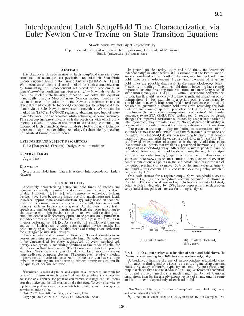
Interdependent Latch Setup/Hold Time Characterization viaEuler-Newton Curve Tracing on State-Transition Equations

Shweta Srivastava and Jaijeet Roychowdhury

Department of Electrical and Computer Engineering, University of MinnesotaEmail: {shwetas,jr}@umn.edu

ABSTRACT

Interdependent characterization of latch setup/hold times is a corecomponent of techniques for pessimism reduction via Setup/HoldInterdependence Aware Static Timing Analysis (SHIA-STA) [1], [2].We present an efficient and novel method for such characterization,by formulating the interdependent setup-hold time problem as anunderdetermined nonlinear equation h(τs,τh) = 0, which we derivefrom the latch’s state-transition function. We solve this equationnumerically using a Moore-Penrose Newton method. Further, weuse null-space information from the Newton’s Jacobian matrix toefficiently find constant-clock-to-Q contours (in the setup/hold timeplane), via an Euler-Newton curve tracing procedure. We validate themethod on TSPC and C2MOS registers, obtaining speedups of morethan 20× over prior approaches while achieving superior accuracy.This speedup increases linearly with the precision with which curvetracing is desired. In view of the importance and large computationalexpense of latch characterization in industry today, the new techniquerepresents a significant enabling technology for dramatically speedingup industrial timing closure flows.

CATEGORIES AND SUBJECT DESCRIPTORS

B.7.2 [Integrated Circuits]: Design Aids – simulation

GENERAL TERMS

Algorithms

KEYWORDS

Setup time, Hold time, Characterization, Interdependence, Euler-Newton

I. INTRODUCTIONAccurately characterizing setup and hold times of latches and

registers is crucially important for static and dynamic timing analysisof digital circuits [1], [3], [4]. With aggressive technology scaling,devices have been becoming faster, but also much more non-ideal;therefore, approximate characterization, typically based on idealiza-tions, are becoming markedly less valid, especially for circuits withmemory such as latches and registers. At the same time, fasterspeeds and smaller design margins make it all the more important tocharacterize with high precision so as to achieve realistic timing cal-culations devoid of unnecessary optimism or pessimism. Optimism insetup/hold times can cause circuit failure, while pessimism results ininferior performance. [1], [5]. As a result, full SPICE-level transientanalysis of latch/register circuits, using detailed device models, hasbeen emerging as the only reliable means of timing characterizationfor cutting-edge industrial designs.

The computational expense of these SPICE-level simulations incurrent industrial practice is extremely high. Setup/hold times needto be characterized for every register/cell of every standard celllibrary, each typically containing hundreds or thousands of cells, forall process-voltage-temperature (PVT) corners or statistical processsamples. Characterization typically takes weeks or months even onlarge dedicated computer clusters. Therefore, even relatively modestimprovements in core characterization procedures can have a largeimpact on reducing the time taken to achieve timing closure and onthe quality of designs achieved.

0Permission to make digital or hard copies of all or part of this work forpersonal or classroom use is granted without fee provided that copies arenot made or distributed for profit or commercial advantage and that copiesbear this notice and the full citation on the first page. To copy otherwise, torepublish, to post on servers or to redistribute to lists, requires prior specificpermission and/or a fee.

DAC 2007, June 4-8, San Diego, California, USA.Copyright 2007 ACM 978-1-59593-627-1/07/0006 ...$5.00.

In general practice today, setup and hold times are determinedindependently; in other words, it is assumed that the two quantitiesare not correlated with each other. However, in actual fact, setup andhold times are interdependent [1]; i.e., multiple pairs of setup andhold times are possible that result in the same clock-to-Q delay1.Flexibility in trading off setup vs hold time is becoming increasinglyimportant for circumventing hold violations and improving slack instatic timing analysis (STA) [1], [2] without sacrificing performance;further, this flexibility is expected to have significant impact on poweroptimization [2]. For example, if a certain path is constrained bya hold violation, exploiting setup/hold interdependence can make itpossible to guarantee a shorter hold time (thus removing the holdviolation and avoiding spurious prediction of failure) at the expenseof a longer (but non-critical) setup time. Such setup/hold interde-pendence aware STA (SHIA-STA) techniques [2] require no circuitchanges for improved performance; rather, by deeper exploitation oflatch dynamics, they provide an extra, “free”, degree of flexibility indesign, of considerable interest for power/performance optimization.

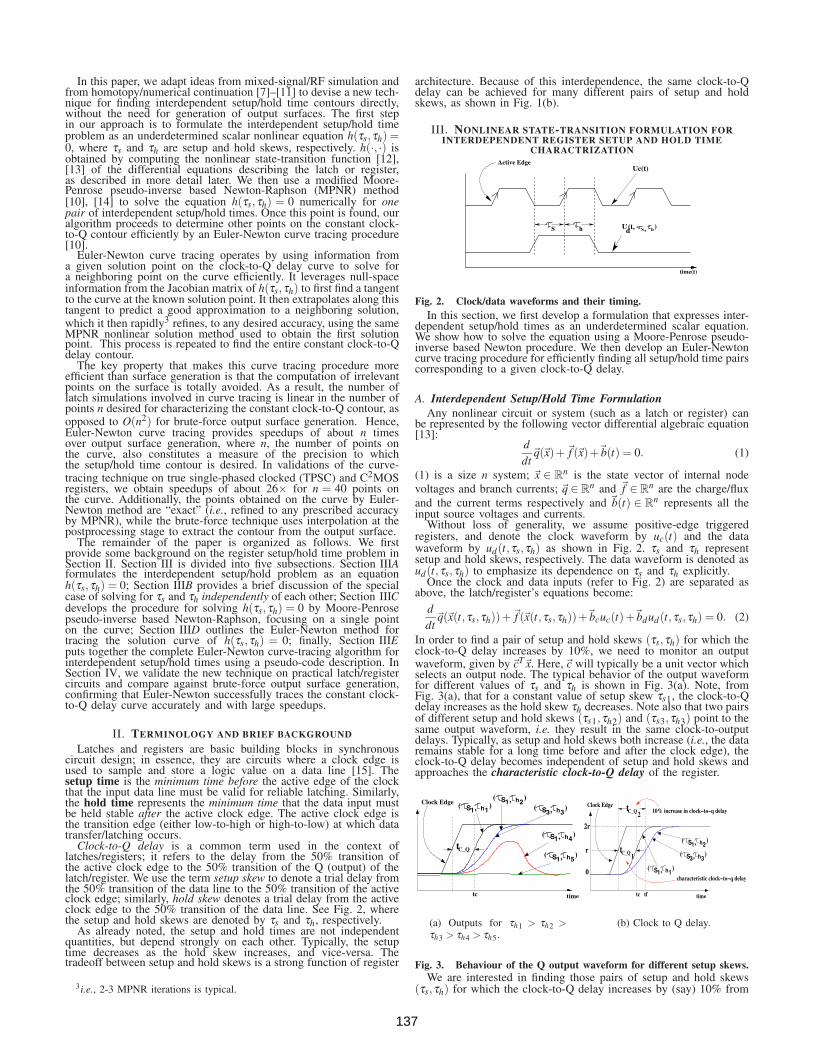
The prevalent technique today for finding interdependent pairs ofsetup/hold times is to first obtain (using many transient simulations ofthe latch) the clock-to-Q delays corresponding to many trial combi-nations of setup and hold skews, i.e., a clock-to-Q delay surface. Thisis followed by extraction of a contour in the setup/hold time planethat contains all points that result in a prescribed increase (e.g., 10%is typical) in clock-to-Q delay. Alternatively, interdependent pairs ofsetup/hold times can be found by determining the register’s outputlevel at a particular time t f

2, again for many trial combinations ofsetup and hold skews, to obtain a surface. This is again followed bycontour extraction; all points in the setup/hold time plane for whichthe output reaches (for example) 50% of the final value at time t fare found – this contour has a constant clock-to-Q delay which isdegraded by 10%.

One such surface for a register output Q vs setup/hold skews isshown in Fig. 1(a); the setup/hold contour obtained is shown inFig. 1(b). The contour shown in Fig. 1(b) has a constant clock-to-Qdelay which is degraded by 10%, hence represents interdependentsetup-hold times pairs of interest for timing analysis.

100200

300400

100

150

200

0

0.5

1

1.5

2

2.5

Setup skew(ps)hold skew (ps)

outp

ut (

V)

(a) Q output surface.

S

h

hold

ske

w

setup skew

(b) Constant clock-to-Qdelay curve.

Fig. 1. (a) Q output surface as a function of setup and hold skews. (b)Contour corresponding to a 10% increase in clock-to-Q delay.

A bottleneck limiting the use of interdependent setup/hold timeinformation in timing analysis flows is the cost of generating constantclock-to-Q delay contours, typically obtained by post-processingoutput surfaces like the one shown in Fig. 1(a). Automated generationof output surfaces involves a much larger number of transientsimulations than for the already expensive task of characterizing setupand hold times independently of each other [6].

1See Section II for an explanation of setup/hold times, clock-to-Q delayand other relevant concepts.

2t f is the time at which clock-to-Q delay increases by (for example) 10%.

136

9.1

In this paper, we adapt ideas from mixed-signal/RF simulation andfrom homotopy/numerical continuation [7]–[11] to devise a new tech-nique for finding interdependent setup/hold time contours directly,without the need for generation of output surfaces. The first stepin our approach is to formulate the interdependent setup/hold timeproblem as an underdetermined scalar nonlinear equation h(τs,τh) =0, where τs and τh are setup and hold skews, respectively. h(·, ·) isobtained by computing the nonlinear state-transition function [12],[13] of the differential equations describing the latch or register,as described in more detail later. We then use a modified Moore-Penrose pseudo-inverse based Newton-Raphson (MPNR) method[10], [14] to solve the equation h(τs,τh) = 0 numerically for onepair of interdependent setup/hold times. Once this point is found, ouralgorithm proceeds to determine other points on the constant clock-to-Q contour efficiently by an Euler-Newton curve tracing procedure[10].

Euler-Newton curve tracing operates by using information froma given solution point on the clock-to-Q delay curve to solve fora neighboring point on the curve efficiently. It leverages null-spaceinformation from the Jacobian matrix of h(τs,τh) to first find a tangentto the curve at the known solution point. It then extrapolates along thistangent to predict a good approximation to a neighboring solution,which it then rapidly3 refines, to any desired accuracy, using the sameMPNR nonlinear solution method used to obtain the first solutionpoint. This process is repeated to find the entire constant clock-to-Qdelay contour.

The key property that makes this curve tracing procedure moreefficient than surface generation is that the computation of irrelevantpoints on the surface is totally avoided. As a result, the number oflatch simulations involved in curve tracing is linear in the number ofpoints n desired for characterizing the constant clock-to-Q contour, asopposed to O(n2) for brute-force output surface generation. Hence,Euler-Newton curve tracing provides speedups of about n timesover output surface generation, where n, the number of points onthe curve, also constitutes a measure of the precision to whichthe setup/hold time contour is desired. In validations of the curve-tracing technique on true single-phased clocked (TPSC) and C2MOSregisters, we obtain speedups of about 26× for n = 40 points onthe curve. Additionally, the points obtained on the curve by Euler-Newton method are “exact” (i.e., refined to any prescribed accuracyby MPNR), while the brute-force technique uses interpolation at thepostprocessing stage to extract the contour from the output surface.

The remainder of the paper is organized as follows. We firstprovide some background on the register setup/hold time problem inSection II. Section III is divided into five subsections. Section IIIAformulates the interdependent setup/hold problem as an equationh(τs,τh) = 0; Section IIIB provides a brief discussion of the specialcase of solving for τs and τh independently of each other; Section IIICdevelops the procedure for solving h(τs,τh) = 0 by Moore-Penrosepseudo-inverse based Newton-Raphson, focusing on a single pointon the curve; Section IIID outlines the Euler-Newton method fortracing the solution curve of h(τs,τh) = 0; finally, Section IIIEputs together the complete Euler-Newton curve-tracing algorithm forinterdependent setup/hold times using a pseudo-code description. InSection IV, we validate the new technique on practical latch/registercircuits and compare against brute-force output surface generation,confirming that Euler-Newton successfully traces the constant clock-to-Q delay curve accurately and with large speedups.

II. TERMINOLOGY AND BRIEF BACKGROUND

Latches and registers are basic building blocks in synchronouscircuit design; in essence, they are circuits where a clock edge isused to sample and store a logic value on a data line [15]. Thesetup time is the minimum time before the active edge of the clockthat the input data line must be valid for reliable latching. Similarly,the hold time represents the minimum time that the data input mustbe held stable after the active clock edge. The active clock edge isthe transition edge (either low-to-high or high-to-low) at which datatransfer/latching occurs.

Clock-to-Q delay is a common term used in the context oflatches/registers; it refers to the delay from the 50% transition ofthe active clock edge to the 50% transition of the Q (output) of thelatch/register. We use the term setup skew to denote a trial delay fromthe 50% transition of the data line to the 50% transition of the activeclock edge; similarly, hold skew denotes a trial delay from the activeclock edge to the 50% transition of the data line. See Fig. 2, wherethe setup and hold skews are denoted by τs and τh, respectively.

As already noted, the setup and hold times are not independentquantities, but depend strongly on each other. Typically, the setuptime decreases as the hold skew increases, and vice-versa. Thetradeoff between setup and hold skews is a strong function of register

3i.e., 2-3 MPNR iterations is typical.

architecture. Because of this interdependence, the same clock-to-Qdelay can be achieved for many different pairs of setup and holdskews, as shown in Fig. 1(b).

III. NONLINEAR STATE-TRANSITION FORMULATION FORINTERDEPENDENT REGISTER SETUP AND HOLD TIME

CHARACTRIZATION

hS h

Active Edge

time(t)

Uc(t)

U )(t, ,S d

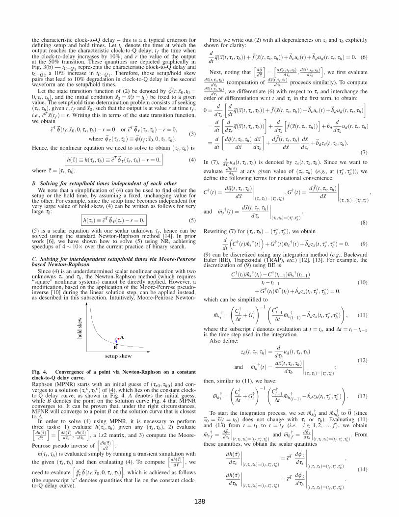
Fig. 2. Clock/data waveforms and their timing.In this section, we first develop a formulation that expresses inter-

dependent setup/hold times as an underdetermined scalar equation.We show how to solve the equation using a Moore-Penrose pseudo-inverse based Newton procedure. We then develop an Euler-Newtoncurve tracing procedure for efficiently finding all setup/hold time pairscorresponding to a given clock-to-Q delay.

A. Interdependent Setup/Hold Time FormulationAny nonlinear circuit or system (such as a latch or register) can

be represented by the following vector differential algebraic equation[13]:

ddt

�q(�x)+�f (�x)+�b(t) = 0. (1)

(1) is a size n system; �x ∈ Rn is the state vector of internal node

voltages and branch currents; �q ∈ Rn and �f ∈ R

n are the charge/fluxand the current terms respectively and �b(t) ∈ R

n represents all theinput source voltages and currents.

Without loss of generality, we assume positive-edge triggeredregisters, and denote the clock waveform by uc(t) and the datawaveform by ud(t,τs,τh) as shown in Fig. 2. τs and τh representsetup and hold skews, respectively. The data waveform is denoted asud(t,τs,τh) to emphasize its dependence on τs and τh explicitly.

Once the clock and data inputs (refer to Fig. 2) are separated asabove, the latch/register’s equations become:

ddt

�q(�x(t,τs,τh))+�f (�x(t,τs,τh))+�bcuc(t)+�bdud(t,τs,τh) = 0. (2)

In order to find a pair of setup and hold skews (τs,τh) for which theclock-to-Q delay increases by 10%, we need to monitor an outputwaveform, given by�cT�x. Here,�c will typically be a unit vector whichselects an output node. The typical behavior of the output waveformfor different values of τs and τh is shown in Fig. 3(a). Note, fromFig. 3(a), that for a constant value of setup skew τs1, the clock-to-Qdelay increases as the hold skew τh decreases. Note also that two pairsof different setup and hold skews (τs1,τh2) and (τs3,τh3) point to thesame output waveform, i.e. they result in the same clock-to-outputdelays. Typically, as setup and hold skews both increase (i.e., the dataremains stable for a long time before and after the clock edge), theclock-to-Q delay becomes independent of setup and hold skews andapproaches the characteristic clock-to-Q delay of the register.

C_Qt

S h1( )

1,S h

S h

S h

S h

Clock Edge

time

,( )2

,( )3 3

,( )

,

1 4

( )1 5

1

tc

(a) Outputs for τh1 > τh2 >τh3 > τh4 > τh5.

S h1( )

1,

S h,( )3 3

h,(21S )

C_Qt

C_Qt

Clock Edge

2

time

2r

r

0

tc

1

tf

10% increase in clock−to−q delay

characteristic clock−to−q delay

(b) Clock to Q delay.

Fig. 3. Behaviour of the Q output waveform for different setup skews.We are interested in finding those pairs of setup and hold skews

(τs,τh) for which the clock-to-Q delay increases by (say) 10% from

137

the characteristic clock-to-Q delay – this is a a typical criterion fordefining setup and hold times. Let tc denote the time at which theoutput reaches the characteristic clock-to-Q delay; t f the time whenthe clock-to-delay increases by 10%; and r the value of the outputat the 50% transition. These quantities are depicted graphically inFig. 3(b) — tC−Q1 represents the characteristic clock-to-Q delay andtC−Q2 a 10% increase in tC−Q1. Therefore, those setup/hold skewpairs that lead to 10% degradation in clock-to-Q delay in the secondwaveform are the setup/hold times.

Let the state transition function of (2) be denoted by �φ(t;�x0, t0 =0,τs,τh), and the initial condition �x0 =�x(t = t0) be fixed to a givenvalue. The setup/hold time determination problem consists of seeking(τs,τh), given r, t f and�x0, such that the output is at value r at time t f ,i.e., �cT�x(t f ) = r. Writing this in terms of the state transition function,we obtain

�cT�φ(t f ;�x0,0,τs,τh)− r = 0 or �cT�φ τ (τs,τh)− r = 0,

where �φ τ (τs,τh) ≡ �φ(t f ;�x0,0,τs,τh).(3)

Hence, the nonlinear equation we need to solve to obtain (τs,τh) is

h(�τ) ≡ h(τs,τh) ≡�cT�φ τ (τs,τh)− r = 0. (4)

where �τ = [τs,τh].

B. Solving for setup/hold times independent of each otherWe note that a simplification of (4) can be used to find either the

setup or the hold time, by assuming a fixed, unchanging value forthe other. For example, since the setup time becomes independent forvery large value of hold skew, (4) can be written as follows for verylarge τh:

h(τs) ≡�cT�φ τ (τs)− r = 0. (5)

(5) is a scalar equation with one scalar unknown τs, hence can besolved using the standard Newton-Raphson method [14]. In priorwork [6], we have shown how to solve (5) using NR, achievingspeedups of 4 ∼ 10× over the current practice of binary search.

C. Solving for interdependent setup/hold times via Moore-Penrosebased Newton-Raphson

Since (4) is an underdetermined scalar nonlinear equation with twounknowns τs and τh, the Newton-Raphson method (which requires“square” nonlinear systems) cannot be directly applied. However, amodification, based on the application of the Moore-Penrose pseudo-inverse [10] during the linear solution step, can be applied instead,as described in this subsection. Intuitively, Moore-Penrose Newton-

B

A

setup skew

hold

skew

Fig. 4. Convergence of a point via Newton-Raphson on a constantclock-to-Q delay curve.Raphson (MPNR) starts with an initial guess of (τs0,τh0) and con-verges to a solution (τs

c,τhc) of (4), which lies on the constant clock-

to-Q delay curve, as shown in Fig. 4. A denotes the initial guess,while B denotes the point on the solution curve Fig. 4 that MPNRconverges to. It can be proven that, under the right circumstances,MPNR will converge to a point B on the solution curve that is closestto A.

In order to solve (4) using MPNR, it is necessary to performthree tasks: 1) evaluate h(τs,τh) given any (τs,τh), 2) evaluate[

dh(�τ)d�τ

]=

[dh(�τ)

dτs,

dh(�τ)dτh

], a 1x2 matrix, and 3) compute the Moore-

Penrose pseudo inverse of[

dh(�τ)d�τ

].

h(τs,τh) is evaluated simply by running a transient simulation with

the given (τs,τh) and then evaluating (4). To compute[

dh(�τ)d�τ

], we

need to evaluate[

ddτ

�φ(t f ;�x0,0,τs,τh)], which is achieved as follows

(the superscript ‘c’ denotes quantities that lie on the constant clock-to-Q delay curve).

First, we write out (2) with all dependencies on τs and τh explicitlyshown for clarity:

ddt

�q(�x(t,τs,τh))+�f (�x(t,τs,τh))+�bcuc(t)+�bdud(t,τs,τh) = 0. (6)

Next, noting that[

d�φd�τ

]=

[d�x(t,τs,τh)

dτs,

d�x(t,τs,τh)dτh

], we first evaluate

d�x(t,τs,τh)dτs

(computation of d�x(t,τs,τh)dτh

proceeds similarly). To computed�x(t,τs,τh)

dτs, we differentiate (6) with respect to τs and interchange the

order of differentiation w.r.t t and τs in the first term, to obtain:

0 =d

dτs

[ddt

�q(�x(t,τs,τh))+�f (�x(t,τs,τh))+�bcuc(t)+�bdud(t,τs,τh)]

=ddt

[d

dτs�q(�x(t,τs,τh))

]+

ddτs

[�f (�x(t,τs,τh))

]+�bd

ddτs

ud(t,τs,τh)

=ddt

[d�q(t,τs,τh)

d�xd�xdτs

]+

d�f (t,τs,τh)d�x

d�xdτs

+�bdzs(t,τs,τh).

(7)

In (7), ddτs

ud(t,τs,τh) is denoted by zs(t,τs,τh). Since we want to

evaluate dh(�τ)dτs

at any given value of (τs,τh) (e.g., at (τ∗s ,τ∗h )), wedefine the following terms for notational convenience:

C†(t) =d�q(t,τs,τh)

d�x

∣∣∣∣(τs,τh)=(τ∗

s ,τ∗h )

,G†(t) =d�f (t,τs,τh)

d�x

∣∣∣∣∣(τs,τh)=(τ∗

s ,τ∗h )

,

and �ms†(t) =

d�x(t,τs,τh)dτs

∣∣∣∣(τs,τh)=(τ∗

s ,τ∗h )

.

(8)

Rewriting (7) for (τs,τh) = (τ∗s ,τ∗h ), we obtain

ddt

(C†(t)�ms

†(t))

+G†(t)�ms†(t)+�bdzs(t,τ∗s ,τ∗h ) = 0. (9)

(9) can be discretized using any integration method (e.g., BackwardEuler (BE), Trapezoidal (TRAP), etc.) [12], [13]. For example, thediscretization of (9) using BE is

C†(ti)�ms†(ti)−C†(ti−1)�ms

†(ti−1)ti − ti−1

+G†(ti)�m†(ti)+�bdzs(ti,τ∗s ,τ∗h ) = 0,

(10)

which can be simplified to

�ms†i =

(C†

i

∆t+G†

i

)−1 (C†

i−1

∆t�ms

†(i−1) −�bdzs(ti,τ∗s ,τ∗h )

), (11)

where the subscript i denotes evaluation at t = ti, and ∆t = ti − ti−1is the time step used in the integration.

Also define:

zh(t,τs,τh) =d

dτhud(t,τs,τh)

and �mh†(t) =

d�x(t,τs,τh)dτh

∣∣∣∣(τs,τh)=(τ∗

s ,τ∗h )

;(12)

then, similar to (11), we have:

�mh†i =

(C†

i

∆t+G†

i

)−1 (C†

i−1

∆t�mh

†(i−1) −�bdzh(ti,τ∗s ,τ∗h )

). (13)

To start the integration process, we set �ms†0 and �mh

†0 to �0 (since

�x0 = �x(t = t0) does not change with τs or τh). Evaluating (11)and (13) from t = t1 to t = t f (i.e. i ∈ 1,2, . . . , f ), we obtain

�ms†f = d�φ τ

dτs

∣∣∣(t,τs,τh)=(t f ,τ∗

s ,τ∗h )

and �mh†f = d�φ τ

dτh

∣∣∣(t,τs,τh)=(t f ,τ∗

s ,τ∗h )

. From

these quantities, we obtain the scalar quantities

dh(�τ)dτs

∣∣∣∣(t,τs,τh)=(t f ,τ∗

s ,τ∗h )

=�cT d�φ τdτs

∣∣∣∣∣(t,τs,τh)=(t f ,τ∗

s ,τ∗h )

,

dh(�τ)dτh

∣∣∣∣(t,τs,τh)=(t f ,τ∗

s ,τ∗h )

=�cT d�φ τdτh

∣∣∣∣∣(t,τs,τh)=(t f ,τ∗

s ,τ∗h )

.

(14)

138

Finally, denoting the matrix[

dh(�τ)d�τ

]by H(�τ), its Moore-Penrose

pseudo-inverse [10] can be expressed as

H(�τ)+∣∣(τs,τh)=(τ∗

s ,τ∗h ) = H(�τ)t (H(�τ)H(�τ)t)−1

∣∣∣(τs,τh)=(τ∗

s ,τ∗h )

, (15)

where H(�τ)+ and H(�τ)t represent the pseudo inverse and transposeof the matrix H(�τ), respectively. These quantities are used for theMPNR-based curve tracing algorithm described in subsection E.

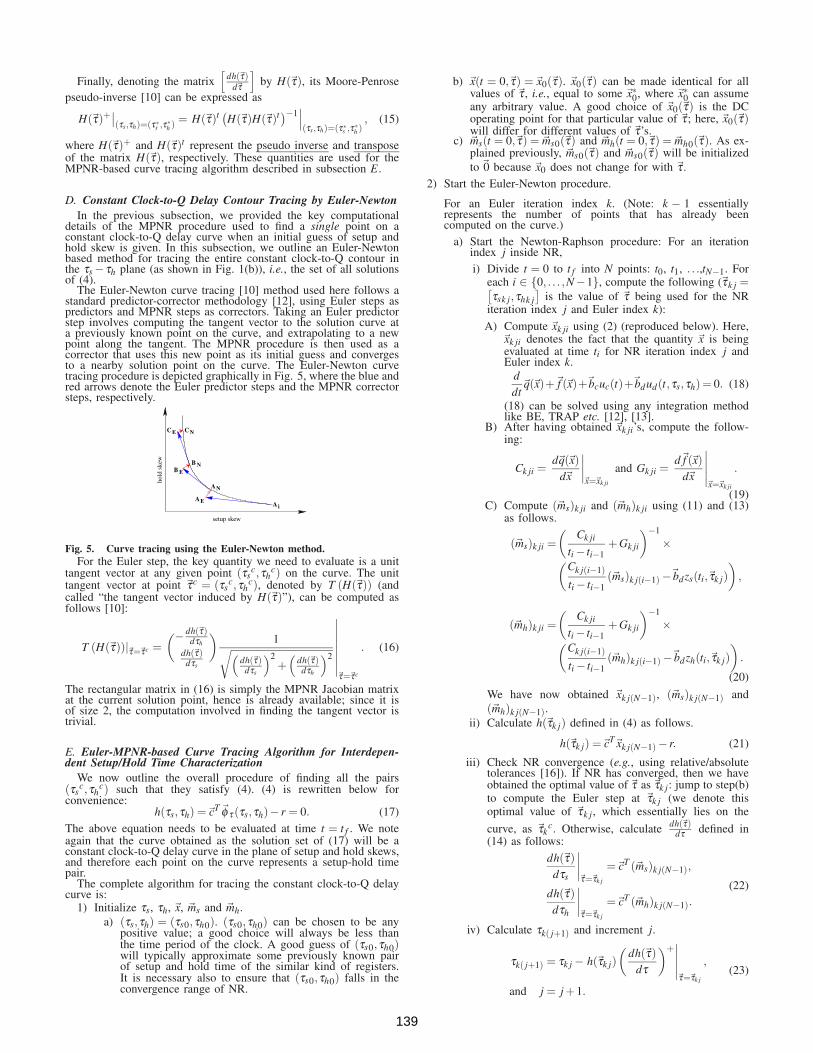
D. Constant Clock-to-Q Delay Contour Tracing by Euler-NewtonIn the previous subsection, we provided the key computational

details of the MPNR procedure used to find a single point on aconstant clock-to-Q delay curve when an initial guess of setup andhold skew is given. In this subsection, we outline an Euler-Newtonbased method for tracing the entire constant clock-to-Q contour inthe τs −τh plane (as shown in Fig. 1(b)), i.e., the set of all solutionsof (4).

The Euler-Newton curve tracing [10] method used here follows astandard predictor-corrector methodology [12], using Euler steps aspredictors and MPNR steps as correctors. Taking an Euler predictorstep involves computing the tangent vector to the solution curve ata previously known point on the curve, and extrapolating to a newpoint along the tangent. The MPNR procedure is then used as acorrector that uses this new point as its initial guess and convergesto a nearby solution point on the curve. The Euler-Newton curvetracing procedure is depicted graphically in Fig. 5, where the blue andred arrows denote the Euler predictor steps and the MPNR correctorsteps, respectively.

AE

EC

Ai

AN

EBB N

NC

setup skew

hold

ske

w

Fig. 5. Curve tracing using the Euler-Newton method.For the Euler step, the key quantity we need to evaluate is a unit

tangent vector at any given point (τsc,τh

c) on the curve. The unittangent vector at point �τc = (τs

c,τhc), denoted by T (H(�τ)) (and

called “the tangent vector induced by H(�τ)”), can be computed asfollows [10]:

T (H(�τ))|�τ=�τc =(− dh(�τ)

dτh

dh(�τ)dτs

)1√(

dh(�τ)dτs

)2+

(dh(�τ)dτh

)2

∣∣∣∣∣∣∣∣�τ=�τc

. (16)

The rectangular matrix in (16) is simply the MPNR Jacobian matrixat the current solution point, hence is already available; since it isof size 2, the computation involved in finding the tangent vector istrivial.

E. Euler-MPNR-based Curve Tracing Algorithm for Interdepen-dent Setup/Hold Time Characterization

We now outline the overall procedure of finding all the pairs(τs

c,τhc) such that they satisfy (4). (4) is rewritten below for

convenience:h(τs,τh) =�cT�φ τ (τs,τh)− r = 0. (17)

The above equation needs to be evaluated at time t = t f . We noteagain that the curve obtained as the solution set of (17) will be aconstant clock-to-Q delay curve in the plane of setup and hold skews,and therefore each point on the curve represents a setup-hold timepair.

The complete algorithm for tracing the constant clock-to-Q delaycurve is:

1) Initialize τs, τh, �x, �ms and �mh.a) (τs,τh) = (τs0,τh0). (τs0,τh0) can be chosen to be any

positive value; a good choice will always be less thanthe time period of the clock. A good guess of (τs0,τh0)will typically approximate some previously known pairof setup and hold time of the similar kind of registers.It is necessary also to ensure that (τs0,τh0) falls in theconvergence range of NR.

b) �x(t = 0,�τ) =�x0(�τ). �x0(�τ) can be made identical for allvalues of �τ , i.e., equal to some �x∗0, where �x∗0 can assumeany arbitrary value. A good choice of �x0(�τ) is the DCoperating point for that particular value of �τ; here, �x0(�τ)will differ for different values of �τ’s.

c) �ms(t = 0,�τ) = �ms0(�τ) and �mh(t = 0,�τ) = �mh0(�τ). As ex-plained previously, �ms0(�τ) and �ms0(�τ) will be initializedto �0 because �x0 does not change for with �τ .

2) Start the Euler-Newton procedure.

For an Euler iteration index k. (Note: k − 1 essentiallyrepresents the number of points that has already beencomputed on the curve.)

a) Start the Newton-Raphson procedure: For an iterationindex j inside NR,i) Divide t = 0 to t f into N points: t0, t1, . . .,tN−1. For

each i ∈ {0, . . . ,N−1}, compute the following (�τk j =[τsk j,τhk j

]is the value of �τ being used for the NR

iteration index j and Euler index k):

A) Compute �xk ji using (2) (reproduced below). Here,�xk ji denotes the fact that the quantity �x is beingevaluated at time ti for NR iteration index j andEuler index k.

ddt

�q(�x)+�f (�x)+�bcuc(t)+�bdud(t,τs,τh) = 0. (18)

(18) can be solved using any integration methodlike BE, TRAP etc. [12], [13].

B) After having obtained �xk ji’s, compute the follow-ing:

Ck ji =d�q(�x)

d�x

∣∣∣∣�x=�xk ji

and Gk ji =d�f (�x)

d�x

∣∣∣∣∣�x=�xk ji

.

(19)C) Compute (�ms)k ji and (�mh)k ji using (11) and (13)

as follows.

(�ms)k ji =(

Ck ji

ti − ti−1+Gk ji

)−1

×(Ck j(i−1)

ti − ti−1(�ms)k j(i−1) −�bdzs(ti,�τk j)

),

(�mh)k ji =(

Ck ji

ti − ti−1+Gk ji

)−1

×(Ck j(i−1)

ti − ti−1(�mh)k j(i−1) −�bdzh(ti,�τk j)

).

(20)

We have now obtained �xk j(N−1), (�ms)k j(N−1) and(�mh)k j(N−1).

ii) Calculate h(�τk j) defined in (4) as follows.

h(�τk j) =�cT�xk j(N−1) − r. (21)

iii) Check NR convergence (e.g., using relative/absolutetolerances [16]). If NR has converged, then we haveobtained the optimal value of �τ as �τk j: jump to step(b)to compute the Euler step at �τk j (we denote thisoptimal value of �τk j , which essentially lies on the

curve, as �τkc. Otherwise, calculate dh(�τ)

dτ defined in(14) as follows:

dh(�τ)dτs

∣∣∣∣�τ=�τk j

=�cT (�ms)k j(N−1),

dh(�τ)dτh

∣∣∣∣�τ=�τk j

=�cT (�mh)k j(N−1).

(22)

iv) Calculate τk( j+1) and increment j.

τk( j+1) = τk j − h(�τk j)(

dh(�τ)dτ

)+∣∣∣∣∣�τ=�τk j

,

and j = j +1.

(23)

139

In (23),(

dh(�τ)dτ

)+is the Moore-Penrose pseudo-

inverse of dh(�τ)dτ , which can be calculated using (15)

as(dh(�τ)

dτ

)+=

(dh(�τ)

dτ

)t [dh(�τ)dτ

(dh(�τ)

dτ

)t]−1

,

(24)

where(

dh(�τ)dτ

)tis the transpose of dh(�τ)

dτ . Go to step(i) for the next iteration of NR.

b) Compute the tangent unit vector induced by dh(�τ)d�τ using

(16) for �τ =�τkc as follows:

T

(dh(�τ)

dτ

)=

(− dh(�τ)dτh

dh(�τ)dτs

)1√(

dh(�τ)dτs

)2+

(dh(�τ)dτh

)2(25)

c) Compute a new pair of (τs0,τh0) along the unit tangentvector (the predictor step):

�τ(k+1)0 =�τkc + α .T

(dh(�τ)

dτ

)∣∣∣∣�τ=�τk

c,

and k = k +1.

(26)

α is a step length along the tangent direction. Go to step(a) of the Euler-Newton procedure; repeat until the curveis traversed to any desired extent.

IV. VALIDATION USING TSPC AND C2MOS REGISTERS

In this section, we validate the interdependent setup/hold timecharacterization algorithm developed above using two types ofregisters: a TPSC register and a C2MOS positive edge triggeredmaster/slave register. We describe the validation procedure in detailbelow. Our results, which we compare against brute-force outputsurface generation, confirm that the new curve-tracing method findsconstant clock-to-Q contours accurately, and with computation linearin the number of contour points desired. We obtain speedups ofabout 26× over surface generation4 for 40 curve points (representingexcellent precision for timing analysis purposes). Additionally, wehave chosen reltol/abstol for MPNR such that the points obtained onthe curve are accurate up to 5 digits.

A. True single-phased clocked register

CLK

Vdd

CLK

CLK

Vdd Vdd Vdd

CLK

D Q

Fig. 6. Positive edge-triggered register in TSPC.The positive edge triggered true single-phased clocked register

shown in Fig. 6 features positive setup and hold time constraints.The clock waveform uc(t) used in the register has a period of 10ns,with logic 0 at 0V and logic 1 at 2.5V . The clock input has an initialdelay of 1ns; rise/fall times are both 0.1ns. Therefore, its active clockedges are located at 1ns, 11ns, 21ns, etc.. The chosen data waveformud(t,τs,τh) is centered around the active clock edge which starts at11ns. The data waveform changes its shape (variable pulse width,refer to Fig. 2) depending on the values of τs and τh.

At first, to determine the characteristic clock-to-Q delay, theregister is simulated for large values of τs and τh and the outputis monitored. The output waveform reaches 1.25V (50% of its finalvalue) at tc = 11.348ns, hence the characteristic clock-to-Q delayequals 298ps (the distance from the 50% active clock transition tothe 50% transition of the output). Here, we use a standard definitionfor setup and hold times: that they lead to an increase of 10% over

4Speedup numbers are obtained via apples-to-apples comparisons on anAMD Athlon64 3000+ based PC, with 512MB RAM, running Linux kernel2.6.12. All algorithms are implemented in a MATLAB/C/C++ simulationprototyping environment.

the characteristic clock-to-Q delay. Hence the constant clock-to-Qdelay value for contour generation equals 327.8ps. Accordingly, weset t f = 11ns+ rise−time

2 +327.8ps = 11.3778ns and r = 1.25V in (4)(tc, t f and r used here correspond to the same symbols in Fig. 3(b)).

Determination of the first point on the curve involves starting witha good guess for (τs0,τh0) to seed NR. To find one, we make thehold skew τh0 very large so that the setup time will becomes largelyindependent of hold skew. We start with a setup skew interval[τsL,τsR], where the register latches the data properly for τsL, andfails to latch data for τsR. Hence this interval will contain the setuptime point τs

c. We then narrow down the setup skew interval using acoarse binary search, until the interval length falls in the convergencerange of NR as shown in Fig. 7(b).

0s

Cloc

k−to

−Q D

elay

Setup Skew (tau): sc

10% increase in clock to Q time.

Interval around an estimate of setup time

(a) Setup-time characteri-zation.

0s

Cloc

k−to

−Q D

elay

Range for NRSetup Skew (tau): s

c

10% increase in clock to Q time.

(b) Convergence region forMPNR.

Fig. 7. (a) Setup time characterization by running binary search withinan interval bracketing the setup time. (b) Convergence region of MPNRin an interval around the estimate of setup time.

Either τsL or τsR can be used as the initial guess τs0 for MPNRsolution. Then, we start the Euler-Newton process as outlined previ-ously. MPNR typically converges very quickly (2–3 iterations) as thecurve is traced since the Euler steps provide excellent initial guesses.The constant clock-to-Q delay contour obtained by the procedure isshown in Fig. 8. To verify the correctness of this curve, we also

150 200 250 300 350100

120

140

160

180

200

setup skew (ps)

hold

ske

w (

ps)

Fig. 8. Constant clock-to-Q delay curve obtained by the Euler-Newtonmethod. Curve represents the pairs of setup and hold skews whichincreases the characteristic clock-to-Q delay by 10%.extract the 10% degraded constant clock-to-Q delay curve for thisregister using the brute-force output surface generation technique. Anoutput surface is generated at time t f = 11.778ns by independentlyvarying setup and hold skews as shown in Fig. 9. A plane at a“height” of 1.25V is then drawn to obtain the intersection contourof the output surface. This intersection curve represents the set ofall hold-setup skew pairs which results in 10% increase in clock-to-Q delay. The top view of the curve obtained by this intersection

Fig. 9. Q output surface as a function of independent setup and holdskews.procedure is shown in Fig. 10. The contour from Euler-Newton curve

140

tracing (Fig. 8) is overlaid on the intersection of the plane and theoutput surface in Fig. 10. It is apparent from Fig. 10 that the curveobtained by Euler-Newton methodology exactly matches the constantclock-to-Q delay curve obtained from the surface, thereby verifyingthe correctness of the new method.

Fig. 10. Top view of intersection curve of plane and output surface andthe superimposition of curve obtained by Euler-Newton method

In our implementation, Euler-Newton curve tracing took 45 min-utes to trace 40 points on the contour, while brute-force output surfacegeneration consumed 20 hours (for 40×40 simulations) to obtain 40points on the curve; representing a speedup of about 26×.

B. C2MOS positive-edge triggered master-slave register

CLK

CLK

CLK

CLK

VddVdd

D X Q

(a) Register.

50%

80%

Failed Transition

Successful Transition

(b) Output waveforms.

Fig. 11. (a) C2MOS positive-edge triggered master-slave register. (b)Output waveform fails to complete the transition even after reaching80% of its true value.

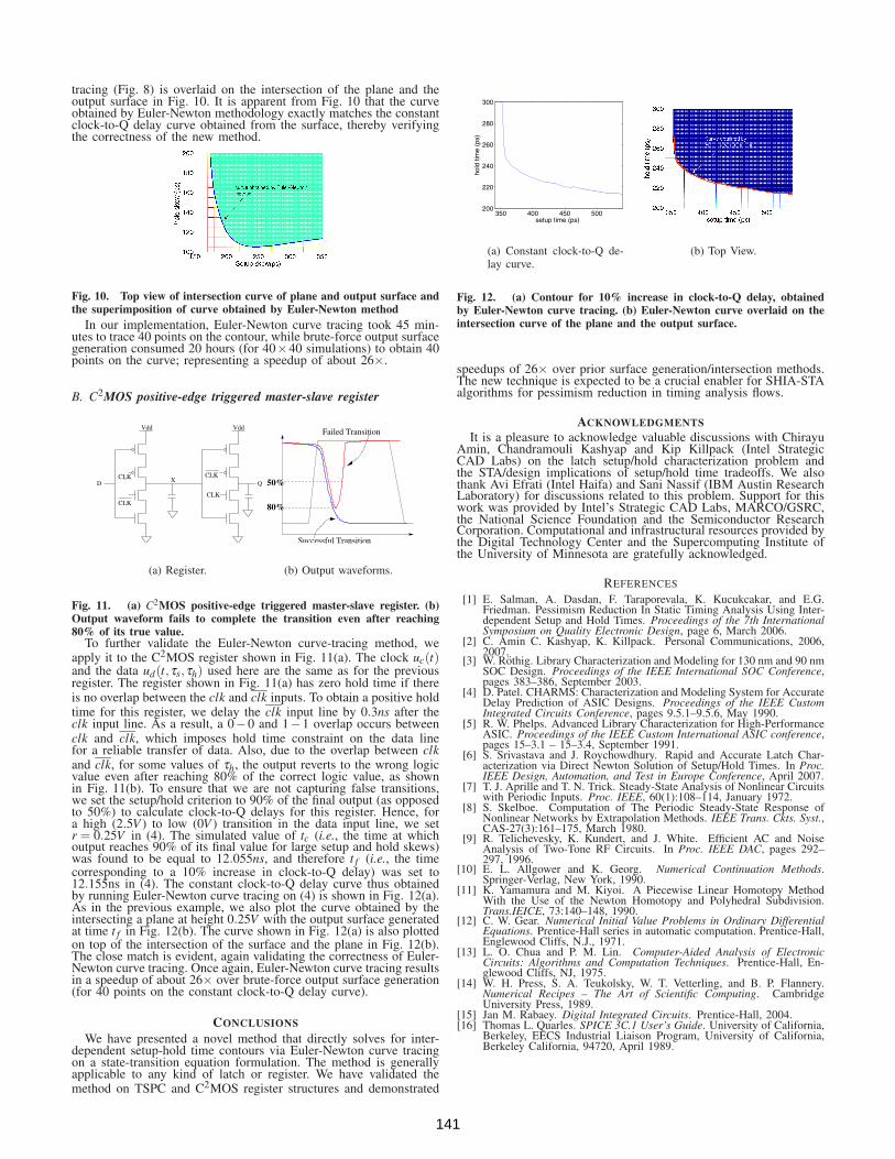
To further validate the Euler-Newton curve-tracing method, weapply it to the C2MOS register shown in Fig. 11(a). The clock uc(t)and the data ud(t,τs,τh) used here are the same as for the previousregister. The register shown in Fig. 11(a) has zero hold time if thereis no overlap between the clk and clk inputs. To obtain a positive holdtime for this register, we delay the clk input line by 0.3ns after theclk input line. As a result, a 0−0 and 1−1 overlap occurs betweenclk and clk, which imposes hold time constraint on the data linefor a reliable transfer of data. Also, due to the overlap between clkand clk, for some values of τh, the output reverts to the wrong logicvalue even after reaching 80% of the correct logic value, as shownin Fig. 11(b). To ensure that we are not capturing false transitions,we set the setup/hold criterion to 90% of the final output (as opposedto 50%) to calculate clock-to-Q delays for this register. Hence, fora high (2.5V ) to low (0V ) transition in the data input line, we setr = 0.25V in (4). The simulated value of tc (i.e., the time at whichoutput reaches 90% of its final value for large setup and hold skews)was found to be equal to 12.055ns, and therefore t f (i.e., the timecorresponding to a 10% increase in clock-to-Q delay) was set to12.155ns in (4). The constant clock-to-Q delay curve thus obtainedby running Euler-Newton curve tracing on (4) is shown in Fig. 12(a).As in the previous example, we also plot the curve obtained by theintersecting a plane at height 0.25V with the output surface generatedat time t f in Fig. 12(b). The curve shown in Fig. 12(a) is also plottedon top of the intersection of the surface and the plane in Fig. 12(b).The close match is evident, again validating the correctness of Euler-Newton curve tracing. Once again, Euler-Newton curve tracing resultsin a speedup of about 26× over brute-force output surface generation(for 40 points on the constant clock-to-Q delay curve).

CONCLUSIONS

We have presented a novel method that directly solves for inter-dependent setup-hold time contours via Euler-Newton curve tracingon a state-transition equation formulation. The method is generallyapplicable to any kind of latch or register. We have validated themethod on TSPC and C2MOS register structures and demonstrated

350 400 450 500200

220

240

260

280

300

setup time (ps)

hold

tim

e (p

s)

(a) Constant clock-to-Q de-lay curve.

(b) Top View.

Fig. 12. (a) Contour for 10% increase in clock-to-Q delay, obtainedby Euler-Newton curve tracing. (b) Euler-Newton curve overlaid on theintersection curve of the plane and the output surface.

speedups of 26× over prior surface generation/intersection methods.The new technique is expected to be a crucial enabler for SHIA-STAalgorithms for pessimism reduction in timing analysis flows.

ACKNOWLEDGMENTSIt is a pleasure to acknowledge valuable discussions with Chirayu

Amin, Chandramouli Kashyap and Kip Killpack (Intel StrategicCAD Labs) on the latch setup/hold characterization problem andthe STA/design implications of setup/hold time tradeoffs. We alsothank Avi Efrati (Intel Haifa) and Sani Nassif (IBM Austin ResearchLaboratory) for discussions related to this problem. Support for thiswork was provided by Intel’s Strategic CAD Labs, MARCO/GSRC,the National Science Foundation and the Semiconductor ResearchCorporation. Computational and infrastructural resources provided bythe Digital Technology Center and the Supercomputing Institute ofthe University of Minnesota are gratefully acknowledged.

REFERENCES

[1] E. Salman, A. Dasdan, F. Taraporevala, K. Kucukcakar, and E.G.Friedman. Pessimism Reduction In Static Timing Analysis Using Inter-dependent Setup and Hold Times. Proceedings of the 7th InternationalSymposium on Quality Electronic Design, page 6, March 2006.

[2] C. Amin C. Kashyap, K. Killpack. Personal Communications, 2006,2007.

[3] W. Rothig. Library Characterization and Modeling for 130 nm and 90 nmSOC Design. Proceedings of the IEEE International SOC Conference,pages 383–386, September 2003.

[4] D. Patel. CHARMS: Characterization and Modeling System for AccurateDelay Prediction of ASIC Designs. Proceedings of the IEEE CustomIntegrated Circuits Conference, pages 9.5.1–9.5.6, May 1990.

[5] R. W. Phelps. Advanced Library Characterization for High-PerformanceASIC. Proceedings of the IEEE Custom International ASIC conference,pages 15–3.1 – 15–3.4, September 1991.

[6] S. Srivastava and J. Roychowdhury. Rapid and Accurate Latch Char-acterization via Direct Newton Solution of Setup/Hold Times. In Proc.IEEE Design, Automation, and Test in Europe Conference, April 2007.

[7] T. J. Aprille and T. N. Trick. Steady-State Analysis of Nonlinear Circuitswith Periodic Inputs. Proc. IEEE, 60(1):108–114, January 1972.

[8] S. Skelboe. Computation of The Periodic Steady-State Response ofNonlinear Networks by Extrapolation Methods. IEEE Trans. Ckts. Syst.,CAS-27(3):161–175, March 1980.

[9] R. Telichevesky, K. Kundert, and J. White. Efficient AC and NoiseAnalysis of Two-Tone RF Circuits. In Proc. IEEE DAC, pages 292–297, 1996.

[10] E. L. Allgower and K. Georg. Numerical Continuation Methods.Springer-Verlag, New York, 1990.

[11] K. Yamamura and M. Kiyoi. A Piecewise Linear Homotopy MethodWith the Use of the Newton Homotopy and Polyhedral Subdivision.Trans.IEICE, 73:140–148, 1990.

[12] C. W. Gear. Numerical Initial Value Problems in Ordinary DifferentialEquations. Prentice-Hall series in automatic computation. Prentice-Hall,Englewood Cliffs, N.J., 1971.

[13] L. O. Chua and P. M. Lin. Computer-Aided Analysis of ElectronicCircuits: Algorithms and Computation Techniques. Prentice-Hall, En-glewood Cliffs, NJ, 1975.

[14] W. H. Press, S. A. Teukolsky, W. T. Vetterling, and B. P. Flannery.Numerical Recipes – The Art of Scientific Computing. CambridgeUniversity Press, 1989.

[15] Jan M. Rabaey. Digital Integrated Circuits. Prentice-Hall, 2004.[16] Thomas L. Quarles. SPICE 3C.1 User’s Guide. University of California,

Berkeley, EECS Industrial Liaison Program, University of California,Berkeley California, 94720, April 1989.

141