Interdependent Preference Modelsas a Theory of Intentions†

Faruk Gul

and

Wolfgang Pesendorfer

Princeton University

July 2010

Abstract

We provide a preference framework for situations in which “intentions matter.” A

behavioral type describes the individual’s observable characteristics and the individual’s

personality. We define a canonical behavioral type space and provide a condition that

identifies collections of behavioral types that are equivalent to components of the canonical

type space. We also develop a reciprocity model within our framework and show how it

enables us to distinguish between strategic (or instrumental) generosity and true generosity.

† This research was supported by grants SES9911177, SES0236882, SES9905178 and SES0214050 fromthe National Science Foundation. We thank Stephen Morris and Phil Reny for their comments.

1. Introduction

In many economic settings, knowing the physical consequences of the interaction is

not enough to determine its utility consequences. For example, Blount (1995) observes

that experimental subjects may reject an unfair division when another subject willingly

proposes it and yet might accept it when the other subject is forced to propose it. Hence,

individuals care not just about physical consequences but also about the intentions of those

around them. In this paper, we develop a framework for modeling intentions and how they

affect others’ behavior.

We call our descriptions of intentions interdependent preference models (IPMs). In an

IPM, a person’s ranking of social outcomes depends on the characteristics and personal-

ities of those around him. Characteristics are attributes such as the individual’s wealth,

education or gender. Personalities describe how preferences respond to the characteristics

and personalities of others. Thus, the personality defines a person’s altruism, his desire

to conform, his willingness to reciprocate or his inclination to be spiteful. To understand

how our theory works, consider the following example.

Two individuals are to share a fixed sum of money. There are three possible outcomes:

the sum of money can be given to one or the other person or it can be shared equally.

There are two possible preferences for each player; either the player is selfish (S) and ranks

getting the whole sum above sharing it equally or the player is generous (G) and ranks

sharing the sum above getting it all. Giving the whole sum to the opponent is always the

least preferred outcome.

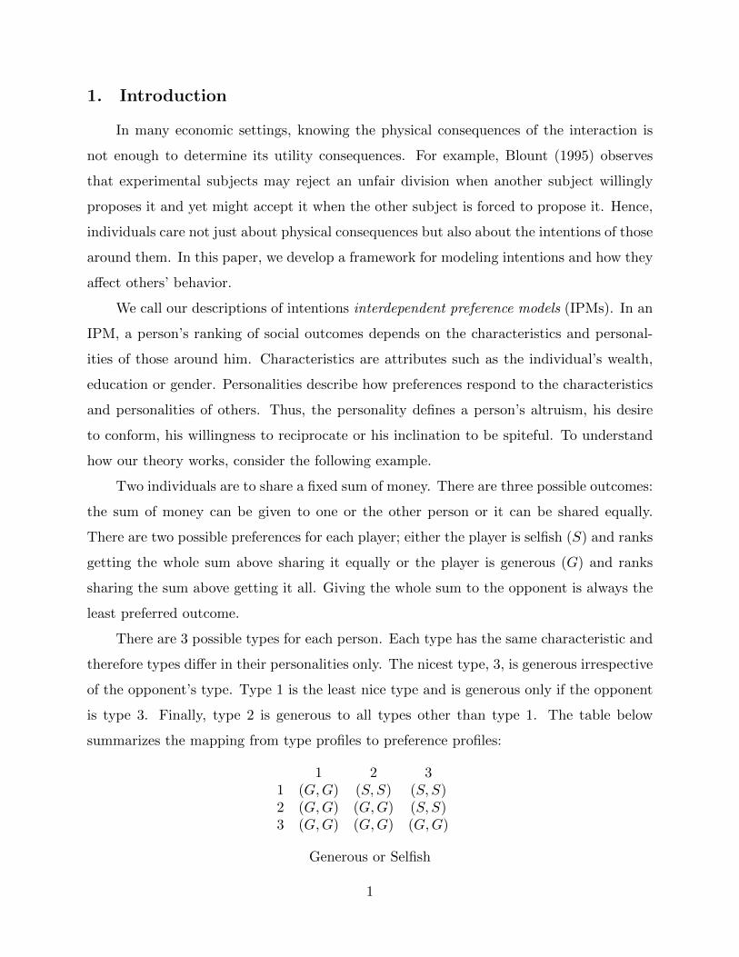
There are 3 possible types for each person. Each type has the same characteristic and

therefore types differ in their personalities only. The nicest type, 3, is generous irrespective

of the opponent’s type. Type 1 is the least nice type and is generous only if the opponent

is type 3. Finally, type 2 is generous to all types other than type 1. The table below

summarizes the mapping from type profiles to preference profiles:

1 2 31 (G,G) (S, S) (S, S)2 (G,G) (G,G) (S, S)3 (G,G) (G,G) (G,G)

Generous or Selfish

1

We call such a table an IPM. Levine (1998) introduces the first example of an IPM

and uses it to address experimental evidence in centipede, ultimatum and public goods

experiments.

Three features of IPMs are noteworthy: first, a type describes relevant personality

attributes rather than information. These attributes determine both the person’s and his

opponent’s preferences over outcomes, not their beliefs over an uncertain state of nature.

To put it another way, IPM’s do not incorporate asymmetric information (or interactive

knowledge); they only model interactive preferences. Each entry in the table describes the

preference the two individuals would have if they knew the other’s type; the IPM does not

address the question whether an individuals knows the others’ type.

Second, an IPM does not describe the available strategic choices; it is not a game. We

can study how Persons I and II above would play many different games. We can also use

this IPM as the preference model for a competitive economy. Hence, IPMs describe only

the preference environment not the institutional setting.

Third, in an IPM, individuals have preferences over physical outcomes and these pref-

erences depend on the persistent personalities and characteristics of everyone involved, not

on observed or predicted behavior or beliefs. Hence, the interaction of these fixed person-

alities determines whether each person is generous or selfish. Whether or not a person acts

selfishly on a given day or believes the other will act selfishly is relevant only to the extent

that these actions affect the physical outcome.

The last two observations highlight the main differences between IPMs and existing

models of reciprocity. In our approach, there is a clear separation between the underly-

ing preference framework (i.e., the IPM) and the particular institution (game, market).

Geanakoplos, Pearce and Stacchetti’s (1989) and the many reciprocity models based on

their approach such as Rabin (1993), Dufwenberg and Kirchsteiger (2004), Falk and Fis-

chbacher (2006), Segal and Sobel (2007) and Battigalli and Dufwenberg (2009), model

preference interactions through a circular definition that permits preferences to depend on

the very behavior (or beliefs about behavior) that they induce.

This circularity enables psychological games to accommodate many departures from

standard theory. Some of these departures fall outside the reach of IPMs. For example,

2

Geanakoplos, Pearce and Stacchetti show how psychological games can model a preference

for being surprised or a preference for pandering to others’ expectations. Such preferences

are best described within the context of the particular interaction and hence are difficult

to model as IPMs.

Because IPMs afford a separation between preferences and institutions they are well

suited for analyzing economic design problems or for comparisons of institutions. Consider,

for example, the (complete information) implementation problem: let f be a social choice

rule (or performance criterion) that associates a set of outcomes with each profile, θ, of

individual attributes. When is it possible to find a game form g such that all equilibrium

outcomes of the game (g, θ) are among the desirable outcomes f(θ) for every θ? Note

that the separation of the preference framework (i.e., the attributes θ) from the game

form is essential for analyzing such a problem. Without this separation, just stating the

implementation problem becomes a formidable task.

More generally, separating preferences from institutions is essential anytime we wish to

evaluate a particular institution or assess a specific environmental factor: does the English

auction Pareto dominate the Dutch auction? Do prohibitions on resale enhance efficiency?

Does greater monitoring increase effort? Questions such as these demand a performance

criterion over consequences that can be expressed without reference to specific institutions.

In an IPM, a type maps the other person’s types to preference profiles. Hence, the

definition of a type is circular. Our first objective is to identify a criterion to determine

when this circularity is problematic and when it is not; that is, to identify when interde-

pendent preference types can be reduced to preference statements. To see how this can

be done, note that in the above example, the preference profile associated with type 3

does not depend on the opponent’s personality and therefore type 3 can describe himself

without any reference to his opponent’s type. But once type 3 is identified, type 2 can

describe himself as a personality that is generous only to the personality that has just

been identified. Finally, type 1 can identify himself as someone who is generous to the two

personalities that have been identified so far and no one else. Hence, in the above exam-

ple, we can eliminate the circularity by restating each type as a hierarchy of preference

statements.

3

We define the canonical type space for interdependent preferences as sequences of such

hierarchical preferences statements. In Theorem 1, we show that each component of the

canonical type space is an IPM. However, not every IPM is part of the canonical type

space. Theorem 2 provides a simple condition on IPMs, (validity) that guarantees that

an IPM is a component of the canonical type space. When a model fails validity, types

cannot be reduced to preference statements. To formalize this observation, we develop a

notion of communicability in a given language. We show that players can communicate

their type in the language of preferences if and only if the model is valid (Theorem 3).

As an application of our model, we define reciprocity and identify a class of valid

interdependent preference models with reciprocating types. To do this, we consider settings

in which preferences can be ranked according to their kindness. That is, we identify each

preference with a real number and interpret higher numbers as kinder preferences. For

example, assume xi is i’s consumption and

V r(x1, x2) = u(x1) + ru(x2)

is the utility that person 1 enjoys if r is his preference. The IPM specifies how types

determine r. Let δ(t, t′) ∈ [r, r] be the preference of type t when the opponent is type

t′. A higher r is a kinder preference. Type t is nicer than type t′ if t is kinder than t′ to

every opponent type; a type reciprocates if it is kinder to a nicer opponent. Hence, if δ

is increasing in the first argument, higher types are kinder. Then, if δ is also increasing

in the second argument, all types reciprocate. In Theorems 4 and 5 we characterize two

simple classes of reciprocity models.

Our canonical type space provides a foundation for valid IPMs that is analogous to

the Mertens and Zamir (1985) and Brandenburger and Dekel (1993) foundations for infor-

mational (Harsanyi) types. In the concluding section, we discuss the relationship between

our results and technically related issues in that literature. In particular, we discuss Berge-

mann and Morris (2009) and the literature on communication and consensus (Geanakoplos

and Polemarchakis (1982), Cave (1983), Bacharach (1985), Parikh and Krasucki (1990)).

All proofs are in the appendix.

4

2. Behavioral Types

We assume that there is one other person whose type affects the decision-maker. The

two-person setting simplifies the notation and the extension to the n-person setting is

straightforward. A set of social outcomes A, a set of characteristics Ω and a collection of

preferences R on A characterizes the environment. For example, a social outcome could

be the quantity of a public good together with a division of its cost or a pair of individual

consumption levels. A characteristic might specify a player’s occupation or education. The

triple (A,R,Ω) describes the underlying economic primitives.

We assume that A and Ω are compact metric spaces and that R is a nonempty and

compact set of continuous preference relations1 on A. An interdependent preference model

(IPM) is a triple M = (T, γ, ω) where T is the type space, γ is a function that assigns a

preference to each pair of types, and ω is a function that identifies the characteristic of

each type.

Definition: Let T be a compact metric space, γ : T × T → R and ω : T → Ω be

continuous functions. Then, M = (T, γ, ω) is an interdependent preference model (IPM).

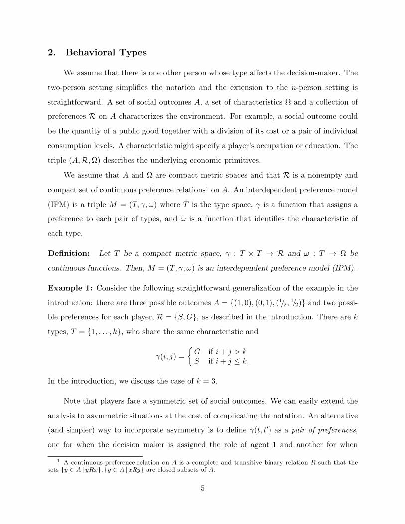
Example 1: Consider the following straightforward generalization of the example in the

introduction: there are three possible outcomes A = (1, 0), (0, 1), (1/2, 1/2) and two possi-

ble preferences for each player, R = S,G, as described in the introduction. There are k

types, T = 1, . . . , k, who share the same characteristic and

γ(i, j) =

G if i+ j > kS if i+ j ≤ k.

In the introduction, we discuss the case of k = 3.

Note that players face a symmetric set of social outcomes. We can easily extend the

analysis to asymmetric situations at the cost of complicating the notation. An alternative

(and simpler) way to incorporate asymmetry is to define γ(t, t′) as a pair of preferences,

one for when the decision maker is assigned the role of agent 1 and another for when

1 A continuous preference relation on A is a complete and transitive binary relation R such that thesets y ∈ A | yRx, y ∈ A |xRy are closed subsets of A.

5

he is assigned the role of agent 2. With this modification, our model can be applied to

asymmetric situations.

For the IPM (T, γ, ω) the type profile (t, t′) implies the preference profile

Γ(t, t′) := (γ(t, t′), γ(t′, t)) (1)

Below, we sometimes refer to an IPM (T,Γ, ω). In that case, it is understood that Γ

satisfies (1) for some γ : T × T → R.

The function γ(t, ·) : T → R describes how the agent’s preference changes as a function

of the opponent’s type. Hence, γ(t, ·) represents an agent’s personality. Note, however,

that the type space T is not a primitive of the economic environment. Therefore, γ(t, ·)cannot serve as a satisfactory definition of an agents’ personality. To be meaningful, a

personality must be expressed in terms of the primitives (A,Ω,R). Next, we describe how

this can be done.

Types are hierarchies of preference statements. In round 0, each type reports a char-

acteristic (the characteristic of the type). In rounds n ≥ 1, each type reports a set of

preference profiles. The preference profile (R,R′) is part of the round n report if, given

the opponent’s report in all previous rounds, it is possible that the player has preference

R and his opponent has preference R′. Theorem 1 shows that when a collection of such

hierarchies satisfies a straightforward consistency condition, it is an IPM.

Before providing the formal definition, it is useful to illustrate the correspondence

between behavioral types and hierarchies of preference statements in Example 1. All types

in this example have the same characteristic and therefore there is nothing to report in

round 0. In round 1, each type reports the set of possible preference profiles given his

type. For types 1, . . . , k − 1, the preference profile is either (G,G) or (S, S). Hence, types

1, . . . , k− 1 can report that both players will have identical preferences and that both the

generous and the selfish preference profile are possible. For type k (the most generous

type) we have k+ t > k for all t. Therefore, the preference profile is (G,G) when any type

is matched with k. Round 1 thus identifies the most generous personality (type k).

In round 2, each type reports two sets of preferences, one in response to the round-1

(opponent’s) report (G,G) and one in response to the round-1 report (G,G), (S, S). In

6

response to (G,G) all types must report (G,G). This follows from a basic consistency

requirement: if a player reports a single possible preference profile (R,R′) in round n, then,

in all successive rounds, his opponent must report (R′, R) (i.e., the same preference profile

with the roles permuted). There are three possible responses to (G,G), (S, S): type k

reports (G,G), types 2, . . . , k − 1 report (G,G), (S, S) and type 1 reports (S, S).Therefore, round 2 identifies type 1 as the least generous personality.

Continuing in this fashion, round 3 identifies the second most generous personality

(type k − 1) and round 4 identifies the second least generous personality (type 2). After

k rounds, such hierarchical preference statements reveal all personalities in Example 1.

Note that agents report preference profiles rather than individual preferences. Individual’s

types place restrictions not only on their own preference but also on the preferences of

their opponents. Hence, to permit the full generality of possible preference interactions, it

is necessary that hierarchical statements convey (sets of) preference profiles not just their

own preferences.2

To define personalities, we use the following notation and definitions. When Xj is

a metric space for all j in some countable or finite index set J , we endow ×j∈JXj with

the sup metric. For any compact metric space X, let HX be the set of all nonempty,

closed subsets of X and endow HX with the Hausdorff topology. For the compact metric

spaces X,Z let C(X,HZ) denote the set of all functions f : X → HZ such that their

graph G(f) = (x, z) ∈ X × Z | z ∈ f(x) is closed in X × Z.3 We endow C(X,HZ) with

the following metric: d(f, g) = dH(G(f), G(g)), where dH is the Hausdorff metric on the

set of all nonempty closed subsets of X × Z. We identify the function f : X → Z with

the function f : X → HZ such that f(x) = f(x) for all x ∈ X. It is easy to verify

that such a function f is an element of C(X,HZ) if and only if f is continuous. We use

C(X,Z) ⊂ C(X,HZ) to denote the set of continuous functions from X to Z.

We letH denoteHR×R, the collection of all closed subsets of preference profiles (closed

subsets of R × R). Types are consistent preference response hierarchies. As illustrated

above, these hierarchies specify sets of preferences that are gradually refined as more

2 In example 1 both agents have the same preference hence statements about agents’ own preferencesare sufficient. However, this is not true in general. To identify certain personality types, it may benecessary to convey information about the opponent’s preference.

3 Hence, C(X,HZ) is the set of upper hemi-continuous correspondences from X to Z.

7

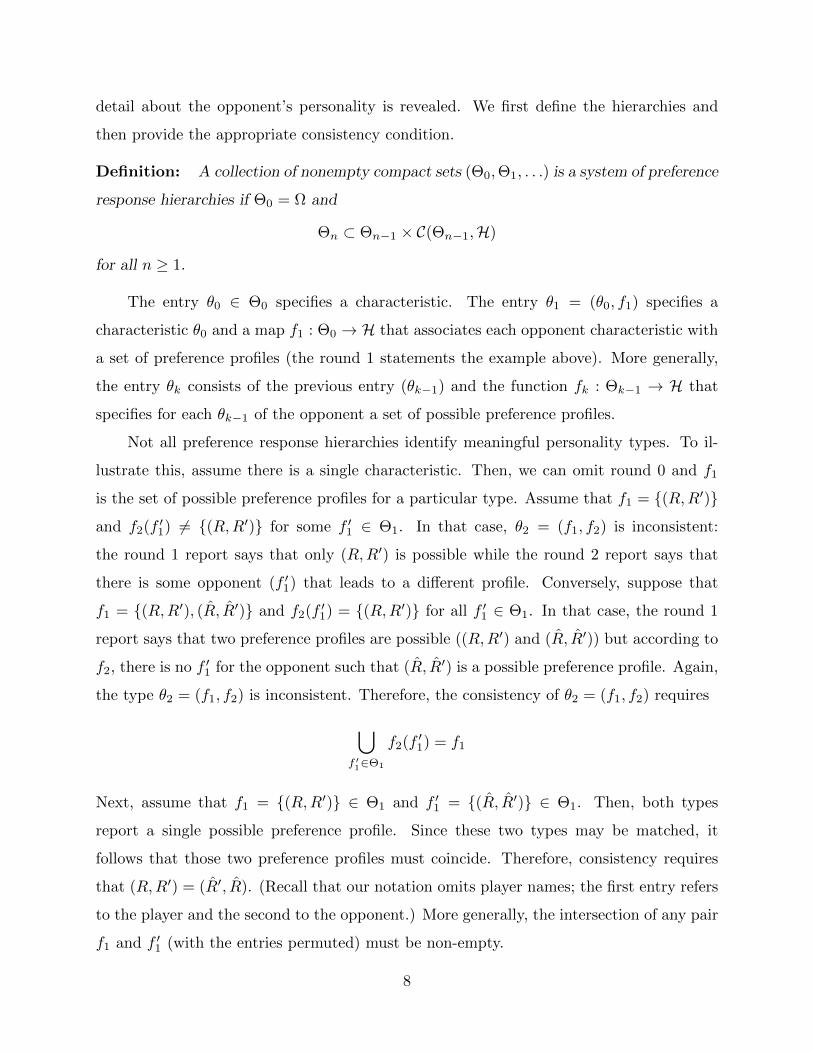
detail about the opponent’s personality is revealed. We first define the hierarchies and

then provide the appropriate consistency condition.

Definition: A collection of nonempty compact sets (Θ0,Θ1, . . .) is a system of preference

response hierarchies if Θ0 = Ω and

Θn ⊂ Θn−1 × C(Θn−1,H)

for all n ≥ 1.

The entry θ0 ∈ Θ0 specifies a characteristic. The entry θ1 = (θ0, f1) specifies a

characteristic θ0 and a map f1 : Θ0 → H that associates each opponent characteristic with

a set of preference profiles (the round 1 statements the example above). More generally,

the entry θk consists of the previous entry (θk−1) and the function fk : Θk−1 → H that

specifies for each θk−1 of the opponent a set of possible preference profiles.

Not all preference response hierarchies identify meaningful personality types. To il-

lustrate this, assume there is a single characteristic. Then, we can omit round 0 and f1

is the set of possible preference profiles for a particular type. Assume that f1 = (R,R′)and f2(f

′1) 6= (R,R′) for some f ′

1 ∈ Θ1. In that case, θ2 = (f1, f2) is inconsistent:

the round 1 report says that only (R,R′) is possible while the round 2 report says that

there is some opponent (f ′1) that leads to a different profile. Conversely, suppose that

f1 = (R,R′), (R, R′) and f2(f′1) = (R,R′) for all f ′

1 ∈ Θ1. In that case, the round 1

report says that two preference profiles are possible ((R,R′) and (R, R′)) but according to

f2, there is no f ′1 for the opponent such that (R, R′) is a possible preference profile. Again,

the type θ2 = (f1, f2) is inconsistent. Therefore, the consistency of θ2 = (f1, f2) requires

⋃

f ′1∈Θ1

f2(f′1) = f1

Next, assume that f1 = (R,R′) ∈ Θ1 and f ′1 = (R, R′) ∈ Θ1. Then, both types

report a single possible preference profile. Since these two types may be matched, it

follows that those two preference profiles must coincide. Therefore, consistency requires

that (R,R′) = (R′, R). (Recall that our notation omits player names; the first entry refers

to the player and the second to the opponent.) More generally, the intersection of any pair

f1 and f ′1 (with the entries permuted) must be non-empty.

8

The next definition below specifies the same two consistency requirements for all levels

of the hierarchy.

Definition: The system of preference response hierarchies (Θ0,Θ1, . . .) is consistent if:

(i) For all n ≥ 1, for all (θn−1, fn, fn+1) ∈ Θn+1, and for all θn−1 ∈ Θn−1

fn(θn−1) =⋃

f ′n | (θn−1,f ′

n)∈Θnfn+1(θn−1, f

′n)

(ii) For all (θn−1, fn), (θ′n−1, f

′n) ∈ Θn, there is (R,R′) ∈ R×R such that

(R,R′) ∈ fn(θ′n−1) and (R′, R) ∈ f ′

n(θn−1)

Given a consistent system of preference response hierarchies (Θ0,Θ1, . . .), we define a

type as a sequence (f0, f1, . . .) with the property that (f0, . . . , fn) ∈ Θn. To qualify as a

component of the canonical type space, Θ must satisfy an additional property. Every type

must generate a unique preference when confronted with any other type in the component

Θ. This means that for every pair of types (f0, f1, . . .), (f′0, f

′1, . . .) it must be the case that

fn(f′0, . . . , f

′n−1) converges to a singleton as n → ∞. Let θ(n) = (f0, f1, . . . , fn) denote the

n−truncation of the sequence θ = (f0, f1, . . .).

Definition: Let (Θ0,Θ1, . . .) be a consistent sequence of preference response hierarchies.

Let Θ := θ ∈ Θ0 ×∏∞

n=1 C(Θn−1,H) | θ(n) ∈ Θn. Then Θ is a component of behavioral

types if Θ is compact and if for all θ, θ′ ∈ Θ with θ = (f0, f1, . . .)

⋂n≥0 fn+1(θ

′(n)) is a singleton

The canonical type space is the union of all the components of behavioral types. Let

I denote the set of all components of interdependent types. The set

F =⋃

Θ∈IΘ

is the canonical behavioral type space or simply the canonical type space. Note that each

element θ ∈ F belongs to a unique component Θ ∈ I. Hence, I is a partition of F .

9

For any Θ ∈ I, let Ψ : Θ×Θ → R×R denote the function that specifies a preference

profile when the player is type θ and the opponent is type θ′. Hence,

Ψ(θ, θ′) :=⋂

n≥0

fn+1(θ′(n)) for (f0, f1, . . .) = θ

The function Ψ(θ, ·) is the personality of type θ. It describes how the player responds to

different opponent personalities. Requirement (ii) in the definition of consistency ensures

that the function ψ satisfies the following symmetry condition.

Ψ(θ, θ′) = (R,R′) implies Ψ(θ′, θ) = (R′, R) (S)

If Ψ satisfies (S), we say that Ψ is symmetric. We define φ : Θ → Ω × C(Θ,S) as the

function that specifies, for every type θ ∈ Θ, the characteristic of θ and the mapping θ

uses to assign preferences profile to opponent types. Hence,

φ(θ) := (f0,Ψ(θ, ·))

Theorem 1: The function Ψ is continuous and symmetric and φ is a homeomorphism

from Θ to φ(Θ).

It follows from Theorem 1 that any component Θ ∈ I is an (IPM): for a symmetric Ψ,

there is a ψ : Θ×Θ → R such that Ψ(θ, θ′) = (ψ(θ, θ′), ψ(θ′, θ)). Then, since Θ is compact

(by definition) and ψ is continuous (by Theorem 1), it follows that every component of the

canonical type space is an IPM. We record this observation as a corollary.

Corollary: If Θ ∈ I, then (Θ, ψ, ω) is an IPM.

10

3. Valid Models

Suppose the environment has a single characteristic and two possible preferences, a

and b. Consider the following IPM:

1 21 (a, a) (b, b)2 (b, b) (a, a)

Table 3

This IPM is not an element of the canonical type space. To see why not, note that all

types have the same characteristic, there is nothing to report in round 0. The round 1 set

of possible preference profiles is (a, a), (b, b) for both players. Since round 1 statements

are identical for both types, all higher round statements must be identical as well. Hence,

for all n the function fn is constant (with value (a, a), (b, b)). The two types in this IPM

have identical preference response hierarchies.

The IPM in table 3 illustrates a case in which the IPM introduces a distinction between

types 1 and 2 that has no counterpart in terms of the model’s primitives. Every preference

statement that holds for type 1 is also true for type 2. Therefore, we cannot express the

personalities of those two types as preference statements.

We can interpret the IPM in table 3 as an incomplete model. For example, it might

be that the model omits a type.

1 2 31 (a, a) (b, b) (b, a)2 (b, b) (a, a) (a, a)3 (a, b) (a, a) (a, a)

Table 4

In the IPM in table 4, type 3 always prefers a irrespective of the opponent’s type. Type 2

accommodates this preference while type 2 does not. Hence, types 1 and 2 have different

personalities, and can be distinguished through their response to type 3. The IPM depicted

in table 3 could be interpreted as table 4 with an omitted type.

Alternatively, it might be that the model has omitted a characteristic: if types 1 and

2 have different characteristics (type 1 is wealthy, type 2 is poor) then the IPM in table 3

11

is a component of the canonical type space: both types have preference a if the opponent’s

has the same wealth and preference b otherwise.

The two interpretations have obviously very different implications for applications. If

players’ behavior depends on the opponent’s wealth (an omitted characteristic) then the

observability of wealth is a key determinant of outcomes. If players’ behavior depends on

their response to some third personality type (type 3) then observability of wealth should

have no effect and instead the observability of past play will affect outcomes. Since the

IPM is not a component of the canonical type space, we cannot express personalities in

terms of the underlying primitives of the model. As a result, we cannot determine how

information about the underlying primitives affects behavior.

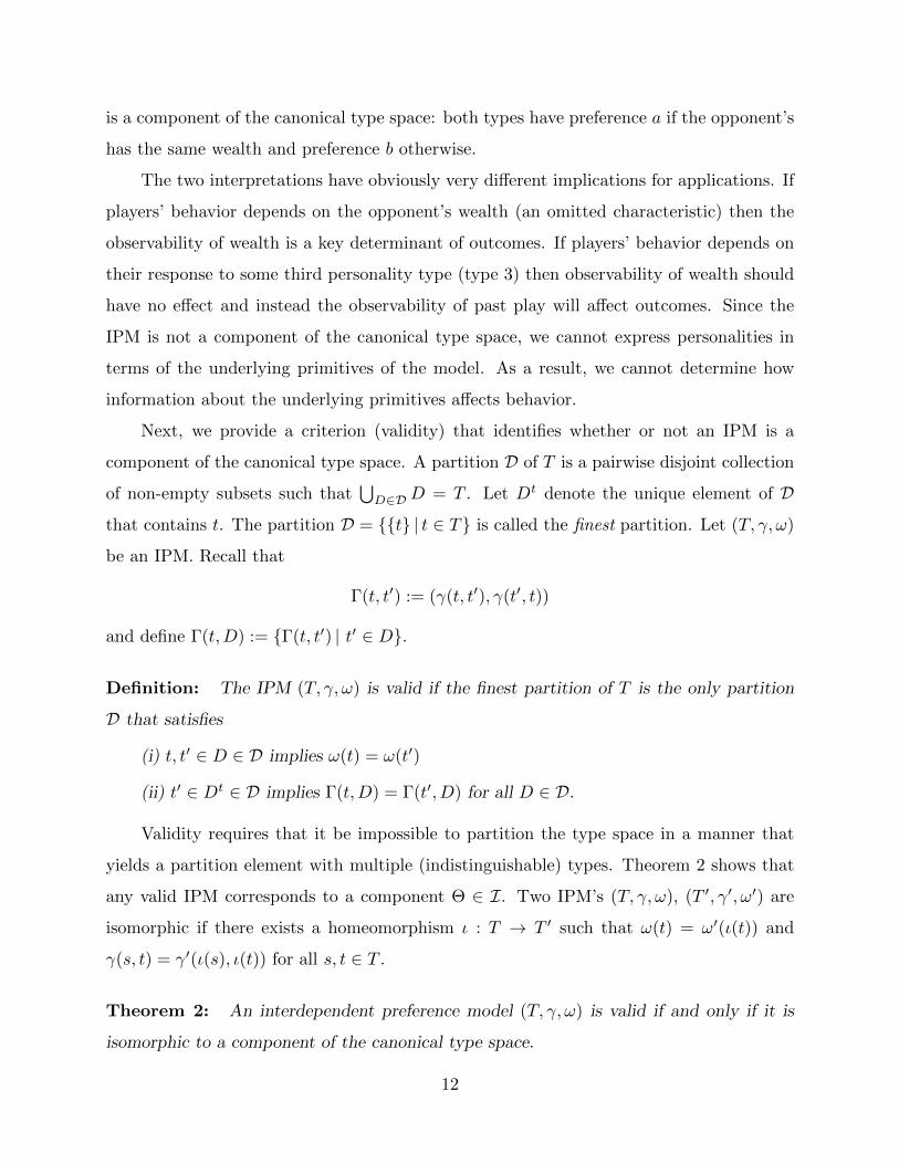
Next, we provide a criterion (validity) that identifies whether or not an IPM is a

component of the canonical type space. A partition D of T is a pairwise disjoint collection

of non-empty subsets such that⋃

D∈D D = T . Let Dt denote the unique element of Dthat contains t. The partition D = t | t ∈ T is called the finest partition. Let (T, γ, ω)

be an IPM. Recall that

Γ(t, t′) := (γ(t, t′), γ(t′, t))

and define Γ(t,D) := Γ(t, t′) | t′ ∈ D.

Definition: The IPM (T, γ, ω) is valid if the finest partition of T is the only partition

D that satisfies

(i) t, t′ ∈ D ∈ D implies ω(t) = ω(t′)

(ii) t′ ∈ Dt ∈ D implies Γ(t,D) = Γ(t′, D) for all D ∈ D.

Validity requires that it be impossible to partition the type space in a manner that

yields a partition element with multiple (indistinguishable) types. Theorem 2 shows that

any valid IPM corresponds to a component Θ ∈ I. Two IPM’s (T, γ, ω), (T ′, γ′, ω′) are

isomorphic if there exists a homeomorphism ι : T → T ′ such that ω(t) = ω′(ι(t)) and

γ(s, t) = γ′(ι(s), ι(t)) for all s, t ∈ T .

Theorem 2: An interdependent preference model (T, γ, ω) is valid if and only if it is

isomorphic to a component of the canonical type space.

12

We have interpreted the invalid IPM above as an incomplete model, either missing

types or missing characteristics. Note that any finite invalid IPM can be “validated” by

adding new types or new characteristics. Any model is obviously valid if each type has

a distinct characteristic. For the missing types interpretation, it is easy to show that

any finite, invalid IPM can be embedded in a valid IPM with a larger type space. More

precisely, assume that R contains at least 2 preferences and consider a finite IPM (T, γ, ω).

Then, there exists a valid IPM (T , γ, ω) such that T ⊂ T , γ(t) = γ(t) for all t ∈ T and

ω(t) = ω(t) for all t ∈ T .

4. Validity and Communicability

We have interpreted preference response hierarchies as players’ conditional preference

statements that gradually reveal their type. Those hierarchies impose a particular protocol

of how these statements unfold. In this section, we show that no other protocol can do

better. More formally, we introduce a general framework for communication and show

that agents can reveal their types through communication if and only if the IPM is valid.

Hence, types are communicable if and only if the IPM is a component of the canonical

type space.

For simplicity, we assume that there is single characteristic4 and a finite number of

behavioral types. To formulate a model of communication, we need to translate the IPM

into an epistemic model. An epistemic model is a finite set of states S, a map ν : S → R×Rthat associates a preference profile with each state and a pair of partitions T1 and T2 of S

that represent the players’ knowledge. Elements of Ti are player i’s epistemic types.

Let (T, γ) be an IPM with a single characteristic and a finite set of types. In the

equivalent epistemic model, each player knows his own type and knows nothing about

his opponent’s type; that is, any type in T possible. Formally, the epistemic model E =

S, T1, T2, ν is equivalent to the IPM (T, γ) if there is a bijection ζi : T → Ti such that

Γ(t, t′) = ν(ζ1(t) ∩ ζ2(t′)) for all t, t′ ∈ T . The bijection ζi maps behavioral types (of

M) into epistemic types (of E) while preserving the resulting preference profile. We refer

to E as an IPM in epistemic form (IPM-EF).

4 Extending the analysis below to IPMs with multiple characteristics is straightforward. We assume asingle characteristic to keep the notation simple.

13

A collection of subsets K of a set S is an algebra (or equivalently, a language) if it

contains S and is closed under unions and complements. For any two algebras K,L, letK ∨ L denote the smallest (in terms of set inclusion) algebra that contains both and let

K ∧ L be the largest that is contained in both.

We call each A ∈ L is a word. The primitives of an interactive preference model are

preference statements. Hence, the relevant language is the the language of preferences.5 A

subset A of S is a word in the language of preferences if A = s ∈ S | ν(s) ∈ V for some

set of preference profiles V ∈ H.

Definition: The language of preferences is Lp = A ⊂ S |A = ν−1(V ), V ∈ H.

To illustrate these definitions, we apply them to Example 1 from the previous section.

Example 1′: (epistemic form) Let T = 1, . . . , k and define γ as in Example 1 above:

γ(i, j) =

G if i+ j > kS if i+ j ≤ k

Then, define S, T1, T2, ν equivalent to (T, γ) as follows: let S = (i, j) | i ∈ T, j ∈ Tand ν(i, j) = (γ(i, j), γ(j, i)) for all (i, j) ∈ S. The information partitions are T1 =

(i, 1), . . . , (i, k) | i ∈ T and T2 = (1, i), . . . , (k, i) | i ∈ T.There are two possible preference profiles, G,G and S, S. Therefore, the language

of preferences has three non-empty words: A = (i, j) | i+ j > k, B = (i, j) | i+ j ≤ kand S = A ∪ B. The word A corresponds to (G,G), B corresponds to (S, S) and

S = A ∪B corresponds to (S, S), (G,G).

A person with knowledge Ti can use the word A ∈ L to make a statement about

whether or not he knows A. Let

Ti ∗A :=⋃

B∈Ti,B⊂A

B

Then, i can use the word A to communicate the words Ti ∗A, Ti ∗ (S\A) to j. These are

words derived from A and S\A that i understands; that is, at every s ∈ S, i knows whether

5 The formalism developed here can be used to define communicability with respect to any givenlanguage.

14

or not Ti ∗ A and Ti ∗ (S\A)) applies (i.e., is true); he knows whether or not he knows

A and he knows whether or not he knows S\A. Then, using standard logical operations

he can also communicate other words such as [S\(Ti ∗A)] ∩ [S\(Ti ∗ (S\A))]; i.e., that he

knows neither A nor S\A. We let

Ti ∗ L

denote the language that can be communicated in this way. That is, Ti ∗ L is the smallest

algebra that contains Ti ∗A for every A ∈ L.6

Let Λ be the collection of all algebras and let Λp := L ∈ Λ | Lp ⊂ L.7 Define the

function F : Λp → Λp as follows:

F (L) = L ∨ [T1 ∗ L] ∨ [T2 ∗ L]

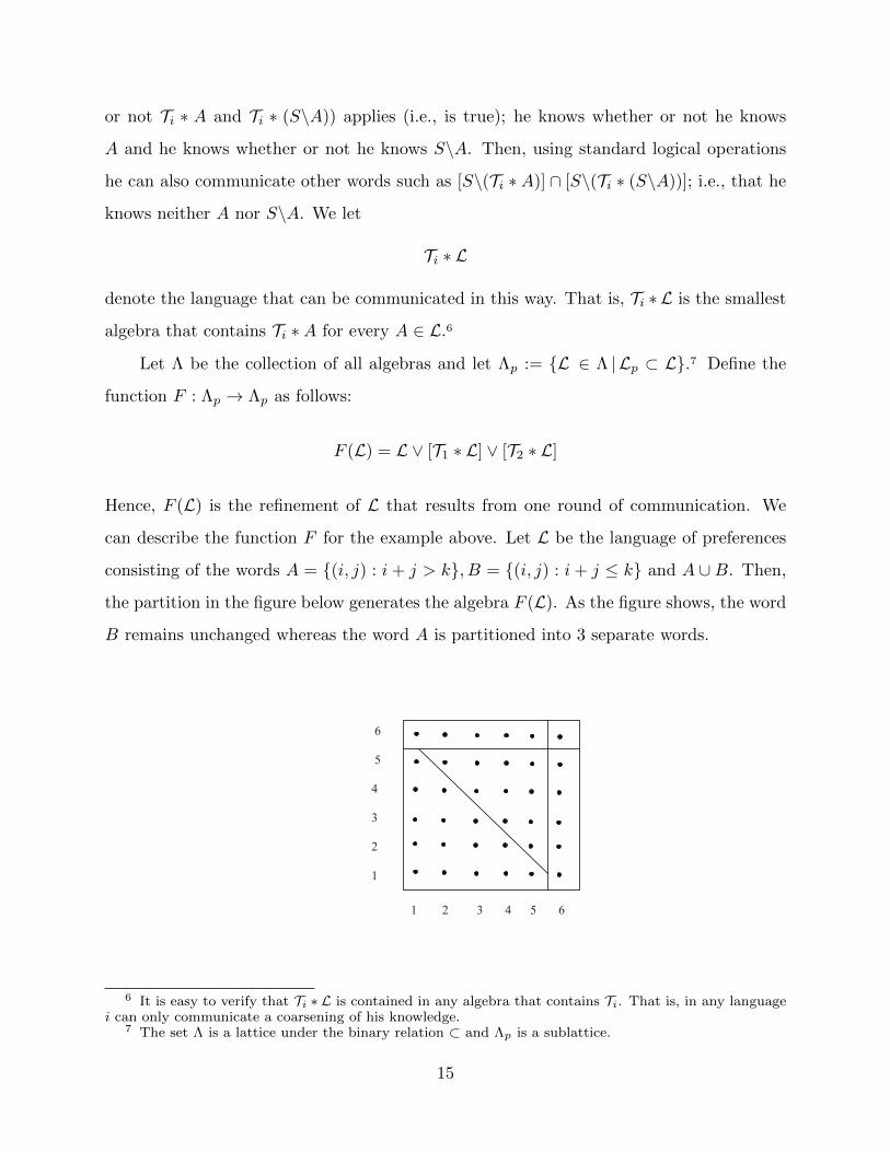
Hence, F (L) is the refinement of L that results from one round of communication. We

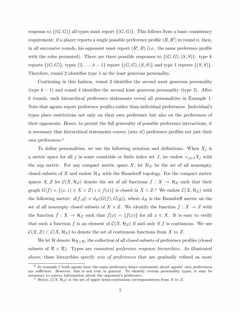
can describe the function F for the example above. Let L be the language of preferences

consisting of the words A = (i, j) : i+ j > k, B = (i, j) : i+ j ≤ k and A ∪ B. Then,

the partition in the figure below generates the algebra F (L). As the figure shows, the wordB remains unchanged whereas the word A is partitioned into 3 separate words.

1 2 3 4 5 6

6

5

4

3

2

1

6 It is easy to verify that Ti ∗ L is contained in any algebra that contains Ti. That is, in any languagei can only communicate a coarsening of his knowledge.

7 The set Λ is a lattice under the binary relation ⊂ and Λp is a sublattice.

15

Let L1 = Lp and inductively define Ln+1 = F (Ln). Players can continue communicat-

ing until they reach a fixed point of F . Since S is finite, there is n such that F (Ln) = Ln.

Let L∗ denote this fixed point. Through this process, players can communicate the algebra

Cp := [T1 ∗ L∗] ∨ [T2 ∗ L∗]

Then, a collection of subsets M of S is communicable if only if M ⊂ Cp.In the sequence L1,L2, . . . players communicate all information in each round. Con-

sider any other sequence L1, L2, . . . starting at the same initial point L1 = Lp such that in

each round agents exchange some (but not necessarily all) of their information until they

reach a situation in which they have nothing new to convey. This process will refine the

language until a fixed point L of F is reached. We claim that L = L∗. To see this, observe

that F is a monotone function, that is,

L′ ⊂ L′′ implies F (L′) ⊂ F (L′′)

Applied to the fixed point L, the equation above implies F (L) ⊂ L if L ⊂ L. Since

L1 ⊂ L, we conclude that Ln ⊂ L for all n and therefore L∗ ⊂ L. That L ⊂ L∗ follows

from the fact that Ln ⊂ Ln for all n (by construction). Hence, L∗ = L and L∗ is the

outcome any communication protocol. A particular collection of subsets is communicable

in Lp if this collection is contained in Cp. We wish to characterize when players’ types are

communicable.

Definition: An IPM (S, T1, T2, ν) in epistemic form is communicable in language Lp if

Ti ⊂ Cp for i = 1, 2.

An IPM is communicable if players can express their types in the language of pref-

erences. Theorem 3 below shows that validity identifies exactly those models that can be

communicated.

Theorem 3: A finite IPM in epistemic form is communicable in the language of prefer-

ences if and only if it is equivalent to a valid IPM.

We interpret communicability as a test that a well-defined, self-contained model of

interdependent preferences types must satisfy: responding to the opponent’s personality

16

requires understanding his personality and each player’s understanding is the sum of what

he knows at the outset (i.e., his type) and what he can learn through communication

with the other player.8 A model that violates this communicability test can, at best, be

interpreted as an incomplete model: players respond to personality types that are well

defined in a larger context (in a richer model) but ill-defined in the IPM at hand.

5. Reciprocity

A reciprocating personality9 is one that is kinder to nicer opponents. Hence, in our

formal definition of reciprocity, we assume an exogenous “kindness” ranking on preferences.

The literature often assumes that individuals have exogenously specified selfish utilities

and identifies altruism (or generosity or kindness) with the relative weight a person puts

on other’s selfish utility. For example, let (x, y) ∈ A = [0, 100] × [0, 100] be the vector

consumptions and assume that selfish utilities are linear. Then, let Ur such that

Ur(x, y) = x+ ry

be the utility function representing preference with parameter r ∈ [−1, 1]. A natural

kindness order on these preferences is the “≥” ranking of their parameters. That is, the

preference (with parameter) r is kinder than the preference r′ if and only if r ≥ r′.

More generally, we assume that there is a continuous one-to-one function τ : R → IR

and interpret τ(R) ≥ τ(R′) to mean R is kinder than R′. We say that M is an ordered IPM

when such τ exists. When the IPM is ordered, it is convenient to identify each preference

R with τ(R) and suppress preferences. Then, we let δ = τ γ and refer to (T, δ) as an

ordered IPM.

Definition: In an ordered IPM, type t is nicer than type t′ if δ(t, t′′) ≥ δ(t′, t′′) for all

t′′; type t reciprocates if δ(t, t′) ≥ δ(t, t′′) whenever t′ is nicer than t′′. An ordered IPM is a

reciprocity model if it is valid, the niceness relation is complete and every type reciprocates.

8 Since we wish to identify what can be understood in principle, we are ignoring incentives. In practice,an agent may learn less than Cp since his opponent may strategically withhold information.

9 For simplicity, we assume throughout this section that all types have the same characteristic andhence use type and personality interchangeably.

17

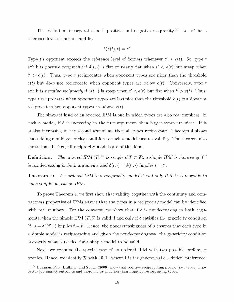
This definition incorporates both positive and negative reciprocity.10 Let r∗ be a

reference level of fairness and let

δ(e(t), t) = r∗

Type t’s opponent exceeds the reference level of fairness whenever t′ ≥ e(t). So, type t

exhibits positive reciprocity if δ(t, ·) is flat or nearly flat when t′ < e(t) but steep when

t′ > e(t). Thus, type t reciprocates when opponent types are nicer than the threshold

e(t) but does not reciprocate when opponent types are below e(t). Conversely, type t

exhibits negative reciprocity if δ(t, ·) is steep when t′ < e(t) but flat when t′ > e(t). Thus,

type t reciprocates when opponent types are less nice than the threshold e(t) but does not

reciprocate when opponent types are above e(t).

The simplest kind of an ordered IPM is one in which types are also real numbers. In

such a model, if δ is increasing in the first argument, then bigger types are nicer. If it

is also increasing in the second argument, then all types reciprocate. Theorem 4 shows

that adding a mild genericity condition to such a model ensures validity. The theorem also

shows that, in fact, all reciprocity models are of this kind.

Definition: The ordered IPM (T, δ) is simple if T ⊂ IR; a simple IPM is increasing if δ

is nondecreasing in both arguments and δ(t, ·) = δ(t′, ·) implies t = t′.

Theorem 4: An ordered IPM is a reciprocity model if and only if it is isomorphic to

some simple increasing IPM.

To prove Theorem 4, we first show that validity together with the continuity and com-

pactness properties of IPMs ensure that the types in a reciprocity model can be identified

with real numbers. For the converse, we show that if δ is nondecreasing in both argu-

ments, then the simple IPM (T, δ) is valid if and only if δ satisfies the genericity condition

(t, ·) = δ∗(t′, ·) implies t = t′. Hence, the nondecreasingness of δ ensures that each type in

a simple model is reciprocating and given the nondecreasingness, the genericity condition

is exactly what is needed for a simple model to be valid.

Next, we examine the special case of an ordered IPM with two possible preference

profiles. Hence, we identify R with 0, 1 where 1 is the generous (i.e., kinder) preference,

10 Dohmen, Falk, Huffman and Sunde (2009) show that positive reciprocating people (i.e., types) enjoybetter job market outcomes and more life satisfaction than negative reciprocating types.

18

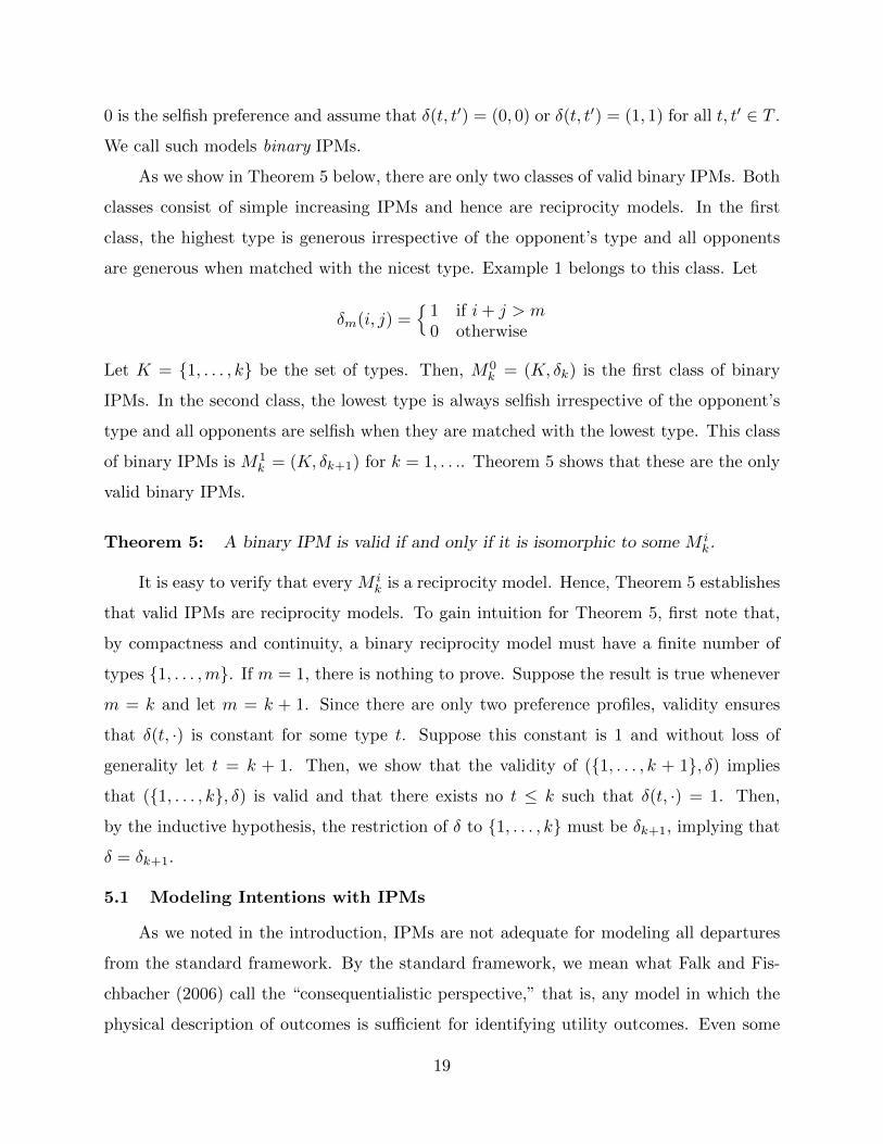
0 is the selfish preference and assume that δ(t, t′) = (0, 0) or δ(t, t′) = (1, 1) for all t, t′ ∈ T .

We call such models binary IPMs.

As we show in Theorem 5 below, there are only two classes of valid binary IPMs. Both

classes consist of simple increasing IPMs and hence are reciprocity models. In the first

class, the highest type is generous irrespective of the opponent’s type and all opponents

are generous when matched with the nicest type. Example 1 belongs to this class. Let

δm(i, j) =1 if i+ j > m0 otherwise

Let K = 1, . . . , k be the set of types. Then, M0k = (K, δk) is the first class of binary

IPMs. In the second class, the lowest type is always selfish irrespective of the opponent’s

type and all opponents are selfish when they are matched with the lowest type. This class

of binary IPMs is M1k = (K, δk+1) for k = 1, . . .. Theorem 5 shows that these are the only

valid binary IPMs.

Theorem 5: A binary IPM is valid if and only if it is isomorphic to some M ik.

It is easy to verify that every M ik is a reciprocity model. Hence, Theorem 5 establishes

that valid IPMs are reciprocity models. To gain intuition for Theorem 5, first note that,

by compactness and continuity, a binary reciprocity model must have a finite number of

types 1, . . . ,m. If m = 1, there is nothing to prove. Suppose the result is true whenever

m = k and let m = k + 1. Since there are only two preference profiles, validity ensures

that δ(t, ·) is constant for some type t. Suppose this constant is 1 and without loss of

generality let t = k + 1. Then, we show that the validity of (1, . . . , k + 1, δ) implies

that (1, . . . , k, δ) is valid and that there exists no t ≤ k such that δ(t, ·) = 1. Then,

by the inductive hypothesis, the restriction of δ to 1, . . . , k must be δk+1, implying that

δ = δk+1.

5.1 Modeling Intentions with IPMs

As we noted in the introduction, IPMs are not adequate for modeling all departures

from the standard framework. By the standard framework, we mean what Falk and Fis-

chbacher (2006) call the “consequentialistic perspective,” that is, any model in which the

physical description of outcomes is sufficient for identifying utility outcomes. Even some

19

forms of reciprocity may fall outside of the reach of IPMs. For example, a player may

care only about whether or not another player acted generously and not about the other

player’s (persistent) personality.11

However, when modeling intentions, identifying persistent attributes as the carriers of

utility has some advantages. We considered one of those advantages in the introduction:

the implied separation of preferences from institutions facilitates the analysis of economic

design problems. Here, we will discuss a second advantage: it enables reciprocity models

to differentiate between acting generously out of self-interest and genuine kindness.

Berg, Dickhuat and McCabe (1995) provide experimental evidence indicating that

(i) subjects often act generously towards others and trust them to reciprocate and (ii)

this trust/generocity is often rewarded. Berg, Dickhuat and McCabe consider factors that

might facilitate such trust and reciprocity. Our goal in this subsection is to suggest a

novel experiment that would enable the experimenter to determine if this trust/generocity

reflects genuine concern for the opponent or if it is strategic and motivated by the expec-

tation of reciprocity. Then, we show how our theory might be useful for organizing the

results of such an experiment.

Consider the following game: player 1 is either generous/trusts (g) player 2 or he does

not (s). Afterwards, nature chooses either 0 or 1. If nature chooses 0, the game ends. The

outcome (g, 0) yields (70, 30); that is, 70 dollars for player 1 and 30 dollars for player 2

while (s, 0) yields (80, 0). If nature chooses 1, then player 2 chooses an action; she either

accepts player 1’s decision (a) or declines it (d). The outcomes (g, 0) and (g, 1, a) yield

the monetary payoffs (70, 30) while (s, 0) and (s, 1, a) yield the monetary payoffs (80, 0).

If player 2 chooses d, she gets 40 dollars and player 1 gets 0 dollars. That is, (g, 1, d) and

(s, 1, d) both yield the monetary payoffs (0, 40). Let α ∈ (0, 1) be the probability that

nature chooses 1.

Consider how changing α might affect behavior. First, let α be close to 1. Then, if

player 1 chooses s and nature chooses 1, player 2 is likely to choose d: by choosing s, player

1 has shown no generocity/trust and therefore player 2 is likely to be ungenerous as well.

Knowing this, player 1 believes he is likely to get 0 if he chooses s. Hence, when α is high,

11 Falk and Fischbacher’s (2006) definition of reciprocity reflects this view.

20

player 1 will be inclined to choose g even if he puts no weight 2’s well-being. Thus, player

1’s generocity/trust in this case may be strategic.

In contrast, when α is close to zero, the action g reveals a genuinely generous player

1; had he chosen s, he would have (almost) guaranteed himself 80 and he is giving this up

for player 2’s benefit. Therefore, conditional on the node (g, 1) being reached, we would

expect player 2 to be more inclined to honor player 1’s trust when α is low than when it

is high.

Thus, when α is close to 0, g is proof of player 1’s good intentions (i.e., that he is

type 2) and is fully rewarded. When α is close to 1, g can mean that player 1 has good

intentions or that he would like player 2 to think he has good intentions. The possibility

that player 1’s generosity is not genuine should make player 2’s less reciprocating.

To see how a reciprocity model can match the intuition outlined above, we will model

preferences with the binary IPM M02 defined in the previous section. To be concrete, let

r ∈ 0, 1 be the preference that Ur below represents:

Ur(x, y) = x+ ry

Then, consider the IPM (1, 2, δ), where

δ(t, t′) = 1 if and only if t+ t′ > 2.

Assume that both players are drawn from the same population with 10% type 2’s.

For α sufficiently small, the game above has a unique equilibrium: player 1 chooses g if

and only if he is type 2 and player 2 always accepts g and accepts s if and only if she is

type 2. For α close to 1, the game again has a unique equilibrium: player 1 chooses g for

sure if he is type 2 and randomizes between g and s if he is type 1. Player 2 accepts g for

sure if she is type 2 and randomizes between a and d if she is type 2.

These two equilibria match the intuition above exactly: if α is close to 0, choosing g is

unambiguously generous and such generosity is rewarded. If α is close to 1, both generosity

and self-interest are possible motives for choosing g and therefore player 2’s response is

more qualified; sometimes she reciprocates and sometimes she doesn’t.

21

With interdependent preferences, different game forms create different incentives to

reveal (or conceal) intentions. Understanding the behavioral consequences of a particu-

lar institution or environmental factor, then, amounts to understanding the incentives it

creates for signalling intentions.

6. Related Literature on Belief (or Possibility) Hierarchies

That each types can be identified with a unique hierarchy of preference statements

is a central property of our model. The same objective – relating differences in types to

differences in payoff relevant primitives – can also be pursued when types are exogenous pa-

rameters.12 Bergemann and Morris (2007), (2009) and Bergemann, Morris and Takahashi

(2010) establish that this question plays a central role in implementation theory. Berge-

mann and Morris (2007) permits asymmetric information (i.e., players form conjectures

over their opponents’ preference types) and they prove two results in which conditions

similar to validity play a role.

To facilitate the comparison, we consider finite, symmetric two-person IPMs with

a single characteristic.13 Each pair of types yields a pair of von Neumann-Morgenstern

utilities on Z, the set of all lotteries over outcomes. Let (T, γ) be an IPM satisfying

these conditions and assume that the two agents are playing an arbitrary two-person game

G = A1, A2, g, where g : A1 × A2 → Z. Hence, Ai is player i’s pure strategy set and

g is the outcome function that relates pure strategy profiles to lotteries over outcomes.

Bergemann and Morris make a mild genericity assumption: given any belief over opponent

types and actions, no type is ever indifferent over all of his own actions.

Bergemann and Morris define rationalizable actions as follows: each round, players

are allowed any conjecture over opponent types and allowed actions for those types. Then,

actions that are never best responses for a type against all such conjectures are eliminated

and become no longer unavailable for that type. Actions that are never eliminated are

rationalizable. Bergemann and Morris (2007) call two types strategically equivalent if

12 For example, Ely and Peski (2006) point out that in standard models of incomplete information,two different types may have exactly the same hierarchy of beliefs. See also Dekel, Fudenberg and Morris(2006a), (2006b) for related work. In an earlier version of this paper (Gul and Pesendorfer (2005)), weshow that an IPM is valid if and only if each type is uniquely identified through its possibility hierarchy.The latter concept is due to Mariotti, Meier and Piccione (2005).

13 Bergemann and Morris (2007) allow for arbitrary finite n−person IPMs.

22

they have the same set of rationalizable actions in every game. To relate their Proposition

5 to our analysis of communicability, we present the following stronger notion of validity:

Definition: The IPM (T, γ, ω) is strongly valid if the finest partition of T is the only

partition D that satisfies

(i) t, t′ ∈ D ∈ D implies ω(t) = ω(t′)

(ii) t′ ∈ Dt ∈ D implies γ(t,D) = γ(t′, D) for all D ∈ D.

The difference between validity and strong validity is that γ replaces Γ in the latter.

Hence, strong validity would be the appropriate concept for Theorem 1 (or Theorem 3) if

each player were restricted to making statements about his own preferences. We can now

state Proposition 5 of Bergemann and Morris (2007) as follows:

Proposition: If (γ, T ) satisfies the genericity condition above and fails strong validity,

then there are at least two equivalent types in T .

We can relate the result above to Theorem 3 as follows: if two types cannot distinguish

themselves through any (truthful) preference statement, then they certainly cannot distin-

guish themselves through their strategic behavior. Of course, a type may have knowledge

about preferences that is not strategically relevant, for example, he may know facts about

his opponent’s preferences that the opponent does not know. Hence, validity is not enough

to rule out strategically equivalent types but the failure of validity ensures that there are

strategically equivalent types.

While formally related, Theorem 3 and the proposition above have different objectives

and interpretations. Theorem 3 asks if a particular IPM can be interpreted as a legiti-

mate, non-circular description of individuals’ attitudes toward each other. It identifies

the following test: for an IPM to be valid, given any type profile, there should be some

sequence of statements (about preferences) that would enable both players to figure out

their opponents’ types. Hence, we interpret validity as a constraint on the modeler; IPMs

that fail validity will have types that cannot be distinguished except through the arbitrary

notational devices of the modeler.

In contrast, Bergemann and Morris have in mind situations in which types have clear

meaning; that is, they view types as privately observed characteristics. For example,

23

suppose there are two kinds of two-way radios (A and B). Suppose also that the two

players derive utility only if both have the same kind of radio and invest a dollar to

activate their radios. Hence, there are two outcomes, activate (1) and don’t activate (0).

When a type A confronts a type A or a type B confronts a type B, both prefer 1 to 0.

Otherwise, both prefer 0 to 1. In this example, if we interpret A and B as types rather

than characteristics validity fails. The proposition above implies that both types will have

exactly the same set of rationalizable strategies in every game. This does not mean that

the model is in any sense ill-defined; being type A or B has a clear meaning in this model.

However, as Bergemann and Morris show, no social choice rule that treats types A and B

differently can be robustly implemented.14

Aumann (1976) shows that in a finite asymmetric information model with a common

prior if the posteriors are common knowledge, then they must be identical. Geanakoplos

and Polemarchakis (1982) investigate how posteriors might become common knowledge.

They show that if two agents exchange information by sequentially revealing their current

probability assessments (of a particular event), then, eventually, these assessments will be-

come common knowledge (and hence, common if the priors are common as well) whenever

a mild genericity condition is satisfied. The subsequent literature on communication and

consensus extends this result in the following ways: the function being communicated is

not just priors but an arbitrary mapping from the set of all events,15 there are more than

two communicating agents and explicit, general protocols determining who speaks when.16

In these papers, the medium of communication; that is, the language is an arbitrary

function g : 2S\∅ → Y such that

g(E) = g(E′), E ∩ E′ = ∅ implies g(E ∪ E′) = g(E) (C)

Agents take turns announcing g(E) to some subset of other agents, where E ⊂ S is the

smallest event that the agent knows to be true given all that he has heard before. These

14 Bergemann and Morris’ main theorem shows that a condition stronger than strong validity is neces-sary and sufficient to ensure that for any distinct t, t′, there exist some game G in which set of rationalizablestrategies of t and t′ are disjoint. They show that the latter property plays a key role in robust implemen-tation with simultaneous mechanisms.

15 See for example, Cave (1983) and Bacharach (1985).16 See Parikh and Krasucki (1990).

24

papers identify conditions on g and the protocol that ensure that eventually all agents

have the same knowledge about the value of g. Despite the absence of priors in our model,

some comparisons between Theorem 3 and the results in this literature are possible. Our

language of preferences yields the following function g:

g(E) = ν(s) | s ∈ E

Thus, an agent who knows the event E, knows that the true preference profile is in g(E).

This g satisfies the convexity condition (C) above. The standard consensus result of the

literature corresponds to the assertion that T1 ∗G(L) = T2 ∗G(L); that is, once communi-

cation stops the two agents have the same knowledge about preferences (i.e., the function

g). Note that our focus is on whether types can be communicated in the language of

preferences rather than whether communicating in the language of preferences eventually

leads to agreement about preferences.

Our notion of communication is more permissive than the Caves-Bacharach-Parikh

and Krasucki model of communication protocols. Our modeling has the effect of per-

mitting conditional statements such as “had you told me x, I would have said y.” A

communication protocol does not permit such statements. Hence, our version of com-

munication always leads to (weakly) more “knowledge sharing” than any communication

protocol. Furthermore, there are examples in which our model can convey knowledge that

cannot be conveyed through all possible protocols.

7. Appendix

Let Z be a compact metric space. For any sequence An ∈ HZ , let

limAn = z ∈ Z | z = lim zn for some sequence zn such that zn ∈ An for all nlimAn = z ∈ Z | z = lim znj for some sequence znj such that znj ∈ Anj for all j

Let X be a metric space and p : X → HZ . We say that p is Hausdorff continuous if it is a

continuous mapping from the metric space X to the metric space HZ . Note that if p is a

Hausdorff continuous mapping from X to HZ , then p ∈ C(X,HZ). However, the converse

is not true.

25

Lemma 1: Let X,Y, Y ′, Z be nonempty compact metric spaces, q ∈ C(X × Y, Z), p ∈C(Y ′,HY ), and r ∈ C(Y ′, Y ). Then, (i) An ∈ HZ converges to A (in the Hausdorff

topology) if and only if limAn = limAn = A. (ii) xn ∈ X converges to x implies q(xn, B)

converges to q(x,B) for all B ∈ HY . (iii) If q∗(x, y′) = q(x, p(y′)) for all x ∈ X, y′ ∈ Y ′

then q∗ ∈ C(X × Y ′,HZ). (iv) If r is onto, then r−1 ∈ C(Y,HY ′).

Proof: Part (i) is a standard result. See Brown and Pearcy (1995).

(ii) Suppose xn ∈ X converges to x. Let znj∈ q(xnj

, B) such that lim znj= z. Hence,

znj= q(xnj

, ynj) for some ynj

∈ B. Since B is compact, we can without loss of generality

assume ynj converges to some y ∈ B. Hence, the continuity of q ensures z = q(x, y)

and therefore z ∈ q(x,B) proving that limq(xn, B) ⊂ q(x,B). If z ∈ q(x,B), then there

exists y ∈ B such that z = q(x, y). Since q is continuous, we have z = lim q(xn, y).

Hence, q(x,B) ⊂ limq(xn, B). Since, limq(xn, B) ⊂ limq(xn, B) ⊂ q(x,B), we conclude

limq(xn, B) = q(xn, B) = limq(xn, B) as desired.

(iii) Suppose (xn, y′n) converges to (x, y) and zn ∈ q∗(xn, y

′n) converges to z. Pick

yn ∈ p(y′n) such that q(xn, yn) = zn. Since Y is compact, we can assume that yn converges

to some y. Since p ∈ C(Y ′,HY ), we conclude that y ∈ p(y′) and since q is continuous,

q(x, y) = z. Therefore, z ∈ q∗(x, y′), proving that q∗ ∈ C(X × Y,HZ).

(iv) The continuity and ontoness of r ensures that r−1 maps Y into hY ′ . Assume that

yn converges to y, y′n ∈ r−1(yn) and y′n converges to y′. Then, r(y′n) = yn for all n and by

continuity r(y′) = y. Therefore, y′ ∈ r−1(y) as desired.

Lemma 2: Let X and Z be compact metric spaces. Suppose pn ∈ C(X,HZ) and

pn(x) ⊂ pn+1(x) for all n ≥ 1, x ∈ X. Let p(x) :=⋂

n≥1 pn(x) and assume p(x) is a

singleton for all x ∈ X. Then, (i) p is continuous and (ii) pn converges to p.

Proof: Obviously,⋂

n≥1 G(pn) = G(p). Since pn ∈ C(X,HZ) and X,Z are compact, so is

G(pn). Therefore G(p) is compact (and therefore closed) as well. Since p is a function and

both X,Z are compact, the fact that p has a closed graph implies that p is continuous.

To prove (ii), it is enough to show that if Gn is a sequence of compact sets such that

Gn+1 ⊂ Gn then Gn converges (in the Hausdorff topology) to G :=⋂

n Gn. If not, since

G1 is compact, we could find ε > 0 and yn ∈ Gn converging to some y ∈ G1 such that

26

d(yn, G) > ε for all n. Hence, d(y,G) ≥ ε and therefore there exists k such that y /∈ Gk for

all n ≥ k. Choose ε′ > 0 such that miny′∈Gkd(y′, y) ≥ ε′ and k′ such that n ≥ k′ implies

d(yn, y) < ε′/2. Then, for n ≥ maxk, k′ we have d(yn, y) ≥ ε′ and d(yn, y) < ε′/2, a

contradiction.

We say that pn ∈ C(X,HZ) converges to p ∈ C(X,HZ) uniformly if for all ε > 0,

there exists N such that n ≥ N implies d(pn(x), p(x)) < ε. Let X be an arbitrary set

and Z be a compact metric space. Given any two functions p, q that map X into HZ , let

d∗(p, q) = supx∈X d(p(x), q(x)), where d is the Hausdorff metric on HZ .

Lemma 3: (i) If pn ∈ C(X,HZ) converges to p ∈ C(X,Z), then pn converges to p

uniformly; that is, limn d∗(pn, p) = 0. (ii) The relative topology of C(X,Z) ⊂ C(X,HZ) is

the topology of uniform convergence.

Proof: Let lim pn = p ∈ C(X,Z). Then, p is continuous and since X is compact, it is

uniformly continuous. For ε > 0 choose a strictly positive ε′ < ε such that d(x, x′) < ε′

implies d(p(x), p(x′)) < ε. Then, choose N so that dH(G(p), G(pn)) < ε′ for all n ≥ N .

Hence, for n ≥ N , x ∈ X and z ∈ pn(x), we have x′ ∈ X such that d(x, x′) < ε′ and

d(p(x′), z) < ε′. Hence, d(p(x), z) ≤ d(p(x′), z) + d(p(x′), p(x)) < 2ε as desired.

Next, we will show that pn converges to p uniformly implies G(pn) converges to G(p)

in the Hausdorff metric. This, together with (i) will imply (ii). Consider any sequence pn

converging uniformly to p. Choose N such that n ≥ N implies d(pn(x), p(x)) ≤ ε. Hence,

for n ≥ N , (x, z) ∈ G(pn) implies d((x, z), (x, p(x)) < ε, proving limG(pn) ⊂ G(p) ⊂limG(pn).

For θn ∈ Θn and n ≥ 0, let

Θ(θn) = θ′ ∈ Θ | θ′(n) = θn

Lemma 4: Let θ ∈ Θ ∈ I with θ = (f0, f1, . . .) and φ(θ) = (f0, f). Then, for all n ≥ 1

and θn−1 ∈ Θn−1,⋃

θ∈Θ(θn−1)f(θ) = fn(θn−1).

Proof: Let P ∈ fn(θn−1). Since the sequence Θn is consistent, we may choose θn ∈Θn(θn−1) so that P ∈ fn+1(θn). Repeat the argument for every k > n to obtain

27

θ = (θn−1, gn, gn+1, . . .) ∈ Θ such that φ(θ)(θ) = P . Hence, fn(θ) ⊂ ⋃θ∈Θ(θn−1)

f(θ) =

fn(θn−1). That⋃

θ∈Θ(θn−1)f(θ) ⊂ fn(θn−1) follows from the definition of f and the fact

that fn+1(θ) ⊂ fn(θ) for all n and all θ ∈ Θ.

Lemma 5: Let X,Y be compact metric spaces and Z be an arbitrary metric space. Let

q : X × Y → Z and let the mapping p from X to the set of functions from Y to Z be

defined as p(x)(y) := q(x, y). Then, q ∈ C(X × Y,Z) if and only if p ∈ C(X, C(Y, Z)).

Proof: Assume q is continuous. Since X × Y is compact, q must be uniformly contin-

uous. Hence, for all ε > 0 there exists ε′ > 0 such that d((x, y), (x′, y′)) < ε′ implies

d(q(x, y), q(x′, y′)) < ε. In particular, d(x, x′) < ε′ implies d(q(x, y), q(x′, y)) < ε for all

y ∈ Y . Hence, d(x, x′) < ε′ implies d(p(x), p(x′)) < ε, establishing the continuity of p.

Next, assume that p is continuous and let ε > 0. To prove that q is continuous, assume

(xk, yk) ∈ X × Y converges to some (x, y) ∈ X × Y . The continuity of p ensures that for

some k ∈ IN , m ≥ k implies d(p(xm), p(x)) ≤ ε. Since p(x) is continuous, we can choose k

so that d(p(x)(ym), p(x)(y)) < ε for all m ≥ k as well. Hence,

d(p(xm)(ym), p(x)(y)) ≤ d(p(xm)(ym), p(x)(ym)) + d(p(x)(ym), p(x)(y)) < 2ε

Lemma 6: Let X be compact and Z be an arbitrary metric space. Suppose p ∈ C(X,Z)

is one-to-one. Then, p is a homeomorphism from X to p(X).

Proof: It is enough to show that p−1 : p(X) → X is continuous. Take any closed B ⊂ X.

Since X is compact, so is B. Then, (p−1)−1(B) = p(B) is compact (and therefore closed)

since the continuous image of a compact set is compact. Hence, the inverse image of any

closed set under p−1 is closed and therefore p−1 is continuous.

Lemma 7: Let X,Y be a compact metric spaces. For p ∈ C(X,HY ), let d(p) =

maxx∈X maxy,z∈p(x) d(y, z). Then, (i) pn ∈ C(X,HY ) converges to p ∈ C(X,HY ) im-

plies lim sup d(pn) ≤ d(p). (ii) p, q, p′, q′ ∈ C(X,HY ) and p(x) ⊂ p′(x), q(x) ⊂ q′(x) for all

x ∈ X implies d(p, q) ≤ maxd(p′, q′) + d(p′), d(p′, q′) + d(q′).

28

Proof: Since X×Y is compact (i) is equivalent to the following: pn ∈ C(X,HY ) converges

to p ∈ C(X,HY ), lim d(pn) = α implies α ≤ d(p). To prove this, choose xn ∈ X and

yn, zn ∈ pn(xn) such that d(yn, zn) = pn. Without loss of generality, assume (xn, yn, zn)

converges to (x, y, z). Since pn converges to p, for all ε > 0, there exists N such that

for all n ≥ N , there exists (x′n, y

′n) and (xn, zn) such that d((x′

n, y′n), (xn, yn)) < ε and

d((xn, zn), (xn, zn)) < ε. Hence, we can construct a subsequence nj such that x′nj, xnj both

converge to x, y′njconverges to y, znj

converges to z, and y′nj∈ p(x′

nj), znj

∈ p(xnj) for all

nj . Since p ∈ C(X,HY ) we conclude y, z ∈ p(x). But α = lim pn = lim d(yn, zn) = d(y, z).

Hence, α ≤ d(p).

(ii) Let (x, z) ∈ G(p), (x, z) ∈ G(p′). Then,

d((x, z), (x, z)) ≤ min(x,y)∈G(q′)

d((x, z), (x, y)) + d(p′)

Therefore,

min(x,z)∈G(q)

d((x, z), (x, z)) ≤ d(p′, q′) + d(q′)

and a symmetric argument shows that

min(x,z)∈G(p)

d((x, z), (x, z)) ≤ d(p′, q′) + d(p′)

Therefore, d(p, q) ≤ maxd(p′, q′) + d(p′), d(p′, q′) + d(q′).

7.1 Proof of Theorem 1:

We first show that φ is continuous. Consider any sequence θk = (fk0 , f

k1 , . . .) ∈ Θ

such that lim θk = θ = (f0, f1 . . .) ∈ Θ. Let φ(θ) = (f0, f) and φ(θk) = (fk0 , f

k) for all

k. Let θk = (fk0 , f

k1 , . . .), θ = (f0, f1, . . .) and ε > 0. By Lemma 2 fn converges to f and

therefore by Lemma 7(i) there exists N such that d(fN ) < ε. Since fkN → fN Lemma

7(i) implies that there exists k′ such that for k ≥ k′, d(fkN ) ≤ 2ε. Finally, there is k′′

such that d(fkN , fN ) ≤ ε for k > k′′. Let m = maxk′, k′′. Lemma 7(ii) now implies that

d(fkn , fn)) ≤ 3ε, for all n ≥ N and k ≥ m. Therefore d(fk, f) ≤ 3ε for all k ≥ m. This

shows that φ is continuous.

Next, we prove that φ is one-to-one. Pick any (f0, f1, . . .), (g0, g1, . . .) ∈ Θ. Let

(f0, f) = φ(f0, f1, . . .) and (g0, g) = φ(g0, . . .). If f0 6= g0, then clearly (f0, f) 6= (g0, g).

29

Hence, assume f0 = g0. Then, there exists a smallest n ≥ 1 and θn−1 ∈ Θn−1 such that

gn(θn−1) 6= fn(θn−1). By Lemma 4,⋃

θ′∈Θ(θn−1)f(θ′) 6= ⋃

θ′∈Θ(θn−1)g(θ′) and hence f 6= g

as desired.

Since φ is continuous and one-to-one and Θ is compact, it follows from Lemma 6 that

φ is a homeomorphism from Θ to φ(Θ). The continuity of Ψ follows from the compactness

of Θ and Lemma 5.

7.2 Proof of Theorem 2:

We say that D is strongly continuous if the function σ : X → D defined by σ(x) = Dx

is an element of C(X,HX).

Let M = (T, γ, ω) be an IPM. Define the sequence of partitions Dn on T as follows:

Dt0 = t′ ∈ T |ω(t′) = ω(t)

and D0 = Dt0 | t ∈ T. For n ≥ 1 we define inductively

Dtn := t′ ∈ Dt

n−1 |Γ(t′, D) = Γ(t,D) for all D ∈ Dn−1

and Dn = Dtn | t ∈ T. Let D =

⋂n D

tn

∣∣ t ∈ T

and note that D is a partition of T .

Step 1: (i) Each Dn is continuous. (ii) M is valid if and only if D = t | t ∈ T.

Proof: (i) The proof is by induction. Assume that tk converges to t, tk ∈ Dtk0 and tk

converges to t. Then, ω(t) = limω(tk) = limω(tk) = ω(t). Hence, t ∈ Dt0, proving

the strong continuity of D0. Assume that Dn is satisfies strong continuity. Hence, every

D ∈ Dn is compact. Assume that tk converges to t, tk ∈ Dtkn+1 and tk converges to

t. Hence, tk ∈ Dtkn and by the strong continuity of Dn, we have t ∈ Dt

n. Pick any

D ∈ Dn and P ∈ Γ(t, D). By, Lemma 1(ii), we have Pn ∈ Γ(tn, D) = Γ(tn, D) such that

limPn = P . Then, by Lemma 1(iii), we have P ∈ Γ(t,D), proving that Γ(t, D) ⊂ Γ(t,D).

A symmetric argument ensured that Γ(t, D) = Γ(t,D), establishing that t ∈ Dtn+1 and

proving the strong continuity of Dn+1. This concludes the proof of part (i).

If D 6= t | t ∈ T, then M is not valid. Suppose M is not valid and hence there

exists a continuous partition D∗ that satisfies (ii) in the definition of validity, other than

30

the finest partition. Then, D∗ is a refinement of D; that is, D∗t ∈ D∗ and Dt ∈ Dt implies

D∗t ⊂ Dt. To see this note that since D∗ satisfies (ii) in the definition of validity it is a

refinement of D0. Moreover, if D∗ is a refinement of Dk then D∗ is a refinement of Dk+1.

Then last assertion follows from the fact that for t′ ∈ D∗t ∈ D∗,

Γ(t,Dk) =⋃

D∈D∗,D⊂Dk

Γ(t,D) =⋃

D∈D∗,D⊂Dk

Γ(t′, D) = Γ(t′, Dk)

Hence, D∗ is a refinement of Dk for all k ≥ 0. Hence, D∗t ∈ D∗ implies

D∗t ⊂

⋂

k

Dkt

∣∣ t ∈ T= Dt ∈ D

This concludes the proof of step 1.

Let Θ0 := Ω = ω(T ). Define f t0 := ω(t) and ι0(t) := f t

0 for all t ∈ T and define

inductively f tn : Θn−1 → H,Θn, ιn : T → Θn as follows:

f tn(θn−1) = Γ(t, ι−1

n−1(θn−1))

ιn(t) = (ιn−1(t), ftn)

Θn = ιn(T )

Let

Θ = (f0, f1, . . .) | (f0, f1, . . . , fn) ∈ Θn for all n ≥ 0ι(t) = (f0, f1, . . .) such that (f0, f1, . . . , fn) = ιn(t) for all n.

Henceforth, for any t ∈ T such that ι(t) = (f0, f1, . . .) Let ftn denote the corresponding fn.

We define the functions gtn : T → H as follows:

gtn(s) = Γ(t,Dsn−1)

Fact 1: For all n, the functions ιn are onto and continuous and the sets Θn are non-empty

and compact.

Proof: We will prove inductively that Θn are nonempty, compact, ιn is continuous and

onto for every n. Clearly, this statement is true for n = 0. Suppose it is true for n. Then,

31

by Lemma 1 parts (iii) and (iv), ιn+1 ∈ C(Θn,H) and Θn+1 is compact. The functions ιn

is onto by definition.

Fact 2: (i) The function ι is onto. (ii) ιn(t) = ιn(s) if and only if Dtn = Ds

n. (iii)

f tn(ιn−1(s)) = gtn(s).

Proof: Next, we show that ι : T → Θ is onto. Pick (f0, f1, . . .) such that (f0, f1, . . . , fn) ∈Θn for all n. Then, for all n, there exists tn ∈ T such that ιn(tn) = (f0, f1, . . . , fn). Take

tnj, a convergent subsequence of tn converging to some t ∈ T . For all n and nj > n,

ιn(tnj ) = (f0, f1, . . . , fn). Hence, the continuity of ιn ensures that ιn(t) = (f0, f1, . . . , fn)

for all n, establishing that ι(T ) = Θ.

Next, we prove that ιn(t) = ιn(s) if and only if Dtn = Ds

n. To see this, note that for

n = 0, the assertion is true by definition. Suppose, it is true for n. Then, if s ∈ Dtn+1, we

have s ∈ Dtn and Γ(t,Dn) = Γ(s,D) for all D ∈ Dn. Hence, f t

n+1 = fsn+1 and therefore,

by the inductive hypothesis, ιn+1(t) = ιn+1(s). Conversely, if ιn+1(t) = ιn+1(s), then

f tn+1 = fs

n+1 and itn = fsn. Therefore,by the inductive hypothesis, s ∈ Dt

n+1 ∈ Dn+1.

Part (iii) follows from part (ii) and the definitions of gtn, ftn.

Fact 3: If M is valid then (i) gt = lim gtn is well defined and continuous and (ii)

d (gtnn , g) → 0 if tn → t as n → ∞.

Proof: Part (i) follows from Lemma 2. For part (ii) fix ε > 0 and note that by Lemmas

3(i), 7(i) there exists N such that d(gt, gtN ) < ε and d(gtN ) < ε. By Lemma 1(ii) gtnN → gtN .

By Lemma 7(i) we can choose m so that d(gtkN ) ≤ 2ε for all n ≥ m. Therefore, by

Lemma 7(ii), d(gtnn , gn) < 3ε for all n > maxm,N. It follows that d(gtnn , g) < 4ε for all

n > maxm,N as desired.

Step 2: M is isomorphic to some Θ ∈ I if and only if D = t | t ∈ T.

Fact 2(ii) implies that Θn−1(θn−2) = ιn−1(Dsn−2) for s such that ιn−2(t) = Ds

n−2.

Therefore,

f tn(θn−2) = Γ(t,Ds

n−2) =⋃

s′∈Dsn−2

Γ(t,Ds′n−1) =

⋃

θ′n−1

∈Θn−1(θn−2)

f t(θ′n−1)

32

proving that Θn satisfies the consistency condition.

Let f t : Θ → H be defined by

f t(θ) =⋂

n≥1

f tn(θ)

Assume that M is valid and hence D = t | t ∈ T. Since, ιn(t) = ιn(s) if and only if

Dtn = Ds

n (Fact 2(ii)), we conclude that ι is one-to-one. For θ = (g0, g1, . . .) we let θ(n) be

defined as (g0, . . . , gn). By Fact 2, f tn(θ(n− 1)) = gtn(s) = Γ(t,Ds

n) for θ = ι(s). It follows

that f t(θ) = Γ(t, s) and therefore f t is a singleton.

To prove that ι is a homeomorphism, we prove that ι is continuous and appeal to

Lemma 6. Consider tk converging to t. It follows from Fact 3 that for any two subsequences

of natural numbers n(j), k(j) both converging to ∞, gtk(j)

n(j) converges to gt. Recall that d∗

is the sup metric. It follows from Lemma 3(i) that gtk(j)

n(j) converges to gt in the sup metric

d∗ as well. Hence, for any ε > 0, there exits N such that k ≥ N , n ≥ N , d∗(gtkn , g) < ε.

Since each ιn is continuous, we can choose k > N large enough so that d(fkn , fn) < ε for

all n ≤ N . Hence,

d(fkn , fn) ≤ d∗(fk

n , fn) = d∗(gkn, gn) ≤ d∗(gkn, g) + d∗(g, gn) ≤ 2ε

proving the continuity of ι. Note that

ψ(ι(t), ι(s)) =⋂

n≥1

f tn(ι(s)) = limΓ(t,Ds

n) = Γ(t, s)

Hence Θ is isomorphic to M as desired.

Next we will show that if M is isomorphic to some Θ, then the function ι defined

above is the isomorphism. Let ι : T → Θ be an isomorphism and ιn denote the n−the

coordinate function of ι. Recall that ι defined above satisfies the property

ιn(t) = ιn(s) if and only if Dtn = Ds

n (A1)

Note that this property uniquely identifies the function ι. That is, if ι is any function

that also satisfies (A1), ι = ι. To see this note that if ι0 satisfies (A1) then obviously,

33

ι0 = ω = ι0. Then, a simple inductive step yields the desired conclusion. To see that

ι satisfies (A1), note that since it is a isomorphism, we have ω = ι0 and hence (A1) is

satisfied for n = 0, Suppose it is satisfied for n. Then, suppose ιn+1(t) = ιn+1. Since

ι is an isomorphism, we conclude f tn+1 = fs

n+1. Then, the inductive hypothesis yields

Dtn+1 = Ds

n+1. Conversely, suppose Dtn+1 = Ds

n+1. Then, Γ(t,Dn) = Γ(s,Dn) for all

Dn ∈ Dn. Since, ι is an isomorphism, we conclude ψ(ι(t), ι(Dn)) = ψ(ι(t), ι(Dn)) for all

Dn ∈ Dn. Which, by the inductive hypothesis, yields ιn+1(t) = ιn+1(s).

Suppose s ∈ Dtn ∈ Dn for all n. Since ι is an isomorphism, we have

f tn(ι(Dn)) = ψ(ι(t), ι(Dn)) = Γ(t,Dn) = Γ(s,Dn) = ψ(ι(s), ι(Dn)) = fs

n(ι(Dn))

for all n,Dn ∈ Dn. By (A1), we have ι(t) = ι(s). Since ι is one-to-one, we conclude s = t.

This concludes the proof of step 2.

Theorem 1 and Step 1 imply that any component of the canonical types space is a

valid IPM. Steps 1 and 2 imply that any valid IPM is isomorphic to a component of the

canonical type space.

7.3 Proof of Theorem 3

Algebras and partitions can be represented as functions: Let h : S → X be any

onto function. This h yields the partition Th = h−1(x) |x ∈ X and the algebra Ah :=

h−1(V ) |V ⊂ X. Conversely, for any partition T , the canonical mapping τ of T (that

is, h : S → T such that h(s) is the unique element of T that contains s) represents T in

this sense: Tτ = T . When there is no risk of confusion, we will use a partition of T and

its canonical mapping τ interchangeably. Note also that for any algebra A, τA, the set

of minimal elements in A\∅ is a partition and τA interpreted as the canonical mapping

represents A; that is, A = AτA .

Let h : S → X and k : S → Y be two onto functions and define (h, k)(s) = (h(s), k(s))

for all s and h ∗ k : S → Z for Z ⊂ 2Y be the onto function defined by h ∗ k(s) =

k(h−1(h(s))).

Fact: For any two onto function h, k on S, Ah ∨ Ak = A(h,k) and Ah∗k = Th ∗ Ak.

34

Proof: The proof of the first assertion is straightforward. To prove the second assertion,

we will show that (i) Ah∗k contains Th ∗ A for all A ∈ Ak and therefore, it contains

Th ∗ Ak and (ii) for every x ∈ (h ∗ k)(S), there exist A1, . . . , An ∈ Th ∗ Ak such that⋂n

m=1 Am = (h ∗ k)−1(x). (Hence, Th ∗ Ak contains Th∗k and therefore it contains Ah∗k.)

For (i), let B = Th ∗ A. Hence, there exist V ⊂ h(S) and W ⊂ k(S) such that (a)

for all x ∈ V , h(s) = x implies k(s) ∈ W and (b) for all x /∈ V there exist s′ such that

h(s′) = x and k(s′) /∈ W , and (c) B = h−1(V ). To establish that B ∈ Ah∗k, we will show

that s ∈ B and (h ∗ k)(s) = (h ∗ k)(s) implies s ∈ B. Suppose s ∈ B and s /∈ B. Then, by

(a) above (h ∗ k)(s) ⊂ W and by (b) there exists s′ such that h(s′) = h(s) and k(s′) /∈ W .

Hence, (h ∗ k)(s) 6= (h ∗ k)(s) as desired.To prove (ii), suppose x ∈ (h∗k)(S). Hence, x ⊂ k(S) and x 6= ∅. Let B = (h∗k)−1(x).

Let x2, . . . , xn be an enumeration of the set of all nonempty subsets of x. Define

A1 = s ∈ S | k(s) ∈ x ∀s ∈ h(s)Am = s ∈ S | there exists s ∈ h(s) such that k(s) /∈ x

for m = 2, . . . , n. Note that A1 = T ∗ k−1(x), Am = T ∗ (S\k−1(xm)) for m > 1, and

B =⋂n

m=1 Am as desired.

For any IPM (T, γ), we can construct an equivalent IPM-EF S, T1, T2, ν as fol-

lows: S = T × T , T1 = t × T | t ∈ T, T2 = T × t | t ∈ T, and ν(t1, t2) =

(γ(t1, t2, ), γ(t2, t1)). Let ζ1(t) = t×T, ζ2(t) = T ×t. Hence, E is equivalent to (T, γ).

An algebra A is symmetric if A ∈ A implies (t2, t1) ∈ S | (t1, t2) ∈ A ∈ A. Let Λ be

the lattice of all symmetric algebras. The set ΛLp := L ∈ Λ | Lp ⊂ L is a sublattice of

Λ and F is an increasing function on ΛLp ; that is,

L′ ⊂ L′′ implies F (L′) ⊂ F (L′′)

For L ∈ Λ, the algebra G(L) ∈ ΛL is a fixed-point of F . Let L ∈ ΛLp be a fixed-point of F .

Hence, L1 ⊂ L and therefore L2 = F (L1) ⊂ F (L) = L. By induction, G(L) ⊂ F (L) = L.Hence, G(L) is the smallest fixed-point of F in ΛLp .

Let A∗ ∈ Λ denote the richest algebra; i.e., s ∈ A∗ for all s ∈ S. Obviously,

A∗ is a fixed-point of F and is the largest fixed point. If T1 ∪ T2 ⊂ CLp , then A∗ =

35

A(T1 ∪ T2) ⊂ CLp ⊂ G(Lp). Hence, A∗ is both the largest and smallest fixed-point of F in

ΛLp . So, if T1∪T2 can be communicated in Lp, then A∗ is the only fixed-point of F in ΛLp .

Conversely, if A∗ is the only fixed-point in ΛLp , then G(Lp) = A∗. Since, Ti ∗A∗ = Ti, wehave CLp = T1 ∨T2 = A∗ and therefore T1 ∪T2 ⊂ CLp . Hence, the proposition is equivalent

to the statement that A∗ is the only fixed-point of F in ΛLp .

Suppose L 6= A∗ is a fixed-point of F in ΛLp . Then, Ti ∗ L 6= A(Ti). Let h1, h2, k be

functions such that Th1= T1 and Ak = L. Consider the partition D induced on T by the

function h1 · ζ1. By symmetry, this is the same partition as the one induced by h2 · ζ2.Since Ti ∗ L 6= A(Ti), D 6= t | t ∈ T. Since L is a fixed point of F , we can assume

k = (ν, h1 ∗ k, h2 ∗ k) (A2)

Choose t′ ∈ Dt, the element of D that contains t. Hence,

k(h−12 (h2(t, t

∗))) = k(h−12 (h2(t

′, t∗))) (A3)

It follows from equation (A2) above that Dt∗ 6= Dt′′ implies k(t, t∗) 6= k(t′, t′′). Therefore,

equation (A3) implies

k(t ×Dt∗) = k(t′ ×Dt∗)

Proving that for all T ∗, there exists t ∈ Dt∗ such that k(t′, t) = k(t, t∗) and therefore

ν(t′, t) = ν(t, t∗). Hence, (T, γ) is not valid .

For the converse, let D be a partition other than the finest that satisfies (ii) in the

definition of validity. Define h1(t, t∗) = (t′, t′′) | t′ ∈ Dt and h2(t

∗, t) = (t′′, t′) | t′ ∈ Dt.It is easy to verify that A(ν,h1,h2) 6= A∗ and A(ν,h1,h2) ∈ ΛLp is a fixed-point of F .

7.4 Proof of Theorem 4

For any ordered IPM (T, δ), let ∆(t, t′) = (δ(t, t′), δ(t′, t)). Then, the definition validity

for an ordered IPM replaces Γ with ∆.

Lemma 9: Let M = (T, δ) be a simple IPM and suppose δ is nondecreasing in both

arguments. Then, M is a reciprocity model if and only if δ(x, ·) = δ(z, ·) implies x = y.

36

Proof: Let M = (T, δ) be a simple IPM and assume δ is nondecreasing in both argument

but δ(x, ·) = δ(z, ·) for some x 6= y. Then, define the partition D as follows: for y /∈ x, z,Dy = y, and Dx = Dz = x, z. It follows that δ(x, ·) = δ(z, ·) and therefore δ(·, x) =δ(·, z) and hence ∆(w,D) = ∆(w′, D) for all w ∈ T , w′ ∈ Dw, and D ∈ D. Hence, M is

not valid.

Next, suppose that M is not valid. Then, there exists a partition D of K such that

(i) there is D ∈ D and x, z ∈ D such that x 6= z, (ii) ∆(w,D) = ∆(w′, D) for all w ∈ K,

w′ ∈ Dw, and D ∈ D. Let D denote the closure of D. The continuity of ∆ ensures that

∆(w, D2) = ∆(w′, D2) (A4)

for all w,w′ ∈ D1 and D1, D2 ∈ D. To see this, take w,w′ ∈ D1 and y ∈ D2. By

definition, there exists a sequence (wn, w′n, yn) ∈ D1 × D1 × D2 converging to (w,w′, y).

Moreover, there exists y′n ∈ D2 such that ∆(wn, yn) = ∆(w′n, y

′n) for all n. Since D2

is compact, y′n has a convergent subsequence that converges to some y′ ∈ D2. Assume,

without loss of generality, that this subsequence is y′n itself. Then, the continuity of ∆

ensures ∆(w, y) = ∆(w′, y′) and proves (A4).

The weak monotonicity of δ in both arguments together with (A4) implies

∆(max D1,max D2) = ∆(min D1,max D2) = ∆(min D1,min D2)

Then, monotonicity of ∆ ensures δ(w, y) = δ(w′, y) for all y ∈ K whenever w,w′ ∈ D, in

particular, for w = x and w′ = z.

Lemma 9 establishes that any simple increasing IPM is a reciprocity model. Next,

suppose M = (T, δ) is a reciprocity model. By definition, º, the nicer than relation is

transitive and since M is reciprocity model it is also complete. The continuity of γ yields

the continuity of º. Since T is a compact metric space, it is separable and hence there

exists a continuous real-valued function x : T → IR that represents º. Let K := x(T ) =

x(t) | t ∈ T. Let Dt = t′ ∈ T |x(t′) = x(t) and D = Dt | t ∈ T. Clearly, D is a

partition of T such that δ(t′, ·) = δ(t, ·) for all t′ ∈ Dt. Since every type reciprocates,

δ(·, t′) = δ(·, t) for all t′ ∈ Dt and therefore ∆(t,D) = ∆(t′, D) for all t ∈ T , t′ ∈ Dt and

D ∈ d. Since M is valid, each Dt is a singleton and therefore x is one-to-one. Then, the

37

compactness of T ensures that K is compact and that x is a homeomorphism. Define,

δ(w, y) = δ(x−1(w), x−1(y)) for all w, y ∈ K. Since x and δ are continuous, so is δ′. It

follows that (K, δ′) is isomorphic to M and therefore is valid. Since x represent º and

every type in M reciprocates, δ′ is weakly increasing in both arguments. Finally, Lemma

9 and the validity of M imply (K, δ′) is increasing.

7.5 Proof of Theorem 5

Verifying the validity of M0k and M1

k is straightforward. To prove the converse, let

(T ′, δ′) be a valid binary symmetric model with δ′(x, y) ∈ 0, 1 for all x, y ∈ T ′ and

consider the mapping ηδ : T ′ → C(T ′, 0, 1) defined by ηδ(x)(y) = δ′(x, y). Since δ′ is

continuous, so is ηδ′ . Hence, ηδ(T′) is compact and therefore finite.

Then, without loss of generality, assume T ′ = 1, . . . ,m. We will prove the result by

induction. If k = 1, the result is obvious. Suppose that the result is true for k = m and

assume m = k + 1 and hence T ′ = 1, . . . , k + 1. Validity ensures that δ′(t, ·) is constantfor some t ∈ T ′. Suppose this constant is 1 and t = k + 1. (The proof for the case in

which this constant is 0 is symmetric and will be omitted.) Let T = T ′\t and let δ be

the restriction of δ′ to T × T .

First, we argue that (T, δ) must be a valid binary symmetric IPM. If not, there exist

a some partition other than the finest that satisfies (ii) in the definition of validity. Then,

let D′ = D ∪ T and note that D′ proves that (T ′, δ′) is not valid, a contradiction.

Hence, by the inductive hypothesis, we can assume that T = 1, . . . , k and either δ = δk

or δ = δk+1. In the former case, we have δ′(k, t′) = δ(k + 1, t′) = 1 for all t′ ∈ T ′,

contradicting the validity of (T ′, δ′). In the latter case, we have (T ′, δ′) = M0k+1 as desired.

38

References

Aumann, R. (1976): “Agreeing to Disagree,” Annals of Statistics, 4, 1236–39.

Bacharach, M. (1985): “Some Extensions of a Claim of Aumann in an Axiomatic Modelof Knowledge,” Journal of Economic Theory, 37, 167–90.

Battigalli, P. and M. Dufwenberg (2009) “Dynamic Psychological Games,” Journal of Eco-nomic Theory, 144(1), 1–35.

Battigalli, P. and M. Siniscalchi (2003): “Rationalization and Incomplete Information,”The B.E. Journal of Theoretical Economics, 3(1).

Berg, J., Dickhaut, J. and K. McCabe (1995) “Trust, Reciprocity and Social History,”Games and Economic Behaviour, 10, 122–42.

Bergemann, D. and S. Morris (2007) “Strategic Distinguishability with an Application toVirtual Robust Implementation,” mimeo, Princeton University.

Bergemann, D. and S. Morris (2009) “Robust Virtual Implementation,” Theoretical Eco-nomics, 4(1), 45–88.

Bergemann, D. and S. Morris and S. Takahashi (2010) “Interdependent Preferences andStrategic Distinguishability,” mimeo, Princeton University.

Blount, S. (1995), “When Social Outcomes Aren’t Fair: The Effect of Causal Attributionson Preferences,” Organizational Behavior and Human Decision Processes, 63, 131–44.

Bolton, G. and A. Ockenfels (2000) “EEC - A Theory of Equity, Reciprocity and Compe-tition,” American Economic Review, 90, 166–93.

Brandenburger A. and E. Dekel (1993): “Hierarchies of Beliefs and Common Knowledge,”Journal of Economic Theory, 59, 1993, 189–98.

Brown, A. and C. Pearcy (1995) An Introduction to Analysis, Springer-Verlag, New York.

Camerer, C. and A. Thaler (1995): “Ultimatums, Dictators and Manners,” Journal ofEconomic Perspectives, 9, 209–19.

Cave, J. A. K. (1983): “Learning to Agree,” Economics Letters, 12(2), 147–52.

Charness, G. and M. Rabin (2002) “Understanding Social Preferences with Simple Tests,”Quarterly Journal of Economics, 117, 817–69.

Cox, J. C., D. Friedman and S. Gjerstad (2007) “A Tractable Model of Reciprocity andFairness,” Games and Economic Behavior, 59(1), 17–45.

Dal Bo, P. (2005) “Cooperation under the Shadow of the Future: Experimental Evidencefrom Infinitely Repeated Games,” American Economic Review, 95(5), 1591–1604.

39

Dekel, E., D. Fudenberg and S. Morris (2006a) “Topologies on Types,” Theoretical Eco-nomics, 1, 275–309.

Dekel, E., D. Fudenberg and S. Morris (2006b) “Interim Rationalizability,” TheoreticalEconomics, 2, 15–40.

Dohmen, T., Falk, A., Huffman, D. and U. Sunde (2009) “Homo Reciprocans: SurveyEvidence on Behavioral Outcome,” The Economic Journal, 119, 592–612.

Dufwenberg, M. and G. Kirchsteiger (2004) “A Theory of Sequential Reciprocity,” Gamesand Economic Behavior, 47, 268–98.

Ely, J. and M. Peski (2006) “Hierarchies of Beliefs and Interim Rationalizability,” Theo-retical Economics, 1, 19–65.

Falk A., E. Fehr and U. Fishbacher (2008) “Testing Theories of Fairness - IntentionsMatter”, Games and Economic Behavior, 62(1), 287–303.

Falk A. and U. Fishbacher (2006) “A Theory of Reciprocity,” Games and Economic Be-havior, 54(2), 293–315.

Fehr E. and K. Schmidt (1999) “A Theory of Fairness, Competition and Cooperation.”Quarterly Journal of Economics, 114, 817–68.

Geanakoplos J., D. Pearce and E. Stacchetti (1989) “Psychological Games and SequentialRationality,” Games and Economic Behavior, 1, 60–80.

Geanakoplos J., and H. Polemarchakis (1982) “We Can’t Disagree Forever,” Journal ofEconomic Theory, 28, 192–200.

Levine, D, (1998) “Modeling Altruism and Spitefulness in Game Experiments,” Review ofEconomic Dynamics, 7, 348–52.

Mariotti, T., Meier, M and M. Piccione (2005) “Hierarchies of Beliefs for Compact Possi-bility Models,” Journal of Mathematical Economics, 41(3), 303–324.

Mertens J.F. and S. Zamir (1985) “Formulation of Bayesian Analysis for Games withIncomplete Information,” International Journal of Game Theory, 14, 1–29.

Parikh, R. and P. Krasucki, (1990) “Communication, Consensus, and Knowledge,” Journalof Economic Theory, 52, 178–89

Rabin, M., (1993) “Incorporating Fairness into Game Theory and Economics,” AmericanEconomic Review, 83, 1281–302.

Segal, U. and J. Sobel (2007) “Tit for Tat: Foundations of Preferences for Reciprocity inStrategic Settings,” Journal of Economic Theory, 136(1), 197–216.

Sobel, J. (2005) “Interdependent Preferences and Reciprocity,” Journal of Economic Lit-

erature, 43(2), 392–436.

40