Intermediate Macroeconomics: Keynesian Models...Intermediate Macroeconomics: Keynesian Models Eric Sims University of Notre Dame Fall 2015 1 Introduction At the risk of some oversimpli

Intermediate Macroeconomics:

Keynesian Models

Eric Sims

University of Notre Dame

Fall 2015

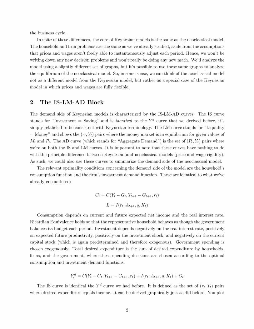
1 Introduction

At the risk of some oversimplification, the leading alternatives to the neoclassical / real business

cycle model for understanding short run fluctuations are Keynesian models. I phrase this in the

plural because there are multiple different versions of the Keynesian model, which differ in terms

of how the aggregate supply block of the economy is formulated. Whereas neoclassical models

emphasize changes in supply as drivers of the business cycle, feature monetary neutrality, and have

no role for activist economic policies, Keynesian models are the opposite – they emphasize demand

changes as the source of business cycles (though changes in supply can also have effects on output),

money is non-neutral, and there is a role for activist stabilization policies.

Though often caricatured as being fundamentally different from the neoclassical model, modern

Keynsian models (which are often called “New Keynesian” models) actually have exactly the same

backbone and structure as the neoclassical model. Agents are optimizing and forward-looking.

There is a well-defined equilibrium concept. The fundamental difference between Keynsian and

neoclassical theories concerns the flexibility of prices and wages. Keynesian theories typically

emphasize nominal rigidities, in the since that the aggregate price level and/or nominal wages may

be imperfectly flexible. This imperfect flexibility of prices and wages (sometimes called price and

wage “stickiness”) can be motivated via the common experience that the prices of the goods we

buy, and the wages we are paid for work, don’t instantaneously change period-to-period in response

to changing conditions. This could be because of things like “menu costs” (it is costly to change

posted prices for some reason), institutional constraints (wage contracts are set in advance and are

difficult to change on the fly), or simply because firms find it costly to pay attention to aggregate

conditions and constantly re-evaluate their prices and wages. Whatever the reason why prices

and/or wages are sticky, this stickiness will do a couple of important things in the model: (i) it

will allow changes in the money supply to have real effects, so that money is non-neutral and (ii)

it will mean that the equilibrium response to other shocks will generally be inefficient, in the sense

of differing from what a fictitious social planner would choose. The fact that the equilibrium will

generally be inefficient gives some justification for activist economic policies designed to stabilize

1

the business cycle.

In spite of these differences, the core of Keynesian models is the same as the neoclassical model.

The household and firm problems are the same as we’ve already studied, aside from the assumptions

that prices and wages aren’t freely able to instantaneously adjust each period. Hence, we won’t be

writing down any new decision problems and won’t really be doing any new math. We’ll analyze the

model using a slightly different set of graphs, but it’s possible to use these same graphs to analyze

the equilibrium of the neoclassical model. So, in some sense, we can think of the neoclassical model

not as a different model from the Keynesian model, but rather as a special case of the Keynesian

model in which prices and wages are fully flexible.

2 The IS-LM-AD Block

The demand side of Keynesian models is characterized by the IS-LM-AD curves. The IS curve

stands for “Investment = Saving” and is identical to the Y d curve that we derived before, it’s

simply relabeled to be consistent with Keynesian terminology. The LM curve stands for “Liquidity

= Money” and shows the (rt, Yt) pairs where the money market is in equilibrium for given values of

Mt and Pt. The AD curve (which stands for “Aggregate Demand”) is the set of (Pt, Yt) pairs where

we’re on both the IS and LM curves. It is important to note that these curves have nothing to do

with the principle difference between Keynesian and neoclassical models (price and wage rigidity).

As such, we could also use these curves to summarize the demand side of the neoclassical model.

The relevant optimality conditions concerning the demand side of the model are the household’s

consumption function and the firm’s investment demand function. These are identical to what we’ve

already encountered:

Ct = C(Yt −Gt, Yt+1 −Gt+1, rt)

It = I(rt, At+1, q,Kt)

Consumption depends on current and future expected net income and the real interest rate.

Ricardian Equivalence holds so that the representative household behaves as though the government

balances its budget each period. Investment depends negatively on the real interest rate, positively

on expected future productivity, positively on the investment shock, and negatively on the current

capital stock (which is again predetermined and therefore exogenous). Government spending is

chosen exogenously. Total desired expenditure is the sum of desired expenditure by households,

firms, and the government, where these spending decisions are chosen according to the optimal

consumption and investment demand functions:

Y dt = C(Yt −Gt, Yt+1 −Gt+1, rt) + I(rt, At+1, q,Kt) +Gt

The IS curve is identical the Y d curve we had before. It is defined as the set of (rt, Yt) pairs

where desired expenditure equals income. It can be derived graphically just as did before. You plot

2

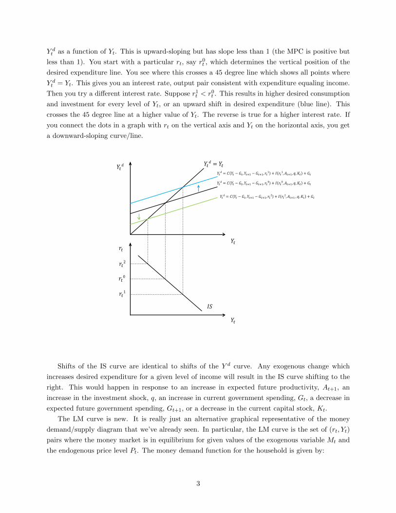
Y dt as a function of Yt. This is upward-sloping but has slope less than 1 (the MPC is positive but

less than 1). You start with a particular rt, say r0t , which determines the vertical position of the

desired expenditure line. You see where this crosses a 45 degree line which shows all points where

Y dt = Yt. This gives you an interest rate, output pair consistent with expenditure equaling income.

Then you try a different interest rate. Suppose r1t < r0t . This results in higher desired consumption

and investment for every level of Yt, or an upward shift in desired expenditure (blue line). This

crosses the 45 degree line at a higher value of Yt. The reverse is true for a higher interest rate. If

you connect the dots in a graph with rt on the vertical axis and Yt on the horizontal axis, you get

a downward-sloping curve/line.

𝑌𝑌𝑡𝑡𝑑𝑑 = 𝐶𝐶 𝑌𝑌𝑡𝑡 − 𝐺𝐺𝑡𝑡,𝑌𝑌𝑡𝑡+1 − 𝐺𝐺𝑡𝑡+1, 𝑟𝑟𝑡𝑡1 + 𝐼𝐼 𝑟𝑟𝑡𝑡1,𝐴𝐴𝑡𝑡+1, 𝑞𝑞,𝐾𝐾𝑡𝑡 + 𝐺𝐺𝑡𝑡

𝑌𝑌𝑡𝑡𝑑𝑑 = 𝑌𝑌𝑡𝑡

𝑌𝑌𝑡𝑡

𝑌𝑌𝑡𝑡

𝑌𝑌𝑡𝑡𝑑𝑑

𝑟𝑟𝑡𝑡

𝑟𝑟𝑡𝑡2

𝑟𝑟𝑡𝑡0

𝑟𝑟𝑡𝑡1

𝐼𝐼𝑆𝑆

𝑌𝑌𝑡𝑡𝑑𝑑 = 𝐶𝐶 𝑌𝑌𝑡𝑡 − 𝐺𝐺𝑡𝑡,𝑌𝑌𝑡𝑡+1 − 𝐺𝐺𝑡𝑡+1, 𝑟𝑟𝑡𝑡0 + 𝐼𝐼 𝑟𝑟𝑡𝑡0,𝐴𝐴𝑡𝑡+1, 𝑞𝑞,𝐾𝐾𝑡𝑡 + 𝐺𝐺𝑡𝑡

𝑌𝑌𝑡𝑡𝑑𝑑 = 𝐶𝐶 𝑌𝑌𝑡𝑡 − 𝐺𝐺𝑡𝑡,𝑌𝑌𝑡𝑡+1 − 𝐺𝐺𝑡𝑡+1, 𝑟𝑟𝑡𝑡2 + 𝐼𝐼 𝑟𝑟𝑡𝑡2,𝐴𝐴𝑡𝑡+1 , 𝑞𝑞,𝐾𝐾𝑡𝑡 + 𝐺𝐺𝑡𝑡

Shifts of the IS curve are identical to shifts of the Y d curve. Any exogenous change which

increases desired expenditure for a given level of income will result in the IS curve shifting to the

right. This would happen in response to an increase in expected future productivity, At+1, an

increase in the investment shock, q, an increase in current government spending, Gt, a decrease in

expected future government spending, Gt+1, or a decrease in the current capital stock, Kt.

The LM curve is new. It is really just an alternative graphical representative of the money

demand/supply diagram that we’ve already seen. In particular, the LM curve is the set of (rt, Yt)

pairs where the money market is in equilibrium for given values of the exogenous variable Mt and

the endogenous price level Pt. The money demand function for the household is given by:

3

Mt = PtMd(rt + πet+1, Yt)

As discussed previously, the demand for money depends on the nominal interest rate. I have

written this in terms of the real interest rate using the approximate Fisher relationship, where we

take expected inflation between t and t + 1, πet+1, to be exogenously given. Since it is exogenous,

most of the time I will treat it as fixed (expected inflation will only change if you are told it is

changing). As such, I will typically write the money demand function omitting explicit dependence

on expected inflation as Mt = PtMd(rt, Yt).

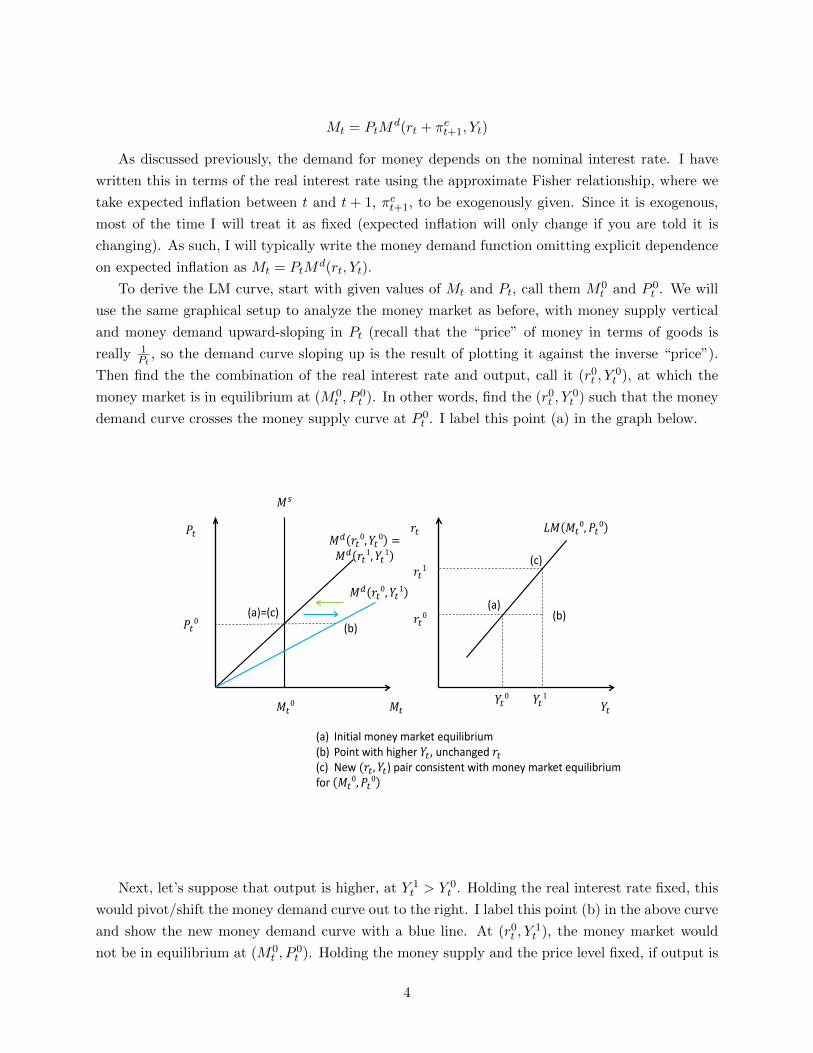
To derive the LM curve, start with given values of Mt and Pt, call them M0t and P 0

t . We will

use the same graphical setup to analyze the money market as before, with money supply vertical

and money demand upward-sloping in Pt (recall that the “price” of money in terms of goods is

really 1Pt

, so the demand curve sloping up is the result of plotting it against the inverse “price”).

Then find the the combination of the real interest rate and output, call it (r0t , Y0t ), at which the

money market is in equilibrium at (M0t , P

0t ). In other words, find the (r0t , Y

0t ) such that the money

demand curve crosses the money supply curve at P 0t . I label this point (a) in the graph below.

𝑀𝑀𝑡𝑡 𝑌𝑌𝑡𝑡

𝑃𝑃𝑡𝑡 𝑟𝑟𝑡𝑡

𝑀𝑀𝑠𝑠

𝑀𝑀𝑑𝑑 𝑟𝑟𝑡𝑡0,𝑌𝑌𝑡𝑡0 = 𝑀𝑀𝑑𝑑 𝑟𝑟𝑡𝑡1,𝑌𝑌𝑡𝑡1

𝑀𝑀𝑡𝑡0

𝑃𝑃𝑡𝑡0

𝑀𝑀𝑑𝑑 𝑟𝑟𝑡𝑡0,𝑌𝑌𝑡𝑡1

𝐿𝐿𝑀𝑀 𝑀𝑀𝑡𝑡0,𝑃𝑃𝑡𝑡0

(a)=(c) (b)

(a) (b)

(c)

(a) Initial money market equilibrium (b) Point with higher 𝑌𝑌𝑡𝑡, unchanged 𝑟𝑟𝑡𝑡 (c) New (𝑟𝑟𝑡𝑡,𝑌𝑌𝑡𝑡) pair consistent with money market equilibrium for 𝑀𝑀𝑡𝑡

0,𝑃𝑃𝑡𝑡0

𝑟𝑟𝑡𝑡0

𝑟𝑟𝑡𝑡1

𝑌𝑌𝑡𝑡0 𝑌𝑌𝑡𝑡1

Next, let’s suppose that output is higher, at Y 1t > Y 0

t . Holding the real interest rate fixed, this

would pivot/shift the money demand curve out to the right. I label this point (b) in the above curve

and show the new money demand curve with a blue line. At (r0t , Y1t ), the money market would

not be in equilibrium at (M0t , P

0t ). Holding the money supply and the price level fixed, if output is

4

higher the real interest rate must adjust in such a way that the money demand curve crosses the

money supply curve at the original point, labeled (a). In other words, rt needs to change in such a

way as to shift the money demand curve in, to undo the outward shift induced by higher Yt. This

mean that rt needs to increase to something like r1t . I label this point (c) in the graph, and at (c)

the quantity of money demand is the same as it was at (a), i.e. Md(r0t , Y0t ) = Md(r1t , Y

1t ). If we

connect the dots in a graph with rt on the vertical axis and Yt on the horizontal axis, we get an

upward-sloping line. This is the LM curve. Mathematically, the LM curve is the set of (rt, Yt) pairs

for which M0t = P 0

t Md(rt, Yt).

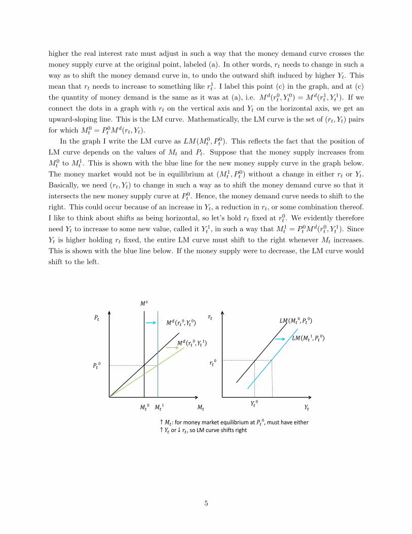
In the graph I write the LM curve as LM(M0t , P

0t ). This reflects the fact that the position of

LM curve depends on the values of Mt and Pt. Suppose that the money supply increases from

M0t to M1

t . This is shown with the blue line for the new money supply curve in the graph below.

The money market would not be in equilibrium at (M1t , P

0t ) without a change in either rt or Yt.

Basically, we need (rt, Yt) to change in such a way as to shift the money demand curve so that it

intersects the new money supply curve at P 0t . Hence, the money demand curve needs to shift to the

right. This could occur because of an increase in Yt, a reduction in rt, or some combination thereof.

I like to think about shifts as being horizontal, so let’s hold rt fixed at r0t . We evidently therefore

need Yt to increase to some new value, called it Y 1t , in such a way that M1

t = P 0t M

d(r0t , Y1t ). Since

Yt is higher holding rt fixed, the entire LM curve must shift to the right whenever Mt increases.

This is shown with the blue line below. If the money supply were to decrease, the LM curve would

shift to the left.



𝑀𝑀𝑠𝑠


𝑀𝑀𝑡𝑡0

𝑃𝑃𝑡𝑡0


↑ 𝑀𝑀𝑡𝑡: for money market equilibrium at 𝑃𝑃𝑡𝑡0, must have either ↑ 𝑌𝑌𝑡𝑡 or ↓ 𝑟𝑟𝑡𝑡, so LM curve shifts right

𝑟𝑟𝑡𝑡0

𝑌𝑌𝑡𝑡0


𝑀𝑀𝑡𝑡1


5

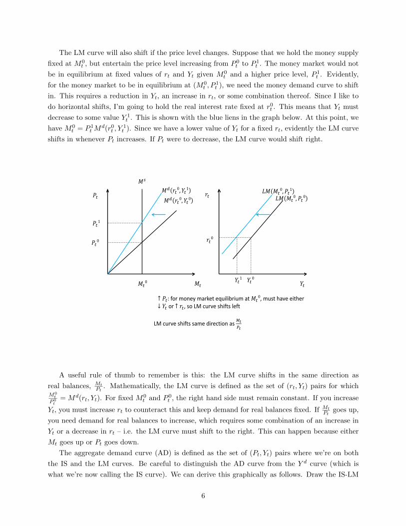
The LM curve will also shift if the price level changes. Suppose that we hold the money supply

fixed at M0t , but entertain the price level increasing from P 0

t to P 1t . The money market would not

be in equilibrium at fixed values of rt and Yt given M0t and a higher price level, P 1

t . Evidently,

for the money market to be in equilibrium at (M0t , P

1t ), we need the money demand curve to shift

in. This requires a reduction in Yt, an increase in rt, or some combination thereof. Since I like to

do horizontal shifts, I’m going to hold the real interest rate fixed at r0t . This means that Yt must

decrease to some value Y 1t . This is shown with the blue liens in the graph below. At this point, we

have M0t = P 1

t Md(r0t , Y

1t ). Since we have a lower value of Yt for a fixed rt, evidently the LM curve

shifts in whenever Pt increases. If Pt were to decrease, the LM curve would shift right.



𝑀𝑀𝑠𝑠


𝑀𝑀𝑡𝑡0

𝑃𝑃𝑡𝑡0

↑ 𝑃𝑃𝑡𝑡: for money market equilibrium at 𝑀𝑀𝑡𝑡0, must have either

↓ 𝑌𝑌𝑡𝑡 or ↑ 𝑟𝑟𝑡𝑡, so LM curve shifts left

𝑟𝑟𝑡𝑡0

𝑌𝑌𝑡𝑡0



𝑃𝑃𝑡𝑡1


𝑌𝑌𝑡𝑡1

LM curve shifts same direction as 𝑀𝑀𝑡𝑡𝑃𝑃𝑡𝑡

A useful rule of thumb to remember is this: the LM curve shifts in the same direction as

real balances, MtPt

. Mathematically, the LM curve is defined as the set of (rt, Yt) pairs for whichM0

t

P 0t

= Md(rt, Yt). For fixed M0t and P 0

t , the right hand side must remain constant. If you increase

Yt, you must increase rt to counteract this and keep demand for real balances fixed. If MtPt

goes up,

you need demand for real balances to increase, which requires some combination of an increase in

Yt or a decrease in rt – i.e. the LM curve must shift to the right. This can happen because either

Mt goes up or Pt goes down.

The aggregate demand curve (AD) is defined as the set of (Pt, Yt) pairs where we’re on both

the IS and the LM curves. Be careful to distinguish the AD curve from the Y d curve (which is

what we’re now calling the IS curve). We can derive this graphically as follows. Draw the IS-LM

6

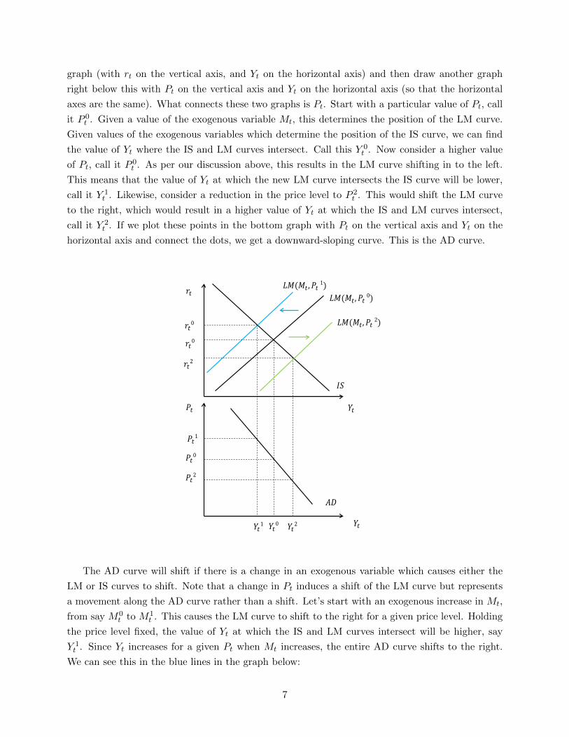
graph (with rt on the vertical axis, and Yt on the horizontal axis) and then draw another graph

right below this with Pt on the vertical axis and Yt on the horizontal axis (so that the horizontal

axes are the same). What connects these two graphs is Pt. Start with a particular value of Pt, call

it P 0t . Given a value of the exogenous variable Mt, this determines the position of the LM curve.

Given values of the exogenous variables which determine the position of the IS curve, we can find

the value of Yt where the IS and LM curves intersect. Call this Y 0t . Now consider a higher value

of Pt, call it P 0t . As per our discussion above, this results in the LM curve shifting in to the left.

This means that the value of Yt at which the new LM curve intersects the IS curve will be lower,

call it Y 1t . Likewise, consider a reduction in the price level to P 2

t . This would shift the LM curve

to the right, which would result in a higher value of Yt at which the IS and LM curves intersect,

call it Y 2t . If we plot these points in the bottom graph with Pt on the vertical axis and Yt on the

horizontal axis and connect the dots, we get a downward-sloping curve. This is the AD curve.

𝐴𝐴𝐴𝐴

𝑌𝑌𝑡𝑡

𝑃𝑃𝑡𝑡 𝑌𝑌𝑡𝑡

𝑟𝑟𝑡𝑡 𝐿𝐿𝐿𝐿(𝐿𝐿𝑡𝑡,𝑃𝑃𝑡𝑡 0)

𝐿𝐿𝐿𝐿(𝐿𝐿𝑡𝑡,𝑃𝑃𝑡𝑡 2)

𝐿𝐿𝐿𝐿(𝐿𝐿𝑡𝑡,𝑃𝑃𝑡𝑡 1)

𝑃𝑃𝑡𝑡0

𝑃𝑃𝑡𝑡2

𝑃𝑃𝑡𝑡1

𝑟𝑟𝑡𝑡0

𝑟𝑟𝑡𝑡2

𝑟𝑟𝑡𝑡0

𝑌𝑌𝑡𝑡0 𝑌𝑌𝑡𝑡2 𝑌𝑌𝑡𝑡1

𝐼𝐼𝐼𝐼

The AD curve will shift if there is a change in an exogenous variable which causes either the

LM or IS curves to shift. Note that a change in Pt induces a shift of the LM curve but represents

a movement along the AD curve rather than a shift. Let’s start with an exogenous increase in Mt,

from say M0t to M1

t . This causes the LM curve to shift to the right for a given price level. Holding

the price level fixed, the value of Yt at which the IS and LM curves intersect will be higher, say

Y 1t . Since Yt increases for a given Pt when Mt increases, the entire AD curve shifts to the right.

We can see this in the blue lines in the graph below:

7

𝐴𝐴𝐴𝐴

𝑌𝑌𝑡𝑡

𝑌𝑌𝑡𝑡

𝑟𝑟𝑡𝑡

𝑃𝑃𝑡𝑡0

𝑟𝑟𝑡𝑡0

𝑌𝑌𝑡𝑡0

𝐴𝐴𝐴𝐴𝐴

𝐼𝐼𝐼𝐼

𝐿𝐿𝐿𝐿 𝐿𝐿𝑡𝑡0,𝑃𝑃𝑡𝑡 0

𝐿𝐿𝐿𝐿 𝐿𝐿𝑡𝑡1,𝑃𝑃𝑡𝑡 0

𝑟𝑟𝑡𝑡1

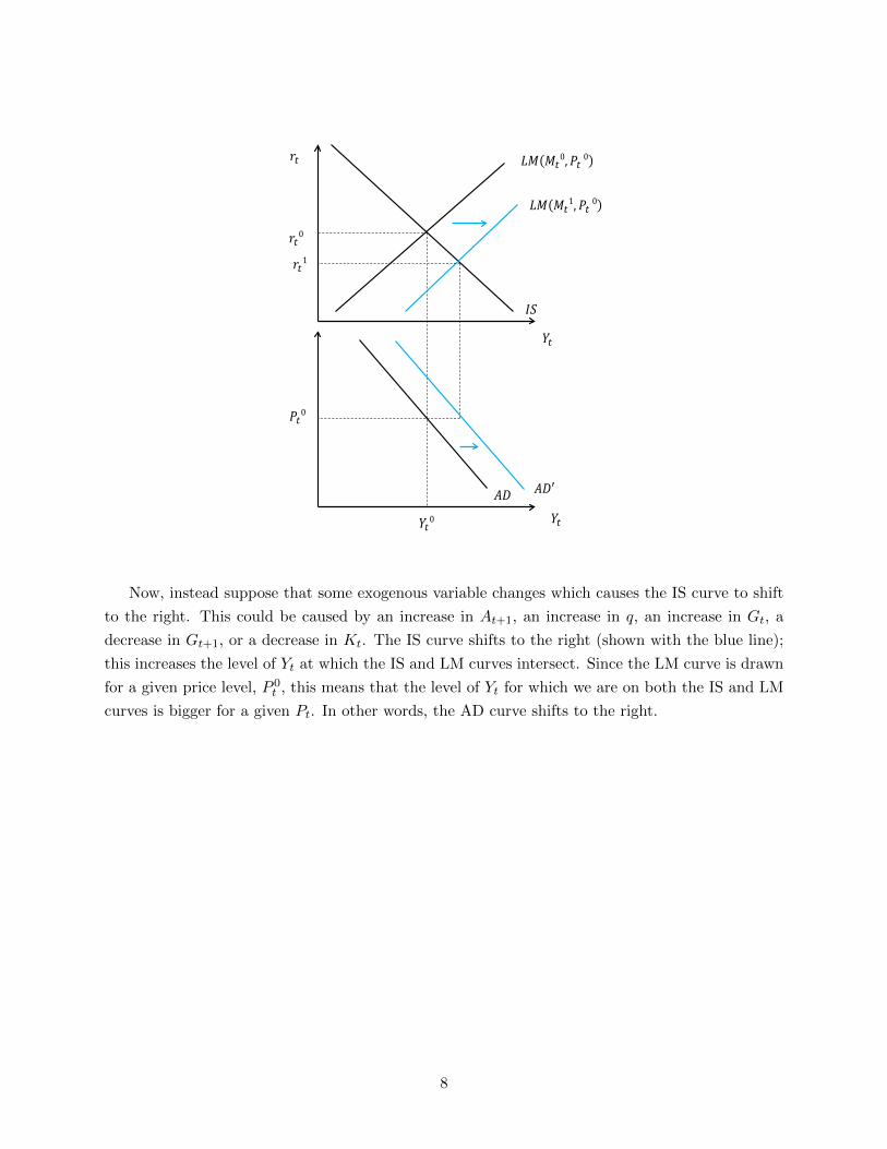
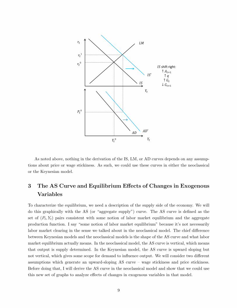
Now, instead suppose that some exogenous variable changes which causes the IS curve to shift

to the right. This could be caused by an increase in At+1, an increase in q, an increase in Gt, a

decrease in Gt+1, or a decrease in Kt. The IS curve shifts to the right (shown with the blue line);

this increases the level of Yt at which the IS and LM curves intersect. Since the LM curve is drawn

for a given price level, P 0t , this means that the level of Yt for which we are on both the IS and LM

curves is bigger for a given Pt. In other words, the AD curve shifts to the right.

8

𝐴𝐴𝐴𝐴

𝑌𝑌𝑡𝑡

𝑌𝑌𝑡𝑡

𝑟𝑟𝑡𝑡

𝑃𝑃𝑡𝑡0

𝑟𝑟𝑡𝑡0

𝑌𝑌𝑡𝑡0

𝐴𝐴𝐴𝐴𝐴

𝐼𝐼𝐼𝐼

𝐿𝐿𝐿𝐿

𝐼𝐼𝐼𝐼𝐴

𝐼𝐼𝐼𝐼 shift right: ↑ 𝐴𝐴𝑡𝑡+1 ↑ 𝑞𝑞 ↑ 𝐺𝐺𝑡𝑡 ↓ 𝐺𝐺𝑡𝑡+1

𝑟𝑟𝑡𝑡1

As noted above, nothing in the derivation of the IS, LM, or AD curves depends on any assump-

tions about price or wage stickiness. As such, we could use these curves in either the neoclassical

or the Keynesian model.

3 The AS Curve and Equilibrium Effects of Changes in Exogenous

Variables

To characterize the equilibrium, we need a description of the supply side of the economy. We will

do this graphically with the AS (or “aggregate supply”) curve. The AS curve is defined as the

set of (Pt, Yt) pairs consistent with some notion of labor market equilibrium and the aggregate

production function. I say “some notion of labor market equilibrium” because it’s not necessarily

labor market clearing in the sense we talked about in the neoclassical model. The chief difference

between Keynesian models and the neoclassical models is the shape of the AS curve and what labor

market equilibrium actually means. In the neoclassical model, the AS curve is vertical, which means

that output is supply determined. In the Keynesian model, the AS curve is upward sloping but

not vertical, which gives some scope for demand to influence output. We will consider two different

assumptions which generate an upward-sloping AS curve – wage stickiness and price stickiness.

Before doing that, I will derive the AS curve in the neoclassical model and show that we could use

this new set of graphs to analyze effects of changes in exogenous variables in that model.

9

3.1 The Neoclassical Model

In the neoclassical model, the supply side of the economy is characterized by a labor demand curve,

a labor supply curve, and the production function. These are:

Nt = N s(wt, Ht)

Nt = Nd(wt, At,Kt)

Yt = AtF (Kt, Nt)

The important thing to note here is that Pt does not appear in any of these expressions. This

means that there is going to be no relationship between Pt and Yt coming from these equations, so

the AS curve will be vertical in a graph with Pt on the vertical axis and Yt on the horizontal axis.

The mathematical equations characterizing the equilibrium of the neoclassical model are the

same as we had before:

Nt = Nd (wt, At,Kt)

Nt = N s(wt, Ht)

Yt = AtF (Kt, Nt)



Yt = Ct + It +Gt

Mt = PtMd(rt, Yt)

This is 7 equations in 7 endogenous variables (Nt, wt, Yt, Ct, It, rt, and Pt). The exogenous

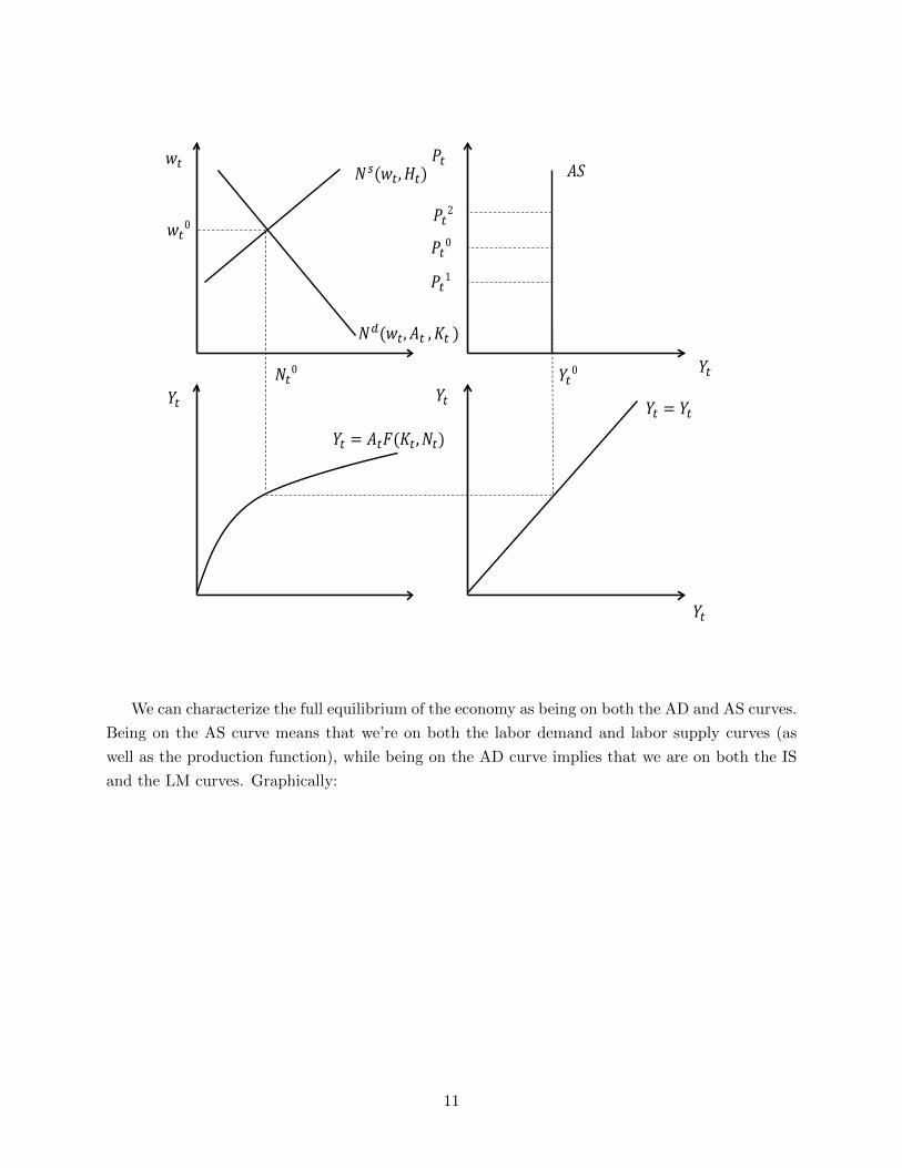
variables are At, At+1, Kt, Gt, Gt+1, q, and Ht. We can graphically characterize the equilibrium

using a similar four part graph to what we had before in the neoclassical model. The labor market

is in the upper left quadrant, the production function is plotted below that, and the bottom right

graph is a 45 degree line reflecting the vertical axis onto the horizontal. The difference relative

to our earlier setup is the graph in the upper right quadrant – now we have a graph with Pt on

the vertical axis and Yt on the horizontal axis (as opposed to rt on the vertical axis). We can

experiment with different values of Pt, but since Pt doesn’t affect the position of the labor demand

or supply curves, nor the position of the production function, we will not get a different value of

Yt for different Pt. So the AS curve will be vertical (just like the Y s curve was vertical, but these

are different concepts). We can see this below.

10

𝑌𝑌𝑡𝑡

𝑤𝑤𝑡𝑡

𝑌𝑌𝑡𝑡

𝑌𝑌𝑡𝑡

𝑌𝑌𝑡𝑡

𝑃𝑃𝑡𝑡

𝑌𝑌𝑡𝑡 = 𝐴𝐴𝑡𝑡𝐹𝐹(𝐾𝐾𝑡𝑡 ,𝑁𝑁𝑡𝑡)

𝑌𝑌𝑡𝑡 = 𝑌𝑌𝑡𝑡

𝑁𝑁𝑑𝑑(𝑤𝑤𝑡𝑡,𝐴𝐴𝑡𝑡 ,𝐾𝐾𝑡𝑡 )

𝑁𝑁𝑠𝑠(𝑤𝑤𝑡𝑡,𝐻𝐻𝑡𝑡) 𝐴𝐴𝐴𝐴

𝑃𝑃𝑡𝑡0

𝑃𝑃𝑡𝑡1

𝑃𝑃𝑡𝑡2 𝑤𝑤𝑡𝑡0

𝑁𝑁𝑡𝑡0 𝑌𝑌𝑡𝑡0

We can characterize the full equilibrium of the economy as being on both the AD and AS curves.

Being on the AS curve means that we’re on both the labor demand and labor supply curves (as

well as the production function), while being on the AD curve implies that we are on both the IS

and the LM curves. Graphically:

11

𝐴𝐴𝐴𝐴

𝐿𝐿𝐿𝐿

𝐼𝐼𝐴𝐴

𝐴𝐴𝐴𝐴

𝑁𝑁𝑠𝑠(𝑤𝑤𝑡𝑡,𝐻𝐻𝑡𝑡)

𝑁𝑁𝑑𝑑(𝑤𝑤𝑡𝑡,𝐴𝐴𝑡𝑡 ,𝐾𝐾𝑡𝑡)


𝑤𝑤𝑡𝑡

𝑌𝑌𝑡𝑡 𝑁𝑁𝑡𝑡 𝑁𝑁𝑡𝑡0

𝑤𝑤𝑡𝑡0

𝑌𝑌𝑡𝑡0

𝑃𝑃𝑡𝑡0

𝑟𝑟𝑡𝑡0

𝑌𝑌𝑡𝑡

𝑌𝑌𝑡𝑡

𝑌𝑌𝑡𝑡


𝑌𝑌𝑡𝑡 𝑃𝑃𝑡𝑡

𝑁𝑁𝑡𝑡

𝑟𝑟𝑡𝑡

This picture graphically determines equilibrium values of Yt, Nt, wt, Pt, and rt. The values of

Ct and It are then determined by looking at the equations underlying the IS curve. In terms of

the equations above, the IS curve summarizes the consumption function, the investment demand

function, and the resource constraint. The LM curve summarizes money demand equaling money

supply. The AD curve encapsulates both the IS and LM curves. The AS curve summarizes the

labor demand and supply curves as well as the production function.

12

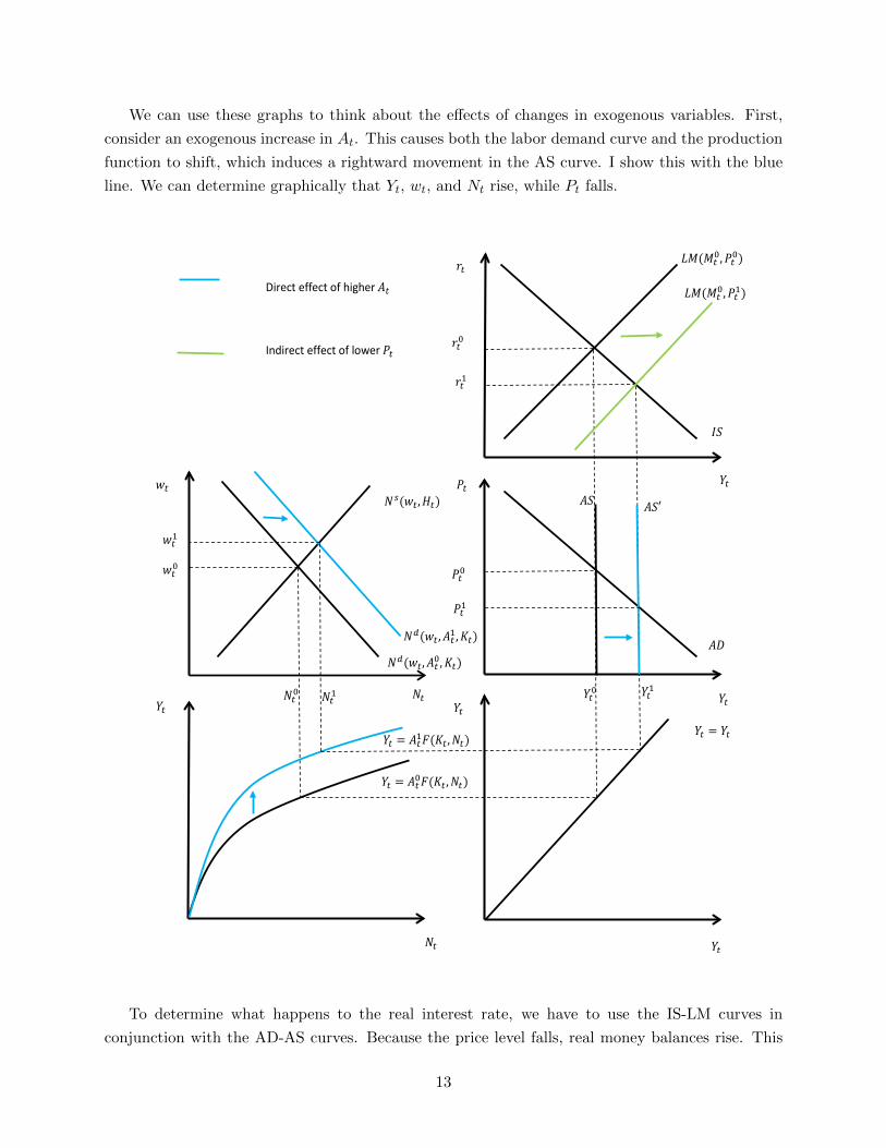
We can use these graphs to think about the effects of changes in exogenous variables. First,

consider an exogenous increase in At. This causes both the labor demand curve and the production

function to shift, which induces a rightward movement in the AS curve. I show this with the blue

line. We can determine graphically that Yt, wt, and Nt rise, while Pt falls.

𝐴𝐴𝐴𝐴

𝐿𝐿𝐿𝐿(𝐿𝐿𝑡𝑡0,𝑃𝑃𝑡𝑡0)

𝐼𝐼𝐴𝐴

𝐴𝐴𝐴𝐴


𝑁𝑁𝑑𝑑(𝑤𝑤𝑡𝑡,𝐴𝐴𝑡𝑡0,𝐾𝐾𝑡𝑡)

𝑌𝑌𝑡𝑡 = 𝐴𝐴𝑡𝑡0𝐹𝐹(𝐾𝐾𝑡𝑡 ,𝑁𝑁𝑡𝑡)

𝑤𝑤𝑡𝑡


𝑤𝑤𝑡𝑡0

𝑌𝑌𝑡𝑡0

𝑃𝑃𝑡𝑡0

𝑟𝑟𝑡𝑡0

𝑌𝑌𝑡𝑡

𝑌𝑌𝑡𝑡

𝑌𝑌𝑡𝑡



𝑁𝑁𝑡𝑡

𝑟𝑟𝑡𝑡


𝐴𝐴𝐴𝐴′


𝑟𝑟𝑡𝑡1

𝑤𝑤𝑡𝑡1

𝑁𝑁𝑡𝑡1

𝑌𝑌𝑡𝑡1

𝑃𝑃𝑡𝑡1


Direct effect of higher 𝐴𝐴𝑡𝑡 Indirect effect of lower 𝑃𝑃𝑡𝑡

To determine what happens to the real interest rate, we have to use the IS-LM curves in

conjunction with the AD-AS curves. Because the price level falls, real money balances rise. This

13

induces a rightward shift of the LM curve. I show that rightward shift in the LM curve with a

green line (to differentiate it from the blue line, where I think of the blue line as representing the

“direct effect” and the green line the “indirect effect” induced by a lower price level). Since the

real interest rate falls and output rises, we can determine that consumption and investment both

rise. Even though it’s not necessarily obvious from these curves, the effects on all the endogenous

variables are identical to what we had in the other graphical setup (you can see this by looking at

the equations).

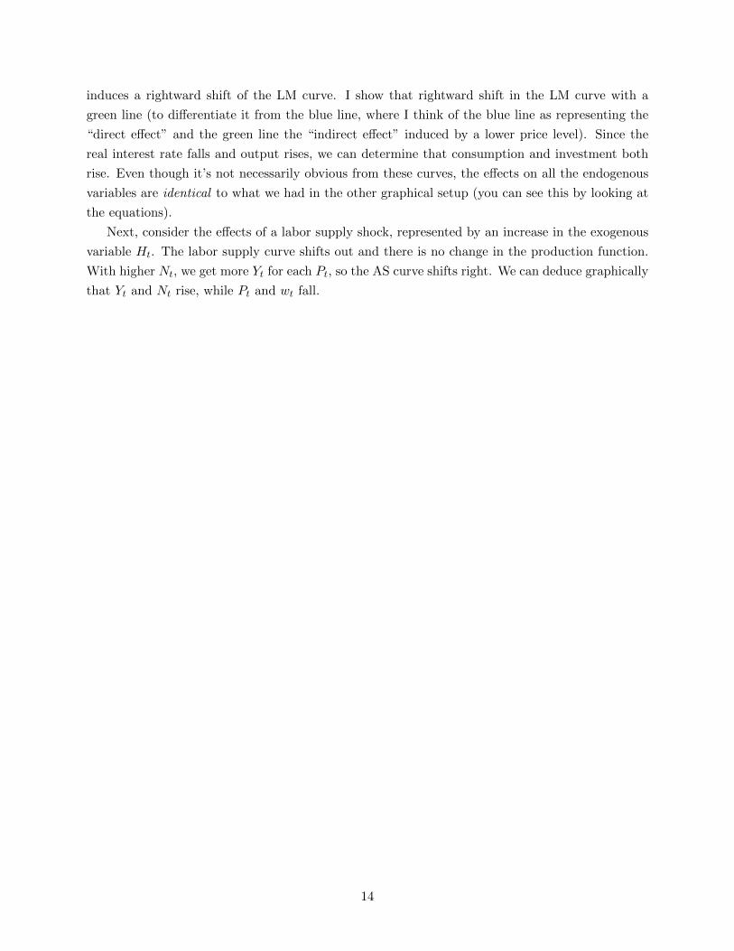
Next, consider the effects of a labor supply shock, represented by an increase in the exogenous

variable Ht. The labor supply curve shifts out and there is no change in the production function.

With higher Nt, we get more Yt for each Pt, so the AS curve shifts right. We can deduce graphically

that Yt and Nt rise, while Pt and wt fall.

14

𝐴𝐴𝐴𝐴


𝐼𝐼𝐴𝐴

𝐴𝐴𝐴𝐴

𝑁𝑁𝑠𝑠(𝑤𝑤𝑡𝑡,𝐻𝐻𝑡𝑡0)



𝑤𝑤𝑡𝑡


𝑤𝑤𝑡𝑡0

𝑌𝑌𝑡𝑡0

𝑃𝑃𝑡𝑡0

𝑟𝑟𝑡𝑡0

𝑌𝑌𝑡𝑡

𝑌𝑌𝑡𝑡

𝑌𝑌𝑡𝑡



𝑁𝑁𝑡𝑡

𝑟𝑟𝑡𝑡


𝐴𝐴𝐴𝐴′


𝑟𝑟𝑡𝑡1

𝑤𝑤𝑡𝑡1

𝑁𝑁𝑡𝑡1

𝑌𝑌𝑡𝑡1

𝑃𝑃𝑡𝑡1

Direct effect of higher 𝐻𝐻𝑡𝑡 Indirect effect of lower 𝑃𝑃𝑡𝑡


To determine the effect on the real interest rate, we have to use the IS-LM curves in conjunction

with the AD-AS curves. The lower price level induces a rightward shift in the LM curve, denoted

by the green line. This results in a lower real interest rate. Since the real interest rate is lower and

output is higher, both consumption and investment are higher. The changes in the endogenous

variables are again identical to what we had before in the different graphical setup.

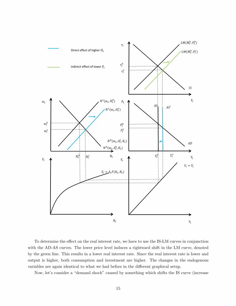
Now, let’s consider a “demand shock” caused by something which shifts the IS curve (increase

15

in At+1, q, or Gt, or decrease in Gt+1 or Kt). This is shown with the blue line in the IS-LM

diagram. This causes the AD curve to shift out. Given the vertical AS curve, this results in no

change in Yt, wt, or Nt, but an increase in Pt. The increase in Pt causes the LM curve to shift in.

This is shown with the green line. Since there is no change in Yt from the AD-AS intersection, the

LM curve shifts in such that it intersects the new IS curve at the original level of Yt with a higher

rt. How consumption and investment are affected depends on which exogenous variable triggered

the shift in the IS curve. The effects are identical to what we saw before.

𝐴𝐴𝐴𝐴


𝐼𝐼𝐴𝐴

𝐴𝐴𝐴𝐴




𝑤𝑤𝑡𝑡


𝑤𝑤𝑡𝑡0

𝑌𝑌𝑡𝑡0

𝑃𝑃𝑡𝑡0

𝑟𝑟𝑡𝑡0

𝑌𝑌𝑡𝑡

𝑌𝑌𝑡𝑡

𝑌𝑌𝑡𝑡



𝑁𝑁𝑡𝑡

𝑟𝑟𝑡𝑡

𝑃𝑃𝑡𝑡1

𝑟𝑟𝑡𝑡1

𝐼𝐼𝐴𝐴′

𝐴𝐴𝐴𝐴′


Direct effect of IS shock Indirect effect of higher 𝑃𝑃𝑡𝑡

16

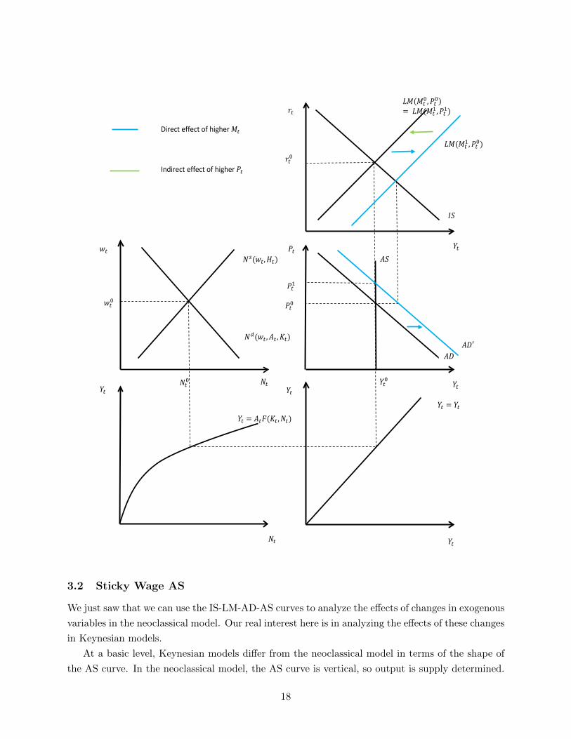
Finally, consider the effect of an exogenous increase in the money supply, from M0t to M1

t . This

causes the LM curve to shift right, which induces a rightward shift in the AD curve. These are

shown with the blue lines in the diagram below. Since the AS curve is vertical, there is no change in

Yt and an increase in Pt. There is no effect on either wt or Nt. The higher Pt causes the LM curve

to shift in. Since there is no change in Yt from the AD-AS intersection, this evidently means that

the increase in Pt is sufficient to completely “undo” the rightward shift of the LM curve, so that on

net, there is no shift in the LM curve, and hence no change in rt. Mathematically this means that

LM(M0t , P

0t ) = LM(M1

t , P1t ), which means that there is no effect on real balances; in other words,

MtPt

does not change, so that the price level simply rises proportionately with the money supply.

Since neither rt nor Yt change, there are no changes in consumption or investment. There are no

real effects of a change in the money supply, so money is neutral, just as we saw before.

17

𝐴𝐴𝐴𝐴

𝐼𝐼𝐴𝐴

𝐴𝐴𝐴𝐴




𝑤𝑤𝑡𝑡


𝑤𝑤𝑡𝑡0

𝑌𝑌𝑡𝑡0

𝑃𝑃𝑡𝑡0

𝑟𝑟𝑡𝑡0

𝑌𝑌𝑡𝑡

𝑌𝑌𝑡𝑡

𝑌𝑌𝑡𝑡



𝑁𝑁𝑡𝑡

𝑟𝑟𝑡𝑡 𝐿𝐿𝐿𝐿(𝐿𝐿𝑡𝑡

0,𝑃𝑃𝑡𝑡0)= 𝐿𝐿𝐿𝐿(𝐿𝐿𝑡𝑡

1,𝑃𝑃𝑡𝑡1)


𝑃𝑃𝑡𝑡1

𝐴𝐴𝐴𝐴′

Direct effect of higher 𝐿𝐿𝑡𝑡 Indirect effect of higher 𝑃𝑃𝑡𝑡

3.2 Sticky Wage AS

We just saw that we can use the IS-LM-AD-AS curves to analyze the effects of changes in exogenous

variables in the neoclassical model. Our real interest here is in analyzing the effects of these changes

in Keynesian models.

At a basic level, Keynesian models differ from the neoclassical model in terms of the shape of

the AS curve. In the neoclassical model, the AS curve is vertical, so output is supply determined.

18

In Keynesian models, the AS curve is upward sloping but not vertical, so there is some role for

demand. To get the AS upward sloping we have to assume some sort of different structure on the

supply side of the economy. The two most popular and straightforward structures are sticky wages

and sticky prices. In this subsection we derive the sticky wage AS curve and then examine how the

economy reacts to changes in the different exogenous variables.

In the sticky wage model we assume that the nominal wage, Wt, is fixed at some exogenous

value, W . You can think of this as being set in advance and unable to change in response to

exogenous variables within a period, t. The real wage is wt = WtPt

or WPt

. The mathematical

equations characterizing the supply side of the labor market are the same as before, though we

have an extra condition determining the real wage in terms of the fixed nominal wage and the price

level:

Nt = N s (wt, Ht)

Nt = Nd (wt, At,Kt)

Yt = AtF (Kt, Nt)

wt =W

Pt

With the nominal wage fixed, it’s going to generally be impossible for the labor market to clear

in the way we’ve defined it before. Why is this? Suppose that the price level, Pt, increases. With

a fixed nominal wage, this reduces the real wage. This makes firms want to hire more labor (labor

demand is downward-sloping in the real wage) but makes households want to work less (labor

supply is increasing in the real wage). We are going to make the following assumption: we are

going to assume that the quantity of labor is determined from the labor demand curve, so we are

not necessarily on the labor supply curve. I will typically draw these graphs where W is set such

that we would simultaneously be on both labor demand and labor supply given exogenous variables,

but when an exogenous variable changes we will determine labor from the labor demand curve. In

this sense labor demand need not equal labor supply in equilibrium.1 Mathematically, this involves

essentially replacing the labor supply curve with the definition of the real wage in terms of the fixed

nominal wage and the price level.

The mathematical equations characterizing the equilibrium of the sticky wage Keynesian model

are therefore:

Nt = Nd (wt, At,Kt)

1One might question how firms could force workers to work more than they might otherwise want to. One couldmotivate this via an attachment story – a household may not want to work off of its labor supply curve, but if thehousehold is somehow attached to the firm it may be willing to do so at least for a while so as to avoid gettingfired and not having a job in the future. An alternative way to address this problem would be to assume that W isalways set such that real wage, W

Ptis always above the labor market clearing real wage (so that the quantity of labor

supplied exceeds quantity demanded at the real wage). Reading quantity off the labor demand curve, the householdis working less than it would otherwise like to, so the household would be willing to work more in response to a shockif the firm wants to hire more.

19

wt =W

Pt

Yt = AtF (Kt, Nt)



Yt = Ct + It +Gt

Mt = PtMd(rt, Yt)

Just as in the neoclassical model, this is again 7 equations in 7 endogenous variables (Nt, wt,

Yt, Ct, It, rt, and Pt). What is different than the neoclassical model is that we have replaced the

labor supply curve with the condition wt = WPt

, and have included W as a new exogenous variable.

So in a very basic sense, really all we’ve changed relative to the neoclassical model is that we’ve

replaced the labor supply curve with a condition determining the real wage as a function of the

price level given the fixed nominal wage.

We graphically derive an AS curve in a way similar to what we did before in a four part graph.

Unlike in the neoclassical model, here there is a connection between the price level and the supply

side of the model through the effect of the price level on the real wage, given the fixed nominal

wage. Start with a value of Pt in the upper right quadrant, call it P 0t . For ease of exposition,

suppose that given this value of the price level W is such that the labor market clears at wt = WP 0t

in the sense that we’re simultaneously on both the labor demand and supply curves. Given the real

wage WP 0t

, we determine Nt from the labor demand curve. Then we plug that Nt into the aggregate

production function (the lower left graph), which then gives us a value of Yt. Reflecting this over

using the 45 degree line in the lower right quadrant, we get a (Pt, Yt) pair. Now, consider a lower

value of the price level, P 1t . A lower price level means that the real wage increases because the

nominal wage is fixed. This effectively causes firms to move “up” the labor demand curve – with

a higher real wage, firms want to hire less labor. Less labor plugged into the production function

means less output. So we get a new (Pt, Yt) pair that is to the “southwest” of the original pair.

Connecting the dots, we get an upward-sloping (but not vertical) AS curve.2

2Note that in the sticky wage model we are always on the labor demand curve but not on the labor supply curve.As we will see, the reverse will be true in the sticky price model. This permits there to be differences betweenthe quantity of labor supplied and the quantity demanded. If the quantity of labor supplied exceeds the quantitydemanded, this sounds a lot like unemployment as it is defined in the data (people who are unemployed are thosewho would like to work but cannot find work). This is an interpretation one can give to these models but we will notfocus on it, instead focusing on the behavior of aggregate output and aggregate labor input.

20

𝑌𝑌𝑡𝑡

𝑤𝑤𝑡𝑡

𝑌𝑌𝑡𝑡

𝑌𝑌𝑡𝑡

𝑌𝑌𝑡𝑡

𝑃𝑃𝑡𝑡



𝑁𝑁𝑑𝑑(𝑤𝑤𝑡𝑡,𝐴𝐴𝑡𝑡 ,𝐾𝐾𝑡𝑡 )


𝑊𝑊� 𝑃𝑃𝑡𝑡0⁄

𝑊𝑊� 𝑃𝑃𝑡𝑡1⁄ 𝐴𝐴𝐴𝐴

𝑃𝑃𝑡𝑡0

𝑃𝑃𝑡𝑡1

The IS-LM-AD block is unaffected by wage stickiness. So we can simply draw in the AD curve

and look at the IS-LM curves to fully characterize the equilibrium.

21

𝐴𝐴𝐴𝐴

𝐿𝐿𝐿𝐿

𝐼𝐼𝐴𝐴

𝐴𝐴𝐴𝐴




𝑤𝑤𝑡𝑡



𝑌𝑌𝑡𝑡0

𝑃𝑃𝑡𝑡0

𝑟𝑟𝑡𝑡0

𝑌𝑌𝑡𝑡

𝑌𝑌𝑡𝑡

𝑌𝑌𝑡𝑡



𝑁𝑁𝑡𝑡

𝑟𝑟𝑡𝑡

The IS curve summarizes the consumption function, the investment demand function, and the

the resource constraint. The LM curve summarizes the condition that money demand equals supply

(which is given exogenously). The AS curve summarizes the labor demand curve, the production

function, the condition that the real wage equals the fixed nominal wage divided by the price level.

We can consider the effects of changes in exogenous variables in this model in a conceptually

similar manner to what we did before, but the answers are going to be different. Let’s start with

22

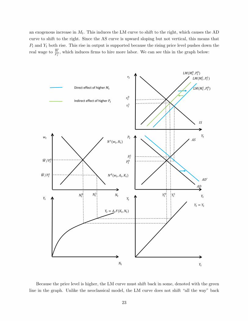
an exogenous increase in Mt. This induces the LM curve to shift to the right, which causes the AD

curve to shift to the right. Since the AS curve is upward sloping but not vertical, this means that

Pt and Yt both rise. This rise in output is supported because the rising price level pushes down the

real wage to WP 1t

, which induces firms to hire more labor. We can see this in the graph below:

𝐴𝐴𝐴𝐴


𝐼𝐼𝐴𝐴

𝐴𝐴𝐴𝐴




𝑤𝑤𝑡𝑡



𝑌𝑌𝑡𝑡0

𝑃𝑃𝑡𝑡0

𝑟𝑟𝑡𝑡0

𝑌𝑌𝑡𝑡

𝑌𝑌𝑡𝑡

𝑌𝑌𝑡𝑡



𝑁𝑁𝑡𝑡

𝑟𝑟𝑡𝑡

𝑌𝑌𝑡𝑡1


𝑟𝑟𝑡𝑡1

𝑃𝑃𝑡𝑡1

𝑁𝑁𝑡𝑡1




𝐴𝐴𝐴𝐴′

Because the price level is higher, the LM curve must shift back in some, denoted with the green

line in the graph. Unlike the neoclassical model, the LM curve does not shift “all the way” back

23

in since Yt is higher. In other words, relative to the neoclassical model with a vertical AS curve,

the price level does not rise as much, so that real balances, MtPt

, increase, and the LM curve “on

net” shifts right. This means that the real interest rate is lower. A lower real interest rate plus

higher output means that both consumption and investment are higher. Working back to the labor

market, a higher price level with an unchanged nominal wage means that the real wage is lower.

The lower real wage causes firms to hire more labor, so Nt increases and wt decreases.

Hence, by increasing the money supply a central bank can lower the real interest rate in this

model, which stimulates both investment and consumption. A lower real interest rate as the

“monetary transmission” mechanism is loosely how people in the real world think about the real

effects of monetary policy – central banks are able to manipulate interest rates through their control

of the money supply, which induces changes in consumption and investment. What is critical for

this to happen in this model is that there is a friction (in this case, the nominal wage being sticky)

which keeps the price level from rising as much as it would as in the neoclassical model.

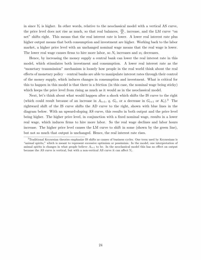
Next, let’s think about what would happen after a shock which shifts the IS curve to the right

(which could result because of an increase in At+1, q, Gt, or a decrease in Gt+1 or Kt).3 The

rightward shift of the IS curve shifts the AD curve to the right, shown with blue lines in the

diagram below. With an upward-sloping AS curve, this results in both output and the price level

being higher. The higher price level, in conjunction with a fixed nominal wage, results in a lower

real wage, which induces firms to hire more labor. So the real wage declines and labor hours

increase. The higher price level causes the LM curve to shift in some (shown by the green line),

but not so much that output is unchanged. Hence, the real interest rate rises.

3Traditional Keynesian theories emphasize IS shifts as causes of business cycles. One term used by Keynesians is“animal spirits,” which is meant to represent excessive optimism or pessimism. In the model, one interpretation ofanimal spirits is changes in what people believe At+1 to be. In the neoclassical model this has no effect on outputbecause the AS curve is vertical, but with a non-vertical AS curve it can affect Yt.

24

𝐴𝐴𝐴𝐴


𝐼𝐼𝐴𝐴

𝐴𝐴𝐴𝐴




𝑤𝑤𝑡𝑡



𝑌𝑌𝑡𝑡0

𝑃𝑃𝑡𝑡0

𝑟𝑟𝑡𝑡0

𝑌𝑌𝑡𝑡

𝑌𝑌𝑡𝑡

𝑌𝑌𝑡𝑡



𝑁𝑁𝑡𝑡

𝑟𝑟𝑡𝑡

𝑌𝑌𝑡𝑡1


𝑟𝑟𝑡𝑡1

𝑃𝑃𝑡𝑡1

𝑁𝑁𝑡𝑡1



𝐼𝐼𝐴𝐴′

𝐴𝐴𝐴𝐴′

We cannot determine what happens to Ct or It without knowing what exogenous variable

changed in the first place. Suppose that the IS shock were caused by an increase in expected future

productivity, At+1. As in the neoclassical model, it would be ambiguous as to what happens to

both Ct and It – higher At+1 works to make both of these higher and higher Yt works to make Ct

higher, other things being equal, while higher rt works to make both Ct and It lower. Hence, the

effect of higher At+1 on these variables is ambiguous.

25

Suppose instead that the IS shock were caused by an increase in q. Higher q has a direct

effect that makes It higher, but higher rt has the effect of working to make It lower. However,

we actually know that It must be higher in the new equilibrium. Why is that? We argued that

in the neoclassical model It would be higher when q goes up, or that the direct effect dominates.

In the sticky wage Keynesian model, the increase in rt after an increase in q is smaller than in

the neoclassical model (you can see this by noting that the neoclassical model is a special case of

this model with a vertical AS curve). Hence, the indirect effect due to the higher interest rate is

even smaller than in the neoclassical model, so we know that It must rise. What happens to Ct is

ambiguous – higher Yt works to make consumption bigger, while higher rt has the opposite effect.

We cannot definitely determine what happens to Ct here.

Suppose that the IS shock were caused by an increase in Gt. This makes rt higher, which means

that It will be lower. Higher rt works to make Ct lower, higher Gt works to make Ct lower, but

higher Yt works to make Ct higher. Hence, it seems that the effect on Ct is ambiguous. But it turns

out it’s not. Back in the equilibrium in an endowment economy material, we argued that output

would increase one-for-one with Gt if the real interest rate were held fixed – in the terminology

of this new model, the magnitude of the horizontal shift in the IS curve is equal to the change in

Gt. But since the real interest rate rises in the new equilibrium, the actual change in output is

smaller than the change in Gt. Put another way, in this model the government spending multiplier

is positive (unlike zero in the neoclassical model), but less than one. Since Yt goes up by less than

Gt, Yt − Gt goes down, so perceived current net income falls. Falling current net income exerts

a negative effect on consumption. Combined with the higher real interest rate, this means that

consumption falls after an increase in Gt.

Suppose that the IS shock were caused by an expected reduction in future government spending.

Since the real interest rate rises and nothing else relevant for investment has changed, we can deduce

that It must fall. But since Yt is higher and current Gt is unchanged, for Yt to rise and It to fall it

must be the case that Ct rises.

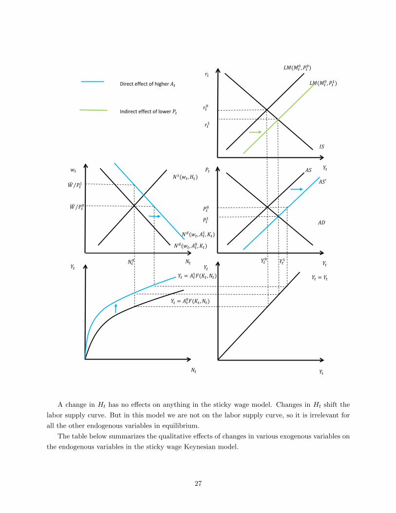
Next, let’s consider the effects of an increase in At in the sticky wage model. The higher At

has two direct effects – it shifts the labor demand curve to the right, and it shifts the production

function up. Holding the price level fixed, labor demand shifting right would result in higher Nt.

Higher Nt plus higher At means higher Yt for a given Pt. In other words, the AS curve shifts to

the right. This means that Yt rises and Pt falls. The fall in Pt induces an outward shift of the

LM curve (shown by the green line), so that rt falls. rt falling with Yt rising means that both

consumption and investment also rise. We have to work our way back to the labor market. The

lower Pt results in a higher real wage, which induces firms to hire less labor. In this model, it turns

out to be ambiguous how Nt reacts – it could be higher, lower, or unchanged. In the picture below

I’ve drawn it as being unchanged, but in general it is ambiguous. We will return to this point in

some more detail later.

26

𝐴𝐴𝐴𝐴


𝐼𝐼𝐴𝐴

𝐴𝐴𝐴𝐴




𝑤𝑤𝑡𝑡



𝑌𝑌𝑡𝑡0

𝑃𝑃𝑡𝑡0

𝑟𝑟𝑡𝑡0

𝑌𝑌𝑡𝑡

𝑌𝑌𝑡𝑡

𝑌𝑌𝑡𝑡



𝑁𝑁𝑡𝑡

𝑟𝑟𝑡𝑡




𝑟𝑟𝑡𝑡1

𝐴𝐴𝐴𝐴′

𝑃𝑃𝑡𝑡1

𝑌𝑌𝑡𝑡1



A change in Ht has no effects on anything in the sticky wage model. Changes in Ht shift the

labor supply curve. But in this model we are not on the labor supply curve, so it is irrelevant for

all the other endogenous variables in equilibrium.

The table below summarizes the qualitative effects of changes in various exogenous variables on

the endogenous variables in the sticky wage Keynesian model.

27

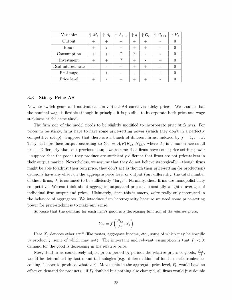
Variable: ↑ Mt ↑ At ↑ At+1 ↑ q ↑ Gt ↑ Gt+1 ↑ Ht

Output + + + + + - 0

Hours + ? + + + - 0

Consumption + + ? ? - - 0

Investment + + ? + - + 0

Real interest rate - - + + + - 0

Real wage - + - - - + 0

Price level + - + + + - 0

3.3 Sticky Price AS

Now we switch gears and motivate a non-vertical AS curve via sticky prices. We assume that

the nominal wage is flexible (though in principle it is possible to incorporate both price and wage

stickiness at the same time).

The firm side of the model needs to be slightly modified to incorporate price stickiness. For

prices to be sticky, firms have to have some price-setting power (which they don’t in a perfectly

competitive setup). Suppose that there are a bunch of different firms, indexed by j = 1, . . . , J .

They each produce output according to Yj,t = AtF (Kj,t, Nj,t), where At is common across all

firms. Differently than our previous setup, we assume that firms have some price-setting power

– suppose that the goods they produce are sufficiently different that firms are not price-takers in

their output market. Nevertheless, we assume that they do not behave strategically – though firms

might be able to adjust their own price, they don’t act as though their price-setting (or production)

decisions have any effect on the aggregate price level or output (put differently, the total number

of these firms, J , is assumed to be sufficiently “large”. Formally, these firms are monopolistically

competitive. We can think about aggregate output and prices as essentially weighted-averages of

individual firm output and prices. Ultimately, since this is macro, we’re really only interested in

the behavior of aggregates. We introduce firm heterogeneity because we need some price-setting

power for price-stickiness to make any sense.

Suppose that the demand for each firm’s good is a decreasing function of its relative price:

Yj,t = f

(Pj,t

Pt, Xj

)Here Xj denotes other stuff (like tastes, aggregate income, etc., some of which may be specific

to product j, some of which may not). The important and relevant assumption is that f1 < 0:

demand for the good is decreasing in the relative price.

Now, if all firms could freely adjust prices period-by-period, the relative prices of goods,Pj,t

Pt,

would be determined by tastes and technologies (e.g. different kinds of foods, or electronics be-

coming cheaper to produce, whatever). Movements in the aggregate price level, Pt, would have no

effect on demand for products – if Pt doubled but nothing else changed, all firms would just double

28

their prices, Pj,t. This wouldn’t change relative prices, so there would be no change in the demand

for goods, and hence there would be no effect of a change in Pt on total output – money would be

“neutral” as it is in the benchmark neoclassical model.

Suppose instead that firms have to set their prices in advance based on what they expect the

aggregate price level to be. Denote the aggregate expected price level as P et . We take this variable

to be exogenous. Each individual firm sets its own price to target an optimal relative price based

on other conditions specific to its product. Suppose that some fraction of firms cannot adjust

their price within period to changes in the aggregate price level, say because of “menu costs” or

informational frictions. This means that an increase in the aggregate price level, Pt, over and above

what was expected, P et , will lead these firms to have relative prices that are too low (while firms

that can update their prices will have their target relative prices). With a lower relative price,

there will be more demand for these goods. The “rules of the game” are that a firm must produce

however much output is demanded at its price – the rational for which could be that refusing to

produce so as to meet demand would lead to a loss in customer loyalty (or something similar).

Therefore, having a suboptimally low relative price means that a firm that cannot adjust its own

price must produce more when the aggregate price level is higher than was expected. With some

firms producing more than they would like to, aggregate output will rise. Thus, there will be a

positive relationship between surprise changes in the price level and the level of economic activity.

Let Y ft denote the hypothetical amount of output that would be produced in the neoclassical

model where prices are flexible (hence the f superscript). This is unaffected by price rigidities –

it would be the equilibrium level of output given the real exogenous variables (At, At+1, Gt, Gt+1,

Kt, q, and Ht) in the model where there were no pricing rigidities. Let Yt denote the actual amount

produced. Our story above says that when the aggregate price level increases, output increases,

because some firms cannot/don’t adjust their own price, and hence end up producing more than

they find optimal. The story from the above paragraph suggests that there ought to be a positive

relationship between the gap between Yt and Y ft and the gap between the actual and expected

price level – the actual price level being higher than expected leads to more production than would

take place without price rigidity, whereas the price level being lower than expected leads to less

production. We therefore suppose that the aggregate price-output dynamics obey the following

Aggregate Supply (AS) relationship:

Pt = P et + γ(Yt − Y f

t )

0 ≤ γ ≤ ∞ is a parameter tells us how “sticky” prices are (in essence the fraction of firms than

are unable to adjust their price). If γ →∞, then prices are perfectly flexible: we’d have Yt = Y ft ,

even if Pt 6= P et . If the aggregate price level differs from what was expected, but if all firms can

adjust prices freely, then all will do so with no change in relative prices at the micro level. In

contrast, if γ → 0, then this conforms with all firms having sticky prices – if no firms can adjust

their price within period, then the aggregate price level will be equal to what it was expected to

equal (the aggregate price level cannot change within period – it is fixed if all firms are unable to

29

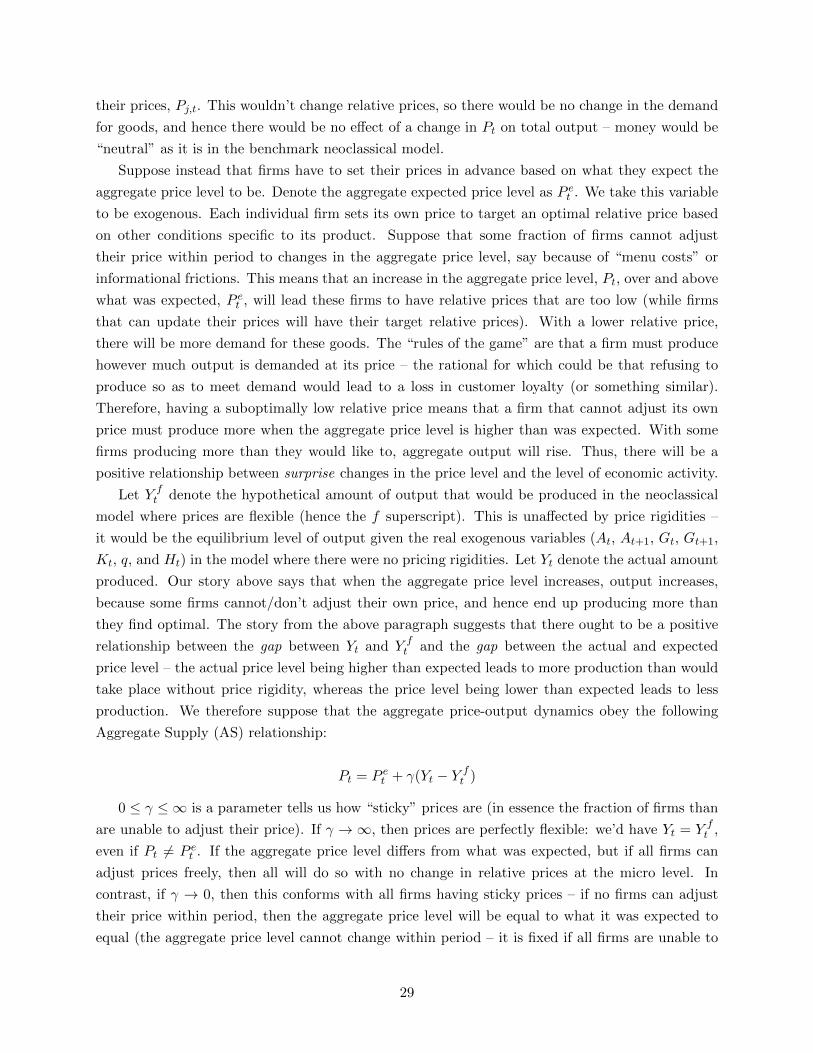
adjust their price). For intermediate cases between γ → 0 and γ →∞, the AS curve will be upward

sloping in a graph with Yt on the horizontal axis and Pt on the vertical axis. When Yt = Y ft , we

will have Pt = P et (except in the case in which the AS Curve is perfectly vertical, with γ →∞).

𝑌𝑌𝑡𝑡

𝑃𝑃𝑡𝑡

𝐴𝐴𝐴𝐴

𝐴𝐴𝐴𝐴(𝛾𝛾 𝑠𝑠𝑠𝑠𝑠𝑠𝑠𝑠𝑠𝑠)

𝐴𝐴𝐴𝐴(𝛾𝛾 𝑠𝑠𝑠𝑠𝑙𝑙𝑙𝑙𝑙𝑙)

AS: 𝑃𝑃𝑡𝑡 = 𝑃𝑃𝑡𝑡𝑒𝑒 + 𝛾𝛾(𝑌𝑌𝑡𝑡 − 𝑌𝑌𝑡𝑡𝑓𝑓)

𝑃𝑃𝑡𝑡𝑒𝑒

𝑌𝑌𝑡𝑡𝑓𝑓

The figure above plots the AS curve. Regardless of the value of γ, the AS curve must cross

through the point (P et , Y

ft ) – when Pt = P e

t , for the AS curve to hold it must be the case that

Yt = Y ft . I show three different variants of the AS curve corresponding to different values of γ.

The black line shows the AS curve for an “intermediate” value of γ. The orange line shows the AS

curve for a large value of γ – a large value of γ corresponds to not many firms having sticky prices,

and in the limit as γ →∞ the AS curve is identical to what you get in the neoclassical model. The

blue line shows the AS curve for a small value of γ, which corresponds to prices being quite sticky

and the AS curve consequently being relatively flat.

The aggregate production function is the same as it has been before, and is identical to the

individual firm production functions:4

Yt = AtF (Kt, Nt)

The desired aggregate labor demand for firms is also the same as it was before:

Nt = Nd(wt, At,Kt)

I put the word “desired” in italics above because this curve ends up being irrelevant for the

determination of aggregate employment. Why is that? As mentioned above, the “rules of the game”

4All the firms have the same form of the production function but may employ different quantities of capital andlabor. Under fairly weak assumptions we can aggregate the individual firm production functions to yield an identicalaggregate production function to what we had in the flexible price model. You do not need to worry about this.

30

are that the firms produce however much is demanded at their relative price. If the actual price

level is higher than firms expected, some firms have suboptimally low relative prices, which means

they have to produce more than they would like to if they were maximizing profits. Therefore,

firms are required to hire sufficient labor to produce however much is demanded at their price and

must produce more than they would otherwise like if prices were flexible. This means that they

are in general off their labor demand curve. The equilibrium concept in the labor market is that

the real wage and the level of employment are determined from the household’s labor supply curve,

given the level of Yt consistent with being on both the AD and AS curves. If you compare this to

the sticky wage model, an easy way to remember this is that we’re on the labor supply curve in the

sticky price model (but not necessarily the labor demand curve), while we’re on the labor demand

curve in the sticky wage model (but not necessarily the labor supply curve).

The household side of the model is identical to what we’ve had before. The consumption

function, investment demand function, and labor supply function are:



Nt = N s(wt, Ht)

The full set of equations characterizing the equilibrium is given below:

Pt = P et + γ(Yt − Y f

t )

Nt = N s(wt, Ht)

Yt = AtF (Kt, Nt)



Yt = Ct + It +Gt

Mt = PtMd(rt, Yt)

Just as in the neoclassical and sticky wage Keynesian models, this is 7 equations in 7 endogenous

variables. Relative to the neoclassical model, we have replaced the labor demand curve with the

AS curve Pt = P et + γ(Yt − Y f

t ). P et is taken to be exogenous and Y f

t is what output would equal

if prices were flexible (i.e. what output would equal in he neoclassical model). So just like as in

the sticky wage Keynesian model, relative to the neoclassical model we’re just swapping out one

equation with a new one (in this case, the labor demand curve with the AS relationship above; in

the sticky wage model, the labor supply curve with the condition determining the real wage given

the nominal wage).

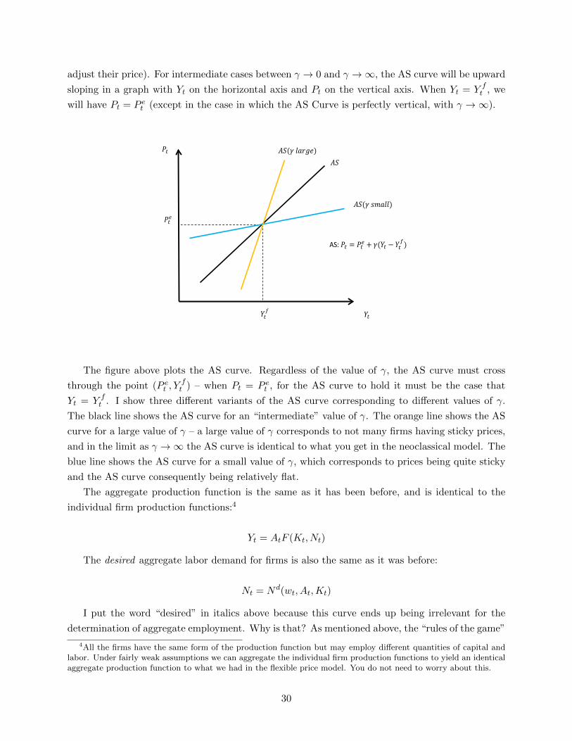
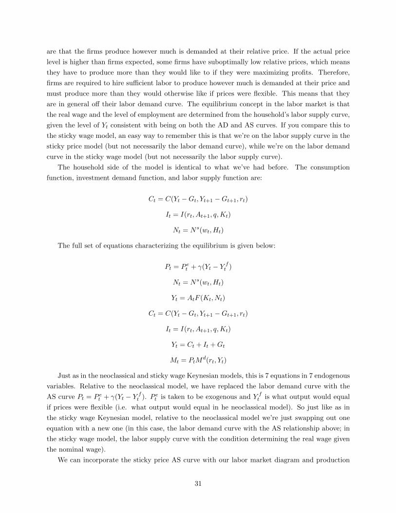
We can incorporate the sticky price AS curve with our labor market diagram and production

31

function in a way similar to what we have done before. If Pt = P et , the Yt = Y f

t and the labor

market equilibrium occurs where labor demand equals labor supply. If Pt < P et , however, then

Yt < Y ft . This means that Nt is smaller than would be the case at the intersection of the labor

demand and supply curves. In the sticky price model, we determine the quantity of labor and the

real wage off of the labor supply curve, not the labor demand curve. This means that if Pt < P et ,

then wt is smaller than what it would be if prices were flexible (and consequently labor hours are

smaller than they would be if prices were flexible). The reverse would be the case if Pt > P et . The

diagram below shows how things play out.

𝑌𝑌𝑡𝑡

𝑤𝑤𝑡𝑡

𝑌𝑌𝑡𝑡

𝑌𝑌𝑡𝑡

𝑌𝑌𝑡𝑡

𝑃𝑃𝑡𝑡



𝑁𝑁𝑠𝑠(𝑤𝑤𝑡𝑡,𝐻𝐻𝑡𝑡) 𝐴𝐴𝐴𝐴

𝑃𝑃𝑡𝑡1

𝑃𝑃𝑡𝑡𝑒𝑒 = 𝑃𝑃𝑡𝑡0

𝑁𝑁𝑑𝑑(𝑤𝑤𝑡𝑡,𝐴𝐴𝑡𝑡,𝐾𝐾𝑡𝑡)

𝑌𝑌𝑡𝑡0 = 𝑌𝑌𝑡𝑡𝑓𝑓 𝑌𝑌𝑡𝑡1

𝑤𝑤𝑡𝑡0 𝑤𝑤𝑡𝑡1

𝑁𝑁𝑡𝑡0 𝑁𝑁𝑡𝑡1

AS: 𝑃𝑃𝑡𝑡 = 𝑃𝑃𝑡𝑡𝑒𝑒 + 𝛾𝛾(𝑌𝑌𝑡𝑡 − 𝑌𝑌𝑡𝑡𝑓𝑓)

𝑁𝑁𝑡𝑡

𝑁𝑁𝑡𝑡

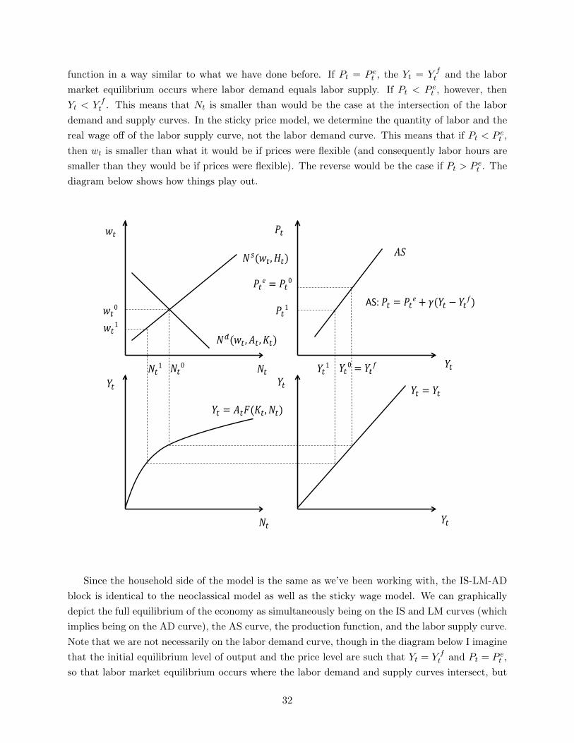
Since the household side of the model is the same as we’ve been working with, the IS-LM-AD

block is identical to the neoclassical model as well as the sticky wage model. We can graphically

depict the full equilibrium of the economy as simultaneously being on the IS and LM curves (which

implies being on the AD curve), the AS curve, the production function, and the labor supply curve.

Note that we are not necessarily on the labor demand curve, though in the diagram below I imagine

that the initial equilibrium level of output and the price level are such that Yt = Y ft and Pt = P e

t ,

so that labor market equilibrium occurs where the labor demand and supply curves intersect, but

32

in general this need not be the case. The picture below graphically characterizes the equilibrium.

𝐴𝐴𝐴𝐴

𝐿𝐿𝐿𝐿

𝐼𝐼𝐴𝐴

𝐴𝐴𝐴𝐴




𝑤𝑤𝑡𝑡


𝑤𝑤𝑡𝑡0

𝑌𝑌𝑡𝑡0 = 𝑌𝑌𝑡𝑡𝑓𝑓


𝑟𝑟𝑡𝑡0

𝑌𝑌𝑡𝑡

𝑌𝑌𝑡𝑡

𝑌𝑌𝑡𝑡



𝑁𝑁𝑡𝑡

𝑟𝑟𝑡𝑡

In terms of the equations given above, the IS curve again summarizes the consumption function,

the investment demand function, and the resource constraint. The LM curve summarizes the

condition that money demand equals money supply. The AS curve is the equation that is given.

We then determine the real wage and quantity of employment using the production function and

the labor supply curve.

33

In terms of the IS-LM-AD-AS curves, there is no qualitative difference between the sticky wage

and sticky price models. The differences in the models arise because of different assumptions about

why the AS curve isn’t perfectly vertical and what the notion of equilibrium in the labor market is.

In the sticky wage model, the nominal wage is fixed and the quantity of labor is read off the labor

demand curve at the Nt consistent with the value of Yt where the AD and AS curves intersect.

In the sticky price model, the price level is sticky and the quantity of labor is read off the labor

supply curve given the level of Nt consistent with the Yt where the AD and AS curves intersect.

In other words, if all you care about is the behavior of output, prices, and the interest rate, from

a qualitative perspective it does not matter whether the AS curve is not vertical because of sticky

prices or sticky wages. But for understanding what happens in the labor market, and understanding

optimal economic policy, the reason behind the upward-sloping AS curve will matter, as we will

learn later.

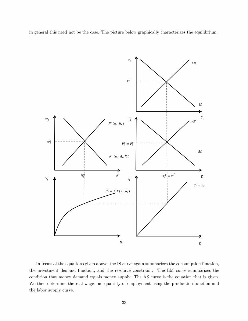
Now, let’s go through and analyze how the endogenous variables change in response to changes

in exogenous variables. Consider first an increase in the money supply. This shifts the LM curve

out (blue line), which in turn causes the AD curve to shift to the right (also a blue line). The

outward shift of the AD curve along an upward-sloping AS curve results in increases in both Yt

and Pt. The higher Pt causes the LM curve to shift back in some (green line), though not all the

way to where it started (unlike what would happen in the neoclassical model). This means that

the real interest rate is lower in the new equilibrium. Higher Yt and lower rt means that both Ct

and It are higher in the new equilibrium. Turning to the labor market, since Yt is higher it must

be the case that Nt is higher. Since we are determining labor from the labor supply curve (not the

labor demand curve), getting households to supply more labor requires a higher real wage.

34

𝐴𝐴𝐴𝐴


𝐼𝐼𝐴𝐴

𝐴𝐴𝐴𝐴




𝑤𝑤𝑡𝑡


𝑤𝑤𝑡𝑡0

𝑌𝑌𝑡𝑡0

𝑃𝑃𝑡𝑡0

𝑟𝑟𝑡𝑡0

𝑌𝑌𝑡𝑡

𝑌𝑌𝑡𝑡

𝑌𝑌𝑡𝑡



𝑁𝑁𝑡𝑡

𝑟𝑟𝑡𝑡

𝑌𝑌𝑡𝑡1

𝑟𝑟𝑡𝑡1

𝑃𝑃𝑡𝑡1

𝑁𝑁𝑡𝑡1




𝐴𝐴𝐴𝐴′

𝑤𝑤𝑡𝑡1

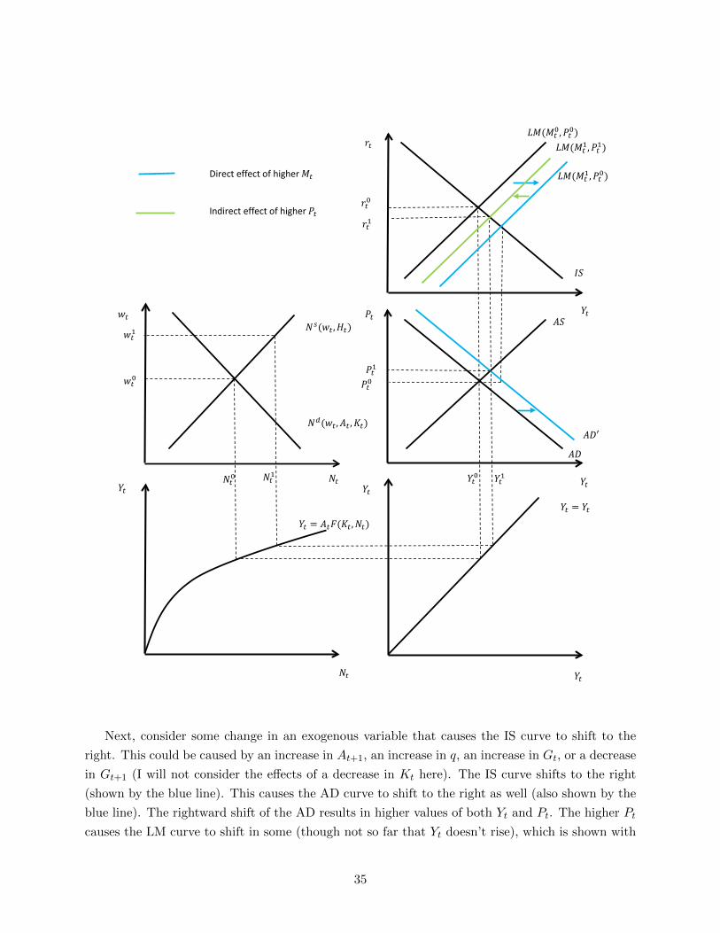
Next, consider some change in an exogenous variable that causes the IS curve to shift to the

right. This could be caused by an increase in At+1, an increase in q, an increase in Gt, or a decrease

in Gt+1 (I will not consider the effects of a decrease in Kt here). The IS curve shifts to the right

(shown by the blue line). This causes the AD curve to shift to the right as well (also shown by the

blue line). The rightward shift of the AD results in higher values of both Yt and Pt. The higher Pt

causes the LM curve to shift in some (though not so far that Yt doesn’t rise), which is shown with

35

the green line. The real interest rate is therefore higher in the new equilibrium. Since Yt is higher

but At is unchanged, Nt must be higher. Since we determine labor from the labor supply curve, it

must be the case that wt is higher to induce households to work more.

𝐴𝐴𝐴𝐴


𝐼𝐼𝐴𝐴

𝐴𝐴𝐴𝐴




𝑤𝑤𝑡𝑡


𝑤𝑤𝑡𝑡0

𝑌𝑌𝑡𝑡0

𝑃𝑃𝑡𝑡0

𝑟𝑟𝑡𝑡0

𝑌𝑌𝑡𝑡

𝑌𝑌𝑡𝑡

𝑌𝑌𝑡𝑡



𝑁𝑁𝑡𝑡

𝑟𝑟𝑡𝑡

𝑌𝑌𝑡𝑡1

𝑟𝑟𝑡𝑡1

𝑃𝑃𝑡𝑡1

𝑁𝑁𝑡𝑡1



𝐼𝐼𝐴𝐴′

𝑤𝑤𝑡𝑡1

𝐴𝐴𝐴𝐴′

How consumption and investment are affected depends on the exogenous variable which is

changing. These effects are going to be qualitatively similar to what we saw in the sticky wage

model. When At+1 increases, the effects on both Ct and It are ambiguous, though we know that

36

at least one of them must increase (and they may both increase, in spite of the higher real interest

rate). When q increases, we know that It increases (in spite of the increase in the real interest rate,

since It would increase in the neoclassical model, and the real interest rate increases less here). We

cannot determine whether Ct increases or decreases. When Gt increases, we know that both Ct

and It must decrease. The decrease in It is clear from the increase in rt. The reason why we know

that Ct decreases is that Yt increases by less than Gt, so that Yt −Gt declines. Combined with rt

increasing, we therefore know that Ct must fall. When Gt+1 falls, we know that It falls because rt

is higher. Since Yt is higher but Gt is not affected, we can deduce that Ct must increase.

Consider next the effects of an increase in At. This causes the AS curve to shift horizontally to

the right. The magnitude of the horizontal shift is equal to the change in Y ft , which can graphically

be determined as the level of Yt that would obtain if we were on both the new labor demand and

supply curves as well as the new production function. As long as the AS curve is not vertical (and

the AD curve not completely horizontal), we see that Yt will increase and Pt will fall. Graphically,

the increase in Yt is smaller than the horizontal shift of the AS curve – put another way, Yt increases

by less than it would if prices were flexible. The lower price level causes the LM curve to shift right,

so that the real interest rate is lower. A lower real interest rate plus higher output means that both

Ct and It are higher in the new equilibrium. Turning to the labor market, the level of employment

must be consistent with the level of Yt where the AD and AS curves intersect. The equilibrium

real wage is then read off the labor supply curve at this level of Nt. As drawn here, we actually

get a decline in the real wage and a decline in Nt. These effects are technically ambiguous (in a

way similar to how the effects of a productivity shock on labor hours were ambiguous in the sticky

wage model). The real wage and labor hours could rise, and it would be more likely that they do

if the AD curve is very flat (or the AS curve very steep). We will return to this point below.

37

𝐴𝐴𝐴𝐴


𝐼𝐼𝐴𝐴

𝐴𝐴𝐴𝐴




𝑤𝑤𝑡𝑡


𝑤𝑤𝑡𝑡0



𝑟𝑟𝑡𝑡0

𝑌𝑌𝑡𝑡

𝑌𝑌𝑡𝑡

𝑌𝑌𝑡𝑡



𝑁𝑁𝑡𝑡

𝑟𝑟𝑡𝑡



𝐴𝐴𝐴𝐴′


𝑤𝑤𝑡𝑡1 𝑃𝑃𝑡𝑡1

𝑌𝑌𝑡𝑡𝑓𝑓′ 𝑌𝑌𝑡𝑡1 𝑁𝑁𝑡𝑡1


𝑟𝑟𝑡𝑡1

𝑌𝑌𝑡𝑡𝑓𝑓′: what the level of output

would be with higher 𝐴𝐴𝑡𝑡 if prices were flexible

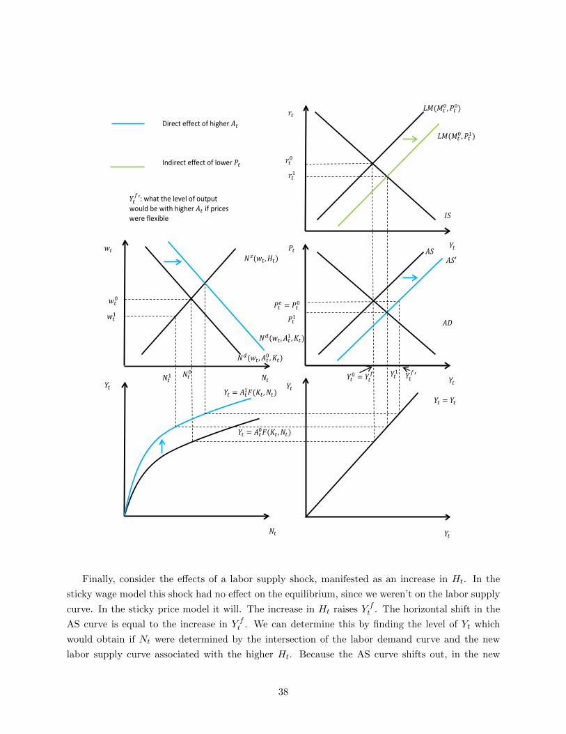
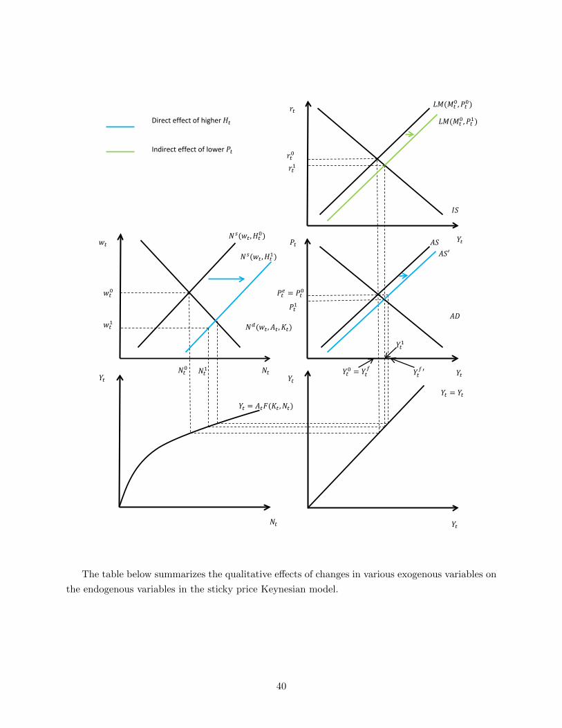
Finally, consider the effects of a labor supply shock, manifested as an increase in Ht. In the

sticky wage model this shock had no effect on the equilibrium, since we weren’t on the labor supply

curve. In the sticky price model it will. The increase in Ht raises Y ft . The horizontal shift in the

AS curve is equal to the increase in Y ft . We can determine this by finding the level of Yt which

would obtain if Nt were determined by the intersection of the labor demand curve and the new

labor supply curve associated with the higher Ht. Because the AS curve shifts out, in the new

38

equilibrium Yt is higher and Pt is lower. That being said, unless the AS curve is vertical (or the AD

curve perfectly horizontal), the increase in Yt is smaller than the increase in Y ft (i.e. the increase

in Yt is smaller than the horizontal shift of the AS curve, in a way similar to what we saw for the

case of an increase in At above). The lower price level causes the LM curve to shift to the right,

which results in a lower real interest rate. A lower real interest rate plus higher output means that

both Ct and It are higher in the new equilibrium. Turning back to the labor market, the new level

of Nt must be consistent with the Yt where the AD and AS curves intersect. This is smaller than

the new Nt would be if prices were flexible (e.g. the AS were vertical). We determine the real wage

off of the new labor supply curve at the new equilibrium level of Nt. We see that wt is smaller in

the new equilibrium.

39

𝐴𝐴𝐴𝐴


𝐼𝐼𝐴𝐴

𝐴𝐴𝐴𝐴




𝑤𝑤𝑡𝑡




𝑟𝑟𝑡𝑡0

𝑌𝑌𝑡𝑡

𝑌𝑌𝑡𝑡

𝑌𝑌𝑡𝑡



𝑁𝑁𝑡𝑡

𝑟𝑟𝑡𝑡


𝐴𝐴𝐴𝐴′

𝑌𝑌𝑡𝑡𝑓𝑓′

𝑌𝑌𝑡𝑡1

𝑁𝑁𝑡𝑡1

𝑤𝑤𝑡𝑡0

𝑤𝑤𝑡𝑡1

𝑟𝑟𝑡𝑡1

𝑃𝑃𝑡𝑡1

Direct effect of higher 𝐻𝐻𝑡𝑡 Indirect effect of lower 𝑃𝑃𝑡𝑡


The table below summarizes the qualitative effects of changes in various exogenous variables on

the endogenous variables in the sticky price Keynesian model.

40

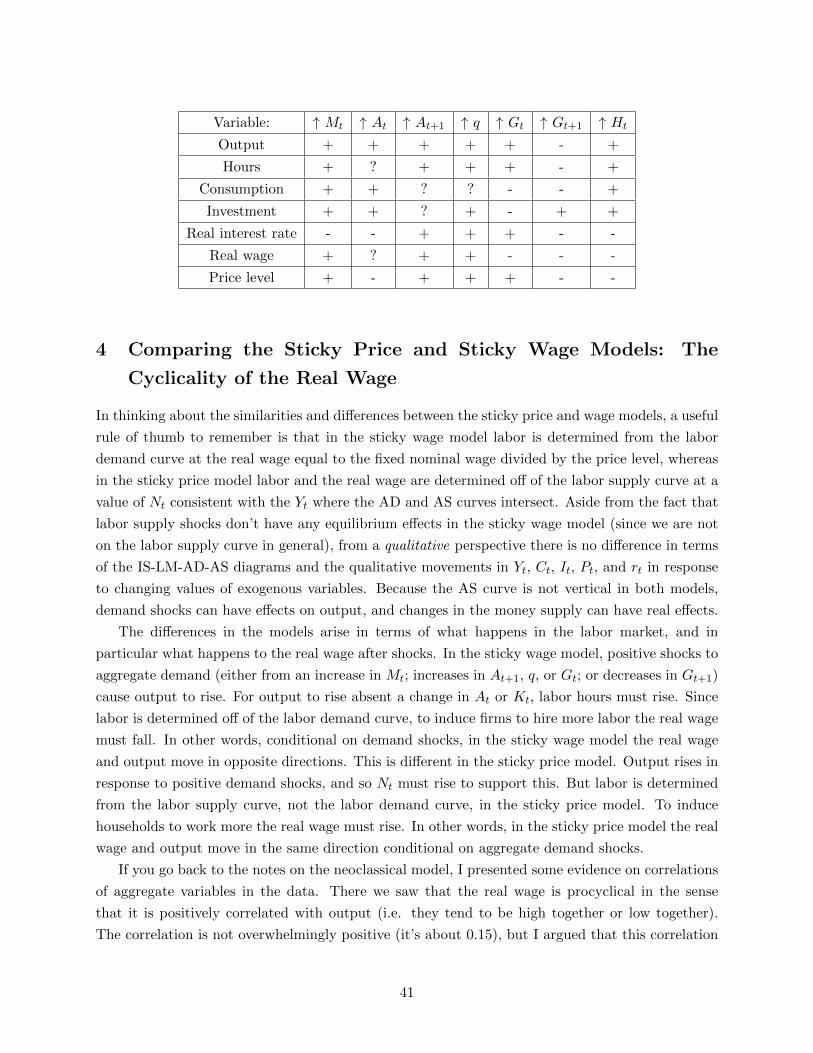
Variable: ↑ Mt ↑ At ↑ At+1 ↑ q ↑ Gt ↑ Gt+1 ↑ Ht

Output + + + + + - +

Hours + ? + + + - +

Consumption + + ? ? - - +

Investment + + ? + - + +

Real interest rate - - + + + - -

Real wage + ? + + - - -

Price level + - + + + - -

4 Comparing the Sticky Price and Sticky Wage Models: The

Cyclicality of the Real Wage

In thinking about the similarities and differences between the sticky price and wage models, a useful

rule of thumb to remember is that in the sticky wage model labor is determined from the labor

demand curve at the real wage equal to the fixed nominal wage divided by the price level, whereas

in the sticky price model labor and the real wage are determined off of the labor supply curve at a

value of Nt consistent with the Yt where the AD and AS curves intersect. Aside from the fact that

labor supply shocks don’t have any equilibrium effects in the sticky wage model (since we are not

on the labor supply curve in general), from a qualitative perspective there is no difference in terms

of the IS-LM-AD-AS diagrams and the qualitative movements in Yt, Ct, It, Pt, and rt in response

to changing values of exogenous variables. Because the AS curve is not vertical in both models,

demand shocks can have effects on output, and changes in the money supply can have real effects.

The differences in the models arise in terms of what happens in the labor market, and in

particular what happens to the real wage after shocks. In the sticky wage model, positive shocks to

aggregate demand (either from an increase in Mt; increases in At+1, q, or Gt; or decreases in Gt+1)

cause output to rise. For output to rise absent a change in At or Kt, labor hours must rise. Since

labor is determined off of the labor demand curve, to induce firms to hire more labor the real wage

must fall. In other words, conditional on demand shocks, in the sticky wage model the real wage

and output move in opposite directions. This is different in the sticky price model. Output rises in

response to positive demand shocks, and so Nt must rise to support this. But labor is determined

from the labor supply curve, not the labor demand curve, in the sticky price model. To induce

households to work more the real wage must rise. In other words, in the sticky price model the real

wage and output move in the same direction conditional on aggregate demand shocks.

If you go back to the notes on the neoclassical model, I presented some evidence on correlations

of aggregate variables in the data. There we saw that the real wage is procyclical in the sense

that it is positively correlated with output (i.e. they tend to be high together or low together).

The correlation is not overwhelmingly positive (it’s about 0.15), but I argued that this correlation

41

probably understates the actual procyclicality of the real wage because of things like the composition

bias. If you take as given that the real wage is procyclical, does this provide any insight into which

variant of the Keynesian model might better fit the data? To the extent to which you think

aggregate demand shocks are an important driver of output, it does. Since the sticky price model

predicts a positive correlation between real wages and output conditional on demand shocks, this

would seemingly be a better-fitting model than the sticky wage model. It’s largely for this reason

that the class of “New Keynesian” models developed in academia in the 1980s and 1990s emphasize

price stickiness as the key nominal rigidity, not wage stickiness. More modern variants of the model

used at the frontiers of academic research often feature both wage and price stickiness, but a model

with sticky wages alone will not do a good job of producing a procyclical real wage conditional on

demand shocks.

5 Supply Shocks in the Keynesian Model

Loosely speaking, we can think about there being two kinds of shocks (“shocks” = change in an

exogenous variable) that affect output: supply shocks (things which shift the AS curve) and demand

shocks (things which shift the AD curve). In the neoclassical model the AS curve is vertical, which

means that demand shocks cannot affect output. One key difference between the Keynesian and

neoclassical models is that both variants of the Keynesian model feature a non-vertical AS curve,

which allows output to react to demand shocks.

As we saw above, supply shocks can and do affect output in the Keynesian model. For the rest

of this section, let’s focus on a change in productivity, At, as the supply shock (since changes in Ht

don’t affect the AS curve in the sticky wage model). Whereas in the neoclassical model an increase

in At causes Nt to rise, in both variants of the Keynesian model the effect on Nt is ambiguous (in

the graphs above I showed Nt as not changing after an increase in At in the sticky wage model and

as falling after an increase in At in the sticky price model). I want to explore this point about the

ambiguous effect of a change in At on Nt in the Keynesian model a little more carefully here.

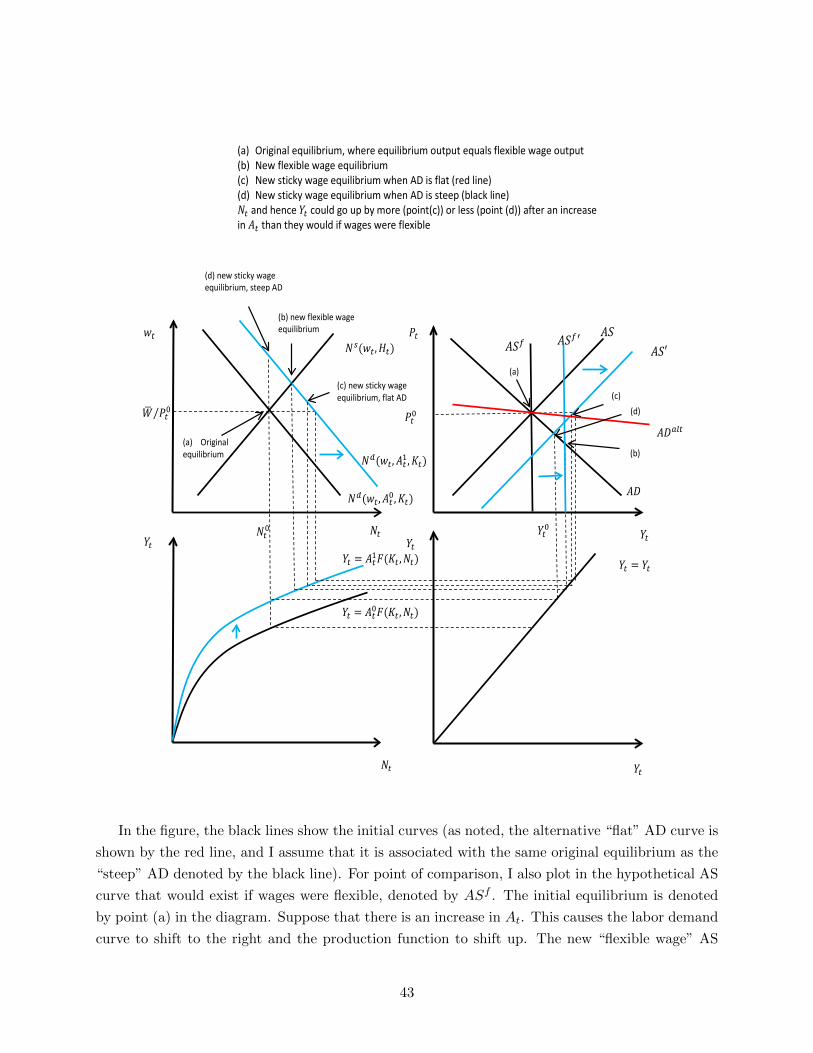
Let’s begin with the sticky wage Keynesian model. I want to consider the effects of an increase

in At on Nt (and other variables) in that model. To make the point as clear as possible, I’m going

to do so with two AD curves. One is relatively steep (black line) while the other is relatively flat

(red line). The effects of an increase in At are shown in the following diagram, which is explained

in more detail below. For ease of exposition, I omit the IS-LM diagram here.

42

𝐴𝐴𝐴𝐴




𝑤𝑤𝑡𝑡



𝑌𝑌𝑡𝑡0

𝑃𝑃𝑡𝑡0

𝑌𝑌𝑡𝑡

𝑌𝑌𝑡𝑡

𝑌𝑌𝑡𝑡


𝑃𝑃𝑡𝑡

𝑁𝑁𝑡𝑡

𝐴𝐴𝐴𝐴𝑎𝑎𝑎𝑎𝑡𝑡



(a) Original equilibrium

(b) new flexible wage equilibrium

(d) new sticky wage equilibrium, steep AD

(c) new sticky wage equilibrium, flat AD

(a)

(b)

(c) (d)

𝐴𝐴𝐴𝐴𝑓𝑓 𝐴𝐴𝐴𝐴𝑓𝑓′ 𝐴𝐴𝐴𝐴 𝐴𝐴𝐴𝐴′

(a) Original equilibrium, where equilibrium output equals flexible wage output (b) New flexible wage equilibrium (c) New sticky wage equilibrium when AD is flat (red line) (d) New sticky wage equilibrium when AD is steep (black line) 𝑁𝑁𝑡𝑡 and hence 𝑌𝑌𝑡𝑡 could go up by more (point(c)) or less (point (d)) after an increase in 𝐴𝐴𝑡𝑡 than they would if wages were flexible

In the figure, the black lines show the initial curves (as noted, the alternative “flat” AD curve is

shown by the red line, and I assume that it is associated with the same original equilibrium as the

“steep” AD denoted by the black line). For point of comparison, I also plot in the hypothetical AS

curve that would exist if wages were flexible, denoted by ASf . The initial equilibrium is denoted

by point (a) in the diagram. Suppose that there is an increase in At. This causes the labor demand

curve to shift to the right and the production function to shift up. The new “flexible wage” AS

43

curve, ASf ′ (shown in blue) can be determined as the level of Yt consistent with the intersection of

the new labor demand curve and the labor supply curve and with the production function. Hence,

ASf shifts to the right, just as it would in the neoclassical model using these graphs. We determine

the new level of Yt if wages were flexible where the new vertical ASf curve intersects the AD curve,

labeled (b) in the diagram.

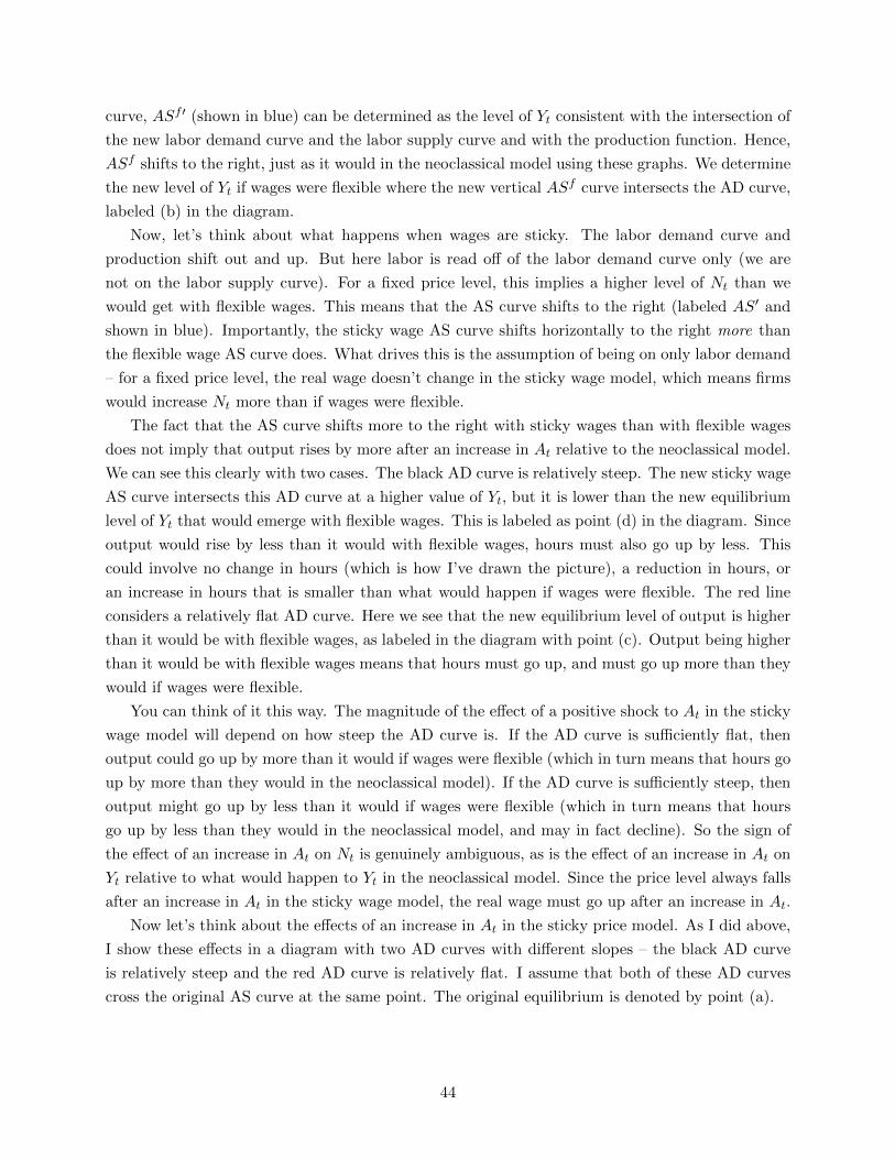
Now, let’s think about what happens when wages are sticky. The labor demand curve and

production shift out and up. But here labor is read off of the labor demand curve only (we are

not on the labor supply curve). For a fixed price level, this implies a higher level of Nt than we

would get with flexible wages. This means that the AS curve shifts to the right (labeled AS′ and

shown in blue). Importantly, the sticky wage AS curve shifts horizontally to the right more than

the flexible wage AS curve does. What drives this is the assumption of being on only labor demand

– for a fixed price level, the real wage doesn’t change in the sticky wage model, which means firms

would increase Nt more than if wages were flexible.

The fact that the AS curve shifts more to the right with sticky wages than with flexible wages

does not imply that output rises by more after an increase in At relative to the neoclassical model.

We can see this clearly with two cases. The black AD curve is relatively steep. The new sticky wage

AS curve intersects this AD curve at a higher value of Yt, but it is lower than the new equilibrium

level of Yt that would emerge with flexible wages. This is labeled as point (d) in the diagram. Since

output would rise by less than it would with flexible wages, hours must also go up by less. This

could involve no change in hours (which is how I’ve drawn the picture), a reduction in hours, or

an increase in hours that is smaller than what would happen if wages were flexible. The red line

considers a relatively flat AD curve. Here we see that the new equilibrium level of output is higher

than it would be with flexible wages, as labeled in the diagram with point (c). Output being higher

than it would be with flexible wages means that hours must go up, and must go up more than they

would if wages were flexible.

You can think of it this way. The magnitude of the effect of a positive shock to At in the sticky

wage model will depend on how steep the AD curve is. If the AD curve is sufficiently flat, then

output could go up by more than it would if wages were flexible (which in turn means that hours go

up by more than they would in the neoclassical model). If the AD curve is sufficiently steep, then

output might go up by less than it would if wages were flexible (which in turn means that hours

go up by less than they would in the neoclassical model, and may in fact decline). So the sign of

the effect of an increase in At on Nt is genuinely ambiguous, as is the effect of an increase in At on

Yt relative to what would happen to Yt in the neoclassical model. Since the price level always falls

after an increase in At in the sticky wage model, the real wage must go up after an increase in At.

Now let’s think about the effects of an increase in At in the sticky price model. As I did above,

I show these effects in a diagram with two AD curves with different slopes – the black AD curve

is relatively steep and the red AD curve is relatively flat. I assume that both of these AD curves

cross the original AS curve at the same point. The original equilibrium is denoted by point (a).

44

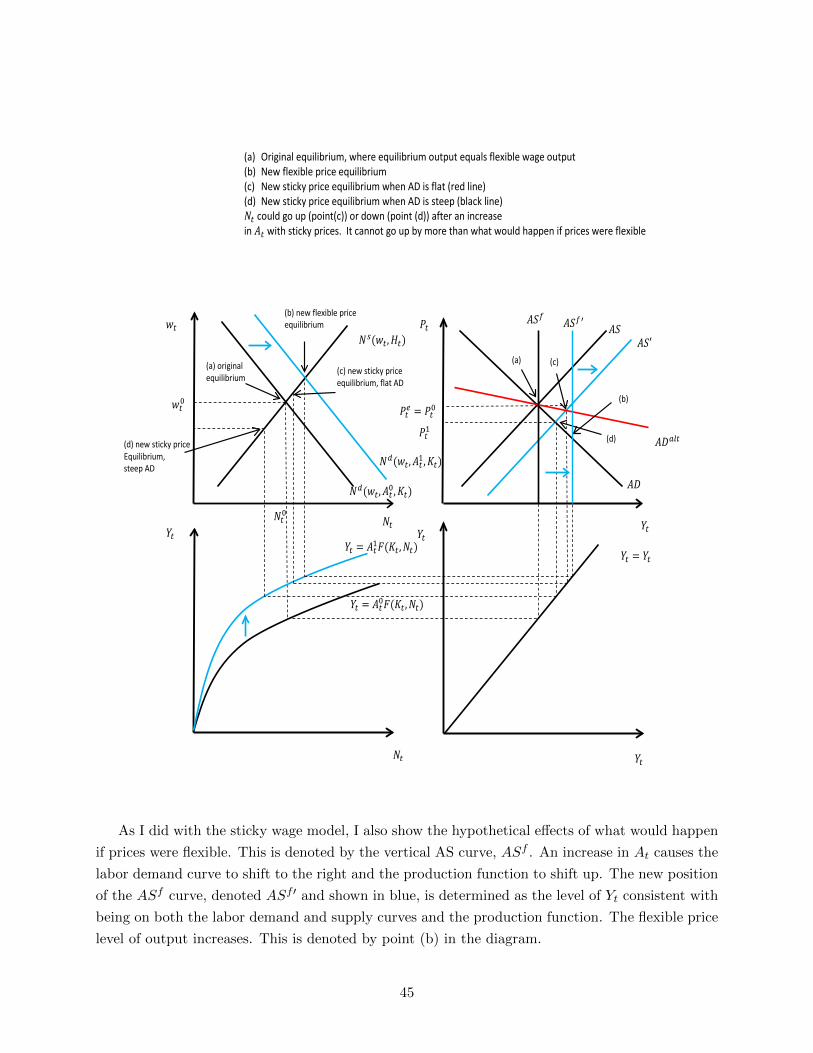
𝐴𝐴𝐴𝐴

𝐴𝐴𝐴𝐴




𝑤𝑤𝑡𝑡


𝑤𝑤𝑡𝑡0 𝑃𝑃𝑡𝑡𝑒𝑒 = 𝑃𝑃𝑡𝑡0

𝑌𝑌𝑡𝑡

𝑌𝑌𝑡𝑡

𝑌𝑌𝑡𝑡


𝑃𝑃𝑡𝑡

𝑁𝑁𝑡𝑡



𝐴𝐴𝐴𝐴′

𝑃𝑃𝑡𝑡1 𝐴𝐴𝐴𝐴𝑎𝑎𝑎𝑎𝑡𝑡

(a) original equilibrium

(b) new flexible price equilibrium

(c) new sticky price equilibrium, flat AD

(d) new sticky price Equilibrium, steep AD

𝐴𝐴𝐴𝐴𝑓𝑓 𝐴𝐴𝐴𝐴𝑓𝑓′

(a)

(b)

(d)

(c)

(a) Original equilibrium, where equilibrium output equals flexible wage output (b) New flexible price equilibrium (c) New sticky price equilibrium when AD is flat (red line) (d) New sticky price equilibrium when AD is steep (black line) 𝑁𝑁𝑡𝑡 could go up (point(c)) or down (point (d)) after an increase in 𝐴𝐴𝑡𝑡 with sticky prices. It cannot go up by more than what would happen if prices were flexible

As I did with the sticky wage model, I also show the hypothetical effects of what would happen

if prices were flexible. This is denoted by the vertical AS curve, ASf . An increase in At causes the

labor demand curve to shift to the right and the production function to shift up. The new position

of the ASf curve, denoted ASf ′ and shown in blue, is determined as the level of Yt consistent with

being on both the labor demand and supply curves and the production function. The flexible price

level of output increases. This is denoted by point (b) in the diagram.

45

Now, let’s consider what would happen with sticky prices. The AS curve would shift horizontally

to the right by the change in Y ft . In other words, the horizontal shift of the AS curve in the sticky

price model is the same as the horizontal shift of the hypothetical AS curve if prices were flexible.

But because the AS curve in the sticky price model is not vertical, the change in equilibrium Yt

in the sticky price model is always smaller than it would be if prices were flexible. This is true

whether the AD curve is relatively flat (red AD curve, new equilibrium denoted by point (c)) or

relatively steep (black line, new equilibrium denoted by point (d)). Since output necessarily goes up

by less in the sticky price model relative to the flexible price model, the increase in Nt is necessarily

smaller than it would be if prices were flexible. It is true that the flatter is the AD curve, the more

output increases in the sticky price model after an increase in At, but it cannot go up by more

than it does in the flexible price model. If the AD curve is relatively flat, then output goes up by

relatively a lot, which means it is likely that Nt increases in the sticky price model (and that the

real wage increases). But if the AD curve is relatively steep, then it is possible that Nt declines

(and hence so too does wt). Hence, the effect of an increase in At on Nt (and wt) in the sticky

price model is ambiguous. Whether Nt (and wt) go up or down depends on the steepness of the

AD curve. In any event, Nt (and wt) will increase by less in the sticky price model than it would

in the flexible price neoclassical model.

In both the sticky price and wage models, it is conceivable that Nt declines after a productivity

improvement (increase in Nt). Is there any empirical evidence to support this? It turns out there

is. A number of papers seek to empirically identify surprise changes in At and assess their impact

on endogenous variables like Nt. Many of these papers find that Nt declines when productivity

improves, a finding which is inconsistent with the neoclassical model but potentially consistent

with the Keynesian model (either the sticky wage or sticky price version). Gali (1999) uses a

restriction that only productivity changes can impact output in the “long run” and finds that

productivity improvements are associated with reductions in hours worked.5 Basu, Fernald, and

Kimball (2006) construct a “purified” measure of total factor productivity (TFP) meant to proxy

for the model-based At. The “purification” refers to the fact that they try to control for unobserved

input variation, which they argue is important and contaminates traditional measures of TFP like

the one I produced in the neoclassical model notes.6 They find that improvements in their purified

TFP measure are also associated with declines in total hours worked.7 Both Gali (1999) and Basu,

Fernald, and Kimball (2006) argue that this is strong evidence against the neoclassical model and

points towards Keynesian theories. There does exist some countervailing evidence that argues that

5Gali, Jordi. 1999. “Technology, Employment, and the Business Cycle: Do Technology Shocks Explain AggregateFluctuations?” American Economic Review 89(1): 249-271.

6The basic idea of unobserved input variation is that measured Kt and Nt may be poor measures of true capitaland labor input. Suppose that we are in a Keynesian model and output goes up due to a positive demand shock.Firms may work their capital and machines “harder” in such a way that actual Kt and Nt rise by more than what wecan observe in the data. This would mechanically make it look like At is increasing, even though it’s really not. These(and other) authors argue that unobserved input variation is primarily responsible for the strong positive correlationbetween measured TFP and output that we saw in the last set of notes, not actual changes in productivity occurringat the same time as fluctuations in output.

7Basu, Susanto, John Fernald, and Miles S. Kimball. 2006. “Are Technology Improvements Contractionary?”American Economic Review 96(5): 1418-1448.

46

hours increase after improvements in At in a way consistent with the implications of the neoclassical

model.

When comparing the Keynesian model to the neoclassical model, there are some nice di-

chotomies that are easy to remember. In the neoclassical model, only supply shocks (changes

in At or Ht) can affect output. In the Keynesian model (either the sticky price or sticky wage

version), demand shocks can matter too. In the sticky price model, supply shocks (changes in

either At or Ht) have smaller effects on Yt and other real variables relative to a neoclassical model.

In the sticky wage model, labor supply shocks have no effect on real variables, and these effects

are therefore smaller than they would be if wages were flexible. The effects of changes in At on

Yt in the sticky wage model may be smaller or larger than in the neoclassical model depending

on the slope of the AD curve. To make things easy to remember, we will hereafter assume that

the AD curve is sufficiently steep so that output rises by less after an increase in At in the sticky

wage Keynesian model than it would in the neoclassical model. This means that we can draw the

following conclusion: relative to the neoclassical model, demand shocks have bigger real effects and

supply shocks smaller real effects in the Keynesian model (either the sticky price or sticky wage

version).

6 Sticky Prices and Wages: Empirical Evidence

Relative to the neoclassical model, the key friction in Keynesian theories is nominal rigidity – prices

and/or wages are imperfectly flexible. This imperfect flexibility allows demand shocks to have real

effects and changes the way that supply shocks impact the real side of the economy. As we will

see, Keynesian theories also have different normative implications for economic policy than does

the neoclassical model, where there is no justification for activist policies.

If we want to take Keynesian theories seriously, we would like to get a sense of whether or not

there is any empirical evidence to support price and/or wage stickiness. It turns out that there has

been a decent amount of research into this area. Bils and Klenow (2004) is a comprehensive study

that makes use of unpublished data on prices of over 350 categories of goods.8 They find evidence

that prices are sticky – the median duration between prices changes across all varieties of goods is

roughly six months, or two quarters. This is broadly consistent with the notion that at least some

prices do not react instantaneously to changing aggregate conditions as in our simple sticky price

model. There is great heterogeneity in frequency of price duration across different varieties of goods

– some goods have prices which change daily (e.g. gasoline), while there are other goods whose

prices change on average only every couple of years (e.g. newspapers). While there is thus some

good evidence that prices are sticky, some neoclassical economists have countered that the observed

level of stickiness is not sufficiently long for price stickiness to be important over the medium term

(frequencies of 1-3 years).

There is also evidence on the importance of wage rigidity. Barattieri, Basu, and Gottschalk

8Bils, Mark and Peter Klenow. 2004. “Some Evidence on the Importance of Sticky Prices.” Journal of PoliticalEconomy 112(5): 947-985.

47

(2014) argue that nominal wages adjust on average only once a year or so, which in terms of

duration between changes is significantly longer than for prices.9 This is also broadly consistent

with the sticky wage model. There are some potential issues here. In particular, what may be

macroeconomically relevant is wage rigidity for new hires, not wages of existing hires. There is

some evidence that new hire wages adjust quite a lot and rather frequently.

Nevertheless, given all this evidence, as well as the empirical evidence that demand shocks

matter, most modern macroeconomic models incorporate at sticky prices or sticky wages, and

often use both at the same time. In that sense, some version of the Keynesian model (a little more

sophisticated than what we’ve done here, but I’ve provided you with the basic gist) has more or

less become the “standard” model that academic macroeconomists and central bankers use. As I

stated at the beginning, it’s important to emphasize that we shouldn’t think of this model as wholly

different from the neoclassical model. Rather, the neoclassical model can be thought of as a special

case of a Keynesian model in which there is no nominal rigidity. In that sense, the neoclassical

model is a building block of Keynesian models and it is useful to understand that model well, even

if you don’t necessarily take its implications all that seriously.

7 Dynamics: From Short Run to Medium Run

Price and/or wage stickiness are fundamentally “short run” phenomena. By that I mean that

while there may be frictions that prevent the instantaneous adjustment of prices and/or wages to

changing aggregate conditions, eventually prices and wages should be able to adjust. This is also

consistent with the empirical evidence – while there is some good evidence that prices and wages

are in fact sticky, they’re not sticky forever.

We want to briefly discuss how the economy ought to “dynamically” adjust to being away from

its flexible price/wage level. I put “dynamically” in quotes because we’re not doing dynamics in

the way we did in the Solow model. Here we only have two periods, and I don’t even want to

think about adjustments across periods (we really just have the t + 1 in there to motivate that

what happens today depends on what people think will happen in the future). But I do want to

think about forces that will be at work if the economy finds itself in an equilibrium that does not

correspond with what the equilibrium would be if prices and wages were flexible. The basic gist

is going to be this. If the economy finds itself at an equilibrium where Yt 6= Y ft (where Y f

t is the

level of output that would obtain if prices and/or wages were fully flexible), then the AS curve is

going to shift in such a way as to force the equilibrium to move towards Y ft . This will be true in

both the sticky wage and sticky price models. When thinking about these features, I’m going to

imagine this shift of the AS curve occurring within period t. We can take a liberal notion of how

long t is – if you like, think about a period as lasting 3-4 years. The economy may find itself in

an equilibrium away from Y ft for 1-2 years (think about this as the “short run”), but then in years

3-4 and the AS will shift to make the equilibrium correspond with Y ft (think about this as the

9Barattieri, Alessandro, Susanto Basu, and Peter Gottschalk. 2014. “Some Evidence on the Importance of StickyWages.” American Economic Journal: Macroeconomics 6(1): 70-101.

48

“medium run”). The “long run” corresponds to frequencies like decades, which we thought about

in the Solow Model.

Let’s first start with the sticky wage version of the Keynesian model. Suppose that the economy

initially sits in an equilibrium in which Y 0t < Y f

t . Y ft is the level of output that would obtain if we

were at the intersection of the labor demand and supply curves. This is denoted by point (b) in the

graph below. The actual equilibrium is denoted by point (a). If output is below its flexible wage

level, this means that Nt is lower than it would be if wages were flexible. Because we are always

on the labor demand curve in the sticky wage model, this must mean that the real wage is higher

than it would be with flexible wages.

Now, let’s think about the incentives that actors in the economy face should the economy find

itself in a position like this. For output to be below its flexible wage level, the real wage is higher

than is optimal. In terms of the figure, there is an excess supply of labor at the initial real wage

– the quantity of labor supplied (which is not what is relevant for output, since we are not on

the labor supply curve) exceeds the quantity of labor demanded at this wage. This means that

there ought to be downward pressure on the nominal wage – an excess supply of something ought

to drive down the price of that thing (in this case, the wage). In other words, we would expect

that, over time as it is able to adjust, the nominal wage ought to adjust downward. A downward

adjustment in the nominal wage would work to shift the AS curve to the right – a downward change

in W represents a movement down the labor demand curve for a given price level, resulting in more

employment and hence more output for each price level, i.e. an outward shift of the AS curve. Over

time, the nominal wage will adjust to some new level, call it W′, in such a way that the AS curve

will shift so as to intersect the AD curve at Y ft . In other words, we would expect the nominal wage

to adjust in such a way as to shift the AS curve to “close the gap” in the sense of eliminating any

difference between equilibrium output and its flexible wage level. The new sticky wage equilibrium

in the “medium run” (point (c)) ought to converge to the flexible wage equilibrium. The outward

shift of the AS curve (shown with the purple line) results in a fall in the price level. Something

similar would happen (but in reverse) if we happened to find ourselves in an initial equilibrium in

which Yt > Y ft : the nominal wage would eventually adjust up, the AS curve would shift in so as to

“close the gap,” and the price level would rise.

49

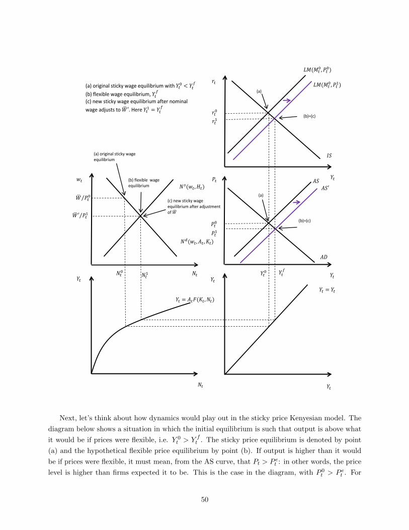
𝐴𝐴𝐴𝐴


𝐼𝐼𝐴𝐴

𝐴𝐴𝐴𝐴




𝑤𝑤𝑡𝑡



𝑌𝑌𝑡𝑡0

𝑃𝑃𝑡𝑡0

𝑟𝑟𝑡𝑡0

𝑌𝑌𝑡𝑡

𝑌𝑌𝑡𝑡

𝑌𝑌𝑡𝑡



𝑁𝑁𝑡𝑡

𝑟𝑟𝑡𝑡

𝑌𝑌𝑡𝑡𝑓𝑓

𝑃𝑃𝑡𝑡1


𝑊𝑊� ′ 𝑃𝑃𝑡𝑡1⁄

𝐴𝐴𝐴𝐴′

𝑟𝑟𝑡𝑡1

(a) original sticky wage equilibrium

(b) flexible wage equilibrium

(c) new sticky wage equilibrium after adjustment of 𝑊𝑊�

(a)

(b)=(c)

(a)

(b)=(c)

𝑁𝑁𝑡𝑡1

(a) original sticky wage equilibrium with 𝑌𝑌𝑡𝑡0 < 𝑌𝑌𝑡𝑡𝑓𝑓

(b) flexible wage equilibrium, 𝑌𝑌𝑡𝑡𝑓𝑓

(c) new sticky wage equilibrium after nominal wage adjusts to 𝑊𝑊� ′. Here 𝑌𝑌𝑡𝑡1 = 𝑌𝑌𝑡𝑡

𝑓𝑓

Next, let’s think about how dynamics would play out in the sticky price Kenyesian model. The

diagram below shows a situation in which the initial equilibrium is such that output is above what

it would be if prices were flexible, i.e. Y 0t > Y f

t . The sticky price equilibrium is denoted by point

(a) and the hypothetical flexible price equilibrium by point (b). If output is higher than it would

be if prices were flexible, it must mean, from the AS curve, that Pt > P et : in other words, the price

level is higher than firms expected it to be. This is the case in the diagram, with P 0t > P e

t . For

50

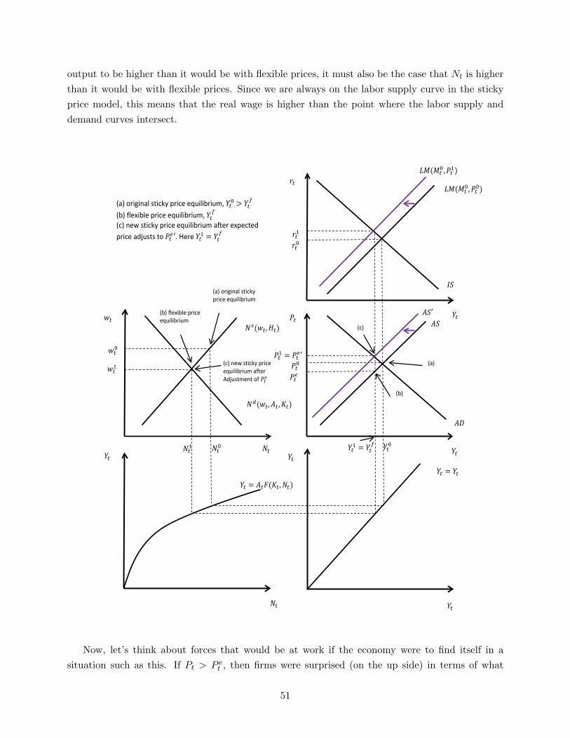
output to be higher than it would be with flexible prices, it must also be the case that Nt is higher

than it would be with flexible prices. Since we are always on the labor supply curve in the sticky

price model, this means that the real wage is higher than the point where the labor supply and

demand curves intersect.

𝐴𝐴𝐴𝐴


𝐼𝐼𝐴𝐴

𝐴𝐴𝐴𝐴




𝑤𝑤𝑡𝑡


𝑤𝑤𝑡𝑡0

𝑌𝑌𝑡𝑡0

𝑃𝑃𝑡𝑡𝑒𝑒

𝑟𝑟𝑡𝑡0

𝑌𝑌𝑡𝑡

𝑌𝑌𝑡𝑡

𝑌𝑌𝑡𝑡



𝑁𝑁𝑡𝑡

𝑟𝑟𝑡𝑡

𝑃𝑃𝑡𝑡0


𝑤𝑤𝑡𝑡1

𝑁𝑁𝑡𝑡1

𝐴𝐴𝐴𝐴′

𝑟𝑟𝑡𝑡1


𝑃𝑃𝑡𝑡1 = 𝑃𝑃𝑡𝑡𝑒𝑒′

(a) original sticky price equilibrium

(b) flexible price equilibrium

(c) new sticky price equilibrium after Adjustment of 𝑃𝑃𝑡𝑡𝑒𝑒

(a)

(b)

(c)

(a) original sticky price equilibrium, 𝑌𝑌𝑡𝑡0 > 𝑌𝑌𝑡𝑡𝑓𝑓

(b) flexible price equilibrium, 𝑌𝑌𝑡𝑡𝑓𝑓

(c) new sticky price equilibrium after expected price adjusts to 𝑃𝑃𝑡𝑡𝑒𝑒′. Here 𝑌𝑌𝑡𝑡1 = 𝑌𝑌𝑡𝑡

𝑓𝑓

Now, let’s think about forces that would be at work if the economy were to find itself in a

situation such as this. If Pt > P et , then firms were surprised (on the up side) in terms of what

51

they expected prices to be. Fool me once, shame on you. Fool me twice, shame on me. Firms

that were surprised will eventually update their expectations of the price level to conform with

reality. In other words, P et will increase over the medium run to something like P e′

t . An increase

in the expected price level works to shift the AS curve to the left (or up, if you prefer). This

is shown by the purple line in the graph. This will happen until the AS curve shifts in so that

equilibrium output equals what it would be if prices were flexible, at point (c). At this point, the

new equilibrium price level level is higher and equal to what firms expected it to be. Put another

way, price level expectations adjust in such a way as to “close the gap” between equilibrium output

and its hypothetical flexible price level. In the process the actual price level rises. The reverse

would happen if we started out in an equilibrium in which output was below its flexible price level

– the price level would be lower than firms expected, price expectations would decline, the AS curve

would shift out to “close the gap,” and the price level itself would fall.

To summarize, in either the sticky wage or sticky price variants of the Keynesian model, over

the “medium run” the AS curve will shift in such a way as to restore equilibrium at the flexible

wage/price equilibrium. This suggests that there ought to exist a relationship between the “output

gap,” Yt − Y ft , and changes in the price level. This forms the basis of the “Phillips Curve.”

Generically, a Phillips Curve shows a relationship between some measure of real economic activity

(an output gap or sometimes an unemployment gap) and changes in nominal prices (typically

inflation or sometimes wage inflation).10 Generically, in terms of our models we can think of the

Phillips Curve looking something like:

πt = ϕ(Yt − Y f

t

)Our models tell us that the parameter ϕ > 0: a positive output gap ought to put upward

pressure on prices (πt is inflation, defined as the percentage change in the price level). This begs

the question: do we see such a relationship in the data? This is not a particularly easy question

to answer because we don’t observe Y ft , so it is difficult to know what the “output gap” is at any

point in time. We have to rely on proxies. I tried out two different ones. In one, I simply define Y ft

as the HP trend value of output (recall again that the HP trend is essentially a two-sided moving

average). In another, I download data from the CBO on “potential output” and use that as a

measure of Y ft . Using these two different measures of Y f

t , I construct an empirical measure of the

output gap and do a scatter plot of that with inflation, defined as the percentage change in the

GDP price deflator. The scatter plots, along with best-fitting regression lines, are shown below:

10One should be aware that many presentations of Phillips Curves plot the inflation rate against an unemploymentgap. To the extent to which unemployment is negatively related to the output gap (there is an empirical regularityrelated to this called “Okun’s Law”), we would expect a negative relationship between inflation and the unemploymentgap if there is a positive relationship between inflation and the output gap. Since we are not focusing on unemploymentin this course, I express the Phillips Curve as a positive relationship between an output gap and inflation. So don’tget confused when you see a downward-sloping Phillips Curve with the unemployment gap on the horizontal axis.

52

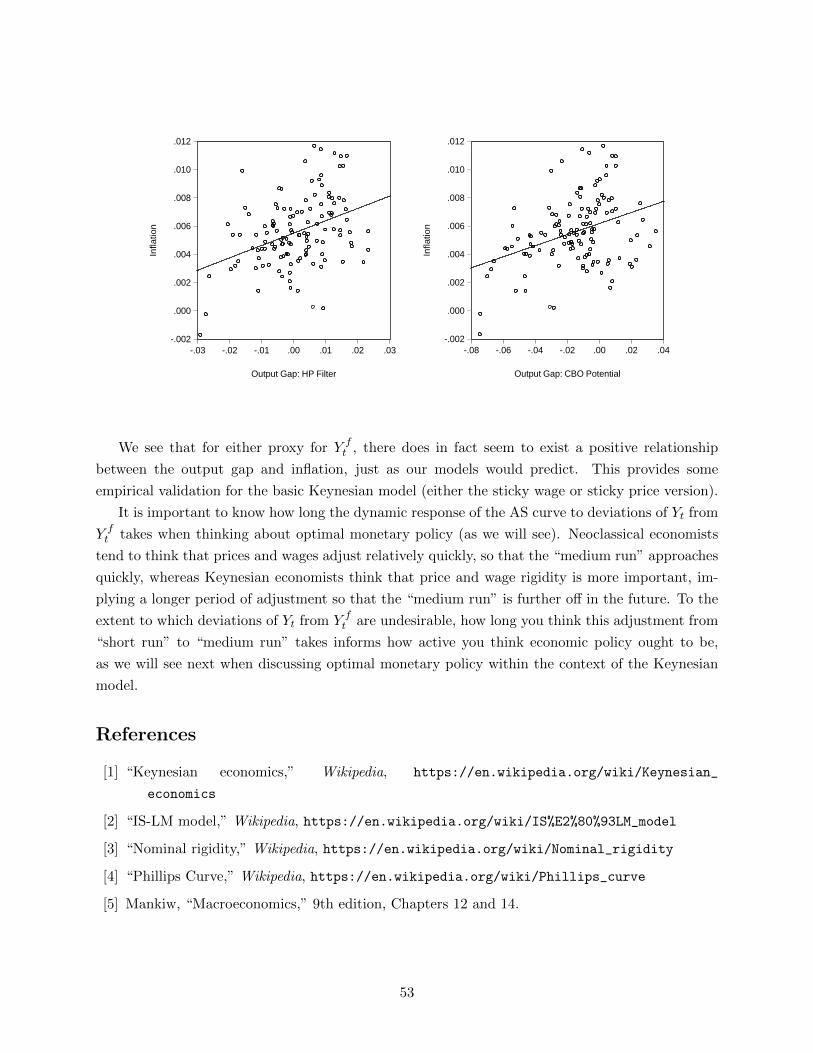
-.002

.000

.002

.004

.006

.008

.010

.012

-.03 -.02 -.01 .00 .01 .02 .03

Output Gap: HP Filter

Infla

tion

-.002

.000

.002

.004

.006

.008

.010

.012

-.08 -.06 -.04 -.02 .00 .02 .04

Output Gap: CBO Potential

Infla

tion

We see that for either proxy for Y ft , there does in fact seem to exist a positive relationship

between the output gap and inflation, just as our models would predict. This provides some

empirical validation for the basic Keynesian model (either the sticky wage or sticky price version).

It is important to know how long the dynamic response of the AS curve to deviations of Yt from

Y ft takes when thinking about optimal monetary policy (as we will see). Neoclassical economists

tend to think that prices and wages adjust relatively quickly, so that the “medium run” approaches

quickly, whereas Keynesian economists think that price and wage rigidity is more important, im-

plying a longer period of adjustment so that the “medium run” is further off in the future. To the

extent to which deviations of Yt from Y ft are undesirable, how long you think this adjustment from

“short run” to “medium run” takes informs how active you think economic policy ought to be,

as we will see next when discussing optimal monetary policy within the context of the Keynesian

model.

References

[1] “Keynesian economics,” Wikipedia, https://en.wikipedia.org/wiki/Keynesian_

economics

[2] “IS-LM model,” Wikipedia, https://en.wikipedia.org/wiki/IS%E2%80%93LM_model

[3] “Nominal rigidity,” Wikipedia, https://en.wikipedia.org/wiki/Nominal_rigidity

[4] “Phillips Curve,” Wikipedia, https://en.wikipedia.org/wiki/Phillips_curve

[5] Mankiw, “Macroeconomics,” 9th edition, Chapters 12 and 14.

53

https://en.wikipedia.org/wiki/Keynesian_economics

https://en.wikipedia.org/wiki/Keynesian_economics

https://en.wikipedia.org/wiki/IS%E2%80%93LM_model

https://en.wikipedia.org/wiki/Nominal_rigidity

https://en.wikipedia.org/wiki/Phillips_curve

Documents

Intermediate Macroeconomics: Keynesian Models...Intermediate Macroeconomics: Keynesian Models Eric Sims University of Notre Dame Fall 2015 1 Introduction At the risk of some oversimpli