Intermediate Macroeconomics:

New Keynesian Model

Eric Sims

University of Notre Dame

Fall 2012

1 Introduction

Among mainstream academic economists and policymakers, the leading alternative to the real

business cycle theory is the New Keynesian model. Whereas the real business cycle model features

monetary neutrality and emphasizes that there should be no active stabilization policy by govern-

ments, the New Keynesian model builds in a friction that generates monetary non-neutrality and

gives rise to a welfare justification for activist economic policies.

New Keynesian economics is sometimes caricatured as being radically different than real business

cycle theory. This caricature is unfair. The New Keynesian model is built from exactly the same

core that our benchmark model is – there are optimizing households and firms, who interact in

markets and whose interactions give rise to equilibrium prices and allocations. There is really only

one fundamental difference in the New Keynesian model relative to the real business cycle model

– nominal prices are assumed to be “sticky.” By “sticky” I simply mean that there exists some

friction that prevents Pt, the money price of goods, from adjusting quickly to changing conditions.

This friction gives rise to monetary non-neutrality and means that the competitive equilibrium

outcome of the economy will, in general, be inefficient.

New Keynesian economics is to be differentiated from “old” Keynesian economics. Old Keyne-

sian economics arose out of the Great Depression, adopting its name from John Maynard Keynes.

Old Keynesian models were typically much more ad hoc than the optimizing models with which

we work and did not feature very serious dynamics. They also tended to emphasize nominal wage

as opposed to price stickiness. Wage and price stickiness both accomplish some of the same things

in the model – they mean that the equilibrium is inefficient and that money is non-neutral. But

nominal wage stickiness implies that real wages may be countercyclical, which is inconsistent with

the data. For this and other reasons, New Keynesian models tend to emphasize price stickiness

(though many of these models also feature wage stickiness too).

Before delving into the details, I’ll give a brief description the main difference relative to our

earlier model. Whereas in our benchmark model output was determined by both supply and

demand, in the New Keynesian sticky price model output is demand determined. We assume that

1

the money price of goods, Pt, is exogenously fixed within period (this is an extreme yet simple form

of price stickiness). The market structure is such that firms are required to produce whatever is

demanded at that fixed price. Changes in the money supply affect the total quantity of nominal

demand for goods; if prices were flexible this would have no effect on the actual amount produced.

But because we assume that firms have to meet demand and because prices are fixed, changes in

the money supply affect real demand.

2 The LM Curve

In this section we introduce a new curve which will be central to our graphical analysis of the New

Keynesian model. It is called the “LM Curve,” where the “L” stands for “liquidity” and the “M”

stands for “money.” Loosely, the “L” part refers to money demand, while the “M” part refers to

money supply. The LM curve shows all (rt, Yt) pairs where the money market is in equilibrium,

taking the price level, Pt, and the money supply, Mt, as given. Traditional Keynesian analysis is

often called the “IS-LM” model. The “IS” stands for “Investment = Saving,” and is identical to

what we have been calling the Y d curve. As we will see below, we can map what we previously did

into the LM curve framework, but the LM curve here is particularly appealing, since it holds the

price level fixed, and we assume that prices are fixed in the New Keynesian framework.

Household optimization generates a demand curve for money which takes the following form:

Mdt = PtM

d(it, Ct)

Since we take expected inflation, πt+1, as given, replace the nominal interest rate using the (ap-

proximate) Fisher relationship:

Mdt = PtM

d(rt + πt+1, Ct)

As before, the money supply is exogenously set by the central bank, M st = Mt.

The only functional difference relative to our earlier model is that the money price of goods is

assumed to be exogenously fixed within period. You can think about this as follows. Suppose that

firms have to post prices before observing any conditions. Then they are committed to producing

whatever is demand at that price for at least one period. Why wouldn’t firms be able to adjust

their price after observing different conditions? The simplest justification is something like a “menu

cost” – suppose that, to change its price, the firm would have to change its menu, which may mean

shutting down production for a period (or at the very least incurring some kind of cost). Implicitly

we are assuming that this cost is sufficiently large that firms will never choose to adjust price within

a period.1 We will call the fixed aggregate price level Pt = P̄ .

1An astute student may realize that there is a slight tension here. If there are many identical firms, then thesefirms have no market power and cannot technically set prices. Hence, a discussion of firms setting prices and thenobserving conditions does not quite seem to work. This is correct. There is a simple way around this that wouldyield identical results if we had more time and more math at our disposal. Just ignore this detail.

2

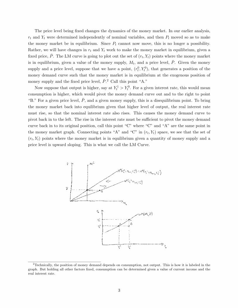
The price level being fixed changes the dynamics of the money market. In our earlier analysis,

rt and Yt were determined independently of nominal variables, and then Pt moved so as to make

the money market be in equilibrium. Since Pt cannot now move, this is no longer a possibility.

Rather, we will have changes in rt and Yt work to make the money market in equilibrium, given a

fixed price, P̄ . The LM curve is going to plot out the set of (rt, Yt) points where the money market

is in equilibrium, given a value of the money supply, Mt, and a price level, P̄ . Given the money

supply and a price level, suppose that we have a point, (r0t , Y0t ), that generates a position of the

money demand curve such that the money market is in equilibrium at the exogenous position of

money supply and the fixed price level, P̄ .2 Call this point “A.”

Now suppose that output is higher, say at Y 1t > Y 0

t . For a given interest rate, this would mean

consumption is higher, which would pivot the money demand curve out and to the right to point

“B.” For a given price level, P̄ , and a given money supply, this is a disequilibrium point. To bring

the money market back into equilibrium given that higher level of output, the real interest rate

must rise, so that the nominal interest rate also rises. This causes the money demand curve to

pivot back in to the left. The rise in the interest rate must be sufficient to pivot the money demand

curve back in to its original position, call this point “C” where “C” and “A” are the same point in

the money market graph. Connecting points “A” and “C” in (rt, Yt) space, we see that the set of

(rt, Yt) points where the money market is in equilibrium given a quantity of money supply and a

price level is upward sloping. This is what we call the LM Curve.

2Technically, the position of money demand depends on consumption, not output. This is how it is labeled in thegraph. But holding all other factors fixed, consumption can be determined given a value of current income and thereal interest rate.

3

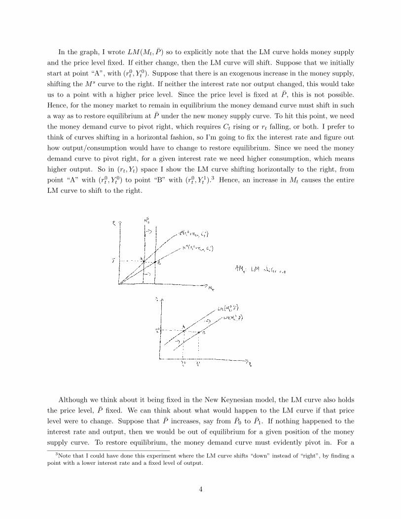
In the graph, I wrote LM(Mt, P̄ ) so to explicitly note that the LM curve holds money supply

and the price level fixed. If either change, then the LM curve will shift. Suppose that we initially

start at point “A”, with (r0t , Y0t ). Suppose that there is an exogenous increase in the money supply,

shifting the M s curve to the right. If neither the interest rate nor output changed, this would take

us to a point with a higher price level. Since the price level is fixed at P̄ , this is not possible.

Hence, for the money market to remain in equilibrium the money demand curve must shift in such

a way as to restore equilibrium at P̄ under the new money supply curve. To hit this point, we need

the money demand curve to pivot right, which requires Ct rising or rt falling, or both. I prefer to

think of curves shifting in a horizontal fashion, so I’m going to fix the interest rate and figure out

how output/consumption would have to change to restore equilibrium. Since we need the money

demand curve to pivot right, for a given interest rate we need higher consumption, which means

higher output. So in (rt, Yt) space I show the LM curve shifting horizontally to the right, from

point “A” with (r0t , Y0t ) to point “B” with (r0t , Y

1t ).3 Hence, an increase in Mt causes the entire

LM curve to shift to the right.

Although we think about it being fixed in the New Keynesian model, the LM curve also holds

the price level, P̄ fixed. We can think about what would happen to the LM curve if that price

level were to change. Suppose that P̄ increases, say from P̄0 to P̄1. If nothing happened to the

interest rate and output, then we would be out of equilibrium for a given position of the money

supply curve. To restore equilibrium, the money demand curve must evidently pivot in. For a

3Note that I could have done this experiment where the LM curve shifts “down” instead of “right”, by finding apoint with a lower interest rate and a fixed level of output.

4

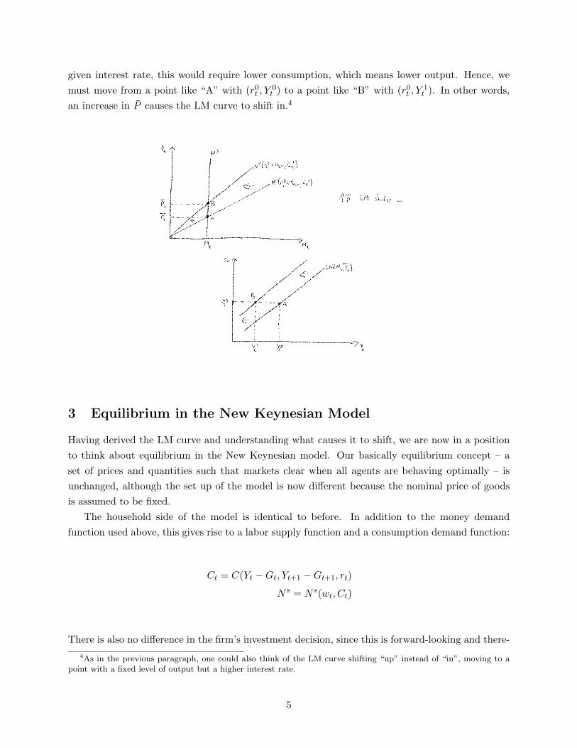
given interest rate, this would require lower consumption, which means lower output. Hence, we

must move from a point like “A” with (r0t , Y0t ) to a point like “B” with (r0t , Y

1t ). In other words,

an increase in P̄ causes the LM curve to shift in.4

3 Equilibrium in the New Keynesian Model

Having derived the LM curve and understanding what causes it to shift, we are now in a position

to think about equilibrium in the New Keynesian model. Our basically equilibrium concept – a

set of prices and quantities such that markets clear when all agents are behaving optimally – is

unchanged, although the set up of the model is now different because the nominal price of goods

is assumed to be fixed.

The household side of the model is identical to before. In addition to the money demand

function used above, this gives rise to a labor supply function and a consumption demand function:

Ct = C(Yt −Gt, Yt+1 −Gt+1, rt)

N s = N s(wt, Ct)

There is also no difference in the firm’s investment decision, since this is forward-looking and there-

4As in the previous paragraph, one could also think of the LM curve shifting “up” instead of “in”, moving to apoint with a fixed level of output but a higher interest rate.

5

fore independent of current demand or the current nominal price. This gives rise to an investment

demand function:

It = I(rt, At+1,Kt)

The total demand for goods and services is the same as before:

Y dt = C(Yt −Gt, Yt+1 −Gt+1, rt) + I(rt, At+1,Kt) +Gt

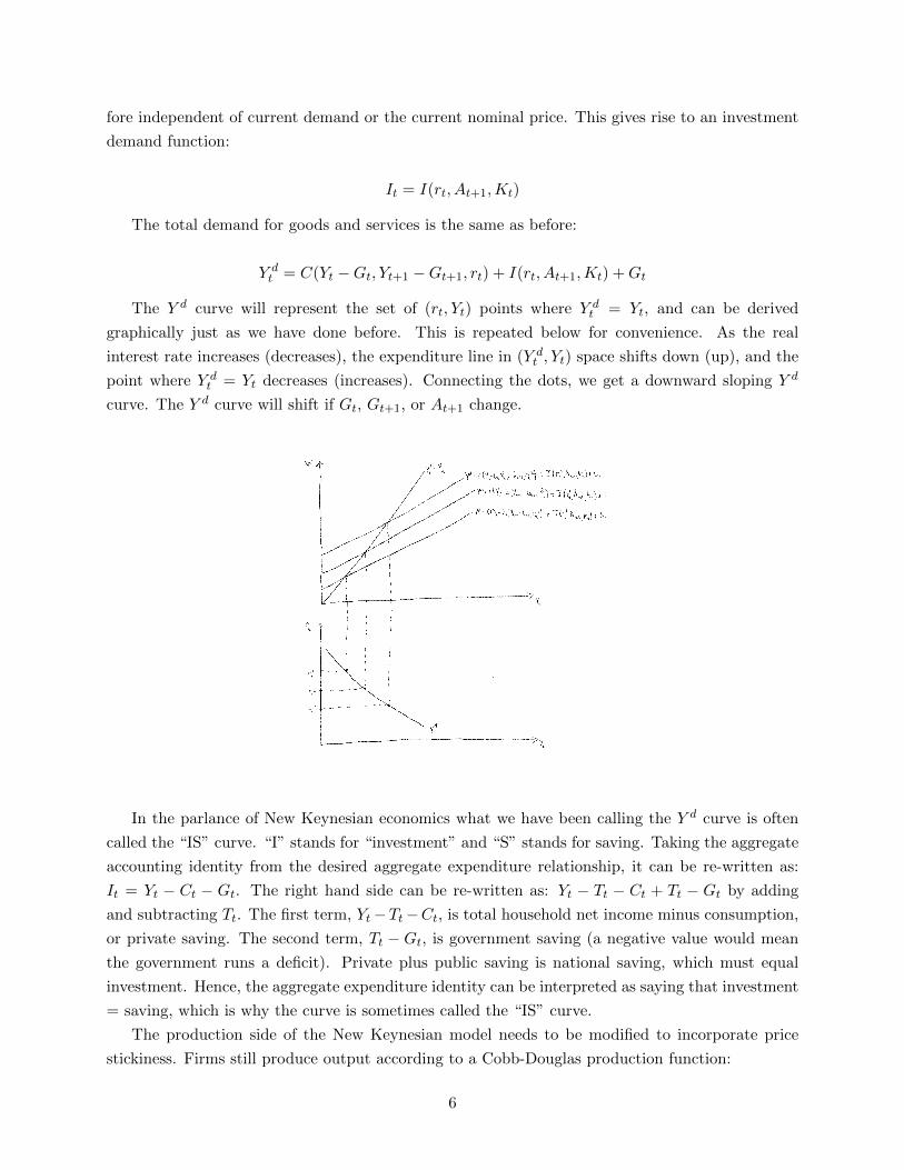
The Y d curve will represent the set of (rt, Yt) points where Y dt = Yt, and can be derived

graphically just as we have done before. This is repeated below for convenience. As the real

interest rate increases (decreases), the expenditure line in (Y dt , Yt) space shifts down (up), and the

point where Y dt = Yt decreases (increases). Connecting the dots, we get a downward sloping Y d

curve. The Y d curve will shift if Gt, Gt+1, or At+1 change.

In the parlance of New Keynesian economics what we have been calling the Y d curve is often

called the “IS” curve. “I” stands for “investment” and “S” stands for saving. Taking the aggregate

accounting identity from the desired aggregate expenditure relationship, it can be re-written as:

It = Yt − Ct − Gt. The right hand side can be re-written as: Yt − Tt − Ct + Tt − Gt by adding

and subtracting Tt. The first term, Yt−Tt−Ct, is total household net income minus consumption,

or private saving. The second term, Tt − Gt, is government saving (a negative value would mean

the government runs a deficit). Private plus public saving is national saving, which must equal

investment. Hence, the aggregate expenditure identity can be interpreted as saying that investment

= saving, which is why the curve is sometimes called the “IS” curve.

The production side of the New Keynesian model needs to be modified to incorporate price

stickiness. Firms still produce output according to a Cobb-Douglas production function:

6

Yt = AtF (Kt, Nt)

The money price of goods is fixed in advance, call this P̄ . As noted in the previous section, we

will think about a sequencing of events whereby firms choose the money price of goods “before”

the period begins, and are committed to sticking with that price through the period. This can be

motivated rigorously through some kind of menu cost. The “rules of the game” are that firms must

produce however much output is demanded given the price they have posted. This means that they

cannot freely choose current employment to maximize profit. Rather, they have to choose Nt (the

only variable factor of production in period t) to produce however much output is demanded. This

means that there is not a normal downward-sloping demand curve for labor as in our earlier setup,

and also means that the Y s curve that we had previously derived is no longer going to be part

of the equilibrium. Put differently, price stickiness essentially obliges the firm to produce however

much output is demanded. There is no optimizing choice of labor input, and hence no Y s curve.

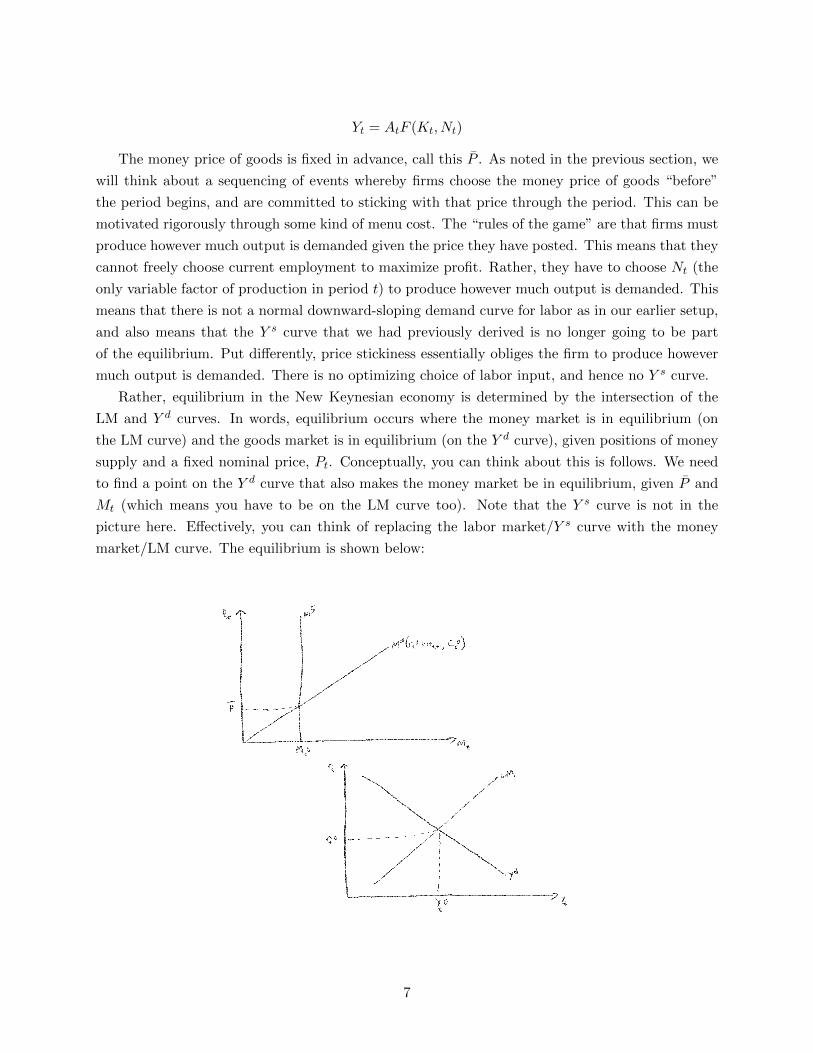
Rather, equilibrium in the New Keynesian economy is determined by the intersection of the

LM and Y d curves. In words, equilibrium occurs where the money market is in equilibrium (on

the LM curve) and the goods market is in equilibrium (on the Y d curve), given positions of money

supply and a fixed nominal price, Pt. Conceptually, you can think about this is follows. We need

to find a point on the Y d curve that also makes the money market be in equilibrium, given P̄ and

Mt (which means you have to be on the LM curve too). Note that the Y s curve is not in the

picture here. Effectively, you can think of replacing the labor market/Y s curve with the money

market/LM curve. The equilibrium is shown below:

7

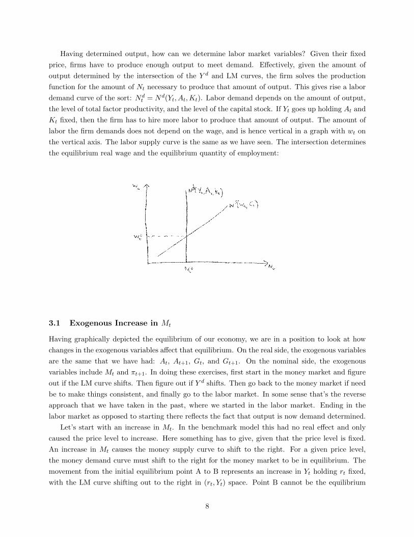
Having determined output, how can we determine labor market variables? Given their fixed

price, firms have to produce enough output to meet demand. Effectively, given the amount of

output determined by the intersection of the Y d and LM curves, the firm solves the production

function for the amount of Nt necessary to produce that amount of output. This gives rise a labor

demand curve of the sort: Ndt = Nd(Yt, At,Kt). Labor demand depends on the amount of output,

the level of total factor productivity, and the level of the capital stock. If Yt goes up holding At and

Kt fixed, then the firm has to hire more labor to produce that amount of output. The amount of

labor the firm demands does not depend on the wage, and is hence vertical in a graph with wt on

the vertical axis. The labor supply curve is the same as we have seen. The intersection determines

the equilibrium real wage and the equilibrium quantity of employment:

3.1 Exogenous Increase in Mt

Having graphically depicted the equilibrium of our economy, we are in a position to look at how

changes in the exogenous variables affect that equilibrium. On the real side, the exogenous variables

are the same that we have had: At, At+1, Gt, and Gt+1. On the nominal side, the exogenous

variables include Mt and πt+1. In doing these exercises, first start in the money market and figure

out if the LM curve shifts. Then figure out if Y d shifts. Then go back to the money market if need

be to make things consistent, and finally go to the labor market. In some sense that’s the reverse

approach that we have taken in the past, where we started in the labor market. Ending in the

labor market as opposed to starting there reflects the fact that output is now demand determined.

Let’s start with an increase in Mt. In the benchmark model this had no real effect and only

caused the price level to increase. Here something has to give, given that the price level is fixed.

An increase in Mt causes the money supply curve to shift to the right. For a given price level,

the money demand curve must shift to the right for the money market to be in equilibrium. The

movement from the initial equilibrium point A to B represents an increase in Yt holding rt fixed,

with the LM curve shifting out to the right in (rt, Yt) space. Point B cannot be the equilibrium

8

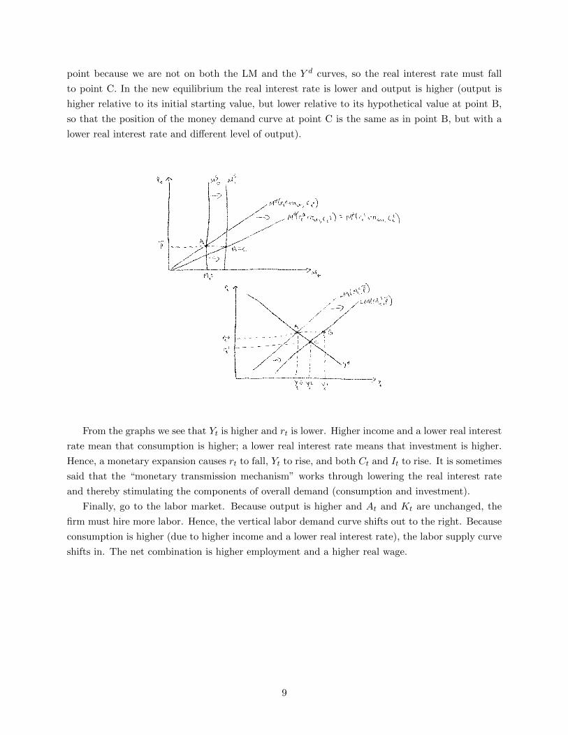
point because we are not on both the LM and the Y d curves, so the real interest rate must fall

to point C. In the new equilibrium the real interest rate is lower and output is higher (output is

higher relative to its initial starting value, but lower relative to its hypothetical value at point B,

so that the position of the money demand curve at point C is the same as in point B, but with a

lower real interest rate and different level of output).

From the graphs we see that Yt is higher and rt is lower. Higher income and a lower real interest

rate mean that consumption is higher; a lower real interest rate means that investment is higher.

Hence, a monetary expansion causes rt to fall, Yt to rise, and both Ct and It to rise. It is sometimes

said that the “monetary transmission mechanism” works through lowering the real interest rate

and thereby stimulating the components of overall demand (consumption and investment).

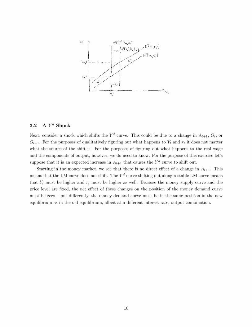
Finally, go to the labor market. Because output is higher and At and Kt are unchanged, the

firm must hire more labor. Hence, the vertical labor demand curve shifts out to the right. Because

consumption is higher (due to higher income and a lower real interest rate), the labor supply curve

shifts in. The net combination is higher employment and a higher real wage.

9

3.2 A Y d Shock

Next, consider a shock which shifts the Y d curve. This could be due to a change in At+1, Gt, or

Gt+1. For the purposes of qualitatively figuring out what happens to Yt and rt it does not matter

what the source of the shift is. For the purposes of figuring out what happens to the real wage

and the components of output, however, we do need to know. For the purpose of this exercise let’s

suppose that it is an expected increase in At+1 that causes the Y d curve to shift out.

Starting in the money market, we see that there is no direct effect of a change in At+1. This

means that the LM curve does not shift. The Y d curve shifting out along a stable LM curve means

that Yt must be higher and rt must be higher as well. Because the money supply curve and the

price level are fixed, the net effect of these changes on the position of the money demand curve

must be zero – put differently, the money demand curve must be in the same position in the new

equilibrium as in the old equilibrium, albeit at a different interest rate, output combination.

10

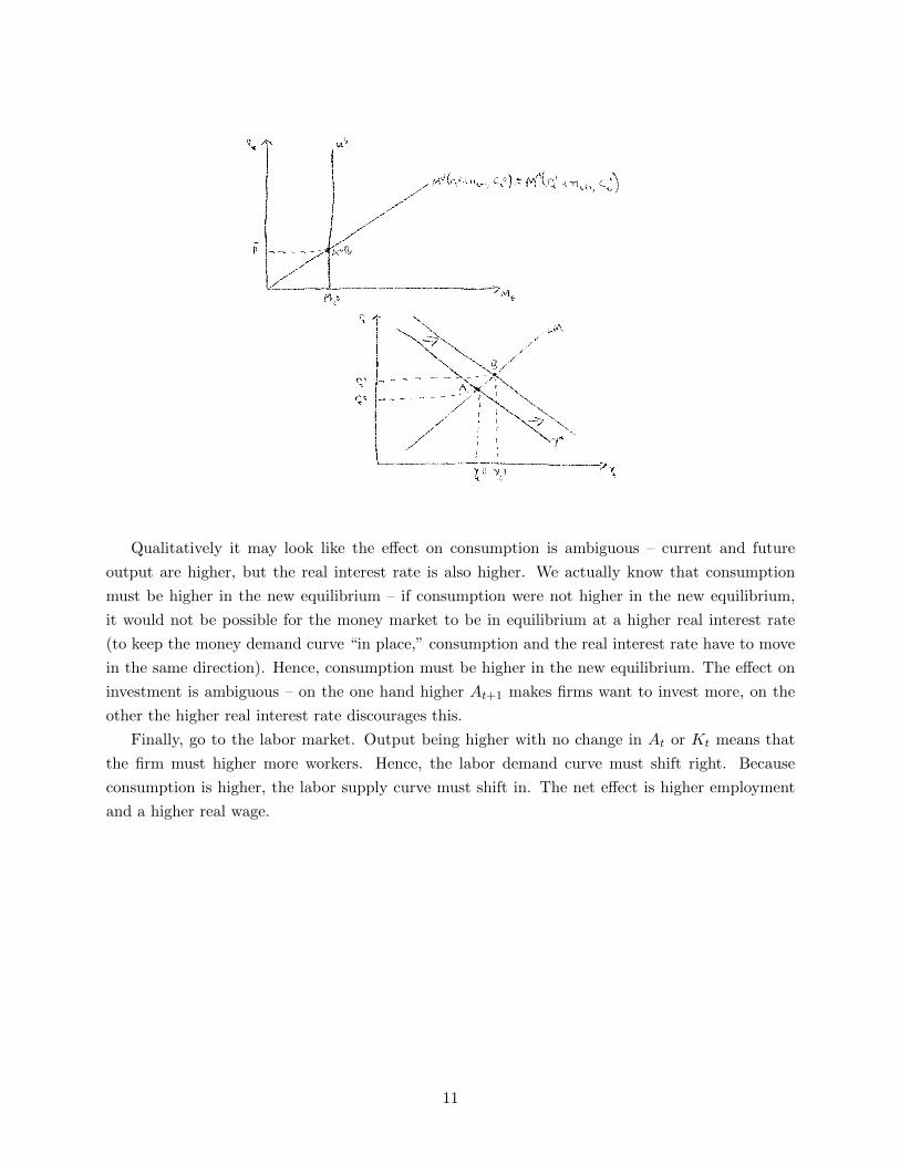
Qualitatively it may look like the effect on consumption is ambiguous – current and future

output are higher, but the real interest rate is also higher. We actually know that consumption

must be higher in the new equilibrium – if consumption were not higher in the new equilibrium,

it would not be possible for the money market to be in equilibrium at a higher real interest rate

(to keep the money demand curve “in place,” consumption and the real interest rate have to move

in the same direction). Hence, consumption must be higher in the new equilibrium. The effect on

investment is ambiguous – on the one hand higher At+1 makes firms want to invest more, on the

other the higher real interest rate discourages this.

Finally, go to the labor market. Output being higher with no change in At or Kt means that

the firm must higher more workers. Hence, the labor demand curve must shift right. Because

consumption is higher, the labor supply curve must shift in. The net effect is higher employment

and a higher real wage.

11

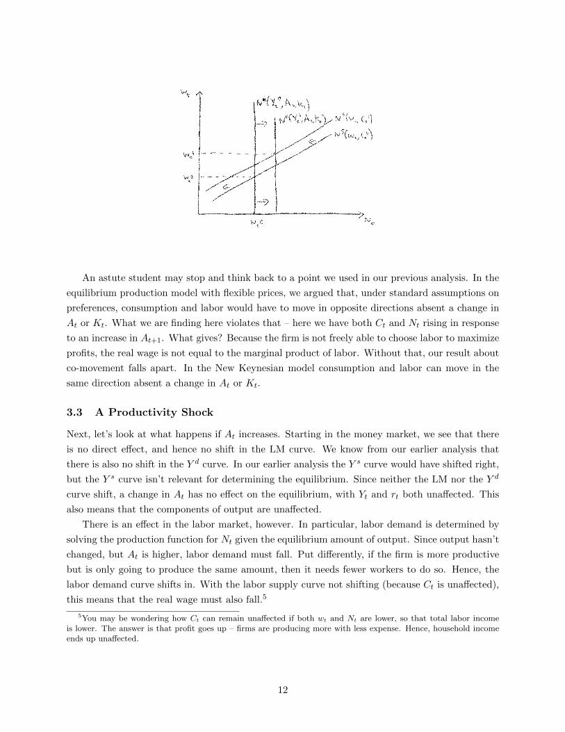
An astute student may stop and think back to a point we used in our previous analysis. In the

equilibrium production model with flexible prices, we argued that, under standard assumptions on

preferences, consumption and labor would have to move in opposite directions absent a change in

At or Kt. What we are finding here violates that – here we have both Ct and Nt rising in response

to an increase in At+1. What gives? Because the firm is not freely able to choose labor to maximize

profits, the real wage is not equal to the marginal product of labor. Without that, our result about

co-movement falls apart. In the New Keynesian model consumption and labor can move in the

same direction absent a change in At or Kt.

3.3 A Productivity Shock

Next, let’s look at what happens if At increases. Starting in the money market, we see that there

is no direct effect, and hence no shift in the LM curve. We know from our earlier analysis that

there is also no shift in the Y d curve. In our earlier analysis the Y s curve would have shifted right,

but the Y s curve isn’t relevant for determining the equilibrium. Since neither the LM nor the Y d

curve shift, a change in At has no effect on the equilibrium, with Yt and rt both unaffected. This

also means that the components of output are unaffected.

There is an effect in the labor market, however. In particular, labor demand is determined by

solving the production function for Nt given the equilibrium amount of output. Since output hasn’t

changed, but At is higher, labor demand must fall. Put differently, if the firm is more productive

but is only going to produce the same amount, then it needs fewer workers to do so. Hence, the

labor demand curve shifts in. With the labor supply curve not shifting (because Ct is unaffected),

this means that the real wage must also fall.5

5You may be wondering how Ct can remain unaffected if both wt and Nt are lower, so that total labor incomeis lower. The answer is that profit goes up – firms are producing more with less expense. Hence, household incomeends up unaffected.

12

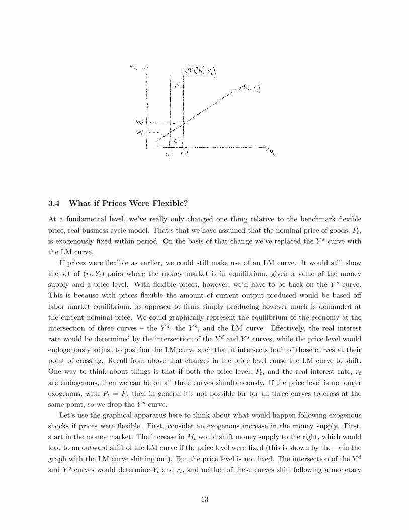
3.4 What if Prices Were Flexible?

At a fundamental level, we’ve really only changed one thing relative to the benchmark flexible

price, real business cycle model. That’s that we have assumed that the nominal price of goods, Pt,

is exogenously fixed within period. On the basis of that change we’ve replaced the Y s curve with

the LM curve.

If prices were flexible as earlier, we could still make use of an LM curve. It would still show

the set of (rt, Yt) pairs where the money market is in equilibrium, given a value of the money

supply and a price level. With flexible prices, however, we’d have to be back on the Y s curve.

This is because with prices flexible the amount of current output produced would be based off

labor market equilibrium, as opposed to firms simply producing however much is demanded at

the current nominal price. We could graphically represent the equilibrium of the economy at the

intersection of three curves – the Y d, the Y s, and the LM curve. Effectively, the real interest

rate would be determined by the intersection of the Y d and Y s curves, while the price level would

endogenously adjust to position the LM curve such that it intersects both of those curves at their

point of crossing. Recall from above that changes in the price level cause the LM curve to shift.

One way to think about things is that if both the price level, Pt, and the real interest rate, rt

are endogenous, then we can be on all three curves simultaneously. If the price level is no longer

exogenous, with Pt = P̄ , then in general it’s not possible for for all three curves to cross at the

same point, so we drop the Y s curve.

Let’s use the graphical apparatus here to think about what would happen following exogenous

shocks if prices were flexible. First, consider an exogenous increase in the money supply. First,

start in the money market. The increase in Mt would shift money supply to the right, which would

lead to an outward shift of the LM curve if the price level were fixed (this is shown by the→ in the

graph with the LM curve shifting out). But the price level is not fixed. The intersection of the Y d

and Y s curves would determine Yt and rt, and neither of these curves shift following a monetary

13

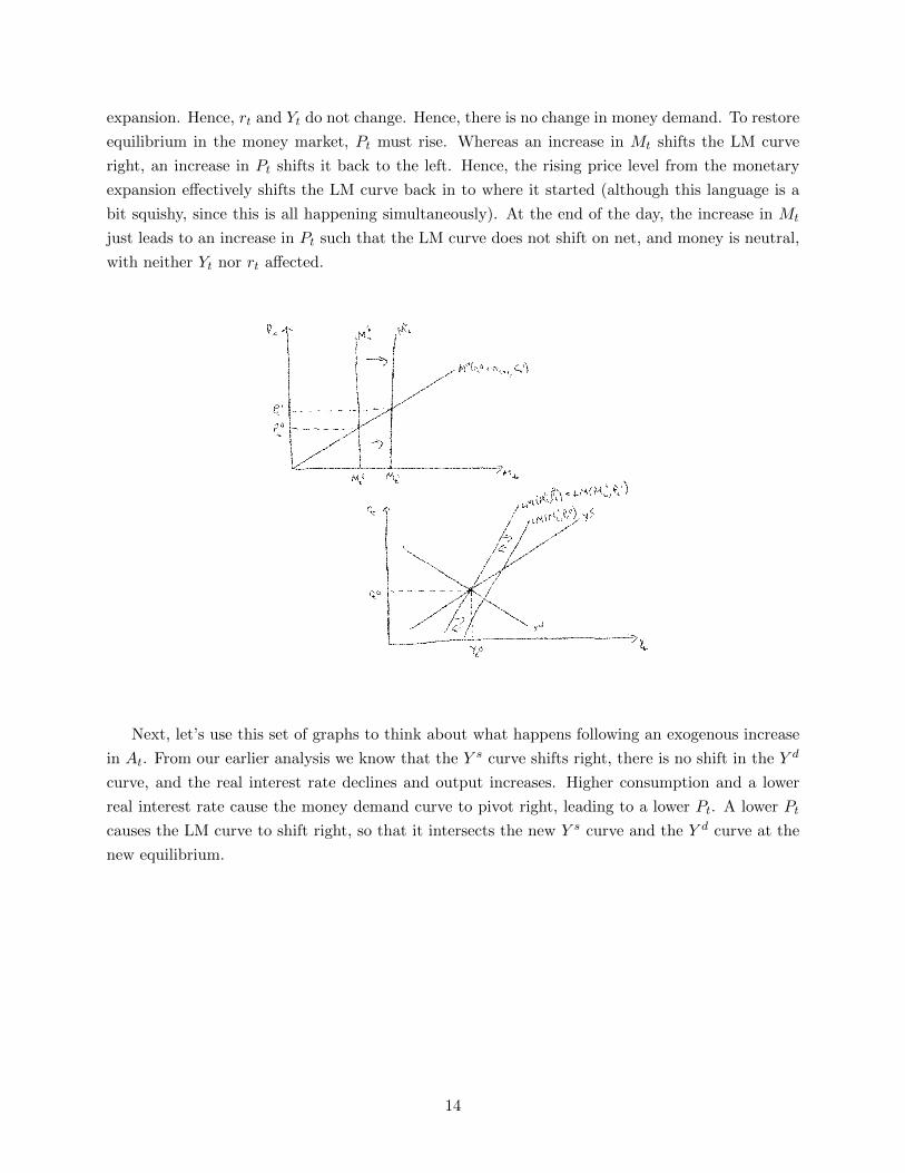
expansion. Hence, rt and Yt do not change. Hence, there is no change in money demand. To restore

equilibrium in the money market, Pt must rise. Whereas an increase in Mt shifts the LM curve

right, an increase in Pt shifts it back to the left. Hence, the rising price level from the monetary

expansion effectively shifts the LM curve back in to where it started (although this language is a

bit squishy, since this is all happening simultaneously). At the end of the day, the increase in Mt

just leads to an increase in Pt such that the LM curve does not shift on net, and money is neutral,

with neither Yt nor rt affected.

Next, let’s use this set of graphs to think about what happens following an exogenous increase

in At. From our earlier analysis we know that the Y s curve shifts right, there is no shift in the Y d

curve, and the real interest rate declines and output increases. Higher consumption and a lower

real interest rate cause the money demand curve to pivot right, leading to a lower Pt. A lower Pt

causes the LM curve to shift right, so that it intersects the new Y s curve and the Y d curve at the

new equilibrium.

14

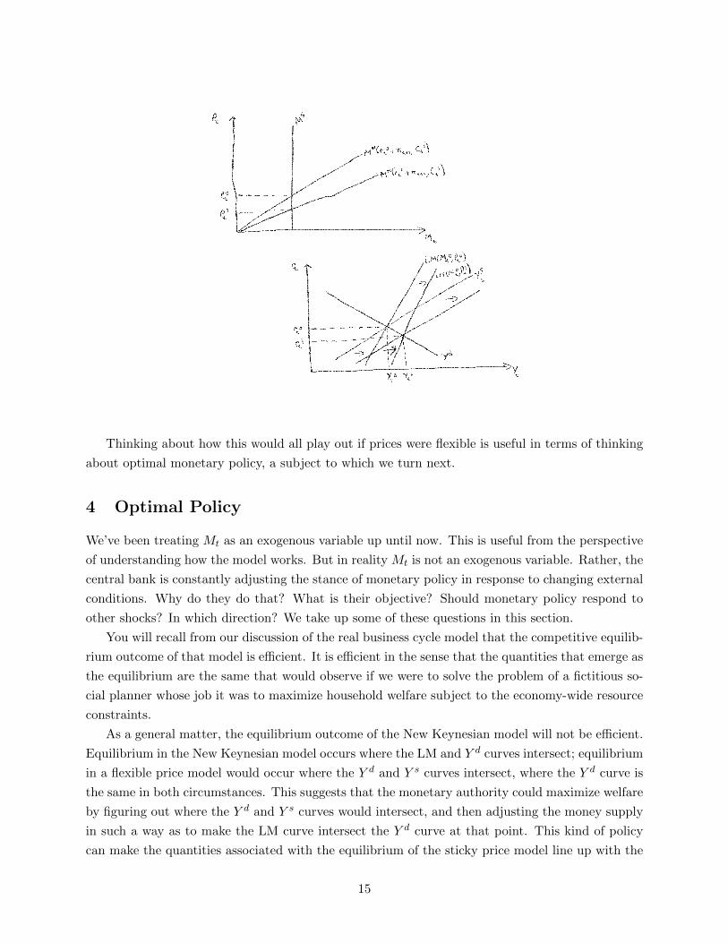
Thinking about how this would all play out if prices were flexible is useful in terms of thinking

about optimal monetary policy, a subject to which we turn next.

4 Optimal Policy

We’ve been treating Mt as an exogenous variable up until now. This is useful from the perspective

of understanding how the model works. But in reality Mt is not an exogenous variable. Rather, the

central bank is constantly adjusting the stance of monetary policy in response to changing external

conditions. Why do they do that? What is their objective? Should monetary policy respond to

other shocks? In which direction? We take up some of these questions in this section.

You will recall from our discussion of the real business cycle model that the competitive equilib-

rium outcome of that model is efficient. It is efficient in the sense that the quantities that emerge as

the equilibrium are the same that would observe if we were to solve the problem of a fictitious so-

cial planner whose job it was to maximize household welfare subject to the economy-wide resource

constraints.

As a general matter, the equilibrium outcome of the New Keynesian model will not be efficient.

Equilibrium in the New Keynesian model occurs where the LM and Y d curves intersect; equilibrium

in a flexible price model would occur where the Y d and Y s curves intersect, where the Y d curve is

the same in both circumstances. This suggests that the monetary authority could maximize welfare

by figuring out where the Y d and Y s curves would intersect, and then adjusting the money supply

in such a way as to make the LM curve intersect the Y d curve at that point. This kind of policy

can make the quantities associated with the equilibrium of the sticky price model line up with the

15

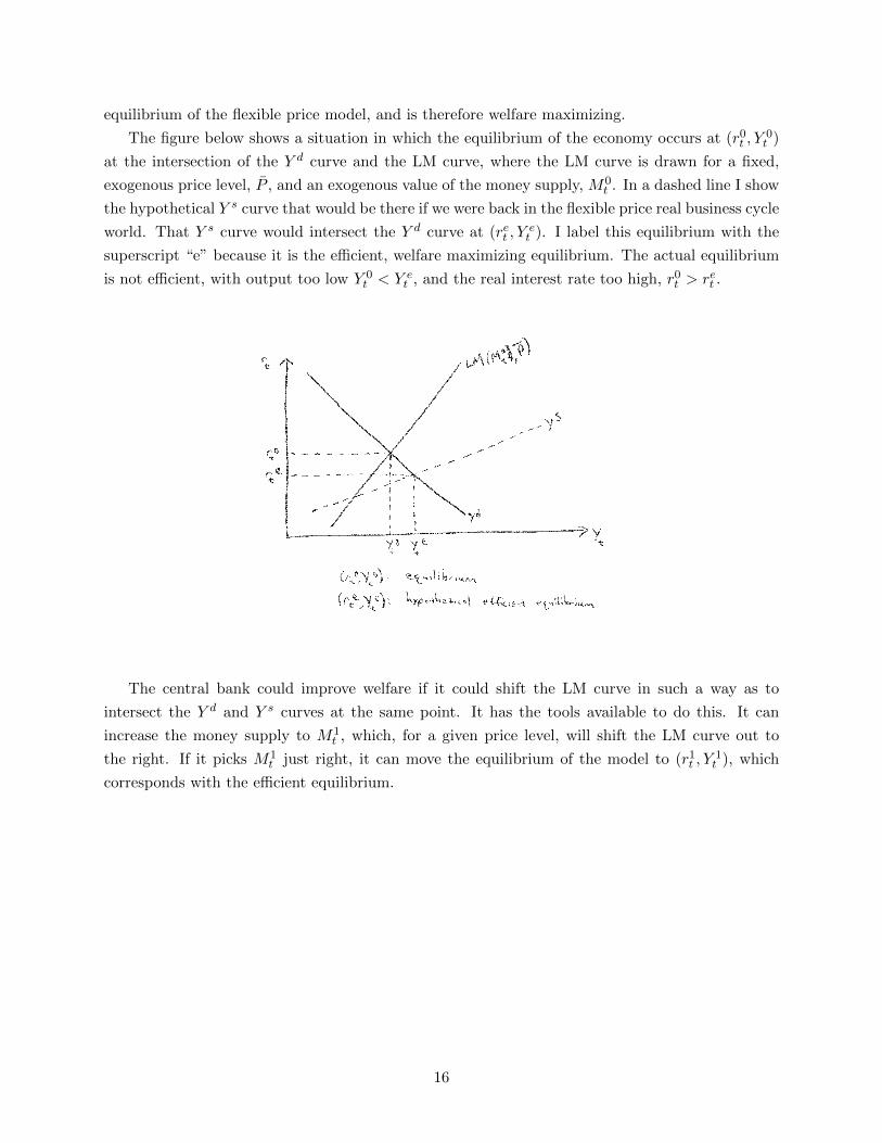
equilibrium of the flexible price model, and is therefore welfare maximizing.

The figure below shows a situation in which the equilibrium of the economy occurs at (r0t , Y0t )

at the intersection of the Y d curve and the LM curve, where the LM curve is drawn for a fixed,

exogenous price level, P̄ , and an exogenous value of the money supply, M0t . In a dashed line I show

the hypothetical Y s curve that would be there if we were back in the flexible price real business cycle

world. That Y s curve would intersect the Y d curve at (ret , Yet ). I label this equilibrium with the

superscript “e” because it is the efficient, welfare maximizing equilibrium. The actual equilibrium

is not efficient, with output too low Y 0t < Y e

t , and the real interest rate too high, r0t > ret .

The central bank could improve welfare if it could shift the LM curve in such a way as to

intersect the Y d and Y s curves at the same point. It has the tools available to do this. It can

increase the money supply to M1t , which, for a given price level, will shift the LM curve out to

the right. If it picks M1t just right, it can move the equilibrium of the model to (r1t , Y

1t ), which

corresponds with the efficient equilibrium.

16

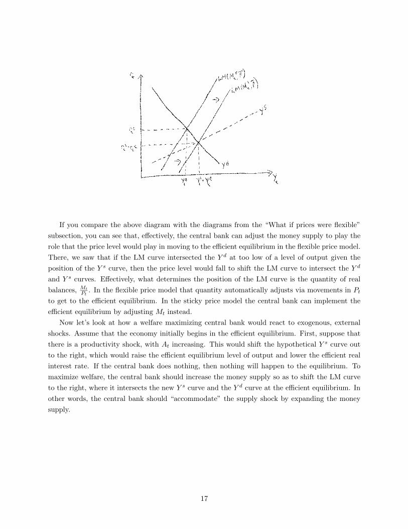
If you compare the above diagram with the diagrams from the “What if prices were flexible”

subsection, you can see that, effectively, the central bank can adjust the money supply to play the

role that the price level would play in moving to the efficient equilibrium in the flexible price model.

There, we saw that if the LM curve intersected the Y d at too low of a level of output given the

position of the Y s curve, then the price level would fall to shift the LM curve to intersect the Y d

and Y s curves. Effectively, what determines the position of the LM curve is the quantity of real

balances, MtPt

. In the flexible price model that quantity automatically adjusts via movements in Pt

to get to the efficient equilibrium. In the sticky price model the central bank can implement the

efficient equilibrium by adjusting Mt instead.

Now let’s look at how a welfare maximizing central bank would react to exogenous, external

shocks. Assume that the economy initially begins in the efficient equilibrium. First, suppose that

there is a productivity shock, with At increasing. This would shift the hypothetical Y s curve out

to the right, which would raise the efficient equilibrium level of output and lower the efficient real

interest rate. If the central bank does nothing, then nothing will happen to the equilibrium. To

maximize welfare, the central bank should increase the money supply so as to shift the LM curve

to the right, where it intersects the new Y s curve and the Y d curve at the efficient equilibrium. In

other words, the central bank should “accommodate” the supply shock by expanding the money

supply.

17

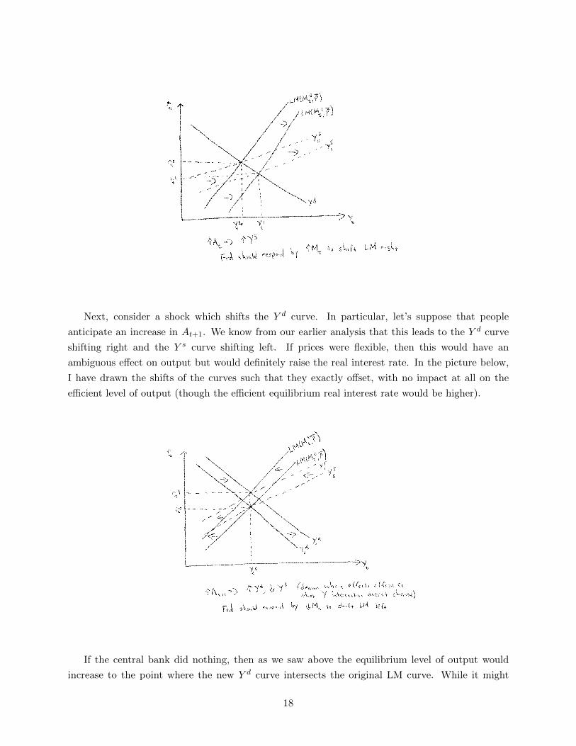
Next, consider a shock which shifts the Y d curve. In particular, let’s suppose that people

anticipate an increase in At+1. We know from our earlier analysis that this leads to the Y d curve

shifting right and the Y s curve shifting left. If prices were flexible, then this would have an

ambiguous effect on output but would definitely raise the real interest rate. In the picture below,

I have drawn the shifts of the curves such that they exactly offset, with no impact at all on the

efficient level of output (though the efficient equilibrium real interest rate would be higher).

If the central bank did nothing, then as we saw above the equilibrium level of output would

increase to the point where the new Y d curve intersects the original LM curve. While it might

18

seem that more output is better, this outcome is not efficient (recall that people get utility from

working too). Output would be too high and the real interest rate too low in that equilibrium. A

welfare maximizing central bank would want to optimally respond to this change by reducing the

money supply, working to shift the LM curve back in to the left. Here the central bank wants to

conduct “countercyclical” policy in the sense of moving the money supply in the opposite direction

of how output would move if it did nothing.

In practice most central banks do not operate in terms of monetary aggregates any more.

Rather, they think of themselves as adjusting interest rates. As we’ve seen, adjusting monetary

aggregates and adjusting interest rates are basically one in the same in this model. One can think

of optimal monetary policy along the following lines in the New Keynesian model. The central bank

wants to adjust interest rates in such a way as to make the equilibrium real interest rate equal the

efficient real interest rate, rt = ret . The efficient real interest rate varies over time due to exogenous

shocks, and so the central bank needs to monitor those shocks, figure out what is happening to ret ,

and adjust the interest rate accordingly.6

In summary, in the New Keynesian model optimal monetary policy calls on the central bank

to endogenously adjust the money supply in such a way as to make the equilibrium coincide with

the hypothetical efficient equilibrium. On paper this seems like a fairly easy task, but in practice

it is not easy. In particular, the central bank must know where the Y s and Y d curves are at any

given point in time to know where to position the LM curve. This requires a pretty sophisticated

and accurate model of the economy and real-time understanding of the shocks which buffet it. If

the central bank has poor information about where the efficient equilibrium would be, or receives

it only after a substantial delay, then activist policies could do more harm than good, moving us

further away from the efficient equilibrium rather than towards it. For this reason, many economists

and politicians propose that central banks should follow relatively simple policy rules as opposed

to using discretion when setting monetary policy. If you go on to take more classes in economics

or go on to graduate school, you will likely encounter this literature in some depth.

5 Empirical Evidence

We talked briefly about the ability of the real business cycle model to match facts about the busi-

ness cycle. What about the ability of the New Keynesian model to match the data? Which model

fits better? Though these are seemingly straightforward questions, there are no easy answers. A

significant complicating factor concerns what monetary policy is doing. As we saw in the previous

section, optimal monetary policy makes the equilibria of the real business cycle and New Keynesian

models observationally equivalent. Hence, when looking at the testable predictions of the two mod-

els, we are (unless otherwise noted) implicitly assuming that monetary policy is not endogenously

reacting to economic conditions.

6As I have noted, technically the central bank can only affect the nominal interest rate. However, to the extent towhich inflation expectations, πt+1, are “well-anchored” (and can thus be interpreted as exogenous and fixed), thenmoving the nominal and the real interest rates are one in the same thing.

19

We saw earlier that the defining feature of the business cycle is broad-based co-movement among

quantities. In the real business cycle context, the only exogenous variable that could generate

this kind of co-movement was At. In the New Keynesian model, changes in Mt and At+1 can

generate co-movement. Another way of putting this is that the real business cycle model emphasizes

supply shocks (changes in At) as the source of business cycles, whereas the New Keynesian model

emphasizes “demand” shocks (changes in the money supply and in expectations of the future, At+1,

which are sometimes called Keynesian “animal spirits”) as the source of the business cycle. Which

explanation holds more water is an empirical question.

A simple test of which theory holds more weight would be to see if changes in Mt have effects

on real variables like output. To the extent to which they do, we can reject the real business

cycle model. In the data, the de-trended component of the money supply and the de-trended

component of output are positively correlated, albeit only mildly so. The positive correlation in

itself is suggestive of real effects of changes in the money supply, but recall that causality could go

both ways. It could be the case that changes in output driven by changes in At lead the central

bank to adjust the money supply (perhaps out of a preference to keep the price level stable), so

that the money supply expands when At, and hence Yt, increase. Hence, a simple correlation may

be suggestive but is not dispositive because causality could go both ways.

A relatively large empirical literature tries to identify exogenous variation in the money supply

(or in other measures of the stance of monetary policy, like interest rates) to look at how those

correlate with changes in output. This literature typically finds that there are real effects of nominal

changes, but that these real effects are (i) relatively small and (ii) relatively short-lived. In a strict

sense this evidence rejects the basic real business cycle framework, but any model that we write

down will be rejected given good enough data, as models are simple abstractions. The fact that

the real effects of nominal shocks appear small and short-lived suggests that the real business cycle

model may not be a poor benchmark, particularly if the frequency of analysis is not too short.

Nevertheless, the fact that there do appear to be real effects of nominal shocks lends evidence to

something like the New Keynesian model.

Another key difference in the predictions of the two models concerns how the economy reacts to

productivity shocks. In the real business cycle framework, changes in At lead to changes in Yt and

almost certainly to movements in Nt of the same direction (though the change in labor is techni-

cally ambiguous, for conventional preference specifications labor input usually rises when At rises).

The New Keynesian model, in contrast, predicts that changes in At should not affect output and

should lead to lower Nt (presuming that the stance of monetary policy is held fixed). One simple

test is to therefore look at the correlations between an empirical measure of At and output and

employment, as we did earlier. There we saw that the Solow residual, or total factor productivity, is

strongly positively correlated with output and employment, which seems to favor the real business

cycle model. Nevertheless, as noted, one criticism of this approach is that employment and capital

may be systematically mis-measured due to unobserved utilization (e.g. you run machines longer

when demand is high, work workers harder when conditions are good, etc.). There are two different

empirical approaches to handling this criticism. One tries to “purify” the Solow residual by using a

20

little bit of economic theory to back out time series for unobserved utilization. This literature has

argued that purified Solow residuals are essentially uncorrelated with output and negatively corre-

lated with employment, consistent with the predictions of the New Keynesian model.7 Another uses

identifying restrictions in a vector autoregression, and argues as well that changes in productivity

lead to employment contractions.8 Though strands point to the New Keynesian model in favor of

the real business cycle model, the results are not without dispute. There are several papers that

challenge the theoretical basis of the approaches used, and argue that technology shocks raise hours

worked, consistent with the real business cycle framework.9 At the end of the day, I think it fair

to say that this is an unsettled empirical question.

Another difference in the implications of the real business cycle and New Keynesian models

revolves around the effects of changes in At+1. Technically, this is a stand in for expected fu-

ture productivity, but you could think about it more widely as being a stand-in for optimism or

pessimism. The real business cycle framework suggests that changes in At+1 cannot be a main

driving force behind the business cycle, because in that model changes in At+1 cannot produce

co-movement: if output goes up following an increase in At+1, then consumption must be going

down. In the New Keynesian framework, in contrast, changes in At+1 can produce broad-based

co-movement. Here I personally have done some research.10 My empirical findings cast doubt on

changes in At+1 as a source of the business cycle – in particular, in my work I find that such changes

lead to (i) small effects on output and (ii) negative co-movement between consumption and hours,

output, and investment. These findings are more in line with the real business cycle model than

with the New Keynesian model.

A final test of the New Keynesian model is to inspect the empirical evidence in support of

the main mechanism in the model, price stickiness. The kind of analysis we have done in class is

necessarily simple, as we simply assumed that the aggregate price level is fixed within period. This

is too large of an abstraction. Some papers, notably Bils and Klenow (2004), look at micro data

from individual firms to look at how often prices change in practice.11 If prices of goods change

infrequently, this is supportive of the price stickiness mechanism at the center of the model. In

practice, prices of most goods change on average once ever 6 or so months. Hence, prices do not

appear perfectly rigid, but they are reasonably flexible.

At the end of the day, the empirical evidence does not compellingly point to either the real

business cycle or the New Keynesian models as the definitive model of the business cycle. This

suggests that more research needs to be done to further refine our theoretical frameworks for

7See Basu, Fernald, and Kimball (2006): “Are Technology Improvements Contractionary?” American EconomicReview.

8See Gali (1999): “Technology, Employment, and the Business Cycle: Do Technology Shocks Explain AggregateFluctuations?” American Economic Review.

9See Chari, Kehoe, and McGrattan (2008): “Are Structural VARs with Long Run Restrictions Useful in DevelopingBusiness Cycle Theory?” Journal of Monetary Economics.

10See Barsky and Sims (2011): “News Shocks and Business Cycles” Journal of Monetary Economics and Barskyand Sims (2012), “Information, Animal Spirits, and the Meaning of Innovations in Consumer Confidence” AmericanEconomic Review.

11See Bils and Klenow (2004), “Some Evidence on the Importance of Sticky Prices” Journal of Political Economy.

21

thinking about economic fluctuations. This does not mean, however, that these two models are

not useful. I think that the insight from real business cycle theory that fluctuations may be the

efficient response to changing condition is quite powerful, and I think that the New Keynesian

model provides a very useful framework for thinking about monetary policy. Whichever model is

better, it makes sense for monetary policy to behave in the way prescribed here. If prices are really

flexible and monetary policy is neutral, then there is not much cost for doing so. If prices are rigid,

then there are welfare gains to be had from this kind of monetary policy.

22