International Conference on Fuzzy Sets and Soft Computing ... · International Conference on Fuzzy Sets and Soft Computing in Economics and Finance FSSCEF 2004 Proceedings Volume

International Conference on Fuzzy Sets and Soft Computing in Economics and Finance

FSSCEF 2004

Proceedings

Volume I

Saint-Petersburg, Russia June 17-20, 2004

ISBN 968-489-028-1 968-489-029-X (Printed version) 968-489-030-3 (Electronic version)

Copyright © 2004 Instituto Mexicano del Petróleo Eje Central Lázaro Cárdenas No. 152 Col. San Bartolo Atepehuacan C.P. 07730 México D.F. Russian Fuzzy Systems Association Vavilova 40, GSP-1, Moscow 119991 Russia http://sedok.narod.ru/fsef.html Editors :

Ildar Batyrshin Janusz Kacprzyk Leonid Sheremetov

Design and Format:

Edgar J. Larios This work is subject to copyright. All rights are reserved. Reproduction of this publication in any form by any electronic or mechanical means (including photocopying, recording or information storage and retrieval) is permitted only under the provisions of the Mexican Federal Copyright Law and the prior permission in writing of Mexican Petroleum Institute. Edited and Formatted in Mexico Printed in Russia (500)

Greetings to Participants in the Conference on Fuzzy Sets and Soft Computing in Economics and Finance

I deeply regret my inability, due to a scheduling conflict, to participate in FSSCEF 2004. I have no doubt that FSSCEF 2004, held in the handsome city of St. Petersburg, will be an important event, providing the participants with opportunity to exchange views and ideas relating to application of fuzzy logic and soft computing in the realms of economics and finance. In my view, it is inevitable that applications of fuzzy logic and soft computing to economics and finance will grow in visibility and importance in the years ahead. The reason is that traditional, bivalent-logic-based approaches, are not a good fit to reality—the reality of pervasive imprecision, uncertainty and partiality of truth. The centrepiece of bivalent logic is the principle of the excluded middle: truth is bivalent, meaning that every proposition is either true or false, with no shades of truth allowed. By contrast, in fuzzy logic everything is, or is allowed to be, a matter of degree. It is this characteristic of fuzzy logic that makes it a much better fit to reality than bivalent logic. In particular, it is this characteristic of fuzzy logic that makes it possible for fuzzy logic to deal with perception-based information. Such information plays an essential role in economics, finance and, more generally in all domains in which human perceptions and emotions are in evidence. With warmest regards to all,

Lotfi A. Zadeh Professor in the Graduate School

Director, Berkeley Initiative in Soft Computing (BISC)

Berkeley, CAMay 2004

Message From the Program Chairs

Following the traditions on organizing international forums in St. Petersburg, the cradle of the Russian Academy of Sciences, the First International Conference on Fuzzy Sets and Soft Computing in Economics and Finance, FSSCEF 2004, was held this year in Northern Palmira. The conference is organized as a platform for exchange of ideas, experiences, and opinions among the academicians, professional engineers and financial community’s practitioners on the applications of soft computing methods and techniques to economics and finance. Conference papers were carefully selected in accordance with best quality international standards. All papers were reviewed by international Program Committee. Finally, the International Program Committee accepted 64 papers from 24 countries. Also Bernard De Baets, Hans De Meyer, Alexander Yazenin, Arkady Borisov, Kaouru Hirota and Toshihiro Kaino accepted the invitation as keynote speakers to present their work.

Soft computing techniques have been applied to a number of systems in economics and finance showing in many cases better performance than competing approaches. At this conference, promising areas such as fuzzy data mining, fuzzy game theory, multi-agent systems, fuzzy and neural modeling have been studied for macro-economic analysis, investment and risk management, time series analysis, portfolio optimization and other applications. Conference Program is composed of 6 sections reflecting the main problem areas and application domains studied in the conference papers: “Fuzzy Data Mining in Economics and Finance”, “Fuzzy Games, Decisions and Expert Systems”, “Fuzzy Mathematical Structures and Graph Theory”, “Multi-Agent Systems and Soft Computing Applications in Economical and Financial Systems”, “Soft Computing Methods in Investment and Risk Analysis and in Portfolio Optimization”, and “Fuzzy Economic and Information Systems”. Many persons contributed numerous hours to organize the Conference. First of all, we would like to thank all the authors and participants for contributing to the Conference and stimulating the technical discussions. Special thanks to the Program and Organizing Committees members and all the institutions supporting this event. We hope that all participants enjoyed the Conference and their stay in St. Petersburg.

Alexey Averkin, Ildar Batyrshin, Janusz Kacprzyk Program Committee Co-Chairs

St. Petersburg

June 2004

FSSCEF 2004 Committees

Honorary Chairman

Lotfi A. Zadeh University of California

Berkeley, USA

Co-Chairs of Program Committee

Alexey Averkin Dorodnicyn Computing Center, Russian Academy of Sciences

Russia

Ildar Batyrshin Mexican Petroleum Institute, Mexico

Institute of Problems of Informatics, Academy of Sciences of Tatarstan, Russia

Janusz Kacprzyk Polish Academy of Sciences

Poland

Co-Chairs of Organizing Committee

Alexey Nedosekin Siemens Business Services Russia

Russia

Lev Utkin St.Petersburg State Forest Technical

Academy Russia

Program Committee

R. Aliev, Azerbaijan A. Altunin, Russia L. Bershtein, Russia J. Bezdek, USA A. Borisov, Latvia J. J. Buckley, USA Ch. Carlsson, Finland J. L. Castro, Spain Sh. Chabdarov, Russia B. De Baets, Begium S. Diakonov, Russia D. Dubois, France V. Emeljanov, Russia A. Eremeev, Russia F. Esteva, Spain B. Fioleau, France J. Fodor, Hungary T. Fukuda, Japan T. Gavrilova, Russia J. Gil-Aluja, Spain Ju. N. Zhuravlev, Russia K. Hirota, Japan R. M. Kachalov, Russia O. Kaynak, Turkey E. Kerre, Belgium G. B. Klejner, Russia E. P. Klement, Austria R. Klempous, Poland G. J. Klir, USA L. T. Koczy, Hungary V. M. Kurejchik, Russia

M. Mares, Czech Republic I. Nasyrov, Russia A. Nedosekin, Russia V. Novak, Czech Republic G. Osipov, Russia P. Osmera, Czech Republic I. Perfilieva, Czech Republic D. Pospelov, Russia H. Prade, France S. V. Prokopchina, Russia A. Ryjov, Russia I. J. Rudas, Hungary T. Rudas, Hungary D. Rutkowska, Poland L. Rutkowski, Poland R. Setiono, Singapore P. Sevastjanov, Poland L. Sheremetov, Mexico P. Sincak, Slovakia R. Slowinski, Poland V. Stefanjuk, Russia R. Suarez, Mexico M. Sugeno, Japan V. Tarasov, Russia I. B. Turksen, Canada L. Utkin, Russia V. Vagin, Russia M. Wagenknecht, Germany R. Yager, USA A. Yazenin, Russia C. Zopounidis, Greece

Invited Speakers

Arkady Borisov Institute of Information Technology

LATVIA

Bernard De Baets Ghent University

BELGIUM

Hans De Meyer Ghent University

BELGIUM

Kaoru Hirota Tokyo Institute of Technology

JAPAN

Toshihiro Kaino Aoyama-Gakuin University

JAPAN

Alexander Yazenin Tver State University

RUSSIA

FSSCEF Sponsorship

Siemens Business Services Russia Mexican Petroleum Institute Russian Fuzzy Systems Association Institute of Problems of Informatics, Academy of Sciences Republic of Tatarstan Kazan State Technological University University of Economics and Finance Economic Faculty of Moscow State University Dorodnicyn Computing Centre of the Russian Academy of Science, Russia International Fuzzy Systems Association IFSA International Association for Fuzzy-Set Management and Economy SIGEF European Society for Fuzzy Logic and Technology EUSFLAT Journal of Audit and Financial Analysis Journal of News of Artificial Intelligence Journal of Mathware and Soft Computing Financial company "Inkastrast"

Table of Contents

VOLUME I INVITED LECTURES A New Approach to Stochastic Dominance ……………………...………………..

De Baets Bernard and De Meyer Hans 3

Optimization with Fuzzy Random Data and its Application in Financial Analysis Yazenin A.V.

16

Machine Learning in Fuzzy Environment ………………………………….……... Borisov Arkady

33

Non-Stochastic-Model Based Finance Engineering ………………………………. Hirota Kaouru and Kaino Toshihiro

35

FUZZY DATA MINING IN ECONOMICS AND FINANCE Plenary Report Mining Fuzzy Association Rules and Networks in Time Series Databases …….....

Batyrshin I., Herrera-Avelar R., Sheremetov L. and Suarez R. 39

Perceptual Time Series Data Mining

A Clear View on Quality Measures for Fuzzy Association Rules ………….……. De Cock Martine, Cornelis Chris and Kerre Etienne

54

Moving Approximations in Time Series Data Mining ………………………….… Batyrshin I., Herrera-Avelar R., Sheremetov L. and Suarez R.

62

On Qualitative Description of Time Series Based on Moving Approximations ….. Batyrshin I., Herrera-Avelar R., Sheremetov L. and Suarez R.

73

Generating Fuzzy Rules for Financial Time Series by Neural Networks with Supervised Competitive Learning Techniques …………………………….………

Marček Dušan

81

Pattern Recognition through Perceptually Important Points in Financial Time Series ………………………………………………………………..……………..

Zaib Gul, Ahmed Uzair and Ali Arshad

89

Fuzzy Classification and Pattern Recognition

Soft Clustering for Funds Management Style Analysis: Out-of-Sample Predictability …………………………………………………………………….....

Lajbcygier Paul and Yahya Asjad

97

Tuning the Fuzzy Classification Models with Various Learning Criteria: the Case of Credit Data Classification ………………………………………………………

Shtovba Serhiy, Pankevich Olga and Dounias Georgios

103

prInvestor: Pattern Recognition Based Financial Time Series Investment System .. Ruta Dymitr

111

On General Scheme of Invariant Clustering Procedures Based on Fuzzy Similarity Relation ………………………..…………………………………………………...

Batyrshin I.Z., Rudas T. and Klimova A.

122

Evolutionary Procedures of Visualization of Multidimensional Data ……….......... Angelica Klimova

130

FUZZY GAMES, DECISIONS AND EXPERT SYSTEMS Plenary Report Vague Utilities in Cooperative Market …………………………………………….

Mareš Milan 143

Fuzzy Games and Decision Making

The Shapley Value for Games on Lattices (L-Fuzzy Games) …………………….. Grabisch Michel

154

Optimal Strategies of Some Symmetric Matrix Games …………………………... De Schuymery Bart, De Meyer Hans and De Baets Bernard

162

On Strict Monotonic t-norms and t-conorms on Ordinal Scales …………………... Batyrshin I.Z. and Batyrshin I.I.

170

Belief Functions and the Imprecise Dirichlet Model ………………………….…... Utkin Lev V.

178

Fuzzy Decision Making Using the Imprecise Dirichlet Model ………………........ Utkin Lev V. and Augustin Thomas

186

Fuzzy Expert Systems

A Fuzzy Expert System for Predicting the Effect of Socio-Economic Status on Noise-Induced Annoyance …………………………………………………………

Zaheeruddin and Jain V. K.

194

The Knowledge Representation Model in Fuzzy Expert Systems Provided by Computing with Words and PRUF Language ……………………………………..

Glova V.I., Anikin I.V., Katasev A.S. and Pheoktistov O.N

202

Decision Trees and Optimization

Construction of Incremental Fuzzy Decision Tree ………………………………... Borisov Arkady and Bikesheva Gulnara

210

Fuzzy Binary Tree Model for European-Style Vanilla Options …………………... Muzzioli Silvia and Reynaerts Huguette

222

Tree-Structured Smooth Transition Regression …………………………………... Correa da Rosa Joel, Veiga Alvaro, Medeiros Marcelo

230

Discrete Dynamic Programming With Outcomes In Fuzzy Ordered Structures ….. Trzaskalik Tadeusz and Sitarz Sebastian

238

FUZZY MATHEMATICAL STRUCTURES AND GRAPH THEORY Plenary Report Fractal Methods of Graphs Partitioning …………………………………………...

Kureichik V.V. and Kureichik V.M. 249

Fuzzy Mathematical Structures

A Method for Definingand Fuzzifying Mathematical Structures …………………. Ionin V.K. and Plesniewicz G.S.

257

On Symmetric MV-Polynomials ………………………………………………...... Di Nola Antonio, Lettieri Ada and Belluce Peter

265

Lattice Products, Bilattices and Some Extensions of Negations, Triangular Norms and Triangular Conorms ………………………………………………...................

Tarassov Valery B.

272

Soft Computing Methods in Graphs Theory and Applications

Definition of Optimum Allocation of the Service Centers ………………………... Bershtein Leonid, Bozhenyuk Alexander and Rozenberg Igor

283

Evolutionary Algorithm of Minimization of Intersections and Flat Piling of the Graph Mathematic Models…………………………………………………............

Gladkov L.A. and Kureichik V.M.

291

Use of a Fuzzy Strategy to Create the Shortest Hamiltonian Cycle ………………. Piech Henryk and Ptak Aleksandra

299

VOLUME II MULTI-AGENT SYSTEMS AND SOFT COMPUTING APPLICATIONS IN ECONOMICAL AND FINANCIAL SYSTEMS Plenary Report Combining Multi-agent Approach with Intelligent Simulation in Resources Flow Management ………………………………………………………………………...

Emelyanov Viktor V.

311

Multi-Agent and Soft Computing Models of Economical Systems

Agent-based Collective Intelligence for Inter-bank Payment Systems ……….......... Rocha-Mier Luis, Villareal Francisco and Sheremetov Leonid

321

Macroeconomic Fuzzy Model of Azerbaijan ………………………………….…… Imanov Q.C., Mamedov F.C and Akbarov R.M.

332

Application of Fuzzy Cognitive Maps to the Political-Economic Problem of Cyprus ………………………………………………………………………………

Neocleous Costas and Schizas Christos

340

Fuzzy Linear Regression Application to the Estimation of Air Transport Demand .. Charfeddine Souhir, Mora-Camino Félix and De Coligny Marc

350

Methodology of the Estimation of Quality of Objects with Complex Structure Under Conditions of Non-Stochastic Uncertainty ………………………………….

Zhelezko Boris A., Siniavskaya Olga A., Ahrameiko Alexey A. And Berbasova Natalya Y.

360

Neural Networks Applications in Economics and Finance

Decision Making in Stock Market with NN and Fuzzy Logic …………………….. Aliev R.A. and Mammadli S. F.

368

The Application of Non-linear Model and Artificial Neural Network to Exchange Rate Forecasting …………………………………………………………………….

Barbouch Rym and Abaoub Ezzeddine

378

Financial Implications of Artificial Neural Networks in Automobile Insurance Underwriting ………………………….……………….……………….……….…..

Kitchens Fred L.

386

A Neural–Fuzzy Approach to Economics Data Classification …………………….. Salakhutdinov R.Z., Ismagilov I. and Rubtsov A.V.

394

SOFT COMPUTING METHODS IN INVESTMENT AND RISK ANALYSIS AND IN PORTFOLIO OPTIMIZATION Plenary Report Portfolio Optimization System (Siemens Business Services Russia) …………........

Alpatsky V.V. and Nedosekin A.O. 403

Soft Computing in Investment and Risk Analysis

Optimal Investment Using Technical Analysis and Fuzzy Logic ………………….. Sevastianov P. and Rozenberg P.

415

Investment Risk Estimation for Arbitrary Fuzzy Factors of Investments Project …. Nedosekin A. and A. Kokosh

423

Robust Selection of Investment Projects …………………………………………... Kuchta Dorota

438

Analyzing the Solvency Status of Brazilian Enterprises with Fuzzy Models ……… Pinto Dias Alves Antonio

446

Opportunities Within the New Basel Capital Accord for Assessing Banking Risk by Means of Soft Computing ……………………………………………………….

Canfora Gerardo, D'Alessandro Vincenzo and Troiano Luigi

457

Risk Analysis in Granular-Information-Based Decision Aid Models ……………... Valishevsky Alexander and Borisov Arkady

466

Fuzzy Portfolio Optimization

A New Approach to Optimizing Portfolio Funding in an Fuzzy Environment ……. Nedosekin Alexey and Korchunov Valentin

474

Comparative Study of Aggregation Methods in Bicriterial Fuzzy Portfolio Selection …………………………………………………………………………….

Sewastianow P. and Jończyk M.

484

On One Method of Portfolio Optimization With Fuzzy Random Data ……………. Grishina Е. N.

493

FUZZY ECONOMIC AND INFORMATION SYSTEMS Plenary Report Towards Human-Consistent Data-Driven Decision Support Systems Via Fuzzy Linguistic Data Summaries …………………………………………………………

Kacprzyk Janusz and Zadrożny Slawomir

501

Fuzzy Information Systems

Information Monitoring Systems as a Tool for Strategic Analysis and Simulation in Business ………………………………………………………………………….

Ryjov Alexander

511

How to Select a Corporate Information System Using Fuzzy Sets ………………... Korolkov Mikhail, Nedosekin Alexey and Segeda Anna

521

Application of a Fuzzy Relational Server to Concurrent Engineering ….…………. Yarushkina Nadezhda

530

Toward Problem of Information Retrieval from Internet ……………..…………… Gilmutdinov R.

538

Fuzzy Models of Economic Systems

New Method for Interval Extension of Leontief’s Input-Output Model Using Parallel Programming ………………………………………………………………

Dymova L., Gonera M., Sevastianov P. and Wyrzykowski R.

549

The Solution of Transport Problem in Fuzzy Statement on the Basis of Platform Anylogic …………………………………………………………………………….

Karpov Yury, Lyubimov Boris and Nedosekin Alexey

557

On the Application of Fuzzy Sets Theory to Russian Banking System Fragility Monitoring ………………………………………………………………………….

Sergei V. Ivliev and Velisava T. Sevrouk

565

A Fuzzy Model of Productivity Control …………………………………………… Piech Henryk and Leks Dariusz

570

Regression Prediction Models with Fuzzy Structure of Adaptive Mechanism ……. Davnis V.V. and Tinyakova V.I.

578

INVITED LECTURES

A New Approach to Stochastic Dominance De Baets Bernard and De Meyer Hans

Optimization with Fuzzy Random Data and its Application in Financial

Analysis Yazenin A.V.

Machine Learning in Fuzzy Environment

Borisov Arkady

Non-Stochastic-Model Based Finance Engineering Hirota Kaouru and Kaino Toshihiro

A New Approach to Stochastic Dominance

Bernard De Baets1 and Hans De Meyer2

1 Department of Applied Mathematics, Biometrics and Process Control,Ghent University, Coupure links 653, B-9000 Gent, Belgium

2 Department of Applied Mathematics and Computer Science,Ghent University, Krijgslaan 281 (S9), B-9000 Gent, Belgium

Summary. We establish a pairwise comparison method for random variables. Thiscomparison results in a probabilistic relation on the given set of random variables.The transitivity of this probabilistic relation is investigated in the case of indepen-dent random variables, as well as when these random variables are pairwisely coupledby means of a copula, more in particular the minimum operator or the ÃLukasiewiczt-norm. A deeper understanding of this transitivity, which can be captured only inthe framework of cycle-transitivity, allows to identify appropriate strict or weak cut-ting levels, depending upon the copula involved, turning the probabilistic relationinto a strict order relation. Using 1/2 as a fixed weak cutting level does not guaran-tee an acyclic relation, but is always one-way compatible with the classical conceptof stochastic dominance. The proposed method can therefore also be seen as a wayof generating graded as well as non-graded variants of that popular concept.

1 Introduction

We denote the joint cumulative distribution function (c.d.f.) of a randomvector (X1, X2, . . . , Xm) as FX1,X2,...,Xm

. This joint c.d.f. characterizes therandom vector almost completely. Nevertheless, it is known from probabilitytheory and statistics that practical considerations often lead one to capturethe properties of the random vector and its joint c.d.f. as much as possibleby means of a restricted number of (numerical) characteristics. The expectedvalue, variance and other (central) moments of the components Xi belong tothe family of characteristics that can be computed from the marginal c.d.f. FXi

solely. A second family consists of characteristics that measure dependenceor association between the components of the random vector. Well-knownmembers of this family are the linear correlation coefficient, also known asPearson’s product-moment correlation coefficient, Kendall’s τ and Spearman’sρ. In general, their computation only requires the knowledge of the bivariatec.d.f. FXi,Xj

. The function C that joins the one-dimensional marginal c.d.f.FXi

and FXjinto the bivariate marginal c.d.f. FXi,Xj

is known as a copula [10]:

FXi,Xj= C(FXi

, FXj) . Although in general not required, we shall assume that

the copula C is the same for all (i, j).Our goal in this contribution is to establish a new method for comparing

the components of a random vector in a pairwise manner. More in particular,with any given random vector we will associate a so-called probabilistic rela-tion. Our main concern is to study the type of transitivity exhibited by thisprobabilistic relation and to analyze to what extent it depends upon the cop-ula that pairwisely couples the components of the random vector. To that end,we need a framework that allows to describe a sufficiently broad range of typesof transitivity. The one that will prove to be the best suited is the frameworkof cycle-transitivity, which has been laid bare by the present authors [2].

This paper is organized as follows. In Section 2, we propose a new methodfor generating a probabilistic relation from a given random vector and indi-cate in what sense this relation generalizes the concept of stochastic domi-nance [9]. One of our aims is to characterize the type of transitivity exhibitedby this relation. To that end, we give a brief introduction to the framework ofcycle-transitivity in Section 3. In Section 4, we consider a random vector withpairwise independent components and analyze the transitivity of the gener-ated probabilistic relation, while in Section 5 we are concerned with randomvectors that have dependent components. In the latter section, we first brieflyreview the important concept of a copula. Then we study two extreme typesof couplings between the components of a random vector, namely by meansof one of the copulas in between which all other copulas are situated, i.e. theminimum operator and the ÃLukasiewicz t-norm [7, 10]. Finally, in Section 6,we explain how the results presented lead to a whole range of methods forcomparing probability distributions and identify proper ways of defining astrict order on them, thus offering valuable alternatives to the usual notion ofstochastic dominance.

2 A method for comparing random variables

An immediate way of comparing two real random variables X and Y is toconsider the probability that the first one takes a value greater than the secondone. Proceeding in this way, a random vector (X1, X2, . . . , Xm) generates aprobabilistic relation (also called reciprocal relation or ipsodual relation), asfollows.

Definition 1. Given a random vector (X1, X2, . . . , Xm), the binary relationQ defined by:

Q(Xi, Xj) = ProbXi > Xj +1

2ProbXi = Xj (1)

is a probabilistic relation, i.e. for all (i, j) it holds that:

Q(Xi, Xj) + Q(Xj , Xi) = 1 .

4 De Baets Baets and De Meyer Hans

Note that Q(X,Y ) is not the probability that X takes a greater value than Y ,since in order to make Q a probabilistic relation, we also take half of the prob-ability of a tie into account. It is clear from this definition that the relationQ can be computed immediately from the bivariate joint cumulative distribu-tions FXi,Xj

as:

Q(Xi, Xj) =

∫x>y

dFXi,Xj(x, y) +

1

2

∫x=y

dFXi,Xj(x, y) . (2)

If we want to further simplify (2), it is appropriate to distinguish between thefollowing two cases. If the random vector is a discrete random vector, then

Q(Xi, Xj) =∑k>l

pXi,Xj(k, l) +

1

2

∑k

pXi,Xj(k, k) , (3)

with pXi,Xjthe joint probability mass function of (Xi, Xj), and if it is a

continuous random vector, then

Q(Xi, Xj) =

∫ +∞

−∞dx

∫ x

−∞fXi,Xj

(x, y) dy , (4)

with fXi,Xjthe joint probability density function of (Xi, Xj). Note that in the

transition from the discrete to the continuous case, the second contributionto Q(Xi, Xj) in (2) has disappeared in (4), since in the latter case it holdsthat ProbXi = Xj = 0.

The probabilistic relation Q generated by a random vector yields a recipefor comparison that takes into account the bivariate joint probability distri-bution function, hence to some extent the pairwise dependence of the com-ponents. The information contained in the probabilistic relation is thereforemuch richer than if for the pairwise comparison of Xi and Xj we would haveused, for instance, only their expected values E[Xi] and E[Xj ].

For two random variables X and Y , one says that X is weakly statisticallypreferred to Y , denoted as X D Y , if Q(X,Y ) ≥ 1/2; if Q(X,Y ) > 1/2, thenone says that X is statistically preferred to Y , denoted X ⊲ Y . Of course, wewould like to know whether the relations D or ⊲ are transitive. To that aim,let us consider the following example of a discrete random vector (X,Y, Z)with three pairwise independent components, uniformly distributed over theinteger sets

DX = 1, 3, 4, 15, 16, 17, DY = 2, 10, 11, 12, 13, 14, DZ = 5, 6, 7, 8, 9, 18 .

We can apply (3) with all joint probability masses equal to 1/36. More pre-cisely, we obtain Q(X,Y ) = 20/36, Q(Y,Z) = 25/36 and Q(X,Z) = 15/36,from which it follows that X ⊲ Y , Y ⊲ Z and Z ⊲ X, and it turns out thatin this case the relation ⊲ (and hence also D) forms a cycle, and hence is nottransitive.

A New Approach to Stochastic Dominance 5

An alternative concept for comparing two random variables, or equiva-lently, two probability distributions, is that of stochastic dominance [9], whichis particularly popular in financial mathematics.

Definition 2. A random variable X with c.d.f. FX weakly stochastically dom-inates in first degree a random variable Y with c.d.f. FY , denoted as X %1 Y ,if it holds that FX ≤ FY . If, moreover, it holds that FX(t) < FY (t), for somet, then it is said that X stochastically dominates in first degree Y , denoted asX ≻1 Y .

Note that, as for any comparison method that relies only upon charac-teristics of the marginal distributions, the stochastic dominance relation %1

does not take into account any effects of the possible pairwise dependenceof the random variables. Moreover, the condition for first-degree stochasticdominance is rather severe, as it requires that the graph of the c.d.f. FX liesbeneath the graph of the c.d.f. FY . The need to relax this condition has led toother types of stochastic dominance, such as second-degree and third-degreestochastic dominance. We will not go into more details here, since we just wantto emphasize the following relationship between weak first-degree stochasticdominance and the relation D.

Proposition 1. For any two random variables X and Y it holds that weakstochastic dominance implies weak statistical preference, i.e. X %1 Y impliesX D Y .

The relation D therefore generalizes weak first-degree stochastic domi-nance %1. Note that the same implication is not true in general for the strictversions ⊲ and ≻1. Since the probabilistic relation Q is a graded alternativeto the crisp relation D, we can interpret it as a graded generalization of weakfirst-degree stochastic dominance. Unfortunately, as shown in the exampleabove, the relation D is not necessarily transitive, while this is obviously thecase for the relation %1. Further on in this paper, we will show how thisshortcoming can be resolved.

3 Cycle -transitivity

Cycle-transitivity was proposed recently by the present authors as a generalframework for studying the transitivity of probabilistic relations [2]. The keyfeature is the cyclic evaluation of transitivity: triangles (i.e. any three points)are visited in a cyclic manner. An upper bound function acting upon the or-dered weights encountered provides an upper bound for the ‘sum minus 1’ ofthese weights. Cycle-transitivity incorporates various types of fuzzy transitiv-ity and stochastic transitivity.


For a probabilistic relation Q on A, we define for all a, b, c the followingquantities:

αabc = min(Q(a, b), Q(b, c), Q(c, a)) ,

βabc = median(Q(a, b), Q(b, c), Q(c, a)) ,

γabc = max(Q(a, b), Q(b, c), Q(c, a)) .

Let us also denote ∆ = (x, y, z) ∈ [0, 1]3 | x ≤ y ≤ z.

Definition 3. A function U : ∆ → R is called an upper bound function if itsatisfies:

(i) U(0, 0, 1) ≥ 0 and U(0, 1, 1) ≥ 1;(ii)for any (α, β, γ) ∈ ∆:

U(α, β, γ) + U(1 − γ, 1 − β, 1 − α) ≥ 1 . (5)

The function L : ∆ → R defined by

L(α, β, γ) = 1 − U(1 − γ, 1 − β, 1 − α) (6)

is called the dual lower bound function of a given upper bound function U .Inequality (5) then simply expresses that L ≤ U .

Definition 4. A probabilistic relation Q on A is called cycle-transitive w.r.t.an upper bound function U if for any (a, b, c) ∈ A3 it holds that

L(αabc, βabc, γabc) ≤ αabc + βabc + γabc − 1 ≤ U(αabc, βabc, γabc) , (7)

where L is the dual lower bound function of U .

Due to the built-in duality, it holds that if (7) is true for some (a, b, c), thenthis is also the case for any permutation of (a, b, c). In practice, it is thereforesufficient to check (7) for a single permutation of any (a, b, c) ∈ A3. Alter-natively, due to the same duality, it is also sufficient to verify the right-handinequality (or equivalently, the left-hand inequality) for two permutations ofany (a, b, c) ∈ A3 (not being cyclic permutations of one another), e.g. (a, b, c)and (c, b, a).

Proposition 2. A probabilistic relation Q on A is cycle-transitive w.r.t. anupper bound function U if for any (a, b, c) ∈ A3 it holds that

αabc + βabc + γabc − 1 ≤ U(αabc, βabc, γabc) . (8)


4 The case of independent random variables

In this section, we consider the case of a random vector with pairwise inde-pendent components Xi. In fact, as is well known in probability theory, thisdoes not mean that the random variables Xi are necessarily mutually inde-pendent. However, since our comparison method only involves the bivariatec.d.f., the distinction between pairwisely and mutually independent randomvariables is superfluous in the present discussion. An important consequence ofthe assumed pairwise independence is that the bivariate distribution functionsbecome factorizable into the univariate marginal distributions, in particularFXi,Xj

= FXiFXj

, for a discrete random vector pXi,Xj= pXi

pXj, and for a

continuous random vector fXi,Xj= fXi

fXj.

The first case in which we have been able to determine the type of tran-sitivity of the probabilistic relation is that of a discrete random vector withpairwise independent components that are uniformly distributed on arbitraryinteger (multi)sets. In this case the components Xi of the random vector canbe regarded as hypothetical dice (with as many faces as elements in the cor-responding multiset), whereas Q(Xi, Xj) can then be seen as the probabilitythat dice Xi wins from dice Xj . Such a discrete uniformly distributed ran-dom vector, together with the generated probabilistic relation, has thereforebeen called a standard discrete dice model [4]. The type of transitivity ofthe probabilistic relation Q can be very neatly described in the framework ofcycle-transitivity [2].

Proposition 3. The probabilistic relation generated by a random vector withpairwise independent components that are uniformly distributed on finite in-teger multisets is cycle-transitive w.r.t. the upper bound function UD definedby:

UD(α, β, γ) = β + γ − βγ .

This type of transitivity is called dice-transitivity.

In [5], the transitivity was investigated in the general case of discrete orcontinuous random vectors with arbitrary independent components. Some-what surprisingly, the above case turned out, as far as transitivity of theprobabilistic relation is concerned, to be generic for the most general situa-tion.

Proposition 4. A random vector with arbitrary pairwise independent compo-nents generates a probabilistic relation that is dice-transitive.

5 The case of dependent random variables

5.1 Joint distribution functions and copulas

In this section, we focus on dependent random variables. We consider the gen-eral case of a random vector (X1, X2, . . . , Xm) with joint c.d.f. FX1,X2,...,Xm

,


to which we associate a probabilistic relation Q, as defined in (1) or, equiva-lently, in (2).

Sklar’s theorem [10, 11] tells us that if a joint c.d.f. FXi,Xjhas marginal

c.d.f. FXiand FXj

, then there exists a copula C such that for all x, y:

FXi,Xj(x, y) = C(FXi

(x), FXj(y)) . (9)

Let us recall that a copula is a binary operation C : [0, 1]2 → [0, 1], that hasneutral element 1 and absorbing element 0 and that satisfies the property ofmoderate growth [10]: for any (x1, x2, y1, y2) ∈ [0, 1]4 it holds that

(x1 ≤ x2 ∧ y1 ≤ y2) ⇒ C(x1, y1) + C(x2, y2) ≥ C(x1, y2) + C(x2, y1) .

A copula C is called stable if for all (x, y) ∈ [0, 1]2 it holds that [8]:

C(x, y) + 1 − C(1 − x, 1 − y) = x + y .

If the random variables Xi and Xj are continuous, then the copula C in(9) is unique; otherwise, C is uniquely determined on Ran(FXi

)×Ran(FXj).

Conversely, if C is a copula and FXiand FXj

are c.d.f., then the function de-fined by (9) is a joint c.d.f. with marginal c.d.f. FXi

and FXj. For independent

random variables, the copula C is the product copula TP (TP(x, y) = xy).In this section we will consider the two extreme copulas in between which

all other copulas are situated, i.e. the ÃLukasiewicz copula TL (TL(x, y) =max(x+y−1, 0), also called the Frechet-Hoeffding lower bound) and the min-imum operator TM (TM(x, y) = min(x, y), also called the Frechet-Hoeffdingupper bound).

In the case of pairwise independent random variables, the computationof Q was done by means of formula (3) (discrete case) or formula (4) (contin-uous case), taking into account that the joint probability mass function (jointprobability density function) is simply the product of the marginal probabilitymass functions (marginal probability density functions). The question ariseswhether for the two extreme cases of dependent random variables, namelycoupled by TM or TL, there exist formulae that simplify the computationof Q.

5.2 The extreme copulas

We first consider the pairwise coupling of components by means of the cop-ula TM:

FXi,Xj(x, y) = min(FXi

(x), FXj(y)) . (10)


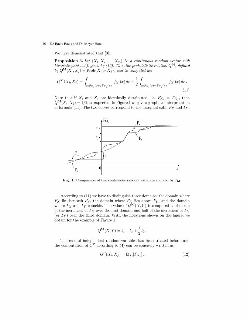
We have demonstrated that [3]:

Proposition 5. Let (X1, X2, . . . , Xm) be a continuous random vector withbivariate joint c.d.f. given by (10). Then the probabilistic relation QM, definedby QM(Xi, Xj) = ProbXi > Xj, can be computed as:

QM(Xi, Xj) =

∫x:FXi

(x)<FXj(x)

fXi(x) dx +

1

2

∫x:FXi

(x)=FXj(x)

fXi(x) dx .

(11)

Note that if Xi and Xj are identically distributed, i.e. FXi= FXj

, thenQM(Xi, Xj) = 1/2, as expected. In Figure 1 we give a graphical interpretationof formula (11). The two curves correspond to the marginal c.d.f. FX and FY .

t1

t2

t3

F( )xFX

FY

FX

FY

0 x

Fig. 1. Comparison of two continuous random variables coupled by TM.

According to (11) we have to distinguish three domains: the domain whereFX lies beneath FY , the domain where FX lies above FY , and the domainwhere FX and FY coincide. The value of QM(X,Y ) is computed as the sumof the increment of FX over the first domain and half of the increment of FX

(or FY ) over the third domain. With the notations shown on the figure, weobtain for the example of Figure 1:

QM(X,Y ) = t1 + t3 +1

2t2 .

The case of independent random variables has been treated before, andthe computation of QP according to (4) can be concisely written as

QP(Xi, Xj) = EXi[FXj

] . (12)


Next, we consider a continuous random vector (X1, X2, . . . , Xm) with ar-bitrary c.d.f. pairwisely coupled by TL:

FXi,Xj(x, y) = max(FXi

(x) + FXj(y) − 1, 0) . (13)

In [3], we have also shown that:

Proposition 6. Let (X1, X2, . . . , Xm) be a continuous random vector withbivariate joint c.d.f. given by (13). Then the probabilistic relation QL, definedby QL(Xi, Xj) = ProbXi > Xj, can be computed as:

QL(Xi, Xj) =

∫x:FXi

(x)+FXj(x)≥1

fXi(x) dx , (14)

or, equivalently:

QL(Xi, Xj) = FXj(u) with u such that FXi

(u) + FXj(u) = 1 . (15)

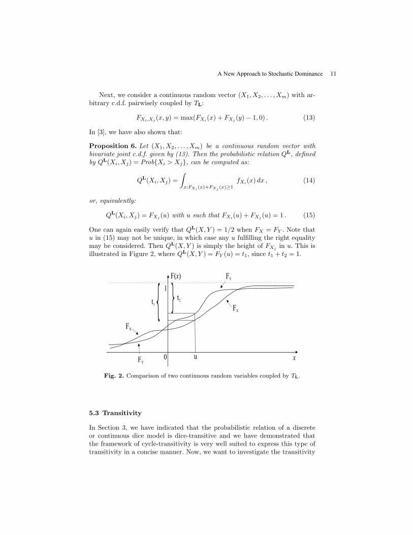
One can again easily verify that QL(X,Y ) = 1/2 when FX = FY . Note thatu in (15) may not be unique, in which case any u fulfilling the right equalitymay be considered. Then QL(X,Y ) is simply the height of FXj

in u. This isillustrated in Figure 2, where QL(X,Y ) = FY (u) = t1, since t1 + t2 = 1.

F( )x

x

FX

FY

t1

t2

FY

FX

0

1

u

Fig. 2. Comparison of two continuous random variables coupled by TL.

5.3 Transitivity

In Section 3, we have indicated that the probabilistic relation of a discreteor continuous dice model is dice-transitive and we have demonstrated thatthe framework of cycle-transitivity is very well suited to express this type oftransitivity in a concise manner. Now, we want to investigate the transitivity


of the probabilistic relation generated by a random vector, with componentspairwisely coupled by a same commutative copula C. We have been able toshow that [3]:

Theorem 1. The probabilistic relation Q generated by a random vector pair-wisely coupled by a commutative copula C is cycle-transitive w.r.t. to the upperbound function UC , defined by:

UC(α, β, γ) = min(β + C(1 − β, γ), γ + C(β, 1 − γ)) . (16)

If C is stable, then

UC(α, β, γ) = β + C(1 − β, γ) = γ + C(β, 1 − γ)) . (17)

Note that without the framework of cycle-transitivity, it would be ex-tremely difficult to describe this type of transitivity in a compact manner.This theorem implies that the relation Q can be seen as a graded alternativeto the notion of stochastic dominance.

The above theorem applies in particular to the Frank t-norm family. ForC = TF

λ , it then holds that the probabilistic relation Q is cycle-transitivew.r.t. the upper bound function UF

λ given by:

UF

λ (α, β, γ) = β + TF

λ (1 − β, γ) = β + γ − TF

1/λ(β, γ) = SF

1/λ(β, γ) . (18)

It is well known that if λ < λ′, then SF

λ < SF

λ′ , which implies that UF

λ > UF

λ′ .Therefore, the lower the value of λ when the random variables are coupledby TF

λ , the weaker the type of transitivity exhibited by the probabilistic re-lation generated by these random variables. In particular, the strongest typeof transitivity is observed when coupling by TL, the weakest when couplingby TM.

Let us discuss the three main copulas:

(i) For C = TL = TF

∞, we obtain from (18) that Q is cycle-transitive w.r.t.the upper bound function UF

∞ given by:

UF

∞(α, β, γ) = max(β, γ) = γ .

This upper bound function has not yet been encountered.(ii) For C = TP = TF

1 , we retrieve the well-known case of independent vari-ables, with

UF

1 (α, β, γ) = β + γ − βγ = UD(α, β, γ) .

(iii)For C = TM = TF

0 , we obtain from (18) that Q is cycle-transitive w.r.t.the upper bound function UF

0 given by:

UF

0 (α, β, γ) = min(β + γ, 1) .

Although not immediately apparent, one can show that cycle-transitivityw.r.t. this upper bound function is equivalent to TL-transitivity.


6 Alternative notions of stochastic dominance

The results from the foregoing sections can also be exploited to come upwith non-graded alternatives to the concept of stochastic dominance. Indeed,consider m random variables X1, X2, . . ., Xm with associated marginal c.d.f.FX1

, FX2, . . ., FXm

, then we can pairwisely couple them (in a virtual manner)by means of a copula C and come up with a probabilistic relation QC on the setof random variables which is cycle-transitive w.r.t. the upper bound functionUC . The latter knowledge allows us to identify more appropriate cutting levelsresulting in a strict order relation.

Theorem 2. Let X1, X2, . . ., Xm be m random variables. For the copulaC = TL, it holds that the binary relation >L defined by

Xi >L Xj ⇔ QL(Xi, Xj) >1

2

is a strict order relation.

For the probabilistic relations QP and QM things are more complicated.

Theorem 3. Let X1, X2, . . ., Xm be m random variables and consider thecopula TP. Let k ∈ N, k ≥ 2.

(i) The binary relation >kP

defined by

Xi >kP

Xj ⇔ QP(Xi, Xj) > 1 − 1

4 cos2(π/(k + 2))

is an asymmetric relation without cycles of length k.(ii)The binary relation >∞

Pdefined by

Xi >∞P

Xj ⇔ QP(Xi, Xj) ≥3

4

is an asymmetric acyclic relation.(iii)The transitive closure >P of >∞

Pis a strict order relation.

Note that the above theorem resolves the dice problem in Section 2. Indeed,

for the given example it only holds that Y >3P

Z, since 2236 <

√5−12 < 23

36 , andthere is no longer a cycle. The appropriate cutting level in this case is nothingelse but the golden section (

√5 − 1)/2.

As can be expected from the above results, it is not easy to identify theappropriate cutting level for a given copula C leading to an acyclic relation.The above theorem expresses that for the product copula TP there exists asequence of cutting levels converging to 3/4 and guaranteeing that the cor-responding relation >k

Pcontains no cycles of length k. Although >∞

Pis not

transitive in general, its transitive closure yields a strict order relation.The same can be done for the copula TM, but the results are less exciting.


Theorem 4. Let X1, X2, . . ., Xm be m random variables and consider thecopula TM. Let k ∈ N, k ≥ 2.

(i) The binary relation >kM

defined by

Xi >kM

Xj ⇔ QM(Xi, Xj) >k − 1

k

is an asymmetric relation without cycles of length k.(ii)The binary relation >M defined by

Xi >M Xj ⇔ QM(Xi, Xj) = 1

is a strict order relation.

The above theorem shows that also for TM there exists a sequence ofcutting levels. Unfortunately, here it converges to 1. It is easily seen that >M

is even more demanding than ≻1. Finally, note that none of the relations >L,>P and >M generalizes the relation ≻1.

7 Conclusion

We have developed a general framework for the pairwise comparison of thecomponents of a random vector, expressed in terms of a probabilistic rela-tion. The framework of cycle-transitivity has proven extremely suitable forcharacterizing the transitivity of this probabilistic relation. This transitivityhas been studied for probabilistic relations generated by pairwise indepen-dent random variables as well as in the case of dependent random variables,although most of the discussion was focused on coupling by TL or TM. Thisstudy has led to graded as well as non-graded alternatives to the classicalconcept of stochastic dominance.

Acknowledgments

H. De Meyer is a Research Director of the Fund for Scientific Research - Flan-ders. This work is supported in part by the Bilateral Scientific and Techno-logical Cooperation Flanders–Hungary BIL00/51 (B-08/2000). Special thanksalso goes to EU COST Action 274 named TARSKI: “Theory and Applicationsof Relational Structures as Knowledge Instruments”.


References

1. B. De Baets and H. De Meyer, Cycle-transitivity versus FG-transitivity, FuzzySets and Systems, submitted.

2. B. De Baets, H. De Meyer, B. De Schuymer and S. Jenei, Cyclic evaluation of

transitivity of reciprocal relations, Social Choice and Welfare, to appear.3. H. De Meyer, B. De Baets and B. De Schuymer, Extreme copulas and the com-

parison of ordered lists, submitted.4. B. De Schuymer, H. De Meyer, B. De Baets and S. Jenei, On the cycle-

transitivity of the dice model, Theory and Decision 54 (2003), 264–285.5. B. De Schuymer, H. De Meyer and B. De Baets, Cycle-transitive comparison of

independent random variables, submitted.6. J. Garcıa-Lapresta and B. Llamazares, Aggregation of fuzzy preferences: some

rules of the mean, Social Choice and Welfare 17 (2000), 673–690.7. E. Klement, R. Mesiar and E. Pap, Triangular Norms, Trends in Logic, Studia

Logica Library, Vol. 8, Kluwer Academic Publishers, Dordrecht, 2000.8. E. Klement, R. Mesiar and E. Pap, Invariant copulas, Kybernetika 38 (2002),

275–285.9. H. Levy, Stochastic Dominance, Kluwer Academic Publishers, MA, 1998.

10. R. Nelsen, An Introduction to Copulas, Lecture Notes in Statistics, Vol. 139,Springer-Verlag, New York, 1998.

11. A. Sklar, Fonctions de repartition a n dimensions et leurs marges, Publ. Inst.Statist. Univ. Paris 8 (1959), 229–231.


Optimization with fuzzy random data and its application in financial analysis1

A.V. Yazenin

Computer Science Department, Tver State University, Ul. Zhelyabova 33, 170000 Tver, Russia. [email protected].

Abstract.

In the present paper an approaches to the definition of numerical charac-teristics of fuzzy random variables are analyzed and proposed. Appropriate methods of its calculation, in particular within the framework of shift-scaled representation are obtained. Principles of decision making in fuzzy random environment are formulated. Possibilistic-probabilistic models of portfolio analysis problems and general methods for its solving are devel-oped.

Keywords:

Fuzzy random variable, variance and covariance, possibilistic-probabilistic optimization, financial analysis, portfolio selection

Introduction

Fuzzy random variable is a mathematical model of a probabilistic ex-periment with fuzzy outcome. A number of works are devoted to its defini-tion and investigation of its properties – see, for example [1-4] and other. Besides of proper definition of fuzzy random variable, definitions of its expected value are introduced, its properties are investigated and methods ____________________________________________________________ 1 This work was carried out with financial support of RFBR (project No. 02-01-011137)

of calculation are proposed for different particular cases. However, series of important questions such as a manner of representation of fuzzy random variable, definition of variance and covariance, development of calculus of fuzzy random variables are still remains open. This circumstance evidently restrains an application of fuzzy random variables for the modeling of such combined type of uncertainty in decision making.

Here we present results that reflect latest achievements in formulated above directions of researching. Representation of a fuzzy random variable allowing to explicate random and fuzzy factors and build an appropriate calculus is considered. Approaches to definition of the moments of the second order are analyzed. Developed mathematical apparatus and fuzzy random variable calculus are oriented for its application in problems of op-timization and decision making, in particular in portfolio analysis prob-lems.

The content of the paper is as follows. In the first part the definition of the possibilistic variable is given. In

common it inherits S. Nahmias approach [1, 2]. The possible value distri-butions of fuzzy random variables are introduced along with several con-ceptions necessary for following formation. In possibilistic-probabilistic context the definition of a fuzzy random variable and its interpretation are given.

In the second part method of representation of a fuzzy random variable on the ground of shift-scaled family of possibilistic distributions is consid-ered. For such fuzzy random variable representation the calculation meth-ods for expected value, variance and correlation coefficients with one of the approaches to its definition are obtained. As an illustration, it is shown how the calculations can be carried out in general with shift-scaled repre-sentation in the class of symmetrical triangular possibilistic distributions.

In the third part the principles and criteria of decision making in fuzzy random environment are formulated.

The fourth section is devoted to developing portfolio analysis problem models with fuzzy random data and to methods of their solution.

In conclusion the represented results and course of further researches are considered.

1. Fuzzy random variables and their distributions in possibility-probability context

Following [1,2] we introduce necessary definitions and notations.

Optimization with fuzzy random data and its application in financial analysis 17

Let be a set of elements denoted as Γ )(, ΓΡΓ∈γ is a power set of

, Γ nE denotes the n – dimensional Euclidean space.

Definition 1. A possibility measure is a set function with properties:

1)(: E→ΓΡπ

1. ;1,00 =Γ=/ ππ 2. ,sup iIiIi

i AA ππ∈∈

=U

for any index set I and ( )ΓΡ∈iA .

Triplet ( )( )π,, ΓΡΓ is a possibilistic space.

Definition 2. A possibilistic (fuzzy) variable is a mapping 1: EZ →Γ . Distribution of possibilistic values of variable Z is function

, defined as 11: EEZ →µ .,)(:)( 1EzzZzZ ∈∀=Γ∈= γγπµ

( )zZµ is a possibility that variable Z may accept value z . From the last definition and possibility measure properties it follows

a) ( ) ;,10 1EzzZ ∈∀≤≤ µ b) ( ) .1sup1

=∈

zZEzµ

Definition 3 The support of a possibilistic variable . Z is given by

supp ( ) ( ) .0/1 >∈= zEzZ Zµ Definition 4. r -level set of a fuzzy variable Z is given by

( ) ( ]1,0,1 ∈≥∈= rrzEzZ Zr µ/ . A necessity measure ν is a dual concept notion to a possibility measure

and defined as ( ) ( )cAA πν −= 1( )Γ∈P

, where " means the complement of a set .

"cA

Taking into consideration results [2], [5], give the definition of a fuzzy random variable and its interpretation.

Let ( )ΡΒΩ ,, be a probability space. Definition 5. Fuzzy random variable X is a real function

such that for any fixed ( ) ,:, 1EX →Γ×Ω⋅⋅ Γ∈γ ( )γωγ ,XX =

is a random variable on ( )ΡΒΩ ,, . From the forecited definition follow two interpretations.

18 Yazenin A.V.

For a fixed Ω∈ω we get a fuzzy variable ( )γωω ,XX = . The values of a random variable are fuzzy variables with probability distribu-tions ( )ωµ ,xX .

For a fixed γ can be considered as a random variable with possi-

bility defined by a possibility measure. γX

Everything becomes clear when distribution ( )ωµ ,xX is defined as in case of fuzzy variable:

( ) ( ) 1,:, ExxXxX ∈∀=Γ∈= γωγπωµ . For each ω corresponds possibilistic distribution that is a random

choice of an expert who gives an indefinite subjective estimation with cer-tain amount.

X is a random variable for a fixed γ , but we are not sure in its distri-bution value.

In the context of decision making expected value plays crucial role in explanation of random information. The expected value ( ) γω ,XE of

a random variable ( )γω ,X can be defined in different ways. We define distribution of a random variable expected value according to

[2] through averaged random variable:

( ) ( ) 1,: ExxXExEX ∈∀=Γ∈= γωγπµ . It’s easy to show an expected value of a fuzzy random variable defined

this way has the basic properties of random variable expected value.

2. Fuzzy random variables presentation and calculation of their characteristics

Let’s consider fuzzy random variable ( )γω ,X . Presentation [6] is in-teresting for applications: ( ) ( ) ( ) ( ),, 0 γωσωγω XaX += (2.1)

where ( ) ( )ωσω ,a)Ρ,

are random variables defined on probability space

, have finite moments of the second order, and ( ΒΩ, ( )γ0X( )

is a

fuzzy (possibilistic) variable defined on possibilistic space ( )π,, ΓΡΓ .


To simplify demonstration of basic ideas suppose ( ),1,00 TrX ∈ that

is has triangular distribution function 0X

( )

>

≤−=

.1,0

,1,10 t

tttXµ (2.2)

From (2.2) follows a fuzzy random variable has modal value and fuzziness coefficient equal, respectively, to 1 and 0.

0X

Presentation (2.1) is shift-scale presentation of a fuzzy random variable. ( ) ( )ωσω ,a are shift and scale parameters which are modal value and

fuzziness coefficient of a fuzzy random variable ( ) ( ) ( )( )ωσωγωω ,, aTrXX ∈= .

Let ( ) ( ) ., 00 σσ == EaaE000 Xa

Then according to [1,2]

( )XE σ+= and

( ) ( )( ) ./ 1000

Etatt XEX ∈∀−= σµµ

Solving applied problems we are interested not only in expected value but also in variance and covariance of fuzzy random variables. There exist at least two approaches to their definition. The characteristics are fuzzy within the first approach [6] and nonfuzzy within the second one[7].

Consider the first approach. Variance and covariance are defined by probability theory formulae. Using presentation (2.1) we obtain formula for variance of a fuzzy random variable (XD ) ( )γω ,X as function of fuzzy variable : 0X( ) ( ) ( )

( )( ) ( ) ( ) ( )

( ) ( )( )

( ) ( ) ( )( ) )3.2(.,cov,cov

,cov222

0

200

2000

200000

σσσ

σσσ

σσσσ

σσσ

DaDaD

DaXD

XDXaaDXaaE

XaXaEXaDXD

−+

+=

=++==−+−=

=−−+=+=

Let

( ) ( )( )

( ) ( ) (( )

)σ

σσσσσ

DaDaDC

DaCDC ,cov,,cov;

2

3221

−=== .

20 Yazenin A.V.

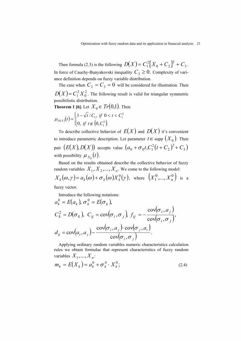
Then formula (2.3) is the following ( ) [ ] 32

2021 CCXCXD ++=

.03 ≥C.

In force of Cauchy-Bunyakovski inequality Complexity of vari-ance definition depends on fuzzy variable distribution.

The case when 032 == C2

C will be considered for illustration. Then

. The following result is valid for triangular symmetric possibilistic distribution. ( ) 0

21 XCXD =

Theorem 1 [6]. Let ( )1,00 TrX ∈ . Then

( )( ) ( )

∉

<<−=

.,0,0

0,/12

1

211

Ctif

CtifCttXDµ

To describe collective behavior of ( )XE and ( )XD it’s convenient to introduce parametric description. Let parameter ∈t supp ( )0X . Then

pair accepts value ( ) ( )( XDXE , ) ( ( ) )30 C+σ 22C +2

1, tCt0a +

with possibility (tX 0)µ .

Based on the results obtained describe the collective behavior of fuzzy random variables . We come to the following model: nXXX ,,..., 21

( ) ( ) ( ) ( )γωσωγω 0, kkkk XaX += , where ( )001 ,..., nXX is a

fuzzy vector.

Introduce the following notations:

( ) ( ),, 00kkkk EaEa σσ ==

( ) ( ) ( )( ) ,,cov

,cov,,cov,2

ji

jiijjiijkk

afCDC

σσ

σσσσ −===

( ) ( ) ( )( )ji

ijjijiij

aaaad

σσσσ

,cov,cov,cov

,cov⋅

−= .

Applying ordinary random variables numeric characteristics calculation rules we obtain formulae that represent characteristics of fuzzy random variables : nXX ,...,1

( ) ;000kkkkk XaXEm ⋅+== σ (2.4)


( ) [ ] ;2022

kkkkkkkk dfXCXDD ++== (2.5)

( ) ( )( ))6.2(

,cov ijjiojij

oiijjiij dfXfXCXX +−−==Σ

Let be a mean vector, ( nmmm ,,...1= ) ( )ijΣ=Σ be a covari-

ance matrix of fuzzy vector ( ) ( )( )γωγω ,,,...,1 nXX . Calculate col-

lective possibilistic distribution of m and Σ . Let ( )nt,t ,...1t = be a

point from a set of possible values of a fuzzy vector

( )001 ,..., nX0 XX = . According to forecited results pair ( )Σ,m ac-

cepts value ( ) ( )( )ttm Σ, with possibility ( )tX 0µ . Elements and

can be calculated by formulae (2.4) - (2.6).

(tmk )( )tijΣ

Actually, as then ,, 00jjii tXtX ==

( ) ( ) ( )( ) ijjijij ijiijkkkk dftftCttatm +−−=⋅+= ∑;00 σ .

If elements of t e vector are min-related [5] then h 0X( ) ( ) iXniX

tt oi

µµ≤≤

=1min0 .

The second approach. Omitting all the technical details connected with fuzzy random variable values definition in space [7] in accepted notation, the corresponding formulae are:

∞L

( ) ( ) ( )( )( ( ) ( )( ) ,,cov,cov21,cov

1

0

drrYrXrYrXYX ++−− += ∫ ωωωω )

where ( ) ( ) ( ) )(,,, rYrXrYrX ++−−ωωωω

ωω YX ,( )XX ,cov=

are r–level set endpoints of

fuzzy variables respectively. It’s obvious variance

and moments of the second order are without fuzziness. It’s important that the definition methods of the second order moments in the first and second approaches are different in principle. In the first approach we identify possibility distribution and in the second one we make numeric calculations.

( )XD

22 Yazenin A.V.

3. Possibility-probability optimization models and decision making

Within fuzzy random data functions that form goals and restrictions of decision making problem make sense of mapping

( ) miEWRi ,0,:,, 1 =→Γ×Ω×⋅⋅⋅n

, where W is a set of acceptable

solutions, EW . Thus, a set of acceptable outcomes can be obtained by combination of solution set elements with elements of random and fuzzy parameter sets. That’s why any concrete solution can’t be directly connected either with goal achievement degree no with restriction system execution degree.

⊂

Existence of two different types of uncertainty in efficiency function complexifys reasoning and formalization of solution selection optimality principles. However decision making procedure based on expected possi-bility principle is quite natural. Its content is elimination of two types of uncertainty that is a realization of two types of decision making principles [5], [8,9]: averaging of fuzzy random data that allows to get to decision mak-

ing problem with fuzzy data; choice of optimal solution with more possible values of fuzzy pa-

rameters or with possibility not lower than preset level. Adequate mean of suggested optimality principle formalization is a

mathematical apparatus of fuzzy random variables. Let τ be a possibility or necessity measure that is νπτ ,∈ . Taking

into consideration stated decision making principles we came to the fol-lowing optimization problem settings within fuzzy random factors.

Problem of maximizing goal achievement measure with liner possibility (necessity) restrictions

( ) max,0,, 00 →ℜγωτ wER ( )

∈=≥ℜ

.,,1,0,,

WwmiawER iii γωτ


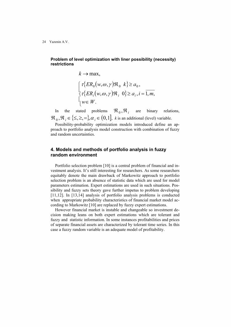
Problem of level optimization with liner possibility (necessity) restrictions

max,→k

( ) ( )

∈=≥ℜ

≥ℜ

.,,1,0,,

,,, 000

WwmiawER

akwER

iii γωτ

γωτ

In the stated problems iℜℜ ,0 are binary relations,

( ]1,0,,,,0 ∈=≥≤∈ℜℜ ii α , k is an additional (level) variable. Possibility-probability optimization models introduced define an ap-

proach to portfolio analysis model construction with combination of fuzzy and random uncertainties.

4. Models and methods of portfolio analysis in fuzzy random environment

Portfolio selection problem [10] is a central problem of financial and in-vestment analysis. It’s still interesting for researchers. As some researchers equitably denote the main drawback of Markowitz approach to portfolio selection problem is an absence of statistic data which are used for model parameters estimation. Expert estimations are used in such situations. Pos-sibility and fuzzy sets theory gave further impetus to problem developing [11,12]. In [13,14] analysis of portfolio analysis problems is conducted when appropriate probability characteristics of financial market model ac-cording to Markowitz [10] are replaced by fuzzy expert estimations.

However financial market is instable and changeable so investment de-cision making leans on both expert estimations which are tolerant and fuzzy and statistic information. In some instances profitabilities and prices of separate financial assets are characterized by tolerant time series. In this case a fuzzy random variable is an adequate model of profitability.

24 Yazenin A.V.

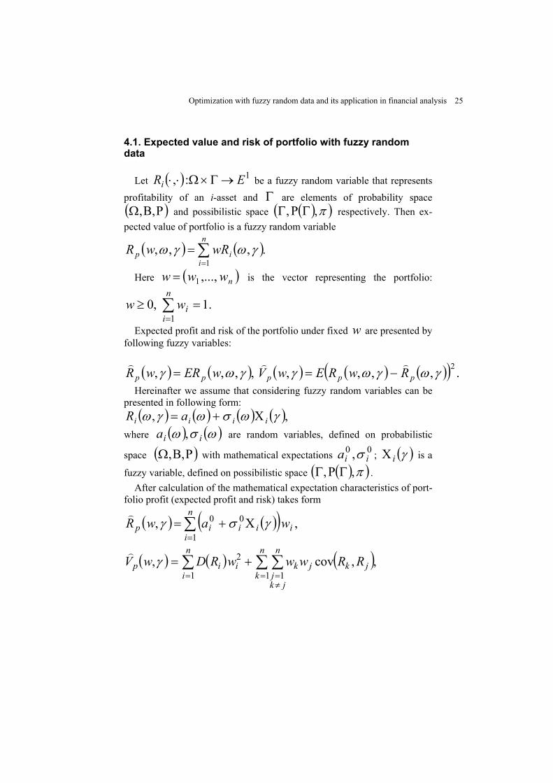
4.1. Expected value and risk of portfolio with fuzzy random data

Let ( ) 1:, ERi →Γ×Ω⋅⋅ be a fuzzy random variable that represents

profitability of an i-asset and Γ are elements of probability space and possibilistic space ( ΒΩ, )Ρ, ( )( )π,, ΓΡΓ respectively. Then ex-

pected value of portfolio is a fuzzy random variable

( ) ( .,,,1∑=

=n

iip wRwR γωγω )

)

Here is the vector representing the portfolio:

∑

( nwww ,...,1=

,=

=n

iiw

1.10≥w

Expected profit and risk of the portfolio under fixed w are presented by following fuzzy variables:

( ) ( ) ( ) ( ) ( )( ) .,,,,,,,, 2γωγωγγωγ ppppp RwREwVwERwR)))

−==

Hereinafter we assume that considering fuzzy random variables can be presented in following form:

( ) ( ) ( ) ( ),, γωσωγω iiii aR Χ+=

where ( ) ( )ωσω iia ,( )ΡΒΩ ,,

are random variables, defined on probabilistic

space with mathematical expectations ; 00 , iia σ ( )γiΧ is a

fuzzy variable, defined on possibilistic space ( )( )π,, ΓΡΓ . After calculation of the mathematical expectation characteristics of port-

folio profit (expected profit and risk) takes form

( ) ( )( ) ,,1

00i

n

iiiip wawR ∑

=Χ+= γσγ

)

( ) ( ) ( ),,cov,1 1

2

1∑ ∑∑=

≠==

+=n

k

n

jkj

jkjki

n

iip RRwwwRDwV γ

)


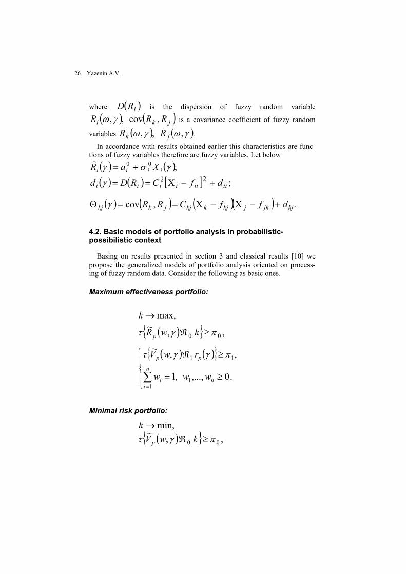
where ( )iRD( )

is the dispersion of fuzzy random variable

( )jki RRR ,, cov,γω is a covariance coefficient of fuzzy random

variables ( ) ( )γωγω ,, jR,kR .

In accordance with results obtained earlier this characteristics are func-tions of fuzzy variables therefore are fuzzy variables. Let below ) ( ) ( );00 γσγ iiii XaR += ( ) ( ) [ ] ;22

iiiiiiii dfCRDd +−Χ==γ

( ) =Θ γkj ( ) ( )( ) .,cov kjjkjkjkkjjk dffCRR +−Χ−Χ=

4.2. Basic models of portfolio analysis in probabilistic-possibilistic context

Basing on results presented in section 3 and classical results [10] we propose the generalized models of portfolio analysis oriented on process-ing of fuzzy random data. Consider the following as basic ones.

Maximum effectiveness portfolio:

max,→k

( ) 00,~ πγτ ≥ℜ kwR p ,

( ) ( )

≥=

≥ℜ

∑=

n

ini

pp

www

rwV

11

11

.0,...,,1

,,~ πγγτ

Minimal risk portfolio:

min,→k ~ ( ) ,, 00 πγτ ≥ℜ kwV p

26 Yazenin A.V.

( ) ( )

≥=

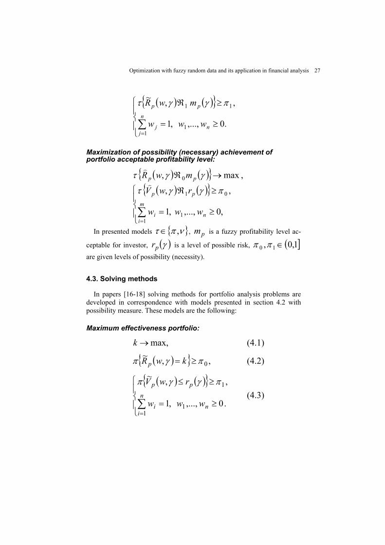
≥ℜ

∑=

n

jnj

pp

www

mwR

11

11

.0,...,,1

,,~ πγγτ

Maximization of possibility (necessary) achievement of portfolio acceptable profitability level:

( ) ( ) max, 0 →ℜ γγτ pp mwR)

, ) ( ) ( )

≥=

≥ℜ

∑=

,0,...,,1

,,

11

01

n

m

ii

pp

www

rwV πγγτ

In presented models νπτ ,∈ , is a fuzzy profitability level ac-

ceptable for investor, pm

( )γpr is a level of possible risk, ( ]1,0, 10 ∈ππ

are given levels of possibility (necessity).

4.3. Solving methods

In papers [16-18] solving methods for portfolio analysis problems are developed in correspondence with models presented in section 4.2 with possibility measure. These models are the following:

Maximum effectiveness portfolio:

max,→k (4.1)

( ) 0,~ πγπ ≥= kwR p , (4.2)

( ) ( )

≥=

≥≤

∑=

n

ini

pp

www

rwV

11

1

.0,...,,1

,,~ πγγπ (4.3)


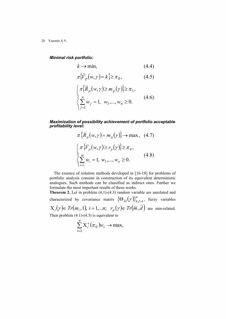
Minimal risk portfolio: min,→k (4.4)

( ) ,,~0πγπ ≥= kwV p (4.5)

( ) ( )

≥=

≥≥

∑=

n

jnj

pp

www

mwR

11

1

.0,...,,1

,,~ πγγπ (4.6)

Maximization of possibility achievement of portfolio acceptable profitability level:

( ) ( ) max, →= γγπ pp mwR)

, (4.7)

( ) ( )

≥=

≥≥

∑=

.0,...,,1

,,

11

0

n

m

ii

pp

www

rwV πγγπ)

(4.8)

The essence of solution methods developed in [16-18] for problems of portfolio analysis consists in construction of its equivalent deterministic analogues. Such methods can be classified as indirect ones. Further we formulate the most important results of these works. Theorem 2. Let in problem (4.1)-(4.3) random variable are unrelated and

characterized by covariance matrix ( ) nlkkl 1, =Θ γ , fuzzy variables

( ) ( ) ;,...1,1, nimTr ii =∈Χ γ ( ) ( )dmTr ,∈γrp are min-related.

Then problem (4.1)-(4.3) is equivalent to

( )∑=

+ →Χn

iii w

10 max,π

28 Yazenin A.V.

( ) ( ) ( )

≥=

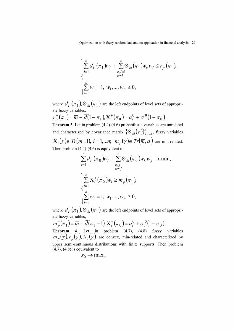
≤Θ+

∑

∑∑

=

+

≠=

−

=

−

,0,...,,1

,

11

111,1

1

n

n

ii

plk

n

lklk

kl

n

iii

www

rwwwd πππ

where ( ) ( 11 , ππ −− Θklid ) are the left endpoints of level sets of appropri-ate fuzzy variables,

( ) ( ) ( ) ( )000

011 1,1 πσπππ −+=Χ−+= ++iiip admr .

Theorem 3. Let in problem (4.4)-(4.6) probabilistic variables are unrelated

and characterized by covariance matrix ( ) nlkkl 1, =Θ γ , fuzzy variables

( ) ( ) ;,...1,1, nimTr ii =∈Χ γ ( ) ( )dmTr ,∈γm p are min-related.

Then problem (4.4)-(4.6) is equivalent to

( ) ( ) min,0,1

0 →Θ+ ∑∑≠

−

=

−jk

n

jkjk

kl

n

iii wwwd ππ

( ) ( )

≥=

≥Χ

∑

∑

=

=

−+

n

ini

n

ipii

www

mw

11

110

,0,...,,1

,ππ

where ( ) ( 11 , ππ −− Θklid ) are the left endpoints of level sets of appropri-ate fuzzy variables,

( ) ( ) ( ) ( )000

011 1,1 πσπππ −+=Χ−+= +−iiip admm .

Theorem 4. Let in problem (4.7), (4.8) fuzzy variables ( ) ( ) ( )γγγ ipp Xrm ,, are convex, min-related and characterized by

upper semi-continuous distributions with finite supports. Then problem (4.7), (4.8) is equivalent to

max0 →x ,


( )( )

( ) ( ) ( )

( ) ( ) ( )

≥=

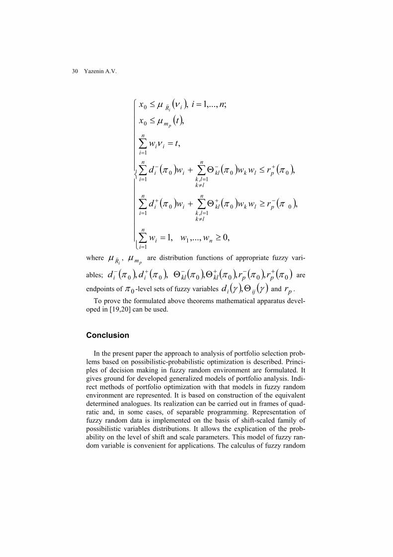
≥Θ+

≤Θ+

=

≤

=≤

∑

∑ ∑

∑ ∑

∑

=

=≠=

−++

=≠=

+−−

=

n

ini

n

i

n

lklk

plkklii

n

i

n

lklk

plkklii

n

iii

m

iR

www

rwwwd

rwwwd

tw

tx

nix

p

i

11

1 1,000

1 1,000

1

0

0

,0,...,,1

,

,

,

,

;,...,1,

πππ

πππ

ν

µ

νµ )

where iR)µ ,

pmµ are distribution functions of appropriate fuzzy vari-

ables; ( ) ( ,0ππ + ),0 id−id ( ) ( ) ( ) ( )0000 ,,, ππππ +−+− ΘΘ ppklkl rr are

endpoints of 0π -level sets of fuzzy variables ( ) ( )γγ ijid Θ, pr and .

To prove the formulated above theorems mathematical apparatus devel-oped in [19,20] can be used.

Conclusion

In the present paper the approach to analysis of portfolio selection prob-lems based on possibilistic-probabilistic optimization is described. Princi-ples of decision making in fuzzy random environment are formulated. It gives ground for developed generalized models of portfolio analysis. Indi-rect methods of portfolio optimization with that models in fuzzy random environment are represented. It is based on construction of the equivalent determined analogues. Its realization can be carried out in frames of quad-ratic and, in some cases, of separable programming. Representation of fuzzy random data is implemented on the basis of shift-scaled family of possibilistic variables distributions. It allows the explication of the prob-ability on the level of shift and scale parameters. This model of fuzzy ran-dom variable is convenient for applications. The calculus of fuzzy random

30 Yazenin A.V.

variables is presented with definition of its moments of the second order in fuzzy form. However, in the frames of proposed schema of possibilistic-probabilistic optimization the models of portfolio analysis and optimiza-tion methods can be developed in case the second order moments of fuzzy random variables are defined in certain form. As a direction of a further re-search a comparative investigation of these two designated approaches and determination of the bounds of its adequate application can be considered.

References

1. S.Nahmias. Fuzzy variables, Fuzzy sets and systems 1(1978) 97-110. 2. S.Nahmias. Fuzzy variables in random environment, In: Gupta M.M. et.

al. (eds.). Advances in fuzzy sets Theory. NHCP. 1979. 3. H.Kwakernaak. Fuzzy random variables – 1.Definitions and theorems,

Inf. Sci.. 15(1978) 1-29. 4. M.D.Puri, D.Ralesky. Fuzzy random variables, J. Math. Anal. Appl.

114(1986) 409-422. 5. A.V.Yazenin, M.Wagenknecht, Possibilistic optimization. Brandenbur-

gische Technische Universitat. Cottbus. Germany. 1996. 6. M.Yu.Khokhlov, A.V.Yazenin. The calculation of numerical character-

istics of fuzzy random data, Vestnik TvGU, No.2. Series «Applied mathematics and cybernetics», 2003, pp.39-43.

7. Y.Feng, L.Hu, H.Shu. The variance and covariance of fuzzy random variables, Fuzzy sets and systems 120(2001) 487-497.

8. A.V.Yazenin. Linear programming with fuzzy random data, Izv. AN SSSR. Tekhn. kibernetika 3(1991) 52-58.

9. A.V.Yazenin. On the method of solving the linear programming prob-lem with fuzzy random data, Izv. RAN, Teoriya i sistemy upravleniya 5(1997) 91-95.

10.H.Markowitz. Portfolio selection: efficient diversification of invest-ments. Wiley. New York, 1959.

11.L.A.Zadeh. Fuzzy sets as a basis for a theory of possibility, Fuzzy sets and systems 1(1978) 3-28.

12.Dubois D., Prade H. Possibility theory: an approach to computerized processing of uncertainty, Plenum press, 1988.

13.M. Inuiguchi, J.Ramik. Possibilistic linear programming: a brief review of fuzzy mathematical programming and a comparison with stochastic programming in portfolio selection problem, Fuzzy sets and systems 111(2000) 3-28.


14.M. Inuiguchi, T.Tanino. Portfolio selection under independent possi-bilistic information, Fuzzy sets and systems 115(2001) 83-92.

15.I.A.Yazenin. Minimal risk and efficiency portfolios for fuzzy random data, XXI Seminar on stability problems of stochastic models. Ab-stracts, Eger, Hungary, 2001, P. 182.

16.I.A.Yazenin, Minimal risk portfolio and maximum effectiveness portfo-lio in fuzzy random environment, Slozhnye sistemy: modelirovanie I optimizatsiya, Tver, TvGU, 2001, pp.59 – 63.

17.I.A.Yazenin, On the methods of investment portfolio optimization in fuzzy random environment, Slozhnye sistemy: modelirovanie I optimi-zatsiya, Tver, TvGU, 2002, pp. 130 – 135.

18.I.A.Yazenin, On the model of investment portfolio optimization, Vest-nik TvGU, No.2. Series «Applied mathematics and cybernetics», 2003, pp. 102 – 105.

19.A.V.Yazenin, On the problem of maximization of attainment of fuzzy goal possibility, Izv. RAN, Teoriya i sistemy upravleniya 4(1999) pp.120 – 123.

20.A.V.Yazenin, On the problem of possibilistic optimization, Fuzzy sets and systems 81(1996) 133-140.

32 Yazenin A.V.

Machine Learning in Fuzzy Environment

Prof., dr.habil.sci.comp. Arkady Borisov Institute of Information Technology Riga Technical University 1 Kalku Street, Riga LV-1658, Latvia E-mail:[email protected] Conditional rule mining (generation) exemplifies one of successful

applications of machine learning. The use of conditional rules is caused by simplicity of input-output relationship description of the task (object) under study. At the same time, the presence of a set of subject area rules is sufficient for solving applied tasks in different areas. First of all, these are tasks of classification (diagnostics), quality control, motion planning, etc.

The main technique of deriving rules of that kind is inductive inference. During the past years a number of effective inductive algorithms were developed. These are, first of all, decision tree generation based rule acquisition techniques suggested in [1,2] as well as the algorithms described in [3,4] that enable one to derive conditional rules escaping the stage of decision tree construction.

One of principal problems in decision tree construction is their size and depth. Major efforts in that area are directed towards obtaining algorithms for constructing trees of a small size that at the same ensure high classification quality. The algorithms differ in computation method of the most informative attribute of the initial data table. Basic methods are entropy measure, information gain, chi-square criterion, GINI index of diversity, gain-ratio, etc.

However, traditional inductive learning methods have proved to be useless for those applied areas that contain vagueness and ambiguity. To cope with that drawback, fuzzy inductive learning algorithms [5] have been developed. They differed in methods of attribute informativeness determination of the initial instance table. One of the first methods suggested were entropy analogue, minimum ambiguity, etc. Besides that, fuzzy rule generation methods were suggested that were directly based on the table of initial fuzzy data [6].

The aforementioned methods have prospects not only in static tasks. Their main task is to serve as self-learning blocks in dynamic conditions.

References

1. Quinlan J.R. (1993). C4.5: Program for Machine Learning, Morgan

Kaufman, San Mateo, CA. 2. Breiman L., Friedman J.H., Olshen R.A., Stone C.J. (1984).

Classification and Regression Tree, Wadsworth International Group, Belmont, CA.

3. Michalski R.S., Chilausky R.L. (1980). Knowledge acquisition by encoding expert rules versus computer induction from examples: a case study involving soybean pathology. International Journal of Man-Machine Studies, N 12, P. 63-87.

4. Clark P., Niblett T. (1989). The CN2 induction algorithm. Machine Learning, 3(4), Kluwer, P.261-283.

5. Yuan Y., Shaw M.J. (1995). Induction of fuzzy decision trees. Fuzzy Sets and Systems, Vol.69, N2, P. 125-139.

6. Ching-Hung Wang, Jau-Fu Liu, Tzung-Pei Hong, Shian-Shyong Tseng. (1999). A fuzzy inductive learning strategy for modular rules. Fuzzy Sets and Systems 103, P. 91-105.

34 Borisov Arkady.

Non-Stochastic-Model Based Finance Engineering

Kaoru Hirota (Tokyo Institute of Technology)

Toshihiro Kaino (Aoyama-Gakuin University) e-mail: [email protected]

Most of the models in the field of finance engineering are proposed based on the stochastic theory, e.g., the well known option pricing model proposed by F. Black and M. Scholes in 1973 is premised on following log normal distribution by the underlying price. Many researchers have also pointed out that this assumption is not always valid for real world financial problems. Although various kinds of improvements have been done, there still exists an application limit with respect to the statistical distribution and the additivity of probability measure, e.g., in evaluation of venture, small, and medium companies, underlying assets are a company and an enterprise, the distribution of the value of underlying assets is not a probability distribution.

A new corporate evaluation model that is able to deal with ambiguous and discrete data better is proposed based on Choquet Integral to overcome the gap mentioned above. First the differentiation of the Choquet integral of a nonnegative measurable function with respect to a fuzzy measure on a fuzzy measure space is proposed and it is applied to the capital investment decision-making problem. Then the differentiation of the Choquet integral of a nonnegative measurable function is extended to differentiation of the Choquet integral of a measurable function, and its properties are shown. The Choquet integral is applied to the long-term debt ratings model, where the input is qualitative and quantitative data of the corporations, and the output is the Moody's long-term debt ratings. The fuzzy measure, that is given as the importance of an each qualitative and quantitative data, is

derived from a neural net method. Moreover, differentiation of the Choquet integral is applied to the long-term debt ratings, where this differentiation indicates how much evaluation of each specification influences to the rating of the corporation.

36 Hirota Kaouru and Kaino Toshihiro

FUZZY DATA MINING IN ECONOMICS AND FINANCE

Plenary Report

Mining Fuzzy Association Rules and Networks in Time Series Databases Batyrshin I., Herrera-Avelar R., Sheremetov L., Suarez R.

Perceptual Time Series Data Mining

A clear view on quality measures for fuzzy association rules De Cock Martine, Cornelis Chris, Kerre Etienne

Moving Approximations in Time Series Data Mining Batyrshin I., Herrera-Avelar R., Sheremetov L., Suarez R.

On Qualitative Description of Time Series Based on Moving Approximations Batyrshin I., Herrera-Avelar R., Sheremetov L., Suarez R.

Generating Fuzzy Rules for Financial Time Series by Neural Networks with Supervised Competitive Learning Techniques

Marček Dušan Pattern Recognition through Perceptually Important Points in Financial Time

Series Zaib Gul, Ahmed Uzair and Ali Arshad

Fuzzy Classification and Pattern Recognition

Soft Clustering for Funds Management Style Analysis: Out-of-sample

Predictability Lajbcygier Paul and Yahya Asjad

Tuning the Fuzzy Classification Models with Various Learning Criteria: the Case of Credit Data Classification

Shtovba Serhiy, Pankevich Olga, and Dounias Georgios prInvestor: Pattern Recognition based Financial Time Series Investment System

Ruta Dymitr On general Scheme of Invariant Clustering Procedures Based on Fuzzy Similarity

Relation Batyrshin I.Z., Rudas T. and Klimova A.

Evolutionary Procedures of Visualization of Multidimensional Data Angelica Klimova

Mining Fuzzy Association Rules and Networks in Time Series Databases

Batyrshin

1,2 I., Herrera-Avelar1 R., Sheremetov1,3 L., Suarez1 R.

1Mexican Petroleum Institute, Mexico 2Institute of Problems of Informatics, Academy of Sciences of Tatarstan, Russia

, [email protected]

Abstract. A new approach to time series data mining (TSDM) is proposed

in this paper. Time series database (TSDB) is considered as a description of dynamics of some system and the goal of TSDM is to find relationships between dynamics of the elements of this system. As such a system it may be considered economic, financial, industrial or natural (Earth Science) systems with the elements described by the sets of time series. The intersystem relationships are formulated as association rules in linguistic form and may be used in perception based reasoning. The general approach to association rules extraction from (crisp) TSDB is based on a consideration of partial (conditional) time series defined in general by perceptual (fuzzy) conditions fulfilled for some time series. Several types of perceptual association rules based on this approach to TSDM are considered in this paper. A new type of association rules based on correlations between partial time series is proposed. These association rules define association network on the elements of the system which may be considered together with spatial, causal, physical etc relations existing in the system. The proposed methods are demonstrated on examples of TSDM in economics and petroleum industry. It is argued that TSDB give regular resources for mining perception based information and for construction, examination and tuning of fuzzy models of knowledge extraction and processing in perception based reasoning.

[email protected]

St. Petersburg Institute for Informatics and AutomationRussian Academy of Sciences (SPIIRAS), Russia

3

1. Introduction

The success of fuzzy logic applications in control, technical systems modeling and pattern recognition is based on synergism of linguistic descriptions and numerical data available for these application areas. Fuzzy logic serves here as a bridge between linguistic and numerical information. One of the reason of the success of fuzzy logic applications in these areas is the existence of regular resources of numerical data obtained from traditional mathematical models, experiments or measurements which can used as a basis for construction, examination and tuning of fuzzy models. In his recent works and lectures Lotfi Zadeh called attention to decision making applications of fuzzy logic in economics, finance, Earth sciences etc. with the central role of human perceptions [13-15]. Perception based propositions like “The price of gas is low and declining”, “It is very unlikely that there will be a significant increase in the price of oil in the near future” etc. are used by peoples in many decision making procedures. Usually perceptions use fuzzy granulation of information obtained from observations, measurements, life experience, mathematical analysis, visual perceptions about curves etc [13, 6]. The formation of perceptions is a process of knowledge extraction from different resources. In this paper we propose the formal methods of extracting such knowledge from time series databases (TSDB). The approach is based on methods developed in data mining [2, 7, 8, 11, 12, 16] for generation of association rules and new methods for generation of crisp and fuzzy association rules from (crisp) TSDB are considered in this paper.

The paper proposes new approach to application of fuzzy logic in economics, finance, medicine, biology, natural and Earth sciences based on analysis of time series data bases existing in these areas. The terabytes of information were collected here during many years and TSDB can give regular and unified resources for fuzzy logic applications in these areas. Linguistic descriptions of patterns of time series like “High value”, “Quickly increasing”, “End of the day”, “Small time period” etc have fuzzy nature and may be described by fuzzy sets defined on the time domain and on the sets of time series values. TSDB can be used also as regular recourses for construction, examination and tuning of perceptual models of knowledge extraction and reasoning.

The concept of association rule is one of the basic concepts of data mining (DM) [2, 11]. One of the well-studied problems in DM is the search for association rules in market basket data. The database in this problem contain records of items bought by customers and the goal of DM is to discover buying patterns of two or more items (e.g. “beer” and “chips”) often bought together.

40 Batyrshin I. et al.

Such patterns are usually represented in the form of association rules like “If beer (is bought) then chips (is bought), (W)” where W is a measure of association between these items usually given by support and confidence measures evaluating how often these items bought together.

In spite of databases (DB) with market basket structure which contain transactions or records with subsets of items the time series data bases (TSDB) contain time series (TS) consisting of sequences of values of some parameter given for increasing time moments. The methods of association rules generation for TSDB usually search the patterns in time series which often followed by other patterns [7, 8].

Two types of TSDB may be differentiated. One type of TSDB contains results of measurement of some parameter or attribute values during given time interval for objects sampled from some population. For example it may be TS of cardiograms measured for the sample of patients, or the TS of annual profit of companies sampled from some sector of economics. Usually in TSDM such type of TSDB is considered and the goal of TSDM consists in extraction of association rules with sequences of patterns often presented in TS, classification of TS (and hence objects) on classes with similar shapes of TS, description of these classes in terms of patterns etc [7, 8, 16]. The methods of solution of such type of problems based on a new technique of moving (sliding) approximations will be considered also in [5]. The traditional problem of TS modeling and forecasting its value also considered in TSDM.

The second type of TSDB which will be considered in this paper contains results of measurements of different parameters measured at the same time moments. We propose a new approach to time series data mining based on consideration of such TSDB as information describing some system of elements evolving in time. As such a system it may be considered the set of countries, regions, industries, companies, petroleum wells etc described by the sets of time series of economical or financial indicators, physical parameters or attributes. Time series data mining (TSDM) is considered in such context as an extraction of information about relationships between elements of this system existing during the evolution of the system. These relationships may be extracted in the form of association rules tying together perceptual patterns of TS for different attributes of the system elements. Such perceptual patterns may be given by crisp or fuzzy granulation of time moments and time series values. Perceptual association rules will define an association network on the set of subsystems which may be considered as information additional to spatial, causal, physical and other relationships existing in the system.

Mining Fuzzy Association Rules and Networks in Time Series Databases 41

If for the first type of TSDB the association rules analyze mainly associations between patterns which often registered together in one time series in neighboring time intervals, for the second type of TSDB the association rules analyze associations between patterns in different time series which happen at the same time intervals. For a mixture of two considered types of TSDB the combination of two types of associations may be studied.

Our approach is based on the analysis of associations between partial or conditional TS given as sets of parts of TS where some condition is fulfilled. The partial TS analysis gives possibility to find associations which are hidden or not clear in the analysis of the entire time series. We demonstrate this approach on the examples of system of economic indicators and system of petroleum wells given by TS of oil and gas production.

The paper is organized as follows. In Section 2 and 3 we consider partial and conditional time series and methods of their definition by simple and composite perceptual patterns (conditions) fulfilled for elements of these time series. In Section 4 we consider the methods of construction of perceptual association rules based on support and confidence measures and demonstrate them on the example of the system of economic indicators. In Section 5 we consider association rules and networks based on partial correlation analysis. In conclusion we discuss the main results and the future directions of the work.

2. Partial time series

Suppose t = (t1, …, tn), (n > 1) is a sequence of time moments such that ti < ti +1 for all t= 1,.., n-1. A time series (TS) y is a sequence of real numbers y = (y1, …, yn) corresponding to the sequence of time moments t. Denote I = (1,…, n) the sequence of indexes of TS. Time series are usually obtained as a result of measurement of some parameter (economical, physical, etc) followed at equal intervals of time. In this case for simplicity it is supposed that t = I = (1,…, n).

A window Wi of a length k 1 is a sequence of indexes Wi= (i, i+1, …, i+k-1), if k > 1, and Wi= (i) if k = 1. Denote ),...,,( 11 −++= kiiiiW yyyy the

corresponding values of TS y in the window Wi. Suppose ),...,( 1 mii WWJ = is a sequence of windows such that i1 <…< im. A sequence ),...,(

1 miWiWJ yyy = will

be called a partial time series (PTS) of y defined by the sequence of windows J. Two special cases of partial time series will be considered. If the lengths of

all windows in J are equal to 1 then J = (i1, …, im), i1 < …< im, and the partial


time series ),...,( 1 miiJ yyy = is a subsequence of TS y. Such partial TS were discussed in [4]. Suppose J = (W1, W2,…, Wn-k+1) is a sequence of all windows of the length k , (1 ≤ k ≤ n). When 1 < k < n the set J contains a set of “moving” or “sliding” windows. Such mowing windows are used in statistics in moving average procedure for smoothing time series when the value in the middle of the window replaced by the mean of values from this window [9]. Moving windows will be considered in data mining procedures based on moving approximations [5]. When k = 1 then J is simply a set of all indexes J = I and when k = n then J contains only one window W1 = I.

Two types of fuzzy partial TS will be considered. Fuzzy set of windows is the sequence of windows Wi accompanied by membership values µi. Set of fuzzy windows J contains fuzzy subsets of I.

A set of elements S = s1,…,sm described by some set of time series will be called a system and his elements will be called subsystems. We will suppose that TSDB contains time series Pi

s=(Pis(t1),…, Pi

s(tn)), obtained as results of measurement of values of parameters (properties, attributes) P = P1,…,Pv for elements s∈S in time moments t= (t1, …, tn). For Pi

s we use also notation Pi(s). For example, S is a system of countries described by time series of economical indicators. Consumer_Price_Index(USA) and Consumer_Price_Index(Mexico) will denote time series of consumer price index values for Mexico and USA. Another example gives a petroleum reservoir with a number of producing wells characterized by time series of oil and gas production during given time period [4], denoted as Oil_Production(Well_N) and Gas_Production(Well_M). The set of all time series describing the subsystems of the system will be denoted as T= x, y, z, …. If each element sk described by only one time series then the set of all TS may be considered as a system. For the set of time series T the sequence of windows J will define the set of partial time series TJ = xJ, yJ, zJ, …. Note that the sets of indexes I and windows J play the role of unified domains for joint analysis of different time series in TSDB describing the given system S.

3. Conditional time series

Suppose a TS y = (y1, …, yn) denotes Pis= (Pi

s(t1),…, Pis(tn)). We will say that

partial time series yJ is defined by condition Pis = A if it consists of all windows

where y satisfies this condition. Such partial time series will be called a conditional time series (CTS). We will consider two types of conditions which will define different types of CTS.


A first type of conditions is fulfilled on the elements of time series and will be called point-wise (pw-) conditions. For example the condition “High price of gas in USA” or Price_of_Gas(USA) = High will define crisp partial TS if High is a crisp interva l [a,b] of gas prices. Then J = j| Pi

s(tj)∈ [a,b], j∈1,…,n, where Pi

s = Price_of_Gas(USA), is the set of time moments when this condition is fulfilled, and corresponding partial TS yJ consists of all elements Pi

s(tj) ∈ [a,b]. If High is defined as a fuzzy interval then J will be a fuzzy subset of I: J= (µj,j)| µj= µHigh(P

is(tj)), j∈1,…,n and yJ = (µj,yj)| µj=

µHigh(Pis(tj)), (j = 1,…,n) will be a fuzzy partial TS. The conditions defined on

time domain will be not related with the elements of system and parameters values but only with time values. For example a condition “End of the day” which may be written as Time = End_of_the_day will define a crisp J = j| tj∈ [a,b], j∈1,…,n or fuzzy J = (µ j,j)| µ j = µEnd of the day (tj), j∈1,…,n sets of indexes if this condition defined as a crisp time interval [a,b] or as a fuzzy set.

The second type of conditions will be called window-wise (ww-) conditions. Windows-wise conditions define a set of windows J where condition is fulfilled. PW-condition may be considered as a special case of ww-condition when the length of window equals to 1. For example ww-condition may be given by “Slowly Increasing price of gas in USA”, describing the property of a

sequence of the values of TS in some window Wj= ))(),...,(),(( 1 kjisj

isj

is tPtPtP ++ .

This condition may be written as Price_of_Gas(USA) = Slowly_Increasing. Explicitation of such conditions also may be crisp or fuzzy. Suppose the following Increasing-Decreasing scale (ID-scale) is used [3]: IDS = QDE:Quickly_decreasing, DEC:Decreasing, SDE:Slowly_decreasing, CON: Constant, SIN: Slowly_increasing, INC: Increasing, QIN: Quickly_increasing. The crisp granulation of the grades of this scale may be done as follows.

Suppose the data in all windows Wj= ))(),...,(),(( 1 kjisj

isj

is tPtPtP ++ from

considered set of windows are approximated by the linear functions yj=pjt+q j. Denote M the maximal absolute slope value from |pj|. The interval Dp= [-dM, dM], where d is a positive constant, e.g. d = 1.2, will be considered as a domain of slope values. The granulation of ID-scale may be obtained as a result of suitable partition of Dp on intervals. For example, if Dp = [-10,10], then the crisp granulation of ID-scale may the following: QDE=[-10,-7]; DEC=[-7,-4]; SDE=[-4,-1]; CON=[-1,1]; SIN= [1,4]; INC=[4,7]; QIN=[7,10]. As a result, the numerical slope value pj of linear function approximating TS data in window Wj can be retranslated into corresponding linguistic grade of ID-scale.


Windows-wise property may be given also by conditions defined on a time domain Dt like “During the year”. Depending on the meaning of this condition Dt will be partitioned on the time intervals corresponding to calendar years or the set of sliding windows with the length of 365 days will be defined.

A fuzzy ww-conditions will define a fuzzy set of windows or a set of fuzzy windows. For example if the granulation of ID-scale considered above is given by fuzzy intervals [3] defined on Dp then the numerical slope value pj of linear function yj=pjt+qj approximating TS data in window Wj will belong to fuzzy grade SIN: Slowly_increasing with some membership value µj and the fuzzy condition Price_of_Gas(USA) = Slowly_Increasing will define the fuzzy set of windows (µj,Wj) where µj may be considered as a degree of fulfillment of this condition on the window Wj. A fuzzy condition “During a small time period” will define a sliding set of fuzzy windows defined on time domain. Example of association rules for ww-conditions will be considered further.

The third type of conditions will be called external conditions. It is related with the properties of subsystems described by TS. If a subsystem satisfies to this property with some degree a, then we will suppose that all elements of time series related with this subsystem satisfy to this property with the same degree µ(i) = a, (i=1,…,n). For example if TS describes the sale volumes of some article during one year then the properties like “Expensive article” or “High quality article” will be external for this TS.

The condition defining the set of windows J and corresponding conditional time series may be simple like conditions considered above or composite one obtained as a result of logical combination of simple conditions. For example the conditions P = “The high level of oil production in well number 1 in winter months” and Q = “Quick increase of price on oil or low level of currency reserve” may be written as P = (P1 AND P2) and Q = (Q1 OR Q2) where P1: “Level_of_oil_production(Well_1) = High”, P2:“Time= Winter_month”, Q1:“Oil_Price= Quick_increase”, Q2 = “Level_of_ currency_ reserve= Low”. Linguistic connectives AND and OR will define corresponding (fuzzy) set theoretic operations on the set of (fuzzy) windows .

4. Association rules with support and confidence measures

The basic framework of the association rule mining in DB is formalized as follows [2,11,12]. Let I = i1, i2,.., im be a set of distinct literals called items


and D = T1, T2, . . . , Tn be a database of transactions or baskets of items such that Ti ⊆ I. In general, associa tion rules have the form A ⇒ B or

R: If A then B, (W), (1)

where A ⊂ I, B ⊂ I and A ∩B = ∅. For market basket data, for example, A and B denote some groups of items bought together. For evaluating significance, informative usefulness or strength of the association between A and B some measures W like support and confidence are used. Support and confidence measures are defined as follows:

supp(R) = D

BA ∩, conf(R)=

A

BA ∩,

(2)

where |A∩B| is the number of transactions containing items A and B together and |D| is a total number of transactions in database D. In some approaches instead of intersection A∩B of sets A and B it is used union A∪B. Association rules usually do not causal but associative, i.e. B takes place together which A but may be not caused by A. Additionally to these measures some measures for selecting of informative rules are used [11,12]. J-measure is defined as follows:

¬¬

¬+=)(

)/(log)/(

)()/(

log)/()();(BP

ABPABP

BP

ABPABPAPABJ ,

(3)

where P(A) is a probability of the set of items A in D, etc. The extension of association rules and association measures on time series

databases may be done as follows. Suppose A and B are crisp point-wise conditions (simple or composite) and JA and JB are the corresponding sets of indexes. Support and confidence measure will be defined as follows:

supp(R) = N

JJ BA ∩, conf(R)=

A

BA

J

JJ ∩,

(4)

where N = n is a number of time moments. If A and B define fuzzy sets of indexes JA and JB then fuzzy cardinality is used in (4):

supp(R) = ∑ ∧=

N

iBA ii

N 1))()((

1µµ , conf(R)=

∑

∑ ∧

=

=N

iA

N

iBA

i

ii

1

1

)(

))()((

µ

µµ.

(5)


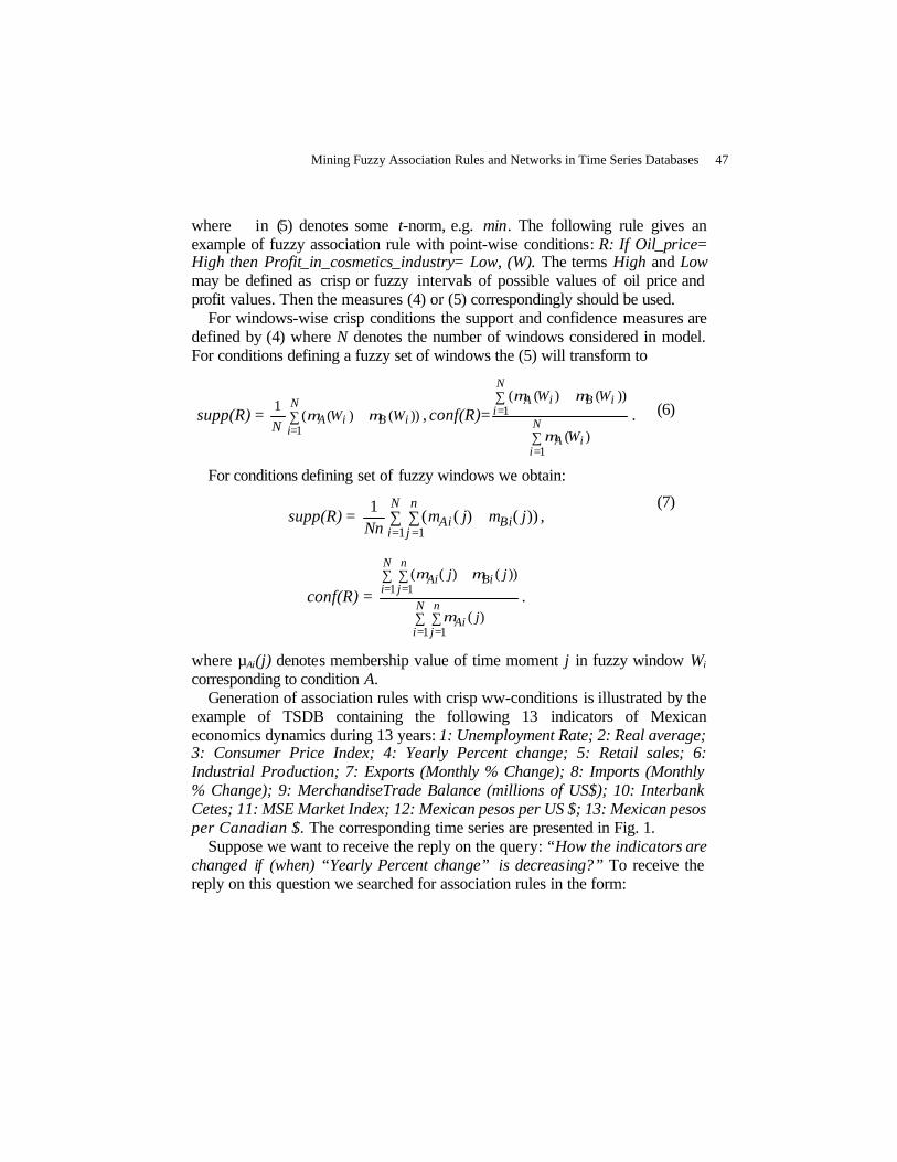
where ∧ in (5) denotes some t-norm, e.g. min. The following rule gives an example of fuzzy association rule with point-wise conditions: R: If Oil_price= High then Profit_in_cosmetics_industry= Low, (W). The terms High and Low may be defined as crisp or fuzzy intervals of possible values of oil price and profit values. Then the measures (4) or (5) correspondingly should be used.

For windows-wise crisp conditions the support and confidence measures are defined by (4) where N denotes the number of windows considered in model. For conditions defining a fuzzy set of windows the (5) will transform to

supp(R) = ∑ ∧=

N

iiBiA WW

N 1))()((

1µµ , conf(R)=

∑

∑ ∧

=

=N

iiA

N

iiBiA

W

WW

1

1

)(

))()((

µ

µµ.

(6)

For conditions defining set of fuzzy windows we obtain:

supp(R) = ∑ ∑ ∧= =

N

i

n

jBiAi jj

Nn 1 1))()((

1 µµ ,

conf(R) = ∑ ∑

∑ ∑ ∧

= =

= =N

i

n

jAi

N

i

n

jBiAi

j

jj

1 1

1 1

)(

))()((

µ

µµ

.

(7)

where µAi(j) denotes membership value of time moment j in fuzzy window Wi corresponding to condition A.

Generation of association rules with crisp ww-conditions is illustrated by the example of TSDB containing the following 13 indicators of Mexican economics dynamics during 13 years: 1: Unemployment Rate; 2: Real average; 3: Consumer Price Index; 4: Yearly Percent change; 5: Retail sales; 6: Industrial Production; 7: Exports (Monthly % Change); 8: Imports (Monthly % Change); 9: MerchandiseTrade Balance (millions of US$); 10: Interbank Cetes; 11: MSE Market Index; 12: Mexican pesos per US $; 13: Mexican pesos per Canadian $. The corresponding time series are presented in Fig. 1.

Suppose we want to receive the reply on the query: “How the indicators are changed if (when) “Yearly Percent change” is decreasing?” To receive the reply on this question we searched for association rules in the form:


If Yearly_Percent_change = Decreasing then K = Decreasing, (8)

If Yearly_Percent_change = Decreasing then K = Increasing, (9)

where K denotes indicators different from “Yearly Percent change”.

05

1 01

05

1 02

05

1 03

05

1 04

05

1 05

05

1 06

05

1 07

05

1 08

05

1 09

05

1 01 0

05

1 01 1

05

1 01 2

2 4 6 8 1 0 1 205

1 01 3

Fig. 1. Time series of 13 indicators of Mexican economics

For finding such association rules we considered all set of windows of size 2 such that the total number of windows equals to N = 12. For each window Wi=(i,i+1) the value of considered indicator K is determined by the values yi of indicator as follows: K = Increasing, if yi+1 > yi, and K = Decreasing, if yi+1 < yi. The similar approaches to evaluating ID-value considered also in [1,3]. The set JA in (4) is a set of windows Wi where the condition Yearly_Percent_change = Decreasing is fulfilled. The set JB in (4) is a set of windows Wi where the


condition K = Decreasing is fulfilled. The calculation of support and confidence measures was done for rules (8), (9) for all indicators K different from “Yearly Percent change” and the rules with confidence and support values greater than 0.5 were selected as more valuable. As result three rules of type (8) for indicators K= 3, 10, 12, and one rule of type (9) for indicator K = 11 were selected. The confidence and support values were equal (c= 0.75, s= 0.5) for these rules with K= 3, K= 10 and K= 11, and (c= 0.875, s= 0.583) for the rule with K= 12. But a calculation of the measure of informative value (3) for these rules give the maximal value for rules with indicators K= 3 and K= 11. Finally the following two most informative rules were obtained:

If Yearly_Percent_change = Decreasing then Consumer_Price_Index = Decreasing,

If Yearly_Percent_change = Decreasing then MSE_Market_Index = Increasing.

It should be noted that the rule (8) with indicator K= 12: “Mexican pesos per US” received the maximal values of confidence and support and almost the minimal value of J-measure in comparison with other rules. It may be explained by the fact that this indicator is decreasing in almost all windows.

The use of Increasing-Decreasing scale considered in Section 3 gives possibility to receive more fine crisp or fuzzy rules like If Yearly_Percent_change= Quickly_Decreasing_then K = Slowly_Increasing. Generally more complex patterns of TS like convex-concave patterns [6] may be considered.

5. Association rules based on correlation measure

In [4] it was proposed the method of generation of rules like

R: If A(si) then P(sj) associated with Q(sk), (W), (10)

where A(si) is a condition fulfilled for subsystem si and P(sj), Q(sk) are some parameters evaluated for subsystems sj, sk. The following is an example of such association rule:

R: If Oil_production(Well_T101)= High then Oil_production(Well_T25)

highly associated with Gas_production(Well_T03),(W),


where High represented generally by a crisp or fuzzy interval of oil production values. Then the condition of rule will define a crisp or fuzzy set of indexes J.

Suppose the condition A(si) in (10) defines the crisp set of indexes J, and x, y are time series corresponding to P(sj) and Q(sk). As a measure of association between P(sj) and Q(sk) a correlation [9,16] of PTS xJ and yJ was considered:

−∑

−−

=∈ Jy

Ji

Ji Jx

JiJJ

yyxx

Jyxr

σσ11

),( (11)

where ∑=∈Ji

iJ zJ

z1 , ( )∑ −

−=

∈JiiJz zz

J

2

11

σ , for z = x or z = y. The

association between xJ and yJ is considered as high if t-test [9] shows high level of significance of this association, where t calculated as follows:

)1()2( 2rJrt −−= . (12)

Here r is a correlation coefficient and |J|-2 is called a degree of freedom. The set of association rules which may be generated for the condition A(si)

defines some weighted relation on the set of time series and subsystems and considered as an association network defined on the set of subsystems. This association network may be combined and compared with other relations existing between subsystems, such as spatial relations, causal relations etc and will give additional information about the structure of the considered system.

This approach was applied to association network construction for the system of 4 wells T03, T25, T43, T101 from a Mexican reservoir based on the analysis of partial time series of oil and gas production in these wells registered during several years. For example, the following two association rules with high significance value were generated for condition Oil_production(Well_T43)= High:

R: If Oil_production(Well_T43)= High then Oil_production(Well_T25) highly associated with Oil_production(Well_T03),

R: If Oil_production(Well_T43)= High then Oil_production(Well_T25) highly associated with Oil_production(Well_T101).

The analysis of association networks obtained for different conditions showed high association between T3 well oil production and T25 well oil and gas production. After comparison of association networks with spatial location of wells in reservoir this fact obtained a natural explanation since T3 well is located above T25 well and not far from it. But association between these wells


was not evident before this analysis because, actually, T3 well belongs to another rock formation than the wells T25, T43 and T101. This analysis showed also that the pairs of wells with similar distances between them have different pair wise associations. This fact gives possibility to raise hypothesis about heterogeneity of rock properties in reservoir.

The proposed approach may be extended on the case of fuzzy conditions. Suppose condition A(si) in (10) defines fuzzy set of indexes J. Define the sequence of levels L=a1< a2<… < ac, ak ∈[0,1] and corresponding sequence of a-cuts of fuzzy set J: J1⊇ J2⊇… ⊇ Jc. For each level set Jk we calculate correlation rk by (11) and corresponding value of t by (12). Denote R = rk. Applying extension principle of Zadeh we determine a fuzzy subset of correlation values on the set R as follows: k

rkrar

== max)(µ . Degree of freedom

of correlation value r from R is obtained by extension principle of Zadeh as follows: 2max −=

=k

rkrr JN which will define by t-test a significance of

corresponding association. The extension principle may be applied also to the levels of significance of t-test. Fuzzy correlations are considered also in [10].

Conclusions

In this paper, a novel data mining approach for generation of fuzzy and crisp association rules from (crisp) TSDB based on partial time series analysis is proposed. Partial time series given by crisp or fuzzy conditions are determined by the sets of crisp or fuzzy windows where this condition is fulfilled. The methods of calculation of confidence and support measures for new type of association rules are proposed in the paper. The efficiency of this measure was illustrated by the example of analysis of TSDB describing the dynamic of the system of economical parameters of Mexico.

A new type of association rules based on partial correlation measure considered also in the paper. The approach is illustrated using an example of the time series of petroleum wells oil and gas production from a Mexican reservoir. The initial correlations (obtained in a classical way) between time series did not show high associations between production volumes of the analyzed wells. However, the analysis of the partial time series gave the possibility to find such associations. These associations were described by rules and presented as association networks in 3D representation of wells in reservoir. Later on, these association networks gave the possibility to compare


the obtained associations with the geophysical information and other reservoir properties. Such analysis offers the possibility of better understanding of the existing relationships in analyzed system of wells which are hidden or not clear enough before this analysis. The possible generalization of this approach on fuzzy partial correlation analysis is discussed.

Industrial and economic systems are often characterized by the sets of time series describing the change in time of economical, financial or technological parameters. The analysis of associations between these TS, e.g. in macro economical analysis, can give the possibility to understand the relationships between subsystems of the system and their subsystems, which may be represented in linguistic or graphic form and used in perceptual decision making system or in informal analysis. Being a bridge between linguistic and numerical information, fuzzy logic gives us the tools for description and extraction of knowledge in crisp TSDB and for the further use of this knowledge in perception based reasoning. Generally the algorithms of generation of association rules in large DB require a lot of operations and one of the main problems in DM is development of algorithms with minimal complexity. This problem exists also in fuzzy TSDM but the main advantage of the perception based queries to TSDB is that they can essentially decrease the complexity of the algorithms decreasing the search space. TSDB form an efficient environment for construction, examination and tuning of fuzzy perceptual models.

Acknowledgements

The support for this research work has been provided by the IMP, projects D.00006 “Distributed Intelligent Computing”.

References

[1] Alvarez-Ramirez J, Soriano A, Cisneros M, Suarez R (2003) Symmetry/ anti-symmetry phase transitions in crude oil markets. Physica A: Statistical Mechanics and its Applications, vol. 322(C), pp. 583-596

[2] Agrawal R, Imelinski T, Swani A (1993) Mining association rules between sets of items in large database. In Proc. ACM SIGMOD Int. Conf. Management of Data, pp. 207-216

[3] Batyrshin I (2002) “On granular derivatives and the solution of a granular initial value problem,” Int. J. Appl. Math. Comp. Sci. (Special Issue on Computing with


Words and Perceptions, D. Rutkowska, J. Kacprzyk and L.A. Zadeh, Eds.) vol. 12, pp. 403 – 410. (http://matwbn.icm.edu.pl/ksiazki/amc/amc12/amc1236.pdf)

[4] Batyrshin I, Cosultchi A, Herrera -Avelar R (2004) Association Network of Petroleum Wells Based on Partial Time Series Analysis. Proc. Workshop on Intelligent Computing. (Ed. by L. Sheremetov and M. Alvarado), Mexico City, Mexico, pp. 17 – 26

[5] Batyrshin I, Herrera -Avelar R, Sheremetov L, Suarez R (2004) Moving Approximations in Time Series Data Mining. FSSCEF 2004, (in this volume)

[6] Batyrshin I, Panova A (2003) “On convex-concave perception based functions,” in Proceedings of EUSFLAT 2003, Zittau, Germany, pp. 485– 490

[7] Das G, Lin KI, Mannila H, Renganathan G, Smyth P (1998) Rule Discovery from Time Series. KDD, pp. 16-22

[8] Last, M, Klein Y, Kandel A (2001) Knowledge Discovery in Time Series Databases. IEEE Transactions on Systems, Man, and Cybernetics, vol. 31B, pp. 160-169

[9] Lindgren BW (1998) Statistical Theory (Fourth Edition). Chapman-Hall [10] Pedrycz W, Smith MH (1999) Granular correlation analysis in Data Mining. Proc.

IEEE Int. Fuzzy Systems Conf. Korea, pp. III-1235 – III-1240 [11] Piatetsky-Shapiro G (1991) Discovery, analysis and presentation of strong rules.

In Piatetsky-Shapiro G., and Frawley W.J. eds. Knowledge Discovery in Databases. Menlo Park, CA: AAAI Press. pp. 229-248

[12] Smyth P, Goodman RM (1992) An information theoretic approach to rule induction from databases. IEEE Trans. Knowledge Data Engineering 4, vol. 4, pp. 301-316

[13] Zadeh LA (1997) Toward a theory of fuzzy information granulation and its centrality in human reasoning and fuzzy logic, Fuzzy Sets and Systems, vol. 90, pp. 111-127

[14] Zadeh LA (1999) From computing with numbers to computing with words - from manipulation of measurements to manipulation of perceptions, IEEE Trans. on Circuits and Systems - 1: Fundamental Theory and Applications, vol. 45, pp. 105-119

[15] Zadeh LA (2001) A New Direction in AI: Toward a Computational Theory of Perceptions, AI Magazine, Spring 2001 issue.

[16] Zhang P, Huang Y, Shekhar S, Kumar V (2003) Correlation analysis of spatial time series datasets: a filter-and-refine approach. In: Proc. PAKDD '03, Lecture Notes in AI. Vol. 2637, Springer-Verlag, Seoul, Korea, pp. 532-544


A Clear View on Quality Measures for FuzzyAssociation Rules

Martine De Cock, Chris Cornelis, and Etienne E. Kerre

Fuzziness and Uncertainty Modelling Research UnitDepartment of Applied Mathematics and Computer ScienceGhent University, Krijgslaan 281 (S9), 9000 Gent, Belgiumtel: +32 9 2644742, fax: +32 9 2644995, http://fuzzy.UGent.beMartine.DeCock, Chris.Cornelis, [email protected]

1 Introduction

In today’s information—driven economy, companies may benefit a lot from suit-able knowledge management. Although knowledge management is not just atechnology—based concept but rather a business practice in general, the pos-sible and even indispensable support of IT—tools in this context is obvious.Because of the large data repositories many firms maintain nowadays, an im-portant role is played by data mining techniques that dig up useful knowledgefrom these large data volumes. Among them, association rules [1] provide aconvenient and effective way to identify and represent certain dependenciesbetween attributes in a database. Originally, association rules emerged in thedomain of shops and customers; the basic idea is to identify frequent itemsetsin market baskets, i.e. groups of products frequently bought together. Store-keepers may use this information to decide on how to place merchandise onshelves to maximize a cross—selling effect, how to advertise, what to put onsale (for instance lowering the price of product A to attract customers, mean-while increasing the price of product B that is frequently bought togetherwith A), . . . Evidently, the application of association rules can shed light ona wide range of decision making and marketing problems going beyond thescope of straightforward storekeeping.

Association rule mining is traditionally performed on a data table withbinary attributes. Conceptually, a record x in the data table represents acustomer transaction, whereas the attributes represent items that may beeither purchased in that transaction, or not. Therefore, for each attributeA, A(x) is either 1 or 0 indicating whether or not item A was bought intransaction x. An association rule is an expression of the form A ⇒ B inwhich A and B are attributes, such as cheese ⇒ bread. The meaning is thatwhen A is bought in a transaction, B is likely to be bought as well.

In most real life applications, databases contain many other attribute val-ues besides 0 and 1. Very common for instance are quantitative attributes suchas age or income, taking values from a partially ordered, numerical scale, oftena subset of the real numbers. One way of dealing with a quantitative attributelike cost is to replace it by a few other attributes that form a crisp partitionof the range of the original one, such as low = [0, 100[, medium = [100, 300[and high = [300,+∞[. Now we can consider these new attributes as binaryones that have value 1 if the cost attribute equals a value within their range,and 0 otherwise. In this way, the problem is reduced to the mining proceduredescribed above [9]. From an intuitive viewpoint, it makes more sense howeverto draw values from the interval [0, 1] (instead of just 0, 1), to allow recordsto exhibit a given attribute to a certain extent only. In this way binary at-tributes are replaced by fuzzy ones. The corresponding mining process yieldsfuzzy association rules (see e.g. [2, 4, 5, 6, 7]).

Association rules can be rated by a number of quality measures, amongwhich support and con¯dence stand out as the two essential ones. Supportmeasures the statistical significance of a candidate rule A⇒ B, whereas con-fidence assesses its strength. The basic problem of mining association rules isthen to generate all association rules A⇒ B that have support and confidencegreater than user—specified thresholds. These measures can be generalized forfuzzy association rules in several ways.

The goal of this paper is not to introduce yet another series of quality mea-sures, but to shine a bright light on what has been proposed so far. Section2 deals with the first pillar of our argument: the identification of transactionsin a database as positive or negative examples of an association between at-tributes. Along the way we recall the basic concepts of support and confidence,initially in the framework of crisp association rules. Soon however we move onto the mining of fuzzy association rules as it is specifically in this setting thatnew and seemingly aberrant quality measures have been proposed recently,such as non—symmetrical measures of support. The second important pillar inthis paper is that support and confidence measures should actually be thoughtof as compatibility and inclusion measures respectively (Section 3). Leaningon both pillars, in Section 4 we take the mystery out of some recently pro-posed quality measures for fuzzy association rules by providing clear insightinto their true semantics.

2 Positive and Negative Examples

2.1 Crisp Association Rules

Let X be a non—empty data table containing records described by their valuesfor binary attributes A belonging to a set A. For an attribute A and a recordx ∈ X, A(x) = 1 means item A was purchased in transaction x, while A(x) = 0means A was not bought. In this way, A can also be thought of as the set

A clear view on quality measures for fuzzy association rules 55

of transactions containing the item, i.e. x ∈ A iff A(x) = 1, and x /∈ A iffA(x) = 0. Likewise coA is the set of transactions not containing the item,i.e. x ∈ coA iff A(x) = 0, and x /∈ coA iff A(x) = 1. Let A,B ∈ A. Thesupport of an association rule A⇒ B is usually defined as

supp(A⇒ B) = |A ∩B|/|X | (1)

i.e. the number of elements belonging to both A and B, scaled to a valuebetween 0 and 1. The idea behind the definition of support is to measurethe statistical significance by counting positive examples, i.e. transactions thatexplicitly support the hypothesis expressed by the association rule. It is worthnoting that the positive examples of A⇒ B are also those of the rule B ⇒ A,i.e. support is a symmetric measure. Hence, as can be expected, it only revealspart of the global picture. This is why we also need the confidence measure,to assess the strength of a rule. Traditionally, if a rule A ⇒ B generates asupport exceeding a user—specified threshold, it is meaningful to compute itsconfidence, i.e. the proportion of correct applications of the rule.

conf(A⇒ B) = |A ∩ B|/|A| (2)

Note that |A| will not be 0 if we assume that the confidence is computed onlywhen the support exceeds a certain threshold (which should be greater than0 to be meaningful).

Having identified the “supporters” of A⇒ B as positive examples, we canask ourselves what a negative example of the same rule might look like. It isclear that a transaction violates the rule A⇒ B as soon as it contains A butnot B. As opposed to positive examples, a negative example of A ⇒ B isno negative example of B ⇒ A, and vice versa. Also, the complement of theset of positive examples does not necessarily equal that of negative examples,just like a “non—negative example” differs from a “positive example”. This issummarized in Table 1 (see also [4]). It is interesting that Dubois et al. [5]

Table 1. The nature of transaction x w.r.t. rules A⇒ B and B ⇒ A

x A⇒ B B ⇒ Apositive example x ∈ A ∧ x ∈ B x ∈ A ∧ x ∈ B

non-positive example x /∈ A ∨ x /∈ B x /∈ A ∨ x /∈ Bnegative example x ∈ A ∧ x /∈ B x /∈ A ∧ x ∈ B

non-negative example x /∈ A ∨ x ∈ B x ∈ A ∨ x /∈ B

also distinguish between positive and negative examples that are grouped intosets they call S+ and S− respectively. Furthermore, they introduce the class ofirrelevant examples S± as S± = x ∈ X | x ∈ A. One can easily verify thatour classes of non—positive and non—negative examples are obtained as unions

56 De Cock Martine, Cornelis Chris. and Kerre Etienne

of S± with the set of positive and negative examples, respectively. Also, whileS−, S+ and S± form a partition of X, this is clearly not the case for the fourclasses we defined. The most important reason we choose to consider them isthat they all give rise to different measures:Definition 1. The quality measures M1 ,M2 ,M3 , and M4 of the rule A⇒ Bare respectively defined as

M1(A⇒ B) = |A ∩ B|/|X| M3(A⇒ B) = |A ∩ coB|/|X|

M2(A⇒ B) = |coA ∪ coB|/|X| M4(A⇒ B) = |coA ∪ B|/|X|

It can be easily verified thatM2(A⇒ B) = 1−M1(A⇒ B) and M3(A⇒ B) = 1−M4(A⇒ B) (3)

Hence, only two measures are independent. We can for instance choose towork with M1 and M4 . The measure M1 corresponds to the symmetrical sup-port measure (supp) of Formula (1), while M4 is a non—symmetrical measuretaking into account all examples that do not violate the rule A⇒ B.

2.2 Fuzzy Association Rules

Recall that a fuzzy set A inX is anX → [0, 1] mapping. Fuzzy—set—theoreticalcounterparts of complementation, intersection, and union are defined, as usual,by means of a negator, a t-norm, and a t-conorm. Recall that an increasing,associative and commutative [0, 1]2 → [0, 1] mapping is called a t-norm Tif it satisfies T (x, 1) = x for all x in [0, 1], and a t-conorm S if it satisfiesS(x, 0) = x for all x in [0, 1]. A negator N is a decreasing [0, 1] → [0, 1]mapping satisfying N (0) = 1 and N (1) = 0. For A and B fuzzy sets in X wedefine coNA(x) = N (A(x)), A ∩T B(x) = T (A(x), B(x)), and A ∪S B(x) =S(A(x), B(x)) for all x in X .

Let A(x) be the degree to which an attribute A is bought in a transactionx (or in a broader context: the degree to which x satisfies the attribute). Thisway A can be thought of as a fuzzy set in the universe of transactions, and themeasures discussed above have to be generalized accordingly. The cardinalityof a fuzzy set in a finite universe X is defined as usual as the sum of theindividual membership degrees. Replacing the set—theoretical operations inDefinition 1 by their fuzzy—set—theoretical counterparts (defined by means ofa negator N , a t-norm T , and a t-conorm S), we obtainDefinition 2. The quality measures M1 ,M2 ,M3 , and M4 of the rule A⇒ Bare respectively defined asM1(A⇒ B) = 1

|X|∑x∈X

(A ∩T B)(x) M3(A⇒ B) = 1|X|

∑x∈X

(A ∩T coNB)(x)

M2(A⇒ B) = 1|X|

∑x∈X

(coNA ∪S coNB)(x) M4(A⇒ B) = 1|X|

∑x∈X

(coNA ∪S B)(x)


The natural extension of Formula (3) holds when N is the standard negatorNs (defined by Ns(x) = 1−x for all x in [0, 1]) and (T ,S,Ns) is a de Morgantriplet, i.e. T (x, y) = Ns(S(Ns(x),Ns(y))) for all x and y in [0, 1]. Generalizingthe confidence measure listed above to the fuzzy case, the following formulais obtained:

conf(A⇒ B) =

∑x∈X

(A ∩T B)(x)∑x∈X

A(x) (4)

3 Inclusion and Compatibility of Fuzzy Sets

Typically, to define fuzzy subsethood one takes a definition of classical setinclusion and tries to extend (“fuzzify”) it to apply to fuzzy sets. Below wequote three distinct, but essentially equivalent1 , definitions of the inclusion ofA into B, where A and B are crisp subsets of X:

A ⊆ B ⇐⇒ (∀x ∈ X)(x ∈ A⇒ x ∈ B), (5)

⇐⇒ A = ∅ or | A ∩ B || A | = 1, (6)

⇐⇒ | coA ∪B || X | = 1 (7)

While (5) is stated in strictly logical terms, the other two are based on countingthe elements of a set, i.e. on cardinality, and have a probabilistic (i.e. frequen-tist) flavour. It is therefore not surprising that their respective generalizationsto fuzzy set theory cease to be equivalent and give rise to cardinality—basedand logical inclusion measures, respectively [3]. For instance, formula (5) canbe generalized to fuzzy sets by replacing the two—valued implication by a[0, 1]—valued implicator. Recall that an implicator I is a [0, 1]2 → [0, 1] map-ping such that I(x, .) is increasing and I(., x) is decreasing, and I(1, x) = xfor all x in [0, 1], and I(0, 0) = 1. An inclusion measure satisfying desirableproperties is then given by

Inc1(A,B) = infx∈X

I(A(x), B(x))

However this approach has certain disadvantages in applications. Indeed, iftwo fuzzy sets A and B are equal everywhere, except in the point x for whichA(x) = 1 and B(x) = 0, then Inc1(A,B) = 0. One can think of very concreteinstances in which this indeed makes no sense. Imagine for instance that we areto evaluate to what extent the young people in a company are also rich. Testingsubsethood of the fuzzy set of young workers into that of rich workers shouldthen be based on the relative fraction (i.e. the frequency) of good earners1 Arguably, (5) is more general since it can also deal with infinite sets.


among the youngsters, and not on whether there exists or does not existone poor, young employee. This observation has led researchers to considerextensions to definition (6) of crisp subsethood. If A and B are fuzzy sets,then one can define the subsethood of A into B as

Inc2(A,B) =|A ∩T B||A|

if A = ∅, and 1 otherwise.In formula (7) the presence of implication is also very clear. For proposi-

tions p and q in binary logic, p ⇒ q has the same truth value as ¬p ∨ q. Thecounterpart in fuzzy logic is the so-called S—implicator induced by S and N ,defined by IS,N (x, y) = S(N (x), y) for all x and y in [0, 1]. Generalizing for-mula (7) hence gives rise to a softened version of Inc1 in which the supremumis replaced by taking the average over all elements of X :

Inc3(A,B) =1|X |

∑

x∈XIS,N (A(x), B(x))

Another well-studied class of implicators are the residual implicators IT , in-duced by a t-norm T in the following way: IT (x, y) = supλ|λ ∈ [0, 1] andT (x,λ) y for all x and y in [0, 1].

Another important kind of comparison measures for fuzzy sets, the so—called compatibility measures, assess their degree of overlap (see e.g. [10]).The so—called simple matching coefficient

Com1(A,B) =|A ∩T B||X | = 1

|X |∑

x∈XT (A(x), B(x))

is the average degree to which the fuzzy sets A and B together span theuniverse X. It is a softened version of

Com2(A,B) = supx∈X

T (A(x), B(x))

which is the height of the T —intersection of fuzzy sets A and B. Compatibilitymeasures are symmetrical but in general not reflexive.

4 A Clear View on the Semantics of the Measures

Throughout the literature on fuzzy association rules, the quality measureslisted in Table 2 are prominent. The first and the third measure are generallyaccepted as measures of support and confidence respectively. They assess thesignificance and the strength of a fuzzy association rule. They coincide witha compatibility measure (Com1) and an inclusion measure (Inc2) from fuzzyset theory.


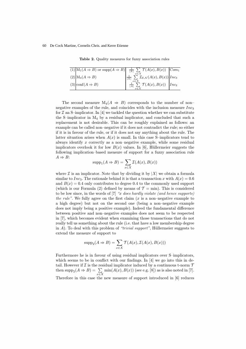
Table 2. Quality measures for fuzzy association rules

(1) M1(A⇒ B) or supp(A⇒ B) 1|X|

∑x∈X

T (A(x), B(x)) Com1

(2) M4(A⇒ B) 1|X|

∑x∈X

IS;N (A(x), B(x)) Inc3

(3) conf(A⇒ B) 1|A|

∑x∈X

T (A(x), B(x)) Inc2

The second measure M4(A ⇒ B) corresponds to the number of non—negative examples of the rule, and coincides with the inclusion measure Inc3for I an S—implicator. In [4] we tackled the question whether we can substitutethe S—implicator in M4 by a residual implicator, and concluded that such areplacement is not desirable. This can be roughly explained as follows: anexample can be called non—negative if it does not contradict the rule; so eitherif it is in favour of the rule, or if it does not say anything about the rule. Thelatter situation arises when A(x) is small. In this case S—implicators tend toalways identify x correctly as a non—negative example, while some residualimplicators overlook it for low B(x) values. In [6], Hullermeier suggests thefollowing implication—based measure of support for a fuzzy association ruleA⇒ B:

supp1(A⇒ B) =∑

x∈XI(A(x), B(x))

where I is an implicator. Note that by dividing it by |X | we obtain a formulasimilar to Inc3. The rationale behind it is that a transaction x with A(x) = 0.6and B(x) = 0.4 only contributes to degree 0.4 to the commonly used support(which is our Formula (2) defined by means of T = min). This is consideredto be low since, in the words of [7] \x does hardly violate (and hence supports)the rule". We fully agree on the first claim (x is a non—negative example toa high degree) but not on the second one (being a non—negative exampledoes not imply being a positive example). Indeed the fundamental differencebetween positive and non—negative examples does not seem to be respectedin [7], which becomes evident when examining those transactions that do notreally tell us something about the rule (i.e. that have a low membership degreein A). To deal with this problem of \trivial support", Hullermeier suggests toextend the measure of support to

supp2(A⇒ B) =∑

x∈XT (A(x), I(A(x), B(x)))

Furthermore he is in favour of using residual implicators over S—implicators,which seems to be in conflict with our findings. In [4] we go into this in de-tail. However if I is the residual implicator induced by a continuous t-norm Tthen supp2(A⇒ B) =

∑x∈X

min(A(x), B(x)) (see e.g. [8]) as is also noted in [7].

Therefore in this case the new measure of support introduced in [6] reduces


to the commonly used one, and hence does not offer anything new. For thisreason we disagree with the claim of [5] that whereas the traditional supportmeasure (i.e. supp or M1) is in line with the conjunction—based approach tomodelling fuzzy rules, the above—defined measure supp2 follows the traditionof implication—based fuzzy rules. Within the literature on fuzzy associationrules there exists another view on the use of Inc3 as well. Chen et al. [2] callthis measure “degree of implication” and use it to replace the traditional con-fidence measure. This should not come as a great surprise, since their relianceon Inc3 yields just another way of expressing the subsethood of A into B. Forthis reason we also prefer to view the non—symmetrical measure M4 as a confi-dence measure. Finally, since association rule mining is concerned with findingfrequent patterns in databases, it seems more natural to use cardinality—basedrather than logical compatibility and inclusion measures, which explains whyInc1 and Com2 are not met in literature on fuzzy association rules.

Acknowledgements The results presented in this paper were obtainedwithin the bilateral China—Flanders cooperation project 174B0201. MartineDe Cock and Chris Cornelis would like to thank the Fund for Scientific Re-search Flanders—FWO for funding the research reported in this paper.

References1. Agrawal R, Imielinski T, Swami A (1993) Mining Association Rules betweenSets of Items in Large Databases. Proceedings of ACM SIGMOD conference onManagement of Data, 207—216

2. Chen G, Yan P, Kerre E E (2004) Computationally Efficient Mining for FuzzyImplication—based Association Rules in Quantitative Databases. To appear in:International Journal of General Systems

3. Cornelis C, Kerre E E (2003) Inclusion Measures in Intuitionistic Fuzzy SetTheory. Lecture Notes in Computer Science 2711:345—356

4. De Cock M, Cornelis C, Kerre E E (2003) Fuzzy Association Rules: a Two-SidedApproach. Proceedings of FIP2003, 385—390

5. Dubois D, Hullermeier E, Prade H (2003) A Note on Quality Measures forFuzzy Association Rules. Lecture Notes in Computer Science 2715:346—353

6. Hullermeier E (2001) Fuzzy Association Rules: Semantic Issues and QualityMeasures. Lecture Notes in Computer Science 2206:380—391

7. Hullermeier E (2002) Mining Implication-Based Fuzzy Association Rules inDatabases. Proceedings of IPMU2002, Vol. I:101—108

8. Novak V, Perfilieva I, Mockor J (1999) Mathematical Principles of Fuzzy Logic.Kluwer

9. Srikant R, Agrawal R (1996) Mining Quantitative Association Rules in LargeRelational Tables. Proceedings of ACM SIGMOD Conference on Managementof Data, v.25 n.2:1—12

10. Tsiporkova E, Zimmermann H-J (1998) Aggregation of Compatibility andEquality: a New Class of Similarity Measures for Fuzzy Sets. Proceedings ofIPMU1998, 1769—1776


Moving Approximations in Time Series Data Mining

Batyrshin1,2 I., Herrera-Avelar1 R., Sheremetov1 L., Suarez1 R.

1Mexican Petroleum Institute, Mexico 2Institute of Problems of Informatics, Academy of Sciences of Tatarstan, Russia [email protected]

Abstract. In this paper we propose a new technique for time series (TS) analysis called moving approximations. It defines a new procedure of TS transformation called Moving Approximations Transform (MAPT). Based on this transformation of TS two new measures of association between TS are introduced: a measure of local trend associations and a measure of local trend distances. The properties of invariance of MAPT and association measures to linear transformations of TS are studied. An example of association analysis of the set of TS from economics is described. As result of such analysis the association network and classification of TS is obtained.

1. Introduction

Time series data mining (TSDM) is actively developed research area [6, 7]. Traditional approaches to time series (TS) analysis study the problems of time series modelling and forecasting its values [5]. TSDM consider such problems as association rules extraction from TS data bases (TSDB), search of patterns in TS, TS classification, piece-wise linear representation (PLR), linguistic summarization of TS etc. [4, 6-9, 12]. Such technique like Fourier and Wavelet transforms are very important tools in TS analysis and TSDM [4,8].

In this paper we propose new approach to TSDM which use analysis of local trends in TS. This approach is based on the concepts of partial time series analysis when the parts of two time series are compared and on consideration

of TSDB as a description of the dynamics of the system [2]. In such contexts TSDM consists in analysis of local associations between dynamics of TS describing elements of the system. Local dynamic of TS maybe described by terms like “increasing”, “decreasing”, “constant” which may be evaluated by the slope value of linear regression of TS on considered segment. The comparison of such slope values for two TS on the same segments gives possibility to analyze associations between the changes of these TS. In this paper we consider a sequence of moving windows like in moving average procedure used for TS analysis and extract slope values of linear approximations of TD values on these windows. Moving approximations transform (MAPT) replace the sequence of TS values by the sequence of slope values. Based on MAPT new association measures are introduced. This measures may be used for construction of association network on the set of TS and for classification of TS on the classes of highly associated TS. The distance measure between slope values for short TS and TS classification based on this measure is considered also in [9].

The paper is organized as follows. In Section 2 MAPT is introduced and studied. In Section 3 new measures of TS association based on MAPT are introduced and studied. An example of application of these measures to analysis associations between TS in economics is considered in Section 4. In Conclusion main results and future work is discussed.

2. Moving approximations transform

Suppose t = (t1, …, tn), (n > 1) is a sequence of time moments such that ti < ti +1 for all t= 1,.., n-1. A time series (y,t) is a sequence of real numbers y = (y1, …, yn) corresponding to the sequence of time moments t. Denote I = (1,…, n) the sequence of indexes of time series (TS). Time series are usually obtained as a result of measurement of some parameter (economical, physical, etc) followed at equal intervals of time.

A window Wi of a length k > 1 is a sequence of indexes Wi= (i, i+1,…, i+k-1). Denote ),...,,( 11 −++= kiiiiW yyyy the corresponding values of TS y in the

window Wi. Suppose ),...,( 1 mii WWJ = is a sequence of windows such that

i1<…< im. A sequence ),...,(1 miWiWJ yyy = will be called a partial time series

Moving Approximations in Time Series Data Mining 63

of y defined by the sequence of windows J. A sequence of all windows of the length k , J = (W1, W2,…, Wn-k+1), (1 < k ≤ n), will be called a moving (or sliding) windows. We will denote it also as Jk and the set of indexes of all windows in Jk as Ik = (1,2,…, n-k+1). Such mowing windows are used in statistics in moving average procedure for smoothing time series when the value in the middle of the window replaced by the mean of values from this window [5]. The set of all time series in TSDB will be denoted as T = x, y, z, …. For the set of time series T the sequence of windows J will define the set of partial time series TJ = xJ, yJ, zJ, …. Here the sets of windows J plays the role of unified domain for joint analysis of different time series in TSDB describing the given system S.

Suppose J = (W1, W2,…, Wn-k+1) are moving windows Wi= (i, i+1, …, i+k-1) of size k and ),...,,( 11 −++= kiiiiW yyyy , i∈ Ik = (1,2,…, n-k+1) are

corresponding partial time series. A linear functions fi = ait+bi with parameters ai,bi minimizing the criterion

( ) ( )∑ −+=∑ −=−+

=

−+

=

1 21 2)(),(ki

ijjiji

ki

ijjjiiWi ybtaytfyfQ , (1)

will be called a moving least squares approximation of yWi. The parameters ai, bi of moving least squares approximations can de calculated as follows:

∑ −

∑ −−

=−+

=

−+

=1 2

1

)(

))((

ki

ijij

ki

ijijij

itt

yytt

a , iiii tayb −= ,

where ∑=−+

=

11 ki

ijji t

kt , ∑=

−+

=

11 ki

ijji y

ky ,

(2)

Definition 1. Suppose a = (a1, …, an-k+1) is a sequence of slope values

obtained as a result of moving approximations of time series (y,t) in moving windows of size k. A transformation MAPk(y,t)= a will be called a moving approximation transform (MAPT) of time series y.

The slope values a= (a1, …, an-k+1) will be called local trends.


Suppose p,q,r,s are real values, r ≠ 0 and y, z are time series given in the same time moments t = (t1, …, tn). Denote py+q = (py1+q, …, pyn+q) and y+z= (y1+z1, …, yn+zn).

Proposition 2. A MAPT satisfies for all real values p,q,r,s, (r≠ 0), and time series z the following properties:

1) MAPk(py+q,t)= pMAPk(y,t); 2) MAPk (y,rt+s)= (1/r)MAPk (y,t); 3) MAPk (y+z,t)= MAPk (y,t) + MAPk (z,t).

Corollary 3. MAPT is invariant to equal simultaneous linear transformations of time values and time series values, i.e.

MAPk (ry+s,rt+s)= MAPk (y,t). Corollary 4. Suppose time moments t = (t1, …, tn) are increasing with a

constant step h such that ti+1 - ti = h for all i = 1,…, n-1. Then in MAPT the set of time moments t = (t1, …, tn) can be replaced by the set of indexes I = (1,…, n) as follows:

MAPk (y,t) = (1/h)MAPk (y,I). Corollary 5. Suppose mean(y1,…, ym) = (mean(y1

1,…, y1m),…,

mean(yn1,…, yn

m)) is a mean value of m time series calculated element-wise in time moments t=(t1,…, tn), then mean(MAPk(y

1,t),…, MAPk(ym,t))=

MAPk(mean(y1,…, ym), t). From Proposition 2 it follows also: MAPk(-y,t)= - MAPk(y,t). Further we will replace time series by corresponding MAP transform.

Considered above properties show how the operations on time series can be replaced by corresponding operations on their MAPT. Because the conditions of the Corollary 4 as usually are fulfilled for time series we will suppose that t = I = (1,…, n) if time moments are not mentioned and use notation MAPk(y). Also, if the size of windows in moving approximations does not important or fixed we will write simply MAP(y).

3. New measures of time series association based on local trend analysis

Our goal is to introduce the measure of association between time series which could evaluate the relationships between the changes in time of time series describing the system evolution during considered time period. We say that y is


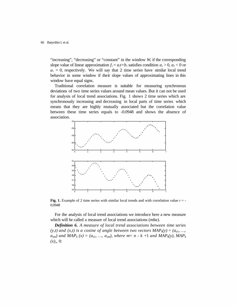
“increasing”, “decreasing” or “constant” in the window Wi if the corresponding slope value of linear approximation fi = ait+bi satisfies condition ai > 0, ai < 0 or ai = 0, respectively. We will say that 2 time series have similar local trend behavior in some window if their slope values of approximating lines in this window have equal signs.

Traditional correlation measure is suitable for measuring synchronous deviations of two time series values around mean values. But it can not be used for analysis of local trend associations. Fig. 1 shows 2 time series which are synchronously increasing and decreasing in local parts of time series which means that they are highly mutually associated but the correlation value between these time series equals to -0.0948 and shows the absence of association.

0 1 2 3 4 5 6 7-62

-60

-58

-56

-54

0 1 2 3 4 5 6 755

56

57

58

59

60

61

Fig. 1. Example of 2 time series with similar local trends and with correlation value r = -0.0948

For the analysis of local trend associations we introduce here a new measure which will be called a measure of local trend associations (mlta).

Definition 6. A measure of local trend associations between time series (y,t) and (x,t) is a cosine of angle between two vectors MAPk(y) = (ay1, …, aym) and MAPk (x) = (ax1, …, axm), where m= n - k +1 and MAPk(y), MAPk (x)≠ 0:


∑⋅∑

∑ ⋅==

==

=m

jxj

m

iyi

m

ixiyi

kkk

aa

aaxMAPyMAPxymlta

1

2

1

2

1))(),(cos(),( ,

(3)

From the definition the properties of this measure are following: mltak(y, x)=mltak (x,y); -1 ≤ mltak (y, x) ≤ 1; mltak (y, y) = 1; mltak (y, -y) = -1; mltak (y, -x) = -mltak (y, x); mltak (-y, -x) = mltak (y, x).

Generally, for two given time series the measure of local trend associations defines a sequence of association values (mlta2,…, mltan) depending on the size of windows. The selection of the size of the moving windows will define the level of detailing of the analysis of associations between time series. In the presence of random fluctuations in time series values the size of windows k should not be very small. For time series presented in Fig. 1 the value of this measure equal to 0.923 for moving approximations with window size equal to 5. The high value of mlta reflects the fact that these time series are highly associated due to synchronous increase and decrease in local parts of TS.

Suppose p,q,r,s are real constants and p,r ≠ 0. A time series (z,u) obtained as a result of a linear transformation of time series (y,t), such that zi = pyi+q and ui = rti+s, i = 1,…, n will be denoted as (z,u) = L(y,t).

Proposition 7. Suppose (x,t) and (y,t) are two time series and L1 and L2 are two linear transformations of time series given by the sets of parameters (p1,q1,r1,s1) and (p2,q2,r2,s2) respectively, then

mltak(L1(x,t), L2(y,t)) = sign(p1)⋅sign(r1)⋅sign(p2)⋅sign(r2)⋅mltak((x,t), (y,t)). Theorem 8. A measure |mlta| is invariant to linear transformations of

time series. Theorem 8 shows very nice property of introduced association measure. It

means particularly that time series may be normalized independently and the absolute measure of local trend associations |mlta| will be not changed.

Definition 9. A measure of local trend distances between time series (y,t) and (x,t) is defined as an Euclidean distance between two vectors MAPk(y)

= (ay1, …, aym) and MAPk(x)= (ax1, …, axm), (m= n - k +1):


∑ −===

m

ixiyikkk aaxMAPyMAPdxymltd

1

2)())(),((),( , (4)

From the definition it follows the metric properties of mltd: mltdk(y, x)=mltdk (x,y); mltdk (y, x) 0 and mltdk (y, x) = 0 if and only if y=x; mltak (y, x) ≤ mltak (y, z) + mltak (z, x).

Proposition 10. Suppose p,q,r,s, (r ≠ 0), are real values and (z,t) is a time series. A measure of local trend distances satisfies for all time series (y,t) and (x,t) the following properties:

mltdk(y+q, x+s) = mltdk(y, x); mltdk(y+z, x+z) = mltdk(y, x); mltdk(py, px) = p⋅mltdk (y, x);

These introduced measures were tested on many artificial and real examples of time series and showed very good results. Examples of application of this measure to generation of association networks of real time series of economical data are considered in the following section.

4. Example of association analysis

The proposed approach to local trend analysis was applied to analysis associations between 10 time series of gross internal product in Mexico checked quarterly during the period 1980 – 2003 [1]. Each time series contains 96 data. The mlta3 measure with windows size equal to 3 was used for calculation pair-wise associations between time series. Fig. 2 shows association networks constructed sequentially for different levels of |mlta| values such that on each level only associations with the value greater than this level are shown.


-10 0 10

-10

-5

0

5

10

1

2

34

5

6

7

8 9

10

level = 0.89

-10 0 10

-10

-5

0

5

10

1

2

34

5

6

7

8 9

10

level = 0.81

-10 0 10

-10

-5

0

5

10

1

2

34

5

6

7

8 9

10

level = 0.72

-10 0 10

-10

-5

0

5

10

1

2

34

5

6

7

8 9

10

level = 0.6

-10 0 10

-10

-5

0

5

10

1

2

34

5

6

7

8 9

10

level = 0.55

-10 0 10

-10

-5

0

5

10

1

2

34

5

6

7

8 9

10

level = 0.52

Fig. 2. Association networks with different levels of association

Below are the classes of time series obtained as sets of nodes of connected subgraphs shown in Fig. 2.

C1. 5: Electricity, Gas and Water; 9: Social and Personal Communal Services; 1: Farming, Forestry and Fishes;

C2. 8: Financial Services, Insurance, Real Estate Activities and Rent; 10: Liability to Banking Services Allocate;

C3. 3: Manufacturing Industry; 4: Construction; 6: Commerce, Restaurants and Hotels;

C4. 2: Mining; C5. 7: Transport, Storage and Communications. On more low levels time series number 2 have more associations with the

class C3 and time series 7 with the class C2.


Fig. 3. Time series grouped in correspondence with the obtained

classification. The number of time series is shown on its right side. Evidently, the obtained classes have good interpretation and the time series

from these classes shown in Fig. 3 have the similar shapes. The TS in Fig. 3 grouped in correspondence with obtained classifications.

Conclusion

The paper introduces a new technique for time series (TS) analysis based on moving approximation transform. In MAPT time series replaced by the


10 20 30 40 50 60 70 80 900

50100

2

10 20 30 40 50 60 70 80 900

50100

3

10 20 30 40 50 60 70 80 900

50100

4

10 20 30 40 50 60 70 80 900

50100

6

10 20 30 40 50 60 70 80 900

50100

5

10 20 30 40 50 60 70 80 900

50100

9

10 20 30 40 50 60 70 80 900

50100

1

10 20 30 40 50 60 70 80 900

50100

7

10 20 30 40 50 60 70 80 900

50100

8

10 20 30 40 50 60 70 80 900

50100

sequence of slopes of approximating lines. Such MART representation of TS gives possibility to introduce measures of local trend associations and distances which gives possibility to analyze and compare local dynamic of TS. The approach is demonstrated on the example of association analysis and classification of TS of economical data.

The developed technique of local trend analysis gives possibility to introduce perceptive fuzzy granulation [3,10,11] of the set of slope values and generate linguistic descriptions like “slowly increasing”, “quickly decreasing” etc. The rules and descriptions of such type may be used further for perception based reasoning about systems described by the set of time series. The methods of generation of such type of rules are considered in [3].

Acknowledgements


References

[1] Banco de Información Económica http://dgcnesyp.inegi.gob.mx/bdine/bancos.htm

[2] Batyrshin I., Herrera-Avelar R, Sheremetov L, Suarez R (2004) Mining Fuzzy Association Rules and Networks in Time Series Databases. International Conference on Fuzzy Sets and Soft Computing in Economics and Finance, FSSCEF 2004, St. Petersburg, Russia, 2004 (in this volume).

[3] Batyrshin I, Herrera-Avelar R, Sheremetov L, Suarez R (2004) On Qualitative Description of Time Series Based on Moving Approximations. International Conference on Fuzzy Sets and Soft Computing in Economics and Finance, FSSCEF 2004, St. Petersburg, Russia, 2004 (in this volume).

[4] Boyd S (1998) TREND: a system for generating intelligent descriptions of time-series data. In Proceedings of the IEEE International Conference on Intelligent Processing Systems (ICIPS-1998).

[5] Brockwell PJ, Davis RA, Fienberg SE (1991) Time Series: Theory and Methods (Springer Series in Statistics) February, 1991.

[6] Keogh E, Kasetty S (2002) On the Need for Time Series Data Mining Benchmarks: A Survey and Empirical Demonstration. In SIGKDD ’02, Ju1y, 23-26 2002


[7] Last M, Klein Y, Kandel A (2001) Knowledge Discovery in Time Series Databases. in IEEE Transactions on Systems, Man, and Cybernetics Vol. 31B.

[8] Mörchen F (2003) Time series feature extraction for data mining using DWT and DFT. Data Bionics, Philipps-University Marburg, Hans-Meerwein-Strasse, 35032 Marburg, Germany, October 9, 2003.

[9] Möller-Levet CS, Klawonn F, Cho KH, Wolkenhauer O (2003) Fuzzy Clustering of Short Time-Series and Unevenly Distributed Sampling Points. IDA 2003 pp. 330-340.

[10] Zadeh LA (1997) Toward a theory of fuzzy information granulation and its centrality in human reasoning and fuzzy logic. Fuzzy Sets and Systems, vol. 90, pp. 111-127.

[11] Zadeh LA (1999) From computing with numbers to computing with words - from manipulation of measurements to manipulation of perceptions,” IEEE Trans. on Circuits and Systems - 1: Fundamental Theory and Applications, vol. 45, pp. 105-119.

[12] Zhang P, Huang Y, Shekhar S, Kumar V (2003) Correlation analysis of spatial time series datasets: a filter-and-refine approach. In the Proc. Seventh Pacific-Asia Conf. Knowledge Discovery Data Mining, (PAKDD '03), Lecture Notes in Artificial Intelligence Vol. 2637, Springer-Verlag, Apr. 30-May 2, Seoul, Korea pp. 532-544


On Qualitative Description of Time Series Based on Moving Approximations

Batyrshin1,2 I., Herrera-Avelar1 R., Sheremetov1 L., Suarez1 R.

1Mexican Petroleum Institute, Mexico 2Institute of Problems of Informatics, Academy of Sciences of Tatarstan, Russia batyr,herrerar,sher, [email protected]

Abstract. In this paper we propose a new method of piece-wise linear representation (PLR) of time series. Such representation is based on a moving approximations transform (MAPT) of time series in the sequence of local slope values. PLR is based on granulation of the set of slope values and on the sequential merging and splitting of segments of TS. Resulting PLR is retranslated in the form of rules containing linguistic terms like “quickly increasing”, “slowly decreasing” etc. The possible applications of PLR and rule based representation of TS in classification of TS and in perceptive reasoning are discussed.

1. Introduction

Time series (TS) are important sources for decision making in business and in science. The problem of qualitative analysis of TS arises in such areas like data mining, process monitoring, diagnosis and control, reasoning about processes, etc. The qualitative analysis of TS is related with coding, compressing, classification and search TS in databases, search of valuable patterns in data, linguistic description for knowledge extraction, inductive generalization, perceptive reasoning and decision making in knowledge based systems [1-3, 5-9]. The importance of development of such methods is increasing with the exponential growth of the size of TS databases in finance, economics, medicine, manufacturing, science, geophysics, technology etc. used in research and decision making procedures.

Piecewise linear representation (PLR) of time series gives possibility to reduce the complexity of TS data, describe them qualitatively as a sequence of straight lines, generate linguistic descriptions etc [2, 5 – 7, 9].

In this paper a new method of adaptive piece-wise linear representation of time series based on MAP transform [1] of TS is proposed. This method is based on scaling of slope values of linear segments which gives possibility to retranslate them in perceptive evaluations like “Quickly increasing”, “Slowly decreasing” etc. The method described in Section 2. His work is demonstrated in Section 3 on 2 examples of real time series from economics. In Conclusion the obtained results are discussed.

2. Adaptive PLR of Time Series Based on MAPT

Our goal is to transform PLR of TS in rules

Rk: If X is Tk then Y is Sk, (1)

where Tk is a linguistic term like LESS THAN 5, GRATER THAN 40, BETWEEN 10 AND 15 describing some (may be fuzzy) interval Ak [2]. The Sk is a linguistic term like DECREASING, CONSTANT and QUICKLY INCREASING, which describes the speed of function’s y change on Ak. The rule set (1) will give qualitative description of given TS. Term Sk will code the slope pk of the function yk = pkx + qk that approximates the data yi on Ak.

We will suppose that on a set of possible slope values P a scale Lp= P1,…, PM, (Pj∈P) such that Pj < Pj+1 for all j = 1,…, M-1 is defined. This numerical scale defines a linguistic scale Ls= s1,…, sM+1 with linguistic terms such that for each numerical slope value p, a corresponding linguistic term from Ls may be pointed out as follows: S(p) = s1, if p≤ P1, S(p) = sj, if Pj-1 < p ≤ Pj, for j=2,…, M and S(p)= sM+1, if PM < p. It should be noted that the scale of numerical slope values Lp is usually context dependent because the slope values may vary for different TS. In these cases different numerical scales of slope values may be used. But linguistic scale Ls as usually context insensitive and depends only on the number of grades in the scale Lp. For example, for different sets of TS two different numerical scales may be obtained: Lp = -5, -3, -1, 1, 3, 5 and Lp = -0.07, -0.04, -0.01, 0.01, 0.04, 0.07 but in both cases for coding the numerical slope values, the same linguistic scale may be used:

Ls= QDC:Quickly Decreasing, DEC:Decreasing, SDC:Slowly Decreasing,

CON: Constant, SIN: Slowly Increasing, INC: Increasing, QIN: Quickly Increasing .


The essential part of our PLR algorithm is the use of linguistic scales. The adaptive PLR of TS algorithm consists in the following steps: MAP transform of TS with small windows, linguistic coding of slopes obtained by MAPT, merging windows with similar slopes and finally separate intersected windows on non-intersected windows, which finally will give PLR of TS. Here we use some ideas for merging segments from [2]. But instead of initial partition on small intervals we use initial cover of points by windows obtained in MAPT. The idea of the proposed method is to transform the system of highly intersected windows in the set of non-intersected segments (windows) by merging and splitting segments obtained from initially constructed windows.

The general scheme of proposed procedure consists of the following six steps.

1. Apply Moving Approximations Transform. MAPT generates windows (segments) Gi= (i,…, i+D-1), (i= 1,…, n-D+1) with D points. Each segment approximated by linear function yi=pix+q i and TS replaced by the sequence of slopes (p1,…,pn-D+1). Determine the codes S(pi) of slope values for all segments.

2. Join similar segments. Compare the slope codes of each two neighboring segments starting from the first segment. If some pair of segments has equal slope codes, join them in a new segment. Calculate a linear approximation and correspondent linguistic slope code for the new segment. Repeat this step while the neighboring segments with equal slope codes exist.

3. Delete covered segments. Denote Q the set of all segments and R an empty set: R= ∅. Find in Q a segment Gi with maximum number of points. Sequentially delete from Q segments Gi+k, (k=1,…), if all points of them covered by Gi and Gi+k+1, i.e. if Gi+k ⊆ Gi ∪ Gi+k+1. Similarly delete all segments Gi-k, (k=1,…), if all points of them are covered by Gi and Gi-k-1. Delete segment Gi from Q and write it in R. Repeat this procedure till Q is empty. Rewrite all segments from R in Q. After each deleting of covered segment join similar segments.

4. Delete segments with small uncovered sub-segments. For each segment determine the set of points which do not belong to neighboring segments. This set is called an uncovered sub-segment (USS). Determine the size of all USS. While small USS with the size less than given threshold H exists, use one of the following transformations of segments. Denote the segment with small USS as Gs and his left and right neighboring segments as Gl and Gr respectively. Check the following two possibilities.

P1. Delete Gs and add its uncovered points to Gl and Gr such that the total error of linear approximations of all points of new two segments E2 is minimum. Resulting two new segments are non-intersected.

On Qualitative Description of Time Series Based on Moving Approximations 75

P2. Suppose all points of three segments Gs, Gl and Gr may be divided in three new non-intersected segments Gs

*, Gl* and Gr

* such that Gs

* ⊆ Gs, Gl* ⊆

Gl and Gr*

⊆ Gr and the size of each new segment is greater or equal than H. Construct such three non-intersected segments which minimize the total error E3 of linear approximation of all points of Gs, Gl and Gr.

If E2 ≤ E3 then build new two segments by P1, otherwise build new three segments by P2. After obtaining new segments join similar segments.

5. Separate intersected segments. If after application of all previous steps some two segments are still intersected then disjoint the points from this intersection between these segments such that the total error of linear approximations of new two non-intersected segments will be minimal. After obtaining new segments join similar segments.

6. Retranslate the obtained PLR. The obtained PLR of data on non-intersected segments G1,…, Gm is fully represented by the set of parameters (xk1, xk2, pk, qk), (k=1,…,m), where xk1 and xk2 are the first and the last points of Gk and pk, qk are parameters of linear function yk = pkx+qk approximating data from Gk. The rule (1) may be in the simplest case constructed as follows:

Rk: If X is BETWEEN xk1 and xk2 then Y is S(pk). (2)

Often, in qualitative description of data exact values of xk1 and xk2 are not meaningful and may be replaced by nearest values of some grid defined on X [2]. For example, if values of X denote weights in kilograms but qualitative descriptions operate by tons then exact values xk1 and xk2 will be rounded till some new numbers Xk1 and Xk2 and (2) will be transformed in the form:

Rk: If X is BETWEEN Xk1 and Xk2 then Y is S(pk) (3)

The meaning of intervals BETWEEN Xk1 and Xk2 in rule base (3) is fuzzy because they denote some uncertain set of crisp intervals “similar” to these intervals. Moreover, these fuzzy intervals may be further generalized and replaced by fuzzy terms like SMALL WEIGHT, END OF THE DAY, HIGH etc. Such hierarchical fuzzy granulation of values of parameters is typical for qualitative descriptions [2]. The qualitative generalization of obtained PLR of TS may be used for further aggregation of rules in more general and compact form and for inference of conclusions about dependencies. For example, the qualitative evaluation of width and localization of segments may be used in perception based decision-making procedure based on generalized rule base.

Contrary, when the information about segments does not important in qualitative description of TS then the set of rules (1) may be written in simplified form as the sequence of linguistic labels of slopes (S1, …, Sm) from


consequent parts of rules or by the sequence of slope values (p1,…, pm) of. Such coding of TS may be considered as generalized MAP transform of TS and used in further TSDM.

3. Examples of PLR of TS

The proposed MAR-PLR procedure depends on a set of following parameters: the size of window, the size H of minimal uncovered segment and the scale Lp of slope values. The variation of these parameters gives possibility to analyze possible structures of TS. MAR-PLR showed good results on a large set of both artificial and real data downloaded from INTERNET. For example, on artificial data from [2], MAR-PLR shows the same results but works more quickly than evolutionary algorithm considered in [2]. Below we discuss the results of application of MAR-PLR on two TS downloaded from INTERNET.

First TS contains information about Industrial Production Index published by Board of Governors of the Federal Reserve System [4]. It includes monthly data of time period from 1940-01-01 to 2003-07-01. Data are presented on the upper part of Fig. 1.

Fig. 1. Industrial Production Index.


We used the numerical slope scale: -250, -150, -50, 50, 150, 250 corresponding to linguistic scale Ls considered in Section 2. The size of windows equals 30 months and size of minimal segment equals to 24 months. The piece-wise linear representation of data obtained by MAR-PLR is presented on the upper and separately on the lower part of Fig. 1. The following sequence of slope values were obtained: (217.1, -281.0, 81.2, 174.1, 296.9, -94.2, 117.0, 346.1, 22.7, 416.8, -75.5). The retranslation of these slope values gives the following sequence of linguistic codes: (INC, QDC, SIN, INC, QIN, SDC, SIN, QIN, CON, QIN, SDC). The last two rules have the form:

R10: If X is BETWEEN year 1993 and year 2000 then Y is Quickly

Increasing, R11: If X is BETWEEN year 2000 and year 2003 then Y is Slowly

Decreasing.

As a result of qualitative analysis it may be further concluded that “During last 2,5 years the Index Slowly Decreased, whereas during 8 years before, it Quickly Increased”. Qualitative description of this TS may be used also for finding association between this TS and other TS in TS database.

Fig. 2 shows results of PLR of data of Civilian Unemployment Rate monthly evaluated during time period 1948-01-01 to 2003-07-01 and published by the U.S. Department of Labor [10]. As it may be seen from Fig. 2, MAP can build good enough PLR of TS with sufficiently complex shapes.

Conclusions

The new method of qualitative description of time series is developed. It builds piece-wise linear representation of time series and transforms it in the rule set which may be used in perceptive decision making procedures [2, 11, 12]. Other positive features of the proposed procedure are the adaptive selection of the number of segments used for PLR and the use of numerical and linguistic scales of slope values for qualitative granulation of the speed of the function change. The first feature is overcome some known methods of PLR of TS which require a priory definition of the number of segments. The use of the scales of slope values gives possibility to change the qualitative description of data depending on the context of the problem and translate them in context insensitive perceptive linguistic descriptions. The proposed method based on


moving approximations transform [1] is faster than the similar method based on evolutionary generated fuzzy partitions [2].

Fig. 2. Civilian Unemployment Rate.

Acknowledgements


References

[1] Batyrshin I, Herrera-Avelar R, Sheremetov L, Suarez R (2004) Moving Approximations in Time Series Data Mining. International Conference on Fuzzy Sets and Soft Computing in Economics and Finance, FSSCEF 2004, St. Petersburg, Russia, 2004 (in this volume).


[2] Batyrshin, I., Wagenknecht, M. (2002) Towards a linguistic description of dependencies in data. Int. J. Appl. Math. Computer Science 12 pp. 391–401. ( matwbn.icm.edu.pl/ksiazki/amc/amc12/amc1235.pdf)

[3] Boyd S. (1998) TREND: a system for generating intelligent descriptions of time-series data. In Proceedings of the IEEE International Conference on Intelligent Processing Systems (ICIPS-1998).

[4] Federal Reserve Board, http://www.federalreserve.gov/rnd.htm [5] Keogh E, Kasetty S (2002) On the Need for Time Series Data Mining Benchmarks:

A Survey and Empirical Demonstration. In SIGKDD ’02, Ju1y, 23-26, 2002 [6] Keogh E, Chu S, Hart D, Pazzani M (2001) An Online Algorithm for Segmenting

Time Series. In Proceedings of IEEE International Conference on Data Mining. pp 289-296.

[7] Keogh E (1997) A Fast and Robust Method for Pattern Matching in Time Series Databases. In Proceedings of 9th Int. Conf. on Tools with AI (TAI 97).

[8] Last M, Klein Y, Kandel A (2001) Knowledge Discovery in Time Series Databases. in IEEE Transactions on Systems, Man, and Cybernetics Vol. 31B.

[9] Sripada SG, Reiter E, Hunter J, Yu J (2002) Segmenting Time Series for Weather Forecasting. In Macintosh, A., Ellis, R. and Coenen, F. (ed) Proceedings of ES2002, pp. 193-206

[10] U.S. Department of Labor. Bureau of Labor Statistics, http://www.bls.gov/ces [11] Zadeh LA (1997) Toward a theory of fuzzy information granulation and its

centrality in human reasoning and fuzzy logic. Fuzzy Sets and Systems, vol. 90, pp. 111-127.

[12] Zadeh LA (1999) From computing with numbers to computing with words - from manipulation of measurements to manipulation of perceptions,” IEEE Trans. on Circuits and Systems - 1: Fundamental Theory and Applications, vol. 45, pp. 105-119.


Generating Fuzzy Rules for Financial Time Series by NN with SupervisedCompetitive Learning Techniques

Dušan MARČEK

The Faculty of Management Science and Informatics, University of Žilina,Moyzesova 20, 010 26 Žilina, Slovakia, e-mail: [email protected]

Abstract: Traditionally, fundamental Box-Jenkins analysis [1] and ARCH-GARCH techniques have been the mainstream methodologies used to de-velop time series models in finance. A dynamical process with linguisticvalues of the actual inflation observations is studied. To generate fuzzyrules, neural networks with SCL-based product-space clustering is used.Finally, we present our preliminary results and some further experimentsthat we have performed.

1 Introduction

Economic and statistical time series analysis is concerned with estimationof relationships among groups of variables, each of which is observed at anumber of consecutive points in time. The relationships among these vari-ables may be complicated. In particular, the value of each variable maydepend on the values taken by many others in several previous time peri-ods. Very often it is difficult to express exactly these dependencies, orthere is not known hypothesis for that. Very frequently, in such casesmore sofisticated approaches are considered. These approaches are basedon the human experience knowledge and consist of series linguistic ex-pressions each of which takes the form of an ´ if ... then ...´ fuzzy rule, andthey are well known under the common name fuzzy controllers [3, 7].

The goal of this paper is to illustrate that two distinct areas, i.e. fuzzysets theory and computational networks, may be used to economic time se-ries modelling. Statistical and fuzzy time series models are presented inSection 2. Direct determination of the fuzzy rules based on the SCL (Su-pervised Competitive Learning) technique is described in Section 3. Con-cluding remarks are offered in Section 4.

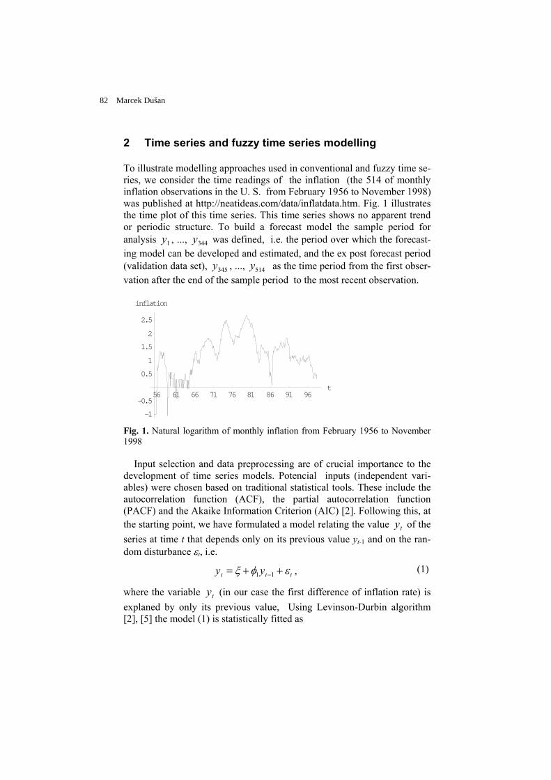
2 Time series and fuzzy time series modelling

To illustrate modelling approaches used in conventional and fuzzy time se-ries, we consider the time readings of the inflation (the 514 of monthlyinflation observations in the U. S. from February 1956 to November 1998)was published at http://neatideas.com/data/inflatdata.htm. Fig. 1 illustratesthe time plot of this time series. This time series shows no apparent trendor periodic structure. To build a forecast model the sample period foranalysis y1 , ..., y344 was defined, i.e. the period over which the forecast-ing model can be developed and estimated, and the ex post forecast period(validation data set), y345 , ..., y514 as the time period from the first obser-vation after the end of the sample period to the most recent observation.

56 61 66 71 76 81 86 91 96t

-1

-0.5

0.5

1

1.5

2

2.5

inflation

Fig. 1. Natural logarithm of monthly inflation from February 1956 to November1998

Input selection and data preprocessing are of crucial importance to thedevelopment of time series models. Potencial inputs (independent vari-ables) were chosen based on traditional statistical tools. These include theautocorrelation function (ACF), the partial autocorrelation function(PACF) and the Akaike Information Criterion (AIC) [2]. Following this, atthe starting point, we have formulated a model relating the value ty of theseries at time t that depends only on its previous value yt-1 and on the ran-dom disturbance εt, i.e.

y yt t t= + +−ξ φ ε1 1 , (1)

where the variable ty (in our case the first difference of inflation rate) isexplaned by only its previous value, Using Levinson-Durbin algorithm[2], [5] the model (1) is statistically fitted as

82 Marcek Dušan

$ ,y yt t= − −0 1248 1 (2)

In contrast to the conventional time series, the observations of fuzzytime series are fuzzy sets (the observations of conventional time series arereal numbers), the universes of discourse for the fuzzy sets are subsets of

1ℜ , where 1ℜ is the set of real numbers, either naturally or artificially de-fined. Song and Chisson [6] give a thorough treatment of these models.Let Xt , (t = ..., 1, 2, ...), a subset of 1ℜ , be the universe of discourse onwhich fuzzy sets yt

i , (i = 1, 2, ...) are defined and Yt is the collection ofyt

i , (i = 1, 2, ...). Then Yt , (t = ..., 1, 2, ...) is called a fuzzy time series onXt , (t = ..., 1, 2, ...).

The fuzzy time series modelling procedure consists of an implementa-tion of several steps, usually as follows:

1. Define the input-output variables and the universes of discourse.2. Define (collect) linguistic values and fuzzy sets on the universes of dis-

course.3. Define (find) fuzzy relations (fuzzy rules).4. Apply the input to the model and compute the output.5. Defuzzify the output of the model.

Firstly, in the fuzzification process, we specified input and output vari-ables. The input variable xt−1 is the lagged first difference of inflation val-ues yt and is calculated as 1−tx = 1−ty - 2−ty , t = 3, 4, ... . The outputvariable xt is the first difference of inflation values yt and is calculatedas tx = ty - 1−ty , t = 2, 3, ... .. The variable ranges are as follows:

- 0,75 ≤ xt , xt−1≤ 0,75 .

These ranges define the universe of discourse within which the data of1−tx and tx are, and on which the fuzzy sets have to be, specified. The

universes of discourse were partioned into the seven intervals.Next, we specified the fuzzy-set values of the input and output fuzzy

variables. The fuzzy sets numerically represented linguistic terms. Eachfuzzy variable assumed seven fuzzy-set values as follows: NL: NegativeLarge, NM: Negative Medium, NS: Negative Small, Z: Zero, PS: PositiveSmall, PM: Positive Medium, PL: Positive Large.

Fuzzy sets contain elements with degrees of membership. Fuzzy mem-bership functions can have different shapes. The triangular membership

Generating fuzzy rules for financial time series by ... 83

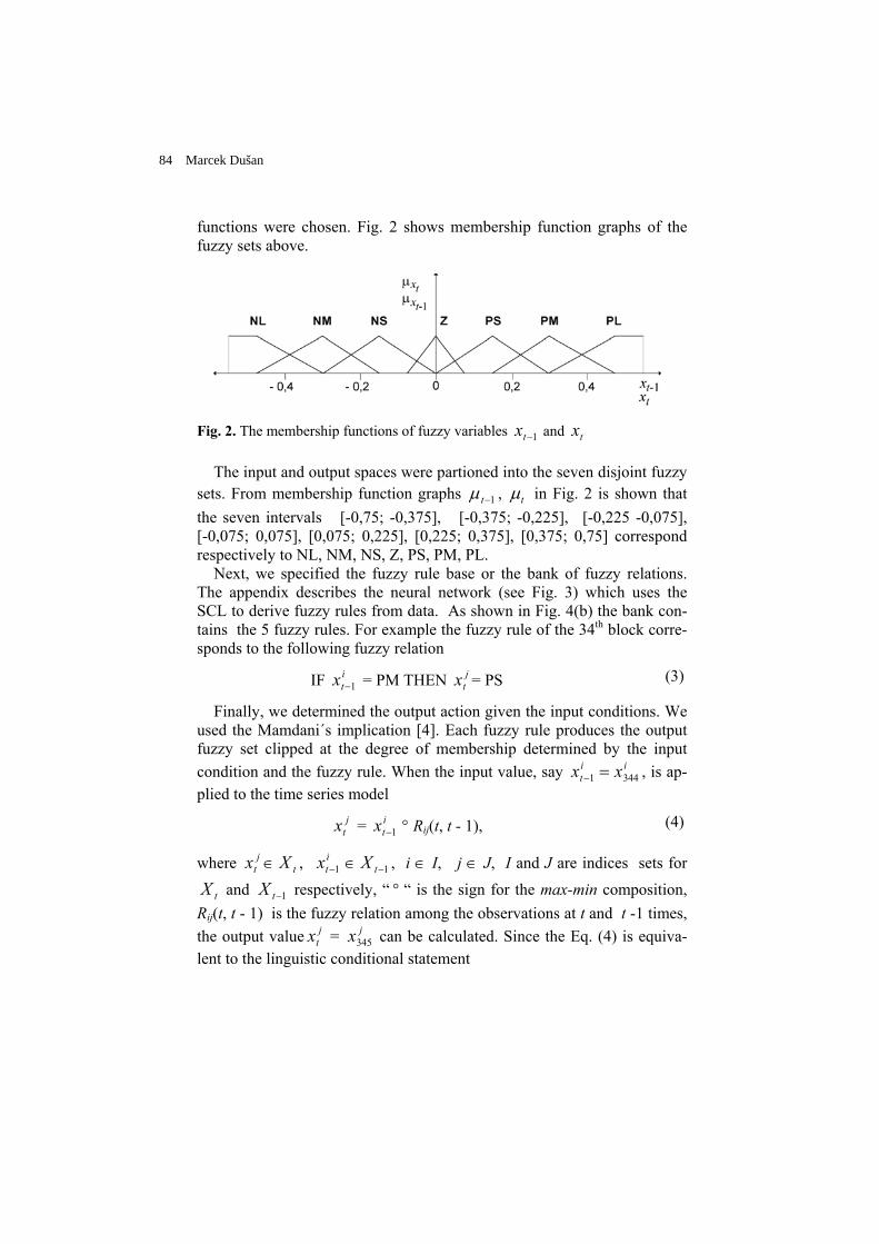
functions were chosen. Fig. 2 shows membership function graphs of thefuzzy sets above.

Fig. 2. The membership functions of fuzzy variables 1−tx and tx

The input and output spaces were partioned into the seven disjoint fuzzysets. From membership function graphs 1−tµ , µt in Fig. 2 is shown thatthe seven intervals [-0,75; -0,375], [-0,375; -0,225], [-0,225 -0,075],[-0,075; 0,075], [0,075; 0,225], [0,225; 0,375], [0,375; 0,75] correspondrespectively to NL, NM, NS, Z, PS, PM, PL.

Next, we specified the fuzzy rule base or the bank of fuzzy relations.The appendix describes the neural network (see Fig. 3) which uses theSCL to derive fuzzy rules from data. As shown in Fig. 4(b) the bank con-tains the 5 fuzzy rules. For example the fuzzy rule of the 34th block corre-sponds to the following fuzzy relation

IF xti−1 = PM THEN xt

j = PS (3)

Finally, we determined the output action given the input conditions. Weused the Mamdani´s implication [4]. Each fuzzy rule produces the outputfuzzy set clipped at the degree of membership determined by the inputcondition and the fuzzy rule. When the input value, say x xt

i i− =1 344 , is ap-

plied to the time series modelj

tx = itx 1− ° Rij(t, t - 1), (4)

where jtx ∈ tX , i

tx 1− ∈ 1−tX , i ∈ I, j ∈ J, I and J are indices sets for

tX and 1−tX respectively, “ ° “ is the sign for the max-min composition,Rij(t, t - 1) is the fuzzy relation among the observations at t and t -1 times,the output value xt

j = x j345 can be calculated. Since the Eq. (4) is equiva-

lent to the linguistic conditional statement

84 Marcek Dušan

”if itx 1− then j

tx ”, (5)

we have )1,( −ttRij = itx 1− × j

tx , where “×“ is the Cartesian product.

It is possible to compute the output fuzzy value xtj by the following

simple procedure consisting of three steps:

− Compute the membership function values µNL( xt−1), µNM( xt−1), ...,µPL( xt−1) for the input xt−1 using the membership functions pictured inFig. 2.

− Substitute the computed membership function values in fuzzy relations(4), (5).

− Apply the max-min composition to obtain the resulting value xtj of

fuzzy relations.

Following the above principles, we have obtained the predicted fuzzyvalue for the inflation xt = x j

345 = 0,74933.To obtain a simple numerical value in the output universe of discourse,

a conversion of the fuzzy output is needed. This step is called defuzzifica-tion. The simplest defuzzification scheme seeks for the value $xt that is ofmiddle membership in the output fuzzy set. Hence, this defuzzificationmethod is called the Middle of Maxima, abbreviated MOM. Following thismethod, we have obtained the predicted value for the $x345 = - 0,15 . Theremaining forecasts for ex post forecast period t = 346, 347, ... may begenerated similarly.

3 Generating fuzzy rules with product-space clustering

The neural network pictured in Fig. 3 was used to generate structuredknowledge of the form „if A, then B“ from a set of numerical input-outputdata. In Section 2 we defined cell edges with the seven intervals of thefuzzy-set values in Fig. 2. The interval - 0,75 ≤ xt , xt−1≤ 0,75 was parti-tioned into seven nonuniform subintervals that represented the sevenfuzzy-set values NL, NM, NS, Z, PS, PM, and PL assumed by fuzzy vari-ables xt−1 and xt . The Cartesian product of these subsets defines7 × 7 = 49 fuzzy cells in the input-output product space 2ℜ .

We can represent all possible fuzzy rules as 7-by-7 linguistic matrix (seeFig. 4). The idea is to categorise a given set or distribution of input vectors


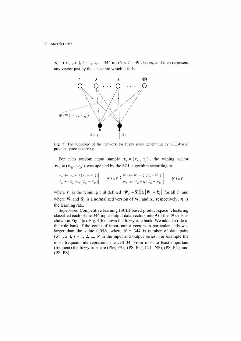
x t = ( xt−1, xt ), t = 1, 2, ..., 344 into 7 × 7 = 49 classes, and then representany vector just by the class into which it falls.

Fig. 3. The topology of the network for fuzzy rules generating by SCL-basedproduct-space clustering

For each random input sample x t t tx x= −( , )1 , the wining vector),( 21 iii ww ′′′ =w was updated by the SCL algorithm according to

~ ~ (~ ~ )~ ~ (~ ~ )

w w x ww w x w

if i ii i t i

i i t i

1 1 1 1

2 2 2 2

′

′

← + −

← + −

= ′

η

η ;

~ ~ (~ ~ )~ ~ (~ ~ )

w w x ww w x w

if i ii i t i

i i t i

1 1 1 1

2 2 2 2

′

′

← − −

← − −

≠ ′

η

η

where ′i is the winning unit defined ~ ~ ~ ~w x w x′ − ≤ −i t i t for all i , andwhere ~w i and ~xt is a normalized version of w i and x t respectively, η isthe learning rate.

Supervised Competitive learning (SCL)-based product-space clusteringclassified each of the 344 input-output data vectors into 9 of the 49 cells asshown in Fig. 4(a). Fig. 4(b) shows the fuzzy rule bank. We added a rule tothe rule bank if the count of input-output vectors in particular cells waslarger than the value 0,05N, where N = 344 is number of data pairs( xt−1, xt ), t = 1, 2, ..., N in the input and output series. For example themost frequent rule represents the cell 34. From most to least important(frequent) the fuzzy rules are (PM; PS), (PS; PL), (NL; NS), (PS; PL), and(PS; PS).

86 Marcek Dušan

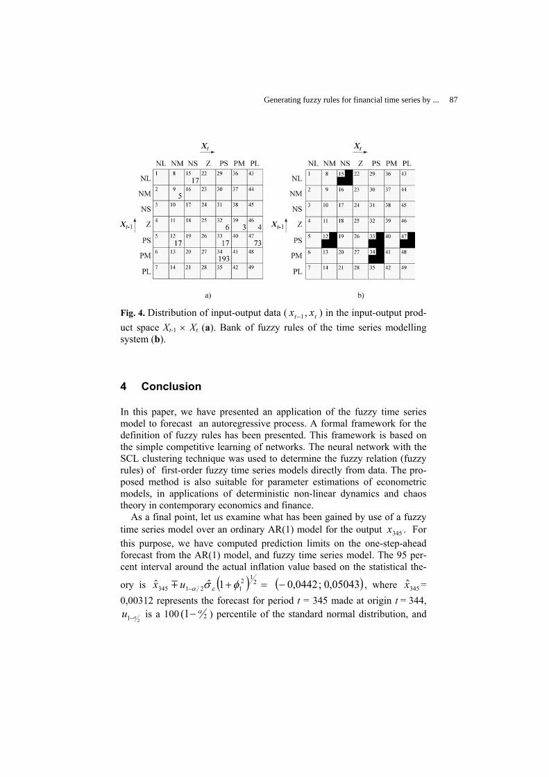
Fig. 4. Distribution of input-output data ( xt−1, xt ) in the input-output prod-uct space Xt-1 × Xt (a). Bank of fuzzy rules of the time series modellingsystem (b).

4 Conclusion

In this paper, we have presented an application of the fuzzy time seriesmodel to forecast an autoregressive process. A formal framework for thedefinition of fuzzy rules has been presented. This framework is based onthe simple competitive learning of networks. The neural network with theSCL clustering technique was used to determine the fuzzy relation (fuzzyrules) of first-order fuzzy time series models directly from data. The pro-posed method is also suitable for parameter estimations of econometricmodels, in applications of deterministic non-linear dynamics and chaostheory in contemporary economics and finance.

As a final point, let us examine what has been gained by use of a fuzzytime series model over an ordinary AR(1) model for the output x345 . Forthis purpose, we have computed prediction limits on the one-step-aheadforecast from the AR(1) model, and fuzzy time series model. The 95 per-cent interval around the actual inflation value based on the statistical the-

ory is ( ) =+−2

12121345 1ˆˆ φσ εαux m ( )05043,0;0442,0− , where $x345 =

0,00312 represents the forecast for period t = 345 made at origin t = 344,

21 α−u is a 100 (1 2− α ) percentile of the standard normal distribution, and


$σε an estimate of the standard deviation of the noise. An intuitive methodfor constructing confidence intervals for fuzzy time series model is simplythe defuzzification method First of Maxima and First of Minima to obtainprediction limits on the one-step-ahead forecast. In our example, the „con-fidence“ interval for fuzzy time series value $x345 = -0,15 is (-0,30256 to0,3088). The sign of the actual value for the AR(1) model is opposite tothe forecast value sign.

The method may be of real usefulness in practical applications whereusually the expert can not explain linguistically, what control actions theprocess takes or there is no knowledge of the process.

Because the results were based of chosen inflation rates and data set,they were difficult to generalize in others situations. Yet, the results cer-tainly provide a rational way for improvement of forecasting ability inchaotic economic systems.

Acknowledgement

This work is supported by Slovak grant foundation under the grantNo. 1/9183/02.

References

1. Box, G. E. P., and G. M. Jenkins: Time Series Analysis, Forecastingand Control, Holden-Day, San Francisco, CA, 1970

2. Brockwell, P.J. and Davis, R.A.: Time Series: Theory and Methods.Springer-Verlag, New York, 1987

3. Kosko, B.: Neural networks and fuzzy systems - a dynamical systemsapproach to machine intelligence. Prentice-Hall Int., Inc. 1992

4. Mamdani, E., H.: Application of a fuzzy logic to approximate rea-soning using linguistic synthesis. IEEE Trans. Comput. 26 (1977), pp.1182-1191

5. Morettin, P., A.: The Levinson algorithm and its applications in timeseries analysis. International Statistical Review, 52, 1984, pp. 83-92

6. Song, Q., Chisson, B., S.: Fuzzy time series and its models. FuzzySets and Systems, 54, 1993, pp. 269-277

7. Sugeno, M., and Yasukawa, T.: A fuzzy-logic-based approach toquantitative modelling. IEEE Trans. Fuzzy System. Vol. 1, No. 1,Feb. 1993, pp. 7-31

88 Marcek Dušan

Pattern Recognition through Perceptually Important Points in Financial Time Series

Gul Zaib, Uzair Ahmed & Arshad Ali

National University of Sciences and Technology (NUST), NUST In-stitute of Information Technology, Chaklala Scheme III, Rawal-pindi, Pakistan Phone: +92-51-9280658, Fax: +92-51-9280782 Email: gul.zaib,uzair.ahmed,[email protected]

Abstract Technical Analysis is a financial risk management practice that has been in use since the advent of stock market and Pattern Recognition is an indivisible part of it. There has been a lot of research in to pat-tern recognition in time series. Existing pattern recognition tech-niques lacks dynamic extensibility. They do not provide any inter-faces in order to include new patterns for recognition dynamically. This limits the operability of these techniques to a particular domain. This research devises a new technique for domain independent pat-tern recognition while giving sufficient speed and accuracy. This en-ables it to be used by critical Decision Support Systems for time se-ries of different domains. The system emulates human visual cognition process by implementing the concept of Perceptually Im-portant Points Identification (PIPI). Perceptually Important Points (PIP) represents minimal set of data points which are necessary to form a pattern. For dynamic inclusion of patterns a Pattern definition Language (PDL) has been conceptualized for defining patterns in time series by using declarative programming paradigm. This also results in domain independent pattern recognition without needing any modification. Keywords: stock pattern mining, pattern recognition, financial time series, soft computing, declarative programming, time series analy-sis, perceptual modelling, computer vision, non-linear pattern rec-ognition, modelling human cognition

Introduction

Historic time series data is one of the most precious assets of mod-ern business and scientific research entities. Modern decision sup-port systems (DSS) are expected to execute important policies based upon patterns occurring in time series This Makes pattern recogni-tion and integral part of any future DSS. Pattern recognition is primarily a human cognitive faculty. Depend-ing upon an individual’s ability faces severe limitations. Its expertise vary among individuals, thus it can not provide basis for the deci-sions involving a high degree of risk. Secondly scanning huge amounts of data to for a single pattern or even recursively scanning it for multiple patterns is an humanely impossible task [1]. Still hu-man cognitive process is indispensable as all the small non lineari-ties and variation in patterns can not be captured through traditional parametric approaches. So we develop a system which utilizes the strengths of human cognitive process while removing its above dis-cussed weaknesses. We develop a system that closely imitates human faculty of pat-tern recognition and is called Perceptually Important Point Identifi-cation (PIPI). Briefly, it first divides the time series being scanned in to seg-ments. Once segmentation is completed the whole system explores the time series to discover PIPs. Once pips in a specific formation are found, system classifies that segment of time series in which PIPs are found as making the desired pattern. To extend the system the user simply has to define the pattern in our specified PDL (Pat-tern Definition Language). The system would then be ready to start looking for that new pattern in large volumes of Time Series. Rest of the paper is structured as follows. First the status of cur-rent research in the field of pattern recognition is explained. A PIP (Perceptually Important Point) will be defined; also the advantages gained by using perceptually important points instead of traditional parametric techniques are given after that. Then whole PIPI is ex-plained along with an example of stock time series. The structure of PDL and the architecture of its parser and interpreter will be given after that. The result of two performance gauging experiments done on PIPI are given and in the end there is conclusion.

90 Zaib Gul, Ahmed Uzair and Ali Arshad

Previous work

[8] Have used hierarchal pattern analysis for pattern recognition in time series. Hierarchical pattern analysis The problems with this technique are a) a pattern must be seen at least once to be recog-nized, b) The user can not him self add patterns to it. [7] Applied self organizing maps to the process of pattern discov-ery for making neural network training for pattern discovery effi-cient and accurate. [5] Has presented his technique of SNN (Single nearest neighbor) for pattern detection in long memory systems. This approach is extremely slow and further becomes slower as the time series or size of the segment becomes larger. [6] pattern matching utilizes distance measure by storing the Euclidian distance between fixed points, and then compares that dis-tance with the previous time series to locate a pattern. Most of the research has been mainly focused on two attributes of pattern recognition i.e. efficiency and accuracy. There is still a need for a pattern recognition technique which should be able to work across domains, should be extensible enough, meaning that once it has been trained to recognize certain patterns at development time, it can be extended later to add more patterns. The features of extensi-bility and domain independence should not be achieved at the cost of efficiency or accuracy i.e. it should be efficient enough to be used in interactive system, should be accurate enough so that people could rely on it for critical decisions.

P.I.P.I Perceptually Important Point Identification:

P.I.P (Perceptually Important Points) definition

Time series are made up of finite but very large number of data points if we consider a pattern on a time series it will be subset of the points of making the whole time series, but even all those points are not required for pattern recognition. If we concentrate on even a smaller set of point we are still able to recognize pattern. These points which are necessary for pattern recognition are termed in this paper as Perceptually Important points or PIPS.

Pattern Recognition through Perceptually Important Points in Financial Time Series 91

Challenges requiring the use of PIPS

• Domain Independent: The pattern recognition should work across domains the technique which should be able to ignore differences in the properties of time series. It should be flexible to work across domains

• Time Unit Independent: Time series can be on varying time scales within and across domains so there should be such a technique which is able to work no matter the time scale is hours, years or any thing in between as long as it is constant within a pattern.

• Highly Non Linear Patterns: Most of the patterns can not be de-fined strictly in terms of shape. Small non linearities will always exist in time and value.

• Missing Data: Most of the time several data values between 2 ranges of time series are missing. Thus we must also implement some method to overcome the problem of missing data

• Need for a smoothing function: Time series having a lot of small non lineraites confuse the traditional techniques, so the data is passed thorough filters in order to smooth it.

Advantages of using PIPI

1. Time Unit Independence: When using PIPS we get independent from time unit, it does not matter what unit of time each data point of time series enclose as long as all the PIPs in the pattern belong to same time unit.

2. No need of a smoothing function: When using PIPs there is no need of a smoothing function as highly noisy data does not affect accuracy. This is because we do not need to feed whole time se-ries to the technique. Only we need the data related to PIPs.

3. Missing data do not effect accuracy: We do not need any filter to fill in missing data as long as the data points that will form the PIPs of the pattern exist, on these PIPs will be sufficient to do the pattern recognition

4. Pattern Definition Feasible: Further more when using PIPs, pat-tern definition is feasible as we only need some way to represent the PIPs in the time series. It also represents their relative position


in the pattern in order to make our algorithm domain independent and evolvable.

PIP identification algorithm

1. Find Minimum and Maximum value of time series for this time series. For this time series min and max values are 2.5 and 20.5 respectively.

2. Divide whole time series in to segments with a segmentation fac-tor. The segmentation factor is fixed for time series belonging to each domain for example it is 1.5 % for stock data. However it can too be varied to increase the accuracy of recognition algo-rithm for each domain. The density of points lower as we go up, so the band size must increase in order to allow for lowering den-sity. For the sample time series the number of bands will be 24

3. Start PIP Identification Process once the time series has been segmented. For this we first; arrange the segments in order by their volume, because almost all the pattern starts from the seg-ment having high density of data points. In this sample series this segment is the segment 1.

4. Find Neighboring Pips that lie in the bottom layer, these are marked with red arrows, check if they satisfy the pattern i.e. in same band number is greater than four then we move on to upper layer so that the shoulder should be completed, now we will find the points in the upper layer at the mean of point already found, but not at exact mean, give or take a single time unit

5. Remember the matching points found, if they become equal to a specified number then the pattern is successfully detected e.g. for Head and Shoulder Pattern there must exist at least eight points.

Pattern Definition Language

PDL requirements

PDL (Pattern Definition Language) makes the system extensible, so it should be capable of modeling different aspects of the pattern. Each PIPs has two properties, the value on x axis which is always


some unit of time and the value on y axis which is different for each time series. To define the relation ship between PIPs we will also take, the distance of one PIP from another PIP in time and the dis-tance of one PIP from another PIP in value One of the strengths of human cognition is its ability to approxi-mate patterns. Approximation means that humans have the capabil-ity to ignore small difference and take a look at the bigger picture to recognize a pattern. So the PDL designed should be capable of:

1. Defining the actual change in value that must be present be-tween one PIP and the next.

2. The variation that can take place in the value change, i.e. the number of value units around the original where a PIP can exist if it’s not found at the original change position.

3. As it is quite possible that the next PIP is not exactly at the specified time interval so we must also specify a variation for time and for value.

4. The variation or interval may be defined with respect to any previous point found. For example if the last point we found is “n”. A requirement comes to find point that is 3 time units a head of point n-3 i.e. a point found three points back. So the PDL should be capable of doing this

5. Moreover the variation can be till the end of time series so there must be some way to specify the end of time series along X axis or Y axis.

PDL structure

Table 1, shows different key symbols. Symbol Usage N Specify variation to the end of

time series +,- Define the direction of finding

next PIP: +: Move forward in time or


move higher in value -: Move previous in time or lower in value

|value| Any value written between | | in-dicate the reference to any pre-vious point i.e. |2| means move to point found 2 points back.

/ The line separator used in PDL, just like the use of “;”.

+ Used to show the start of a pat-tern i.e. to indicate that system should pick up the first point to start looking for new pattern

Conclusion

PIPI is a simple yet powerful technique to recognize patterns. It im-proves over previous work in this area in the following aspects

• It provides a high level abstraction of time series patterns, rather then treating pattern discovery process as a black box – something that the user may be uncomfortable with

• Its specification is close to how human keep patterns in memory, where as its working closely imitates the human way of pattern recognition

• PDL let us define patterns based upon the relationships be-tween perceptually important points. It makes the system ex-tensible in two aspects. Enabling dynamic inclusion of pat-tern and also the technique lends it self to be used across the domains without any modification.

A PIPI prototype implementation exhibits very impressive re-source utilization during the detection process of the pattern and also shows highly optimized time series search. The experimental data was of year 1995 for share prices of CNN. Besides we also used a hypothetical data of 87 years for stress tests. A graphical user inter-

3 2 4 0 1 5 6


face is the future direction of this. This shall enable visual usage of PDL. It will help the user to define a pattern by marking the segment of time series in which the pattern occurs.

REFRENCES

[1] Hedge, Human Information Processing – Pattern Recognition, Decisions And Attention,. Cornell University 1999.

[2] Frietman, XCG-NEUROPC: Senter R & D program, Faculty of Applied Phys-ics, Delft University of Technology, Delft, Netherlands 1994.

[3] Identifying Seismicity Patterns Leading Flank Eruptions At Mt. Etna Volcano During 1981-1996, Center for Theoretical Physics, Laboratory for Nuclear Sciences and Department of Physics, Massachusetts Institute of Technology, Cambridge, Massachusetts 1999

[4] Tarr, Visual Pattern Recognition, Brown University 1996 [5] Singh,A Long Memory Pattern Modelling And Recognition System For Fi-

nancial Time-Series Forecasting, University of Exeter Department of Com-puter Science Prince of Wales Road Exeter 2001

[6]Pratt LOCATING PATTERNS IN DISCRETE TIME-SERIES Department of Computer Science and Engineering College of Engineering University of South Florida 2001

[7]Fu, Pattern Discovery From Stock Time Series Using Self-Organizing Maps, KDD2001 Workshop on Temporal Data Mining,

[8] Ge, Pattern Matching in Financial Time Series Data, third conference on Knowledge Discovery in Databases and Data Mining 2000


Soft Clustering for Funds Management Style Analysis: Out-of-sample Predictability

Paul Lajbcygier and Asjad Yahya

School of Business Systems,

Monash University, Clayton, Australia.

Email:[email protected]

Abstract Mutual funds are generally grouped on the basis of their investment objectives. Inves-

tors use these groupings, or ‘styles’, to make investment decisions and compare the per-formance of fund managers against appropriate indexes. Various authors have criticized the traditional classification approaches because they are made on the basis of funds’ stated ob-jectives, not the actual fund styles and are therefore often misclassified. [6] introduced the General Style Classification (GSC) approach as an alternative to the traditional technique which uses statistical (rather than stated) objectives. Results of their study suggest that in-vestment style boundaries are continuous rather than “hard”. In this work, we classify mu-tual funds using a soft clustering technique (Fuzzy-C-Means) and compare it with a hard clustering technique (GSC). This comparison demonstrates soft clustering can predict mu-tual fund performance better out-of-sample.

INTRODUCTION

The mutual funds industry has grown considerably over the years. Be-tween 1995 and 2000, the number of mutual funds worldwide nearly dou-bled from 34,992 to 53,450 and assets managed by these funds nearly tri-pled from US $5.386 trillion to US $12.152 trillion [1]. In the United States alone, 47.0 million households had a stake in mutual funds in 2002 [2].

The fact that independent sources like Morningstar publish their own styles, despite officially stated objectives by the funds, highlights a prob-lem faced by the mutual fund industry: misclassification of funds.

To address the problem of fund misclassification, [6] developed an al-ternative to the traditional techniques. The Generalized Style Classification (GSC) approach uses past returns to group funds into a pre-determined number of styles. The underlying concept is that funds following similar

investment patterns, irrespective of their objectives, will have similar re-turns and hence will be placed in one group when statistically clustered on the basis of past performance. The use of past returns has the added advan-tage that GSC is not fooled by window-dressing1. Empirical evidence sug-gests that this technique is superior to traditional industry classifications in predicting cross-sectional future and past performances [6-7].

Results of the study in [6] showed that the investment actions of the mu-tual fund managers in America could be explained by eight different in-vestment styles. Each style was formed using the GSC technology, and is comprised of a combination of a number of traditional style definitions. For example, the ‘Glamour’ style defined in [6] consists primarily of Morningstar ‘growth’ and ‘small company’ funds. This example illustrates that in-practice fund managers do not restrict themselves solely to one in-vestment style and suggests that the style categories have continuous rather than “hard” boundaries. If this holds true, the analysis of mutual funds through soft clustering should yield greater insight into the actions of fund managers as opposed to an analysis through the use of a hard clustering approach (i.e. the GSC). The main problem with the latter is that, despite the fact that the results suggest the existence of continuous style bounda-ries, the algorithm places each fund exclusively into only one cluster. Soft clustering, on the other hand, ‘divides’ the fund among a number of clus-ters by assigning membership values to each of the pre-defined styles. This permits fund managers to belong to multiple investment styles.

The main aim of this paper to is to establish a rationale for switching to the use of soft clustering from hard clustering for mutual funds analysis. This is achieved by illustrating the advantages of analyzing a dataset of American mutual fund returns using a soft clustering approach (Fuzzy-C-Means) as compared to an analysis using a hard clustering approach (GSC) and, in particular, comparing their out-of-sample mutual fund return pre-dictions.

METHODOLOGY AND DATA

We have shown ([14]) that the theoretical returns generating process is consistent with the use of k-means clustering. This motivates the use of the quasi k-means clustering approaches used in this study –– the ‘hard’ clustering GSC, and its soft clustering analog –– Fuzzy-C-Means. The de- 1 At the end of each period, fund managers often sell off poor performers in the

portfolio and/or change the apparent strategy of the fund. This practice is known as ‘Window dressing’.

98 Lajbcygier Paul and Yahya Asjad

tails of their derivation (and tweaking) are omitted here due to space con-straints, however they are discussed in [14].

Fuzzy-C-Means, which is a generalization of the “hard” k-means [8] clustering approach, was chosen because: it and the GSC are similar to k-means clustering and therefore can be justified based on the theoretical re-turn generating process. In particular, mutual fund return predictions are compared using the GSC and Fuzzy-C-Means technology. We find that the Fuzzy-C-Means approach yields more accurate out-of-sample predictions.

The dataset was made up of 42 monthly returns, from 31 January 1997 to 30 June 2000, for 7594 U.S. equity funds. As is common with most mu-tual funds datasets, a number of values were missing2.

RESULTS

This section discusses the results comparing GSC and Fuzzy-C-Means. It does this by determining which approach –– GSC or Fuzzy-C-Means –– provides more accurate out-of-sample predictions of funds management performance.

When attempting to compare different approaches for the estima-tion of funds management style we want to know how one approach can be said to be better than another. A key issue is that “there are no generally accepted standards for comparing style classifications” [6]. So, [6] borrowed “a natural measure from the asset pricing model” and used regression to measure the performance of GSC against other classification techniques, including the traditional methodology. Fund returns were cross-sectionally regressed on a matrix of dummy variables, which indicated whether a fund be-longed to a particular style. This exercise was carried out for both GSC and industry-based classifications. A comparison of adjusted R2s helped identify the classification technique with superior predic-

2 Missing returns were represented by ‘-95’ in the dataset. The GSC algorithm was designed to handle missing values, but results for Fuzzy-C-Means would have been distorted if unfiltered data had been used. Three methods were considered to overcome this problem: eliminating time series and/or funds with missing values beyond an acceptable threshold level; replacing missing returns with average re-turns; replacing missing values with zeros. After careful consideration of the ef-fects these techniques would have on the final results, missing values were han-dled the way the GSC ([6]) algorithm handles them also by replacing missing returns with zeros. This ensured consistency between the two techniques.

Soft clustering for funds management style analysis: Out-of-sample Predictability 99

tive ability. “This procedure resembles classical time-series, cross-section tests of pricing models, except that the cross-sectional re-gressors are not loadings but a matrix of dummy variables” [6].

The methodology used in this study to compare Fuzzy-C-Means with GSC is a variation of the technique described above. The fol-lowing section presents the results of the regression analysis, along with details of deviations from the technique originally used by [6].

[6] used a twenty-four month rolling period of fund returns, instead of the entire dataset, for the cross-sectional regression. The use of a rolling window, which was moved forward twelve months at a time, relaxed the assumption that funds belonged to the same style over the entire period [6]. This exercise was carried out for both GSC and industry classifications. Adjusted R2s were compared to identify the classification technique that did a better job of explaining cross-sectional variance.

The regression analysis carried out in this study differs from the [6] methodology in two key ways. Firstly, instead of a twenty-four month roll-ing window, a thirty-six month period was used for the regression3. Sec-ondly, due to the shortage of available data, the returns window was rolled on a month-by-month basis instead of a yearly basis. [6] found that the in-dustry-based styles significantly under-performed other techniques when they used rolling month-by-month returns. This was due to the fact that the other techniques used data subsequent to the publication date of the indus-try styles to classify funds. Thus, in order to overcome this problem, [6] used a one-year test period. However, this study is not constrained by this limitation: both GSC and Fuzzy-C-Means use the same data to classify funds.

Table 1 reports the results of out-of-sample cross-sectional regressions for GSC and Fuzzy-C-Means. Since both GSC and Fuzzy-C-Means clas-sify funds into the same number of styles, simple R2s were used instead of adjusted R2s to compare their predictive ability. The results appear to indi-cate that Fuzzy-C-Means does a better job of classifying funds than the GSC. Apart from the first two test periods, the R2s for the Fuzzy styles are significantly higher than those for GSC. Thus, the results seem to imply that the use of soft clustering in general, and Fuzzy-C-Means in particular, can provide more accurate prediction than hard-clustering.

3 [6] found that the use of rolling month-by-month returns for 24, 36, 48 and 60

months to classify funds yielded qualitatively similar results. Thus, due to the length of time it takes GSC to classify funds for each set of returns, a thirty-six month period was used.


Table 1 Regression Results

R-squares GSC Fuzzy-C-MeansJan 2000 0.112 0.1 Feb 2000 0.5504 0.5576 Mar 2000 0.4647 0.5415 Apr 2000 0.4232 0.5238 May 2000 0.4529 0.5557 Jun 2000 0.4983 0.5952 Mean 0.4169 0.479 Median 0.4588 0.5486 Std. Dev 0.1556 0.1871

A key consideration regarding this analysis is that, while the results

seem to support the theoretical justification presented earlier in the study to switch from the a hard to a soft clustering approach, a number of caveats must kept in mind while interpreting them. Firstly, the test was conducted over a very short period: as mentioned earlier, due to the amount of time it takes GSC to classify each set of funds, a larger returns window was cho-sen to decrease the computation time, which led to fewer test periods. The GSC styles perform slightly better than their Fuzzy counterparts in the first test period. It is possible that GSC does a superior job of classifying funds prior to this period. Secondly, due to lack of availability of data, the re-turns window was rolled on a monthly basis. The use of such a small roll-ing period, combined with the small number of test periods, could have re-sulted in spurious results. Lastly, the presence of missing values in the test periods decreases the reliability of the results. Thus, although these results warrant further analysis into the use of soft clustering for style analysis, they should not be used as the sole basis for the replacement of GSC with Fuzzy-C-Means.

CONCLUSION

In this work we have introduced Fuzzy clustering to funds management style analysis and have found it to be a very powerful diagnostic tool. The technology appears to permit us to predict funds management performance out-of-sample more accurately than with the GSC technology.

Soft clustering for funds management style analysis: Out-of-sample Predictability 101

References

1. Investment Company Institute (2001) Mutual Fund Fact book 2. Investment Company Institute (2002) Equity Ownership in America 3. Kim, M., Shukla, R. and Tomas, M.: Journal of Economics and Business 52(4) (2000) 309-323 4. Wolper, Gregg (2002): Our style box should help you, not bind you

http://news.morningstar.com/doc/article/0,1,13564,00.html 5. Costello M.: The new growth (or old value) http://money.cnn.com/ 6. Brown, S. J. and Goetzmann, W. N.: Mutual Fund Styles. Journal of Financial Economics 43 (1997)

373-399 7. Lajbcygier, P. and Ong, M. Y.: Estimating the Number of Mutual Fund Styles Using the General-

ized Style Classification Approach and the Gap Statistic. Proceedings of Computational Intelli-gence in Finance (2003) IEEE Press

8. Hartigan, J. A.: Clustering Algorithms, Wiley, New York (1975) 9. Bezdek, J. C.: Pattern Recognition with Fuzzy Objective Function Algorithms, Plenum Press, New

York (1981) 10. Klir, G. J. and Yuan B.: Fuzzy Sets and Fuzzy Logic: Theory and Applications, Prentice Hall PTR,

New Jersey (1995) 11. Quandt, R.: Tests of the Hypothesis That a Linear Regression System Obeys Two Regimes. Journal

of American Statistical Association 55 (1960) 324-330 12. Odeh, I. O. A., McBratney A. B. and Chittleborough D. J.: Soil Pattern Recognition with Fuzzy-c-

means: Applications to Classification and Soil-Landform Interrelationships. Soil Science Society of America Journal 56 (1992) 505-516

13. Barès P. A., Gibson R. and Gyger S.: Style Consistency and Survival Probability in the Hedge Funds’ Industry. Swiss Federal Institute of Technology (2001)

14.Yaha A., Lajbcygier P., A rationale for using soft clustering for funds management style analysis", pp.412-416, Proceedings of the International Fuzzy Systems Association World Congress, Okyay Kaynak (Ed.), Istanbul, Turkey, June 26-29 2003, Figur Grafik & Matbaaclik Sanayi Ticaret Ltd.


Tuning the Fuzzy Classification Models with Various Learning Criteria: the Case of Credit Data Classification

Serhiy SHTOVBA, Olga PANKEVICH, and Georgios DOUNIAS

Department of Computer Based Information & Management Systems, Vinnitsa National Technical University, Vinnitsa, Ukraine [email protected] Department of Financial and Management Engineering, University of the Aegean, Chios, Greece, [email protected]

Abstract. In this paper we study the efficiency of various learning criteria for the proper tuning of a fuzzy classifier. Different cases of crisp and noisy class borders are considered, and a specific credit-risk application is discussed.

1 Introduction

Fuzzy rule–based systems are powerful tools which perform adequately in classification tasks related to various financial and economic decision-making problems, such as customer segmentation, credit-risk prediction, project evaluation, fraud detection, etc. [3, 4]. Fuzzy classifiers usually provide a good balance between decision accuracy and model transpar-ency. In this paper we study the efficiency of various learning criteria for the tuning process of a fuzzy classifier. Tuning corresponds to the search-process of weights of fuzzy if-then rules and parameters of the member-ship functions that minimize the difference between actual and inferred decisions. Cases of crisp and noisy class-separating curves with credit-risk assessing application are considered.

2 The Fuzzy Rule – Based Classifier

Let us consider a classifying system with n-inputs )x,,x,x( n21 K and one output y. The classification can be considered as the mapping:

( ) d,...,d,dyx,,x,xX m21n21 ∈→= K ,

where m21 d,...,d,d are decisions. The classification is performed with the aid of the following fuzzy knowledge base [1]:

U Ijk

1pjdywweightwith

n

1iaix jpjp,i

==→⎟

⎟

⎠

⎞

⎜⎜

⎝

⎛

== , m,1j = ,

(2.1)

where I is logical operation AND, U is logical operation OR, jp,ia de-

notes a fuzzy term for the evaluation of input ix in rule with number jp, ]1,0[w jp ∈ is a subjective degree of the expert’s confidence in rule with

number jp, jk is the number of rules corresponding to decision jd .

The membership degrees of an object ( )n21 x,,x,xX K= to decisions

jd ( m,1j = ) are calculated as follows [1]:

( ) ( )[ ] m,1j , x wX ijpn,1i

jpk,1p

dj

j =µ ⋅=µ==∧∨ , (2.2)

where )x( ijpµ denotes the membership function of the fuzzy term jp,ia ,

and )(∧∨ is the max (min) operation. The decision with the maximal fulfillment degree corresponds to object X:

( )(X)(X),...,(X),max arg y m21m21

dddd,...,d,d

µµµ= . (2.3)

3 Learning Criteria for Tuning the Fuzzy Classifier

Let us denote a fuzzy classifier by

)W,P,X(Fy = (3.1)

where X is an input vector, P is a vector of the membership functions’ pa-rameters in the knowledge base (2.1), W is a vector of the rule-weights in (2.1), and F is an input-output operator corresponding to (2.2) - (2.3).

We denote the training set by

( )rr y,X , M,1r = , (3.2)

104 Shtovba Serhiy, Pankevich Olga, and Dounias Georgios

where ( )n,r2,r1,rr x,...,x,xX = and ry are the input vector and its corre-sponding output for the input-output pair with number r.

The tuning corresponds to searching a vector (P, W) that minimizes the difference between actual (3.2) and inferred (3.1) decisions. This differ-ence may be defined in various ways.

Criterion 1. The percentage of misclassification is widely used as a learning criterion for diverse pattern recognition tasks. For this case, the tuning is equivalent to the following minimization:

minM1

M,1rr∑

=→∆ , where

⎩⎨⎧

=≠

=∆)W,P,X(Fy,0)W,P,X(Fy,1

rr

rrr . (3.3)

An advantage of this criterion is its simplicity and the clear interpreta-tion of values. The main drawback is the optimization difficulty related with plateau-shaped objective functions. It is often very hard to guess the suitable parameters of gradient optimizing routines, for example, the change in variables for finite difference gradient calculation.

Criterion 2. Let us apply fuzzification of the output variable in the train-ing set (3.2) as follows [1]:

⎪⎪⎭

⎪⎪⎬

⎫

==

====

mm21

2m21

1m21

dyif),d/1,...,d/0,d/0(y~...

dyif),d/0,...,d/1,d/0(y~dyif),d/0,...,d/0,d/1(y~

. (3.4)

The desirable values of the inferred membership grades (2.2) are equal to (3.4). Hence, the tuning problem may be now formulated as in the fol-lowing minimization [1]:

minW)P,,(X-)(yM1 M

1r

2m

1j

rrd jdj →⎥⎦

⎤⎢⎣⎡ µµ⋅ ∑ ∑

= =, (3.5)

where )(yrd jµ denotes the desirable membership degree according to

(3.4), and W)P,,(Xrjdµ denotes the inferred membership degree of ob-

ject rX by formula (2.2). The objective function in (3.5) does not have large plateaus, allowing

the use of gradient-based optimization methods. However, the optimal vec-tor for (3.5), sometimes does not obtain a minimal misclassification level

Tuning the fuzzy classification models ... 105

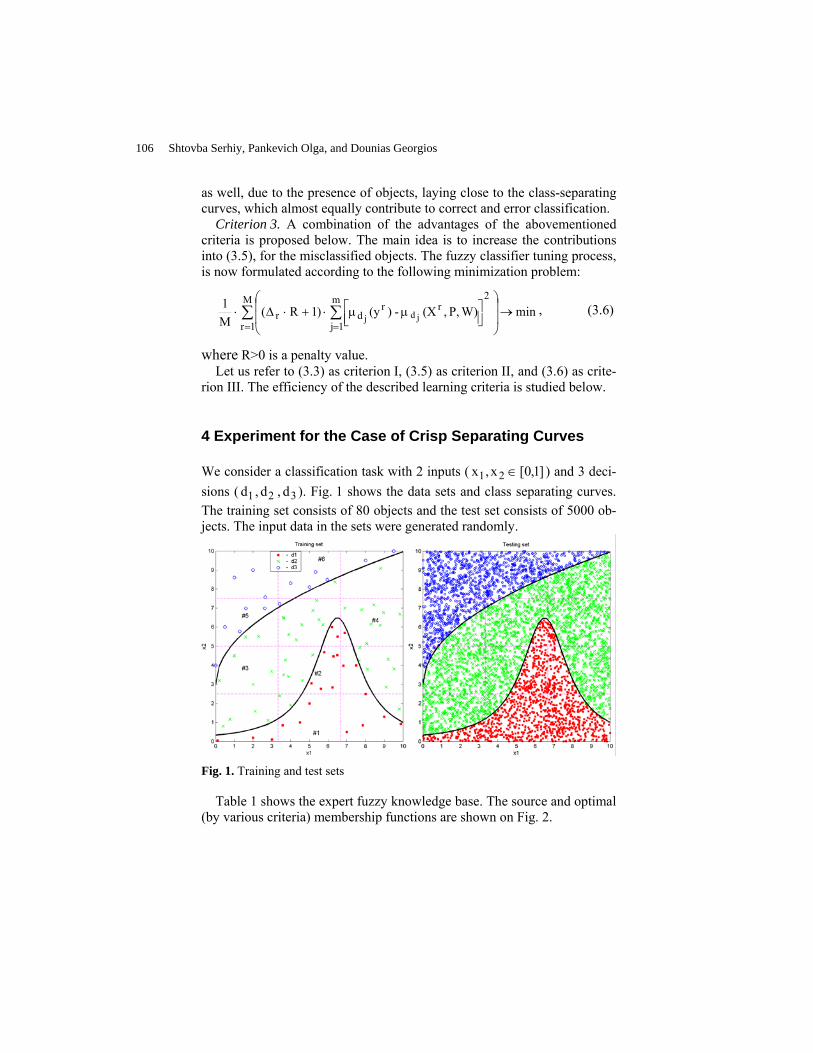
as well, due to the presence of objects, laying close to the class-separating curves, which almost equally contribute to correct and error classification.

Criterion 3. A combination of the advantages of the abovementioned criteria is proposed below. The main idea is to increase the contributions into (3.5), for the misclassified objects. The fuzzy classifier tuning process, is now formulated according to the following minimization problem:

minW)P,,(X-)(y)1R(M1 M

1r

2m

1j

rrdr jdj →⎟

⎟

⎠

⎞

⎜⎜

⎝

⎛

⎥⎦⎤

⎢⎣⎡ µµ⋅+⋅∆⋅ ∑ ∑

= =, (3.6)

where R>0 is a penalty value. Let us refer to (3.3) as criterion I, (3.5) as criterion II, and (3.6) as crite-

rion III. The efficiency of the described learning criteria is studied below.

4 Experiment for the Case of Crisp Separating Curves

We consider a classification task with 2 inputs ( ]1,0[x,x 21 ∈ ) and 3 deci-sions ( 1d , 2d , 3d ). Fig. 1 shows the data sets and class separating curves. The training set consists of 80 objects and the test set consists of 5000 ob-jects. The input data in the sets were generated randomly.

Fig. 1. Training and test sets

Table 1 shows the expert fuzzy knowledge base. The source and optimal (by various criteria) membership functions are shown on Fig. 2.


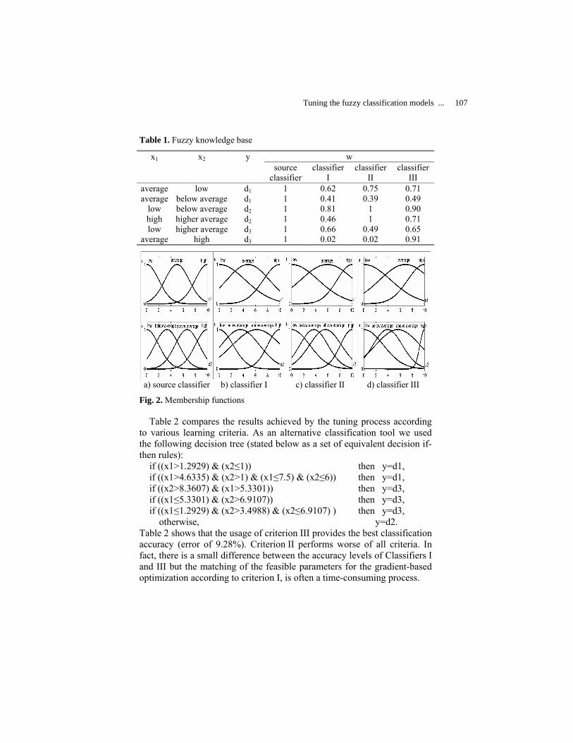
Table 1. Fuzzy knowledge base

w x1 x2 y source

classifier classifier

I classifier

II classifier

III average low d1 1 0.62 0.75 0.71 average below average d1 1 0.41 0.39 0.49

low below average d2 1 0.81 1 0.90 high higher average d2 1 0.46 1 0.71 low higher average d3 1 0.66 0.49 0.65

average high d3 1 0.02 0.02 0.91

a) source classifier b) classifier I c) classifier II d) classifier III

Fig. 2. Membership functions

Table 2 compares the results achieved by the tuning process according to various learning criteria. As an alternative classification tool we used the following decision tree (stated below as a set of equivalent decision if-then rules):

if ((x1>1.2929) & (x2≤1)) then y=d1, if ((x1>4.6335) & (x2>1) & (x1≤7.5) & (x2≤6)) then y=d1, if ((x2>8.3607) & (x1>5.3301)) then y=d3, if ((x1≤5.3301) & (x2>6.9107)) then y=d3, if ((x1≤1.2929) & (x2>3.4988) & (x2≤6.9107) ) then y=d3, otherwise, y=d2.

Table 2 shows that the usage of criterion III provides the best classification accuracy (error of 9.28%). Criterion II performs worse of all criteria. In fact, there is a small difference between the accuracy levels of Classifiers I and III but the matching of the feasible parameters for the gradient-based optimization according to criterion I, is often a time-consuming process.


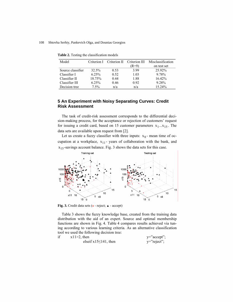
Table 2. Testing the classification models

Model Criterion I Criterion II Criterion III (R=9)

Misclassification on test set

Source classifier 32.5% 0.53 3.99 25.92% Classifier I 6.25% 0.52 1.03 9.78% Classifier II 18.75% 0.44 1.88 16.42% Classifier III 6.25% 0.46 0.92 9.28% Decision tree 7.5% n/a n/a 15.24%

5 An Experiment with Noisy Separating Curves: Credit Risk Assessment

The task of credit-risk assessment corresponds to the differential deci-sion-making process, for the acceptance or rejection of customers’ request for issuing a credit card, based on 15 customer parameters 151 x...x . The data sets are available upon request from [2].

Let us create a fuzzy classifier with three inputs: 8x - mean time of oc-cupation at a workplace, 11x - years of collaboration with the bank, and

15x -savings account balance. Fig. 3 shows the data sets for this case.

Fig. 3. Credit data sets ( - reject; - accept)

Table 3 shows the fuzzy knowledge base, created from the training data distribution with the aid of an expert. Source and optimal membership functions are shown in Fig. 4. Table 4 compares results achieved via tun-ing according to various learning criteria. As an alternative classification tool we used the following decision tree: if x11>2, then y=”accept”; elseif x15≤141, then y=”reject”;


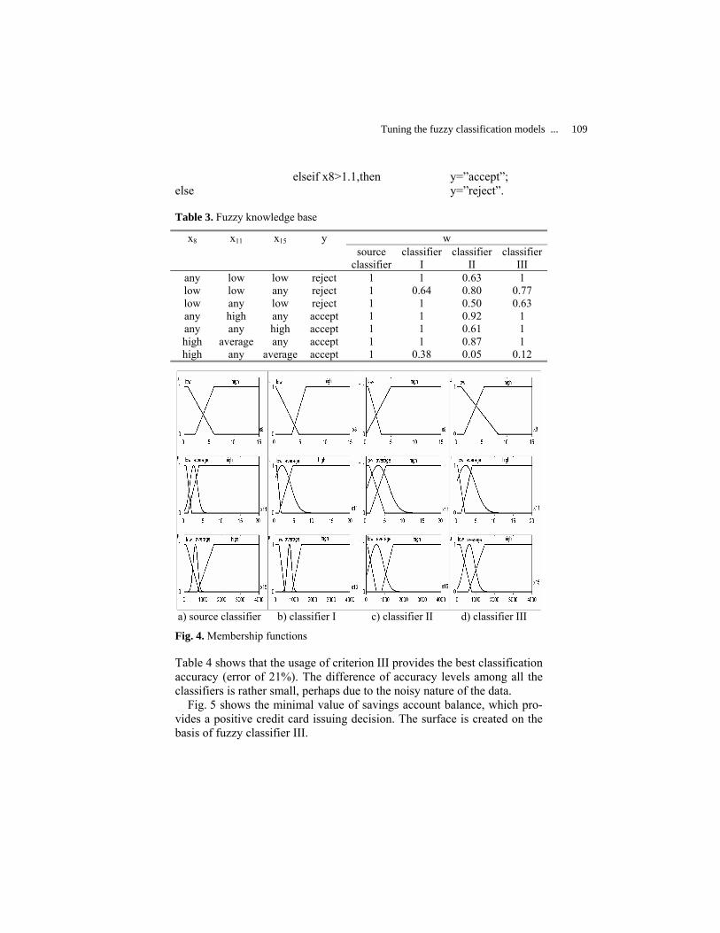
elseif x8>1.1,then y=”accept”; else y=”reject”.

Table 3. Fuzzy knowledge base

w x8 x11 x15 y source

classifierclassifier

I classifier

II classifier

III any low low reject 1 1 0.63 1 low low any reject 1 0.64 0.80 0.77 low any low reject 1 1 0.50 0.63 any high any accept 1 1 0.92 1 any any high accept 1 1 0.61 1 high average any accept 1 1 0.87 1 high any average accept 1 0.38 0.05 0.12

a) source classifier b) classifier I c) classifier II d) classifier III

Fig. 4. Membership functions

Table 4 shows that the usage of criterion III provides the best classification accuracy (error of 21%). The difference of accuracy levels among all the classifiers is rather small, perhaps due to the noisy nature of the data.

Fig. 5 shows the minimal value of savings account balance, which pro-vides a positive credit card issuing decision. The surface is created on the basis of fuzzy classifier III.


Table 4. Testing the classification models

Model Crite- rion I

Crite- rion II

Crite- rion III(R=4)

Misclas- sificationon test set

Source classifier 23.88% 0.46 2.34 23.5% Classifier I 23.47% 0.43 2.16 22.0% Classifier II 23.27% 0.35 1.49 22.5% Classifier III 23.88% 0.42 2.00 21.0% Decision tree 21.43% n/a n/a 22.5%

Fig. 5. Minimal value of the saving account for receiving a positive credit decision

5 Conclusion

We have studied three learning criteria for the tuning of a fuzzy classifier: 1) percentage of misclassification, 2) mean squared memberships’ differ-ence, and 3) penalized mean squared memberships’ difference. The abo-vementioned criteria were tested in 2 classification tasks: (a) a simple clas-sification problem with nonlinear separating curves and (b) a real credit-risk assessment problem. The experiments suggest that the third criterion provides the best classification accuracy, especially in the case of crisp separating curves. This allows us to recommend the penalized mean squared memberships’ difference, as a learning criterion of choice, for the proper tuning of fuzzy rule-based classification systems.

References

1. Rotshtein A (1998) Design and Tuning of Fuzzy Rule-Based Systems for Medical Diagnosis. In: Teodorescu NH, Kandel A, Jain LC (eds) Fuzzy and Neuro-Fuzzy Systems in Medicine. CRC-Press, Boca-Raton, pp 243-289

2. Sample Data Sets for the See5-Demo Product, Release 1.09a (2000). www.rulequest.com

3. Zimmermann H-J (1996) Fuzzy Set Theory and its Applications, 3rd ed.. Kluwer Academic Publishers, Norwell, Dordrecht

4. Zopounidis C, Pardalos PM, Baourakis G (eds., 2001) Fuzzy Sets in Management, Economics and Marketing. World Scientific, Singapore


prInvestor: Pattern Recognition basedFinancial Time Series Investment System

Dymitr Ruta1

BT Exact Technologies, Adastral Park, Orion Building, 1st floor - pp12,Martlesham Heath, Ipswich IP5 3RE, UK, [email protected]

ABSTRACTPredictability of financial time series (FTS) is a well-known dilemma. A typ-ical approach to this problem is to apply a regression model, built on thehistorical data and then further extend it into the future. If however thegoal is to support or even make investment decisions, regression-based FTSpredictions are inappropriate as on top of being uncertain and unnecessarilycomplex, they require further analysis to make an investment decision. Ratherthan precise FTS prediction, a busy investor may prefer a simple decision onthe current day transaction: buy, wait, sell, that would maximise his returnon investment. Based on such assumptions a classification model is proposedthat learns the transaction patterns from optimally labelled historical dataand accordingly gives the profit-driven decision for the current day transac-tion. Exploiting a stochastic nature of an investment cycle the model is locallyreduced to a 2-class classification problem and is built on many features ex-tracted from the share price and transaction volume time series. Simulation ofthe model over 20 years of NYSE:CSC share price history showed substantialimprovement of the profit compared to a passive long-term investment.

KEY WORDS

Financial Time Series, Regression, Classification, Decision Support

1 Introduction

Prediction of the financial time series represents a very challenging signal pro-cessing problem. Many scientist consider FTS as very noisy, non-stationaryand non-linear signal but believe that it is at least to a certain degreepredictable [3], [6]. Other analysis suggest that a financial market is self-guarded against predictability as whenever it shows some signs of apparentpredictability, investors immediately attempt to exploit the trading oppor-tunities, thereby affecting the series and turning it unpredictable [2]. Stable

forecasting of FTS seems therefore unlikely to persist for longer periods oftime and will self-destruct when discovered by a large number of investors.The only prediction model that could be successful and sustainable seems tobe the one that exploits the supportive evidence either hidden to other in-vestors or the evidence that is available but highly dispersed among manysources and therefore considered irrelevant, too difficult or too costly to beincorporated in the prediction model.

Irrespective of the above a number of techniques is being developed in anattempt to predict what seems unpredictable: tomorrow’s share price basedon historical data. Starting from simple linear Autoregressive Moving Averagemodels (ARMA) [3] through conditional heteroscedastic models like ARCHor GARCH [3] up to the complex non-linear models [3], [4], the idea is simi-lar: establish the regression-based description of the future samples based onthe historical data series. More recently a number of machine learning tech-niques started to be applied to a financial forecasting and on a number ofoccasions showed considerable improvement compared to a traditional regres-sion models [5], [6], [7]. Neural networks are shown to be particularly good atcapturing complex non-linear characteristics of FTS [5], [6]. Support vectormachines represent another powerful regression technique that immediatelyfound applications in financial forecasting [8], [7].

While there is already extensive knowledge available in pattern recognitiondomain, it has been rarely used for FTS prediction. The major problem liesin the fact that classification model learns to categorise patterns into crispclasses, rather than numerical values of the series. A temporal classificationmodels would have to provide a specific definition of classes or obtain it fromthe series by discretisation. Although some work has already been done in thisfield [10], [9], [11], [13] there is still lack of pattern recognition based modelsthat would offer immediate investment applications surpassing in functionalityand performance the traditional regression based models.

The proposed prInvestor model is a step forward towards a fully auto-mated pattern recognition based investment system. Rather than predictingfuture series values it uses a classification model that learns from expandablehistorical evidence how to automatically categorise the future series into in-vestment actions: buy, wait or sell. The prototype of prInvestor is tested onthe 20-years of daily share price series and the results are analysed to giverecommendations towards prospective fully automated platform development.

The remainder of the paper is organised as follows. Next section providesa detailed analysis of the proposed temporal classification with prInvestor,specifying the investment cycle, an algorithm for optimal labelling of trainingdata, feature extraction process and the classification model used. Section 3presents the results of extensive experiments with a real 20-year share pricedata series evaluating the performance of the prInvestor system. The con-cluding remarks and some suggestions for model refinement are shown in theclosing Section 4.

112 Ruta Dymitr

2 Temporal classification with prInvestor

Classification represents a supervised learning technique that tries to correctlylabel the patterns based on multidimensional set of features [1]. The model isfully built in the training process carried out on the labelled dataset with adiscriminative set of features. Based on the knowledge gained from the trainingprocess, a classifier assigns the label to a new previously unseen pattern.

Adapting the pattern recognition methodology, prInvestor would have togenerate the action label: buy, sell or wait to the current day feature valuesbased on the knowledge learnt from historical data. For that to be possiblethe training data have to be optimally labelled such that the investmentscorresponding to the sequence of labels generate the maximum return possible.Furthermore, to maximise the discrimination among classes, prInvestor shouldexploit the scalability of pattern recognition models and use as many relevantfeatures as possible, far beyond just the historical share price series. All theproperties mentioned above along with some mechanisms controlling modelflexibility and adaptability are addressed in the presented prInvestor system.

2.1 Investment cycle

In the simplified investment cycle, considered in this paper, the investor is us-ing all assets during each transaction which means he buys shares using all theavailable cash and sells all shares at once. Assuming this simplification, thereare four different states an investor can fall into during the investment cycle.He enters the cycle at the state ”wait with money” (WM), where the investoris assumed to possess financial assets and is holding on in the preparationfor a ”good buy”. From there he can either wait at the same state WM orpurchase the shares at the actual price of the day thereby entering the ”buy”state (B). From state B investor can progress to two different states. Either heenters ”wait with shares” state (WS) preparing for the good selling moment,or he sells immediately (the day after the purchase) all the shares transferringthem back to money at the ”Sell” (S) state. If the investor chooses to waitwith shares (WS), he can stay at this state or may progress only to the stateS. The sell state has to be followed by either the starting ”wait with money”state WM or directly buy state (B) that both launch the new investment cy-cle. The complete investment cycle is summarised by the conceptual diagramand accompanied directed cyclic graph both shown in Figure 1.

Immediate consequence of the investment cycle is that the labelling se-quence is highly constrained by the allowed transaction paths i.e. obeying thefollowing sequentiality rules:

• WM may follow only with WM or B• B may follow only with WS or S• WS may follow only with WS or S• S may follow only with WM or B

prInvestor: Pattern Recognition based Financial Time Series Investment System 113

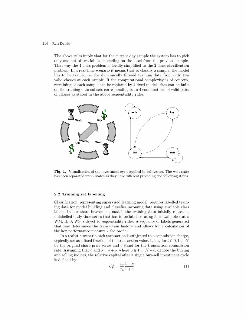
The above rules imply that for the current day sample the system has to pickonly one out of two labels depending on the label from the previous sample.That way the 4-class problem is locally simplified to the 2-class classificationproblem. In a real-time scenario it means that to classify a sample, the modelhas to be trained on the dynamically filtered training data from only twovalid classes at each sample. If the computational complexity is of concern,retraining at each sample can be replaced by 4 fixed models that can be builton the training data subsets corresponding to to 4 combinations of valid pairsof classes as stated in the above sequentiality rules.

Fig. 1. Visualisation of the investment cycle applied in prInvestor. The wait statehas been separated into 2 states as they have different preceding and following states.

2.2 Training set labelling

Classification, representing supervised learning model, requires labelled train-ing data for model building and classifies incoming data using available classlabels. In our share investment model, the training data initially representunlabelled daily time series that has to be labelled using four available statesWM, B, S, WS, subject to sequentiality rules. A sequence of labels generatedthat way determines the transaction history and allows for a calculation ofthe key performance measure - the profit.

In a realistic scenario each transaction is subjected to a commission charge,typically set as a fixed fraction of the transaction value. Let xt for t ∈ 0, 1, .., Nbe the original share price series and c stand for the transaction commissionrate. Assuming that b and s = b + p, where p ∈ 1, .., N − b, denote the buyingand selling indices, the relative capital after a single buy-sell investment cycleis defined by:

Csb =

xs

xb

1 − c

1 + c(1)

114 Ruta Dymitr

Note that the same equation would hold if the relative capital was calculatedin numbers of shares resulting from a sell-buy transaction. Assuming thatthere are T cycles in the series let b(j) and s(j) for j = 1, .., T denote indicesof buying and selling at jth cycle such that xb(j) and xs(j) stand for buy and

sell prices in jth cycle. Then the relative capital after k cycles (0 < k ≤ T )can be easily calculated by:

Cs(k)b(1) =

k∏j=1

Cs(j)b(j) (2)

The overall performance measure related to the whole series would be then theclosing relative capital, which means the relative capital after T transactions:

CT = Cs(T )b(1) (3)

Given CT the absolute value of the closing profit can be calculated by:

P = C0(CT − 1) (4)

where C0 represents the absolute value of the starting capital. Finally, tobe consistent with the investment terminology one can devise the return oninvestment performance measure, which is an annual average profit related toinitial investment capital:

R =PANN

C0=

[C

s(T )b(1)

] tANNs(T )−b(1) − 1 (5)

where tANN stands for the average number of samples in 12 months.The objective of the model is to deliver an optimal sequence of labels,

which means the labels that through the corresponding investment cyclesgenerate the highest possible profit. Such optimal labelling is only possibleif at the actual sample to be labelled, the knowledge of the future samples(prices) is available. Although reasoning from the future events is forbiddenin the realistic scenario, there is no harm of applying it to the training dataseries. The classification model would then have to try to learn the optimallabelling from historical data and use this knowledge for classification of newpreviously unseen samples.

An original optimal labelling algorithm is here proposed. The algorithm isscanning the sequence of prices and subsequently finds the best buy and sellindices labelling the corresponding samples with B and S labels respectively.Then all the samples in between of B and S labels are labelled with WS labeland all the samples in between of S and B labels are labelled with WM label asrequired by the sequentiality rules. The following rules are used to determinewhether the scanned sample is identified as optimal buy or sell label:

• Sample xb is classified with the label B (optimal buy) if for all samplesxt (b < t < s) between sample xb and the nearest future sample xs b, s ∈


1, .., N ∩ b < s, at which the shares would be sold with a profit (Csb > 1),

the capital Cst < Cs

b .• Sample xs is classified with the label S (optimal sell) if for all samples xt

(s < t < b) between sample xs and the nearest future sample xb b, s ∈1, .., N ∩s < b, at which the shares would be bought increasing the originalnumber of shares (Cs

b > 1), the capital Ctb < Cs

b .

2.3 Feature extraction

The data in its original form represents only a share price time series. Exten-sive research dedicated to time series prediction [3] proves that building themodel solely on the basis of historical data of the FTS is very uncertain asit exhibits considerable proportion of a random crawl. At the same time anattractive property of classification systems is that in most of the cases theyare scalable, which means they can process large number of features in a non-conflicting complementary learning process [1]. Making use of these attributes,prInvestor takes the original share price series, the average transaction volumeseries as well as the label series as the basis for the feature generation process.Details of the family of features used in prInvestor model are listed in Table1. Apart from a typical moving average, defferencing features, there are newfeatures (plf , ppf) that exploit the labels of past samples in their definition.The use of labels as features might draw some controversies as it imposes thatcurrent model outputs depend on its previous outputs. This is however truly areflection of the fact that investment actions strongly depend on the previousactions as for example if a good buy moment was missed the following good sellpoint could no longer be good. Incorporation of the dependency on previoussystem outputs (labels) injects also a needed element of the flexibility to themodel such that after a wrong decision, it could quickly recover rather thanmake further losses. Another consequence of using past labels as features isthe high non-linearity and indeterminism of the model and hence its limitedpredictability.

It is important to note that the features proposed in prototype of theprInvestor model are just a proposition of simple, cheap and available featureswhich by no means form the optimal set of features. In fact as the series is timerelated, countless number of features starting from the company’s P/E ratio oreconomy strength indicators up to type of weather outside or the investmentmood could be incorporated. The problem of generation and selection of themost efficient features related to the prInvestor model is by far open and willbe considered in more detail in the later version of prInvestor.

2.4 Classification model

Given the set of features, labelled training set and the performance measure,the model needs only a relevant classifier that could learn to label the samplesbased on optimal labels and the corresponding historical features available in

116 Ruta Dymitr

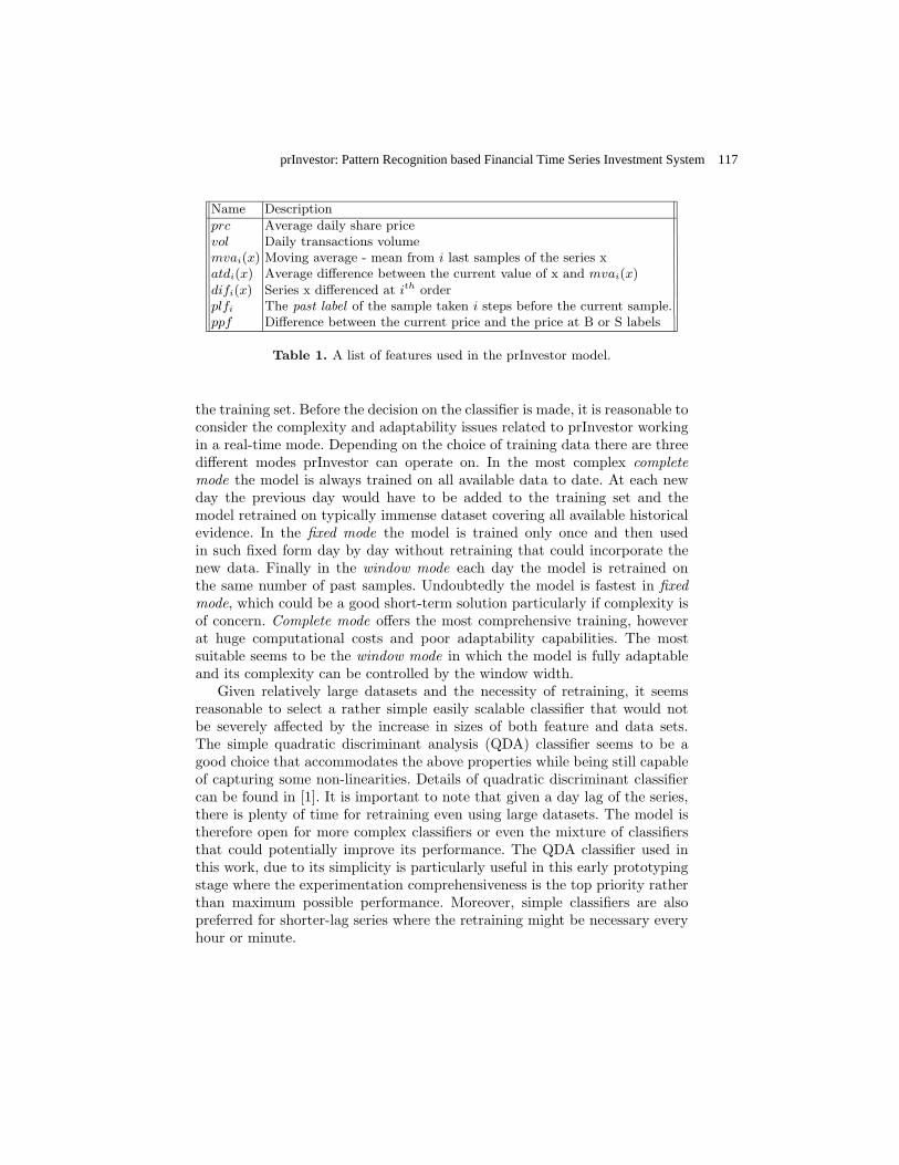
Name Description

prc Average daily share pricevol Daily transactions volumemvai(x) Moving average - mean from i last samples of the series xatdi(x) Average difference between the current value of x and mvai(x)

difi(x) Series x differenced at ith orderplfi The past label of the sample taken i steps before the current sample.ppf Difference between the current price and the price at B or S labels

Table 1. A list of features used in the prInvestor model.

the training set. Before the decision on the classifier is made, it is reasonable toconsider the complexity and adaptability issues related to prInvestor workingin a real-time mode. Depending on the choice of training data there are threedifferent modes prInvestor can operate on. In the most complex completemode the model is always trained on all available data to date. At each newday the previous day would have to be added to the training set and themodel retrained on typically immense dataset covering all available historicalevidence. In the fixed mode the model is trained only once and then usedin such fixed form day by day without retraining that could incorporate thenew data. Finally in the window mode each day the model is retrained onthe same number of past samples. Undoubtedly the model is fastest in fixedmode, which could be a good short-term solution particularly if complexity isof concern. Complete mode offers the most comprehensive training, howeverat huge computational costs and poor adaptability capabilities. The mostsuitable seems to be the window mode in which the model is fully adaptableand its complexity can be controlled by the window width.

Given relatively large datasets and the necessity of retraining, it seemsreasonable to select a rather simple easily scalable classifier that would notbe severely affected by the increase in sizes of both feature and data sets.The simple quadratic discriminant analysis (QDA) classifier seems to be agood choice that accommodates the above properties while being still capableof capturing some non-linearities. Details of quadratic discriminant classifiercan be found in [1]. It is important to note that given a day lag of the series,there is plenty of time for retraining even using large datasets. The model istherefore open for more complex classifiers or even the mixture of classifiersthat could potentially improve its performance. The QDA classifier used inthis work, due to its simplicity is particularly useful in this early prototypingstage where the experimentation comprehensiveness is the top priority ratherthan maximum possible performance. Moreover, simple classifiers are alsopreferred for shorter-lag series where the retraining might be necessary everyhour or minute.


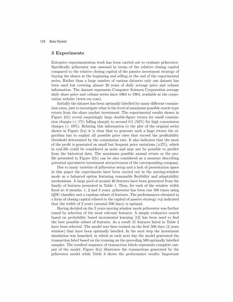
3 Experiments

Extensive experimentation work has been carried out to evaluate prInvestor.Specifically prInvestor was assessed in terms of the relative closing capitalcompared to the relative closing capital of the passive investment strategy ofbuying the shares at the beginning and selling at the end of the experimentalseries. Rather than a large number of various datasets only one dataset hasbeen used but covering almost 20 years of daily average price and volumeinformation. The dataset represents Computer Sciences Corporation averagedaily share price and volume series since 1964 to 1984, available at the corpo-ration website (www.csc.com).

Initially the dataset has been optimally labelled for many different commis-sion rates, just to investigate what is the level of maximum possible oracle-typereturn from the share market investment. The experimental results shown inFigure 2(b) reveal surprisingly large double-figure return for small commis-sion charges (< 1%) falling sharply to around 0.5 (50%) for high commissioncharges (> 10%). Relating this information to the plot of the original seriesshown in Figure 2(a) it is clear that to generate such a huge return the al-gorithm has to exploit all possible price rises that exceed the profitabilitythreshold determined by the commission rate. It also indicates that the mostof the profit is generated on small but frequent price variations (±2%), whichin real-life could be considered as noise and may not be possible to predictfrom the historical data. The maximum possible annual return or the pro-file presented in Figure 2(b) can be also considered as a measure describingpotential speculative investment attractiveness of the corresponding company.

Due to many varieties of prInvestor setup and a lack of presentation spacein this paper the experiments have been carried out in the moving-windowmode as a balanced option featuring reasonable flexibility and adaptabilitymechanisms. A large pool of around 40 features have been generated from thefamily of features presented in Table 1. Then, for each of the window widthfixed at: 6 months, 1, 2 and 3 years, prInvestor has been run 100 times usingQDC classifier and a random subset of features. The performances obtained ina form of closing capital related to the capital of passive strategy rcp indicatedthat the width of 2 years (around 500 days) is optimal.

Having decided on the 2 years moving window mode prInvestor was furthertuned by selection of the most relevant features. A simple evaluative searchbased on probability based incremental learning [12] has been used to findthe best possible subset of features. As a result 21 features listed in Table 2have been selected. The model was then trained on the first 500 days (2 yearswindow) that have been optimally labelled. In the next step the investmentsimulation was launched, in which at each next day the model generated thetransaction label based on the training on the preceding 500 optimally labelledsamples. The resulted sequence of transaction labels represents complete out-put of the model. Figure 3(a) illustrates the transactions generated by theprInvestor model while Table 3 shows the performance results. Important

118 Ruta Dymitr

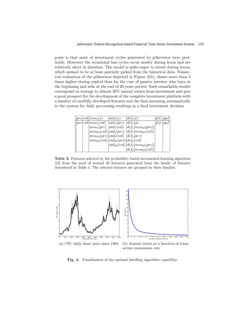
point is that most of investment cycles generated by prInvestor were prof-itable. Moreover the occasional loss cycles occur mostly during bessa and arerelatively short in duration. The model is quite eager to invest during hossa,which seemed to be at least partially picked from the historical data. Numer-ical evaluation of the prInvestor depicted in Figure 3(b), shows more than 5times higher closing capital than for the case of passive investor who buys atthe beginning and sells at the end of 20 years period. Such remarkable resultscorrespond on average to almost 20% annual return from investment and givea good prospect for the development of the complete investment platform witha number of carefully developed features and the data incoming automaticallyto the system for daily processing resulting in a final investment decision.

prc vol mvai(x) atdi(x) difi(x) plfi ppf

prc vol mva1(vol) atd1(prc) dif1(p) plf1 ppfmva5(prc) atd1(vol) dif1[mva20(prc)]mva20(vol) atd5(prc) dif1[mva20(vol)]mva50(prc) atd5(vol) dif2(prc)mva50(vol) atd20(prc) dif2(vol)

atd20(vol) dif2[mva20(prc)]

dif2[mva20(vol)]

Table 2. Features selected by the probability based incremental learning algorithm[12] from the pool of around 40 featured generated from the family of featuresintroduced in Table 1. The selected features are grouped by their families.

0 500 1000 1500 2000 2500 3000 3500 4000 4500 50000

1

2

3

4

5

6

working days since 1964

CS

C s

hare

pric

e [$

]

(a) CSC daily share price since 1964

0 2 4 6 8 10 12 14 16 18 200

2

4

6

8

10

12

14

16

18

20

22

transaction commission rate [%]

annu

al r

etur

n

(b) Annual return as a function of trans-action commission rate

Fig. 2. Visualisation of the optimal labelling algorithm capability.


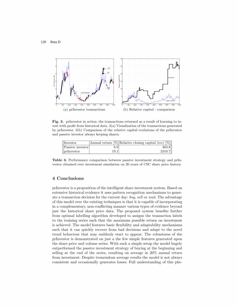
0 500 1000 1500 2000 2500 3000 3500 4000 45000

1

2

3

4

5

6

CS

C s

hare

pric

e [$

]

buy

sell

loss transaction

(a) prInvestor transactions

0 500 1000 1500 2000 2500 3000 3500 4000 45000

5

10

15

20

25

30

Rel

ativ

e ca

pita

l [C

/C0]

prInvestor

passive investor

(b) Relative capital - comparison

Fig. 3. prInvestor in action: the transactions returned as a result of learning to in-vest with profit from historical data. 3(a) Visualisation of the transactions generatedby prInvestor. 3(b) Comparison of the relative capital evolutions of the prInvestorand passive investor always keeping shares.

Investor Annual return [%] Relative closing capital (rcc) [%]

Passive investor 8.9 463.8prInvestor 19.1 2310.7

Table 3. Performance comparison between passive investment strategy and prIn-vestor obtained over investment simulation on 20 years of CSC share price history.

4 Conclusions

prInvestor is a proposition of the intelligent share investment system. Based onextensive historical evidence it uses pattern recognition mechanisms to gener-ate a transaction decision for the current day: buy, sell or wait. The advantageof this model over the existing techniques is that it is capable of incorporatingin a complementary, non-conflicting manner various types of evidence beyondjust the historical share price data. The proposed system benefits furtherfrom optimal labelling algorithm developed to assigns the transaction labelsto the training series such that the maximum possible return on investmentis achieved. The model features basic flexibility and adaptability mechanismssuch that it can quickly recover from bad decisions and adapt to the noveltrend behaviour that may suddenly start to appear. The robustness of theprInvestor is demonstrated on just a the few simple features generated uponthe share price and volume series. With such a simple setup the model hugelyoutperformed the passive investment strategy of buying at the beginning andselling at the end of the series, resulting on average in 20% annual returnfrom investment. Despite tremendous average results the model is not alwaysconsistent and occasionally generates losses. Full understanding of this phe-

120 Ruta D

nomenon requires deeper analysis of the role of each individual feature inthe decision process. In addition there is plenty of unknowns relating to thechoice of features, classifier and the real-time classification mode. All theseproblems and doubts will be the subject of further investigation towards fullyautomated and robust investment system that could potentially find somecommercial applications. For that to happen the system would have to meetvery restrictive reliability requirements confirmed by the extensive testingacross different company shares, markets, and time.

References

1. Duda RO, Hart PE, Stork DG (2001) Pattern classification. John Wiley &Sons. New York

2. Timmermann A, Granger CWJ (2004) Efficient market hypothesis and fore-casting. International Journal of Forecasting 20(1): 15-27(13)

3. Tsai RS (2002) Analysis of financial time series. John Wiley & Sons4. Casdagli M (1989) Nonlinear prediction of chaotic time series. Physica 35: 335-

3565. Vojinovic Z, Kecman V, Seidel R (2001) A data mining approach to finan-

cial time series modelling and forecasting. International Journal of IntelligentSystems in Accounting, Finance & Management 10(4): 225-239(15)

6. Giles CL, Lawrence S, Tsoi AC.(2001) Noisy time series prediction using re-current neural networks and grammatical inference. Machine Learning 44(1/2):161-183(23)

7. Tay FEH, Cao LJ (2002) Modified support vector machines in financial timeseries forecasting. Neurocomputing 48(1): 847-861(15)

8. Mukherjee S, Osuna E, Girosi F (1997). Nonlinear prediction of chaotic timeseries using support vector machines. In Proceedings of the 7th IEEE Workshopon Neural Networks for Signal Proc., IEEE Press

9. Singh S (2000) Noisy time-series prediction using pattern recognition tech-niques. Computational Intelligence 16(1): 114-133(20)

10. Morik K, Rueping S (2002) A multistrategy approach to the classification ofphases in business cycles. In Taprio E, Mannila H, Toivonen H (eds) LectureNotes in Artificial Intelligence (Machine Learning ECML 2002), pp. 307-318,Springer-Verlag

11. Wu B, Hung S-L (1999) A fuzzy identification procedure for nonlinear timeseries: With example on ARCH and bilinear models. Fuzzy Sets and Systems108(3): 275-287(13)

12. Ruta D, Gabrys B. Application of the evolutionary algorithms for classifierselection in multiple classifier systems with majority voting. In Proceedings ofthe 2nd International Workshop on Multiple Classifier Systems, LNCS 2096, pp399-408 Springer Verlag

13. Siekmann S, Neuneier R, Zimmermann H-G, Kruse R (1999) Neuro fuzzy sys-tems for data analysis. In Computing with Words in Zadeh LA, Kacprzyk J(eds) Information/Intelligent Systems Applications (Studies in Fuzziness & SoftComputing, Springer-Verlag


On general scheme of invariant clustering procedures based on fuzzy similarity relation

Batyrshin1,2 I.Z., Rudas3 T. , Klimova4 A.

1Mexican Petroleum Institute, Mexico 2Institute of Problems of Informatics, Academy of Sciences of Tatarstan, Russia 3 TARKI, Social Research Center, Hungary 4Kazan State Technological University, Russia [email protected], [email protected]

Abstract. We study the properties of general scheme of parametric invariant clustering procedures based on transformation of proximity function into fuzzy equivalence relation. The scheme gives possibility to build clustering procedures invariant to numeration of objects and to monotone transformation of proximity values between objects. The work of clustering procedure is demonstrated on example of clusterization of world stock markets.

1. Introduction

The requirements of invariance of clustering procedures under monotone transformations of similarity values between objects and invariance under permutation of objects are considered in cluster analysis as most important requirements on clustering algorithms [1, 6, 7]. The first requirement is necessary if similarity values are measured by experts or may be evaluated only in ordinal scale. This requirement is desirable also for insensitivity of clustering results to a choice of similarity or dissimilarity measure. The second requirement is necessary if we want to get as result of clustering procedure an intrinsic similarity structure of data independent on numeration of objects.

Different approaches to construction of invariant hierarchical clustering algorithms were considered in literature but only a few known algorithms fulfill to both requirements. One of such algorithms is single linkage algorithm discussed in many papers. This algorithm builds chains of clusters and for this reason reflects only specific point of view on “cluster” which is not always

acceptable. Nevertheless, this algorithm is considered as one of the most important clustering algorithm [7].

The scheme of clustering procedures discussed in this paper gives possibility to construct parametric clustering procedures invariant with respect to both invariance properties considered above.

In Section 2 we discuss the structure of clustering scheme and study its properties. In Section 3 we demonstrate the work of proposed clustering procedure on example of clusterization of world stock markets. In Conclusion we discuss obtained results.

2. General scheme of clustering algorithms

A valued relation on the set of objects X is a function S:X×X→R, where

R= [0,I] and I is some positive real value [5,10]. S called a similarity relation if it is reflexive: S(x,x) = I and symmetric: S(x,y)=S(y,x) on X. Linear ordering relation ≤ on R defines operations min and max denoted as ∧ and ∨ respectively: a∧b = a if a≤ b and a∧b = b if b≤ a; a∨b = b if a ≤ b and a∨b = a if b ≤ a. Similarity relation satisfying on X the property of (∨,∧)-transitivity: S(x,y)≥ min(S(x,z),S(z,y) will be called a valued equivalence relation.

For any value (level) a from R a valued relation S defines a usual relation S[a] and valued relation Sa as follows: S[a] = (x,y)∈XS(x,y) ≥ a; Sa(x,y) = 1, if S(x,y) ≥ a and Sa(x,y) = 0, if S(x,y) < a. Valued relation Sa may be considered as characteristic function of usual relation S[a]. From a < b it follows that S[b] ⊆ S[a] and Sb ⊆ Sa. From reflexivity and symmetry of S it follows that for all a∈R the usual relations S[a] also will be reflexive and symmetric. If S is (∨,∧) - transitive then all S[a] will be transitive relations [10]. As result, valued equivalence relation defines the nested set of usual equivalence relations and hence the nested partition of X on equivalence classes.

The subset A of X will be called a similarity class of similarity relation S on X if S(x,y) > S(x,z) for all x,y ∈A and all z∉A. A similarity class A may be considered as natural cluster in the set X.

Proposition 1. A set of similarity classes of a valued equivalence relation S coincides with a set of equivalence classes of relations S[a], a∈R.

The following scheme of clustering algorithms was proposed in [1]:

E = Q(S) = TC(F(S))=∧

)(SF ,

On general scheme of invariant clustering procedures based on fuzzy similarity relation 123

where F is some “correction” of given similarity relation S such that F(S) ⊆ S and TC denotes the procedure of transitive closure ^ of valued similarity relations [8, 10]. The procedure of transitive closure may be realized by single linkage algorithm [4]. This procedure has both types of invariance. Hence, if correction procedure F also have both types of invariance then the clustering procedure Q will satisfy to desirable properties of invariance.

The correction procedure may be based on the following idea. Two objects x and y are considered as identical in S if S(x,y) = I and S(x,z) = S(y,z) for all objects z from X\x,y. More generally, two objects x and y will be called indistinguishable on the level a∈R if S(x,y) ≥ a and for any z∈ X it is fulfilled S(x,z) ≥ a if and only if S(y,z) ≥ a. It is clear that two objects indistinguishable on some level a will be identical in similarity relation Sa . It is clear also that all objects are indistinguishable on the minimal possible level 0 and the maximal possible level of indistinguishability of two objects x and y in relation S is equal to a = S(x,y). Two objects x and y indistinguishable on the level a = S(x,y) will be called indistinguishable in S.

Proposition 2. A similarity relation S defined on X will be a valued equivalence relation if and only if all objects of X are indistinguishable in S.

From the properties of the procedure of transitive closure TC it follows that it transforms any similarity relation S into valued equivalence relation E such that S ⊆ E and E is the minimal valued equivalence relation including S. Hence transitive closure procedure produces minimal increase of values S(x,y) for transformation S into valued equivalence relation E. From Proposition 2 we can conclude that this procedure transforms non-indistinguishable pairs of objects into indistinguishable. Hence we can suppose that the total value of transformation of S into E produced by TC depends on the number of non-indistinguishable pairs of elements in S and on the “degree of indistinguishability” of these elements, if we can measure this degree. Hence the correction procedure F decreasing similarity values S(x,y) should produce such minimal corrections of these values which will increase the number of indistinguishable pairs of objects or increase the “degree of indistinguishability” of pairs of objects. In this case the transformation TC(F(S)) produced by procedure of transitive closure will be small.

For construction of suitable correction procedure it is desirable to decide: for what pairs of objects (x,y) the similarity values S(x,y) should be corrected and how these values should be decreased. For these purposes the following evaluation of indistinguishability may be used. We will say that two objects x

124 Batyrshin I.Z., Rudas T. and Klimova A.

and y are indistinguishable with respect to object z when S(x,z) ≥ S(x,y) if and only if S(y,z)≥ S(x,y). In this case we will say that object z “support” similarity value S(x,y). The more the objects in X supporting similarity value S(x,y) the more the degree of indistinguishability of x and y. Our goal is to change the value of S(x,y) such that the number of objects supporting similarity between x and y and hence the degree of indistinguishability will increase. As result we can say that if the objects x and y are indistinguishable only with respect to small part of objects and hence they show different behavior on large part of objects then the similarity value S(x,y) does not confirmed or supported by objects of the set X and as result, the similarity value S(x,y) may be corrected (decreased).

The correction procedure based on these ideas will depends on the following sets and parameters:

Vy(x) = z∈X\x,y S(x,z) ≥ f1(S(x,y)), Vx(y) = z∈X\x,y S(y,z) ≥ f1(S(x,y)),

where f1:R→R is some function. The sets Vy(x) and Vx(y) denote the sets of objects “similar” to x and to y respectively when the value f1(S(x,y)) serves as criteria of this similarity. The set V(x,y) = z∈X\x,ymaxS(x,z),S(y,z) ≥ f2(S(x,y)), contains the objects from X which are “similar” at least to one of the objects x and y. When f1 ≡ f2 we have V(x,y)=Vy(x)∪Vx(y). This set will be considered as the set of “neighbors” of x and y. The “voices” of objects from V(x,y) will be taken into account when decision about correction of the value S(x,y) will be made. The following set W(x,y) = z∈X\x,y minS(x,z),S(y,z) ≥ f3(S(x,y)) denotes the set of “strong” or “common” neighbors, i.e. objects which are “similar” to both objects x and y. The objects from W(x,y) will “support” the value S(x,y). When f1 ≡ f3 we have W(x,y)= Vy(x)∩Vx(y).

The decision about correction of the value S(x,y) will depend on the respective part of objects “supporting” the similarity value S(x,y) which may be considered as measure of indistinguishability of objects x and y. We can consider the following methods of calculating for each pair of objects x and y this respective part denoted as hi:

hW x y

V x V yy x1 =

( , )

min( ( ) , ( ) ), h

W x y

V x V yy x2 =

( , )

max( ( ) , ( ) ) , h

W x y

V x y3 =

( , )

( , ),

where we set hi = 1 if denominator of hi is equal to 0. The correction procedure F(S) = Sc of clustering procedure Q may be

defined as follows:


≥

=elseyxF

phifyxSyxS

jc

i

),(

),(),( ,

where p∈[0,1] is a parameter and Fj(x,y) is a corrected value such that Fj(x,y)⊆ S(x,y). We will suppose that Fj(x,y) depends on the values S(x,z), S(y,z) of objects z belonging to the sets of neighbors of x and y: Vy(x), Vx(y) and V(x,y). It may be used some mean of this values. At least we require that Fj(x,y) ≥ minz∈VS(x,z),S(y,z), where V=Vy(x)∪Vx(y)∪V(x,y). The following functions showed good result on many experimental data: F1= min, F2= max, F3= mean. When p = 0, from hj ≥ 0 it follows that F(S(x,y))= Sc(x,y) =S(x,y), i.e. for all x,y from X the values S(x,y) will be not corrected and Q(S) = TC(F(S))=TC(S), i.e. clustering algorithm will coincide with single-linkage algorithm.

Proposition 3. For clustering procedures Q with identity functions f 1 - f3 it is fulfilled Q(S) = S if and only if S is a valued equivalence function.

One of the possible desirable properties of clustering algorithm is “to keep similarity classes”. Similarity classes satisfy to intuitively evident opinion about natural cluster. If such clusters exist in initially given similarity relation S then these clusters also should exist in clusterization obtained by clustering procedure. More generally we can require that if the subset A is a similarity class of any similarity relation S then A should be a similarity class of the valued equivalence relation E obtained by clustering procedure.

Proposition 4. Clustering procedure from proposed scheme “keeps similarity classes” if the functions f 1 and f 2 used in this procedure are identity functions.

Methods of clusterizations based on corrections procedures Fj with j= 1, 2 are invariant to monotone transformations of similarity values because they use only ordinal information about similarity values. Instead of method Fj with j=3 it may be used its ordinal extension when instead of mean of similarity values S(x,y),S(x,z) which are less than S(x,y) the median of these values or “k-th” similarity value chosen from ordered list of these values are used.

The experience of practical application of clustering procedures shows that these algorithms give good results for different data but for classification of some types of data these procedures may be modified. The use of non-identity functions f1 - f3 essentially extends the possibilities of proposed scheme. It may be used for construction clusters based on idea of “break bridges between clusters” [2,3]. This approach from some point of view is opposite to the approach “keep similarity classes” because this approach may


break the similarity clusters which may be considered as “bridges” between natural clusters.

Define dissimilarity measures as follows: D(x,y)=I - S(x,y), S(x,y)= I-D(x,y), where I is the maximal value of similarity or dissimilarity between object. Then the sets Vy(x), Vx(y), V(x,y) and W(x,y) will be defined as follows:

Vy(x) = z∈X\x,y D(x,z) ≤ f1(D(x,y)), Vx(y) = z∈X\x,y D(y,z) ≤ f1(D(x,y)), V(x,y) = z∈X\x,y min(D(x,z),D(y,z) ≤ f2(D(x,y)), W(x,y) = z∈X\x,y max(D(x,z),D(y,z) ≤ f3(D(x,y))

where f1 , f2 , f3:R→R are some functions. When the dissimilarities are measured in quantitative scale we can define the functions f i as follows: f i(D(x,y))=k i⋅D(x,y), for i = 1,2,3, where k i ∈[0,1] are some parameters. If dissimilarities are measured in ordinal scale then the values of fk(D(x,y)) may be chosen between the values of D(u,v), u,v∈X. These sets have a natural interpretation as the sets of objects located from one of objects x, y or from both of them on the distance no greater than the distance f i (D(x,y)).

The considered clustering procedures are based on the calculation of numbers of “strong neighbors” for all pairs of objects. These methods “keep the similarity values between indistinguishable objects”. But for non-indistinguishable pairs of objects even with minimal distances between them the strong neighbors may be absent and the similarity values between these objects will be not supported by onother objects and hence may be corrected. Sometimes this situation is desirable but sometimes it may be better to keep these similarity values by extending the set of strong neighbors. All similarity values between these objects and the nearest objects will be corrected because they do not supported by onother objects. In such cases the use of non-identity functions f3 such that D(x,y) ≤ f3(D(x,y)) will give possibility to increase the number of strong neighbors for nearest objects and hence does not to correct the similarity values between them. These strong neighbors may be chosen between neighbors of x and y belonging to V(x,y).

3. Example

To demonstrate the work of the clustering scheme it was applied to clusterization of World stock markets [9]. Distance measure was calculated based on information about these stock markets for 1996-2004 years. Table 1 shows the results of clusterization of these data by clustering procedure from


considered scheme. 24 stock markets were jointed in 4 clusters (A,B,C,D) and 11 constitute single objects (X) do not jointed in clusters with other objects. Cluster B contains only European stock markets, Cluster C contains only Asian stock markets, cluster D contain 2 country: Poland and Israel, cluster A is a mixture of stock markets from Asia and Europe.

Table 1. Clusterization of 35 world stock markets.

Class Country Stock Market Class Country Stock Market B Belgium BEL20 A Austria Trad B Denmark KFX A Norway Oslo All Share

B France Cac

A Czech Republic PX50

B Germany Dax A India BSE Sens B Ireland ISEQ A Indonesia Jakarta Comp B Italy Mibtel General A Japan Second section B Netherlands CBS All B Spain Madrid SE X Finland HEX General B Switzerland SMI X Portugal PSI General X Sweden All Share

D Israel Tel Aviv-100 X Turkey IMKB Nat 100 D Poland WIG X Hungary BUX X Russia RTS

C Hong Kong Hang Seng X China CLSA China B C Japan Nikkei 225 X Pakistan KSE-100 C Japan Topix X South Korea KOSPI C Malaysia KLSE Comp X Sri Lanka CSE All Shr C Philippines Manila Comp X Thailand Bangkok SET C Singapore Straits Times C Taiwan Weighted

Conclusions

The properties of general scheme of invariant clustering procedures was studied in this work. It was shown that procedures from this scheme are rational, i.e. keep similarity classes etc for wide class of functions used in this scheme. But this scheme may be also extended for construction clusters based on the idea “break bridges between clusters”. The example of clusterization of worlds stock markets by clustering procedure from this scheme is considered.


Acknowledgements

This work was supported in part by Research Fellowship Program of Open Society Institute, by IMP, projects D.00006 and by RFBR grants 02-01-00092 and 03-01-96245.

References

[1] Batyrshin I.Z., Shuster V.A. (1984). The structure of semantic spaces of verbal estimates of actions. Trans. AI, Principle Questions of Knowledge Theory, Acta et Comment. Univ. Tartuensis, Tartu, vol. 688, pp. 20-38 (in Russian).

[2] Batyrshin I., Rudas T. (2000) Invariant clustering procedures based on corrections of similarities. In: Proceedings of East West Fuzzy Colloquium, Zittau, Germany, pp. 302-309.

[3] Batyrshin I., Klimova A. (2002) New invariant relational clustering procedures, In: Proceedings of East West Fuzzy Colloquium, 0th Zittau Fuzzy Colloquium, Zittau, Germany, 2002, 264 – 269.

[4] Dunn J.C. (1974). A graph-theoretic analysis of pattern classification via Tamura's fuzzy relation. IEEE Trans. SMC, vol. SMC-4, pp. 310-313.

[5] Fodor J.C., Roubens M. (1995). Structure of transitive valued binary relations. Mathematical Social Sciences, vol. 30, pp. 71-94.

[6] Hubert L.J. (1973). Monotone invariant clustering procedures. Psychometrica, vol. 38, pp. 47-62.

[7] Jardine N. & Sibson R. (1971). Mathematical taxonomy. London: John Wiley & Sons.

[8] Tamura S., Higuchi S. & Tanaka K. (1971). Pattern classification based on fuzzy relations. IEEE Trans. SMC, vol. SMC-1, pp. 61-66.

[9] World stock market data base: http://www.countrybriefings.com [10] Zadeh L.A. (1973). Similarity relations and fuzzy orderings. Information

Sciences, vol. 3, pp. 177-200.


Evolutionary procedures of visualization of multidimensional data

Angelica Klimova

Kazan State Technological University, e-mail: [email protected]

ABSTRACT. The methods of two dimensional (2D) and three dimen-sional (3D) visualization of multidimensional data are considered. They are both based on a minimization of the average alteration of all distances between objects. For each of procedures to visualization it was developed a genetic algorithm for minimization of correspondent distance alterations. The structures of these algorithms are discussed. The results of application of both methods are illustrated on the example of visualization of world stock markets.

1. Introduction

A visualization of data gives usually an important information for un-derstanding a data structure. Such information about mutual spatial loca-tion of objects may be obtained by methods of data visualization represent-ing initial data set in two dimensional (2D) or three dimensional (3D) spaces [3]. For these purposes the principal component analysis and the multidimensional scaling are often used. The first method is based on a se-quential rotation of initial coordinate system such that the variance of data in the direction of each new axis becomes maximal. Data visualization is obtained as result of projection of data on hyper planes correspondent to the first two or three (principal) axis. But distances between objects in ini-tial n-dimensional space of attributes may essentially differ from distances in 2D or 3D space of principal components. Multidimensional scaling gives possibility to decrease the space dimension with maximal preserva-tion of initial distances between objects but a reduction of space dimension till 2 or 3 as usually causes valuable distance alteration.

The problem of data visualization may be considered as a problem of 2D (or 3D) representation of objects which minimizes alterations of initial distances between objects. Existing methods of optimization give as usu-ally a local optimum for this problem. The search of a global optimum

may be based on the use of a genetic algorithm of optimization [2]. The structure of such algorithm is considered here.

Two genetic algorithms of data visualization are proposed in this paper. Both of algorithms minimize the average distance alteration between all objects. The proposed algorithms are illustrated on example. In Section 2 the genetic algorithm of 2D visualization of data is proposed. The genetic algorithm of 3D visualization of data is described in Section 3.

2. Genetic algorithm for 2D visualization of data

Suppose R is a distance function between objects from M in n-dimensional space of attributes, n > 3. We are finding 2D representation of these objects. First, the initial matrix of coordinates of objects in 2D space with axis X and Y is generated. Based on this matrix by standard optimiza-tion procedure it is determined a matrix of coordinates P of objects with the minimal error of approximation of initial matrix D by a distance matrix R calculated for matrix of coordinates P. Usually the obtained solution gives a local optimum. Then two objects a and b from M with the maximal value R(a,b) are determined. The system of coordinate <X,Y> is moved and rotated so that its center is moved to the point a and the point b is lo-cated on axis X.

The rotation is realized by the following transformation. Suppose <X,Y> is the system of coordinate which we had before transformation but after moving and <X`,Y`> is the “new” system of coordinate. The direction of the axis X` is coincide with the direction of the vector with the begin-ning in the point a and with the end in the point b. Calculate the angle be-tween axis X and X` as following:

⎟⎟⎟⎟⎟

⎠

⎞

⎜⎜⎜⎜⎜

⎝

⎛−⋅

= 2

22

4arcsinx

bxb

b

RbRϕ

where Rb is the distance between point b in the “old” system of coordinate after moving and the point b in the “new” system of coordinate, bx is the coordinate of the point b in the “old” system of coordinate after moving. If the point b in the “old” system of coordinate after moving was in the I or III coordinate quarter then the angle of the rotation is equal -ϕ. If the point b in the “old” system of coordinate after moving was in the II or IV coor-dinate quarter then the angle of the rotation equals to ϕ.

Then define the matrix of the rotation like this:

Evolutionary procedures of visualization of multidimensional data 131

⎟⎟⎟⎟

⎠

⎞

⎜⎜⎜⎜

⎝

⎛

⎟⎠⎞

⎜⎝⎛ −

⎟⎠⎞

⎜⎝⎛ +

=ϕϕπ

ϕπϕ

cos2

cos

2coscos

rotM

And at last determinate the coordinates of objects in the “new ” system of coordinate <X`,Y`> : P*=MrotPT.

Then it is defined an object c with the maximal absolute value yc of co-ordinate Y in the matrix of coordinates obtained after rotation and dis-placement of coordinate system P. If yc < 0 then the sign of Y coordinates of all objects is changing on opposite. The objects a,b,c will be reference elements for all future coordinate matrixes. The obtained matrix of coordi-nates P* of objects from M is called a solution and an error of approxima-tion of matrix D by matrix of distances R calculated from P* is called an error of the solution.

Further it is randomly generated the set of m matrixes of initial coordi-nates of objects in 2D space and for each of them it is calculated the error of approximation. The obtained set of matrixes is called a population. The best q matrixes with minimal errors are selected from population and called elite.

For each matrix of coordinate from elite it is applied a shift and rotation of all coordinates in order to locate the reference elements a,b,c in similar positions as in the matrix P*. The obtained solutions are used further for generation of new solutions called descendants. They are obtained as result of application of the following steps. Couples of solutions (“parents”) are randomly selected from elite and used further for construction of new solu-tions “descendants”) by means of recombination and mutation operations defined as follows.

Recombination operation: It is randomly selected an object x from M and all objects from one of parents with the number less than number of x receive the coordinates of the same objects from another parent.

Mutation operation: The matrix of coordinates of solution is added with the matrix of normally distributed increments multiplied by some small value Q.

A new population is obtained as a union of old elite, descendants ob-tained after recombination, mutated old elite and mutated descendants. For new elements of elite defining the matrixes of coordinates of objects in 2D space they are calculated the correspondent distance matrixes and correspondent errors of approximation of initial matrix of distances in n-dimensional space.

From the obtained population new elite is selected as follows: half of the elite consists of the best solutions in population and half of the elite is ran-

132 Klimova Angelica

domly selected from population. For new elite they are applied all the steps considered above: shift and rotation of all coordinates, selection of parents and generation of descendants etc.

The generation of new populations is repeated a given number of times or it is stopped if it will be found a solution with the error less than given value.

Proposed genetic algorithm was applied for visualization of 15 objects given in 8-dimensional space. The coordinates of objects in this space were from World Stock Market Data Base [7] and presented in Table 1. This table allows to compare the performance of 15 markets over the last 8 years with 15 key indices. Prices are quoted in local currency, the MSCI index is in US dollars. The % change is based on the opening level of the index on the first of January each year, and then on the first of each month.

Table 1.

Asia 2003 2002 2001 2000 1999 1998 1997 1996 1 China 10.25 -28.7 29.32 130.5 226.9 77.27 50.76 162.2

2 Hong Hong 34.92 10.34 -16.7 -25.9 25.15 17.28 -4.75 24.84

3 India 72.89 78.98 47.00 16.64 91.10 59.58 81.04 87.72

4 Indo-nesia 62.82 76.49 66.19 2.21 73.83 72.24 8.43 34.65

5 Japan 24.45 1.27 -22.6 -43.6 -22.9 -30 -44.9 -46.3 6 Japan 23.76 1.12 -18.7 -39.4 -3.98 -11.2 -29 -33.9 7 Japan 43.93 25.52 10.38 -18.1 81.23 78.74 17.16 3.65

8 Malaysia 22.84 14.06 16.82 -2.26 35.45 33.56 -35.5 -20.2

9 Paki-stan 65.53 251.2 196.6 217.4 373.1 154.9 233.5 198.2

10 Phil-ippines 41.63 23.48 -3.49 -32.7 -26.7 -22.8 -54.3 -44.4

11 Sin-gapore 31.58 8.68 -8.42 -28.8 26.70 15.34 -20.4 -21.9

12 South Korea 29.19 16.87 60.66 -21.1 44.14 115.4 24.49 -8.18

13 Sri Lanka 30.34 71.07 137.4 85.58 77.86 51.29 76.18 67.65

14 Tai-wan 32.30 6.11 24.17 -30.3 -8.22 -28 -15 14.19

15 Thai-land 116.6 154.1 186.8 60.22 117 107.2 -3.86 -39.7

The optimal coordinates of objects in 2D space were found by standard procedure of approximation of nonlinear function by least squared method.


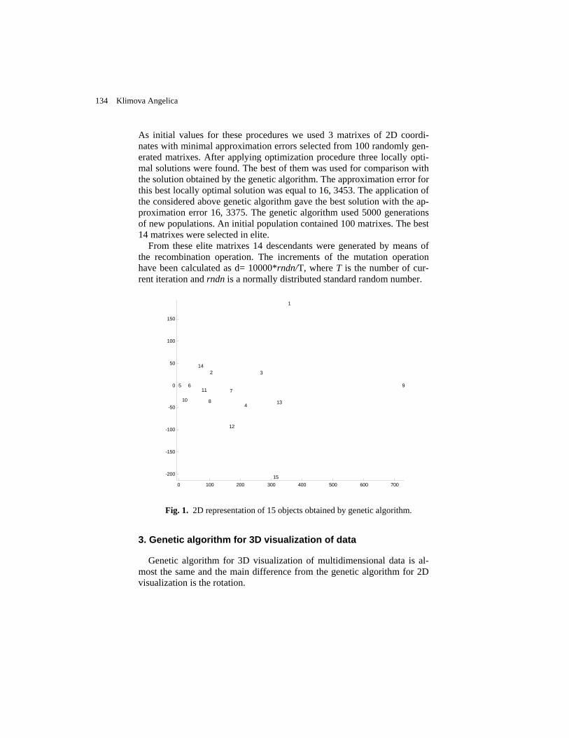
As initial values for these procedures we used 3 matrixes of 2D coordi-nates with minimal approximation errors selected from 100 randomly gen-erated matrixes. After applying optimization procedure three locally opti-mal solutions were found. The best of them was used for comparison with the solution obtained by the genetic algorithm. The approximation error for this best locally optimal solution was equal to 16, 3453. The application of the considered above genetic algorithm gave the best solution with the ap-proximation error 16, 3375. The genetic algorithm used 5000 generations of new populations. An initial population contained 100 matrixes. The best 14 matrixes were selected in elite.

From these elite matrixes 14 descendants were generated by means of the recombination operation. The increments of the mutation operation have been calculated as d= 10000*rndn/T, where T is the number of cur-rent iteration and rndn is a normally distributed standard random number.

0 100 200 300 400 500 600 700

-200

-150

-100

-50

0

50

100

150

1

2 3

4

5 67

8

9

10

11

12

13

14

15

Fig. 1. 2D representation of 15 objects obtained by genetic algorithm.

3. Genetic algorithm for 3D visualization of data

Genetic algorithm for 3D visualization of multidimensional data is al-most the same and the main difference from the genetic algorithm for 2D visualization is the rotation.


Suppose R is a distance function between objects from M in n-dimensional space of attributes, n > 3. We are finding 3D representation of these objects. First, the initial matrix of coordinates of objects in 3D space with axis X and Y is generated. Based on this matrix by standard optimiza-tion procedure it is determined a matrix of coordinates P of objects with the minimal error of approximation of initial matrix D by a distance matrix R calculated for matrix of coordinates P. Usually the obtained solution gives a local optimum. Then two objects a and b from M with the maximal value R(a,b) are determined. The system of coordinate <X,Y,Z> is moved and rotated such that it’s center is moved to the point a and the point b is located on axis X.

The rotation is realized by the following transformation. Suppose <X,Y> is the system of coordinate which we had before transformation but after moving and <X`,Y`> is the “new” coordinate system. The direction of the axis X` is coincided with the direction of the vector with the beginning in the point a and with the end in the point b. Assume (bx, by, bz) are coor-dinates of the point b before rotation and d is the distance between points a and b. In the system of coordinate <X,Y> defined coordinates of basis vectors of coordinate system <X`,Y`> (the direction of the vector 1er is co-incide with the direction of the vector with the beginning in the point a and with the end in the point b ):

,,,1 ⎟⎟⎠

⎞⎜⎜⎝

⎛=

db

db

db

e zyxr ,0,,

22222⎟⎟⎟

⎠

⎞

⎜⎜⎜

⎝

⎛

+

−

+=

yx

x

yx

y

bb

b

bb

ber

.,,22

22223⎟⎟⎟

⎠

⎞

⎜⎜⎜

⎝

⎛ +−

+⋅

⋅

+⋅

⋅=

d

bb

bbd

bb

bbd

bbe

yx

yx

zy

yx

zxr

Coordinates of basis vectors of coordinate system <X,Y> : ).1,0,0(),0,1,0(),0,0,1( === kji

rrr

The matrix of the rotation consists from the cosines of angles between vectors )3,2,1( =iei

r and kji

rrr,, :

⎟⎟⎟⎟⎟⎟⎟⎟⎟

⎠

⎞

⎜⎜⎜⎜⎜⎜⎜⎜⎜

⎝

⎛

+−

+⋅

⋅

+

−

+⋅

⋅

+

=

d

bb

db

bbd

bb

bb

bd

bbbd

bb

bb

bd

b

M

yxz

yx

zy

yx

xy

yx

zx

yx

yx

rot

22

2222

2222

0


Coordinates of objects are defined as following: P*=(MrotPT)T. Then it is defined an object c with the maximal absolute value yc of co-

ordinate Y in the matrix of coordinates obtained after rotation and dis-placement of coordinate system P. If yc < 0 then the sign of Y coordinates of all objects is changing on opposite. And then it is defined an object t with the maximal absolute value zt of coordinate Z in the matrix of coordi-nates obtained after rotation and displacement of coordinate system P. If zt< 0 then the sign of Z coordinates of all objects is changing on opposite. The objects a,b,c,t will be reference elements for all future coordinate ma-trixes. The obtained matrix of coordinates P* of objects from M is called a solution and an error of approximation of matrix D by matrix of distances R calculated from P* is called an error of the solution.

Further it is randomly generated the set of m matrixes of initial coordi-nates of objects in 3D space and for each of them it is calculated the error of approximation. The obtained set of matrixes is called a population. The best q matrixes with minimal errors are selected from population and called elite.

For each matrix of coordinates from elite it is applied a shift and rota-tion of all coordinates in order to locate the reference elements a,b,c,t in similar positions as in the matrix P*. The obtained solutions are used fur-ther for generation of new solutions called descendants. They are obtained as result of application of the following steps. Couples of solutions (“par-ents”) are randomly selected from elite and used further for construction of new solutions “descendants”) by means of recombination and mutation operations defined as follows.

Recombination operation: it is randomly selected an object x from M and all objects from one of parents with the number less than number of x receive the coordinates of the same objects from another parent.

Mutation operation: the matrix of coordinates of solution is added with the matrix of normally distributed increments multiplied by some small value Q.

A new population is obtained as a union of old elite, descendants ob-tained after recombination, mutated old elite and mutated descendants.

For new elements of elite defining the matrixes of coordinates of objects in 3D space they are calculated the correspondent distance matrixes and correspondent errors of approximation of initial matrix of distances in n-dimensional space.

From the obtained population it is selected new elite as follows: half of elite consists of the best solutions in population and half of elite is ran-domly selected from population. For new elite they are applied all the steps considered above: shift and rotation of all coordinates, selection of parents and generation of descendants etc.


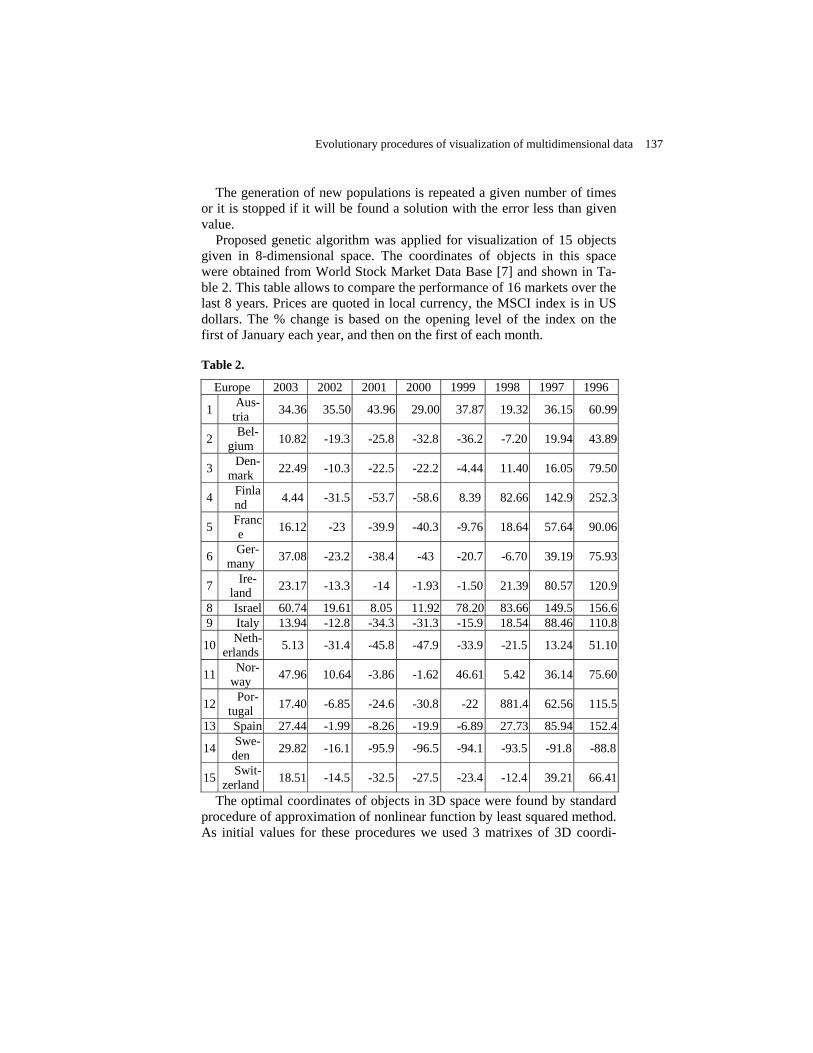
The generation of new populations is repeated a given number of times or it is stopped if it will be found a solution with the error less than given value.

Proposed genetic algorithm was applied for visualization of 15 objects given in 8-dimensional space. The coordinates of objects in this space were obtained from World Stock Market Data Base [7] and shown in Ta-ble 2. This table allows to compare the performance of 16 markets over the last 8 years. Prices are quoted in local currency, the MSCI index is in US dollars. The % change is based on the opening level of the index on the first of January each year, and then on the first of each month.

Table 2.

Europe 2003 2002 2001 2000 1999 1998 1997 1996

1 Aus-tria 34.36 35.50 43.96 29.00 37.87 19.32 36.15 60.99

2 Bel-gium 10.82 -19.3 -25.8 -32.8 -36.2 -7.20 19.94 43.89

3 Den-mark 22.49 -10.3 -22.5 -22.2 -4.44 11.40 16.05 79.50

4 Finland 4.44 -31.5 -53.7 -58.6 8.39 82.66 142.9 252.3

5 France 16.12 -23 -39.9 -40.3 -9.76 18.64 57.64 90.06

6 Ger-many 37.08 -23.2 -38.4 -43 -20.7 -6.70 39.19 75.93

7 Ire-land 23.17 -13.3 -14 -1.93 -1.50 21.39 80.57 120.9

8 Israel 60.74 19.61 8.05 11.92 78.20 83.66 149.5 156.6 9 Italy 13.94 -12.8 -34.3 -31.3 -15.9 18.54 88.46 110.8

10 Neth-erlands 5.13 -31.4 -45.8 -47.9 -33.9 -21.5 13.24 51.10

11 Nor-way 47.96 10.64 -3.86 -1.62 46.61 5.42 36.14 75.60

12 Por-tugal 17.40 -6.85 -24.6 -30.8 -22 881.4 62.56 115.5

13 Spain 27.44 -1.99 -8.26 -19.9 -6.89 27.73 85.94 152.4

14 Swe-den 29.82 -16.1 -95.9 -96.5 -94.1 -93.5 -91.8 -88.8

15 Swit-zerland 18.51 -14.5 -32.5 -27.5 -23.4 -12.4 39.21 66.41

The optimal coordinates of objects in 3D space were found by standard procedure of approximation of nonlinear function by least squared method. As initial values for these procedures we used 3 matrixes of 3D coordi-


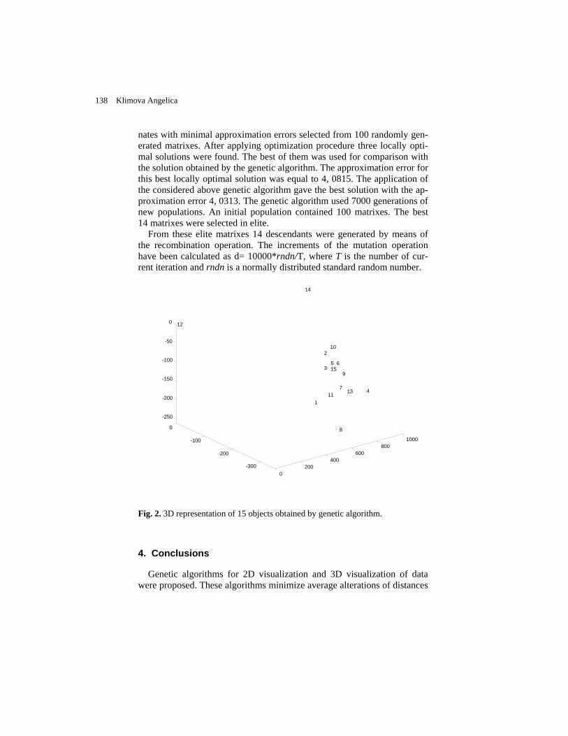
nates with minimal approximation errors selected from 100 randomly gen-erated matrixes. After applying optimization procedure three locally opti-mal solutions were found. The best of them was used for comparison with the solution obtained by the genetic algorithm. The approximation error for this best locally optimal solution was equal to 4, 0815. The application of the considered above genetic algorithm gave the best solution with the ap-proximation error 4, 0313. The genetic algorithm used 7000 generations of new populations. An initial population contained 100 matrixes. The best 14 matrixes were selected in elite.

From these elite matrixes 14 descendants were generated by means of the recombination operation. The increments of the mutation operation have been calculated as d= 10000*rndn/T, where T is the number of cur-rent iteration and rndn is a normally distributed standard random number.

0200

400600

8001000

-300

-200

-100

0 -250

-200

-150

-100

-50

0

8

111

713

39

15

4

5 6

210

14

12

Fig. 2. 3D representation of 15 objects obtained by genetic algorithm.

4. Conclusions

Genetic algorithms for 2D visualization and 3D visualization of data were proposed. These algorithms minimize average alterations of distances


initially given in n-dimensional attribute space. Application of this algo-rithm gives possibility to obtain usually the better results than by standard optimization procedure. A visualization of multivariate data as usually re-sults in distance alteration. For this reason additional methods of data analysis such as cluster analysis may be used independently from data visualization. Application of these methods to the same data gives possibil-ity to supplement the classification of data with visualization of data [6]. In the work [4] it was proposed the method of multistage visualization of data based on hierarchical clustering of data. In this approach the results of cluster analysis are supplemented by visual information about distances between objects and mutual location of clusters. On the other hand a repre-sentation of clusters of similar objects in 2D space gives possibility to “compensate” the distance alterations in 2D representation of data. The method of 3D visualization of data proposed here gives possibility to ex-tend on 3D case the method of hierarchical 2D visualization of data devel-oped in [4]. It is also supposed in the future work to extend the evolution-ary method of 3D visualization considered here on non-metric data visualization preserving the ordering of distances between objects [3].

Acknowledgment

The work is supported by RFFI grant 03-01-96245.

References

[1] R. Duda and P. Hart. Patten Classification and Scene Analysis, New York: Jon Wiley and Sons, 1973.

[2] E. Goldberg. Genetic algorithm in search Optimization and ma-chine learning, Addison-Wesley, MA, 1989.

[3] A. Ju. Terekhina. Data analysis by multidimensional scaling methods, Moscow: Nauka, 1986 (in Russian).

[4] Batyrshin I., Klimova A., Sheremetov L. On two dimensional visualization of hierarchical clustering. In: IEEE Int. Conf. Comp. Cybern, ICCC 2003, Siofok, Hungary, 2003, 181–184.

[5] V. Vasiliev, B. Iliasov. Intellectual systems of control with the use the genetic algorithms, Ufa, 1999 (in Russian).

[6] J. B. Kruskal. The relationship between multidimensional scal-ing and clustering, in: Classification and clustering (Ed. John Van Ryzin) New York: Acad. Press, 1977, 17-44 (in Russian).

[7] World Stock Market Data Base: www.countrybriefings.com


FUZZY GAMES, DECISIONS AND EXPERT SYSTEMS

Plenary Report

Vague Utilities in Cooperative Market Mareš Milan

Fuzzy Games and Decision Making

The Shapley Value for Games on Lattices (L-Fuzzy Games)

Grabisch Michel Optimal Strategies of Some Symmetric Matrix Games

De Schuymery Bart, De Meyer Hans and De Baets Bernard On strict Monotonic t-norms and t-conorms on Ordinal Scales

Batyrshin I.Z. and Batyrshin I.I. Belief Functions and the Imprecise Dirichlet Model

Utkin Lev V. Fuzzy Decision Making Using the Imprecise Dirichlet Model

Utkin Lev V. and Augustin Thomas

Fuzzy Expert Systems

A Fuzzy Expert System for Predicting the Effect of Socio-Economic Status on Noise-Induced Annoyance Zaheeruddin and Jain V. K.

The Knowledge Representation Model in Fuzzy Expert Systems Provided by Computing with Words and PRUF Language

Glova V.I., Anikin I.V., Katasev A.S. and Pheoktistov O.N

Decision Trees and Optimization

Construction of Incremental Fuzzy Decision Tree Borisov Arkady and Bikesheva Gulnara

Fuzzy Binary Tree Model for European-Style Vanilla Options Muzzioli Silvia and Reynaerts Huguette

Tree-Structured Smooth Transition Regression Correa da Rosa Joel, Veiga Alvaro, Medeiros Marcelo

Discrete Dynamic Programming With Outcomes In Fuzzy Ordered Structures Trzaskalik Tadeusz and Sitarz Sebastian

Vague Utilities in Cooperative Market

Milan MAREŠ Institute of Information Theory and Automation Academy of Sciences of the Czech Republic P.O.Box 18, 182 08 Praha 8, Czech Republic e-mail: [email protected]

Abstract: The Walras model of free exchange market and its relation to

the cooperative games theory is well known from the literature. Here, we formulate its modification in which some of its components, namely the utilities and prices, are vague, represented by fuzzy quantities. This vagueness appears natural if we consider the subjective character of utilities, and the variability of prices in free market. We discuss the relation of the presented model to the classical deterministic one. Some of its elementary properties are derived, too.

1 Introduction

There exist several economic equilibrium models focused on particular phenomena. One of them is the free exchange market model including no production or consumption and analyzing the exchange of goods among agents aiming to satisfy their individual demands under natural market constraints. These constraints follow from the existence of limited amounts of particular goods in the market, and from the necessity to respect some price relations. The optimal satisfaction of such agents’ needs is connected with the term of Walras equilibrium which is dealt in numerous works.

Here, we are interested in those which point at the close relation between such market model and some kind of coalitional games. It is presented, e.g., in [13], [11] and [12], and thoroughly analyzed in [4] where its asymptotic properties are considered, too. Papers [5], [6] and [7] have contributed to this model by including the possibility to form „strongly motivated“ coalitions of player whose members have a possibility to proceed cooperatively, to enter into the market with common property and to distribute the achieved wealth due to the needs of their participants without the limitations given by the existence of prices.

Both, the well known basic model as well as its modification mentioned above, are based on the assumption that all their elements are

exactly known. Nevertheless, in most of real markets this is not the truth. At least the subjective utilities of the goods may depend on the vagueness of human preferences, and also the prices vary in some interval with different degrees of possibility.

In the formulation of the fuzzy cooperative market model, we can be inspired by the concepts developed in the fuzzy cooperative games theory. Let us limit our attention on the fuzzification of the cooperative games with transferable utility (even if the fuzzy cooperation in games with non-transferable utility is studied in the literature, as well). First, the models of fuzzy cooperative games can be based either on the fuzzification of the coalitions (see, e.g., [1], [2], [3]) or on the fuzzification of the expected pay-offs (see, e.g., [9], [10]) with wide application of fuzzy quantities theory [8]. The vagueness of utilities and prices implies rather the vagueness of the expected pay-offs (or profits) and, consequently, we focus our attention of the model of markets where individual utilities are fuzzy functions (i.e., function with values in fuzzy quantities) and prices are fuzzy quantities. The game theoretical counterparts of such markets are the games described in [9].

In the following section we briefly recall the deterministic model of free exchange market, introduce the notations and concepts for the handling fuzzy quantities, formulate the fuzzified alternative of the market and its equilibrium, and show some results describing its basic properties.

2 Preliminary Concepts

In this section, we briefly recollect some notions important for the formulation of the suggested model. Namely, we introduce the original deterministic free exchange market, and the elements of the fuzzy quantities theory.

In the whole paper, we denote by I the (non-empty and finite) set of agents; to simplify the notations, we put I = 1, 2, ..., n. Every set of agents K ⊂ I is called a coalition. By R we denote the set of real numbers,

+R is the set of non-negative real numbers, and kR , kR+ are set of k-dimensional vectors for positive integer k.

2.1Coalitional Game If v is a mapping connecting each coalition K with a real number

v(K), such that v(∅)=0 then the pair (I,v) is a coalitional game. We say that (I,v) is superadditive iff for any pair of disjoint coalitions K,L

144 MareŠ Milan

).()()( LvKvLKv +≥∪ Every real-valued vector Iiix ∈= )(x is called an imputation. A set of

imputations )(,),(:)( KvxIvxxC

Ki iIKiIiIii ≥∀≤∑== ∑∈⊂∈∈x is called a core of the game in question. If I2⊂M is a class of

coalitions such that for every Ii∈ there exists M∈K such that Ki∈ , then the set

)(: IvxRC iIin ≤∑∈= ∈xM and for any )(, KvxK iKi ≥∑∈ ∈ M .

2.2 Cooperative Market Let us consider n agents who share m types of goods. The symbol

mjIixij ,...,1,, =∈ denotes the amount of the j-th good owned by agent i.

We suppose that 0≥ijx for all i, j, denote Ii

ix ∈= )(X ,

Iixx mjij

i ∈= = ,)( ,...,1 . The structure X of vectors ni Rx ∈ is called an allocation of goods. There exists exactly one allocation of goods, we denote it Ii

ia ∈= )( , mi Ra +∈ , representing the initial allocation. By the

cartesian product i

IiX

∈= XX , where

: mii RxX +∈= mj ,...,1=∀ , Iiax i

jIiIiij ∈∑≤ ∈∈∑ , , we denote the set

of all theoretically possible allocations. Let us suppose, further, that each agent Ii∈ evaluates the realized

allocation by means of his individual preferences represented by utility function Rui →X: . The quadruple

))(,)(,,( Iii

Iii auI ∈∈= Xm whose components are specified above, is called a market. Finally, the goods are connected with some prices. The price vector

is denoted mjjpp ,...1)( == , where 0>jp for all j=1,...,m, and P is the set of all admissible price vectors. We suppose that Pp∈ are row-vectors, meanwhile ii Xx ∈ are columns, so that the scalar products ixp. have sense. Each pair ( x ,p) formed by allocation and prices Pp∈∈ ,Xx , is called state of market. For every agent Ii∈ we define the set

iiip apxp ..: ≤∈= XxB ,

called his budget set.

Vague Utilities in Cooperative Market 145

A state of market ),( px is called the (Walras) equilibrium iff ipx B∈ for all Ii∈ ,

if ipy B∈ then ).()( yuxu ii ≥

The above equilibrium concept can be extended into a cooperative one. It is done, e.g., in [11] or [12]. Here, we recollect its modification [5], [6]. Let us consider a non-empty coalition IK ⊂ , and denote for a price-vector p and allocation Xx∈ the set

..: ∑∑ ∈∈≤∈=

Kii

KiiK

p apypXxB ,

which we call the budget set of coalition K and the function RuK →X: such that

.),()( Xxxx ∈= ∑∈Ki iK uu

If I2⊂M is a set of coalitions such that for each Ki∈ , there exists a coalition M∈K such that Ki∈ , then we say that a state of market ),( px is an M -equilibrium iff

KpB∈x for all M∈K ,

∑∑∈∈

=∈=Ki

ij

Ki

ijKK axuu ,:)(max)( Xxxx for all mj ,...,1= .

The cooperative definition of the market introduced above, suggested in [5] and [6], and modified in [7], follows from the latent assumption that there exist groups of agents being strongly motivated for cooperation reaching beyond the standard market principles (e.g., families, politicaly or nationaly motivated allies, etc.). Their members aim to maximize their individual profit. But they are able to do so via maximizing the common profit of the coalition and dividing it among its members due to some „just“ rules of the cooperative game theory.

If IK ⊂ then we define a value RKv ∈)( such that ..,1 allfor ,:)(max)( ∑ ∑

∈ ∈

==∈=Ki Ki

ij

ijKm m,.jaxuKv Xxx .

The pair ),( mvI , where Rv I →2: and 0)( =∅v , is said the market game of the market m . The relation between the market equilibria and the core of the market game is treated by the main results of the referred market theory.

2.3 Fuzzy Quantity

The main fuzzy set theoretical tool used below is the concept of fuzzy quantity [8]. We use this term for any fuzzy subset a of the real line, with

membership function [ ]1,0: →Raµ . We suppose that 1)( =xaµ for

146 MareŠ Milan

some Rx∈ , and the support set of aµ is limited. The fuzzy quantities can be algebraically processed by means of so called extension principle. Here,

we need the operations of addition and product with crisp number. If a,b are fuzzy quantities with ba µµ , , and Rr ∈ is crisp real number, then

ba⊕ and r.a are fuzzy quantities, too, and [ ]))(),(min(sup)( yxxx ba

Ryba −=

∈⊕ µµµ

)/()(. rxx aar µµ = if 0≠r , 0)(,1)0( .0.0 == xaa µµ if 0≠x . There exist various definitions of the ordering relation between fuzzy

quantities. Here, we use the one due to which such ordering ≥ is a fuzzy relation, too. It is defined by membership function (.,.)ν connecting each ordered pair of fuzzy quantities a, b with a real number

[ ]yxRyxyxba ba ≥∈= ,,:))(),(min(sup),( µµν . The value ),( baµ evaluates the possibility of ba ≥ in the fuzzy

ordering ≥ .

3 Fuzzy Market

The original market model ))(,)(,,( Iii

Iii auI ∈∈= Xm and its equilibrium are constructed as deterministic concepts. In the everyday reality, there is lot of vagueness hidden in the market situation. We focus our attention on the cases in which the numerical evaluations of allocations, i.e., the utility functions and prices, are subjective or destabilized.

In the next sections, we suppose that for each allocation Xx∈ and each agent Ii∈ , the utility value is a fuzzy quantity, let us denote it

( )xFiu . If )(xiu is the deterministic utility value in the above market m ,

if ]1,0[:(.), →Ri xµ is the membership function of x)(Fiu , and if

1))((, =xx ii uµ for all Xx∈∈ ,Ii , then we say that Fiu is a fuzzy

extension of the utility function ui. Similarly, we suppose that the prices pj, j=1,...,m are vague. Each

of them is represented by fuzzy quantity Fjp with membership function

]1,0[: →Rjπ such that 0for 0)( ≤= ξξπ j , and, moreover, the vector

mjj ,...,1 )( =π of membership functions is such that

.),...,,( if 0)().....().( 212211 Pmmm ∉= ξξξξπξπξπ If Pp∈ is a crisp


price vector used in the above market m, if ,,...,1 ,1)( mjp jj ==π then

we say that mjpp Fj

F ,...,1)( == is fuzzy extension of prices p.

The quadruple ))(,)(,,(FIi

iIi

Fi auI ∈∈= Xm , is called fuzzy

market. If the fuzzy utilities Fiu are fuzzy extensions of Iiui ∈, , then mF

is called fuzzy extension of the market m. Remark 1. If mRP += then for every vector of fuzzy prices

mjFj

F pp ,...,1)( == there exists Pp∈ such that pF is fuzzy extension of p. Remark 2. If 1...: 21 =+++∈= + m

m pppRpP and if the vector pF is such that

0... if 0)()...( 111 ≠++= mmm ξξξπξπ then there exists Pp∈ such that pF is fuzzy extension of p. Let us consider a non-empty coalition K. Let Ru F

K →X: be a

fuzzy function such that for any )(x , Xx FKu∈ is a sum of

Kiu Fi ∈),(x , in the sense of Subsection 2.3. Then )(xF

Ku is a fuzzy quantity with membership function ].1,0[:, →RK xµ

Remark 3. If 0, ≠⊂ KIK , and if for all F

iuKi ,∈ is fuzzy extension of ui then

( ) ,1)(, =∑ ∈ xx iKiK uµ as follows from the properties of addition of fuzzy quantities (see [8]). The vagueness of the utilities and prices brings its consequences in

the vagueness of other components derived from them. It regards, especially, the budget sets and equilibria.

In the fuzzy market mF the product p.xi, xi∈Xi, p∈P, means a product of crisp vector xi and vector of fuzzy quantities pj, j=1,...,m, i.e.

,...... 11imm

ii xpxpxp ⊕⊕= where each component of the sum is a product of fuzzy quantity pj and

crisp number ijx and the entire sum is a sum of fuzzy quantities. This is

true even in the case of initial allocations Iiai ∈, . It means that the budget sets in the fuzzy market are based on the ordering relation over fuzzy quantities. We have accepted, in Subsection 2.3, the principle that

148 MareŠ Milan

such relation is fuzzy, as well. Its membership function was denoted by ν. Hence, we define the fuzzy budget set i

pF

FB for Ii∈ and fuzzy prices pF

as fuzzy subset of X with membership function ]1,0[:, →Xpiβ , where

.)( , ).,.()(, Ii

iiFiFpi

xxpapF ∈== xx νβ

Lemma 1. If the fuzzy market mF is fuzzy extension of market m, if pF

is fuzzy extension of prices p, and if ipB is a budget set of m for Ii∈ ,

then 1)(, =xFpiβ for all ipB∈x .

Proof. The statement follows from the previous definitions. If pF is fuzzy

extension of market m , if pF is fuzzy extension of p then 1)( =jj pπ for

all j=1,2,...,m. Let us denote by µx the membership function of the fuzzy quantity i

mFm

iF xpxp ⊕⊕ .... 11 . Then .1).( =ixpxµ Similarly, let aµ

denote the membership function of im

Fm

iF apap ..... 11 ⊕⊕ for the initial

allocation a and Ii∈ . Then 1).( =ia apµ . Due to the definition of the

membership ν, if ipB∈x then ii papx ≤ for all Ii∈ , and, consequently,

.1)( =xν Having introduced the fuzzy budget sets, we may formulate the

concept of the state of fuzzy market mF as a pair (x, pF), where X∈x and pF is the vector of fuzzy prices, such that x belongs to the fuzzy budget set and its fuzzy utility is maximal. This heuristic formulation has to be specified. The property of being equilibrium of a fuzzy market is a fuzzy property and the equilibria form a fuzzy subset of the class of all states of the fuzzy market. Let us denote the membership function of this fuzzy set by ρ, and for any state ),( Fpx formed by (crisp) allocation and fuzzy prices the value ),( Fpxρ denotes the possibility that (x,pF) may be an equilibrium of mF. By means of generalization of the deterministic equilibrium concept and using the above definitions we may define the values of ρ by the following procedure:

- Denote )(xipFβ the possibility that x belongs to the fuzzy budget

set, Ii∈ . - Denote [ ]Xyyxy ∈= ∈ :)(),((),(min)( Xyx F

iFi

ipi uuF νβγ , for all

Ii∈ , the possibility that the fuzzy utility of allocation x for agent i


is greater than the utility of any other allocation possibility belonging to the same fuzzy budget set.

- Then we put ).:)(),(min(),( Iip i

ip

FF ∈= xxx γβρ

The equilibrium of fuzzy market mF reflects the basic structures of its fuzzy components. Namely, it extends the equilibrium of the deterministic market.

Theorem 1. Let mF be fuzzy extension of market m, and let pF be fuzzy

extension of prices Pp∈ . Let the state of market )( p,x be an

equilibrium of m. Then .1),( =Fpxρ

Proof. Using Lemma 1, we know that for all Ii∈ , .1)( =xipFβ The

equilibrium assuption about ),( px immediately implies that 1))(),(( =yx F

iFi uuν for all Xy∈ such that 1)( =yi

pFβ , where the

definition of Fiu was used. These equations imply the statement.

The theorem means that the equilibrium of fuzzy market is a fuzzy

extension of the deterministic equilibrium of the original deterministic market.

4. Cooperative Fuzzy Market

The above procedure can be repeated also for the concept of M-

equilibrium. Let m be a market,let mF be its fuzzy extension, let pF be vector of fuzzy prices which is a fuzzy extension of Pp∈ . Let, finally,

I2⊂M fulfil assumptions of Subsection 2.2. If IK ⊂ is a non-empty coalition then we introduce the fuzzy

subset X of KpFB with membership function K

pFβ , where

,)( ),.,.()( Xxx ∈== ∈IiiKFKFK

pxxpapF νβ where ν represents the

fuzzy ordering relation, and for any x∈X the symbols KF xp . and KF ap . denote the sums of fuzzy quantities iF xp . , or iF ap . , summed over all

150 MareŠ Milan

Ki∈ , respectively. The above fuzzy set is called fuzzy budget set of coalition K.

Analogously to the previous section, we define the M-equilibrium of mF as a fuzzy subset of the class of all states ),( Fpx described by a membership function Mρ , where

):)(),(min(),( MKp KKp

FF ∈= xxxM γβρ

where KpFβ is defined above, and

).:))(),((),(min()( Xyyxyx ∈= FK

FK

KpK uuF νβγ

Then the following statement can be derived analogously to the proof of the previous Theorem 1.

Theorem 2. Let mF be fuzzy extension of market m, and let pF be fuzzy

extension of prices Pp∈ . Let the state ),( px be an M-equilibrium of m for some class of coalitions. Then

.1),( =FM pxρ

The following two statements immediately follow from definitions. Remark 4. If ,...,2,1 n=M is the class of all one-agent

coalitions then the M-equilibrium is identical with the equilibrium for any fuzzy market mF.

Lemma 2. If M=I is the one-coalition class then for any fuzzy market

mF and any fuzzy price vector pF there exists an M-equilibrium ),( Fpx .

Proof. For this specific case of M the budget set i

jIiijIi

Ip axmjB ∈∈ ∑=∑=∀∈= ,,...,1:Xx is independent on the

price vector p. The existence of the maximal value of fuzzy coalitional utility function )(xF

Ku for all pB∈x follows from the definition of Fiu and F

Ku , and from the properties of fuzzy ordering.

5. Conclusive Remarks


The above brief formulation of the fuzzy market and cooperative fuzzy market model covers only one of possible approaches to the fuzziness in market. Let us mention at least two alternatives. Both of them are inspired with fuzzy cooperative games theory.

The fuzziness of the market activities may regard not only utilities and prices (i.e., the quantitative values treated by the market model) but also the participation of agents in coalitions. It is possible (and realistic) to admit that each player may participate in more coalitions with different degree of participation (compare with [1], [2], [3]). This alternative approach opens qualitatively new aspects of the market model. The concept of M-equilibrium (where the coalitions in M need not be disjoint) offers a frame for the formal representation of such market.

On the other hand, the fuzziness of the quantitative aspects of market need not be represented by the fuzzification of its particular components like utilities and prices, but by analyzing a fuzzy subclass of the class of all deterministic markets with the set of agents I and initial allocation X a ∈= ∈Ii

ia )( . The difference of both approaches is analogous to the difference between the fuzzy cooperative game models given in [9] and [10]. Both of these models are mutually related – the memberships of fuzzy class of crisp markets can be derived from the memberships of fuzzy utilities.

The analysis of both these alternatives may be done in some following research.

References

[1] J. P. Aubin: Cooperative fuzzy games. Math. Oper. Res. 6 (1981), 1-

13. [2]

D. Butnariu: Fuzzy games: a description of the concept. Fuzzy Sets

and Systems 1 (1978), 181-192. [3] D. Butnariu, E. P. Klement: Triangular Norm – Based Measures and

Games With Fuzzy Coalitions. Kluwer, Dordrecht 1993. [4] W. Hildenbrand: Core and Equilibria of a Large Economy. Princeton

Univ. Press, Princeton 1974. [5] M. Mareš: Suggestion of a cooperative market model. Kybernetika

12 (1976), 6, 439-450. [6] M. Mareš: On cooperative games connected with markets.

Kybernetika 12 (1976), 6, 451-461. [7] M. Mareš: General coalition games and markets. Transactions of

„Operations Research Tagung. Oberwolfach 1978“, Springer-

152 MareŠ Milan

Verlag, Berlin 1979, 217-222. [8] M. Mareš: Computation Over Fuzzy Quantities. CRC-Press, Boca

Raton 1994. [9] M. Mareš: Fuzzy Cooperative Games. Physica-Verlag, Heidelberg

2001. [10]

M. Mareš, M. Vlach: Fuzzy classes of cooperative games with transferable utility. Mathematica Japonica. To appear in 2004.

[11]

J. Rosenmüller: Kooperative Spiele und Märkte. Springer-Verlag, Heidelberg 1971.

[12]

J. Rosenmüller: The Theory of Games and Markets. North Holland, Amsterdam 1982.

[13]

L. S. Shapley, M. Shubik: On market games. Journal of Econ. Theory. Vol. I (June 1969), No.1


The Shapley value for games on lattices(L-fuzzy games)

Michel GRABISCHUniversite Paris I - Pantheon-Sorbonne ; LIP68, rue du Capitaine Scott 75015 Paris, Franceemail [email protected]

Abstract

Several concepts of cooperative games (non monotonic fuzzy measures) havebeen proposed in the past, which can be all considered as games on lattices. Forthe case of distributive product lattices, we propose a general formulation of theShapley value, together with an axiomatization. These games could be called L-fuzzy games. The case of global games proposed by Gilboa and Lehrer, where theunderlying lattice is the partition lattice, is also cited.

1 Introduction

The field of cooperative game theory [1, 13] has been enriched these recent years bymany new kinds of game, trying to model in a more accurate way the behaviour ofplayers in a real situation. To the original notion of cooperative game (otherwise said,non-monotonic fuzzy measures), where to each coalition of players taking part into thegame, an asset is associated, many variations have been added, let us cite for examplebi-cooperative games proposed by Bilbao et al. [1] (see also Labreuche and Grabisch[12] for a slightly different view) where players are either defenders, defeaters or donot participate, ternary voting games of Felsenthal and Machover [5], where voterscan choose between voting in favor or against, or abstain, multichoice games of Hsiaoand Raghavan [11] where each player has several possible levels of participation to thegame, games with r alternatives proposed by Bolger [3], fuzzy games [4] where eachplayer has a degree of participation, global games of Gilboa and Lehrer [6], k-stagegames, games defined on pairs (S, P ), where S is a set and P a partition containing it,etc.

Let us denote N = 1, . . . , n the finite set of players. As remarked by Gilboaand Lehrer [6], many of the above examples can be considered as particular cases ofgames on lattices, i.e. functions v : (L,≤) −→ R where (L,≤) is a lattice, and suchthat v(⊥) = 0, ⊥ denoting the bottom element of L. This point of view has also beenadvocated by Grabisch and Labreuche, in a larger perspective of decision theory anddata analysis [9, 10]. For example, classical cooperative games correspond to the casewhere (L,≤) is the lattice (2N ,⊆) of all coalitions of players ordered by inclusion,

bi-cooperative games and ternary voting games correspond to the case where L = 3N ,multichoice games correspond to L = (m+1)N , with m the number of different levelsof participation, fuzzy games to L = [0, 1]N , and global games are built on the latticeof partitions of N . We remark that most of the examples of lattices are products of nlattices, all identical. This is rather natural since each dimension correspond to a player,and this was the motivation of Grabisch and Labreuche for considering only productlattices L = L1 × · · · × Ln. Then interpreting the elements of Li as level or degree ofparticipation of player i to the game, such games could be called L-fuzzy games, in thesame sense that Goguen [7] proposed L-fuzzy sets, i.e. valued on some lattice insteadof [0, 1]. However in the sequel, we will keep the term “games on (product) lattices”,since this is more precise.

A central question in game theory is how to compute a value or solution concept fora game, i.e. how to individually reward players when the game has been played. Forclassical game, this is done by the well-known Shapley value [14]. For all the abovecited examples, authors have tried to generalize or adapt the original Shapley valueto their own framework. In this paper, we propose a general formulation for the caseof product lattices, together with an axiomatization in the spirit of Weber [15]. Thecase of global games, which cannot be included into our framework, will be separatelyexplained.

Similar work has been done by Bilbao [1] for games defined on other general struc-tures (convex geometries and matroids).

To avoid heavy notations, we will often omit braces for singletons, and cardinalityof sets S, T will be denoted by s, t. etc.

2 Classical cooperative games

Let N := 1, . . . , n be the finite set of players. A game on N is any function v :2N −→ R, such that v(∅) = 0. We call coalition any subset of N . For any coalitionA ⊆ N , v(A) is the asset or income the coalition A will win if the game is played, i.e.if all players equally participate to the game, players in Ac playing against A (or do notparticipate). We denote G(2N ) the set of all games on N .

Player i is said to be dummy for v if v(S ∪ i) = v(S) + v(i), for all coalition S.Player i is null for v if v(S ∪ i) = v(S). Observe that a null player is dummy, and adummy player with v(i) = 0 is null.

A value or solution concept is any function φ : G(2N ) −→ RN , which represent an

assignment of income to each player. Let us present examples of properties or axiomsφ may fulfil.

• linearity (l): φ is linear over G(2N ).

• dummy axiom (d): if i is dummy for v, then φi(v) = v(i).

• null axiom (n): if i is null for v, then φi(v) = 0.

• symmetry (s): φ does not depend on the labelling of the players.

• efficiency (e):∑

i∈N φi(v) = v(N).

The Shapley value for games on lattices (L-fuzzygames) 155

Note that the dummy axiom is stronger than the null axiom. The Shapley value [14] isthe unique value satisfying axioms l, n, s and e, and is given by

φi(v) :=∑

S⊆N\i

(n − s − 1)!s!

n![v(S ∪ i) − v(S)]. (1)

Weber [15] has shown how precisely each axiom contributes to the result. Since we willfollow the same approach, we briefly present his results. Linearity implies the existenceof 2n real constants ai

S such that φi(v) =∑

S⊆N aiSv(S). If the null axiom is added,

then these constants are pairwise opposite so that φi(v) =∑

S⊆N\i piS [v(S ∪ i) −

v(S)], with piS := ai

S∪i. If the dummy axiom replaces the null axiom, then in additionthe 2n−1 coefficients pi

S satisfy∑

S⊆N\i piS = 1. If the symmetry axiom is added,

then coefficients piS depend only on the cardinality of S, so that only n coefficients

p0, . . . , pn−1 are needed (n − 1 if the dummy axiom replaces the null axiom). Lastly,if efficiency is added, the unique possibility are the coefficients of the Shapley value in(1).

3 Games on product lattices

As remarked in the introduction, most of more general concepts of games can be em-bedded into a general notion of game on lattices, where the lattice is a product latticeL := L1 × · · · ×Ln. A general framework for these games has been proposed by Gra-bisch and Labreuche, aiming at defining interaction (a generalization of the Shapleyvalue to coalitions). Since our aim is to focus on the Shapley value, we restrict here tonecessary notions and avoid intricacies (see [9, 10] for details).

3.1 Preliminaries

We recall elementary definitions for lattices (see e.g. [2]), in a finite setting. A latticeis a set L endowed with a partial order ≤ such that for any x, y ∈ L their least upperbound x∨y and greatest lower bound x∧y always exist. For finite lattices, the greatestelement of L (denoted >) and least element ⊥ always exist. x covers y (denotedx y) if x > y and there is no z such that x > z > y. The lattice is distributive if∨,∧ obey distributivity. An element j ∈ L is join-irreducible if it cannot be expressedas a supremum of other elements. Equivalently j is join-irreducible if it covers onlyone element. Join-irreducible elements covering ⊥ are called atoms, and the latticeis atomistic if all join-irreducible elements are atoms. The set of all join-irreducibleelements of L is denoted J (L).

An important property is that in a distributive lattice, any element x can be writtenas an irredundant supremum of join-irreducible elements in a unique way (this is calledthe minimal decomposition of x).

In a finite setting, Boolean lattices are of the type 2N for some set N , i.e. they areisomorphic to the lattice of subsets of some set, ordered by inclusion. Boolean latticesare atomistic, and atoms corresponds to singletons. A linear lattice is such that ≤ is atotal order. All elements are join-irreducible, except ⊥.

156 Grabisch Michel

Given lattices (L1,≤1), . . . , (Ln,≤n), the product lattice L = L1 × · · · × Ln isendowed with the product order ≤ of ≤1, . . . ,≤n in the usual sense. Elements of x canbe written in their vector form (x1, . . . , xn). We use the notation (xA, y−A) to indi-cate a vector z such that zi = xi if i ∈ A, and zi = yi otherwise. Similarly L−i denotes∏

j 6=i Lj . All join-irreducible elements of L are of the form(⊥1, . . . ,⊥j−1, i0,⊥j+1, . . . ,⊥n), for some j and some join-irreducible element i0of Lj . A vertex of L is any element whose components are either top or bottom. Wedenote Γ(L) the set of vertices of L. Note that Γ(L) = L iff L is Boolean.

Let (L,≤) be some finite lattice, and consider f : L −→ R, and a join-irreducibleelement i of L. The derivative of f w.r.t i at point x is defined as [8]: ∆if(x) :=f(x ∨ i) − f(x). This definition can be considered as a first-order derivative. Onecan iterate the definition, taking several join-irreducible elements. If the lattice is dis-tributive, since any element y can be decomposed in a minimal and unique way onjoin-irreducible elements, the derivative w.r.t. y, ∀y ∈ L, can be defined as well. Thederivative is said to be Boolean if x∨ i x (or more generally if [x, x∨y] is a Booleanlattice).

3.2 The framework

We consider distributive finite lattices L1, . . . , Ln and their product L := L1×· · ·×Ln.A game on L is any function v : L −→ R such that v(⊥) = 0. The set of such gamesis denoted G(L).

This can be interpreted as follows, in the setting of game theory (for other interpre-tations, see [9, 10]). Lattice Li represents the (partially) ordered set of actions, choices,levels of participation of player i to the game. Each lattice may be different.

Let us give examples of this general framework. Let us consider that all latticesLi’s are identical, so that the product lattice is of the form Ln. The simplest exampleis to take for L the smallest lattice L := ⊥,>, also denoted 2 since it has only 2elements. Note that this is a linear lattice. Then we get 2n, i.e. we recover classicalgames, defined on the power set of N ordered by inclusion, which is a Boolean lattice.Here > has the meaning of participating to the game, and ⊥ means no participation (orplaying against).

Bi-cooperative games and ternary voting games correspond to the case L1 = · · · =Ln = 3, i.e. there are three possible actions, totally ordered 1.

Multichoice games correspond to all cases where L1 = · · · = Ln = m + 1, i.e. alinear lattice of m actions, plus the ⊥ action which correspond to do nothing.

Fuzzy games correspond to the case L1 = · · · = Ln = [0, 1]. Considering fuzzysets valued on some lattice (the so-called L-fuzzy sets of Goguen [7]), it is clear thatour proposal of games on product lattice may be called also L-fuzzy games.

Global games do not fit in our picture since the underlying lattice is the partitionlattice, which is not a product lattice. We will consider this case later on.

1This is true up to the fact that for bi-cooperative games as defined in [1, 12], the condition v(⊥) = 0is replaced by v(0, 0, . . . , 0) = 0, if we denote all Li by ⊥, 0,>. To fit with this definition, a slightlydifferent framework has to be defined, which we do not address in this paper.


3.3 Value for games on lattices

In [9, 10] a general form for a solution concept was proposed for games on productlattices. We give its definition. We use the notation L−j :=

∏i6=j Li.

Definition 1 Let i = (⊥1, . . . ,⊥j−1, i0,⊥j+1, . . . ,⊥n) be a join-irreducible elementof L. The value w.r.t. i of v is any function of the form

φi(v) :=∑

x∈Γ(L−j)×i0

α1h(x)∆iv(x), (2)

where i0 is the (unique) element covered by i0 in Lj , h(x) is the number of componentsof x equal to >l, l = 1, . . . , n, and α1

k ∈ R for any integer k.

Observe that the constants α1h(x) do not depend on i. Also, the derivative is Boolean.

Let us show that this definition encompasses the case of classical games, i.e. whereL is the Boolean lattice 2n. Join-irreducible elements of L are singletons, as remarkedbefore all elements in L are vertices, and h(x) is the cardinality of sets. Also for S ⊆N \ i, ∆iv(S) = v(S ∪ i)− v(S), thus we get φi(v) =

∑S⊆N\i α1

|S|[v(A∪ i)− v(S)]for any i ∈ N , as desired (see Section 2).

In [9, 10], Grabisch and Labreuche showed that if a condition similar to efficiencywas added, specifically

∑i∈J (L) I(i) = v(>) − v(⊥), then the coefficients were de-

termined, and equal to the Shapley coefficients α1k = (n−1−k)!k!

n! .Let us show that under suitable axioms, one can recover this result in a unique way.

3.4 Axiomatization of the Shapley value for games on product lat-tices

We consider the linear case, where L =∏n

i=1 Li, with Li a linear lattice denotedLi := 0, 1, 2, . . . , li. With some abuse of notation, for some k ∈ Li we write ki for(0−i, ki), i.e. (0, . . . , 0, k, 0 . . . , 0), where k is at the ith position.

Our aim is to define φki(v), for any i ∈ N , any k ∈ Li, k 6= 0 (i.e. ki ranges over

all join-irreducible elements of L).For some k ∈ Li, k 6= 0, player i is said to be k-dummy if v(x, ki) = v(x, (k −

1)i) + v(ki), for any x ∈ L−i.

Dummy axiom (D): ∀v ∈ G(L), for all join-irreducible ki, φki(v) =

v(ki) if i is k-dummy.

For some k ∈ Li, k 6= 0, player i is said to be k-null if v(x, ki) = v(x, (k − 1)i),for any x ∈ L−i.

Null axiom (N): ∀v ∈ G(L), for all join-irreducible ki, φki(v) = 0 if i is

k-null.

Remark that i is k-dummy and v(ki) = 0 implies i is k-null, and i is 1-null implies i is1-dummy.

158 Grabisch Michel

Linear axiom (L): φv is linear on the set of games, i.e. for any join-irreducible ki, φki

(v) =∑

x∈L akix v(x), with aki

x ∈ R.

Proposition 1 Under (L) and (N), ∀v ∈ G(L), for all join-irreducible ki, φki(v) =∑

x∈L−i

pkix ∆ki

v(x, (k − 1)i), with pkix ∈ R.

Recall that ∆kiv(x, (k − 1)i) = v(x, ki) − v(x, (k − 1)i).

Let us see what we get if add the dummy axiom.

Proposition 2 Under (L), (D) and (N), ∀v ∈ G(L), for all join-irreducible ki, φki(v) =∑

x∈L−i

pkix ∆ki

v(x, (k − 1)i), with pkix ∈ R, and

∑x∈L

−ipki

x = 1.

Let σ be a permutation on N . With some abuse of notation we write σ(x) :=(xσ(1), . . . , xσ(n)).

Symmetry axiom (S): φσ(ki)(v σ−1) = φki(v), for any game v, any

join-irreducible ki.

Proposition 3 Under (L), (N) and (S), φki(v) =

∑x∈L

−ipk

n1,...,nl∆ki

v(x, (k − 1)i),where l := max(l1, . . . , ln), and nj is the number of components of x being equal toj.

Difference axiom (Di) Let us consider v1, v2 on L such that for somei ∈ N and some k ≥ 2, v2(x, ki) − v2(x, (k − 1)i) = v1(x, (k −1)i) − v1(x, (k − 2)i), ∀x ∈ L−i. Then for any such games φki

(v2) =φ(k−1)i

(v1).

The axiom says that when a game (v2) is merely a shift of another game (v1) concerningplayer i and level k, the Shapley values are the same. This implies that the way ofcomputing φv does not depend on the level k, as shown in the next proposition.

Proposition 4 Under axioms (L), (N) and (Di), pkix = p

(k−1)ix , for all x ∈ L−i, ∀i ∈

N , ∀k ∈ Li, k 6= 0.

Recall that J (L) is the set of all join-irreducible elements of L.

Efficiency axiom (E):∑

ki∈J (L) φki(v) = v(>) − v(⊥).

Proposition 5 Suppose L1 = L2 = · · ·Ln =: L. Under axioms (L), (N), (S) and (E),the coefficients pk

n1,...,nlsatisfy pl

0,...,0,n−1 = 1/n, p10,...,0 = 1/n, and nlp

ln1,...,nl−1 +∑l−1

j=1 nj(pjn1,...,nj−1,...,nl

− pj+1n1,...,nj−1,...,nl

) = (n − n1 − · · · − nl)p1n1,...,nl

.

The final result is the following.

Theorem 1 Suppose L1 = L2 = · · ·Ln =: L. Under axioms (L), (D), (S), (Di) and(E),

φki(v) =

∑x∈Γ(Ln−1)

(n − nl − 1)!nl!

n![v(x, ki) − v(x, (k − 1)i)],

where Γ(Ln−1) is the set of vertices of Ln−1.


It is remarkable that only vertices of L−i remain in the summation, which justifies thegeneral form given in (2).

Note that if axiom (D) is replaced by axiom (N), then coefficients pn1,...,nlwith

n1, n2, . . . , nl−1 6= 0 are not determined, and so the summation is not restricted tovertices of L−i.

4 Global games

We briefly describe global games as proposed by Gilboa and Lehrer [6]. In globalgames, all players tend to a global goal which will benefit to all of them if is attained(e.g. environment problems like water pollution, diminishing ozone layer, greenhouseeffect, etc.), and a game v modelizes the global utility for a given profile of cooperation,represented as a partition of all players. Denoting Π(N) the set of all partitions of N ,we have v : Π(N) −→ R.

A partition π is coarser than a partition π′ (denoted π w π′) if for every A ∈ πthere exists B ∈ π′ such that A ⊇ B. Then (Π(N),w) is a lattice, known as thepartition lattice, top being N and bottom being ii∈N

The partition lattice is an example of a geometric lattice (atomistic and upper semi-modular). It is not distributive. This lattice being not a product lattice, our frameworkdoes not apply. Gilboa and Lehrer have proposed axioms for defining the Shapleyvalue, which we present below.

To each global game h, we assign a (classical) cooperative game vh, called theinduced game, as follows: vh(A) := h(A, ii6∈A), ∀A ⊂ N, A 6= ∅. A playeri is null2 for global game h if for all partition π, h(π) = h(π ∧ N \ i, i). Twoplayers i, j are interchangeable for h if for all partition π, h((π ∧ N \ i, i) =h(π ∧ N \ j, j). Gilboa and Lehrer defined the following axioms for a value φon G(Π(N)):

Linearity (LGL): φ is linear on G(Π(N)).

Null axiom (NGL): for all h ∈ G(Π(N)), for all i ∈ N , if i is null for h,then φi(h) = 0.

Interchangeability (IGL): for all h ∈ G(Π(N)), for all interchangeablei, j, φi(h) = φj(h).

Efficiency (EGL):∑

i∈N φi(h) = h(N).

Note that these axioms are also close to the original ones of Shapley, interchangeabilityplaying the role of symmetry. They proved the following.

Theorem 2 The unique value (called the Shapley value) satisfying axioms (LGL),(NGL), (IGL), and (EGL) is equal to the Shapley value of the induced game: φi(h) =φi(vh).

2Gilboa and Lehrer called this axiom “dummy”, but it seems to correspond more to the null axiom.

160 Grabisch Michel

As remarked by Gilboa and Lehrer, it is remarkable that all partitions π ∈ Π(N) do notintervene in the Shapley value, but only the following ones A, ii6∈AA⊆N

are used. These partitions could be called vertices partitions, and we recover what wehave found in our framework, that only vertices of L−i are used. This fact suggests thata yet more general framework encompassing our approach and global games shouldexist.

References[1] J.M. Bilbao. Cooperative games on combinatorial structures. Kluwer Academic Publish-

ers, 2000.

[2] G. Birkhoff. Lattice Theory. American Mathematical Society, 3d edition, 1967.

[3] E.M. Bolger. A consistent value for games with n players and r alternatives. Int. J. ofGame Theory, 29:93–99, 2000.

[4] D. Butnariu and E.P. Klement. Triangular norm-based measures and games with fuzzycoalitions. Kluwer Academic Publishers, 1993.

[5] D. Felsenthal and M. Machover. Ternary voting games. Int. J. of Game Theory, 26:335–351, 1997.

[6] I. Gilboa and E. Lehrer. Global games. Int. J. of Game Theory, 20:129–147, 1991.

[7] J.A. Goguen. L-fuzzy sets. J. Math. Anal. Appl., 8:145–174, 1967.

[8] M. Grabisch and Ch. Labreuche. Capacities on lattices and k-ary capacities. In 3d Int, Conf.of the European Soc. for Fuzzy Logic and Technology (EUSFLAT 2003), pages 304–307,Zittau, Germany, September 2003.

[9] M. Grabisch and Ch. Labreuche. Interaction between attributes in a general setting forknowledge discovery. In 4th Int. JIM Conf. (Journees de l’Informatique Messine) onKnowledge Discovery and Discrete Mathematics, pages 215–222, Metz, France, Septem-ber 2003.

[10] M. Grabisch and Ch. Labreuche. Derivative of functions over lattices as a basis for thenotion of interaction between attributes. Discrete Applied Maths., submitted.

[11] C.R Hsiao and T.E.S. Raghavan. Shapley value for multichoice cooperative games, I.Games and Economic Behavior, 5:240–256, 1993.

[12] Ch. Labreuche and M. Grabisch. Bi-cooperative games and their importance and interac-tion indices. In 14th Mini-EURO Conference on Human Centered Processes (HCP’2003),pages 287–291, Luxembourg, May 2003.

[13] G. Owen. Game Theory. Academic Press, 3d edition, 1995.

[14] L.S. Shapley. A value for n-person games. In H.W. Kuhn and A.W. Tucker, editors, Con-tributions to the Theory of Games, Vol. II, number 28 in Annals of Mathematics Studies,pages 307–317. Princeton University Press, 1953.

[15] R.J. Weber. Probabilistic values for games. In A.E. Roth, editor, The Shapley Value. Essaysin Honor of Lloyd S. Shapley, pages 101–119. Cambridge University Press, 1988.


Optimal Strategies ofSome Symmetric Matrix Games

Bart De Schuymer†1, Hans De Meyer1 and Bernard De Baets2

1 Department of Applied Mathematics and Computer ScienceGhent University, Krijgslaan 281 (S9), B-9000 Gent, Belgium

2 Department of Applied Mathematics, Biometrics and Process ControlGhent University, Coupure links 653, B-9000 Gent, Belgium

Summary. Recently, we have developed a method for comparing dependent orpairwise independent discrete or continuous random variables. In this paper, weshow that the same method can be used to describe certain games. Three differentclasses of symmetric matrix games, which are characterized by the copula that bindsthe marginal distributions, are proposed. The necessary and sufficient conditions forsuch a game to possess an optimal strategy are laid bare and the correspondingoptimal strategies are described.

1 Dice models

The basic constituents of a dice model are the dice which can be identifiedwith integer multisets, in the sense that each face of a dice carries exactlyone element (integer) of its associated multiset. By considering the winningprobabilities among all pairs of dice, any collection of dice generates a proba-bilistic relation that constitutes the corner stone of the dice model. The dicemodel, originally introduced in [3] as a method for comparing multisets, hasbeen extended later on in various ways, in particular for the comparison ofdiscrete or continuous, independent [4] or dependent [2] random variables.In the present article, we will only consider discrete dice models consistingof uniformly distributed random variables that are either independent or insome specific way pairwisely coupled.

A basic concept is that of a probabilistic relation, often also called recip-rocal or ipsodual relation. Probabilistic relations serve as a popular represen-tation of various relational preference models [1, 5, 9]. A probabilistic relationQ on a set of alternatives A is a mapping from A2 to [0, 1] such that for all a,b ∈ A it holds that Q(a, b) + Q(b, a) = 1.

† [email protected], tel.: 32-9-264.47.66 – fax: 3-9-264.49.95

Given a collection of dice, we will define the winning probabilities foreach pair of dice and the set of dice together with the generated probabilisticrelation will be called a dice model [3]. For any multiset a1, a2, . . . , an con-sidered in this article it holds that ai ∈ N0 and that the elements are orderednon-decreasingly: ai < aj ⇒ i < j.

Definition 1. We define for any two multisets A = a1, a2, . . . , an1 andB = b1, b2, . . . , bn2:

P (A,B) =1

n1n2(#(a, b) ∈ A×B | a > b) , (1)

I(A,B) =1

n1n2(#(a, b) ∈ A×B | a = b) , (2)

D(A,B) = P (A,B) +12

I(A, B) . (3)

Definition 2. A finite collection of multisets Mi generates a probabilistic re-lation Q = [qij ], defined by qij = D(Mi,Mj). This collection together with theprobabilistic relation Q is called a dice model.

The dice model can be interpreted in a probabilistic way, in the sense thatthe dice or multisets Ai can be identified with independent discrete randomvariables Xi that possess a uniform probability distribution defined on thesediscrete number sets Ai, whereas the probabilistic relation Q may be regardedas a way of comparing pairwisely these random variables [4]. The followingdefinition is then a straightforward generalization in which random variablesinstead of dice are compared.

Definition 3. Let (X1, X2, . . . , Xm) denote a discrete random vector withjoint probability mass function pX1,X2,...,Xm . Then the relation Q = [qij ], withelements

qij = ProbXi > Xj+ 12ProbXi = Xj

=∑

k>l pXi,Xj (k, l) + 12

∑k pXi,Xj (k, k) ,

(4)

is a probabilistic relation, where pXi,Xj denotes the bivariate marginal proba-bility mass function of (Xi, Xj).

For the computation of Q only the two-dimensional joint cumulative distribu-tion functions FXi,Xj are required, since the two-dimensional marginal prob-ability mass functions pXi,Xj can be immediately derived from them. Sklar’stheorem [7] tells us that if a joint cumulative distribution function FXi,Xj

hasmarginals FXi and FXj , then there exists a copula C such that for all x, y:

FXi,Xj (x, y) = C(FXi(x), FXj (y)). (5)

On the other hand, if C is a copula and FXiand FXj are distribution functions,

then the function defined by (5) is a joint cumulative distribution functionwith marginals FXi and FXj .

Optimal Strategies of Some Symmetric Matrix Games 163

It is well known that all copulas are situated between the ÃLukasiewiczcopula and the minimum copula, which are denoted as TL and TM:

TL(x, y) = max(0, x + y − 1) ≤ C(x, y) ≤ min(x, y) = TM(x, y) . (6)

In the next sections we will discuss three games that differ from each other bythe copula used: more precisely, we will consider the product copula TP, whichcorresponds to independent random variables, the minimum copula TM andthe ÃLukasiewicz copula TL. The one-dimensional marginal cumulative distri-bution functions will be those corresponding to discrete uniformly distributedrandom variables over an integer multiset of cardinality n.

Note that the copulas TL, TP and TM are associative and can therefore alsobe regarded as triangular norms [6]. Originally used for modelling the triangleinequality in probabilistic metric spaces, triangular norms have been adoptedlater on by the field of fuzzy logic for modelling many-valued conjunction. Thethree copulas mentioned above are also the three most important continuoust-norms, as any other continuous t-norm can be obtained from them using aconstruction known as ordinal sum.

2 Game-theoretical concepts

In this section, we briefly introduce some concepts from game theory, seef.e. [8]. The games that we will discuss in this paper are so-called non-cooperative games. In these games the goal of each participant (player) is toachieve the largest possible individual profit (payoff). The process of the gameconsists of each one of the players choosing a certain strategy si ∈ Si. Thus asa result of each “round” of the game, a system of strategies (s1, . . . , sn) = sis put together. This system is called a situation.

A situation s is admissible for a player if by replacing her/his presentstrategy in this situation with some other strategy, the player is unable toincrease her/his payoff. A situation s, which is admissible for all the playersis called an equilibrium situation. An equilibrium strategy of a player in anon-cooperative game is a strategy that appears in at least one equilibriumsituation of the game.

An antagonistic game is a game with two players only and the valuesof the payoff function for these players in each situation are the same inabsolute value but of the opposite sign. Antagonistic games in which eachplayer possesses a finite number of strategies are called matrix games.

An equilibrium situation for the particular case of an antagonistic gameis called a saddle point. Equilibrium strategies of players in an antagonisticgame are called their optimal strategies.

A matrix game is completely determined by its payoff matrix. Consider amatrix A = [aij ] in which the rows correspond to the strategies of the firstplayer and the columns to the strategies of the second, and the elements of

164 De Schuymery Bart, De Meyer Hans and De Baets Bernard

the matrix located at the intersection of the rows and columns correspondto the situations of the game. If we place in each cell the payoff of the firstplayer in the appropriate situation, we obtain the description of the game inthe form of a matrix, called the payoff matrix.

As the value in the payoff matrix of a matrix game is the same for eachsaddle point, all equilibrium strategies are equivalent for the players, hencethe term optimal strategy. A matrix game with a payoff matrix A = [aij ] forwhich aij = −aji, is called a symmetric game. The value in the payoff matrixof a saddle point in a symmetric game equals zero.

In order for a matrix game to possess at least one optimal strategy, itis necessary and sufficient that there exist i, j for which the following twominimaxes are equal:

maxi

minj

aij = minj

maxi

aij .

If none of the minimaxes of the elements of a matrix are equal to each other,then there are no optimal strategies. It is therefore natural that the playersshould seek in these cases additional strategic opportunities in order to assurefor themselves the largest possible share of this difference. It turns out thatit is desirable that they choose their strategies for this purpose randomly. Wethen speak of a mixed strategy instead of a pure strategy. We do not go intofurther detail, as we only investigate equilibrium situations consisting of purestrategies.

3 Description of the games

The games we introduce here can be best described in the framework of dicemodels, explained in Section 1. In what follows, for clarity, we drop the notionof dice and just consider multisets of strictly positive integers. The integersin the multisets are, as has already been mentioned, always ordered non-decreasingly. We will investigate the existence of optimal strategies in thefollowing symmetric games, called (n, σ)-games: denote the collection of allmultisets containing strictly positive integers, of cardinality n and sum of theintegers contained in the multiset equal to σ, as C(n,σ). Two players each havetheir own copy of the collection C(n,σ) of multisets and they choose, indepen-dently, one such multiset from their collection. Player 1 chooses multiset M1,player 2 chooses multiset M2.

We consider three variants of the same game concept. In the first vari-ant, two discrete independent random variables uniformly distributed over1, . . . , n are used to obtain two random integers i1, i2 ∈ 1, . . . , n. Thevalues i1 and i2 determine which integers of both multisets will be compared:the i1-th element of multiset M1 is compared to the i2-th element of multisetM2. In the last two variants, only one random variables uniformly distributedover 1, . . . , n is needed to obtain the random integer i ∈ 1, . . . , n. In the


second variant, the i-th element of multiset M1 is compared to the i-th ele-ment of multiset M2. In the third variant, the i-th element of multiset M1 iscompared to the (n− i + 1)-th element of multiset M2.

The first (second, third) game variant will be denoted as an (n, σ)P-game((n, σ)M-game, (n, σ)L-game). Here, P refers to the product copula, M tothe minimum copula and L to the ÃLukasiewicz copula [7]. It can be shownthat there is a direct connection between these copulas and the correspondinggame variants [2].

Player 1 wins from (loses from, plays a draw with) player 2 if the elementselected from multiset M1 is strictly greater than (strictly smaller than, equalto) the element selected from multiset M2.

The set of strategies is therefore given by all multisets from the collectionC(n,σ), the payoff matrix for player 1 is given by A = [aij ], where aij = qij− 1

2

and qij = Probplayer 1 wins from player 2 + 12 Probplayer 1 plays a draw

with player 2, under the premise that player 1 chooses multiset Mi and player2 multiset Mj .

The three game variants differ from each other in their definition of qij .For two (n, σ)-multisets Mi = i1, . . . , in, Mj = j1, . . . , jn,

(i) the first game variant defines qij as

qPij =

#(k, l) | ik > jln2

+#(k, l) | ik = jl

2n2, (7)

(ii) the second game variant defines qij as

qMij =

#k | ik > jkn

+#k | ik = jk

2n, (8)

(iii) and the third game variant defines qij as

qLij =

#k | ik > jn−k+1n

+#k | ik = jn−k+1

2n. (9)

Note that Q = [qij ] is, in all three game variants, a probabilistic relation.We end this section with two definitions:

Definition 4. A multiset containing strictly positive integers, with cardinalityn and sum of its elements equal to σ, is called an (n, σ)-multiset.

Definition 5. The tally-representation of an (n, σ)-multiset M is given by(1t12t23t3 . . .), for which it holds that the number of occurrences of i in Mequals ti. When ti = 0 the term iti can be omitted.

For the tally-representation (1t12t23t3 . . .) of a given (n, σ)-multiset it clearlyholds that 0 ≤ ti ≤ n,

∑i>0 ti = n and

∑i>0 i ti = σ.


4 Optimal strategies of the games

In this section, we will determine, for the three game variants, the necessaryand sufficient conditions on n and σ under which the game has at least oneoptimal strategy. We will also determine all of these optimal strategies. Theclass of (n, σ)P-games and (n, σ)M-games with optimal strategies will proveto be very limited, while all (n, σ)L-games have at least one optimal strategy.

4.1 Optimal strategies of (n, σ)P-games

The first game variant, connected to the TP-copula, can be seen as a gamein which two players each throw a fair dice with n faces, where the sum ofthe integers on the faces of each dice equals σ. The player whose bottom facecontains the highest integer wins that round, they play a draw if both integersare equal.

This game variant does not often have an optimal strategy, as can bededuced from the following theorem which formulates the necessary and suf-ficient conditions for an (n, σ)P-game to have at least one optimal strategy.

Theorem 1. An (n, σ)P-game has at least one optimal strategy if and only ifone of the following five mutually exclusive conditions is satisfied:

(i) n ≤ 2(ii) (n, σ) = (3, 7)(iii) (n, σ) = (3, 8)(iv) (n, σ) = (2l, 4l + 1) , l > 1(v) n > 2 and there exist a, b, k ∈ N such that

n = (a + b) k − bσ = nk

(10)

(vi) n > 2 and there exist a, b, k ∈ N such that

n = (a + b) kσ = (n + b) ka 6= 0 ∧ b 6= 0

(11)

The propositions below state the number of optimal strategies and how theylook. We begin by handling the special cases in the first proposition.

Proposition 1.

1. The (1, σ)P-game: the unique strategy (σ1) is optimal.2. The (2, σ)P-game: all bσ

2 c strategies are optimal.3. The (3, 7)P-game: (1132) is the only optimal strategy.4. The (3, 8)P-game: (113141) is the only optimal strategy.5. The (n, n)P-game: the unique strategy (1n) is optimal.6. The (2n, 4n+1)-game, n > 1: (1n−1213n) is the only optimal strategy.


Proposition 2. All (n, σ)P-games, with n 6= σ, satisfying (10) have exactlyba/(k−1)c+bb/kc+1 optimal strategies and their tally-representation is givenby (1a2b3a4b . . . (2k − 2)b(2k − 1)a), where a, b are different for each optimalstrategy but k is the same.

Note that the above proposition implies that ba/(k−1)c+bb/kc is an invariantof the solution space of system (10), for given values n and σ.

Proposition 3. All (n, σ)P-games satisfying (11) have exactly one optimalstrategy (1a2b3a4b . . . (2k − 1)a(2k)b).

Note that Proposition 3 implies that system (11) has at most one solution,for given values n and σ.

4.2 Optimal strategies of (n, σ)M-games

While an (n, σ)P-game can be regarded as a game where dice are thrown,the (n, σ)M- and (n, σ)L-games are better regarded as games with orderedmultisets of integers.

Lemma 1. The only optimal strategy M in an (n, σ)M-game, with n ≥ 3, forwhich the highest integer is strictly greater than 5 is M = 2, 4, 6.The above lemma, along with other independent reasonings, imply the fol-lowing theorem which formulates the necessary and sufficient condition for an(n, σ)M-game to have at least one optimal strategy.

Theorem 2. An (n, σ)M-game has at least one optimal strategy if and onlyif one of the following three mutually exclusive conditions is satisfied:

(i) n ≤ 2(ii) (n, σ) = (3, 12)(iii) n > 2 and there exist t1, . . . , t5 ∈ N such that

t1 + t2 + t3 + t4 + t5 = nt3 > 0 ⇒ t2 + 2 > (t3 − 1) + t4 + t5t4 > 0 ⇒ t3 + 2 > t1 + (t4 − 1) + t5t5 > 0 ⇒ t4 + 2 > t1 + t2 + (t5 − 1)

(12)

As before, we are able to describe the optimal strategies of the (n, σ)M-games.However, a closed formula for computing the number of optimal strategies ofan arbitrary (n, σ)M-game has not yet been found.

Proposition 4.

1. The (1, σ)M-game: the unique strategy (σ1) is optimal.2. The (2, σ)M-game: all bσ

2 c strategies are optimal.3. The (3, 12)M-game: (214161) is the only optimal strategy.

Proposition 5. All optimal strategies of (n, σ)M-games not introduced inProposition 4 have tally-representation (1t12t23t34t45t5), with (t1, . . . , t5) asolution of (12).


4.3 Optimal strategies of (n, σ)L-games

While for the two previous types of games not all games have an optimalstrategy, it turns out that all (n, σ)L-games have at least one optimal strategy.

Theorem 3. All (n, σ)L-games have at least one optimal strategy.

The exact characterization of these optimal strategies is given by the followingproposition.

Proposition 6. Consider an (n, σ)-multiset M = i1, i2, . . . , in and let a =⌊n2

⌋+1, b =

⌊σ−n+a

a

⌋, c = n+1−

⌊σ−nb−1

⌋. The (n, σ)-multiset M is an optimal

strategy of the corresponding (n, σ)L-game if and only if one of the followingmutually exclusive conditions holds:

(i) n = 1 .(ii) (n, σ) = (n, 2n), n > 1 and:

- M = (1l2(n−2l)3l), l ∈ 0, 1, . . . ,⌊

n2

⌋(iii) (n, σ) = (2l, σ) , l > 0 , σ 6= 4l and:

- (ic = b ∧ σ 6= l(b + 2) + b− 1) , or- il+1 ≥ b + 1 , or- M = (1l−1b2(b + 1)l−1)

(iv) (n, σ) = (2l + 1, σ) , l > 0 , σ 6= 4l + 2 and:- ic = b , or- M = (1lb1(b + 1)l)

References

1. H.A. David, The Method of Paired Comparisons, volume 12 of Griffin’s StatisticalMonographs & Courses, Charles Griffin & D. Ltd., London, 1963.

2. H. De Meyer, B. De Baets and B. De Schuymer, Extreme copulas and the com-parison of ordered lists, submitted.

3. B. De Schuymer, H. De Meyer, B. De Baets and S. Jenei, On the cycle-transitivityof the dice model, Theory and Decision 54: 261–285, 2003.

4. B. De Schuymer, H. De Meyer and B. De Baets, Cycle-transitive comparison ofindependent random variables, submitted.

5. P.C. Fishburn, Binary choice probabilities: on the varieties of stochastic transi-tivity, Journal of Mathematical Psychology 10: 327–352, 1973.

6. E. Klement, R. Mesiar and E. Pap, Triangular Norms, Trends in Logic, StudiaLogica Library, Vol. 8, Kluwer Academic Publishers, Dordrecht, 2000.

7. R. Nelsen, An Introduction to Copulas, volume 139 of Lecture Notes in Statistics,Springer-Verlag, New York, 1998.

8. N.N. Vorob’eb, Game Theory: Lectures for Economists and Systems Scientists,Springer-Verlag, New York, 1977.

9. Z. Switalski, General transitivity conditions for fuzzy reciprocal preference ma-trices, Fuzzy Sets and Systems, 137:85–100, 2003.


On strict monotonic t-norms and t-conorms on ordinal scales

Batyrshin1,2 I.Z., Batyrshin3 I.I.

1Mexican Petroleum Institute, Mexico 2Institute of Problems of Informatics, Academy of Sciences of Tatarstan, Russia 3Kazan State University, Russia [email protected], [email protected]

Abstract. We introduce strict monotonic t-norms and t-conorms operating with expert evaluations measured in finite ordinal scale L. The solution of this problem achieved as result of extension of L on the set of multi-sets. Three such extensions are considered: containing only one strict monotonic operation, t-norm or t-conorm, and both strict monotonic operations. The possible applications of these operations in inference procedures of expert systems operating with expert evaluations of uncertainty are discussed.

1. Introduction

Expert evaluations of possibility, plausibility, true etc values as usually measured in ordinal scales. The following example of such scale may be considered: Lp = Impossible < Slightly Possible < Average Possibility < Very Possible < Sure. Denote the minimal and the maximal elements of such scale as 0 and 1 correspondingly. The grades of such scale may be represented by numbers with linear ordering corresponding to the ordering of Lp, e.g. Ls= 1, 2, 3, 4, 5, Lf = 0, 0.2, 0.5, 0.8, 1 etc. On the set of these numbers any strict monotonic transformations are admissible but numerical operations like addition, multiplication etc can not be used. min and max operations [10] defined by linear ordering of elements in scale are adequate conjunction T and disjunction S operations on ordinal scales but they are not strict monotonic operations, e.g. min(a, x)= a for all x a. For example, for ∧ = min we have 1∧1∧1∧1 = 1 and 1∧5∧5∧5 = 1 but it seems evident that the result of the second conjunction should be more plausible in comparison with the first one. Such non-monotonicity of these operations does not give possibility to take

into account the change of plausibility of premises in expert systems rules which use qualitative expert evaluations. As result many conclusions on the output of inference procedure can obtain the equal plausibility evaluations in spite of having essentially different list of plausibility values of premises [3,4].

The solution of this problem was given in [2-4] by embedding the initial scale in the suitable set of strings where the result of operation T(x,y) do not equal to one of the operands but to the string of operands ordered in a suitable way and called a lexicographic valuation of plausibility or uncertainty with memory. Several classes of such lexicographic valuations were introduced with strict monotonic conjunction and/or disjunction operations. These operations were realized in expert systems shell LEXICO [5].

The operations on the set of lexicographic valuations are based on manipulations with the strings. It caused some difficulties in realization and analysis of considered approach. Here we introduce a new more simple method of definition such operations on ordinal scale . This method is based on representation of results of operations by multi-sets [1, 8] which are simpler in realization and analysis than the method based on lexicographic valuations. These multi-sets may be considered as bags [9] studied in fuzzy theory. The properties of associative operations on ordinal scales are studied also in [6].

Our goal is to introduce strict monotonic conjunction T and disjunction S operations on ordinal scales satisfying the following conditions [3]:

1) T(x,y) < T(x,z) if y < z and x ≠ 0 (strict monotonicity of T); 2) S(x,y) < S(x,z) if y < z and x ≠ 1 (strict monotonicity of S). Suppose Xp =x0, x1,…, xn+1 is a linearly ordered scale of plausibility

(true, possibility) values such that xi < xj for all i < j. The elements x0 and xn+1

will be denoted as 0 and 1 and will have interpretation as Impossible and Sure correspondingly. Denote X = x1,…, xn the set of intermediate grades of plausibility. A multi-set À over Õ is a string (a1, a2, … , an), where ai is a number of appearance of element xi in A. If aj equals zero then À does not contain xj. Denote F a set of all multi-sets over X and A = (a1,…, an), B = (b1,…, bn) multi-sets from F. We will consider several ways of generation of multi-sets from elements of X corresponding to the classes of lexicographic valuations of plausibility [3].

In Section 2 and 3 we consider multi-sets corresponding to results of conjunction and disjunction operations. The corresponding classes of multi-sets will be considered as conjunctive and disjunctive classes of multi-sets and denoted as C-multi-sets and D-multi-sets. Each class will coincide with the set

On strict monotonic t-norms and t-conorms on ordinal scales 171

of all multi-sets F but the comparison relations and operations on these classes of multi-sets will be defined by different way. We introduce conjunction and disjunction operations on these multi-sets which satisfy axioms of t-norms and t-conorms [7] but only one of these two operations will be strict monotonic. In Section 4 we introduce more complicated set of strings of multi-sets where both operations are strict monotonic. In Conclusion we discuss the obtained results and the possible applications of introduced operations.

2. Conjunctive multi-sets

Conjunctive multi-set consists of all elements from X participating in conjunction. On the set F introduce conjunction operation as follows:

(a1,…, an)∧(b1,…, bn) = (a1+ b1,…, an + bn). The definition of the ordering of conjunctive (C-) multi-sets is based on the

following property of conjunction operation: A∧B ≤ A, i.e. an adding an elements of C-multi-set B to elements of C-multi-set A decrease the plausibility of resulting C-multi-set. An ordering relation on F is introduced as follows:

A = B, if and only if ai = bi for all i = 1,…, n. A < B, if it exists i, such that ai > bi and ak = bk for all k < i. As it follows from the definition, the ordering of two C-multi-sets is

defined by the minimal element where these C-multi-sets differ. C-multi-set may be considered as the result of application of conjunction operation generalizing min operation. They are analogues of min-lexicographic valuations of plausibility considered in [3, 4].

Suppose Fp = F ∪ 0 ∪ 1 is an extended set of plausibility values. The extension of ordering relation on Fp will be defined as follows: 0 < A < 1, for all C-multi-sets A from F. In general case A and B will denote elements from Fp. Denote A ≤ B, if A = B or A < B. It is clear that ≤ is a linear ordering on Fp i.e. it is transitive and for all A and B from Fp it is fulfilled A ≤ B or B ≤ A.

Define an extension of conjunction operation on Fp as follows: A ∧ 0 = 0 ∧ A = 0, A ∧ 1 = 1 ∧ A = A.

172 Batyrshin I.Z. and Batyrshin I.I.

Disjunction operation ∨ on the set Fp is defined as follows: A ∨ 0 = 0 ∨ A= A, A ∨ 1 = 1 ∨ A = 1, (a1,…, an) ∨ (b1,…, bn) = max(a1,…, an), (b1,…, bn),

where max is defined by the introduced linear ordering on Fp.

Theorem 1. Operations ∧ and ∨ are t-norm and t-conorm [7] correspondingly on the set of C-multi-sets Fp, i.e. they satisfy conditions:

A ∧ 1 = A, A ∨ 0 = A, A ∧B ≤ C ∧ D, if A ≤ C, B ≤ D, A ∨ B ≤ C ∨ D, if A ≤ C, B ≤ D, A ∧ B = B ∧ A, A ∨ B = B ∨ A, ((A ∧ B) ∧C) = (A ∧(B ∧ C)), ((A ∨ B) ∨ C) = (A ∨(B ∨ C)),

and ∧ is a strict monotonic operation on Fp, i.e. it satisfies condition A ∧ B < A ∧ D, if B < D and A ≠ 0. Note that disjunction operation does not strict monotonic on the set of C-

multi-sets. Such operation will be introduced in the following section.

3. Disjunctive multi-sets

Disjunctive multi-set consists of all elements from X participating in disjunction. On the set F introduce disjunction operation ∨ as follows:

(a1,…, an)∨(b1,…, bn) = (a1+ b1,…, an+bn).

The definition of the ordering of disjunctive (D-) multi-sets is based on the

following property of disjunction operation: A ∨ B A, i.e. an adding an elements of D-multi-set B to elements of D-multi-set A increase the plausibility of result. An ordering relation on F is introduced as follows:

A = B, if and only if ai = bi for all i = 1,…, n. A < B, if it exists i, such that ai < bi and ak = bk for all k > i.


As it follows from the definition, the ordering of two C-multi-sets is defined by the maximal element where these D-multi-sets differ. D-multi-set may be considered as the result of application of disjunction operation generalizing max operation. They are multi-set analogue of max-lexicographic valuations of plausibility considered in [3].

The extension of ordering relation on an extended set of plausibility values Fp = F ∪ 0 ∪ 1 will be defined as follows: 0 < A < 1, for all D-multi-sets A from F. In general case A and B will denote elements from Fp.

Denote A ≤ B, if A = B or A < B. It is clear that ≤ is a linear ordering on Fp. Define an extension of disjunction operation on Fp:

A ∨ 0 = 0 ∨ A = A, A ∨ 1 = 1 ∨ A = 1. Conjunction operation ∧ on the set Fp is defined as follows: A ∧ 0 = 0 ∧ A= 0, A ∧ 1 = 1 ∧ A = A, (a1,…, an) ∧ (b1,…, bn) = min(a1,…, an), (b1,…, bn),

where min is defined in correspondence with the linear ordering on Fp.

Theorem 2. Operations ∧ and ∨ are t-norm and t-conorm correspondingly on the set of D-multi-sets Fp, and ∨ is a strict monotonic operation on Fp, i.e. it satisfies

A ∨ B < A ∨ D, if B < D and A ≠ 1. Note that conjunction does not strict monotonic on the set of D-multi-sets.

4. DNF-multi-sets

In previous sections we considered multi-sets as analogues of conjunction or disjunction of elements of the scale X. But in each class of multi-sets only one of these operations is strict monotonic. Here we consider a set of ordered strings of multi-sets where both operations are strict monotonic. The approach is based on definition of max-min-lexicographic valuations [3].

DNF-multi-set is defined as an analogue of the DNF formula in Boolean logic which is a disjunction of conjunctions. As conjunctions we consider C-multi-sets and as disjunction we consider the list of C-multi-sets ordered in


descending order with the ordering relation defined on the set of C-multi-sets. DNF-multi-set may be represented generally as a column of C-multi-sets A= [A1,…, Ap] from F such that Ak Ak+1:

=

=

),...,(

...

),...,(

...

1

1111

pnp

n

p aa

aa

A

A

A

We suppose that DNF-multi-set can contain repeated C-multi-sets. The set

of DNF-multi-sets with C-multi-sets from F will be denoted as G. The number of C-multi-sets in DNF-multi-set A = [A1,…, Ap] will be called a length |A| of A and we will write it also explicitly as A(p) = [A1,…, Ap]. Suppose A(p) = [A1,…, Ap] and B(q)= [B1,…, Bq] are two DNF-multi-sets with length p and q respectively. The ordering of DNF-multi-sets from G is defined as follows:

A(p) ≤ B(q) if p ≤ q and Ai = Bi for all i =1,…, p or if A1 < B1 or

if it exists r >1, r ≤ min(p, q), such that Ar < Br and Ai = Bi for all i =1,…, r-1.

This relation is based on the property of disjunction operation A ≤ A ∨ H and determined by the maximal C-multi-set where two DNF-multi-sets differ.

As usually, we write A = B if A ≤ B and B ≤ A. We write A < B if A ≤ B, and A≠ B.

On the set G of DNF-multi-sets introduce disjunction operation ∨G as follows. Suppose A= [A1,…, Ap] and B=[B1,…, Bq] are to DNF-multi-sets. The DNF-multi-set C = A(p)∨B(q) will contain all p+ q C-multi-sets from A and B sorted in descending order.

From the definition of disjunction operation we can write A = [A1,…, Ap] = [A1] ∨G …∨G [Ap]. The conjunction operation ∧G on the set G is defined as follows. If A =

[A1]= [(a11,…, a1n)] and B = [B1] = [(b11,…, b1n)] then A∧GB = [A1]∧G[B1]= [A1∧B1]= [(a11+ b11,…, a1n+ b1n)] where ∧ is the conjunction operation on F. Generally for A = [A1,…, Ap], B = [B1,…, Bp] a conjunction A∧GB is defined by the distributive low:


A∧GB = ([A1]∨G…∨G[Ap])∧([B1]∨G…∨G[Bq]) = [A1∧B1]∨G…∨G[A1∧Bq]∨G [A2∧B1]∨G…∨G [A2∧Bq]∨G…∨G[Ap∧B1]∨G…∨G[Ap∧Bq].

Finally A∧GB consists of p×q C-multi-sets (ai1+bj1,…, ain+bjn), i = 1,…, p, j= 1,…, q, ordered in descending order.

The extension of ordering relation on an extended set of plausibility values Gp = G ∪ 0 ∪ 1 will be defined as follows: 0 < A < 1, for all DNF-multi-set A from G. In general case A and B will denote elements from Gp.

Define an extension of disjunction operation on Gp: A ∨G 0 = 0 ∨G A = A, A ∨G 1 = 1 ∨G A = 1. Conjunction operation ∧ on the set Gp is defined as follows: A ∧G 0 = 0 ∧G A= 0, A ∧G 1 = 1 ∧G A = A.

Theorem 3. Operations ∧G and ∨G are strict monotonic t-norm and t-

conorm correspondingly on the set of DNF-multi-sets Gp.

Conclusions

Several classes of strict monotonic conjunction and disjunction operations for processing expert valuations measured in ordinal scales were introduced. These operation are t-norms and t-conorms correspondingly. The approach is based on representation of results of these operations by multi-sets or by ordered list of multi-sets. In the first two classes of multi-sets only one of conjunction or disjunction operations is strict monotonic. In the last class of ordered lists of multi-sets both operations are strict monotonic. The approach to definition of strict monotonic conjunction and disjunction operations on ordinal scales is easier from practical point of view than the similar approach for defining strict monotonic operation based on lexicographic operations [3]. As result the realization of new approach based on multi-sets in inference procedures of expert systems will be simpler than for expert systems based on lexicographic operations [5]. The concept of multi-set is related with the concept of bag studied in fuzzy set theory [9] and hence the formalisms developed in this work may be integrated in the theory of bags.


Acknowledgements

The support for this research work has been provided by the IMP, projects D.00006 “Distributed Intelligent Computing” and by RFBR grants 02-01-00092 and 03-01-96245.

References

[1] Aho A.V., Hopcroft J.E., Ulman J.D. (1976) The Design and Analysis of Computer Algorithms. Massachusetts: Addison-Wesley.

[2] Batyrshin I.Z. (1993) Uncertainties with memory in decision-making and expert systems. In Proceedings of the Fifth IFSA World Congress'93. Seoul, Korea, pp. 737–740.

[3] Batyrshin I.Z. (1994) Lexicographic estimates of the likelihood with universal bounds. I. Technical Cybernetics, Izvestija Akademii Nauk, vol. 5, pp. 28-45 (in Russian)

[4] Batyrshin I. (1994) Modus ponens generating function in the class of / \-valuations of plausibility. In Tenth Annual Conference on Uncertainty in Artificial Intelligence, Seattle, Washington, pp. 55-59.

[5] Batyrshin I., Zakuanov R., Bikushev G. (1994) Expert system based on algebra of uncertainties with memory in process optimization. In: Ruan D., D'hondt P., Govaerts P., Kerre E.E. (ed) Fuzzy Logic and Intelligent Technologies in Nuclear Science. World Scientific, Singapore, pp. 156-159.

[6] Fodor J. Smooth associative operations on finite ordinal scales (2000) IEEE Transactions on Fuzzy Systems, vol. 8, 6, 791–795.

[7] Klement EP, Mesiar R, Pap E (2000) Triangular Norms. Kluwer, Dordrecht [8] Reingold E.M., Nievergelt J., Deo N. (1977) Combinatorial Algorithms. Theory

and Practice. New Jersey: Prentice-Hall. [9] Yager R.R. (1986) On the theory of bags. Int. J. General Systems, vol. 13, pp. 23-

37. [10] Zadeh L.A. (1965) Fuzzy sets. Information Control, vol. 8, pp. 338-353.


Belief Functions and the Imprecise DirichletModel

Lev V. Utkin

Department of Computer Science, St. Petersburg Forest Technical Academy,[email protected]

Summary. A belief function can be viewed as a generalized probability functionand the belief and plausibility measures can be regarded as lower and upper boundsfor the probability of an event. From this point of view, the common approachfor computing belief and plausibility measures may be unreasonable in many realapplications because there are cases where the probability function that governs therandom process is not exactly known. In order to overcome this difficulty, Walley’simprecise Dirichlet model is used to extend the belief and plausibility measures. Theobtained results are applied to aggregation of expert judgments. Simple numericalexamples illustrate the proposed approach.

1 Belief Functions

Let U be a universal set under interest, usually referred to in evidence theoryas the frame of discernment. Suppose N observations were made of a parame-ter u ∈ U , each of which resulted in an imprecise (non-specific) measurementgiven by a set A of values. Let ci denote the number of occurrences of the setAi ⊆ U , and P(U) the set of all subsets of U (power set of U). A frequencyfunction m can be defined, called basic probability assignment, such that [4,7]:

m : P(U) → [0, 1], m(∅) = 1,∑

A∈P(U)

m(A) = 1.

Note that the domain of basic probability assignment, P(U), is different fromthe domain of a probability density function, which is U . According to [4],this function can be obtained as follows:

m(Ai) = ci/N. (1)

If m(Ai) > 0, i.e., Ai has occurred at least once, Ai is called a focal element.According to [7], the belief Bel(A) and plausibility Pl(A) measures of an

event A ⊆ Ω can be defined as

Bel(A) =∑

Ai : Ai⊆A

m(Ai), P l(A) =∑

Ai : Ai∩A6=∅m(Ai). (2)

As pointed out in [6], a belief function can formally be defined as a functionsatisfying axioms which can be viewed as a weakening of the Kolmogorovaxioms that characterize probability functions. Therefore, it seems reasonableto understand a belief function as a generalized probability function [4] andthe belief Bel(A) and plausibility Pl(A) measures can be regarded as lowerand upper bounds for the probability of A, i.e., Bel(A) ≤ Pr(A) ≤ Pl(A). It isobvious that definition (1) can be used when N is rather large. However, thiscondition may be violated in many real applications. There are cases where theprobability function that governs the random process is not exactly known.This difficulty has been investigated by Smets [8]. If N is small, inferencesbecome too precise. I try to apply the imprecise Dirichlet model [10] to solvingthis problem.

Example 1. There are four firms (U = 1, 2, 3, 4) which can be consid-ered as candidates for investing. 5 experts (N = 5) try to make investmentdecision to maximize possible income. Two experts (c1 = 2) suppose that thefirst firm is the best candidate (A1 = 1), one expert (c2 = 1) supposes thatthe first or the second firm is preferred (A2 = 1, 2), two experts (c3 = 2)suppose that the third firm will give maximal income (A3 = 3). Then therehold m(A1) = 0.4, m(A2) = 0.2, m(A3) = 0.4. Let us find lower and upperbounds for the probability that the first firm is preferred (A = 1). By using(2), we obtain

Bel(A) = m(A1) = 0.4, P l(A) = m(A1) + m(A2) = 0.6.

It is obvious that the number of experts is rather small to consider the obtainedbelief and plausibility functions as bounds for the probability of A.

2 A Set of Multinomial Models

Suppose U = u1, ..., uL for simplicity and the set Ai ⊆ U contains elementsfrom U with indices Ji, i.e., Ai = uj : j ∈ Ji. At that, the number of ele-ments in Ji is li. Let n be the number of focal elements. Then N =

∑ni=1 ci.

Let us calculate possible numbers of occurrences of every element of U . Asso-ciate the set Ai with an oblong box of size li with one open side and the setU with L small empty boxes of size 1. The i-th oblong box contains ci ballswhich can move inside the box and we do not know location of balls in thei -th box because its open side is behind. Then we cover small boxes by thei -th oblong box and ci balls enter in li small boxes with numbers from a setJi. We do not know exact location of balls, but we know that they are in boxeswith numbers from Ji. The same procedure is repeated n times. What can wesay about possible numbers of balls in the small boxes now? It is obvious thatthere exist different combinations of numbers of balls except the case when

Belief Functions and the Imprecise Dirichlet Model 179

li = 1 for i = 1, ..., n, i.e., all sets Ai consist of one element. Suppose that thenumber of the possible combinations is M . Denote the k -th possible vectorof balls by n(k) = (n(k)

1 , ..., n(k)L ), k = 1, ..., M . If to assume that the sets Ai

occurred independently and a ball in the i -th small box has some unknownprobability πi, then every combination of balls in small boxes produces thestandard multinomial model. M possible combinations of balls produce Mequivalent standard multinomial models. The models are equivalent in thesense that we can not choose one of them as a more preferable case. For everymodel, the probability of an arbitrary event A ⊆ U depends on n(k), that is,we can find P (A|n(k)). So far as all the models are equivalent, even by preciseprobabilities of all categories only lower and upper probabilities of A can becomputed

P (A) = mink=1,...,M

P (A|n(k)), P (A) = maxk=1,...,M

P (A|n(k)).

In particular, if all sets Ai consist of single elements, that is, all oblong boxesare of size 1, then M = 1 and P (A) = P (A|n(k)), P (A) = P (A|n(k)).

The following problem is to define n(k) and P (A|n(k)). In the case ofmultinomial samples, the Dirichlet distribution is the traditional choice.

Remark 1. It is worth noticing that the Dirichlet distribution should beregarded as one of the possible multinomial models that can be applied here.

Remark 2. If U is some interval of real numbers, then we can alwaystransform this universal set to a set with finite numbers of elements. Supposethat we have to find probabilities of an event A. Denote An+1 = A. Leti = (i1, ..., in, in+1) be a set of all binary vectors consisting of n + 1components such that ij ∈ 0, 1. For every vector i, we determine the intervalBk (k = 1, ..., 2n−1) as follows:

Bk =

⋂

j : ij=1

Aj

⋂

⋂

j : ij=0

Acj

, ij ∈ i.

As a result, we obtain a set of non-intersecting intervals Bk such that B1 ∪...∪B2n−1 = U . Moreover, all intervals Ai can be represented as the union of afinite number of intervals Bk. This implies that every interval Bk correspondsto an element uk of the transformed universal set U∗ with the finite number(2n−1) of elements.

3 Imprecise Dirichlet Model

The Dirichlet (s, α) prior distribution for π, where α = (α1, ..., αL), has prob-ability density function [3,11]

p(π) = C(s, α) ·L∏

j=1

πsαj−1j ,

180 Utkin Lev V.

where s > 0, 0 < αj < 1 for j = 1, ..., L, α ∈ S(1, L), and the proportionalityconstant C is determined by the fact that the integral of p(π) over the simplexof possible values of π is 1. Note that αi is the mean of πi under the Dirichletprior and s determines the influence of the prior distribution on posteriorprobabilities. S(1, L) denotes the interior of the unit simplex.

Walley [10] pointed out several reasons for using a set of Dirichlet distri-butions to model prior ignorance about probabilities π:1) Dirichlet prior distributions are mathematically tractable because theygenerate Dirichlet posterior distributions;2) sets of Dirichlet distributions are very rich, because they produce thesame inferences as their convex hulls and any prior distribution can be ap-proximated by a finite mixture of Dirichlet distributions;3) the most common Bayesian models for prior ignorance about probabil-ities π are Dirichlet distributions.

The imprecise Dirichlet model is defined by Walley [10] as the set of allDirichlet (s, α) distributions such that α ∈ S(1, L). For this model, the hyper-parameter s determines how quickly upper and lower probabilities of eventsconverge as statistical data accumulate. Walley [10] defined s as a number ofobservations needed to reduce the imprecision (difference between upper andlower probabilities) to half its initial value. Smaller values of s produce fasterconvergence and stronger conclusions, whereas large values of s produce morecautious inferences. At the same time, the value of s must not depend on L ora number of observations. The detailed discussion concerning the parameters and the imprecise Dirichlet model can be found in [2,10]. By returning tothe multinomial models considered in the example with boxes and balls andassuming that probabilities of balls are governed by the Dirichlet distribution,we can write the lower P (A, s) and upper P (A, s) probabilities of an event A,whose elements have indices from a set J , as follows:

P (A, s) = mink=1,...,M

infα∈S(1,L)

n(k)(A) + sα(A)N + s

,

P (A, s) = maxk=1,...,M

supα∈S(1,L)

n(k)(A) + sα(A)N + s

,

where α(A) =∑

j∈J αj , n(k)(A) =∑

j∈J n(k)j .

4 Probability Bounds Induced by Belief and PlausibilityFunctions

Now we have to find n(k)(A) and α(A). The lower and upper probabilitiesP (A, s) and P (A, s) can be rewritten as

P (A, s) =mink=1,...,M n(k)(A) + s · infα∈S(1,L) α(A)

N + s, (3)


P (A, s) =maxk=1,...,M n(k)(A) + s · supα∈S(1,L) α(A)

N + s. (4)

Note that infα∈S(1,L) α(A) is achieved at α(A) = 0 and supα∈S(1,L) α(A) isachieved at α(A) = 1 except a case when A = U . If A = U , then α(A) = 1for the minimum and maximum. In order to find the minimum and maximumof n(k)(A) we consider three sets A1, A2, A3 such that A1 ⊆ A, A2 ∩ A =∅, A3 ∩ A 6= ∅ and A3 A. Numbers of their occurrences are c1, c2, c3,respectively. It is obvious that all balls (c1) corresponding to the set A1 belongto the set A and n(k)(A) can not be less than c1. On the other hand, allballs (c2) corresponding to the set A2 do not belong to A. This implies thatn(k)(A) can not be greater than N − c2. A part of balls corresponding to A3

may belong to A, but it is not necessary. Therefore, min n(k)(A) = c1 andmaxn(k)(A) = N − c2. By extending this reasoning on an arbitrary set of Ai,we get the minimal, denoted L1(A), and maximal, denoted L2(A), values ofn(k)(A):

L1(A) = mink=1,...,M

n(k)(A) =∑

i : Ai⊆A

ci,

L2(A) = maxk=1,...,M

n(k)(A) = N −∑

i : Ai∩A=∅ci =

∑

i : Ai∩A6=∅ci.

It can be seen from (1) that

L1(A)/N =∑

i : Ai⊆A

ci/N =∑

Ai : Ai⊆A

m(Ai),

L2(A)/N =∑

i : Ai∩A6=∅ci/N =

∑

Ai : Ai∩A6=∅m(Ai).

This implies that L1(A)/N and L2(A)/N (see (2)) are none other than thebelief Bel(A) and plausibility Pl(A) measures of the set A ⊆ U . Then therehold

P (A, s) =N ·Bel(A)

N + s, P (A, s) =

N · Pl(A) + s

N + s. (5)

It is obvious from the above expressions that P (A, s) ≤ Bel(A) and P (A, s) ≥Pl(A), i.e., P (A, s) and P (A, s) are extensions of the belief and plausibilitymeasures of A taking into account the fact that N is restricted.

Example 2. Let us return to Example 1. By assuming s = 1, we obtainnew bounds for the probability of the event A = 1:

P (A, 1) = 5 · 0.4/(5 + 1) = 0.33, P (A, 1) = (5 · 0.6 + 1)/(5 + 1) = 0.67.

If s = 2, then P (A, 2) = 0.286, P (A, 2) = 0.714.Let us consider some special cases and properties of the proposed exten-

sion of belief and plausibility measures.1) In the case of total ignorance about elements of U , i.e., before making any

182 Utkin Lev V.

observations, it can be stated ci = N = 0. Then for any s ≥ 0, there holdP (A, s) = Bel(A) = 0, P (A, s) = Pl(A) = 1.2) In the case N →∞, i.e., basic probability assignment coincides with prob-ability in its classical sense, it can be stated for any s: P (A, s) = Bel(A),Pl(A) = P (A, s). Moreover, if N → ∞, all the sets Ai are singletons andA1 ∪ ... ∪AL = U , then P (A, s) = Bel(A) = Pl(A) = P (A, s).3) If s = 0, then P (A, 0) = Bel(A), P (A, 0) = Pl(A).4) If s1 ≤ s2, then [P (A, s1), P (A, s1)] ⊆ [P (A, s2), P (A, s2)].5) If Ac is the complement of A, then P (A, s) = 1 − P (Ac, s), P (A, s) =1− P (Ac, s). The first equality follows from

P (Ac, s) =N ·Bel(Ac)

N + s=

N · (1− Pl(A))N + s

= 1− P (A, s).

The second equality is similarly proved.6) P (A, s) and P (A, s) satisfy the coherence axioms [9].

5 Aggregation of Expert Judgments

Suppose that U is the real line restricted by some values inf U and supU . Thenwe can define lower and upper cumulative probability distribution functionsof a random variable X, about which we have data in the form of intervalsAi, i = 1, ..., n. By using (5) and taking into account the fact that α(A) = 1in (3) by A = U , we get

F (t, s) = P (u ≤ t, s) =

NN+s

∑Ai:sup Ai≤t m(Ai), t < sup U

1, t = sup U,

F (t, s) = P (u ≤ t, s) =

1

N+s

(s + N

∑Ai:inf Ai≤t m(Ai)

), t > inf U

0, t = inf U.

These functions are an envelope of all the possible cumulative distributionfunctions compatible with the data and they allow us to calculate the lowerand upper expectations of X as follows:

EsX =s

N + s

∫

U

uδ(u− inf U)du +N

N + s

n∑

i=1

∫

U

u ·m(Ai)δ(u− inf Ai)du

=s

N + sinf U +

N

N + s

n∑

i=1

(inf Ai)m(Ai),

EsX =s

N + ssup U +

N

N + s

n∑

i=1

(sup Ai)m(Ai).

Here δ(u − a) is the Dirac function which has unit area concentrated in theimmediate vicinity of point a. It is worth noticing that the above expressions


can be viewed as a tool for aggregation of unreliable expert judgments [5].Indeed, if experts provide judgments in the form of intervals, then the mostcommon approach for their aggregation is to find some “average” judgments.At that, there exist a lot of averaging operators with different features oftheir application. Since judgments of reliable experts should be more impor-tant than those of unreliable ones, then most of the averaging operators usedifferent types of weights characterizing the quality of experts. However, thisway meets several difficulties. First, the behavior of experts is unstable, i.e.,exact judgments related to some economical problem and elicited from an ex-pert do not mean that this expert will provide results of the same quality fornew problems and situations. Second, when experts provide imprecise valuesof a quantity, the weighted rules can lead to controversial results. For instance,if an expert with a small weight, say 0.1, provides a very large interval, say[0, 10], for a quantity (covering its sample space), it is obvious that this expertis too cautious and the interval he supplies is non-informative, although thisinterval covers a true value of the quantity. On the other hand, if an expertwith a large weight, say 0.9, supplies a very narrow interval, say [5, 5.01], theprobability that true value of the quantity lies in this interval is rather small.We can see that the values of weights contradict with the probabilities ofprovided intervals. It should be noted that sometimes we do not know any-thing about quality of experts or assignment of weights meets some ethicaldifficulties. This implies that weights of experts as measures of their qualitycan not be measures of the quality of provided opinions. The standard beliefand plausibility functions also can not measure the expert quality in manycases because a number of experts may be small. Therefore, the extendedbelief and plausibility functions is a way to overcome at least a part of thementioned difficulties. In sum, the lower and upper expectations given abovecan be applied to situations when (i) there is no information about the qual-ity of experts and the experts may be unreliable; (ii) judgments elicited fromexperts are imprecise, i.e., they are represented in the form of intervals; (iii)a number of experts or expert judgments is rather small.

Example 3. Suppose that there are six expert judgments ( N = 6) aboutpossible values of a random quantity X, say, shares of a firm in conventionalunits next day, which can be changed in the interval U = [0, 10]. Three experts(c1 = 3) provide the interval A1 = [4, 5], two experts (c2 = 2) give A2 = [2, 4],and one expert (c3 = 1) gives A3 = [1, 5]. Then bounds for the aggregatedinterval by s = 1 are

E1X =1

6 + 1· 0 +

66 + 1

(4 · 3

6+ 2 · 2

6+ 1 · 1

6

)= 2.43,

E1X =1

6 + 1· 10 +

66 + 1

(5 · 3

6+ 4 · 2

6+ 5 · 1

6

)= 5.43.

Note that if s = 0, we get the following bounds computed by means of ex-pressions from [4]:

184 Utkin Lev V.

E0X = 4 · 36

+ 2 · 26

+ 1 · 16

= 2.83, E0X = 5 · 36

+ 4 · 26

+ 5 · 16

= 4.67.

6 Conclusion

The approach for extending belief and plausibility measures when there islittle information about elements of the frame of discernment has been pro-posed in the paper. Let me pointed out main virtues and shortcomings of theapproach. First, the extended belief and plausibility functions can be simplyupdated after observing new events or obtaining new expert judgments be-cause Dirichlet prior distributions generate Dirichlet posterior distributions.Second, the extended functions may be more realistic in many applicationsand possible large imprecision of results reflects insufficiency of available infor-mation. At the same time, the main open question here is how to determinethe value of the parameter s because different values of s lead to differentresults and to large imprecision. Moreover, the second question is how to op-erate with expert judgments different in kind. These are directions for furtherwork, which, in my opinion, could be solved in the framework of impreciseprobability theory [9].

References

1. Bernard J-M (2002) Implicative analysis for multivariate binary data usingan imprecise Dirichlet model. Journal of Statistical Planning and Inference105(1):83-104

2. Coolen FPA (1997) An imprecise Dirichlet model for Bayesian analysis of failuredata including right-censored observations. Reliability Engineering and SystemSafety 56:61-68

3. DeGroot M (1970) Optimal Statistical Decisions. McGraw-Hill, New York4. Dempster AP (1967) Upper and lower probabilities induced by a multi-valued

mapping. Annals of Mathematical Statistics 38:325-3395. Dubois D and Kalfsbeek H (1990) Elicitation, assessment and pooling of expert

judgement using possibility theory. In: Manikopoulos CN (ed) Proc. of the 8thInter. Congress of Cybernetics and Systems, pages 360-367, Newark, NJ, NewJersey Institute of Technology Press

6. Halpern JY and Fagin R (1992) Two views of belief: Belief as generalized prob-ability and belief as evidence. Artificial Intelligence 54:275-317

7. Shafer G (1976) A Mathematical Theory of Evidence. Princeton University Press8. Smets P (1994) Belief induced by the knowledge of the probabilities. Technical

report 94-4.1, Institut de Recherches Interdisciplinaires et de Developpementsen Intelligence Artificielle, Brussels

9. Walley P (1991) Statistical Reasoning with Imprecise Probabilities. Chapmanand Hall, London

10. Walley P (1996) Inferences from multinomial data: learning about a bag ofmarbles. Journal of the Royal Statistical Society, Series B 58:3-57

11. Wilks S (1962) Mathematical Statistics. Wiley and Sons, New York


Fuzzy Decision Making Using the ImpreciseDirichlet Model

Lev V. Utkin1 and Thomas Augustin2

1 Department of Computer Science, St. Petersburg Forest Technical Academy,[email protected]

2 Department of Statistics, Ludwig-Maximilians-University of Munich, [email protected]

Summary. In most applications, probabilities of states of nature in decision makingare not known exactly due to a lack of complete information. If available informa-tion is represented by a small number of statistical data, Walley’s imprecise Dirichletmodel may be regarded as a tool for determining interval probabilities of states ofnature. It turns out that the resulting expected utilities constitute fuzzy sets andthe initial problem is reduced to a fuzzy decision problem. A numerical exampleillustrates the proposed approach to solving decision problems under scarce infor-mation about states of nature. This approach also can be applied to construction offuzzy sets on the basis of statistical observations.

1 Introduction

Consider the basic model of decision theory: One has to choose an action froma non-empty, finite set A = a1, ..., an of possible actions. The consequencesof every action depend on the true, but unknown state of nature ϑ ∈ Θ =ϑ1, ..., ϑm. The corresponding outcome is evaluated by the utility function

u : (A×Θ) → R(a, ϑ) 7→ u(a, ϑ) ,

and by the associated random variable u(a) on (Θ,Po(Θ)) taking the valuesu(a, ϑ). Alternatively a loss function l(a, ϑ) is assigned, which can be embed-ded into the framework proposed by setting u(a, ϑ) = −l(a, ϑ).

This model contains the essentials of every (formalized) decision situa-tion under uncertainty and is applied in a huge variety of disciplines. Ifthe states of nature are produced by a perfect random mechanism (e.g. anideal lottery), and the corresponding probability measure π(·) on ((Θ,Po(Θ)))is completely known, the Bernoulli principle is nearly unanimously favored.One chooses that action ak which maximizes the expected utility Eπuk :=

∑mj=1 (u(ak, ϑj) · π(ϑj)). For simplicity, we will denote πj = π(ϑj) and

urj = u(ar, ϑj).In most practical applications, however, the true state of nature can not

be understood as arising from an ideal random mechanism. And even if so, thecorresponding probability distribution will be not known exactly. Obviously,decision making model in this case depends on initial information about statesof nature (more precisely about probability distribution of states of nature).An efficient approach for solving the decision problem under initial data inthe form of lower and upper probabilities (expectations) in the framework ofimprecise probability theory (Kuznetsov [5], Walley [9], Weichselberger [11])has been proposed by Augustin [1,2]. A similar approach for solving the deci-sion problem taking into account the second-order probabilities [7] has beendiscussed in [8]. However, available information may be represented in theform of a number of statistical observations. In this case, the proposed mod-els do not work because the number of observations may be very small and itis very difficult to infer statistical characteristics describing states of nature.One of the most appropriate approaches in this case is to use the Dirichletmodel. The Dirichlet model has been widely adopted to many application dueto interesting properties of this model, in particular, due to the important factthat the Dirichlet density functions constitute a conjugate family of densityfunctions. A very promising generalization of the existent Dirichlet models isWalley’s imprecise Dirichlet model [10] taking into account incompleteness ofstatistical data. We show in this paper how to reduce the initial decision prob-lem to a fuzzy decision problem by a small number of statistical observations.One should note explicitly that throughout the paper we assume the preciseutilities are given.

2 Imprecise Dirichlet Model

The Dirichlet (s, α) prior distribution for π, where α = (α1, ..., αm), hasprobability density function [12]

p(π) = C ·m∏

j=1

πsαj−1j ,

where α ∈ S(1, m), and the proportionality constant C is determined by thefact that the integral of p over the simplex of possible values of π is 1; αi isthe mean of πi under the Dirichlet prior; s > 0 determines the influence ofthe prior distribution on posterior probabilities; S(1,m) denotes the interiorof the unit simplex.

The imprecise Dirichlet model is defined by Walley [10] as the set of allDirichlet (s, α) distributions such that α ∈ S(1,m). For the imprecise Dirichletmodel, the hyperparameter s determines how quickly upper and lower prob-abilities of events converge as statistical data accumulate. Smaller values of

Fuzzy Decision Making Using the Imprecise Dirichlet Model 187

s produce faster convergence and stronger conclusions, whereas large valuesof s produce more cautious inferences. The detailed discussion concerning theparameter s can be found in [10]. The application of the imprecise Dirichletmodel in game theory for choosing a strategy in a two-player game has beenstudied by Quaeghebeur and de Cooman [6].

3 The Expected Utility by the Imprecise Dirichlet Model

Let us consider an approach for decision making under condition that π hasthe precise Dirichlet distribution. In this case, the expected utility Eπur canbe considered as a conditional expectation. Denote the dependency of Eπur

on the parameter s by E(s)π ur. Then by using the Bayesian model, we find the

unconditional expected utility E(s)ur as

E(s)ur =∫

Θ

m∑

i=1

uriπip(π)dπ =m∑

i=1

uri

∫

Θ

πiCm∏

j=1

πsαj−1j dπ, Θ = [0, 1]m.

The integral in the above expression is none other than the expectation E(s)p πi

of πi with respect to p(π). This implies that

E(s)ur =m∑

i=1

uri · E(s)p πi.

According to [10], there holds E(s)p πi = (ni + sαi)/(N + s), where ni denotes

the number of observations of the i -th state of nature in N trials. Then

E(s)ur =m∑

i=1

uri · E(s)p πi =

m∑

i=1

uri · ni + sαi

N + s.

By using the imprecise Dirichlet model, we can write the lower and upperexpected utilities as the following optimization problems:

E(s)ur = infα∈S(1,m)

E(s)ur, E(s)

ur = supα∈S(1,m)

E(s)ur.

In other words, in order to find E(s)ur and E(s)ur, it is necessary to solve two

linear programming problems. Let us rewrite E(s)ur as follows:

E(s)ur =1

N + s

m∑

i=1

urini +s

N + s

m∑

i=1

uriαi.

Since extreme points of the simplex S(1,m) are (1, 0, .., 0), (0, 1, .., 0),...,(0, 0, .., 1), then the optimal solutions can be found by substituting these pointsinto the objective functions. As a result, we have

188 Lev V. Utkin and Thomas Augustin

E(s)ur =1

N + s

m∑

i=1

urini +s

N + smin

i=1,...,muri, (1)

E(s)ur =

1N + s

m∑

i=1

urini +s

N + smax

i=1,...,muri. (2)

In particular, if N = 0, then there hold E(s)ur = mini=1,...,m uri, E(s)

ur =maxi=1,...,m uri. In this case, lower and upper expected utilities do not depend

on s. If N →∞, ni = πiN , i ≤ m, then E(s)ur = E(s)ur =

∑mi=1 uriπi.

It is worth noticing that we obtain intervals of expected utilities whosebounds E(s)ur and E(s)

ur depend on the parameter s. In spite of various rules[10] for choosing s, it is difficult to assign a certain value for s in many cases.Moreover, the sense of s is not so clear for practitioners and different valuesof s lead to different optimal actions. Therefore, it is necessary to develop amore convenient way for decision making.

4 Interval Expected Utilities as a Fuzzy Set

Note that intervals [E(s)ur,E(s)

ur] by different values of s produce a setof nested intervals. At that, if s → 0, then E(0)ur = E(0)

ur. If s → ∞,then E(s)ur = mini=1,...,m uri, E

(s)ur = maxi=1,...,m uri. Let us introduce a

function µ(s) with the following properties: µ(0) = 1, µ(∞) = 0, and µ(s)is non-increasing with s. Examples of such functions are µ(s) = exp(−s),µ(s) = (1+ s)−1. Thus, we have a set of nested intervals characterized by realnumbers µ ∈ [0, 1]. This set can be viewed as a fuzzy set Eur of the expectedutility with the membership function µ. Now we can write a new criterion ofdecision making. An action ak is optimal iff for all r = 1, ..., n, Euk ≥ Eur.

It can be seen from the above reasoning that we get the fuzzy decisionproblem. Now another question arises. How to order the fuzzy sets? Thisis one of the most controversial matters in fuzzy literature. Most rankingmethods are based on transforming a fuzzy set into a real number called bythe ranking index. Here we use the index proposed by Campos and Conzalez[3], which can be written in terms of the considered decision problem as

Fr =∫ 1

0

(ηE(µ)ur + (1− η)E(µ)

ur

)dµ. (3)

Here η ∈ [0, 1] is a parameter of pessimism. Then we write the followingcriterion of decision making. An action ak is optimal iff for all r = 1, ..., n,Fk ≥ Fr. It is worth noticing that the index Fr can be interpreted in anotherway. The branches of the membership function produce a set of probabilitydistributions [4] with lower H(x) and upper H(x) survival functions of arandom variable X determined as


H(x) =

1− µ, x = E(µ)ur

0, x = E(µ)ur

, H(x) =

1, x = E(µ)ur

µ, x = E(µ)ur

.

For the given lower and upper survival functions, lower EX and upper EXexpectations can be found as follows:

EX =∫ ∞

−∞H(x)dx, EX =

∫ ∞

−∞H(x)dx.

But these expectations can be represented as the following integrals:

EX =∫ 1

0

E(µ)urdµ, EX =∫ 1

0

E(µ)urdµ.

This implies that Fr = ηEX + (1 − η)EX. From this point of view, theparameter η can be regarded as a caution parameter [1] and the decisionproblem can be regarded as a decision problem with imprecise informationabout states of nature [2].

Let us try to simplify (3). Denote Ψ(s) = ηE(s)ur + (1− η)E(s)ur. Then

Fr = −∫ ∞

0

Ψ(s)dµ(s) = Ψ(0) +∫ ∞

0

µ(s)dΨ(s).

By substituting (1)-(2) into the above expression and simplifying it, we get

Fr = Ar + NDr

∫ ∞

0

µ(s)(N + s)−2ds, (4)

where Dr = −Ar + Gr,

Ar = N−1m∑

i=1

urini, Gr = η mini=1,...,m

uri + (1− η) maxi=1,...,m

uri.

Here Ar is the expected utility of the r-th action under the given observationsn1, ..., nm; Gr is the expected utility in accordance with Hurwicz criterionwith optimism parameter 1 − η; Dr can be regarded as some correction forGr taking into account available statistical data. By using the mean value ofan integral, we rewrite (4) as

Fr = Ar + NDrµ(γ)∫ ∞

0

(N + s)−2ds = Ar + Drµ(γ), γ ∈ [0,∞).

Hence Fr = Ar · (1− µ(γ)) + Gr · µ(γ). In other words, index Fr is a convexcombination of the Hurwicz criterion and the expected utility.

Let us take the function µ(s) = (1 + s)−1. Then s = µ−1 − 1. Aftersubstituting this function into (4) and integrating, we obtain

190 Lev V. Utkin and Thomas Augustin

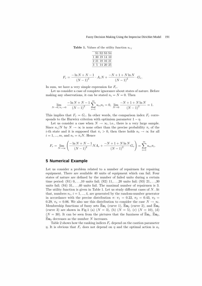
Table 1. Values of the utility function urj

S1 S2 S3 S4

1 30 19 14 10

2 21 18 16 21

3 5 14 20 25

Fr =− ln N + N − 1

(N − 1)2·ArN +

−N + 1 + N ln N

(N − 1)2·Gr.

In sum, we have a very simple expression for Fr.Let us consider a case of complete ignorance about states of nature. Before

making any observations, it can be stated ni = N = 0. Then

limN→0, ni→0

− ln N + N − 1

(N − 1)2

m∑

i=1

urini = 0, limN→0

−N + 1 + N ln N

(N − 1)2= 1.

This implies that Fr = Gr. In other words, the comparison index Fr corre-sponds to the Hurwicz criterion with optimism parameter 1− η.

Let us consider a case when N → ∞, i.e., there is a very large sample.Since ni/N by N → ∞ is none other than the precise probability πi of thei-th state and it is supposed that πi > 0, then there holds ni → ∞ for alli = 1, ..., m, and ni = πiN . Hence

Fr = limN→∞

(− ln N + N − 1

(N − 1)2NAr +

−N + 1 + N ln N

(N − 1)2Gr

)=

m∑

i=1

uriπi.

5 Numerical Example

Let us consider a problem related to a number of repairmen for repairingequipment. There are available 40 units of equipment which can fail. Fourstates of nature are defined by the number of failed units during a certaintime period: (S1) 0,. . . ,10 units fail; (S2) 11,. . . ,20 units fail; (S3) 21,. . . ,30units fail; (S4) 31,. . . ,40 units fail. The maximal number of repairmen is 3.The utility function is given in Table 1. Let us study different cases of N . Atthat, numbers ni, i = 1, ..., 4, are generated by the random-number generatorin accordance with the precise distribution π: π1 = 0.22, π2 = 0.43, π3 =0.29, π4 = 0.06. We also use this distribution to consider the case N → ∞.Membership functions of fuzzy sets Eu1 (curve 1), Eu2 (curve 2), and Eu3

(curve 3) are shown in Fig.1 (a) (N = 3), (b) (N = 5), (c) (N = 10), (d)(N = 30). It can be seen from the pictures that the fuzziness of Eu1, Eu2,Eu3 decreases as the number N increases.

Table 2 shows how the ranking indices Fr depend on the caution parameterη. It is obvious that Fr does not depend on η and the optimal action is a1


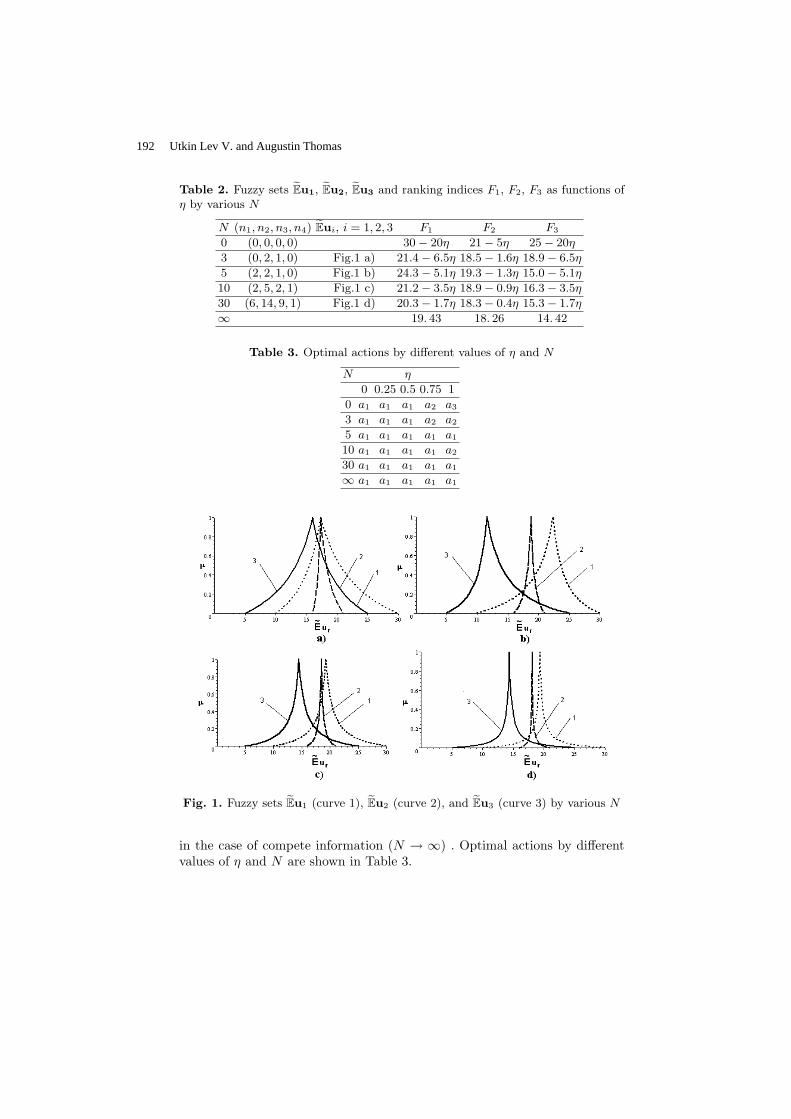
Table 2. Fuzzy sets Eu1, Eu2, Eu3 and ranking indices F1, F2, F3 as functions ofη by various N

N (n1, n2, n3, n4) Eui, i = 1, 2, 3 F1 F2 F3

0 (0, 0, 0, 0) 30− 20η 21− 5η 25− 20η

3 (0, 2, 1, 0) Fig.1 a) 21.4− 6.5η 18.5− 1.6η 18.9− 6.5η

5 (2, 2, 1, 0) Fig.1 b) 24.3− 5.1η 19.3− 1.3η 15.0− 5.1η

10 (2, 5, 2, 1) Fig.1 c) 21.2− 3.5η 18.9− 0.9η 16.3− 3.5η

30 (6, 14, 9, 1) Fig.1 d) 20.3− 1.7η 18.3− 0.4η 15.3− 1.7η

∞ 19. 43 18. 26 14. 42

Table 3. Optimal actions by different values of η and N

N η

0 0.25 0.5 0.75 1

0 a1 a1 a1 a2 a3

3 a1 a1 a1 a2 a2

5 a1 a1 a1 a1 a1

10 a1 a1 a1 a1 a2

30 a1 a1 a1 a1 a1

∞ a1 a1 a1 a1 a1

Fig. 1. Fuzzy sets Eu1 (curve 1), Eu2 (curve 2), and Eu3 (curve 3) by various N

in the case of compete information (N → ∞) . Optimal actions by differentvalues of η and N are shown in Table 3.

192 Utkin Lev V. and Augustin Thomas

6 Conclusion

The simplest decision problem has been studied in the paper. However, thefundamental ideas of this paper should be also applicable to more complexdecision problems, like multi-criteria decision making, decision problems withcombined objective and subjective initial information about states of nature,and decision problems with imprecise utilities. Another topic of further re-search is to extend the results obtained here to other optimality criteria, forexample, Walley’s maximality criterion. The problem can be also extended toa case of the randomized strategy instead of pure one considered in the paper.The proposed approach also can be applied to construction of fuzzy sets onthe basis of statistical observations.

References

1. Augustin T (2001) On decision making under ambiguous prior and samplinginformation. In: de Cooman G, Fine TL, Seidenfeld T (eds) Imprecise Proba-bilities and Their Applications. Proc. of the 2nd Int. Symposium ISIPTA’01,pages 9-16, Ithaca, USA, June

2. Augustin T (2002) Expected utility within a generalized concept of probability- a comprehensive framework for decision making under ambiguity. StatisticalPapers, 43:5-22

3. Campos LM and Gonzalez A (1989) A subjective approach for ranking fuzzynumbers. Fuzzy Sets and Systems, 29:145-153

4. Dubois D and Prade H (1988) Possibility Theory: An Approach to ComputerizedProcessing of Uncertainty. Plenum Press, New York

5. Kuznetsov VP (1991) Interval Statistical Models. Radio and Communication,Moscow. in Russian

6. Quaeghebeur E and de Cooman G (2003) Game-theoretic learning using theimprecise Dirichlet model. In: Bernard J-M, Seidenfeld T, Zaffalon M (eds) Proc.of the 3rd Int. Symposium on Imprecise Probabilities and Their Applications,ISIPTA’03, pages 450-464, Lugano, Switzerland, July. Carleton Scientific

7. Utkin LV (2003) Imprecise second-order hierarchical uncertainty model. In-ternational Journal of Uncertainty, Fuzziness and Knowledge-Based Systems,11(3):301-317

8. Utkin LV and Augustin T (2003) Decision making with imprecise second-order probabilities. In: Bernard J-M, Seidenfeld T, and Zaffalon M (eds) Proc.of the 3rd Int. Symposium on ImpreciseProbabilities and Their Applications,ISIPTA’03, pages 545-559, Lugano, Switzerland, July. Carleton Scientific

9. Walley P (1991) Statistical Reasoning with Imprecise Probabilities. Chapmanand Hall, London

10. Walley P (1996) Inferences from multinomial data: learning about a bag ofmarbles. Journal of the Royal Statistical Society, Series B, 58:3-57

11. Weichselberger K (2001) Elementare Grundbegriffe einer allgemeinerenWahrscheinlichkeitsrechnung, vol. I Intervallwahrscheinlichkeit als umfassendesKonzept. Physika, Heidelberg

12. Wilks S (1962) Mathematical Statistics. Wiley and Sons, New York


A Fuzzy Expert System for Predicting the Effect of Socio-economic Status on Noise-Induced Annoyance

Zaheeruddin1 and V.K Jain2

1 Department of Electrical Engineering, Faculty of Engineering and Technology, Jamia Millia Islamia (A Central University), New Delhi-110025, India [email protected]

2 School of Environmental Sciences, Jawaharlal Nehru University, New Mehrauli Road, New Delhi-110067, India [email protected]

Abstract. This paper proposes a novel approach for modelling noise-induced annoyance using fuzzy technique. The fuzzy approach offers a convenient way of representing the relationships between inputs and the outputs of a system in the form of simple IF-THEN rules. The annoyance in the present model is con-sidered as a function of noise level, its duration of occurrence, and socio-economic status of a person. The model has been implemented on Fuzzy Logic Toolbox of MATLAB using both Mamdani and Sugeno inference techniques. The results of the model are found to be in good agreement with the findings of World Health Organization (WHO) on noise-induced annoyance.

1 Introduction

The prominent adverse effects of noise pollution on human beings include loss of hearing, sleep disturbance, speech interference, reduction in work efficiency, and annoyance. Among these annoyance has been the most common term used to describe the communitys collective response to noise [1,2]. It should be clear, however, that annoyance is not merely a slight irritation, but is a manifestation of a significant deg-radation in the quality of life. The established definition by the World Health Organi-zation (WHO) says that health is a state of complete physical, mental and social well-being and not merely the absence of disease or infirmity [3]. Hence, according to this definition, annoyance is basically a health problem and may be defined as a feeling of displeasure associated with any agent or condition known or believed by an indi-vidual or a group to be adversely affecting them [3].

A number of studies have been conducted to examine the noise-annoyance rela-tionship [4-12]. Most of these studies have generally considered noise level and its duration of occurrence. However, social and economic factors, which may also have an important bearing on annoyance, have been neglected. It is, therefore, imperative that annoyance should be considered as a function of several parameters. The tradi-tional quantitative techniques have been the most effective tools for modelling the noise-annoyance relationship [13,14]. These techniques of systems modelling have

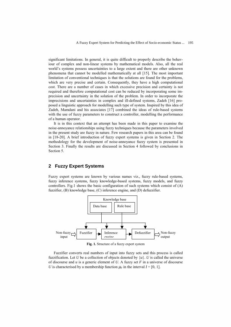
significant limitations. In general, it is quite difficult to properly describe the behav-iour of complex and non-linear systems by mathematical models. Also, all the real worlds systems possess uncertainties to a large extent and there are other unknown phenomena that cannot be modelled mathematically at all [15]. The most important limitation of conventional techniques is that the solutions are found for the problems, which are very precise and certain. Consequently, they have a high computational cost. There are a number of cases in which excessive precision and certainty is not required and therefore computational cost can be reduced by incorporating some im-precision and uncertainty in the solution of the problem. In order to incorporate the imprecisions and uncertainties in complex and ill-defined systems, Zadeh [16] pro-posed a linguistic approach for modelling such type of system. Inspired by this idea of Zadeh, Mamdani and his associates [17] combined the ideas of rule-based systems with the use of fuzzy parameters to construct a controller, modelling the performance of a human operator.

It is in this context that an attempt has been made in this paper to examine the noise-annoyance relationships using fuzzy techniques because the parameters involved in the present study are fuzzy in nature. Few research papers in this area can be found in [18-20]. A brief introduction of fuzzy expert systems is given in Section 2. The methodology for the development of noise-annoyance fuzzy system is presented in Section 3. Finally the results are discussed in Section 4 followed by conclusions in Section 5.

2 Fuzzy Expert Systems

Fuzzy expert systems are known by various names viz., fuzzy rule-based systems, fuzzy inference systems, fuzzy knowledge-based systems, fuzzy models, and fuzzy controllers. Fig.1 shows the basic configuration of such systems which consist of (A) fuzzifier, (B) knowledge base, (C) inference engine, and (D) defuzzifier.

Fig. 1. Structure of a fuzzy expert system Fuzzifier converts real numbers of input into fuzzy sets and this process is called

fuzzification. Let U be a collection of objects denoted by u. U is called the universe of discourse and u is a generic element of U. A fuzzy set F in a universe of discourse U is characterised by a membership function µF in the interval I = [0, 1].

Non-fuzzy input

Fuzzifier Inference engine

Defuzzifier Non-fuzzy output

Knowledge base

Data base Rule base

A Fuzzy Expert System for Predicting the Effect of Socio-economic Status ... 195

The knowledge base comprises a data base and a rule base. Membership functions of the fuzzy sets are contained in the data base. The rule base is a set of linguistic statements in the form of IF-THEN rules with antecedents and consequents respec-tively connected by AND operator. In general, a fuzzy rule-based system with multi-inputs single-output (MISO) can be represented in the following manner [21]:

IF X1 is B11 AND X2 is B12 AND … AND Xr is B1r THEN Y1 is D1 ALSO ….. ALSO IF X1 is Bi1 AND X2 is Bi2 AND … AND Xr is Bir THEN Ys is Ds,

where X1, , Xr are the input and Y1, , Ys are the output variables, Bij (i = 1, , m, j = 1, , r) and Dik (i = 1, , m, k = 1, , s) are fuzzy subsets of the universes of discourse U1, ... , Ur, and V1, . , Vs of X1, , Xr and Y1, , Ys respectively.

The inference engine is the kernel of a fuzzy rule based system, which employs IF-THEN rules from the rule base to infer the output by a fuzzy reasoning method. Zadeh [22-24] proposed the concept of possibility theory as the theoretical foundation for inference mechanism to deal with the uncertainty and imprecision in rule based sys-tems. The defuzzifier converts the fuzzy output obtained by inference engine into a non-fuzzy output real number domain and this process is called defuzzification. Though defuzzification seems to be the inverse of fuzzification but actually the maps need not be inverse of one another [25]. Among the several methods of defuzzifica-tion, the Centre of Area (COA) method is the most widely used.

3 Methodology

Noise-induced annoyance as a MISO system is shown in Fig. 2. It has three inputs and one output. Only those inputs, which affect the output to a large extent, have been selected. The most important input variables are noise level, duration of occurrence of noise, and the socio-economic status of the person. There is enough empirical evi-dence to suggest that a strong correlation exists between the socio-economic status of the person and noise-induced annoyance. Other factors such as gender, race, age, and motor-sidedness etc., which may influence the annoyance partially or marginally, have not been included. Inclusion of more inputs will increase the number of rules many fold and hence the complexity of the system increases.

Fuzzy System

Noise Level = X1

Annoyance = Y

Status = X3

Duration = X2

Fig. 2. Inputs and outputs of fuzzy system

196 Zaheeruddin and Jain V.K

The methodology for the development of the noise-annoyance fuzzy rule-based system involves the four steps: (1) Identification of the systems variables; (2) Deter-mination of the ranges of input and output variables; (3) Selection of the membership functions for various input and output variables; and (4) Formation of the set of lin-guistic rules.

The first and most important step in modelling is the identification of systems in-put and output variables. The relationships between them will specify the objective of the model. The second step is to determine the ranges of the input and output vari-ables. These variables in fuzzy modelling are defined as linguistic variables whose linguistic values are words or sentences in a natural or synthetic language. Table 1 shows the linguistic variables, their linguistic values and associated fuzzy intervals.

Table 1. Relations between inputs and outputs with their associated fuzzy values

S. No.

Systems Variables

Linguistic Variables

Linguistic Values Fuzzy Intervals

Low 30-60 dB(A) Medium 50-80 dB(A)

High 70-100 dB(A)

1.

Noise Level

Very High 90-120 dB(A) Very Short 0-20 Seconds

Short 10-40 Seconds Medium 30-70 Seconds

2.

Duration

Long 60-100 Seconds Very Poor 0-30 Point Scale

Poor 20-50 Point Scale Middle Class 40-70 Point Scale Upper Class 60-90 Point Scale

3.

Inputs

Status

Creamy Layer 80-100 Point Scale Negligible 0-20 %

Less 10-40 % Moderate 30-60 %

High 50-80 %

4.

Output

Annoyance

Extreme 70-100 % The next step is to express linguistic values in the form of fuzzy sets, which are rep-

resented by its membership functions. The membership functions are constructed from several basic functions such as piecewise linear functions, Gaussian distribution func-tion, sigmoid curve, quadratic and cubic polynomial curves. The triangular member-ship function is the simplest one and is commonly used due to its computational effi-ciency [26]. Membership functions for one input are shown in Fig. 3.

Finally, the relationships between inputs and output are represented in the form of IF-THEN rules. Two types of inference mechanisms are commonly used in fuzzy rule-based systems. The first was proposed by Mamdani [17]. In this case, both antece-dents and consequent predicates are fuzzy and IF-THEN rules are generally provided by an expert. The second was proposed by Takagi-Sugeno-Kang (TSK) and the mod-


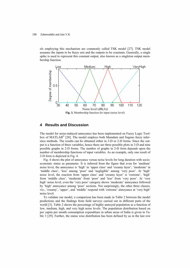
els employing this mechanism are commonly called TSK model [27]. TSK model assumes the inputs to be fuzzy sets and the outputs to be constants. Generally, a single spike is used to represent this constant output, also known as a singleton output mem-bership function.

Noise level (dB(A))

Fig. 3. Membership function for input (noise level)

4 Results and Discussion

The model for noise-induced annoyance has been implemented on Fuzzy Logic Tool-box of MATLAB® [28]. The model employs both Mamdani and Sugeno fuzzy infer-ence methods. The results can be obtained either in 3-D or 2-D forms. Since the out-put is a function of three variables, hence there are three possible plots in 3-D and nine possible graphs in 2-D forms. The number of graphs in 2-D form depends upon the number of membership functions of input variables. As an example, only one result of 2-D form is depicted in Fig. 4.

Fig. 4 shows the plot of annoyance versus noise levels for long duration with socio-economic status as parameter. It is inferred from the figure that even for medium noise level, the annoyance is high in upper class and creamy layer, moderate in middle class, less among poor and negligible among very poor. At high noise level, the reaction from upper class and creamy layer is extreme, high from middle class, moderate from poor and less from very poor. At very high noise level, even the very poor category shows moderate annoyance followed by high annoyance among poor sections. Not surprisingly, the other three classes, viz., creamy, upper, and middle respond with extreme annoyance at very high noise level.

To validate our model, a comparison has been made in Table 2 between the model predictions and the findings from field surveys carried out in different parts of the world [3]. Table 2 shows the percentage of highly annoyed population as a function of low, medium, high, and very high noise levels. The population distribution based on per capita per month consumption expenditure in urban areas of India is given in Ta-ble 3 [29]. Further, the status wise distribution has been defined by us in the last row


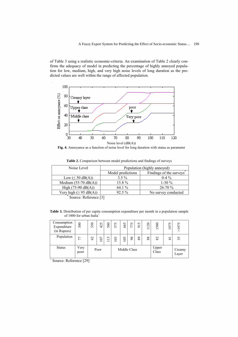
of Table 3 using a realistic economic-criteria. An examination of Table 2 clearly con-firms the adequacy of model in predicting the percentage of highly annoyed popula-tion for low, medium, high, and very high noise levels of long duration as the pre-dicted values are well within the range of affected population.

Noise level (dB(A))

Fig. 4. Annoyance as a function of noise level for long duration with status as parameter

Table 2. Comparison between model predictions and findings of surveys

Population (highly annoyed) Noise Level Model predictions Findings of the surveys*

Low (≤ 50 dB(A)) 3.5 % 0-4 % Medium (55-70 dB(A)) 15.8 % 1-30 %

High (75-90 dB(A)) 64.1 % 26-70 % Very high (≥ 95 dB(A)) 92.5 % No survey conducted

* Source: Reference [3]

Table 3. Distribution of per capita consumption expenditure per month in a population sample of 1000 for urban India+

Consumption Expenditure (in Rupees)

300

350

425

500

575

665

775

915

1120

1500

1975

>197

5

Population

77

62

107

113

103

105 98

89

88

82

41

35

Status Very poor Poor Middle Class Upper

Class

Creamy Layer

+ Source: Reference [29]


5 Conclusion

The main thrust of the present work has been to develop a fuzzy rule-based system for the prediction of noise-induced annoyance. The annoyance has been modelled as a function of noise levels, their durations of occurrence, and socio-economic status of the population. The fuzzy model has been implemented using both Mamdani and Sugeno inference techniques. The results with the proposed model are in good agree-ment with the findings of field surveys conducted in different parts of the world. The model clearly brings out the salient feature of the surveys concerning the variation of annoyance with noise levels while taking into account the status as one of the most important parameters.

References

1. Suter, A.H.: Noise and its effects. This is available online at http://www.nonoise.org/library/suter/suter.html. (1991)

2. EPA (ed.): Noise Effects Handbook. [online]. Available: http://www.nonoise.org/library/handbook/handbook.html. U.S. Environmental Protection Agency, Florida (1981)

3. Berglund, B., Lindvall, T., (eds.): Community Noise. [online]. Available: http://www.nonoise.org/library/whonoise.html. Document prepared for WHO, Stockholm, Sweden (1995)

4. Miedema, H.M.E.: Annoyance caused by two noise sources. J. Sound and Vibration. 98 (1985) 592-595

5. Fidell, S., Barber, D.S. Barber, Schultz, T.J.: Updating a dosage-effect relationship for the prevalence of annoyance due to general transportation noise. J. Acoust. Soc. Am. 89 (1991) 221-223

6. Miedema, H.M.E., Vos, H.: Exposure response relationship for transportation noise. J. Acoust. Soc. Am. 104 (1998) 3432-3445

7. Buchta, E., Vos, J.: A field survey on the annoyance caused by sounds from large firearms and road traffic. J. Acoust. Soc. Am. 104 (1998) 2890-2902

8. Green, D.M., Fidell, S.: Variability in the criterion for reporting annoyance in community noise surveys. J. Acoust. Soc. Am. 89 (1991) 234-243

9. Hall, F., Birnie, S., Taylor, S.M., Palmer, J.: Direct comparison of community response to road traffic noise and to aircraft noise. J. Acoust. Soc. Am. 70 (1981) 1690-1698

10. Fields, J.M.: A quantitative summary of non-acoustical variables effects on reactions to environmental noise. In: Busch-Vishniac, I. (ed.): National Conference on Noise Control Engineering: Reducing the Annoyance of Noise, University of Texas (1990)

11. U. S. Environmental Protection Agency. An Assessment of Noise Concern in Other Na-tions. Rep. No. NTID 300.6, Vol. 1 (1971)

12. Denver Department of Environmental Health: Denver Noise Survey. [online]. Available: http://www.nonoise.org/library/denver/survey.html. (1997)

13. Arana, M., Garcia, A.: A social survey on the effects of environmental noise on the resi-dents of Pamplona, Spain. Applied Acoustics 53 (1998) 245-253

14. Pandya, G.H.: Urban noiseA need for acoustic planning. Environmental Monitoring and Assessment. 67 (2001) 379-388


http://www.nonoise.org/library/suter/suter.html

15. Emami, M.R., Turksen, I.B., Goldenberg, A.A.: Development of a Systematic Methodology of Fuzzy Logic Modelling. IEEE Transactions on Fuzzy Systems 6(1998) 346-361

16. Zadeh, L.A.: Outline of a new approach to the analysis of complex systems and decision processes. IEEE Transactions on Syst., Man, and Cyber. SMC-3 (1973) 28-44

17. Mamdani, E.H., Assilian, S.: An experiment in linguistic synthesis with a fuzzy logic con-troller. Intern. J. of Man-Machine Studies 7 (1975) 1-13

18. Zaheeruddin, Singh, G.V., Jain, V.K.: Fuzzy Modelling of Human Work Efficiency in Noisy Environment. Proc. The IEEE Internat. Conf. Fuzzy Systems, Vol. 1 (2003) 120-124

19. Zaheeruddin, Jain, V.K.: A Fuzzy Approach for Modelling the Effects of Noise Pollution on Human Performance. Internat. Journal of Advance Computational Intelligence and Intel-ligent Informatics. 8(2004) to appear

20. Zaheeruddin, Jain V.K.: An Intelligent System for Noise-induced Hearing Loss. Proc. of Intern. Conf. Intelligent Sensing and Information Processing (ICISIP 2004), Chennai, In-dia, January 4-7, (2004) 379-384

21. Yager, R.R., Filev, D.P.: Essentials of Fuzzy Modeling and Control. John Wiley & Sons, Inc. New York (1994)

22. Zadeh, L.A.: Fuzzy logic and approximate reasoning. Synthese. 30 (1975) 407-428 23. Zadeh, L.A.: The concept of linguistic variable and its application to approximate reason-

ing. Information Sciences. 1,2,3 (1975) 199-249, 301-357, 43-80 24. Zadeh, L.A.: Fuzzy sets as a basis for a theory of possibility. Fuzzy Sets and Systems. 1

(1978) 3-28 25. Lygeros, J.: A formal approach to fuzzy modeling. IEEE Transactions on Fuzzy Systems. 5

(1997) 317-327 26. Arslan, A., Kaya, M.: Determination of fuzzy logic membership functions using genetic

algorithms. Fuzzy Sets and Systems. 118 (2001) 297-306 27. Takagi, T., Sugeno, M: Fuzzy Identification of Systems and its Applications to Modelling

and Control. IEEE Trans. Syst., Man, and Cyber. 15 (1985) 116-132 28. Fuzzy Logic Toolbox for use with MATLAB®. The MathWorks Inc., USA (2000) 29. Department of Statistics (Government of India). National Sample Survey: Level and Pattern

of Consumer Expenditure in India, NSS Report No. 457, 1999-2000


The knowledge representation model in fuzzy expert systems provided by computing with words and PRUF language

V.I. Glova, Dr.Sci., I.V. Anikin, PhD, A.S. Katasev, p.-gr.st., O.N. Pheok-tistov, p.-gr.st.

Department CSIS, Kazan State Technical University named after A.N. Tu-polev, e-mail: [email protected], [email protected]

ABSTRACT. We considered the problem of knowledge representation and processing in fuzzy expert systems, also their application in economics. We developed the representation and processing model of expert knowl-edge in expert systems provided by computing with words and PRUF lan-guage. Authors introduced the architecture of PRUF language translator, which is developed as one of the expert system modules. Provided by ex-tended Backus-Naur forms we described the basic PRUF language structures.

Introduction

The solving of many problems of optimization, diagnostics, prediction and functional business component modelling is reviewed in a new fashion at present because of rapid development of intelligent information tech-nologies. More often we must solve these problems in conditions of fuzzi-ness, uncertainty and incompleteness of source information. In this situa-tion there is a critical question of using such methods of information processing, which are suitable for functioning in these conditions.

The fuzzy sets theory offers one of possible methods of linguistic uncer-tainty processing, qualitative conceptions, which are used by people in everyday life [1],[2]. Using the fuzzy sets theory is more efficiently in case of need of attraction to task solution process sufficiently large volume of subjective knowledge, which can describe facts, goals and heuristic de-vices of tasks solution. This situation arises very often during solving of financial analysis tasks, investment planning, technical analysis and stock market prediction, dynamic scheduling and business-process modelling [3],[4].

One of more perspective directions of solving these tasks is attraction of computer technology for this process in form of decision-support systems (DSS) and expert systems.

The production models of knowledge representation in expert systems

Expert system (ES) is a computer system designed for solving of diffi-cult formalized tasks on basis of knowledge base which reflects the collec-tive operational experience of experts in research area, and for solving process explanation of task for expert system user.

Expert system is an instrument which accelerates expert’s intelligent ca-pacities and must execute next functions [5]: consultant for novice and unprofessional users; assistant because of necessity of analysis by expert different variants of

decision-making; expert’s partner on questions, which concern to knowledge sources from

adjacent areas. Of one's own structure any ES consists of two builders [5]: knowledge base (KB), which stores knowledge about data domain; software component of access and knowledge processing, which con-

sists of inferential mechanism, knowledge acquisition mechanism, ex-planation of receiving results and intelligent interface. The central components of any ES are knowledge base and inference

engine. Therefore, functioning of ES as a whole depends on formalization, representation and processing expert’s knowledge about data domain.

The production models and their generalizations are sufficiently popular models of procedural knowledge representation in ES as the most conven-ient for creating output mechanisms [6]. The declarative knowledge about problem area in ES are better represented with help of semantic networks [7]. View the production rules as a model of knowledge formalization in ES.

In general, the production rules have next form: IF А1 AND/OR A2 … AND/OR An THEN B1, B2, B3 … Bm

where A1,…,An – premises set, and B1,…,Bm – conclusions set, which take place on condition that executed premises set.

The completeness and consistency of these rules is achieved at the ex-pense of the ES adjustment on the simulation systems together with ex-perts.

For conclusion on knowledge, which are presented in form of produc-tion rules, the resolution principle is used [8].

The knowledge representation model in fuzzy expert systems ... 203

The fuzziness and qualitative of initial data, informal methods of tasks solution and attainable aims results in necessity of using fuzzy production rules, which are represented in form of Mamdani and Sugeno models as well as their special cases – Cykamoto and Larsen models [9],[10].

In Mamdani model the production rules have next form: IF A1 is 1

~A AND/OR A2 is 2~A … AND/OR An is nA~

THEN B1 is 1~B ,…, Bm is mB~

where 1~A ,…, nA~ , mBB ~,...,~

1 – fuzzy restrictions on values of variables A1,…,An,B1,….,Bm, which are specified as fuzzy variables – values of re-spective linguistic variables.

In Sugeno model the production rules have next form: IF A1 is 1

~A AND/OR A2 is 2~A … AND/OR An is nA~

THEN ),...,( 1 nAAfz = where f – some function of arguments A1,…,An.

The conclusion on Mamdani and Sugeno fuzzy models is used in fuzzy expert systems and fuzzy control systems, including in expert systems in different economics areas [11],[12],[13]. Using the fuzzy control systems allows considerably enhance stability of their functioning under existing conditions (noises, fuzziness, lack of initial information, fuzziness of at-tainable aims), reduce the computational complexity of obtained decision, more softy adapt for environment fluctuation.

The representation and processing of expert knowledge provided by computing with words and PRUF language

The tasks solution efficacy, which solve the expert systems, is defined by expert’s level of proficiency by quality of ES finalizing on the systems of simulation as well as capability of using model for knowledge represen-tation in knowledge base of expert system on expert’s knowledge formal-ization.

At present the most prevailing knowledge representation models can not often satisfy all expert’s requirements. His knowledge passes through the prism of those restrictions, which are in concrete model. As a result the question of building the model, which would allow an expert to formulate one's own knowledge in convenient form, on the near natural language, is very actual.

A number of preference on expert’s knowledge formalization, in com-parison with existent, offer the models of computing with words technol-ogy and PRUF language [14],[15]. The main their virtue is a capability of

204 Glova V.I. et al.

expert knowledge representation on the near natural language as a canoni-cal forms, in which is made processing. The main purpose of PRUF is a truth definition of natural language expressions in desired conditions.

Provided by PRUF language L.A. Zade introduces the correct language constructions, which can be represented and processed [16]. The basic constituent of these constructions are statement sets and restrictions, which are imposed upon these statements. The canonical form of writing such expert expression is represented in form:

X isr R where X is a statement, R is a restriction, which is laided on possible val-ues of X, isr is a variable-bunch, which defines the type of restriction.

Provided by PRUF language, which is under considered by L.A. Zade, are used such constituent language structures as 1. Fuzzy and linguistic variables, permissing to formalize the fuzzy con-

ceptions and linguistic categories, which are used by expert during statements forming. For example «FINANCIAL PERFORMANCE» = POOR, SATISFACTORY, GOOD.

2. Fuzzy modifiers, permissing to modify the semantics of entered restric-tions by given way and generate the extended term-set of linguistic vari-able values from base terms set (VERY POOR FINANCIAL PERFORMANCE, NOT VERY LOW NET PROFIT RATIO and so on).

3. Fuzzyfiers, permissing to fuzzyfy crisp and fuzzy given restrictions, covered on controlled variables (MORE-LESS SATISFACTORY FINANCIAL PERFORMANCE, APPROXIMATELY ZERO NET PROFIT RATIO and so on).

4. Limiters (possible, probabilistic and so on). 5. Bunchs (AND, OR)

The base types of restrictions, which are viewed by L.A. Zade, are next: 1. Possible value (is). 2. Probabilistic restriction (isp). 3. Restriction by random set (isrs). 4. Restriction given in form fuzzy graph (isfg). 5. Restriction by linguistic probability (ispv). 6. Restriction by linguistic truth (istv). 7. Restriction of commonness (isu).

Provided by these restrictions expert can form the statements, which is refered to problem area as well as appreciate the truth degree of natural language expressions in the given situation. In practice, these expressions can join with each other controlled variables and laid as data domain de-scription to knowledge base of expert system. Using this approach will al-


low a great extent increase the expert’s possibility on forming of expert system knowledge base.

Review the examples of expert’s statements, which can be formalized provided by PRUF language.

Example 1. «Fully probably that in the near future oil price will appre-ciably rise».

In the terms of PRUF language this expression can be written in the fol-lowing way:

LV_Probability LV_Space of time(O_Space of time) is FV_Near future and_p LV_Change of oil price (O_Change of oil price) is M_Appreciably(FV_Rise) isp M_Fully(FV_Probably)

Here LV_Probability, LV_Space of time, LV_Change of oil price – lin-guistic variables, FV_Probably, FV_Near future, FV_Rise – their values (fuzzy variables), M_Appreciably, M_Fully – modifiers, O_ Space of time, O_ Change of oil price – objects.

There is the hidden linguistic variable LV_Probability in this expression and her value FV_Probably (fuzzy variable).

Example 2. «If demand for commodity will be low and expenses will be small, then in the near future the price of commodity will fall».

This expression can be written in the following way: IF LV_Demand(O_Commodity) is FV_Low AND LV_Expenses(О_Commodity) is FV_Small THEN LV_Period of price change(О_Commodity) is FV_Near future AND LV_Change of price(О_Commodity) is FV_Fall In this case there are four linguistic variables in expression –

LV_Demand, LV_Expenses, LV_Period of price change, LV_Change of price, four fuzzy variables – FV_Low, FV_Small, FV_Near future, FV_Fall, as well as object O_Commodity, his characteristic we must evaluate.

The semantics of conceptions, which are used in expressions, is defined in EDF-tables in form of membership functions.

The creation of PRUF language translator for expert systems

We developed the PRUF language translator for his using in inference engine of expert systems, including in expert systems in different econom-ics fields.

The vocabulary and syntax of more widespread language structures of PRUF is described by authors provided by extended Backus-Naur forms,


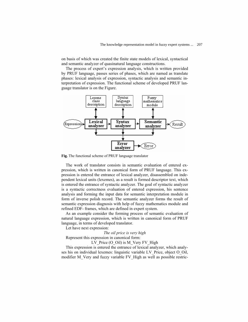
on basis of which was created the finite state models of lexical, syntactical and semantic analyzer of quasinatural language constructions.

The process of expert’s expression analysis, which is written provided by PRUF language, passes series of phases, which are named as translate phases: lexical analysis of expression, syntactic analysis and semantic in-terpretation of expression. The functional scheme of developed PRUF lan-guage translator is on the Figure.

Fig. The functional scheme of PRUF language translator

The work of translator consists in semantic evaluation of entered ex-pression, which is written in canonical form of PRUF language. This ex-pression is entered the entrance of lexical analyzer, disassembled on inde-pendent lexical units (lexemes), as a result is formed descriptor text, which is entered the entrance of syntactic analyzer. The goal of syntactic analyzer is a syntactic correctness evaluation of entered expression, his sentence analysis and forming the input data for semantic interpretation module in form of inverse polish record. The semantic analyzer forms the result of semantic expression diagnosis with help of fuzzy mathematics module and refined EDF- frames, which are defined in expert system.

As an example consider the forming process of semantic evaluation of natural language expression, which is written in canonical form of PRUF language, in terms of developed translator.

Let have next expression: The oil price is very high

Represent this expression in canonical form: LV_Price (O_Oil) is M_Very FV_High

This expression is entered the entrance of lexical analyzer, which analy-ses his on individual lexemes: linguistic variable LV_Price, object O_Oil, modifier M_Very and fuzzy variable FV_High as well as possible restric-


tion is and brackets. The descriptor tables are formed from these lexemes. Each lexeme is written as descriptor as xx xxx. First two numbers are number of descriptor table, which stores the lexeme. Last three numbers are order number of lexeme, which is stored in this table.

The set of these descriptor lexemes are descriptor text, which is entered the entrance of syntax analyzer. Then this text is transformed to more con-venient form for working. In our example we have:

<lv>’(’<o>’)’<r><m><fv> The syntax analyzer solves such tasks as:

defines the syntactical correctness of expression on basis of well-known syntactically correct templates:

transforms this expression into inverse polish record as <o><lv><fv><m><r>

which is entered the entrance of semantic analyzer. The analysis of given set in semantic analyzer allows identically define

his numerical semantic evaluation of truth on condition of formalization of semantic meaning for all composite elements of given construction. This formalization is realized provided by developed fuzzy mathematics library.

The translator realization represents the special-purpose library, which will be connected up to external with respect to this library expert system.

Using of this translator will allow to experts form more full description of knowledge domain on solving of difficult formalized tasks.

References

[1] Altunin A.E., Semuhin M.V. The models and algorithms of de-cision-making in fuzzy conditions: Monograph. Tyumen: Pub-lisher by Tyumen State University, 2000. – 352 p.

[2] Frolov U.V. The intellectual systems and management decisions. - Moscow: MSPU, 2000. – 294 p.

[3] The decision-making models in terms of linguistic variable / A.N. Borisov and others. – Riga: Zinatne, 1982.

[4] Nedosekin A.O. The methodological foundations for modeling of financing activities with help of fuzzy-multiple descriptions. – Saint-Petersburg, 2003.

[5] Telnov U.F. The intellectual information systems in economics: Tutorial. – М.: SYNTEG, 1999. – 216 p.

[6] Gavrilova T.A., Horoshevsky V.F. The knowledge bases of in-tellectual systems. – St. Petersburg.: Piter, 2001. – 384 p.


[7] Marenko V.A. The methods of knowledge representation in ex-pert systems //The mathematical structures and modelling. – 2001. – 8. – P.34–39

[8] P. Jackson. Introduction to expert systems. M: Williams, 2001. [9] V.V. Kruglov, M.I. Dli, R.U.Golunov. Fuzzy logic and artificial

neuron networks. M.: Physmatlit, 2001. [10] Averkin A.N., Batyrshin I.Z., Blishun A.F. and others. Fuzzy

sets in management models and artificial intelligence. // Under edit. Pospelov D.A. М.: Science, 1986. 311 p.

[11] Dourra H., Siy P. Investment using technical analysis and fuzzy logic. // Fuzzy Sets and Systems, – 127, 2002.

[12] Nedovic L., Devedgic V. Expert system in finance - a cross-section of the field. // Expert Systems with Applications, – 23, 2002.

[13] Zopounidis C., Doumpos M., Matsatsinis M. On the use of knowledge-based decisions support systems in financial man-agement: A survey. // Decision Support Systems, – 20, 1997.

[14] L.A. Zadeh. Fuzzy Logic = Computing with words // IEEE Transactions on fuzzy systems, Vol. 4, N. 2, 1996.

[15] L.A. Zadeh. PRUF – A meaning representation language for natural languages//Int. J. Man-Mach. Studies, vol. 10, 1978.

[16] L.A. Zadeh. Test-score semantics for natural languages and meaning representation via PRUF//Empirical Semantics, B. Reiger, Ed., W.Germany: Brockmeyer, 1981.


Construction of Incremental Fuzzy Deci-sion Tree

Arkady Borisov* and Gulnara Bikesheva** *Riga Technical University”, 1Meza Str., Professor, Dr.habil.sci.comp. E-mail: [email protected] **Joint-stock company DATI, Ganibu-dambis Str. 17a, Programmer, Master of

Computer Science E-mail: [email protected]

Abstract

This paper considers algorithms for incremental induction of fuzzy decision trees. Incremental learning ability is very important for solving real-world problems for the following reasons. When new examples ap-pear, one can make some revision on the trained system and incorporate new knowledge. Modifying a trained system takes much less time than building a new system. The algorithm presented combines three properties: it generates decision trees which are able to classify and generalize the data; it utilizes fuzzy logic that allows it to operate with indistinct concepts characteristic to human reasoning; and it is incremental, which enables it to use new data without building a new tree.

The paper also describes incremental algorithms for fuzzy induction of decision trees using classical logic. Then this algorithm is modified for use in indistinct logic. It has a variety of modifications. It allows working with both numeric and symbolic information, processing both inconsistent and incomplete data. An example of construction of an incremental fuzzy deci-sion tree is considered in detail to illustrate the new algorithms potential.

Key words: fuzzy decision tree, classification, incremental learning,

non-incremental learning, tree induction, fuzzy logic

1. Introduction

Decision-tree algorithms provide one of the most popular methodologies for symbolic knowledge acquisition. The popularity of decision trees is based on such advantages, as speed of construction and ease of usage at

classification. Because of the natural interpretation of knowledge, sym-bolic decision trees can easily be translated into a set of rules suitable for use in rule-based systems.

Today, a great number of algorithms for automatic construction of deci-sion trees are in existence. Most of them are based on well-known algo-rithms ID3 and CART which allow working with both symbolic and con-tinuous-valued attributes. In many practical applications, the data used are inherently of imprecise and subjective nature. A popular approach to cap-ture this vagueness of information is the use of fuzzy logic, going back to Zadeh [7]. To combine the advantages of decision trees and fuzzy logic [8], the concept of a decision tree has been supplemented with fuzzy logic, and there is a set of algorithms creating such trees [6]. Unlike approaches based on classical logic, a fuzzy decision tree is able to deal with a degree of truth in classification of new examples.

To construct a fuzzy decision tree, several algorithms can be used. They differ in the search criteria employed to find the most important attribute. Say, Zeidler [1] applies traditional entropy measure borrowed from the pa-pers of Quinlan [12]. Wang [9] describes maximum information gain that is based on linguistic information. In [10] fuzzy entropy measure intro-duced by Kosko [11] is used to evaluate the effectiveness of attributes. All the aforementioned algorithms suffer from one drawback: they are unable to work in the online mode.

Moreover, the present algorithms for induction of fuzzy decision trees are non-incremental. These algorithms do not allow adopting the received results to the new data. The incremental algorithms allow re-structuring the existing decision tree for incorporation of new data, which enables one to essentially reduce calculation costs.

This paper presents a new classification algorithm based on Zeidler’s works. The algorithm combines three properties: it generates decision trees which have the ability to classify and generalize the data; it utilizes fuzzy logic which enables us to deal with vague concepts characteristic of human reasoning; and it is incremental which allows one to use new data, without building a new tree.

This paper consists of the following parts: - necessary definitions from the fuzzy logic theory and decision trees; - the concept of fuzzy decision tree based on ID3; - description of incremental induction, based on Utgoff [3,4,5]; - an algorithm that combines advantages of fuzzy decision tree and in-

cremental approach; - an illustrative example of fuzzy decision tree construction and restruc-

turing. The paper ends with conclusions and references.

Construction of Incremental Fuzzy Decision Tree 211

2. Fuzzy Sets and Fuzzy Linguistic Variables

Set and element are two basic notions of the set theory. In the classical

set theory, an element either belongs to a certain set or it doesn’t. There-fore, a set can be defined by a two-valued characteristic function U → 0,1, where U is the universe of discourse. In the fuzzy set theory, a fuzzy subset of the universe of discourse U is described by a membership func-tion µv(V): U→[0,1] which represents a degree by which Uu∈ belongs to set v.

The concept of the fuzzy linguistic variable is used to describe objects and phenomena using fuzzy sets. The meaning of the linguistic term is de-fined by a fuzzy set, which in its turn is defined by its membership func-tion.

An atomic fuzzy proposition (often called a fuzzy restriction) is defined as [V is A], where V- is a fuzzy variable and v – is a fuzzy term from its linguistic domain. The classical rule If then in fuzzy logic may be repre-sented as

R= if V1 is A1 and … Vj is Aj then D is AD A fuzzy rule-based system is a set of certain fuzzy rules along with

special inference procedures.

3. Decision Trees

A decision tree is a representation of rules in a hierarchical, consecutive structure where each object has its corresponding unique node giving a decision. Several algorithms have been developed in order to ensure the construction of decision trees and their use for the classification task. The ID3 and CART are the two most important discriminative learning algorithms based on recursive partitioning.

An important property of these algorithms is that they attempt to mini-mize the size of the tree by optimizing some quality measure. ID3 assumes discrete domains with small cardinalities. CART enables one to use con-tinuous attributes. Now we will consider the ID3 algorithm, which will later be modified to a fuzzy decision tree.

1. Compute the information content at node N given by

212 Borisov Arkady and Bikesheva Gulnara

∑=

⋅−=||

1)log(

C

iii

N ppInfo , (1)

where C is the set of decisions, and pi is the probability that a training example in the node represents class i.

2. For each attribute ai not appearing on the path to N and for each of its domain values aij, compute the information content ijaNInfo | in a child node restricted by the additional condition ai = aij.

3. Select the attribute ia maximizing the information gain

∑ ⋅−=||

| )(i

ij

D

j

aNj

N InfowInfoGain

(2)

where wj is the relative weight of examples in the child node following aij condition to the total number of examples in N, and Di is the symbolic domain of the attribute.

4. Split node N using the selected attribute.

4. Fuzzy Decision Trees

Fuzzy decision trees differ from the traditional ID3 algorithm in the following points [1]:

1. There is a membership grade µ (0 ≤ µ ≤ 1) for all input examples 2. The algorithm does not only create a leaf node if all data belong to the

same class but also in the following cases: - if the proportion of a data set of class Ck is greater than or equal

to an assigned threshold (prepruning of subsequent nodes because “nearly all” data belong to the same class),

- if the number of elements in a data set is less than an assigned threshold (prepruning because of “numerical tininess”of the set) or

- if there are no more attributes for classification (in ID3 there is a null class for this leaf node)

3. More than one class name may be assigned to the leaf node (a real advantage of a fuzzy decision tree).

4. Each attribute is considered as a linguistic variable. The membership function for each attribute is user-defined or can be calculated from the boundary points of the interval using the following algorithm:

- Values of the attribute are divided into intervals and cut points are defined.

- For representing membership functions we choose the trapezoi-dal one. Storing these functions is simple, because four corner points (A, B, C, D) are sufficient description.


- Start and end points for each range where the membership grade equals 1 (B and C)

- Start and end points for each range where the membership grade equals 0 (A and D)

For fuzzy decision trees we use ||

),(T

TCfrec j instead of ip in calculat-

ing the information content of the node in formulas (1) and (2), where || T is the sum of membership functions of all classes of training set Т and

),( TCfrec j is the sum of membership functions of class jC of training set Т.

5. Incremental Induction

Suppose we have a tree t constructed from a training set λ. Now we get some new information and build a new tree t' that is based on a new training set λ’ containing λ and a couple of new training examples. In comparing the two trees, two things may occur: first, the annotated class distribution may change, and second, the structure of the tree may change.

To be able to change the test that is installed in a decision node, one needs to maintain information in that node to provide the basis for evaluating the quality of each possible test. For each possible test, the fre-quency counts for each outcome-class combination are kept and updated as necessary. For example, the test (color =blue) contains 5 examples from the training set: two of them belong to class 1, three – to class 2. Hence, in this node we keep two frequencies 2/5 and 3/5.

As the first step in reconstructing of the tree, we add a new exam-ple without changing the structure of the tree. When an example is to be incorporated into an empty tree, the tree is replaced by a “leaf” node that indicates the class of the leaf, and the example is saved in the leaf node. Whenever a new example is to be incorporated, the branches of the tree are followed as far as possible according to the values in the example. If the example belongs to the same class as the leaf, the example is simply added to the set of examples saved in the leaf node. If the example has a class la-bel different from the leaf, the algorithm attempts to turn the leaf into a de-cision node, picking the best test according to the test-selection metric. The examples saved in the node that has just been converted from a leaf node into a decision node are then incorporated recursively by sending each one down its proper branch according to the new test. Thus, an example can be added to a node, and it will work its way down the tree to a leaf, possibly sprouting branches at leaves as it moves down the tree.


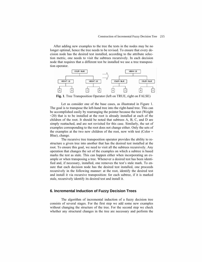
After adding new examples to the tree the tests in the nodes may be no longer optimal, hence the tree needs to be revised. To ensure that every de-cision node has the desired test installed, according to the attribute selec-tion metric, one needs to visit the subtrees recursively. In each decision node that requires that a different test be installed we use a tree transposi-tion operator.

Fig. 1. Tree Transposition Operator (left on TRUE, right on FALSE)

Let us consider one of the base cases, as illustrated in Figure 1.

The goal is to transpose the left-hand tree into the right-hand tree. This can be accomplished easily by rearranging the pointer because the test (Weight <20) that is to be installed at the root is already installed at each of the children of the root. It should be noted that subtrees A, B, C, and D are simply reattached, and are not revisited for this case. Similarly, the set of examples corresponding to the root does not change either. Only the sets of the examples at the two new children of the root, now with test (Color = Blue), change.

The recursive tree transposition operator provides the ability to re-structure a given tree into another that has the desired test installed at the root. To ensure this goal, we need to visit all the subtrees recursively. Any operation that changes the set of the examples on which a subtree is based marks the test as stale. This can happen either when incorporating an ex-ample or when transposing a tree. Whenever a desired test has been identi-fied and, if necessary, installed, one removes the test’s stale mark. To en-sure that each decision node has the desired test installed, one proceeds recursively in the following manner: at the root, identify the desired test and install it via recursive transposition: for each subtree, if it is marked stale, recursively identify its desired test and install it.

6. Incremental Induction of Fuzzy Decision Trees

The algorithm of incremental induction of a fuzzy decision tree consists of several stages. For the first step we add some new examples without changing the structure of the tree. For the second step we check whether any structural changes in the tree are necessary and perform the


necessary changes in the tree. This procedure determines the best tests for decision nodes. We use a transposition operator for swapping nodes in a subtree so as to get the desired conditions on the top node of the subtree. Additionally we use the procedure for classification of new examples, which do not enter into the tree.

This algorithm can have several modifications depending on the criteria of estimation of quality in the decision nodes. In our case we use information Gain. The best test is one with the maximal value of informa-tion Gain. If it is necessary to add some new examples in the tree, the algo-rithm can restructure the tree after each example. If there are quite a few new examples, it is expedient to restructure the tree after adding all the new examples or part of them. Upon presentation of a new training exam-ple, one can decide whether or not to incorporate the training example into the tree. We can use the ability of the already existing tree to correctly classify the new example for making the decision.

7. An Example of Creating the Incremental Fuzzy Deci-

sion Tree Our algorithm is illustrated with data from [1,2]. We have the following attributes: height; weight; hair color (blond,

black, and red) and two classes C1 and C2. µ (0 ≤ µ ≤ 1) – is the class membership grade of an example. Data T with µ are given in Table 1. Table 1. Data T num-

ber 1 2 3 4 5 6 7 8

height 160

180

170

175

160

175

165

180

weight

60 80 75 60

75 60

60 70

hair color

blond

black

black

red

Black

red

Blond

blond

class C1 C2 C2 C1

C2 C2

C2 C1

µ 1 0,8 0,2 0,7

1 0,3

1 0,5

We only use the first four examples for constructing a fuzzy decision

tree on the basis of the fuzzy ID3 algorithm suggested.


First, the attribute values height and weight are arranged in the as-cending order and the cut points are determined. In our example we have one or two possible cut points between data of different classes.

Table 2. Data sorted by Height Cut points: 1 2 number 1 3 4 2 height 1

60 1

70 17

5 18

0 class C

1 C

2 C1 C2

µ 1 0,2

0,7 0,8

Table 3. Data sorted by weight

Cut points: 1 number 1 4 3 2 weight 6

0 6

0 75 80

class C1

C1

C2 C2

µ 1 0,7

0,2 0,8

To construct the fuzzy decision tree, we do not calculate the number of examples for class 1 and class 2, we count the sum of class membership grades of the examples:

freq(C1, T) = 1+0.7 = 1.7 freq(C2, T) = 0.8 + 0.2 = 1 ||T| = 1 +0.8 +0.2 +0.7 = 2.7 Info(T) = -1.7/2.7 * log2(1.7/2.7) - 1/2.7 *log2(1/2.7) = 0.95 For the hair color attribute we obtain this: Info(Hair_color, T) = 0 Gain(Hair_color, T)= Info(T) – Info(Hair_color, T) = 0.95- 0 = 0.95 For the height and weight attributes, we find discretization with the can-

didate cut points and calculate the information gains: Info (Height, Т, Cut_point1) = 0.843 Gain (Height, Т, Cut_point1)=

0.128 Info (Height, Т, Cut_point2) = 0.342 Gain (Height, Т, Cut_point2)=

0.629 Info (Height, Т, Cut_point1_2) = 0.289 Gain (Height, T,

Cut_point1_2)= 0.682 Info (Weight, T)= 0 Gain (Weight, T, Cut_point1)= 0.971


We select the discretization with maximum information gain among all the candidate cut points. They are attributes Weight and Color. Attribute weight is chosen as the testing attribute in the root node. The selected cut point is between 60 and 75. As a result of splitting we have received two subsets which are leaves of the tree. Then we added example 5 into the tree based on the algorithm described above. The structure of the tree did not change. Example 5 was simply added in the right leaf node of the tree.

After the addition of the other examples, the tree is transformed as follows (Fig. 2). The resulting tree may not be optimal. For each test the information gain should be calculated.

Fig. 2. Fuzzy decision tree after adding all examples

Table 4. Data sorted by height cut points: 1 2 nu

mber 1 5 7 3 4 6 8 2


height

160

160

165

170

175

175

180

180

class

C1

C2

C2

C2

C1

C2

C1

C2

µ 1 1 1 0,2

0,7

0,3

0,5

0,8

Table 5. Data sorted by weight

cut points: 1) 2) nu

mber 1 4 6 7 8 3 5 2

weight

60

60

60

60

70

75

75

80

class

C1

C1

C2

C2

C1

C2

C2

C2

µ 1 0,7

0,3

1 0,5

0,2

1 0,8

Attribute Weight with cut point 1 has the maximal information gain if we have binary splitting. If we use two cut points, then attribute Weight has better information gain. Hence, if we deal with binary tree we do not need any transposition of this tree. If we do not want to be limited to a binary tree, we can transpose our tree as is shown in Fig. 3.


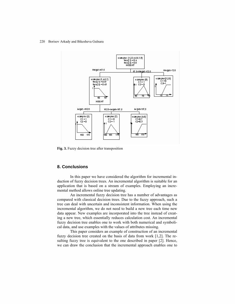
Fig. 3. Fuzzy decision tree after transposition

8. Conclusions

In this paper we have considered the algorithm for incremental in-duction of fuzzy decision trees. An incremental algorithm is suitable for an application that is based on a stream of examples. Employing an incre-mental method allows online tree updating.

An incremental fuzzy decision tree has a number of advantages as compared with classical decision trees. Due to the fuzzy approach, such a tree can deal with uncertain and inconsistent information. When using the incremental algorithm, we do not need to build a new tree each time new data appear. New examples are incorporated into the tree instead of creat-ing a new tree, which essentially reduces calculation cost. An incremental fuzzy decision tree enables one to work with both numerical and symboli-cal data, and use examples with the values of attributes missing.

This paper considers an example of construction of an incremental fuzzy decision tree created on the basis of data from work [1,2]. The re-sulting fuzzy tree is equivalent to the one described in paper [2]. Hence, we can draw the conclusion that the incremental approach enables one to


obtain a decision tree of the same quality as if it were built from scratch. Further research will be devoted to the possibility of using the incremental approach in constructing other kinds of fuzzy decision trees described in [6].

9. References

1. J. Zeidler, Michael Schlosser. Fuzzy Handling of Continuous-Valued Attributes in Decision Trees // In: Proc. ECML-95 Mlnet Familiarization Workshop "Statistics, Machine Learning and Knowledge Discovery in Da-tabases", Heraklion, Crete, Greece, April 28-29, 1995, 41-46.

2. J. Zeidler, Michael Schlosser. Continuous-Valued Attributes in Deci-sion Trees // In: Information Processing and Management of Uncertainty in Knowledge-Based Systems (IPMU'96), Granada, Spain, 1-5 July 1996, Proceedings, Volume I, S. 395-400.

3. Utgoff P. E., Berkmann N. C., Clouse J. A. Decision Tree Induction Based on Efficient Tree Restructuring // In: Machine Learning, 29, 1997, pp. 5-44.

4. Utgoff P. E. Incremental induction of decision trees // In: Machine Learning 4, 1989, p. 161-186.

5. Utgoff P.E. An improved algorithm for incremental induction of de-cision trees // In: Machine Learning: Proceedings of the Eleventh Interna-tional Conference, 1994, p. 318-325.

6. Bikesheva G., Borisov A. Fuzzy Decision Trees: Methods and Prob-lems // In: Proceedings of Riga Technical University, Information technol-ogy and management science, Riga 2002, Vol. 5, Issue 10, pp. 10-19.

7. Zadeh L. A. Fuzzy sets // In: Information and Control, 8, 1965, p. 407-428.

8. Borisov A., Alexeyev A. et al. Fuzzy Information Processing in Deci-sion Making Systems, Moscow, Radio i Sviaz Publishers, 1989 (In Rus-sian).

9. Wang Xizhao and Jiarong Hong. On the handling of fuzziness for continuous-valued attributes in decision tree generation. Fuzzy Sets and Systems, 99 (1998), p.283-290.

10.Yufei Yuan and Michael J.Shaw. Induction of fuzzy decision trees. Fuzzy Sets and Systems, 69 (1995), p.125-139.

11. Kosko, B. Fuzzy Engineering, Prentice Hall, Inc. 1997. 12. Quinlan, J.R. C4.5:Programs for Machine Learning. Morgan

Kauffman.1993.


Fuzzy Binary Tree Model for European-Style Vanilla OptionsSilvia MuzzioliDepartment of Economics, University of Modena and Reggio Emilia,[email protected] ReynaertsDepartment of Applied Mathematics and Computer Science, GhentUniversity, [email protected]

Abstract The derivation of the risk neutral probabilities in a bi-nary tree, in the presence of uncertainty on the underlying asset moves,boils down to the solution of dual fuzzy linear systems. The issue haspreviously been adressed and different solutions to the dual systemshave been found. The aim of this paper is to apply a methodologywhich leads to a unique solution for the dual systems.

Keywords Dual fuzzy linear systems, vanilla option, binary tree.

1 Introduction

The plan of the paper is the following. In section 2 we recall the fi-nancial problem and we introduce the vector solution to dual fuzzylinear systems. In section 3 we highlight that the system, connectedto the financial problem, has no solution if one applies standard fuzzyarithmetic. In section 4 we propose the vector solution to that systemand in section 5 we show the algorithm in order to compute the vectorsolution. The last section concludes.

2 European-style plain vanilla options

A (European-style Plain Vanilla) option is a financial security thatprovides its holder, in exchange for the payment of a premium, theright but not the obligation to either buy (call option) or sell (putoption) a certain underlying asset at a certain date in the future for aprespecified price K. The binary tree model of Cox-Ross-Rubinstein(1979) can be considered as a discrete-time version of the Black &Scholes (1973) model. The following assumptions are made: (A1) the

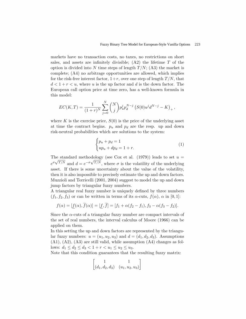
markets have no transaction costs, no taxes, no restrictions on shortsales, and assets are infinitely divisible; (A2) the lifetime T of theoption is divided into N time steps of length T/N ; (A3) the market iscomplete; (A4) no arbitrage opportunities are allowed, which impliesfor the risk-free interest factor, 1+r, over one step of length T/N , thatd < 1 + r < u, where u is the up factor and d is the down factor. TheEuropean call option price at time zero, has a well-known formula inthis model:

EC(K,T ) =1

(1 + r)N

N∑j=0

(N

j

)pjup

N−jd

(S(0)ujdN−j −K

)+,

where K is the exercise price, S(0) is the price of the underlying assetat time the contract begins. pu and pd are the resp. up and downrisk-neutral probabilities which are solutions to the system:

pu + pd = 1upu + dpd = 1 + r.

(1)

The standard methodology (see Cox et al. (1979)) leads to set u =eσ√T/N and d = e−σ

√T/N , where σ is the volatility of the underlying

asset. If there is some uncertainty about the value of the volatility,then it is also impossible to precisely estimate the up and down factors.Muzzioli and Torricelli (2001, 2004) suggest to model the up and downjump factors by triangular fuzzy numbers.A triangular real fuzzy number is uniquely defined by three numbers(f1, f2, f3) or can be written in terms of its α-cuts, f(α), α in [0, 1]:

f(α) = [f(α), f(α)] = [f, f ] = [f1 + α(f2 − f1), f3 − α(f3 − f2)].

Since the α-cuts of a triangular fuzzy number are compact intervals ofthe set of real numbers, the interval calculus of Moore (1966) can beapplied on them.In this setting the up and down factors are represented by the triangu-lar fuzzy numbers: u = (u1, u2, u3) and d = (d1, d2, d3). Assumptions(A1), (A2), (A3) are still valid, while assumption (A4) changes as fol-lows: d1 ≤ d2 ≤ d3 < 1 + r < u1 ≤ u2 ≤ u3.Note that this condition guarantees that the resulting fuzzy matrix:[

1 1(d1, d2, d3) (u1, u2, u3)

]

Fuzzy Binary Tree Model for European-Style Vanilla Options 223

has always full rank for all d ∈ (d1, d2, d3) and for all u ∈ (u1, u2, u3).There is no fuzziness in the risk free rate of interest, since it is givenat time zero.A fuzzy version of the two equations of the system (1) should now beintroduced. This can be done (for each equation) in two different ways,since for an arbitrary fuzzy number f there exists no fuzzy number gsuch that f + g = 0 and for all non-crisp fuzzy numbers f + (−f) 6= 0:

pu + pd = (1, 1, 1), pu = (1, 1, 1)− pd

respectively

upu + dpd = (1 + r, 1 + r, 1 + r) upu = (1 + r, 1 + r, 1 + r)− dpd

where pu, pu = ((pu)1, (pu)2, (pu)3), and pd, pd = ((pd)1, (pd)2, (pd)3),are the fuzzy up and down probabilities.Therefore the linear system (1) can be rewritten in four different ways:

pu + pd = 1upu + dpd = 1 + r

pu = 1− pdupu + dpd = 1 + r

pu = 1− pddpd = (1 + r)− upu

pu + pd = 1dpd = (1 + r)− upu

Those systems are called dual linear systems in the terminology ofMing Ma, et al. (2000). Buckley et al. (1991, 2002) propose thefollowing procedure to solve the fuzzy matrix equation Ax = b, wherethe elements, aij , of the n × n-matrix A and the elements, bi, of then×1-vector b are triangular fuzzy numbers: (1) solve the linear systemby using fuzzy number arithmetic; (2) if no such solution exists usethe vector solution XJ , withXJ(α) = x | Aαx = bα, (Aα)ij ∈ aij(α), (bα)i ∈ bi(α).Muzzioli and Reynaerts (2004) prove that the same procedure can beapplied to dual fuzzy linear systems A1x + b1 = A2x + b2, where theelements of the n × n-matrices A1 and A2 and the elements of then × 1-matrices b1 and b2 are fuzzy numbers. Indeed, the dual fuzzysystem A1x+ b1 = A2x+ b2 has a vector solution X∗J , with α-cuts

X∗J(α) = x | A1αx+ b1α = A2αx+ b2α, (A1α)ij ∈ a1,ij(α),(A2α)ij ∈ a2,ij(α), (b1α)i ∈ b1,i(α), (b2α)i ∈ b2,i(α),

224 Muzzioli Silvia and Reynaerts Huguette

if all matrices A1,0−A2,0 = [a01,ij−a0

2,ij ], with a1,ij ∈ a1,ij(0) and a2,ij ∈a2,ij(0), are nonsingular. They also prove that the linear systems Ax =b and A1x+b1 = A2x+b2 have the same vector solutions if A = A1−A2

and b = b2 − b1.

3 Solution using fuzzy arithmetic

As we already mentioned, the first step when solving fuzzy linear sys-tems, is to use fuzzy arithmetic. Therefore the systems are expressedin α-cuts. This method is applied for each system, keeping in mindthat the coefficients as well as the unknowns are positive:System 1:

[pu, pu] + [pd, pd] = [1, 1]

[u, u][pu, pu] + [d, d][pd, pd] = [1 + r, 1 + r].

leads to the following solution :

pu =(1 + r)− du− d

pu =(1 + r)− du− d

pd =u− (1 + r)u− d

pd =u− (1 + r)u− d

.

Clearly, pu < pu. The conclusion is that the system has no solution inthe set of the fuzzy numbers if one applies fuzzy arithmetic. Note thatif one poses pu1 = pu and pu

1 = pu, one obtains the solution given inMuzzioli and Torricelli (2001) and (2004), i.e.:

p1u = [

(1 + r)− du− d

,(1 + r)− du− d

] p1d = [

u− (1 + r)u− d

,u− (1 + r)u− d

].

System 2:

[pd, pd] = [1, 1]− [pu, pu]

[u, u][pu, pu] + [d, d][pd, pd] = [1 + r, 1 + r].

leads to the solution proposed by Reynaerts and Vanmaele (2003):

pu =(1 + r)(u+ d)− d(d+ u)

uu− ddpd = 1− pu

pu =(1 + r)(u+ d)− d(d+ u)

uu− ddpd = 1− pu,


which is different from what was found for System 1. One can showthat pu < pu (and thus pd < pd). The conclusion is that the systemhas no solution in the set of the fuzzy numbers if one applies fuzzyarithmetic.System 3:

[pd, pd] = [1, 1]− [pu, pu]

[d, d][pd, pd] = [1 + r, 1 + r]− [u, u][pu, pu].


pu =(1 + r)− du− d

pu =(1 + r)− du− d

pd = 1− pu pd = 1− pu.

Remark that, if one considers the solutions for α = 0 and α = 1, onecan conclude that (pu)2 < (pu)1. Thus the system has no solution inthe set of the fuzzy numbers if one applies fuzzy arithmetic.System 4:

[pd, pd] + [pu, pu] = [1, 1]

[d, d][pd, pd] = [1 + r, 1 + r]− [u, u][pu, pu].


pu =(1 + r)(u+ d)− d(d+ u)

uu− ddpd = 1− pu

pu =(1 + r)(u+ d)− d(u+ d)

uu− ddpd = 1− pu.

Depending on the values of u and d, pu < pu or pd < pd. Thus thesystem has no solution in the set of the fuzzy numbers if one appliesfuzzy arithmetic.In sum, none of the four dual fuzzy linear systems has a solution ifone applies fuzzy arithmetic. More details on the properties of thesolutions to the four systems can be found in Muzzioli (2004).

4 Vector solution

Since the four dual fuzzy linear systems have no solution if one appliesfuzzy arithmetic, we now investigate the vector solution. This solution


of all four dual linear systems is obtained by solving System 1:

(Aα)1,1 = (Aα)1,2 = (bα)1 = 1 (bα)2 = 1 + r

(Aα)2,1 = u1 + α(u2 − u1) + λ1(u3 − u1 − α(u3 − u1)), λ1 ∈ [0, 1](Aα)2,2 = d1 + α(d2 − d1) + λ2(d3 − d1 − α(d3 − d1)), λ2 ∈ [0, 1].

The vector solution is:

pu(α) =(1 + r)− (d1 + α(d2 − d1) + λ2(d3 − d1)(1− α))

frac

pd(α) =u1 + α(u2 − u1) + λ1(u3 − u1)(1− α)− (1 + r))

frac,

λ1, λ2 ∈ [0, 1],frac = u1 − d1 + α((u2 − u1)− (d2 − d1)) + (1− α)(λ1(u3 − u1)

−λ2(d3 − d1)).

The marginals are:

pu(α) = [1 + r − d3 + α(d3 − d2)

u3 − α(u3 − u2)− d3 + α(d3 − d2),

1 + r − d1 − α(d2 − d1)u1 + α(u2 − u1)− d1 − α(d2 − d1)

]

pd(α) = [u1 + α(u2 − u1)− (1 + r)

u1 + α(u2 − u1)− d1 − α(d2 − d1),

u3 − α(u3 − u2)− (1 + r)u3 − α(u3 − u2)− d3 + α(d3 − d2)

]

Note that this solution is the same solution found in Muzzioli andTorricelli (2001,2004).

5 An algorithmic solution of the fuzzy system

Muzzioli et al. (2004) proposes a practical algorithm that finds directlythe marginals for each unknown. Therefore one has to solve 2k systems,where k is the number of fuzzy parameters in the original fuzzy system.Each element of the extended coefficient matrix of those systems iseither the lower or the upper bound of the α-cut of the correspondingelement of the original fuzzy extended coefficient matrix. The finalsolution is investigated by taking the minimum and the maximum ofthe solutions found in each system for each unknown. This procedure


ensures that all possible solutions, consistent with the parameters ofthe system, are taken, but it does not guarantee that the solutionsare fuzzy numbers. Thus an ex-post check is needed to exclude thesolutions that are not fuzzy numbers. If xj(1) does not belong to[xj(0), xj(0)] for all j, then there is no solution to the system. If oneapplies this algorithm to the financial example, one should solve thefollowing systems:

pu + pd = 1upu + dpd = 1 + r.

pu + pd = 1upu + dpd = 1 + r.

pu + pd = 1upu + dpd = 1 + r.

pu + pd = 1upu + dpd = 1 + r.

The solutions to those systems are resp.:pu = (1+r)−d

u−dpd = u−(1+r)

u−d .

pu = (1+r)−d

u−dpd = u−(1+r)

u−d .

pu = (1+r)−du−d

pd = u−(1+r)

u−d .

pu = (1+r)−d

u−dpd = u−(1+r)

u−d .

The final solution is obtained by taking the minimum and maximumfor each unknown. Since pu(1) and pd(1) belong to the resp. solutionintervals, the vector of fuzzy numbers,(

[ (1+r)−du−d , (1+r)−d

u−d ] [u−(1+r)u−d , u−(1+r)

u−d ]),

is a solution to the system. Remark that one obtains the same solutionas the vector solution in section 4.

6 Conclusions

The derivation of the risk neutral probabilities in a lattice framework,in the presence of uncertainty on the underlying asset moves, boilsdown to the solution of a fuzzy linear system. In this paper we haveinvestigated the solution of such a system by using the methodologyproposed by Muzzioli and Reynaerts (2004). The solution, that isthe same solution found in Muzioli and Torricelli (2001, 2004), is heregiven in terms of vector solution. The properties of such a solutionhave been highlighted.


References

[1] Black F, Scholes M (1973) The Pricing of Options and CorporateLiabilities, Journal of Political Economy

[2] Buckley JJ, Eslami E, Feuring T (2002) Fuzzy mathematics ineconomics and engineering, Studies in Fuzziness and soft com-puting, Phisica Verlag

[3] Buckley JJ, Qu Y (1991) Solving systems of linear fuzzy equa-tions, Fuzzy sets and systems 43: 33-43

[4] Cox J, Ross S, Rubinstein S (1979) Option pricing, a simplifiedapproach, Journal of Financial Economics 7: 229-263

[5] Friedman M, Ming M, Kandel A (2000) Duality in fuzzy linearsystems, Fuzzy sets and systems 109: 55-58

[6] Moore RE (1979) Methods and applications of interval analysis,SIAM Studies in Applied Mathematics

[7] Muzzioli S, Torricelli C (2001) A multiperiod binomial model forpricing options in a vague world, Proceedings of the second Inter-national Symposium on Imprecise Probabilities and Their Appli-cations: 255-264

[8] Muzzioli S, Torricelli C (2004) A Multiperiod Binomial Model forPricing Options in a Vague World, Journal of Economic Dynamicsand Control, Special Issue on Financial Modelling 28: 861-887

[9] Muzzioli S (2003) A note on fuzzy linear systems, Discussion pa-per n. 447, Economics Department, University of Modena andReggio Emilia.

[10] Muzzioli S, Reynaets H (2004) Dual fuzzy linear systems, submit-ted to Fuzzy sets and systems

[11] Reynaerts H, Vanmaele M (2003), A sensitivity analysis for thepricing of European call options in a binary tree model, Proceed-ings of the third International Symposium on Imprecise Probabil-ities and Their Applications: 467-481


Tree-Structured Smooth TransitionRegression

Joel Correa da Rosa1, Alvaro Veiga2, Marcelo Medeiros3

1 Department of Statistics of Federal University of Parana, e-mail: [email protected] Department of Electrical Engineering of Catholic University of Rio de Janeiro

e-mail: [email protected] Department of Economics of Catholic University of Rio de Janeiro e-mail:[email protected]

Abstract Over the recent years, many nonlinear models have been pro-posed, both in classical econometrics, where multiple regime linear modelslike STR (Smooth Transition Regression) are receiving much attention, andin machine learning theory, including recursive partitioning methods likeregression trees, artificial neural networks (ANN) and nonparametric re-gression. In this work, we try to combine the advantages of two of thesemodels: STR and CART. From the STR model we inherited statistical in-ferential tools available to specify, test and to provide diagnostic checks.The CART methodology offers an easy interpretation of the final modelthrough a binary tree that can be stated as logical sentences. In this paperwe present the methodology of a tree structured regression with smoothsplits instead of the traditional CART partitioning of the explanatory vari-ables space. The performance of this new approach is compared to CARTone in a set of benchmark datasets.

1 Introduction

In recent years, much attention has been devoted to nonlinear modeling.Techniques such as artificial neural networks, nonparametric regression andrecursive partitioning methods are frequently used to approximate unknownfunctional forms. In spite of their success in various applications, severaltimes these approaches lack interpretability due to the complexity of thefinal model. Some cases in which the fitted model can be given a reason-able interpretation, there are no inferential procedures that guarantee thestatistical significance of the parameters.

Send offprint requests to: [email protected]

The proposal of the present paper is the construction of a nonlinearregression model that combines aspects of two well-known methodologies:Classification and Regression Trees (CART) discussed in [1] and the SmoothTransition Regression (STR) (see [3] and [2]) by taking advantages of theirmain capabilities. Our model inherits from CART the simplicity and in-terpretability of the tree-based models while the STR framework providestools for inference-based decisions.

The CART methodology represents a unification of all tree-based clas-sification and prediction methods that have been developed since a firstapproach presented by [4]. It transformed the regression tree models in animportant nonparametric alternative to the classical methods of regression.Since then, the attractiveness of this methodology has motivated many au-thors to create hybrid modeling strategies that merge tree techniques withknown statistical methods.

This paper presents in Section 2 the basis of the proposal of a fuzzyregression tree called Tree-STR which can be found by applying sequentialtests of hypotheses. Section 3 brings an application of Tree-STR model tothe famous Boston Housing dataset. In Section 4, we compare our approachto CART one in a set of benchmark datasets by using in-sample and out-of-sample evaluation criteria. Finally, conclusions are presented in Section5.

2 Tree-STR model a new approach

Given a set of observations taken from the pair (yt,xt) in which y is aunivariate response variable and x is a vector of p explanatory variables,traditional regression techniques will try to explain the relationship betweenthem by assuming that errors follow a probability distribution.

A regression tree is often used as a nonparametric model which looks forthe best local prediction, or explanation, of a continuous response throughthe recursive partitioning of the predictor variables’ space.The fitted modelis usually displayed in a graph which has the format of a binary decision treewhich grows from the root node to the terminal nodes, also called leaves.

The idea proposed here is the simple substitution of CART sharp splitsby smooth splits in an operation that exchange step functions by continuoussmooth functions assuming values between 0 and 1. By doing this, the sim-plest tree model, which contains 2 terminal nodes, could be mathematicallywritten as:

yt = β1G1(xt; Ψ0) + β2G2(xt; Ψ0) + εt (1)

where G2(.) = 1 − G1(.).Assuming that the error term follows a probability distribution, we can

interpret the STR model in equation (1) as a simple regression tree in whichthe nodes contain fuzzy sets instead of binary partition of the dataset. Here,the commonest choice for function G(.) is the logistic function:

Tree-Structured Smo oth Transition Regression 231

G1(xt; Ψ0) =e−γ0(xs0t−c0)

1 + e−γ0(xs0t−c0)(2)

in which the vector Ψ0, associated to the partition of the root node(node 0), has three parameters γ0, c0 and s0. The first one takes account ofthe smoothness of the transition function while the second would representthe CART threshold. If the split is smooth, c0, the location parameter,indicates the value which the observations have equal membership degreesto the created nodes1. The parameter s0 indicates the index of the splittingvariable selected among the elements of the vector xt = (x1, x2, . . . , xp).As long as γ0 approaches infinity, the CART simplest tree is nested by theTree-STR model in (1).

The parameters β1 and β2 represent constant models to be fitted withinthe two terminal nodes.

A More complex tree model would correspond to a re-specification of(1) by splitting one of the two created nodes. If the first (node 1) is to besplit, the model equation, by omitting the argument of transition functions,is updated to:

yt = [β3G3(.) + β4G4(.)]G1(.) + β2G2(.) + εt (3)

where G4(.) = 1 − G3(.).The regression tree behind the model in equation (3) has 3 terminal

nodes that contain fuzzy sets with membership functions G1(.)G3(.), G1(.)G4(.)and G2(.).

2.1 Tree Growing Methodology

We adopt an inferential approach to grow the tree based on linearity testsof the kind proposed in [5]. In this framework, the Taylor expansion of thelogistic functions creates an auxiliary regression that could be used to testthe significance of splitting a node.

A problem that emerges from this procedure is the control of the overallerror in this sequence of tests. Here, we adopt a strategy that reduces thesignificance level whenever the tree grows. By forcing the size of the testto be lowered during the tree construction, we also avoid the use of post-pruning techniques.

The tree growing strategy is based on the modelling cycle in [6]. Thefinal decision for splitting a node will be taken after following the stepslisted below:

Step 1 Use the LM-type test to specify a node and a splitting variable.Step 2 Estimate model parameters by nonlinear least squares.Step 3 Conditionally on the nonlinear parameters, evaluate the significance

of the constants within the nodes.

1 The created nodes are labeled as node 1 and node 2

232 Correa da Rosa Joel, Veiga Alvaro, Medeiros Marcelo

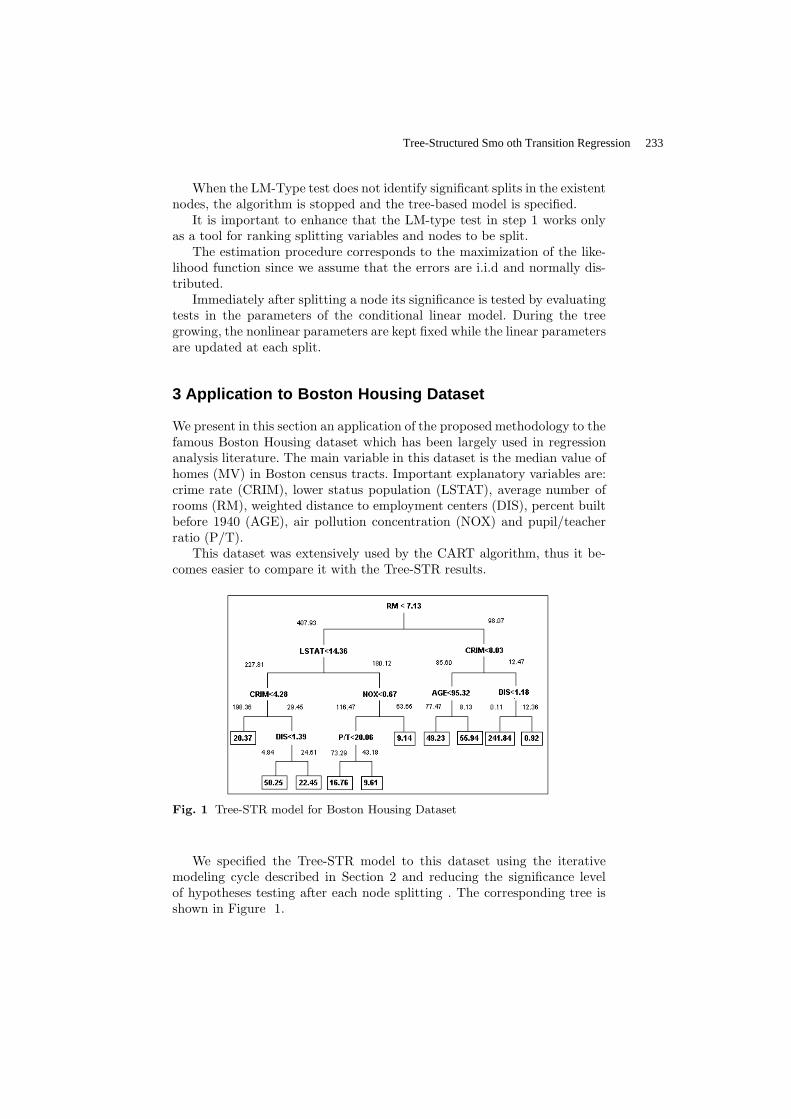
When the LM-Type test does not identify significant splits in the existentnodes, the algorithm is stopped and the tree-based model is specified.

It is important to enhance that the LM-type test in step 1 works onlyas a tool for ranking splitting variables and nodes to be split.

The estimation procedure corresponds to the maximization of the like-lihood function since we assume that the errors are i.i.d and normally dis-tributed.

Immediately after splitting a node its significance is tested by evaluatingtests in the parameters of the conditional linear model. During the treegrowing, the nonlinear parameters are kept fixed while the linear parametersare updated at each split.

3 Application to Boston Housing Dataset

We present in this section an application of the proposed methodology to thefamous Boston Housing dataset which has been largely used in regressionanalysis literature. The main variable in this dataset is the median value ofhomes (MV) in Boston census tracts. Important explanatory variables are:crime rate (CRIM), lower status population (LSTAT), average number ofrooms (RM), weighted distance to employment centers (DIS), percent builtbefore 1940 (AGE), air pollution concentration (NOX) and pupil/teacherratio (P/T).

This dataset was extensively used by the CART algorithm, thus it be-comes easier to compare it with the Tree-STR results.

Fig. 1 Tree-STR model for Boston Housing Dataset

We specified the Tree-STR model to this dataset using the iterativemodeling cycle described in Section 2 and reducing the significance levelof hypotheses testing after each node splitting . The corresponding tree isshown in Figure 1.


Some aspects illustrated in Figure 1 are quite different from the tradi-tional CART regression tree. First, instead of distributing the sample overthe terminal nodes, from this methodology we distribute the membershipdegree of a observation over them. Second, besides the threshold (location)parameters we also estimate a set of smoothness parameters that are notpresent in Figure 1 but which are shown in Table 1.

Table 1 Parameters Estimates of Logistic Functions in the Tree-STR Modelfitted to Boston Housing Dataset

Nonlinear Parameters

Location Smoothness

c0 = 7.13(0.003) γ0 = 1.62c1 = 14.36(1.166) γ1 = 1.93c2 = 8.03(1.085) γ2 = 3.53c3 = 4.28(1.086) γ3 = 65.13c4 = 0.67(4×10−4) γ4 = 10.63c5 = 95.32(4.317) γ5 = 115.36c6 = 1.18(0.001) γ6 = 103.41c9 = 20.06(5×10−4) γ8 = 245.24c8 = 1.39(0.145) γ9 = 5.04

(.) - s.e of estimates

In the Table 1, the parameters indexes, represent the location of thenode in the tree display. Thus, c0 is the location parameter at the root node(node 0).

Another difference from CART that should be outstanding is that theTree-STR model can fit a constant to the node that does not belong to therange of the observed responses. In fact, the predicted value, unlike CART,is obtained from a weighted sum of the constants within the nodes in whichthe weights are given by the membership of that observation to a terminalnode.

The sum of membership degrees within the terminal node is an impor-tant statistic to detect outliers candidates. A good example can be takenfrom Figure 1 where the lowest value (0.11) for this statistic is associatedto node 10 that would contain an unlikely prediction rule which is stated inFigure 2.

With the use of the function treefit present in the MATLAB statisticaltoolbox, the tree grown by the CART algorithm for this data obtainedinitially 95 terminal nodes. By following the same post-pruning principle,we found 30 terminal nodes with the Tree-STR model. After re-evaluatingthe tree performance by 10-fold cross-validation to get honest estimates ofthe errors, the estimated proportion of variance explained by CART was


If

Condition1 Number of Rooms greater than 7.13 and

2 Crime Rate greater than 8.03 and

3 Distance to employment center lower than 1.18Then

Predicted Value is 241.84

Fig. 2 Prediction Rule for Observations in Node 10

about 78 % and applying the same procedure to the Tree-STR model, thisproportion raised to 85 %.

0 5 10 15 20 25 300

10

20

30

40

50

60

70

80

90

Number of Leaves

MS

E

Cross−validation

Resubstitution

Fig. 3 Resubstitution and Cross-validation Estimates of Mean Square Error -Boston Housing Dataset

For the so-called resubstitution estimate, which means in-sample evalu-ation, the errors behaved quite differently in our model when compared toCART. We can see in Figure 3 that for small trees, the in-sample evalua-tion overestimates the mean square error and after reaching the supposed”right-sized” tree it starts to underestimate it.

4 Tree-STR vs CART Using Benchmark Datasets

To get a better evaluation of the Tree-STR performance when compared toCART algorithm, we selected 3 benchmark datasets to apply both method-ologies. A brief description of them is given below.


1. CPUs - The CPUs data is present in [7]. The purpose of applying re-gression trees methodology to this dataset is to provide a model thatexplains the performance of 209 different types of CPUs by some hard-ware characteristics.

2. Cars - This data were taken from MASS library in R software and itdescribes the prices and other 25 variables of 93 new cars models for the1993 year in the United States.

3. Auto imports - This dataset was taken from Ward’s 1985 AutomotiveYearbook and consists of 195 prices of cars followed by some featuressuch as: fuel consumption, length, width, engine size, among others.The informations are similar to the previous dataset, but there are morecontinuous variables to be included in a regression model.

Table 2 brings general information about the models fitted by CARTand Tree-STR respectively.

Table 2 Features of CART and Tree-STR Models fitted to Different Datasets

CART Number of Nodes Splitting Variables

Boston 9 X6,X5,X8 and X13

CPUs 5 X2, X3 and X4

Cars 3 X4

Auto Imports 9 X3,X5, X6, X7 and X8

Tree-STR Number of Nodes Splitting Variables

Boston 10 X5,X6,X7,X8, X11 and X13

CPUs 4 X3 and X4

Cars 2 X4

Auto Imports 9 X3,X4,X5, X6, X8 and X11

In Table 2, it should be noted that the tree sizes produced by eachmethod are very close, but the Tree-STR model captures more informationas long as it selects a greater number of splitting variables.

To evaluate the results in-sample and out-of-sample, we present in Table3 the resubstitution and 10-fold cross-validation estimates for the meansquare error (MSE).

Table 3 reveals that Tree-STR model has a better in-sample and out-of-sample performance on average if the mean square error measures thegoodness-of-fit.

5 Conclusions

In this paper we present a new approach that provides an alternative non-linear model that can be applied to regression problems. This model canbe interpreted as a multiple regime smooth transition regression, a neuralnetwork or a fuzzy regression.


Table 3 In-Sample and Out-of-Sample Evaluation of CART and Tree-STR Mod-els in Benchmark Datasets

In-sample evaluation of MSE

Dataset CART Tree-STR(LM)

Boston 12.56 11.55CPUs 3024.84 1283.72Cars 35.53 33.93

Auto Imports 3.26 7.23

Out-of-sample evaluation of MSE

Dataset CART Tree-STR(LM)

Boston 22.85(4.07) 18.10(2.74)

CPUs 3772.91(969.08) 3672.12(1774.36)

Cars 60.34(18.38) 39.89(15.61)

Auto Imports 8.84(1.60) 10.77(1.58)

(.) - s.e. of MSE estimates in 10 samples.

Application of this model to benchmark datasets has shown that thefitted regression can be presented in the same fashion as CART, but withsome useful additional informations such as the membership degrees of theobservations to the terminal nodes and the possibility of predicting beyondthe range of the dependent variable.

The overall results indicated that Tree-STR model yields parsimonioustree-based models that outperform CART trees if using the same number ofnodes. Additionally, as shown in the Boston Housing application, the mem-bership degrees are tools to identify outliers and influential observations.

References

1. L. Breiman and J. H. Friedman and R. A. Olshen and C. J. Stone, Classification

and Regression Trees (Wadsworth Int. Group, New York 1984).2. D. van Dijk, T. Tersvirta and P. H. Franses, Econometric Reviews 21 (2002)

1-473. C. W. J. Granger and T. Tersvirta, Modelling Nonlinear Economic Relation-

ships (Oxford University Press, Oxford 1993).4. J. Morgan and J. Sonquist, Journal of the American Statistical Association

58, (1963) 415-434.5. P. Saikkonen and R. Luukkonen, Scandinavian Journal of Statistics 15, (1988)

55-68.6. T. Tersvirta, Kybernetika 30, (1994) 319-330.7. B. D. Ripley, W. N. Venables Modern Applied Statistics with S-Plus(Springer

Verlag, New York 2002).


Discrete Dynamic Programming With Outcomes In Fuzzy Ordered Structures

Tadeusz Trzaskalik1, Sebastian Sitarz2

1Department of Operations Research, The University of Economics, ul. Bogucicka 14, 40-226 Katowice, Poland, [email protected]

2Institute of Mathematics, The University of Silesia, ul. Bankowa 14, 40-007 Katowice, Poland, [email protected]

Abstract. One way of generalization single criterion dynamic programming model is to consider partially ordered criteria structure. Generalization of Bell-man’s principle of optimality is employed to create solution of such problem. Or-dered structures defined by fuzzy numbers and triangular norms are considered. Numerical illustration is given at the and of the p aper. Keywords. discrete dynamic programming, fuzzy numbers, triangular norms.

1. Introduction

Decision problems with conflicting objectives and multiple stages can be considered as multi-objective dynamic programming problems. A survey has been presented by Li and Haimes (1989), more recently by Trzaskalik (1998). Another way of generalization single-criterion dynamic program-ming models is to consider outcomes in partially ordered criteria set. Mit-ten (1974) described a method for solving a variety of multistage decisions in which the real value objective function is replaced by preference rela-tion. Sobel (1975) extended Mitten’s result to infinitive horizon for deter-ministic and stochastic problems. Preference order dynamic programming was described by Steinberg and Parks (1979). Henig (1985) defined a gen-eral sequential model with returns in partially ordered set. It is shown that Bellman’s principle of optimality (Bellman(1957)) is valid with respect to maximal returns and leads to an algorithm to approximate these returns. Discrete dynamic programming with partially ordered criteria set was also considered by Trzaskalik and Sitarz (2002).

Application of fuzzy logic to control started with the work written by Bellman and Zadeh (1970). Many contemporary approaches in this field are presented in Kacprzyk (1997).

The aim of the paper is to describe finite discrete model and solving procedure and partially ordered fuzzy structures. In Section 2 discrete dy-namic decision process is defined and solving procedure is described. In Section 3 two fuzzy ordered structures: one based on trapezoid fuzzy num-bers and the second – on triangular norm are considered. Two illustrative examples are given ins Section 4.

2. Dynamic programming in partially ordered structure

Discrete dynamic process P which consists of T periods is considered. Let us assume that for t=1,…,T, that: Yt is the set of all feasible state variables at the beginning of period t, YT+1 is the set of all states at the end of the process, Xt(yt) is the set of all feasible decision variables for period t and state yt∈Yt. We assume that all above sets are finite. Now let us define: Dt = dt = (yt , xt): yt∈Yt, xt∈Xt(yt) - the set of all period realizations in pe-riod t, Ω t: Dt →Yt+1 - transformations.

Process P is given if sets Y1, …,YT+1, X1(y1),…XT(yT) and transforma-tions Ω 1 , …,ΩT are identified.

Let us denote

D = d=(d1,…,dT): ∀t∈1,…,T yt+1=Ω t(yt, xt) and xT∈XT(yT) - the set of all process realizations.

Dt(yt) =(yt, xt): xt∈Xt(yt) - the set of all realizations in period t which begin at yt.

d(yt) = (yt xt,…, yT,xT) - the backward partial realization which begins at yt.

D(yt) =d(yt): d∈D - the set of all backward partial realizations, which begin at yt.

D(Yt) =D(yt): yt∈Yt - the set of all backward partial realizations for Yt. d’(yt) = (y1, x1,…, yt-1, xt-1) - the forward partial realization which ends

at yt=Ω t(yt-1, xt-1).

Discrete Dynamic Programming With Outcomes In Fuzzy Ordered Structures 239

D’(yt) =d’(yt): d∈D - the set of all forward partial realizations, which end at yt.

D’(Yt) =D’(yt): yt∈Yt - the set of all forward partial realizations for Yt. (W, ≤, ) - ordered structure with binary relation ≤ and binary operator

fulfilling following conditions: ∀a∈W a≤a,

∀a,b∈W a≤b ∧ b≤a ⇒ a=b, ∀a,b,c∈W a≤b ∧ b≤c ⇒ a=c,

∀a,b,c∈W a(bc) = (ab)c, ∀a,b,c∈W a≤b ⇒ ac≤bc ∧ ca≤cb.

Relation < is defined as follows:

a<b ⇔ a≤b ∧ a≠b. Applying relation ≤ we define for each finite subset A⊂W the set of

maximal elements: max(A) = a*∈A: ~∃ a∈A a* < a.

For t=1,…,T let (W, ≤, t) be a sequence of ordered structures and ft:Dt→W a sequence of period criteria functions. Applying period criteria functions f t, we define functions Ft :D(Yt)→W in the following way:

FT = fT

Ft = ft t (f t+1 t+1 (…(fT-1 T-1 fT))), t=T-1,…,1.

Let F: D→W be the function defined in one of the following ways: i) F=F1 ii) F=GT

F is called the multi-period criteria function. Discrete dynamic decision process (P, F) is given if there are defined: discrete dynamic process P and multi-period criteria function F.

Realization d*∈D is efficient, iff

F(d*) ∈ max F(D). Our problem is to find the set of all maximal values of the process i.e.

set max F(D). Theorem 1. Decision dynamic process (P, F) is given. For all t=T-

1,…,1 and all yt∈Yt holds: a) max Ft(D(yt) = max f t(dt) t max(Ft+1(d(Ω t(dt))): dt∈Dt(yt). b) maxF(D) = max maxF1(d(y1)): y1 ∈Y1.

240 Trzaskalik Tadeusz and Sitarz Sebastian

Proof. Trzaskalik and Sitarz (2000), (Theorem 2, Theorem 3, p. 191). Theorem 1 yields backward iterative computational method.

Step 1. Compute maxFT(D(yT) for all states yT∈YT. Step t (for t=T-1, …, 1). Compute maxFt(D(yt) for all states yt∈Yt by using theorem 1a). Step T. Compute maxF(D) by using theorem 1b).

3. Fuzzy ordered structures

3.1. Fuzzy numbers

We consider trapezoidal fuzzy numbers with membership function:

( )

0, , <n+ ,

1, ,

1 , ( , )

1 , ( , )

x m

x m nm xx x m m

x nx n n

α β

µ αα

ββ

∈<−∞ − > ∪ ∞ > ∈< > −= − ∈ − −

− ∈ +

Shortly we denote such trapezoidal numbers as (m, n, α , β), and the set of all trapezoidal fuzzy numbers as Tm,n, α,β. We use fuzzy max-order (Furu-kava (1994))

A≤F B ⇔ ∀α∈[0, 1] (sup Aα≤sup Bα) ∧ (inf Aα≤ inf Bα) where Aα=x∈: µA(x)≥α, Bα= x∈: µB(x)≥α are α-cuts of fuzzy numbers A, B.

This relation in a class of trapezoidal fuzzy numbers has the following form:

(m1, n1, α1, β1) ≤F (m2, n2, α2, β2) ⇔ (m1-α1≤m2-α2) ∧ (m1≤m2) ∧ (n1≤n2) ∧ (n1-β1≤n2+β2),

We add fuzzy numbers by adding parameters:

(m1, n1, α1, β1) + (m2, n2, α2, β2) ⇔ (m1+m2, n1+n2, α1+n2, β1+β2)


One can easily prove that triple (Tm,n,α,β, ≤F, +) is ordered structure. We

can built another ordered structure of fuzzy numbers using L-fuzzy num-bers presented by Furukava (1994).

3.2. Triangular norms

Let us consider following structure (W, ≤, ) consisting of: W = [0, 1] (real numbers between 0 and 1), ≤ (standard relation of comparing real numbers), =T (T-norm).

This triple creates ordered structures because every t-norm fulfills con-ditions:

∀a,b,c∈[0,1] T(a,T(b,c) = T(T(ab),c)

∀a,b,c∈[0,1] a≤b ⇒ T(a,c)≤T(b,c) ∧ T(c,a)≤ T(c,b)

4. Numerical illustrations

We consider a dynamic process which consists of 4 periods [T=4], in which:

Yt=0,1, for t∈1, 2 ,3, 4 Xt(yt)=Yt+1 for t∈1, 2 ,3 and yt∈Yt.

Ω t(yt, xt)= xt for yt∈Yt and xt∈Xt(yt)

Two examples presented below are considered over the same dynamic process. The difference lays in the structures of outcomes. Fuzzy numbers are used in example 4.1, and triangular norms are used in example 4.2.

Example 4.1 (fuzzy numbers)

In the example we use special case of trapezoidal fuzzy numbers i.e. tri-angular fuzzy numbers. We denote them as (m, α, β), where m is the cen-ter and α, β are deviation parameters. The outcomes are described in or-dered structure: (Tm,α,β, ≤F, +). The values of period criteria functions are as follows

f1(1,1) = (2, 2, 2); f2(1,1) = (5, 3, 4); f3(1,1) = (6, 3, 2); f1(1,0) = (3, 2, 1); f2(1,0) = (6, 3, 2); f3(1,0) = (4, 2, 2); f1(0,1) = (6, 2, 2); f2(0,1) = (4, 2, 1); f3(0,1) = (4, 1, 3);


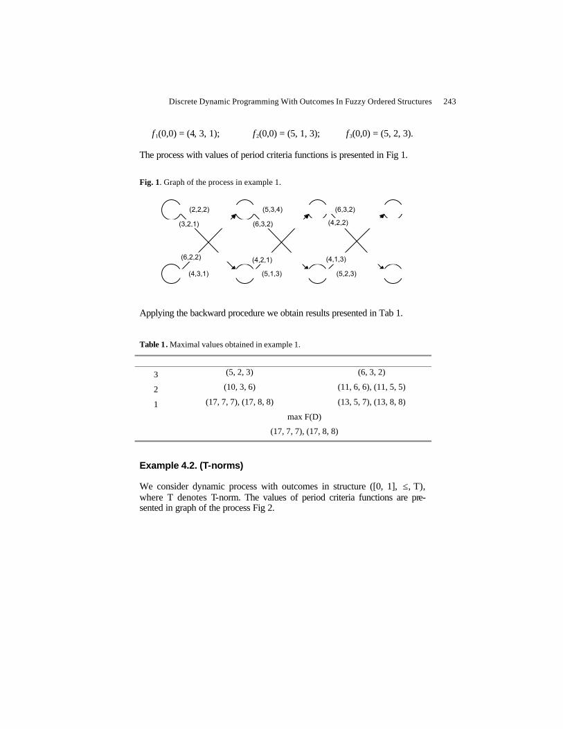
f1(0,0) = (4, 3, 1); f2(0,0) = (5, 1, 3); f3(0,0) = (5, 2, 3).

The process with values of period criteria functions is presented in Fig 1.

Fig. 1. Graph of the process in example 1.

1

0

1

0

1

0

1

0

(2,2,2)

(3,2,1)

(6,2,2)

(4,3,1) (5,1,3)

(4,2,1)

(6,3,2)

(5,3,4) (6,3,2)

(4,2,2)

(4,1,3)

(5,2,3)

Applying the backward procedure we obtain results presented in Tab 1.

Table 1. Maximal values obtained in example 1.

Example 4.2. (T-norms)

We consider dynamic process with outcomes in structure ([0, 1], ≤, T), where T denotes T-norm. The values of period criteria functions are pre-sented in graph of the process Fig 2.


3 (5, 2, 3) (6, 3, 2)

2 (10, 3, 6) (11, 6, 6), (11, 5, 5)

1 (17, 7, 7), (17, 8, 8) (13, 5, 7), (13, 8, 8)

max F(D) (17, 7, 7), (17, 8, 8)

Fig. 2. Graph of the process in example 2.

1

0

1

0

1

0

1

0

0.85

0.85

0.9

0.8 0.8

0.75

0.85

0.7 0.95

0.9

0.6

0.8

Applying the backward procedure we obtain results for chosen T- norms presented in Tab 2.

Table 2. Results obtained in example 2.

5. Conclusions

Dynamic programming model with outcomes in partially ordered criteria set gives a good possibility of modeling decision maker’s preference. Two examples of fuzzy structures were presented. The approach given in the paper can be easily extended and among dimensions defining criteria space real numbers, random variables, fuzzy numbers and other mathematical structures can be simultaneously considered.


min a, b) minimum 0.8 (0,1, 1,0, 0,0)

max a+b−1, 0 Lukasiewicz 0.55 (0,1, 1,0, 0,0), (1,0, 0,1, 1,1), (0,1, 1,1, 1,1)

ab probablistic 0.621 (0,1, 1,0, 0,0)

min , if max , 1

0 otherwise

a b a b =⎧⎨⎩

weak 0 (0,1, 1,0, 0,0), (1,0, 0,1, 1,1), (0,1, 1,1, 1,1)

References

Bellman, R.E. (1957) Dynamic Programming. Princeton University Press, Prince-ton, N.J.

Bellman, R.E., Zadeh, (1970) L.A. Decision making in fuzzy environment. Man-agement Science 17 141-164.

Furukava N. (1994) A parametric total order on fuzzy numbers and a fuzzy short-est route problem, Optimazation, 30 (1994) 367-377.

Henig, M.I. (1985) The principle of optimality in dynamic programming with re-turns in partially ordered sets”. Math. of Oper. Res., 10 3 462-470.

Li, D., Haimes, Y.Y. (1989) “Multiobjective dynamic programming: the state of the art”. Control Theory and Advanced Technology, 5 4 471-483.

Kacprzyk J. (1997) Multistage fuzzy control. A model-based approach to fuzzy control and decision making. Willey.

Mitten, L.G. (1974) “Preference order dynamic programming”. Management Sci-ence, 21 1 43-46.

Sobel, M.M.(1975): “Ordinal dynamic programming”. Management Science, 21, 9, 967-975.

Steinberg E., Parks, M.S. (1979) “A preference order dynamic program for a knapsack problem with stochastic reward”. Operational Research Society Journal 30 2 141-147.

Trzaskalik, T.: (1998) Multiobjective Analysis in Dynamic Environment, The Karol Adamiecki University of Economics in Katowice, 1998.

Trzaskalik, T., Sitarz, S. (2000) “Dynamic discrete programming with partially ordered criteria set”. In:Trzaskalik T., Michnik J. (eds.): Multiple objective and Goal Programming. Recent Developments. Physica-Verlag,186-195.


FUZZY MATHEMATICAL STRUCTURES AND GRAPH

THEORY

Plenary Report Fractal Methods of Graphs Partitioning

Kureichik V.V. and Kureichik V.M.

Fuzzy Mathematical Structures

A Method for Definingand Fuzzifying Mathematical Structures Ionin V.K. and Plesniewicz G.S. On Symmetric MV-Polynomials

Di Nola Antonio, Lettieri Ada and Belluce Peter Lattice Products, Bilattices and some Extensions of Negations, Triangular Norms

and Triangular Conorms Tarassov Valery B.

Soft Computing Methods in Graphs Theory and Applications

Definition of Optimum Allocation of the Service Centers Bershtein Leonid, Bozhenyuk Alexander and Rozenberg Igor

Evolutionary Algorithm of Minimization of Intersections and Flat Piling of the Graph Mathematic Models

Gladkov L.A. and Kureichik V.M. Use of a Fuzzy Strategy to Create the Shortest Hamiltonian Cycle

Piech Henryk and Ptak Aleksandra

Fractal Methods of Graphs Partitioning*

V.V.Kureichik, V.M.Kureichik

Taganrog State University of Radio Engineering

[email protected]; [email protected]

The problem of partitioning of the graph nodes on parts is considered.

For its decision genetic algorithms and fractals aggregation methods are of-

fered. It allows receiving partitioning with local optimum for polynomial

time. Complexity of algorithms has the square-law order on average.

Introduction

In 1980 B.Mandelbrot has specified on fractal geometry of natural systems (NS) [1,3]. Fractals are invariant to analyzed object and are capable to similar duplication at various existential levels and to the transfer of the information to system about infringement of stability of the structural condition. Fractals have properties of adaptation to external influence by reorganization of fractal sets (FS). For artificial systems the similarity of structures represents the determining property of FS and is realized only on the limited scales. According to [1-3,4,8] evolving systems have a fractal nature and a presence of directed not spontaneous selection and the self-coordinated evolution.

The new type of genetic algorithms of graphs partitioning on parts with minimization of total number of external edges is offered. These methods can be used in economics and finance. For example, when deciding the problem of optimal resources distribution, goods distribution between bases, shares distribution for shareholders etc. Strategy of partitioning is based on aggregation of fractals and the use of evolutions ideas [5]. Running time of algorithm (RTA) allows * Work is executed at financial support of the Russian Federal Property Fund (the

project 03-01-00336)

receiving local optimum. It roughly makes O (n2) - O (n3), where n – is a number of the graph nodes researched.

1. Problem statement. Fractal objects are similar, i.e. their kind does not undergo changes when changing scales. The sets having such structure are considered being ones possessing geometrical (scale) universality. Such sets of objects refer to fractal sets. Among these are Set of Cantor (SC) and Carpet of Serpinsky (CS) [1,2]. They possess a geometrical invariance and are called « sets of aver-age thirds ». At SC construction a piece of individual length [0,1] is divided into three equal parts and an average from them – an interval [1/3, 2/3] is cut out. Further the same happens to each piece. We re-ceive a sequence of pieces of the decreasing length. At the first stage it is one piece, on the second – two, on the third – 4, etc., on k-that – 2k. At k→∞ we have a set of points named SC. The total length of all cut out pieces is equal to 1. The circuit of a snowflake can be an example of a fractal object.

New strategy of the decision of the important combinatory problem of graph partitioning concerning to a class of NP-complete problems is proposed. In this paper, new and modified genetic algo-rithms (GA) with fractals aggregation for graph partitioning are of-fered. They differ by application of non-conventional architectures of genetic search (GS), and new genetic operators (GO) focused on use of knowledge of decided problems.

In [9-12] statement of the graph partitioning problem on the set or any number of parts is given. Cost function (CF) for a graph G partitioning will be written as follows:

∑ ∑= =

=n

i

n

jjiKK

1 1, ,

21 (i≠j), (1)

where Кi, j – is a number of connections between parts Вi and Вj at partitioning graph G on parts; l – is an amount of parts in partition-ing; K – is a total amount of edges at the graph partitioning. The standard problem of partitioning consists in minimization K (K→min).

It follows from the previously mentioned that the decision of a graph partitioning problem based on full search is inconvenient because of the process exponential complexity. Thereupon various

250 Kureichik V.V.and Kureichik V.M.

heuristics of the decision of the given problems are developed [9]. Some new heuristics using various incident methods recently have appeared. These are methods of evolution simulation, simulated an-nealing, fractals aggregation and their updatings. They are based on the analysis and search of alternative variants of decisions; however they differ on technology and principles of realization.

There is the mechanism of aggregation (DLА) describing fractals creation. According to DLА the certain version of fractals can be received during the disorder growth. For example, a cluster is given growing as follows: eventually the molecule joins it and sticks to it at once. This process is named aggregation. Let particles diffuse to growing cluster randomly. The aggregation of particles proceed-ing in conditions of random movement, it is DLА [5].

2. Fractal algorithm of the graph partitioning. Let us con-sider an algorithm of graph partitioning based on fractals aggrega-tion [1,5,9-12]. The mechanism of the graph partitioning is based on seven principles: • essential dependence on entry conditions; • "Razor Okkama"; • use of various evolution models; • clusters construction (the massifs of graph nodes definitely con-

nected among themselves); • clusters factorization, i.e. reduction of dimension the graph by

representation of clusters as the new incorporated nodes of the graph;

• DLA, i.e. the aggregation proceeding in conditions of random, di-rected and combined connection of the graph nodes to clusters;

• hierarchy. Such mechanism is open, i.e. the amount of used principles

can be varied. We shall describe this process in detail. Process of clusters creation is based on the mechanism of construction of the minimal files in the graph or hypergraph [10]. Let us introduce a concept of cluster in graph G = (X, U). Cluster is a part of graph Ф⊆G, and Ф = (Х1, U1), Х1⊆X, U1⊆U. Nodes of the cluster are con-nected by internal edges to other nodes Х\Х1 of graph G. Let us name the capacity of a subset of cluster external edges as f. We shall name cluster Фi as minimal one, if for any another cluster Фj, Фj ⊂Фi

Fractal Methods of Graphs Partitioning 251

the condition fi ≤ fj is satisfied. In other words, the removal of any nodes from Фi (Фi\Xm) results to new cluster with a big number of ex-ternal edges. By definition we shall consider:

(∀Фi ⊆G) (Фi≠∅), (∀xi ∈X) (xi – minimal cluster). (2)

It means that minimal cluster (CM) cannot be empty. Besides in a trivial special case each node of the graph forms CM. Construction of CM is connected to allocation of all subsets of set X, and it makes 2n, if |Х | = n. In this connection are developed heuristics of alloca-tion of a clusters set and CM. These heuristics are based on theorems of the minimal files in graphs [5].

Theorem 1. If Фi and Фj are CM and Фi ⊄ Фj ∧ Фj ⊄ Фi then

Фi∩Фj =∅. Theorem 2. Let Фi, Фj – CM. If Фs = Фi ∪ Фj ∧ fs <fi ∧ fs <fj

then Фs is CM. Theorem 3. Let Ф1, Ф2, …, ФL – the CM, and any associa-

tion of a part from them is not CM. If Фi = Ф1 ∪ Ф2 ∪…∪ ФL ∧ fi <f1

∧ fi <f2, …, ∧ fi <fL then Фi is CM. The proof of theorems 1,2,3 follows from the analysis of CM

construction. On the basis of these theorems we shall describe heu-ristic algorithm of CM construction. From the theorem 1 it follows that generally at full search procedure of CM construction is con-verging. The decision is unique at the graph partitioning when the number of nodes of partitioning is not set. At the graph partitioning on the set number of nodes the amount of decisions generally repre-sents some subset of alternatives. Theorems 2 and 3 allow aggregat-ing (uniting) clusters.

Let us present heuristic indistinct algorithm of CM construc-tion in the graph. 1. Let us order all local degrees of the graph nodes as trivial CM. 2. Starting by nodes with the greater local degree, we shall analyze

all nodes of graph G in pairs. If a pair of nodes (хi, хj) for which it is defined:

f =ρ(хi) +ρ(хj)-2ri, j, (3)

then Ф = (Х1, U1), Х1 = хi, хj and Ф is CM. Here ρ(хi), ρ(хj) –are local degrees of nodes хi, хj; ri, j – is a number of the edges con-necting nodes хi, хj among themselves, f –is a number of the edges


connecting CM with other nodes of graph G, and f < ρ(хi), f <ρ(хj). Minimal cluster Ф is put in the special list, and nodes хi, хj are ex-cluded from consideration. Transition to 2. If new CM was not formed, transition to 3.

3. We replace nodes хi, хj in CM by one node хi, j. Thus the edges connecting хi and хj, are removed, and edges from nodes хi, хj to other nodes are attributed to the common node хi, j. We have graph G '.

4. In graph G ' all nodes are analyzed. If there are three nodes ха, хв, хс for which the following is fair:

f =ρ(хa) +ρ(хв) +ρ(хc)-2ra, у-2rв, c-2ra, c, (5) and f <ρ(хa), f <ρ(хв), f <ρ(хc) the top хa, хв, хc forms CM accord-ing to the theorem 3. Transition to 2. Minimal cluster will be worn out in the list. If the CM is not present more, transition to 4.

5. Let's increase parameter of CM capacity by unit and we pass to 3. If CM capacity is equal to number of nodes of the set part of parti-tioning or it is equal to number of nodes of the graph, transition to 5.

6. The end of work of algorithm. The given algorithm can be applied for construction of the

set amount of the CM, the set capacity, and also it is used for con-struction of quasioptimal cluster, when fi-fj≤ε. Here ε - is the least relative deviation from capacity of CM (ε=0,1,2, …).

After construction of a set of CM if in graph G there were free nodes, it is necessary to carry out procedure of aggregation. It con-sists in a trial premise of nodes in CM with analysis of CF. The top is located in CM if its infringement occurs on the size which is not exceeding ε. If after the second step there were free nodes, proce-dures of joint evolution are realized.

Let us define labor input of the given algorithm. Let Np -be a size of a population, Ns – be an amount of the received descendants, NG – be an amount of GA generations. Then the common labor input of algorithm can be defined roughly:

Т ≈ tf [(Np tp + Ns ts + (Np + Ns) tc] NG, (4) where tf – is a labor input of minimal cluster construction; tp –

is a labor input of construction of one chromosome (the alternative decision) in a population (a set of decisions); ts – is a labor input of generation of one descendant; tc – is a cumulative labor input of se-


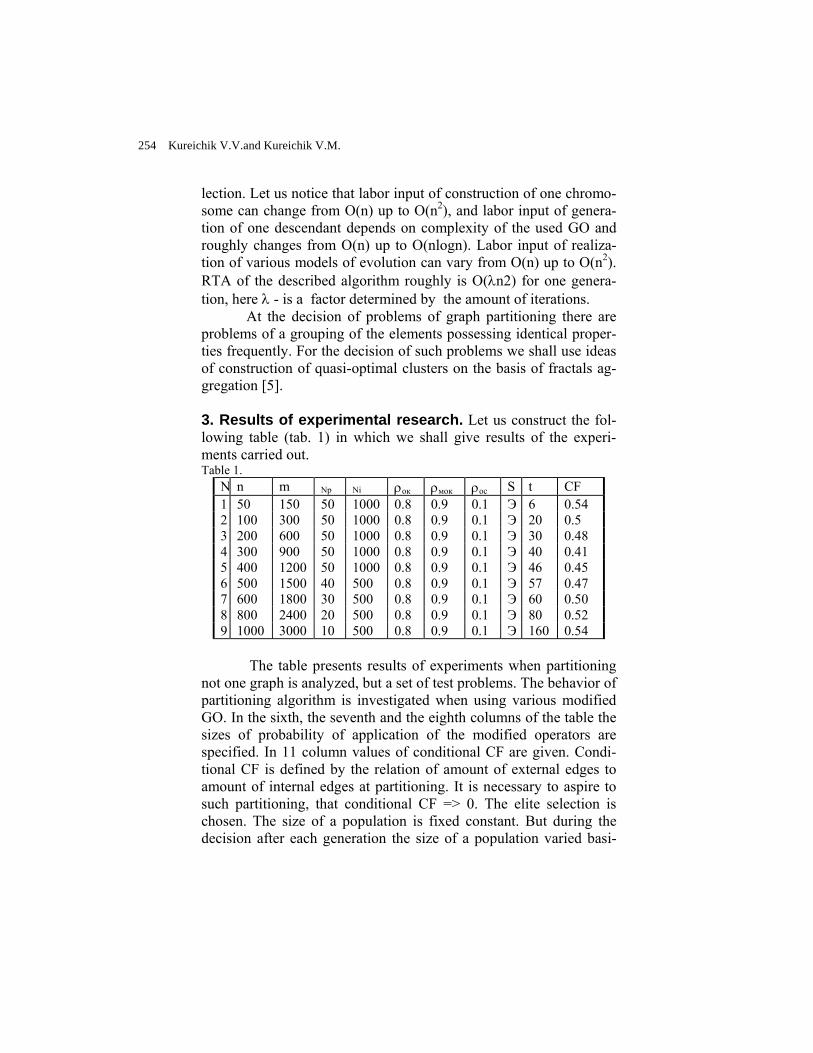
lection. Let us notice that labor input of construction of one chromo-some can change from O(n) up to O(n2), and labor input of genera-tion of one descendant depends on complexity of the used GO and roughly changes from O(n) up to O(nlogn). Labor input of realiza-tion of various models of evolution can vary from O(n) up to O(n2). RTA of the described algorithm roughly is O(λn2) for one genera-tion, here λ - is a factor determined by the amount of iterations.

At the decision of problems of graph partitioning there are problems of a grouping of the elements possessing identical proper-ties frequently. For the decision of such problems we shall use ideas of construction of quasi-optimal clusters on the basis of fractals ag-gregation [5]. 3. Results of experimental research. Let us construct the fol-lowing table (tab. 1) in which we shall give results of the experi-ments carried out. Table 1.

N n m Np Ni ρок ρмок ρос S t CF 1 50 150 50 1000 0.8 0.9 0.1 Э 6 0.54 2 100 300 50 1000 0.8 0.9 0.1 Э 20 0.5 3 200 600 50 1000 0.8 0.9 0.1 Э 30 0.48 4 300 900 50 1000 0.8 0.9 0.1 Э 40 0.41 5 400 1200 50 1000 0.8 0.9 0.1 Э 46 0.45 6 500 1500 40 500 0.8 0.9 0.1 Э 57 0.47 7 600 1800 30 500 0.8 0.9 0.1 Э 60 0.50 8 800 2400 20 500 0.8 0.9 0.1 Э 80 0.52 9 1000 3000 10 500 0.8 0.9 0.1 Э 160 0.54

The table presents results of experiments when partitioning

not one graph is analyzed, but a set of test problems. The behavior of partitioning algorithm is investigated when using various modified GO. In the sixth, the seventh and the eighth columns of the table the sizes of probability of application of the modified operators are specified. In 11 column values of conditional CF are given. Condi-tional CF is defined by the relation of amount of external edges to amount of internal edges at partitioning. It is necessary to aspire to such partitioning, that conditional CF => 0. The elite selection is chosen. The size of a population is fixed constant. But during the decision after each generation the size of a population varied basi-


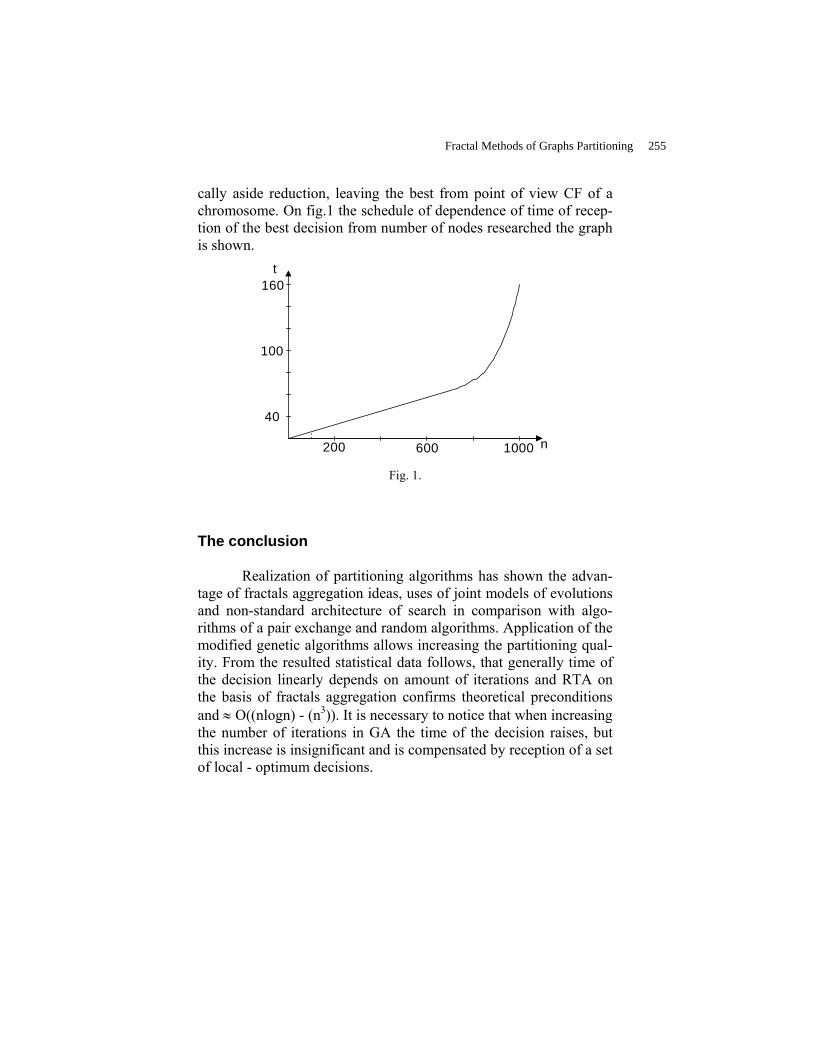
cally aside reduction, leaving the best from point of view CF of a chromosome. On fig.1 the schedule of dependence of time of recep-tion of the best decision from number of nodes researched the graph is shown.

200 600 1000

40

100

160

n

t

Fig. 1.

The conclusion

Realization of partitioning algorithms has shown the advan-tage of fractals aggregation ideas, uses of joint models of evolutions and non-standard architecture of search in comparison with algo-rithms of a pair exchange and random algorithms. Application of the modified genetic algorithms allows increasing the partitioning qual-ity. From the resulted statistical data follows, that generally time of the decision linearly depends on amount of iterations and RTA on the basis of fractals aggregation confirms theoretical preconditions and ≈ O((nlogn) - (n3)). It is necessary to notice that when increasing the number of iterations in GA the time of the decision raises, but this increase is insignificant and is compensated by reception of a set of local - optimum decisions.


References

1. Cronover R.M. Fractal and chaos in dynamic systems. Bases of the theory. M.: the Postmarket, 2000.

2. Pajtgen H.O., Rokhner P.H. Beauty of fractals. M.: the World, 1990

3. Prigozhin И., Stengers I. Order from chaos. M.: Progress, 1986. 4. Goldberg D.E. Genetic Algorithms in Search, Optimization and

Machine Learning. USA: Addison-Wesley Publishing Company, Inc., 1989.

5. Emeljanov V.V., Kureichik V.V., Kureichik V.M. Theory and practice of evolution simulation. – M.: Физматлит, 2003. – 432 p.

6. Kureichik V.V. Evolutionary, synergetic and homeostatic methods of decision-making. The monography. Taganrog: Publishing house TRTU, 2001.

7. Batishchev D.A. Genetic algorithms of the decision of extreme problems. Voronezh: Publishing house VGTU, 1995.

8. Kureichik V.M. Genetic algorithms: the Monography. Taganrog: Publishing house TRTU, 1998.

9. Sherwani N. Algorithms for VLSI Physical Design Automation, Kluwer Academic Publishers, Boston/Dordrecht/London, 1995.

10.Morozov K.K., Melihov A.N., Kurejchik V.M., etc. Methods of partitioning of circuits РЭА on structurally finished parts. M.: the Soviet radio, 1978.

11.Chandrasekharam R., Subhramanian and chadhurys. Genetic algorithms for node partitionaly problem and application in VLSI design // IEEE Proc-E, v.140, N.5, September, 1993.

12.Kureichik V.M., Kureichik V.V. Genetic algorithm of partitioning the graph // Izvestija of The Russian Academy of Science, 5, 1999.


A Method for Defining and Fuzzifying

Mathematical Structures

V.K.Ionin1 and G.S.Plesniewicz2

1 Moscow Power Institute (technical university) [email protected] ”MATI”-Russian University of Technology [email protected]

Abstract. A new method for defining mathematical structures and themethod for their fuzzifying is presented. In particular, the definition offuzzy vector space over arbitrary field is given.

1 Introduction

In [1,2] one of the authors (V.K.Ionin) has proposed some verygeneral method for defining mathematical structures. Briefly, themethod consists in the following.

Let K be any category, A,B be its objects, and Γ ⊆ Hom(A,B)be some set of morphisms from A to B. Given object X let (X, F, Φ)be such that (a) F ⊆ Hom(A,X), Φ ⊆ Hom(X,B); (b)ΦF⊆ Γ ; (c)it is not possible to extend F or Φ so that (a) is satisfied. (Here ΦFis the set of all compositions ϕf of morphisms ϕ ∈ Φ and f ∈ F .)

Remark. Due to the property (b), if F (or Φ) is known then Φ(or F , correspondingly) is uniquely defined.

We say that (X,F,Φ) is a Γ -space and (Φ,F ) is the Γ -structure.Thus, by mathematical structure we mean a Γ -structure. An objectXwith some Γ -structure can be considered as Γ -structure. One canconsider the set Γ as kind of the structure (F,Φ).

For example, consider one of the simplest mathematical structure- the structure of partial order. This structure is the pair (X,θ ) whereθ ⊆ X×X is a binary relation such that: (1) xθ x for all x ∈ X ; (2)if x θ y and yθ x then x = y for all x,y ∈ X ; (3) if x θ y and y θzthen x θ z for all x,y,z ∈ X.

It turns out that the structures of partial order can be representedas Γ -structures. Let A = B = 0, 1 and Γ be the set of all mappingfrom A to B besides the mapping Υ : Υ (0)=1, Υ (1)=0. For any Γ -space (X,F,Φ ) we define: xθ y if and only if ϕ(x) ≤ ϕ(y) for all

ϕ ∈ Φ. It is easy to prove that (X,θ ) is a partial order structure.Thus, we have the transition

(X, F, Φ) → (X, θ). (1.1)

On the contrary, let (X,θ ) be any partial order structure. Forany pair (a,b)∈ X×X we denote by fab the following mapping fromA to X as follows: fab(0) = a, f ab(1) = y. Then F =def fab|aθb.Defining Φ, we firstly denote by Φab the set of all mapping ϕ fromX to B such that if ϕ(a) = 1 then ϕ(b) = 1. Then, by definition,Φ is intersection of all Φab such that aθb.. Thus, we have the inversetransition

(X, θ) → (X,F, Φ). (1.2)

Both transitions (1.1) and (1.2) define the correspondence

(X,F, Φ) ↔ (X, θ) (1.3)

In this case we say that the Γ−structure (X,F,Φ ) is equivalentto the structure (X,θ ).

One goal of our investigations is in establishing correspondenceslike (1.3) between Γ -spaces and usual mathematical structures.

In the above definition of Γ -structure we implicitly suppose thatΓ is usual (i.e. crisp) subset of the set Hom(A,B). But if we re-place Γ by fuzzy subset of Hom(A,B) then we come to the conceptof fuzzy Γ -structure and fuzzy Γ−space. Thus, fuzzification of theconcepts related to crisp mathematical structures consists in apply-ing fuzzy sets of morphisms rather than crisp sets. ”Higher degree”of fuzzification is obtained when we consider Hom as fuzzy sets.

Remark. Our method is different from well known category the-ory method for specifying fuzzy structures (originating by J.Goguen).See for instance [3].

2 Preliminary Information

2.1 Γ -spaces

Let Γ be a subset of the set Hom(A,B) of all morphisms from Ato B where A and B are objects of a category K. A triple (X,F ,Φ)

258 Ionin V.K. and Plesniewicz G.S.

where X ∈ obK, is said to be the Γ -space if the following two axiomsare satisfied.

Axiom 1. For any F ′ ⊆ Hom(A,X) the following statementsare equivalent: (a) F ′ ⊆ F ; (b) ϕf ∈ Γ for any ϕ ∈ Φ and f ∈ F .

Axiom 2. For any Φ′ ⊆ Hom(X, B) the following statementsequivalent: (a) F ′ ⊆ F, (b) φf ∈ Γ for any ϕ ∈ Φ and f ∈ F ′ areequivalent: (c) Φ′ ⊆ Φ: (d) ϕf ∈ Γ for all ϕ ∈ Φ′ and f ∈ F .

It easy to note that these axioms are equivalent (together) to thefollowing two statements: (i) if f∈F, ϕ ∈ Φ then ϕf ∈ Γ , (ii) it isnot possible to extend sets F and Φ without loosing the statement(i).

If (X, F, ) is a Γ -space then we also say that X is the Γ -spacewith the Γ -structure (F,Φ )

2.2 Category K(Γ )

Let objects X,Y ∈ K are considered as Γ -spaces with Γ -structures(F,Φ ) and (G,Ψ ), correspondingly. Morphism h ∈ Hom(X,Y ) issaid to be Γ -morphism if ψhf ∈ Γ for any f ∈ F and ψ ∈ Ψ . It isclear that Γ -spaces and Γ -morphisms is a category.

2.3 Kind of structures

Denote by BijSet the category of sets and bijections and by BijKthe category of K’s objects and isomorphisms of K. Kind of struc-ture is a covariant functor T from BijK to BijSet. Elements ofT (X) are the structures of the object X. For example, the kind ofthe vector structure over an arbitrary field B is the covariant func-tor T : BijSet → BijSet which with every set X associates theset of pairs. Each pair contains in the first position a binary op-eration which specifies on X the structure of commutative group,and contains in the second position an operation - mapping fromB×X to X. The first operation responds to vector addition and thesecond one responds to multiplication of vectors by scalars. Usualidentities relates these operations. In section 3 we give an equiva-lent (though, strongly different in appearance) definition of kind ofthe vector structure. This allow us to give other definition of vectorspaces. (Similar situation arises with other kinds of structures.)

A Method for Defining and Fuzzifying Mathematical Structures 259

2.4 Fuzzy Γ -spaces

Now let Γ be a fuzzy subset of Hom(A, B), i.e. Γ is a mapping fromHom(A,B) to the segment of reals I = x | 0 ≤ x ≤ 1. Let us takesome function τ : I×I → I satisfying the following conditions:

τ(0,0) = 0, τ(1,1) = 1, τ(x,τ(y,z) = τ(τ(x,y),z) for all x,y,z∈ I.(Due associativeness of τ , it is convenient to write x τ y rather

than τ(x,y).)A triple (X,F,Φ) and a pair (F,Φ) are said to be the fuzzy Γ -

space and fuzzy Γ -structure for the object X ∈ ObK, if F and Φ arefuzzy subsets of Hom(A,X) and Hom(X,B), correspondingly, and thefollowing two axioms are satisfied.

Axiom 1˚ For any mapping F ′; Hom(A,X) → I the follow-ing two statements are equivalent: a) F ′(f) ≤ F (f) for all f ∈Hom(A,X); b) Φ(ϕ)τF ′(f) ≤ Γ (ϕf) for all f ∈ Hom(A, X) andϕ ∈ h=Hom(X,B).

Axiom 2˚ . For any mapping Φ’: Hom(X,B) → I the follow-ing two statements are equivalent: c) Φ’(ϕ) ≤ Φ(ϕ) for all ϕ ∈Hom(X,B); d) Φ′(ϕ)τF (f) ≤ Γ (ϕf) for all f ∈ Hom(A,X) andϕ ∈ Hom(X, B).

In the sequel for any Γ -space (X,F,Φ) we write (for brevity) γ, fand ϕ instead of Γ (γ), F (f) and Φ(ϕ), correspondingly.

2.5 Fuzzy sets of morphisns

We define fuzzy sets of morphisms as Hom(X, Y ) → I for anyΓ−spaces (X,F, Φ) and (Y,G, Ψ). The fuzzy set of morphisms de-pends on the function τ and on the fuzzy set Γ . In the sequel wewrite h instead of H(h). Suppose h the exact upper bound for λsuch that 0 ≤ λ ≤ 1, λτf ≤ h, ψτλ ≤ ψh for all f ∈ Hom(A.X) andψ ∈ Hom(Y, B).Let (X i, Fi, Φi), i = 1, 2, 3 be fuzzy Γ -spaces and h1 ∈ Hom(X1, X2),h2 ∈ Hom(X2, X3).

Lemma 1. If τ is a continuous function then the following in-equality holds:

h2τh1 ≤ h2h1. (2.1)

Remark. It is naturally to mean by a fuzzy subcategory of cat-egory K relative a function τ such mapping H of morphisms into


reals that enequality (2.1) is satisfied for any morphisms h1 andh2 having the composition h2nh1. Lemma 1 states that mapping Hdefines a fuzzy subcategory of the category of all Γ -spaces and allmorphisms for category K. It is clear that fuzzy subcategories arenatural generalizations of (crisp) subcategories.

3 Fuzzy Vector Spaces

In the sequel K is the category of all sets and all mapping, i.e. K= Set.

3.1 Connectivity and Separability

Let A,B ∈ ObK and Γ : Hom(A, B) → I. A fuzzy Γ -space (X,F,Φ)is said to be λ-connected (where λ ∈ I) if for any points p and q(possibly, p = q) there exists f ∈ Hom(A,X) that p,q ∈f(A) andf ≥ 1, If λ = 1 then (X, F, Φ) is said to be a strongly connectedfuzzy Γ -space. The space is to be λ-separable if for any differentpoints p and q there exists ϕ ∈ Hom(X,B) such that ϕ(p) 6= ϕ(q)and f ≥ 1. If λ = 1 then the space is to be strongly separable.

3.2 Lineear mapping

In the sequel B is any fixed field and A = B×B. A mapping Υ : A→ B is linear if there are a,b ∈ B that γ(x,y) = ax + by for all x,y∈ B. The set of all linear mapping from A to B is denoted by Λ.

3.3 Fuzzy vector space

Let Γ : Hom(A,B) → I be such that Λ = Γ−1(1) = γ|Γ (γ) = 1.Then Γ -space (X, F, Φ) is said to be a fuzzy vector Γ -space if thefollowing three axioms (besides axioms 1˚ and 2˚ ) are satisfied.

Axiom 3˚. X is not empty.Axiom 4˚. (X,F,Φ ) is strongly connected Γ -space.Axiom 5˚. (X,F,Φ) is strongly separable Γ -space.Let Γ ⊆ Hom(A,B), F ⊆ Hom(A,X), Φ ⊆ Hom(X,B) be in-

jections defined by equalities γ = 1, f = 1, ϕ = 1.The following two statements hold.


Lemma 3. A) If f ∈ F, ϕ ∈ Φ then ϕf ∈ Γ .B) If for a function f : A → X the condition ϕf ∈ Γ holds for

all ϕ ∈ Φ then f ∈ F.

3.4 Vector addition

In this section, members of X and B are called vectors and scalars,correspondingly.

By definition, a vector r is said to be a sum of vectors p andq (notation: r = p + q) if there are a function f ∈ F and scalarsx1, y1, x2, y2 such that

p = f(x1, y1), q = f(x 2, y2), r = f(x 1 + y1, x2 + y2).

Lemma 4. There is one and only one operation of vector additionsatisfying this definition.

3.5 Product of scalar and vector

By definition, a vector q is a product of a scalar λ and a vector p(notation: q = λ p) if there are scalars x, y and function f∈ F suchthat

p = f(x,y), q = f(λ x, λ y).

Lemma 5. There is one and only one operation of product ofscalars and vectors satisfying this definition.

4 Γ -Structures vs Bourbaki’s MathematicalStructures

A partial order structure (X,θ ) is an example of mathematical struc-ture according N.Bourbaki. In general, Bourbaki has given the fol-lowing definition. Let X be any set (so-called the support of thestructure) and τ j = τ j(X) (1 ≤ j ≤ n) are terms obtained by apply-ing usual set-theoretic operation (intersection, union, complement,Cartesian product, projects, and power set formation) starting X(considered as a variable). Then a mathematical structure is a tuple

(X, c1, c2, ..., cn) where cj ∈ τj(X) (1 ≤ j ≤ n) (4.1)


For example, if τ(X) = ℘(X × X) and θ ∈ ℘(X × X) then wehave the structure of binary relation. In particular, if we choose θto satisfy the conditions (1), (2) and (3) then (X,θ ) will be thestructure of partial order.

It is natural to consider term ℘(X×X ) as the kind of binaryrelation structure. But how to define naturally a kind of the structureof partial order?

It is clear that properties (1) ,(2) ,(3) can be represented by threeformulas:

∆ ⊆ θ, θ ∩ θ˚ ⊆ ∆, θθ ⊆ θ where ∆ is the ”diagonal” relation,θ˚ is the inverse relation, i.e.. θ˚ = (x,y) | (y,x) ∈ θ .

Then it is natural to consider the expression< ℘(X), (∆ ⊆ θ) & (θ ∩ θ˚ ⊆ ∆) & θθ ⊆ θ) >

as the kind of partial order relation. (This expression is an exampleof so-called statement of Tarskian algebra of binary relations.)

In general, let ω = ω(c1, c2, ..., cn) be a statement obtained fromvariable c1, c2, ..., cn by applying the set-theoretic operations, inclu-sion operation and propositional connectives. Then the expressionσ =< τ1, τ2, ..., τn > is the kind of the Bourbaki’s structure (4.1).

We propose the following conjecture. Let FinSet be the categorywhose objects are finite sets n = 0,1,2,...,n and morphisms aremapping n → m.

Conjecture. For each Bourbaki’s structure (4.1) with the kindσ there is an equivalent Γ -structure relatively category FinSet. Fur-thermore, there is an algorithm which returns Γ after applying to< σ, ω >.

We have verified the conjecture in particular cases when τ j (1≤j ≤ n) are all the same ℘(X×X) and operation ℘ is not used in ω.In other words, all cj(1 ≤ j ≤ n) are binary relations and ω is astatement of Tarskian algebra.

So, the conjecture is true for the case of the structures repre-sented by means of Tarski’s formalism for binary relations.

References

1. V.K.Ionin. Structures generated by sets of morphisms (in Rus-sian), Transactions of Sibirian Institute of Mathematics ”Researchin geometry and mathematical analysis”, Novosibirsk, 1987..


2. V.K.Ionin. Algebraic principles of building mathematical struc-tures, American Mathematical Society Translations, 1995, vol. 163(2).

3. L.A.Zadeh. Fuzzy sets , Information and Control. 1965, vol. 8(1).

4. S.E.Rodabaugh et al. (eds). Application of Category Theoryto Fuzzy Subsets, Kluwer Acad. Publishers, 1992.


On Symmetric MV - polynomials

Antonio Di Nola1 Ada Lettieri2 Peter Belluce 3

1 Introduction

An MV -algebra is an algebraic structure A = (A,⊕,∗ , 0) of type (2,1,0) satis-fying the following axioms:

(1) (x ⊕ y) ⊕ z = x ⊕ (y ⊕ z);

(2) x ⊕ y = y ⊕ x;

(3) x ⊕ 0 = x;

(4) (x∗)∗ = x;

(5) x ⊕ 0∗ = 0∗;

(6) (x∗ ⊕ y)∗ ⊕ y = (y∗ ⊕ x)∗ ⊕ x.

Therefore, if we define the costant 1 by 1 = 0∗ and the operation by x y =(x∗ ⊕ y∗)∗, then from (4), we obtain 1∗ = 0. Moreover, setting y = 1 in (6), itfollows x∗ ⊕ x = 1. On A two new operations ∨ and ∧ are defined as follows:x∨ y = (x∗ ⊕ y)∗⊕ y and x∧ y = (x∗ y)∗ y. The structure (A,∨,∧, 0, 1) is abounded distributive lattice. We shall write x ≤ y iff x ∧ y = x. A remarkableexample is the MV -algebra having, as support, the real interval [0, 1] and, asbasic MV -algebraic operations on [0, 1],

x ⊕ y = min (1, x + y);

x∗ = 1 − x.

We refer to this MV -algebra by [0, 1]. For each positive integer n, let Ln bethe set 0, 1

n, . . . , 1 endowed with the following operations :

x ⊕ y = min(x + y, 1),

1Dipartimento di Matematica e Informatica, Universita di Salerno, Via S. Allende, Baro-nissi (Salerno).e-mail: [email protected]

2Dipartimento di Costruzioni e Metodi Matematici in Architettura, Universita di NapoliFederico II, via Monteoliveto 3, 80134 Napoli, Italy.e-mail: [email protected]

3University of British Columbia, Dept. Math. , Vancouver,B.C. Canada

x∗ = 1 − x.

For each positive integer n, the algebra Ln is a finite totally ordered MV -algebra(MV -chain) and every non-trivial finite MV-chain is isomorphic to one of them.

Let A be an MV -algebra, x ∈ A and n a nonegative integer. In the sequelwe will denote by nx the element of A, inductively defined by 0x = 0, nx =(n − 1)x ⊕ x. Analogously we will set x0 = 1, xn = x xn−1. Moreoverwe consider the ∗ operation more binding than any other operation, and operation more binding than ⊕.

For all unexplained notions regarding MV -algebras we refer to [1] [2] [3] [4].Let L be the poset, under ⊆, of subalgebras of the MV-algebra [0, 1]. L then

has a unique minimal element, 0, 1, and a unique maximal element, [0, 1].L also contains atoms, that is subalgebras A ⊆ [0, 1] such that if A

′

⊆ A,then A

′

= 0, 1 or A′

= A. The algebra 0, 1/2, 1 is such an atom.Since, for a maximal ideal M of an MV-algebra A, A/M ∈ L, we have a

method to refine the structure of the maximal ideal space MaxA. Heuristically,smaller is the quotient A/M , larger is the maximal ideal M . In effect thisprovides a pre-order on the set of maximal ideals.

In this work we shall study these ideas for the set of maximal ideals of finitetype, that is maximal ideals M with A/M finite. We shall first look at supermaximal ideals M , that is, those maximal ideals M such that A/M is a smallas possible, namely A/M = 0, 1. Next we shall look at some classes of bigmaximal ideals M , that is, those maximal ideals M which if not super maximalare such that A/M is an atom of L.

Our study will use a class of MV-polynomials, that we will call symmetricwhich shall permit us to construct the appropriate MV-algebras.

The first part of this work concerns supermaximal ideals. In a booleanalgebra all maximal ideals are supermaximal (considering the boolean algebraas an MV-algebra).

Given an MV-algebra, its set of idempotents, B(A), is a subalgebra which is aboolean algebra. We shall examine extensions of B(A) in A, that is subalgebrasA′ of A such that B(A) ⊆ A′ ⊆ A, that have supermaximal ideals. We shallalso study properties of the set of supermaximal ideals.

The second part of this work will take up the case of certain extensions ofB(A) which may have big maximal ideals, and we shall study some propertiesof these algebras.

Both of these parts will be presented as a special case of subalgebras deter-mined by certain symmetric MV-polynomials.

Definition 1. Let A be an MV-algebra. An M ∈ MaxA is called of type n,provided that A/M ∼= Ln .

Definition 2. Let A be an MV-algebra. M ∈ MaxA is called of finite type, ifM is of type n for some integer n.

Definition 3. Given an MV-algebra A, an M ∈ MaxA is called supermaximal,in symbols SMax provided A/M ∼= 0, 1.

Definition 4. Given an MV-algebra A, we shall call M ∈ MaxA, big-maximaliff A/M ∼= S where S has not nontrivial MV -algebras.

266 Di Nola Antonio, Lettieri Ada and Belluce Peter

We shall focus on big-maximal ideals of finite type.Not every MV-algebra A has supermaximal ideals, for example [0, 1], or less

trivially, [0, 1]X . We shall construct algebras which do have super maximalideals, and some algebras where all maximal ideals are super maximal.

We shall look at the topological aspect of the subspace SMaxA ⊂ MaxA ofsuper maximal ideals.

We shall also look at some cases where A contains big maximals that arenot super maximal.

2 Symmetric Polynomials

By an MV-polynomial (in one variable) we mean a polynomial p(z) built from asymbol z and the symbols ⊕,,∗ ,∨, ∧, 0, 1. Given such a polynomial p(z), wehave an evident map on any given MV-algebra A, p(z) : A → A, by evaluation,p(a), a ∈ A.

We shall call p(z) symmetric if p(z) = p(z∗). We shall call p(z) ideal-uniform if for any MV-algebra A and every ideal I ⊆ A, we have p(0) ∈ I andif p(a), p(b) ∈ I, then p(a ⊕ b) ∈ I.

We immediately have:

Proposition 5. If p(z) is symmetric and ideal-uniform, then for any MV-algebra A and any ideal I ⊆ A we have that Sym(p, I) = a ∈ A | p(a) ∈ I is a subalgebra of A.

Observe that, since every ideal in an MV-algebra is semi-prime, it sufficesto check the ideal-uniform condition only on the prime ideals.

Proposition 6. Let p(z) be symmetric and ideal-uniform. Suppose if A is alinearly ordered MV -algebra and p(z) = 0 on A, then A ∼= Ln, for some positiveinteger n. Then for any MV-algebra A and any ideal I ⊆ A, the subalgebraSym(p, I) satisfies the following:

i) If Q is a prime ideal of Sym(p, I) and I ⊆ Q, then Sym(p, I)/Q ∼= Ln orSym(p, I)/Q ∼= 0, 1.

ii) If I ⊆ J , then Sym(p, I) ⊆ S(p, J).

We will apply this proposition to several different symmetric MV-polynomials.Sym(p, I) (or just Sym(I) if p is understood) will be called the p-symmetric

subalgebra over I. A will be called a p-symmetric algebra if A = Sym(p, I) forsome I ⊆ A where p(z) 6≡ 0, I 6= A.

A simple example of a non-trivial (that is, non-constant) symmetric polyno-mial is p1(z) = z ∧ z. With above notations we get:

Lemma 7. p1 is symmetric and ideal-uniform.

We shall examine some consequences of the above lemma.

Proposition 8. Let A be an MV-algebra. B(A) is a p1-symmetric subalgebraof A.

On Symmetric MV - polynomials 267

Proposition 9. Let A be an MV-algebra, I ⊆ A be an ideal and Sym(I) =Sym(p1, I). Then,

i) I is an ideal in Sym(I).

ii) B(A) ⊆ Sym(I).

iii) Sym(I)/I is a Boolean algebra.

iv) B(A/I) ∼= Sym(I)/I.

v) Sym(I) is the largest subalgebra R of A for which R/I is a Boolean algebra.

vi) If A is α-complete and I is an α-complete ideal, then Sym(I) is α-complete.

vii) If J is an ideal and I ⊆ J , then Sym(I) ⊆ Sym(J).

We can view, therefore, Sym(I) as a generalization of B(A). We shall com-pare some properties of Sym(I) and B(A).

Every ideal in a boolean algebra, if maximal, is supermaximal. On the otherhand, A = [0, 1]X , X 6= ∅ has no supermaximal ideals since the constantfunction f(x) = 1/2 satisfies f ∧ f = f . As f has finite order it belongs to noideal.

From Proposition 9 we have B(A) ⊆ Sym(I) ⊆ A for any ideal I of A. Sinceevery ideal I in an MV-algebra is contained in some prime ideal, it is evidentthat Sym(I) always contains supermaximal ideals.

Let us now focus on an MV-algebra A that is p1-symmetric over I for someideal I ⊆ A, I 6= A.

Set M∗ = x ∈ A : x∗ ∈ M. Then we get:

Proposition 10. Let M ∈Max(A). The following are equivalent:

i) M ∈SMax(A).

ii) for all x ∈ A, x ∈ M or x∗ ∈ M .

iii) for all x, y ∈ A, x y ∈ M implies x ∈ M or y ∈ M .

iv) A = M ∪ M∗.

Proposition 11. SMax(A) is a closed subspace of Spec(A).

Proposition 12. SMax(A) is a closed boolean subspace of Spec(A).

Call an MV-algebra A Boolean-mixed , if A is not Boolean and A = A′ × Bwhere B is a Boolean algebra and A′ is non-boolean MV -algebra. We shall provethat every p1-symmetric algebra is a subdirect subalgebra of a Boolean-mixedalgebra.

Denote by:

NA the ideal of A, generated by the elements x ∧ x∗ : x ∈ A and

N⊥

A , the set x ∈ A : x ∧ a = 0, for every a ∈ NA.

With above notations we get:


Proposition 13 ( see [5]). Let A be an MV -algebra. Then following areequivalent:

i) A is p1-symmetric.

ii) A has a supermaximal ideal.

iii) A has a boolean homomorphic image.

iv) NA 6= A.

v) A ∈ BP.

Suppose then that A is a subdirect subalgebra of A′ × B where A is nonboolean and B is boolean MV -algebra respectively. Then A has B as a homo-morphic image and by the above proposition, A is p1-symmetric.

Suppose now that A is p1-symmetric. Consider the ideal (NA)⊥. We notethat (NA)⊥ ⊆ B(A). For if x ∈ (NA)⊥, then x ∧ (x ∧ x∗) = 0 and so x ∧ x∗ =0. Therefore x ∈ B(A). Since NA ∩ (NA)⊥ = 0, we have the condition fora subdirect representation of A with A/NA and A/(NA)⊥. We consider twodifferent representations.

Consider first the map A → A × A/NA given by x → (x, x/NA). This mapis an injective morphism, thus if A is non-Boolean we have A as a subdirectsubalgebra of a Boolean-mixed algebra. Moreover we have A → A×A/NA → Agiven by x → (x, x/NA) → x; therefore A is a retract of a Boolean-mixedMV-algebra. We have,

Proposition 14. A is a non-boolean p1-symmetric MV-algebra iff A is a sub-direct algebra of a boolean-mixed algebra.

Theorem 15. Suppose A is a retract of a boolean-mixed algebra. Then A isp1-symmetric.

3 Other Symmetric Functions

Here we want to consider other symmetric functions and the type of subalgebrasof [0, 1] they determine. These functions generalize p1(z) and are defined asfollows:

Set:

q0(z) = z ∧ z∗

p2(z) = (z2 ∨ (z∗)2) ∧ q0(z)

andp3(z) = (z3 ∨ 2z∗ z∗) ∧ ((z∗)3 ∨ (2z z) ∧ q0(z).

Moreover, for n = 5 or n = 7,

pn(z) = q0(z)∧

n−1

2∧

k=1

[z(n− 1

kz)k∨z∗(k(z∗)

n−1

k )]∧[z∗(n − 1

kz∗)k∨z(kz

n−1

k )].

With above notations we get:


Theorem 16. Let A be an MV -algebra, I be an ideal of A and n = 2, 3, 5, 7.Then we have:

1. pn(z) is symmetric and ideal-uniform.

2. Sym(pn, I) is a subalgebra of A.

3. I is an ideal of Sym(pn, I).

4. B(A) is a subalgebra of Sym(pn, I)

5. If Q is a prime ideal in Sym(pn, I) and I ⊆ Q, then Q is supermaximal orbig ideal; thus Sym(pn, I)/Q ∼= 0, 1 or Sym(pn, I)/Q ∼= 0, 1

n, . . . , n−1

n, 1.

4 General Case pn, n prime number and n > 11

Let n be a prime number and n > 11. Set:

qn,1(z) = [zn ∨ z∗ ((n − 1)z∗)] ∧ [(z∗)n ∨ z ((n − 1)z)]

qn,2(z) = [z (n − 1

2z)2 ∨ z∗ (2(z∗)

n−1

2 )] ∧ [z∗ (n − 1

2z∗)2 ∨ z (2z

n−1

2 )]

qn, n−1

2

(z) = [z (2z)n−1

2 ∨ z∗ (n − 1

2(z∗)2)] ∧ [z∗ (2z∗)

n−1

2 ∨ z (n − 1

2z2)]

To define qn,k(z), for 3 6 k < n−1

2, we need some preliminar considerations.

Dividing the prime n by k yields a quotient d0 and a remainder r0, in symbols

n = kd0 + r0, 0 < r0 < k. (1)

If d0 < r0, you have to apply a similar process to n and r0, obtaining

n = r0d1 + r1, 0 < r1 < r0. (2)

If d1 < r1, you have to repeat the division algorithm to n and r1 and so forth.

. . . n = r`d`+1 + r`1, 0 < r`+1 < r`. (3)

Since the finite sequences of positive intergers (d0, d1, . . . , d`+1) and(r0, r1, . . . , r`+1) are strictly increasing and decreasing respectively, there is

mini ∈ N : ri < di. Denote such a minimum by ik.

n = rik−1dik+ rik

, 0 < rik< rik−1 and 0 < rik

< dik.

Then we have:

qn,k(z) = [(rikt)(dik

t)rik−1∨(t∗)ri

k(rik−1(t∗)di

k )]∧

[(rikt∗)(dik

t∗)rik−1∨tri

k(rik−1tdi

k )]

wheret = (dik−2...((d2(d0z)d1)d3 ....)di

k−1 , if ik is even;

t = (dik−2...((d2(d1(z∗)d0)d2 ....)di

k−1 , if ik is odd.

An example: Let n = 23 and k = 8Dividing we get:


23 = 2 × 8 + 7; d0 = 2 < 7 = r0, then we proceed with n and r0,

23 = 3 × 7 + 2; d1 = 3 > 2 = r1, then we stop.

In this case ik = 1 is odd. d0 = dik−1 = 2, rik= r1 = 2, dik

= d1 = 3,r0 = rik−1 = 7

Then:

q23,8(z) = [(2t) (3t)7 ∨ (t∗)2 (7(t∗)3)] ∧ [(2t∗) (3t∗)7 ∨ t2 (7t3)]

where

t = (z∗)2 = (2z)∗.

Substituting t = (2z)∗, we get:

q23,8(z) = [(2(2z)∗)(3(2z)∗)7∨(2z)2(7(2z)3)]∧

[(2(2z))(3(2z))7∨((2z)∗)2(7((2z)∗)3)]

From above notations we have, for n prime and n > 11:

pn(z) = q0(z) ∧ qn,1(z) ∧ qn,2(z) ∧ qn, n−1

2

(z) ∧

n−3

n∧

k=4

qn,k(z).

Conjecture: Theorem 16 holds in the general case for pn(z), n prime num-ber and n > 11.

References

[1] L.P. Belluce, Semisimple algebras of infinite-valued logic and bold fuzzy settheory, Canadian J. Math., 38 (1986), 1356–1379.

[2] C.C. Chang, Algebraic analysis of many valued logics, Trans. Amer. Math.Soc. 88, (1958), 467–490.

[3] C.C. Chang, A new proof of the completeness of the Lukasiewicz axioms,Trans. Amer. Math. Soc. 93, (1959), 74–80.

[4] R.L.O. Cignoli, I.M.L. D’ottaviano, D. Mundici Algebraic Foundations ofMany-valued Reasoning, Kluwer,Dordrecht. (Trends in Logic, Studia LogicaLibrary) (2000)

[5] A. Di Nola, F. Liguori, S. Sessa Using Maximal Ideals in the Classificationof MV-Algebras, Portugaliae Mathematica vol.50 1, (1993), 87-102.


Lattice products, bilattices and some extensions of negations, triangular norms and triangular conorms

Valery B. Tarassov, Ph.D.

CIM Department, Bauman Moscou State Technical University e-mail: [email protected]

Key words: Fuzzy Set, Lattice Product, Bilattice, Negation, Meet, Join

ABSTRACT Sources of vagueness, uncertainty and inconsistency in economics and fi-nance are revealed. The need in their joint consideration is argued. In this context the advantages and restrictions of [0,1]-fuzzy sets and lattice-based fuzzy sets together with appropriate logical prerequisites are discussed. Lattice products and bilattices are suggested as basic structures for intro-ducing fuzziness, examples of their practical use are given. Some generali-zations of negations, triangular norms, conorms, as well as some hybrid operations are proposed. Such bilattice structures induce the properties of two-fold fuzzy estimates on bipolar scales

1. Introduction. How to face the problem of information imperfection in economics and finance?

One of the main features of human relations in economics, business and finance is a wide use of natural language descriptions to deal with ill-defined problems and complex context-dependent situations. A good ex-ample is financial forecasting problem concerning the prognosis of ex-pected results in the company activities under dynamic and non-stable market environment. For instance, the preliminary estimation of any in-vestment project aimed at increasing the value of firm supposes the analy-sis of costs and profits related to the future. In such situations there exist principal limitations on precision of specifying both quantitative economi-cal indices (such as profitability index, internal rate of return, risks, etc.) and (in particular) qualitative economical factors (partner reliability, strat-egy “cost”, etc.). These problems and situations make appeal to imperfect,

in particular, incomplete, contradictory, uncertain information and vague, linguistic estimates, preferences and beliefs, such as “high profitability”, “small return period”, “the investment alternative 1 is much preferred to the investment alternative 2”, “the cost of product supply by the company A is rather high, and the proposal of company B is a bit better”, and so on.

Thus, the concept of linguistic financial/economical indices based on Zadeh’s linguistic variables to develop computing with words and manipu-lations of perceptions [31] for business and economy seems to be crucial.

The canonical form of ill-defined linguistic financial estimation is: M CF (X is mA), where A is an atomary linguistic value (for instance, “cheap”), m is a modifier (for instance, “very”), mA is a composite linguis-tic value (for instance, “very cheap”), CF is a certainty (uncertainty) factor (such as necessity, probability, belief), M is a qualifier (“quite”, “rather”, “weakly”), M CF stands for linguistic certainty label (“quite probable”, “weakly believable”). The typical example of such plausible statement is “It is quite probable that tomorrow “Euro/Dollar” (∈/$) exchange rate will considerably increase”.

Let us note that in this statement two different types of information im-perfection (or indetermination) appear: vagueness and uncertainty (their detailed comparison may be found in [9, 18]).

On the one hand, uncertainty stands for the lack of information about the occurrence of some event (here, the increase of Euro). As a rule the word “occurrence” inherently involves time, i.e. uncertainty is connected with the future event, or with the question whether the given event may be regarded within some period or not. Uncertainty may take the form of ran-domness that makes appeal to probabilistic models. Conventional probabil-istic techniques occupy a rather important place in economics and finance, but they could not be considered as panacea in all situations. Their appli-cability is reduced to the analysis of exactly given, mass events and is re-lated to the mean-values statistics. Hence, probabilistic approaches are not suitable in constructing “individual trajectory of company evolution”. Here uncertainty may be expressed in the form of modal values (for instance, aletic, deontic, belief modalities). Nowadays dual possibility/ necessity measures [9, 30] which provide a convenient tool to model individual events and construct extreme-values statistics become more and more popular in uncertainty modeling.

On the other hand, vagueness is usually understood as a lack of precise boundaries. It may be also interpreted within the process of grouping ob-jects that possess a property A with some degrees. So the transition from having a property to not having it is smooth. Vagueness is generally attrib-uted to linguistic labels. It is expressed by fuzzy set [29], where the transi-tion from membership to non-membership is not abrupt but gradual. Here

Lattice products, bilattices and some extensions of negations ... 273

membership function generalizes characteristic function and may be spec i-fied between 1 (full membership) and 0 (non-membership) µA: X→ [0, 1]; it can be seen as a way of assessing degrees of satisfaction or subjective preferences for some different elements or interpretations. So the represen-tation of vagueness is closely related to continuity: a small difference be-tween objects (for instance, two investment alternatives) cannot lead to considerable changes in the decision (in particular, both of them may be seen as feasible).

Moreover, in financial management the estimations “cheap – expen-sive”, “poor-rich”, “low-high”, as well as other similar estimations on bi-polar scales are often used. Here we may face such information imperfec-tion factors as inconsistency (presence of contradiction) associated with simultaneous taking into account of both polar properties (that is typical for expert groups) or total ignorance due to the absolute lack of relevant knowledge. In fuzzy mathematics contradiction is studied in the form of ambiguity: following Batyrshin [3] and Yager [28], the ambiguity may be expressed as a distance between fuzzy set and its pseudocomplement.

The analysis made above shows that there exist various indetermination factors in economics and finance; most of them can be faced in the frame-work of fuzzy mathematics. Fuzzy sets express vagueness, possibility and necessity measures tightly connected with fuzzy sets (which can be seen as possibility distributions [30]) are suitable for uncertainty modeling, possi-bility/ probability conversions may be performed too and the simultaneous consideration of fuzzy set and its pseudocomplement enables the analysis of contradictory information. Nevertheless, some restrictions of standard fuzzy techniques, as well as some proposals of generalized approaches tak-ing into account various information/belief imperfections within unified models, will be discussed in this paper. In particular, we shall argue that special algebraic models called bilattices are of primary concern in model-ing plausible reasoning with different indetermination factors.

2. Some restrictions of fuzzy logics and ways of their overcoming

Let us point out that Zadeh’s fuzzy sets theory is based upon some im-portant assumptions about membership. Here key assumptions are mem-bership completeness and membership discernability. Membership com-pleteness expresses the total character of membership or non-membership consideration: the third is excluded. Membership discernability means that each two elements of a set may be distinguished on membership scale.

274 Tarassov Valery B.

Zadeh’s fuzzy set is a straightforward generalization of two-valued characteristic function f∈0,1. This function is supposed to be total. It means that from logical viewpoint (when membership value is identified to truth-value) the basic membership logic meets two main principles of clas-sical logical semantics: 1) bivalence principle ∈∈ ∨∨ ∉∉ (each element is characterized either by its membership or by its non-membership to a set, so the membership gaps like ∈∈∧ ∉∉ = (∈∈ ∨∨ ∉∉) are not possible); 2) sin-gleton valuation principle (only singletons ∈∈= ∈∈, ∉∉=∉∉ are subject of membership valuation, composite values ∈∈, ∉∉ expressing membership and non-membership at the same time are prohibited; that may be written as (∈∈, ∉∉). The enhanced form of this principle is non-contradiction principle (∈∈∧∉∉) considered as the absence of membership gluts.

Furthermore, membership and non-membership are tightly coupled. In partic ular, here membership/ non-membership mutual compensation prin-ciple holds: if the grade of membership increases, then the grade of non-membership decreases and vice versa. Often their links are represented by negation operation that justifies the use of only membership function.

The introduction of L-fuzzy sets by Goguen [16] mainly does not change the assumptions mentioned above. Indeed, he focused on complete lattices and respected classical semantics principles.

It may be argued that for many applications we ought to select another basic semantics to introduce fuzziness. For example, to fuzzify partial and paraconsistent logics we should start with three-valued semantics, and to fuzzify minimal hybrid logics [25] needed to express two various types of information imperfection already four-valued semantics are necessary.

This new challenge had been already perceived by fuzzy community. As a result, some non-traditional approaches in fuzzy sets theory appeared. An important intuitionism idea concerning the existence of rather loose re-lations between affirmations and negations was used by Atanassov to de-fine intuitionistic fuzzy sets [2] described by both membership function and non-membership function. Here singleton valuation principle does not more hold. Similarly, Ren suggested generalized fuzzy sets [21] to deal with incomplete information. In their turn, Dubois and Prade [10] intro-duced two-fold fuzzy sets which also were given by two membership func-tions. They express respectively degrees of possibility and necessity of membership in an ill-known crisp set. In section 6 we shall also consider generalized fuzzy sets with two membership functions which extend the procedure of estimation on bipolar scales [20]. Nevertheless, general theo-retical background to explain such generalizations is still lacking. Below, we present lattice products and bilattices as a natural tool for building multi-dimensional models of information/belief imperfection factors.


3. Lattice products and bilattices as possible background for some non-standard fuzzy and uncertainty models

Let L and K be lattices (see [6]). Let us take the set L × Ê of ordered pairs (x, y), where x∈L, y∈Ê . The greatest lower bound ∧ and least upper bound ∨ are defined coordinatewisely: (x1, y1) ∧ (x2, y2) = (x1 ∧ x2, y1 ∧ y2), (x1, y1) ∨ (x2, y2) = (x1 ∨ x2, y1 ∨ y2).

As a result L × Ê becomes a new lattice called direct lattice product of L and K. Here an important special case (for L = K) are lattice exponents ML= Lm and, in particular, lattice squares L2.

Another important case of lattice-based structures is the concept of bilat-tice introduced in [13, 15]. Bilattice is a triple BL = (X, ≤1, ≤2), where X is a non-empty set, ≤1 and ≤2 are two different ordering relations, (X, ≤1) and (X, ≤2) are complete lattices. In [15] bilattice is given in a more specific way as a quadruple BLG = (X, ≤1, ≤2, m), where m is a unary operation on X such that: i) if x ≤1 y then m(x) ≥1 m(y); ii) if x ≤2 y then m(x) ≤2 m(y). It is obvious that bilattice may be viewed as an algebraic structure containing two different meet and join operations: BL = (X, ∧1, ∨1, ∧2, ∨2).

A well-known example of bilattice “four” semantics is Dunn-Belnap’s [5, 11] semantics with two orderings: information ordering and truth order-ing. In case of aboutness valuation, apart standard atomic truth values – true T = T and false F = F – another two truth values B = T, F and N = are introduced; these B and N correspond to semantic gluts (con-tradiction) and semantic gaps (total ignorance). In this model the unary op-eration m is a kind of pseudonegation: it makes inversion on the truth order but leaves the information order unchanged.

Let us recall that various ways of modeling fuzziness are obtained by using the following criteria [3]: a) general approach to representing fuzzi-ness (fuzzy sets, probabilistic sets, families of ordinary sets, etc.); b) do-main of membership function (standard fuzzy sets, level fuzzy sets, fuzzy numbers, etc.); c) co-domain of membership function (conventional [0,1]-fuzzy sets, [−1,+1]-fuzzy sets, L-fuzzy sets, fuzzy sets of type 2, etc.); d) the type of correspondence between the domain and co-domain (one-to-one, one-to-many). Lattice products are widely used to extend co-domains of membership functions. For instance, de Luca and Termini [8] defined [0,1]m-fuzzy sets to model the situations when the family of fuzzy sets Am corresponds to m properties of considered object and each element x∈X is characterized by a vector of membership values (µ1(x),…, (µm(x)). Later on Koczy introduced the concept of vector-valued fuzzy set as a mapping µ: X → F1 × Fm, where Fi , i = 1,…, m – are bounded linearly


ordered sets. A very interesting generalization of L-fuzzy set is Kauf-mann’s heterogeneous fuzzy set [17] where various elements of X may take values from different lattices.

Below we shall extend modern functional-axiomatic approach to the specification of basic logical operations to lattice square and bilattice case.

4. Negations on lattice squares and bilattices

The classes of negations on the real unit interval were investigated by many authors (e.g. by Alsina, Trillas and Valverde [1], Ovchinnikov [19], Weber [27], Fodor and Roubens [14]). Mainly involutions were thoroughly studied, whereas some interesting non-involutive negations (for instance, contracting and expanding negations) were introduced by Batyrshin [4]. Negation classes on lattices and posets were discussed by Yager [28] and De Cooman and Kerre [11]. In this section we introduce negations on la t-tice squares and pseudonegations on bilattices.

Classical negation is a unary operator that specifies the truth value of NOT p for a proposition p; it can be given pointwisely. The basic structure to define negation is a bounded partially ordered set C = (X, ≤). So a nega-tion operation on C = (X, ≤) is an order reversing permutation of (X, ≤) [7].

Let L be a lattice L with the least element 0 and the greatest element 1. We recall (see, for instance [1, 3-4, 14, 18]) that the function n: L →→ L is called a negation on L if it satisfies the conditions: n1) n(0) = 1; n(1) = 0 (boundary condition); n2) x ≤ y ⇒ n(x) ≥ n(y), ∀x, y∈L (antimonotonicity). Such negations that also meet the requirement n3) n(n(x)) = x, ∀x∈L (involutivity) are called involutions.

Following [7], we also define the function a: L →→ L called an affirma-tion on L if it meets the following requirements: a1) a (0) = 0; a(1)=1 (boundary condition); a2) x≤ y ⇒ a(x)≤ a(y), ∀x, y∈L (monotonicity).

In case of lattice squares and bilattices the concept of negation can be naturally extended and three main classes of negations may be introduced: a) n**(p) = n**(x, y) = (NOT õ, NOT y); b) n1*(p) = n1*(x, y) =(NOT õ, y); c) n2*(p) = n2*(x, y) = (õ, NOT y).

Let L2 be a lattice square. Proposition 1. Suppose n is a negation on L, then a function n**: L2 →→ L2 that satisfies n**(x, y) = (n (x), n(y)), ∀(x, y)∈L2 (nn-condition)

is a negation on L2. The negation n** will be involution if n is involution. Let us note that generally different classes of n may be used to specify n**, n**(x, y) = (n1 (x), n2 (y)), ∀(x, y)∈L2 ( (n1, n2-condition).


For example, in case of L= [0, 1] (NOT x, RATHER NOT y) may be in-terpreted as (1−x, 1−yk), where k ≥2.

Example 1 (for simple lattice square “four”, L2 = 0, 1 ×0, 1)

p

(1, 1)

(1, 0)

(0, 1)

(0, 0)

n**(p)

(0, 0)

(0, 1)

(1, 0)

(1, 1)

Definition 1. A lef t negation on BL is a function n1*:BL→→ BL such that n1*(x, y) = (n (x), a(y)), ∀(x, y)∈BL (na-condition),

where n is a negation with respect to ≤1, and a is an affirmation with re-spect to ≤2.

Definition 1′′ . A left negation n1* on BL is called left involution if n is an involution.

Example 2 (for simple bilattice “four”, BL4 = 0, 1 ×0, 1)

p

(1, 1)

(1, 0)

(0, 1)

(0, 0)

n1*(p)

(0, 1)

(0, 0)

(1, 1)

(1, 0)

Definition 2. A right negation on BL is a function n2*: BL→→ BL such that

n2*(x, y) = (a(x), n(y)), ∀(x, y)∈BL (an-condition), where a is an affirmation with respect to ≤1, and n is a negation with re-spect to ≤2.

Definition 2′′ . A right negation n2* on BL is called right involution if n is an involution.

Example 3 (for simple bilattice “four”, BL4 = 0, 1 ×0, 1)

P

(1, 1)

(1, 0)

(0, 1)

(0, 0)

n2*(p)

(1, 0)

(1, 1)

(0, 0)

(0, 1)

Note. It is obvious that from formal viewpoint left negation n1* and right negation n2* are not negations. For instance, n1*(1, 1) = (0, 1), n2*(1, 1) = (1, 0), n1*(0, 0) = (1, 0), n2*(0, 0) = (0, 1). They may be seen as mixed negation-affirmation operations or pseudonegations. Hence, left involution and right involution are pseudoinvolutions.

Now let a (x) = x, a(y) = y. Then we have n1(x, y) = (n (x), y), n2(x, y) = (x, n ( y)). We shall call them ny-involution and xn-involution.

Theorem 1. The (nn)-involution n** and identity operation (trivial in-volution) I = (x, y) together with left (ny) involution n1(x, y) and right (xn) involution n2(x, y) form Klein group.

To show it, we need to verify the conditions of associativity, identity, inversion and composition. Let us depict in Figure 1


(x, y) n1(x, y) = (n(x), y)

n2(x, y) = (x, n(y)) n**(x, y) = (n(x), n(y))

Figure 1. The illustration of relations between involutions and pseudoinvolutions

Let n**(x, y) =A, n1(x, y) = B, n2(x, y) = C, Then we obtain 1. Àssociativity: A(B(C(x, y))) = B(C(A(x, y))) = C(A(B(x, y))). 2. Identity condition: B(A(C(x, y) = (x, y) (triple negation law), I B = B, I A = A, I C = C.

3. Inversion condition (homogeneous double negation law): B(B(x, y)) = (x, y), A(A(x, y) = (x, y), C (C (x, y)) = (x, y). 4. Composition (heterogeneous double negation law): C (x, y) = A (B(x, y)), A(x, y) = C(B(x, y)), B(x, y) = A (C(x, y)).

5. Triangular norms and conorms on bilattices

Triangular norms and conorms (shortly referred as t-norms and t-conorms) were introduced by Menger in the context of stochastic geome-try: his aim was to extend the triangle inequality. Later on they were elabo-rated by Schweizer and Sklar [22] within the framework of probabilistic metric spaces. In fuzzy set theory they were first introduced by Alsina, Trillas and Valverde [1]. Besides, the t-norms (t-conorms) generators and transforms were presented in [3, 14, 18].

Triangular seminorms and semiconorms on [0, 1] as noteworthy gener-alizations were suggested by Suarez Garcia and Gil Alvarez [23] to deal with fuzzy integrals. In their turn, de Cooman and Kerre proposed an im-portant extension of these concepts by defining t-norms and t-conorms on bounded posets [7].

It is evident that two orderings give rise to two classes of meet and join operations. Below we shall introduce t-norms and t-conorms on lattice squares (viewed as a simplified example of lattice products), as well as we shall discuss about some special hybrids on bilattices.

Let L be a lattice. A binary operation T: L × L→ L is called triangular seminorm if: 1) T(0, 0) = 0, T (x, 1) = T(1, x) = x, ∀x∈L (boundary con-dition); 2) x ≤ u, y ≤ v ⇒ T(x, y) ≤ T (u, v), ∀ x, y, u, v ∈ L (monotonicity). A dual operation called triangular semiconorm is given by S: L × L → L,


where: 1′) S (1, 1) = 1, S (x, 0) = S (0, õ) = x, ∀x∈L (boundary condition); 2′) x≤ u, y≤ v ⇒ S(x, y) ≤ S (u, v), ∀ x, y, u, v∈L (monotonicity).

A triangular norm on L is a t-seminorm that is commutative: 3) T (x, y) = T (y, x), ∀ x, y∈L and associative: 4) T(T(x, y), z) = T(x, T (y, z)), ∀x, y, z ∈L. Similarly a triangular conorm on L is a t-semiconorm that is commu-tative: 3) S (x, y) = S(y, x), ∀ x, y∈L and associative: 4) S(S(x, y), z) = S(x, S(y, z)), ∀x, y, z ∈L.

Now let L2 be a lattice square. Proposition 2. Suppose T is a t-norm on L , then a function T**: L2 ××

L2 →→ L2 such that T**(x, y , u, v) = ( T (x, y), T (u, v)), ∀(x, y), (u, v)∈L2 (TT-condition)

is a triangular norm on L2. Example 4. p ⊗ q = (x ∧ y, u ∧ v), ∀ (x, y), (u, v)∈L2. Let us note that this greatest lower bound is often referred as generali-

zation operation. Proposition 3. Suppose S is a t-conorm on L, then a function S**: L2

×× L2 →→ L2 such that S**(x, y , u, v) = ( S (x, y), S (u, v)), ∀(x, y), (u, v)∈L2 (SS-condition) is a triangular conorm on L2. Example 5. p ⊕ q = (x ∨ y, u ∨ v), ∀(x, y), (u, v)∈L2.

This least upper bound is often referred as unification operation. The next definitions will be based on bilattices. Definition 3. A TS operator on BL is a function TS: BL ×× BL →→ BL

such that TS (x, y, u, v) = (T (x, y), S (u, v)) (TS-condition),

where T is triangular norm and S is triangular conorm. Example 6. p ∧ q = (x ∧ y, u ∨ v), ∀(x, y), (u, v) ∈BL. Let us note that this operation is often seen as a natural extension of

classical conjunction to bilattices. For instance, in the context of estimation bilattice, conjunction supposes linking positive estimates by AND and negative estimates by OR.

Definition 4. A ST operator on BL is a function BL: BL ×× BL →→ BL such that

ST (x, y, u, v) = (S (x, y), T (u, v)) (ST-condition), where S is triangular conorm and T is triangular norm.

Example 7. p ∨ q = (x ∨ y, u ∧ v ), ∀(x, y), (u, v) ∈BL. Let us note that this operation is often seen as a natural extension of

classical disjunction to bilattices. For instance, in the context of estimation bilattice, disjunction supposes linking positive estimates by OR and nega-tive estimates by AND.


Some other interesting extended operations can be easily obtained. For instance a class of Sheffer connectives (called generalized anticonjunc-tions) Sh(x, y) = T(n(x), n(y)), ∀ x, y∈L together with a class of Peirce connectives (generalized antidisjunctions) Pe(x, y))= S(n(x),n(y)), ∀x, y∈L. may be extended for lattice square and bilattice case.

6. Generalized fuzzy estimates on bipolar scales

Let E = (x, y)x∈L1, y∈L2 be a composite estimate on bipolar scale. Here x is an exact estimate of the positive property A+ and y is an exact es-timate of the negative property A−. Specifically, if the bipolar scale range is [−1, +1], we have L1 = [0, +1] and L2 = [−1, 0] (see [26]).

Definition 5. A generalized fuzzy estimate on bipolar scale is a pair µµ = (µµ A+,, µµA −−), where µA+ (x)∈L1, µA−(y)∈L2.

Let µ1=(µA+1(x), µA−

1(y)) and µ2 =(µA+2, µA−

2) be two generalized fuzzy sets defined on L1× L2. We shall specify the main operations over these fuzzy sets in a following way.

Inclusion: µ1⊂ µ2 ⇔ (µA+1(x)≤µA+

2(x), µA−1(y)≥µA−

2(y)),∀(x∈L1, y∈L2) Equality: µ1 = µ2 ⇔ (µA+

1(x)=µA+2(x), µA−

1(y)=µA−2(y)), ∀(x∈L1, y∈L2)

Negation: –µ ⇔ – µA =(µA−(y), µA+(x)), ∀(x∈L1, y∈L2) Intersection: µ1∧µ2⇔(µA+

1(x)∧µA+2(x),µA−

1(y)∨µA−2(y)),∀(x∈L1, y∈L2)

Union: µ1∨ µ2 ⇔ (µA+1(x) ∨ µA+

2(x), µA−1(y) ∧ µA−

2(y)), ∀(x∈L1, y∈L2) It can be easily shown that these intersection and union operation sat-

isfy commutative, associative, mutual distributive and idempotent laws. The negation is involutive. De Morgan laws hold too. So the algebra of generalized fuzzy estimates is a subclass of De Morgan algebras.

7. Conclusion

A rather general lattice product (and specifically, lattice square and bi-lattice) framework for building hybrid logics and composite fuzzy models has been introduced. Its further development may stimulate the generation of both new fuzzy theoretical approaches and useful fuzzy application techniques in many fields, including the area of economics and finance.

The author is grateful to I.Batyrshin for valuable suggestions and comments.

References [1] Alsina C., Trillas E, Valverde L. On Some Logical Connectives for Fuzzy Sets Theory,

Journal of Mathematical Analysis and Applications, 1983, vol.93, p.15-26.


[2] Atanassov K.T. Intuitionistic Fuzzy Sets, Fuzzy Sets and Systems, 1986, vol.20, p.87-96. [3] Averkin A.N., Batyrshin I.Z., Blishun A.F., Sylov V.B., Tarassov V.B. Fuzzy Sets in

the Control and Artificial Intelligence Models. Nauka, Moscow, 1986 (in Russian). [4] Batyrshin I.Z. On the Structure of Involutive, Contracting and Expanding Negations,

Fuzzy Sets and Systems, 2003, vol.139, p.661-672. [5] Belnap N. A Useful Four-Valued Logic. In J.M.Dunn and G.Epstein (eds.) Modern Uses

of Multiple-Valued Logic. Dordrecht, D.Reidel, 1977, p.8-37. [6] Birkhoff G. Lattice Theory. Providence, Rhode Island, 1967. [7] De Cooman G., Kerre E.E. Order Norms on Bounded Partially Ordered Sets, The Jour-

nal of Fuzzy Mathematics, 1994, vol.2, ¹2, p.281-310. [8] De Luca A., Termini S. Entropy of L-Fuzzy Sets, Information and Control, 1974,

vol.24, p.55-73. [9] Dubois D., Prade Í. Theorie des possibilites. Masson, Paris, 1987. [10] Dubois D., Prade Í. Twofold Fuzzy Sets and Rough Sets, Fuzzy Sets and Systems, 1987,

vol.23, p.3-18. [11] Dunn J.M. Partiality and its Dual, Studia Logica, 2000, vol.66, p.225-256. [12] Finn V.C. On a Version of Argumentation Logic, Scientific and Technical Information.

Series 2. Information Processes and Systems, 1996, ¹5-6, p.3-19 (in Russian). [13] Fitting M. Bilattices and the Theory of Truth, Journal of Philosophical Logic, 1989,

vol.18, p.225-256. [14] Fodor J., Roubens M. Fuzzy Preference Relations and Multi-Criteria Decision Support.

Kluwer Academic Publishers, Dordrecht, 1994. [15] Ginsberg M. Multi-Valued Logics: a Uniform Approach to Reasoning in AI, Computer

Intelligence, 1988, vol.4, p.256-316. [16] Goguen J. L-Fuzzy Sets, Journal of Mathematical Analysis and Applications, 1967,

vol.18, p.175-174. [17] Kaufmann A. Introduction a la theorie de sous-ensembles flous. Vol.3. Masson, Paris,

1974. [18] Novak V., Perfilieva I., Mockor J. Mathematical Principles of Fuzzy Logic. Kluver

Academic Publishers, Dordrecht, 2000. [19] Ovchinnikov S.V. General Negations in Fuzzy Sets Theory, Journal of Mathematical

Analysis and Applications, 1983, vol.92, p.234-239. [20] Pospelov D.A. The Gray and/or the-Black-and-White, Applied Ergonomics (Special Is-

sue on Reflexive Processes), AEA, Moscow, 1994, p.25-29. [21] Ren P. Generalized Fuzzy Sets and Representation of Incomplete Knowledge, Fuzzy

Sets and Systems, 1990, vol.36, p.91-96. [22] Schweizer B., Sklar A. Probabilistic Metric Spaces. North-Holland, Amsterdam, 1983. [23] Suarez Garcia F., Gil Alvarez P. Two Families of Fuzzy Integrals, Fuzzy Sets and Sys-

tems, 1986, vol.18, p.67-81. [24] Takeuti G., Titani S. Intuitionistic Fuzzy Logic and Intuitionistic Fuzzy Set Theory,

Journal of Symbolic Logic, 1984, vol.49, ¹3, p.851-866. [25] Tarassov V.B. Nontraditional and Hybrid Logics in the Modelling of Intelligent Agents.

I. Artificial Agents, Intentional Characteristics and Methods of Their Modeling, Journal of Computers and Systems Sciences, 2000, vol.39, ¹5, p.673-684.

[26] Tarassov V.B. General Approaches to the Modelling of Soft Estimates and Beliefs in Strategic Decision Engineering, Proceedings of 2002 IEEE International Conference on Artificial Intelligence Systems (ICAIS 2002, Divnomorskoe, Russia, 5-10 September), IEEE, Los Alamitos CA, 2002, p.45-49.

[27] Weber S. A General Concept of Fuzzy Connectives, Negations and Implications Based on T-norms and T-conorms, Fuzzy Sets and Systems, 1983, vol.11, p.115-134.

[28] Yager R. On the Measure of Fuzziness and Negation. II. Lattices, Information and Con-trol, 1980, vol.44, p.236-260.

[29] Zadeh L. Fuzzy Sets, Information and Control, 1965, vol.8, p.338-353. [30] Zadeh L. Fuzzy Sets as a Basis for a Theory of Possibility, Fuzzy Sets and Systems,

1978, vol.1, p.3-28. [31] Zadeh L. From Computing with Numbers to Computing with Words – From Manipula-

tion of Measurements to Manipulation of Perceptions. In P.P.Wang (ed.). Computing with Words. Wiley and Sons, New York, 2001, p.35-68.


Definition of Optimum Allocation of the Service Centres

Leonid Bershtein1, Alexander Bozhenyuk1, Igor Rozenberg1

1 Scientific-technical center "Information technologies" of Taganrog State University of Radioengineering Oktyabrskaya ploschad, 4, 347922 Taganrog, Russia e-mail: [email protected]

Abstract. In this paper the questions of definition optimum allocation of the service centres of some territory are observed. It is supposed that territory is described by fuzzy graph. In this case a task of definition optimum allocation of the service centres transforms into the task of definition of dominating vertex fuzzy set. The example of founding optimum allocation of the service centres as definition of dominating vertex fuzzy set is considered.

1 Introduction

There are many tasks of optimum allocation of the service centres. They are an allocation of radio and TV station in some region; an allocation of military bases, which control some territory; an allocation of shops, which serve some region and so on [4]. We consider that some territory is divided into n areas. There are k service centres, which may be placed into these areas. It is supposed that each centre may be placed into some stationary place of each area. From this place the centre serves all area, and also some neighbor areas with the given degree of service. The service centres can fail during the exploitation (for example, for planned or extraordinary repair). It is necessary for the given number of the service centres to define the places of their best allocation. In other words, it is necessary to define the places of k service centres into n areas such that the control of all territory is carried out with the greatest possible degree of service.

2 Service centres allocation on the base of minimal dominating vertex sets

In this paper we suppose that the service degree of region is defined as the minimal meaning from service degrees of each area. Taking into account, that the service degree can not always have symmetry property (for example, by specific character and relief of the region) the model of such task is a fuzzy oriented graph )~,(~ UXG = [2]. Here, set X=xi, i∈I=1,2,…,n is a set of vertices and 2,,,/,~ XxxxxxxU jijijiU >∈<>><><<= µ is a fuzzy set of

directed edges with a membership function µU:X2→[0,1]. Example 1. Let the region with n=7 areas is shown on Fig.1. Let the

number of service centers is k=4. The fuzzy graph )~,(~ UXG = , corresponding this region is shown on Fig.2.

The membership function >< jiU xx ,µ of graph )~,(~ UXG = defines a service degree of area i in the case when a service center is placed into area j.

The notion of fuzzy dominating vertex set (external stable set) of fuzzy graph

~G was introduced in work [1].

1

2

3

4

5

6

7

Fig. 1. A region with 7 areas

284 Bershtein Leonid, Bozhenyuk Alexander, Rozenberg Igor

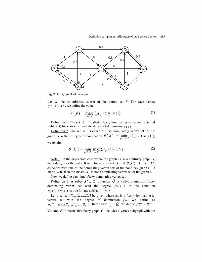
1X

X2

X7

X5

X6

X4

X3

11

1

1

111

1

0,4

0,80,80,8

0,50,5

0,90,9

0,70,7

0,3

Fig. 2. Fuzzy graph of the region

Let ′X be an arbitrary subset of the vertex set X. For each vertex y X X∈ ′\ , we define the value:

,max)( ><=∈

xyy UXxµγ . (1)

Definition 1. The set ′X is called a fuzzy dominating vertex set (external stable set) for vertex y with the degree of domination γ ( )y .

Definition 2. The set ′X is called a fuzzy dominating vertex set for the graph ~G with the degree of domination ).y(min)X(

X\Xyγβ′∈

=′ Using (1),

we obtain:

.,maxmin)(\

><=′′∈′∈

xyX UXxXXyµβ (2)

Note 3. In the degenerate case where the graph ~G is a nonfuzzy graph G, the value β has the value 0 or 1 for any subset ′X . If β( )′ =X 1, then ′X coincides with one of the dominating vertex sets of the nonfuzzy graph G. If β( )′ =X 0, then the subset ′X is not a dominating vertex set of the graph G.

Now we define a minimal fuzzy dominating vertex set. Definition 3. A subset ′ ⊆X X of graph ~G is called a minimal fuzzy

dominating vertex set with the degree β ( )′X if the condition β β( ) ( )′′ < ′X X is true for any subset ′′ ⊂ ′X X .

Let a set τk=Xk1, Xk2,…,Xkl be given where Xki is a fuzzy dominating k-vertex set with the degree of domination βki. We define as

,...,,max 21min

lkkk XXXk ββββ = . In the case ∅=kτ we define minmin

1+=

kk XX ββ .

Volume min

kβ means that fuzzy graph ~G includes k-vertex subgraph with the

Definition of Optimum Allocation of the Service Centres 285

degree of domination min

kβ and doesn’t include k-vertex subgraph with the degree of domination more than min

kβ .

Definition 4. A fuzzy set /,...,2/,1/~ minmin2

min1 ><><><= nB n

xX βββ is

called a domination fuzzy set of fuzzy graph ~G . Property 1. The following proposition is true:

1...0 minmin

2

min

1 =≤≤≤≤ nβββ . We shall conside a task of finding of domination fuzzy set with the given

degree of domination β∈[0,1]. The following algorithm may be propose: 10. For given fuzzy graph ~G and given degree of domination β we

construct crisp subgraph G’=(X,U’), in which edge <x,y>∈U’, if volume βµ >≥< yxU , ;

20. For construct suggraph G’ we define a family of all dominating vertex sets.

The finding family is a family of dominating vertex sets of fuzzy graph ~G which degree of domination more or equal β (for example, by Maghout’s method for nonfuzzy graphs [3]).

We will consider the problem of finding a family of all minimal fuzzy dominating vertex sets with the highest degree. The given method is a generalization of the Maghout’s method for crisp graphs.

Assume that a set T is a fuzzy dominating vertex set of the fuzzy graph ~G with the degree β(T). Then for an arbitrary vertex x Xi ∈ , at least one of the following conditions must be true (or both of them).

a) A vertex x i belongs to the considered set T; b) There is a vertex x j such that it belongs to the set T with the

membership function )(, Txx jiU βµ >≥< . In other words, the following statement is true:

))].(,&)(()[( TxxTxxTxXx jiUjjii βµ >≥<∈∃∨∈∈∀ (3)

To each vertex x Xi ∈ we assign a Boolean variable pi that takes the value 1, if x Ti ∈ and 0 otherwise. We assign a fuzzy variable

><= jiUij xx ,µξ for the proposition )(, Txx jiU βµ >≥< . Passing from the quantifier form of proposition (3) to the form in terms of logical operations, we obtain a true logical proposition:

ΦT i i j j ijp p= ∨∨ =&( ( & )) .ξ 1


Supposing ξ ii = 1 and considering that the equality p p pi j i ij j j ij∨∨ = ∨&ξ ξ is true for any xi , we finally obtain:

Φ T i j ij jp= ∨ =& ( )ξ 1 . (4)

We open the parentheses in the expression (4) and reduce the similar terms using the following rule:

,&&&& xyxx ξξξ ′=′′∨′ for ′ ≥ ′′ξ ξ . (5)

Here, 1,0, ∈yx and ′ ′′ ∈ξ ξ, [ , ]0 1 . Then the expression (4) may be write as:

)&&...&&( 21,1 ikliT apppiii=

∨=Φ . (6)

Property 2. Each disjunctive member in the expression (4) gives a minimal dominating vertex set with the largest degree of domination ai.

Proof. We shall suppose that a following simplification is impossible in the expression (6). Let the disjunctive member

]1,0(,),&&...&&( 21 ∈< ankappp k. (7)

is included into the expression (6). We suppose a subset X’=x1,x2,…,xk isn’t domination set with the degree of domination a. Hence, there is a vertex xk+1∈X/X’ for which the statement ),)(,1( 1 axxki ikU ><<=∀ +µ is true. We rewrite the expression (4) as:

).1...(&... &)...1...(&...&

&)...1(&)...1(

2211

,11,122,111,1

2212112121

nnn

nnkkkkkkk

nnnnT

pppppppp

pppppp

∨∨∨

∨∨∨∨∨∨∨∨∨∨∨=Φ

+++++

ξξξξξξ

ξξξξ (8)

We have kiaik ,1 ,,1 =∀<+ξ in the expression (8). Hence, if disjunctive members in the expression (6) don’t include variables nkk ppp ,...,, 21 ++ then they must include coefficients less than a. Then the disjunctive member (7) can not be included in the expression (6). We obtain the contradiction. Then the subset X’=x1,x2,…,xk is domination set with the domination degree a.

Now we shall prove that the subset X′ is a minimal dominating vertex set. Let us assume that it isn’t true. Then one of the following conditions must

be true. a) The subset X′ is a minimal dominating vertex set with the degree of

domination b>a.


b) There is a dominating vertex subset X′′⊂X′ with the degree of domination a.

Let the condition a) is true. Then the following proposition is true: ),|,1,)(,1,( bxxkixnkjx ijUij >≥<∈∃+=∀ µ .

Let the expression ΦT is presented by (8). If we multiply parentheses without rule (5) then we obtain n2 disjunctive members. Each member contains n elements, one of all parentheses of presentation (8). We select one of n2 disjunctive members by next rule:

- We select the element 1p1 from the first parentheses, the element 1p2 from the second parentheses, …, the element 1pk from the parentheses k. Then we select the element

11,1 iik p+

ξ from the parentheses (k+1) such that the index

i1∈[1,k] and volume bik >+ 1,1ξ , the element

22,2 iik p+

ξ from the parentheses

(k+2) such that the index i2∈[1,k] and volume bik >+ 2,2ξ , …, the element

knkn iin p−− 1,ξ from the parentheses (n) such that the index in-k∈[1,k] and volume

bknin >

− 1,ξ .

Using the rule (5), the obtained disjunctive member may be present as:

)&&...&&( 21 bppp k′ . (9)

In this presentation the volume b′ is defined as abb

kninikik >≥=′−++,...,,min ,,2,1 22

ξξξ . What is why the member (9)

reduces the disjunctive member (7). We obtain the contradiction since the expression (6) contains the disjunctive member (7). This contradiction proves that condition a) is impossible.

Let the condition b) is true. Let the subset X′′ is defined as ,...,, 121 −

=′′ kxxxX . Let the expression ΦT is presented by (8). We select one of n2 disjunctive members by next rule:

- We select the element 1p1 from the first parentheses, the element 1p2 from the second parentheses, …, the element 1pk-1 from the parentheses (k-1). Then we select the element

11, iik pξ from the parentheses (k) such that the index

i1∈[1,k-1] and volume aik ≥1,ξ , the element

22,1 iik p+

ξ from the parentheses

(k+1) such that the index i2∈[1,k-1] and volume aik ≥+ 2,1ξ , …, the element

111, +−+− knkn iin pξ from the parentheses (n) such that the index in-k+1∈[1,k-1] and

volume aknin ≥+− 1,ξ .

Using the rule (5), the obtained disjunctive member may be present as:


)&&...&&( 121 bppp k −. (10)

The volume b is defined as abkninikik ≥=+−+,...,,min

122 ,,1, ξξξ in this

presentation. What is why the member (10) reduces the disjunctive member (7). We obtain the contradiction too. This contradiction proves that condition b) is impossible.

The proof of Property 2 is completed. The following method of foundation of a minimal dominating vertex sets

may be propose on the base of Property 2: - We write proposition (4) for given fuzzy graph ~G ; - We simplify proposition (4) by proposition (5) and present it as

proposition (6); - We define all minimal dominating vertex sets, which correspond the

disjunctive members of proposition (6). Example 2. Find all minimal fuzzy dominating vertex sets for the graph

presented in Fig.2. The corresponding expression (4) for this graph has the following form: ΦT=(p1∨p2∨0,9p3∨0,5p4)&(p1∨p2∨p3∨0,8p4∨0,4p5)&(p1∨0,8p2∨p3∨p4∨0,3p6)& &(0,8p2∨p3∨p4∨0,8p5∨0,9p6∨0,5p7)&(0,4p2∨0,8p4∨p5∨p6∨p7)& &(0,3p3∨p4∨0,7p5∨p6∨p7)&(0,5p4∨0,7p5∨p6∨p7). Using the rule (5), we finally obtain: ΦT =p1p3p6∨p1p4p6∨p2p3p6∨p2p4p6∨p1p3p7∨p1p4p7∨p2p3p7∨p2p4p7∨0,9p1p6∨0,8p2p6 ∨0,9p3p6∨0,8p1p5p7∨0,5p1p7∨0,8p2p7∨0,9p3p7∨0,7p1p5∨0,7p2p5∨0,7p3p5∨0,5p4

. It follows from the last equality that the graph ~G has 19 fuzzy minimal

dominating vertex sets: T1=x1,x3,x6 with the domination degree 1; T2=x1,x6 with the domination degree 0,9; T3=x4 with the domination degree 0,5 and others.

A domination fuzzy set of fuzzy graph ~G is defined as 3/1,2/9,0,1/5,0~ ><><><=XB .

The domination fuzzy set defines the next optimum allocation of the service centres: If we have 3 or 4 service centres then we must place these centres into areas 1, 3 and 6. The degree of service equals 1 in this case. If we have 2 service centres then we must place both centres into areas 3 and 6. The degree of service equals 0,9 in this case. If we have only one service centre then we must place it into area 4. The degree of service equals 0,5 in last case.


3 Conclusion

The task of definition of optimal allocation of the service centres as the task of definition of domination fuzzy set of fuzzy graph was considered. The method of definition of domination fuzzy set is the generalization of Maghout’s method for nonfuzzy graphs. It is necessary to mark that the suggested method is the method of ordered full selection, because these tasks are reduced to the task of covering, i.e. these tasks are NP-compete tasks. However, this method is effective for the graphs which have not homogeneous structure and not large dimensionality. It is necessary to mark too that considered task may be solved by multi-objective performance.

4 Acknowledgements

This work has been supported by the Russian Fond of Fundamental Research project 03-07-90202.

References

1 Bershtein LS, Bozhenuk AV (2001) Maghout Method for Determination of Fuzzy Independent, Dominating Vertex Sets and Fuzzy Graph Kernels. J. General Systems 30: 45-52

2 Kaufmann A (1977) Introduction a la theorie des sous-ensemles flous. Masson, Paris 3 Kaufmann A (1968) Introduction a la combinatorique en vue des applications, Dunod, Paris 4 Christofides N (1975) Graph Theory. An Algorithmic Approach. Academic press,

London


Evolutionary Algorithm of Minimization of Inter-sections and Flat Piling of the Graph Mathematic Models* L.А. Gladkov, V.M. Kureichik Taganrog State University of Radio Engineering [email protected]; [email protected] The problem of minimization of intersections of the graph mathematic models is considered. For its decision evolutionary algorithms are offered. It allows receiving flat piling with local optimum for polynomial time. Complexity of algorithms has a straight-line characteristic.

Introduction

At a solution of different practical problems both of engineering, and eco-nomical nature the special place is occupied with optimization problems grounded on classic graph algorithms, such, for example, as minimization of intersections and constructing of flat piling of the graph, constructing the effective coloring problem of the graph etc.

The mining of the new approaches to a solution of all set forth above problems introduces large concern, both from practical, and scientific point of view. It is conditioned by the fact that the problems of the class NP re-quire large bulk of calculus, and in many cases and an exhaustive search. And the complication even of most simple of them is exponentially grows in accordance with magnification of the number of arguments.

1. Formulation

The relevant aspect of constructing of an effective routine of looking up is the problem of synthesizing the effective architecture.

The genetic algorithms (GA), realizing incidentally - directional policy represent a powerful search tool and determination of optimal solution on set of alternatives. As practice demonstrates, the applying of genetic algo-rithms allows largely to increase performance of accepted solutions at the

* Work is executed at financial support of the Russian Federal Property Fund (the

project 02-01-01275)

expense of usage of the probability rules, necessity of set-up of a search pattern under conditions of a particular problem and possibilities of a choice on each pitch of operation of algorithm from set of invariant alter-natives [1 - 3].

Thus, GA usage is a quality reductant of the architecture of a retrieval system, troubleshoots the realization of discrete reductant.

Usage of methods of evolutionary adapting for realization of the behav-ioral patterns on the basis of principles of changes of aircraft attitude (on Darwin and on Lamarc), natural culling, principle «of survival of the strongest», adapting to variation of conditions of the environment and other, allows to troubleshoot of a continuous component retrieval system [4 - 8].

Each block of the given all-level system relates to a process of decision making, that allows to section a solution of a composite problem into the set of more simple subproblems decided sequentially, pursuant to their hi-erarchy.

The block of analysis and choice of alternatives ensures a choice of the best solution on set of possible alternatives. The choice is carried out de-pending on values of a certain objective function (fitness). The given block realizes functions of discrete component.

The basic problem of the block of teaching and adapting is the concreti-zation of set of equivocations. During operation of the block a teaching of system, takes place owing to what the size of set of equivocations is mod-erated by operation of the block of choice. As the instrument for realiza-tion of trial functions of the block the methods and rules of developmental adapting permitting to model process of progressing of a certain in-trabreeding population of the individuals and adapting them to variation of the environmental conditions with the purpose of survival can be utilised.

The block of teaching and adapting realizes functions of continuous re-ductant, constructing and permanently inflecting a dynamic mock-up of a system behavior at the expense of continuous variation of existing and generation of the new rules of behavior.

2. Minimization of intersections and flat piling of the graph

One of the most laborious graph problems. Many algorithms of minimiza-tion of intersections are known. The genetic algorithm of minimization of intersections, tendered in the present paper, allows not only to execute a

292 Gladkov L.A. and Kureichik V.M.

primal problem, but also to construct in passing alternative of maximal flat piling of the graph on a plain.

The McLain’s theorem is trusted to in a basis of algorithm that the graph can be laid on a plain without intersections, if on set of its cycles it is pos-sible to construct some base Bp, containing p - cycles such, that each edge of the graph strictly belongs to two cycles, where p = m - n + 2 (m - a number of edges, and n - a number of tops of the graph). The basic prob-lem of algorithm is the construction of an optimal solution or sets of solu-tions maximum close to it.

As input data’s the modified agendas of a co occurrence of the graph are used, on a foundation of which one of the generation of a cycle is exe-cuted. The experimental researches held earlier, have shown, that for an one valued solution of a problem it is enough to investigate a set of the most short cycle of the graph, for example, cycles of length 3 - 4, that al-lows to reduce a burn-time of algorithm.

After a termination of process of generation of cycles the routine of an estimation of an amount and a quality of obtained set of cycles is started up. As a result of implementation of the given routine the answer to a problem should be obtained: whether there are enough of available cycles for a solution of a delivered problem or it is necessary to return to the pre-vious routine and to prolong process of generation of cycles. After closing-up of the block of an estimation the generated set of cycles is transmitted to the mainframe of algorithm - block of the genetic operatives (BGO), where a study and generation of a solution takes place.

For a solution of a delivered problem the all-level genetic algorithm conditionally called “building” was designed. The following concept was trusted to in its basis.

The problem of determination of planarity and constructing of flat piling of the graph is esteemed as a problem of constructing of some base fitting to established yardsticks. The building of this base runs in some stages:

1 stage - forming of an original baseline solution. 2 stages - complement of an available baseline solution by new speed

keys of cycles before reaching the greatest possible extent of infill, in an ideal before infill of p - discharges. Depending on reached result the proc-ess is either completed, or the algorithm passes to a following stage.

3 stages - algorithm attempts by singlestep variations to improve an ob-tained earlier solution. In a case if it is possible a process is completed, otherwise algorithm passes to a following stage.

4 stages - obtained solution in an aspect of impossibility of further im-proving is stored, then some modifications are made to the given solution, and the building is iterated from the second stage.

Evolutionary Algorithm of Minimization of Intersections and Flat Piling ... 293

As building methods on the maiden three stages the genetic operatives of selection (operating system), crossover (ОК) and culling (ОC), adapted to specificity a delivered problem are utilized. The problem of adjusting of the design is executed with the help of the operatives of mutation (OM) and inverse (ОI), also modified pursuant to presented requests.

Host material for production of solutions is the earlier formed set of a cycles.

The overall performance of genetic feedback algorithms in many re-spects depends on a method of encoding of datas. With allowance for specificities of a decided problem a special chromosome was proposed, with a number of discharges equal to p + 3. First p of chromosome dis-charges represent numbers of cycles involved in a current solution. The additional three discharges are utilized for estimating the quality of a re-ceivable solution. The discharge p + 1 contains the information about the edges which have been not involved in the given solution, discharge p + 2 - edges involved once and discharge p + 3 - edges, utilized doubly. The values, which can be accepted with a function of estimation (m) are in a spacing [0; 1], and quality of a solution is more, than more the number of edges involved in a valued solution.

In the left-hand half chromosome there can be signifying and insignifi-cant parts. The discharges of a signifying part are spacefilled with numbers of cycles, and insignificant - with zero points, thus, the higher is the qual-ity of a solution, the less is the length of an insignificant part (L0 → 0). An optimal solution L0 will be equal to zero point. I.e. the length of an insig-nificant part is an additional yardstick of quality estimation of the obtained solution.

Thus, the chromosome objective function of an obtained solution (H) is an additive function of two variables: (H) = (δ(m); L0), and f(H) → max, when δ(m) → 2m & L0 → 0.

Different alternatives of forming policy of set of original solutions are foreseen in algorithm.

1. From set of cycles we select edges repeating not more than two times. The cycles, to which one the edges, retrieved as a result of such looking up, belong form a speed key representing an original solution. If there are edges in it repeating more than 2 times, the minimum possible number of cycles containing “superfluous” edges is removed from a speed key and a speed key will be converted into chromosome.

2. The original baseline solution is reshaped at the expense of join of cycles, incidentally selected pair of cycles having as the minimum one common edge.


3. The original baseline solution is reshaped at the expense of series at-tachment as long as there is such a possibility, or the clandestine solution will not be derivated yet.

If there are the applicable technical facilities rather effective is a macro-evolution principle usage, when two or more populations are in bridge re-shaped and developed with periodic interpopulation information exchange.

The set of the interlocutory orders is reshaped by cycle joining having identical edges. And numbers of thus receivable pair edges necessarily should coincide with numbers of edges written in discharges p + 1 or p + 2 baseline original solution. Besides, cycle numbers from set of the inter-locutory orders should not coincide with cycle numbers of a participating in a baseline solution. The size of a population of the interlocutory orders depends on quality of an original solution or is set by the user.

After creation of set of the interlocutory orders, the selection for a choice of solutions participating in operation of a crossing-over (ОК) is executed. For this purpose the following rules should be executed:

1. Minimum number of concurrences of numbers of edges in discharges p + 2 and p + 3 of challenger and discharge p + 3 of parents.

2. Maximal number of identical edges in discharge p + 1 of challenger and discharge p + 3 of first parents.

3. Maximal number of concurrences of edges from p + 2 of challenger with edges from discharge p + 2 of the first parent chromosome.

On the basis of datas of the rules special all-up argument - function of operability of the interlocutory orders concerning a baseline solution f’(H) was designed. The quantitative value of function of operability is counted on the basis of counting number concurrence of numbers of edges in dif-ferent chromosome discharges.

The improving of an original baseline solution is made with the help of the modified operative of a crossover (ОК), for the purpose of that from set of the interlocutory orders the member having the best function of op-erability concerning the maiden parent is selected and is assigned for im-plementation ОК. The dots of a continuous twist in such ОК are selected as follows:

1. In the 1st parent 1st the dot of a continuous twist t1 is always behind the latter signifying (nonzero) chromosome element hi, 2nd the dot t2 is se-lected after a member hi + k, where k – is number of signifying element in 2 mother chromosome.

2. In the 2nd parent the 1st dot is always before the 1st chromosome ele-ment, and the 2nd dot is defined as well as in a case with the 1st parent.

As a result of implementation of ОК there is a join of signifying parts of parents chromosomes. If a function of operability of the second parent δ’m(H) ≠ 1, them from chromosomes of the descendant an edge (or edges),


repeating in the given speed key more than two time are removed. In bridge with removal of edges Nc - cycle are removed to which the given edge belongs. However again appeared in chromosome a cycle can not be deleted.

After ОК implementation the count of functions of operability of all in-terlocutory orders concerning a new baseline solution is made and the so-lutions having negative estimations are removed from a population.

At deriving a solution not producing improving during considerable number of breeds, the operations of mutation and inverse are applied to it. For this purpose the casual image selects two discharges (signifying and insignificant). After interchanging the signifying member is zeroed, and all edges, inhering to the given cycle, are removed from genes p + 2 and p + 3. The schema of a fulfilling of an operation of inverse is similar to opera-tion of mutation with the only variance, that for interchanging not one gene chromosome, is selected but a few. The number of interchanged genes is set by a casual image, however it should not be more then the numbers of insignificant discharges of inverted chromosome.

After chromosome deciphering with the help of the block of flat piling it is possible to scan alternatives of piling of the graph on a plain without in-tersections.

3. Results of experimental research

The developed algorithm is effective for the decision optimization prob-lems of definition of planar of graphs models, revealing of the maximal planar part the column and constructions of its flat stacking. The algorithm has polinomial time complexity that proves to be true the received experi-mental results. The algorithm is realized as the program appendix in pro-gramming language C ++ with use of environments of programming Bor-land C ++ Builder 6.0 and Visual C ++ 7.0. Testing of the developed program was made on personal computers such as IBM PC c by processors Athlon XP 1700 - 2100 and Pentium IV. On the basis of the received data schedules of dependences of time and quality of received decisions from value of dimension of entrance given and basic adjustmentsoptions of algorithm are constructed.

At carrying out of experimental researches of the developed algorithm three were used graph models: G1 (25 nodes, 60 edges), G2 (50 nodes, 120 edges) и G3 (65 nodes, 130 edges). (Tab. 1).


Table 1. Results of experimental researches

K Np Br Lo Bc T(G1) T(G2) T(G3) 25 50 10 5 5 6.99 13.46 15,11 25 100 10 5 5 11.98 19.95 23,24 25 50 20 2 2 7.87 9.85 12,3 25 100 20 2 2 13.9 10.11 21,27 50 50 10 5 5 14.45 9,62 26,98 50 100 10 5 5 25.94 10,11 44,11 50 50 20 2 2 14.95 27,42 24,4 50 100 20 2 2 27.58 37,25 42,46 100 30 10 5 5 19.46 62,1 33,95 100 50 10 5 5 29.62 54,83 48,44 100 100 10 5 5 55.92 65,65 91,63 100 30 20 4 4 18.4 140,29 30,38 100 50 20 4 4 32.2 142,75 46,59 100 100 20 4 4 56.86 137,88 88,66

K - quantity of iterations; Np - the size of a population; Br - number of base decisions; Lo - number of steps for definition of a local optimum; Bc - number of steps for allocation of normal basis of cycles; T(G1 – G3) - operating time of algorithm.

P

t(сек.)

10 20 30 40 50 60 70 80 90 100

10

20

30

40

50

I

II

III

Fig. 1. Dependence diagram of an operating time of algorithm from the size of a population

On fig.1 the schedule reflecting dependence of an operating time of al-gorithm on the size of a population of intermediate decisions is shown.

The conclusion

Designed algorithms has a straight-line characteristic of temporary com-plication. For study GA the system of the test problems (benchmarks) was designed, intended for matching GA with other techniques and the unique-ness of capacities GA for problem solving of optimization is demonstrated.


However is apparent, that at an exterior simplicity GA require considerable efforts on set-up under a particular problem. Probably, it is meaningful to speak not about complication of applying GA in general, but about ade-quacy of levels of complication of algorithm and decided problem. The easier problem, the more senseless are different shifts with the coding of genotypes, set-up of odds etc. In case if the fitness has an alone extremum in investigated field, the applying of GA loses any sense, since any local method will discover a solution faster and easier. On the other hand, it is impossible to tell, that there is no such a problem, which could not be de-cided with the help of GA.

References

1. Kureichik V.М. Genetic algorithms: the Monography. Taganrog: Publishing house TRTU, 1998.

2. Emeljanov V.V., Kureichik V.V., Kureichik V.M. Theory and practice of evo-lution simulation. – Moscow: “Phismatlit”, 2003.

3. Batishchev D.A. Genetic algorithms of the decision of extreme problems. Vo-ronezh: Publishing house VGTU, 1995.

4. Holland, John H., Adaptation in Natural and Artificial Systems: An Introduc-tory Analysis with Application to Biology, Control, and Artificial Intelli-gence. University of Michigan, 1975.

5. Handbook of Genetic Algorithms. Edited by Lawrence Davis, Van Nostrand Reinhold, New York, 1991.

6. Practical Handbook of Genetic Algorithms. Applications. Volume 1. Edited by Lawrence D. Chambers. - CRC Press. Boca Raton, London, New York, Washington, D.C., 1995 – 1999

7. Tokinaga S., Yakabe M. An Evolutional Approach to the Control of Chaotic Economic Dynamics. // Proceeding of 2000 International Symposium of Nonlinear Theory and Applications. - Dresden, Germany, 2000. - p. 181 - 185.

8. Tokinaga S., Yakabe M. An Evolutional Approach to the Control of Chaotic Economic Dynamics. // Proceeding of 2000 International Symposium of Nonlinear Theory and Applications. - Dresden, Germany, 2000. - p. 181 - 185.


Use of a fuzzy strategy to create the shortest Hamiltonian cycle

Henryk Piech , Aleksandra Ptak

Technical University of Czestochowa, Institute of Mathematics and Infor-matics, tel. 604559300, e-mail:hpiech.adm. pcz.czest.pl, ul. Dabrowskiego 73

Summary

Hamiltonian cycles, which are a basis of many algebraic analysis meth-ods, as a rule, are subjected to procedures of minimization of their length. Such an approach is characteristic in many problems like: transport (the travelling salesman’s problem), network, flow and structural problems. Most often non-directed graphs are met with in which the shortest distance between two nodes is even. The use of fuzzy strategy inference problems can be for example reduced to the selection of the successive added node to a Hamiltonian cycle using its adaptive abilities to the existing structure of connections. Thus, characteristics of the proposed node will be consid-ered together with parameters of the created structure. There is also a pos-sibility to use non-deterministic methods (e.g. genetic algorithms) which are controlled by means of fuzzy characteristics (belonging function, pre-disposition function or clearance function). Such possibilities from algo-rithmization and the approach of the optimal solutions perspective will be considered in this paper.

Key words: Hamiltonian cycle, logic and fuzzy modelling, genetic algorithms.

Assumptions and conceptions of the algorithmization of the approximative methods of Hamiltonian cycle length minimization

The basic assumption concerning the cycle (a shortened definition which will be used with reference to the Hamiltonian cycle) is obviously the participation of all graph nodes in it. Another assumption concerns the distances between nodes, and can be formulated as follows:

1. the distance between nodes A and B is the same as between nodes B and A (thus, a non-directed graph will probably have to be dealt with),

2. the distances between A and B nodes are different in both directions.

The existing methods of creating a cycle with the minimum length are mainly based on a construction of the shortest subspanning tree algorithm. These methods can be rated among approximative groups which do not give a guarantee of the optimal solution obtainment. Figure 1 presents an example of the obtained solution thanks to the use of such a method. Table 1 contains the data for this example that represent distances between all nodes for the non-directed graph construction.

Table 1. Distances between nodes in the non-directed graph 1 2 3 4 5 6 1 0 33 26 2 34 22 2 33 0 15 21 41 5 3 26 15 0 27 7 19 4 2 21 27 0 53 26 5 34 41 7 53 0 25 6 22 5 19 26 25 0

1. initial node: 1

No. 1 4 2 6 3 5 S↓

From 2 21 5 19 7 34 88

300 Piech Henryk and Ptak Aleksandra

2. initial node: 3

Fig. 1. Creating the two “minimized” Hamiltonian cycles for the initial points: No.1 and No.3 with use of the shortest subspanning tree algorithm (No. – number of associated node, From – metric added to the cycle, S↓ denotes the total cycle length)

No. 3 2 6 1 4 5 S↓↓ From 15 5 22 2 53 7 104

No.1

No.4

No.2

No.6 No.3

No.5

No.3

No.2

No.6

No.1

No.1

No.5

Use of a fuzzy strategy to create the shortest Hamiltonian cycle 301

Adding the shortest arcs to the already existing graphic structure creates the shortest subspanning tree, on condition that they do not create a cycle [10]. In other words, it will be adding a new node which is at the shortest distance from the already built tree.

It is common knowledge that using the shortest subspanning tree method for the shortest Hamiltonian cycle search does not give the optimal solution [10]. The best result obtained in example (see Table 1), using all nodes as start points, amounts to 88, whereas the optimal solution gives 86.

An inclusion of the above described conceptions based on modifications of the approximative method in algorithmic comparative analysis is pro-posed in this paper. These modifications consist of: − replacement of the minimal subspanning tree by the shortest single

linked list or − replacement of the minimal subspanning tree by the shortest double

linked list.

The shortest single linked list is created by adding to the last node another which is in the shortest distance. In the double linked list, however, the successive nodes are added so that they are at the shortest distance from both list ends. Considering the fact that a by-pass of the subspanning tree or lockup of the list requires the addition of the last segment which is ended at the start point (what can to a crucial extent influence the quality of solution, that is, the cycle length) one is forced to use all possible start points for the analy-sis. The results obtained for both conceptions of the shortest Hamiltonian cycles searching are quoted below. The series of investigations have demonstrated 67% effectiveness in find-ing the optimal solution with the shortest single linked list method and 64% effectiveness by means of the double linked list. The use of the single linked list gave the optimal result (86), however, the use of the double linked list gave the result close to but not equal to the optimal (88). Both methods can be counted among approximate methods similar in the algo-rithm operation and also in the obtained effects of the method based on the shortest subspanning tree.


1 2 3 4 5 6 S1

0 5

10 15 20 25 30 35 d

istance

succesive connection

comparison of two methods for creating the Hamiltonian cycle

1 2 3 4 5 6

S10

102030405060

dis

tan

ce

successive connections


S1=104 S2=104

S1,2=88


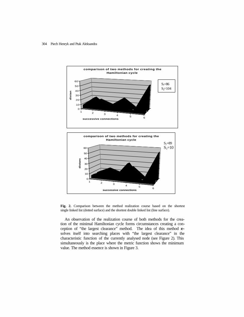
Fig. 2. Comparison between the method realization course based on the shortest single linked list (dotted surface) and the shortest double linked list (line surface).

An observation of the realization course of both methods for the crea-tion of the minimal Hamiltonian cycle forms circumstances creating a con-ception of “the largest clearance” method. The idea of this method re-solves itself into searching places with “the largest clearance” in the characteristic function of the currently analysed node (see Figure 2). This simultaneously is the place where the metric function shows the minimum value. The method essence is shown in Figure 3.

1 2 3 4 5 6

S1S20

10

20

30

40

50

60

dis

tan

ce



S1=86 S2=104

1 2 3 4 5 6

S1S20

10

20

30

40

50

60

dis

tan

ce



S1=89 S2=10


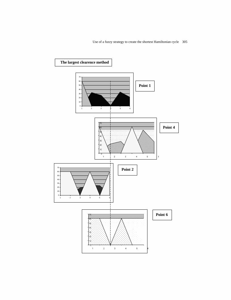
0

10

20

30

40

50

60

70

1 2 3 4 5 6

0

10

20

30

40

50

60

70

1 2 3 4 5 6

The largest clearence method

0

10

20

30

40

50

60

70

1 2 3 4 5 6

Point 1

Point 4

0

10

20

30

40

50

60

70

1 2 3 4 5 6

Point 2

Point 6


ig. 3. Graphic convention of “the largest clearance” method applied for the search-ing of the shortest Hamiltonian cycle

Description of “the largest clearance” method: 1. Assignation of the selection schedule of successive nodes as start points. 2. Description of the metric function from remaining nodes for the succes-

sive point (start or successive added to the list) - see Figure 6 for the metric function denotation (line surface)

3. Description of the blocking function for added nodes to the structure of the single- and double linked list - see Figure 6 for the blocking function denotation (dotted surface).

4. Search of the “clearance” quantity in the structure of the superimposed metric and blocking functions.

5. Selection of the new node in the place of “the largest clearance” of the superimposed metric and blocking functions.

6. Return to point 2 or end of the list creating the procedure in case of the all added nodes.

Point 3

0 10 20 30 40 50 60 70

1 2 3 4 5 6

Point 5

0

10

20

30

40

50

60

70

1 2 3 4 5 6


7. Start of search for the next start point when the list creation for a given point is completed.

References

[1] Czogala E., Perdycz W.: Elements and methods of fuzzy sets theory. PWN, Warsaw 1985 (in Polish)

[2] Davis L.: Genetic Algorithms and Simulated. A. Morgan Kaufmann Pub. Inc., 1988

[3] Davis L.: Handbook of Genetic Algorithms. Nostrand Reinhold, 1991 [4] De Groot M. H.: Optimal statistic decisions. McGraw – Hill, New

York 1970 [5] Kacprzyk J.: Fuzzy sets in system analysis. PWN, Warsaw 1986 (in

Polish) [6] Lachwa A.: Fuzzy world of files, numbers, relations, facts, rules and

decisions. Akademicka Oficyna Wydawnicza Exit, Warsaw 2001 (in Polish)

[7] Lorayane H.: Secrets of supermemory. RAVI, Warsaw 2002 (in Pol-ish)

[8] Piegat A.: Fuzzy modelling and controlling. Akademicka Oficyna Wydawnicza Exit, Warsaw 2003 (in Polish)

[9] Rutkowska D., Piliñski M., Rutkowski L.: Neural networks, genetic algorithms and fuzzy systems, WN PWN, Warsaw 1997 (in Polish)

[10] Sys³o M.M.,Deo N.,Kowalik J.S.: Discrete Optimalization Al-gorythms , WNT,1995.

[11] Zadeh L. A.: Fuzzy limitations calculus; design and systems; meth-odological problems. Ossolineum 1980 (in Polish)


Author Index

Abaoub Ezzeddine 378 Ahmed Uzair 89 Ahrameiko Alexey A. 360 Akbarov R.M. 332 Ali Arshad 89 Aliev R.A. 368 Alpatsky V.V. 403 Anikin I.V. 202 Augustin Thomas 186 Barbouch Rym 378 Batyrshin I.I. 170 Batyrshin I.Z. 39, 62, 73, 122, 170 Belluce Peter 265 Berbasova Natalya Y. 360 Bershtein Leonid 283 Bikesheva Gulnara 210 Borisov Arkady 33, 210, 466 Bozhenyuk Alexander 283 Canfora Gerardo 457 Charfeddine Souhir 350 Cornelis Chris 54 Correa da Rosa Joel 230 D'Alessandro Vincenzo 457 Davnis V.V. 578 De Baets Bernard 3, 162 De Cock Martine 54 De Coligny Marc 350 De Meyer Hans 3, 162 De Schuymery Bart 162 Di Nola Antonio 265 Dounias Georgios 103 Dymova L. 549

Emelyanov Viktor V. 311 Gilmutdinov R. 538 Gladkov L.A. 291 Glova V.I. 202 Gonera M. 549 Grabisch Michel 154 Grishina Е. N. 493 Herrera-Avelar R. 39, 62, 73 Hirota Kaouru 35 Imanov Q.C. 332 Ionin V.K. 257 Ismagilov I. 394 Jain V. K. 194 Jończyk M. 484 Kacprzyk Janusz 501 Kaino Toshihiro 35 Karpov Yury 557 Katasev A.S. 202 Kerre Etienne 54 Kitchens Fred L. 386 Klimova Angelica 122, 130 Kokosh A. 423 Korchunov Valentin 474 Korolkov Mikhail 521 Kuchta Dorota 438 Kureichik V.M. 249, 291 Kureichik V.V. 249

Lajbcygier Paul 97 Leks Dariusz 570 Lettieri Ada 265 Lyubimov Boris 557 Mamedov F.C. 332 Mammadli S. F. 368 Marček Dušan 81 Mareš Milan 143 Medeiros Marcelo 230 Mora-Camino Félix 350 Muzzioli Silvia 222 Nedosekin A.O. 403, 423, 474, 521, 557 Neocleous Costas 340 Pankevich Olga 103 Pheoktistov O.N 202 Piech Henryk 299, 570 Pinto Dias Alves Antonio 446 Plesniewicz G.S. 257 Ptak Aleksandra 299 Reynaerts Huguette 222 Rocha-Mier Luis 321 Rozenberg Igor 283 Rozenberg P. 415 Rubtsov A.V. 394 Rudas T. 122 Ruta Dymitr 111 Ryjov Alexander 511 Salakhutdinov R.Z. 394 Schizas Christos 340 Segeda Anna 521 Sergei V. Ivliev 565 Sevastianov P. 415, 484, 549

Sheremetov L. 39, 62, 73, 321 Shtovba Serhiy 103 Siniavskaya Olga A. 360 Sitarz Sebastian 238 Suarez R. 39, 62, 73 Tarassov Valery B. 272 Tinyakova V.I. 578 Troiano Luigi 457 Trzaskalik Tadeusz 238 Utkin Lev V. 178, 186 Valishevsky Alexander 466 Veiga Alvaro 230 Velisava T. Sevrouk 565 Villareal Francisco 321 Wyrzykowski R. 549 Yahya Asjad 97 Yarushkina Nadezhda 530 Yazenin A.V. 16 Zadrożny Slawomir 501 Zaheeruddin 194 Zaib Gul 89 Zhelezko Boris A. 360

Documents

International Conference on Fuzzy Sets and Soft Computing ... · International Conference on Fuzzy Sets and Soft Computing in Economics and Finance FSSCEF 2004 Proceedings Volume