Intro to Ecology

Scope of Ecology

• Ecology is the scientific study of the interactions between organisms and the environment.

• These interactions determine distribution of organisms and their abundance

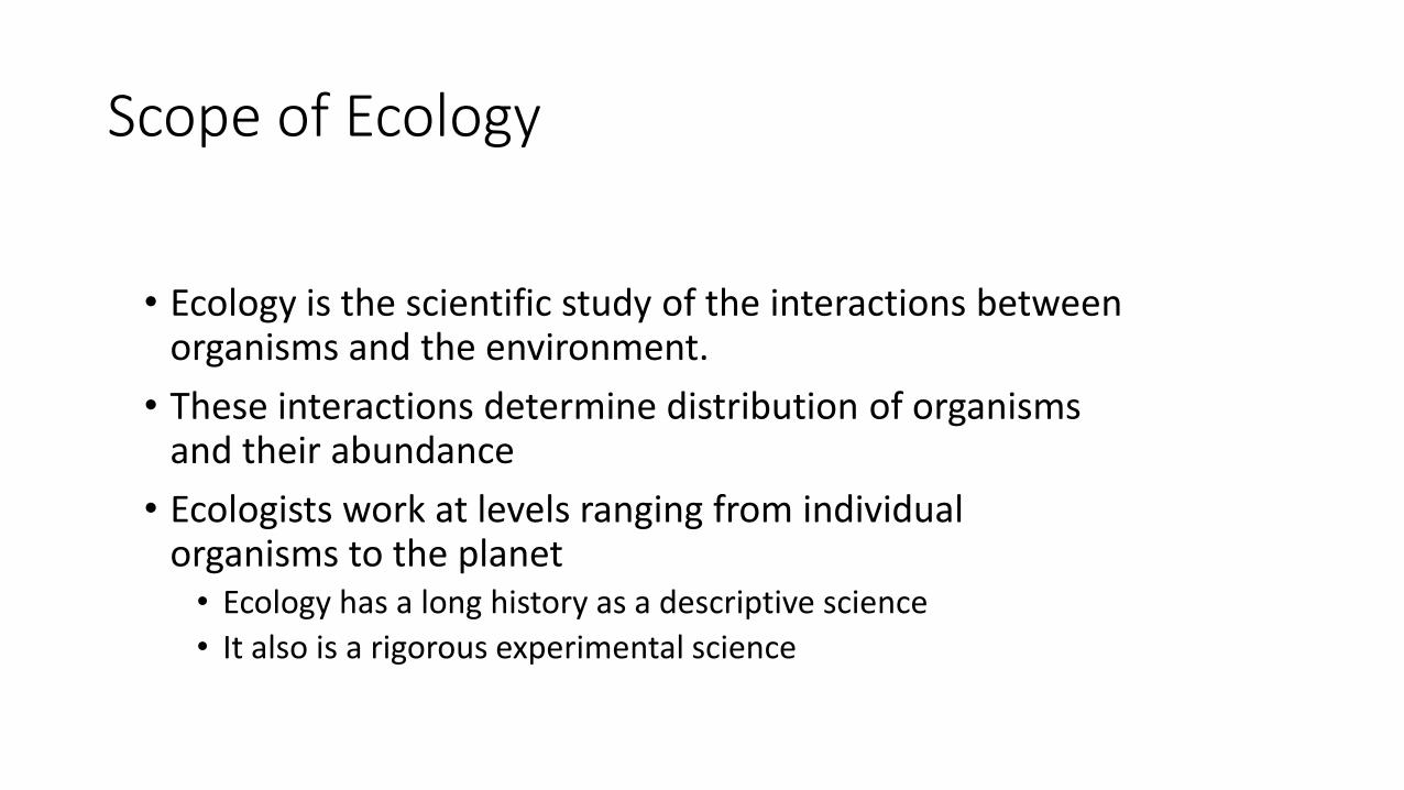
• Ecologists work at levels ranging from individual organisms to the planet• Ecology has a long history as a descriptive science

• It also is a rigorous experimental science

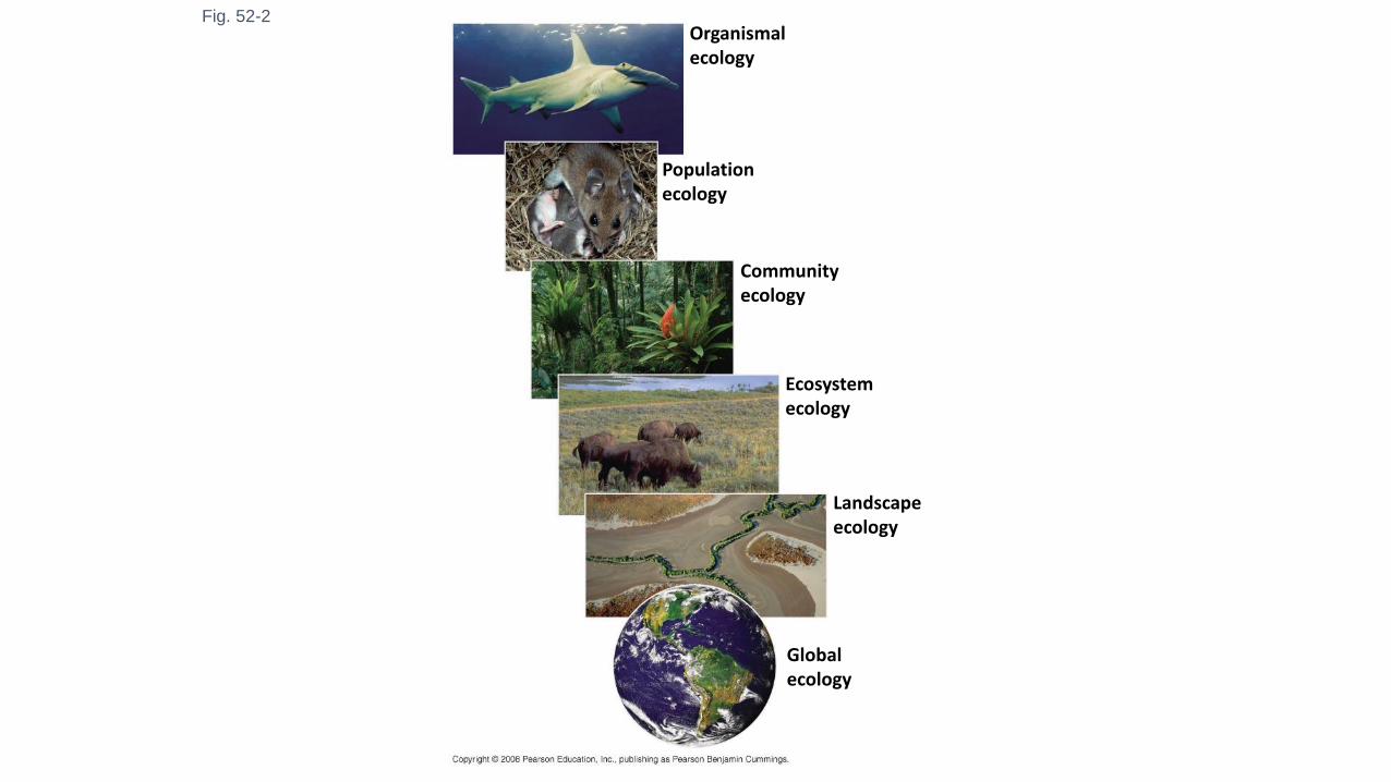
Fig. 52-2Organismalecology

Populationecology

Communityecology

Ecosystemecology

Landscapeecology

Globalecology

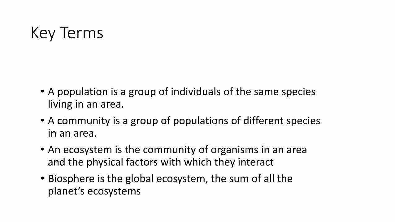
Key Terms

• A population is a group of individuals of the same species living in an area.

• A community is a group of populations of different species in an area.

• An ecosystem is the community of organisms in an area and the physical factors with which they interact

• Biosphere is the global ecosystem, the sum of all the planet’s ecosystems

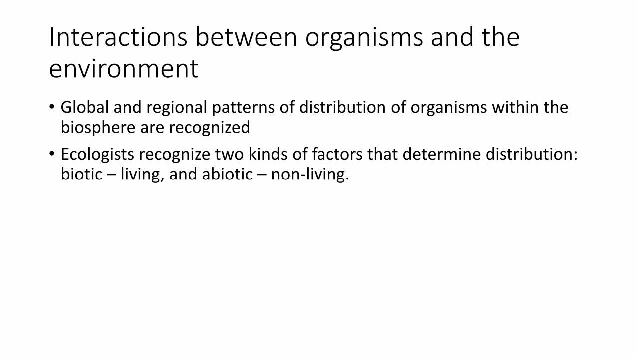
Interactions between organisms and the environment• Global and regional patterns of distribution of organisms within the

biosphere are recognized

• Ecologists recognize two kinds of factors that determine distribution: biotic – living, and abiotic – non-living.

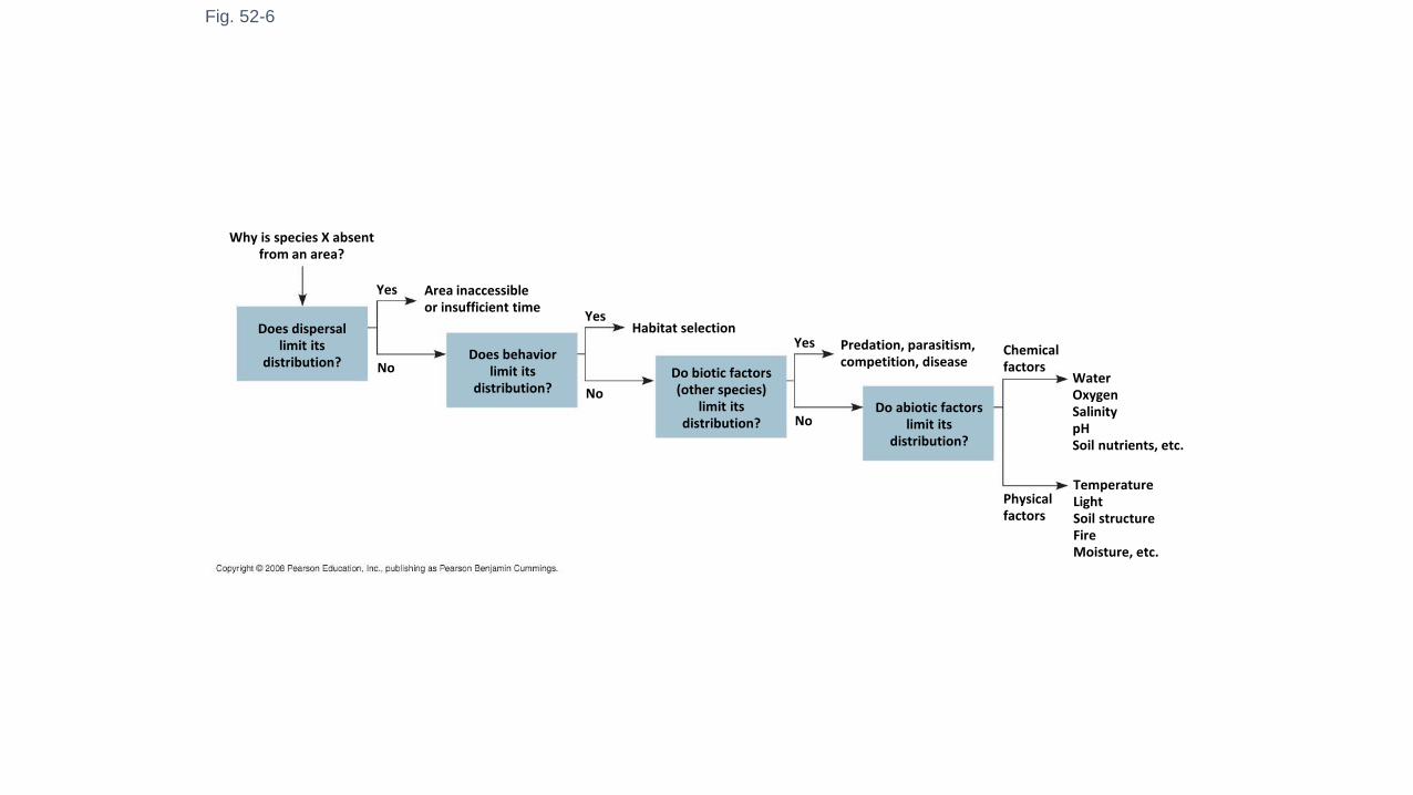
Fig. 52-6

Why is species X absentfrom an area?

Does dispersallimit its

distribution?Does behavior

limit itsdistribution?

Area inaccessibleor insufficient time

Yes

No

No

No

Yes

YesHabitat selection

Do biotic factors(other species)

limit itsdistribution?

Predation, parasitism,competition, disease

Do abiotic factorslimit its

distribution?

Chemicalfactors

Physicalfactors

WaterOxygenSalinitypHSoil nutrients, etc.

TemperatureLightSoil structureFireMoisture, etc.

• Dispersal is the movement of individuals away from centres of high pop’n density or from their area of origin. This contributes to global distribution of organisms.

• Natural range expansions show the influence of dispersal on distribution

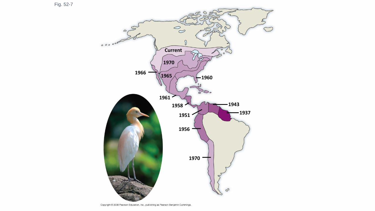
Fig. 52-7

Current

1966

1970

1965 1960

1961

1958

1951

1943

1937

1956

1970

• Species transplants include organisms that are intentionally or accidentally relocated from their original distribution.

• Species transplants can disrupt ecosystems to which they have been introduced

• Some organisms do not occupy all of their potential range

• Species distribution may be limited by habitat selection behavior

• Biotic factors that affect distribution may include:• Interactions with other species

• Predation

• competition

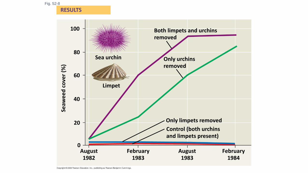
Fig. 52-8

RESULTS

Sea urchin

100

80

60

40

20

0

Limpet

Seaw

ee

d c

ove

r (%

)

Both limpets and urchinsremoved

Only urchinsremoved

Only limpets removed

Control (both urchinsand limpets present)

August1982

August1983

February1983

February1984

• Abiotic factors affecting distribution of organisms include:• Tempurature

• Water

• Sunlight

• Wind

• Rocks and soil

• Most abiotic factors vary in space and time

Tempurature

• Enviro temperature is an important factor in distribution of organisms because of its effects on biological processes

• Cells may freeze and rupture below 0°C, while most proteins denature above 45°C

• Mammals and birds expend energy to regulate their internal temp

• Water availability• For example desert organisms exhibit adaptations for water conservation

• Salinity affects water balance of organisms through osmosis• For example few terrestrial organisms are adapted to high-salinity habitats

Sunlight

• Light intensity and quality affect photosynthesis

• Water absorbs light, meaning in aquatic enviros most photosynthesis occurs near surface

• In deserts, high light levels increase temp and can stress organims

Rocks and Soil

• Many characteristics of soil limit distribution of plants and thus the animals that feed upon them:• Physical structure

• pH

• Mineral composition

Climate

• 4 major abiotic components of climate are temp, water, sunlight, and wind

• Climate is the long-term prevailing weather conditions

• Macroclimate – patterns on the global, regional, and local level

• Microclimate – very fine patterns within a community such as organisms under a fallen log

Global Climate Patterns

• Global climate patterns are determined largely by solar energy and the planet’s movement in space• Sunlight intensity

• Tropics – more heat and light than higher latitudes

• Seasonal variations of light and temp increase steadily toward the poles

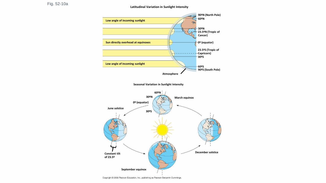
Fig. 52-10aLatitudinal Variation in Sunlight Intensity

Low angle of incoming sunlight

Sun directly overhead at equinoxes

Low angle of incoming sunlight

Atmosphere

90ºS (South Pole)60ºS

30ºS

23.5ºS (Tropic ofCapricorn)

0º (equator)

30ºN23.5ºN (Tropic ofCancer)

60ºN90ºN (North Pole)

Seasonal Variation in Sunlight Intensity

60ºN

30ºN

30ºS

0º (equator)

March equinox

June solstice

Constant tiltof 23.5º

September equinox

December solstice

• Global air circulation and precipitation patterns play major roles in determining climate patterns

• Warm wet air flows from the tropics toward the poles

Fig. 52-10dGlobal Air Circulation and Precipitation Patterns

60ºN

30ºN

0º (equator)

30ºS

60ºS

Global Wind Patterns

Descendingdry airabsorbsmoisture

Ascendingmoist airreleasesmoisture

Descendingdry airabsorbsmoisture

Aridzone

Tropics Aridzone

0º

66.5ºN(Arctic Circle)

60ºN

30ºN

0º(equator)

30ºS

60ºS66.5ºS(Antarctic Circle)

Westerlies

Northeast trades

Doldrums

Southeast trades

Westerlies

23.5º30º 23.5º 30º

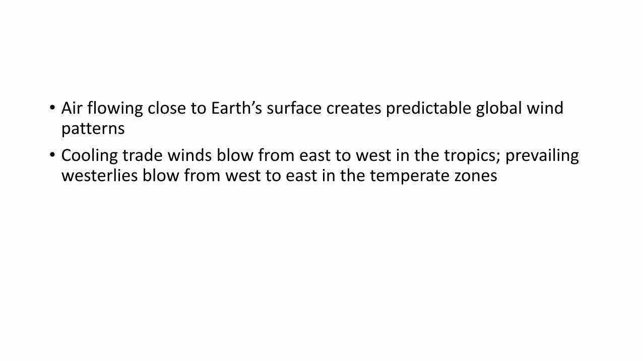
• Air flowing close to Earth’s surface creates predictable global wind patterns

• Cooling trade winds blow from east to west in the tropics; prevailing westerlies blow from west to east in the temperate zones

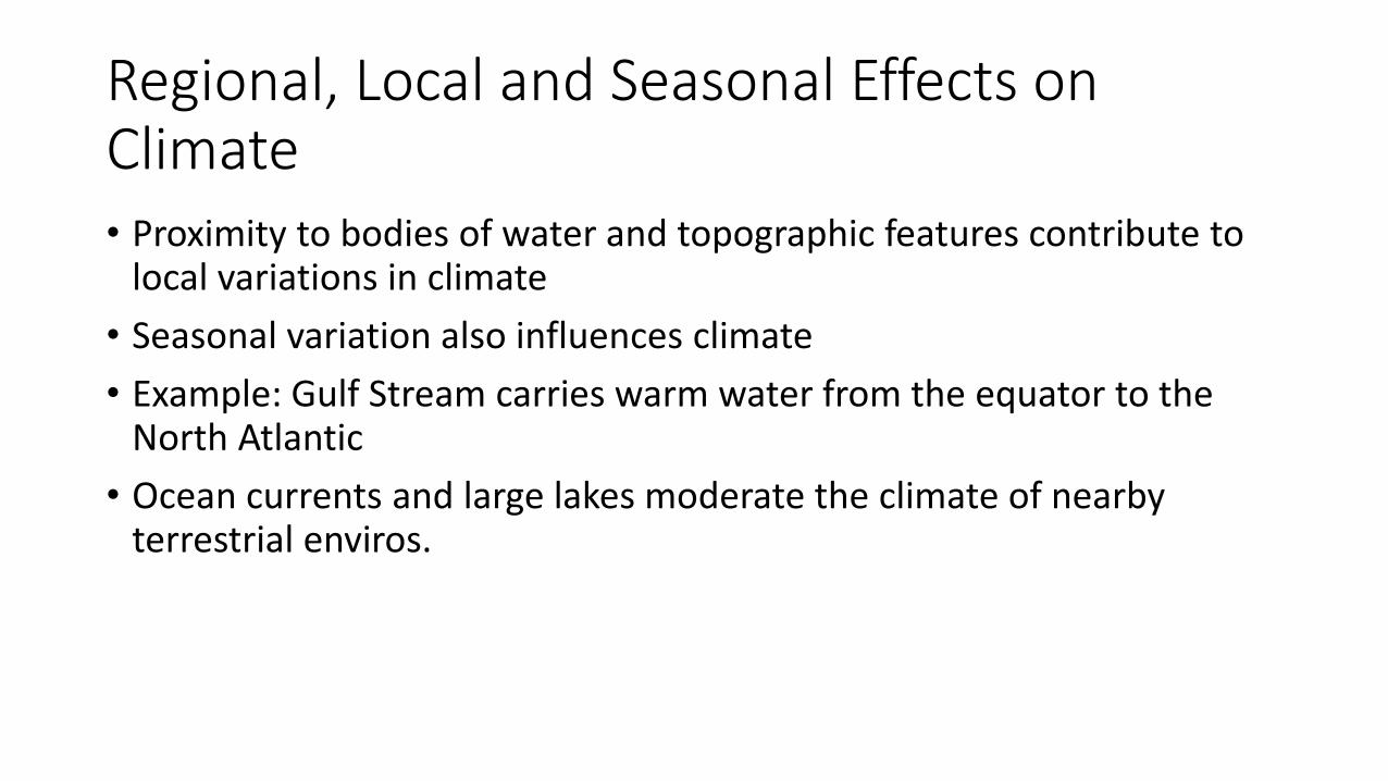
Regional, Local and Seasonal Effects on Climate• Proximity to bodies of water and topographic features contribute to

local variations in climate

• Seasonal variation also influences climate

• Example: Gulf Stream carries warm water from the equator to the North Atlantic

• Ocean currents and large lakes moderate the climate of nearby terrestrial enviros.

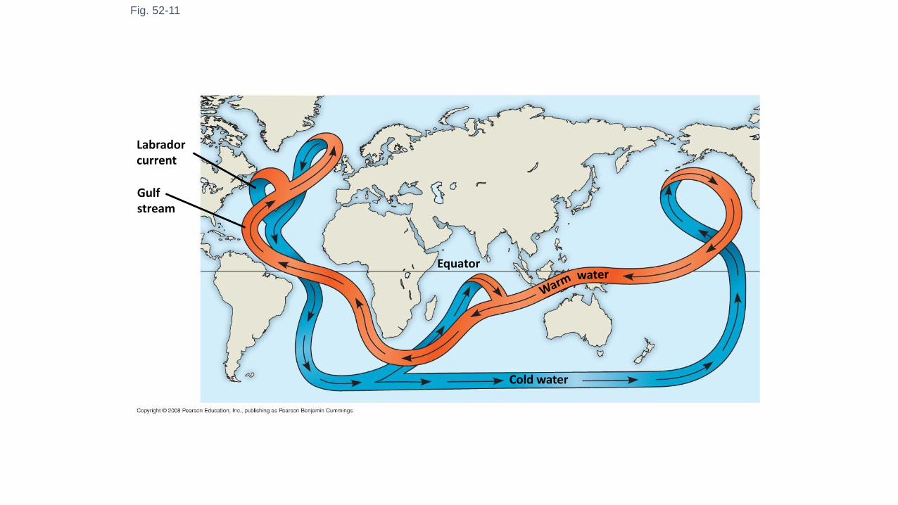
Fig. 52-11

Labradorcurrent

Gulfstream

Equator

Cold water

• During the day, air rise over warm land and draws a cool breeze from the water across the land

• As the land cools at night, air rises over the warmer water and draws cooler air from land back over the water, which is replaced by warm air from offshore

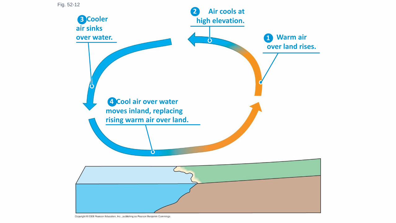
Fig. 52-12

Warm airover land rises.1

23

4

Air cools athigh elevation.

Cool air over watermoves inland, replacingrising warm air over land.

Coolerair sinksover water.

Mountains

• Mountains have significant effect on• Amount of sunlight reaching an area

• Local temp

• Rainfall• Rising air releases moisture on the windward side of peak and creates a “rain shadow” as

it absorbs moisture on the leeward side

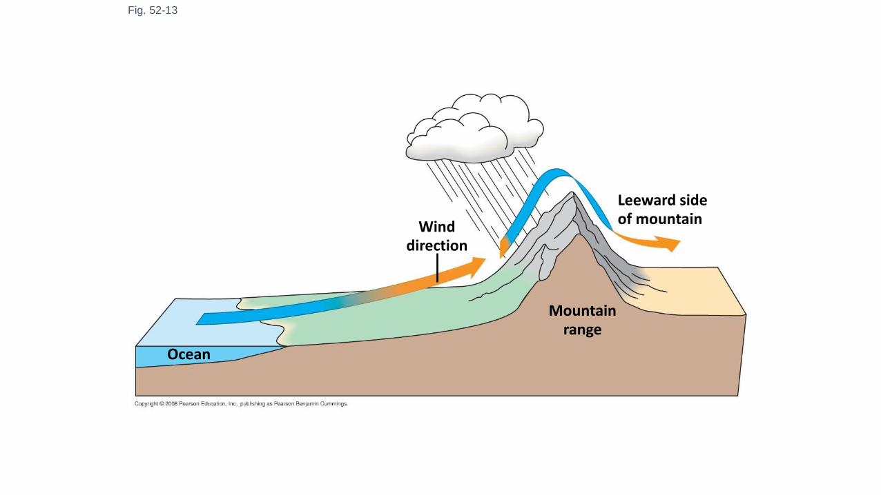
Fig. 52-13

Winddirection

Mountainrange

Leeward sideof mountain

Ocean

Seasonality

• The angle of the sun leads to many seasonal changes in local enviros

• Lakes are sensitive to seasonal temperature change and experience seasonal turnover

Microclimate

• Microclimate is determined by fine-scale differences in the enviro that affect light and wind patterns

Population Ecology

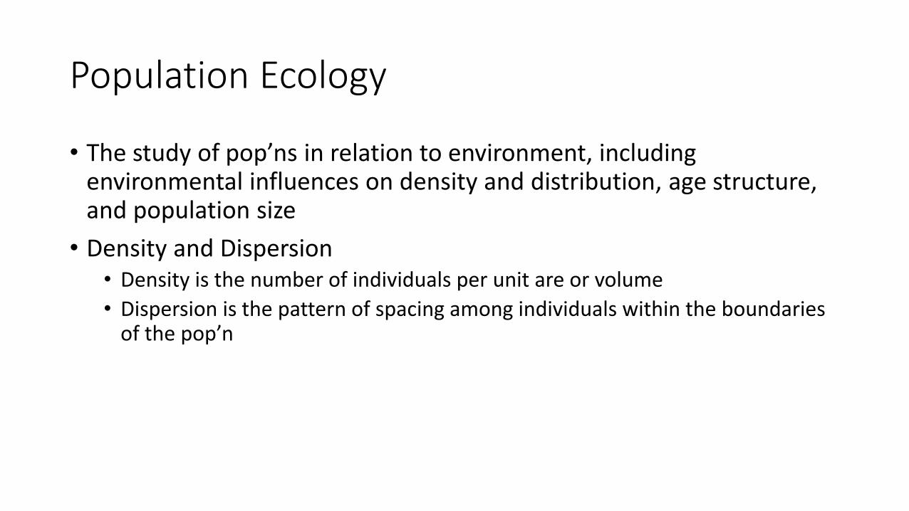
• The study of pop’ns in relation to environment, including environmental influences on density and distribution, age structure, and population size

• Density and Dispersion• Density is the number of individuals per unit are or volume

• Dispersion is the pattern of spacing among individuals within the boundaries of the pop’n

Estimating population sizes

• In most cases, it is impossible to count all individuals in a pop’n

• Sampling techniques can be used to estimate densities and total pop’n sizes

• Population size can be estimated by either extrapolation from small samples, and index or population size, or the mark-recapture method

Factors that add and remove individuals to a pop’n• Immigration – new individuals from other areas

• Emigration – movement of individuals out of a pop’n

• Births

• Deaths

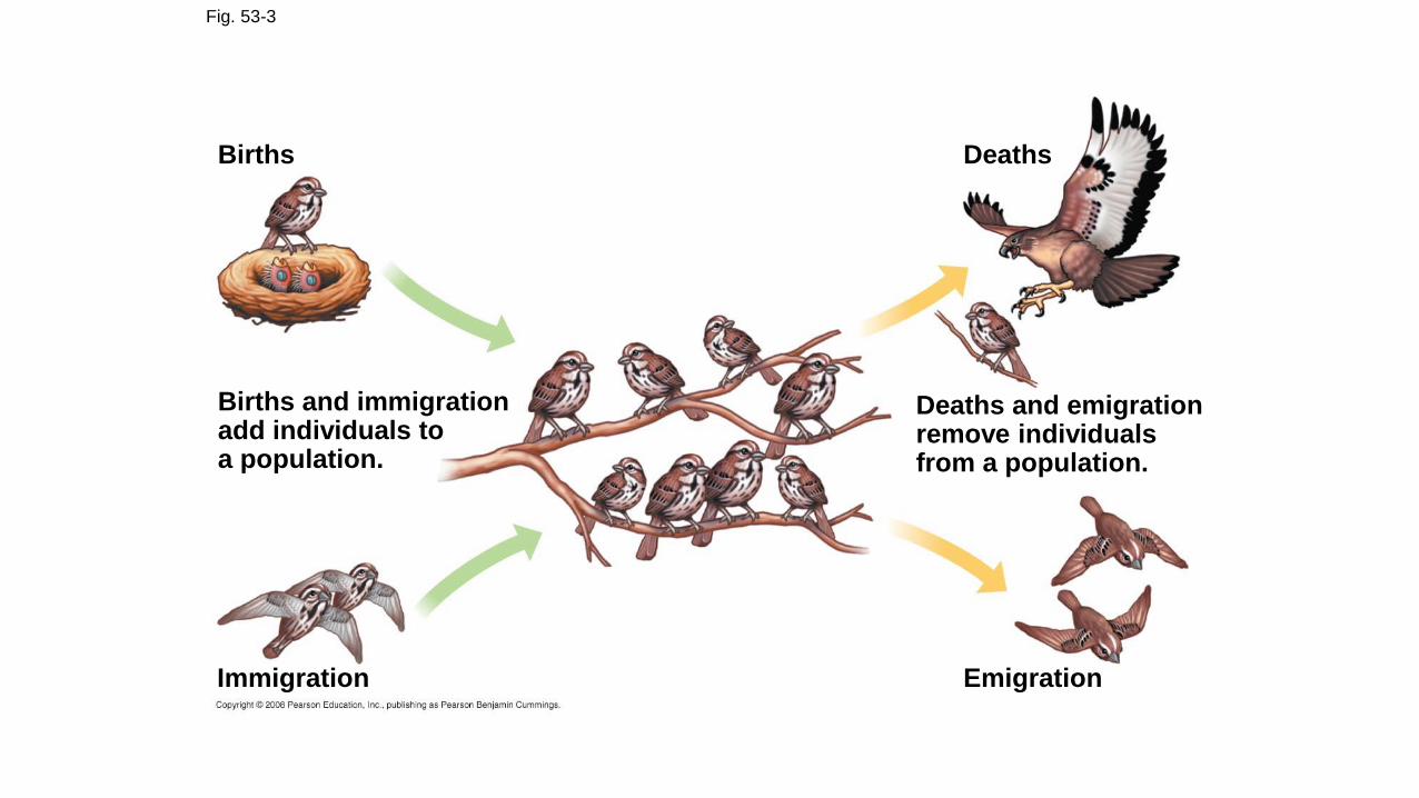
Fig. 53-3

Births

Births and immigrationadd individuals toa population.

Immigration

Deaths and emigrationremove individualsfrom a population.

Deaths

Emigration

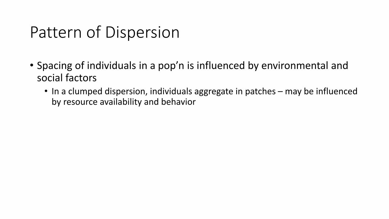
Pattern of Dispersion

• Spacing of individuals in a pop’n is influenced by environmental and social factors• In a clumped dispersion, individuals aggregate in patches – may be influenced

by resource availability and behavior

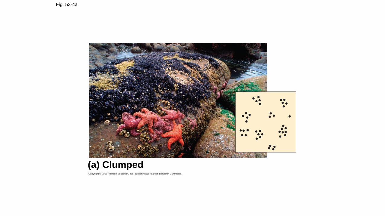
Fig. 53-4a

(a) Clumped

• Uniform dispersion – evenly distributed• Influenced by social interactions such as territoriality

• Random dispersion – position is independent of other individuals• Occurs in the absence of strong attractions or repulsions

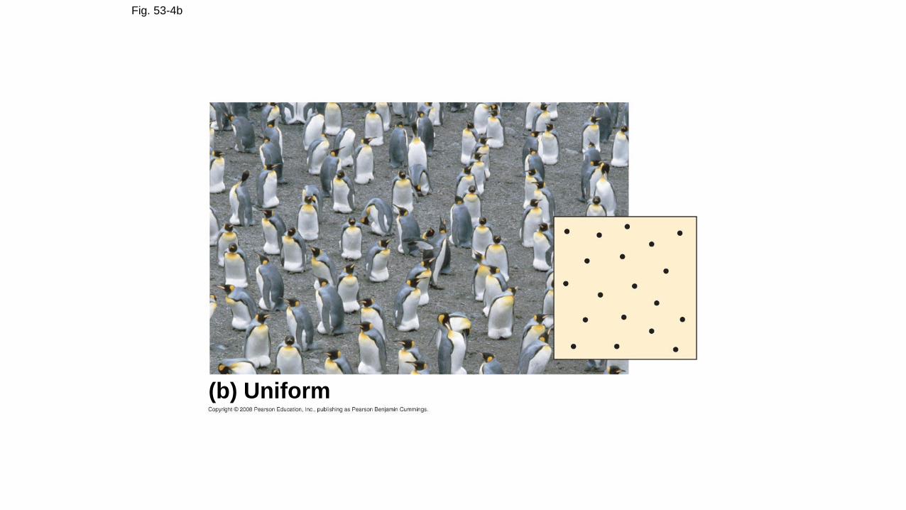
Fig. 53-4b

(b) Uniform

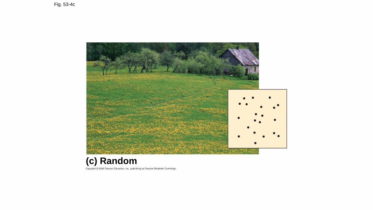
Fig. 53-4c

(c) Random

Demography and Life Tables

• Study of vital statistics of a population and how they change over time

• Death and birth rates – interest demographers

• Life table – age specific summary of the survival pattern of a pop’n

• Follow a cohort (group of individuals of same age)

Table 53-1

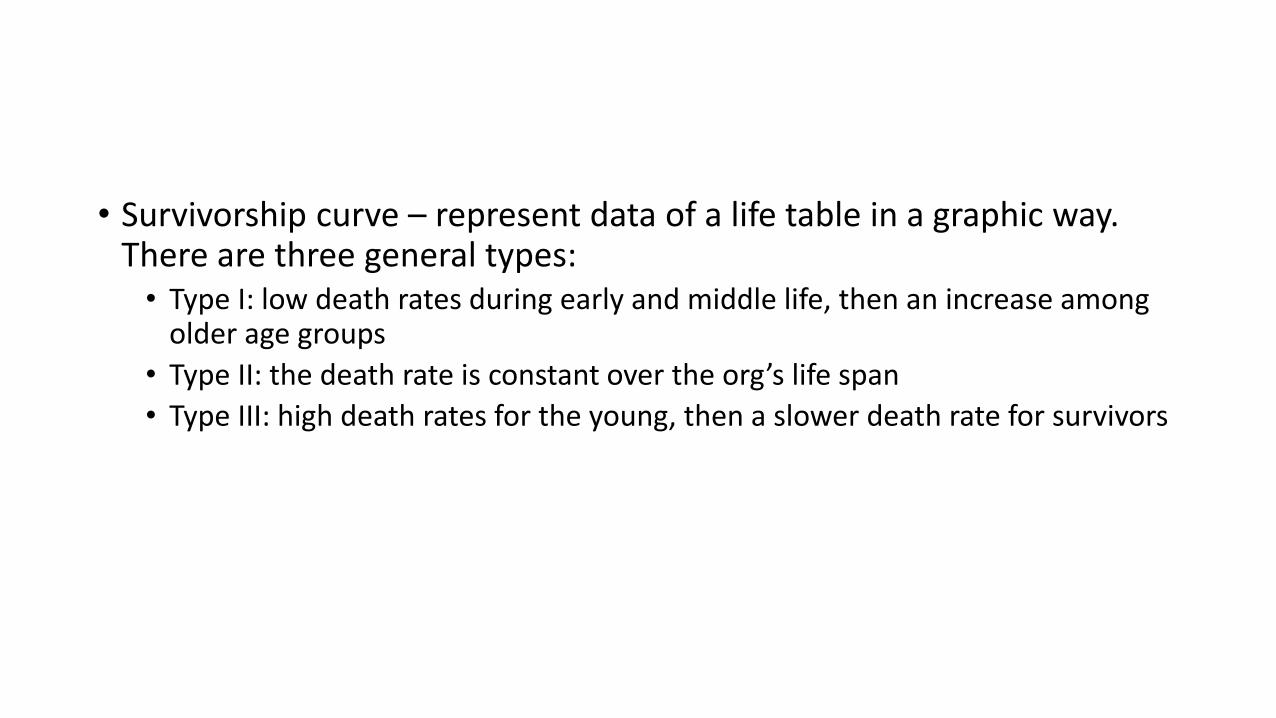
• Survivorship curve – represent data of a life table in a graphic way. There are three general types:• Type I: low death rates during early and middle life, then an increase among

older age groups

• Type II: the death rate is constant over the org’s life span

• Type III: high death rates for the young, then a slower death rate for survivors

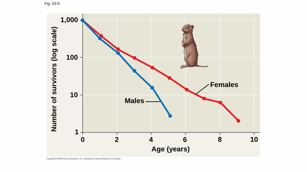
Fig. 53-5

Age (years)

20 4 86

10

101

1,000

100N

um

ber

of

su

rviv

ors

(lo

g s

ca

le)

Males

Females

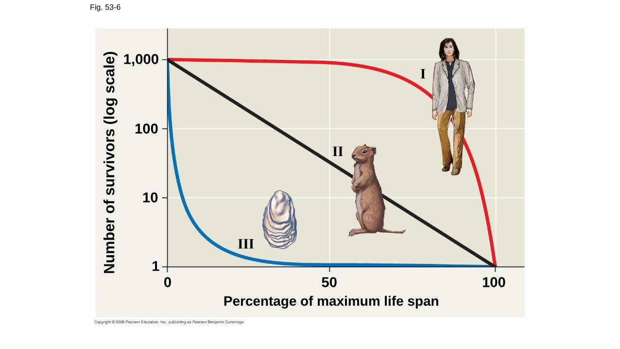
Fig. 53-6

1,000

100

10

10 50 100

II

III

Percentage of maximum life span

Nu

mb

er

of

su

rviv

ors

(lo

g s

ca

le)

I

Reproductive Rates

• For species with sexual reproduction, females used

• A reproductive table, or fertility schedule is an age-specific summary of the reproductive rates in a population

• Describes reproductive patterns of a pop’n

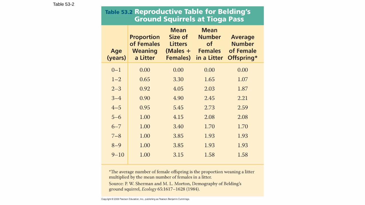
Table 53-2

• Life history of org comprises the traits that affect its schedule of reproduction and survival:• Age at which reproduction begins

• How often the organism reproduces

• How many offspring are produced during each reproductive cycle

• Life history traits are evolutionary outcomes reflected in the development, physiology, and behavior of an organism

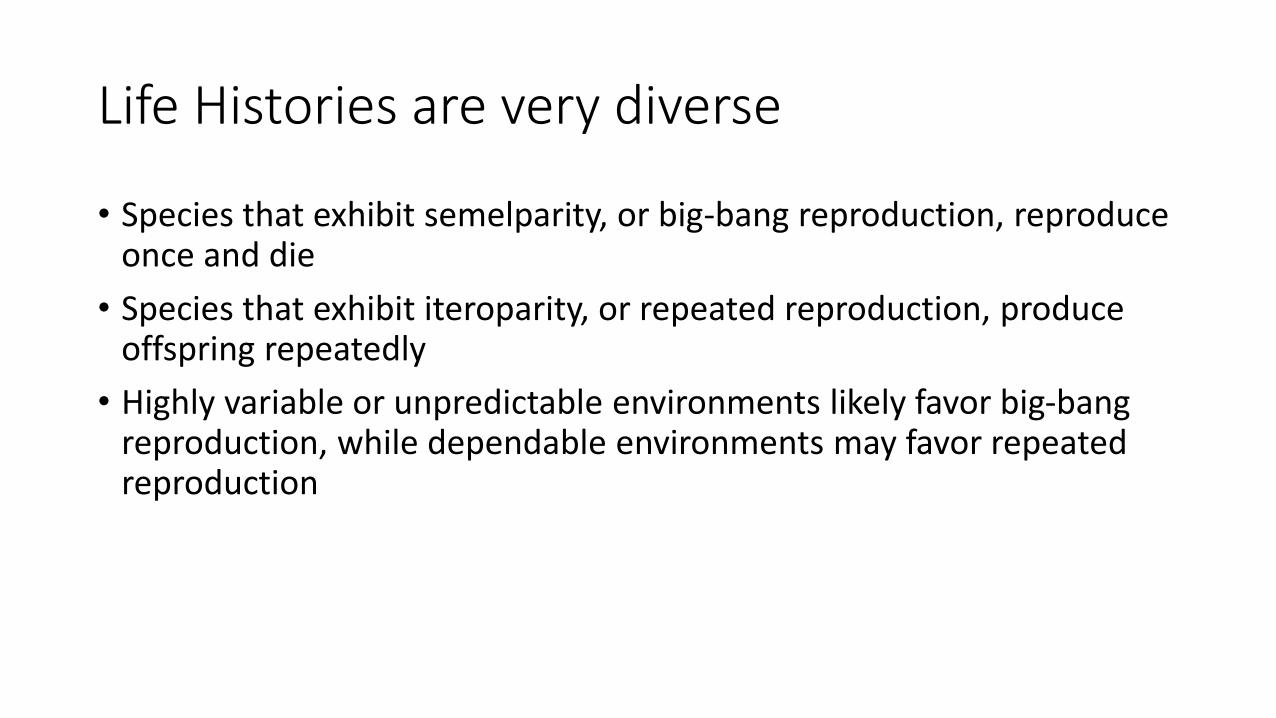
Life Histories are very diverse

• Species that exhibit semelparity, or big-bang reproduction, reproduce once and die

• Species that exhibit iteroparity, or repeated reproduction, produce offspring repeatedly

• Highly variable or unpredictable environments likely favor big-bang reproduction, while dependable environments may favor repeated reproduction

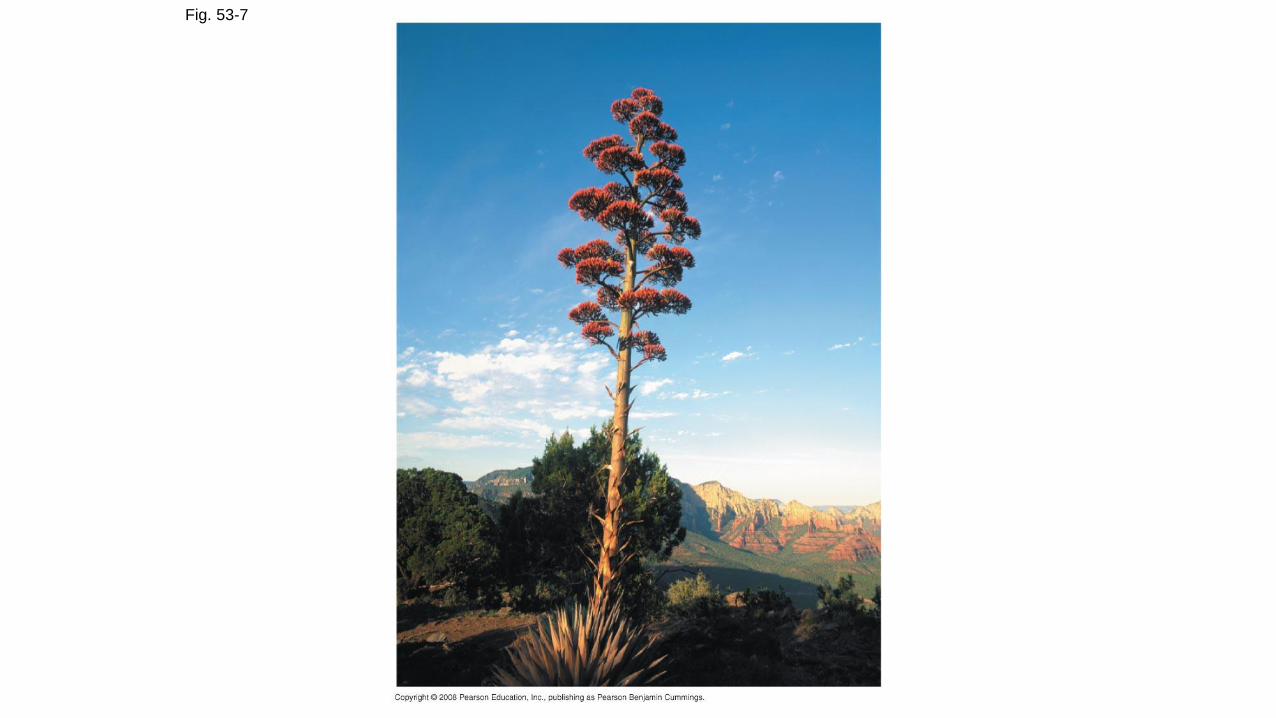
Fig. 53-7

“Trade-offs” and Life Histories

• Organisms have finite resources, which may lead to trade-offs between survival and reproduction• Some plants produce a large number of small seeds, ensuring that at least

some of them will grow and eventually reproduce

• Other types of plants produce a moderate number of large seeds that provide a large store of energy that will help seedlings become established

Fig. 53-9

(a) Dandelion

(b) Coconut palm

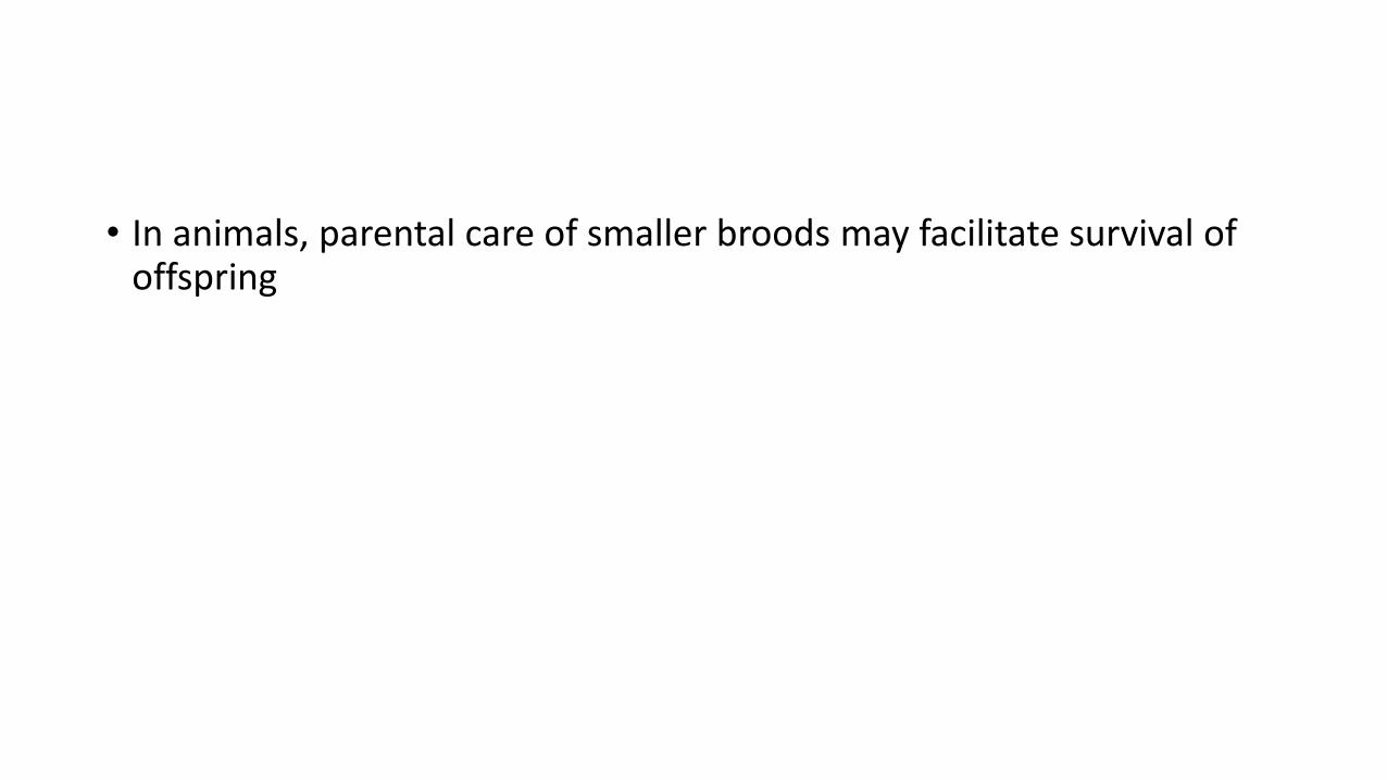
• In animals, parental care of smaller broods may facilitate survival of offspring

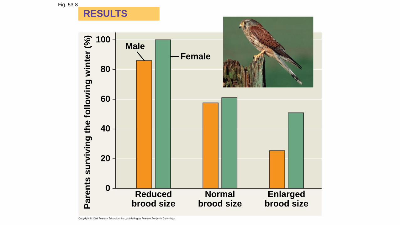
Fig. 53-8

MaleFemale

100

RESULTS

80

60

40

20

0Reduced

brood sizeNormal

brood sizeEnlarged

brood sizePare

nts

su

rviv

ing

th

e f

oll

ow

ing

win

ter

(%)

Population Growth Models

• It is useful to study pop’n growth in an idealized situation• Help us understand the capacity of a species to increase and the conditions

that may facilitate this growth

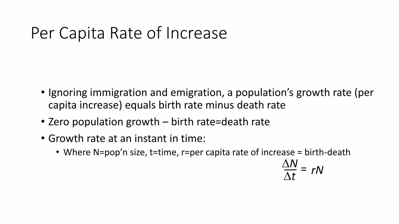
Per Capita Rate of Increase

• Ignoring immigration and emigration, a population’s growth rate (per capita increase) equals birth rate minus death rate

• Zero population growth – birth rate=death rate

• Growth rate at an instant in time:• Where N=pop’n size, t=time, r=per capita rate of increase = birth-death

Nt

= rN

Exponential population growth

• Increase under idealized conditions

• Rate of reproduction is at its max, called intrinsic rate of increase

• Eq’n of exponential pop’n growth:

• Growth results in a J-shaped curve

• J-shaped curve of exponential growth characterizes some rebounding pop’ns dN

dtrmaxN

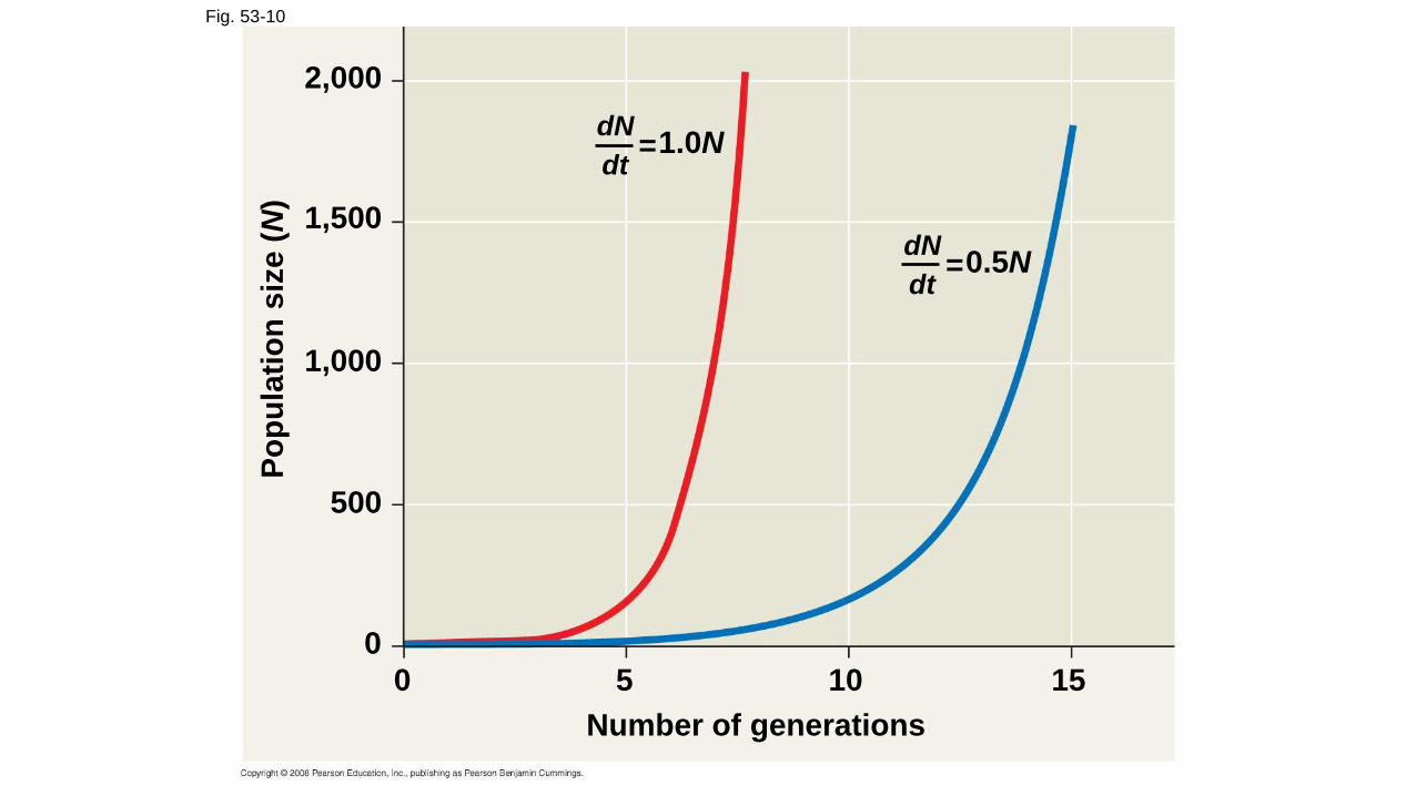
Fig. 53-10

Number of generations

0 5 10 15

0

500

1,000

1,500

2,000

1.0N=dN

dt

0.5N=dN

dtP

op

ula

tio

n s

ize (

N)

Fig. 53-11

8,000

6,000

4,000

2,000

01920 1940 1960 1980

Year

Ele

ph

an

t p

op

ula

tio

n

1900

Logistic Growth Model

• Exponential growth cannot be sustained for long in any population

• A more realistic population model limits growth by incorporating carrying capacity

• Carrying capacity(K) is the max pop’n size the enviro can support

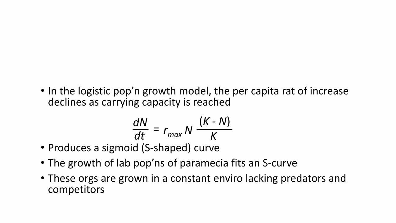
• In the logistic pop’n growth model, the per capita rat of increase declines as carrying capacity is reached

• Produces a sigmoid (S-shaped) curve

• The growth of lab pop’ns of paramecia fits an S-curve

• These orgs are grown in a constant enviro lacking predators and competitors

dNdt

=(K - N)

Krmax N

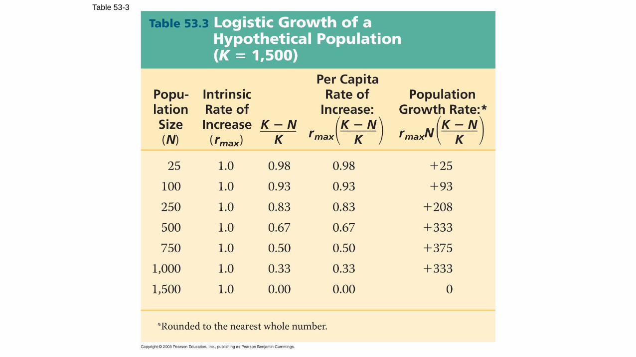
Table 53-3

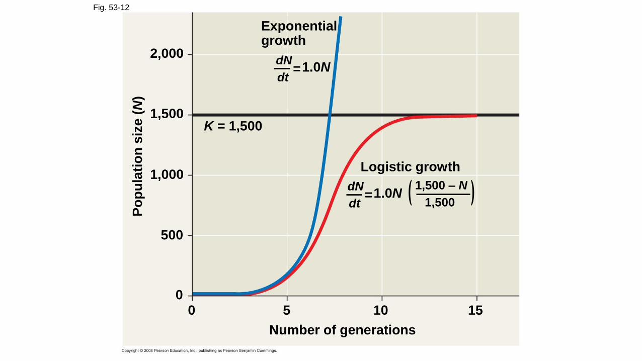
Fig. 53-12

2,000

1,500

1,000

500

00 5 10 15

Number of generations

Po

pu

lati

on

siz

e (

N)

Exponentialgrowth

1.0N=dN

dt

1.0N=dN

dt

K = 1,500

Logistic growth

1,500 – N

1,500

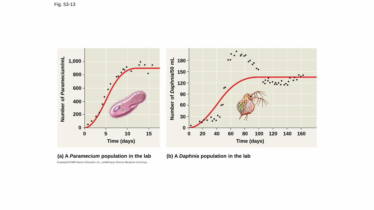
Fig. 53-13

1,000

800

600

400

200

0

0 5 10 15

Time (days)

Nu

mb

er

of

Pa

ram

ec

ium

/mL

Nu

mb

er

of

Da

ph

nia

/50 m

L

0

30

60

90

180

150

120

0 20 40 60 80 100 120 140 160

Time (days)

(b) A Daphnia population in the lab(a) A Paramecium population in the lab

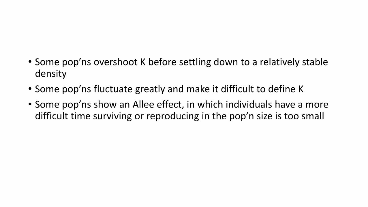
• Some pop’ns overshoot K before settling down to a relatively stable density

• Some pop’ns fluctuate greatly and make it difficult to define K

• Some pop’ns show an Allee effect, in which individuals have a more difficult time surviving or reproducing in the pop’n size is too small

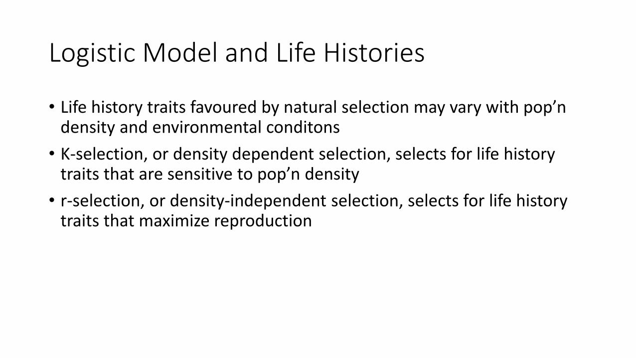
Logistic Model and Life Histories

• Life history traits favoured by natural selection may vary with pop’ndensity and environmental conditons

• K-selection, or density dependent selection, selects for life history traits that are sensitive to pop’n density

• r-selection, or density-independent selection, selects for life history traits that maximize reproduction

Density dependent factors in population growth

• General questions about regulation of pop’n growth:

• What environmental factors stop a population from growing indefinitely

• Why do some populations show radical fluctuations in size over time, while others remain stable?

• In density-independent populations, birth rate and death rate do not change with pop’n density

• In density-dependent pop’ns, birth rates fall and death rates rise with pop’n density

• Density-dependent birth and death rates are an example of negative feedback that regulates pop’n growth

• They are affected by many factors, such as competition for resources, territoriality, disease, predation, toxic wastes, and intrinsic factors

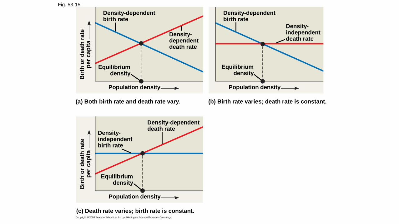
Fig. 53-15

(a) Both birth rate and death rate vary.

Population density

Density-dependentbirth rate

Equilibriumdensity

Density-dependentdeath rate

Bir

th o

r d

ea

th r

ate

per

cap

ita

(b) Birth rate varies; death rate is constant.

Population density

Density-dependentbirth rate

Equilibriumdensity

Density-independentdeath rate

(c) Death rate varies; birth rate is constant.

Population density

Density-dependentdeath rate

Equilibriumdensity

Density-independentbirth rate

Bir

th o

r d

ea

th r

ate

per

cap

ita

• In crowded populations, increasing pop’n density intensifies competition for resources and results in a lower birth rate

• In many vertebrates competition for territory may limit density

• Ex: cheetah are highly territorial, use chemical communication to warn other cheetahs of their boundaries

• Ex: oceanic birds exhibit territoriality in nesting behavior

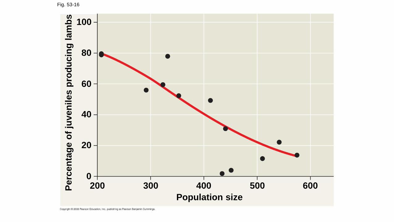
Fig. 53-16

Population size

100

80

60

40

20

0200 400 500 600300P

erc

en

tag

e o

f ju

ven

iles

pro

du

cin

g l

am

bs

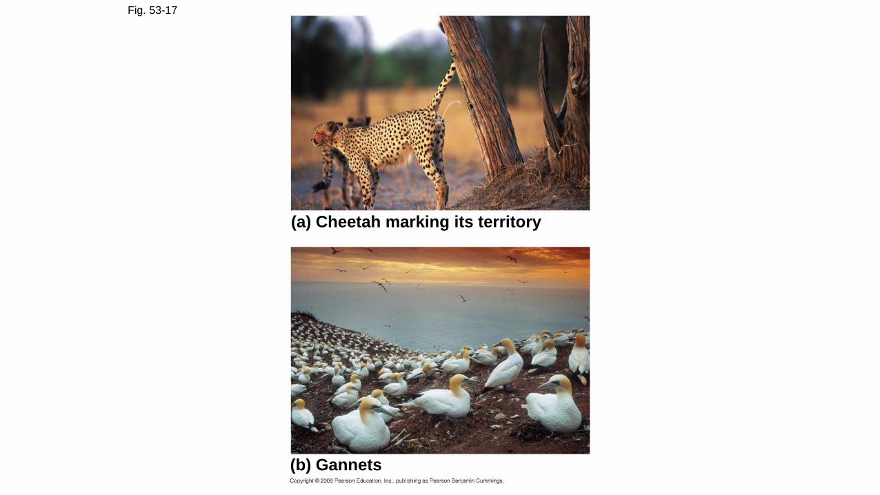
Fig. 53-17

(a) Cheetah marking its territory

(b) Gannets

• Disease• Pop’n density can influence the health and survival or organisms

• In dense pop’ns, pathogens can spread more rapidly

• Predation• As a prey pop’n build up, predators may feed preferentially on that species

• Toxic wastes - accumulation of toxic wastes can contribute to density-dependent regulation of pop’n size

• Intrinsic factors – for some pop’ns, physiological factors appear to regulate pop’n size

Population Dynamics

• Focuses on the complex interactions between biotic and abiotic factors that cause variation in pop’n size

• Weather can affect pop’n size over time

• Changes in predation pressure can drive population fluctuations

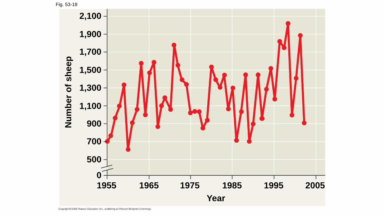
Fig. 53-18

2,100

1,900

1,700

1,500

1,300

1,100

900

700

500

01955 1965 1975 1985 1995 2005

Year

Nu

mb

er

of

sh

eep

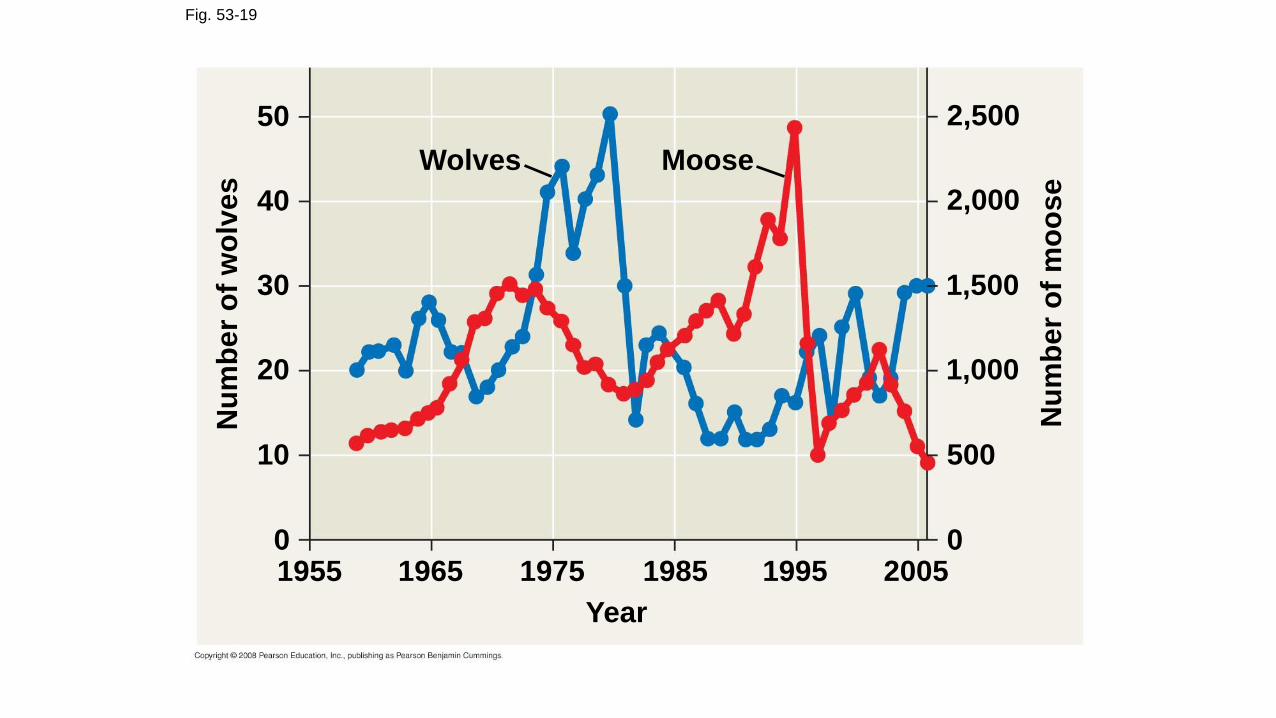
Fig. 53-19

Wolves Moose

2,500

2,000

1,500

1,000

500

Nu

mb

er

of

mo

ose

0

Nu

mb

er

of

wo

lve

s

50

40

30

20

10

01955 1965 1975 1985 1995 2005

Year

Population Cycles

• Some pop’ns undergo regular boom-and-bust cycles

• Lynx pop’ns follow the 10 year boom-and-bust cycle of hare populations

• Three hypotheses have been proposed to explain the hare’s 10-year interval

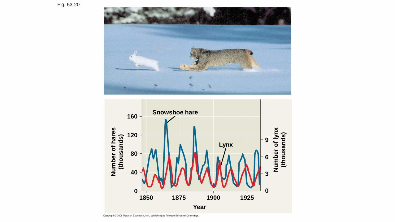
Fig. 53-20

Snowshoe hare

Lynx

Nu

mb

er

of

lyn

x

(th

ou

sa

nd

s)

Nu

mb

er

of

ha

res

(th

ou

sa

nd

s)

160

120

80

40

01850 1875 1900 1925

Year

9

6

3

0

Hypothesis: the hare’s pop’n cycle follows a cycle of winter food supply

• If this hypothesis is correct, then the cycles should stop if the food supply is increased

• Additional food was provided experimentally to a hare pop’n and the whole pop’n increased in size but continued to cycle

• No hares appeared to have died of starvation

Hypothesis: the hare’s pop’n cycle is driven by pressure from other predators

• In a field study conducted by field ecologists, 90% of the hares were killed by predatorys

• These data support this second hypothesis

Hypothesis: the hare’s pop’n cycle is linked to sunspot cycles

• Sunspot activity affects light quality, which in turn affects the quality of the hares’food

• There is good correlation between sunspot activity and hare pop’nsize

• The results of all these experiments suggest that both predation and sunspot activity regulate hare numbers and that food availability plays a less important role

Human Pop’n – exponential growth

• No pop’n can grow indefinitely, humans are no exception

• The human pop’n increased relatively slowly until about 1650 and then began to grow exponentially

• Though the global pop’n is still growing, the rate of growth began to slow during the 1960s

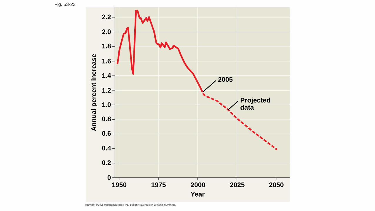
Fig. 53-23

2005

Projecteddata

An

nu

al

pe

rce

nt

inc

rea

se

Year

1950 1975 2000 2025 2050

2.2

2.0

1.8

1.6

1.4

1.2

1.0

0.8

0.6

0.4

0.2

0

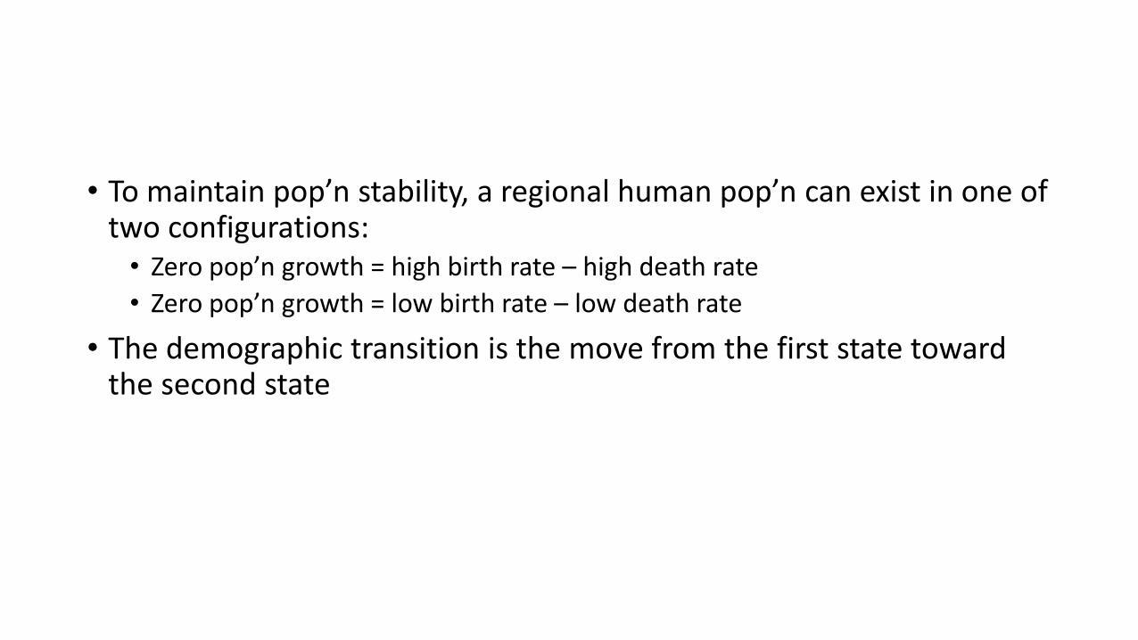
• To maintain pop’n stability, a regional human pop’n can exist in one of two configurations:• Zero pop’n growth = high birth rate – high death rate

• Zero pop’n growth = low birth rate – low death rate

• The demographic transition is the move from the first state toward the second state

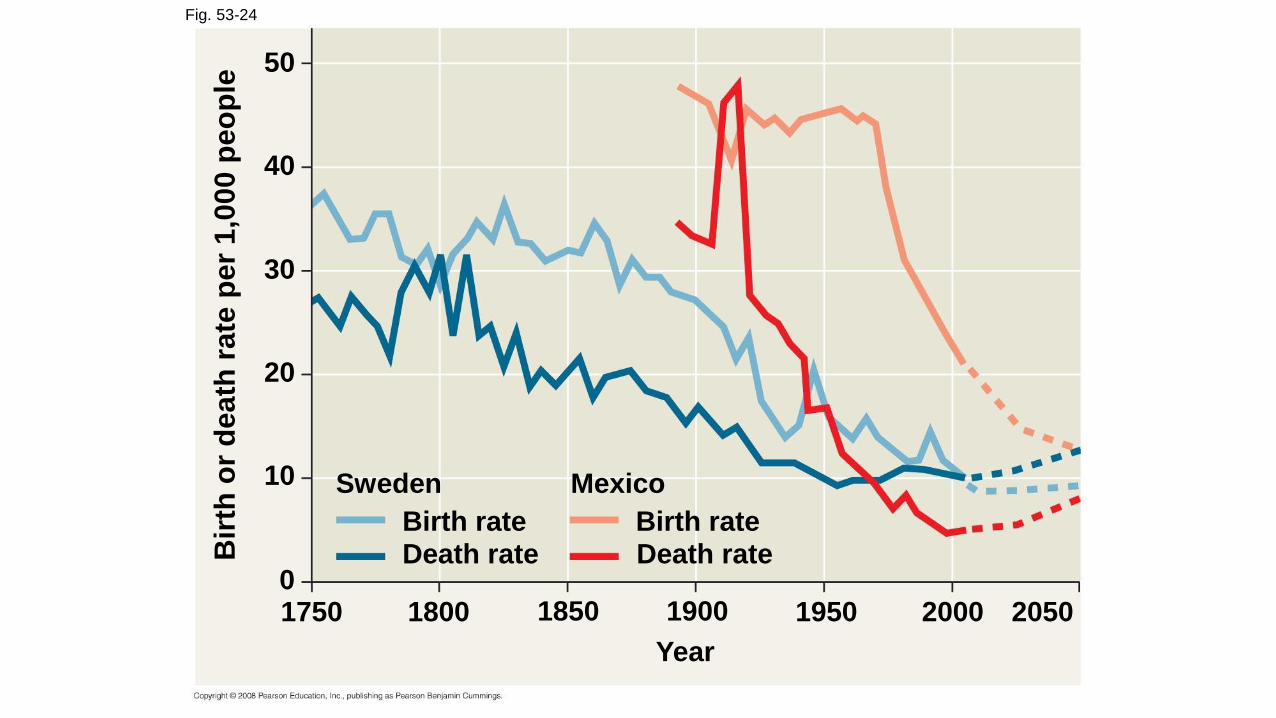
Fig. 53-24

1750 1800 1900 1950 2000 2050

Year

1850

Sweden Mexico

Birth rate Birth rateDeath rateDeath rate

0

10

20

30

40

50

Bir

th o

r d

ea

th r

ate

per

1,0

00 p

eo

ple

• The demographic transition is associated with an increase in the quality of health care and improved access to education, especially for women

• Most of the current global pop’n growth is concentrated in developing countries

Global Carrying Capacity

• How many humans can the biosphere support?

• The carrying capacity of Earth for humans is uncertain

• The average estimate is 10-15 billion

Limits on Human Population Size

• The ecological footprint concept summarizes the aggregate land and water area needed to sustain the people of a nation

• It is one measure of how close we are to the carrying capacity of Earth

• Countries vary greatly in footprint size and available ecological capacity

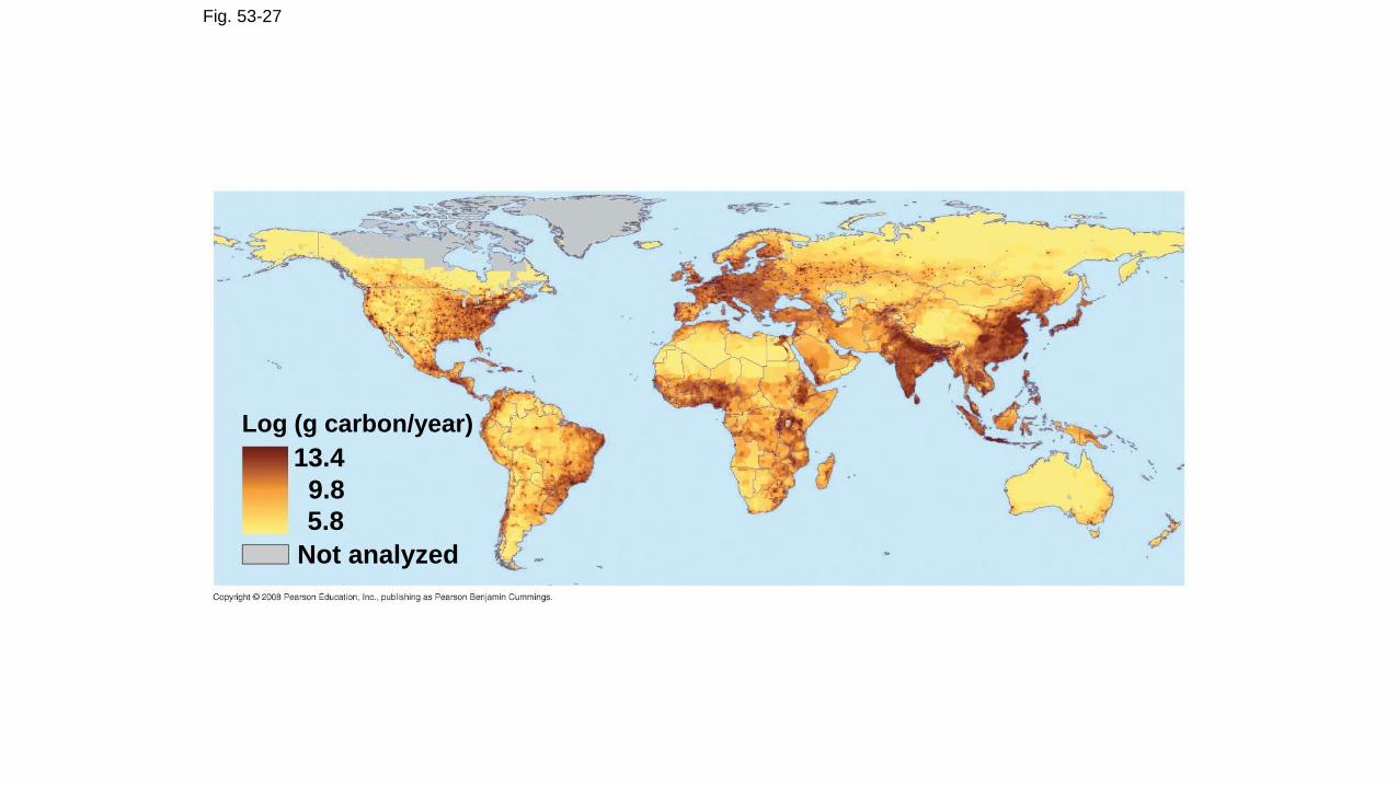
Fig. 53-27

Log (g carbon/year)

13.4

9.8

5.8

Not analyzed

• Our carrying capacity could potentially be limited by food, space, non-renewable resources, or buildup of wastes

• An ecosystem consists of all of the organisms living in a community, as well as the abiotic factors with which they interact

• Ecosystems range from a microcosm, such as an aquarium, to a large area such as a lake or forest

• Regardless of an ecosystem’s size, its dynamics involve two main processes: energy flow and chemical cycling

• Energy flows through ecosystems while matter cycles within them

• Laws of physics and chemistry apply to ecosystems, particularly energy flow

• The first law of thermodynamics states that energy cannot be created or destroyed, only transformed

• Energy enters an ecosystem as solar radiation, is conserved, and is lost from organisms as heat

• The second law of thermodynamics states that every exchange of energy increases the entropy of the universe

• In an ecosystem, energy conversion are not completely efficient, and some energy is always lost as heat

• The law of conservation of mass states that matter cannot be created or destroyed

• Chemical elements are continually recycled within ecosystems

• In a forest ecosystem, most nutrients enter as dust or solutes in rain and are carried away in water

• Ecosystems are open systems, absorbing energy and mass and releasing heat and waste products

Energy, Mass and Trophic Levels

• Autotrophs build molecules themselves using photosynthesis as an energy source; heterotrophs depend on the output of other organisms

• Energy and nutrients pass from primary producers to primary consumers (herbivores) to secondary consumers (carnivores) to tertiary consumers (carnivores that feed on other carnivores)

• Detritivores, or decomposers, are consumers that derive their energy from detritus, nonliving organic matter

• Prokaryotes and fungi are important detritivores

• Decomposition connects all trophic levels

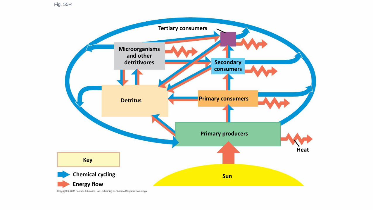
Fig. 55-4

Microorganismsand other

detritivores

Tertiary consumers

Secondaryconsumers

Primary consumers

Primary producers

Detritus

Heat

SunChemical cycling

Key

Energy flow

• Primary production in an ecosystem is the amount of light energy converted to chemical energy by autotrophs during a given time period

• The extent of photosynthetic production sets the spending limit for an ecosystem’s energy budget

Energy transfer between trophic levels is typically only 10% efficient• Secondary production of an ecosystem is the amount of chemical

energy in food converted to new biomass during a given period of time

• When a caterpillar feeds on a leaf, only about 1/6 of the leaf’s energy is used for secondary production

• An organism’s production efficiency is the fraction of energy stored in food that is not used for respiration

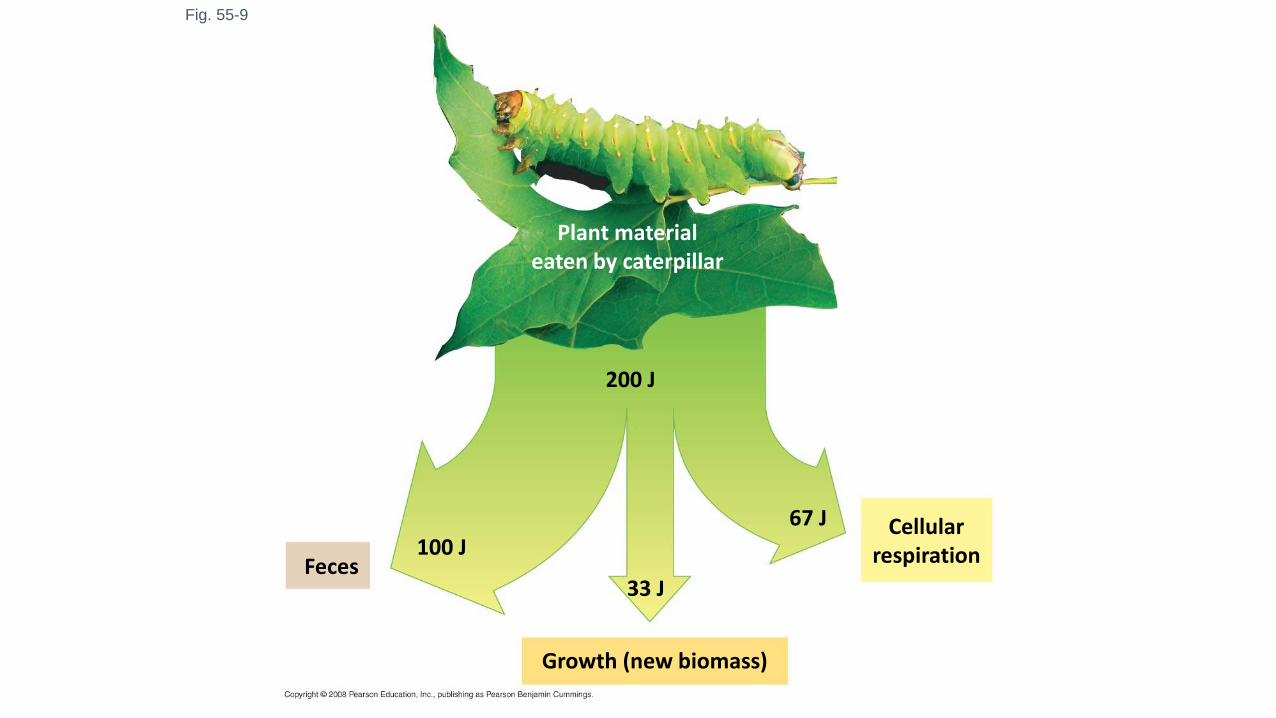
Fig. 55-9

Cellularrespiration100 J

Growth (new biomass)

Feces

200 J

33 J

67 J

Plant materialeaten by caterpillar

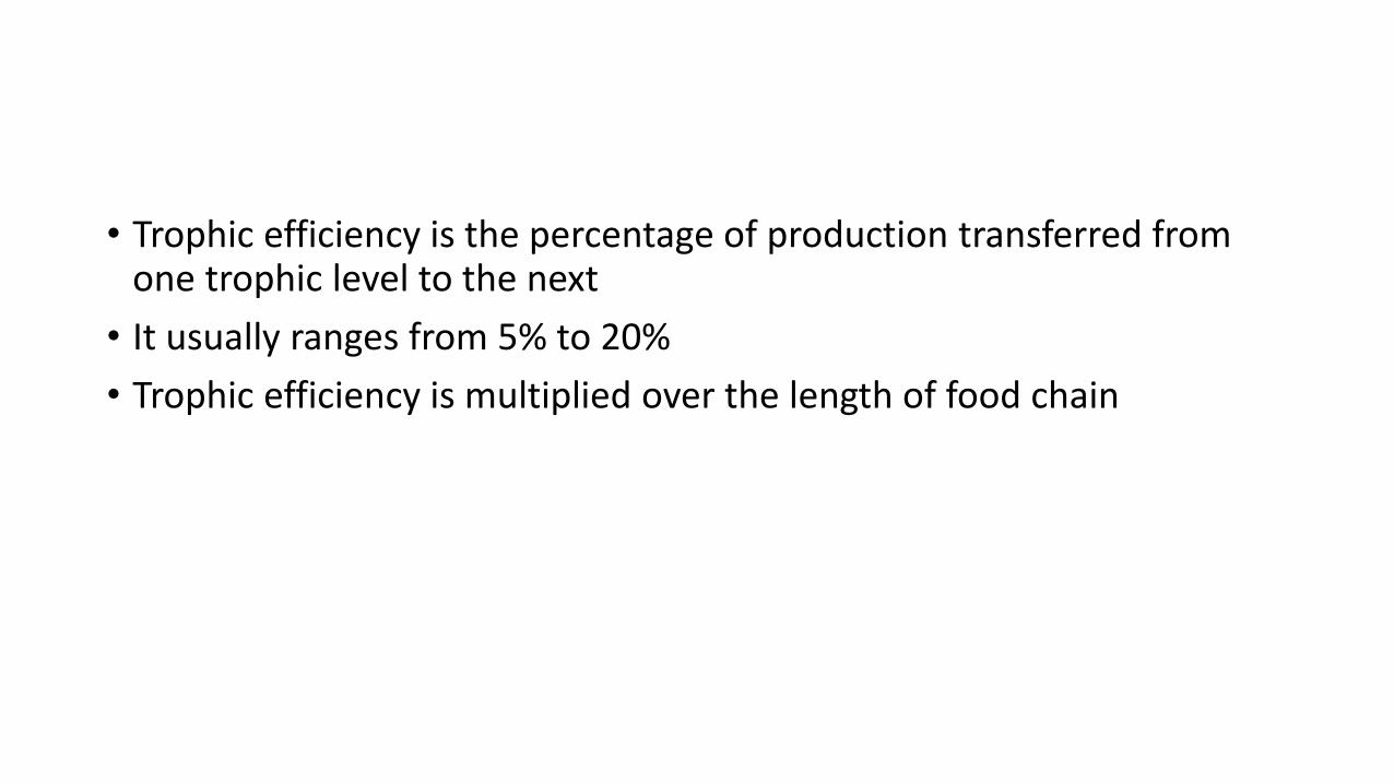
• Trophic efficiency is the percentage of production transferred from one trophic level to the next

• It usually ranges from 5% to 20%

• Trophic efficiency is multiplied over the length of food chain

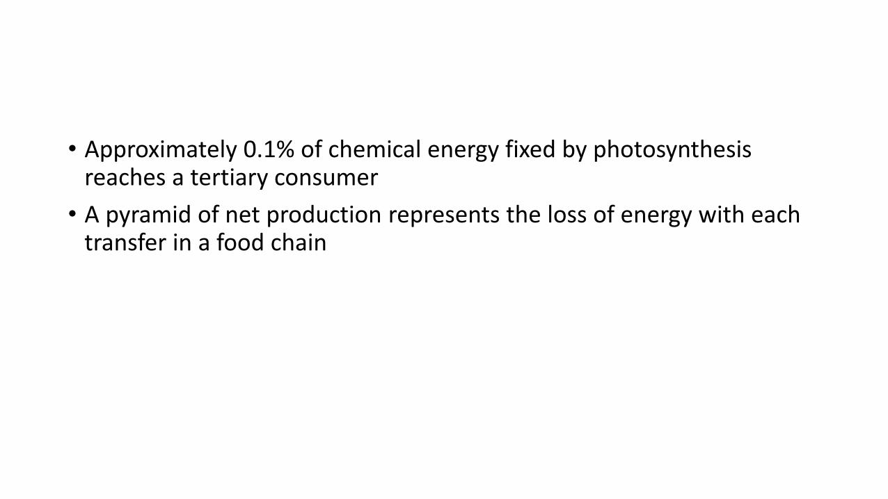
• Approximately 0.1% of chemical energy fixed by photosynthesis reaches a tertiary consumer

• A pyramid of net production represents the loss of energy with each transfer in a food chain

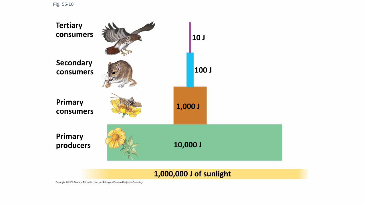
Fig. 55-10

Primaryproducers

100 J

1,000,000 J of sunlight

10 J

1,000 J

10,000 J

Primaryconsumers

Secondaryconsumers

Tertiaryconsumers

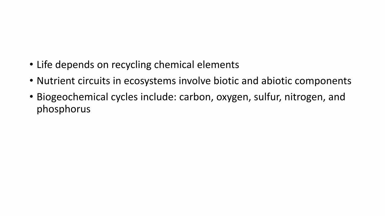
• Life depends on recycling chemical elements

• Nutrient circuits in ecosystems involve biotic and abiotic components

• Biogeochemical cycles include: carbon, oxygen, sulfur, nitrogen, and phosphorus

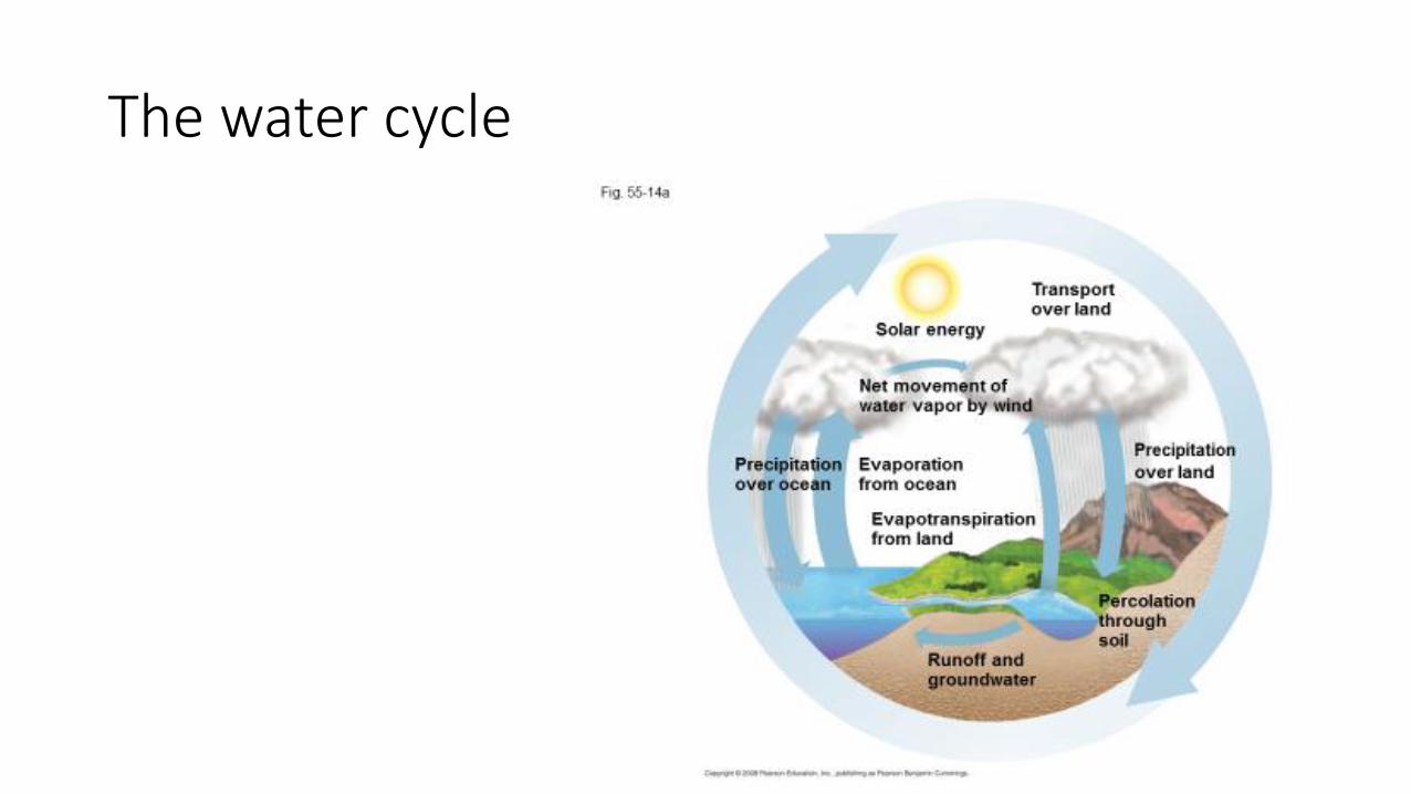
The water cycle

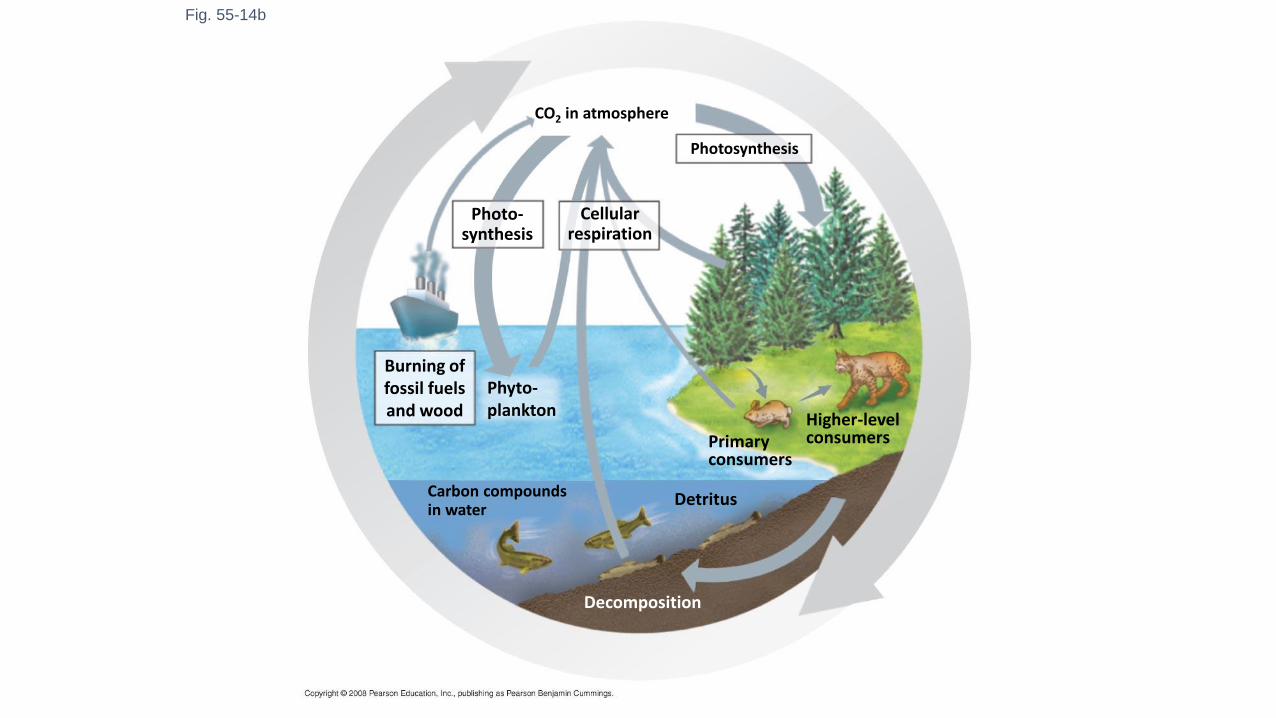
Fig. 55-14b

Higher-levelconsumersPrimary

consumers

Detritus

Burning offossil fuelsand wood

Phyto-plankton

Cellularrespiration

Photo-synthesis

Photosynthesis

Carbon compoundsin water

Decomposition

CO2 in atmosphere

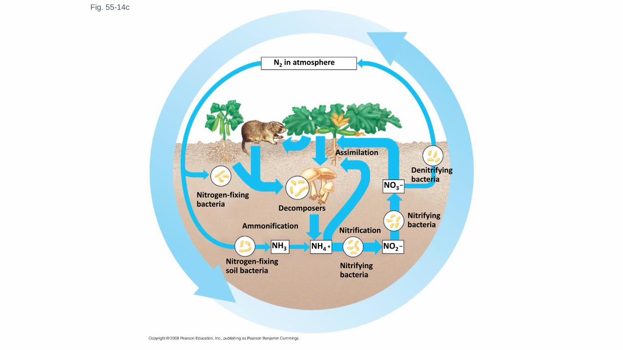
Fig. 55-14c

Decomposers

N2 in atmosphere

Nitrification

Nitrifyingbacteria

Nitrifyingbacteria

Denitrifyingbacteria

Assimilation

NH3 NH4 NO2

NO3

+ –

–

Ammonification

Nitrogen-fixingsoil bacteria

Nitrogen-fixingbacteria

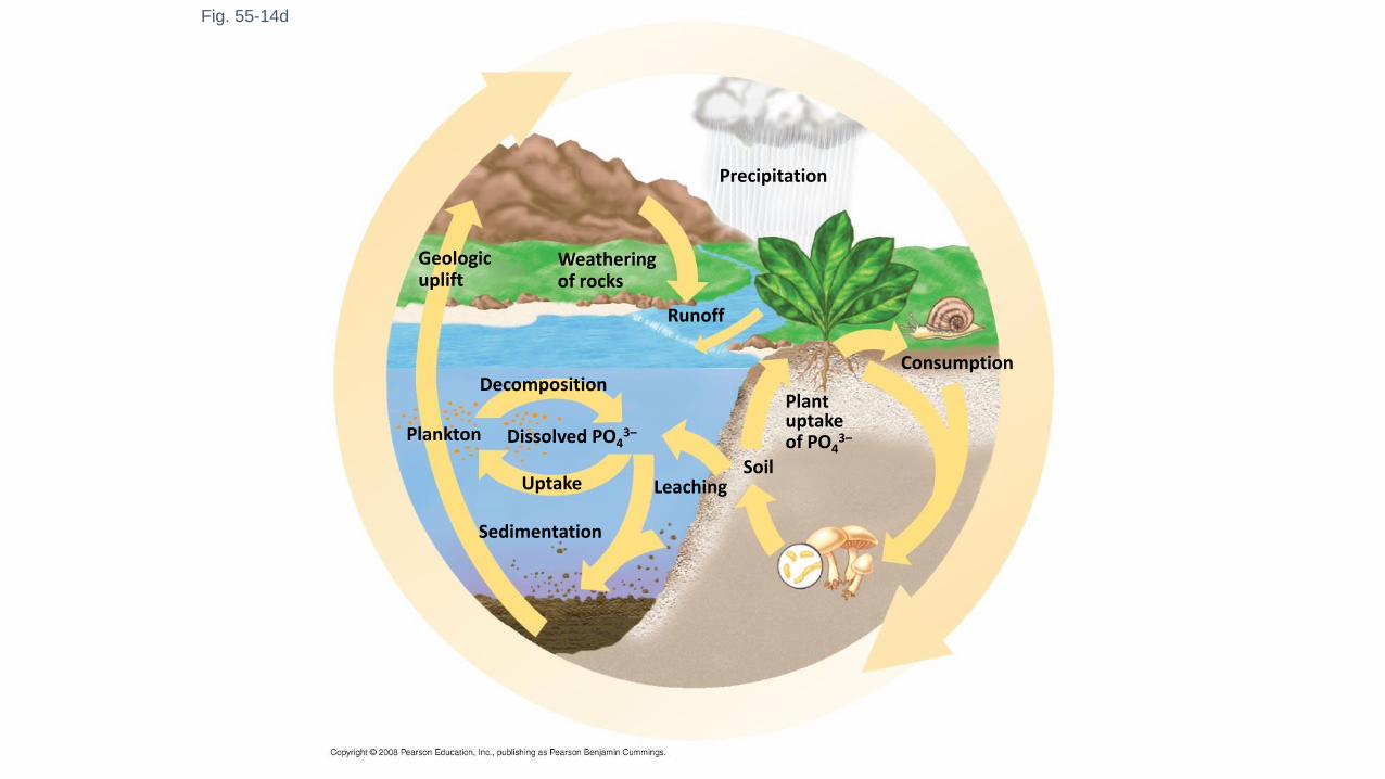
Fig. 55-14d

Leaching

Consumption

Precipitation

Plantuptakeof PO4

3–

Soil

Sedimentation

Uptake

Plankton

Decomposition

Dissolved PO43–

Runoff

Geologicuplift

Weatheringof rocks