IntroductionECON 30020: Intermediate Macroeconomics

Prof. Eric Sims

University of Notre Dame

Spring 2018

1 / 23

Readings

I GLS Chapters 1, 2, and 3

I GLS Appendix A

2 / 23

Introduction

I Macroeconomics:I Better called aggregate economicsI Focus on dynamic and intertemporal nature of economic

decision-makingI Economics is “micro”: “macro” just studies issues at

aggregated (country) level

I Key questions:I Why does the economy grow over time?I Why are some countries rich and others poor?I Why do economies experience recessions?I What is the role of government?I More recently:

I What the heck happened in 2007-2009?

3 / 23

Logistics

I SyllabusI TextbookI Assignments and gradingI Office hoursI TAsI Course outline

4 / 23

Gentle Reminder

5 / 23

About Me

I Associate Professor, Dept. of EconomicsI B.A. Trinity University, 2003

I “Miracle in Mississippi” October 27, 2007

I Ph.D. University of Michigan, 2009I Don’t get the wrong pictureI Wife proud ND graduate – Lewis chickenI Signed Charlie Weis picture in office (oops?)I Michigan Sucks

6 / 23

Out of Style

7 / 23

In Style I

8 / 23

In Style II

9 / 23

My Effect on Notre Dame Football

0

0.1

0.2

0.3

0.4

0.5

0.6

0.7

0.8

0.9

1900 1910 1920 1930 1940 1950 1960 1970 1980 1990 2000 2010

Notre Dame Winning % By Decade

ND WP

Sims arrival

10 / 23

Math

I “It is true that modern macroeconomics uses mathematicsand statistics to understand behavior in situations where thereis uncertainty about how the future will unfold from the past.But a rule of thumb is that the more dynamic, uncertain andambiguous is the economic environment that you seek tomodel, the more you are going to have to roll up your sleeves,and learn and use some math. That’s life.” – ThomasSargent, 2011 Nobel Prize Winner

11 / 23

What Kind of Math We Will Be Using

I Basically:I AlgebraI Differential calculus

I Will also need to know:I Microsoft ExcelI How to play with graphsI Some basic statistics

I See GLS Appendixes A and B

I TA office hour sessions this week

12 / 23

Variable Types and Timing Notation

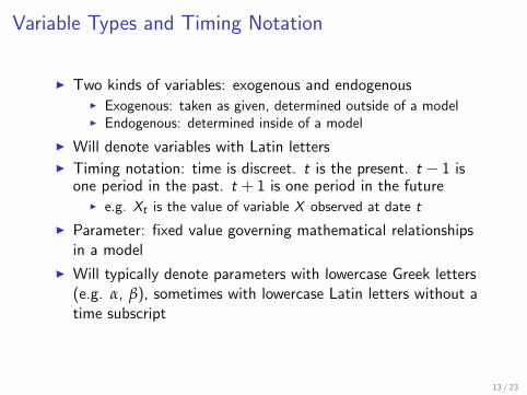
I Two kinds of variables: exogenous and endogenousI Exogenous: taken as given, determined outside of a modelI Endogenous: determined inside of a model

I Will denote variables with Latin lettersI Timing notation: time is discreet. t is the present. t − 1 is

one period in the past. t + 1 is one period in the futureI e.g. Xt is the value of variable X observed at date t

I Parameter: fixed value governing mathematical relationshipsin a model

I Will typically denote parameters with lowercase Greek letters(e.g. α, β), sometimes with lowercase Latin letters without atime subscript

13 / 23

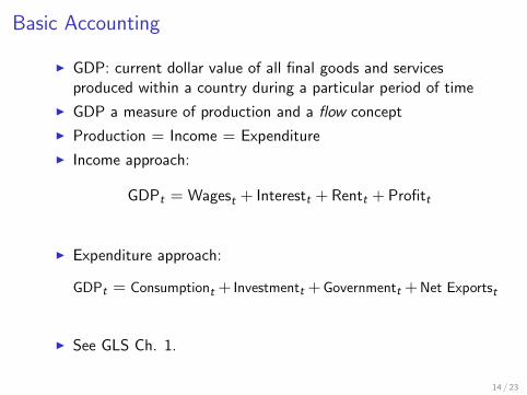
Basic Accounting

I GDP: current dollar value of all final goods and servicesproduced within a country during a particular period of time

I GDP a measure of production and a flow concept

I Production = Income = Expenditure

I Income approach:

GDPt = Wagest + Interestt + Rentt + Profitt

I Expenditure approach:

GDPt = Consumptiont + Investmentt +Governmentt +Net Exportst

I See GLS Ch. 1.

14 / 23

Real vs. Nominal I

I GDP is defined in terms of current dollar prices

I Effectively, prices are weights reflecting relative valuations ofdifferent goods

I But makes comparisons across time difficult

I Want a “real” or “inflation-adjusted” measure of GDP

I How to do this?

15 / 23

Real vs. Nominal II

I In a single good world (most of this course), something real isdenominated in quantities of goods, whereas nominal ismeasured in units of money (i.e. dollars)

I So suppose you produce 10 cans of beer valued at $2 per can.Real quantity is 10 cans, nominal value is $20

I Not so obvious how to do this with many different goods (thereal world, but not most of this course)

I Solution: “constant dollar” GDP. Value quantities of goods atdifferent points in time using fixed prices (base year prices).So real GDP actually denominated in units of money, butfacilitates comparisons over time

I Can “back out” a measure of aggregate prices via the implicitprice index: ratio of nominal (current dollar) GDP to real(constant dollar) GDP

I Inflation: rate of growth of price index

16 / 23

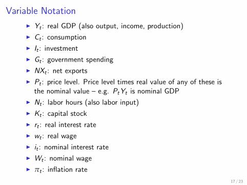
Variable Notation

I Yt : real GDP (also output, income, production)

I Ct : consumption

I It : investment

I Gt : government spending

I NXt : net exports

I Pt : price level. Price level times real value of any of these isthe nominal value – e.g. PtYt is nominal GDP

I Nt : labor hours (also labor input)

I Kt : capital stock

I rt : real interest rate

I wt : real wage

I it : nominal interest rate

I Wt : nominal wage

I πt : inflation rate

17 / 23

What Economists Do

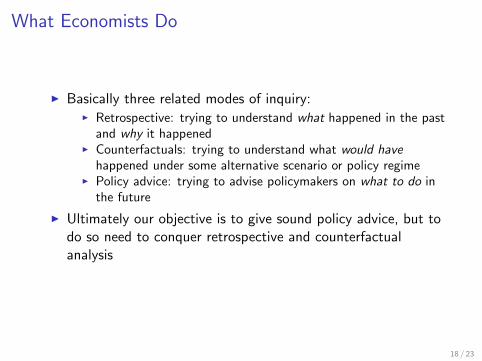
I Basically three related modes of inquiry:I Retrospective: trying to understand what happened in the past

and why it happenedI Counterfactuals: trying to understand what would have

happened under some alternative scenario or policy regimeI Policy advice: trying to advise policymakers on what to do in

the future

I Ultimately our objective is to give sound policy advice, but todo so need to conquer retrospective and counterfactualanalysis

18 / 23

Models

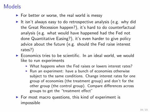
I For better or worse, the real world is messy

I It isn’t always easy to do retrospective analysis (e.g. why didthe Great Recession happen?), it’s hard to do counterfactualanalysis (e.g. what would have happened had the Fed notdone Quantitative Easing?), it’s even harder to give policyadvice about the future (e.g. should the Fed raise interestrates?)

I Economics tries to be scientific. In an ideal world, we wouldlike to run experiments

I What happens when the Fed raises or lowers interest rates?I Run an experiment: have a bunch of economies otherwise

subject to the same conditions. Change interest rates for onegroup of economies (the treatment group) and don’t for theother group (the control group). Compare differences acrossgroups to get the “treatment effect”

I For most macro questions, this kind of experiment isimpossible

19 / 23

The Art and Science of Economic Models

I Because experiments aren’t in play, economists use models

I Given a model, we try do “real science”: run experiments, anduse the outcomes from those experiments to inform policy

I But building the model itself is as much art as it is science

20 / 23

A Model

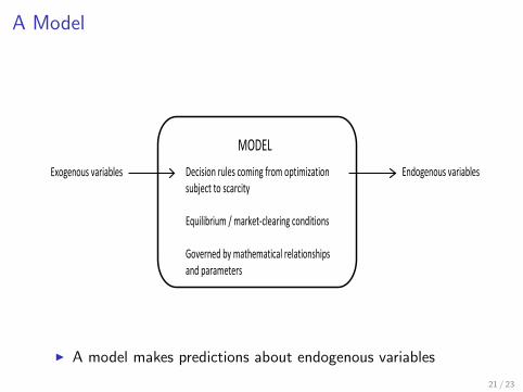
Decision rules coming from optimization subject to scarcity Equilibrium / market-clearing conditions Governed by mathematical relationships and parameters

MODEL Exogenous variables Endogenous variables

I A model makes predictions about endogenous variables

21 / 23

How to Judge / Build a Model

I No firm criteria. This is the “art” partI Characteristics of a good model:

I Makes good predictionsI Stronger test: makes good predictions about things which it

wasn’t designed to explain (“over-identification”)

I Is as simple as possibleI Abstract from things which are not relevantI The simpler it is, the easier it is to understand the mechanisms

I Makes reasonable assumptions

22 / 23

Models in This Course

I In macro, we do a lot of abstraction (e.g. we assume everyoneis the same!)

I Course divided into three “runs” which feature differing levelsof abstraction:

I Long run (decades): abstract from endogenous labor input andmany sources of shocks, focus on capital accumulation andproductivity growth. Solow model

I Medium run (several years): abstract from capitalaccumulation and productivity growth, abstract from nominalprice and wage rigidity. Neoclassical model

I Short run (months to several years): abstract from capitalaccumulation and productivity growth, allow for price and/orwage stickiness. New Keynesian model

I In addition, close the course with a section on banking/financeand the Great Recession, which builds off the short run part

23 / 23