Introduction - isip.piconepress.com€¦ · Web viewThe problem that we are trying to solve is to predict the performance of a search term especially for spoken-term-detection (STD)

111Equation Chapter 1 Section 1

Keyword Search Assessment

Internal Report

By: Amir Harati and Joseph Picone

[email protected], [email protected]

ISIP, Department of Electrical Engineering, Temple University

Jan 2012

1. Introduction

This project is continuation of “Spoken-Term-Detection” term assessment project1. In the current project, BBN2 database is used (NIST and BBN used previously). This project has several goals:

1. Test a new approach based on acoustic distance measure to predict error rate of a given word.2. Try some new machines/features to predict error rates.3. Combine different machines optimally to increase the predictive capabilities

Because of some different settings we decided to rewrite most of the code. The only things that imported from previous project are BBN data (which has been extracted from raw data provided by BBN.), duration model (extracted from TIMIT database) and phonetic distance based models. Everything else, including predictor machines, is rewritten for consistency issues.

This report can be divided into 9 parts. The second part introduces the problem and a brief review of approaches used in this work. The third section introduce Spoken term detection task briefly. The fourth part introduces data. In this section we introduce the BBN database and also we introduce the way we divided this data into train-evaluation sections. The fifth part introduces acoustic-distance based methods. The sixth part is about phonetic-distance based method. Again results are explained. The seventh part is presenting features based methods. In this section we introduce features used in this project. Especially a new feature (in respect to previous work) that we have used and its relevance would be discussed. We also talk about different feature selection methods that used and finally results of different feature based predictors are presented. In section eight, we discuss about combining all these different machines using a particle swarm optimization (PSO) based algorithm.

mailto:[email protected]

2. Problem

The problem that we are trying to solve is to predict the performance of a search term especially for spoken-term-detection (STD) systems. The error rate of a word depends on various factors but generally we can say it is related to its confusability and acoustical and phonetical properties. Moreover, there are some other factors unrelated to the word itself that influence its error rate. Among them are the environmental noise, accent, speech rate, and context. These additional factors make the problem of error rate prediction somewhat difficult since in our setting the only thing that we are given is the word and not the additional factors (which can be assumed uncontrolled and lumped into general noise factor.)

We have used three general approaches to solve this problem: One approach is based on direct use of acoustic data. The major assumption for this approach is that acoustic similarities between different words are generally related to their error rate. Words with similar acoustic units are expected to perform similarly in speech recognizer. Another approach is based on phonetic similarities. Again the assumption is that words with similar phonetic structure should perform similarly against a speech recognizer. The third approach is based on several features extracted from words. In this approach we assume that these features represent the underlying reasons that affect the error rates of a word.

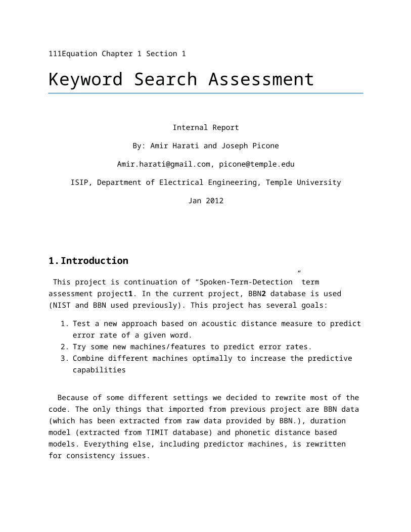
All in all, the problem is converted to a regression problem, in which the error rate is the variable of interest. Figure 1 shows the overall system architecture.

3. Spoken Term Detection

Spoken term detection (STD) systems differ from text search engines in one significant manner – the match between a keyword and the audio data is approximate and is typically based on a likelihood computed from some sort of pattern recognition system. The performance of such systems depends on many external factors such as the acoustic channel, speech rate, accent, language, and the confusability of search terms. In this work, our focus is on the latter issue. Our goal is to develop algorithms to predict the reliability or strength of a search term using the error rate of the system as measure of the performance.

The accuracy of a search term is a critical issue for frequent users of this technology. Unlike text searches, sorting through audio data that has been incorrectly matched can be a time consuming and frustrating process. State of the art systems based on this technology produce results that are not always intuitive. Therefore, the goal of this work is provide users some prior knowledge of which search terms are likely to be more accurate than others. Password strength checkers, which are a similar technology, have become very commonplace, and represent a functional model for this work.

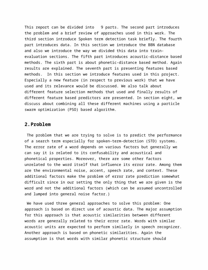
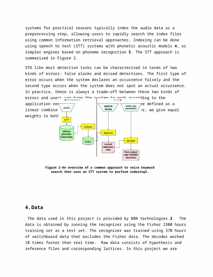
The goal of a typical STD system 3 is “to rapidly detect the presence of a term in large audio corpus of heterogeneous speech material.” STD systems for practical reasons typically index the audio data as a preprocessing step, allowing users to rapidly search the index files using common information retrieval

Figure 1-System Architecture

approaches. Indexing can be done using speech to text (STT) systems with phonetic acoustic models 4, or simpler engines based on phoneme recognition 5. The STT approach is summarized in Figure 2.

STD like most detection tasks can be characterized in terms of two kinds of errors: false alarms and missed detections. The first type of error occurs when the system declares an occurrence falsely and the second type occurs when the system does not spot an actual occurrence. In practice, there is always a trade-off between these two kinds of errors and users can tune the system to work according to the application requirements. The overall error could be defined as a linear combination of these two terms. In this paper, we give equal weights to both factors.

4. Data

The data used in this project is provided by BBN technologies 2. The data is obtained by running the recognizer using the Fisher 2300 hours training set as a test set. The recognizer was trained using 370 hours of switchboard data that excludes the Fisher data. The decoder worked 10 times faster than real time. Raw data consists of hypothesis and reference files and corresponding lattices. In this project we are interested to extract error rate related to each word. This can be accomplished by comparing hypothesis and reference file using dynamic programming techniques. Alternatively, we can use sctk program provided by NIST 6. However, since the file sizes are very big we finally decided to write our own scoring program to calculate error rates. We can also compute the average duration of each word using lattices provided with the data. This duration information is used to compare with result of our duration model that will be discussed later. Details of procedures and all related codes can be found under “data_extraction” directory.

4.1 Generating Training and Evaluation Subsets

In order to evaluate algorithms meaningfully we should have completely separate sets for training and evaluation. However, dividing the data into two parts and using one part for evaluation and one for training is a wasteful approach, especially by considering the fact that the amount of available data is limited. Another option is to use cross-validation. In this approach we divide the whole data set into N (in this case 10) subsection and at each step use one of these subsections as the evaluation set and other 9

Figure 2-An overview of a common approach to voice keyword search that uses an STT system to perform indexing3.

subsets as training data. At each step we should train our models completely from scratch and using the corresponding training data. After completing this step for all 10 subsets we can concatenate the results to obtain the evaluation results for all data point. Statistics for training (MSE, correlation and R-Square) can be obtained by averaging these statistics for individual training set. Because of the reasons that will be explained later (see section 8) each training subset divided into 10 subsets (dev sets) so we can calculate the prediction of each algorithm just over each training data set using a similar paradigm that we have used to calculate the prediction over the evaluation sets.

Since data, for different algorithms, is different (for example for acoustic based method data is the representation vectors and for feature based method data is a collection of features.) , we first divide labels into 10 sections and then using this fixed labels divide the data for different algorithms.

5. Acoustic Distance Based Algorithm

One intuitive way to predict the error rate associated to a word is to look at similar words and deduce the error rate of the word in question by averaging (or weighted averaging) of those similar words. Depending on the criterion used to define the similarity, many different algorithms can be obtained. In this section we describe an algorithm that is based on acoustical similarities between words. In the next section we will introduce an algorithm based on phonetical similarities.

5.1 Data Preparation

Acoustic data can be extracted from various sources. In this project we have used Switch board (SWB) dataset 7. The method is very simple.

First a list of words existed in our dataset is generated. Then all instances of these words are spotted in the transcriptions and corresponding MFCC files. This step is possible because transcriptions at word level are available.

Because different words and even different instances of the same word have different lengths and at the other hand, we want to generate vectors with equal length we use a simple procedure to convert all instances of all words into vectors with predefined length. Toward this we have used three approaches and correspondingly produced three sets of data.

The first method is adopted from 8. In this method each utterance is segmented into three sections with relative size 3-4-3 and the average value is calculated in each segment as a result we obtain a 3*39 =117 elements vector, now we add the log of the duration for that utterance to obtain a final vector with length 118. The second method is similar to the first method but we have segmented the utterance into segments with relative size of 10-24-32-24-10.Finally for the last method utterance is segmented into 10 equal segments.

There exists many examples for each word. As a result we have to use some method to briefly represent each word. In other words we want to represent a word by just few vectors. One approach, which we have used in this work, is based on K-mean clustering. By changing K we can segment the data for each word

into several regions and use the center of each region as a representative for that word. This can be thought as a simple vector quantization like approach.

5.2 Algorithm

The algorithm is a modified version of K-nearest neighbor (KNN) algorithm.

1. First all representative vectors for a given word are retrieved.

2. All of these vectors are compared with all of the vectors in the database (which excludes the word under consideration.)

3. K nearest neighbors for each representative vector and their corresponding distances are retrieved.

4. Based on the distances, the best representative vector for the word under the question is selected.

5. Weighted average of the error rates corresponding to all K selected vectors is reported as the prediction for the error rate for the word in question.

In this algorithm K can be infinite which practically means all points in the database are used to calculate the prediction but their effect is proportional to their Euclidean distances to the word in question.

5.3 Results

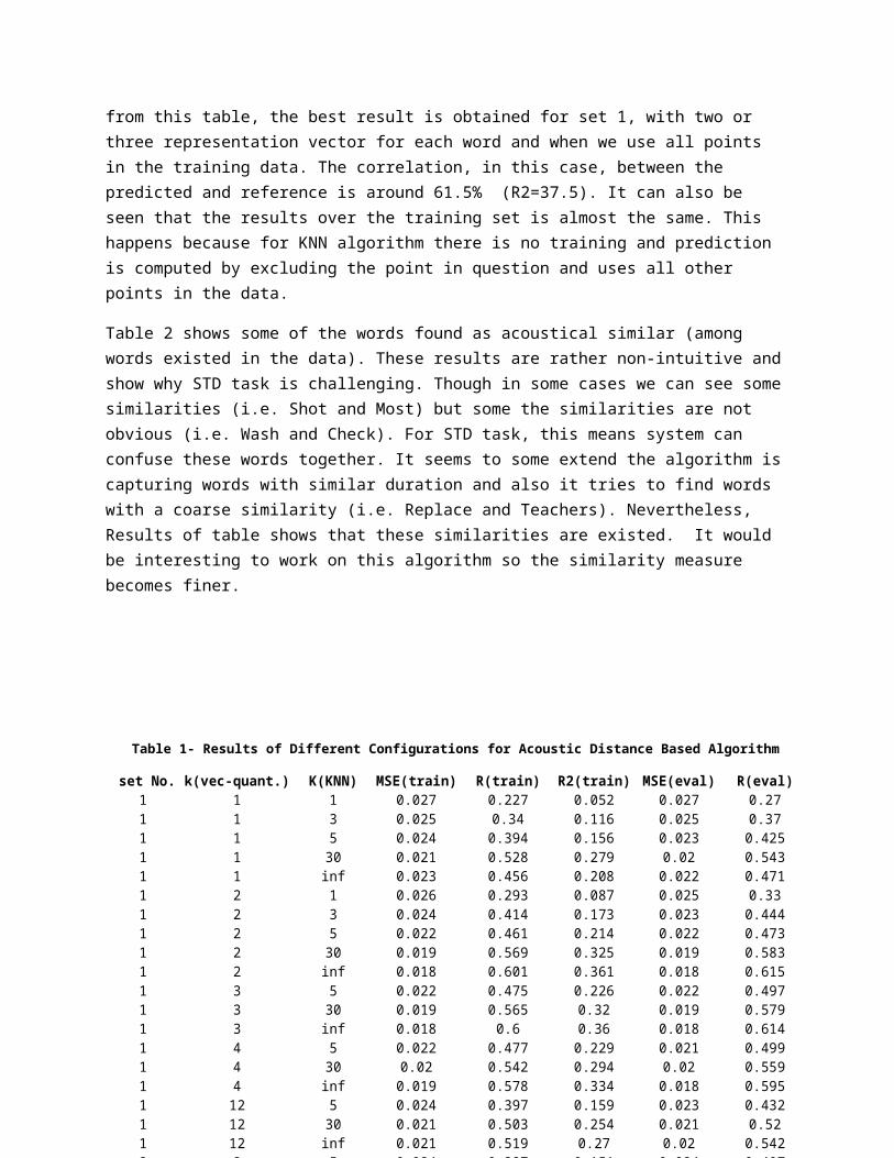
Table 1 shows the result of this algorithm for different configurations. In this table “set No.” is the data set used. (Corresponding to data sets produced in section 5.1). “k (vec-quant)” is representing the number of vectors used to represent each word. “K (KNN)” is the K for KNN algorithm. “inf” means to use all points in the training data set. The next three columns are MSE, correlation and R-Square for the training data and the last three columns are MSE, correlation and R-Square for the evaluation data. As it is evident from this table, the best result is obtained for set 1, with two or three representation vector for each word and when we use all points in the training data. The correlation, in this case, between the predicted and reference is around 61.5% (R2=37.5). It can also be seen that the results over the training set is almost the same. This happens because for KNN algorithm there is no training and prediction is computed by excluding the point in question and uses all other points in the data.

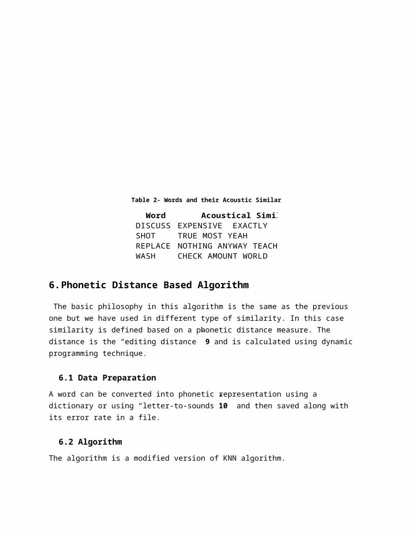
Table 2 shows some of the words found as acoustical similar (among words existed in the data). These results are rather non-intuitive and show why STD task is challenging. Though in some cases we can see some similarities (i.e. Shot and Most) but some the similarities are not obvious (i.e. Wash and Check). For STD task, this means system can confuse these words together. It seems to some extend the algorithm is capturing words with similar duration and also it tries to find words with a coarse similarity (i.e. Replace and Teachers). Nevertheless, Results of table shows that these similarities are existed. It would be interesting to work on this algorithm so the similarity measure becomes finer.

6. Phonetic Distance Based Algorithm

The basic philosophy in this algorithm is the same as the previous one but we have used in different type of similarity. In this case similarity is defined based on a phonetic distance measure. The distance is the “editing distance” 9 and is calculated using dynamic programming technique.

Table 1- Results of Different Configurations for Acoustic Distance Based Algorithm

set No. k(vec-quant.) K(KNN) MSE(train) R(train) R2(train) MSE(eval) R(eval) R2(eval) 1 1 1 0.027 0.227 0.052 0.027 0.27 0.0731 1 3 0.025 0.34 0.116 0.025 0.37 0.1371 1 5 0.024 0.394 0.156 0.023 0.425 0.1811 1 30 0.021 0.528 0.279 0.02 0.543 0.2961 1 inf 0.023 0.456 0.208 0.022 0.471 0.2221 2 1 0.026 0.293 0.087 0.025 0.33 0.1091 2 3 0.024 0.414 0.173 0.023 0.444 0.1981 2 5 0.022 0.461 0.214 0.022 0.473 0.2241 2 30 0.019 0.569 0.325 0.019 0.583 0.341 2 inf 0.018 0.601 0.361 0.018 0.615 0.3781 3 5 0.022 0.475 0.226 0.022 0.497 0.2471 3 30 0.019 0.565 0.32 0.019 0.579 0.3361 3 inf 0.018 0.6 0.36 0.018 0.614 0.3781 4 5 0.022 0.477 0.229 0.021 0.499 0.2491 4 30 0.02 0.542 0.294 0.02 0.559 0.3131 4 inf 0.019 0.578 0.334 0.018 0.595 0.3551 12 5 0.024 0.397 0.159 0.023 0.432 0.1871 12 30 0.021 0.503 0.254 0.021 0.52 0.2711 12 inf 0.021 0.519 0.27 0.02 0.542 0.2942 2 5 0.024 0.387 0.151 0.024 0.407 0.1662 4 inf 0.02 0.55 0.303 0.019 0.568 0.3232 15 inf 0.021 0.526 0.277 0.02 0.551 0.3032 17 inf 0.021 0.526 0.277 0.02 0.551 0.3033 2 inf 0.022 0.478 0.229 0.022 0.495 0.2463 2 inf 0.022 0.478 0.229 0.022 0.495 0.246

Table 2- Words and their Acoustic Similar

Word Acoustical SimilarDISCUSS EXPENSIVE EXACTLY PERCENTSHOT TRUE MOST YEAHREPLACE NOTHING ANYWAY TEACHERSWASH CHECK AMOUNT WORLD


A word can be converted into phonetic representation using a dictionary or using “letter-to-sounds”10 and then saved along with its error rate in a file.

6.2 Algorithm

The algorithm is a modified version of KNN algorithm.

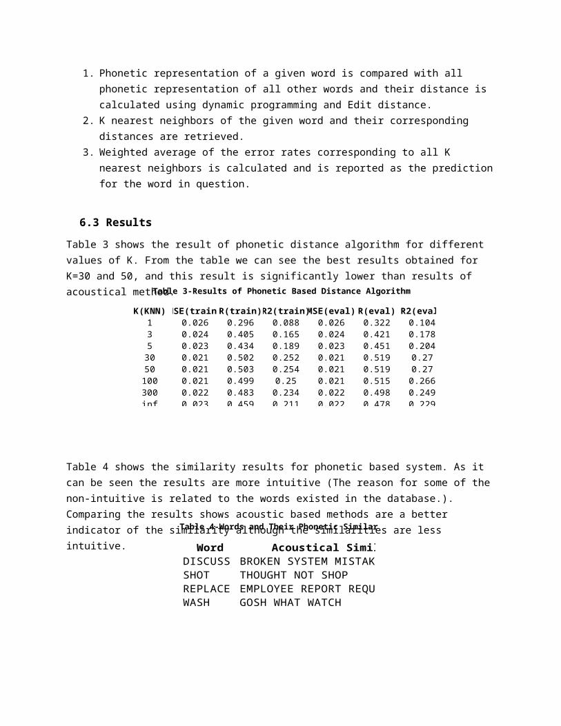
1. Phonetic representation of a given word is compared with all phonetic representation of all other words and their distance is calculated using dynamic programming and Edit distance.

2. K nearest neighbors of the given word and their corresponding distances are retrieved. 3. Weighted average of the error rates corresponding to all K nearest neighbors is calculated and is

reported as the prediction for the word in question.

6.3 Results

Table 3 shows the result of phonetic distance algorithm for different values of K. From the table we can see the best results obtained for K=30 and 50, and this result is significantly lower than results of acoustical method.

Table 4 shows the similarity results for phonetic based system. As it can be seen the results are more intuitive (The reason for some of the non-intuitive is related to the words existed in the database.). Comparing the results shows acoustic based methods are a better indicator of the similarity although the similarities are less intuitive.

Table 3-Results of Phonetic Based Distance Algorithm

K(KNN) MSE(train) R(train) R2(train) MSE(eval) R(eval) R2(eval) 1 0.026 0.296 0.088 0.026 0.322 0.1043 0.024 0.405 0.165 0.024 0.421 0.1785 0.023 0.434 0.189 0.023 0.451 0.204

30 0.021 0.502 0.252 0.021 0.519 0.2750 0.021 0.503 0.254 0.021 0.519 0.27

100 0.021 0.499 0.25 0.021 0.515 0.266300 0.022 0.483 0.234 0.022 0.498 0.249 inf 0.023 0.459 0.211 0.022 0.478 0.229

Table 4-Words and Their Phonetic Similar

Word Acoustical SimilarDISCUSS BROKEN SYSTEM MISTAKESHOT THOUGHT NOT SHOPREPLACE EMPLOYEE REPORT REQUIREWASH GOSH WHAT WATCH

7. Feature Based Algorithms

The last two algorithms were based on finding similar words in the database and estimate the error rate of the word in question by averaging the error rate of these similar words. In this section, we introduce several algorithms based on features extracted from words. Algorithms used in this section are standard machine learning algorithms and their basic feature set is the same. These algorithms include linear regression, neural network, regression tree and random forest.


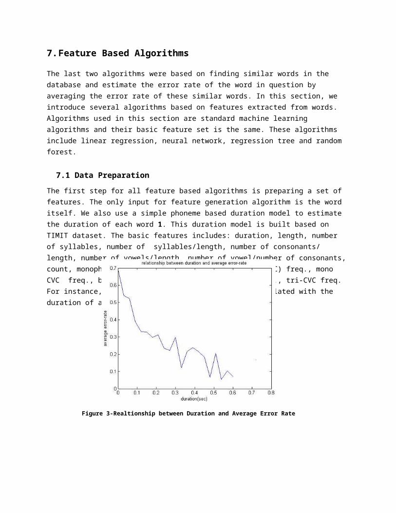
The first step for all feature based algorithms is preparing a set of features. The only input for feature generation algorithm is the word itself. We also use a simple phoneme based duration model to estimate the duration of each word 1. This duration model is built based on TIMIT dataset. The basic features includes: duration, length, number of syllables, number of syllables/length, number of consonants/ length, number of vowels/length, number of vowel/number of consonants, count, monophone freq., mono broad phonetic class (BPC) freq., mono CVC freq., bi-phone freq., bi-BPC freq. ,bi-CVC freq., tri-CVC freq. For instance, Figure 3 shows that error rate is correlated with the duration of a word.

Number of syllables can be inferred from a dictionary or alternatively using software similar to NIST syllabification 11. Consonants, vowels and their ratios can be deduced using phonetic representation of a word. Count is the number of times a word existed in the dataset. The reason that count has some information about the error rate can be explained by considering the fact that error rate is related to the number of instances of a word that recognizer is trained with. Because count is a relative measure we can infer it from an independent dataset or even using language modeling resources. However in the current work we have used BBN data to deduce the count. BPC are broad phonetic classes as shown in Table 5. CVC are consonant-vowel-consonants sequences. The frequency measures simply show the fraction of

Figure 3-Realtionship between Duration and Average Error Rate

Table 5- Broad Phonetic Class

Stops b p d t g kFricatives jh ch sh s z zh f th v dh hhNasals m n ng en Liquids l el r w yVowels iy ih eh ey ae aa aw ay ah ao ax oy ow uh iw erSilence sp sil

times each symbol (in N-gram sense) happened in a given word. After generating these basic features and also after deleting all features that never occurred or occurred very rarely we run several feature selection algorithm that are discussed in the next section.

7.2 Feature Selection

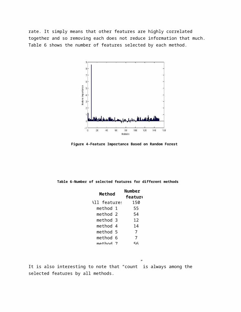
Several algorithms have been used to generate subsets of features. Before applying any algorithm we have 150 features (subset0). Subsets 1 to 6 are generated using sequential feature selection algorithm 12 with different criterion functions. Subsets 1 and 2 are generated using linear regression and using correlation and MSE respectively. Subsets 3 and 4 are using neural networks and subsets 5 and 6 are generated using trees and bagging (10 trees). Subset 7 is generated using random forest13. Figure 4 shows the feature importance according to random forest. Interestingly, count is recognized as the most important feature (its removal cause the highest increase in error.) It does not mean that it is the most correlated feature to the error rate. It simply means that other features are highly correlated together and so removing each does not reduce information that much. Table 6 shows the number of features selected by each method.

Figure 4-Feature Importance Based on Random Forest

Table 5- Broad Phonetic Class

Stops b p d t g kFricatives jh ch sh s z zh f th v dh hhNasals m n ng en Liquids l el r w yVowels iy ih eh ey ae aa aw ay ah ao ax oy ow uh iw erSilence sp sil

Table 6-Number of selected features for different methods

Method

All features 150method 1 55method 2 54method 3 12method 4 14method 5 7method 6 7

Number of features

It is also interesting to note that “count” is always among the selected features by all methods.

7.3 Algorithms

7.3.1 Linear RegressionLinear regression is among the simplest methods that can be used to model some observations. Equation 2 and 3 shows the model and training respectively. Where we want to learn β and ε is the error term.

22\* MERGEFORMAT ()

33\* MERGEFORMAT ()

7.3.2 Feed-forward Neural NetworkFeed-forward networks are among the most efficient ways to model nonlinear relationship between the inputs and the output. In this case we simply try to estimate function f in equation 4. In practice, f is approximated as a weighed sum of some simple functions like logistic or sigmoid functions and the goal is to learn these weights. The training can be accomplished using the famous back-propagation algorithm14.

44\* MERGEFORMAT ()

7.3.3 Regression TreeRegression tree is based on the intuition that in complex problems it might be beneficial to first partition the space into several homogenous subspaces (where interaction among data is more manageable.) and then use a simple predictor for each segment. The segmentation process can be done using asking simple questions. After growing the tree we should prune it using a cross-validation process to improve its generalization. Generally speaking trees can memorize the training data very well but their generalization is rather poor.

7.3.4 Random ForestRandom forests can be built by growing many regression trees using a probabilistic scheme 13. Basically, for each tree, we resample data cases with replacement and we also select mfeatures randomly and then

Table 6-Number of selected features for different methods

Method

All features 150method 1 55method 2 54method 3 12method 4 14method 5 7method 6 7

Number of features

simply grow each tree to the largest extent without any pruning. The evaluation can be done simply by averaging the result of all trees. In order to decrease the error rate of the random forest, individual trees should not be highly correlated but at the other hand each tree should be a good predictor. Generally, random forests are more robust to over fitting. Furthermore, as discussed before, they generate variable importance data that can be used in feature selection.

7.4 Results

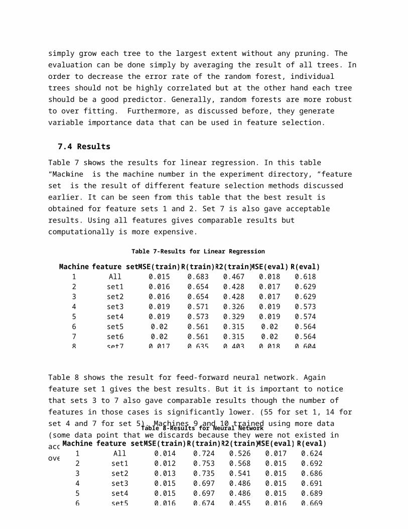
Table 7 shows the results for linear regression. In this table “Machine” is the machine number in the experiment directory, “feature set” is the result of different feature selection methods discussed earlier. It can be seen from this table that the best result is obtained for feature sets 1 and 2. Set 7 is also gave acceptable results. Using all features gives comparable results but computationally is more expensive.

Table 8 shows the result for feed-forward neural network. Again feature set 1 gives the best results. But it is important to notice that sets 3 to 7 also gave comparable results though the number of features in those cases is significantly lower. (55 for set 1, 14 for set 4 and 7 for set 5). Machines 9 and 10 trained using more data (some data point that we discards because they were not existed in acoustic dataset) As it is expected results gets better by training over a bigger data set.

Table 7-Results for Linear Regression

Machine feature set MSE(train) R(train) R2(train) MSE(eval) R(eval) R2(eval)1 All 0.015 0.683 0.467 0.018 0.618 0.3832 set1 0.016 0.654 0.428 0.017 0.629 0.3963 set2 0.016 0.654 0.428 0.017 0.629 0.3954 set3 0.019 0.571 0.326 0.019 0.573 0.3285 set4 0.019 0.573 0.329 0.019 0.574 0.3296 set5 0.02 0.561 0.315 0.02 0.564 0.3187 set6 0.02 0.561 0.315 0.02 0.564 0.3188 set7 0.017 0.635 0.403 0.018 0.604 0.365

Table 8-Results for Neural Network


9* All 0.017 0.742 0.551 0.016 0.67 0.45

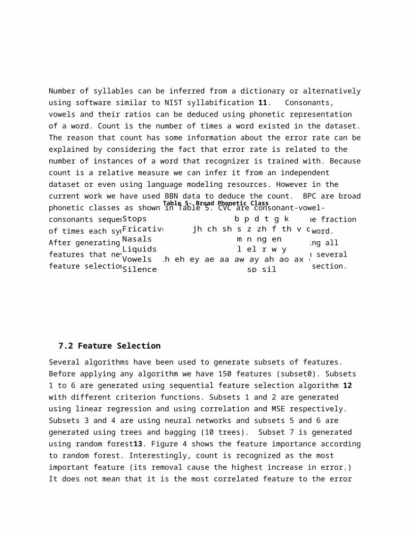
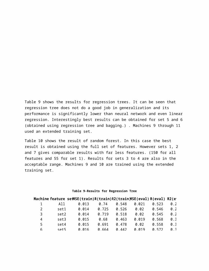
Table 9 shows the results for regression trees. It can be seen that regression tree does not do a good job in generalization and its performance is significantly lower than neural network and even linear regression. Interestingly best results can be obtained for set 5 and 6 (obtained using regression tree and bagging.) . Machines 9 through 11 used an extended training set.

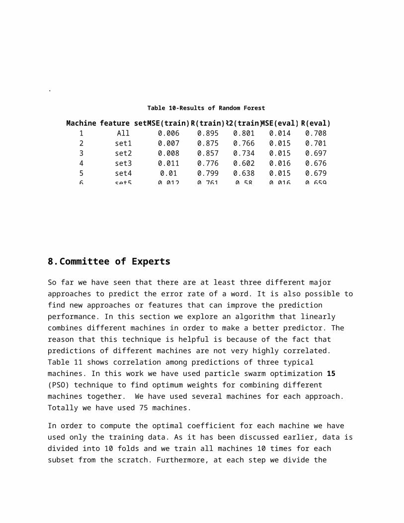
Table 10 shows the result of random forest. In this case the best result is obtained using the full set of features. However sets 1, 2 and 7 gives comparable results with far less features. (150 for all features and 55 for set 1). Results for sets 3 to 4 are also in the acceptable range. Machines 9 and 10 are trained using the extended training set.

.

Table 9-Results for Regression Tree


9* All 0.016 0.764 0.584 0.02 0.534 0.28510* set1 0.017 0.747 0.558 0.02 0.559 0.31311* set7 0.016 0.752 0.566 0.02 0.56 0.313

Table 10-Results of Random Forest


9* All 0.007 0.905 0.82 0.014 0.71 0.50410* set1 0.008 0.886 0.786 0.015 0.701 0.492

8. Committee of Experts

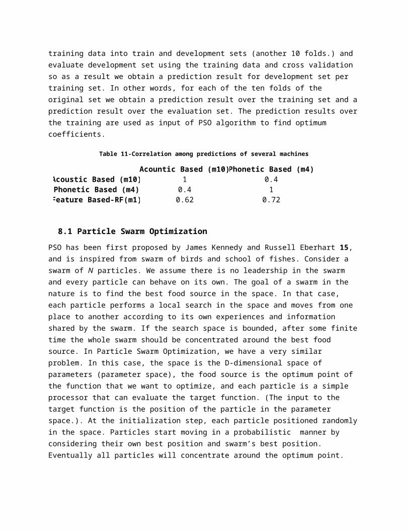
So far we have seen that there are at least three different major approaches to predict the error rate of a word. It is also possible to find new approaches or features that can improve the prediction performance. In this section we explore an algorithm that linearly combines different machines in order to make a better predictor. The reason that this technique is helpful is because of the fact that predictions of different machines are not very highly correlated. Table 11 shows correlation among predictions of three typical machines. In this work we have used particle swarm optimization 15 (PSO) technique to find optimum weights for combining different machines together. We have used several machines for each approach. Totally we have used 75 machines.

In order to compute the optimal coefficient for each machine we have used only the training data. As it has been discussed earlier, data is divided into 10 folds and we train all machines 10 times for each subset from the scratch. Furthermore, at each step we divide the training data into train and development sets (another 10 folds.) and evaluate development set using the training data and cross validation so as a result we obtain a prediction result for development set per training set. In other words, for each of the ten folds of the original set we obtain a prediction result over the training set and a prediction result over the evaluation set. The prediction results over the training are used as input of PSO algorithm to find optimum coefficients.

8.1 Particle Swarm Optimization

PSO has been first proposed by James Kennedy and Russell Eberhart 15, and is inspired from swarm of birds and school of fishes. Consider a swarm of N particles. We assume there is no leadership in the swarm and every particle can behave on its own. The goal of a swarm in the nature is to find the best food source in the space. In that case, each particle performs a local search in the space and moves from one place to another according to its own experiences and information shared by the swarm. If the search space is bounded, after some finite time the whole swarm should be concentrated around the best food source. In Particle Swarm Optimization, we have a very similar problem. In this case, the space is the D-dimensional space of parameters (parameter space), the food source is the optimum point of the function that we want to optimize, and each particle is a simple processor that can evaluate the target function. (The input to the target function is the position of the particle in the parameter space.). At the initialization step, each particle positioned randomly in the space. Particles start moving in a probabilistic manner by considering their own best position and swarm’s best position. Eventually all particles will concentrate around the optimum point.

In this work we have a linearly constrained problem in which we want to find optimum weights in such a way that they sum up to one. We have used CLPSO 16 for this constrained optimization problem.

Table 11-Correlation among predictions of several machines

Acountic Based (m10) Phonetic Based (m4) Feature Based-RF(m1)Acoustic Based (m10) 1 0.4 0.62Phonetic Based (m4) 0.4 1 0.72

Feature Based-RF(m1) 0.62 0.72 1

The goal of the algorithm is to minimize subject to . In this

problem and n is the number of coefficients and all elements of are equal to one. The algorithm is as follow:

1. Set iteration t to zero and initialize the particles randomly within the search space. Because the search space is a probability space we can use Dirichlet distribution with concentration parameter equal to one to initialize particles. This will insure that all constrained are hold. Equation 5

shows the definition of Dirichlet distribution. In this case all are equal together and all set to one and is the number of coefficients.

55\* MERGEFORMAT ()

2. Evaluate the performance of each particle.

3. Compare the best performance of each particle to its current performance and update the best performance.

4. Set the global best to the position of the particle with best performance.5. Change the velocity for each particle except for the global best particle according to equation 6.6. For the global best particle update the velocity according to equation 7.7. Move each particle according to equation 8.8. Let t:=t+19. Check for convergence, if the answer is no go to step 2 10. Report the position of the global best as the optimum solution.

66\* MERGEFORMAT ()

77\* MERGEFORMAT ()

88\* MERGEFORMAT ()

In these equations, is weight inertia, and are acceleration coefficients and should be between

zero and two. is the index of global best particle, is the scaling factor and with

the property that , or in other words lies in null space of . In or experiments we set

.

8.2 Results

Table 12 shows the result of our approach for combining all machines. The first row shows the result of all machines (75) in which 27 machines are acoustic based distance machines (different parameters or input types.), 8 machines are phonetic based and 40 machines are feature based. The last three columns show the percent of each type of machines contribution for the final prediction. As it can be seen from these numbers, feature based machines have more contribution due to their better performance and phonetic based machines have the least contribution. It is interesting to know that 43 (57.33%) machines have zero contribution. Rows two and three are corresponding to cases that we forced linear regression machine and linear regression and trees to have zero coefficients. As it can be seen the results are almost the same though excluding linear machines improve the results slightly. The best R-Square that can be obtained with this approach is 58.1 % which shows 16% improvement relative to the best result that can be obtained using individual machines. Figure 5 shows the predicted error rate versus reference error rate for all words and for the second row of Table 12. Particularly from this figure we can see the predictions are practically useful.

Table 12-Results of Optimal Combining of Machines

MSE(trian) R(train) R2(trian) MSE(eval) R(eval) R2(eval) Acoustic% Phonetic%

all 9.16E-04 0.913 0.834 0.012 0.76 0.578 41.13% 10.56% 48.32%

exclude linear8.40E-04 0.918 0.843 0.012 0.762 0.581 44.71% 15.79% 39.50%

9.11E-04 0.91 0.829 0.012 0.761 0.579 45.22% 18.22% 36.56%

Input Machines

Feature based%

exclude linear/tree

9. Discussion and Future Direction

In this project we have tried several ideas to predict the error rate of a given word using all of its available features. Some of these features can be obtained from the word (i.e. number of syllables or phonetic distance based approach) and some needs some kind of processing (i.e. count or acoustic based approach.). It has been shown that we can obtain useful perdition using current approaches. However, there are several other things that we can do to improve the final results. The first thing is to find new useful features. Intuitively features with some correlation with the error rate can be useful. One of the

features that can be tried is the confusability score of a word. This score can be defined using, for example, a phonetic distance measure as the sum of the distances of a word from all other words in the database (or more generally in the dictionary). Intuitively, a word with a smaller confusability score is expected to perform better. We can also define a confusability score based on acoustic distance. Another path is to use a boot strap like training. In this approach each machine is trained using a randomly sampled (with replacement) set from the data and for feature based machines we can also have a random number of features (selected randomly) for each machine. Because of successful results of this approach in other applications, we can expect some improvement of the final results.

10. Reference

x

[1] A. Harati and J. Picone, "Assessing Search Term Strength in Spoken Term Detection," in submitted

Figure 5-Error Rate prediction of the Final Super Machine

to the IEEE Statistical Signal Processing Workshop(SSP'12), Michigan, USA, August 2012.

[2] http://www.bbn.com/.

[3] J. G. Fiscus et al, "Results of the 2006 spoken term detection evaluation," in Procedinigs of Workshop Searching Spont. Conv. Speech, Amsterdam, NL, July 2007, pp. 45-50.

[4] D. Miller et al., "Rapid and Accurate Spoken Term Detection," in Proceedings of INTERSPEECH, Antwerp, Belgium, September 2007, pp. 314-317.

[5] nexidia. http://www.nexidia.com/technology/phonetic_search_technology.

[6] NIST. http://www.itl.nist.gov/iad/mig/tests/rt/2002/software.htm.

[7] E. C. Holliman, J. Mcdaniel J. J. Godfrey, "SWITCHBOARD: telephone speech corpus for research and development," in Proceding of IEEE International Conference on Acoustics, Speech, and Signal Processing (ICASSP) , San Francisco, California, USA, March 1992, pp. 517-520.

[8] K. Pelckmans, J.A.K. Suykens, and H.V. Hamme P. Karsmakers, "Fixed-Size Kernel Logistic Regression for Phoneme Classification," in Proceedings of INTERSPEECH, Antwerp Belgium, 2007, pp. 78-81.

[9] R. Wagner and M. Fischer, "The String-to-String correction problem," ACM, vol. 21, no. 1, pp. 168–173, January 1974.

[10] H.S. Elovitz et al., "Automatic Translation of English Text to Phonetics by Means of Letter-to-Sound Rules," Naval Research Laboratory, Washington, DC, NRL Report 7948, 1976.

[11] W. M. Fisher. (1997, June) tsyl: NIST Syllabification Software. [Online]. http://www.nist.gov/speech/tools

[12] Richard L. Bankert David W. Aha, "A comparative evaluation of sequential feature selection algorithms," in In Learning from Data: Artificial Intelligence and Statistics, Hans-Joachim Lenz Douglas H. Fisher, Ed., 1996, pp. 199-206.

[13] Leo Breiman, "Random Forests," Machine Learning, vol. 45, no. 1, pp. 5-32, October 2001.

[14] Christopher M. Bishop, Neural Networks for Pattern Recognition.: Oxford University Press, January 1996.

[15] J. Kennedy and R Eberhart, "Particle Swarm Optimization," in proceddings of IEEE International Conference on Neural Networks, Perth, WA , Australia, December 1995, pp. 1942–1948.

[16] U. Paquet and A. P. Engelbrecht, "A new particle swarm optimiser for linearly constrained optimisation," in Proceedings of the IEEE Congress on Evolutionary Computation, CEC 2003, vol. 1, Canberra-Australia, December 2003, pp. 227-233.

x

http://www.nist.gov/speech/tools

Documents

Introduction - isip.piconepress.com€¦ · Web viewThe problem that we are trying to solve is to predict the performance of a search term especially for spoken-term-detection (STD)