Embed Size (px)
Citation preview
Introduction
Prof. Sivarama Dandamudi
School of Computer Science
Carleton University
Carleton University © S. Dandamudi 2
Why Parallel Systems?
Increased execution speedMain motivation for many applications
Improved fault-tolerance and reliabilityMultiple resources provide improved FT and reliability
ExpandabilityProblem scaleupNew applications
Carleton University © S. Dandamudi 3
Three Metrics
SpeedupProblem size is fixed
Adding more processors should reduce time
Speedup on n processors S(n) is
Time on 1 processor system
Time on n-processor systemLinear speedup if S(n) = n for 0 1
Perfectly linear speedup if = 1
Carleton University © S. Dandamudi 4
Three Metrics (cont’d)
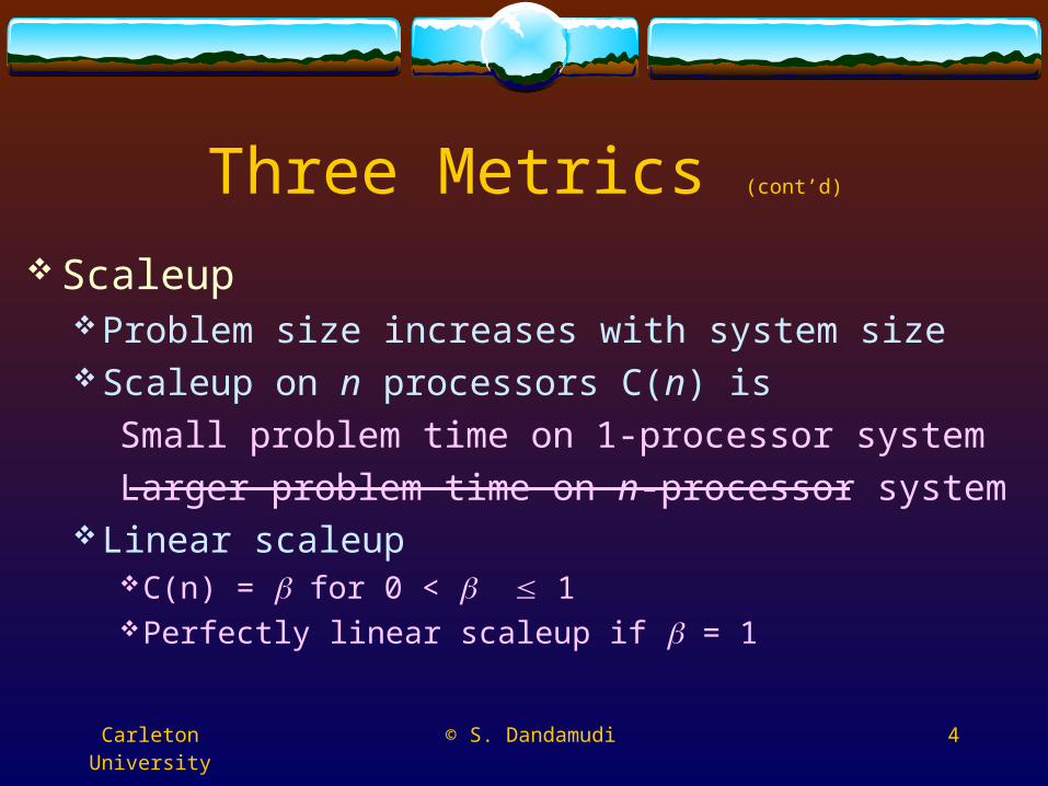
ScaleupProblem size increases with system sizeScaleup on n processors C(n) is
Small problem time on 1-processor system
Larger problem time on n-processor systemLinear scaleup
C(n) = for 0 < 1Perfectly linear scaleup if = 1
Carleton University © S. Dandamudi 5
Three Metrics (cont’d)
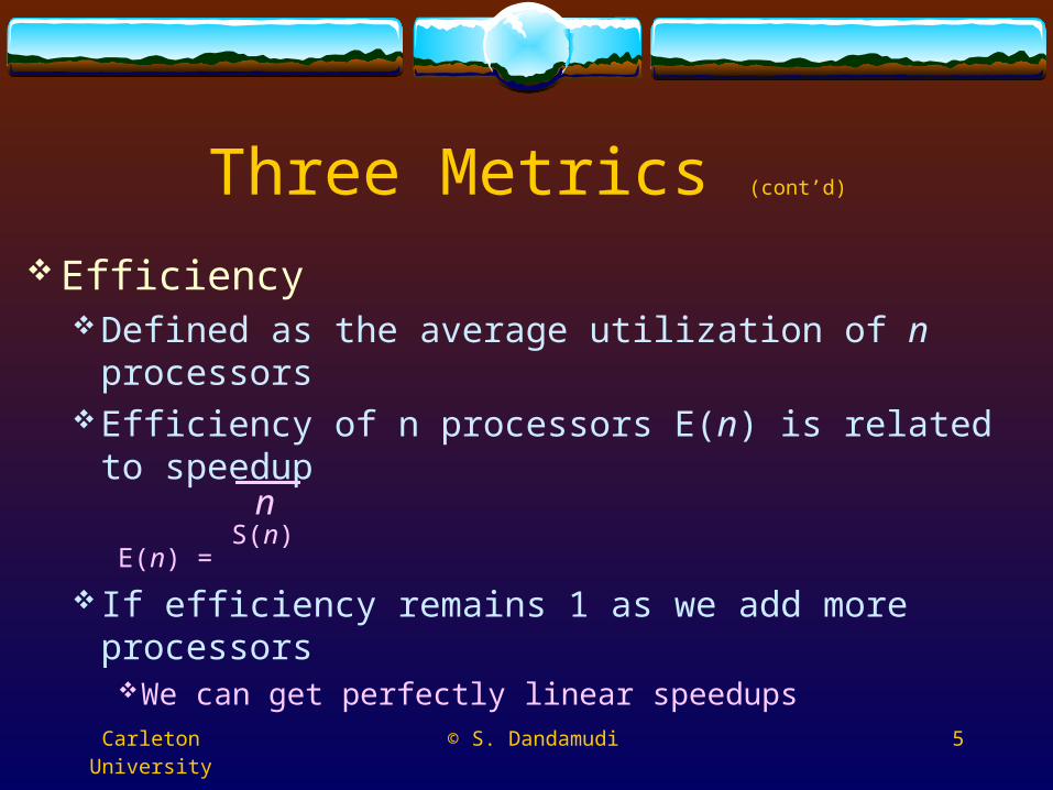
EfficiencyDefined as the average utilization of n processorsEfficiency of n processors E(n) is related to speedup
E(n) = S(n)
If efficiency remains 1 as we add more processorsWe can get perfectly linear speedups
n
Carleton University © S. Dandamudi 6
Three Metrics (cont’d)
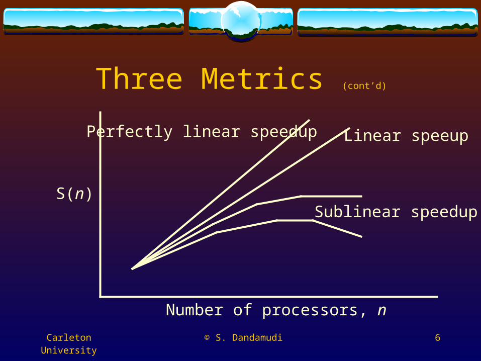
S(n)
Number of processors, n
Linear speeup
Sublinear speedup
Perfectly linear speedup
Carleton University © S. Dandamudi 7
Three Metrics (cont’d)
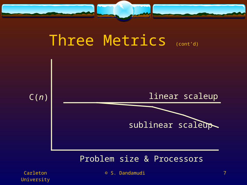
C(n)
Problem size & Processors
linear scaleup
sublinear scaleup
Carleton University © S. Dandamudi 8
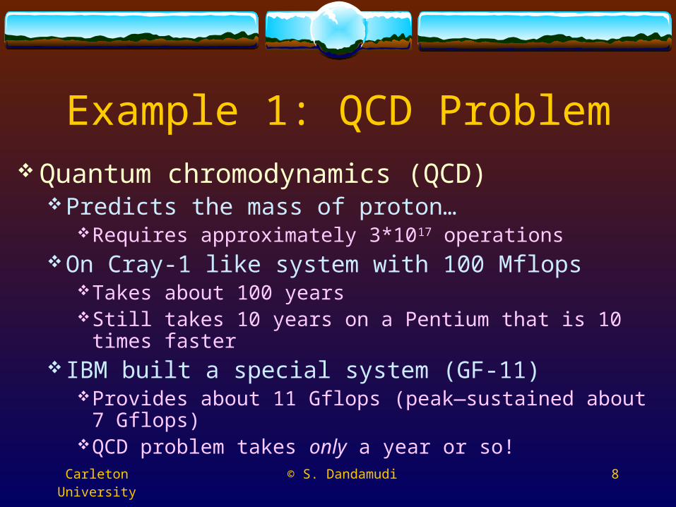
Example 1: QCD Problem Quantum chromodynamics (QCD)
Predicts the mass of proton…Requires approximately 3*1017 operations
On Cray-1 like system with 100 MflopsTakes about 100 yearsStill takes 10 years on a Pentium that is 10 times faster
IBM built a special system (GF-11)Provides about 11 Gflops (peak—sustained about 7 Gflops)QCD problem takes only a year or so!
Carleton University © S. Dandamudi 9
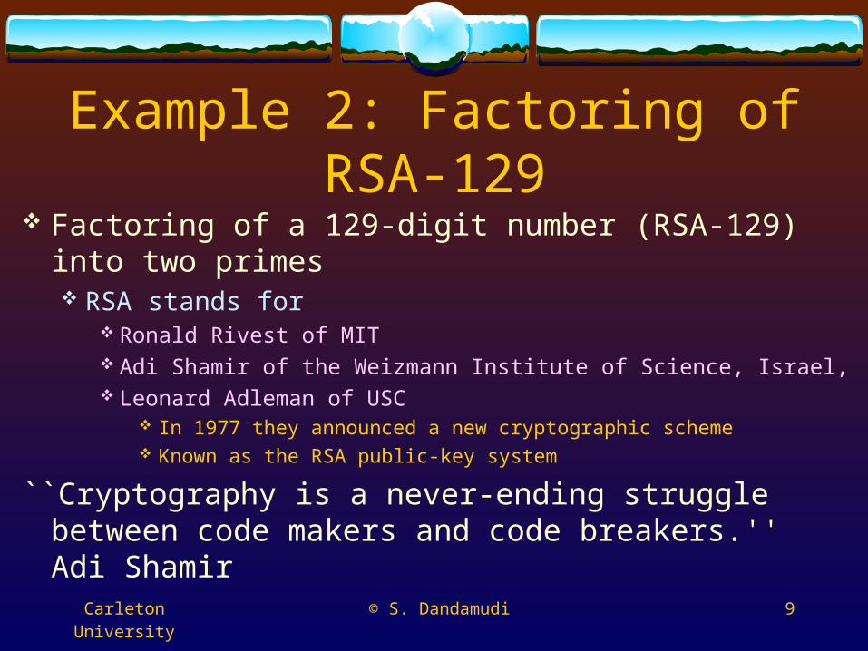
Example 2: Factoring of RSA-129 Factoring of a 129-digit number (RSA-129) into two
primes RSA stands for
Ronald Rivest of MIT Adi Shamir of the Weizmann Institute of Science, Israel, Leonard Adleman of USC
In 1977 they announced a new cryptographic scheme Known as the RSA public-key system
``Cryptography is a never-ending struggle between code makers and code breakers.'' Adi Shamir
Carleton University © S. Dandamudi 10
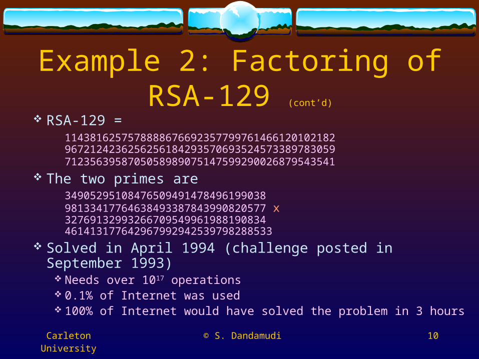
Example 2: Factoring of RSA-129 (cont’d)
RSA-129 = 1143816257578888676692357799761466120102182
9672124236256256184293570693524573389783059 7123563958705058989075147599290026879543541
The two primes are34905295108476509491478496199038 98133417764638493387843990820577 x32769132993266709549961988190834 461413177642967992942539798288533
Solved in April 1994 (challenge posted in September 1993) Needs over 1017 operations 0.1% of Internet was used 100% of Internet would have solved the problem in 3 hours
Carleton University © S. Dandamudi 11
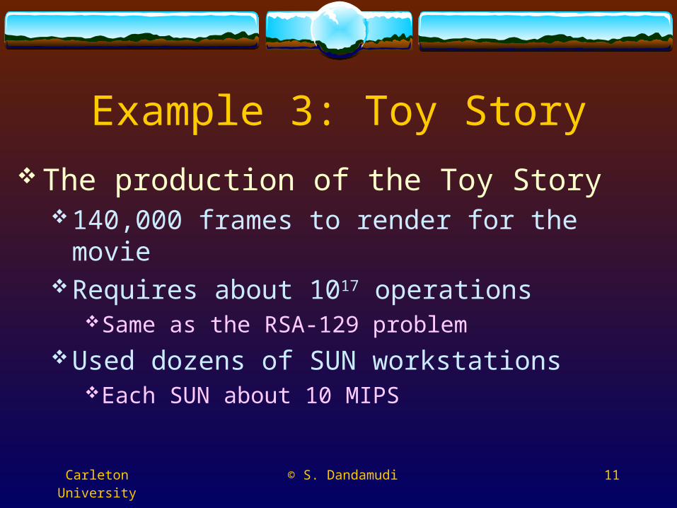
Example 3: Toy Story
The production of the Toy Story140,000 frames to render for the movieRequires about 1017 operations
Same as the RSA-129 problem
Used dozens of SUN workstationsEach SUN about 10 MIPS
Carleton University © S. Dandamudi 12
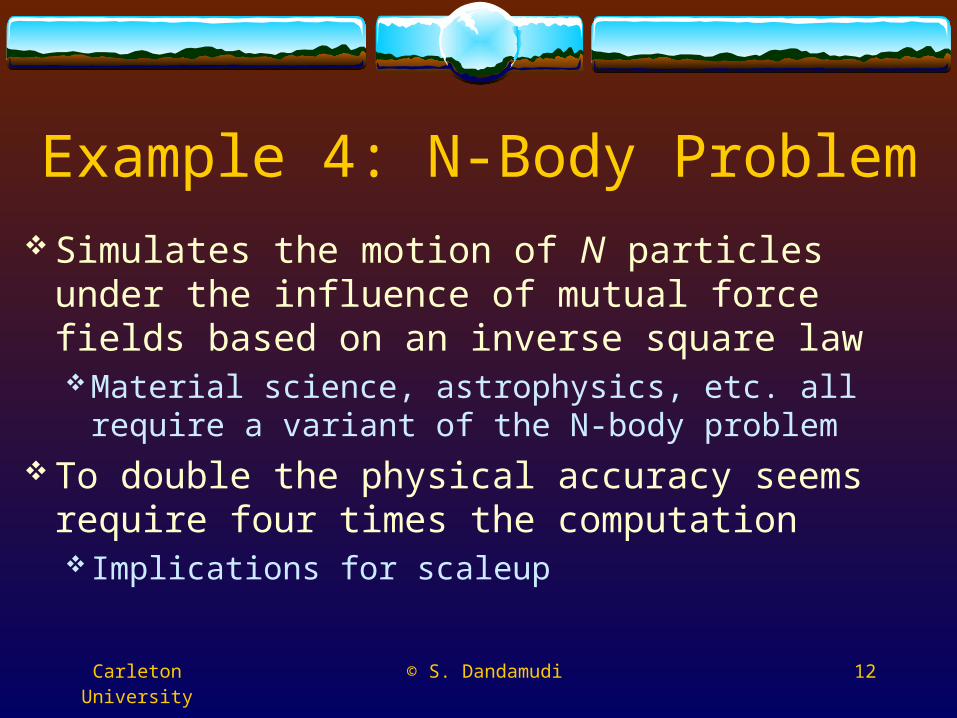
Example 4: N-Body Problem
Simulates the motion of N particles under the influence of mutual force fields based on an inverse square lawMaterial science, astrophysics, etc. all require a variant
of the N-body problem To double the physical accuracy seems require
four times the computation Implications for scaleup
Carleton University © S. Dandamudi 13
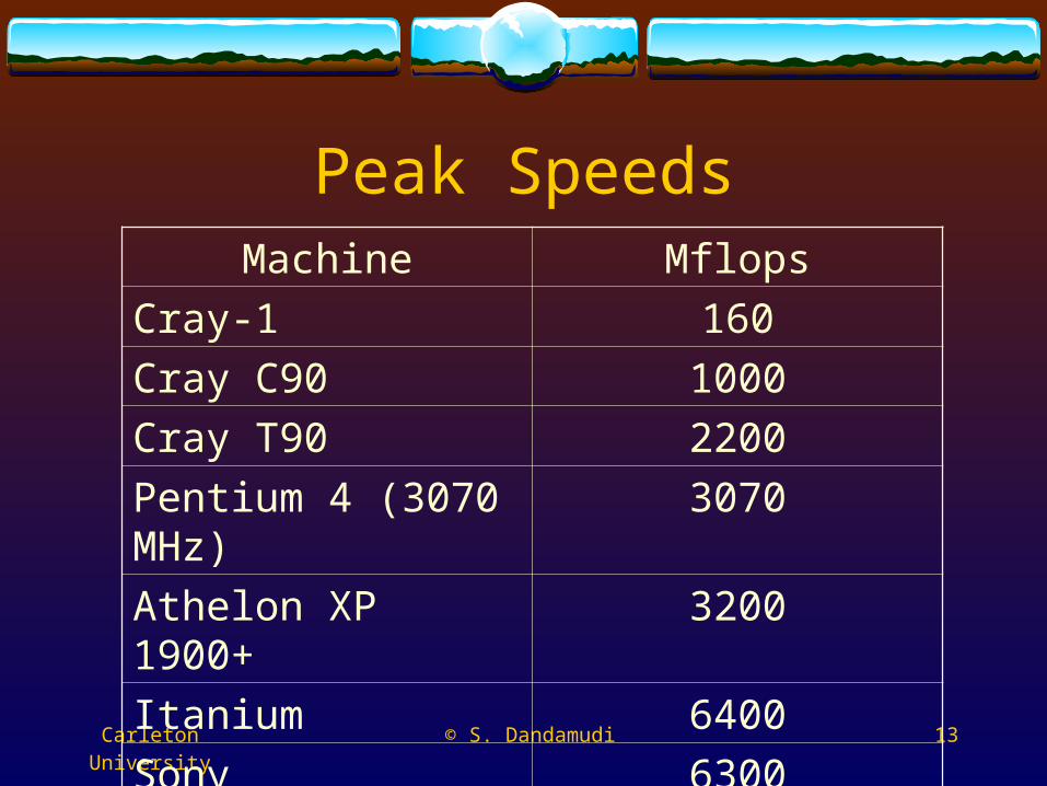
Peak SpeedsMachine Mflops
Cray-1 160
Cray C90 1000
Cray T90 2200
Pentium 4 (3070 MHz) 3070
Athelon XP 1900+ 3200
Itanium 6400
Sony Playstation 2 6300
Carleton University © S. Dandamudi 14
Applications of Parallel Systems A wide variety
Scientific applicationsEngineering applicationsDatabase applicationsArtificial intelligenceReal-time applicationsSpeech recognition Image processing
Carleton University © S. Dandamudi 15
Applications of Parallel Systems (cont’d)
Scientific applications Weather forecasting QCD Blood flow in the heart Molecular dynamics Evolution of galaxies
Most problems rely on basic operations of linear algebra Solving linear equations Finding Eigen values
Carleton University © S. Dandamudi 16
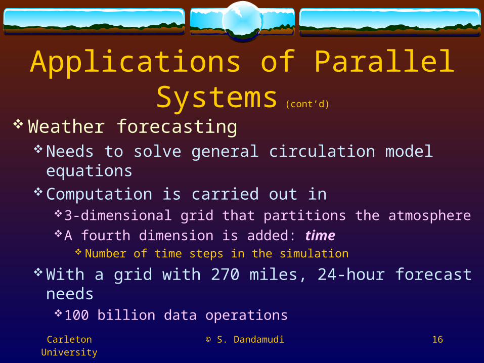
Applications of Parallel Systems (cont’d)
Weather forecastingNeeds to solve general circulation model equationsComputation is carried out in
3-dimensional grid that partitions the atmosphereA fourth dimension is added: time
Number of time steps in the simulation
With a grid with 270 miles, 24-hour forecast needs 100 billion data operations
Carleton University © S. Dandamudi 17
Applications of Parallel Systems (cont’d)
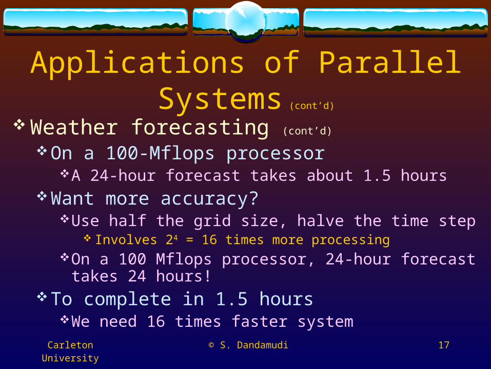
Weather forecasting (cont’d)
On a 100-Mflops processorA 24-hour forecast takes about 1.5 hours
Want more accuracy?Use half the grid size, halve the time step
Involves 24 = 16 times more processingOn a 100 Mflops processor, 24-hour forecast takes 24 hours!
To complete in 1.5 hoursWe need 16 times faster system
Carleton University © S. Dandamudi 18
Applications of Parallel Systems (cont’d)
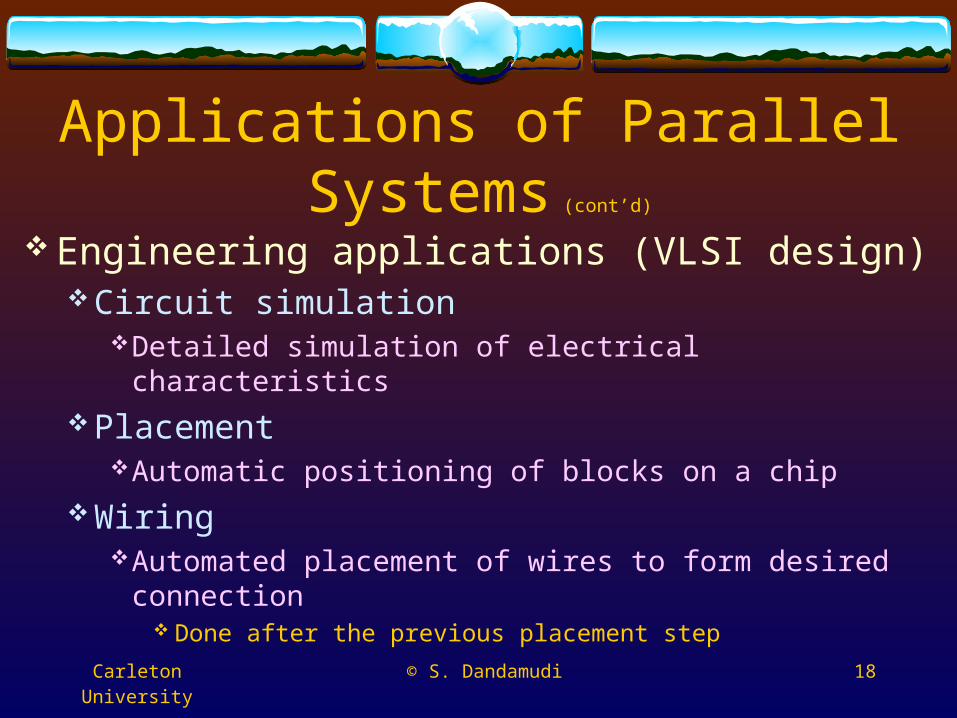
Engineering applications (VLSI design)Circuit simulation
Detailed simulation of electrical characteristics
PlacementAutomatic positioning of blocks on a chip
WiringAutomated placement of wires to form desired connection
Done after the previous placement step
Carleton University © S. Dandamudi 19
Applications of Parallel Systems (cont’d)
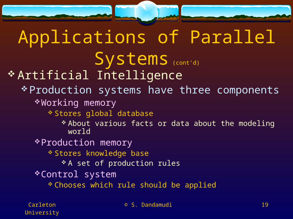
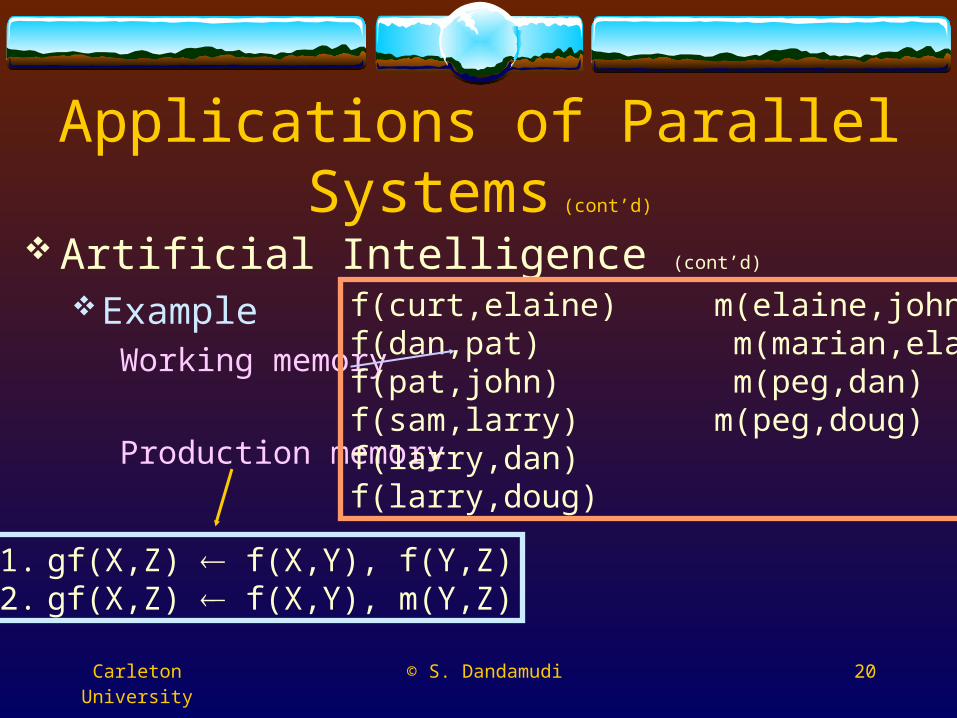
Artificial IntelligenceProduction systems have three components
Working memory Stores global database
About various facts or data about the modeling worldProduction memory
Stores knowledge base A set of production rules
Control system Chooses which rule should be applied
Carleton University © S. Dandamudi 20
Applications of Parallel Systems (cont’d)
Artificial Intelligence (cont’d)
ExampleWorking memory
Production memory
f(curt,elaine) m(elaine,john)f(dan,pat) m(marian,elaine)f(pat,john) m(peg,dan)f(sam,larry) m(peg,doug)f(larry,dan)f(larry,doug)
1. gf(X,Z) f(X,Y), f(Y,Z)2. gf(X,Z) f(X,Y), m(Y,Z)
Carleton University © S. Dandamudi 21
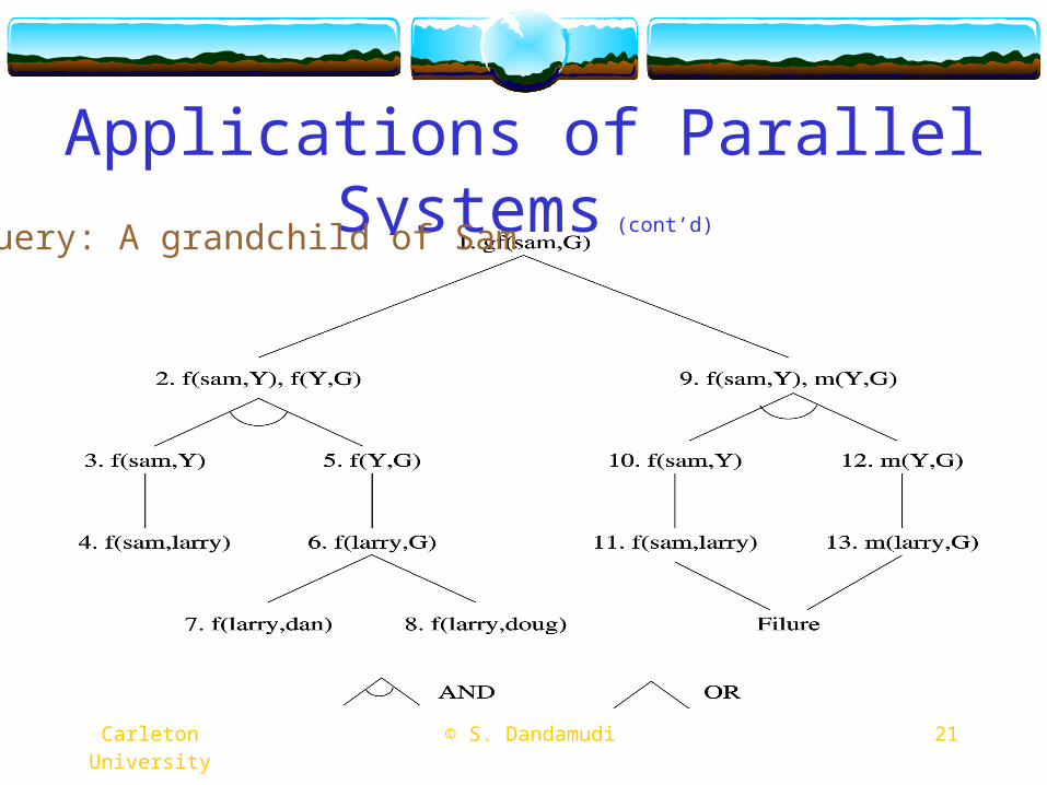
Applications of Parallel Systems (cont’d)
Query: A grandchild of Sam
Carleton University © S. Dandamudi 22
Applications of Parallel Systems (cont’d)
Artificial Intelligence (cont’d)
Sources of parallelismAssign each production rule its own processor
Each can search the working memory for pertinent facts in parallel with all the other processors
AND-parallelism Synchronization is involved
OR-parallelism Abort other searches if one is successful
Carleton University © S. Dandamudi 23
Applications of Parallel Systems (cont’d)
Database applicationsRelational model
Uses tables to store dataThree basic operations
Selection Selects tuples that satisfy a specified condition
Projection Selects certain specified columns
Join Combines data from two tables
Carleton University © S. Dandamudi 24
Applications of Parallel Systems (cont’d)
Database applications (cont’d)
Sources of parallelismWithin a single query (intra-query parallelism)
Horizontally partition relations into P fragments Each processor independently works on each segment
Among queries (inter-query parallelism) Execute several queries concurrently
Exploit common subqueries Improves query throughput
Carleton University © S. Dandamudi 25
Flynn’s Taxonomy
Based on number of instruction and data streamsSingle-Instruction, Single-Data stream (SISD)
Uniprocessor systems
Single-Instruction, Multiple-Data stream (SIMD)Array processors
Multiple-Instruction, Single-Data stream (MISD)Not really useful
Multiple-Instruction, Multiple-Data stream (MIMD)
Carleton University © S. Dandamudi 26
Flynn’s Taxonomy
MIMD systemsMost popular category
Shared-memory systemsAlso called multiprocessors
Sometimes called tightly-coupled systems
Distributed-memory systemsAlso called multicomputers
Sometimes called loosely-coupled systems
Carleton University © S. Dandamudi 27
Another Taxonomy Parallel systems
SynchronousVectorArraySIMDSystolic
AsynchronousMIMDDataflow
Carleton University © S. Dandamudi 28
SIMD Architecture Multiple actors, single script SIMD comes in two flavours
Array processors Large number of simple processors
Operate on small amount of data (bits, bytes, words,…) Illiac IV, Burroughs BSP, Connection Machine CM-1
Vector processors Small number (< 32) of powerful, pipelined processors
Operate on large amount of data (vectors) Cray 1 (1976), Cray X/MP (mid 1980s, 4 processors), Cray Y/MP (1988,
8 processors), Cray 3 (1989, 16 processors)
29 © S. Dandamudi Carleton University
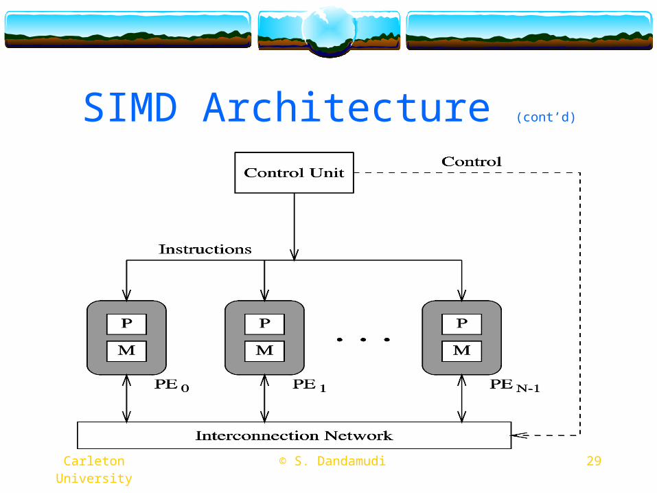
SIMD Architecture (cont’d)
Carleton University © S. Dandamudi 30
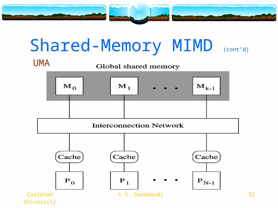
Shared-Memory MIMD Two major classes
UMAUniform memory accessTypically bus-basedLimited to small size systems
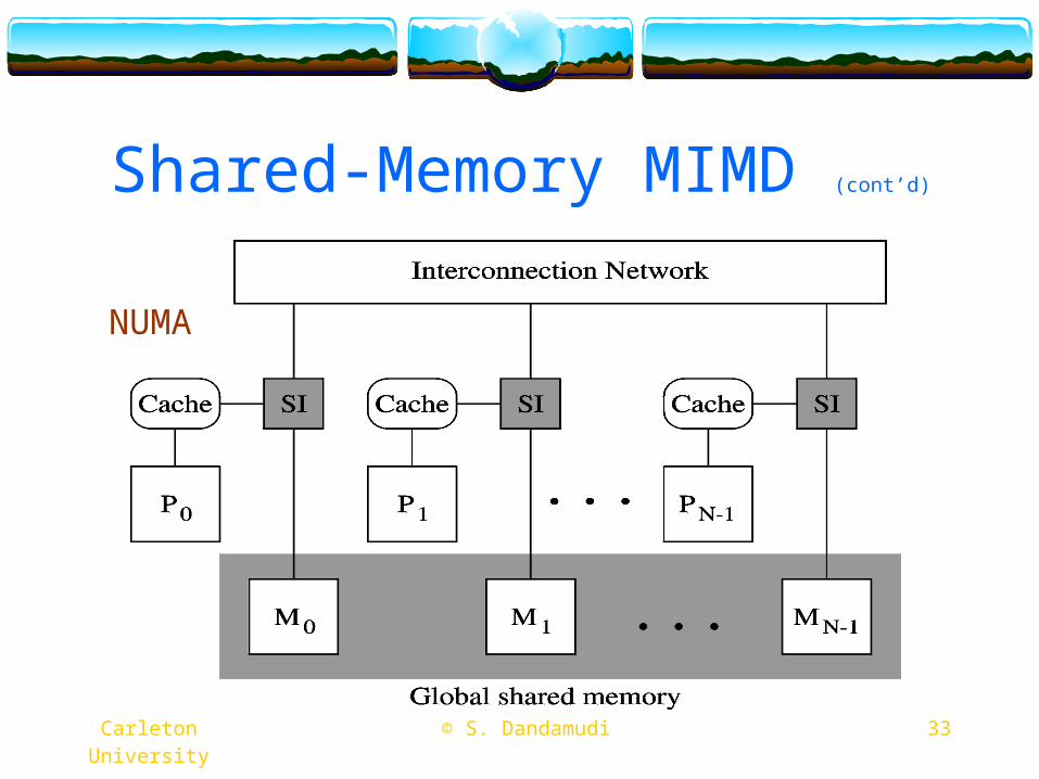
NUMANon-uniform memory accessUse a MIN-based interconnectionExpandable to medium system sizes
31 © S. Dandamudi Carleton University
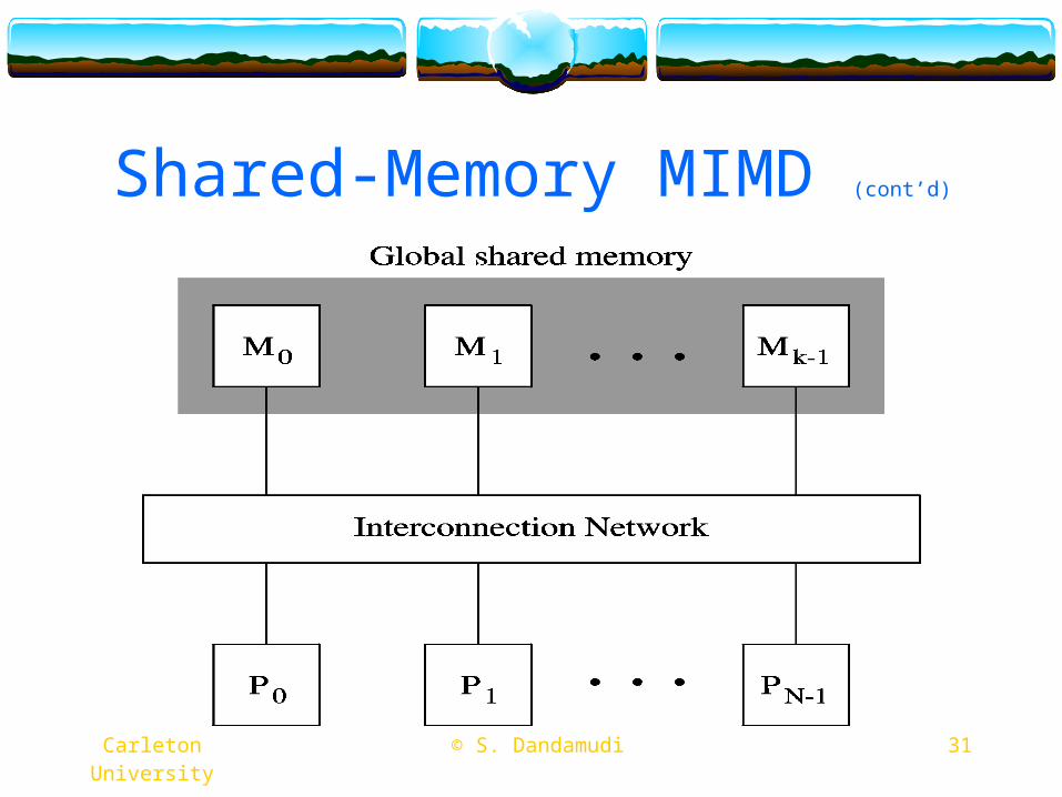
Shared-Memory MIMD (cont’d)
32 © S. Dandamudi Carleton University
Shared-Memory MIMD (cont’d)
UMA
33 © S. Dandamudi Carleton University
Shared-Memory MIMD (cont’d)
NUMA
Carleton University © S. Dandamudi 34
Shared-Memory MIMD (cont’d)
ExamplesSGI Power OnyxCray C90 IBM SP2 Node
Symmetric Multi-Processing (SMP)Special case of shared-memory MIMD Identical processors share the memory
Carleton University © S. Dandamudi 35
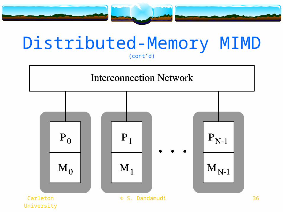
Distributed-Memory MIMD
Typically use message-passing Interconnection network is static
Point-to-point network
System scales up to thousands of nodes Intel TFLOPS system consists of 9000+ processors
Similar to cluster systemsPopular architecture for large parallel systems
36 © S. Dandamudi Carleton University
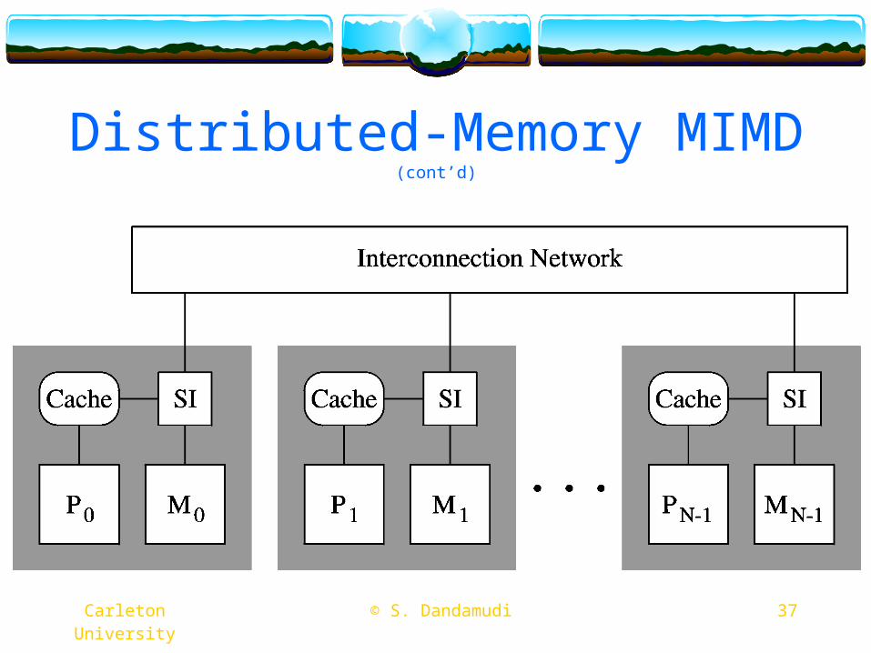
Distributed-Memory MIMD (cont’d)
37 © S. Dandamudi Carleton University
Distributed-Memory MIMD (cont’d)
38 © S. Dandamudi Carleton University
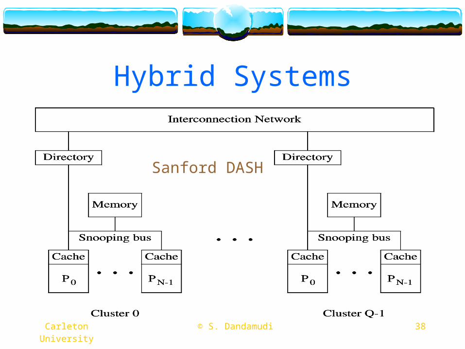
Hybrid Systems
Sanford DASH
Carleton University © S. Dandamudi 39
Distributed Shared Memory
Advantages of shared-memory MIMDRelatively easy to program
Global shared memory view
Fast communication & data sharingVia the shared memoryNo physical copying of data
Load distribution is not a problem
Carleton University © S. Dandamudi 40
Distributed Shared Memory (cont’d)
Disadvantages of shared-memory MIMDLimited scalability
UMA can scale to 10s of processorsNUMA can scale to 100s of processors
Expensive network
Carleton University © S. Dandamudi 41
Distributed Shared Memory (cont’d)
Advantages of distributed-memory MIMDGood scalability
Can scale to 1000s of processors
Inexpensive network (relatively speaking)Uses static interconnection
Cheaper to buildCan use off-the-shelf components
Carleton University © S. Dandamudi 42
Distributed Shared Memory (cont’d)
Disadvantages of distributed-memory MIMDNot easy to program
Deal with explicit message-passing
Slow networkExpensive data copying
Done by message passing
Load distribution is an issue
Carleton University © S. Dandamudi 43
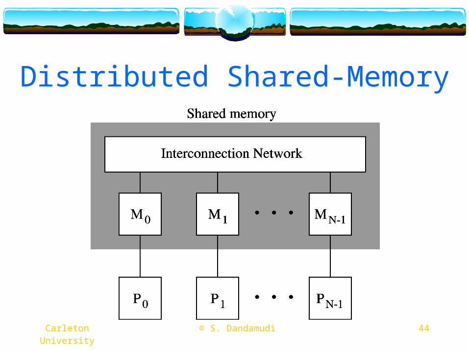
Distributed Shared Memory (cont’d)
DSM is proposed to take advantage of these two types of systemsUses distributed-memory MIMD hardwareA software layer gives the appearance of shared-
memory to the programmerA memory read, for example, is transparently converted to a
message send and reply
Example: Treadmarks from Rice
44 © S. Dandamudi Carleton University
Distributed Shared-Memory
Carleton University © S. Dandamudi 45
Cluster Systems Built with commodity processors
Cost-effectiveOften use the existing resources
Take advantage of the technological advances in commodity processors
Not tied to a single vendorGeneric components means
Competitive price Multiple sources of supply
Carleton University © S. Dandamudi 46
Cluster Systems (cont’d)
Several typesDedicated set of workstations (DoW)
Specifically built as a parallel systemRepresents one extremeDedicated to parallel workload
No serial workload
Closely related to the distributed-memory MIMD Communication network latency tends to be high
Example: Fast Ethernet
Carleton University © S. Dandamudi 47
Cluster Systems (cont’d)
Several types (cont’d)
Privately-owned workstations (PoW)Represents the other extremeAll workstations are privately owned
Idea is to harness unused processor cycles for parallel workload
Receives local jobs from owners Local jobs must receive higher priority
Workstations might be dynamically removed from the pool Owner shutting down/resetting the system, keyboard/mouse activity
Carleton University © S. Dandamudi 48
Cluster Systems (cont’d)
Several types (cont’d)
Community-owned workstations (CoW)All workstations are community-owned
Example: Workstations in a graduate labIn the middle of DoW and PoW
In PoW, a workstation could be removed when there is owner activity
Not so in CoW systems Parallel workload continues to run
Resource management should take these differences into account
Carleton University © S. Dandamudi 49
Cluster Systems (cont’d)
BeowulfUse PCs for parallel processingClosely resembles a DoW
Dedicated PCs (no scavenging of processor cycles)A private system network (not a shared one)Open design using public domain software and tools
Also known asPoPC (Pile of PCs)
Carleton University © S. Dandamudi 50
Cluster Systems (cont’d)
Beowulf (cont’d)
AdvantagesSystems not tied to a single manufacturer
Multiple vendors supply interchangeable components Leads to better pricing
Technology tracking is straightforwardIncremental expandability
Configure the system to match user needs Not limited to fixed, vendor-configured system
Carleton University © S. Dandamudi 51
Cluster Systems (cont’d)
Beowulf (cont’d)
Example systemLinux NetworX designed the largest and most powerful
Linux cluster Delivered to Lawrence Livermore National Lab (LLNL) in 2002 Uses 2,304 Intel 2.4 GHz Xeon processors
Peak rating: 11.2 Tflops Aggregate memory: 4.6 TB Aggregate disk space: 138.2 TB
Ranked 5th fastest supercomputer in the world
52 © S. Dandamudi Carleton University
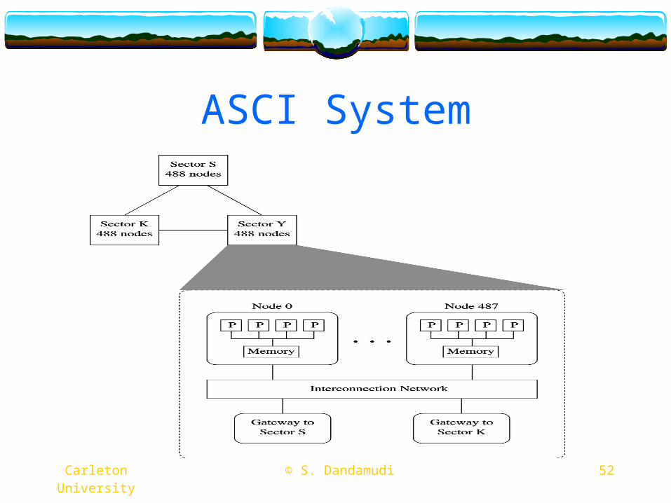
ASCI System
Carleton University © S. Dandamudi 53
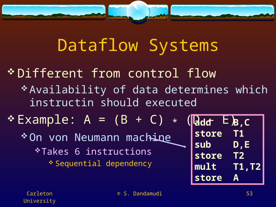
Dataflow Systems
Different from control flowAvailability of data determines which instructin should
executed
Example: A = (B + C) * (D – E)On von Neumann machine
Takes 6 instructions Sequential dependency
add B,Cstore T1sub D,Estore T2mult T1,T2store A
Carleton University © S. Dandamudi 54
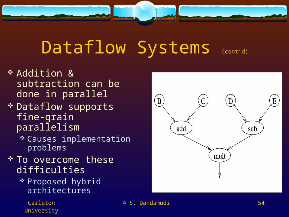
Dataflow Systems (cont’d)
Addition & subtraction can be done in parallel
Dataflow supports fine-grain parallelism Causes implementation
problems To overcome these
difficulties Proposed hybrid
architectures
Carleton University © S. Dandamudi 55
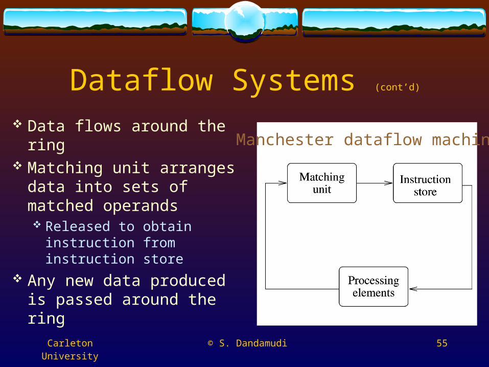
Dataflow Systems (cont’d)
Data flows around the ring Matching unit arranges
data into sets of matched operands Released to obtain
instruction from instruction store
Any new data produced is passed around the ring
Manchester dataflow machine
Carleton University © S. Dandamudi 56
Interconnection Networks
A critical component in many parallel systems Four design issues
Mode of operationControl strategySwitching methodTopology
Carleton University © S. Dandamudi 57
Interconnection Networks (cont’d)
Mode of operationRefers to the type of communication usedAsynchronous
Typically used in MIMD
SynchronousTypically used in SIMD
Mixed
Carleton University © S. Dandamudi 58
Interconnection Networks (cont’d)
Control strategyRefers to how routing is achieved
Centralized control Can cause scalability problem Reliability is an issue Non-uniform node structure
Distributed control Uniform node structure Improved reliability Improved scalability
Carleton University © S. Dandamudi 59
Interconnection Networks (cont’d)
Switching methodTwo basic types
Circuit switching A complete path is established Good for large data transmission Causes problems at high loads
Packet switching Uses store-and-forward method Good for short messages High latency
Carleton University © S. Dandamudi 60
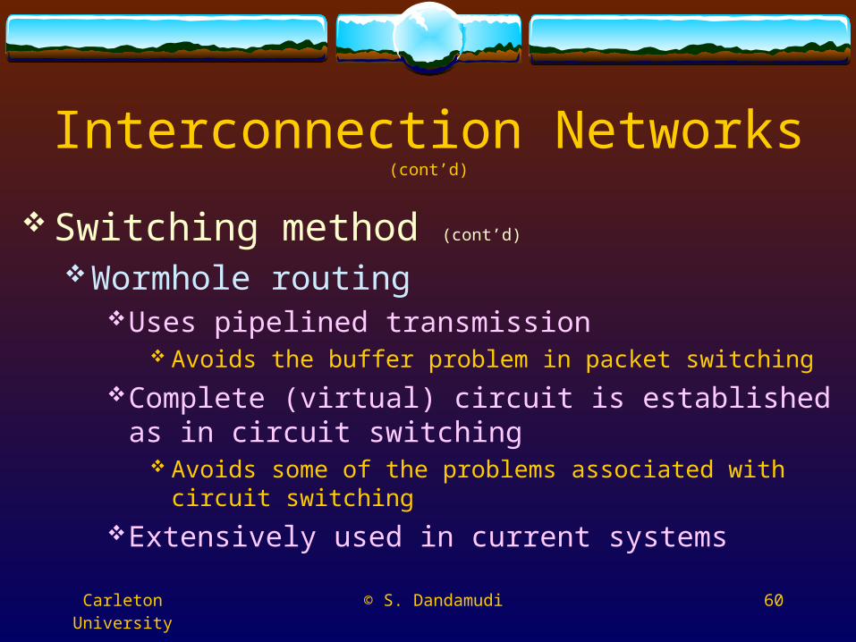
Interconnection Networks (cont’d)
Switching method (cont’d)
Wormhole routingUses pipelined transmission
Avoids the buffer problem in packet switching
Complete (virtual) circuit is established as in circuit switching
Avoids some of the problems associated with circuit switching
Extensively used in current systems
Carleton University © S. Dandamudi 61
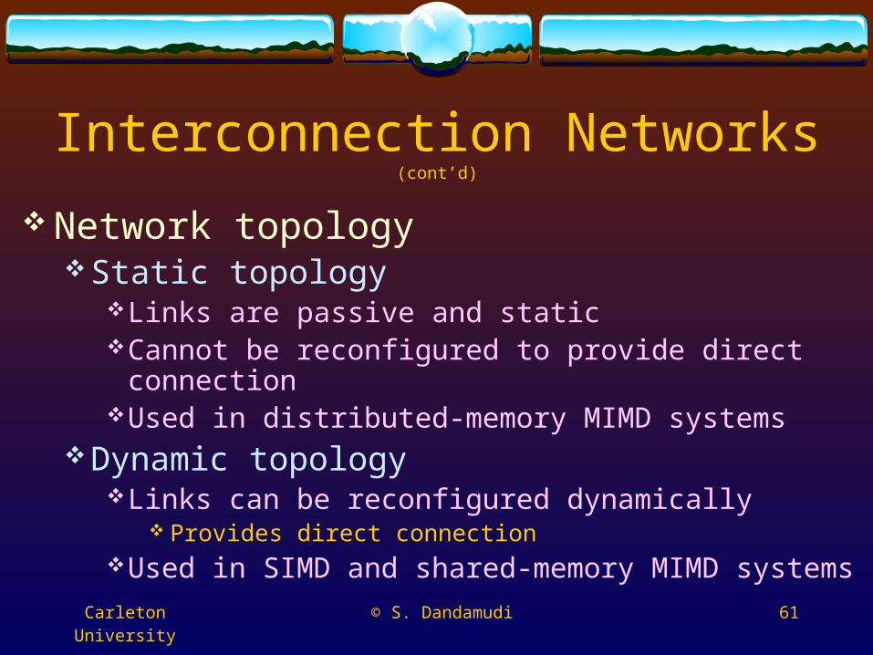
Interconnection Networks (cont’d)
Network topologyStatic topology
Links are passive and staticCannot be reconfigured to provide direct connectionUsed in distributed-memory MIMD systems
Dynamic topologyLinks can be reconfigured dynamically
Provides direct connectionUsed in SIMD and shared-memory MIMD systems
Carleton University © S. Dandamudi 62
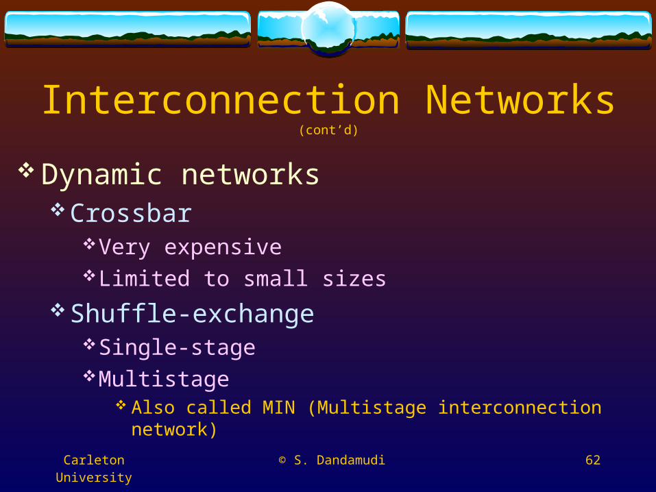
Interconnection Networks (cont’d)
Dynamic networksCrossbar
Very expensiveLimited to small sizes
Shuffle-exchangeSingle-stageMultistage
Also called MIN (Multistage interconnection network)
63 © S. Dandamudi Carleton University
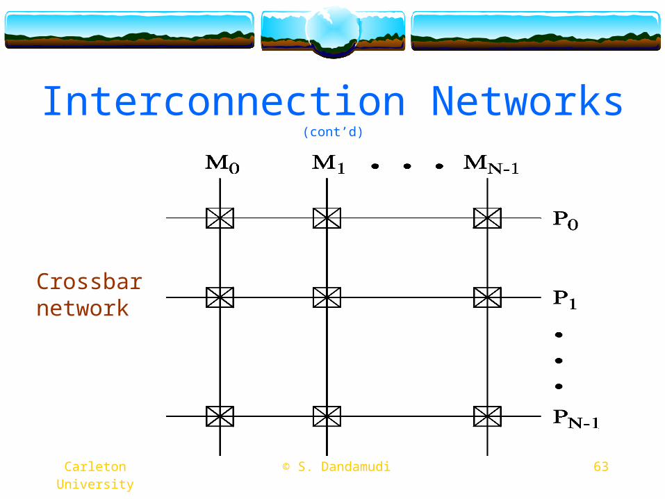
Interconnection Networks (cont’d)
Crossbarnetwork
Carleton University © S. Dandamudi 64
Interconnection Networks (cont’d)
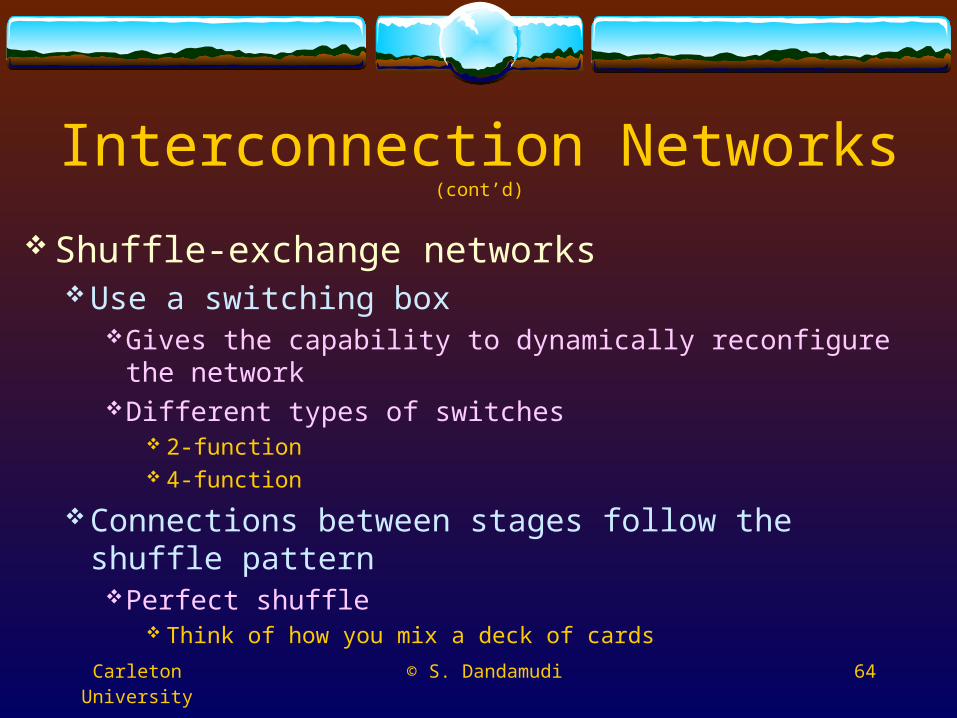
Shuffle-exchange networksUse a switching box
Gives the capability to dynamically reconfigure the networkDifferent types of switches
2-function 4-function
Connections between stages follow the shuffle patternPerfect shuffle
Think of how you mix a deck of cards
65 © S. Dandamudi Carleton University
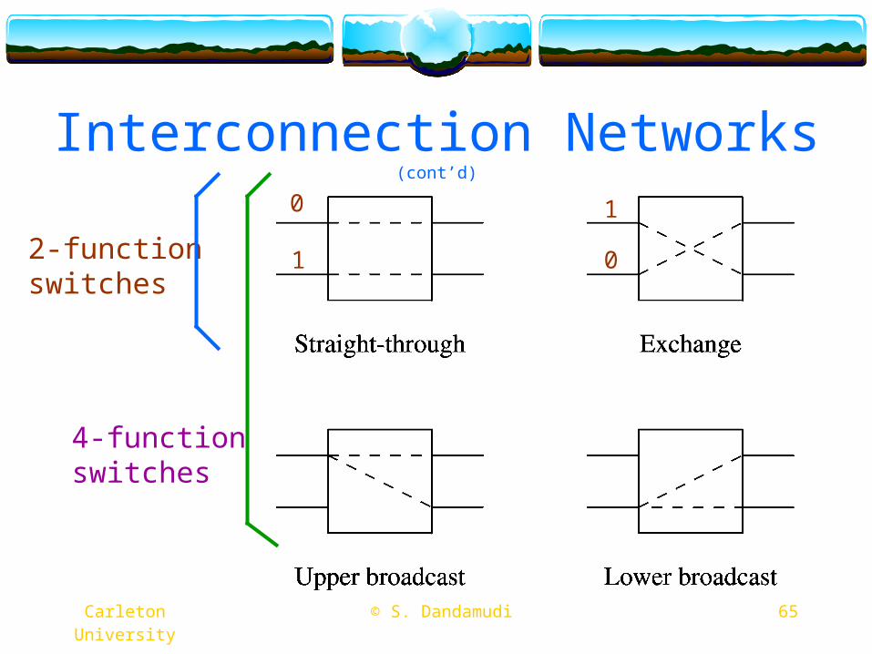
Interconnection Networks (cont’d)
2-function switches
4-function switches
0
1 0
1
66 © S. Dandamudi Carleton University
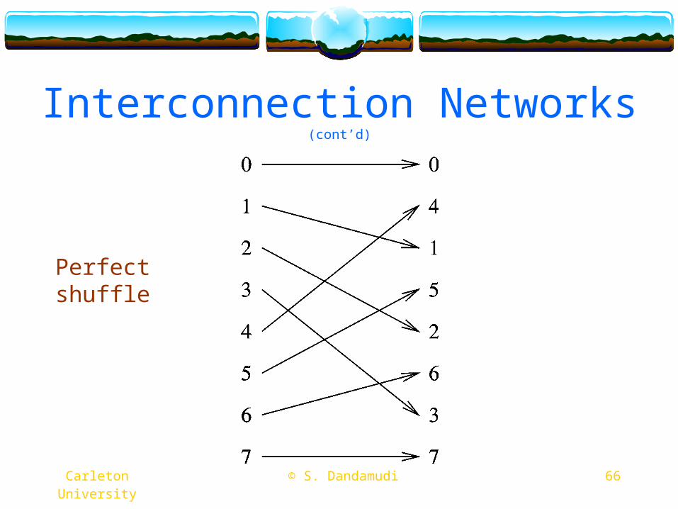
Interconnection Networks (cont’d)
Perfect shuffle
67 © S. Dandamudi Carleton University
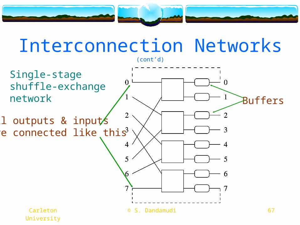
Interconnection Networks (cont’d)
Buffers
All outputs & inputs are connected like this
Single-stage shuffle-exchange network
68 © S. Dandamudi Carleton University
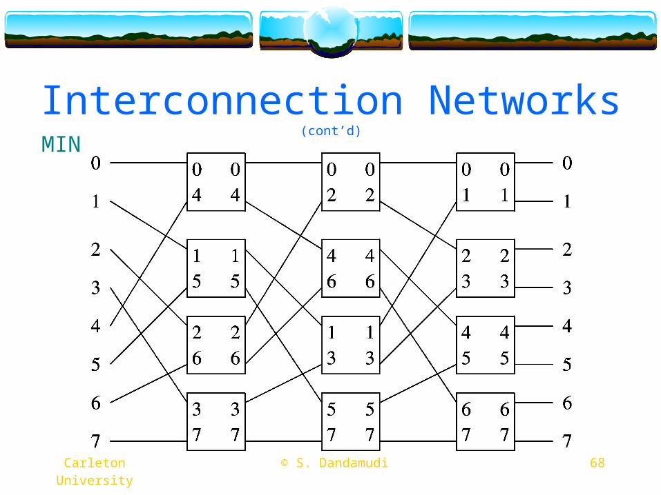
Interconnection Networks (cont’d)
MIN
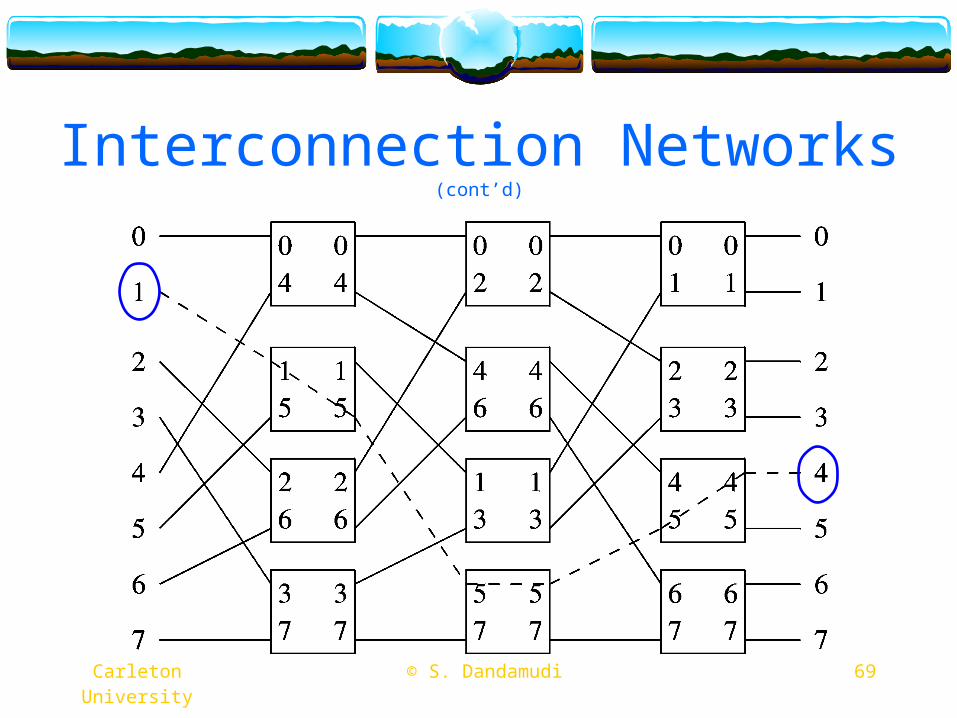
69 © S. Dandamudi Carleton University
Interconnection Networks (cont’d)
70 © S. Dandamudi Carleton University
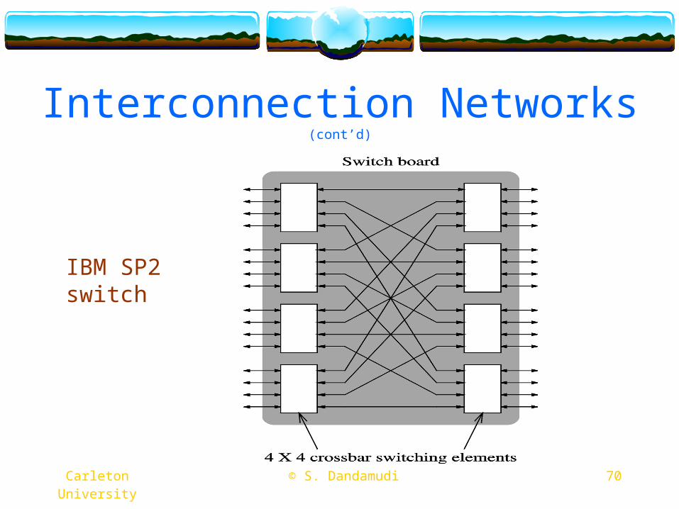
Interconnection Networks (cont’d)
IBM SP2 switch
Carleton University © S. Dandamudi 71
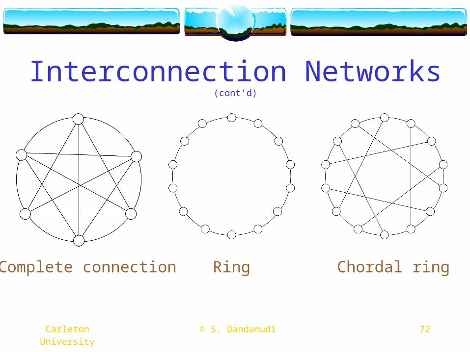
Interconnection Networks (cont’d)
Static interconnection networksComplete connection
One extremeHigh cost, low latency
Ring networkOther extremeLow cost, high latency
A variety of networks between these two extremes
Carleton University © S. Dandamudi 72
Interconnection Networks (cont’d)
Complete connection Ring Chordal ring
Carleton University © S. Dandamudi 73
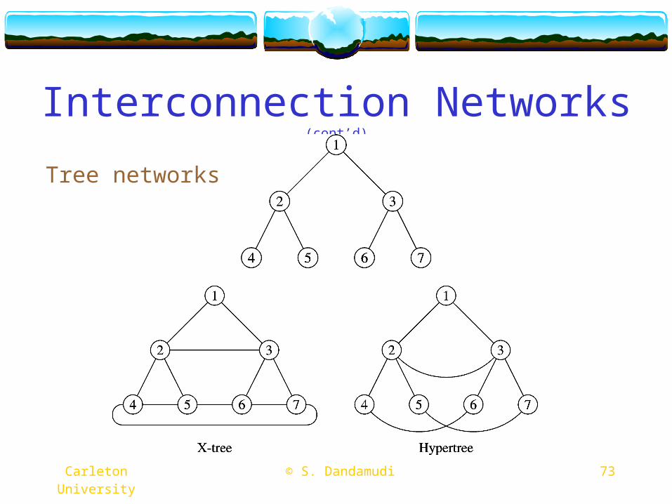
Interconnection Networks (cont’d)
Tree networks
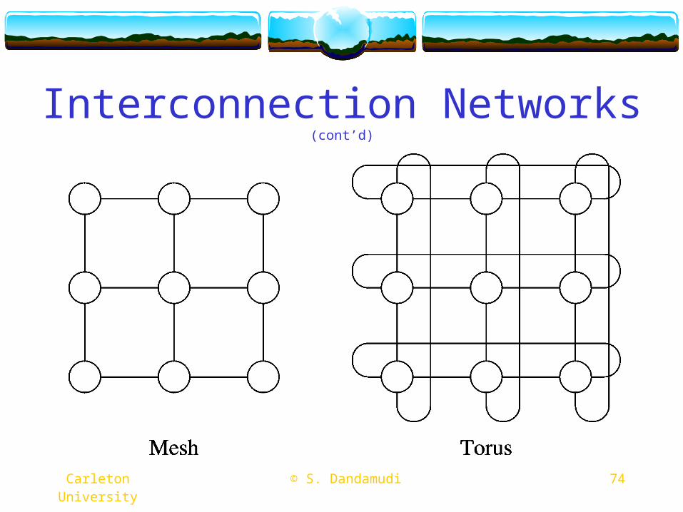
Carleton University © S. Dandamudi 74
Interconnection Networks (cont’d)
Carleton University © S. Dandamudi 75
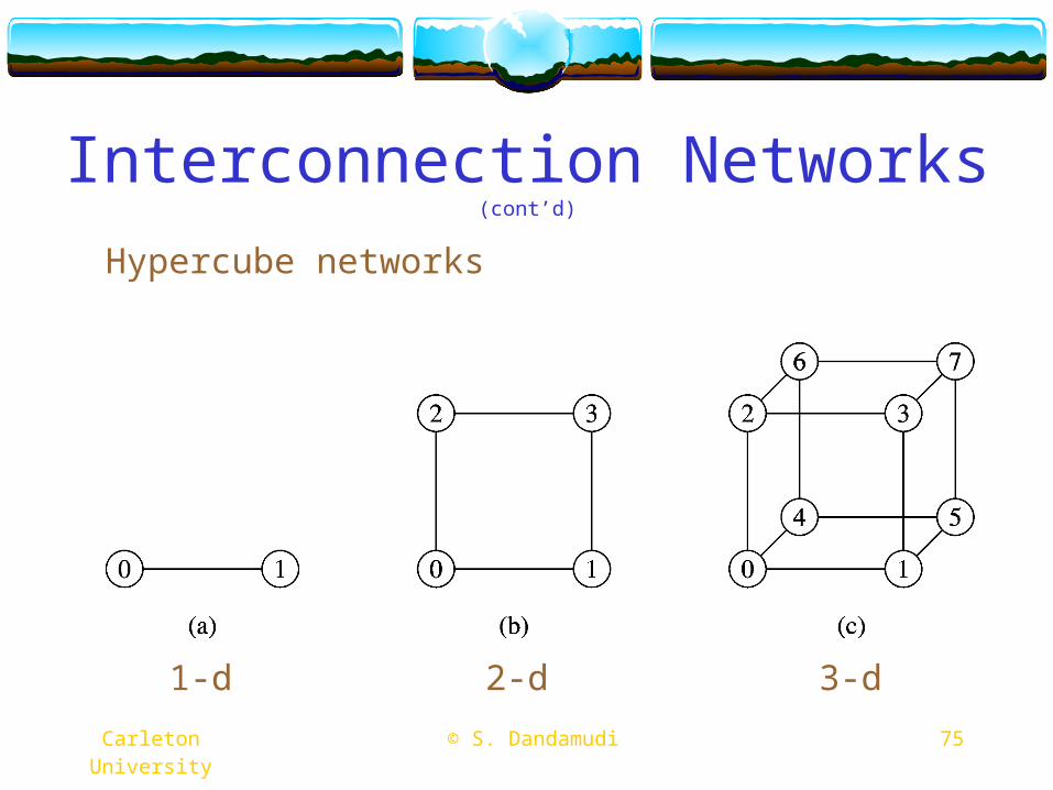
Interconnection Networks (cont’d)
Hypercube networks
1-d 2-d 3-d
Carleton University © S. Dandamudi 76
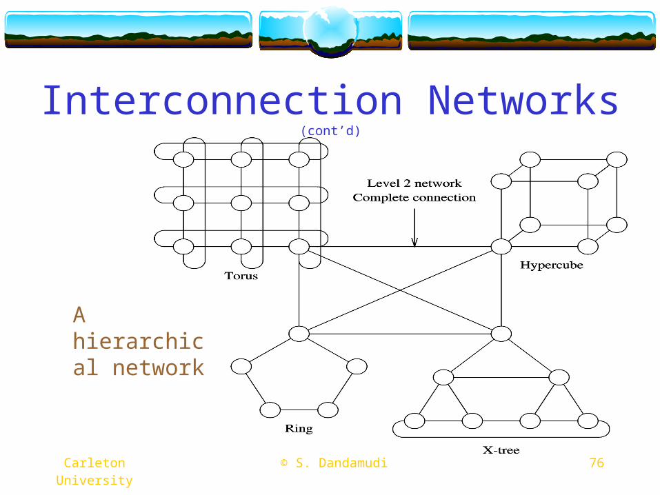
Interconnection Networks (cont’d)
A hierarchical network
Carleton University © S. Dandamudi 77
Future Parallel Systems
Special-purpose systems+ Very efficient
+ Relatively simple
- Narrow domain of applications
May be cost-effectiveDepends on the application
Carleton University © S. Dandamudi 78
Future Parallel Systems (cont’d)
General-purpose systems+ Cost-effective
+ Wide range of applications
Decreased speed
Decreased hardware utilization
Increased software requirements
Carleton University © S. Dandamudi 79
Future Parallel Systems (cont’d)
In favour of special-purpose systemsHarold Stone argues
Major advantage of general-purpose systems is that they are
economical due to their wide area of applicability
Economics of computer systems is changing rapidly because
of VLSI
Makes the special-purpose systems economically viable

Carleton University © S. Dandamudi 80
Future Parallel Systems (cont’d)
In favour of both types of systemsGajski argues
Problem space is constantly expandingSpecial-purpose systems can only be designed to solve
“mature” problemsAlways new applications for which no “standardized”
solution existsFor these applications, general-purpose systems are useful
Carleton University © S. Dandamudi 81
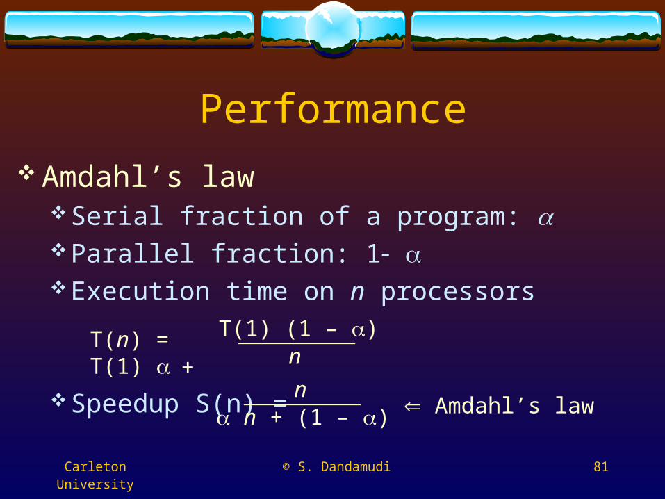
Performance
Amdahl’s lawSerial fraction of a program: Parallel fraction: 1 Execution time on n processors
Speedup S(n) =
T(n) = T(1)
T(1) (1 – )n
n n + (1 – ) Amdahl’s law
Carleton University © S. Dandamudi 82
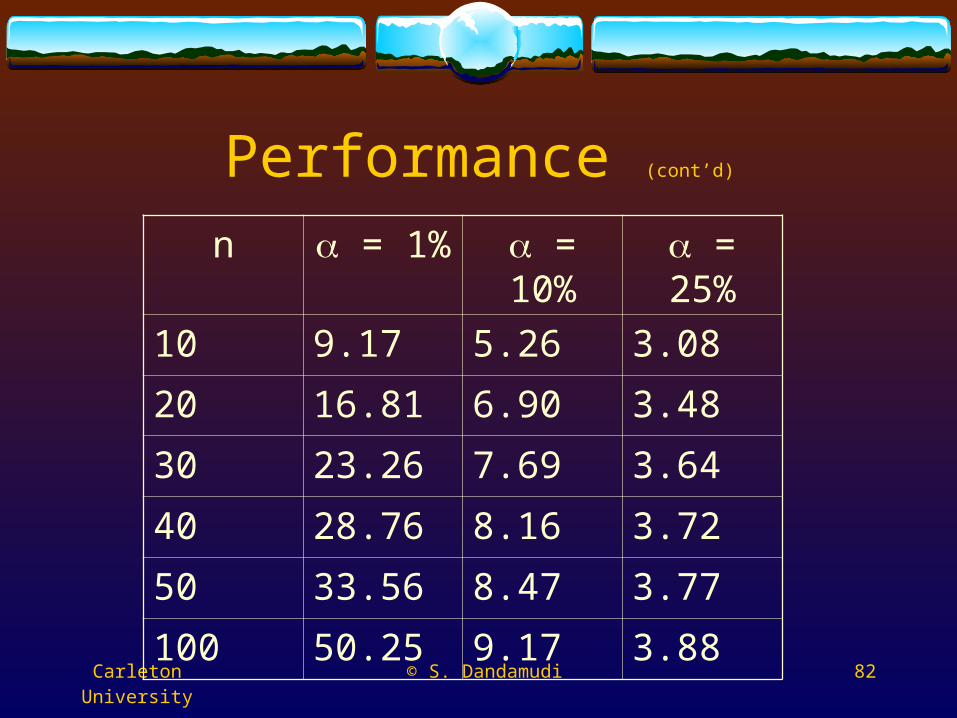
Performance (cont’d)
n = 1% = 10% = 25%
10 9.17 5.26 3.08
20 16.81 6.90 3.48
30 23.26 7.69 3.64
40 28.76 8.16 3.72
50 33.56 8.47 3.77
100 50.25 9.17 3.88
Carleton University © S. Dandamudi 83
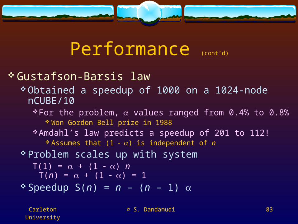
Performance (cont’d)
Gustafson-Barsis lawObtained a speedup of 1000 on a 1024-node nCUBE/10
For the problem, values ranged from 0.4% to 0.8% Won Gordon Bell prize in 1988
Amdahl’s law predicts a speedup of 201 to 112! Assumes that (1 ) is independent of n
Problem scales up with systemT(1) = + (1 ) n T(n) = + (1 ) = 1
Speedup S(n) = n – (n – 1)
Carleton University © S. Dandamudi 84
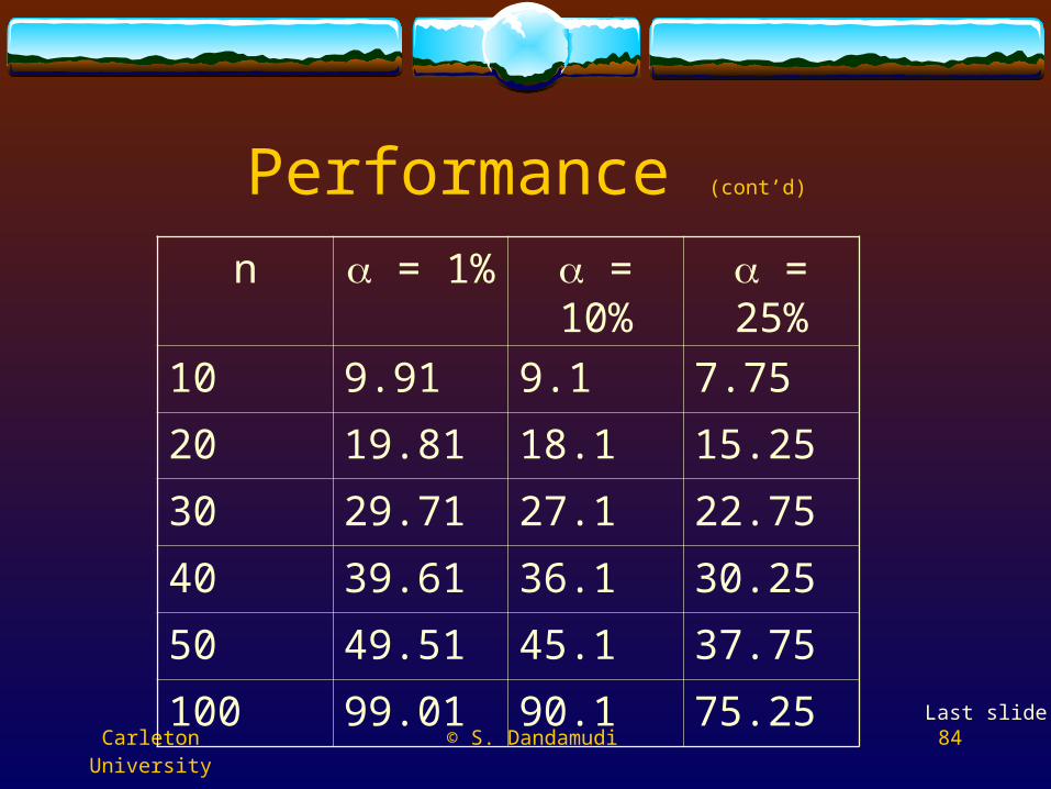
Performance (cont’d)
n = 1% = 10% = 25%
10 9.91 9.1 7.75
20 19.81 18.1 15.25
30 29.71 27.1 22.75
40 39.61 36.1 30.25
50 49.51 45.1 37.75
100 99.01 90.1 75.25Last slide