INTRODUCTION TO MATLAB FORENGINEERING STUDENTS

David HoucqueNorthwestern University

Contents

1 Tutorial lessons 1 1

1.1 Introduction . . . . . . . . . . . . . . . . . . . . . . . . . . . . . . . . . . . . 1

1.2 Basic features . . . . . . . . . . . . . . . . . . . . . . . . . . . . . . . . . . . 2

1.3 A minimum MATLAB session . . . . . . . . . . . . . . . . . . . . . . . . . . 2

1.3.1 Starting MATLAB . . . . . . . . . . . . . . . . . . . . . . . . . . . . 2

1.3.2 Using MATLAB as a calculator . . . . . . . . . . . . . . . . . . . . . 4

1.3.3 Quitting MATLAB . . . . . . . . . . . . . . . . . . . . . . . . . . . . 5

1.4 Getting started . . . . . . . . . . . . . . . . . . . . . . . . . . . . . . . . . . 5

1.4.1 Creating MATLAB variables . . . . . . . . . . . . . . . . . . . . . . . 5

1.4.2 Overwriting variable . . . . . . . . . . . . . . . . . . . . . . . . . . . 6

1.4.3 Error messages . . . . . . . . . . . . . . . . . . . . . . . . . . . . . . 6

1.4.4 Making corrections . . . . . . . . . . . . . . . . . . . . . . . . . . . . 6

1.4.5 Controlling the hierarchy of operations or precedence . . . . . . . . . 6

1.4.6 Controlling the appearance of floating point number . . . . . . . . . . 8

1.4.7 Managing the workspace . . . . . . . . . . . . . . . . . . . . . . . . . 9

1.4.8 Keeping track of your work session . . . . . . . . . . . . . . . . . . . 9

1.4.9 Entering multiple statements per line . . . . . . . . . . . . . . . . . . 10

1.4.10 Miscellaneous commands . . . . . . . . . . . . . . . . . . . . . . . . . 10

1.4.11 Getting help . . . . . . . . . . . . . . . . . . . . . . . . . . . . . . . . 10

1.5 Exercises . . . . . . . . . . . . . . . . . . . . . . . . . . . . . . . . . . . . . . 11

2 Tutorial lessons 2 12

2.1 Mathematical functions . . . . . . . . . . . . . . . . . . . . . . . . . . . . . . 12

2.1.1 Examples . . . . . . . . . . . . . . . . . . . . . . . . . . . . . . . . . 13

i

2.2 Basic plotting . . . . . . . . . . . . . . . . . . . . . . . . . . . . . . . . . . . 14

2.2.1 overview . . . . . . . . . . . . . . . . . . . . . . . . . . . . . . . . . . 14

2.2.2 Creating simple plots . . . . . . . . . . . . . . . . . . . . . . . . . . . 14

2.2.3 Adding titles, axis labels, and annotations . . . . . . . . . . . . . . . 15

2.2.4 Multiple data sets in one plot . . . . . . . . . . . . . . . . . . . . . . 16

2.2.5 Specifying line styles and colors . . . . . . . . . . . . . . . . . . . . . 17

2.3 Exercises . . . . . . . . . . . . . . . . . . . . . . . . . . . . . . . . . . . . . . 18

3 Matrix operations 19

3.1 Introduction . . . . . . . . . . . . . . . . . . . . . . . . . . . . . . . . . . . . 19

3.2 Matrix generation . . . . . . . . . . . . . . . . . . . . . . . . . . . . . . . . . 19

3.2.1 Entering a vector . . . . . . . . . . . . . . . . . . . . . . . . . . . . . 19

3.2.2 Entering a matrix . . . . . . . . . . . . . . . . . . . . . . . . . . . . . 21

3.2.3 Matrix indexing . . . . . . . . . . . . . . . . . . . . . . . . . . . . . . 22

3.2.4 Colon operator . . . . . . . . . . . . . . . . . . . . . . . . . . . . . . 22

3.2.5 Linear spacing . . . . . . . . . . . . . . . . . . . . . . . . . . . . . . . 23

3.2.6 Creating a sub-matrix . . . . . . . . . . . . . . . . . . . . . . . . . . 23

3.2.7 Deleting row or column . . . . . . . . . . . . . . . . . . . . . . . . . . 25

3.2.8 Dimension . . . . . . . . . . . . . . . . . . . . . . . . . . . . . . . . . 25

3.2.9 Continuation . . . . . . . . . . . . . . . . . . . . . . . . . . . . . . . 26

3.2.10 Transposing a matrix . . . . . . . . . . . . . . . . . . . . . . . . . . . 26

3.2.11 Concatenating matrices . . . . . . . . . . . . . . . . . . . . . . . . . . 26

3.2.12 Matrix generators . . . . . . . . . . . . . . . . . . . . . . . . . . . . . 27

3.2.13 Special matrices . . . . . . . . . . . . . . . . . . . . . . . . . . . . . . 28

3.3 Exercises . . . . . . . . . . . . . . . . . . . . . . . . . . . . . . . . . . . . . . 29

4 Array operations and Linear equations 30

4.1 Array operations . . . . . . . . . . . . . . . . . . . . . . . . . . . . . . . . . 30

4.1.1 Matrix arithmetic operations . . . . . . . . . . . . . . . . . . . . . . . 30

4.1.2 Array arithmetic operations . . . . . . . . . . . . . . . . . . . . . . . 30

4.1.3 Summary . . . . . . . . . . . . . . . . . . . . . . . . . . . . . . . . . 32

4.2 Solving linear equations . . . . . . . . . . . . . . . . . . . . . . . . . . . . . 32

ii

4.2.1 Matrix inverse . . . . . . . . . . . . . . . . . . . . . . . . . . . . . . . 34

4.2.2 Matrix functions . . . . . . . . . . . . . . . . . . . . . . . . . . . . . 34

4.3 Exercises . . . . . . . . . . . . . . . . . . . . . . . . . . . . . . . . . . . . . . 35

5 Introduction to M-File programming 36

5.1 Introduction . . . . . . . . . . . . . . . . . . . . . . . . . . . . . . . . . . . . 36

5.2 M-File Scripts . . . . . . . . . . . . . . . . . . . . . . . . . . . . . . . . . . . 36

5.2.1 Examples . . . . . . . . . . . . . . . . . . . . . . . . . . . . . . . . . 37

5.2.2 Script side-effects . . . . . . . . . . . . . . . . . . . . . . . . . . . . . 38

5.3 M-File functions . . . . . . . . . . . . . . . . . . . . . . . . . . . . . . . . . . 39

5.3.1 Anatomy of a M-File function . . . . . . . . . . . . . . . . . . . . . . 39

5.3.2 Input and output arguments . . . . . . . . . . . . . . . . . . . . . . . 41

5.4 Input to a script file . . . . . . . . . . . . . . . . . . . . . . . . . . . . . . . 41

5.5 Output commands . . . . . . . . . . . . . . . . . . . . . . . . . . . . . . . . 42

5.5.1 Examples . . . . . . . . . . . . . . . . . . . . . . . . . . . . . . . . . 43

5.6 Exercises . . . . . . . . . . . . . . . . . . . . . . . . . . . . . . . . . . . . . . 44

6 Control flow and operators 45

6.1 Introduction . . . . . . . . . . . . . . . . . . . . . . . . . . . . . . . . . . . . 45

6.2 Control flow . . . . . . . . . . . . . . . . . . . . . . . . . . . . . . . . . . . . 45

6.2.1 The ‘‘if...end’’ structure . . . . . . . . . . . . . . . . . . . . . . . 45

6.2.2 Relational and logical operators . . . . . . . . . . . . . . . . . . . . . 47

6.2.3 The ‘‘for...end’’ loop . . . . . . . . . . . . . . . . . . . . . . . . . 47

6.2.4 The ‘‘while...end’’ loop . . . . . . . . . . . . . . . . . . . . . . . 48

6.2.5 Other flow structures . . . . . . . . . . . . . . . . . . . . . . . . . . . 48

6.2.6 Operator precedence . . . . . . . . . . . . . . . . . . . . . . . . . . . 49

6.3 Saving output to a file . . . . . . . . . . . . . . . . . . . . . . . . . . . . . . 49

6.4 Exercises . . . . . . . . . . . . . . . . . . . . . . . . . . . . . . . . . . . . . . 50

7 Debugging M-files 51

7.1 Introduction . . . . . . . . . . . . . . . . . . . . . . . . . . . . . . . . . . . . 51

7.2 Debugging process . . . . . . . . . . . . . . . . . . . . . . . . . . . . . . . . 51

iii

7.2.1 Preparing for debugging . . . . . . . . . . . . . . . . . . . . . . . . . 52

7.2.2 Setting breakpoints . . . . . . . . . . . . . . . . . . . . . . . . . . . . 52

7.2.3 Running with breakpoints . . . . . . . . . . . . . . . . . . . . . . . . 52

7.2.4 Examining values . . . . . . . . . . . . . . . . . . . . . . . . . . . . . 53

7.2.5 Correcting and ending debugging . . . . . . . . . . . . . . . . . . . . 53

7.2.6 Ending debugging . . . . . . . . . . . . . . . . . . . . . . . . . . . . . 53

7.2.7 Correcting an M-file . . . . . . . . . . . . . . . . . . . . . . . . . . . 53

A Summary of commands 55

B Release notes for Release 14 with Service Pack 2 60

B.1 Summary of changes . . . . . . . . . . . . . . . . . . . . . . . . . . . . . . . 60

B.2 Other changes . . . . . . . . . . . . . . . . . . . . . . . . . . . . . . . . . . . 62

B.3 Further details . . . . . . . . . . . . . . . . . . . . . . . . . . . . . . . . . . 62

C Main characteristics of MATLAB 64

C.1 History . . . . . . . . . . . . . . . . . . . . . . . . . . . . . . . . . . . . . . . 64

C.2 Strengths . . . . . . . . . . . . . . . . . . . . . . . . . . . . . . . . . . . . . 64

C.3 Weaknesses . . . . . . . . . . . . . . . . . . . . . . . . . . . . . . . . . . . . 65

C.4 Competition . . . . . . . . . . . . . . . . . . . . . . . . . . . . . . . . . . . . 65

iv

List of Tables

1.1 Basic arithmetic operators . . . . . . . . . . . . . . . . . . . . . . . . . . . . 5

1.2 Hierarchy of arithmetic operations . . . . . . . . . . . . . . . . . . . . . . . . 7

2.1 Elementary functions . . . . . . . . . . . . . . . . . . . . . . . . . . . . . . . 12

2.2 Predefined constant values . . . . . . . . . . . . . . . . . . . . . . . . . . . . 13

2.3 Attributes for plot . . . . . . . . . . . . . . . . . . . . . . . . . . . . . . . . 18

3.1 Elementary matrices . . . . . . . . . . . . . . . . . . . . . . . . . . . . . . . 27

3.2 Special matrices . . . . . . . . . . . . . . . . . . . . . . . . . . . . . . . . . . 29

4.1 Array operators . . . . . . . . . . . . . . . . . . . . . . . . . . . . . . . . . . 31

4.2 Summary of matrix and array operations . . . . . . . . . . . . . . . . . . . . 32

4.3 Matrix functions . . . . . . . . . . . . . . . . . . . . . . . . . . . . . . . . . 35

5.1 Anatomy of a M-File function . . . . . . . . . . . . . . . . . . . . . . . . . . 39

5.2 Main differences between scripts and functions . . . . . . . . . . . . . . . . . 40

5.3 Example of input and output arguments . . . . . . . . . . . . . . . . . . . . 41

5.4 disp and fprintf commands . . . . . . . . . . . . . . . . . . . . . . . . . . 42

5.5 Conversion codes for output command fprintf . . . . . . . . . . . . . . . . 43

6.1 Relational and logical operators . . . . . . . . . . . . . . . . . . . . . . . . . 47

6.2 Operator precedence . . . . . . . . . . . . . . . . . . . . . . . . . . . . . . . 49

A.1 Arithmetic operators and special characters . . . . . . . . . . . . . . . 55

A.2 Array operators . . . . . . . . . . . . . . . . . . . . . . . . . . . . . . . . 56

A.3 Relational and logical operators . . . . . . . . . . . . . . . . . . . . . . 56

A.4 Managing workspace and file commands . . . . . . . . . . . . . . . . . 57

v

A.5 Predefined variables and math constants . . . . . . . . . . . . . . . . . 57

A.6 Elementary matrices and arrays . . . . . . . . . . . . . . . . . . . . . . 58

A.7 Arrays and Matrices: Basic information . . . . . . . . . . . . . . . . . 58

A.8 Arrays and Matrices: operations and manipulation . . . . . . . . . . 58

A.9 Arrays and Matrices: matrix analysis and linear equations . . . . . 59

vi

List of Figures

1.1 The graphical interface to the MATLAB workspace . . . . . . . . . . . . . . 3

2.1 Plot for the vectors x and y . . . . . . . . . . . . . . . . . . . . . . . . . . . 15

2.2 Plot of the Sine function . . . . . . . . . . . . . . . . . . . . . . . . . . . . . 16

2.3 Typical example of multiple plots . . . . . . . . . . . . . . . . . . . . . . . . 17

vii

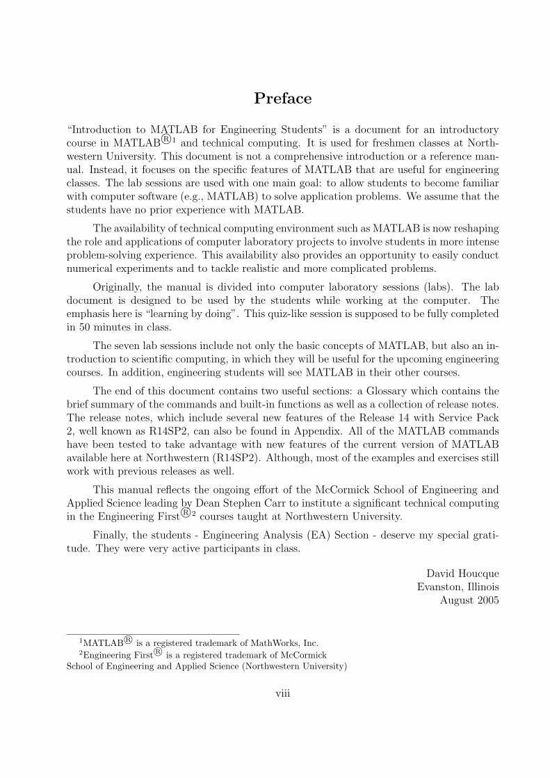
Preface

“Introduction to MATLAB for Engineering Students” is a document for an introductorycourse in MATLAB R©1 and technical computing. It is used for freshmen classes at North-western University. This document is not a comprehensive introduction or a reference man-ual. Instead, it focuses on the specific features of MATLAB that are useful for engineeringclasses. The lab sessions are used with one main goal: to allow students to become familiarwith computer software (e.g., MATLAB) to solve application problems. We assume that thestudents have no prior experience with MATLAB.

The availability of technical computing environment such as MATLAB is now reshapingthe role and applications of computer laboratory projects to involve students in more intenseproblem-solving experience. This availability also provides an opportunity to easily conductnumerical experiments and to tackle realistic and more complicated problems.

Originally, the manual is divided into computer laboratory sessions (labs). The labdocument is designed to be used by the students while working at the computer. Theemphasis here is “learning by doing”. This quiz-like session is supposed to be fully completedin 50 minutes in class.

The seven lab sessions include not only the basic concepts of MATLAB, but also an in-troduction to scientific computing, in which they will be useful for the upcoming engineeringcourses. In addition, engineering students will see MATLAB in their other courses.

The end of this document contains two useful sections: a Glossary which contains thebrief summary of the commands and built-in functions as well as a collection of release notes.The release notes, which include several new features of the Release 14 with Service Pack2, well known as R14SP2, can also be found in Appendix. All of the MATLAB commandshave been tested to take advantage with new features of the current version of MATLABavailable here at Northwestern (R14SP2). Although, most of the examples and exercises stillwork with previous releases as well.

This manual reflects the ongoing effort of the McCormick School of Engineering andApplied Science leading by Dean Stephen Carr to institute a significant technical computingin the Engineering First R©2 courses taught at Northwestern University.

Finally, the students - Engineering Analysis (EA) Section - deserve my special grati-tude. They were very active participants in class.

David HoucqueEvanston, Illinois

August 2005

1MATLAB R© is a registered trademark of MathWorks, Inc.2Engineering First R© is a registered trademark of McCormick

School of Engineering and Applied Science (Northwestern University)

viii

Acknowledgements

I would like to thank Dean Stephen Carr for his constant support. I am grateful to a numberof people who offered helpful advice and comments. I want to thank the EA1 instructors(Fall Quarter 2004), in particular Randy Freeman, Jorge Nocedal, and Allen Taflove fortheir helpful reviews on some specific parts of the document. I also want to thank MalcombMacIver, EA3 Honors instructor (Spring 2005) for helping me to better understand theanimation of system dynamics using MATLAB. I am particularly indebted to the manystudents (340 or so) who have used these materials, and have communicated their commentsand suggestions. Finally, I want to thank IT personnel for helping setting up the classes andother computer related work: Rebecca Swierz, Jesse Becker, Rick Mazec, Alan Wolff, KenKalan, Mike Vilches, and Daniel Lee.

About the author

David Houcque has more than 25 years’ experience in the modeling and simulation of struc-tures and solid continua including 14 years in industry. In industry, he has been working asR&D engineer in the fields of nuclear engineering, oil rig platform offshore design, oil reser-voir engineering, and steel industry. All of these include working in different internationalenvironments: Germany, France, Norway, and United Arab Emirates. Among other things,he has a combined background experience: scientific computing and engineering expertise.He earned his academic degrees from Europe and the United States.

Here at Northwestern University, he is working under the supervision of Professor BrianMoran, a world-renowned expert in fracture mechanics, to investigate the integrity assess-ment of the aging highway bridges under severe operating conditions and corrosion.

ix

Chapter 1

Tutorial lessons 1

1.1 Introduction

The tutorials are independent of the rest of the document. The primarily objective is to helpyou learn quickly the first steps. The emphasis here is “learning by doing”. Therefore, thebest way to learn is by trying it yourself. Working through the examples will give you a feelfor the way that MATLAB operates. In this introduction we will describe how MATLABhandles simple numerical expressions and mathematical formulas.

The name MATLAB stands for MATrix LABoratory. MATLAB was written originallyto provide easy access to matrix software developed by the LINPACK (linear system package)and EISPACK (Eigen system package) projects.

MATLAB [1] is a high-performance language for technical computing. It integratescomputation, visualization, and programming environment. Furthermore, MATLAB is amodern programming language environment: it has sophisticated data structures, containsbuilt-in editing and debugging tools, and supports object-oriented programming. These factorsmake MATLAB an excellent tool for teaching and research.

MATLAB has many advantages compared to conventional computer languages (e.g.,C, FORTRAN) for solving technical problems. MATLAB is an interactive system whosebasic data element is an array that does not require dimensioning. The software packagehas been commercially available since 1984 and is now considered as a standard tool at mostuniversities and industries worldwide.

It has powerful built-in routines that enable a very wide variety of computations. Italso has easy to use graphics commands that make the visualization of results immediatelyavailable. Specific applications are collected in packages referred to as toolbox. There aretoolboxes for signal processing, symbolic computation, control theory, simulation, optimiza-tion, and several other fields of applied science and engineering.

In addition to the MATLAB documentation which is mostly available on-line, we would

1

recommend the following books: [2], [3], [4], [5], [6], [7], [8], and [9]. They are excellent intheir specific applications.

1.2 Basic features

As we mentioned earlier, the following tutorial lessons are designed to get you startedquickly in MATLAB. The lessons are intended to make you familiar with the basics ofMATLAB. We urge you to complete the exercises given at the end of each lesson.

1.3 A minimum MATLAB session

The goal of this minimum session (also called starting and exiting sessions) is to learn thefirst steps:

• How to log on

• Invoke MATLAB

• Do a few simple calculations

• How to quit MATLAB

1.3.1 Starting MATLAB

After logging into your account, you can enter MATLAB by double-clicking on the MATLABshortcut icon (MATLAB 7.0.4) on your Windows desktop. When you start MATLAB, aspecial window called the MATLAB desktop appears. The desktop is a window that containsother windows. The major tools within or accessible from the desktop are:

• The Command Window

• The Command History

• The Workspace

• The Current Directory

• The Help Browser

• The Start button

2

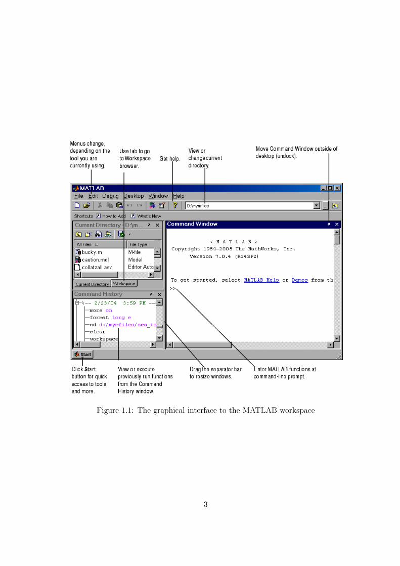
Figure 1.1: The graphical interface to the MATLAB workspace

3

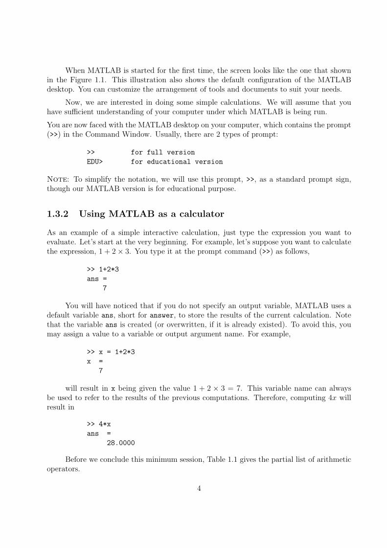
When MATLAB is started for the first time, the screen looks like the one that shownin the Figure 1.1. This illustration also shows the default configuration of the MATLABdesktop. You can customize the arrangement of tools and documents to suit your needs.

Now, we are interested in doing some simple calculations. We will assume that youhave sufficient understanding of your computer under which MATLAB is being run.

You are now faced with the MATLAB desktop on your computer, which contains the prompt(>>) in the Command Window. Usually, there are 2 types of prompt:

>> for full version

EDU> for educational version

Note: To simplify the notation, we will use this prompt, >>, as a standard prompt sign,though our MATLAB version is for educational purpose.

1.3.2 Using MATLAB as a calculator

As an example of a simple interactive calculation, just type the expression you want toevaluate. Let’s start at the very beginning. For example, let’s suppose you want to calculatethe expression, 1 + 2× 3. You type it at the prompt command (>>) as follows,

>> 1+2*3

ans =

7

You will have noticed that if you do not specify an output variable, MATLAB uses adefault variable ans, short for answer, to store the results of the current calculation. Notethat the variable ans is created (or overwritten, if it is already existed). To avoid this, youmay assign a value to a variable or output argument name. For example,

>> x = 1+2*3

x =

7

will result in x being given the value 1 + 2 × 3 = 7. This variable name can alwaysbe used to refer to the results of the previous computations. Therefore, computing 4x willresult in

>> 4*x

ans =

28.0000

Before we conclude this minimum session, Table 1.1 gives the partial list of arithmeticoperators.

4

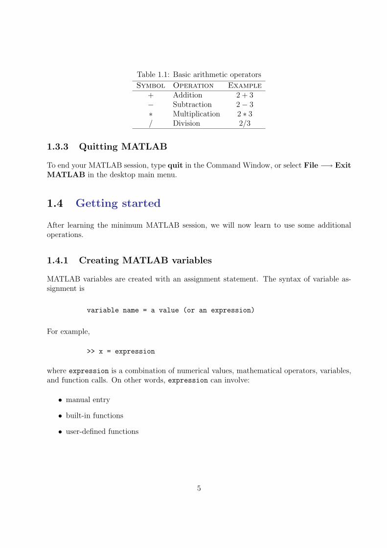
Table 1.1: Basic arithmetic operators

Symbol Operation Example+ Addition 2 + 3− Subtraction 2− 3∗ Multiplication 2 ∗ 3/ Division 2/3

1.3.3 Quitting MATLAB

To end your MATLAB session, type quit in the Command Window, or select File −→ ExitMATLAB in the desktop main menu.

1.4 Getting started

After learning the minimum MATLAB session, we will now learn to use some additionaloperations.

1.4.1 Creating MATLAB variables

MATLAB variables are created with an assignment statement. The syntax of variable as-signment is

variable name = a value (or an expression)

For example,

>> x = expression

where expression is a combination of numerical values, mathematical operators, variables,and function calls. On other words, expression can involve:

• manual entry

• built-in functions

• user-defined functions

5

1.4.2 Overwriting variable

Once a variable has been created, it can be reassigned. In addition, if you do not wish tosee the intermediate results, you can suppress the numerical output by putting a semicolon(;) at the end of the line. Then the sequence of commands looks like this:

>> t = 5;

>> t = t+1

t =

6

1.4.3 Error messages

If we enter an expression incorrectly, MATLAB will return an error message. For example,in the following, we left out the multiplication sign, *, in the following expression

>> x = 10;

>> 5x

??? 5x

|

Error: Unexpected MATLAB expression.

1.4.4 Making corrections

To make corrections, we can, of course retype the expressions. But if the expression islengthy, we make more mistakes by typing a second time. A previously typed commandcan be recalled with the up-arrow key ↑. When the command is displayed at the commandprompt, it can be modified if needed and executed.

1.4.5 Controlling the hierarchy of operations or precedence

Let’s consider the previous arithmetic operation, but now we will include parentheses. Forexample, 1 + 2× 3 will become (1 + 2)× 3

>> (1+2)*3

ans =

9

and, from previous example

6

>> 1+2*3

ans =

7

By adding parentheses, these two expressions give different results: 9 and 7.

The order in which MATLAB performs arithmetic operations is exactly that taughtin high school algebra courses. Exponentiations are done first, followed by multiplicationsand divisions, and finally by additions and subtractions. However, the standard order ofprecedence of arithmetic operations can be changed by inserting parentheses. For example,the result of 1+2×3 is quite different than the similar expression with parentheses (1+2)×3.The results are 7 and 9 respectively. Parentheses can always be used to overrule priority,and their use is recommended in some complex expressions to avoid ambiguity.

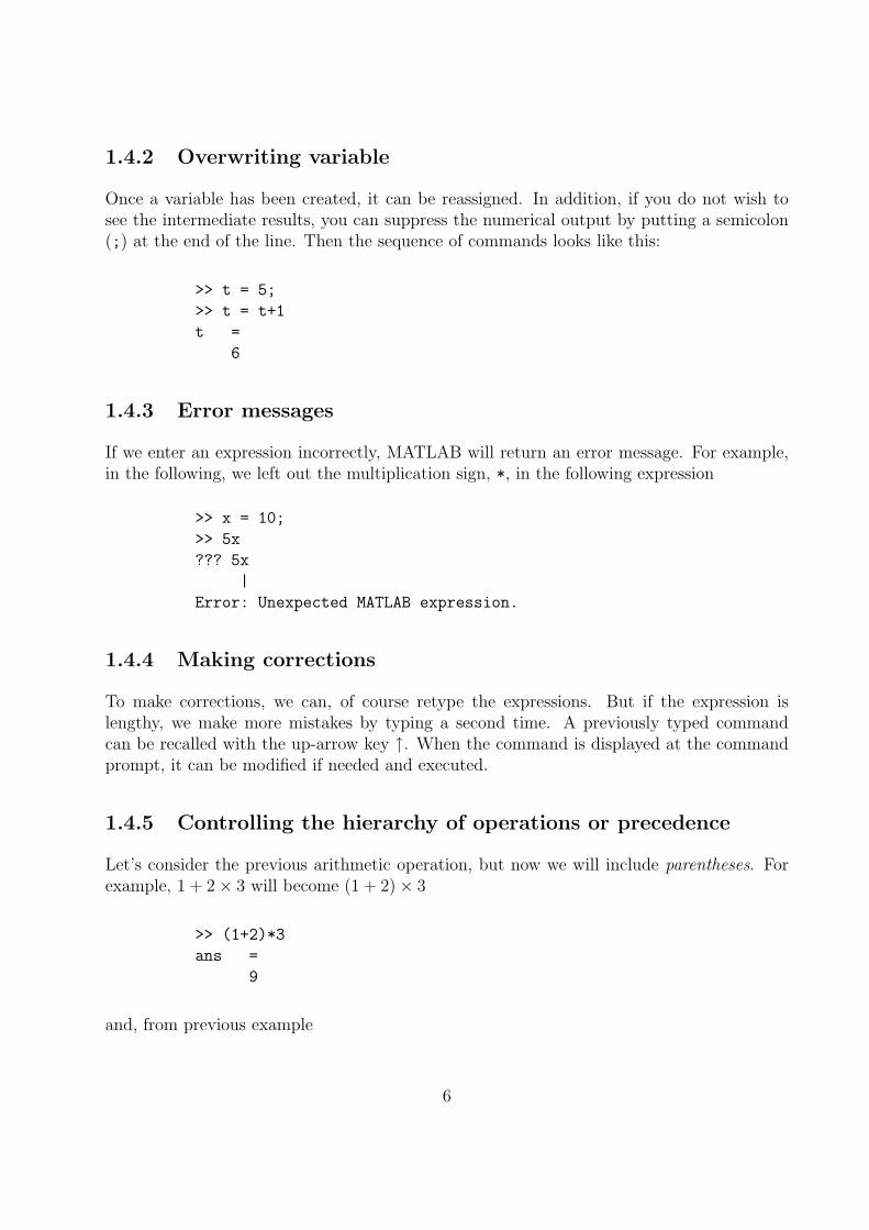
Therefore, to make the evaluation of expressions unambiguous, MATLAB has estab-lished a series of rules. The order in which the arithmetic operations are evaluated is givenin Table 1.2.

Table 1.2: Hierarchy of arithmetic operations

Precedence Mathematical operationsFirst The contents of all parentheses are evaluated first, starting

from the innermost parentheses and working outward.Second All exponentials are evaluated, working from left to rightThird All multiplications and divisions are evaluated, working

from left to rightFourth All additions and subtractions are evaluated, starting

from left to right

MATLAB arithmetic operators obey the same precedence rules as those in most com-puter programs. For operators of equal precedence, evaluation is from left to right. Now,consider another example:

1

2 + 32+

4

5× 6

7

In MATLAB, it becomes

>> 1/(2+3^2)+4/5*6/7

ans =

0.7766

or, if parentheses are missing,

7

>> 1/2+3^2+4/5*6/7

ans =

10.1857

So here what we get: two different results. Therefore, we want to emphasize theimportance of precedence rule in order to avoid ambiguity.

1.4.6 Controlling the appearance of floating point number

MATLAB by default displays only 4 decimals in the result of the calculations, for example−163.6667, as shown in above examples. However, MATLAB does numerical calculationsin double precision, which is 15 digits. The command format controls how the results ofcomputations are displayed. Here are some examples of the different formats together withthe resulting outputs.

>> format short

>> x=-163.6667

If we want to see all 15 digits, we use the command format long

>> format long

>> x= -1.636666666666667e+002

To return to the standard format, enter format short, or simply format.

There are several other formats. For more details, see the MATLAB documentation,or type help format.

Note - Up to now, we have let MATLAB repeat everything that we enter at theprompt (>>). Sometimes this is not quite useful, in particular when the output is pages enlength. To prevent MATLAB from echoing what we type, simply enter a semicolon (;) atthe end of the command. For example,

>> x=-163.6667;

and then ask about the value of x by typing,

>> x

x =

-163.6667

8

1.4.7 Managing the workspace

The contents of the workspace persist between the executions of separate commands. There-fore, it is possible for the results of one problem to have an effect on the next one. To avoidthis possibility, it is a good idea to issue a clear command at the start of each new inde-pendent calculation.

>> clear

The command clear or clear all removes all variables from the workspace. Thisfrees up system memory. In order to display a list of the variables currently in the memory,type

>> who

while, whos will give more details which include size, space allocation, and class of thevariables.

1.4.8 Keeping track of your work session

It is possible to keep track of everything done during a MATLAB session with the diary

command.

>> diary

or give a name to a created file,

>> diary FileName

where FileName could be any arbitrary name you choose.

The function diary is useful if you want to save a complete MATLAB session. Theysave all input and output as they appear in the MATLAB window. When you want to stopthe recording, enter diary off. If you want to start recording again, enter diary on. Thefile that is created is a simple text file. It can be opened by an editor or a word processingprogram and edited to remove extraneous material, or to add your comments. You canuse the function type to view the diary file or you can edit in a text editor or print. Thiscommand is useful, for example in the process of preparing a homework or lab submission.

9

1.4.9 Entering multiple statements per line

It is possible to enter multiple statements per line. Use commas (,) or semicolons (;) toenter more than one statement at once. Commas (,) allow multiple statements per linewithout suppressing output.

>> a=7; b=cos(a), c=cosh(a)

b =

0.6570

c =

548.3170

1.4.10 Miscellaneous commands

Here are few additional useful commands:

• To clear the Command Window, type clc

• To abort a MATLAB computation, type ctrl-c

• To continue a line, type . . .

1.4.11 Getting help

To view the online documentation, select MATLAB Help from Help menu or MATLAB Helpdirectly in the Command Window. The preferred method is to use the Help Browser. TheHelp Browser can be started by selecting the ? icon from the desktop toolbar. On the otherhand, information about any command is available by typing

>> help Command

Another way to get help is to use the lookfor command. The lookfor command differsfrom the help command. The help command searches for an exact function name match,while the lookfor command searches the quick summary information in each function fora match. For example, suppose that we were looking for a function to take the inverse ofa matrix. Since MATLAB does not have a function named inverse, the command help

inverse will produce nothing. On the other hand, the command lookfor inverse willproduce detailed information, which includes the function of interest, inv.

>> lookfor inverse

10

Note - At this particular time of our study, it is important to emphasize one main point.Because MATLAB is a huge program; it is impossible to cover all the details of each functionone by one. However, we will give you information how to get help. Here are some examples:

• Use on-line help to request info on a specific function

>> help sqrt

• In the current version (MATLAB version 7), the doc function opens the on-line versionof the help manual. This is very helpful for more complex commands.

>> doc plot

• Use lookfor to find functions by keywords. The general form is

>> lookfor FunctionName

1.5 Exercises

Note: Due to the teaching class during this Fall 2005, the problems are temporarily removedfrom this section.

11

Chapter 2

Tutorial lessons 2

2.1 Mathematical functions

MATLAB offers many predefined mathematical functions for technical computing whichcontains a large set of mathematical functions.

Typing help elfun and help specfun calls up full lists of elementary and specialfunctions respectively.

There is a long list of mathematical functions that are built into MATLAB. Thesefunctions are called built-ins. Many standard mathematical functions, such as sin(x), cos(x),tan(x), ex, ln(x), are evaluated by the functions sin, cos, tan, exp, and log respectively inMATLAB.

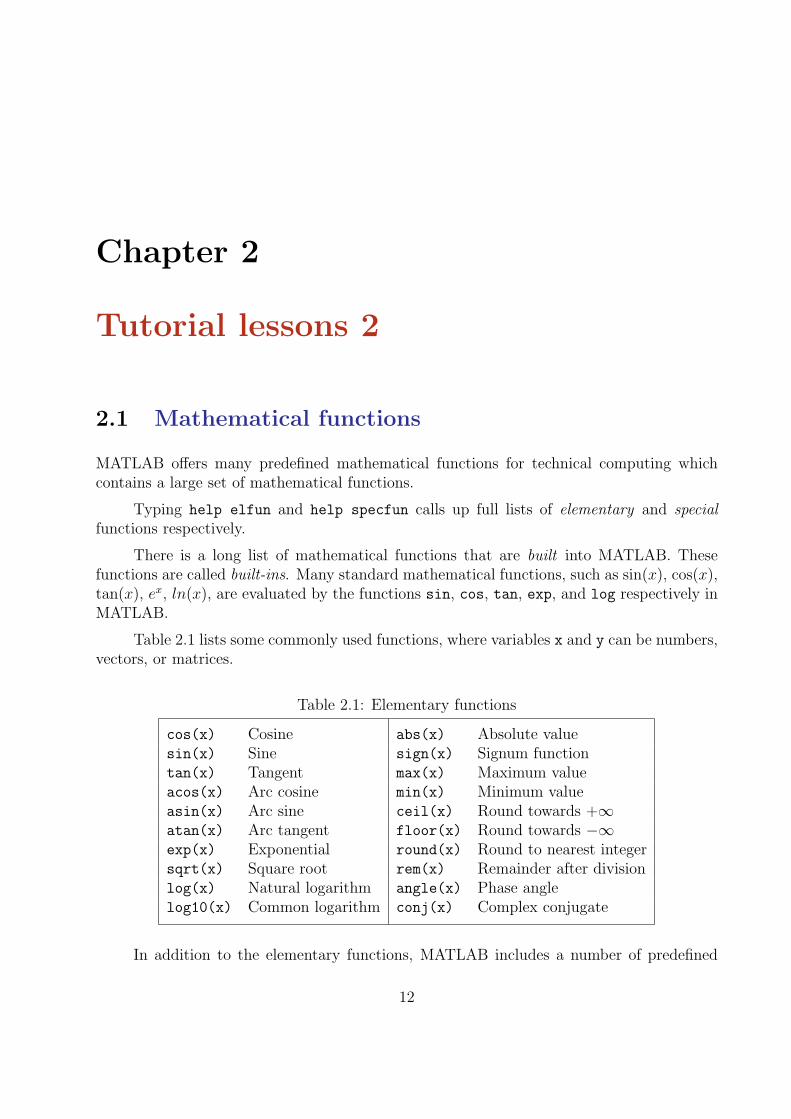
Table 2.1 lists some commonly used functions, where variables x and y can be numbers,vectors, or matrices.

Table 2.1: Elementary functions

cos(x) Cosine abs(x) Absolute valuesin(x) Sine sign(x) Signum functiontan(x) Tangent max(x) Maximum valueacos(x) Arc cosine min(x) Minimum valueasin(x) Arc sine ceil(x) Round towards +∞atan(x) Arc tangent floor(x) Round towards −∞exp(x) Exponential round(x) Round to nearest integersqrt(x) Square root rem(x) Remainder after divisionlog(x) Natural logarithm angle(x) Phase anglelog10(x) Common logarithm conj(x) Complex conjugate

In addition to the elementary functions, MATLAB includes a number of predefined

12

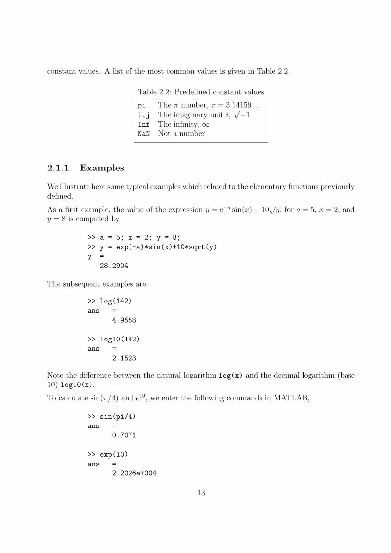
constant values. A list of the most common values is given in Table 2.2.

Table 2.2: Predefined constant values

pi The π number, π = 3.14159 . . .i,j The imaginary unit i,

√−1Inf The infinity, ∞NaN Not a number

2.1.1 Examples

We illustrate here some typical examples which related to the elementary functions previouslydefined.

As a first example, the value of the expression y = e−a sin(x) + 10√

y, for a = 5, x = 2, andy = 8 is computed by

>> a = 5; x = 2; y = 8;

>> y = exp(-a)*sin(x)+10*sqrt(y)

y =

28.2904

The subsequent examples are

>> log(142)

ans =

4.9558

>> log10(142)

ans =

2.1523

Note the difference between the natural logarithm log(x) and the decimal logarithm (base10) log10(x).

To calculate sin(π/4) and e10, we enter the following commands in MATLAB,

>> sin(pi/4)

ans =

0.7071

>> exp(10)

ans =

2.2026e+004

13

Notes:

• Only use built-in functions on the right hand side of an expression. Reassigning thevalue to a built-in function can create problems.

• There are some exceptions. For example, i and j are pre-assigned to√−1. However,

one or both of i or j are often used as loop indices.

• To avoid any possible confusion, it is suggested to use instead ii or jj as loop indices.

2.2 Basic plotting

2.2.1 overview

MATLAB has an excellent set of graphic tools. Plotting a given data set or the resultsof computation is possible with very few commands. You are highly encouraged to plotmathematical functions and results of analysis as often as possible. Trying to understandmathematical equations with graphics is an enjoyable and very efficient way of learning math-ematics. Being able to plot mathematical functions and data freely is the most importantstep, and this section is written to assist you to do just that.

2.2.2 Creating simple plots

The basic MATLAB graphing procedure, for example in 2D, is to take a vector of x-coordinates, x = (x1, . . . , xN), and a vector of y-coordinates, y = (y1, . . . , yN), locate thepoints (xi, yi), with i = 1, 2, . . . , n and then join them by straight lines. You need to preparex and y in an identical array form; namely, x and y are both row arrays or column arrays ofthe same length.

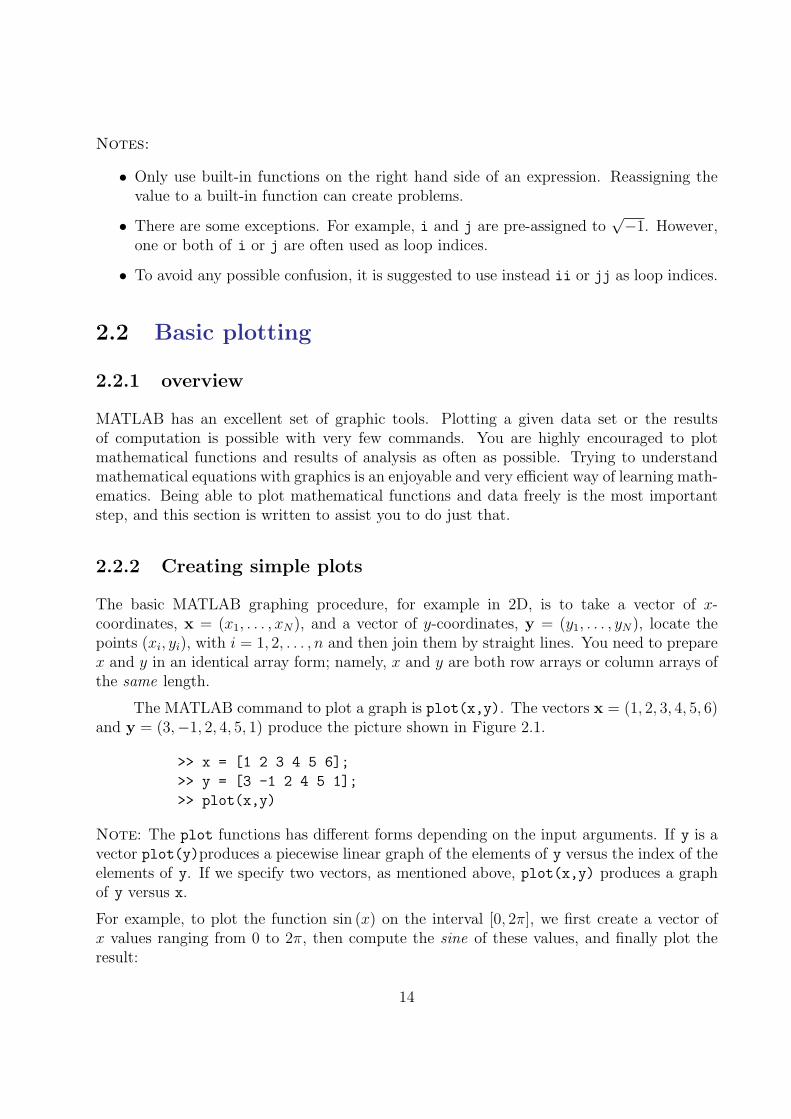
The MATLAB command to plot a graph is plot(x,y). The vectors x = (1, 2, 3, 4, 5, 6)and y = (3,−1, 2, 4, 5, 1) produce the picture shown in Figure 2.1.

>> x = [1 2 3 4 5 6];

>> y = [3 -1 2 4 5 1];

>> plot(x,y)

Note: The plot functions has different forms depending on the input arguments. If y is avector plot(y)produces a piecewise linear graph of the elements of y versus the index of theelements of y. If we specify two vectors, as mentioned above, plot(x,y) produces a graphof y versus x.

For example, to plot the function sin (x) on the interval [0, 2π], we first create a vector ofx values ranging from 0 to 2π, then compute the sine of these values, and finally plot theresult:

14

1 2 3 4 5 6−1

0

1

2

3

4

5

Figure 2.1: Plot for the vectors x and y

>> x = 0:pi/100:2*pi;

>> y = sin(x);

>> plot(x,y)

Notes:

• 0:pi/100:2*pi yields a vector that

– starts at 0,

– takes steps (or increments) of π/100,

– stops when 2π is reached.

• If you omit the increment, MATLAB automatically increments by 1.

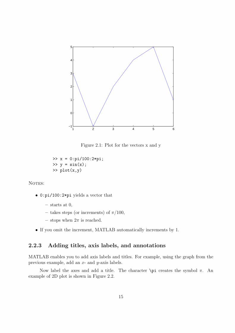
2.2.3 Adding titles, axis labels, and annotations

MATLAB enables you to add axis labels and titles. For example, using the graph from theprevious example, add an x- and y-axis labels.

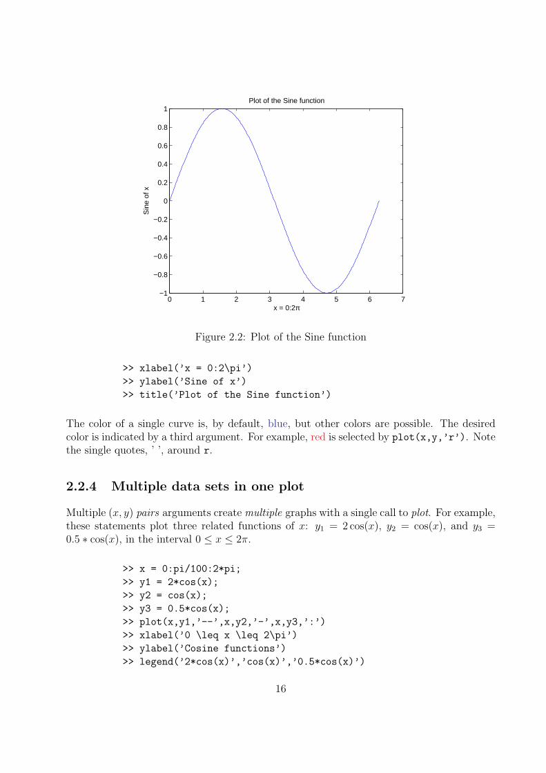
Now label the axes and add a title. The character \pi creates the symbol π. Anexample of 2D plot is shown in Figure 2.2.

15

0 1 2 3 4 5 6 7−1

−0.8

−0.6

−0.4

−0.2

0

0.2

0.4

0.6

0.8

1

x = 0:2π

Sin

e of

x

Plot of the Sine function

Figure 2.2: Plot of the Sine function

>> xlabel(’x = 0:2\pi’)

>> ylabel(’Sine of x’)

>> title(’Plot of the Sine function’)

The color of a single curve is, by default, blue, but other colors are possible. The desiredcolor is indicated by a third argument. For example, red is selected by plot(x,y,’r’). Notethe single quotes, ’ ’, around r.

2.2.4 Multiple data sets in one plot

Multiple (x, y) pairs arguments create multiple graphs with a single call to plot. For example,these statements plot three related functions of x: y1 = 2 cos(x), y2 = cos(x), and y3 =0.5 ∗ cos(x), in the interval 0 ≤ x ≤ 2π.

>> x = 0:pi/100:2*pi;

>> y1 = 2*cos(x);

>> y2 = cos(x);

>> y3 = 0.5*cos(x);

>> plot(x,y1,’--’,x,y2,’-’,x,y3,’:’)

>> xlabel(’0 \leq x \leq 2\pi’)

>> ylabel(’Cosine functions’)

>> legend(’2*cos(x)’,’cos(x)’,’0.5*cos(x)’)

16

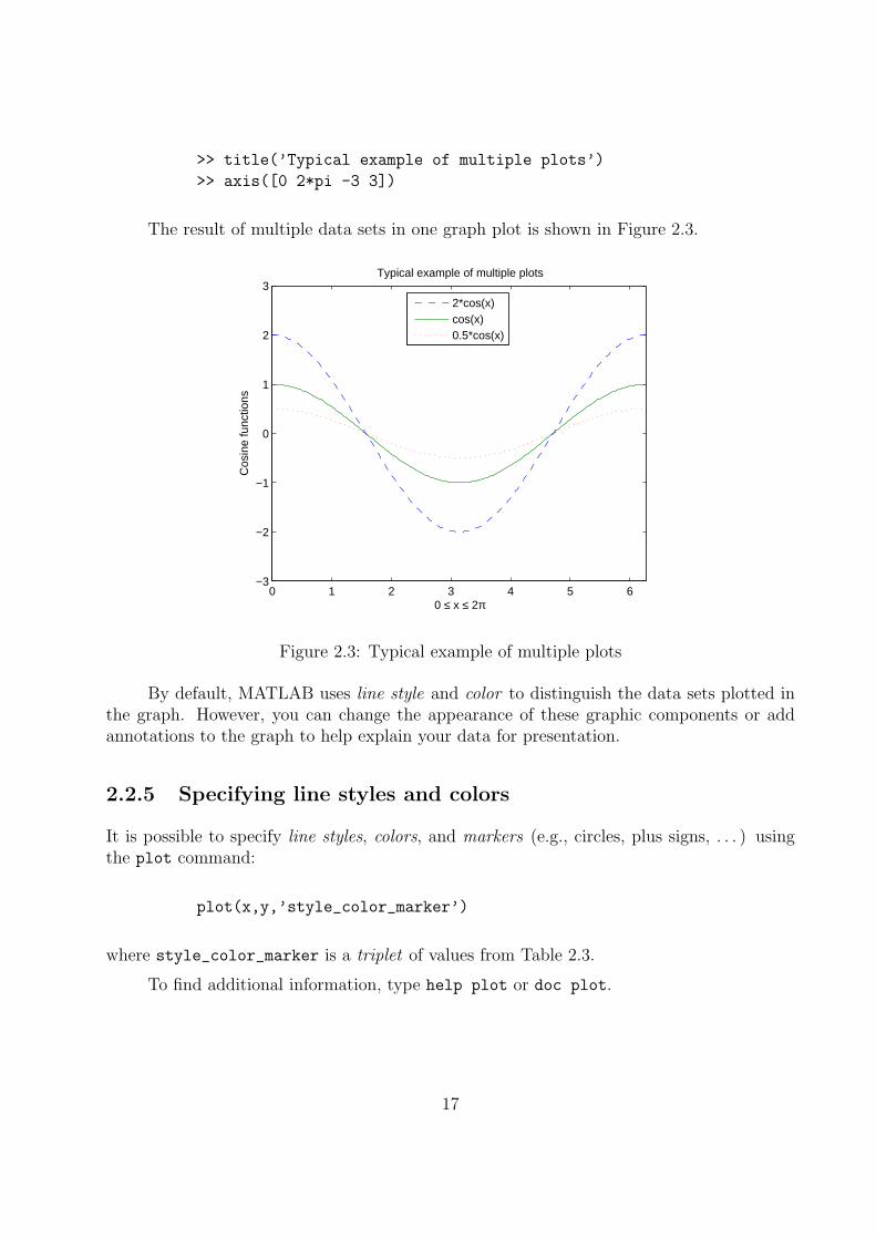
>> title(’Typical example of multiple plots’)

>> axis([0 2*pi -3 3])

The result of multiple data sets in one graph plot is shown in Figure 2.3.

0 1 2 3 4 5 6−3

−2

−1

0

1

2

3

0 ≤ x ≤ 2π

Cos

ine

func

tions

Typical example of multiple plots

2*cos(x)cos(x)0.5*cos(x)

Figure 2.3: Typical example of multiple plots

By default, MATLAB uses line style and color to distinguish the data sets plotted inthe graph. However, you can change the appearance of these graphic components or addannotations to the graph to help explain your data for presentation.

2.2.5 Specifying line styles and colors

It is possible to specify line styles, colors, and markers (e.g., circles, plus signs, . . . ) usingthe plot command:

plot(x,y,’style_color_marker’)

where style_color_marker is a triplet of values from Table 2.3.

To find additional information, type help plot or doc plot.

17

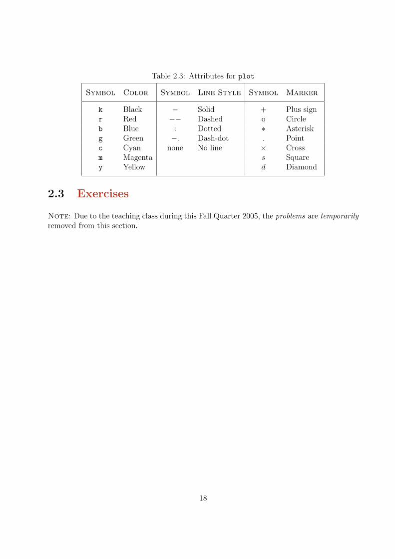
Table 2.3: Attributes for plot

Symbol Color Symbol Line Style Symbol Marker

k Black − Solid + Plus signr Red −− Dashed o Circleb Blue : Dotted ∗ Asteriskg Green −. Dash-dot . Pointc Cyan none No line × Crossm Magenta s Squarey Yellow d Diamond

2.3 Exercises

Note: Due to the teaching class during this Fall Quarter 2005, the problems are temporarilyremoved from this section.

18

Chapter 3

Matrix operations

3.1 Introduction

Matrices are the basic elements of the MATLAB environment. A matrix is a two-dimensionalarray consisting of m rows and n columns. Special cases are column vectors (n = 1) and rowvectors (m = 1).

In this section we will illustrate how to apply different operations on matrices. MAT-LAB supports two types of operations, known as matrix operations and array operations.The following topics are discussed: vectors and matrices in MATLAB, the inverse of a matrix,determinants, and matrix manipulation.

3.2 Matrix generation

Matrices are fundamental to MATLAB. Therefore, we need to become familiar with matrixgeneration and manipulation. Matrices can be generated in several ways.

3.2.1 Entering a vector

A vector is a special case of a matrix. The purpose of this section is to show how to createvectors and matrices in MATLAB. As discussed earlier, an array of dimension 1×n is calleda row vector. The elements of vectors in MATLAB are enclosed by square brackets and areseparated by spaces or by commas. For example,

>> v = [1 4 7 10 13]

v =

1 4 7 10 13

19

Similarly, column vectors are created in a similar way, however, semicolon (;) must separatethe components of a column vector,

>> w = [1;4;7;10;13]

w =

1

4

7

10

13

On the other hand, a row vector is converted to a column vector using the transpose operator.The transpose operation is denoted by an apostrophe or a single quote (’).

>> w = v’

w =

1

4

7

10

13

Thus, v(1) is the first element of vector v, v(2) its second element, and so forth.

Furthermore, to access blocks of elements, we use MATLAB’s colon notation. Forexample, to access the first three elements of v, we write,

>> v(1:3)

ans =

1 4 7

Or, all elements from the third through the last elements,

>> v(3,end)

ans =

7 10 13

where end signifies the last element in the vector. If v is a vector, writing

>> v(:)

produces a column vector, whereas writing

>> v(1:end)

produces a row vector.

20

3.2.2 Entering a matrix

A matrix is an array of numbers. To type a matrix into MATLAB you must

• begin with a square bracket, [

• separate elements in a row with spaces or commas (,)

• use a semicolon (;) to separate rows

• end the matrix with another square bracket, ].

Here is a typical example. To enter a matrix A, such as,

A =

1 2 34 5 67 8 9

(3.1)

we will enter each element of the matrix A as follow,

>> A = [1 2 3; 4 5 6; 7 8 9]

MATLAB then displays the 3× 3 matrix,

A =

1 2 3

4 5 6

7 8 9

Note that the use of semicolons (;) here is different from their use mentioned earlier tosuppress output or to write multiple commands in a single line.

Once we have entered the matrix, it is automatically stored and remembered in theworkspace. We can refer to it simply as matrix A. We can then view a particular element ina matrix by specifying its location. We write

>> A(2,1)

ans =

4

A(2,1) is an element located in the second row and first column. Its value is 4.

21

3.2.3 Matrix indexing

We select elements in a matrix just as we did for vectors, but now we need two indices.The element of row i and column j of the matrix A is denoted by A(i,j). Thus, A(i,j)in MATLAB refers to the element Aij of matrix A. The first index is the row number andthe second index is the column number. For example, A(1,3) is an element of first row andthird column. Here, A(1,3)=3.

Correcting any entry is easy through indexing. Here we substitute A(3,3)=9 by A(3,3)=0.The result is

>> A(3,3) = 0

A =

1 2 3

4 5 6

7 8 0

Single elements of a matrix are accessed as A(i,j), where i ≥ 1 and j ≥ 1 (zero or negativesubscripts are not supported in MATLAB).

3.2.4 Colon operator

The colon operator will prove very useful and understanding how it works is the key toefficient and convenient usage of MATLAB. It occurs in several different forms.

Often we must deal with matrices or vectors that are too large to enter one ele-ment at a time. For example, suppose we want to enter a vector x consisting of points(0, 0.1, 0.2, 0.3, · · · , 5). We can use the command

>> x = 0:0.1:5;

The row vector has 51 elements. The colon operator can also be used to pick out a certainrow or column. For example, the statement A(m:n,k:l specifies rows m to n and column kto l. Subscript expressions refer to portions of a matrix. For example,

>> A(2,:)

ans =

4 5 6

is the second row elements of A.

The colon operator can also be used to extract a sub-matrix from A.

>> A(:,2:3)

22

ans =

2 3

5 6

8 0

A(:,2:3) is a sub-matrix with the last two columns of A.

A row or a column of a matrix can be deleted by setting it to a null vector, [ ].

>> A(:,2)=[]

ans =

1 3

4 6

7 0

3.2.5 Linear spacing

On the other hand, there is a command to generate linearly spaced vectors: linspace. Itis similar to the colon operator (:), but gives direct control over the number of points. Forexample,

y = linspace(a,b)

generates a row vector y of 100 points linearly spaced between and including a and b.

y = linspace(a,b,n)

generates a row vector y of n points linearly spaced between and including a and b. This isuseful when we want to divide an interval into a number of subintervals of the same length.For example,

>> theta = linspace(0,2*pi,101)

divides the interval [0, 2π] into 100 equal subintervals, then creating a vector of 101 elements.

3.2.6 Creating a sub-matrix

To extract a submatrix B consisting of rows 2 and 3 and columns 1 and 2 of the matrix A,do the following

>> B = A([2 3],[1 2])

B =

4 5

7 8

23

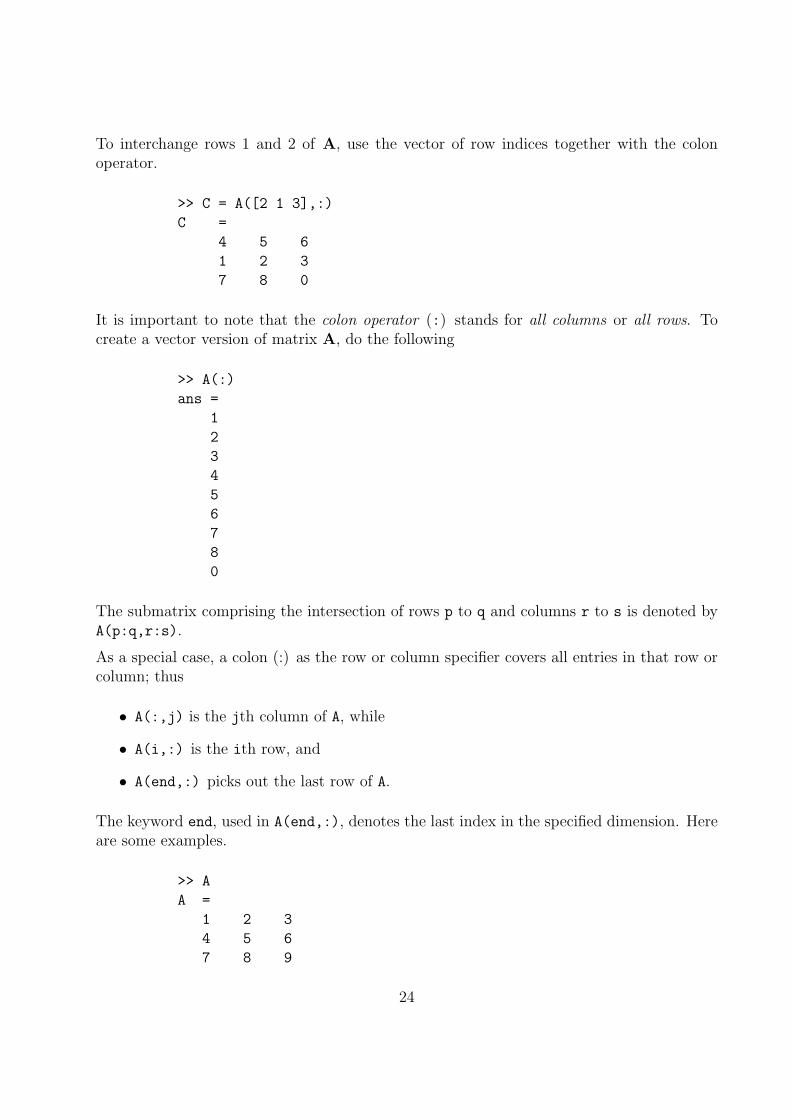
To interchange rows 1 and 2 of A, use the vector of row indices together with the colonoperator.

>> C = A([2 1 3],:)

C =

4 5 6

1 2 3

7 8 0

It is important to note that the colon operator (:) stands for all columns or all rows. Tocreate a vector version of matrix A, do the following

>> A(:)

ans =

1

2

3

4

5

6

7

8

0

The submatrix comprising the intersection of rows p to q and columns r to s is denoted byA(p:q,r:s).

As a special case, a colon (:) as the row or column specifier covers all entries in that row orcolumn; thus

• A(:,j) is the jth column of A, while

• A(i,:) is the ith row, and

• A(end,:) picks out the last row of A.

The keyword end, used in A(end,:), denotes the last index in the specified dimension. Hereare some examples.

>> A

A =

1 2 3

4 5 6

7 8 9

24

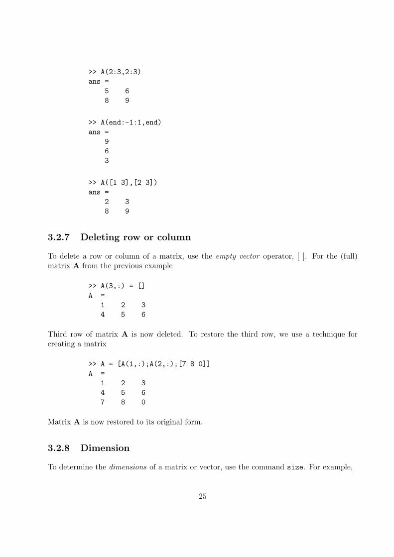
>> A(2:3,2:3)

ans =

5 6

8 9

>> A(end:-1:1,end)

ans =

9

6

3

>> A([1 3],[2 3])

ans =

2 3

8 9

3.2.7 Deleting row or column

To delete a row or column of a matrix, use the empty vector operator, [ ]. For the (full)matrix A from the previous example

>> A(3,:) = []

A =

1 2 3

4 5 6

Third row of matrix A is now deleted. To restore the third row, we use a technique forcreating a matrix

>> A = [A(1,:);A(2,:);[7 8 0]]

A =

1 2 3

4 5 6

7 8 0

Matrix A is now restored to its original form.

3.2.8 Dimension

To determine the dimensions of a matrix or vector, use the command size. For example,

25

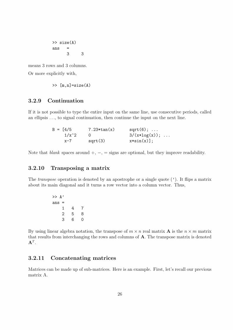
>> size(A)

ans =

3 3

means 3 rows and 3 columns.

Or more explicitly with,

>> [m,n]=size(A)

3.2.9 Continuation

If it is not possible to type the entire input on the same line, use consecutive periods, calledan ellipsis . . ., to signal continuation, then continue the input on the next line.

B = [4/5 7.23*tan(x) sqrt(6); ...

1/x^2 0 3/(x*log(x)); ...

x-7 sqrt(3) x*sin(x)];

Note that blank spaces around +, −, = signs are optional, but they improve readability.

3.2.10 Transposing a matrix

The transpose operation is denoted by an apostrophe or a single quote (’). It flips a matrixabout its main diagonal and it turns a row vector into a column vector. Thus,

>> A’

ans =

1 4 7

2 5 8

3 6 0

By using linear algebra notation, the transpose of m× n real matrix A is the n×m matrixthat results from interchanging the rows and columns of A. The transpose matrix is denotedAT .

3.2.11 Concatenating matrices

Matrices can be made up of sub-matrices. Here is an example. First, let’s recall our previousmatrix A.

26

A =

1 2 3

4 5 6

7 8 9

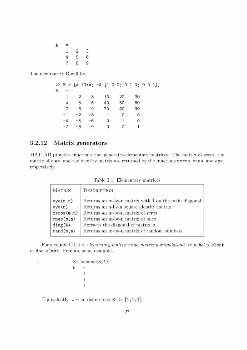
The new matrix B will be,

>> B = [A 10*A; -A [1 0 0; 0 1 0; 0 0 1]]

B =

1 2 3 10 20 30

4 5 6 40 50 60

7 8 9 70 80 90

-1 -2 -3 1 0 0

-4 -5 -6 0 1 0

-7 -8 -9 0 0 1

3.2.12 Matrix generators

MATLAB provides functions that generates elementary matrices. The matrix of zeros, thematrix of ones, and the identity matrix are returned by the functions zeros, ones, and eye,respectively.

Table 3.1: Elementary matrices

Matrix Description

eye(m,n) Returns an m-by-n matrix with 1 on the main diagonaleye(n) Returns an n-by-n square identity matrixzeros(m,n) Returns an m-by-n matrix of zerosones(m,n) Returns an m-by-n matrix of onesdiag(A) Extracts the diagonal of matrix Arand(m,n) Returns an m-by-n matrix of random numbers

For a complete list of elementary matrices and matrix manipulations, type help elmat

or doc elmat. Here are some examples:

1. >> b=ones(3,1)

b =

1

1

1

Equivalently, we can define b as >> b=[1;1;1]

27

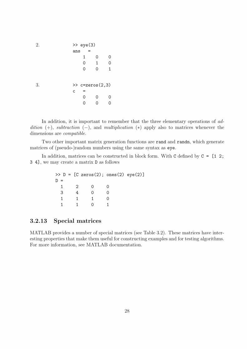
2. >> eye(3)

ans =

1 0 0

0 1 0

0 0 1

3. >> c=zeros(2,3)

c =

0 0 0

0 0 0

In addition, it is important to remember that the three elementary operations of ad-dition (+), subtraction (−), and multiplication (∗) apply also to matrices whenever thedimensions are compatible.

Two other important matrix generation functions are rand and randn, which generatematrices of (pseudo-)random numbers using the same syntax as eye.

In addition, matrices can be constructed in block form. With C defined by C = [1 2;

3 4], we may create a matrix D as follows

>> D = [C zeros(2); ones(2) eye(2)]

D =

1 2 0 0

3 4 0 0

1 1 1 0

1 1 0 1

3.2.13 Special matrices

MATLAB provides a number of special matrices (see Table 3.2). These matrices have inter-esting properties that make them useful for constructing examples and for testing algorithms.For more information, see MATLAB documentation.

28

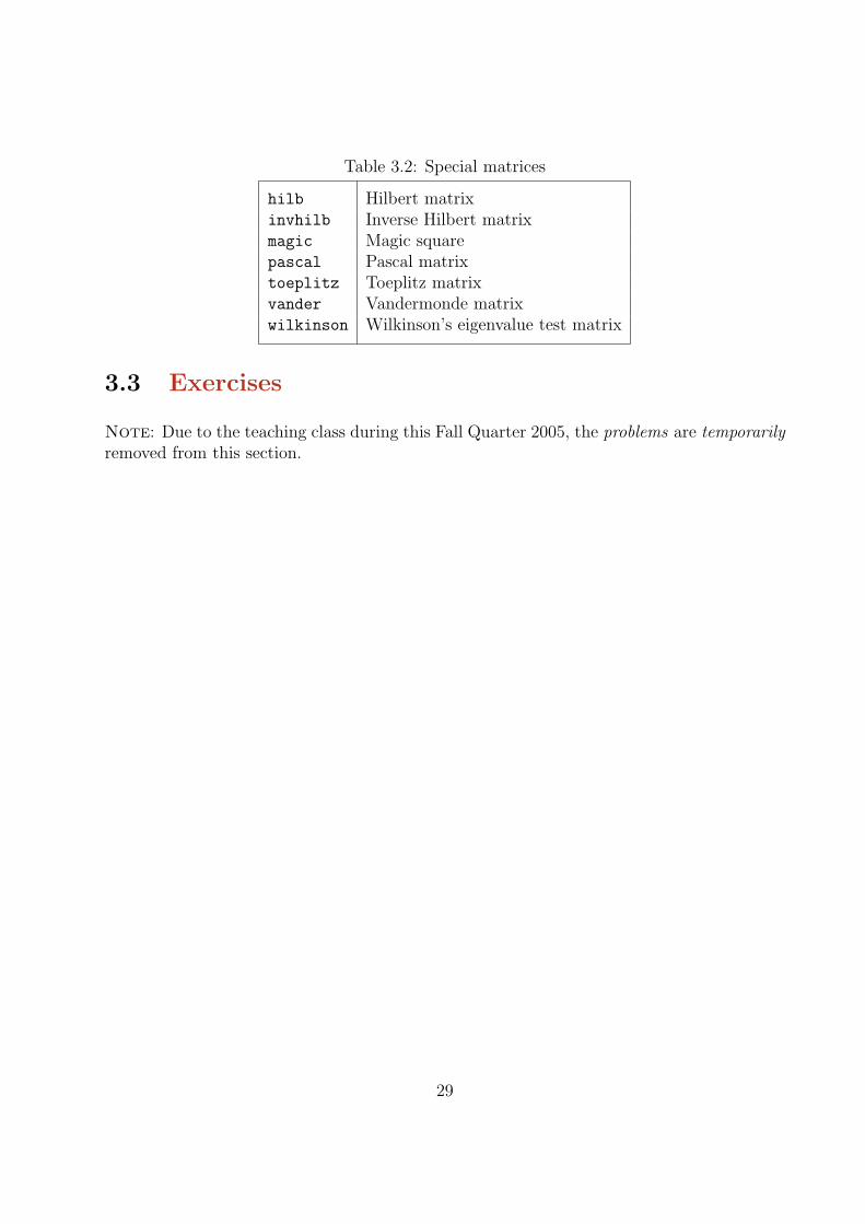
Table 3.2: Special matrices

hilb Hilbert matrixinvhilb Inverse Hilbert matrixmagic Magic squarepascal Pascal matrixtoeplitz Toeplitz matrixvander Vandermonde matrixwilkinson Wilkinson’s eigenvalue test matrix

3.3 Exercises

Note: Due to the teaching class during this Fall Quarter 2005, the problems are temporarilyremoved from this section.

29

Chapter 4

Array operations and Linearequations

MATLAB has two different types of arithmetic operations: matrix arithmetic operationsand array arithmetic operations.

4.1 Array operations

MATLAB has two different types of arithmetic operations: matrix arithmetic operationsand array arithmetic operations.

4.1.1 Matrix arithmetic operations

As we mentioned earlier, MATLAB allows arithmetic operations: +, −, ∗, and ˆ to becarried out on matrices. Thus,

A+B or B+A is valid if A and B are of the same sizeA*B is valid if A’s number of column equals B’s number of rowsAˆ2 is valid if A is square and equals A*Aα*A or A*α multiplies each element of A by α

4.1.2 Array arithmetic operations

On the other hand, array arithmetic operations or array operations for short are doneelement-by-element. The period character (.) distinguishes the array operations from thematrix operations. However, since the matrix and array operations are the same for addition

30

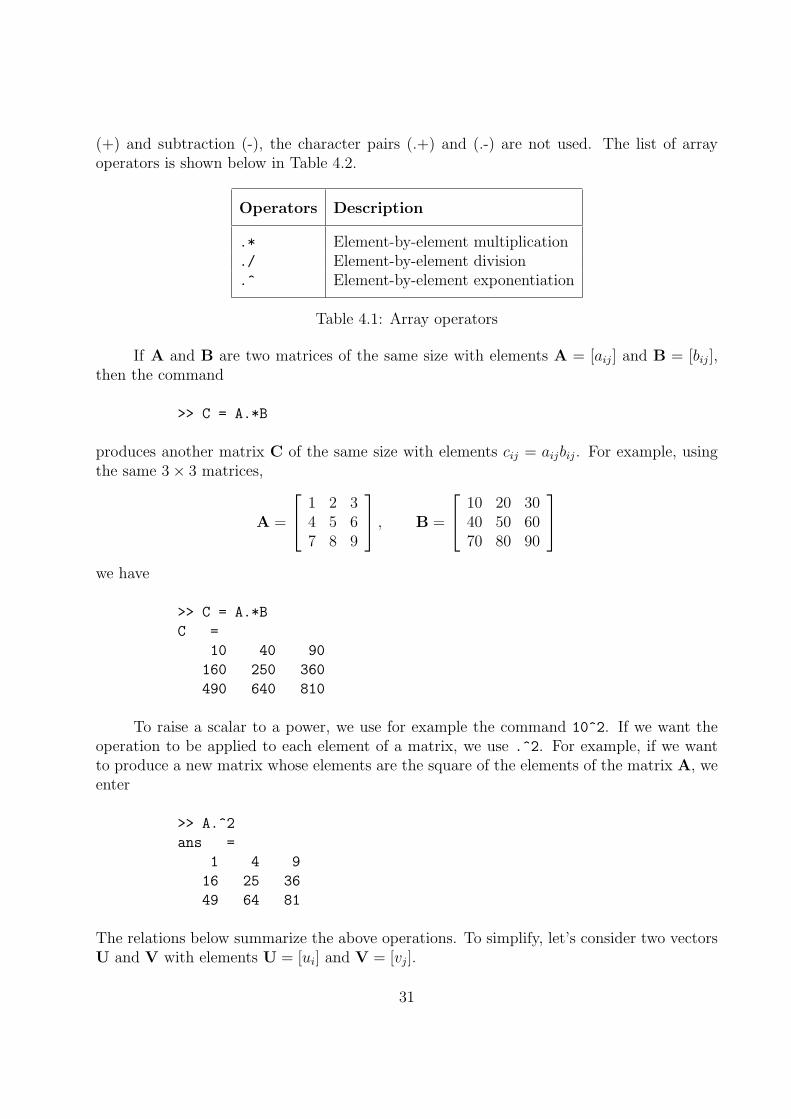
(+) and subtraction (-), the character pairs (.+) and (.-) are not used. The list of arrayoperators is shown below in Table 4.2.

Operators Description

.* Element-by-element multiplication

./ Element-by-element division

.^ Element-by-element exponentiation

Table 4.1: Array operators

If A and B are two matrices of the same size with elements A = [aij] and B = [bij],then the command

>> C = A.*B

produces another matrix C of the same size with elements cij = aijbij. For example, usingthe same 3× 3 matrices,

A =

1 2 34 5 67 8 9

, B =

10 20 3040 50 6070 80 90

we have

>> C = A.*B

C =

10 40 90

160 250 360

490 640 810

To raise a scalar to a power, we use for example the command 10^2. If we want theoperation to be applied to each element of a matrix, we use .^2. For example, if we wantto produce a new matrix whose elements are the square of the elements of the matrix A, weenter

>> A.^2

ans =

1 4 9

16 25 36

49 64 81

The relations below summarize the above operations. To simplify, let’s consider two vectorsU and V with elements U = [ui] and V = [vj].

31

U. ∗V produces [u1v1 u2v2 . . . unvn]U./V produces [u1/v1 u2/v2 . . . un/vn]U.ˆV produces [uv1

1 uv22 . . . uvn

n ]

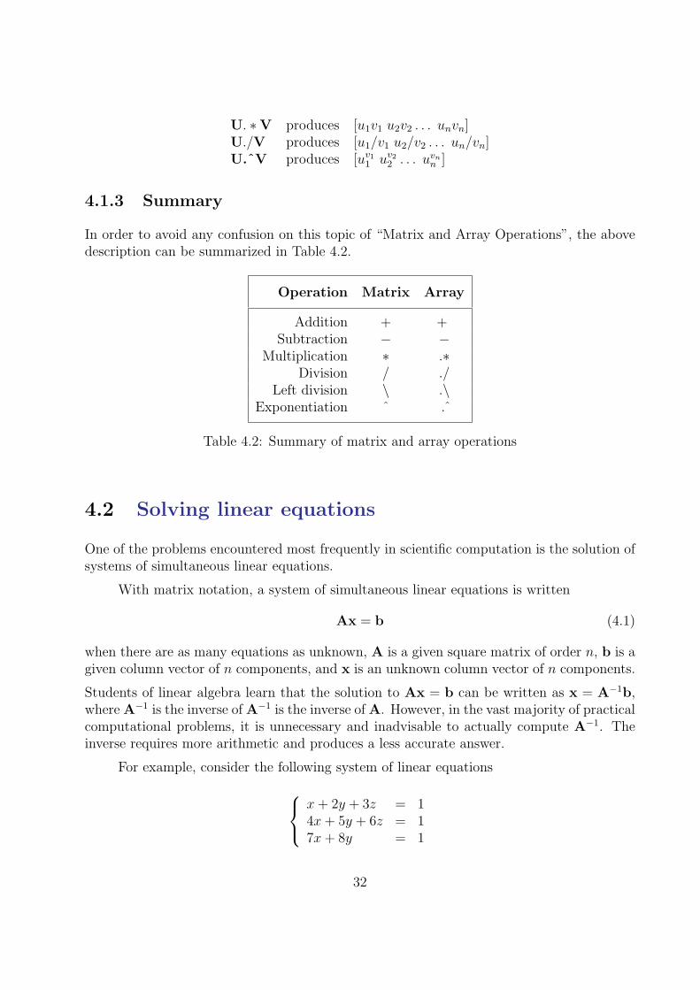
4.1.3 Summary

In order to avoid any confusion on this topic of “Matrix and Array Operations”, the abovedescription can be summarized in Table 4.2.

Operation Matrix Array

Addition + +Subtraction − −

Multiplication ∗ .∗Division / ./

Left division \ .\Exponentiation ˆ .̂

Table 4.2: Summary of matrix and array operations

4.2 Solving linear equations

One of the problems encountered most frequently in scientific computation is the solution ofsystems of simultaneous linear equations.

With matrix notation, a system of simultaneous linear equations is written

Ax = b (4.1)

when there are as many equations as unknown, A is a given square matrix of order n, b is agiven column vector of n components, and x is an unknown column vector of n components.

Students of linear algebra learn that the solution to Ax = b can be written as x = A−1b,where A−1 is the inverse of A−1 is the inverse of A. However, in the vast majority of practicalcomputational problems, it is unnecessary and inadvisable to actually compute A−1. Theinverse requires more arithmetic and produces a less accurate answer.

For example, consider the following system of linear equations

x + 2y + 3z = 14x + 5y + 6z = 17x + 8y = 1

32

The coefficient matrix A is

A =

1 2 34 5 67 8 9

and the vector b =

111

With matrix notation, a system of simultaneous linear equations is written

Ax = b (4.2)

This equation can be solved for x using linear algebra. The result is x = A−1b.

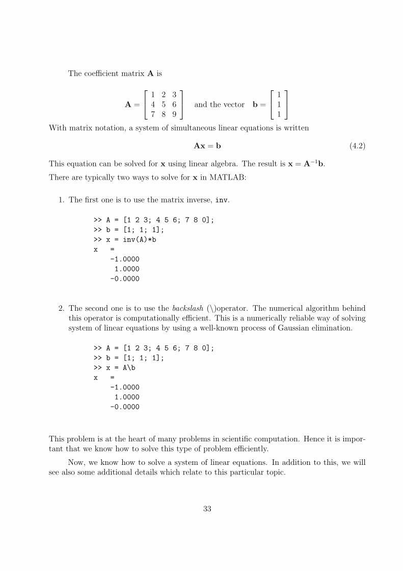
There are typically two ways to solve for x in MATLAB:

1. The first one is to use the matrix inverse, inv.

>> A = [1 2 3; 4 5 6; 7 8 0];

>> b = [1; 1; 1];

>> x = inv(A)*b

x =

-1.0000

1.0000

-0.0000

2. The second one is to use the backslash (\)operator. The numerical algorithm behindthis operator is computationally efficient. This is a numerically reliable way of solvingsystem of linear equations by using a well-known process of Gaussian elimination.

>> A = [1 2 3; 4 5 6; 7 8 0];

>> b = [1; 1; 1];

>> x = A\b

x =

-1.0000

1.0000

-0.0000

This problem is at the heart of many problems in scientific computation. Hence it is impor-tant that we know how to solve this type of problem efficiently.

Now, we know how to solve a system of linear equations. In addition to this, we willsee also some additional details which relate to this particular topic.

33

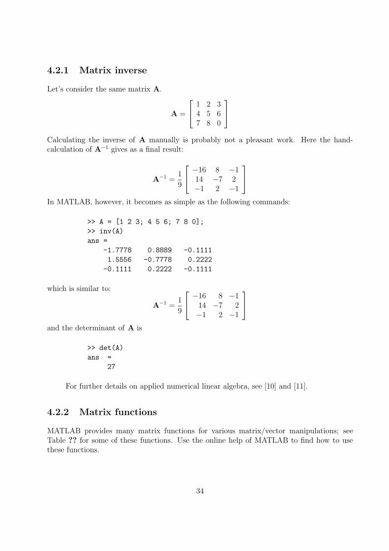
4.2.1 Matrix inverse

Let’s consider the same matrix A.

A =

1 2 34 5 67 8 0

Calculating the inverse of A manually is probably not a pleasant work. Here the hand-calculation of A−1 gives as a final result:

A−1 =1

9

−16 8 −114 −7 2−1 2 −1

In MATLAB, however, it becomes as simple as the following commands:

>> A = [1 2 3; 4 5 6; 7 8 0];

>> inv(A)

ans =

-1.7778 0.8889 -0.1111

1.5556 -0.7778 0.2222

-0.1111 0.2222 -0.1111

which is similar to:

A−1 =1

9

−16 8 −1

14 −7 2−1 2 −1

and the determinant of A is

>> det(A)

ans =

27

For further details on applied numerical linear algebra, see [10] and [11].

4.2.2 Matrix functions

MATLAB provides many matrix functions for various matrix/vector manipulations; seeTable ?? for some of these functions. Use the online help of MATLAB to find how to usethese functions.

34

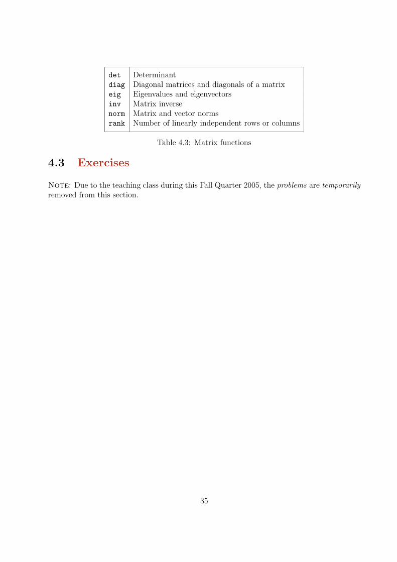
det Determinantdiag Diagonal matrices and diagonals of a matrixeig Eigenvalues and eigenvectorsinv Matrix inversenorm Matrix and vector normsrank Number of linearly independent rows or columns

Table 4.3: Matrix functions

4.3 Exercises

Note: Due to the teaching class during this Fall Quarter 2005, the problems are temporarilyremoved from this section.

35

Chapter 5

Introduction to M-File programming

5.1 Introduction

So far in this manual, all the commands were executed in the Command Window. Theproblem is that the commands entered in the Command Window cannot be saved andexecuted again for several times. Therefore, a different way of executing commands withMATLAB is

• first, to create a file with a list of commands,

• then, save it, and

• finally, run the file.

If needed, corrections or changes can be made to the commands in the file. The files thatare used for this purpose are called script files or scripts for short.

This section covers the following topics:

• M-File Scripts

• M-File Functions

5.2 M-File Scripts

A script file is an external file that contains a sequence of MATLAB statements. Scriptfiles have a filename extension .m and are often called M-files. M-files can be scripts thatsimply execute a series of MATLAB statements, or they can be functions that can acceptarguments and can produce one or more outputs.

36

5.2.1 Examples

Here are two simple scripts.

Example 1

Consider the system of equations:

x + 2y + 3z = 13x + 3y + 4z = 12x + 3y + 3z = 2

Find the solution x to the system of equations.

Solution:

• Use the MATLAB editor to create a file: File → New → M-file.

• Enter the following statements in the file:

A = [1 2 3; 3 3 4; 2 3 3];

b = [1; 1; 2];

x = A\b

• Save the file, for example, example1.m.

• Run the file, in the command line, by typing:

>> example1

x =

-0.5000

1.5000

-0.5000

When execution completes, the variables (A, b, and x) remain in the workspace. To see alisting of them, enter whos at the command prompt.

Note: The MATLAB editor is both a text editor specialized for creating M-files and agraphical MATLAB debugger. The MATLAB editor has numerous menus for tasks such assaving, viewing, and debugging. Because it performs some simple checks and also uses colorto differentiate between various elements of codes, this text editor is recommended as thetool of choice for writing and editing M-files. There is another way to open the editor:

37

>> edit

or

>> edit filename.m

to open filename.m.

Example 2

Plot the following cosine functions, y1 = 2 cos(x), y2 = cos(x), and y3 = 0.5 ∗ cos(x), in theinterval 0 ≤ x ≤ 2π. This example has been presented in previous Chapter. Here we putthe commands in a file.

• Create a file, example2.m, which contains the following commands:

x = 0:pi/100:2*pi;

y1 = 2*cos(x);

y2 = cos(x);

y3 = 0.5*cos(x);

plot(x,y1,’--’,x,y2,’-’,x,y3,’:’)

xlabel(’0 \leq x \leq 2\pi’)

ylabel(’Cosine functions’)

legend(’2*cos(x)’,’cos(x)’,’0.5*cos(x)’)

title(’Typical example of multiple plots’)

axis([0 2*pi -3 3])

• Run the file by typing example2 in the Command Window.

5.2.2 Script side-effects

All variables created in a script file are added to the workspace. This may have undesirableeffects, because:

• Variables already existing in the workspace may be overwritten.

• The execution of the script can be affected by the state variables in the workspace.

As a result, because scripts have some undesirable side effects, it is better to code anycomplicated applications using rather function M-file.

38

5.3 M-File functions

As mentioned earlier, functions are programs (or routines) that accept input arguments andreturn output arguments. Each M-file function (or function or M-file for short) has its ownarea of workspace, separated from the MATLAB base workspace.

5.3.1 Anatomy of a M-File function

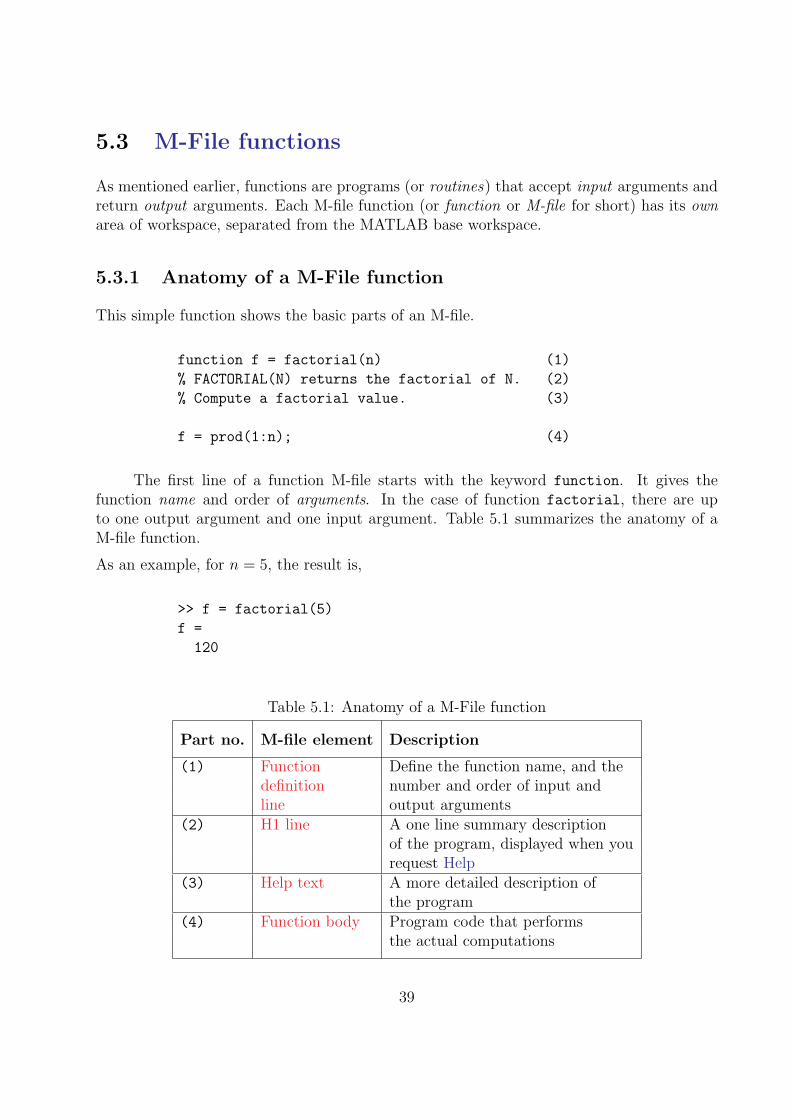
This simple function shows the basic parts of an M-file.

function f = factorial(n) (1)

% FACTORIAL(N) returns the factorial of N. (2)

% Compute a factorial value. (3)

f = prod(1:n); (4)

The first line of a function M-file starts with the keyword function. It gives thefunction name and order of arguments. In the case of function factorial, there are upto one output argument and one input argument. Table 5.1 summarizes the anatomy of aM-file function.

As an example, for n = 5, the result is,

>> f = factorial(5)

f =

120

Table 5.1: Anatomy of a M-File function

Part no. M-file element Description

(1) Function Define the function name, and thedefinition number and order of input andline output arguments

(2) H1 line A one line summary descriptionof the program, displayed when yourequest Help

(3) Help text A more detailed description ofthe program

(4) Function body Program code that performsthe actual computations

39

Both functions and scripts can have all of these parts, except for the function definitionline which applies to function only.

In addition, it is important to note that function name must begin with a letter, andmust be no longer than than the maximum of 63 characters. Furthermore, the name of thetext file that you save will consist of the function name with the extension .m. Thus, theabove example file would be factorial.m.

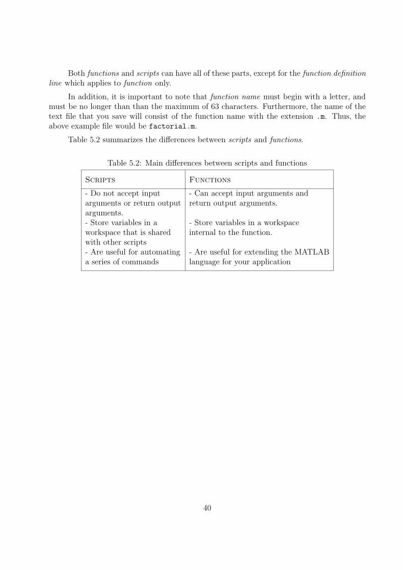
Table 5.2 summarizes the differences between scripts and functions.

Table 5.2: Main differences between scripts and functions

Scripts Functions

- Do not accept input - Can accept input arguments andarguments or return output return output arguments.arguments.- Store variables in a - Store variables in a workspaceworkspace that is shared internal to the function.with other scripts- Are useful for automating - Are useful for extending the MATLABa series of commands language for your application

40

5.3.2 Input and output arguments

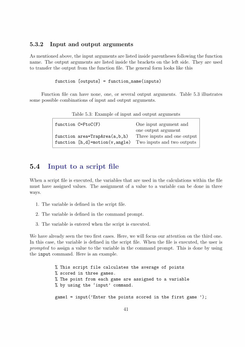
As mentioned above, the input arguments are listed inside parentheses following the functionname. The output arguments are listed inside the brackets on the left side. They are usedto transfer the output from the function file. The general form looks like this

function [outputs] = function_name(inputs)

Function file can have none, one, or several output arguments. Table 5.3 illustratessome possible combinations of input and output arguments.

Table 5.3: Example of input and output arguments

function C=FtoC(F) One input argument andone output argument

function area=TrapArea(a,b,h) Three inputs and one outputfunction [h,d]=motion(v,angle) Two inputs and two outputs

5.4 Input to a script file

When a script file is executed, the variables that are used in the calculations within the filemust have assigned values. The assignment of a value to a variable can be done in threeways.

1. The variable is defined in the script file.

2. The variable is defined in the command prompt.

3. The variable is entered when the script is executed.

We have already seen the two first cases. Here, we will focus our attention on the third one.In this case, the variable is defined in the script file. When the file is executed, the user isprompted to assign a value to the variable in the command prompt. This is done by usingthe input command. Here is an example.

% This script file calculates the average of points

% scored in three games.

% The point from each game are assigned to a variable

% by using the ‘input’ command.

game1 = input(’Enter the points scored in the first game ’);

41

game2 = input(’Enter the points scored in the second game ’);

game3 = input(’Enter the points scored in the third game ’);

average = (game1+game2+game3)/3

The following shows the command prompt when this script file (saved as example3) isexecuted.

>> example3

>> Enter the points scored in the first game 15

>> Enter the points scored in the second game 23

>> Enter the points scored in the third game 10

average =

16

The input command can also be used to assign string to a variable. For more infor-mation, see MATLAB documentation.

A typical example of M-file function programming can be found in a recent paper whichrelated to the solution of the ordinary differential equation (ODE) [12].

5.5 Output commands

As discussed before, MATLAB automatically generates a display when commands are exe-cuted. In addition to this automatic display, MATLAB has several commands that can beused to generate displays or outputs.

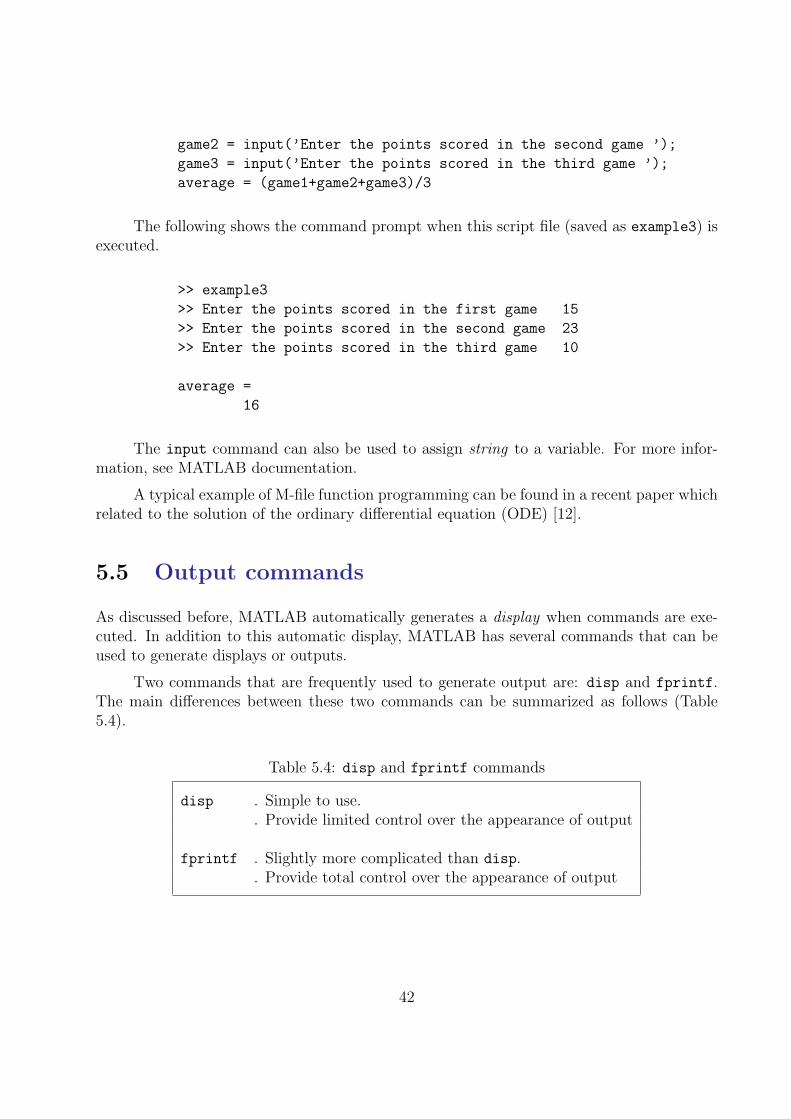
Two commands that are frequently used to generate output are: disp and fprintf.The main differences between these two commands can be summarized as follows (Table5.4).

Table 5.4: disp and fprintf commands

disp . Simple to use.. Provide limited control over the appearance of output

fprintf . Slightly more complicated than disp.. Provide total control over the appearance of output

42

5.5.1 Examples

The fprintf command

The fprintf command can be used to display output (text and data) on the screen or to saveit to a file. With this command, unlike the disp command, the output can be formatted.With many available options, the fprintf can be long and complicated. Recall the aboveexample.

% This script file calculates the average of points

% scored in three games.

% ’fprintf’ will be used for output.

game(1) = input(’Enter the points scored in the first game ’);

game(2) = input(’Enter the points scored in the second game ’);

game(3) = input(’Enter the points scored in the third game ’);

average = mean(game);

fprintf(’An average of %8.4f points was scored in 3 games ’,average)

>> example3

Enter the points scored in the first game 15

Enter the points scored in the second game 23

Enter the points scored in the third game 10

An average of 16.0000 points was scored in 3 games

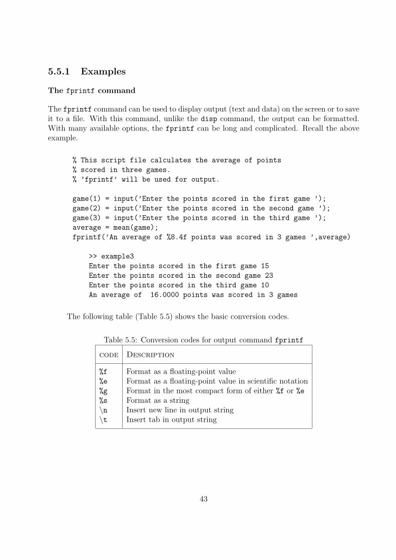
The following table (Table 5.5) shows the basic conversion codes.

Table 5.5: Conversion codes for output command fprintf

code Description

%f Format as a floating-point value%e Format as a floating-point value in scientific notation%g Format in the most compact form of either %f or %e%s Format as a string\n Insert new line in output string\t Insert tab in output string

43

5.6 Exercises

Note: Due to the teaching class during this Fall Quarter 2005, the problems are temporarilyremoved from this section.

44

Chapter 6

Control flow and operators

6.1 Introduction

MATLAB is also a programming language. Like other computer programming languages,MATLAB has some decision making structures for control of command execution. Thesedecision making or control flow structures include for loops, while loops, and if-else-end

constructions. Control flow structures are often used in script M-files and function M-files.

By creating a file with the extension .m, we can easily write and run programs. Wedo not need to compile the program since MATLAB is an interpretative (not compiled)language. MATLAB has thousand of functions, and you can add your own using m-files.

MATLAB provides several tools that can be used to control the flow of a program(script or function). In a simple program as shown in the previous Chapter, the commandsare executed one after the other. Here we introduce the flow control structure that makepossible to skip commands or to execute specific group of commands.

6.2 Control flow

MATLAB has four control flow structures: the if statement, the for loop, the while loop,and the switch statement.

6.2.1 The ‘‘if...end’’ structure

MATLAB supports the variants of “if” construct.

• if ... end

• if ... else ... end

45

• if ... elseif ... else ... end

The simplest form of the if statement is

if expression

statements

end

Here are some examples based on the familiar quadratic formula.

1. discr = b*b - 4*a*c;

if discr < 0

disp(’Warning: discriminant is negative, roots are

imaginary’);

end

2. discr = b*b - 4*a*c;

if discr < 0

disp(’Warning: discriminant is negative, roots are

imaginary’);

else

disp(’Roots are real, but may be repeated’)

end

3. discr = b*b - 4*a*c;

if discr < 0

disp(’Warning: discriminant is negative, roots are

imaginary’);

elseif discr == 0

disp(’Discriminant is zero, roots are repeated’)

else

disp(’Roots are real’)

end

It should be noted that:

• elseif has no space between else and if (one word)

• no semicolon (;) is needed at the end of lines containing if, else, end

• indentation of if block is not required, but facilitate the reading.

• the end statement is required

46

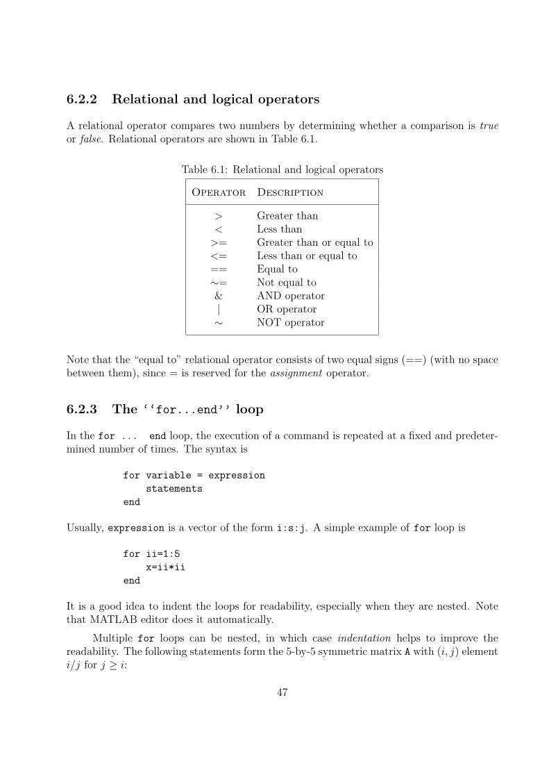
6.2.2 Relational and logical operators

A relational operator compares two numbers by determining whether a comparison is trueor false. Relational operators are shown in Table 6.1.

Table 6.1: Relational and logical operators

Operator Description

> Greater than< Less than

>= Greater than or equal to<= Less than or equal to== Equal to∼= Not equal to& AND operator| OR operator∼ NOT operator

Note that the “equal to” relational operator consists of two equal signs (==) (with no spacebetween them), since = is reserved for the assignment operator.

6.2.3 The ‘‘for...end’’ loop

In the for ... end loop, the execution of a command is repeated at a fixed and predeter-mined number of times. The syntax is

for variable = expression

statements

end

Usually, expression is a vector of the form i:s:j. A simple example of for loop is

for ii=1:5

x=ii*ii

end

It is a good idea to indent the loops for readability, especially when they are nested. Notethat MATLAB editor does it automatically.

Multiple for loops can be nested, in which case indentation helps to improve thereadability. The following statements form the 5-by-5 symmetric matrix A with (i, j) elementi/j for j ≥ i:

47

n = 5; A = eye(n);

for j=2:n

for i=1:j-1

A(i,j)=i/j;

A(j,i)=i/j;

end

end

6.2.4 The ‘‘while...end’’ loop

This loop is used when the number of passes is not specified. The looping continues until astated condition is satisfied. The while loop has the form:

while expression

statements

end

The statements are executed as long as expression is true.

x = 1

while x <= 10

x = 3*x

end

It is important to note that if the condition inside the looping is not well defined, the loopingwill continue indefinitely. If this happens, we can stop the execution by pressing Ctrl-C.

6.2.5 Other flow structures

• The break statement. A while loop can be terminated with the break statement,which passes control to the first statement after the corresponding end. The break

statement can also be used to exit a for loop.

• The continue statement can also be used to exit a for loop to pass immediately tothe next iteration of the loop, skipping the remaining statements in the loop.

• Other control statements include return, continue, switch, etc. For more detailabout these commands, consul MATLAB documentation.

48

6.2.6 Operator precedence

We can build expressions that use any combination of arithmetic, relational, and logicaloperators. Precedence rules determine the order in which MATLAB evaluates an expression.We have already seen this in the “Tutorial Lessons”.

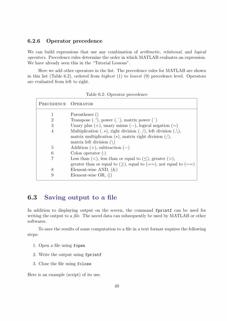
Here we add other operators in the list. The precedence rules for MATLAB are shownin this list (Table 6.2), ordered from highest (1) to lowest (9) precedence level. Operatorsare evaluated from left to right.

Table 6.2: Operator precedence

Precedence Operator

1 Parentheses ()2 Transpose (. ′), power (.ˆ), matrix power (ˆ)3 Unary plus (+), unary minus (−), logical negation (∼)4 Multiplication (. ∗), right division (. /), left division (.\),

matrix multiplication (∗), matrix right division (/),matrix left division (\)

5 Addition (+), subtraction (−)6 Colon operator (:)7 Less than (<), less than or equal to (≤), greater (>),

greater than or equal to (≥), equal to (==), not equal to (∼=)8 Element-wise AND, (&)9 Element-wise OR, (|)

6.3 Saving output to a file

In addition to displaying output on the screen, the command fprintf can be used forwriting the output to a file. The saved data can subsequently be used by MATLAB or othersoftwares.

To save the results of some computation to a file in a text format requires the followingsteps:

1. Open a file using fopen

2. Write the output using fprintf

3. Close the file using fclose

Here is an example (script) of its use.

49

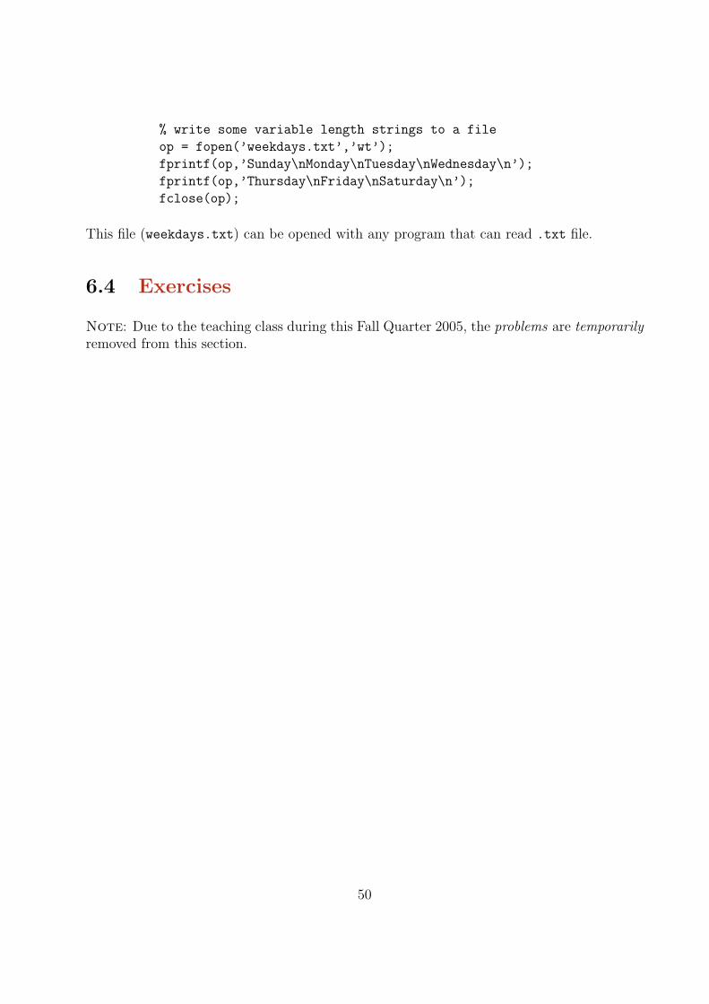
% write some variable length strings to a file

op = fopen(’weekdays.txt’,’wt’);

fprintf(op,’Sunday\nMonday\nTuesday\nWednesday\n’);

fprintf(op,’Thursday\nFriday\nSaturday\n’);

fclose(op);

This file (weekdays.txt) can be opened with any program that can read .txt file.

6.4 Exercises

Note: Due to the teaching class during this Fall Quarter 2005, the problems are temporarilyremoved from this section.

50

Chapter 7

Debugging M-files

7.1 Introduction

This section introduces general techniques for finding errors in M-files. Debugging is theprocess by which you isolate and fix errors in your program or code.

Debugging helps to correct two kind of errors:

• Syntax errors - For example omitting a parenthesis or misspelling a function name.

• Run-time errors - Run-time errors are usually apparent and difficult to track down.They produce unexpected results.

7.2 Debugging process

We can debug the M-files using the Editor/Debugger as well as using debugging functionsfrom the Command Window. The debugging process consists of

• Preparing for debugging

• Setting breakpoints

• Running an M-file with breakpoints

• Stepping through an M-file

• Examining values

• Correcting problems

• Ending debugging

51

7.2.1 Preparing for debugging

Here we use the Editor/Debugger for debugging. Do the following to prepare for debugging:

• Open the file

• Save changes

• Be sure the file you run and any files it calls are in the directories that are on thesearch path.

7.2.2 Setting breakpoints

Set breakpoints to pause execution of the function, so we can examine where the problemmight be. There are three basic types of breakpoints:

• A standard breakpoint, which stops at a specified line.

• A conditional breakpoint, which stops at a specified line and under specified conditions.

• An error breakpoint that stops when it produces the specified type of warning, error,NaN, or infinite value.

You cannot set breakpoints while MATLAB is busy, for example, running an M-file.

7.2.3 Running with breakpoints

After setting breakpoints, run the M-file from the Editor/Debugger or from the CommandWindow. Running the M-file results in the following:

• The prompt in the Command Window changes to

K>>

indicating that MATLAB is in debug mode.

• The program pauses at the first breakpoint. This means that line will be executedwhen you continue. The pause is indicated by the green arrow.

• In breakpoint, we can examine variable, step through programs, and run other callingfunctions.

52

7.2.4 Examining values

While the program is paused, we can view the value of any variable currently in theworkspace. Examine values when we want to see whether a line of code has producedthe expected result or not. If the result is as expected, step to the next line, and continuerunning. If the result is not as expected, then that line, or the previous line, contains anerror. When we run a program, the current workspace is shown in the Stack field. Use who

or whos to list the variables in the current workspace.

Viewing values as datatips

First, we position the cursor to the left of a variable on that line. Its current value appears.This is called a datatip, which is like a tooltip for data. If you have trouble getting thedatatip to appear, click in the line and then move the cursor next to the variable.

7.2.5 Correcting and ending debugging

While debugging, we can change the value of a variable to see if the new value producesexpected results. While the program is paused, assign a new value to the variable in the Com-mand Window, Workspace browser, or Array Editor. Then continue running and steppingthrough the program.

7.2.6 Ending debugging

After identifying a problem, end the debugging session. It is best to quit debug mode beforeediting an M-file. Otherwise, you can get unexpected results when you run the file. To enddebugging, select Exit Debug Mode from the Debug menu.

7.2.7 Correcting an M-file

To correct errors in an M-file,

• Quit debugging

• Do not make changes to an M-file while MATLAB is in debug mode

• Make changes to the M-file

• Save the M-file

• Clear breakpoints

53

• Run the M-file again to be sure it produces the expected results.

For details on debugging process, see MATLAB documentation.

54

Appendix A

Summary of commands

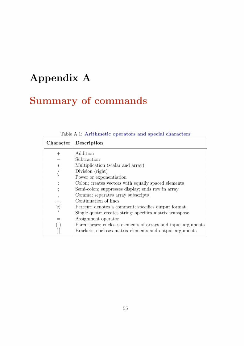
Table A.1: Arithmetic operators and special characters

Character Description

+ Addition− Subtraction∗ Multiplication (scalar and array)/ Division (right)ˆ Power or exponentiation: Colon; creates vectors with equally spaced elements; Semi-colon; suppresses display; ends row in array, Comma; separates array subscripts

. . . Continuation of lines% Percent; denotes a comment; specifies output format′ Single quote; creates string; specifies matrix transpose= Assignment operator( ) Parentheses; encloses elements of arrays and input arguments[ ] Brackets; encloses matrix elements and output arguments

55

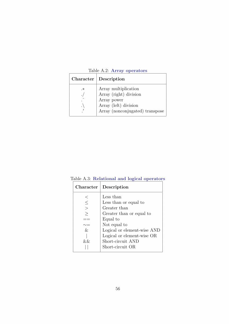
Table A.2: Array operators

Character Description

.∗ Array multiplication

./ Array (right) division

.ˆ Array power

.\ Array (left) division.′ Array (nonconjugated) transpose

Table A.3: Relational and logical operators

Character Description

< Less than≤ Less than or equal to> Greater than≥ Greater than or equal to

== Equal to∼= Not equal to& Logical or element-wise AND| Logical or element-wise OR

&& Short-circuit AND| | Short-circuit OR

56

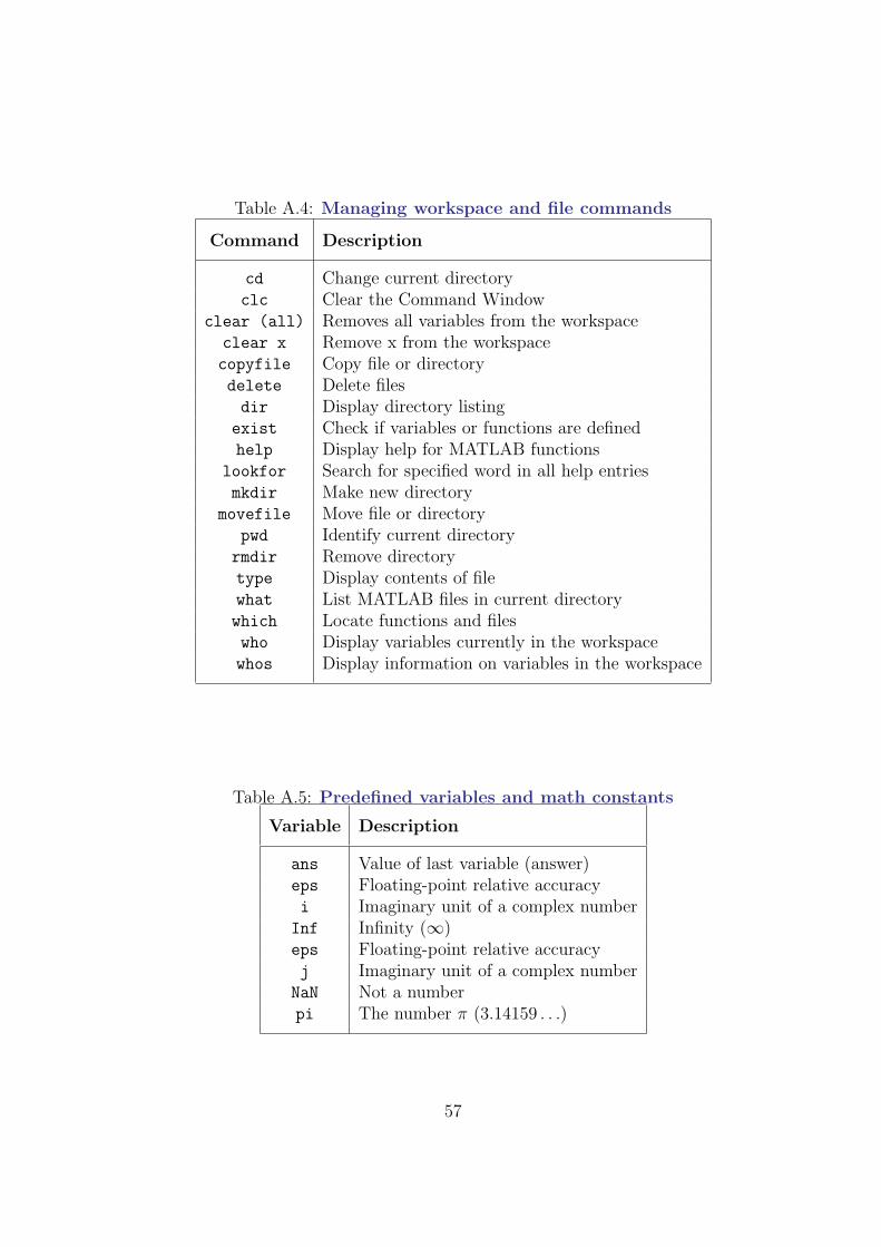
Table A.4: Managing workspace and file commands

Command Description

cd Change current directoryclc Clear the Command Window

clear (all) Removes all variables from the workspaceclear x Remove x from the workspacecopyfile Copy file or directorydelete Delete filesdir Display directory listing

exist Check if variables or functions are definedhelp Display help for MATLAB functions

lookfor Search for specified word in all help entriesmkdir Make new directory

movefile Move file or directorypwd Identify current directory

rmdir Remove directorytype Display contents of filewhat List MATLAB files in current directorywhich Locate functions and fileswho Display variables currently in the workspacewhos Display information on variables in the workspace

Table A.5: Predefined variables and math constants

Variable Description

ans Value of last variable (answer)eps Floating-point relative accuracyi Imaginary unit of a complex number

Inf Infinity (∞)eps Floating-point relative accuracyj Imaginary unit of a complex number

NaN Not a numberpi The number π (3.14159 . . .)

57

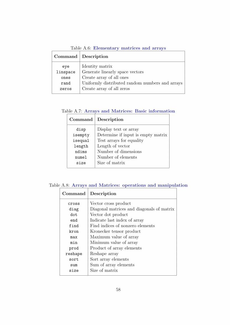
Table A.6: Elementary matrices and arrays

Command Description

eye Identity matrixlinspace Generate linearly space vectors

ones Create array of all onesrand Uniformly distributed random numbers and arrayszeros Create array of all zeros

Table A.7: Arrays and Matrices: Basic information

Command Description

disp Display text or arrayisempty Determine if input is empty matrixisequal Test arrays for equalitylength Length of vectorndims Number of dimensionsnumel Number of elementssize Size of matrix

Table A.8: Arrays and Matrices: operations and manipulation

Command Description

cross Vector cross productdiag Diagonal matrices and diagonals of matrixdot Vector dot productend Indicate last index of arrayfind Find indices of nonzero elementskron Kronecker tensor productmax Maximum value of arraymin Minimum value of arrayprod Product of array elements

reshape Reshape arraysort Sort array elementssum Sum of array elementssize Size of matrix

58

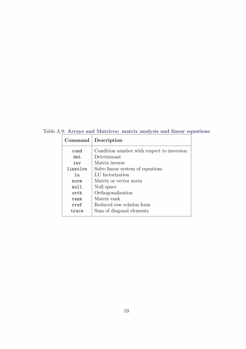
Table A.9: Arrays and Matrices: matrix analysis and linear equations

Command Description

cond Condition number with respect to inversiondet Determinantinv Matrix inverse

linsolve Solve linear system of equationslu LU factorization

norm Matrix or vector normnull Null spaceorth Orthogonalizationrank Matrix rankrref Reduced row echelon formtrace Sum of diagonal elements

59

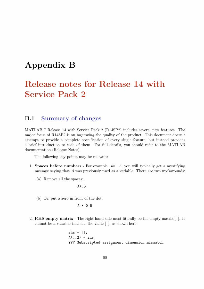
Appendix B

Release notes for Release 14 withService Pack 2

B.1 Summary of changes

MATLAB 7 Release 14 with Service Pack 2 (R14SP2) includes several new features. Themajor focus of R14SP2 is on improving the quality of the product. This document doesn’tattempt to provide a complete specification of every single feature, but instead providesa brief introduction to each of them. For full details, you should refer to the MATLABdocumentation (Release Notes).

The following key points may be relevant:

1. Spaces before numbers - For example: A* .5, you will typically get a mystifyingmessage saying that A was previously used as a variable. There are two workarounds:

(a) Remove all the spaces:

A*.5

(b) Or, put a zero in front of the dot:

A * 0.5

2. RHS empty matrix - The right-hand side must literally be the empty matrix [ ]. Itcannot be a variable that has the value [ ], as shown here:

rhs = [];

A(:,2) = rhs

??? Subscripted assignment dimension mismatch

60

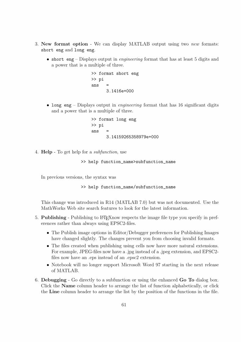
3. New format option - We can display MATLAB output using two new formats:short eng and long eng.

• short eng – Displays output in engineering format that has at least 5 digits anda power that is a multiple of three.

>> format short eng

>> pi

ans =

3.1416e+000

• long eng – Displays output in engineering format that has 16 significant digitsand a power that is a multiple of three.

>> format long eng

>> pi

ans =

3.14159265358979e+000

4. Help - To get help for a subfunction, use

>> help function_name>subfunction_name

In previous versions, the syntax was

>> help function_name/subfunction_name

This change was introduced in R14 (MATLAB 7.0) but was not documented. Use theMathWorks Web site search features to look for the latest information.

5. Publishing - Publishing to LATEXnow respects the image file type you specify in pref-erences rather than always using EPSC2-files.

• The Publish image options in Editor/Debugger preferences for Publishing Imageshave changed slightly. The changes prevent you from choosing invalid formats.

• The files created when publishing using cells now have more natural extensions.For example, JPEG-files now have a .jpg instead of a .jpeg extension, and EPSC2-files now have an .eps instead of an .epsc2 extension.

• Notebook will no longer support Microsoft Word 97 starting in the next releaseof MATLAB.

6. Debugging - Go directly to a subfunction or using the enhanced Go To dialog box.Click the Name column header to arrange the list of function alphabetically, or clickthe Line column header to arrange the list by the position of the functions in the file.

61

B.2 Other changes

1. There is a new command mlint, which will scan an M-file and show inefficiencies inthe code. For example, it will tell you if you’ve defined a variable you’ve never used, ifyou’ve failed to pre-allocate an array, etc. These are common mistakes in EA1 whichproduce runnable but inefficient code.

2. You can comment-out a block of code without putting % at the beginning of each line.The format is

%{

Stuff you want MATLAB to ignore...

%}

The delimiters %{ and %} must appear on lines by themselves, and it may not workwith the comments used in functions to interact with the help system (like the H1line).

3. There is a new function linsolve which will solve Ax = b but with the user’s choice ofalgorithm. This is in addition to left division x = A\b which uses a default algorithm.

4. The eps constant now takes an optional argument. eps(x) is the same as the oldeps*abs(x).

5. You can break an M-file up into named cells (blocks of code), each of which you canrun separately. This may be useful for testing/debugging code.

6. Functions now optionally end with the end keyword. This keyword is mandatory whenworking with nested functions.

B.3 Further details

1. You can dock and un-dock windows from the main window by clicking on an icon.Thus you can choose to have all Figures, M-files being edited, help browser, commandwindow, etc. All appear as panes in a single window.

2. Error messages in the command window resulting from running an M-file now includea clickable link to the offending line in the editor window containing the M-file.

3. You can customize figure interactively (labels, line styles, etc.) and then automaticallygenerate the code which reproduces the customized figure.

62

4. feval is no longer needed when working with function handles, but still works forbackward compatibility. For example, x=@sin; x(pi) will produce sin(pi) just likefeval(x,pi) does, but faster.

5. You can use function handles to create anonymous functions.

6. There is support for nested functions, namely, functions defined within the body ofanother function. This is in addition to sub-functions already available in version 6.5.

7. There is more support in arithmetic operations for numeric data types other thandouble, e.g. single, int8, int16, uint8, uint32, etc.

Finally, please visit our webpage for other details:

http://computing.mccormick.northwestern.edu/matlab/

63

Appendix C

Main characteristics of MATLAB

C.1 History

• Developed primarily by Cleve Moler in the 1970’s

• Derived from FORTRAN subroutines LINPACK and EISPACK, linear and eigenvaluesystems.

• Developed primarily as an interactive system to access LINPACK and EISPACK.

• Gained its popularity through word of mouth, because it was not officially distributed.

• Rewritten in C in the 1980’s with more functionality, which include plotting routines.

• The MathWorks Inc. was created (1984) to market and continue development ofMATLAB.

According to Cleve Moler, three other men played important roles in the origins of MATLAB:J. H. Wilkinson, George Forsythe, and John Todd. It is also interesting to mention theauthors of LINPACK: Jack Dongara, Pete Steward, Jim Bunch, and Cleve Moler. Sincethen another package emerged: LAPACK. LAPACK stands for Linear Algebra Package. Ithas been designed to supersede LINPACK and EISPACK.

C.2 Strengths

• MATLAB may behave as a calculator or as a programming language

• MATLAB combine nicely calculation and graphic plotting.

• MATLAB is relatively easy to learn

64

• MATLAB is interpreted (not compiled), errors are easy to fix

• MATLAB is optimized to be relatively fast when performing matrix operations

• MATLAB does have some object-oriented elements

C.3 Weaknesses

• MATLAB is not a general purpose programming language such as C, C++, or FOR-TRAN

• MATLAB is designed for scientific computing, and is not well suitable for other appli-cations

• MATLAB is an interpreted language, slower than a compiled language such as C++

• MATLAB commands are specific for MATLAB usage. Most of them do not have adirect equivalent with other programming language commands

C.4 Competition

• One of MATLAB’s competitors is Mathematica, the symbolic computation program.

• MATLAB is more convenient for numerical analysis and linear algebra. It is frequentlyused in engineering community.

• Mathematica has superior symbolic manipulation, making it popular among physicists.

• There are other competitors:

– Scilab

– GNU Octave

– Rlab

65

Bibliography

[1] The MathWorks Inc. MATLAB 7.0 (R14SP2). The MathWorks Inc., 2005.

[2] S. J. Chapman. MATLAB Programming for Engineers. Thomson, 2004.

[3] C. B. Moler. Numerical Computing with MATLAB. Siam, 2004.

[4] C. F. Van Loan. Introduction to Scientific Computing. Prentice Hall, 1997.

[5] D. J. Higham and N. J. Higham. MATLAB Guide. Siam, second edition edition, 2005.

[6] K. R. Coombes, B. R. Hunt, R. L. Lipsman, J. E. Osborn, and G. J. Stuck. DifferentialEquations with MATLAB. John Wiley and Sons, 2000.

[7] A. Gilat. MATLAB: An introduction with Applications. John Wiley and Sons, 2004.

[8] J. Cooper. A MATLAB Companion for Multivariable Calculus. Academic Press, 2001.

[9] J. C. Polking and D. Arnold. ODE using MATLAB. Prentice Hall, 2004.

[10] D. Kahaner, C. Moler, and S. Nash. Numerical Methods and Software. Prentice-Hall,1989.

[11] J. W. Demmel. Applied Numerical Linear Algebra. Siam, 1997.

[12] D. Houcque. Applications of MATLAB: Ordinary Differential Equations. Internalcommunication, Northwestern University, pages 1–12, 2005.

66