Introduction to Optimization!

Robert Stengel! Robotics and Intelligent Systems,

MAE 345, Princeton University, 2017

Optimization problems and criteriaCost functions

Static optimality conditionsExamples of static optimization

Copyright 2017 by Robert Stengel. All rights reserved. For educational use only.http://www.princeton.edu/~stengel/MAE345.html

1

Typical Optimization Problems

•! Minimize the probable error in an estimate of the dynamic state of a system

•! Maximize the probability of making a correct decision•! Minimize the time or energy required to achieve an

objective•! Minimize the regulation error in a controlled system

•!Estimation!•!Control!

2

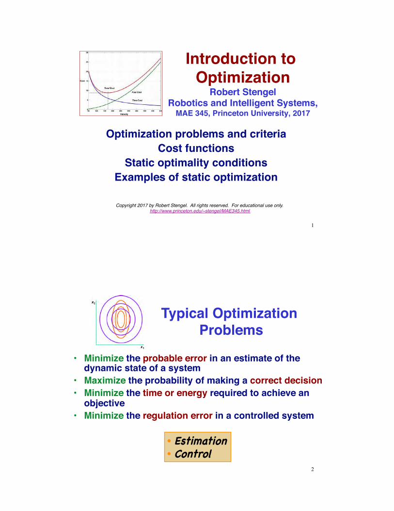
Optimization Implies Choice•! Choice of best strategy•! Choice of best design parameters•! Choice of best control history•! Choice of best estimate•! Optimization provided by selection

of the best control variable

3

Criteria for Optimization•! Names for criteria

–! Figure of merit–! Performance index–! Utility function–! Value function–! Fitness function–! Cost function, J

•! Optimal cost function = J*•! Optimal control = u*

•! Different criteria lead to different optimal solutions

•! Types of Optimality Criteria–! Absolute–! Regulatory–! Feasible

4

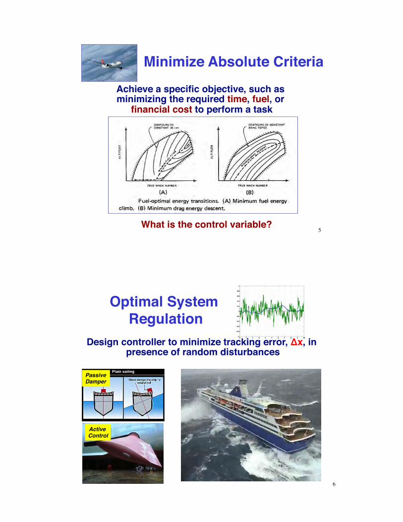
Minimize Absolute CriteriaAchieve a specific objective, such as minimizing the required time, fuel, or

financial cost to perform a task

What is the control variable?5

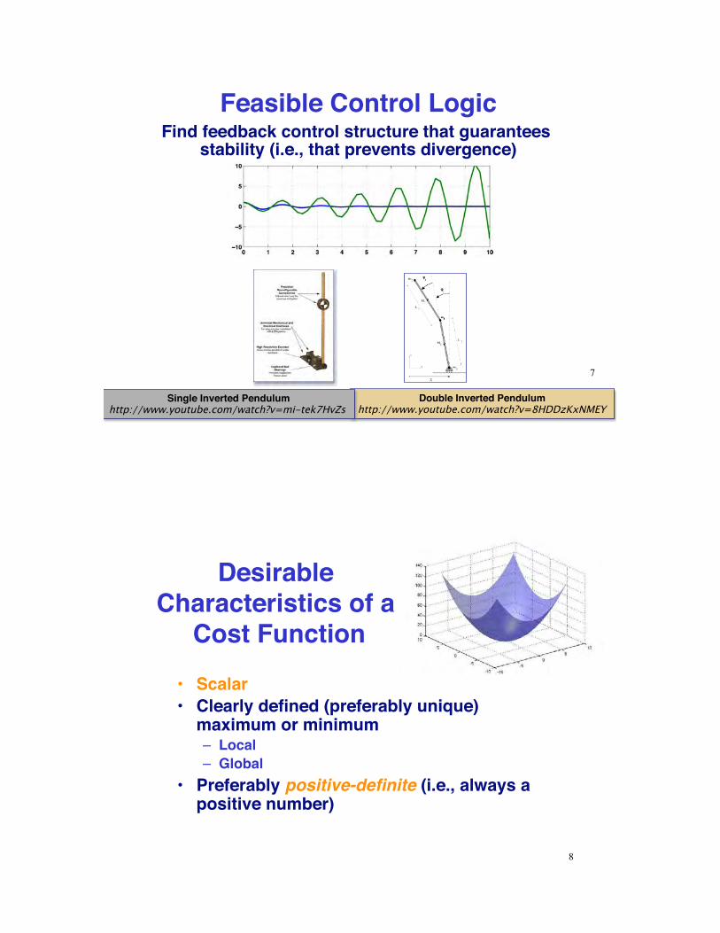
Optimal System Regulation

Design controller to minimize tracking error, "x, in presence of random disturbances

6

PassiveDamper

Active Control

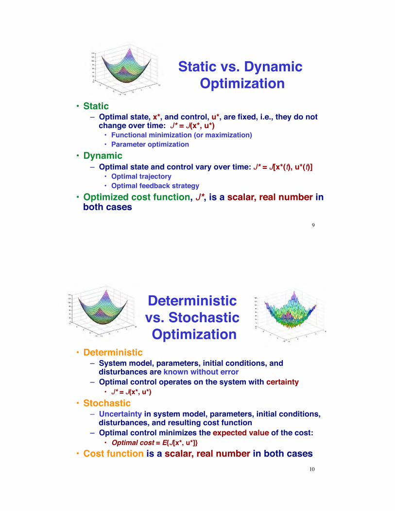
Feasible Control LogicFind feedback control structure that guarantees

stability (i.e., that prevents divergence)

Double Inverted Pendulumhttp://www.youtube.com/watch?v=8HDDzKxNMEY

Single Inverted Pendulumhttp://www.youtube.com/watch?v=mi-tek7HvZs

7

Desirable Characteristics of a

Cost Function•! Scalar•! Clearly defined (preferably unique)

maximum or minimum–! Local–! Global

•! Preferably positive-definite (i.e., always a positive number)

8

Static vs. Dynamic Optimization

•! Static–! Optimal state, x*, and control, u*, are fixed, i.e., they do not

change over time: J* = J(x*, u*)•! Functional minimization (or maximization)•! Parameter optimization

•! Dynamic–! Optimal state and control vary over time: J* = J[x*(t), u*(t)]

•! Optimal trajectory•! Optimal feedback strategy

•! Optimized cost function, J*, is a scalar, real number in both cases

9

Deterministic vs. Stochastic Optimization

•! Deterministic–! System model, parameters, initial conditions, and

disturbances are known without error–! Optimal control operates on the system with certainty

•! J* = J(x*, u*)•! Stochastic

–! Uncertainty in system model, parameters, initial conditions, disturbances, and resulting cost function

–! Optimal control minimizes the expected value of the cost: •! Optimal cost = E{J[x*, u*]}

•! Cost function is a scalar, real number in both cases10

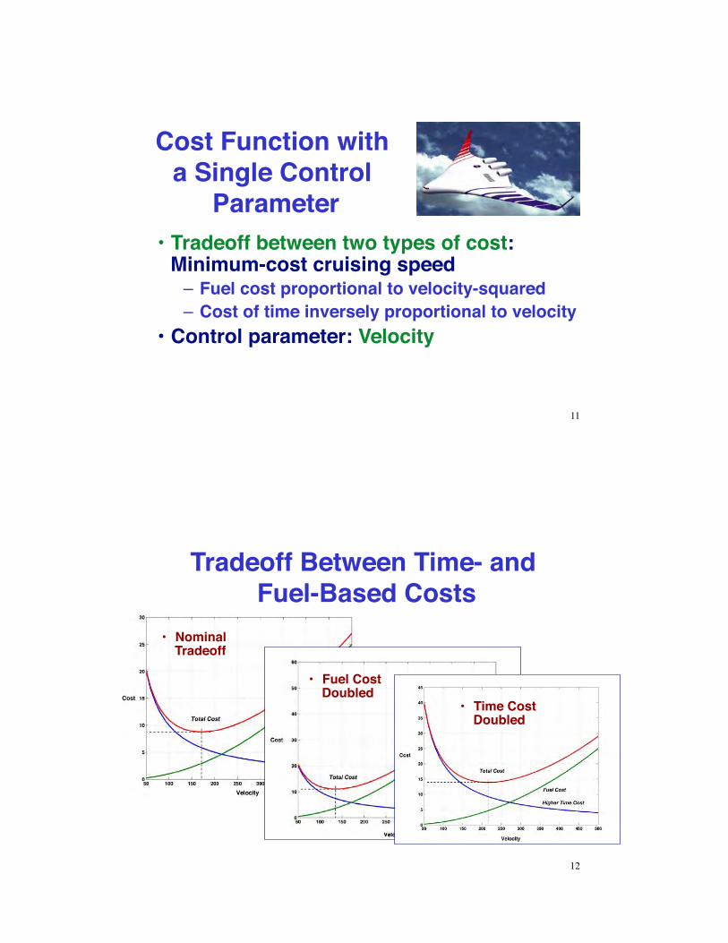
Cost Function with a Single Control

Parameter•!Tradeoff between two types of cost:

Minimum-cost cruising speed–! Fuel cost proportional to velocity-squared–! Cost of time inversely proportional to velocity

•!Control parameter: Velocity

11

Tradeoff Between Time- and Fuel-Based Costs

•! Nominal Tradeoff

•! Fuel Cost Doubled

•! Time Cost Doubled

12

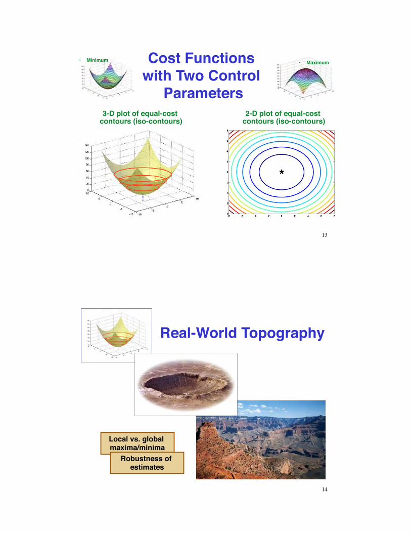
Cost Functions with Two Control

Parameters

•! Minimum •! Maximum

3-D plot of equal-cost contours (iso-contours)

2-D plot of equal-cost contours (iso-contours)

13

Real-World Topography

Local vs. global maxima/minima

Robustness of estimates

14

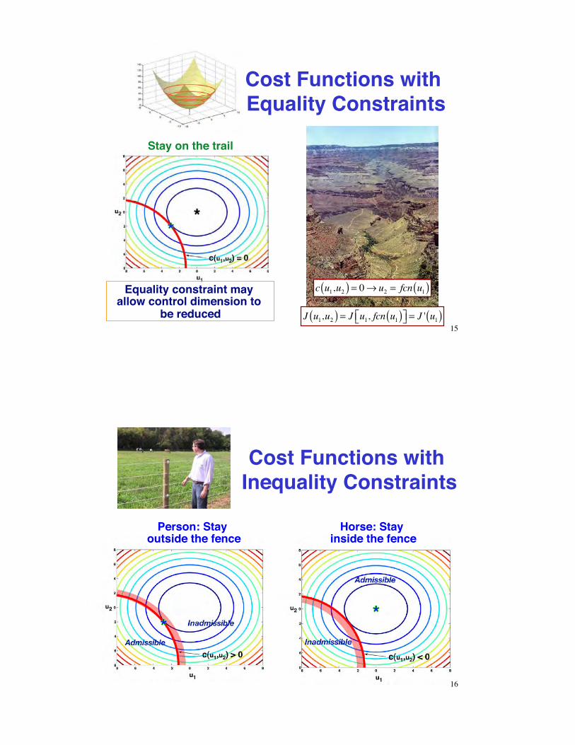
Stay on the trail

Equality constraint may allow control dimension to

be reduced

c u1,u2( ) = 0! u2 = fcn u1( )

15

Cost Functions with Equality Constraints

J u1,u2( ) = J u1, fcn u1( )!" #$ = J ' u1( )

Cost Functions with Inequality Constraints

Person: Stay outside the fence

Horse: Stay inside the fence

16

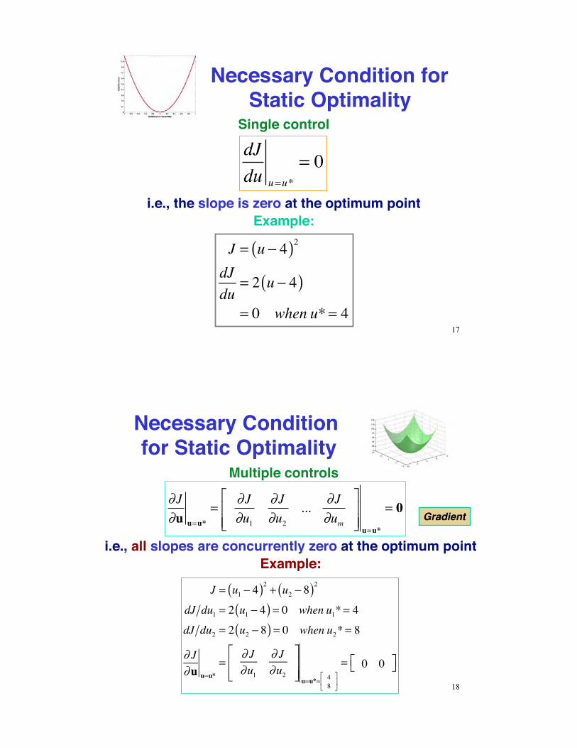
Necessary Condition for Static Optimality

Single control

dJdu u=u*

= 0

i.e., the slope is zero at the optimum pointExample:

J = u ! 4( )2

dJdu

= 2 u ! 4( )= 0 when u*= 4

17

Necessary Condition for Static Optimality

Multiple controls

i.e., all slopes are concurrently zero at the optimum pointExample:

!J!u u=u*

=!J!u1

!J!u2

... !J!um

"

#$$

%

&''u=u*

= 0

J = u1 ! 4( )2 + u2 ! 8( )2

dJ du1 = 2 u1 ! 4( ) = 0 when u1*= 4

dJ du2 = 2 u2 ! 8( ) = 0 when u2*= 8

" J"u u=u*

=" J"u1

" J"u2

#

$%%

&

'((u=u*= 4

8#

$%

&

'(

= 0 0#$ &'

Gradient

18

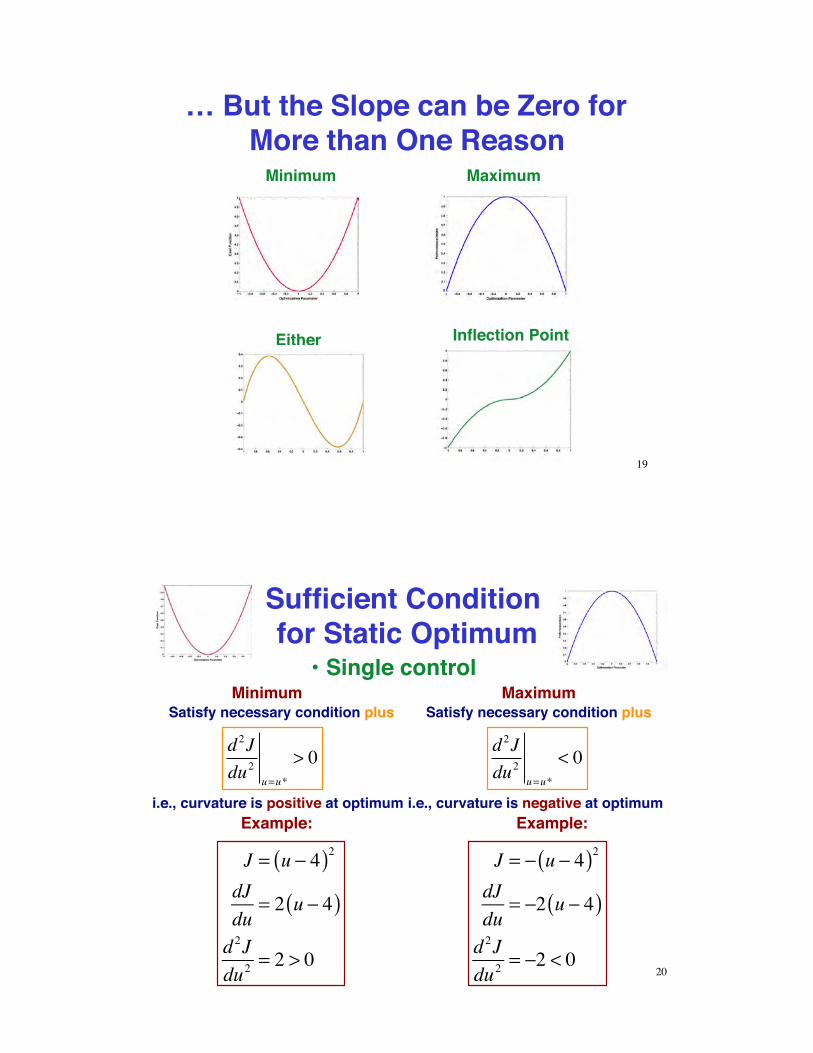
… But the Slope can be Zero for More than One Reason

Minimum

Either Inflection Point

Maximum

19

Sufficient Condition for Static Optimum

•!Single control

d 2Jdu2 u=u*

> 0

i.e., curvature is positive at optimumExample:

J = u ! 4( )2

dJdu

= 2 u ! 4( )d 2Jdu2

= 2 > 0

MinimumSatisfy necessary condition plus

d 2Jdu2 u=u*

< 0

i.e., curvature is negative at optimum Example:

J = ! u ! 4( )2

dJdu

= !2 u ! 4( )d 2Jdu2

= !2 < 0

MaximumSatisfy necessary condition plus

20

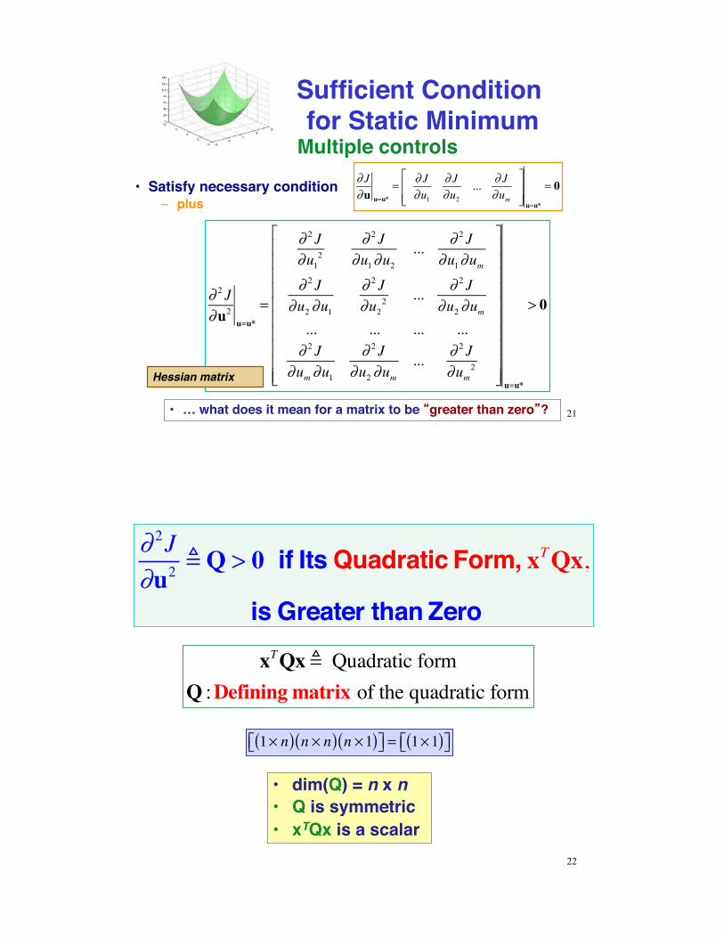
Sufficient Condition for Static Minimum

! 2 J!u2 u=u*

=

! 2 J!u1

2! 2 J

!u1!u2... ! 2 J

!u1!um! 2 J

!u2 !u1! 2 J!u2

2 ... ! 2 J!u2 !um

... ... ... ...! 2 J

!um !u1! 2 J

!u2 !um... ! 2 J

!um2

"

#

$$$$$$$$$$

%

&

''''''''''u=u*

> 0

•! Satisfy necessary condition–! plus

Hessian matrix

•! … what does it mean for a matrix to be greater than zero ?

! J!u u=u*

= ! J!u1

! J!u2

... ! J!um

"

#$$

%

&''u=u*

= 0

Multiple controls

21

! 2J!u2 ! Q > 0 if Its Quadratic Form, xTQx,

is Greater than Zero

xTQx ! Quadratic formQ :Defining matrix of the quadratic form

1! n( ) n ! n( ) n !1( )"# $% = 1!1( )"# $%

•! dim(Q) = n x n•! Q is symmetric•! xTQx is a scalar

22

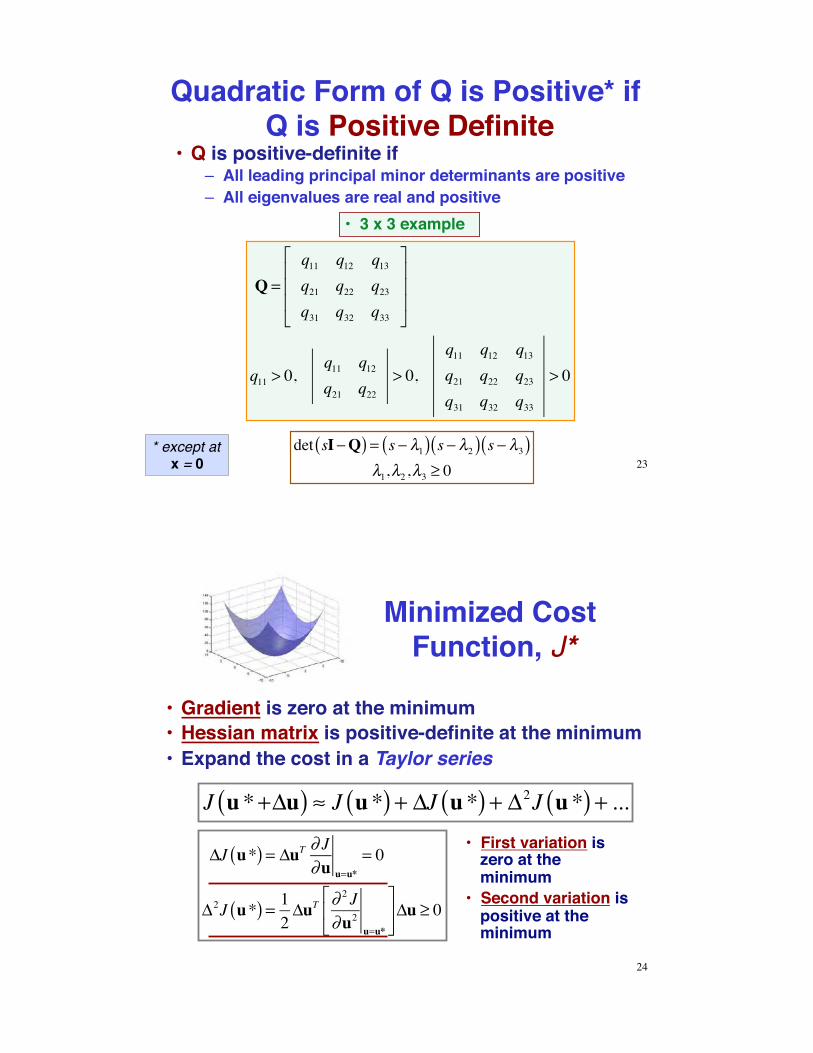
Q =q11 q12 q13q21 q22 q23q31 q32 q33

!

"

###

$

%

&&&

q11 > 0,q11 q12q21 q22

> 0,q11 q12 q13q21 q22 q23q31 q32 q33

> 0

•! Q is positive-definite if–! All leading principal minor determinants are positive–! All eigenvalues are real and positive

•! 3 x 3 example

det sI!Q( ) = s ! "1( ) s ! "2( ) s ! "3( )"1,"2,"3 # 0

Quadratic Form of Q is Positive* if Q is Positive Definite

* except at x = 0 23

!J u*( ) = !uT " J"u u=u*

= 0

!2J u*( ) = 12!uT " 2 J

"u2 u=u*

#

$%

&

'(!u ) 0

Minimized Cost Function, J*

•! First variation is zero at the minimum

•! Second variation is positive at the minimum

J u *+!u( ) " J u *( ) + !J u *( ) + !2J u *( ) + ...

•! Gradient is zero at the minimum•! Hessian matrix is positive-definite at the minimum•! Expand the cost in a Taylor series

24

•! Prior example

!J!u u=u*

=!J!u1

!J!u2

... !J!um

"

#$$

%

&''u=u*

= 0

! 2J!u2 u=u*

=

! 2J!u1

2

! 2J!u1!u2

... ! 2J!u1!um

! 2J!u2!u1

! 2J!u2

2 ... ! 2J!u2!um

... ... ... ...! 2J

!um!u1

! 2J!u2!um

... ! 2J!um

2

"

#

$$$$$$$$$$

%

&

''''''''''u=u*

>< 0

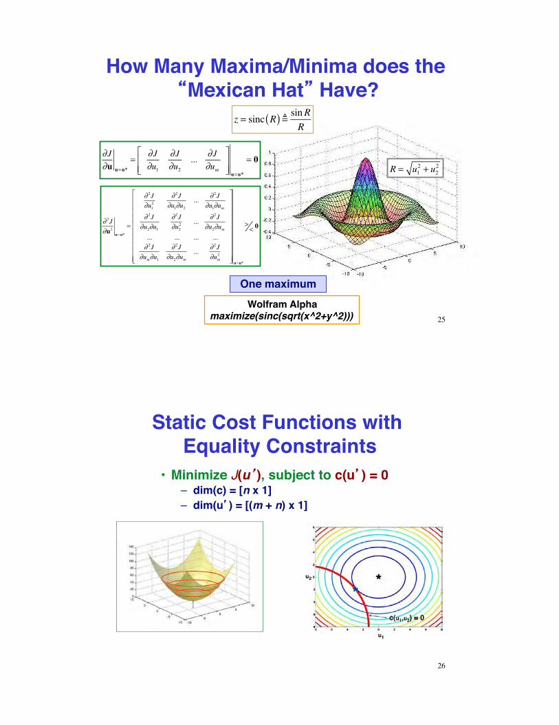
One maximum

R = u12 + u2

2

How Many Maxima/Minima does the Mexican Hat Have?

25

Wolfram Alphamaximize(sinc(sqrt(x^2+y^2)))

z = sinc R( ) ! sinR

R

Static Cost Functions with Equality Constraints

•! Minimize J(u ), subject to c(u ) = 0–! dim(c) = [n x 1]–! dim(u ) = [(m + n) x 1]

26

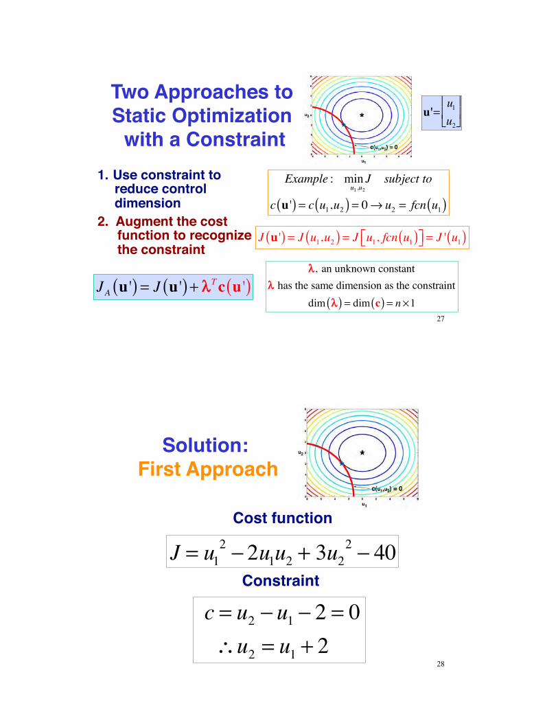
1.# Use constraint to reduce control dimension

2.# Augment the cost function to recognize the constraint

JA u '( ) = J u '( ) + !!Tc u '( )

Example : min Ju1,u2

subject to

c u '( ) = c u1,u2( ) = 0! u2 = fcn u1( )

u'=u1u2

!

" #

$

% &

Two Approaches to Static Optimization

with a Constraint

!!, an unknown constant!! has the same dimension as the constraint

dim !!( ) = dim c( ) = n "127

J u '( ) = J u1,u2( ) = J u1, fcn u1( )!" #$ = J ' u1( )

Solution: First Approach

Cost function

Constraint

J = u12 ! 2u1u2 + 3u2

2 ! 40

c = u2 ! u1 ! 2 = 0"u2 = u1 + 2

28

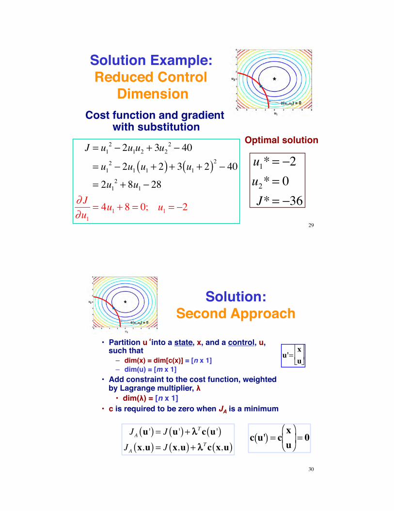
Solution Example: Reduced Control

Dimension

J = u12 ! 2u1u2 + 3u2

2 ! 40

= u12 ! 2u1 u1 + 2( ) + 3 u1 + 2( )2 ! 40

= 2u12 + 8u1 ! 28

" J"u1

= 4u1 + 8 = 0; u1 = !2

Cost function and gradient with substitution

Optimal solution

u1*= !2u2*= 0J*= !36

29

Solution:Second Approach

•! Partition u into a state, x, and a control, u, such that–! dim(x) = dim[c(x)] = [n x 1]–! dim(u) = [m x 1]

•! Add constraint to the cost function, weighted by Lagrange multiplier, $ •! dim($) = [n x 1]

•! c is required to be zero when JA is a minimum

u'=xu!

" # $

% &

c u'( ) = cxu!

" # $

% & = 0JA u '( ) = J u '( ) + !!Tc u '( )

JA x,u( ) = J x,u( ) + !!Tc x,u( )

30

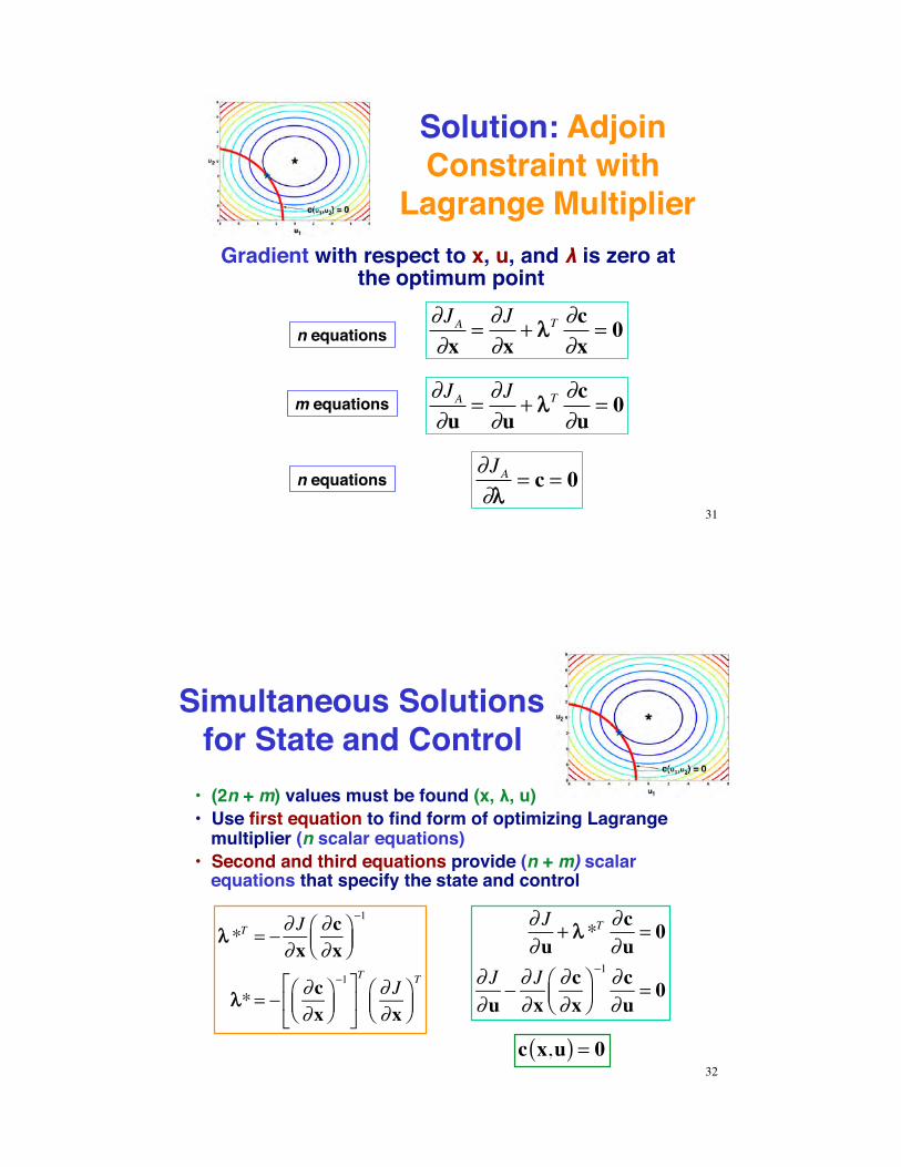
Solution: Adjoin Constraint with

Lagrange Multiplier

!JA!x

=!J!x

+ ""T !c!x

= 0

Gradient with respect to x, u, and ! is zero at the optimum point

!JA!u

=!J!u

+ ""T !c!u

= 0

!JA!""

= c = 031

n equations

m equations

n equations

Simultaneous Solutions for State and Control•! (2n + m) values must be found (x, $, u)•! Use first equation to find form of optimizing Lagrange

multiplier (n scalar equations)•! Second and third equations provide (n + m) scalar

equations that specify the state and control

!! *T = " # J#x

#c#x

$%&

'()"1

!!*= " #c#x

$%&

'()"1*

+,

-

./

T# J#x

$%&

'()T

! J!u

+ "" *T !c!u

= 0

! J!u

# ! J!x

!c!x

$%&

'()#1 !c!u

= 0

c x,u( ) = 032

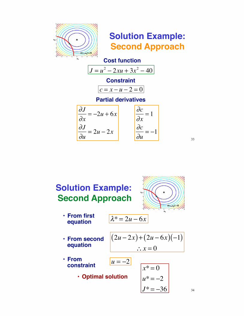
Solution Example: Second Approach

Cost function

ConstraintJ = u2 ! 2xu + 3x2 ! 40

c = x ! u ! 2 = 0

!J!x

= "2u + 6x

!J!u

= 2u " 2x

!c!x

= 1

!c!u

= "1

Partial derivatives

33

Solution Example: Second Approach

!* = 2u " 6x

2u ! 2x( ) + 2u ! 6x( ) !1( )" x = 0

x*= 0u*= !2J*= !36

•! Optimal solution

•! From first equation

•! From second equation

•! From constraint u = !2

34

Next Time:!Numerical Optimization!

35