Embed Size (px)
Citation preview

Introduction to Sensor Networks
Rabie A. Ramadan, PhDCairo University
http://rabieramadan.org
2
Deployment, Clustering , and and Routing in WSN
Deployment Constraints
Sensor characteristics
Monitored field characteristics
Monitored/probed object
3
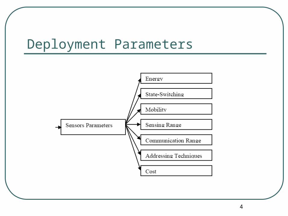
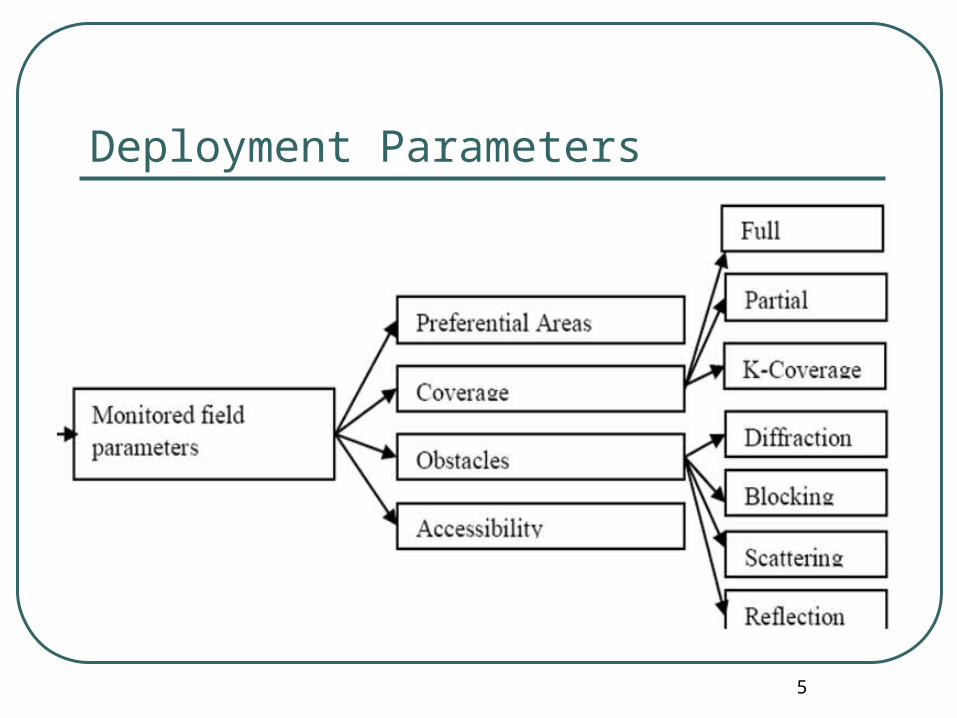
Deployment Parameters
4
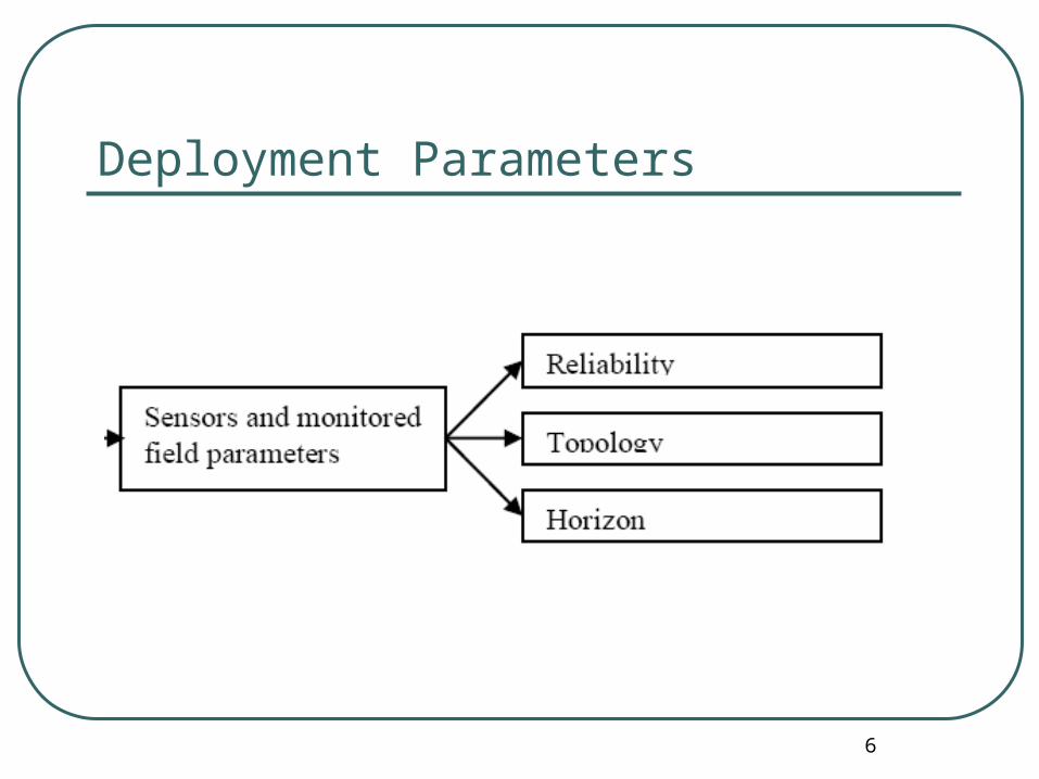
Deployment Parameters
5
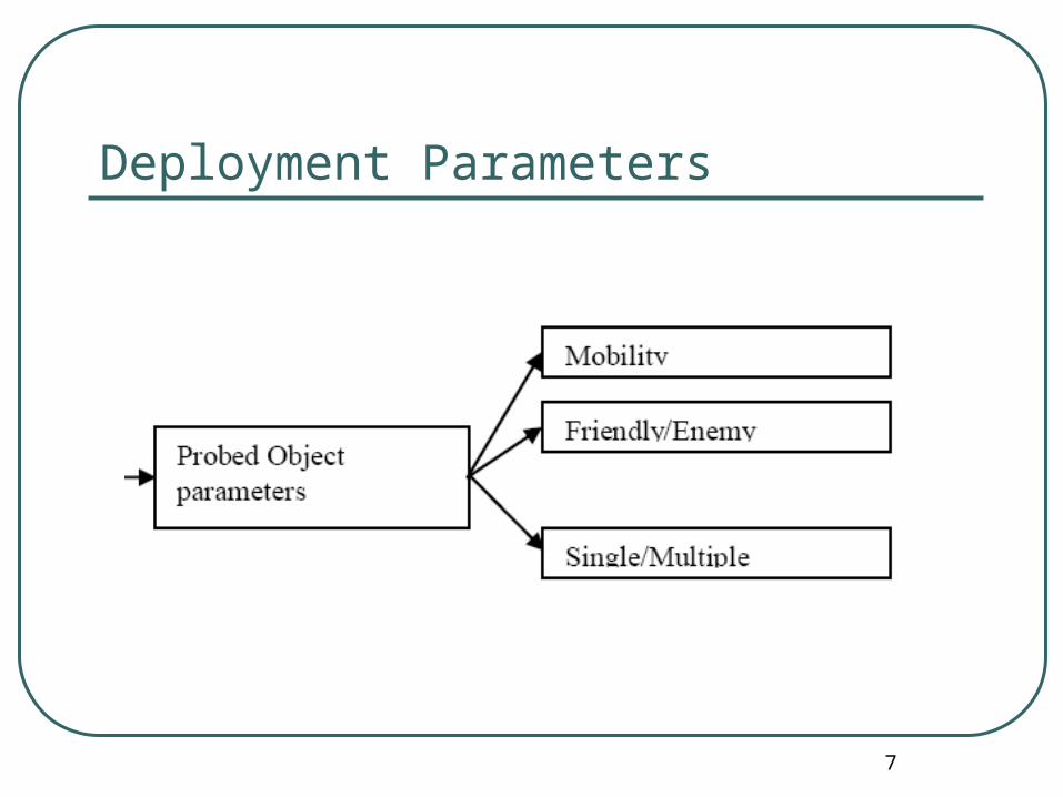
Deployment Parameters
6
Deployment Parameters
7
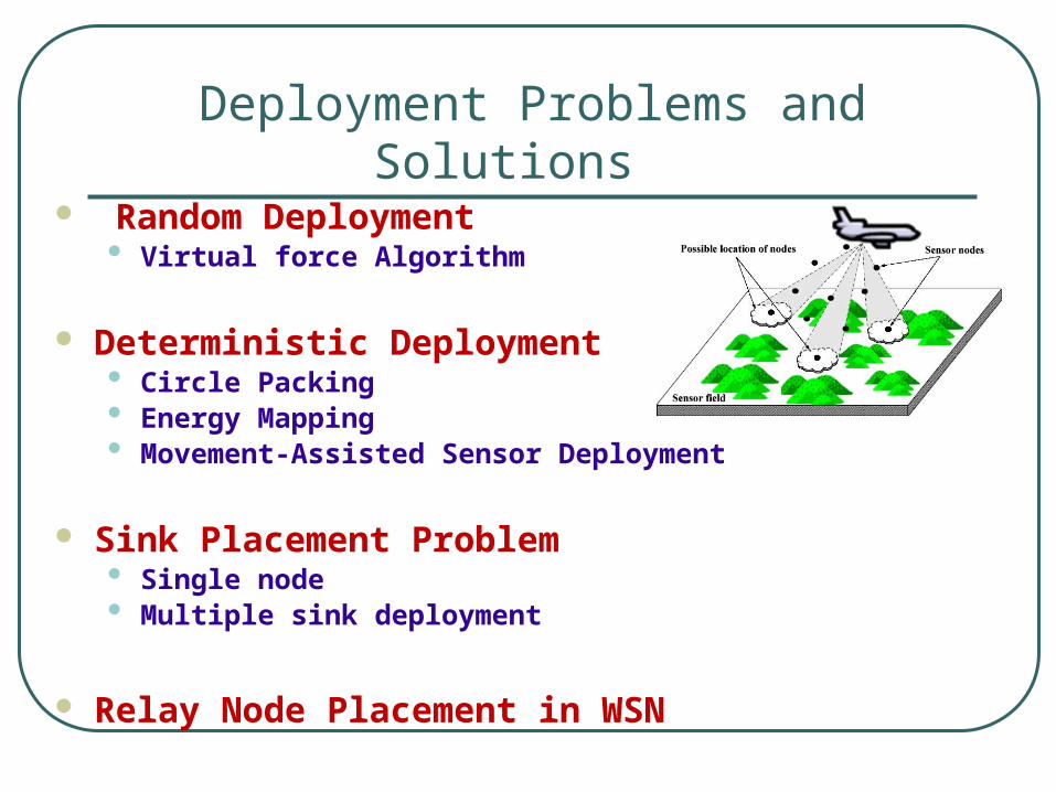
Deployment Problems and Solutions
Random Deployment • Virtual force Algorithm
Deterministic Deployment• Circle Packing • Energy Mapping • Movement-Assisted Sensor Deployment
Sink Placement Problem • Single node • Multiple sink deployment
Relay Node Placement in WSN
Random Deployment
Virtual Force Algorithm
9
Virtual Force Algorithm Sensors are initially deployed randomly Objective:
• To maximize the Coverage
Assume no prior knowledge about the monitored field
All nodes are mobile Energy and obstacles might present in the field
10
Virtual Force Algorithm (Cont.) Attractive and Repulsive forces
Sensors do not physically move
A sequence of virtual motion paths is determined for the randomly placed sensors.
Once the effective sensor positions are identified, a one-time movement is carried out to redeploy the sensors at these positions.
11
Virtual Force Algorithm (Semi Distributed.)
Assumptions:
• Clustered network
• All clustered heads are able to communicate with the sink node
• The cluster head is responsible for executing the VFA and managing the one-time movement of sensors to the desired locations.
12
Virtual Force Algorithm (Cont.) Each sensor behaves as a “Source of force” for all other
sensors.
This force can be either positive (Attractive) or negative (Repulsive).
The closeness and wide distance between two sensors are measured using a predefined threshold.
13
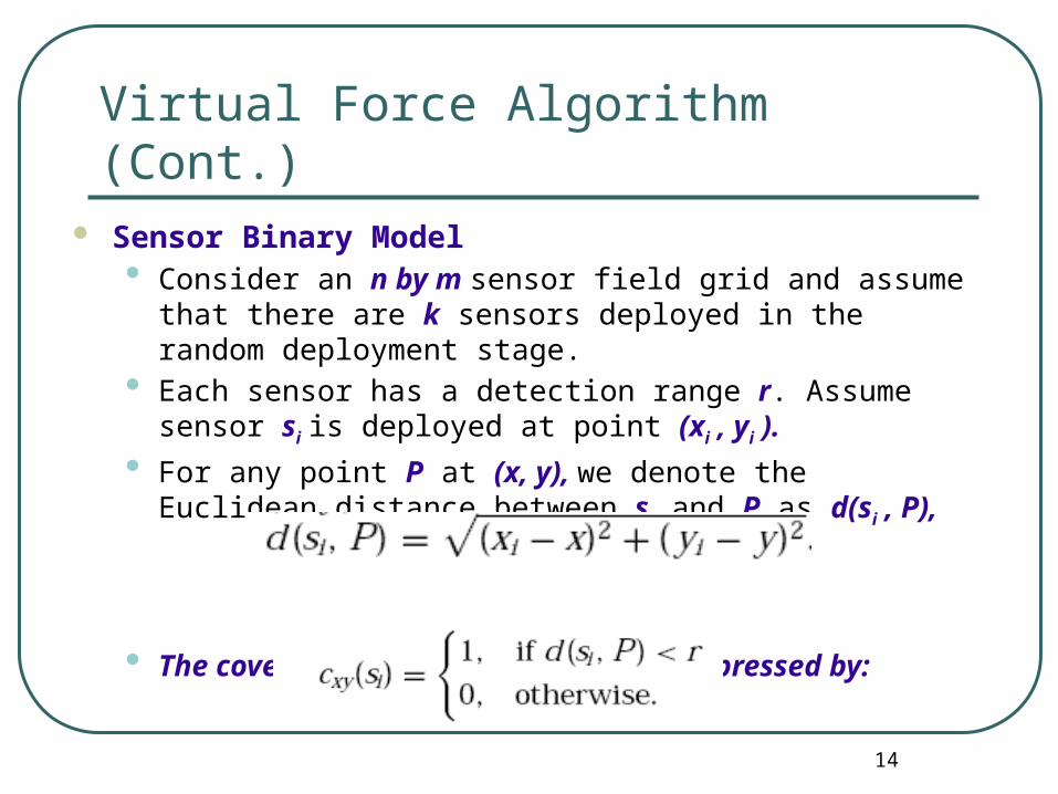
Virtual Force Algorithm (Cont.) Sensor Binary Model
• Consider an n by m sensor field grid and assume that there are k sensors deployed in the random deployment stage.
• Each sensor has a detection range r. Assume sensor si is deployed at point (xi , yi ).
• For any point P at (x, y), we denote the Euclidean distance between si and P as d(si , P),
• The coverage of a Grid Point P can be expressed by:
14
Virtual Force Algorithm (Cont.)
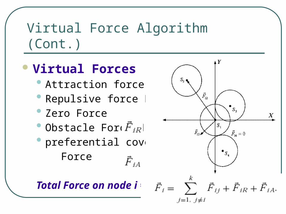
Virtual Forces• Attraction force F12• Repulsive force F13• Zero Force F14• Obstacle Force • preferential coverage
Force
Total Force on node i =
15
Virtual Force Algorithm (Cont.)
Energy Constraints • Using such forces , the cluster head runs the VFA • After stability occurs , Sensors are ordered to
move to the new positions
• Energy and Obstacles might be problems • Any sensor will not be able to move the required
distance , the moving order is discarded • Obstacles need an obstacle avoidance algorithm
16
Think…..
If some sensors are stationary, does this affect the virtual force algorithm?
17
SENSOR REPLACEMENT BASED ENERGY MAPPING
18
The problem
A set of sensors S is deployed in a monitored field F(A)for a period of time T.
The field is divided into a grid of cells A. Each cell is assigned a weight where represents the
importance of the cell i. The location of each sensor is assumed known; More than one sensor could be deployed in one cell. Sensors are assumed heterogeneous in terms of their
energy and mobility.
19
Assumptions
A sensor could be in different states; it could have its sensing off or on based on
the field monitoring requirements.• Sensing off, radio off – (sleep mode) • Sensing off, radio receiving – (Receiving mode) • Sensing off, radio transmitting – (Routing mode)• Sensing on, radio receiving – (Sensing and Receiving mode) • Sensing on, radio transmitting – (Sensing and Transmitting
mode)• Sensing on, radio off - (Sensing mode)
20
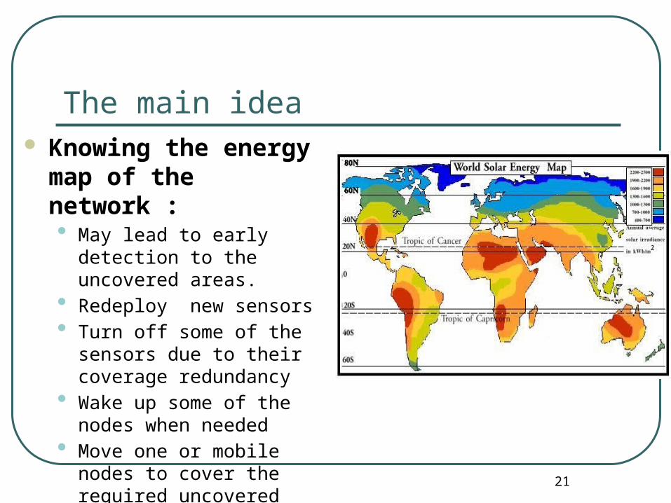
The main idea Knowing the energy map
of the network :• May lead to early detection to
the uncovered areas. • Redeploy new sensors• Turn off some of the sensors due
to their coverage redundancy • Wake up some of the nodes
when needed • Move one or mobile nodes to
cover the required uncovered spots
21
Redeployment based Energy map
Step 1: Energy dissipation rate prediction • Each sensor predicts its own energy rate based on its
history (e.g. Markov Chain ..)
Step 2: sensors send their initial energy and the location, predicted energy dissipation rate to the sink node through a cluster head. • Sensors update their energy dissipation rate based on a specific
threshold (if the new dissipation rate increased more than the given threshold , the node sends the new dissipation rate)
22
Redeployment based Energy map
Step 3: the sink node constructs the energy map based on the received dissipated energy rate from the sensors.
The sink may move one of the mobile sensors to the uncovered spot or wake up one of the sleeping sensors
23
Think …….
What are the disadvantages of energy mapping algorithm ?
24
Movement-Assisted Sensor
Deployment
25
The problem of sensor deployment
Given the target area, how to maximize the sensor coverage with less time, movement distance and message complexity
The importance of the problem• Distributed instead of centralized
26
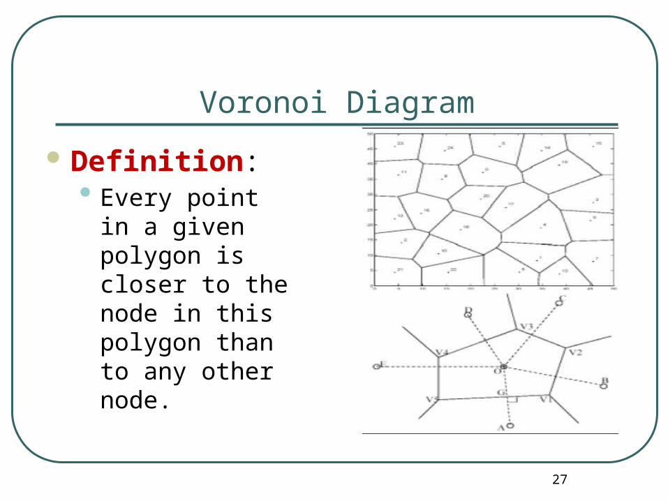
Voronoi Diagram
Definition:• Every point in a
given polygon is closer to the node in this polygon than to any other node.
27
Overview of the proposed algorithm
Sensors broadcast their locations and construct local Voronoi polygons
Find the coverage holes by examine Voronoi polygons
If holes exist, reduce coverage hole by moving• VOR : VORonoi-based
• Pull sensors to the sparsely covered area
28

Part of Assignment 2 Implement both Virtual Force algorithm and Voronoi based algorithm ? Report
your experience and algorithms efficiency?
Given a set of sensors with limited amount of energy. Some of these sensors are assumed mobile and others are assumed stationary. Assume similar sensing and communication ranges for all sensors. Sensors are allowed to move from one place to another iff they have enough energy to move to the required destination. In addition , the borders of the monitored area is assumed known in terms of 2D coordinates. Borders may be found in the monitored area. Advice a suitable deterministic deployment algorithm for efficient deployment to the sensors given that the deployed sensors have to be connected and important areas in the field are covered. In addition , your algorithm must guarantee the coverage of the monitored field for certain period of time.
You may look for an already given solution or come up with a convincing one .
29
30
Deterministic Deployment
Deployment Using Circle Packing
31
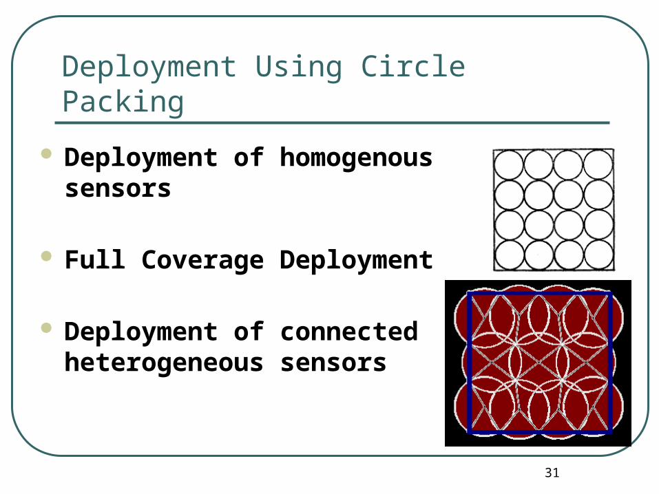
Deployment Using Circle Packing
Deployment of homogenous sensors
Full Coverage Deployment
Deployment of connected heterogeneous sensors
32
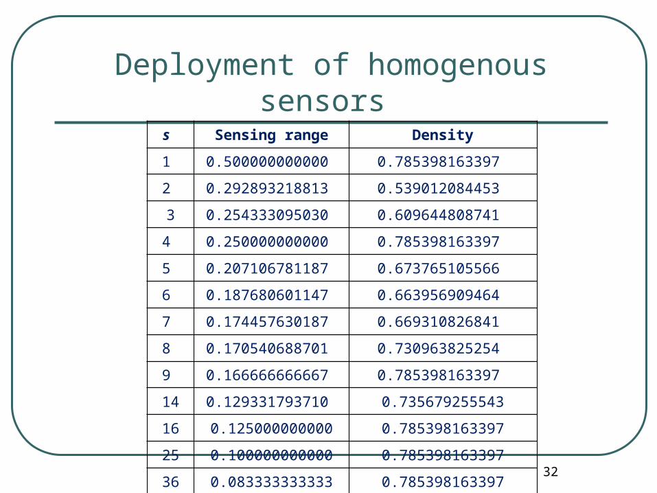
Deployment of homogenous sensors
s Sensing range Density
1 0.500000000000 0.785398163397
2 0.292893218813 0.539012084453
3 0.254333095030 0.609644808741
4 0.250000000000 0.785398163397
5 0.207106781187 0.673765105566
6 0.187680601147 0.663956909464
7 0.174457630187 0.669310826841
8 0.170540688701 0.730963825254
9 0.166666666667 0.785398163397
14 0.129331793710 0.735679255543
16 0.125000000000 0.785398163397
25 0.100000000000 0.785398163397
36 0.083333333333 0.785398163397
33
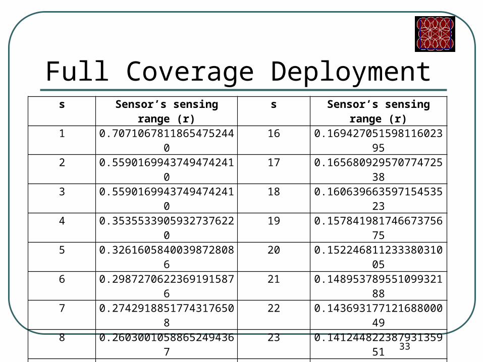
Full Coverage Deployment s Sensor’s sensing range (r) s Sensor’s sensing range (r)1 0.70710678118654752440 16 0.169427051598116023952 0.55901699437494742410 17 0.165680929570774725383 0.55901699437494742410 18 0.160639663597154535234 0.35355339059327376220 19 0.157841981746673756755 0.32616058400398728086 20 0.152246811233380310056 0.29872706223691915876 21 0.148953789551099321887 0.27429188517743176508 22 0.143693177121688000498 0.26030010588652494367 23 0.141244822387931359519 0.23063692781954790734 24 0.13830288328269767697
10 0.21823351279308384300 25 0.1335487065607704969311 0.21251601649318384587 26 0.1317648756148259646312 0.20227588920818008037 27 0.1286335345030996680713 0.19431237143171902878 28 0.1273175534656137214714 0.18551054726041864107 29 0.1255535079641135331715 0.17966175993333219846 30 0.12203686881944873607
34
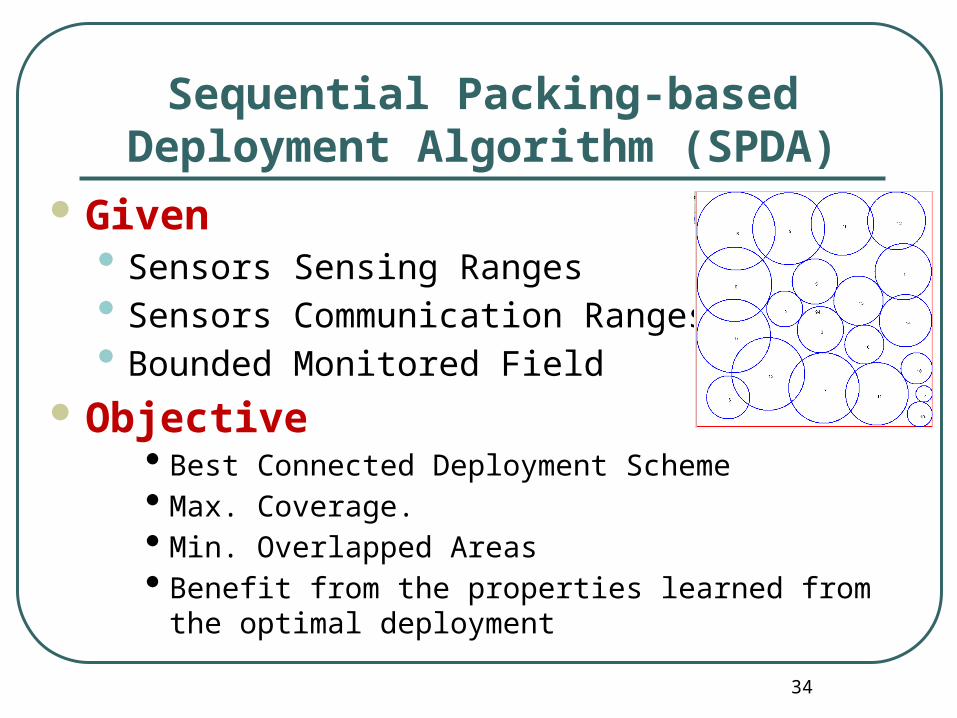
Sequential Packing-based Deployment Algorithm (SPDA)
Given • Sensors Sensing Ranges • Sensors Communication Ranges • Bounded Monitored Field
Objective • Best Connected Deployment Scheme • Max. Coverage.• Min. Overlapped Areas • Benefit from the properties learned from the optimal
deployment
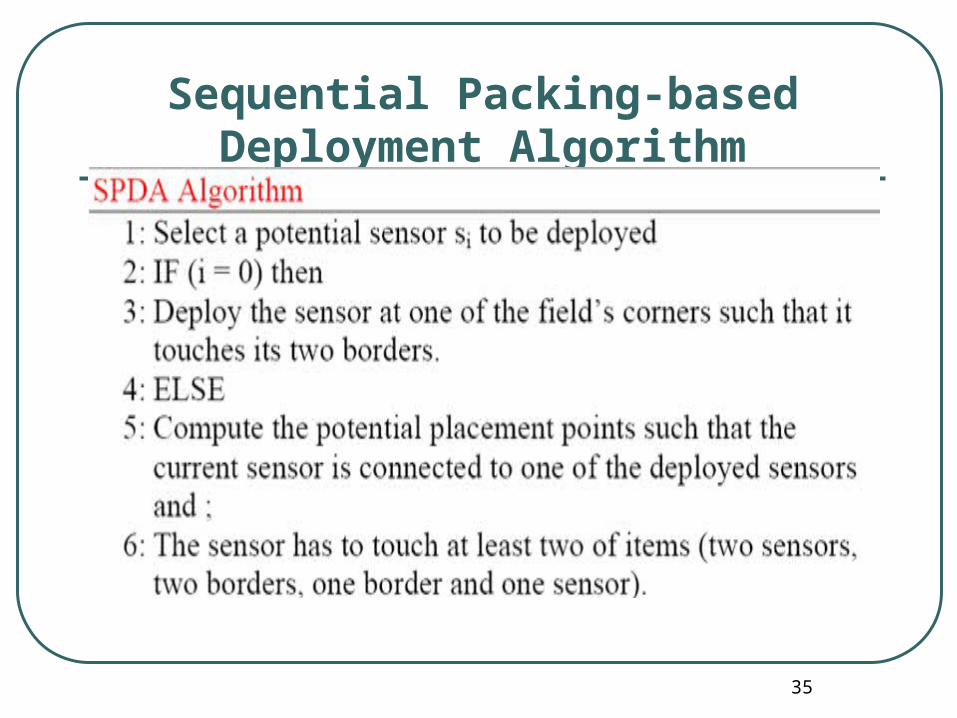
Sequential Packing-based Deployment Algorithm
35
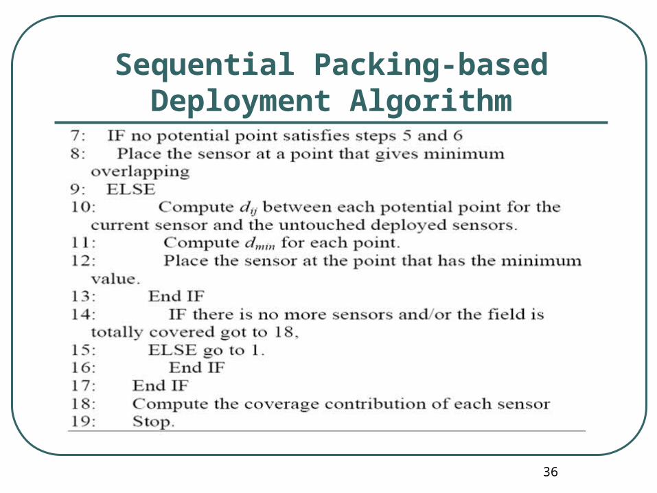
Sequential Packing-based Deployment Algorithm
36
37
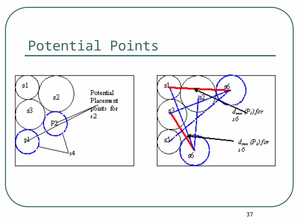
Potential Points
Think …..
38
How do you guarantee connectivity ?
39
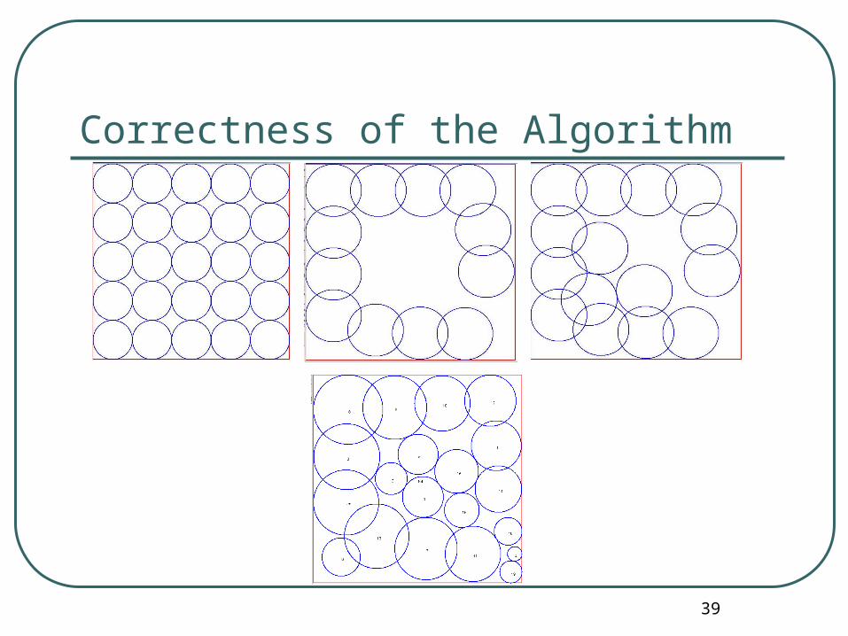
Correctness of the Algorithm
Sink Placement Problem
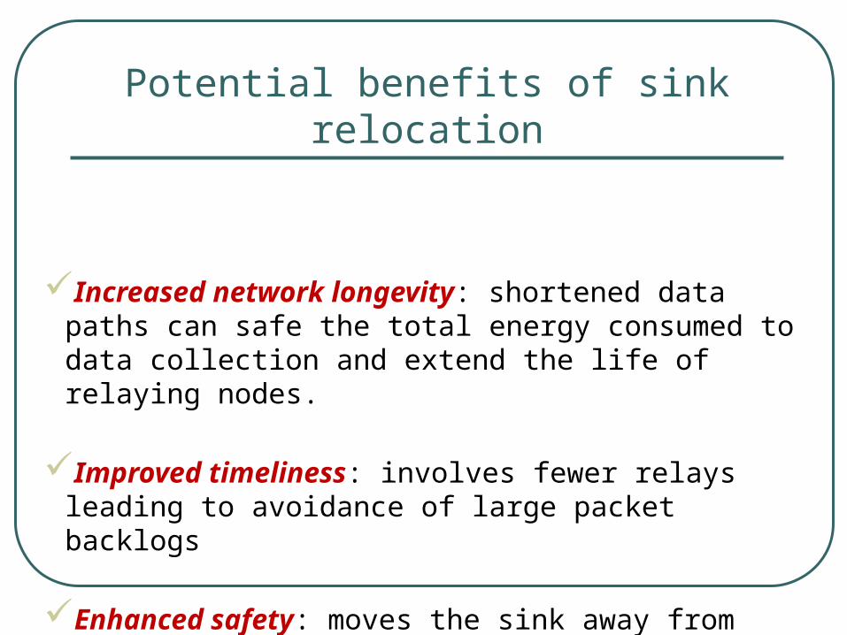
Potential benefits of sink relocation
Increased network longevity: shortened data paths can safe the
total energy consumed to data collection and extend the life of relaying nodes.
Improved timeliness: involves fewer relays leading to avoidance of large packet backlogs
Enhanced safety: moves the sink away from harmful events without damaging network performance
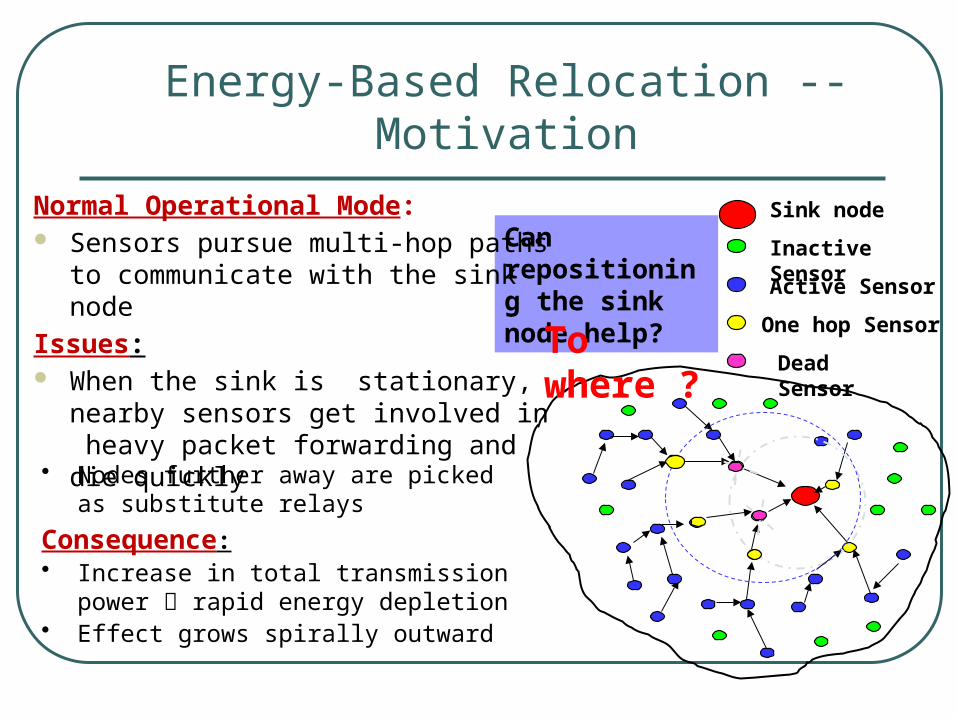
Energy-Based Relocation -- Motivation
Sink node
Inactive Sensor
Active Sensor
One hop Sensor
Dead Sensor
Can repositioning the sink node help?
Normal Operational Mode: Sensors pursue multi-hop paths to
communicate with the sink node
Issues: When the sink is stationary, nearby sensors
get involved in heavy packet forwarding and die quickly
• Nodes further away are picked as substitute relays
Consequence:• Increase in total transmission power rapid
energy depletion• Effect grows spirally outward
To where ?
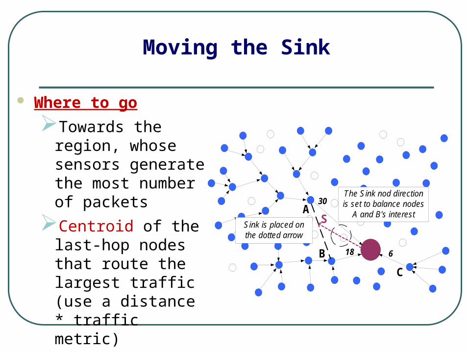
Moving the Sink
Where to go
Towards the region, whose sensors generate the most number of packets
Centroid of the last-hop nodes that route the largest traffic (use a distance * traffic metric)
B 18
30
6
A
The Sink nod directionis set to balance nodes
A and B's interestSink is placed onthe dotted arrow
C
S
Think….
What about putting the sink node initially in the center of all nodes? Does this will be the best position for the sink node?
44

Part of your assignment Device an algorithm for Multiple Sink Network Design
Problem in Large Scale Wireless Sensor Networks?
You may look at : • E. Ilker Oyman and Cem Ersoy,
Multiple Sink Network Design Problem in Large Scale Wireless Sensor Networks,, IEEE International Conference on Communications, 2004
Relay Node Placement in WSNClustering Algorithms
Clustering Facts Clustering plays a dominant role in delaying the first
node death, while aggregation plays a dominant role in delaying the last node death
In each cluster one node acts as a cluster head which is in charge of coordinating with other cluster heads
LEACH Algorithm The LEACH Network is made up of nodes, some of
which are called cluster-heads
• The job of the cluster-head is to collect data from their surrounding nodes and pass it on to the base station
• LEACH is dynamic because the job of cluster-head rotates LEACH is considered as clustering and routing
protocol
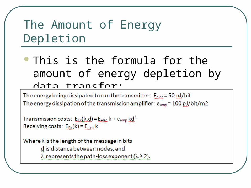
The Amount of Energy Depletion
This is the formula for the amount of energy depletion by data transfer:
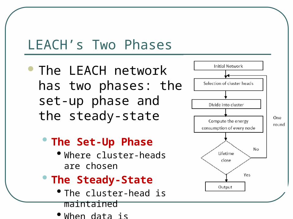
LEACH’s Two Phases
The LEACH network has two phases: the set-up phase and the steady-state
• The Set-Up Phase• Where cluster-heads are chosen
• The Steady-State• The cluster-head is maintained• When data is transmitted
between nodes
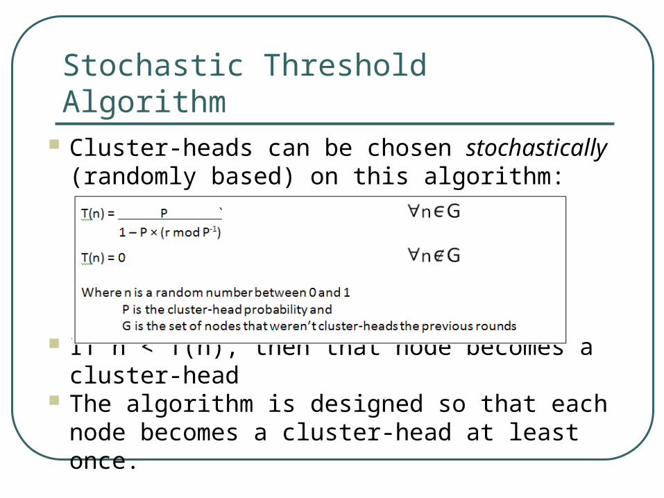
Stochastic Threshold Algorithm Cluster-heads can be chosen stochastically
(randomly based) on this algorithm:
If n < T(n), then that node becomes a cluster-head The algorithm is designed so that each node becomes
a cluster-head at least once.
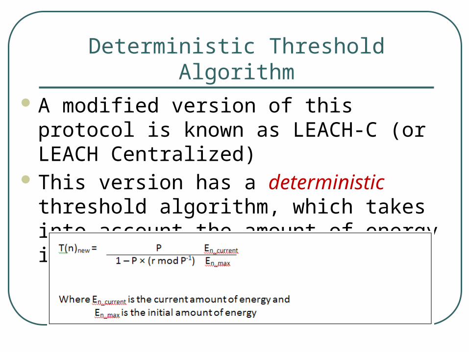
Deterministic Threshold Algorithm A modified version of this protocol is known as
LEACH-C (or LEACH Centralized) This version has a deterministic threshold
algorithm, which takes into account the amount of energy in the node…
Think more …..
How to modify LEACH to include more parameters such as node degree?
53
HEED: Hybrid Energy Efficient Distributed Clustering
HEED was designed to select different cluster heads in a field according to the amount of energy that is distributed in relation to a neighboring node.
Four primary goals: • prolonging network life-time by distributing energy
consumption• terminating the clustering process within a constant number of
iterations/steps• minimizing control overhead • producing well-distributed cluster heads and compact clusters.
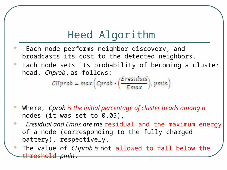
Heed Algorithm Each node performs neighbor discovery, and broadcasts its cost to the detected
neighbors. Each node sets its probability of becoming a cluster head, Chprob , as follows:
Where, Cprob is the initial percentage of cluster heads among n nodes (it was set to 0.05),
Eresidual and Emax are the residual and the maximum energy of a node (corresponding to the fully charged battery), respectively.
The value of CHprob is not allowed to fall below the threshold pmin .
Disadvantage (LEACH and HEED) – think….
Nodes’ score is computed based on node identifiers, and each node holds its message transmission until all its neighbors with lower IDs have done so.
Each node stops its protocol execution if it knows that every node in its neighborhood has transmitted.
It is assumed that the network topology does not change during the algorithm execution, and it is thus valid for each node to wait until it overhears every higher-scored neighbor transmitting.
56
Think…
How to solve Heed’s problems?
57
HEED Assignment Previous Algorithm is used with homogenous sensors (all have
the same characteristics ).
Device another clustering algorithm for heterogeneous WSN (nodes with different capabilities) .
You may have a look at the following paper
• Harneet Kour and Ajay K. Sharma, “Hybrid Energy Efficient Distributed Protocol for Heterogeneous Wireless Sensor Network, ” International Journal of Computer Applications (0975 – 8887) Volume 4 – No.6, July 2010
Mobility Resistant Clustering in Multi-Hop Wireless Networks --- Distributed Efficient Clustering Approach (DECA) ---
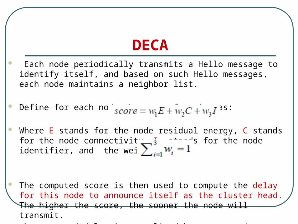
DECA Each node periodically transmits a Hello message to identify itself, and based
on such Hello messages, each node maintains a neighbor list.
Define for each node the score function as:
Where E stands for the node residual energy, C stands for the node connectivity, I stands for the node identifier, and the weights follow
The computed score is then used to compute the delay for this node to announce itself as the cluster head. The higher the score, the sooner the node will transmit.
The computed delay is normalized between 0 and a certain upper bound Dmax
Think…
How mobility can affect DECA algorithm?
61
Multimodal Limited Similarity Clustering (MFLC)
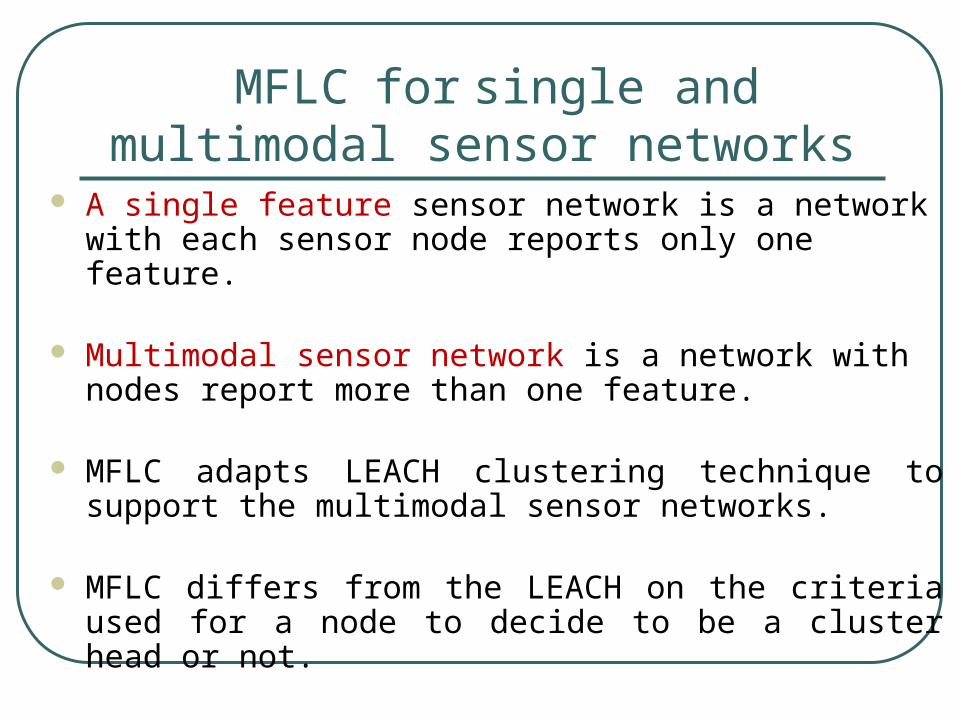
MFLC for single and multimodal sensor networks
A single feature sensor network is a network with each sensor node reports only one feature.
Multimodal sensor network is a network with nodes report more than one feature.
MFLC adapts LEACH clustering technique to support the multimodal sensor networks.
MFLC differs from the LEACH on the criteria used for a node to decide to be a cluster head or not.
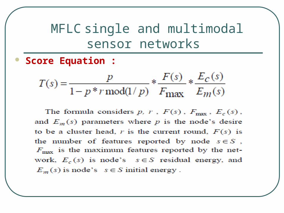
MFLC single and multimodal sensor networks
Score Equation :
Data Similarity Clustering Based Fuzzy Logic (DSBF)
DSBF
Phase One: Computing Node Degrees
Phase Two: Cluster Head Election
Phase Three: Data Reporting
Phase One: Computing Node Degrees
The node degree based similarity feature is computed
The node degree in this context means the number of similar sensors around Ss
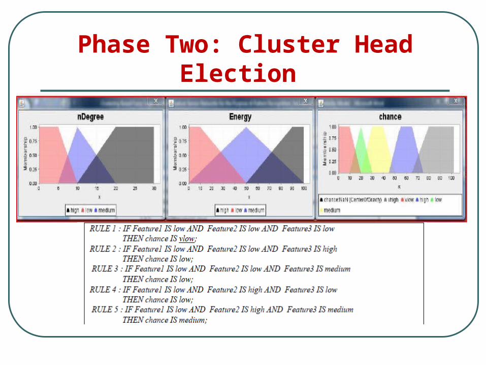
Phase Two: Cluster Head Election
Routing in WSN
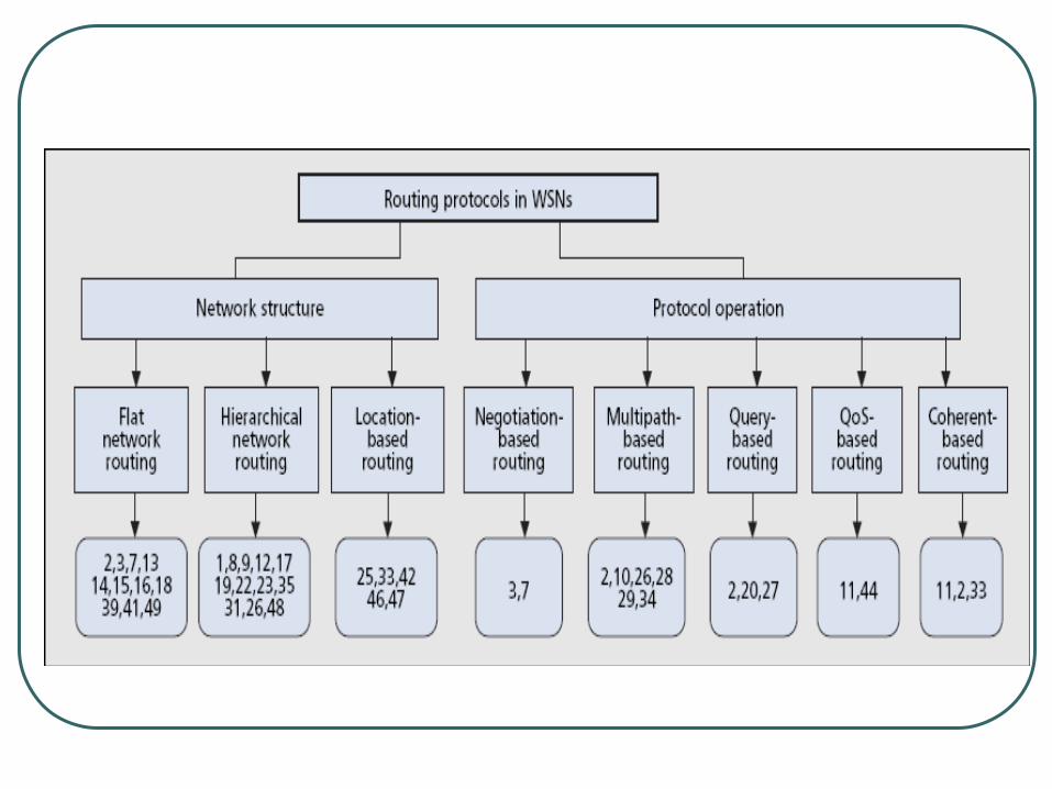
Flat Routing Each node plays the same role Data-centric routing
• Due to not feasible to assign a global id to each node• Save energy through data negotiation and elimination of redundant data
Protocols• Sensor Protocols for Information via Negotiation (SPIN)• Directed diffusion (DD)• Rumor routing• Minimum Cost Forwarding Algorithm (MCFA)• Gradient-based routing (GBR)• Information-driven sensor querying/Constrained anisotropic diffusion routing
(IDSQ/CADR)• COUGAR• ACQUIRE• Energy-Aware Routing• Routing protocols with random walks
Features• Negotiation
• to operate efficiently and to conserve energy• using a meta-data
• Resource adaptation• To extend the operating lifetime of the system• monitoring their own energy resources
SPIN Message• ADV – new data advertisement• REQ – request for ADV data• DATA – actual data message
• ADV, REQ messages contain only meta-data
Sensor protocols for information via negotiation (SPIN)
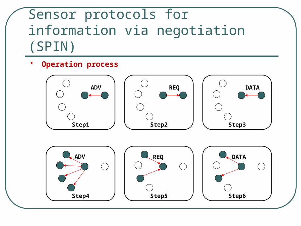
Sensor protocols for information via negotiation (SPIN)• Operation process
Step1
ADV
Step3
DATA
Step2
REQ
Step4
ADV
Step5
REQ
Step6
DATA
Sensor protocols for information via negotiation (SPIN)
Resource adaptive algorithm• When energy is plentiful
• Communicate using the 3-stage handshake protocol• When energy is approaching a low-energy threshold
• If a node receives ADV, it does not send out REQ• Energy is reserved to sensing the event
Advantage • Simplicity
• Each node performs little decision making when it receives new data
• Need not forwarding table• Robust to topology change
Drawback • Large overhead
• Data broadcasting
Think…. In SPIN
What about mobile nodes?
What about the multimodal Wireless nodes?
75
Directed Diffusion (DD) Feature
• Data-centric routing protocol• A path is established between sink node and source node• Localized interactions
• The propagation and aggregation procedures are all based on local information
Four elements• Interest
• A task description which is named by a list of attribute-value pairs that describe a task
• Gradient• Path direction, data transmission rate
• Data message• Reinforcement
• To select a single path from multiple paths
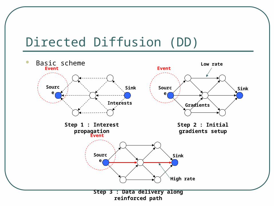
Directed Diffusion (DD) Basic scheme
SinkSource
Step 1 : Interest propagation
Interests
Event
SinkSource
Step 2 : Initial gradients setup
Gradients
EventLow rate
SinkSource
Step 3 : Data delivery along reinforced path
Event
High rate
Directed Diffusion (DD) Advantage
• Small delay• Always transmit the data through shortest path
• Robust to failed path
Drawback• Imbalance of node lifetime
• The energy of node on shortest path is drained faster than another• Time synchronization technique
• To implement data aggregation• Not easy to realize in a sensor network
• The overhead involved in recording information• Increasing the cost of a sensor node
Think…. In DD
What about mobile nodes?
What about the multimodal Wireless nodes?
79
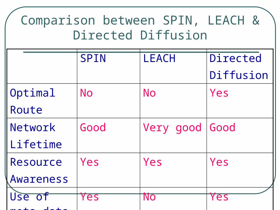
Comparison between SPIN, LEACH & Directed Diffusion
SPIN LEACH DirectedDiffusion
OptimalRoute
No No Yes
NetworkLifetime
Good Very good Good
ResourceAwareness
Yes Yes Yes
Use of meta-data
Yes No Yes
Feature • Combine query flooding and event flooding• Discovering arbitrary paths instead of the shortest path• Rumor routing is attractive only when
• The number of queries is larger than a threshold• The number of events is smaller than another threshold
Assumption• The network is composed of densely distributed nodes• Only short distance transmissions• Immobile nodes
Rumor Routing
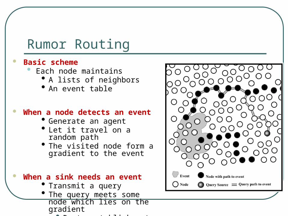
Rumor Routing Basic scheme
• Each node maintains• A lists of neighbors• An event table
When a node detects an event• Generate an agent• Let it travel on a random path• The visited node form a gradient to
the event
When a sink needs an event• Transmit a query • The query meets some node which
lies on the gradient• Route establishment
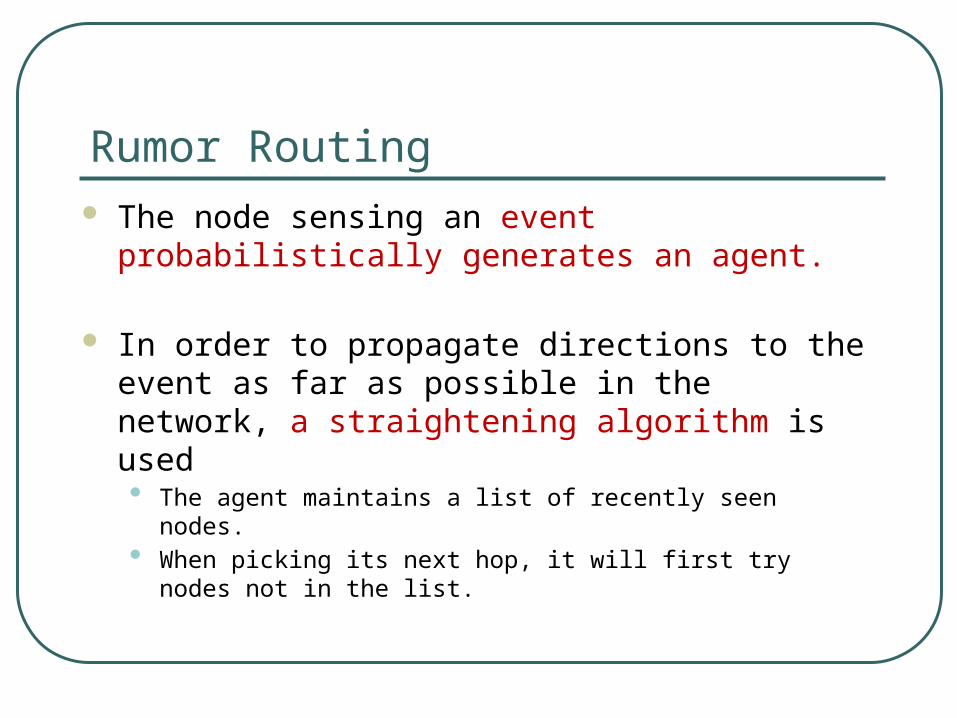
Rumor Routing The node sensing an event probabilistically generates an
agent.
In order to propagate directions to the event as far as possible in the network, a straightening algorithm is used• The agent maintains a list of recently seen nodes.• When picking its next hop, it will first try nodes not in the list.
Think…. In Rumor Routing
What about mobile nodes?
What about the multimodal Wireless nodes?
84

Minimum Cost Forwarding Algorithm (MCFA)
Objective • Establish the cost field• Transmit the data through the minimum-cost path
Feature• Optimality
• Minimum cost path criteria : hop count, energy consumption, delay etc.
• Simplicity• Need not to maintain forwarding table• Need not to know an ID for a neighbor node
Minimum Cost Forwarding Algorithm (MCFA)
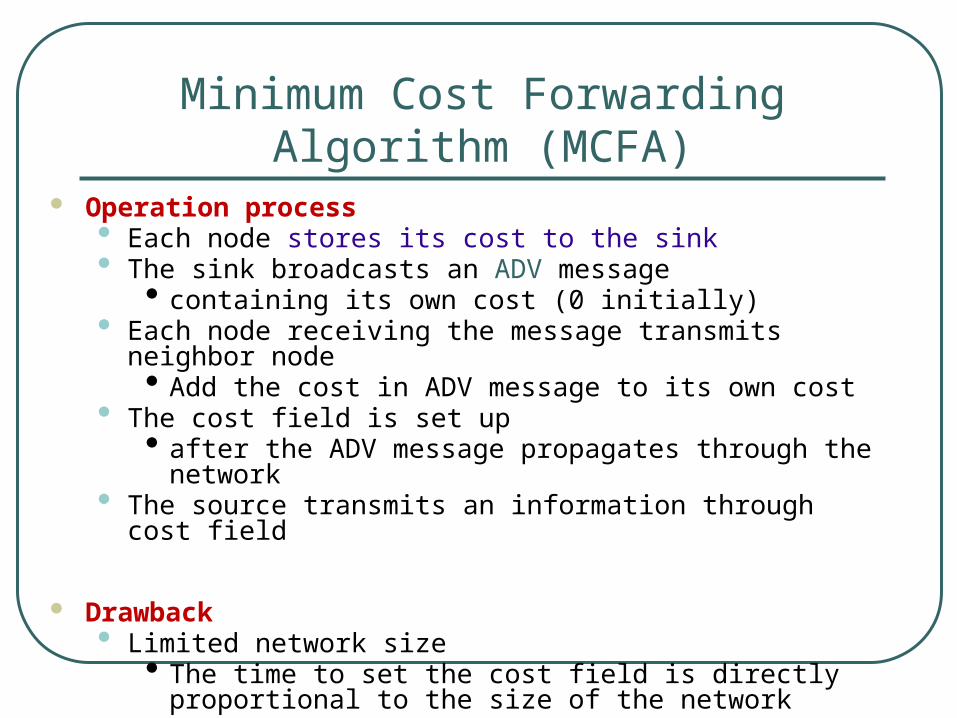
Operation process• Each node stores its cost to the sink• The sink broadcasts an ADV message
• containing its own cost (0 initially)• Each node receiving the message transmits neighbor node
• Add the cost in ADV message to its own cost• The cost field is set up
• after the ADV message propagates through the network• The source transmits an information through cost field
Drawback• Limited network size
• The time to set the cost field is directly proportional to the size of the network
• Load is not balanced
Think…. In Rumor Routing
What about mobile nodes?
What about the multimodal Wireless nodes?
87
Geographic Adaptive Fidelity (GAF)
Forms a virtual grid of the covered area Each node associates itself with a point in the grid
based on its location Nodes associated with same point in grid are
considered equivalent Some nodes in an area are kept sleeping to conserve
energy Nodes change state from sleeping to active for load
balancing
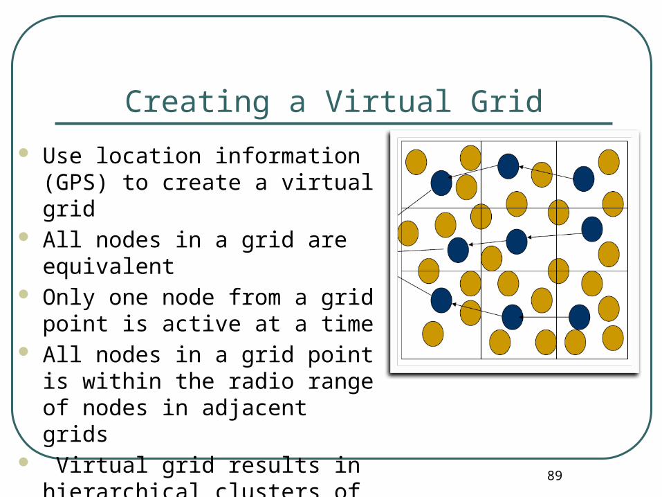
Creating a Virtual Grid
Use location information (GPS) to create a virtual grid
All nodes in a grid are equivalent Only one node from a grid point is
active at a time All nodes in a grid point is within the
radio range of nodes in adjacent grids Virtual grid results in hierarchical
clusters of nodes
89
Think once more ….
What are the problems of GAF?
What about mobile nodes?
What about the multimodal Wireless nodes?
90