Introduction to spectral clustering

Philippe BielaHEI – LAGIS

Philippe.Biela@hei.fr

Denis HamadLASL – ULCO

Denis.Hamad@lasl.univ-littoral.fr

Data Clustering

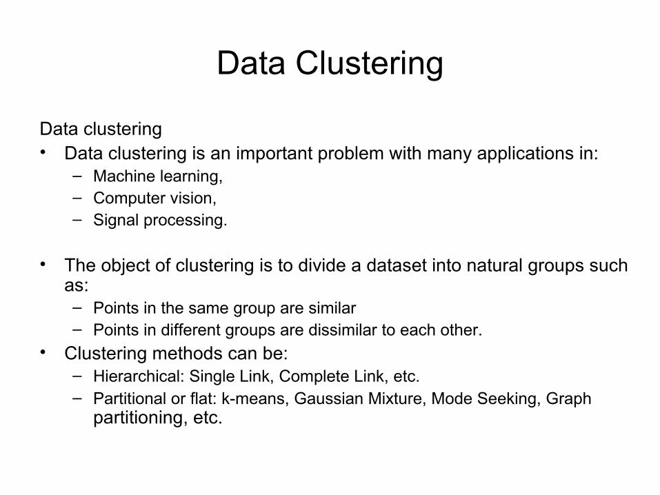
Data clustering • Data clustering is an important problem with many applications in:

– Machine learning, – Computer vision, – Signal processing.

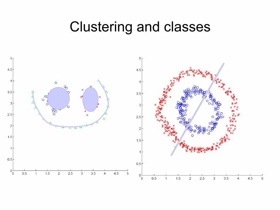
• The object of clustering is to divide a dataset into natural groups such as: – Points in the same group are similar– Points in different groups are dissimilar to each other.

• Clustering methods can be:– Hierarchical: Single Link, Complete Link, etc. – Partitional or flat: k-means, Gaussian Mixture, Mode Seeking, Graph

partitioning, etc.

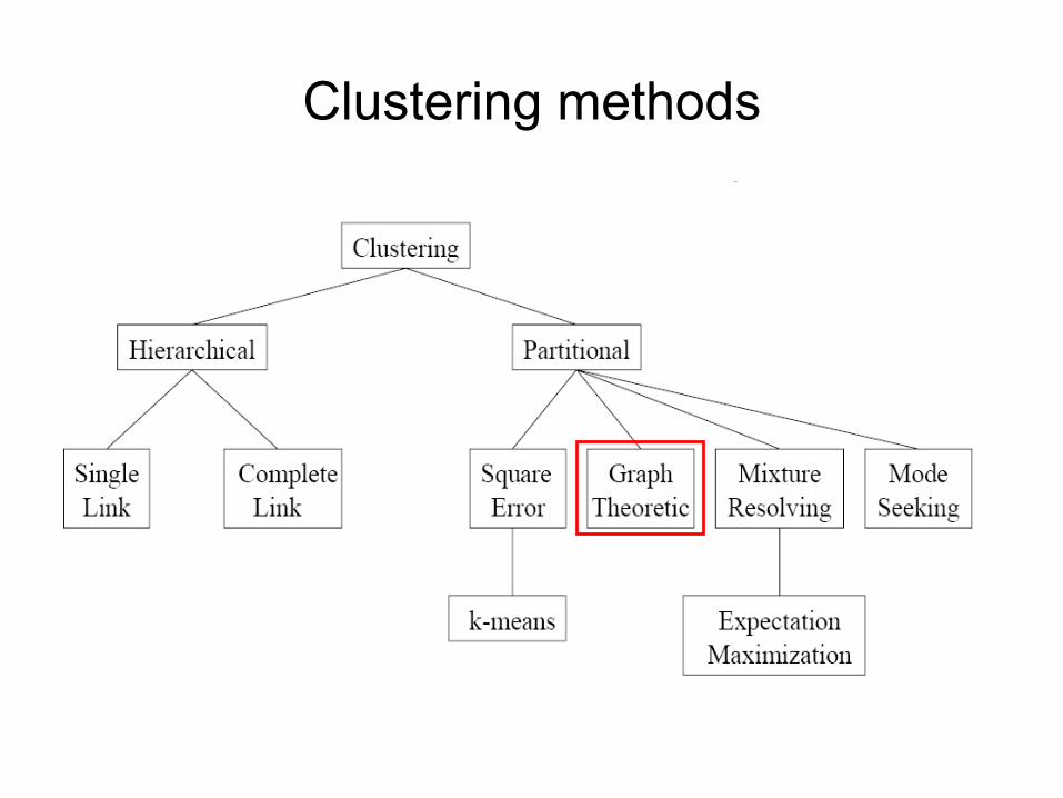
Clustering methods

Clustering and classes

Spectral clustering

Spectral clustering• Spectral clustering methods are attractive:

– Easy to implement, – Reasonably fast especially for sparse data sets up to several

thousands.

• Spectral clustering treats the data clustering as a graph partitioning problem without make any assumption on the form of the data clusters.

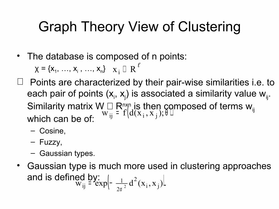
Graph Theory View of Clustering

• The database is composed of n points: χ = {x1, …, xi , …, xn}

∀ Points are characterized by their pair-wise similarities i.e. to each pair of points (xi, xj) is associated a similarity value wij. Similarity matrix W ∈ Rnxn is then composed of terms wij which can be of:– Cosine, – Fuzzy, – Gaussian types.

• Gaussian type is much more used in clustering approaches and is defined by:

ℓRx i ∈

( ))x,x(dexpw ji2

21

ij 2σ−=

( )θ= );x,x(dfw jiij

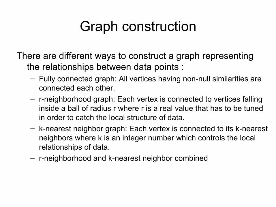
Graph construction

There are different ways to construct a graph representing the relationships between data points :– Fully connected graph: All vertices having non-null similarities are

connected each other. – r-neighborhood graph: Each vertex is connected to vertices falling

inside a ball of radius r where r is a real value that has to be tuned in order to catch the local structure of data.

– k-nearest neighbor graph: Each vertex is connected to its k-nearest neighbors where k is an integer number which controls the local relationships of data.

– r-neighborhood and k-nearest neighbor combined

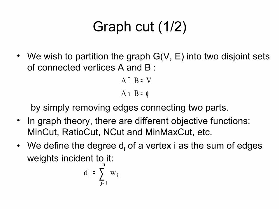
• We wish to partition the graph G(V, E) into two disjoint sets of connected vertices A and B :

by simply removing edges connecting two parts. • In graph theory, there are different objective functions:

MinCut, RatioCut, NCut and MinMaxCut, etc. • We define the degree di of a vertex i as the sum of edges

weights incident to it:

Graph cut (1/2)

φ=∩=∪

BAVBA

∑=

=n

1jiji wd

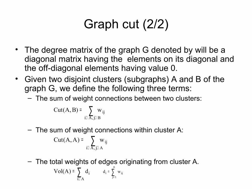
Graph cut (2/2)

• The degree matrix of the graph G denoted by will be a diagonal matrix having the elements on its diagonal and the off-diagonal elements having value 0.

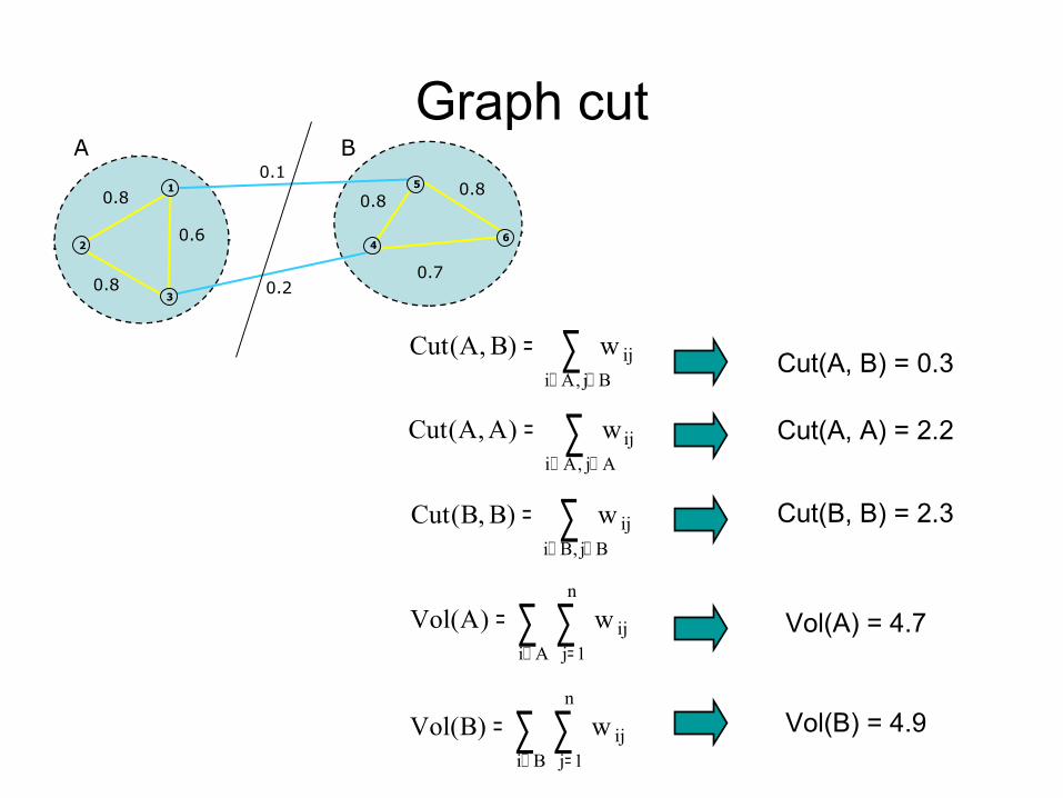
• Given two disjoint clusters (subgraphs) A and B of the graph G, we define the following three terms:– The sum of weight connections between two clusters:

– The sum of weight connections within cluster A:

– The total weights of edges originating from cluster A.

∑∈∈

=Bj,Ai

ijw)B,A(Cut

∑∈∈

=Aj,Ai

ijw)A,A(Cut

∑∈

=Ai

id)A(Vol ∑=

=n

1jiji wd

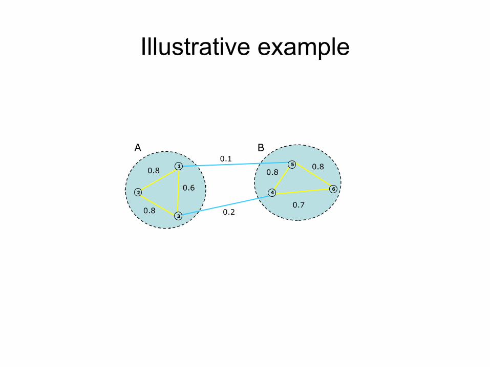
Illustrative example

0.1

0.2

0.8

0.7

0.6

0.8

0.8

1

2

3

4

5

6

0.8

A B

Graph cut0.1

0.2

0.8

0.7

0.6

0.8

0.8

1

2

3

4

5

6

0.8

A B

∑∈∈

=Aj,Ai

ijw)A,A(Cut

∑∈∈

=Bj,Ai

ijw)B,A(Cut

∑∈∈

=Bj,Bi

ijw)B,B(Cut

∑ ∑∈ =

=Ai

n

1jijw)A(Vol

∑ ∑∈ =

=Bi

n

1jijw)B(Vol

Cut(A, B) = 0.3

Cut(A, A) = 2.2

Cut(B, B) = 2.3

Vol(A) = 4.7

Vol(B) = 4.9

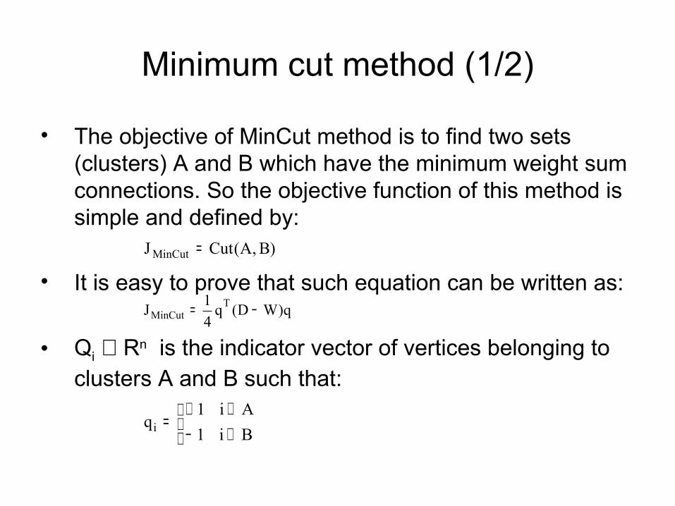
• The objective of MinCut method is to find two sets (clusters) A and B which have the minimum weight sum connections. So the objective function of this method is simple and defined by:

• It is easy to prove that such equation can be written as:

• Qi ∈ Rn is the indicator vector of vertices belonging to clusters A and B such that:

)B,A(CutJ MinCut =

q)WD(q41J T

MinCut −=

∈−∈+

=Bi1Ai1

qi

Minimum cut method (1/2)

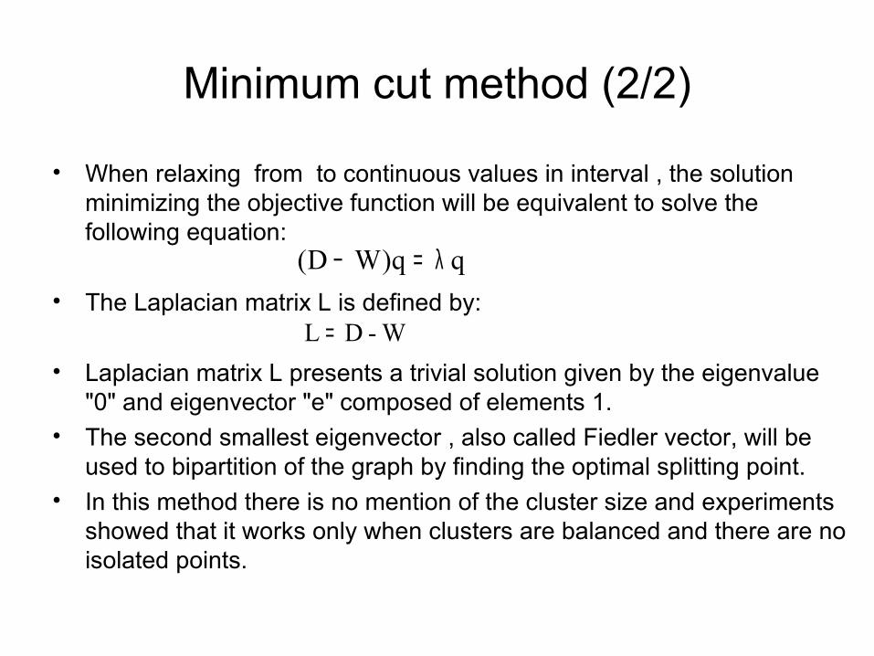
• When relaxing from to continuous values in interval , the solution minimizing the objective function will be equivalent to solve the following equation:

• The Laplacian matrix L is defined by:

• Laplacian matrix L presents a trivial solution given by the eigenvalue "0" and eigenvector "e" composed of elements 1.

• The second smallest eigenvector , also called Fiedler vector, will be used to bipartition of the graph by finding the optimal splitting point.

• In this method there is no mention of the cluster size and experiments showed that it works only when clusters are balanced and there are no isolated points.

qq)WD( λ=−

W- D L =

Minimum cut method (2/2)

Ratio cut method

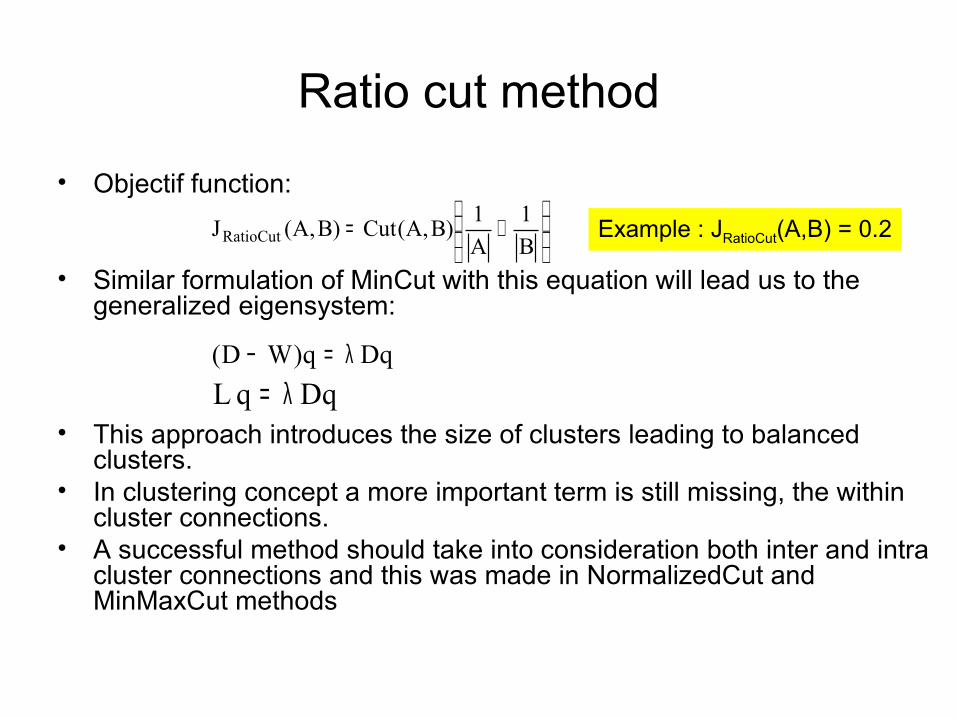
• Objectif function:

• Similar formulation of MinCut with this equation will lead us to the generalized eigensystem:

• This approach introduces the size of clusters leading to balanced clusters.

• In clustering concept a more important term is still missing, the within cluster connections.

• A successful method should take into consideration both inter and intra cluster connections and this was made in NormalizedCut and MinMaxCut methods

+=

B1

A1)B,A(Cut)B,A(JRatioCut

Dqq)WD( λ=−DqqL λ=

Example : JRatioCut(A,B) = 0.2

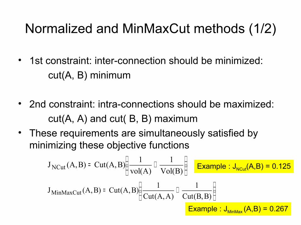
Normalized and MinMaxCut methods (1/2)

• 1st constraint: inter-connection should be minimized:cut(A, B) minimum

• 2nd constraint: intra-connections should be maximized:cut(A, A) and cut( B, B) maximum

• These requirements are simultaneously satisfied by minimizing these objective functions

+=

)B(Vol1

)A(vol1)B,A(Cut)B,A(J NCut

+=

)B,B(Cut1

)A,A(Cut1)B,A(Cut)B,A(JMinMaxCut

Example : JNCut(A,B) = 0.125

Example : JMinMax (A,B) = 0.267

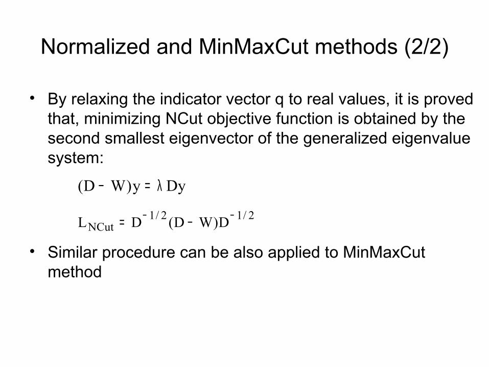
Normalized and MinMaxCut methods (2/2)

• By relaxing the indicator vector q to real values, it is proved that, minimizing NCut objective function is obtained by the second smallest eigenvector of the generalized eigenvalue system:

• Similar procedure can be also applied to MinMaxCut method

Dyy)WD( λ=−

2/12/1NCut D)WD(DL −− −=

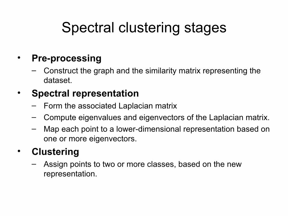
Spectral clustering stages

• Pre-processing– Construct the graph and the similarity matrix representing the

dataset.• Spectral representation

– Form the associated Laplacian matrix – Compute eigenvalues and eigenvectors of the Laplacian matrix.– Map each point to a lower-dimensional representation based on

one or more eigenvectors.• Clustering

– Assign points to two or more classes, based on the new representation.

Illustrative example

0.1

0.2

0.8

0.7

0.6

0.8

0.8

1

2

3

4

5

6

0.8

A B

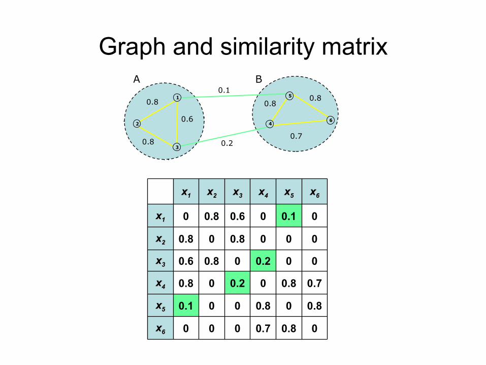
00.80.7000xx66

0.800.8000.1xx55

0.70.800.200.8xx44

000.200.80.6xx33

0000.800.8xx22

00.100.60.80xx11

xx66xx55xx44xx33xx22xx11

Graph and similarity matrix0.1

0.2

0.8

0.7

0.6

0.8

0.8

1

2

3

4

5

6

0.8

A B

Illustrative example

x6

x5

x4

x3

x2

x1

1.5-0.8-0.7000

-0.81.70.800-0.1

-0.7-0.82.5-0.20-0.8

00-0.21.6-0.8-0.6

000-0.81.6-0.8

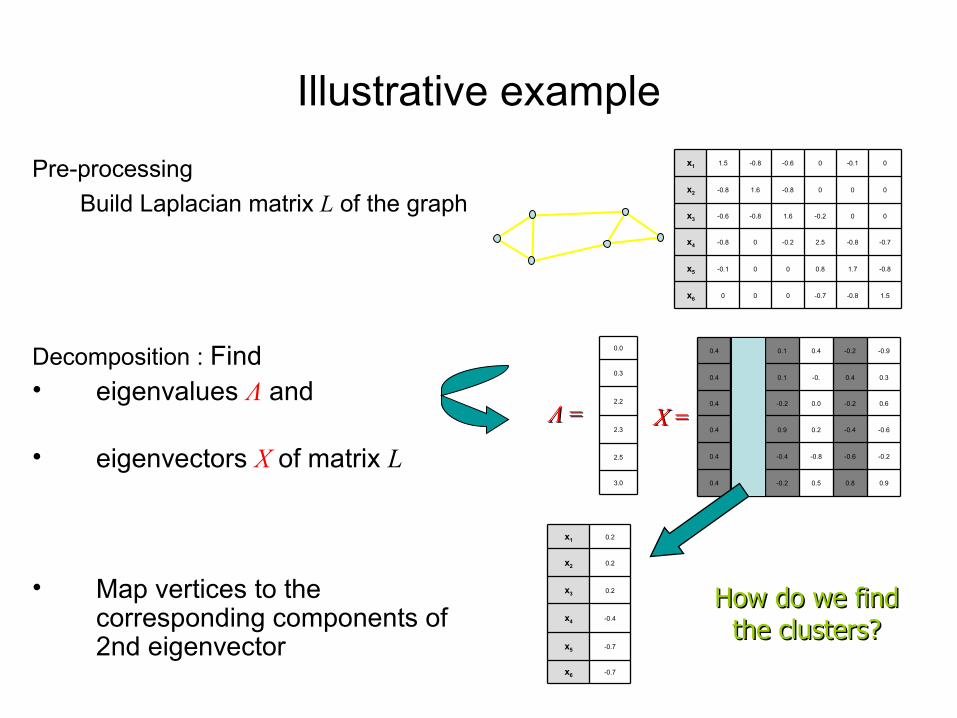
0-0.10-0.6-0.81.5Pre-processingBuild Laplacian matrix L of the graph

0.90.80.5-0.2-0.70.4

-0.2-0.6-0.8-0.4-0.70.4

-0.6-0.40.20.9-0.40.4

0.6-0.20.0-0.20.20.4

0.30.4-0.0.10.20.4

-0.9-0.20.40.10.20.4

3.0

2.5

2.3

2.2

0.3

0.0

ΛΛ = = XX = =

Decomposition : Find • eigenvalues Λ and

• eigenvectors X of matrix L

• Map vertices to the corresponding components of 2nd eigenvector

How do we find How do we find the clusters?the clusters?

-0.7x6

-0.7x5

-0.4x4

0.2x3

0.2x2

0.2x1

Spectral Clustering Algorithms (continued)

-0.7x6

-0.7x5

-0.4x4

0.2x3

0.2x2

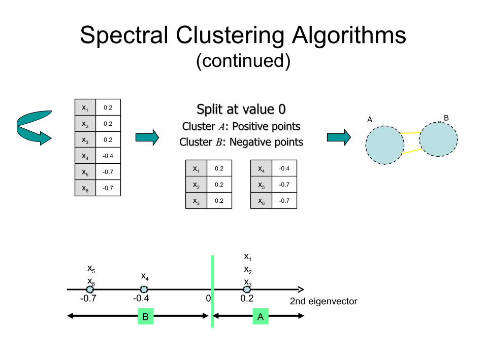
0.2x1 Split at value 0Split at value 0Cluster Cluster AA: Positive points: Positive pointsCluster Cluster BB: Negative points: Negative points

0.2x3

0.2x2

0.2x1

-0.7x6

-0.7x5

-0.4x4

A B

0 0.2-0.4-0.7

x5

x6x4

x1

x2

x3

2nd eigenvector

AB

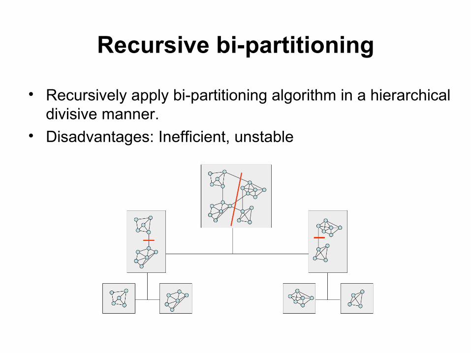
Recursive bi-partitioning

• Recursively apply bi-partitioning algorithm in a hierarchical divisive manner.

• Disadvantages: Inefficient, unstable

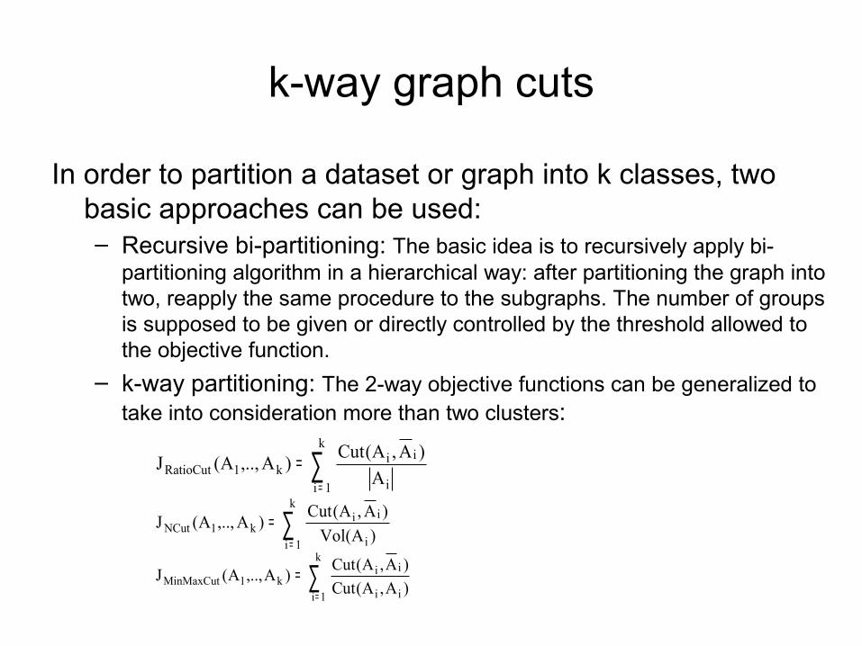
k-way graph cuts

In order to partition a dataset or graph into k classes, two basic approaches can be used:– Recursive bi-partitioning: The basic idea is to recursively apply bi-

partitioning algorithm in a hierarchical way: after partitioning the graph into two, reapply the same procedure to the subgraphs. The number of groups is supposed to be given or directly controlled by the threshold allowed to the objective function.

– k-way partitioning: The 2-way objective functions can be generalized to take into consideration more than two clusters:

∑=

=k

1i i

iik1RatioCut A

)A,A(Cut)A,..,A(J

∑=

=k

1i i

iik1NCut )A(Vol

)A,A(Cut)A,..,A(J

∑=

=k

1i ii

iik1MinMaxCut )A,A(Cut

)A,A(Cut)A,..,A(J

Spectral clustering stages

• Pre-processing– Construct the graph and the similarity matrix representing the

dataset.• Spectral representation

– Form the associated Laplacian matrix – Compute eigenvalues and eigenvectors of the Laplacian matrix.– Map each point to a lower-dimensional representation based on

one or more eigenvectors.• Clustering

– Assign points to two or more classes, based on the new representation.

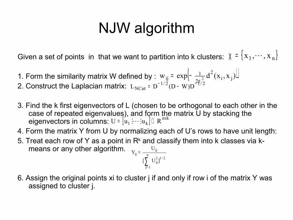
NJW algorithm

Given a set of points in that we want to partition into k clusters:

1. Form the similarity matrix W defined by : 2. Construct the Laplacian matrix:

3. Find the k first eigenvectors of L (chosen to be orthogonal to each other in the case of repeated eigenvalues), and form the matrix U by stacking the eigenvectors in columns:

4. Form the matrix Y from U by normalizing each of U’s rows to have unit length:5. Treat each row of Y as a point in Rk and classify them into k classes via k-

means or any other algorithm.

6. Assign the original points xi to cluster j if and only if row i of the matrix Y was assigned to cluster j.

{ }n1 x,,x ⋯=χ

( ))x,x(dexpw ji2

21

ij 2σ−=

2/12/1NCut D)WD(DL −− −=

[ ] nxkk1 RuuU ∈= ⋮⋯⋮

2/1n

1j

2ij

ijij

]U[

UY

∑=

=

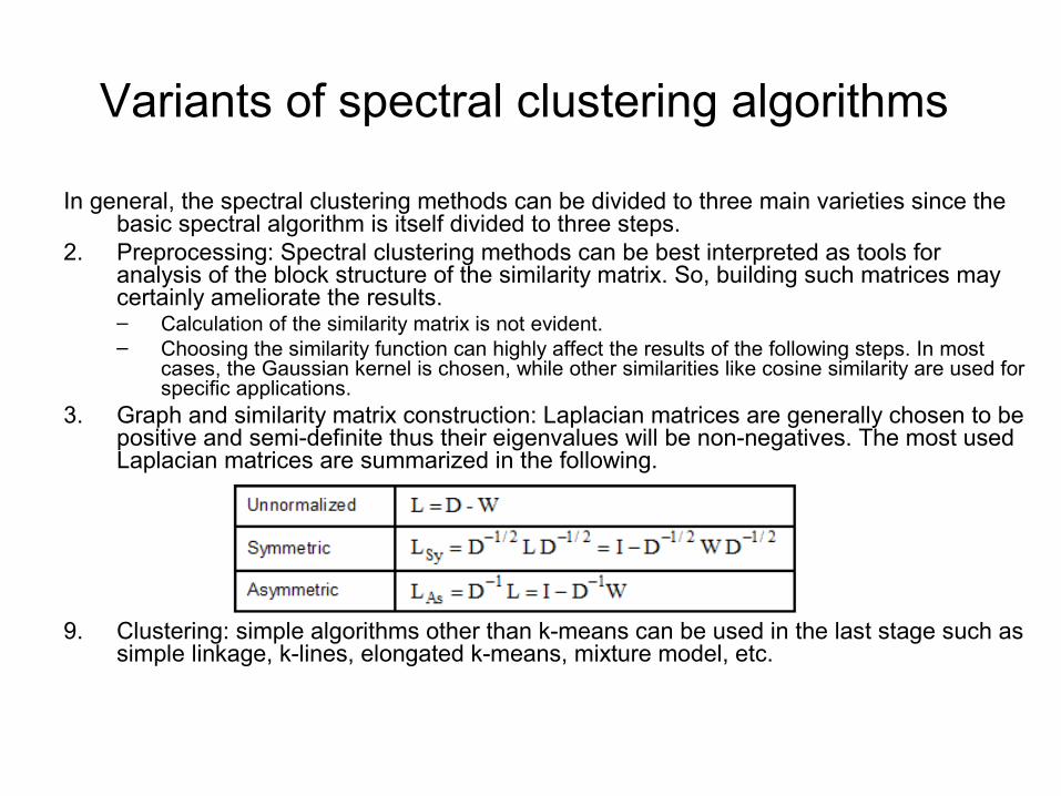
Variants of spectral clustering algorithms

In general, the spectral clustering methods can be divided to three main varieties since the basic spectral algorithm is itself divided to three steps.

2. Preprocessing: Spectral clustering methods can be best interpreted as tools for analysis of the block structure of the similarity matrix. So, building such matrices may certainly ameliorate the results. – Calculation of the similarity matrix is not evident.– Choosing the similarity function can highly affect the results of the following steps. In most

cases, the Gaussian kernel is chosen, while other similarities like cosine similarity are used for specific applications.

3. Graph and similarity matrix construction: Laplacian matrices are generally chosen to be positive and semi-definite thus their eigenvalues will be non-negatives. The most used Laplacian matrices are summarized in the following.

9. Clustering: simple algorithms other than k-means can be used in the last stage such as simple linkage, k-lines, elongated k-means, mixture model, etc.

Parameters tuning (1/2)

• The free parameter of Gaussian kernel is often overlooked. Indeeed, with different values of σ, the results of clustering can be vastly different.

• The parameter is done manually. • The parameter is selected automatically by running the spectral algorithm

repeatedly for a number of values and selecting the one which provides least distorted clusters in spectral representation space.

Weakness of this method: – computation time, – the range of values to be tested has to be set manually – with input data including clusters with different local statistics there may not be a

single value of that works well for all the data.

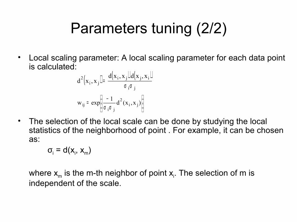
Parameters tuning (2/2)

• Local scaling parameter: A local scaling parameter for each data point is calculated:

• The selection of the local scale can be done by studying the local statistics of the neighborhood of point . For example, it can be chosen as:

σi = d(xi, xm)

where xm is the m-th neighbor of point xi. The selection of m is independent of the scale.

( ) ( ) ( )ji

ijjiji

2 x,xdx,xdx,xd

σσ=

σσ−= )x,x(d1expw ji

2

jiij

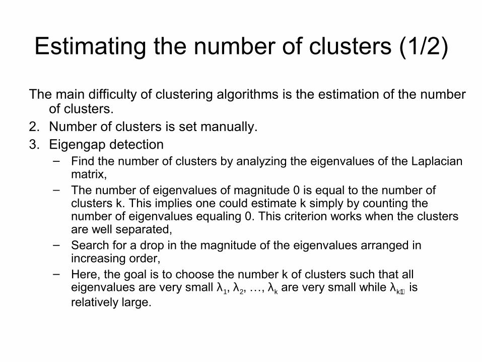
Estimating the number of clusters (1/2)

The main difficulty of clustering algorithms is the estimation of the number of clusters.

2. Number of clusters is set manually. 3. Eigengap detection

– Find the number of clusters by analyzing the eigenvalues of the Laplacian matrix,

– The number of eigenvalues of magnitude 0 is equal to the number of clusters k. This implies one could estimate k simply by counting the number of eigenvalues equaling 0. This criterion works when the clusters are well separated,

– Search for a drop in the magnitude of the eigenvalues arranged in increasing order,

– Here, the goal is to choose the number k of clusters such that all eigenvalues are very small λ1, λ2, …, λk are very small while λk+1 is relatively large.

Estimating the number of clusters (2/2)

• Find canonical coordinate system:– Minimize the cost of aligning the top eigenvectors with a canonical

coordinate system. – The search can be performed incrementally. – At each step of the search, a single eigenvector is added to the

already rotated ones. – This can be viewed as taking the alignment results of the previews

number as an initialization to the current one

Application of spectral clustering inSignal and image processing

Signal processing

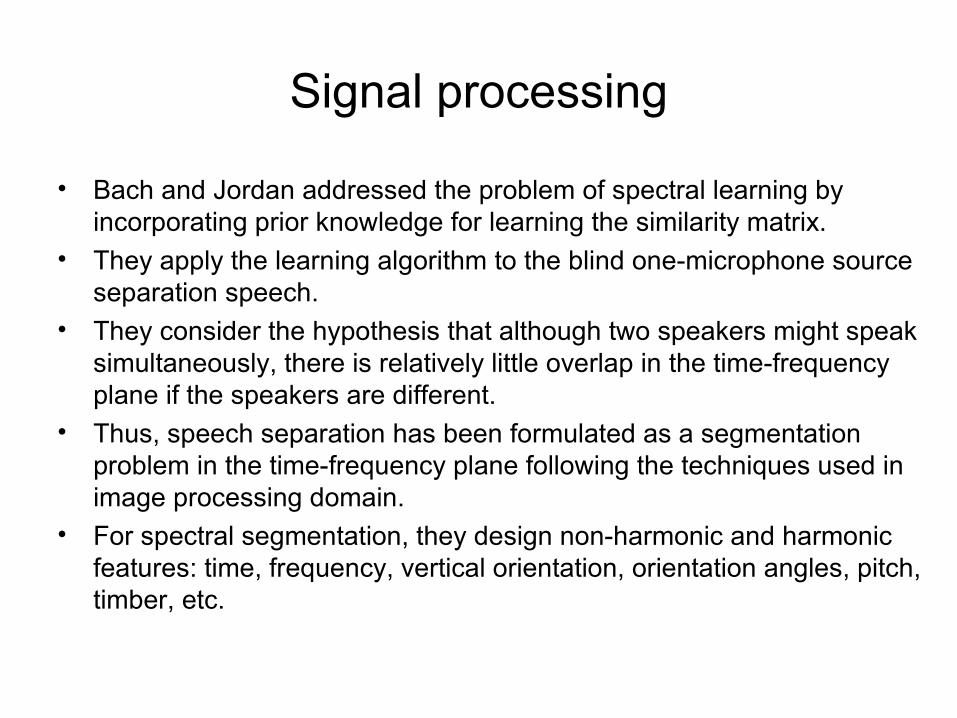
• Bach and Jordan addressed the problem of spectral learning by incorporating prior knowledge for learning the similarity matrix.

• They apply the learning algorithm to the blind one-microphone source separation speech.

• They consider the hypothesis that although two speakers might speak simultaneously, there is relatively little overlap in the time-frequency plane if the speakers are different.

• Thus, speech separation has been formulated as a segmentation problem in the time-frequency plane following the techniques used in image processing domain.

• For spectral segmentation, they design non-harmonic and harmonic features: time, frequency, vertical orientation, orientation angles, pitch, timber, etc.

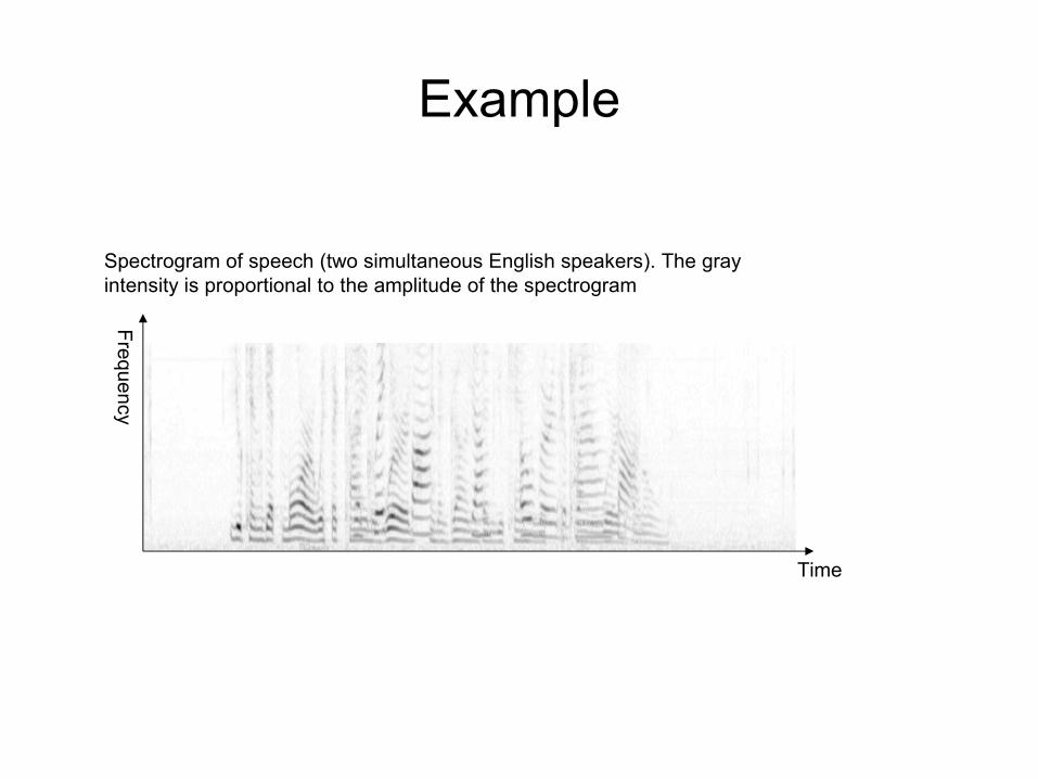
Example

Spectrogram of speech (two simultaneous English speakers). The gray intensity is proportional to the amplitude of the spectrogram

Time

Frequency

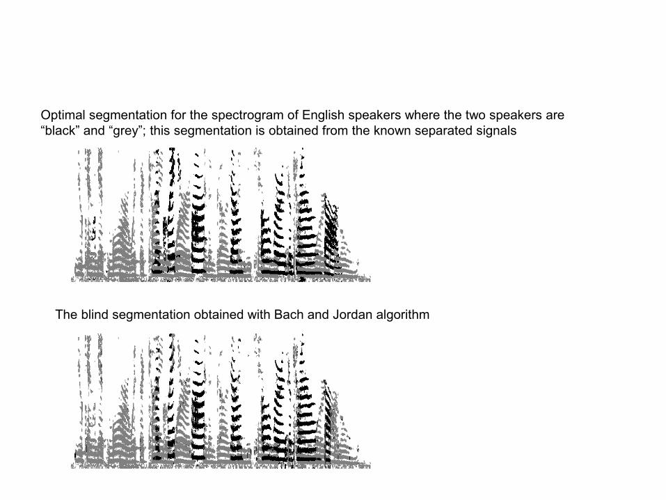
Optimal segmentation for the spectrogram of English speakers where the two speakers are “black” and “grey”; this segmentation is obtained from the known separated signals

The blind segmentation obtained with Bach and Jordan algorithm

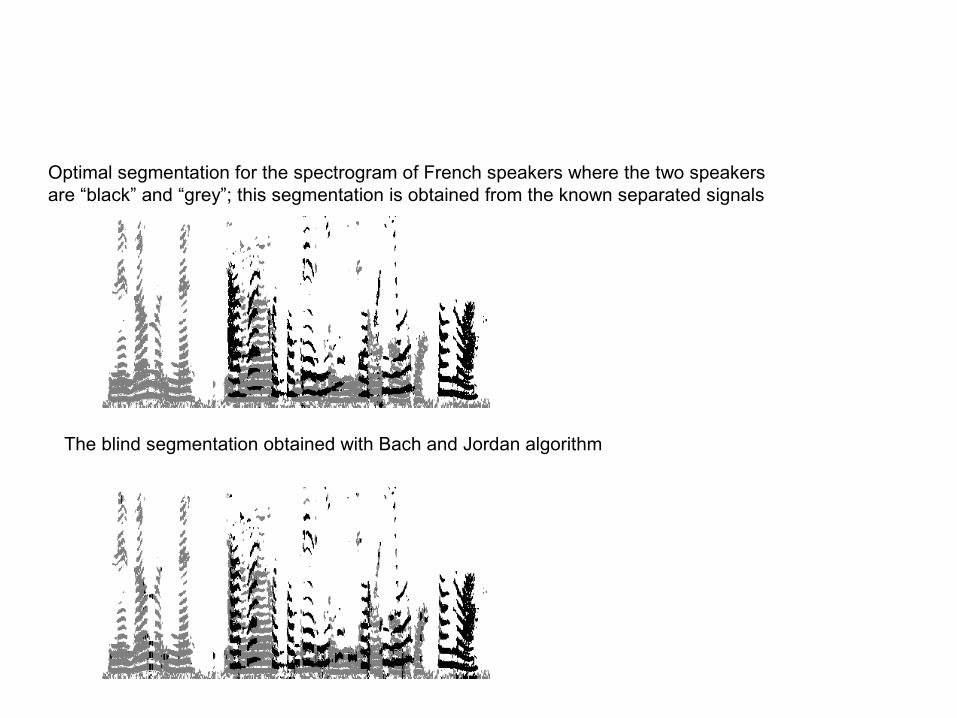
Optimal segmentation for the spectrogram of French speakers where the two speakers are “black” and “grey”; this segmentation is obtained from the known separated signals

The blind segmentation obtained with Bach and Jordan algorithm

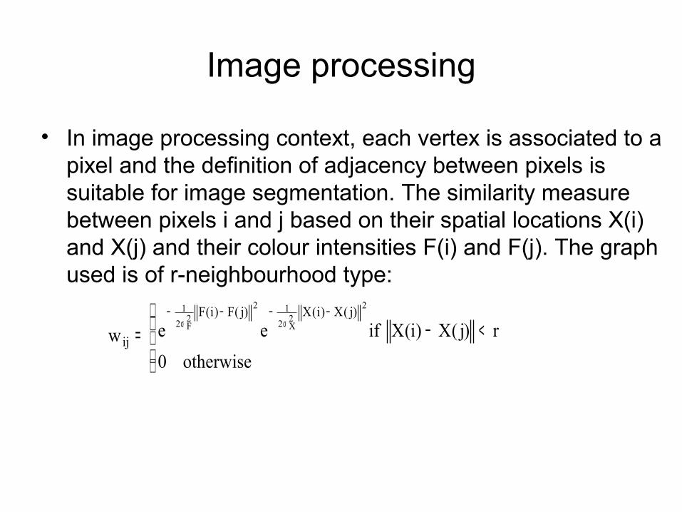
Image processing

• In image processing context, each vertex is associated to a pixel and the definition of adjacency between pixels is suitable for image segmentation. The similarity measure between pixels i and j based on their spatial locations X(i) and X(j) and their colour intensities F(i) and F(j). The graph used is of r-neighbourhood type:

<−=−−−−

σσ

otherwise0r)j(X)i(Xifeew

22X2

122F2

1 )j(X)i(X)j(F)i(F

ij

Examples

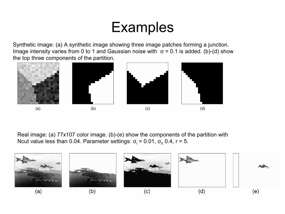
Real image: (a) 77x107 color image. (b)-(e) show the components of the partition with Ncut value less than 0.04. Parameter settings: σI = 0.01, σX 0.4, r = 5.

Synthetic image: (a) A synthetic image showing three image patches forming a junction. Image intensity varies from 0 to 1 and Gaussian noise with σ = 0.1 is added. (b)-(d) show the top three components of the partition.

Computation and memory problems (1/2)

• Image processing: a small 256x256 gray level image leads to a data set of 65536 points

• Signal processing: 3 seconds of speech sampled at 5kH leads to more than 15000 spectrogram samples.

• Thus, the full similarity matrix having n2 dimensions cannot be stored in main memory. Therefore, techniques which reduce the storage capacity will be very helpful.

Computation and memory problems (2/2)

In signal and image processing domains, similarity matrix grows as the square of the number of elements in the dataset, it quickly becomes infeasible to fit in memory. Then, the need to solve eigensystem presents a serious computational problem.

• Sparse similarity matrix: One approach to deal with this problem is to use a sparse, approximate version of similarity in which each element is connected only to a few of its nearby neighbors and all other connections are assumed to be zero. – Employ efficient eigensolvers: Lanczos iterative approach.

• Nyström method: Numerical solution of eigenfunction problem. This method allows one to extrapolate the complete grouping solution using only a small random number of samples. In doing so, we leverage the fact that there are far fewer coherent groups in a scene than pixels

Conclusion

• Some spectral clustering methods are presented.• They can be divided into three categories according to the basic

stages of standard spectral clustering: – pre-processing, – spectral representation,– clustering.

• We pointed out various solutions to their main problems: – parameters tuning,– number of clusters estimation,– complexity computation.

• The success of spectral methods is due to their capacity to discover the data clusters without any assumption about their statistics.

• For these reasons, they are recently applied in different domains particularly in signal and image processing.

Bibliography• Bach F. R. and M. I. Jordan, “Learning spectral clustering, with application to speech separation”, Journal of Machine Learning Research,

vol. 7, pp. 1963-2001, 2006.• Bach F. R. and M. I. Jordan, “Learning spectral clustering”, In Thrun S. and Soul L. editors. NIPS’16, Cambridge, MA, MIT Press, 2004.• Chang H., D.-Y. Yeung, “Robust path-based spectral clustering”, Pattern Recognition 41 (1), pp. 191-203, 2008.• Ding C., X. H. He, Zha, M. Gu, and H. Simon, “A min-max cut algorithm for graph partitioning and data clustering”. IEEE first Conference on

Data Mining, pp. 107-114, 2001.• Fowlkes C., S. Belongie, F. Chung, and J. Malik, “Spectral Grouping Using the Nyström Method”, IEEE Trans. on Pattern Analysis and

Machine Intelligence, vol. 26, no. 2, pp. 214-225, 2004.• Hagen L. and A. Kahng, “Fast spectral methods for ratio cut partitioning and clustering”. In Proceedings of IEEE International Conference on

Computer Aided Design, pp. 10-13, 1991.• Jain A., M. N. Murty and P. J. Flynn “Data clustering: A review”. ACM Computing Surveys, vol. 31(3), pp. 264-323, 1999.• Meila M. and L. Xu, “Multiway cuts and spectral clustering”, Advances in Neural Information Processing Systems, 2003.• Ng, A. Y., M. I., Jordan, and Y. Weiss, “On spectral clustering: Analysis and an algorithm”. Advances in Neural Information Processing

Systems 14, volume 14, pp. 849-856, 2002. • Sanguinetti G., J. Laidler, and N. D. Lawrence. "Automatic determination of the number of clusters using spectral algorithms", IEEE Machine

Learning for Signal Processing conference, Mystic, Connecticut, USA, 28-30 september, 2005. • Shi. J. and J. Malik. "Normalized cuts and image segmentation", IEEE Trans. on Pattern Analysis and Machine Intelligence, vol. 22, no 8, pp.

888-905, 2000.• von Luxburg U., “A tutorial on spectral clustering”, Technical report, No TR-149, Max-Planck-Institut für biologische Kybernetik, 2007.• Xiang T. S. Gong, “Spectral clustering with eigenvector selection”, Pattern Recognition, vol. 41, no 3, pp. 1012-1029, 2008.• Yu S.X. and J. Shi “Multiclass spectral clustering” 9th IEEE International Conference on Computer Vision CCV, Washinton, DC, USA, 2003.• Yu S.X., J. Shi, Segmentation given partial grouping constraints, IEEE Trans. on Pattern Analysis and Machine Intelligence, vol. 26, no 2, pp.

173–183, 2004.• Zelnik-Manor L., P. Perona, “Self-Tuning spectral clustering”, Advances in Neural Information Processing Systems, vol. 17, 2005.• Derek greene, "Graph partitioning and spectral clustering", https://www.cs.tcd.ie/research_groups/mlg/kdp/presentations/Greene_MLG04.ppt