Inventory Control - POMS

Prod 2100-2110 Inventory Control 0

Inventory Control

� When to order ? � How many to order ?

Contents

1. FRAMEWORK OF PLANNING DECISIONS...............................................................................1

2. INVENTORY CONTROL.................................................................................................................2

2.1 CONTROL SYSTEMS .............................................................................................................................3 2.2 PARAMETERS ......................................................................................................................................4 2.3 COSTS..................................................................................................................................................5

3. INVENTORY CONTROL: DETERMINISTIC MODEL..............................................................6

3.1 WILSON'S MODEL OR THE EOQ MODEL .............................................................................................6 3.2 EOQ: MARGINAL ANALYSIS.................................................................................................................9 3.3 EOQ: EXAMPLES AND SENSITIVITY....................................................................................................10 3.4 EOQ WITH POSITIVE LEAD TIME........................................................................................................11 3.5 EOQ WITH FINITE PRODUCTION RATE ................................................................................................12 3.6 EOQ WITH DISCOUNT ON ALL UNITS .................................................................................................13 3.7 EOQ WITH INCREMENTAL DISCOUNT.................................................................................................16 3.8 ECONOMIC REPLENISHMENT INTERVAL ............................................................................................18

4 INVENTORY CONTROL: STOCHASTIC MODELS .................................................................19

4.1 RANDOM DEMAND ............................................................................................................................19 4.2 LOT SIZE - REORDER POINT MODEL OR (Q, R) MODEL ......................................................................21 4.3 OBJECTIVE 1: STOCKOUT PROBABILITY ............................................................................................23 4.4 OBJECTIVE 2: FILL RATE (SERVICE LEVEL)........................................................................................28 4.5 OBJECTIVE 3: MINIMIZE THE TOTAL COSTS........................................................................................31 4.6 PERIODIC REVIEW SYSTEMS ..............................................................................................................33 4.7 LEAD TIME VARIABILITY...................................................................................................................37

5. MULTIPRODUCT SYSTEMS: ABC ANALYSIS........................................................................38

Silver E.A. and R.Peterson, Decision Systems for Inventory Management and Production Planning, Second Edition, John Wiley & Sons, 1995.


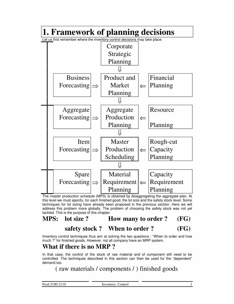
1. Framework of planning decisions Let us first remember where the inventory control decisions may take place.

Corporate Strategic Planning

� Business

Forecasting �

Product and Market

Planning

⇐

Financial Planning

� Aggregate

Forecasting �

Aggregate Production Planning

⇐

Resource Planning

� Item

Forecasting �

Master Production Scheduling

⇐

Rough-cut Capacity Planning

� Spare

Forecasting �

Material Requirement

Planning

⇐

Capacity Requirement Planning

The master production schedule (MPS) is obtained by disaggregating the aggregate plan. At this level we must specify, for each finished good, the lot size and the safety stock level. Some techniques for lot sizing have already been proposed in the previous section. Here we will address this problem more globally. The problem of choosing the safety stock was not yet tackled. This is the purpose of this chapter.

MPS: lot size ? How many to order ? (FG)

safety stock ? When to order ? (FG) Inventory control techniques thus aim at solving the two questions : “When to order and how much ?” for finished goods. However, not all company have an MRP system.

What if there is no MRP ? In that case, the control of the stock of raw material and of component still need to be controlled. The techniques described in this section can then be used for the “dependent” demand too.

( raw materials / components / ) finished goods


2. Inventory Control Here are several examples which illustrates the ins and outs of the inventory control. These examples are drawn from the daily life. Try to find the rational which hides behind each situation.

Examples : buying coffee / filters Let's refer to our Makecoffee example again. How often do you buy coffee and filters? Don't you buy coffee more often than filters? Why? What are the reasons for that?

going to the department store Where do you make your shopping? Do you go to the department store where you buy everything or to different specialized shops (bakery, butcher, ...)? Why?

buying cigarettes / breads The smokers usually buy their cigarettes on a daily basis. Why? Are there situations where big lots are bought at once? What about buying breads ?

washing the dishes Usually, the dishes are washed after each meal, sometimes once a day, seldom once a week. Why don't we clean each dish after we used it?

Factors : setup �� order in big lots Going to the store is a setup operation. Prepare the water for washing the dishes is a setup too. When preparing pancakes, the first one we scrap because it’s too oily is a setup too. When ordering things, the preparation of the order (paper work, calls), its transport and its reception can all be seen as setup operations whose cost is fixed and independent of the quantity which is bought. When launching a production order, the preparation of the environment (raw material), the setup of the machines and the first items that are scrapped for quality reasons can all be seen as setup operations whose costs are fixed and independent of the quantity which is then produced. The cost associated to the setup operations favors ordering in big lots.

capital �� order in small lots Coffee is more expensive than filters. Cigarettes are very expensive. Nobody wants to invest money too early if it is not necessary. By delaying the investments, the money can be used in the mean time, possibly for generating interests. The money which is invested in goods (coffee, cigarettes) has thus a cost: the loss of the return which could have been made if the money was available. This cost is called opportunity cost of the money. It depends on the opportunities you have ? This cost favors ordering as late as possible and just what is needed (in small lots). This applies to purchasing (raw material) and production (finished goods) similarly.

depreciation �� order in small lots Filters and cigarettes do not get bad. They could remain a long time in our inventory. Coffee does get bad, breads too. We do not buy them in big quantities. The risk that things get bad, out-of-date, deteriorated or obsolete favors building low inventories, that is, ordering as late as possible and as few as possible (small lots). This is valid for raw material and for finished goods.

shortage risk �� keep a safety stock We buy many things (bread, cigarette, wine) before the weekend in case of. Because many shops close during the weekend, we loose the possibility of buying things just when they are needed. We cannot get immediately, that is in zero time, what we want. The delay between the moment we want something and order it and the moment we receive the order is called the "order lead time". When the order lead time in not zero and when the demand is not exactly known, there is a risk of falling short. In order to balance this risk, a safety stock can be built.


2.1 Control Systems

Motivation for holding inventories Here we summarize all the reasons which could justify the creation of an inventory.

1. economy of scale The first motivation is related to the notion of setup discussed on the previous page.

2. uncertainty of demand, of delivery, of price The second main reason is related to the notion of shortage risk also discussed above.

3. smoothing demand over time Building inventory is a possible solution to meet a demand which varies over time with a constant production force. The aggregate planning is a clear illustration of this concept.

4. flexibility in planning !!! An inventory of finished goods allows you to modify the production plan as needed. However the same flexibility can most often be reached by a more efficient way.

Motivation for not holding inventories The two first aspects were discussed on the previous page.

1. capital 2. depreciation - obsolescence - quality 3. flow time

This last aspect is very important. A large inventory can be seen as a large buffer. Considering the production plant as a whole, this large buffer increases the flow time and has therefore many disadvantages.

Decisions Here are the questions we will try to solve in this chapter.

�� When to order? �� How much - how many to order ?

We will consider different control policies.

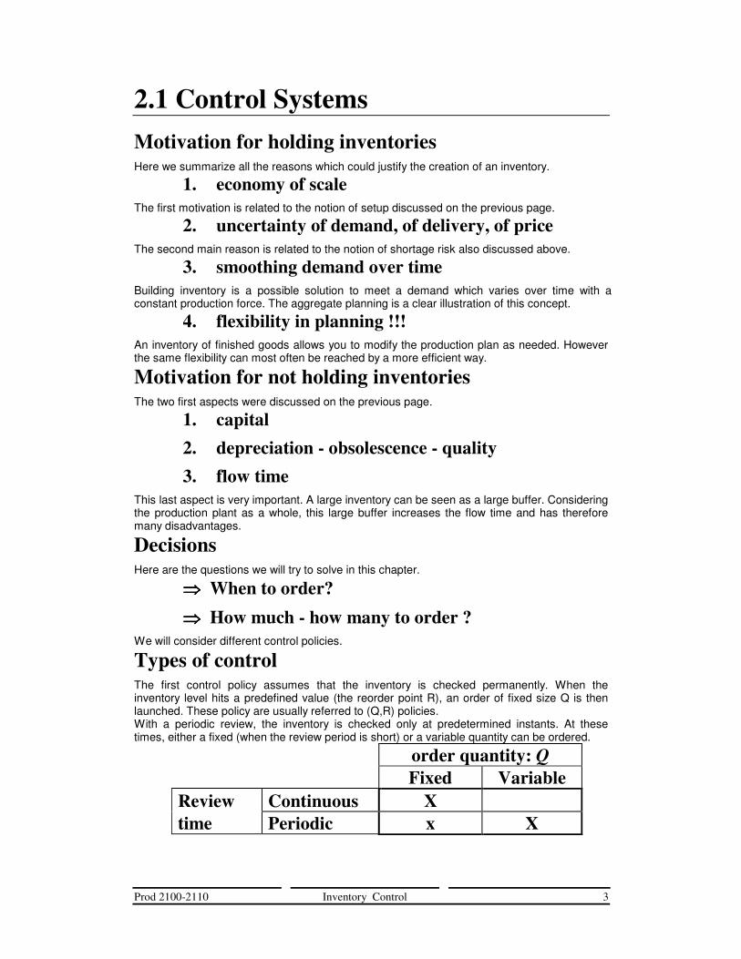
Types of control The first control policy assumes that the inventory is checked permanently. When the inventory level hits a predefined value (the reorder point R), an order of fixed size Q is then launched. These policy are usually referred to (Q,R) policies. With a periodic review, the inventory is checked only at predetermined instants. At these times, either a fixed (when the review period is short) or a variable quantity can be ordered.

order quantity: Q Fixed Variable Review Continuous X time Periodic x X


2.2 Parameters Before trying to build any model for controlling the inventories, let us first review and formalize all the actors of the play.

Demand D ( item / time ) The first data is the demand. The choice of the time unit is arbitrary, but it must be clear. We will consider different kinds of demand.

constant / variable A demand equal to 100 items per month, for each month, is said to be constant. A known demand of 100 items for January, 200 items for February and 150 for March is said to be variable. When computing the aggregated plan, a variable demand was considered.

random (σ≠0) / deterministic (σ= 0) The demand is said to be deterministic if it does not admit any variation. If the monthly demand is 100 items, then it will be 100 each month if it is deterministic. Otherwise, the demand is random and the value 100 gives only the average demand. In this section, we will consider constant demand only, with deterministic or random distribution. Variable demand is considered when considering other lot sizing techniques. We will always use σ to denote the standard deviation of the demand.

Lead time Lt ( time ) The lead time is defined as the time between the moment an order is placed (at a supplier or at a shop) and the moment the items are delivered. It could also be random.

time between order and reception If you order from a supplier, the lead time comprises at least the order processing time, the picking and packing time, the transport time and the reception time. Must also be added all the waiting times: for the picking and packing and for the transport. If your supplier is short of the items you ordered, you must also add the time for replenishing the inventory of the supplier. If you launch a production order, the lead time comprises at least the picking of all the raw materials, the waiting time in front of the first shop, the processing time of the complete lot in the shop, the waiting for transportation facilities and the transportation to the stores. Note that the cycle ( waiting time in front of a shop, processing time in the shop, waiting for transport and transport ) must be accounted for each visited shop.

Review time : Rt ( time ) time between two checking points

With permanent review, the inventory is checked permanently, that is an order decision can be placed at any time. This could be too expensive. A cheaper solution consists in checking the inventory periodically only. The review time is the time between two successive checks. If you check only every Friday, then Rt = 1 week.

unsatisfied demand What happens to the orders which cannot be satisfied must be clearly specified. If there is no more inventory when an order is placed, the customer can just go to another shop. This is the lost sales model. He could also wait patiently for the items to arrive. This is the backorder model. Intermediate models exist where the customers loose patience with time. In each model, an unsatisfied demand generates a cost.

lost / customer impatience / backorder


2.3 Costs When dealing with inventories, three different types of costs are taken into account.

1. Holding cost H money/(item ×××× time) The holding costs are all the cost incurred because you hold the goods:

storage, handling, You need a warehouse for the goods and it costs money to store them in the warehouse and to retrieve them.

taxes, insurance, Of course, you want to insure these goods. You might also have to pay taxes for them.

spoilage, obsolescence, Items could get damaged or just obsolete. In such cases you loose not only the value of the items but you further need money for scrapping the items.

cost of opportunity of capital Last, these stored goods represent a capital you could have used for other opportunities. You could have invested that money in profitable operations. The holding cost is a cost per item per period of time. For example,

H = 10 ECU's / (item year) or (holding rate ××××value) means that holding one item for one year costs 10 ECU's. The holding cost can also be expressed as a percentage of the value of the item. For example, if the holding cost represents 20 % per year and one item costs 50 ECU's,

Example: value = 50 ECU's / item, holding rate = 0.20 / year then H = 10 ECU's / (item ×××× year)

then the holding cost amounts to (0.20/year ) (50 ECU's/item)=10 ECU's/(item ×year).

2. Order/Setup cost O ( money ) The order cost or setup cost corresponds to the fixed cost incurred each time an order is launched. By assumption, this cost is independent of the quantity ordered.

paper work, transport, reception, setup For a purchasing order, it namely comprises the paper work, the transport of the goods and their reception. For a production order, it includes the transport of the raw materials, the setup of the machines and possibly the setup scraps.

3. Item cost: I ( money / item ) The item cost corresponds to the price paid for the goods themselves.

4. Penalty cost P ( money / item ) The penalty cost is the cost paid for each demand item which cannot be served directly from the inventory. How much does it cost the baker if I want one bread and none are left ? In this case, this cost is at least the profit which is missed on one bread.

lost sales bookkeeping, lateness penalties loss of goodwill

The loss of goodwill and/or the loss of a customer are much more difficult to quantify.


3. Inventory control: deterministic model We will now consider different situations and for each of them, derive the most economical management decisions.

3.1 Wilson's Model or The EOQ Model The first model is called: "economic order quantity model" or EOQ model.

Assumptions 1. Constant deterministic demand: D (item/time) 2. Zero lead time (Lt = 0)

Since we assume a zero lead time, we get immediately what we order. There is therefore no reason to get short of supply. The costs are:

holding cost: H money / (item . time) order cost: O (money) item cost: I (money / item)

We can forget the penalty costs here since we have no shortage.

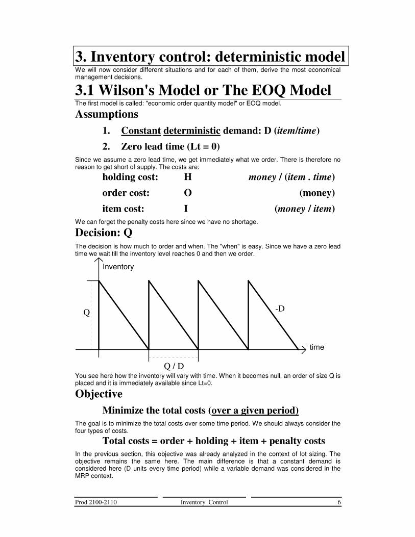
Decision: Q The decision is how much to order and when. The "when" is easy. Since we have a zero lead time we wait till the inventory level reaches 0 and then we order.

Q

Q / D

time

Inventory

-D

You see here how the inventory will vary with time. When it becomes null, an order of size Q is placed and it is immediately available since Lt=0.

Objective Minimize the total costs (over a given period)

The goal is to minimize the total costs over some time period. We should always consider the four types of costs.

Total costs = order + holding + item + penalty costs In the previous section, this objective was already analyzed in the context of lot sizing. The objective remains the same here. The main difference is that a constant demand is considered here (D units every time period) while a variable demand was considered in the MRP context.


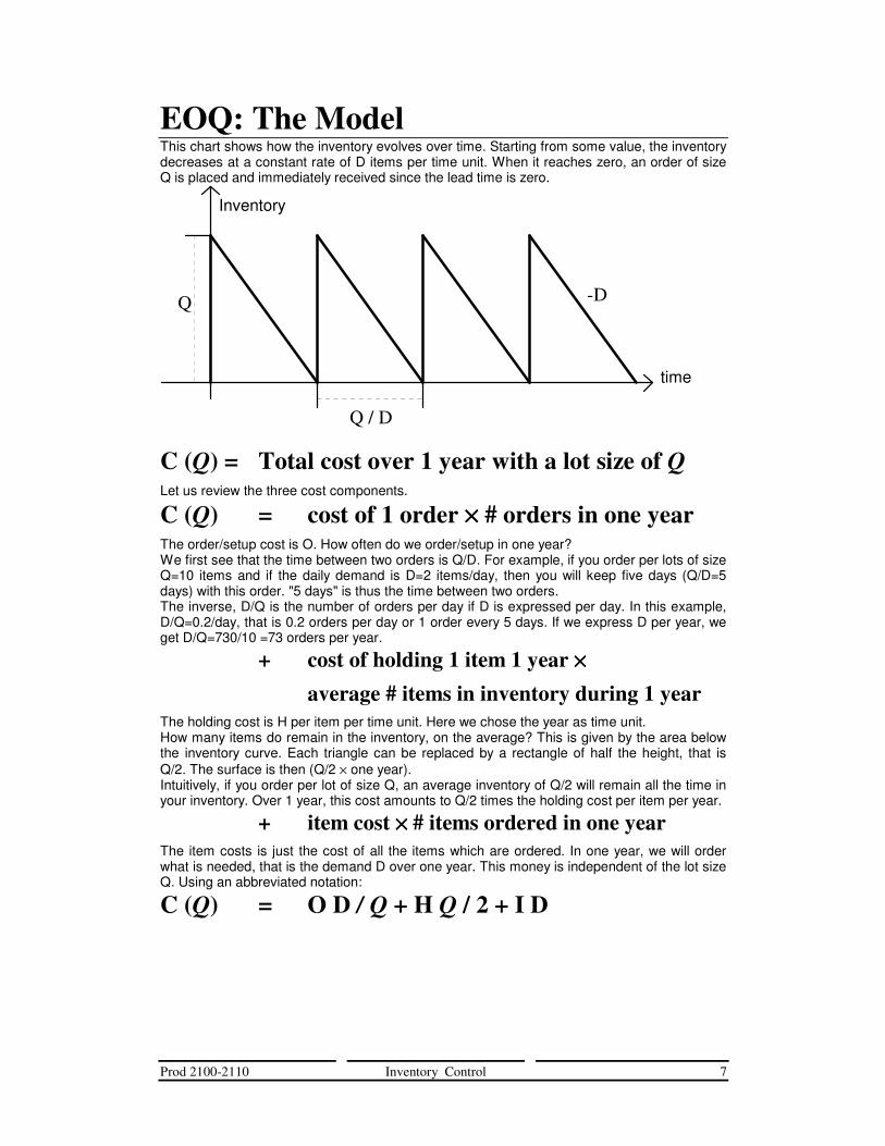
EOQ: The Model This chart shows how the inventory evolves over time. Starting from some value, the inventory decreases at a constant rate of D items per time unit. When it reaches zero, an order of size Q is placed and immediately received since the lead time is zero.

Q

Q / D

time

Inventory

-D

C (Q) = Total cost over 1 year with a lot size of Q Let us review the three cost components.

C (Q) = cost of 1 order ×××× # orders in one year The order/setup cost is O. How often do we order/setup in one year? We first see that the time between two orders is Q/D. For example, if you order per lots of size Q=10 items and if the daily demand is D=2 items/day, then you will keep five days (Q/D=5 days) with this order. "5 days" is thus the time between two orders. The inverse, D/Q is the number of orders per day if D is expressed per day. In this example, D/Q=0.2/day, that is 0.2 orders per day or 1 order every 5 days. If we express D per year, we get D/Q=730/10 =73 orders per year.

+ cost of holding 1 item 1 year ×××× average # items in inventory during 1 year

The holding cost is H per item per time unit. Here we chose the year as time unit. How many items do remain in the inventory, on the average? This is given by the area below the inventory curve. Each triangle can be replaced by a rectangle of half the height, that is Q/2. The surface is then (Q/2 × one year). Intuitively, if you order per lot of size Q, an average inventory of Q/2 will remain all the time in your inventory. Over 1 year, this cost amounts to Q/2 times the holding cost per item per year.

+ item cost ×××× # items ordered in one year The item costs is just the cost of all the items which are ordered. In one year, we will order what is needed, that is the demand D over one year. This money is independent of the lot size Q. Using an abbreviated notation:

C (Q) = O D / Q + H Q / 2 + I D


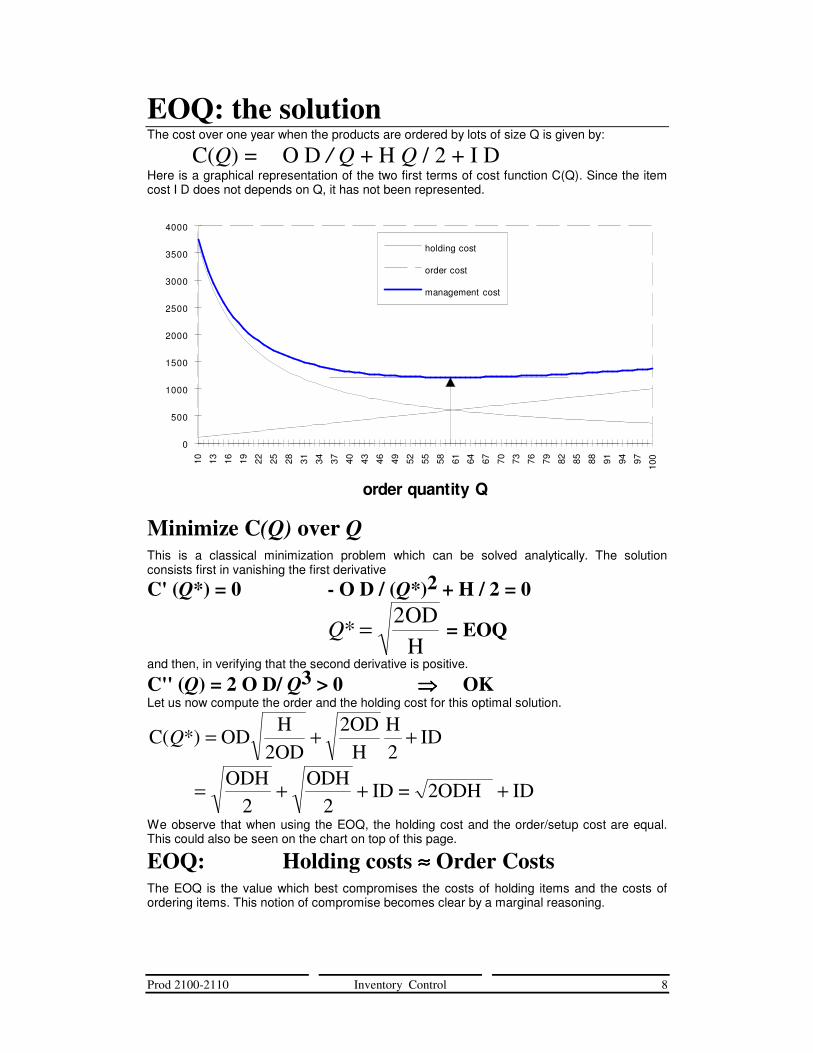
EOQ: the solution The cost over one year when the products are ordered by lots of size Q is given by:

C(Q) = O D / Q + H Q / 2 + I D Here is a graphical representation of the two first terms of cost function C(Q). Since the item cost I D does not depends on Q, it has not been represented.

order quantity Q

0

500

1000

1500

2000

2500

3000

3500

4000

10 13 16 19 22 25 28 31 34 37 40 43 46 49 52 55 58 61 64 67 70 73 76 79 82 85 88 91 94 97

100

holding cost

order cost

management cost

Minimize C(Q) over Q This is a classical minimization problem which can be solved analytically. The solution consists first in vanishing the first derivative

C' (Q*) = 0 - O D / (Q*)2 + H / 2 = 0

Q* = 2ODH

= EOQ and then, in verifying that the second derivative is positive.

C'' (Q) = 2 O D/ Q3 > 0 �� OK Let us now compute the order and the holding cost for this optimal solution.

C ODH

2OD2OD

HH2

ID( *)Q = + +

= + + +ODH2

ODH2

ID = 2ODH ID We observe that when using the EOQ, the holding cost and the order/setup cost are equal. This could also be seen on the chart on top of this page.

EOQ: Holding costs ≈≈≈≈ Order Costs The EOQ is the value which best compromises the costs of holding items and the costs of ordering items. This notion of compromise becomes clear by a marginal reasoning.


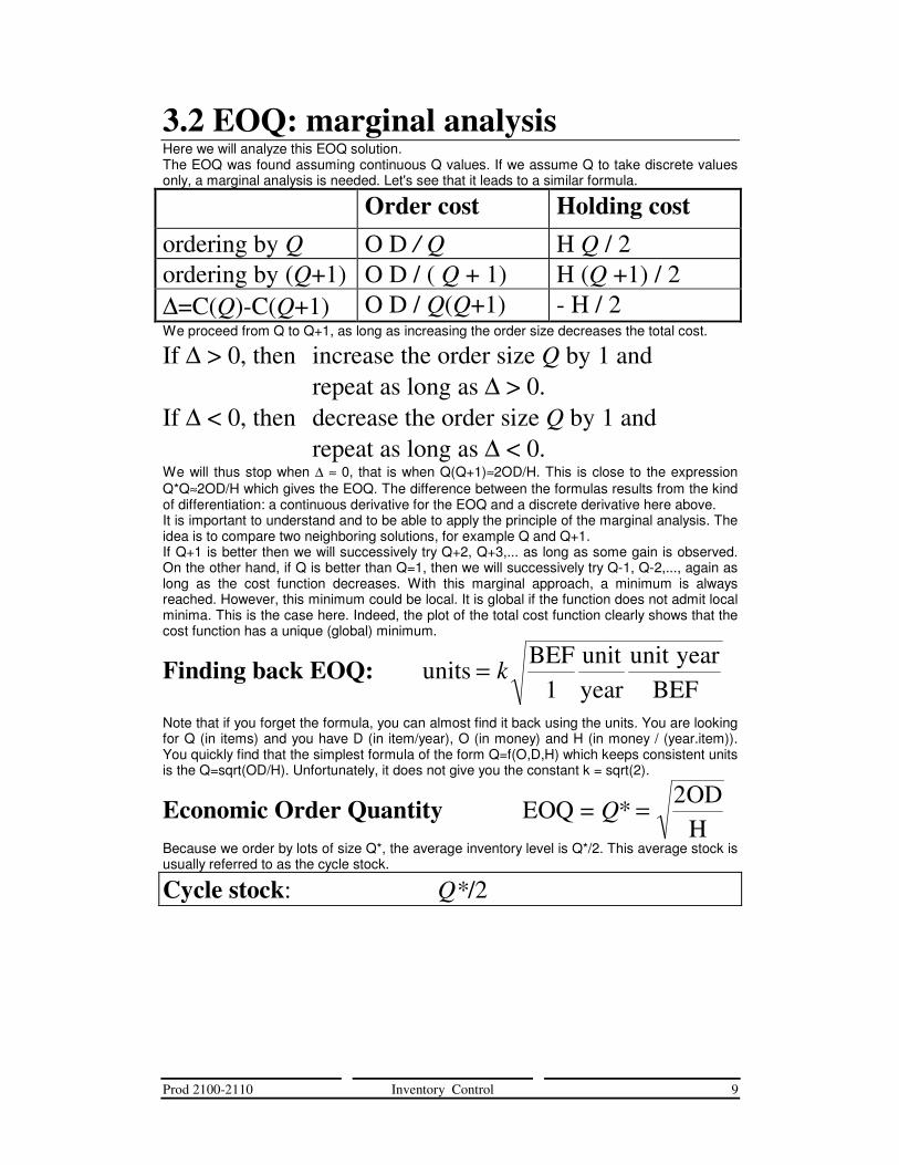
3.2 EOQ: marginal analysis Here we will analyze this EOQ solution. The EOQ was found assuming continuous Q values. If we assume Q to take discrete values only, a marginal analysis is needed. Let's see that it leads to a similar formula.

Order cost Holding cost ordering by Q O D / Q H Q / 2 ordering by (Q+1) O D / ( Q + 1) H (Q +1) / 2 ∆=C(Q)-C(Q+1) O D / Q(Q+1) - H / 2 We proceed from Q to Q+1, as long as increasing the order size decreases the total cost.

If ∆ > 0, then increase the order size Q by 1 and repeat as long as ∆ > 0.

If ∆ < 0, then decrease the order size Q by 1 and repeat as long as ∆ < 0.

We will thus stop when ∆ ≈ 0, that is when Q(Q+1)≈2OD/H. This is close to the expression Q*Q≈2OD/H which gives the EOQ. The difference between the formulas results from the kind of differentiation: a continuous derivative for the EOQ and a discrete derivative here above. It is important to understand and to be able to apply the principle of the marginal analysis. The idea is to compare two neighboring solutions, for example Q and Q+1. If Q+1 is better then we will successively try Q+2, Q+3,... as long as some gain is observed. On the other hand, if Q is better than Q=1, then we will successively try Q-1, Q-2,..., again as long as the cost function decreases. With this marginal approach, a minimum is always reached. However, this minimum could be local. It is global if the function does not admit local minima. This is the case here. Indeed, the plot of the total cost function clearly shows that the cost function has a unique (global) minimum.

Finding back EOQ: unitsBEF

1unityear

unit yearBEF

= k

Note that if you forget the formula, you can almost find it back using the units. You are looking for Q (in items) and you have D (in item/year), O (in money) and H (in money / (year.item)). You quickly find that the simplest formula of the form Q=f(O,D,H) which keeps consistent units is the Q=sqrt(OD/H). Unfortunately, it does not give you the constant k = sqrt(2).

Economic Order Quantity EOQ = Q* = 2ODH

Because we order by lots of size Q*, the average inventory level is Q*/2. This average stock is usually referred to as the cycle stock.

Cycle stock: Q*/2


3.3 EOQ: examples and sensitivity

Economic Order Quantity EOQ = Q* = 2ODH

Examples D (box/y.)

O (BEF)

H (BEF/box/y)

Q* (box)

M(Q*) (BEF)

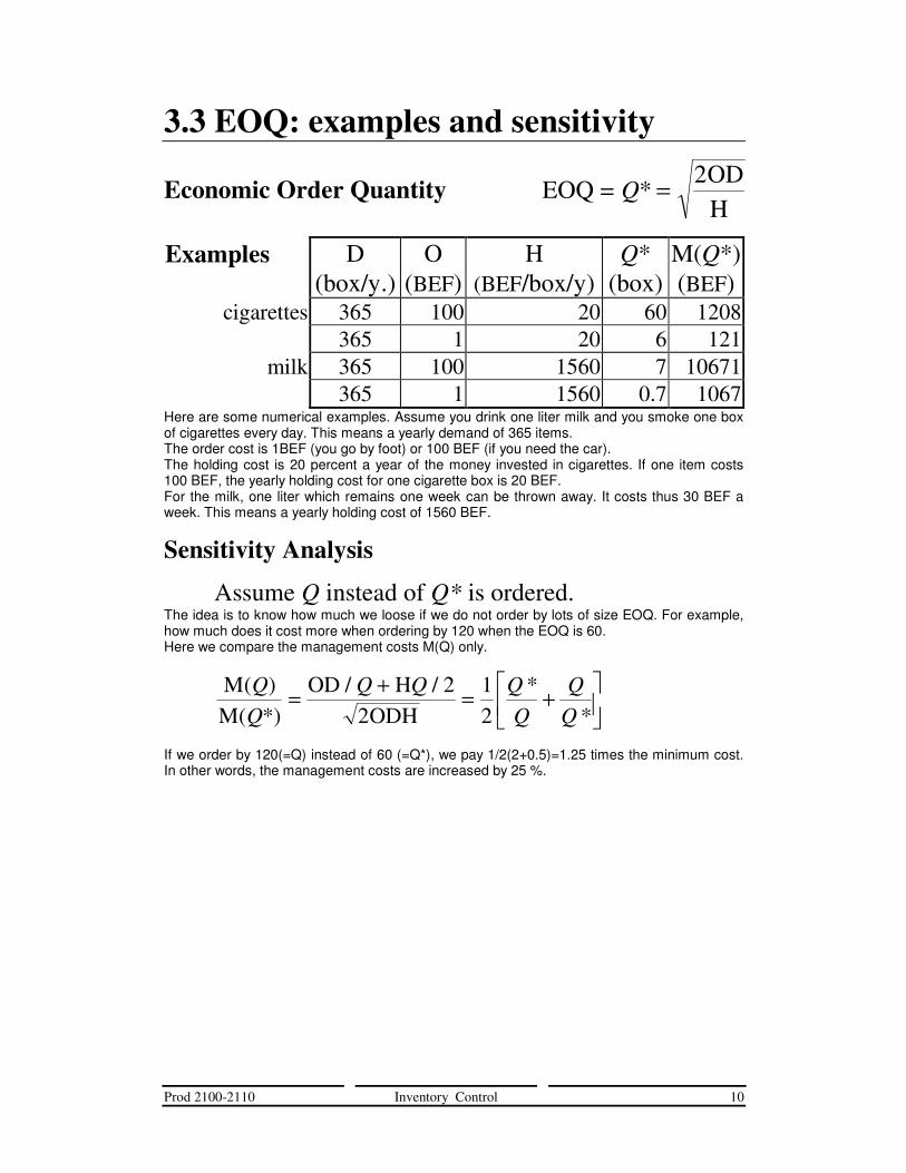
cigarettes 365 100 20 60 1208 365 1 20 6 121

milk 365 100 1560 7 10671 365 1 1560 0.7 1067 Here are some numerical examples. Assume you drink one liter milk and you smoke one box of cigarettes every day. This means a yearly demand of 365 items. The order cost is 1BEF (you go by foot) or 100 BEF (if you need the car). The holding cost is 20 percent a year of the money invested in cigarettes. If one item costs 100 BEF, the yearly holding cost for one cigarette box is 20 BEF. For the milk, one liter which remains one week can be thrown away. It costs thus 30 BEF a week. This means a yearly holding cost of 1560 BEF.

Sensitivity Analysis

Assume Q instead of Q* is ordered. The idea is to know how much we loose if we do not order by lots of size EOQ. For example, how much does it cost more when ordering by 120 when the EOQ is 60. Here we compare the management costs M(Q) only.

MM

OD HODH

( )( *)

/ / **

QQ

Q Q QQ

QQ

= + = +�

��

�

��

22

12

If we order by 120(=Q) instead of 60 (=Q*), we pay 1/2(2+0.5)=1.25 times the minimum cost. In other words, the management costs are increased by 25 %.


3.4 EOQ with positive Lead time. Let us consider again the EOQ model but let us assume that the time between an order is placed and the same order is received is nonnull.

Assumptions: 1. Constant deterministic demand: D (item / time ) 2. Positive lead time (Lt > 0)

We will see that the costs do not change. Shortages are still avoided. Since the costs do not change, we will still order by Q* but we will order earlier.

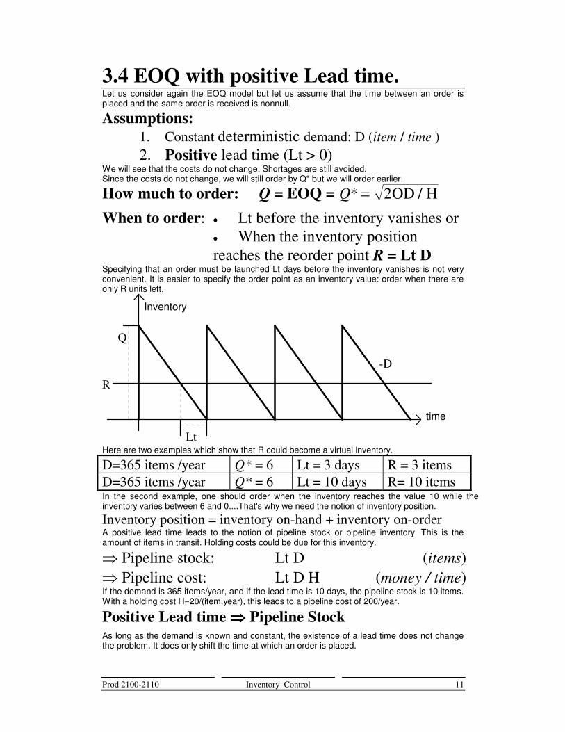
How much to order: Q = EOQ = Q* = 2OD / H When to order: •••• Lt before the inventory vanishes or

•••• When the inventory position reaches the reorder point R = Lt D

Specifying that an order must be launched Lt days before the inventory vanishes is not very convenient. It is easier to specify the order point as an inventory value: order when there are only R units left.

Q

Lt

time

Inventory

-D

R

Here are two examples which show that R could become a virtual inventory.

D=365 items /year Q* = 6 Lt = 3 days R = 3 items D=365 items /year Q* = 6 Lt = 10 days R= 10 items In the second example, one should order when the inventory reaches the value 10 while the inventory varies between 6 and 0....That's why we need the notion of inventory position.

Inventory position = inventory on-hand + inventory on-order A positive lead time leads to the notion of pipeline stock or pipeline inventory. This is the amount of items in transit. Holding costs could be due for this inventory.

� Pipeline stock: Lt D (items) � Pipeline cost: Lt D H (money / time) If the demand is 365 items/year, and if the lead time is 10 days, the pipeline stock is 10 items. With a holding cost H=20/(item.year), this leads to a pipeline cost of 200/year.

Positive Lead time �� Pipeline Stock As long as the demand is known and constant, the existence of a lead time does not change the problem. It does only shift the time at which an order is placed.


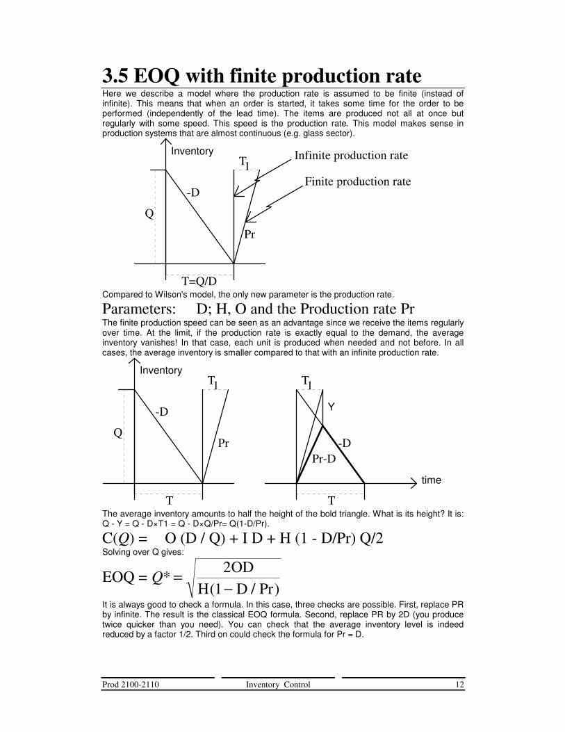
3.5 EOQ with finite production rate Here we describe a model where the production rate is assumed to be finite (instead of infinite). This means that when an order is started, it takes some time for the order to be performed (independently of the lead time). The items are produced not all at once but regularly with some speed. This speed is the production rate. This model makes sense in production systems that are almost continuous (e.g. glass sector).

InventoryT1

Q

T=Q/D

Pr

-D

Infinite production rate

Finite production rate

Compared to Wilson's model, the only new parameter is the production rate.

Parameters: D; H, O and the Production rate Pr The finite production speed can be seen as an advantage since we receive the items regularly over time. At the limit, if the production rate is exactly equal to the demand, the average inventory vanishes! In that case, each unit is produced when needed and not before. In all cases, the average inventory is smaller compared to that with an infinite production rate.

time

InventoryT1

Q

T

Pr

-D

T

T1

Pr-D-D

Y

The average inventory amounts to half the height of the bold triangle. What is its height? It is: Q - Y = Q - D×T1 = Q - D×Q/Pr= Q(1-D/Pr).

C(Q) = O (D / Q) + I D + H (1 - D/Pr) Q/2 Solving over Q gives:

EOQ = Q* =−2OD

H(1 D / Pr)

It is always good to check a formula. In this case, three checks are possible. First, replace PR by infinite. The result is the classical EOQ formula. Second, replace PR by 2D (you produce twice quicker than you need). You can check that the average inventory level is indeed reduced by a factor 1/2. Third on could check the formula for Pr = D.


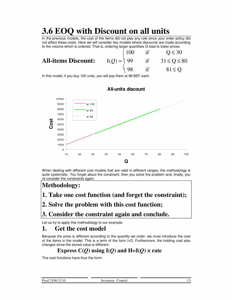
3.6 EOQ with Discount on all units In the previous models, the cost of the items did not play any role since your order policy did not affect these costs. Here we will consider two models where discounts are made according to the volume which is ordered. That is, ordering larger quantities Q lead to lower prices.

All-items Discount: Iif Q 30if 31 Q 80if Q

( )Q =≤

≤ ≤≤

�

��

1009998 81

In this model, if you buy 100 units, you will pay them at 98 BEF each.

All-units discount

Q

Cos

t

0

1000

2000

3000

4000

5000

6000

7000

8000

9000

10000

10 20 30 40 50 60 70 80 90 100

at 100

at 99

at 98

When dealing with different cost models that are valid in different ranges, the methodology is quite systematic. You forget about the constraint, then you solve the problem and, finally, you re-consider the constraints again.

Methodology: 1. Take one cost function (and forget the constraint); 2. Solve the problem with this cost function; 3. Consider the constraint again and conclude. Let us try to apply this methodology to our example.

1. Get the cost model Because the price is different according to the quantity we order, we must introduce the cost of the items in the model. This is a term of the form I×D. Furthermore, the holding cost also changes since the stored value is different.

Express C(Q) using I(Q) and H=I(Q) ×××× rate The cost functions have thus the form:


C ( ) OD / 100 D H / 2

C ( ) OD / 99 D H / 2

C ( ) OD / 98 D H / 2

100 100

99 99

98 98

Q Q Q

Q Q Q

Q Q Q

= + +

= + +

= + +

��

��

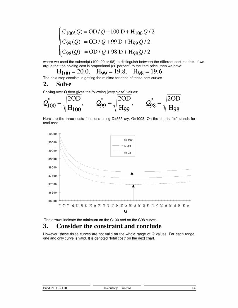
where we used the subscript (100, 99 or 98) to distinguish between the different cost models. If we argue that the holding cost is proportional (20 percent) to the item price, then we have:

H , H , H100 99 9820 0 19 8 19 6= = =. . . The next step consists in getting the minima for each of these cost curves.

2. Solve Solving over Q then gives the following (very close) values:

Q Q Q100 99 98* * *,= = =2OD

H2ODH

,2ODH100 99 98

Here are the three costs functions using D=365 u/y, O=100$. On the charts, “tc” stands for total cost.

Q

36000

36500

37000

37500

38000

38500

39000

39500

40000

11 14 17 20 23 26 29 32 35 38 41 44 47 50 53 56 59 62 65 68 71 74 77 80 83 86 89 92 95 98

tc-100

tc-99

tc-98

The arrows indicate the minimum on the C100 and on the C98 curves.

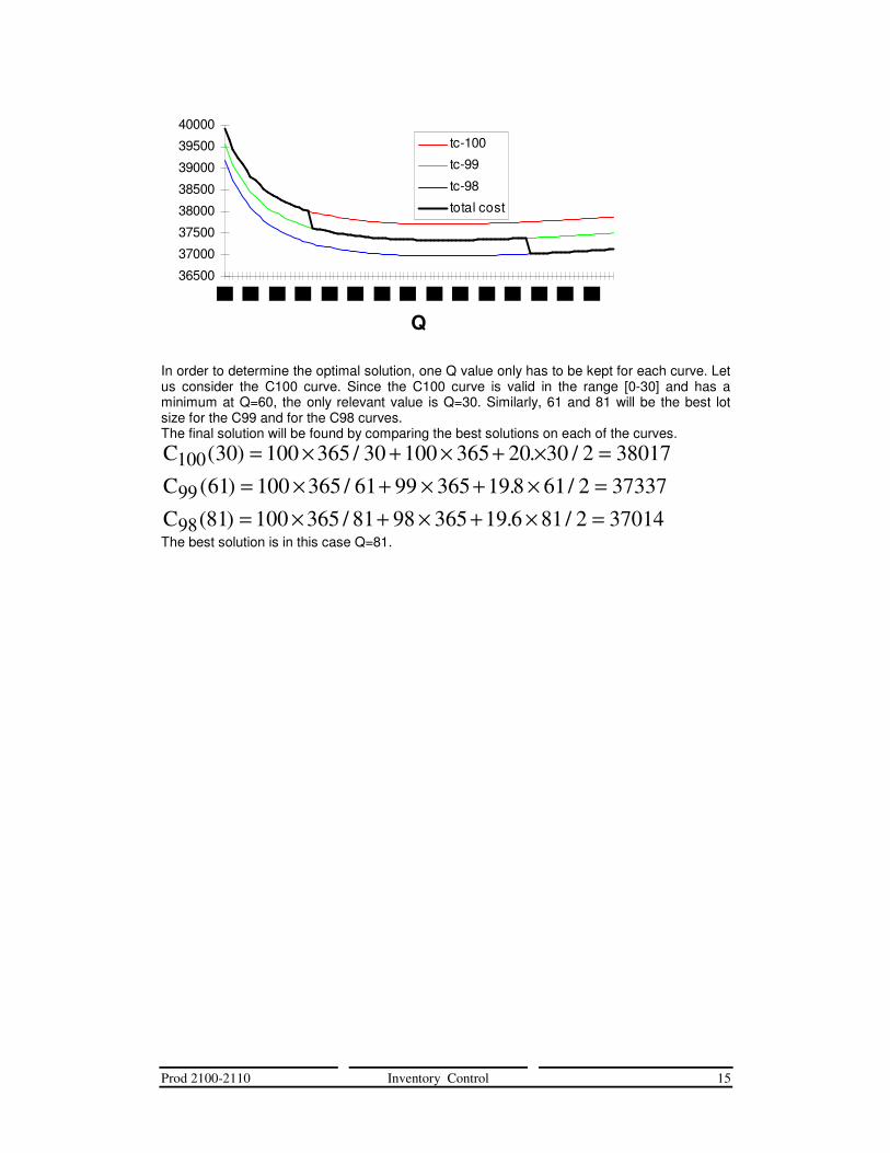
3. Consider the constraint and conclude However, these three curves are not valid on the whole range of Q values. For each range, one and only curve is valid. It is denoted "total cost" on the next chart.


36500

37000

37500

38000

38500

39000

39500

40000

Q

tc-100

tc-99

tc-98

total cost

In order to determine the optimal solution, one Q value only has to be kept for each curve. Let us consider the C100 curve. Since the C100 curve is valid in the range [0-30] and has a minimum at Q=60, the only relevant value is Q=30. Similarly, 61 and 81 will be the best lot size for the C99 and for the C98 curves. The final solution will be found by comparing the best solutions on each of the curves.

CCC

100

99

98

30 100 365 30 100 365 20 30 2 3801761 100 365 61 99 365 19 8 61 2 3733781 100 365 81 98 365 19 6 81 2 37014

( ) / . /( ) / . /( ) / . /

= × + × + × == × + × + × == × + × + × =

The best solution is in this case Q=81.


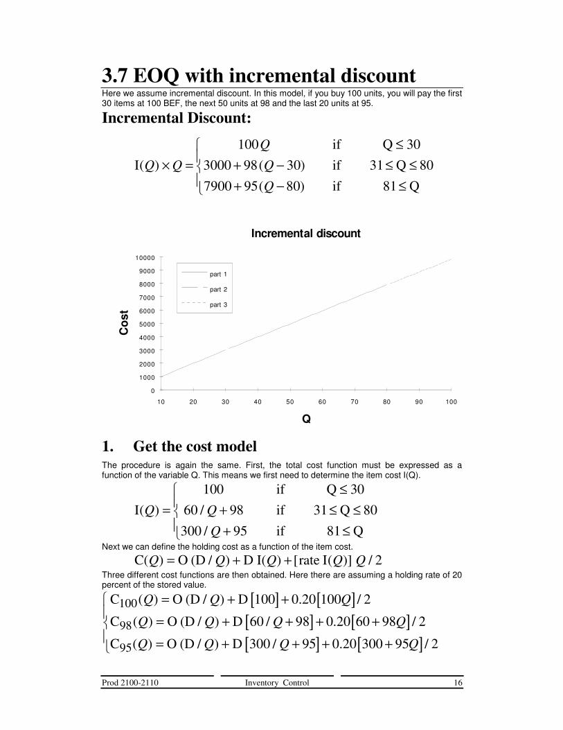
3.7 EOQ with incremental discount Here we assume incremental discount. In this model, if you buy 100 units, you will pay the first 30 items at 100 BEF, the next 50 units at 98 and the last 20 units at 95.

Incremental Discount:

Iif Q 30if 31 Q 80if Q

( ) ( )( )

Q Q

Q

Q

Q

× =≤

+ − ≤ ≤+ − ≤

�

��

1003000 98 307900 95 80 81

Incremental discount

Q

Cos

t

0

1000

2000

3000

4000

5000

6000

7000

8000

9000

10000

10 20 30 40 50 60 70 80 90 100

part 1

part 2

part 3

1. Get the cost model The procedure is again the same. First, the total cost function must be expressed as a function of the variable Q. This means we first need to determine the item cost I(Q).

Iif Q 30if 31 Q 80if Q

( ) //

Q Q

Q

=≤

+ ≤ ≤+ ≤

�

��

10060 98300 95 81

Next we can define the holding cost as a function of the item cost.

C( ) O (D / ) D I( ) rate I / 2Q Q Q Q Q= + + [ ( )] Three different cost functions are then obtained. Here there are assuming a holding rate of 20 percent of the stored value.

[ ] [ ][ ] [ ][ ] [ ]

C ( ) O (D / ) D 100 0.20 100 / 2

C ( ) O (D / ) D 98 0.20 60 98 / 2

C ( ) O (D / ) D 95 0.20 300 95 / 2

100

98

95

Q Q Q

Q Q Q Q

Q Q Q Q

= + += + + + += + + + +

�

��

60

300

/

/


Compared to the C100 curve, it seems that the order cost (the coefficient of D/Q) has been increased in the C98 curve by a fixed amount 60. These 60 correspond to the extra cost we have to pay for the first 30 units. Indeed, in the C98 expression, each unit is paid 98 and we have to add an extra fixed cost of 2 for each of the 30 first units. A similar comment applies to the curve C95.

Incremental discount

36000

38000

40000

42000

44000

46000

48000

11 14 17 20 23 26 29 32 35 38 41 44 47 50 53 56 59 62 65 68 71 74 77 80 83 86 89 92 95 98

tc-100

tc-98

tc-95

Here are the three curves. Again, there are only valid on a part of the range of Q values.

2. Solve Assuming D=365 items/year and O=100Bef, we obtain the following optimal values.

Q

Q

Q

100

98

95

2 100 365 20 60

2 100 60 365 19 6 77

2 100 300 365 19 0 124

*

*

*

( )( ) /

( )( ) / .

( )( ) / .

= ≈

= + ≈

= + ≈

��

��

3. Consider the constraints and conclude Again, for each cost curve, only one value must be considered. These three values are 30, 77 and 124, respectively. Computing the corresponding costs lead to the values:

[ ] [ ]C

C C

100

98 95

30 10036530

365 100 01 100 30 38017

77 37289 124 37060

( ) .

( ) ; ( )

= + + × ≈

≈ ≈

�

��

The optimal solution consists thus in ordering by lots of size 124.


3.8 Economic Replenishment Interval Up to now, we always considered that the lot size Q was the variable. We could also have chosen T, the interval between two orders. Since Q and T are related by the formula: T D = Q, this leads to the following cost formulation.

C(T) = O / T + I D + H T D /2 Solving in T leads to the optimal replenishment interval T*.

Economic Replenishment Interval: T* = 2OHD

Economic Order Quantity Q* = 2ODH

Computing the optimal replenishment interval is more adequate when several different items have to be ordered with a same order cost. A first typical situation is when you order several products from a same supplier. Your administration costs are usually independent of the mix and of the quantities which are ordered. The transport cost (which could be the dominant part of the order cost) may also be fixed. A machine whose setup is valid for a family of products can also be seen as a fixed unique cost for different products.

Method for computing an optimal policy: 1. express all the costs in terms of Q or T (you might have different curves); 2. determine the minimum on each curve; 3. check whether the minimum is feasible and modify it if necessary; 4. choose the best solution;


4 Inventory control: Stochastic Models Up to now we considered models with deterministic and constant demand. We will now address problems where the demand is subject to stochastic variations.

4.1 Random Demand The EOQ models look for a compromise between the holding, the order and item costs.

Deterministic Demand: Holding cost

↔ Order Cost Item Cost

Q

Lttime

Inventory

-D

R

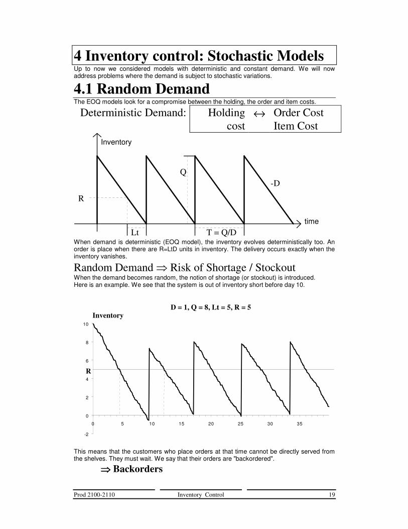
T = Q/D When demand is deterministic (EOQ model), the inventory evolves deterministically too. An order is place when there are R=LtD units in inventory. The delivery occurs exactly when the inventory vanishes.

Random Demand � Risk of Shortage / Stockout When the demand becomes random, the notion of shortage (or stockout) is introduced. Here is an example. We see that the system is out of inventory short before day 10.

D = 1, Q = 8, Lt = 5, R = 5

-2

0

2

4

6

8

10

0 5 10 15 20 25 30 35

Inventory

R

This means that the customers who place orders at that time cannot be directly served from the shelves. They must wait. We say that their orders are "backordered".

�� Backorders


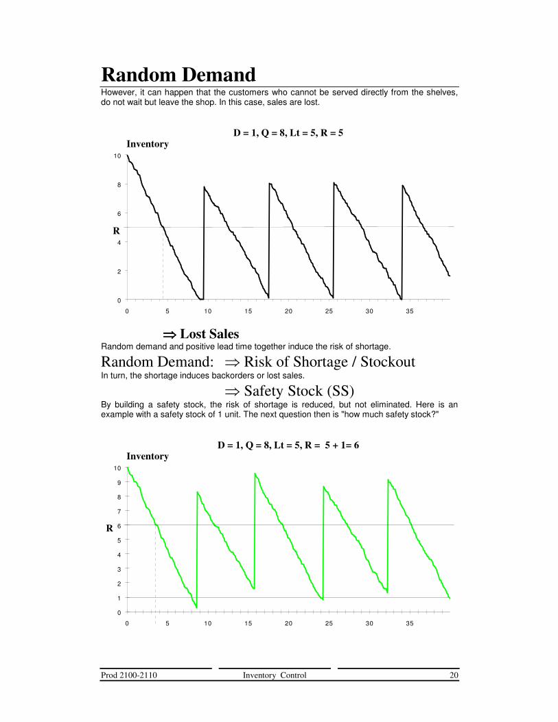
Random Demand However, it can happen that the customers who cannot be served directly from the shelves, do not wait but leave the shop. In this case, sales are lost.

D = 1, Q = 8, Lt = 5, R = 5

0

2

4

6

8

10

0 5 10 15 20 25 30 35

Inventory

R

�� Lost Sales Random demand and positive lead time together induce the risk of shortage.

Random Demand: � Risk of Shortage / Stockout In turn, the shortage induces backorders or lost sales.

� Safety Stock (SS) By building a safety stock, the risk of shortage is reduced, but not eliminated. Here is an example with a safety stock of 1 unit. The next question then is "how much safety stock?"

D = 1, Q = 8, Lt = 5, R = 5 + 1= 6

0

1

2

3

4

5

6

7

8

9

10

0 5 10 15 20 25 30 35

Inventory

R


4.2 Lot size - reorder point model or (Q, R) model Let us try here to summarize the problem. The assumptions are the following.

Assumptions 1. Constant random demand: D (item / time ) 2. Lead time (Lt> 0) 3. Continuous review

Four different cost areas have to be considered. Here are the associated parameters.

Costs: Holding, Order, Item, Penalty Random demand and positive lead time together induce the risk of shortage and therefore of possible penalty costs.

Decision (lot size - reorder point) Select Q and R = Lt × D + SS

The decision variables are the order lot size Q and the order point R. Since R is basically defined as the demand during the lead time plus the safety stock, choosing R is equivalent to choosing the safety stock SS.

General Objective Minimize the costs / Optimize the service

These are the two general goals which are pursued. The notion of "good service" requires however further specifications. Here are two classical ways.

Objective 1 Minimize the total costs and Guarantee a maximum stockout frequency (f)

This means that the safety stock will be chosen in order to guarantee that the frequency of stocking out does not exceed some given value (e.g., once a year).

Objective 2 Minimize the total costs and Guarantee a minimum fill rate (ββββ)

The fill rate(β) is the average percentage of the sales which are directly satisfied from the shelves. The goal here is thus to select the safety stock which guarantee that, for example, 95 percent of the units ordered can be immediately served from the stock.

Objective 3 Minimize the total costs (assuming penalty costs)

Here we assume that each demand unit that is backordered induces a penalty cost (which is independent of the time the unit is backordered). Knowing this cost, we can choose the best safety stock SS and the best lost size Q by a pure economical analysis.


Demand during the Lead Time: DLt Whichever objective is selected, we need to know the distribution of the demand during the lead time in order to be able to compute the required figures.

Objective 1 � compute the stockout frequency f � compute the cycle stockout probability α � Prob[ DLt > R] In order to compute this stockout probability, the distribution of D(Lt) must be known.

Objective 2 � Compute the fill rate β � Compute the average number of units during a

cycle which are not served from the shelves: n(R) � n(R) = 1 × Prob[ DLt = R+1] + 2 × Prob[ DLt = R+2] + 3 × Prob[ DLt = R+3] + ...

To determine the fill rate, we must determine who is served from the shelve and who is not. We therefore need to know the average number of backlogged orders n(R). Therefore, the distribution of the demand during the lead time is needed.

Objective 3 � Compute the penalty costs

� Compute n(R) � Prob[ DLt = R+1, ...] With any of the three different objectives considered, the demand during the lead time must be known. To know this demand means to know its complete probability distribution. In many cases however, we just know the mean and the standard deviation and we have to make some assumption about the shape of its probability distribution.

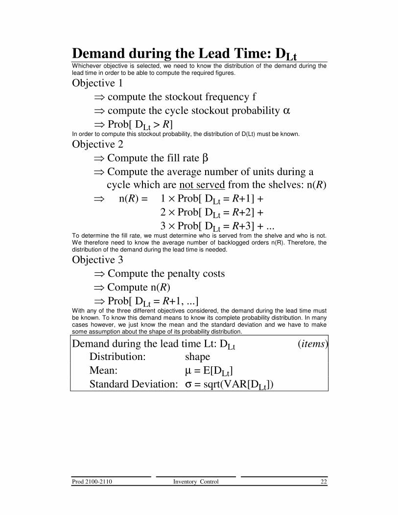
Demand during the lead time Lt: DLt (items) Distribution: shape Mean: µ = E[DLt] Standard Deviation: σ = sqrt(VAR[DLt])


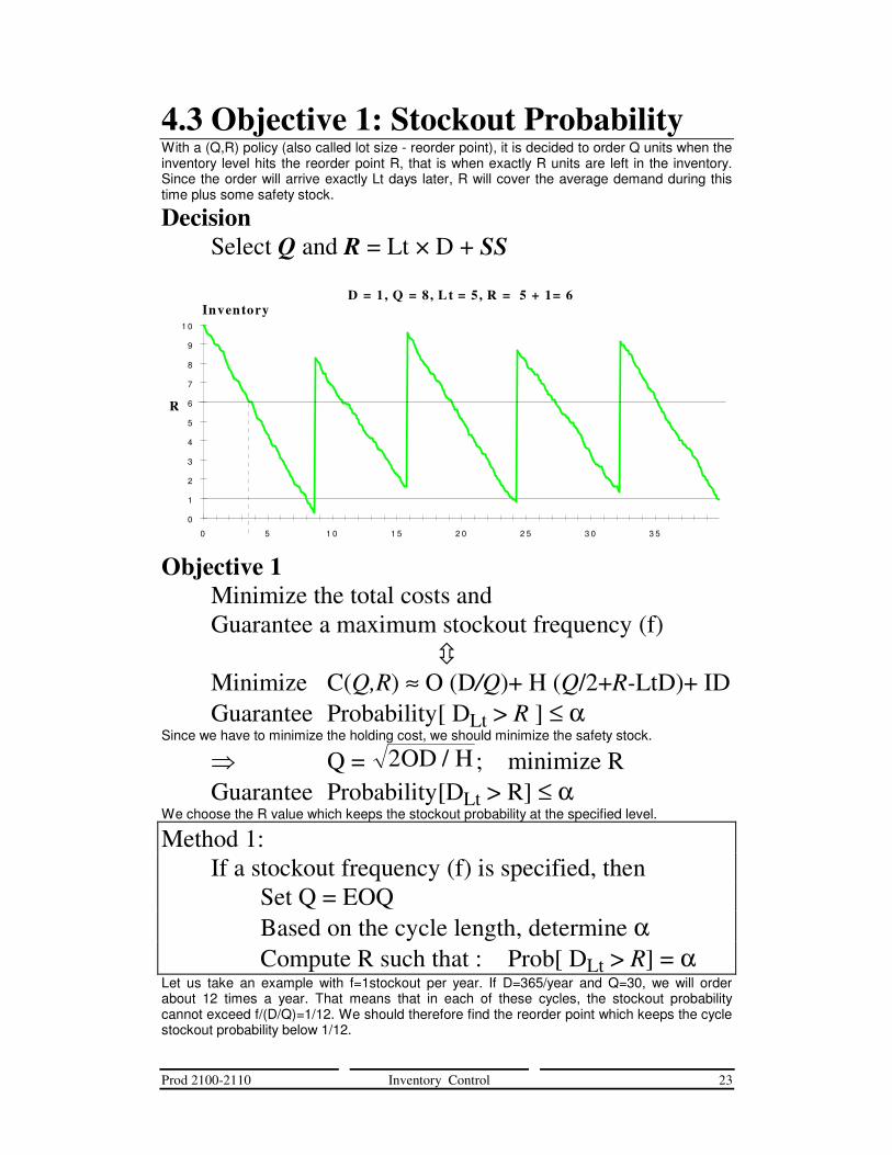
4.3 Objective 1: Stockout Probability With a (Q,R) policy (also called lot size - reorder point), it is decided to order Q units when the inventory level hits the reorder point R, that is when exactly R units are left in the inventory. Since the order will arrive exactly Lt days later, R will cover the average demand during this time plus some safety stock.

Decision Select Q and R = Lt × D + SS

D = 1, Q = 8, L t = 5, R = 5 + 1= 6

0

1

2

3

4

5

6

7

8

9

1 0

0 5 1 0 1 5 2 0 2 5 3 0 3 5

Inventory

R

Objective 1 Minimize the total costs and Guarantee a maximum stockout frequency (f)

� Minimize C(Q,R) ≈ O (D/Q)+ H (Q/2+R-LtD)+ ID Guarantee Probability[ DLt > R ] ≤ α

Since we have to minimize the holding cost, we should minimize the safety stock.

� Q = 2OD / H ; minimize R Guarantee Probability[DLt > R] ≤ α

We choose the R value which keeps the stockout probability at the specified level.

Method 1: If a stockout frequency (f) is specified, then Set Q = EOQ Based on the cycle length, determine α Compute R such that : Prob[ DLt > R] = α Let us take an example with f=1stockout per year. If D=365/year and Q=30, we will order about 12 times a year. That means that in each of these cycles, the stockout probability cannot exceed f/(D/Q)=1/12. We should therefore find the reorder point which keeps the cycle stockout probability below 1/12.


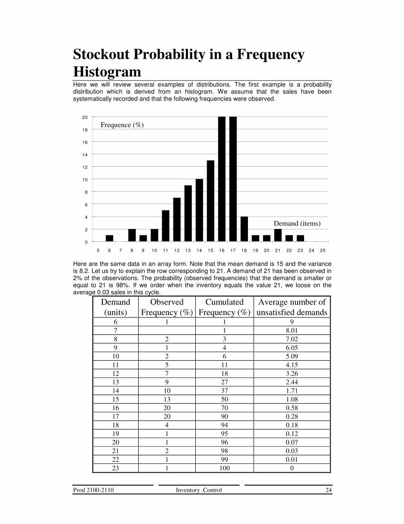
Stockout Probability in a Frequency Histogram Here we will review several examples of distributions. The first example is a probability distribution which is derived from an histogram. We assume that the sales have been systematically recorded and that the following frequencies were observed.

0

2

4

6

8

10

12

14

16

18

20

5 6 7 8 9 10 11 12 13 14 15 16 17 18 19 20 21 22 23 24 25

Frequence (%)

Demand (items)

Here are the same data in an array form. Note that the mean demand is 15 and the variance is 8.2. Let us try to explain the row corresponding to 21. A demand of 21 has been observed in 2% of the observations. The probability (observed frequencies) that the demand is smaller or equal to 21 is 98%. If we order when the inventory equals the value 21, we loose on the average 0.03 sales in this cycle.

Demand (units)

Observed Frequency (%)

Cumulated Frequency (%)

Average number of unsatisfied demands

6 1 1 9 7 1 8.01 8 2 3 7.02 9 1 4 6.05

10 2 6 5.09 11 5 11 4.15 12 7 18 3.26 13 9 27 2.44 14 10 37 1.71 15 13 50 1.08 16 20 70 0.58 17 20 90 0.28 18 4 94 0.18 19 1 95 0.12 20 1 96 0.07 21 2 98 0.03 22 1 99 0.01 23 1 100 0


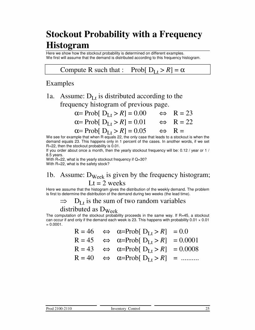
Stockout Probability with a Frequency Histogram Here we show how the stockout probability is determined on different examples. We first will assume that the demand is distributed according to this frequency histogram.

Compute R such that : Prob[ DLt > R] = α

Examples

1a. Assume: DLt is distributed according to the frequency histogram of previous page. α= Prob[ DLt > R] = 0.00 ⇔ R = 23 α= Prob[ DLt > R] = 0.01 ⇔ R = 22 α= Prob[ DLt > R] = 0.05 ⇔ R =

We see for example that when R equals 22, the only case that leads to a stockout is when the demand equals 23. This happens only in 1 percent of the cases. In another words, if we set R=22, then the stockout probability is 0.01. If you order about once a month, then the yearly stockout frequency will be: 0.12 / year or 1 / 8.5 years. With R=22, what is the yearly stockout frequency if Q=30? With R=22, what is the safety stock?

1b. Assume: DWeek is given by the frequency histogram; Lt = 2 weeks Here we assume that the histogram gives the distribution of the weekly demand. The problem is first to determine the distribution of the demand during two weeks (the lead time).

� DLt is the sum of two random variables distributed as DWeek

The computation of the stockout probability proceeds in the same way. If R=45, a stockout can occur if and only if the demand each week is 23. This happens with probability 0.01 × 0.01 = 0.0001.

R = 46 ⇔ α=Prob[ DLt > R] = 0.0 R = 45 ⇔ α=Prob[ DLt > R] = 0.0001 R = 43 ⇔ α=Prob[ DLt > R] = 0.0008 R = 40 ⇔ α=Prob[ DLt > R] = ..........


Stockout Probability with a Continuous Uniform Distribution Let us now consider two continuous distributions: the uniform and the normal distributions.


0

0.005

0.01

-20 0

20 40 60 80

100

120

140

160

180

200

220

uniform

1.75 σ

Note that in the uniform distribution, the standard deviation is about (max - min)/3.5. In this example, the mean is thus 100 and the standard deviation, about 30.

2. Assume: DLt is continuous and uniform [50-150]

α = 0.00 ⇔ R = 150 SS = ...... α = 0.01 ⇔ R = 149 SS = ...... α = 0.05 ⇔ R = 145 SS = ...... α = 0.10 ⇔ R = ...... SS = ......


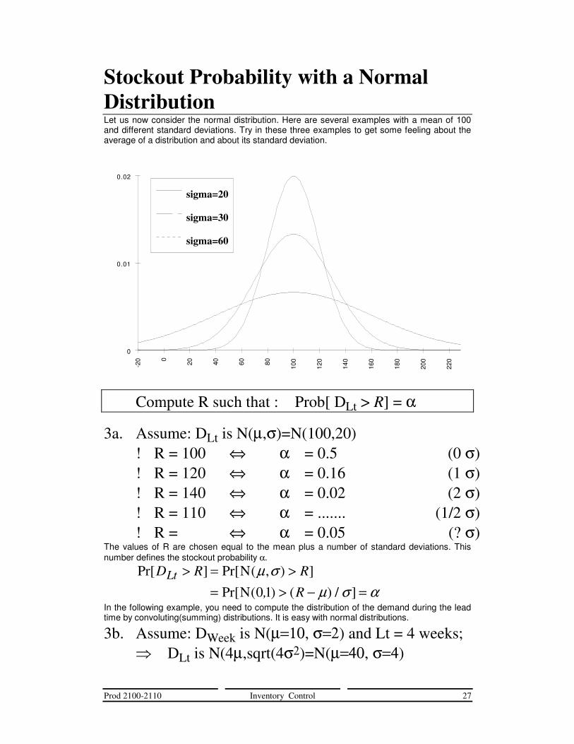
Stockout Probability with a Normal Distribution Let us now consider the normal distribution. Here are several examples with a mean of 100 and different standard deviations. Try in these three examples to get some feeling about the average of a distribution and about its standard deviation.

0

0.01

0.02

-20 0

20 40 60 80

100

120

140

160

180

200

220

sigma=20

sigma=30

sigma=60


3a. Assume: DLt is N(µ,σ)=N(100,20) ! R = 100 ⇔ α = 0.5 (0 σ) ! R = 120 ⇔ α = 0.16 (1 σ) ! R = 140 ⇔ α = 0.02 (2 σ) ! R = 110 ⇔ α = ....... (1/2 σ) ! R = ⇔ α = 0.05 (? σ)

The values of R are chosen equal to the mean plus a number of standard deviations. This number defines the stockout probability α.

Pr[ ] Pr[ ( , ) ]

Pr[ ( ) ( ) / ]D R R

, RLt > = >

= > − =NN

µ σµ σ α01

In the following example, you need to compute the distribution of the demand during the lead time by convoluting(summing) distributions. It is easy with normal distributions.

3b. Assume: DWeek is N(µ=10, σ=2) and Lt = 4 weeks; � DLt is N(4µ,sqrt(4σ2)=N(µ=40, σ=4)


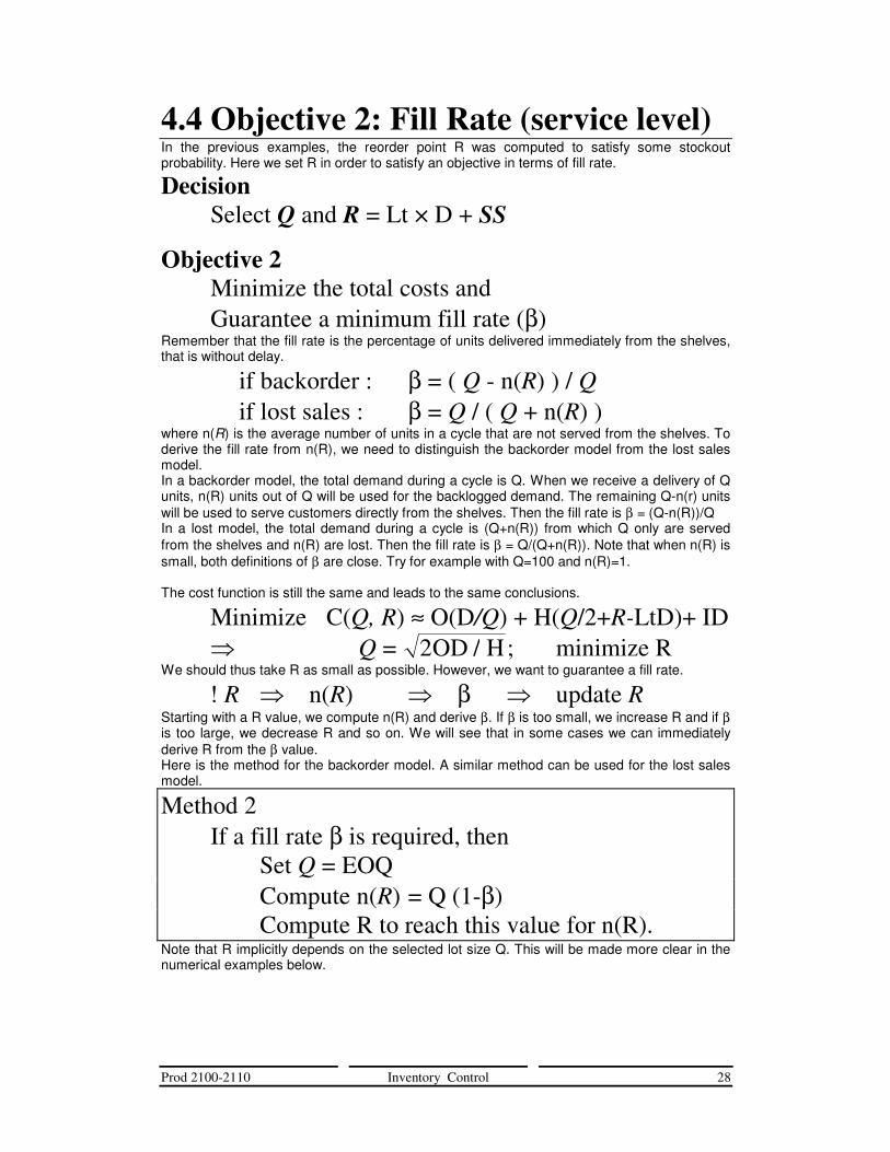
4.4 Objective 2: Fill Rate (service level) In the previous examples, the reorder point R was computed to satisfy some stockout probability. Here we set R in order to satisfy an objective in terms of fill rate.

Decision Select Q and R = Lt × D + SS

Objective 2 Minimize the total costs and Guarantee a minimum fill rate (β) Remember that the fill rate is the percentage of units delivered immediately from the shelves, that is without delay.

if backorder : β = ( Q - n(R) ) / Q if lost sales : β = Q / ( Q + n(R) )

where n(R) is the average number of units in a cycle that are not served from the shelves. To derive the fill rate from n(R), we need to distinguish the backorder model from the lost sales model. In a backorder model, the total demand during a cycle is Q. When we receive a delivery of Q units, n(R) units out of Q will be used for the backlogged demand. The remaining Q-n(r) units will be used to serve customers directly from the shelves. Then the fill rate is β = (Q-n(R))/Q In a lost model, the total demand during a cycle is (Q+n(R)) from which Q only are served from the shelves and n(R) are lost. Then the fill rate is β = Q/(Q+n(R)). Note that when n(R) is small, both definitions of β are close. Try for example with Q=100 and n(R)=1. The cost function is still the same and leads to the same conclusions.

Minimize C(Q, R) ≈ O(D/Q) + H(Q/2+R-LtD)+ ID � Q = 2OD / H; minimize R

We should thus take R as small as possible. However, we want to guarantee a fill rate.

! R � n(R) � β � update R Starting with a R value, we compute n(R) and derive β. If β is too small, we increase R and if β is too large, we decrease R and so on. We will see that in some cases we can immediately derive R from the β value. Here is the method for the backorder model. A similar method can be used for the lost sales model.

Method 2 If a fill rate β is required, then Set Q = EOQ Compute n(R) = Q (1-β) Compute R to reach this value for n(R). Note that R implicitly depends on the selected lot size Q. This will be made more clear in the numerical examples below.


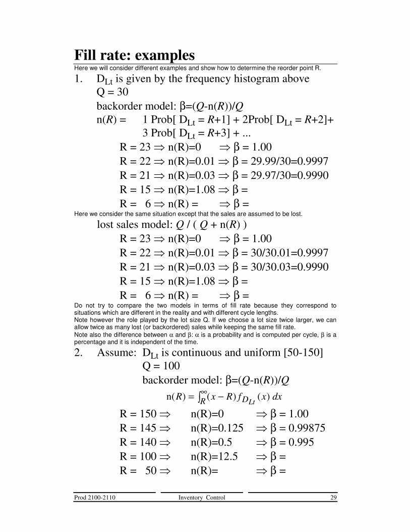
Fill rate: examples Here we will consider different examples and show how to determine the reorder point R.

1. DLt is given by the frequency histogram above Q = 30 backorder model: β=(Q-n(R))/Q

n(R) = 1 Prob[ DLt = R+1] + 2Prob[ DLt = R+2]+ 3 Prob[ DLt = R+3] + ...

R = 23 � n(R)=0 � β = 1.00 R = 22 � n(R)=0.01 � β = 29.99/30=0.9997 R = 21 � n(R)=0.03 � β = 29.97/30=0.9990 R = 15 � n(R)=1.08 � β = R = 6 � n(R) = � β =

Here we consider the same situation except that the sales are assumed to be lost.

lost sales model: Q / ( Q + n(R) ) R = 23 � n(R)=0 � β = 1.00 R = 22 � n(R)=0.01 � β = 30/30.01=0.9997 R = 21 � n(R)=0.03 � β = 30/30.03=0.9990 R = 15 � n(R)=1.08 � β = R = 6 � n(R) = � β =

Do not try to compare the two models in terms of fill rate because they correspond to situations which are different in the reality and with different cycle lengths. Note however the role played by the lot size Q. If we choose a lot size twice larger, we can allow twice as many lost (or backordered) sales while keeping the same fill rate. Note also the difference between α and β: α is a probability and is computed per cycle, β is a percentage and it is independent of the time.

2. Assume: DLt is continuous and uniform [50-150] Q = 100 backorder model: β=(Q-n(R))/Q

n( ) ( ) ( )R x R f x dxDR Lt= −∞

R = 150 � n(R)=0 � β = 1.00 R = 145 � n(R)=0.125 � β = 0.99875 R = 140 � n(R)=0.5 � β = 0.995 R = 100 � n(R)=12.5 � β = R = 50 � n(R)= � β =


Fill rate with the normal distribution Here we consider the normal distributions. Please refer, when needed, to the N(0,1) table given at the end of the section.

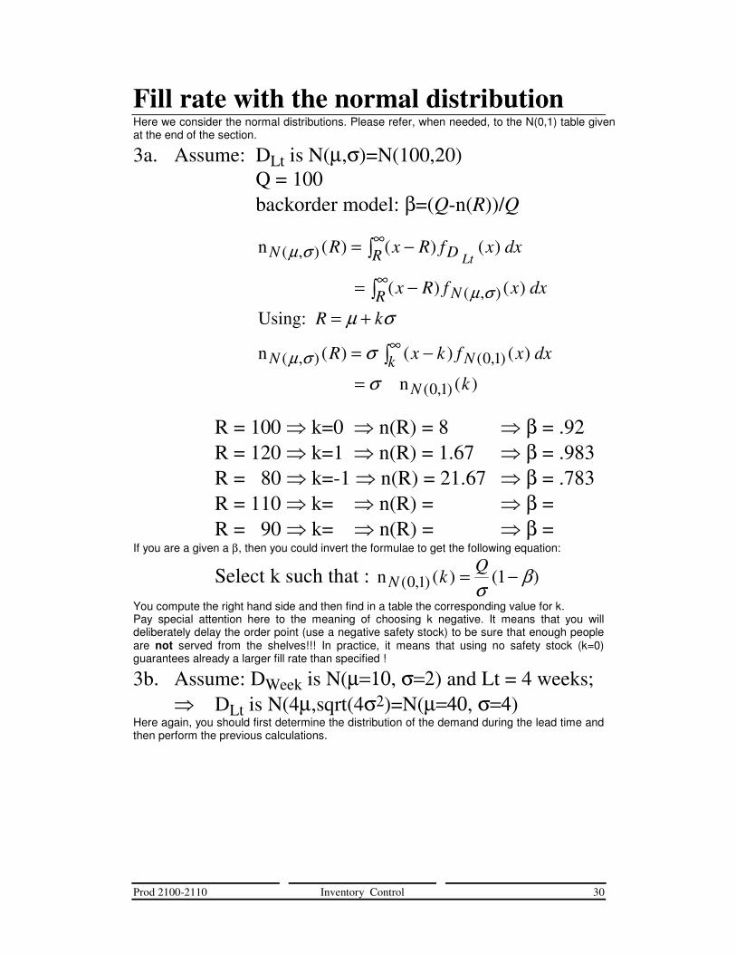
3a. Assume: DLt is N(µ,σ)=N(100,20) Q = 100 backorder model: β=(Q-n(R))/Q

n

Using:

n

n

N DR

NR

N Nk

N

R x R f x dx

x R f x dx

R k

R x k f x dx

k

Lt( , )

( , )

( , ) ( , )

( , )

( ) ( ) ( )

( ) ( )

( ) ( ) ( )

( )

µ σ

µ σ

µ σ

µ σ

σσ

= −

= −

= +

= −

=

∞

∞

∞

0 1

0 1

R = 100 � k=0 � n(R) = 8 � β = .92 R = 120 � k=1 � n(R) = 1.67 � β = .983 R = 80 � k=-1 � n(R) = 21.67 � β = .783 R = 110 � k= � n(R) = � β = R = 90 � k= � n(R) = � β =

If you are a given a β, then you could invert the formulae to get the following equation:

Select k such that : nN kQ

( , ) ( ) ( )0 1 1= −σ

β You compute the right hand side and then find in a table the corresponding value for k. Pay special attention here to the meaning of choosing k negative. It means that you will deliberately delay the order point (use a negative safety stock) to be sure that enough people are not served from the shelves!!! In practice, it means that using no safety stock (k=0) guarantees already a larger fill rate than specified !

3b. Assume: DWeek is N(µ=10, σ=2) and Lt = 4 weeks; � DLt is N(4µ,sqrt(4σ2)=N(µ=40, σ=4) Here again, you should first determine the distribution of the demand during the lead time and then perform the previous calculations.


4.5 Objective 3: Minimize the total costs In the previous examples, R was computed to fulfill some service performance.

Decision: Select Q and R = Lt × D + SS

Here a pure economical analysis is carried on.

Objective 3 Minimize the total costs assuming penalty costs for the demand which cannot be served from stock.

Here we assume that each unit which is demanded and which cannot be immediately served generates a cost P.

Penalty Costs: P (money/unit) �� lost profit / contractual penalty / loss of goodwill

The determination of the penalty cost is difficult in practice. Here are some examples. If you sell newspapers on the street, and if you run out of stock, for each unit you do not sell, you loose the corresponding profit. If you are a baker and you run out of breads. Not only you loose the profit associated with each bread, but you could also loose a customer.

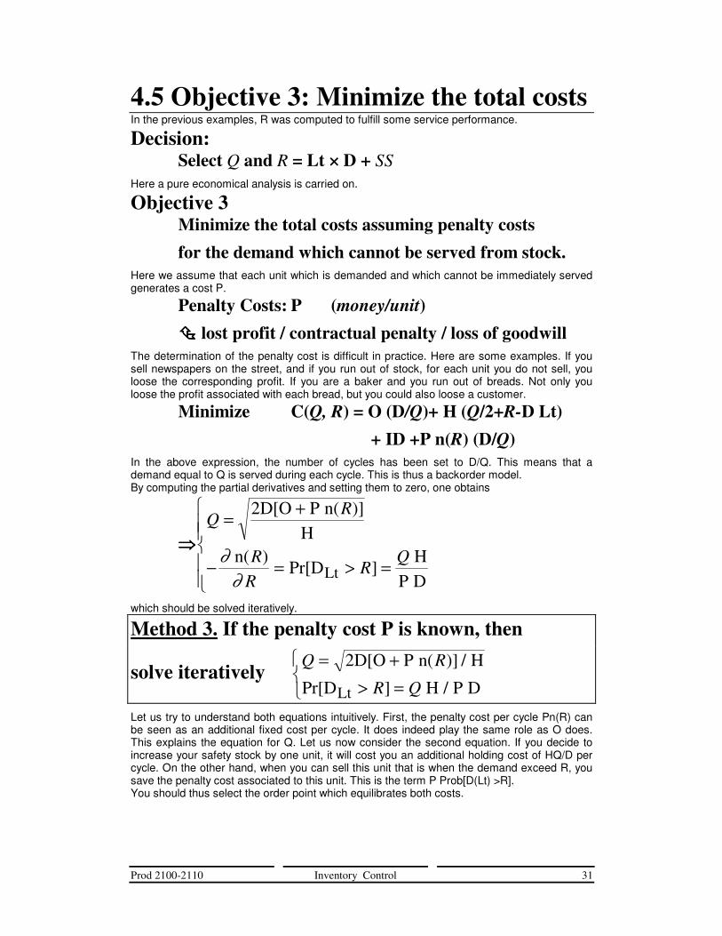
Minimize C(Q, R) = O (D/Q)+ H (Q/2+R-D Lt) + ID +P n(R) (D/Q)

In the above expression, the number of cycles has been set to D/Q. This means that a demand equal to Q is served during each cycle. This is thus a backorder model. By computing the partial derivatives and setting them to zero, one obtains

��

QR

RR

RQ

= +

− = > =

��

��

2D[O P n( )]H

n( )Pr[D ]

HP DLt

∂∂

which should be solved iteratively.

Method 3. If the penalty cost P is known, then

solve iteratively Q R

R Q

= +> =

�

2D[O P n( )] / H

Pr[D ] H / P D Lt

Let us try to understand both equations intuitively. First, the penalty cost per cycle Pn(R) can be seen as an additional fixed cost per cycle. It does indeed play the same role as O does. This explains the equation for Q. Let us now consider the second equation. If you decide to increase your safety stock by one unit, it will cost you an additional holding cost of HQ/D per cycle. On the other hand, when you can sell this unit that is when the demand exceed R, you save the penalty cost associated to this unit. This is the term P Prob[D(Lt) >R]. You should thus select the order point which equilibrates both costs.


Penalty Costs: examples Here we will consider different examples and show how to determine the reorder point R.

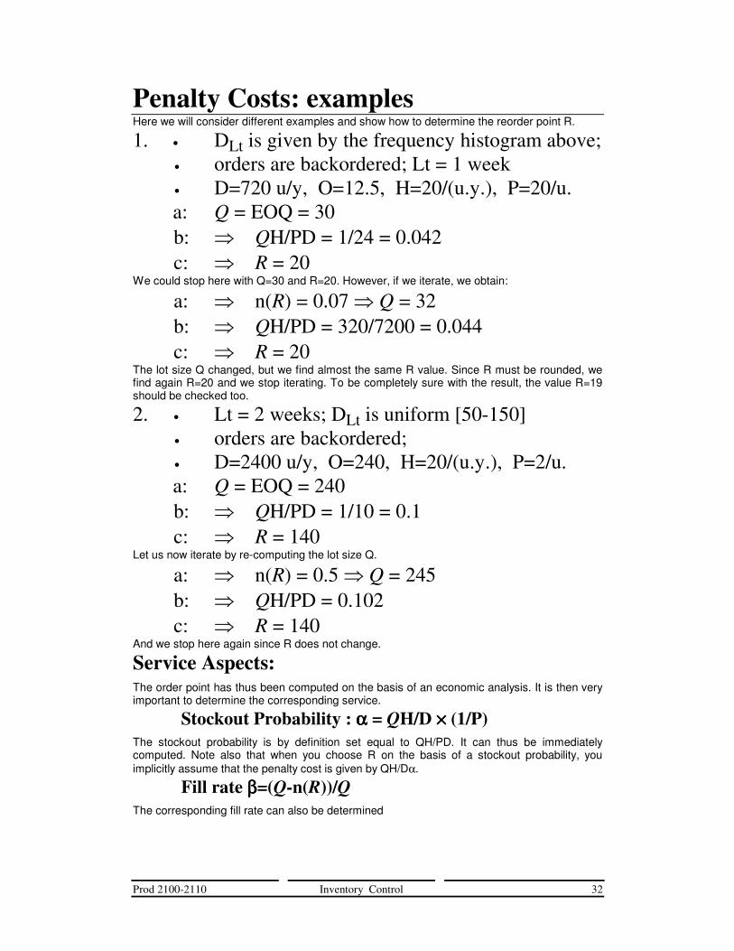
1. • DLt is given by the frequency histogram above; • orders are backordered; Lt = 1 week • D=720 u/y, O=12.5, H=20/(u.y.), P=20/u. a: Q = EOQ = 30 b: � QH/PD = 1/24 = 0.042 c: � R = 20

We could stop here with Q=30 and R=20. However, if we iterate, we obtain:

a: � n(R) = 0.07 � Q = 32 b: � QH/PD = 320/7200 = 0.044 c: � R = 20

The lot size Q changed, but we find almost the same R value. Since R must be rounded, we find again R=20 and we stop iterating. To be completely sure with the result, the value R=19 should be checked too.

2. • Lt = 2 weeks; DLt is uniform [50-150] • orders are backordered; • D=2400 u/y, O=240, H=20/(u.y.), P=2/u. a: Q = EOQ = 240 b: � QH/PD = 1/10 = 0.1 c: � R = 140

Let us now iterate by re-computing the lot size Q.

a: � n(R) = 0.5 � Q = 245 b: � QH/PD = 0.102 c: � R = 140

And we stop here again since R does not change.

Service Aspects: The order point has thus been computed on the basis of an economic analysis. It is then very important to determine the corresponding service.

Stockout Probability : αααα = QH/D ×××× (1/P) The stockout probability is by definition set equal to QH/PD. It can thus be immediately computed. Note also that when you choose R on the basis of a stockout probability, you implicitly assume that the penalty cost is given by QH/Dα.

Fill rate ββββ=(Q-n(R))/Q The corresponding fill rate can also be determined


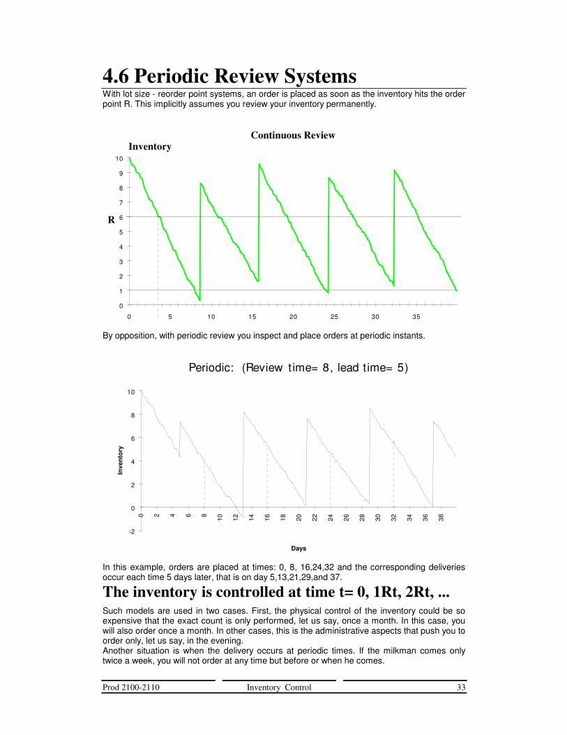
4.6 Periodic Review Systems With lot size - reorder point systems, an order is placed as soon as the inventory hits the order point R. This implicitly assumes you review your inventory permanently.

Continuous Review

0

1

2

3

4

5

6

7

8

9

10

0 5 10 15 20 25 30 35

Inventory

R

By opposition, with periodic review you inspect and place orders at periodic instants.

Periodic: (Review t ime= 8, lead time= 5)

Days

Inve

ntor

y

-2

0

2

4

6

8

10

0 2 4 6 8

10 12 14 16 18 20 22 24 26 28 30 32 34 36 38

In this example, orders are placed at times: 0, 8, 16,24,32 and the corresponding deliveries occur each time 5 days later, that is on day 5,13,21,29,and 37.

The inventory is controlled at time t= 0, 1Rt, 2Rt, ... Such models are used in two cases. First, the physical control of the inventory could be so expensive that the exact count is only performed, let us say, once a month. In this case, you will also order once a month. In other cases, this is the administrative aspects that push you to order only, let us say, in the evening. Another situation is when the delivery occurs at periodic times. If the milkman comes only twice a week, you will not order at any time but before or when he comes.


Periodic Review Let us try to summarize the ins and outs of the problem.

Assumptions 1. Constant random demand: D 2. Lead time (Lt > 0) 3. Review time (Rt > 0)

Costs holding costs: H money / (item . time) order costs: O (money) penalty costs: P (money / item)

Service Stockout frequency f or Fill rate ββββ

We are given either some penalty cost to minimize or a service level or fill rate to reach.

Decision Select Qi

Most often the lot size is not kept constant and you are allowed to order a quantity which depends on the current state of your inventory. However, there are cases where the order lot size is fixed. This happens typically when the review period is short (one day, for example).

Objective Minimize the total costs or Guarantee a service

Since we have only one variable, we cannot aim at different objectives at the same time. Let us consider briefly two cases.


1. Cost Minimization For facility reasons, we can address the following questions sequentially:

When to order: at every Rt or less often ? This question can be easily solved by compromising the holding costs and the order costs. A reasonable goal consists in ordering at the frequency close to that of the EOQ model. Given now the ordering frequency, we can proceed.

How much to order ? The answer is: enough to cover the average demand till the next delivery plus some safety stock. The “time till the next delivery” must be clearly identified.

1. Vulnerability Period = Review time + Lead time Let us consider the example of previous page again. At time 0, we observe some inventory, let us say 10 and we decide to order some quantity, let us say 3. After we have placed this order, we cannot interfere with our inventory before time 13! Indeed, the earliest time we can order again is time 8 and we will be delivered 5 days (the lead time) later. In another words, when we place our order for 3 units, then we cannot modify the evolution of the inventory up to time 13. This is the “vulnerability period” in this case. Let us consider the items which will be used to cover the demand during this vulnerability period. We observed an inventory of 10 units and we ordered 3 units. Altogether, these 13 units will be used to cover the demand during these 13 days.

2. Demand (Vulnerability Period) = DVp 3. Safety stock

Once the demand over the vulnerability period is known, we can chose a safety stock. For example, in the previous example, the demand over 13 days has a mean of 13 with some variation. In the simulation, no safety stock was used. The calculation of a safety stock which aims at meeting some service performance is described next. However, a pure cost minimization objective can be pursued if the penalty cost associated with a stockout can be estimated.


2. Maximum Stockout frequency Let us for example try to select a policy which guarantees a maximum stockout frequency. On the chart, at time 0 we have an inventory, let us say Io units, and we ordered some quantity, let us say Qo. All these (Io + Qo ) units will be used to serve the demand up to time (13 = Vp). The probability of stocking out is thus the probability that the demand during this time exceeds these (Io + Qo ) units. The reasoning can be repeated at time 8. We thus have

Stockout Probability = Prob[ DVp > Ii + Qi ]

where DVp is the demand during Vp Ii is the inventory at observation i Qi is the quantity ordered at i

We should thus define the quantity I(i)+Q(i) that will be used to serve the demand during the vulnerability period. Let us firs assume that this demand is normally distributed.

Assume DVp is N(µµµµVp,σσσσVp) In this case we can choose to cover the average demand and take some standard deviations of this demand as safety stock.

Choose: Qi = µµµµVp + k σσσσVp - Ii = Qmax - Ii With, for example k =1, we have a 16 percent probability of stocking out in each cycle. If we order every 8 days, the average stockout frequency over a year is 0.16 * 365/8 = 7.2 stockouts per year. Please, pay attention to the difference between the vulnerability period and the time between two “risky” periods, that is the time between two orders. With a fill rate objective, a similar procedure can be followed.


4.7 Lead Time Variability Up to now we always assumed that the demand during the lead time was known or that it could be determined from the knowledge of the lead time itself and of the distribution of the demand during a known period. Here we consider the case where the lead time itself is also variable.

Lead Time parameters �� lead time Lt is a random variable with:

mean: E[Lt] variance: VAR[Lt]

In the previous pages, we assumed the lead time to be deterministic, that is with variance 0. Now we assume it has some positive variance.

Demand Parameters �� demand during t days is a random variable with: mean: t E[Dday] variance: t Var[Dday]

This means the demand over t days is the sum of t daily demands. It has an average equal to t times the average daily demand and a variance equal to t times the variance of the daily demand.

� Demand during lead time is a random variable with: mean: µ µ µ µ = E[Lt] E[Dday] variance: σσσσ2=E[Lt]Var[Dday] + E2[Dday]Var[Lt]

Verification: if VAR[Lt] = 0, then σ2= E[Lt] Var[Dday] (a sum of E[Lt] identical random variables) This case is as before. The lead time is constant and the demand during the lead time is the sum of daily demands over "lead time" days. The variance of a sum equals the sum of variances.

if VAR[Dday] = 0, then σ2 =E2[Dday] VAR[Lt] the random variable "demand during lead time" = = random variable "lead time length" ×λ This case is new. The daily demand is fixed. The lead time is variable. The distribution of the demand during the lead time is equal to the distribution of the lead time after an appropriate scaling. The days are replaced by demand units. You use here the rule : var(k times a random variable X) = k*k var(X).


5. Multiproduct Systems: ABC Analysis Here we consider the classical case of a company with many different products and components to manage. Before trying to define any inventory control policy, the first step is to conduct an ABC analysis (also called Pareto analysis) which aims at determining where the money is spent. Such an analysis is required to determine on which product you will spend your effort improving the inventory control.

1. Select a discriminating characteristics ex.: demand volume / sales volume / profit volume

When dealing with inventories, the sales volume is a good criterion.

2. Rank the products according to this characteristic ex.: product 1 has the highest sales volume; product 2 has the second highest sales volume; ...

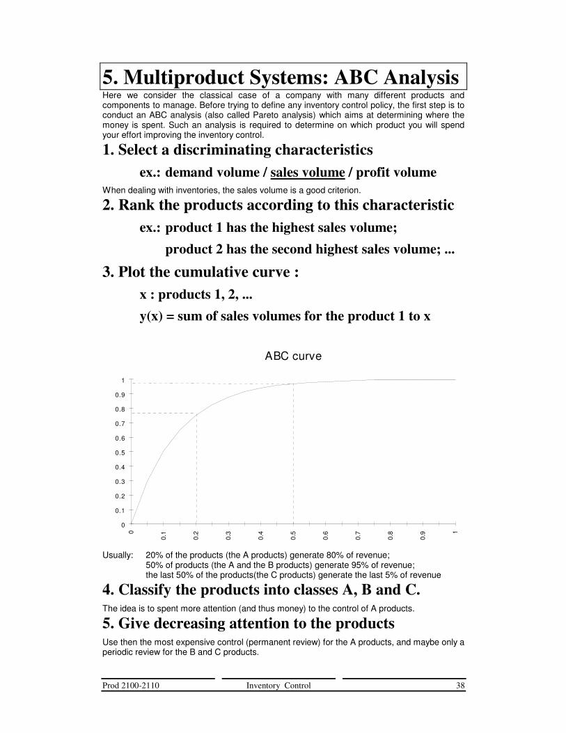
3. Plot the cumulative curve : x : products 1, 2, ... y(x) = sum of sales volumes for the product 1 to x

ABC curve

0

0.1

0.2

0.3

0.4

0.5

0.6

0.7

0.8

0.9

1

0

0.1

0.2

0.3

0.4

0.5

0.6

0.7

0.8

0.9 1

Usually: 20% of the products (the A products) generate 80% of revenue; 50% of products (the A and the B products) generate 95% of revenue; the last 50% of the products(the C products) generate the last 5% of revenue

4. Classify the products into classes A, B and C. The idea is to spent more attention (and thus money) to the control of A products.

5. Give decreasing attention to the products Use then the most expensive control (permanent review) for the A products, and maybe only a periodic review for the B and C products.


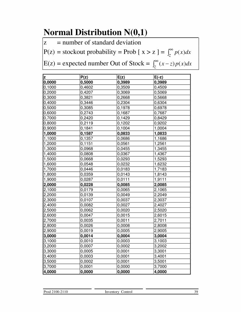
Normal Distribution N(0,1) z = number of standard deviation P(z) = stockout probability = Prob [ x > z ] = p x dxz

∞ ( )

E(z) = expected number Out of Stock = ( ) ( )x z p x dxz −∞

z P(z) E(z) E(-z) 0,0000 0,5000 0,3989 0,3989 0,1000 0,4602 0,3509 0,4509 0,2000 0,4207 0,3069 0,5069 0,3000 0,3821 0,2668 0,5668 0,4000 0,3446 0,2304 0,6304 0,5000 0,3085 0,1978 0,6978 0,6000 0,2743 0,1687 0,7687 0,7000 0,2420 0,1429 0,8429 0,8000 0,2119 0,1202 0,9202 0,9000 0,1841 0,1004 1,0004 1,0000 0,1587 0,0833 1,0833 1,1000 0,1357 0,0686 1,1686 1,2000 0,1151 0,0561 1,2561 1,3000 0,0968 0,0455 1,3455 1,4000 0,0808 0,0367 1,4367 1,5000 0,0668 0,0293 1,5293 1,6000 0,0548 0,0232 1,6232 1,7000 0,0446 0,0183 1,7183 1,8000 0,0359 0,0143 1,8143 1,9000 0,0287 0,0111 1,9111 2,0000 0,0228 0,0085 2,0085 2,1000 0,0179 0,0065 2,1065 2,2000 0,0139 0,0049 2,2049 2,3000 0,0107 0,0037 2,3037 2,4000 0,0082 0,0027 2,4027 2,5000 0,0062 0,0020 2,5020 2,6000 0,0047 0,0015 2,6015 2,7000 0,0035 0,0011 2,7011 2,8000 0,0026 0,0008 2,8008 2,9000 0,0019 0,0005 2,9005 3,0000 0,0014 0,0004 3,0004 3,1000 0,0010 0,0003 3,1003 3,2000 0,0007 0,0002 3,2002 3,3000 0,0005 0,0001 3,3001 3,4000 0,0003 0,0001 3,4001 3,5000 0,0002 0,0001 3,5001 3,7000 0,0001 0,0000 3,7000 4,0000 0,0000 0,0000 4,0000

Documents

Inventory Control - POMS