S-1

SUPPLEMENTAL INFORMATION FOR THE MANUSCRIPT

The ATAD2 bromodomain binds different acetylation marks on the histone H4 in similar fuzzy complexes

Cassiano Langini, Amedeo Caflisch, Andreas Vitalis

INVENTORY OF SUPPLEMENTAL INFORMATION

SUPPLEMENTAL METHODS

Additional simulation details

Details of Monte Carlo procedure for preparation of holo starting structures

Additional analysis details

SUPPLEMENTAL TABLES

Table S1

SUPPLEMENTAL FIGURES

Figures S1-S12

SUPPLEMENTAL MOVIE CAPTIONS

Movie S1

SUPPLEMENTAL REFERENCES

SUPPLEMENTAL METHODS Additional simulation details We used a standard molecular dynamics methodology as follows. To reproduce neutral pH conditions, side chains of D/E were negatively charged, those of K/R were positively charged, and H was kept neutral (with the hydrogen always on Nε). We introduced both N- and C-terminal caps for ATAD2A and only a C-terminal cap for the histone H4-derived peptide. The peptide-bound structures were solvated in rectangular, periodic boxes of sizes 110x70x70Å3. To prevent image interactions of the peptide with more than one protein, the protein’s long dimension was kept aligned with that of the box by harmonic restraints on the Cα atoms of residues L1050 and R1075, which practically eliminate tumbling (k = 1000kJmol-1nm-2). For simulations of the free domain, the two position restraints were retained but a smaller cubic box of 85Å side length was used. The simulation system contained K+ and CL- ions to approximate an ionic strength of 150mM and compensate for the total charge of the solutes. The simulations were performed with GROMACS 5.0 (1) using the CHARMM36 force field (2) and modified TIP3P water model (3). Electrostatic interactions were evaluated using the generalized reaction-field method (4), and truncation of all nonbonded interactions occurred at 12Å. Simulations were performed in the NVT ensemble with the temperature of 310K kept constant by an external bath with velocity rescaling (5) and a coupling time of 2ps. The LINCS

S-2

algorithm was used to constrain all covalent bonds (6). The integration time step was 2fs, and snapshots were saved every 20ps. The simulations of the free peptide differed in that they used a smaller cubic box of ca. 60Å side length at 1atm pressure in the NPT ensemble. Pressure was maintained by the Berendsen manostat (7) with a coupling time of 2ps. The lengths and starting conditions for all simulations are summarized in Fig. 1c in the main text. The set of starting conformations for the peptide-only simulations were extracted from a clustering of the data underlying Fig. 2a-b in the main text. This procedure ensured that a wide range of initial shapes and sizes was present initially. Snapshots were saved every 10ps for the free peptide simulations. Details of Monte Carlo procedure for preparation of holo starting structures In order to generate starting conformations with the peptide bound, we needed to reconstruct and relax peptide conformations for which we employed a Metropolis Monte Carlo sampler in torsional space as implemented in CAMPARIv2 (http://campari.sourceforge.net). A key-file replicating the exact move set we used is available from the authors on request. Move set details are omitted here because they are inconsequential. The MC relaxation runs were made to preserve the orientation of the crystallographic pose inasmuch as it was resolved. To achieve this, we utilized the distance restraints summarized in Table S1. The MC simulation was run for 106 elementary steps for either Kac5 or Kac12 being inserted. In each case, structures were extracted every 105 steps. Relaxation of the peptide occurred in the absence of solvent and using only Lennard-Jones interactions with ABSINTH parameters (8), which are suitable for the dihedral angle-based sampling we employed. This procedure generated 10 clash-free structures for either holo case, which were ready to be solvated by, in this order, compatible crystal waters (i.e., crystal waters not closer than 3Å to the newly built residues of the peptide) and then by the GROMACS utility gmx solvate. A thin solvation layer (water molecules with oxygen closer than 2Å to either protein, ligand or crystal water atoms) was removed to avoid steric clashes and wrong positioning of water molecules inside the bulk of the bromodomain. This procedure required the subsequent equilibration in the NPT ensemble to recover the correct volume and density of the system. Additional analysis details To produce the SAPPHIRE plots, we needed to calculate the underlying sequence of snapshots, i.e., the progress index. This requires fundamentally only the specification of a metric to calculate snapshot-to-snapshot distances. The root mean square deviation (RMSD) metric (Fig. 6) was defined as the Euclidean distance between the absolute coordinates of the N, O, and Cβ atoms of the non-proline residues from D1003–D1030 (ZA loop) and Y1063–D1068 (BC loop) and the O and Cβ atoms of residues P1012, P1015, P1019, P1028, P1065, and P1069 (99 atoms in total). The distance was calculated after alignment on the Cα atoms of the residues comprising helices αZ, αA, αB, and αC, which excludes the short, unlabeled C-terminal helix in Fig. 1a. The dihedral angle-based metric (Fig. S12 and Fig. 8d in the main text) was composed of the 108 sine and cosine values of the φ- and ψ-angles of residues K1004 to D1030. There are no BC loop residues in this set because of the observed lack of backbone heterogeneity in Fig. 4. Because of the data set size we resorted to the approximate method as published (9). In this, the data are preorganized by a tree-based clustering (10) to simplify the search for the next candidates. The settings for this tree-based clustering were as follows. For the coordinate

S-3

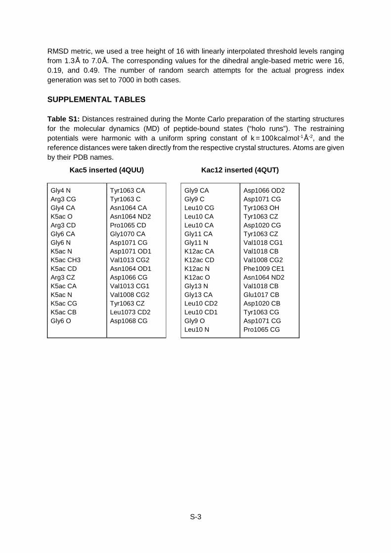
RMSD metric, we used a tree height of 16 with linearly interpolated threshold levels ranging from 1.3Å to 7.0Å. The corresponding values for the dihedral angle-based metric were 16, 0.19, and 0.49. The number of random search attempts for the actual progress index generation was set to 7000 in both cases. SUPPLEMENTAL TABLES Table S1: Distances restrained during the Monte Carlo preparation of the starting structures for the molecular dynamics (MD) of peptide-bound states (“holo runs”). The restraining potentials were harmonic with a uniform spring constant of k = 100kcalmol-1Å-2, and the reference distances were taken directly from the respective crystal structures. Atoms are given by their PDB names.

Kac5 inserted (4QUU) Kac12 inserted (4QUT)

Gly4 N Arg3 CG Gly4 CA K5ac O Arg3 CD Gly6 CA Gly6 N K5ac N K5ac CH3 K5ac CD Arg3 CZ K5ac CA K5ac N K5ac CG K5ac CB Gly6 O

Tyr1063 CA Tyr1063 C Asn1064 CA Asn1064 ND2 Pro1065 CD Gly1070 CA Asp1071 CG Asp1071 OD1 Val1013 CG2 Asn1064 OD1 Asp1066 CG Val1013 CG1 Val1008 CG2 Tyr1063 CZ Leu1073 CD2 Asp1068 CG

Gly9 CA Gly9 C Leu10 CG Leu10 CA Leu10 CA Gly11 CA Gly11 N K12ac CA K12ac CD K12ac N K12ac O Gly13 N Gly13 CA Leu10 CD2 Leu10 CD1 Gly9 O Leu10 N

Asp1066 OD2 Asp1071 CG Tyr1063 OH Tyr1063 CZ Asp1020 CG Tyr1063 CZ Val1018 CG1 Val1018 CB Val1008 CG2 Phe1009 CE1 Asn1064 ND2 Val1018 CB Glu1017 CB Asp1020 CB Tyr1063 CG Asp1071 CG Pro1065 CG

S-4

SUPPLEMENTAL FIGURES

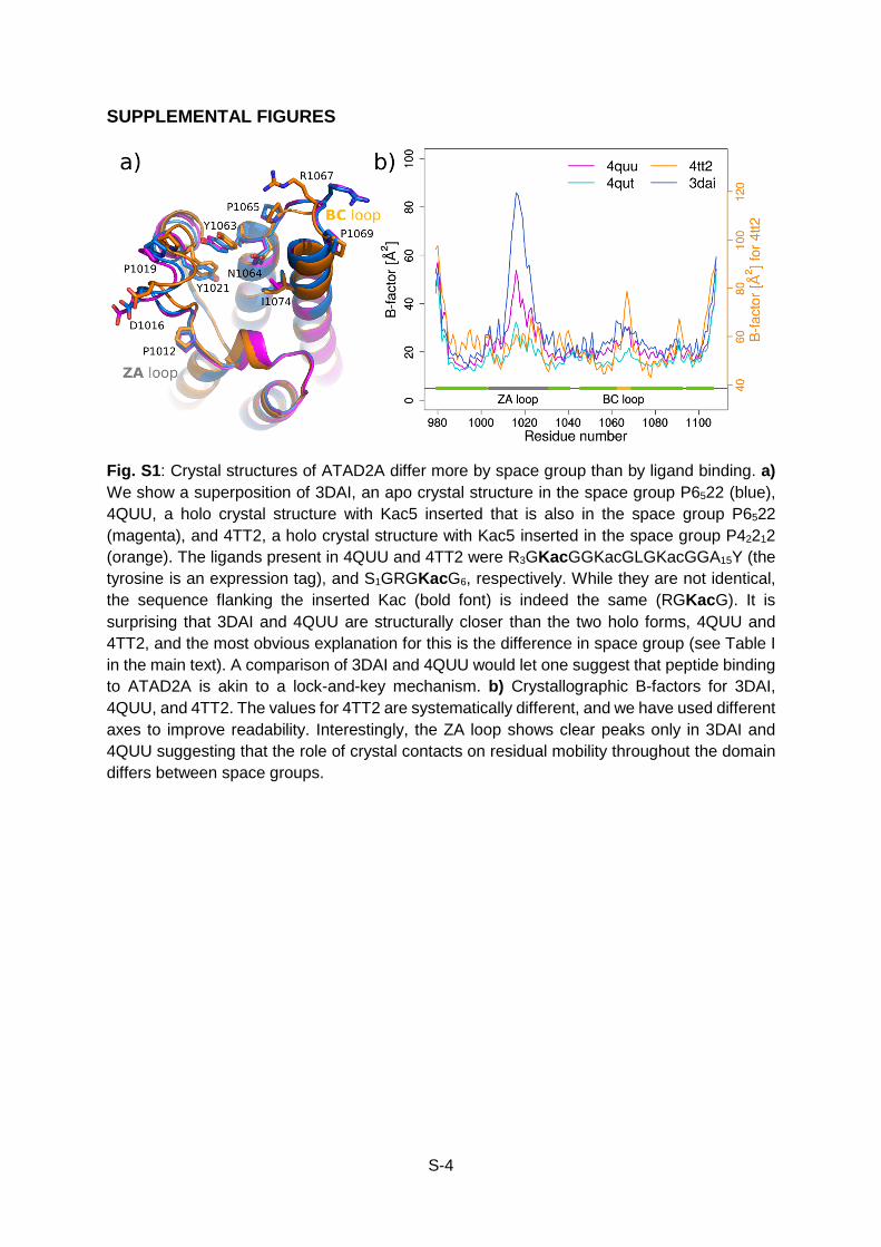
Fig. S1: Crystal structures of ATAD2A differ more by space group than by ligand binding. a) We show a superposition of 3DAI, an apo crystal structure in the space group P6522 (blue), 4QUU, a holo crystal structure with Kac5 inserted that is also in the space group P6522 (magenta), and 4TT2, a holo crystal structure with Kac5 inserted in the space group P42212 (orange). The ligands present in 4QUU and 4TT2 were R3GKacGGKacGLGKacGGA15Y (the tyrosine is an expression tag), and S1GRGKacG6, respectively. While they are not identical, the sequence flanking the inserted Kac (bold font) is indeed the same (RGKacG). It is surprising that 3DAI and 4QUU are structurally closer than the two holo forms, 4QUU and 4TT2, and the most obvious explanation for this is the difference in space group (see Table I in the main text). A comparison of 3DAI and 4QUU would let one suggest that peptide binding to ATAD2A is akin to a lock-and-key mechanism. b) Crystallographic B-factors for 3DAI, 4QUU, and 4TT2. The values for 4TT2 are systematically different, and we have used different axes to improve readability. Interestingly, the ZA loop shows clear peaks only in 3DAI and 4QUU suggesting that the role of crystal contacts on residual mobility throughout the domain differs between space groups.

S-5

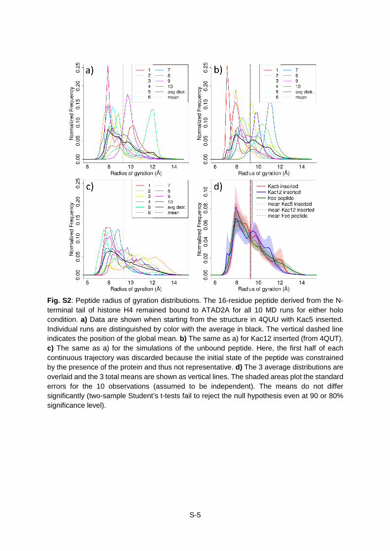
Fig. S2: Peptide radius of gyration distributions. The 16-residue peptide derived from the N-terminal tail of histone H4 remained bound to ATAD2A for all 10 MD runs for either holo condition. a) Data are shown when starting from the structure in 4QUU with Kac5 inserted. Individual runs are distinguished by color with the average in black. The vertical dashed line indicates the position of the global mean. b) The same as a) for Kac12 inserted (from 4QUT). c) The same as a) for the simulations of the unbound peptide. Here, the first half of each continuous trajectory was discarded because the initial state of the peptide was constrained by the presence of the protein and thus not representative. d) The 3 average distributions are overlaid and the 3 total means are shown as vertical lines. The shaded areas plot the standard errors for the 10 observations (assumed to be independent). The means do not differ significantly (two-sample Student’s t-tests fail to reject the null hypothesis even at 90 or 80% significance level).

S-6

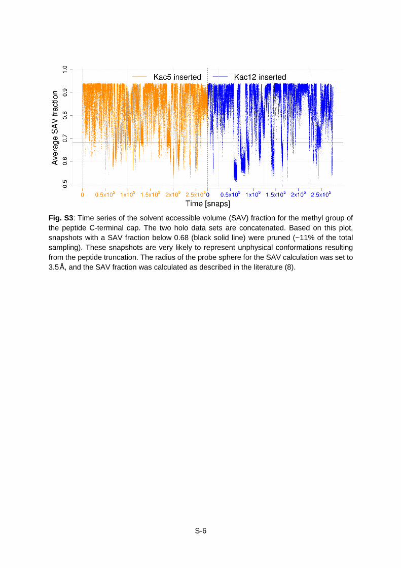
Fig. S3: Time series of the solvent accessible volume (SAV) fraction for the methyl group of the peptide C-terminal cap. The two holo data sets are concatenated. Based on this plot, snapshots with a SAV fraction below 0.68 (black solid line) were pruned (~11% of the total sampling). These snapshots are very likely to represent unphysical conformations resulting from the peptide truncation. The radius of the probe sphere for the SAV calculation was set to 3.5Å, and the SAV fraction was calculated as described in the literature (8).

S-7

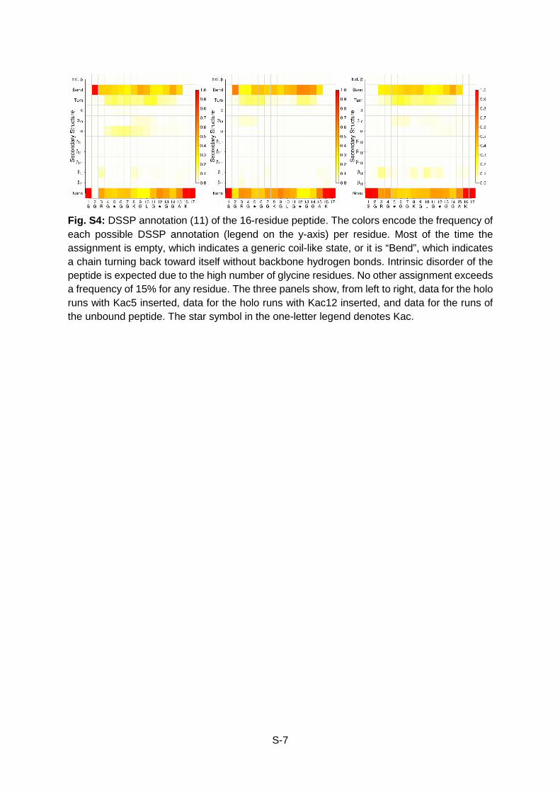
Fig. S4: DSSP annotation (11) of the 16-residue peptide. The colors encode the frequency of each possible DSSP annotation (legend on the y-axis) per residue. Most of the time the assignment is empty, which indicates a generic coil-like state, or it is “Bend”, which indicates a chain turning back toward itself without backbone hydrogen bonds. Intrinsic disorder of the peptide is expected due to the high number of glycine residues. No other assignment exceeds a frequency of 15% for any residue. The three panels show, from left to right, data for the holo runs with Kac5 inserted, data for the holo runs with Kac12 inserted, and data for the runs of the unbound peptide. The star symbol in the one-letter legend denotes Kac.

S-8

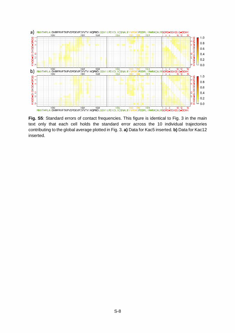
Fig. S5: Standard errors of contact frequencies. This figure is identical to Fig. 3 in the main text only that each cell holds the standard error across the 10 individual trajectories contributing to the global average plotted in Fig. 3. a) Data for Kac5 inserted. b) Data for Kac12 inserted.

S-9

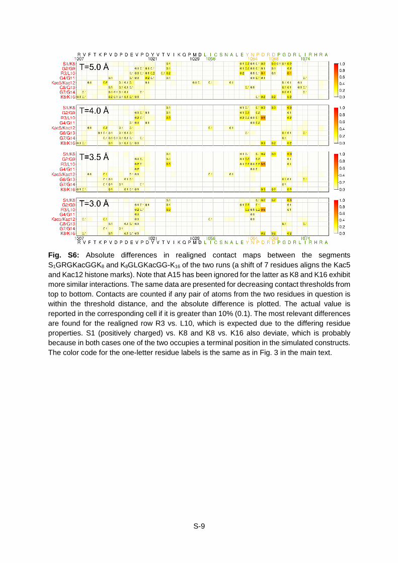
Fig. S6: Absolute differences in realigned contact maps between the segments S1GRGKacGGK8 and K8GLGKacGG-K16 of the two runs (a shift of 7 residues aligns the Kac5 and Kac12 histone marks). Note that A15 has been ignored for the latter as K8 and K16 exhibit more similar interactions. The same data are presented for decreasing contact thresholds from top to bottom. Contacts are counted if any pair of atoms from the two residues in question is within the threshold distance, and the absolute difference is plotted. The actual value is reported in the corresponding cell if it is greater than 10% (0.1). The most relevant differences are found for the realigned row R3 vs. L10, which is expected due to the differing residue properties. S1 (positively charged) vs. K8 and K8 vs. K16 also deviate, which is probably because in both cases one of the two occupies a terminal position in the simulated constructs. The color code for the one-letter residue labels is the same as in Fig. 3 in the main text.

S-10

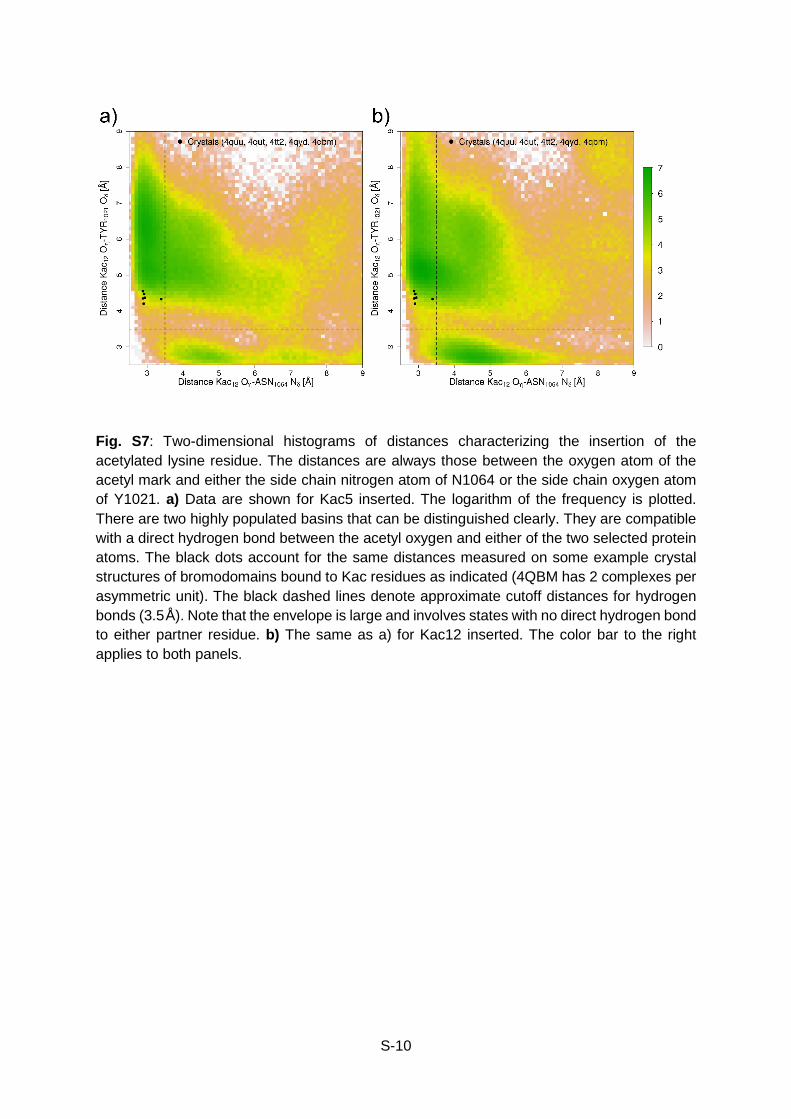
Fig. S7: Two-dimensional histograms of distances characterizing the insertion of the acetylated lysine residue. The distances are always those between the oxygen atom of the acetyl mark and either the side chain nitrogen atom of N1064 or the side chain oxygen atom of Y1021. a) Data are shown for Kac5 inserted. The logarithm of the frequency is plotted. There are two highly populated basins that can be distinguished clearly. They are compatible with a direct hydrogen bond between the acetyl oxygen and either of the two selected protein atoms. The black dots account for the same distances measured on some example crystal structures of bromodomains bound to Kac residues as indicated (4QBM has 2 complexes per asymmetric unit). The black dashed lines denote approximate cutoff distances for hydrogen bonds (3.5Å). Note that the envelope is large and involves states with no direct hydrogen bond to either partner residue. b) The same as a) for Kac12 inserted. The color bar to the right applies to both panels.

S-11

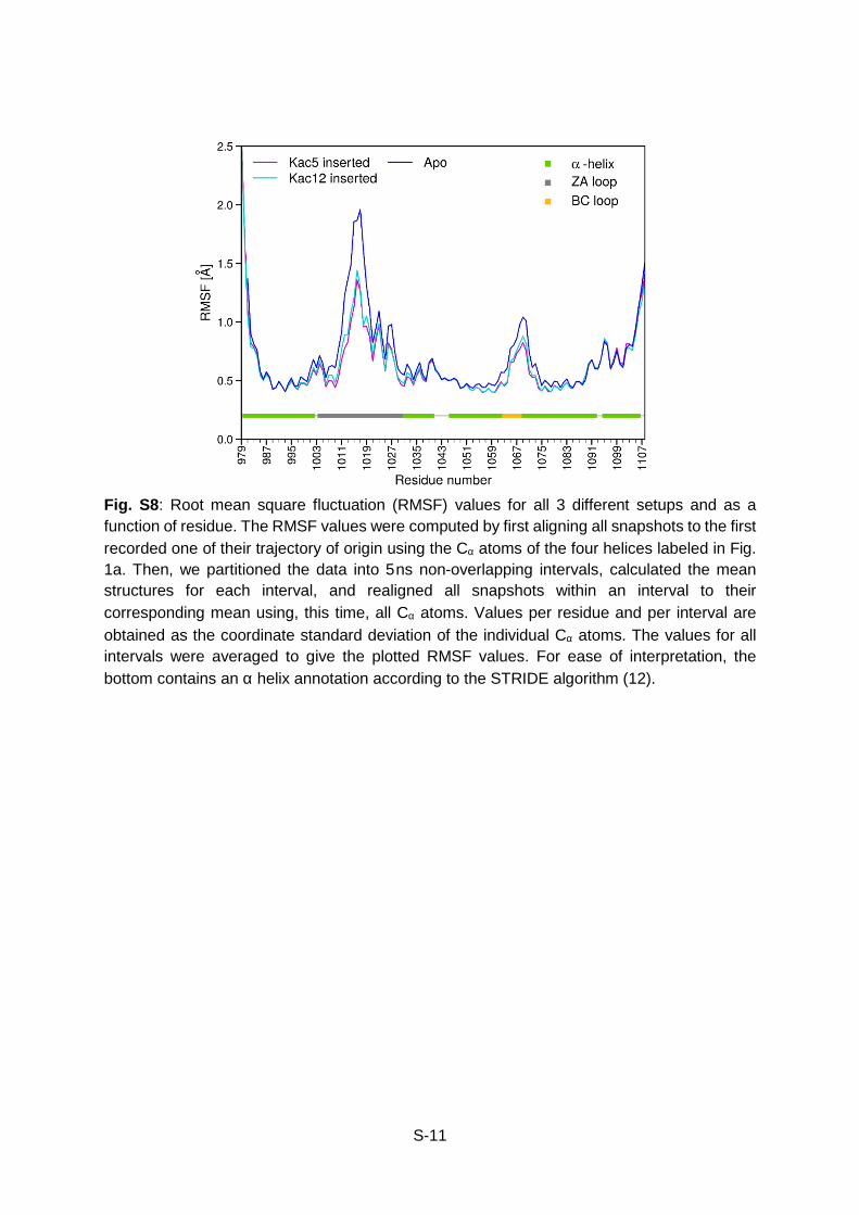
Fig. S8: Root mean square fluctuation (RMSF) values for all 3 different setups and as a function of residue. The RMSF values were computed by first aligning all snapshots to the first recorded one of their trajectory of origin using the Cα atoms of the four helices labeled in Fig. 1a. Then, we partitioned the data into 5ns non-overlapping intervals, calculated the mean structures for each interval, and realigned all snapshots within an interval to their corresponding mean using, this time, all Cα atoms. Values per residue and per interval are obtained as the coordinate standard deviation of the individual Cα atoms. The values for all intervals were averaged to give the plotted RMSF values. For ease of interpretation, the bottom contains an α helix annotation according to the STRIDE algorithm (12).

S-12

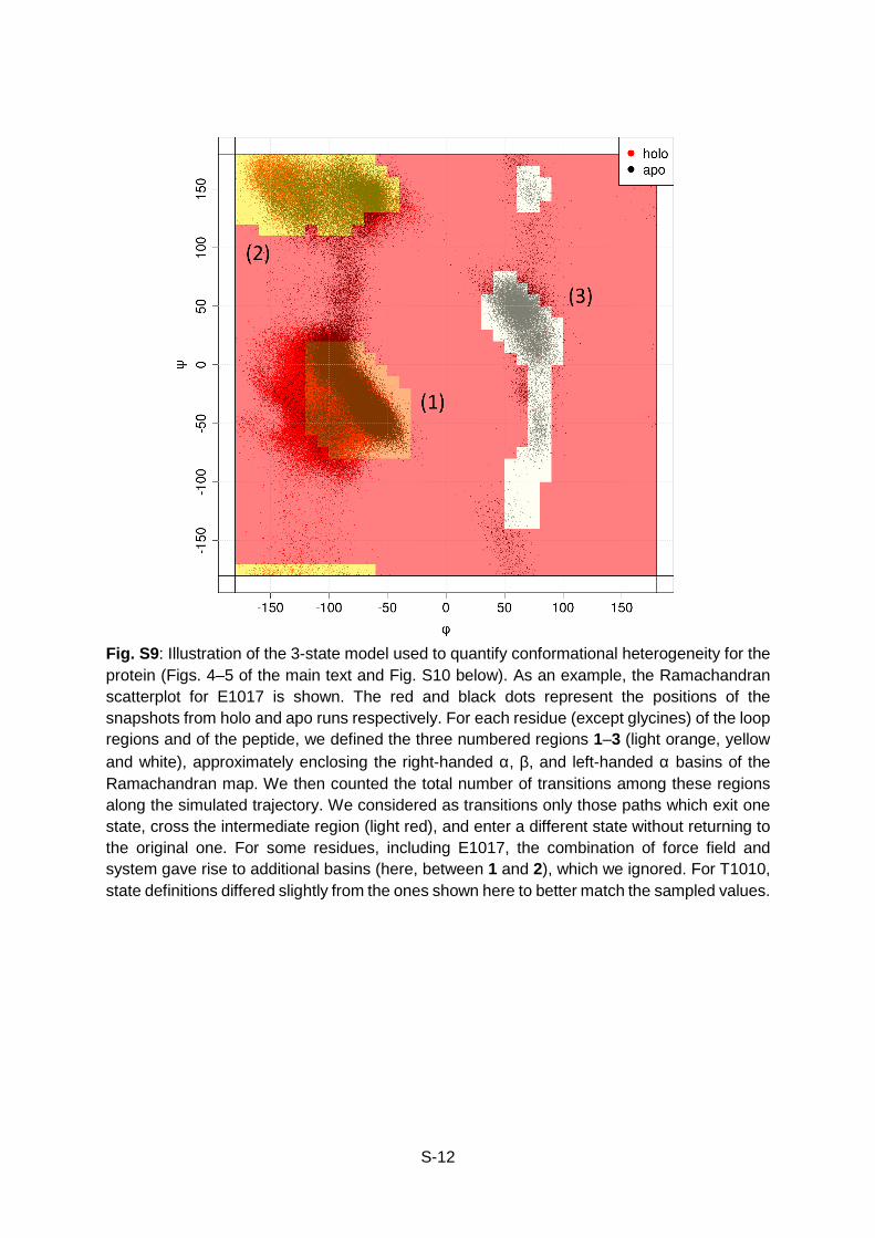
Fig. S9: Illustration of the 3-state model used to quantify conformational heterogeneity for the protein (Figs. 4–5 of the main text and Fig. S10 below). As an example, the Ramachandran scatterplot for E1017 is shown. The red and black dots represent the positions of the snapshots from holo and apo runs respectively. For each residue (except glycines) of the loop regions and of the peptide, we defined the three numbered regions 1–3 (light orange, yellow and white), approximately enclosing the right-handed α, β, and left-handed α basins of the Ramachandran map. We then counted the total number of transitions among these regions along the simulated trajectory. We considered as transitions only those paths which exit one state, cross the intermediate region (light red), and enter a different state without returning to the original one. For some residues, including E1017, the combination of force field and system gave rise to additional basins (here, between 1 and 2), which we ignored. For T1010, state definitions differed slightly from the ones shown here to better match the sampled values.

S-13

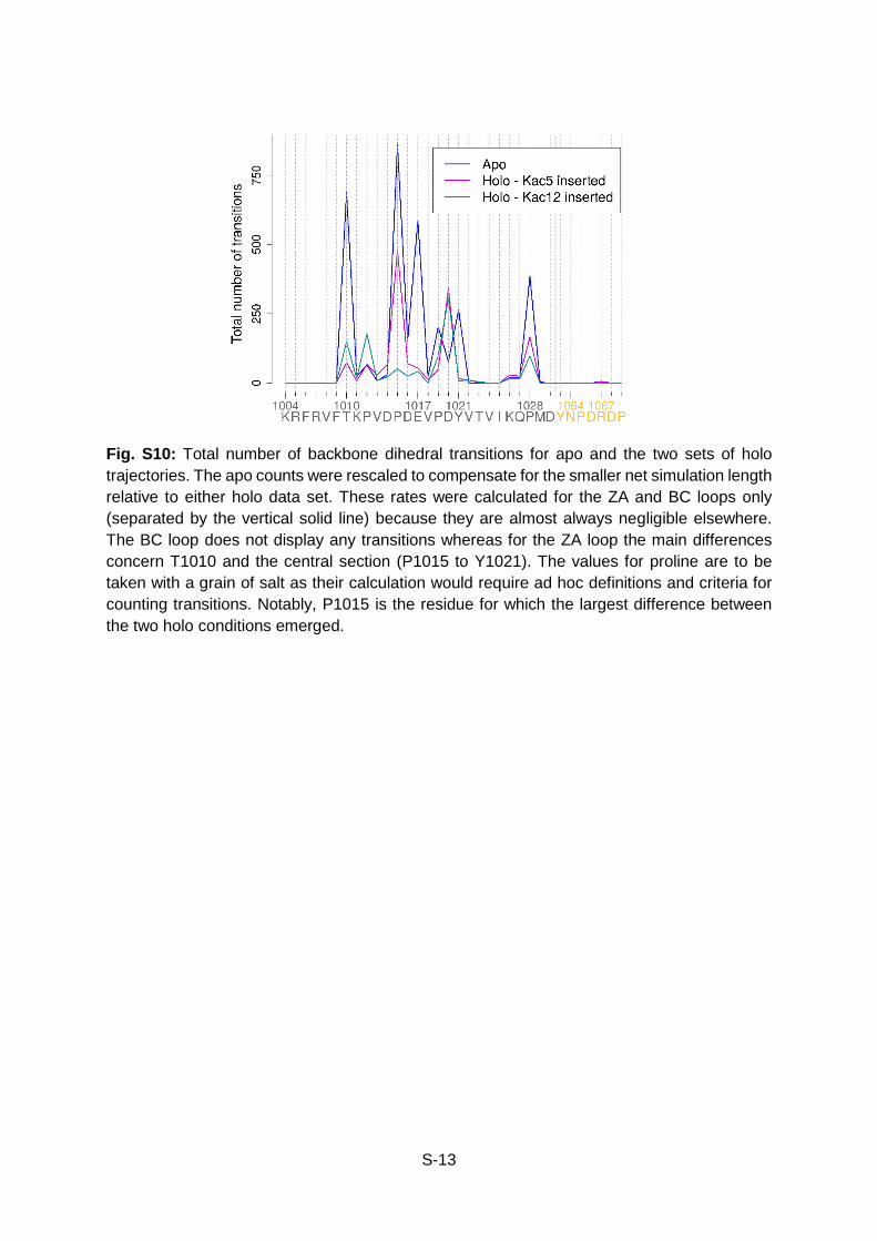
Fig. S10: Total number of backbone dihedral transitions for apo and the two sets of holo trajectories. The apo counts were rescaled to compensate for the smaller net simulation length relative to either holo data set. These rates were calculated for the ZA and BC loops only (separated by the vertical solid line) because they are almost always negligible elsewhere. The BC loop does not display any transitions whereas for the ZA loop the main differences concern T1010 and the central section (P1015 to Y1021). The values for proline are to be taken with a grain of salt as their calculation would require ad hoc definitions and criteria for counting transitions. Notably, P1015 is the residue for which the largest difference between the two holo conditions emerged.

S-14

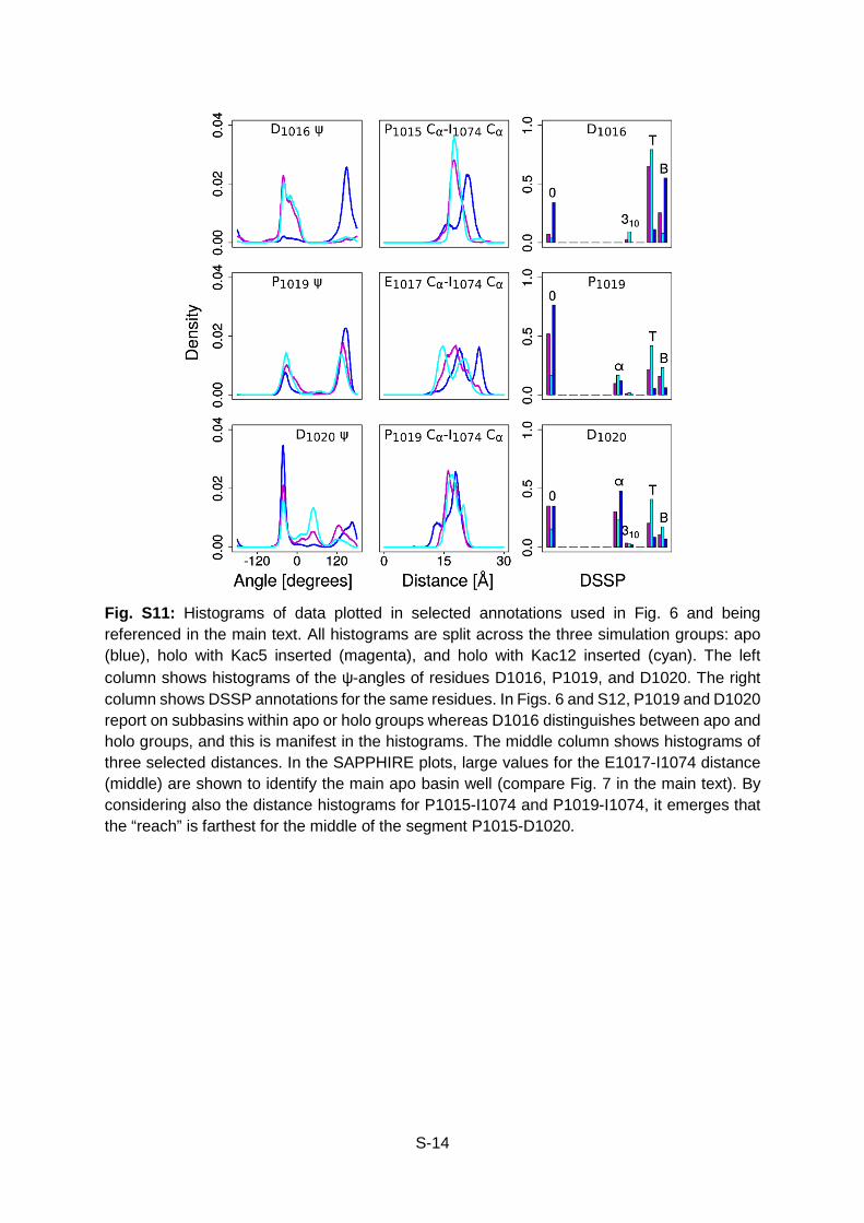
Fig. S11: Histograms of data plotted in selected annotations used in Fig. 6 and being referenced in the main text. All histograms are split across the three simulation groups: apo (blue), holo with Kac5 inserted (magenta), and holo with Kac12 inserted (cyan). The left column shows histograms of the ψ-angles of residues D1016, P1019, and D1020. The right column shows DSSP annotations for the same residues. In Figs. 6 and S12, P1019 and D1020 report on subbasins within apo or holo groups whereas D1016 distinguishes between apo and holo groups, and this is manifest in the histograms. The middle column shows histograms of three selected distances. In the SAPPHIRE plots, large values for the E1017-I1074 distance (middle) are shown to identify the main apo basin well (compare Fig. 7 in the main text). By considering also the distance histograms for P1015-I1074 and P1019-I1074, it emerges that the “reach” is farthest for the middle of the segment P1015-D1020.

S-15

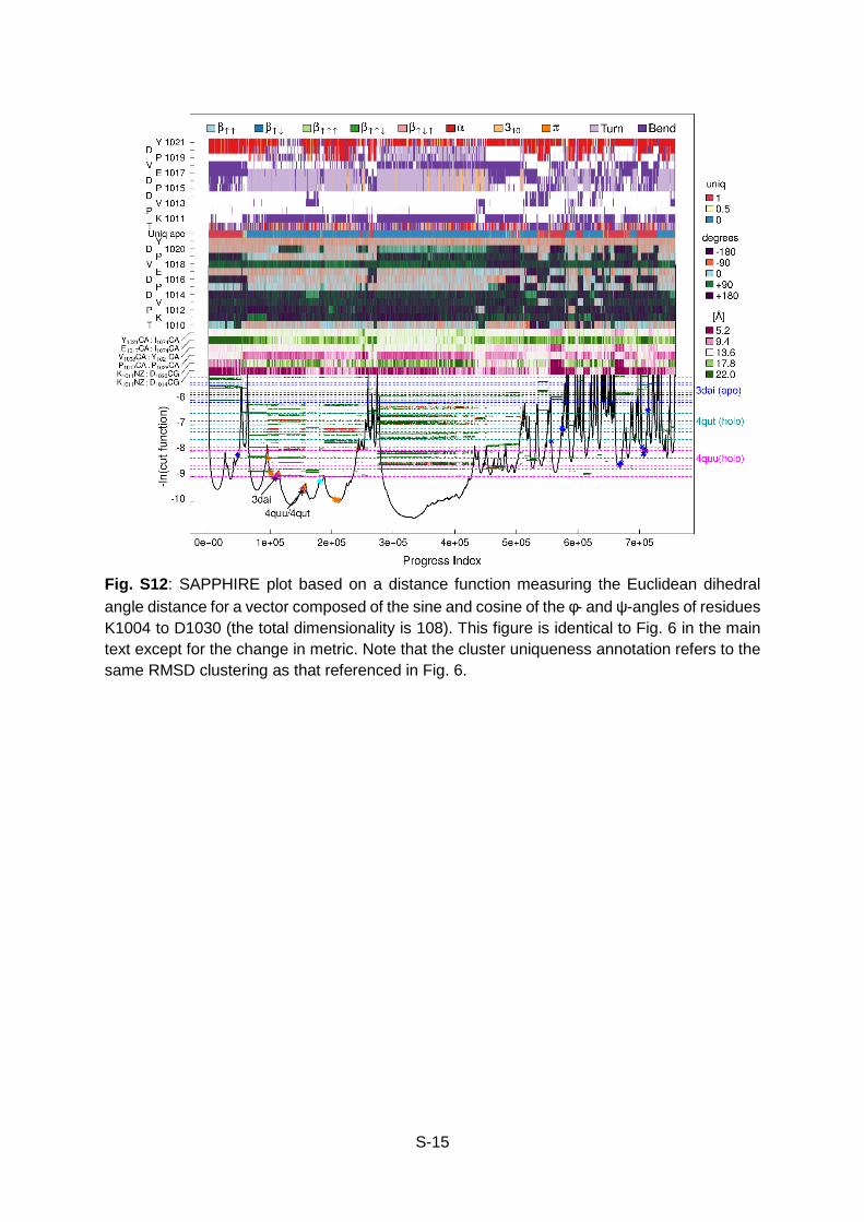
Fig. S12: SAPPHIRE plot based on a distance function measuring the Euclidean dihedral angle distance for a vector composed of the sine and cosine of the φ- and ψ-angles of residues K1004 to D1030 (the total dimensionality is 108). This figure is identical to Fig. 6 in the main text except for the change in metric. Note that the cluster uniqueness annotation refers to the same RMSD clustering as that referenced in Fig. 6.

S-16

SUPPLEMENTAL MOVIE CAPTIONS Movie S1: The movie shows in succession three representations of the relaxed simulation structure of ATAD2A with Kac5 inserted. In the first, the electrostatic potential of just ATAD2A (calculated with APBS (13)) is mapped to the molecular surface of the protein (in UCSF Chimera (14)). The second displays ATAD2A’s van der Waals envelope colored by residue type. The third is a cartoon representation of the H4 histone peptide binding mode with Kac5 inserted. In all representations, a full rotation around the vertical screen axis occurs. For the last rotation, and additional tilt around the horizontal screen axis is shown to show clearly the peptide (some residues are highlighted by sticks). Labels and color legends are incorporated into the movie itself. SUPPLEMENTAL REFERENCES 1. Abraham, M. J., Teemu, M., Roland, S., Szilárd, P., Smith, J. C., Berk, H., and Lindahl,

E. (2015) GROMACS: High performance molecular simulations through multi-level parallelism from laptops to supercomputers. SoftwareX 1-2, 19-25

2. Best, R. B., Zhu, X., Shim, J., Lopes, P. E. M., Mittal, J., Feig, M., and Mackerell, A. D., Jr. (2012) Optimization of the additive CHARMM all-atom protein force field targeting improved sampling of the backbone φ, ψ and side-chain χ(1) and χ(2) dihedral angles. J. Chem. Theory Comput. 8, 3257-3273

3. Durell, S. R., Brooks, B. R., and Ben-Naim, A. (1994) Solvent-induced forces between two hydrophilic groups. J. Phys. Chem. 98, 2198-2202

4. Tironi, I. G., René, S., Smith, P. E., and van Gunsteren, W. F. (1995) A generalized reaction field method for molecular dynamics simulations. J. Chem. Phys. 102, 5451-5459

5. Bussi, G., Donadio, D., and Parrinello, M. (2007) Canonical sampling through velocity rescaling. J. Chem. Phys. 126, 014101

6. Hess, B., Berk, H., Henk, B., Berendsen, H. J. C., and E., J. G. (1997) LINCS: A linear constraint solver for molecular simulations. J. Comput. Chem. 18, 1463-1472

7. Berendsen, H. J. C., Postma, J. P. M., Gunsteren, W. F. v., DiNola, A., and Haak, J. R. (1984) Molecular dynamics with coupling to an external bath. J. Chem. Phys. 81, 3684-3690

8. Vitalis, A., and Pappu, R. V. (2009) ABSINTH: A new continuum solvation model for simulations of polypeptides in aqueous solutions. J. Comput. Chem. 30, 673-699

9. Blöchliger, N., Vitalis, A., and Caflisch, A. (2013) A scalable algorithm to order and annotate continuous observations reveals the metastable states visited by dynamical systems. Comput. Phys. Commun. 184, 2446-2453

10. Vitalis, A., and Caflisch, A. (2012) Efficient Construction of Mesostate Networks from Molecular Dynamics Trajectories. J. Chem. Theory Comput. 8, 1108-1120

11. Kabsch, W., and Sander, C. (1983) Dictionary of protein secondary structure: pattern recognition of hydrogen-bonded and geometrical features. Biopolymers 22, 2577-2637

12. Frishman, D., and Argos, P. (1995) Knowledge-based protein secondary structure assignment. Proteins: Struct. Funct. Bioinform. 23, 566-579

13. Baker, N. A., Sept, D., Joseph, S., Holst, M. J., and McCammon, J. A. (2001) Electrostatics of nanosystems: Application to microtubules and the ribosome. Proc. Natl. Acad. Sci. USA 98, 10037-10041

14. Pettersen, E. F., Goddard, T. D., Huang, C. C., Couch, G. S., Greenblatt, D. M., Meng, E. C., and Ferrin, T. E. (2004) UCSF Chimera—A visualization system for exploratory research and analysis. J. Comput. Chem. 25, 1605-1612