Inverse Kinodynamics:Editing and Constraining Kinematic Approximations of Dynamic Motion

Paul G. Krya, Cyrus Rahgoshaya, Amir Rabbania, Karan Singhb

aSchool of Computer Science, Centre for Intelligent Machines, McGill UniversitybDepartment of Computer Science, University of Toronto

Abstract

We present inverse kinodynamics (IKD), an animator friendly kinematic work flow that both encapsulates short-lived dynamicsand allows precise space-time constraints. Kinodynamics (KD), defines the system state at any given time as the result of a kinematicstate in the recent past, physically simulated over a short time window to the present. KD is a well suited kinematic approximationto animated characters and other dynamic systems with dominant kinematic motion and short-lived dynamics. Given a dynamicsystem, we first choose an appropriate kinodynamic window size based on accelerations in the kinematic trajectory and the physicalproperties of the system. We then present an inverse kinodynamics (IKD) algorithm, where a kinodynamic system can preciselyattain a set of animator constraints at specified times. Our approach solves the IKD problem iteratively, and is able to handle fullpose or end effector constraints at both position and velocity level, as well as multiple constraints in close temporal proximity. Ourapproach can also be used to solve position and velocity constraints on passive systems attached to kinematically driven bodies. Wedescribe both manual and automatic procedures for selecting the kinodynamic window size necessary to approximate the dynamictrajectory to a given accuracy. We demonstrate the convergence properties of our IKD approach, and give details of a typical workflow example that an animator would use to create an animation with our system. We show IKD to be a compelling approach to thedirect kinematic control of character, with secondary dynamics via examples of skeletal dynamics and facial animation.

Keywords: inverse kinematics, secondary dynamics, key framing

1. Introduction1

Physical simulation is now a robust and common approach2

to recreating reality in virtual worlds and is almost universally3

used in the animation of natural phenomena, ballistic objects,4

and character accessories like clothing and hair. Despite these5

strides, the animation of primary characters continues to be6

dominated by the kinematic techniques of motion capture and7

above all traditional keyframing. Two aspects of a primary8

character in particular, skeletal and facial motion, are often la-9

boriously animated using kinematics.10

We note from conversations with about half a dozen mas-11

ter animators that there are perhaps three chief reasons for this.12

First, kinematics, unencumbered by physics, provides the finest13

level of control necessary for animators to breathe life and per-14

sonality into their characters. Second, this control is direct and15

history-free, in that the authored state of the character, set at any16

point in time, is precisely observed upon playback and its im-17

pact on the animation is localized to a neighborhood around that18

time. Third, animator interaction with the time-line is WYSI-19

WYG (what you see is what you get), allowing them to scrub to20

various points in time and instantly observe the character state21

without having to playback the entire animation.22

The same animators expressed the utility and importance of23

secondary dynamics overlaid on primarily kinematic character24

motion to enhance the visceral feel of their characters. Various25

approaches to such secondary dynamics have been proposed26

in research literature [1, 2, 3], some of which are available in27

commercial animation software. Overlaid dynamics, unfortu-28

nately compromise the second and third reasons animators rely29

on pure kinematic control.30

A kinematic solution incorporating secondary dynamics31

called kinodynamic skinning [4] was suggested in the context32

of volume preserving skin deformations. With this approach, a33

kinodynamic state at any time is defined as a kinematic state in34

the recent past, physically simulated forward to the given time.35

In this paper we develop this idea of kinodynamics (KD) as36

a history-free kinematic technique that can incorporate short-37

lived dynamic behavior. Note that the above usage of the term38

“kinodynamic”, while similar in spirit, is distinct from its use in39

the context of robot motion planning where it addresses plan-40

ning problems where velocity and acceleration bounds must be41

satisfied [5].42

The KD window size determines how far into the recent past43

we start a physical simulation in order to compute a KD state.44

We must formulate an appropriate KD window size for a given45

kinematic motion and physical parameters: both long enough46

to ensure a temporally coherent KD trajectory that captures the47

nuances of system dynamics, and short enough for interactive48

WYSIWYG computation and temporal localization of the in-49

fluence of animation edits on system state. Many goal directed50

actions such as grasping, reaching, stepping, gesticulating, and51

even speaking, however, involve spatial relationships between52

the character and its environment, that are best specified di-53

Preprint submitted to Computers & Graphics August 30, 2012

rectly, as targets states that the character (or parts of the char-54

acter) must observe at given times. Techniques such as inverse55

kinematics (IK) and space time optimization algorithmically in-56

fer the remaining system states and animation parameters from57

these animator specified spatio-temporal targets. However, IK58

does not give the secondary dynamics, and space time opti-59

mization is typically computationally expensive. Analogous to60

these techniques, we develop an inverse kinodynamics (IKD)61

algorithm allowing animators to prescribe position and velocity62

constraints at specific points in time within a KD setting.63

Kinodynamics is an interesting approach for interactive64

character animation, where animators can continue to leverage65

a direct history-free kinematic work flow, coupled with the ben-66

efits of arbitrary physically simulated secondary dynamics. The67

problem that we are solving is the inverse kinodynamics prob-68

lem, and our solution allows an animator to easily edit kino-69

dynamic trajectories such that desired constraints can be met.70

Specifically, the contributions of this paper are71

• an iterative inverse kynodynamics (IKD) solver with fast72

convergence properties;73

• details on how to implement our IKD solver for a wide74

range of scenarios: constraints on full poses or hands and75

feet in character animation, position and velocity con-76

straints, multiple overlapping constraints, and constraints77

on passive deformable objects and in facial animation;78

• an automatic method for selecting kinodynamic time79

windows from the physical parameters of the system and80

acceleration bounds on the kinematic trajectory.81

We also discuss limitations, timings, convergence rates, and we82

describe a typical work flow example that an animator would83

use to create an animation with our system.84

2. Related work85

Secondary dynamics provides a significant amount of visual86

realism in kinematically driven animations and is an important87

technique for animators. In the case of tissue deformations pro-88

duced by the motion of an underlying skeleton, various methods89

can be used to produce this motion through simulation or using90

precomputation [1, 2, 3]. With respect to secondary dynam-91

ics of skeletal motion, it has similarly been demonstrated that92

tension and relaxation of the skeletal animation can be altered93

through physically based simulation [6]. These techniques pro-94

vide an important richness to an animation; while the style of95

the results are controllable by adjusting the elastic parameters96

or gains of controllers used for tracking, precise control of the97

motion itself to satisfy given constraints or key frames is typi-98

cally left as a separate problem.99

In constrast to the simulations that provide secondary dy-100

namics, it is the direct local control and WYSIWYG interface101

provided by forward and inverse kinematics techniques that an-102

imators primarily use in the creation of character animation.103

As a result, there has been a vast amount of research on inverse104

kinematics over the years, for instance, combining direct and in-105

verse control during editing [7], using nonlinear programming106

[8], using priority levels to manage conflicting constraints [9],107

or alternatively, singularity-robust inverse computations [10] or108

damped least squares [11]. In this work our focus is on a prob-109

lem similar to inverse kinematics, but in the new setting of kin-110

odynamics. We leave the issue of solving inverse kinodynamics111

in the presence of conflicting constraints for future work.112

The rest of the related work can be categorized into two113

groups. First, there are approaches which try to control a physi-114

cally based simulation to have it meet some desired constraints.115

Second, there are approaches which use kinematic editing tech-116

niques to produce animations that meet desired constraints and117

exhibit physically plausibility.118

Controlling physically based simulations is a difficult prob-119

lem. There has been a significant amount of work in this area120

on controlling rigid bodies [12, 13], fluids [14, 15], and cloth121

[16]. Other recent successes on controlling physically based122

animation use gentle forces to guide an animation along a de-123

sired trajectory, accurately achieving desired states, but also124

allowing physical responses to perturbations [17]. Physically125

based articulated character control has received a vast amount126

of interest. Building on the seminal work of locomotion con-127

trol [18], it is now possible to have, for instance, animation128

of physically based motions that respond naturally to perturba-129

tions [19, 20, 21], maintain balance during locomotion [22, 23],130

and editable animations of dynamic manipulations that respect131

the dynamic interactions between characters and objects [24].132

Our work is very different from these approaches, and is in-133

stead more closely related to work by Allen et al. [25], which134

changes PD control parameters to produce skeletal animations135

that interpolate key-frames at specific times. In our work, how-136

ever, we keep the control parameters fixed and alter the kine-137

matic trajectory.138

Jain and Liu [26] show a method for interactively editing139

interaction between physically based objects and a human. In140

this work, it is the motion of the dynamic environment which is141

edited through kinematic changes of a captured human motion.142

In comparison, we focus on altering and editing a kinodynamic143

motion with different styles (tension and relaxation) and dif-144

ferent constraints. Directly related to the problem of authoring145

motion, physically correct motion can be achieved by solving146

optimizations with space-time constraints [27]. Also relevant147

is work that uses analytic PD control trajectories for compliant148

interpolation [28], and work on generating physically plausible149

motion from infeasible reference motion using a dynamics filter150

[29].151

In contrast to the work on controlling fully dynamic simu-152

lations, we are addressing a simplified problem due to the finite153

time window involved in simulating the state at a given time in154

a kinodynamic trajectory. This leads to benefits in the context155

of animation authoring, and allows for a straightforward solu-156

tion to the inverse kinodynamic problem that we present in this157

paper. We use correction curves with a limited temporal width158

to solve the IKD problem. In a scenario with many constraints159

at different times, the correction resembles a smooth displace-160

ment function, such as the B-splines that are commonly used161

in solving spacetime constraint problems (for instance, in the162

motion editing work of Gleicher [30]). An important difference163

2

is that our displacements are applied on the reference kinematic164

trajectory, thus the final motion is the product of a physical sim-165

ulation as opposed to a displaced motion that satisfies physical166

constraints. In a different approach, with similar objectives to167

our own work, Kass and Anderson [31] propose a method for168

including physically based secondary dynamics in a key frame169

style editing environment through interactive solutions of space170

time optimization problems. They focus on linear or linearized171

space-time constraints problems, while our work, in contrast,172

looks primarily at non-linear problems such as skeletal anima-173

tion.174

Specifically with respect to inverse kinematics, Boulic175

et al. [32] include a control of the center of mass that gener-176

ates character postures with improved plausibility by satisfy-177

ing static balance constraints. Also within a purely kinematic178

setting, Coleman et al. [33] create handles to edit motion ex-179

trema of different joints clustered in time. The visual impact180

of secondary dynamics is often captured in these temporal re-181

lationships. Such an approach can, however, only exaggerate182

or diminish a dynamic effect already present in the motion and183

cannot introduce new forces and dynamic behaviors that the184

mixing of kinematics and dynamics allows.185

Mixing kinematics and dynamics to get the best of both186

has promise for authoring motion in real time. For instance,187

Nguyen et al. [34] blend kinematic animation and dynamic an-188

imation via a set of forces which act like puppet strings to189

pull the character back to the kinematic trajectory. Also of190

note is work on editing kinematic motion through momen-191

tum and force [35], or with biomechanically inspired con-192

straints [36]. While these different approaches use dynamic193

principles to control accelerations and velocity, they deal with194

dynamic systems which are not necessarily short lived, and195

these approaches do not share our objective of a scrubbing in-196

terface for animation editing which computes states largely in a197

history free manner.198

3. Overview199

In this section, we provide an overview of our approach.200

The animation is principally driven by a kinematic trajectory201

xK(t), typically authored and edited using traditional keyframe202

and motion capture techniques. The kinodynamic trajectory of203

the system xKD(t) at a time t is the result of a physical simu-204

lation run over a time window δ starting from an initial posi-205

tion xK(t − δ ) and velocity xK(t − δ ). The simulation uses a206

PD (Proportional-Derivative) controller to follow the kinematic207

trajectory, so the xK(t) can be thought of as the target or desired208

trajectory. The PD controller applies forces to the system that209

are proportional to the difference between the set point xK and210

the process variable x. We also apply viscous damping, thus211

the forces can be written as Kp(xK −x)−Kd x, where the gain212

Kp can be seen as modeling tension and relaxation, while Kd213

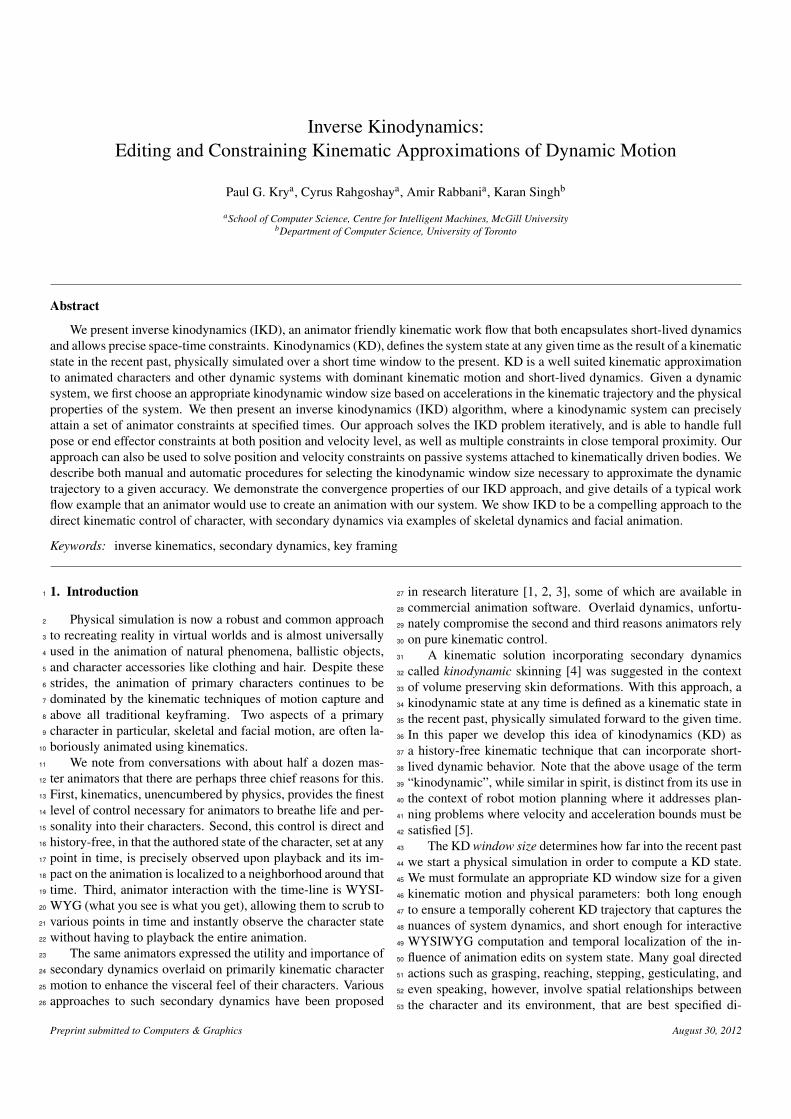
controls damping. Figure 1 shows an example of KD trajecto-214

ries computed with different time windows, which can also be215

seen in the supplementary video. Note how the history-free KD216

trajectories capture the visual behavior of the actual dynamics217

over a range of window sizes.218

Figure 1: KD trajectories for the green ball: Kinematically the green ball isrigidly connected to the keyframed red ball, with spring dynamics overlaid.A number of frames of the KD trajectory (δ = 15) are shown, with the fulldynamics solution for the green ball overlaid in blue (top). KD trajectories with3 window sizes are shown in relation to a full dynamics solution (bottom).

We will have kinodynamic states which deviate from the219

kinematic trajectory because we are using a simulation with220

control forces to generate the KD trajectory. This is desirable221

because we want to include the effects of secondary dynamics222

in the animation. However, there may be specific times in the223

animation where we need constraints to be met.224

Suppose target pose xi must be produced at time ti. This225

target state could be a pose in the original kinematic trajectory,226

or something different. If the pose belongs to the original kine-227

matic trajectory, a simple solution would be to stiffen the PD228

control in the vicinity of the desired pose so that it is tracked229

precisely. Note, however, that stiffness is an inherent attribute230

of the motion’s secondary dynamics under animator control and231

altering it to interpolate a target pose imbues the animation with232

a different style. Instead, we iteratively compute a modification233

to the kinematic trajectory which results in a KD state that sat-234

isfies the constraint.235

Example trajectories and an IKD modification are illus-236

trated in Figure 2, where a red kinodynamic trajectory follows237

a green kinematic trajectory (suppose it is lower due to grav-238

ity). At left we can see an illustration of how the time window239

for computing kinodynamic state must be long enough for any240

impulse (smaller than a given maximum) to come sufficiently241

close to rest that it can not be perceived (for instance, based on242

screen pixels or a percentage of the object size). At right in243

the figure we can see a dotted green kinematic trajectory with244

an added bell shape correction, which produces the dotted red245

kinodynamic trajectory satisfying the constraint at time ti. This246

smooth modification of the kinematic trajectory is the approach247

we use to solve the IKD problem. We use a Gaussian shaped248

correction curve in this work, but a variety of artist designed249

curves that define a smooth ease-in ease-out correction can be250

used, as described in Section 6.251

3.1. Inverse kinodynamics252

Here we formalize our core approach to solving the IKDproblem. Let SimulateKD(xK , ti, δ ) be the procedure for com-puting xKDi, the KD state at ti for kinematic trajectory xK . We

3

Time

x

xKD(t) kinematic

xK(t-d)

d

ti

kinodynamic

simulated trajectoryD x

d d

Posi

tion

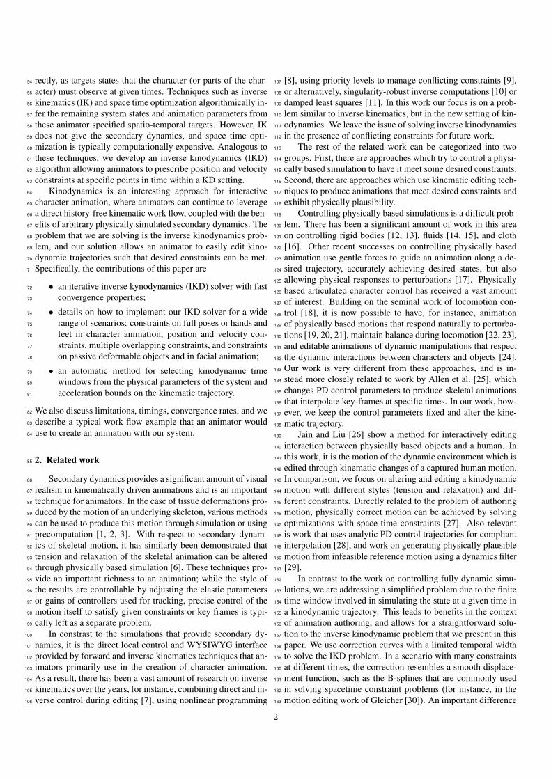
Figure 2: An illustration of how we modify a kinematic trajectory to create akinodynamic trajectory that satisfies the constraint that the original kinematicstate be produced at time ti.

first compute the IKD error in meeting the target as

ei = xi−xKDi, (1)

and from this we form bell shaped correction curves eiφi(t)that we add to kinematic trajectory (note that ei is a vectorof same dimension as the state, and each coordinate of thestate will have a bell shaped correction of a different magni-tude). The bell shaped basis function φi(t) provides a localcorrection, has its peak value of 1 at ti, and can be definedas a low degree polynomial or Gaussian. More importantly,it has a local support (a small temporal width, σ ) which is se-lected by the artist. Conceptually, this IKD error correction in-troduces an additional spring force proportional to eiφi(t) in asmall temporal neighborhood around ti. This correction willnot be sufficient, however, and our modified KD state xKDi =SimulateKD(xK + eiφi, ti,δ ) will not meet the constraint. Thisis because the correction did not take into account the dynamicsof the system, but we can fix this by boosting the correction toaccount for the dynamics, assuming that the system dynamicsare approximately locally linear. Letting di = xKDi− xKDi, weproject the error onto this initial correction result to computethe scaled correction

f(t) = ∆xiφi(t), (2)

where ∆xi =(ei ·di/||di||2

)ei. Figure 3 shows a 2D illustration253

of how this scaling encourages good progress toward the tar-254

get on each iteration. Without this linear prediction step, the255

convergence is significantly slower.256

Using xK + f, the process is repeated, until the system stateconverges to within a numerical threshold of xi at ti. That is, wefind the new kinodynamic state at ti, compute the error ei, themodified kinodynamic state using xK + f+ eiφi, the correctionresult di, and finally an update to the correction function

∆xi← ∆xi +(ei ·di/||di||2

)ei. (3)

4. KD animation and IKD scenarios257

In this paper, we look at a number of scenarios that can258

largely be described as either pose constraints (as described259

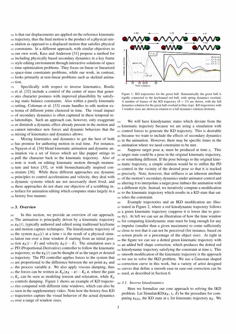
Figure 3: An illustration for a 2D state of two steps of the IKD iteration fora constraint at time ti. At bottom left, xKDi0 is the initial KD state at time ti,which is far from target xi. A correction based on e results in the modified KDstate xKDi1 , which does not take into account the system dynamics. We projectthe error onto di = xKDi1 − xKDi0 to determine a scaling of the correction thatwould produce a KD state as close as possible to xi assuming linear systemdynamics. Using the scaled correction (Equation 3), we produce the new KDstate xKDi1 , and repeat the process until ||e|| falls below a threshold.

above) or end effector constraints (Section 4.1). For instance,260

we may want a kinodynamic skeletal animation of a dance to261

produce some key poses, or a kinodynamic skeletal animation262

of a punch that actually hits the desired target at a specific time.263

Alternatively, another scenario which is important to consider264

is the case where we drive a deformable mesh animation to fol-265

low a target mesh animation. In contrast to joint angles, this266

case involves a state vector formed by the Cartesian position of267

vertices in the mesh. In Section 4.5, we show how this approach268

can be used for facial animation.269

We note that the blending of the correction can be done in a270

number of ways. If we only have one position constraint to sat-271

isfy in the entire animation, then it would be possible to naively272

apply a constant offset to the kinematic trajectory in order to273

meet the constraint at time ti. Typically we will have several274

constraints at different times, so we only make a local edit to275

the desired trajectory (see Section 4.2). Any of a number of276

smoothly shaped curves with compact support will serve this277

purpose, as discussed in Section 6. The shape and width of the278

correction basis functions are an important artist control, much279

like setting ease-in ease-out properties in a key frame anima-280

tion.281

4.1. Skeletal animation end effector IKD282

In the case of an articulated character, the state x is a set of283

joint angles, and the simulation uses a PD controller to follow284

the kinematic trajectory. The gains of the controller set the level285

of tension or relaxation of the character [6].286

When editing a skeletal motion, we may wish to set con-287

straints on the entire pose, as described above, but it is also288

important that we are able to constrain only part of the state at289

4

the time of a contact event, for instance, a point on a hand or290

foot (we will call such points end effectors). Suppose the end291

effector position of an articulated character is given by p(x),292

and that it must reach position pi at time ti. In this case, we293

have the constraint p(xKDi) = pi, and we use an inverse kine-294

matics solution to map the end effector error to an error in the295

state.296

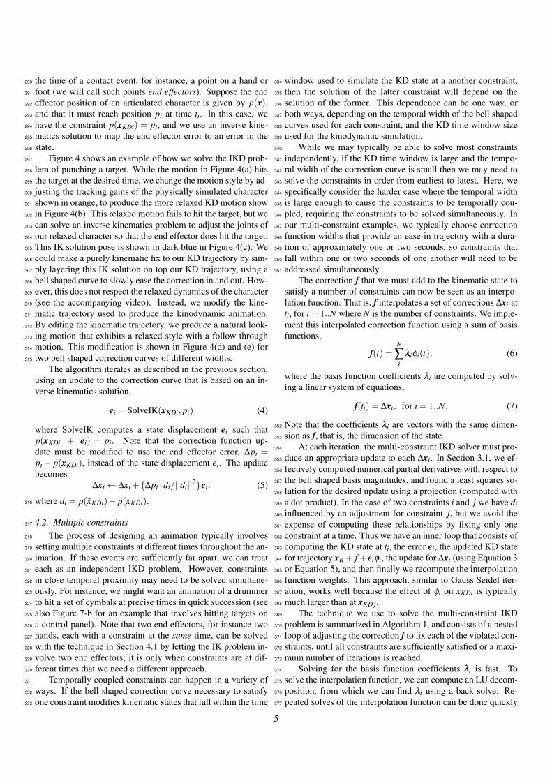
Figure 4 shows an example of how we solve the IKD prob-297

lem of punching a target. While the motion in Figure 4(a) hits298

the target at the desired time, we change the motion style by ad-299

justing the tracking gains of the physically simulated character300

shown in orange, to produce the more relaxed KD motion show301

in Figure 4(b). This relaxed motion fails to hit the target, but we302

can solve an inverse kinematics problem to adjust the joints of303

our relaxed character so that the end effector does hit the target.304

This IK solution pose is shown in dark blue in Figure 4(c). We305

could make a purely kinematic fix to our KD trajectory by sim-306

ply layering this IK solution on top our KD trajectory, using a307

bell shaped curve to slowly ease the correction in and out. How-308

ever, this does not respect the relaxed dynamics of the character309

(see the accompanying video). Instead, we modify the kine-310

matic trajectory used to produce the kinodynamic animation.311

By editing the kinematic trajectory, we produce a natural look-312

ing motion that exhibits a relaxed style with a follow through313

motion. This modification is shown in Figure 4(d) and (e) for314

two bell shaped correction curves of different widths.315

The algorithm iterates as described in the previous section,using an update to the correction curve that is based on an in-verse kinematics solution,

ei = SolveIK(xKDi, pi) (4)

where SolveIK computes a state displacement ei such thatp(xKDi + ei) = pi. Note that the correction function up-date must be modified to use the end effector error, ∆pi =pi− p(xKDi), instead of the state displacement ei. The updatebecomes

∆xi← ∆xi +(∆pi ·di/||di||2

)ei. (5)

where di = p(xKDi)− p(xKDi).316

4.2. Multiple constraints317

The process of designing an animation typically involves318

setting multiple constraints at different times throughout the an-319

imation. If these events are sufficiently far apart, we can treat320

each as an independent IKD problem. However, constraints321

in close temporal proximity may need to be solved simultane-322

ously. For instance, we might want an animation of a drummer323

to hit a set of cymbals at precise times in quick succession (see324

also Figure 7-b for an example that involves hitting targets on325

a control panel). Note that two end effectors, for instance two326

hands, each with a constraint at the same time, can be solved327

with the technique in Section 4.1 by letting the IK problem in-328

volve two end effectors; it is only when constraints are at dif-329

ferent times that we need a different approach.330

Temporally coupled constraints can happen in a variety of331

ways. If the bell shaped correction curve necessary to satisfy332

one constraint modifies kinematic states that fall within the time333

window used to simulate the KD state at a another constraint,334

then the solution of the latter constraint will depend on the335

solution of the former. This dependence can be one way, or336

both ways, depending on the temporal width of the bell shaped337

curves used for each constraint, and the KD time window size338

used for the kinodynamic simulation.339

While we may typically be able to solve most constraints340

independently, if the KD time window is large and the tempo-341

ral width of the correction curve is small then we may need to342

solve the constraints in order from earliest to latest. Here, we343

specifically consider the harder case where the temporal width344

is large enough to cause the constraints to be temporally cou-345

pled, requiring the constraints to be solved simultaneously. In346

our multi-constraint examples, we typically choose correction347

function widths that provide an ease-in trajectory with a dura-348

tion of approximately one or two seconds, so constraints that349

fall within one or two seconds of one another will need to be350

addressed simultaneously.351

The correction f that we must add to the kinematic state tosatisfy a number of constraints can now be seen as an interpo-lation function. That is, f interpolates a set of corrections ∆xi atti, for i = 1..N where N is the number of constraints. We imple-ment this interpolated correction function using a sum of basisfunctions,

f(t) =N

∑i

λiφi(t), (6)

where the basis function coefficients λi are computed by solv-ing a linear system of equations,

f(ti) = ∆xi, for i = 1..N. (7)

Note that the coefficients λi are vectors with the same dimen-352

sion as f, that is, the dimension of the state.353

At each iteration, the multi-constraint IKD solver must pro-354

duce an appropriate update to each ∆xi. In Section 3.1, we ef-355

fectively computed numerical partial derivatives with respect to356

the bell shaped basis magnitudes, and found a least squares so-357

lution for the desired update using a projection (computed with358

a dot product). In the case of two constraints i and j we have di359

influenced by an adjustment for constraint j, but we avoid the360

expense of computing these relationships by fixing only one361

constraint at a time. Thus we have an inner loop that consists of362

computing the KD state at ti, the error ei, the updated KD state363

for trajectory xK + f +eiφi, the update for ∆xi (using Equation 3364

or Equation 5), and then finally we recompute the interpolation365

function weights. This approach, similar to Gauss Seidel iter-366

ation, works well because the effect of φi on xKDi is typically367

much larger than at xKD j.368

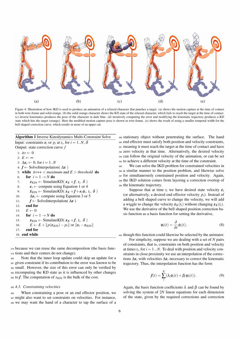
The technique we use to solve the multi-constraint IKD369

problem is summarized in Algorithm 1, and consists of a nested370

loop of adjusting the correction f to fix each of the violated con-371

straints, until all constraints are sufficiently satisfied or a maxi-372

mum number of iterations is reached.373

Solving for the basis function coefficients λi is fast. To374

solve the interpolation function, we can compute an LU decom-375

position, from which we can find λi using a back solve. Re-376

peated solves of the interpolation function can be done quickly377

5

(a) (b) (c) (d) (e)

Figure 4: Illustration of how IKD is used to produce an animation of a relaxed character that punches a target. (a) shows the motion capture at the time of contactin both wire-frame and solid orange. (b) the solid orange character shows the KD state of the relaxed character, which fails to reach the target at the time of contact.(c) inverse kinematics produces the pose of the character in dark blue. (d) iteratively computing the error and modifying the kinematic trajectory produces a KDstate which hits the target (orange). Here the modified motion capture pose is shown in wire-frame. (e) shows the result of using a smaller temporal width for thebell shaped correction curve, which results in more of an upper cut.

Algorithm 1 Inverse Kinodynamics Multi-Constraint SolveInput: constraints xi or pi at ti, for i = 1..N, δ

Output: state correction curve f1: itr← 02: E← ∞

3: ∆xi← 0, for i = 1..N4: f← SolveInterpolation( ∆x )5: while itr++ < maximum and E > threshold do6: for i = 1→ N do7: xKDi← SimulateKD( xK + f, ti, δ )8: ei← compute using Equation 1 or 49: xKDi← SimulateKD( xK + f+ eiφi, ti, δ )

10: ∆xi← compute using Equation 3 or 511: f← SolveInterpolation( ∆x )12: end for13: E← 014: for i = 1→ N do15: xKDi← SimulateKD( xK + f, ti, δ )16: E← E +‖p(xKDi)− pi‖ or ‖xi−xKDi‖17: end for18: end while

because we can reuse the same decomposition (the basis func-378

tions and their centers do not change).379

Note that the inner loop update could skip an update for a380

given constraint if its contribution to the error was known to be381

small. However, the size of this error can only be verified by382

recomputing the KD state as it is influenced by other changes383

to f. The computation of xKDi is the bulk of the cost.384

4.3. Constraining velocities385

When constraining a pose or an end effector position, we386

might also want to set constraints on velocities. For instance,387

we may want the hand of a character to tap the surface of a388

stationary object without penetrating the surface. The hand389

end effector must satisfy both position and velocity constraints,390

meaning it must reach the target at the time of contact and have391

zero velocity at that time. Alternatively, the desired velocity392

can follow the original velocity of the animation, or can be set393

to achieve a different velocity at the time of the constraint.394

We can solve the IKD problem for constrained velocities in395

a similar manner to the position problem, and likewise solve396

for simultaneously constrained position and velocity. Again,397

the IKD solution comes from layering a correction overtop of398

the kinematic trajectory.399

Suppose that at time ti we have desired state velocity xi(or alternatively, a desired end effector velocity pi). Instead ofadding a bell shaped curve to change the velocity, we will adda wiggle to change the velocity xK(ti) without changing xK(ti).We use the derivative of the bell shaped position correction ba-sis function as a basis function for setting the derivative,

ψi(t) =∂

∂ tφi(t), (8)

though this function could likewise be selected by the animator.400

For simplicity, suppose we are dealing with a set of N pairsof constraints, that is, constraints on both position and velocityat times ti, for i = 1...N. To deal with position and velocity con-straints in close proximity we use an interpolation of the correc-tions ∆xi with velocities ∆xi necessary to correct the kinematictrajectory. Thus, the interpolation function has the form

f(t) =N

∑i(λiφi(t)+βiψi(t)). (9)

Again, the basis function coefficients λ and β can be found bysolving the system of 2N linear equations for each dimensionof the state, given by the required corrections and correction

6

velocities:

f(ti) = ∆xi, for i = 1..N, (10)

∂ f(ti)∂ t

= ∆xi, for i = 1..N. (11)

It is important to observe that we update the desired ve-locity correction ∆x j by comparing the desired velocity x withthe velocity of the KD trajectory. The velocity of the dynamicsimulation which produces xKD(t) does not give us this KD ve-locity (it is not the dynamic simulation velocity that we want tocontrol). Instead, we must approximate this KD state velocityfrom successive frames of the KD state,

xKD(ti)≈1h(xKD(ti)−xKD(ti−h)). (12)

We measure the difference to set the velocity error ei, with401

which we compute a new KD state, and ultimately find an up-402

date to the required velocity correction ∆xi, using a computa-403

tion similar to Equation 3.404

In the above example, we are considering a target velocityon the entire state. If instead our constraint is only on the endeffector of a skeleton, then the approach is slightly different. Inthis case, we compute the approximate KD end effector veloc-ity,

pKD(ti)≈1h(p(xKD(ti))− p(xKD(ti−h))). (13)

The difference between this velocity and the artist requestedend effector velocity pi is then mapped to a state error,

ei = J+(pi− pKD(ti)). (14)

where J+ is a pseudoinverse of the end effector Jacobian J =405

∂ p/∂x evaluated at pose xKD(ti). Again, this error is used to406

update the required velocity correction ∆xi, and the process is407

repeated until our IKD algorithm has converged or we reach a408

maximum number of iterations.409

4.4. Passive deformable object IKD410

The previous sections present solutions that deal with con-411

straints on skeletal motion. While this plays an important role412

in character animation, animators may wish to have more con-413

trol over passive deformable objects attached to kinematically414

driven bodies. Controlling secondary dynamics of such defor-415

mations can be tricky since the motion can only be indirectly416

edited by changing the kinematic motion that drives the sec-417

ondary dynamics. Fortunately, the same techniques can be ap-418

plied to solve IKD problems on deformable objects.419

For example, consider the scenario shown in Figure 7-d,420

where a character with a floppy hat must walk through a door421

without the hat hitting any part of the door frame. In this case,422

the hat would hit the top of door frame at time ti. We can use423

IKD to set a constraint that the tip of the hat must be at a po-424

sition just below the door frame at time ti. In our example, the425

hat is a passive elastic system rigidly attached to the head of the426

character, and the character motion is purely kinematic (and it427

must be altered to change the trajectory of the tip of the hat).428

IKD can be used to control the tip of the hat using the skele-429

tal IKD technique described in Section 4.1, with a small adjust-430

ment. At each iteration of the IKD algorithm, we fix the end431

effector position. In this example it is the tip of the hat, based432

on its kinodynamic position at time ti, even though it is not fixed433

with respect to the character’s head. The IKD solution involves434

a change in the character’s posture, allowing the kinodynamic435

position of the tip of the hat to miss the door frame (see the436

accompanying video).437

4.5. Dynamic blend shape IKD438

The IKD problem for passive deformable objects discussed439

in Section 4.4 can be applied to elastic tissue deformation in440

a variety of scenarios. Particularly in the context of facial441

animation, deformation is tediously authored by animators by442

keyframing linearly blend shape targets [37]. Overlaying sec-443

ondary jiggle and other dynamic nuance currently comes at the444

cost of letting dynamics have the “final word” on the anima-445

tion, with no guarantees of hitting certain expressions. IKD al-446

lows one to overlay this desired secondary dynamics in a kine-447

matic setting and further specify critical poses as target shapes448

to be precisely interpolated, independent of the kinematically449

authored blend shape animation. A loosened facial animation450

can also be kept in sync with the environment (like taking a451

puff from a cigarette or sip from a glass) or an audio track by452

adding checkpoints from the kinematic trajectory as IKD tar-453

gets, so the final facial trajectory has a limited deviation from454

the kinematic input. We implement IKD as a deformation that455

tracks control points on a shape using springs and dampers as456

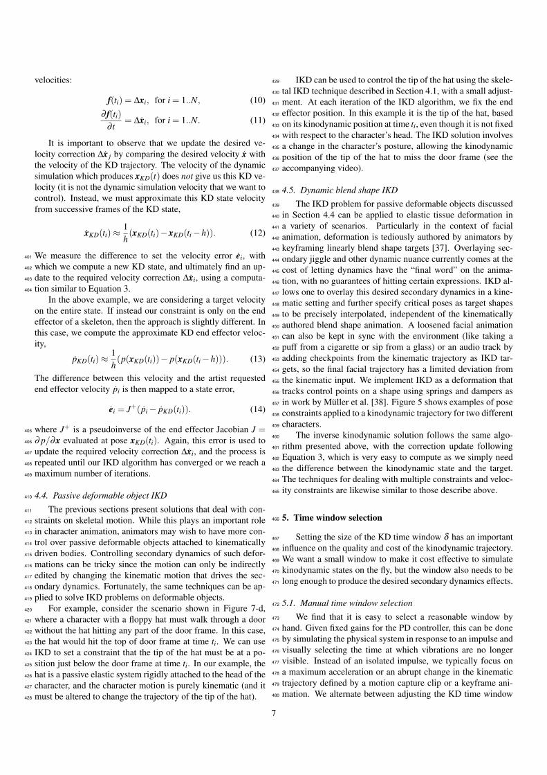
in work by Muller et al. [38]. Figure 5 shows examples of pose457

constraints applied to a kinodynamic trajectory for two different458

characters.459

The inverse kinodynamic solution follows the same algo-460

rithm presented above, with the correction update following461

Equation 3, which is very easy to compute as we simply need462

the difference between the kinodynamic state and the target.463

The techniques for dealing with multiple constraints and veloc-464

ity constraints are likewise similar to those describe above.465

5. Time window selection466

Setting the size of the KD time window δ has an important467

influence on the quality and cost of the kinodynamic trajectory.468

We want a small window to make it cost effective to simulate469

kinodynamic states on the fly, but the window also needs to be470

long enough to produce the desired secondary dynamics effects.471

5.1. Manual time window selection472

We find that it is easy to select a reasonable window by473

hand. Given fixed gains for the PD controller, this can be done474

by simulating the physical system in response to an impulse and475

visually selecting the time at which vibrations are no longer476

visible. Instead of an isolated impulse, we typically focus on477

a maximum acceleration or an abrupt change in the kinematic478

trajectory defined by a motion capture clip or a keyframe ani-479

mation. We alternate between adjusting the KD time window480

7

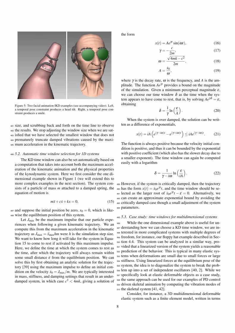
Figure 5: Two facial animation IKD examples (see accompanying video). Left,a temporal pose constraint produces a head tilt. Right, a temporal pose con-straint produces a smile.

size, and scrubbing back and forth on the time line to observe481

the results. We stop adjusting the window size when we are sat-482

isfied that we have selected the smallest window that does not483

prematurely truncate damped vibrations caused by the maxi-484

mum acceleration in the kinematic trajectory.485

5.2. Automatic time window selection for 1D systems486

The KD time window can also be set automatically based ona computation that takes into account both the maximum accel-eration of the kinematic animation and the physical propertiesof the kynodynamic system. Here we first consider the one di-mensional example shown in Figure 1 (we will extend this tomore complex examples in the next section). The system con-sists of a particle of mass m attached to a damped spring, theequation of motion is

mx+ cx+ kx = 0, (15)

and suppose the initial position be zero, x0 = 0, which is like-487

wise the equilibrium position of this system.488

Let Jmax be the maximum impulse that our particle expe-riences when following a given kinematic trajectory. We ancompute this from the maximum acceleration in the kinematictrajectory as Jmax = xmaxhm were h is the simulation step size.We want to know how long it will take for the system in Equa-tion 15 to come to rest if activated by this maximum impulse.Here, we define the time at which the system comes to rest asthe time, after which the trajectory will always remain withinsome small distance ε from the equilibrium position. We cansolve this by first obtaining an analytic solution for the trajec-tory [39] using the maximum impulse to define an initial con-dition on the velocity x0 = Jmax/m. We are typically interestedin mass, stiffness, and damping settings that result in an under-damped system, in which case c2 < 4mk, giving a solution of

the form

x(t) = Aeγt sin(ωt), (16)

γ =− c2m

, (17)

ω =

√4mk− c2

2m, (18)

A =x0

ω, (19)

where γ is the decay rate, ω is the frequency, and A is the am-plitude. The function Aeγt provides a bound on the magnitudeof the simulation. Given a minimum perceptual magnitude ε ,we can choose our time window δ as the time when the sys-tem appears to have come to rest, that is, by solving Aeγδ = ε ,obtaining

δ =1γ

ln(

ε

A

). (20)

When the system is over damped, the solution can be writ-ten as a difference of exponentials,

x(t) = iA(

e(γ−iω)t − e(γ+iω)t)≤ iAe(γ−iω)t . (21)

The function is always positive because the velocity initial con-dition is positive, and thus it can be bounded by the exponentialwith positive coefficient (which also has the slower decay due toa smaller exponent). The time window can again be computedeasily with a logarithm

δ =1

γ− iωln(

ε

iA

). (22)

However, if the system is critically damped, then the trajectory489

has the form x(t) = x0eγtt, and the time window should be se-490

lected as the larger root of x0eγtt − ε = 0. Alternatively, we491

can create an approximate exponential bound by avoiding the492

critically damped case though a small adjustment of the system493

parameters.494

5.3. Case study: time windows for multidimensional systems495

While the one dimensional example above is useful for un-496

derstanding how we can choose a KD time window, we are in-497

terested in more complicated systems with multiple degrees of498

freedom, for instance, our floppy hat example described in Sec-499

tion 4.4. This system can be analyzed in a similar way, pro-500

vided that a linearized version of the system yields a reasonable501

prediction of the behavior. This is typical in many elastic sys-502

tems when deformations are small due to small forces or large503

stiffness. Using linearized forces at the equilibrium pose of the504

system, the idea is to diagonalize the system to break the prob-505

lem up into a set of independent oscillators [40, 2]. While we506

specifically look at elastic deformable objects as a case study,507

the same approach can be used for our examples of PD control508

driven skeletal animation by computing the vibration modes of509

the skeletal system [41, 42].510

Consider, for instance, a 3D multidimensional deformableelastic system such as a finite element model, written in terms

8

of N nodal displacements u ∈ R3N , and recall that some nodesof this system are rigidly attached to a frame, or a “bone”, thatis driven by a kinematic animation. Assuming for now that thebone is stationary, the equations of motion can be written as

Mu+Cu+Ku = 0 (23)

where M is the mass matrix, K is the stiffness computed as theforce gradient at the equilibrium pose, and C = (αM +βK) isthe damping matrix that we assume is Rayleigh. The eigenvaluedecomposition of M−1K gives the modal vibration basis matrixU , which provides a change of coordinates u =Uq, and allowsfor the system to be written as a set of independent oscillators,

miqi + ciqi + kiqi = 0. i = 1..n, (24)

where ci = (αmi +βki). With initial conditions q(0) = 0 andq(0) nonzero, the solution in the under-damped case is

qi(t) = Aieγit sin(ωit), (25)

γi =−ci

2mi, (26)

ωi =

√4miki− c2

i

2mi, (27)

Ai =q(0)ωi

. (28)

The exponential term decays at a minimum rate given by α ,511

and higher frequency modes will have faster decays when β is512

nonzero. Because of this, we focus on a maximum activation513

(through an acceleration of the bone) of the lowest frequency514

mode, i = 1, in order to compute the time window. That is, in-515

stead of solving for the smallest δ such that√

uT u < ε for all516

t > δ , we assume that u(t) will approximately equal U1q1(t)517

near our solution because the contribution of all the higher fre-518

quency modes will have long since become insignificant due to519

their much faster decay rates. Note that√

qT1 UT

1 U1q1 = q1 be-520

cause the eigenvector U1 is unit length, thus we solve A1eδγ1 =521

ε for the time window size δ . Because the problem has been522

reduced to one dimension, we can use the same technique as523

in the previous section to solve for the time window in over-524

damped and critically damped cases too.525

This leaves two points to clarify. First, the selection of the526

perceptual threshold ε , and second, the largest activation of this527

lowest mode that will let us specify the initial condition q1(0).528

We use the Euclidean norm to measure displacement from529

the rest pose, and it can be difficult to set the perceptual thresh-530

old because a model can be discretized with different numbers531

of nodes. We account for this by setting the threshold as the532

value where all nodes are displaced 0.1% of the object diameter533

d, or ε = 0.001d√

N.534

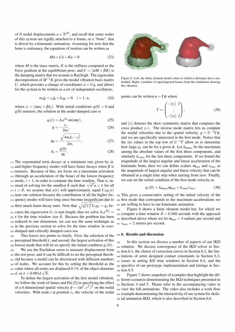
To define the largest activation of the first modal vibration,we follow the work of James and Pai [2] in specifying the effectof a 6 dimensional spatial velocity φ = (ωT ,vT )T on the nodalvelocities. With node i at position ri, the velocity of the nodal

Figure 6: Left, the finite element model cubes in which a christmas hat is em-bedded. Right, a number of superimposed frames from the simulation showingthe vibration.

points can be written u = Γφ where

Γ =

−[r1] I...

−[rN ] I

, (29)

and [ri] denotes the skew symmetric matrix that computes thecross product ri×. The inverse mode matrix lets us computethe modal velocities due to the spatial velocity, q = U−1Γφ ,and we are specifically interested in the first mode. Notice thatthe six values in the top row of U−1Γ allow us to determinehow large q1 can be for a given φ . Let hωmax be the maximumamong the absolute values of the first three components, andsimilarly hvmax for the last three components. If we bound themagnitude of the largest angular and linear acceleration of thekinematic bone, then we can define scalars ωmax and vmax asthe magnitude of largest angular and linear velocity that can beobtained in a single time step when starting from zero. Finally,we can set the initial condition of the first mode velocity as

q1(0) = hωmaxωmax +hvmaxvmax. (30)

This gives a conservative setting of the initial velocity of the535

first mode that corresponds to the maximum accelerations we536

are willing to have in our kinematic animation.537

Figure 6 shows a finite element model hat, for which we538

compute a time window δ = 0.568 seconds with the approach539

described above where we let ωmax = 4 radians per second and540

vmax = 2 meters per second.541

6. Results and discussion542

In this section we discuss a number of aspects of our IKD543

solution. We discuss convergence of the IKD solver in Sec-544

tion 6.1, the choice of correction curves in Section 6.2, the lim-545

itations of artist designed contact constraints in Section 6.3,546

issues in setting KD time windows in Section 6.4, and the547

specifics of our prototype implementation and timings in Sec-548

tion 6.5.549

Figure 7 shows snapshots of examples that highlight the dif-550

ferent scenarios demonstrating the IKD techniques presented in551

Sections 4 and 5. Please refer to the accompanying video to552

view the full animations. The video also includes a work flow553

example demonstrating the interactivity of our system for skele-554

tal animation IKD, which is also described in Section 6.6.555

9

(a) (b) (c) (d) (e)

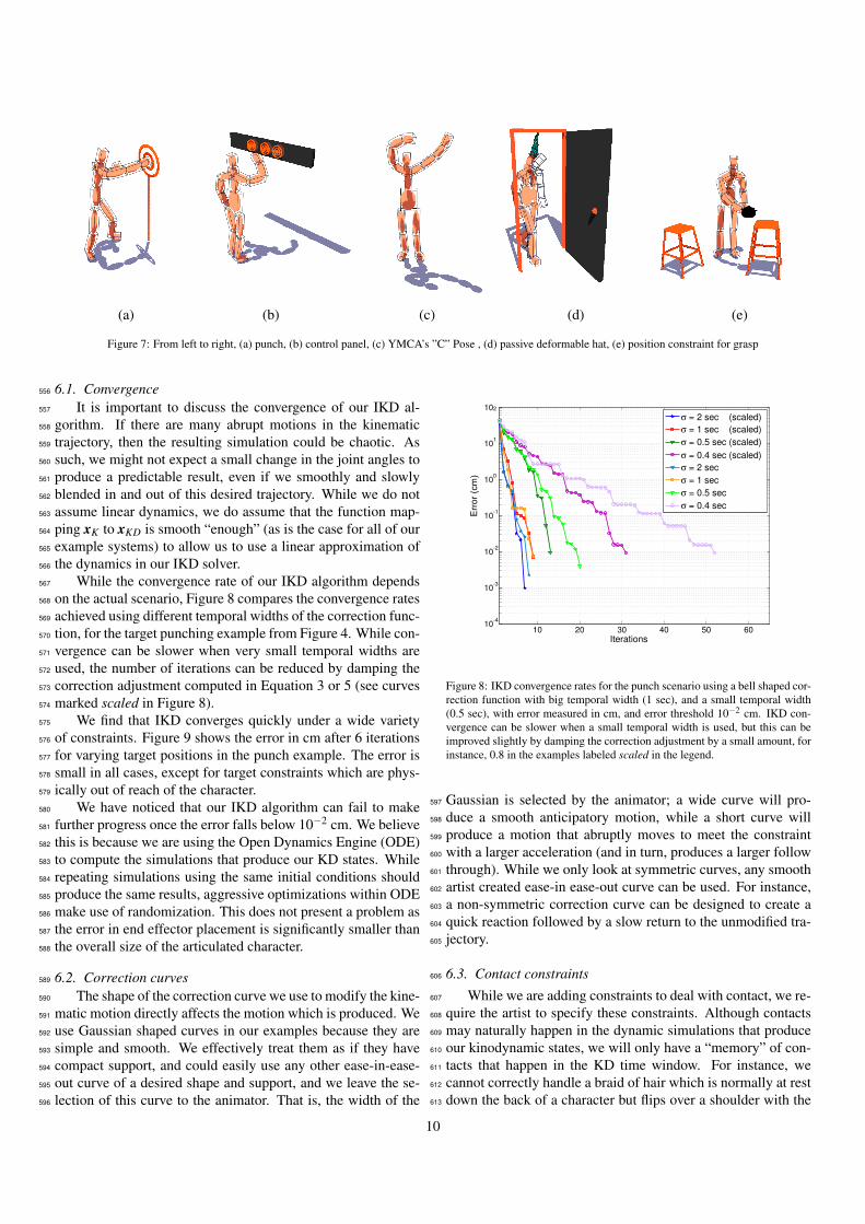
Figure 7: From left to right, (a) punch, (b) control panel, (c) YMCA’s ”C” Pose , (d) passive deformable hat, (e) position constraint for grasp

6.1. Convergence556

It is important to discuss the convergence of our IKD al-557

gorithm. If there are many abrupt motions in the kinematic558

trajectory, then the resulting simulation could be chaotic. As559

such, we might not expect a small change in the joint angles to560

produce a predictable result, even if we smoothly and slowly561

blended in and out of this desired trajectory. While we do not562

assume linear dynamics, we do assume that the function map-563

ping xK to xKD is smooth “enough” (as is the case for all of our564

example systems) to allow us to use a linear approximation of565

the dynamics in our IKD solver.566

While the convergence rate of our IKD algorithm depends567

on the actual scenario, Figure 8 compares the convergence rates568

achieved using different temporal widths of the correction func-569

tion, for the target punching example from Figure 4. While con-570

vergence can be slower when very small temporal widths are571

used, the number of iterations can be reduced by damping the572

correction adjustment computed in Equation 3 or 5 (see curves573

marked scaled in Figure 8).574

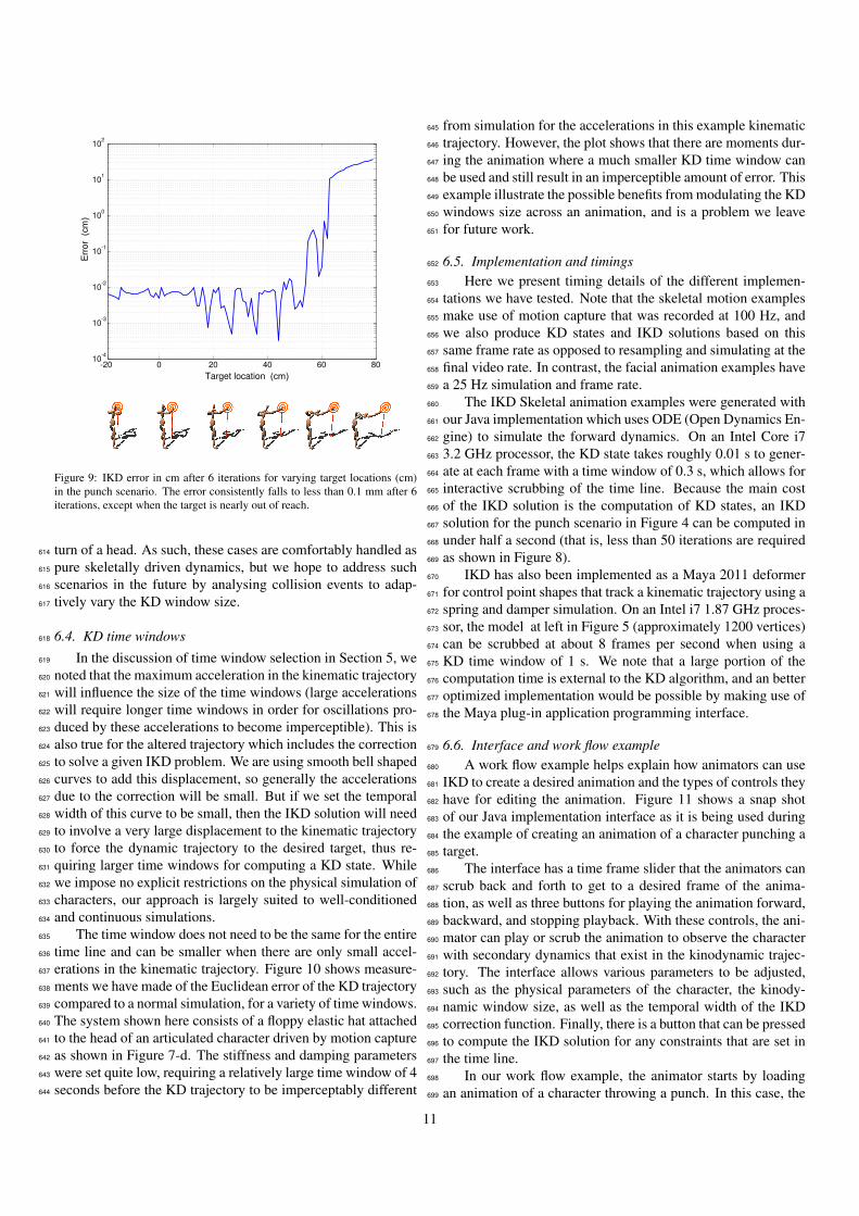
We find that IKD converges quickly under a wide variety575

of constraints. Figure 9 shows the error in cm after 6 iterations576

for varying target positions in the punch example. The error is577

small in all cases, except for target constraints which are phys-578

ically out of reach of the character.579

We have noticed that our IKD algorithm can fail to make580

further progress once the error falls below 10−2 cm. We believe581

this is because we are using the Open Dynamics Engine (ODE)582

to compute the simulations that produce our KD states. While583

repeating simulations using the same initial conditions should584

produce the same results, aggressive optimizations within ODE585

make use of randomization. This does not present a problem as586

the error in end effector placement is significantly smaller than587

the overall size of the articulated character.588

6.2. Correction curves589

The shape of the correction curve we use to modify the kine-590

matic motion directly affects the motion which is produced. We591

use Gaussian shaped curves in our examples because they are592

simple and smooth. We effectively treat them as if they have593

compact support, and could easily use any other ease-in-ease-594

out curve of a desired shape and support, and we leave the se-595

lection of this curve to the animator. That is, the width of the596

10 20 30 40 50 6010

-4

10-3

10-2

10-1

100

101

102

Iterations

Err

or (

cm)

σ = 2 sec (scaled)

σ = 1 sec (scaled)

σ = 0.5 sec (scaled)

σ = 0.4 sec (scaled)

σ = 2 sec

σ = 1 sec

σ = 0.5 sec

σ = 0.4 sec

Figure 8: IKD convergence rates for the punch scenario using a bell shaped cor-rection function with big temporal width (1 sec), and a small temporal width(0.5 sec), with error measured in cm, and error threshold 10−2 cm. IKD con-vergence can be slower when a small temporal width is used, but this can beimproved slightly by damping the correction adjustment by a small amount, forinstance, 0.8 in the examples labeled scaled in the legend.

Gaussian is selected by the animator; a wide curve will pro-597

duce a smooth anticipatory motion, while a short curve will598

produce a motion that abruptly moves to meet the constraint599

with a larger acceleration (and in turn, produces a larger follow600

through). While we only look at symmetric curves, any smooth601

artist created ease-in ease-out curve can be used. For instance,602

a non-symmetric correction curve can be designed to create a603

quick reaction followed by a slow return to the unmodified tra-604

jectory.605

6.3. Contact constraints606

While we are adding constraints to deal with contact, we re-607

quire the artist to specify these constraints. Although contacts608

may naturally happen in the dynamic simulations that produce609

our kinodynamic states, we will only have a “memory” of con-610

tacts that happen in the KD time window. For instance, we611

cannot correctly handle a braid of hair which is normally at rest612

down the back of a character but flips over a shoulder with the613

10

-20 0 20 40 60 8010

-4

10-3

10-2

10-1

100

101

102

Target location (cm)

Err

or

(cm

)

Figure 9: IKD error in cm after 6 iterations for varying target locations (cm)in the punch scenario. The error consistently falls to less than 0.1 mm after 6iterations, except when the target is nearly out of reach.

turn of a head. As such, these cases are comfortably handled as614

pure skeletally driven dynamics, but we hope to address such615

scenarios in the future by analysing collision events to adap-616

tively vary the KD window size.617

6.4. KD time windows618

In the discussion of time window selection in Section 5, we619

noted that the maximum acceleration in the kinematic trajectory620

will influence the size of the time windows (large accelerations621

will require longer time windows in order for oscillations pro-622

duced by these accelerations to become imperceptible). This is623

also true for the altered trajectory which includes the correction624

to solve a given IKD problem. We are using smooth bell shaped625

curves to add this displacement, so generally the accelerations626

due to the correction will be small. But if we set the temporal627

width of this curve to be small, then the IKD solution will need628

to involve a very large displacement to the kinematic trajectory629

to force the dynamic trajectory to the desired target, thus re-630

quiring larger time windows for computing a KD state. While631

we impose no explicit restrictions on the physical simulation of632

characters, our approach is largely suited to well-conditioned633

and continuous simulations.634

The time window does not need to be the same for the entire635

time line and can be smaller when there are only small accel-636

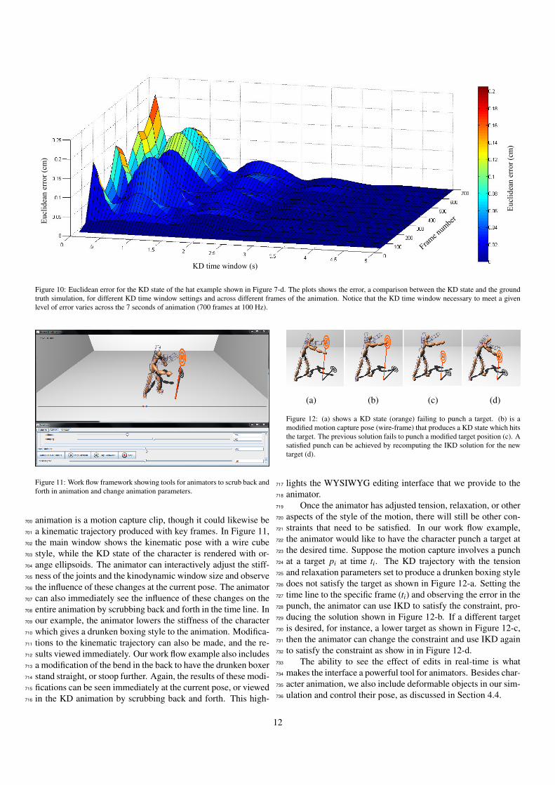
erations in the kinematic trajectory. Figure 10 shows measure-637

ments we have made of the Euclidean error of the KD trajectory638

compared to a normal simulation, for a variety of time windows.639

The system shown here consists of a floppy elastic hat attached640

to the head of an articulated character driven by motion capture641

as shown in Figure 7-d. The stiffness and damping parameters642

were set quite low, requiring a relatively large time window of 4643

seconds before the KD trajectory to be imperceptably different644

from simulation for the accelerations in this example kinematic645

trajectory. However, the plot shows that there are moments dur-646

ing the animation where a much smaller KD time window can647

be used and still result in an imperceptible amount of error. This648

example illustrate the possible benefits from modulating the KD649

windows size across an animation, and is a problem we leave650

for future work.651

6.5. Implementation and timings652

Here we present timing details of the different implemen-653

tations we have tested. Note that the skeletal motion examples654

make use of motion capture that was recorded at 100 Hz, and655

we also produce KD states and IKD solutions based on this656

same frame rate as opposed to resampling and simulating at the657

final video rate. In contrast, the facial animation examples have658

a 25 Hz simulation and frame rate.659

The IKD Skeletal animation examples were generated with660

our Java implementation which uses ODE (Open Dynamics En-661

gine) to simulate the forward dynamics. On an Intel Core i7662

3.2 GHz processor, the KD state takes roughly 0.01 s to gener-663

ate at each frame with a time window of 0.3 s, which allows for664

interactive scrubbing of the time line. Because the main cost665

of the IKD solution is the computation of KD states, an IKD666

solution for the punch scenario in Figure 4 can be computed in667

under half a second (that is, less than 50 iterations are required668

as shown in Figure 8).669

IKD has also been implemented as a Maya 2011 deformer670

for control point shapes that track a kinematic trajectory using a671

spring and damper simulation. On an Intel i7 1.87 GHz proces-672

sor, the model at left in Figure 5 (approximately 1200 vertices)673

can be scrubbed at about 8 frames per second when using a674

KD time window of 1 s. We note that a large portion of the675

computation time is external to the KD algorithm, and an better676

optimized implementation would be possible by making use of677

the Maya plug-in application programming interface.678

6.6. Interface and work flow example679

A work flow example helps explain how animators can use680

IKD to create a desired animation and the types of controls they681

have for editing the animation. Figure 11 shows a snap shot682

of our Java implementation interface as it is being used during683

the example of creating an animation of a character punching a684

target.685

The interface has a time frame slider that the animators can686

scrub back and forth to get to a desired frame of the anima-687

tion, as well as three buttons for playing the animation forward,688

backward, and stopping playback. With these controls, the ani-689

mator can play or scrub the animation to observe the character690

with secondary dynamics that exist in the kinodynamic trajec-691

tory. The interface allows various parameters to be adjusted,692

such as the physical parameters of the character, the kinody-693

namic window size, as well as the temporal width of the IKD694

correction function. Finally, there is a button that can be pressed695

to compute the IKD solution for any constraints that are set in696

the time line.697

In our work flow example, the animator starts by loading698

an animation of a character throwing a punch. In this case, the699

11

Eucl

idea

n er

ror (

cm)

Frame n

umber

Eucl

idea

n er

ror (

cm)

KD time window (s)

Figure 10: Euclidean error for the KD state of the hat example shown in Figure 7-d. The plots shows the error, a comparison between the KD state and the groundtruth simulation, for different KD time window settings and across different frames of the animation. Notice that the KD time window necessary to meet a givenlevel of error varies across the 7 seconds of animation (700 frames at 100 Hz).

Figure 11: Work flow framework showing tools for animators to scrub back andforth in animation and change animation parameters.

animation is a motion capture clip, though it could likewise be700

a kinematic trajectory produced with key frames. In Figure 11,701

the main window shows the kinematic pose with a wire cube702

style, while the KD state of the character is rendered with or-703

ange ellipsoids. The animator can interactively adjust the stiff-704

ness of the joints and the kinodynamic window size and observe705

the influence of these changes at the current pose. The animator706

can also immediately see the influence of these changes on the707

entire animation by scrubbing back and forth in the time line. In708

our example, the animator lowers the stiffness of the character709

which gives a drunken boxing style to the animation. Modifica-710

tions to the kinematic trajectory can also be made, and the re-711

sults viewed immediately. Our work flow example also includes712

a modification of the bend in the back to have the drunken boxer713

stand straight, or stoop further. Again, the results of these modi-714

fications can be seen immediately at the current pose, or viewed715

in the KD animation by scrubbing back and forth. This high-716

(a) (b) (c) (d)

Figure 12: (a) shows a KD state (orange) failing to punch a target. (b) is amodified motion capture pose (wire-frame) that produces a KD state which hitsthe target. The previous solution fails to punch a modified target position (c). Asatisfied punch can be achieved by recomputing the IKD solution for the newtarget (d).

lights the WYSIWYG editing interface that we provide to the717

animator.718

Once the animator has adjusted tension, relaxation, or other719

aspects of the style of the motion, there will still be other con-720

straints that need to be satisfied. In our work flow example,721

the animator would like to have the character punch a target at722

the desired time. Suppose the motion capture involves a punch723

at a target pi at time ti. The KD trajectory with the tension724

and relaxation parameters set to produce a drunken boxing style725

does not satisfy the target as shown in Figure 12-a. Setting the726

time line to the specific frame (ti) and observing the error in the727

punch, the animator can use IKD to satisfy the constraint, pro-728

ducing the solution shown in Figure 12-b. If a different target729

is desired, for instance, a lower target as shown in Figure 12-c,730

then the animator can change the constraint and use IKD again731

to satisfy the constraint as show in in Figure 12-d.732

The ability to see the effect of edits in real-time is what733

makes the interface a powerful tool for animators. Besides char-734

acter animation, we also include deformable objects in our sim-735

ulation and control their pose, as discussed in Section 4.4.736

12

7. Conclusions737

While the IKD interface itself is not a contribution of our738

work, a demonstration of the Maya implementation to a few739

keyframe animators was positively received. From a work flow740

standpoint, the animators felt they would have to consciously741

omit keyframing dynamic nuances but this would be a welcome742

change allowing them focus on the primary motion. For the743

approach to be used in practice they expressed a need for in-744

terface tools that make the addition and management of IKD745

targets user friendly. Our current implementation, while inter-746

active for skeletal animation, is only interactive for face blend747

shapes with around 1000 control vertices. The vectorizable na-748

ture of our algorithm, however, makes it a good candidate for749

a faster GPU implementation. In future work we would like750

to address the coupling of kinodynamic trajectories with fully751

dynamic environments via adaptive kinodynamic window sizes752

that are aware of collision events and other discontinuities in a753

full physical simulation. In summary, we propose the concept754

of Inverse Kinodynamics and present a first algorithm which755

opens up new possibilities for editing traditional keyframe ani-756

mations that are augmented with secondary dynamics.757

Acknowledgments758

This work was supported by NSERC, and GRAND NCE759

Project MOTION, and originated from discussions at the Bel-760

lairs Research Institute during the 2011 Workshop on Computer761

Animation.762

References763

[1] Capell S, Green S, Curless B, Duchamp T, Popovic Z. Interactive764

skeleton-driven dynamic deformations. In: Proceedings of the 29th an-765

nual conference on Computer graphics and interactive techniques. SIG-766

GRAPH ’02. ISBN 1-58113-521-1; 2002, p. 586–93.767

[2] James DL, Pai DK. Dyrt: dynamic response textures for real time de-768

formation simulation with graphics hardware. In: SIGGRAPH. 2002, p.769

582–5.770

[3] Kim J, Pollard NS. Fast simulation of skeleton-driven deformable body771

characters. ACM Trans Graph 2011;30:121:1–121:19.772

[4] Angelidis A, Singh K. Kinodynamic skinning using volume-773

preserving deformations. In: Proceedings of the 2007 ACM SIG-774

GRAPH/Eurographics symposium on Computer animation. SCA ’07;775

Eurographics Association. ISBN 978-1-59593-624-4; 2007, p. 129–40.776

[5] Donald B, Xavier P, Canny J, Reif J. Kinodynamic motion planning. J777

ACM 1993;40:1048–66.778

[6] Neff M, Eugene F. Modeling tension and relaxation for computer anima-779

tion. In: Proceedings of the 2002 ACM SIGGRAPH/Eurographics sym-780

posium on Computer animation. SCA ’02; New York, NY, USA: ACM.781

ISBN 1-58113-573-4; 2002, p. 81–8.782

[7] Boulic R, Thalmann D. Combined direct and inverse kinematic con-783

trol for articulated figure motion editing. Computer Graphics Fo-784

rum 1992;11(4):189–202. doi:10.1111/1467-8659.1140189. URL785

http://dx.doi.org/10.1111/1467-8659.1140189.786

[8] Zhao J, Badler NI. Inverse kinematics positioning using nonlin-787

ear programming for highly articulated figures. ACM Trans Graph788

1994;13(4):313–36.789

[9] Baerlocher P, Boulic R. An inverse kinematics architecture enforcing an790

arbitrary number of strict priority levels. Vis Comput 2004;20(6):402–17.791

[10] Yamane K, Nakamura Y. Natural motion animation through constrain-792

ing and deconstraining at will. IEEE Transactions on Visualization and793

Computer Graphics 2003;9(3):352–60.794

[11] Buss SR, Kim JS. Selectively damped least squares for inverse kinemat-795

ics. Journal of Graphics Tools 2004;10:37–49.796

[12] Popovic J, Seitz SM, Erdmann M, Popovic Z, Witkin A. Interactive ma-797

nipulation of rigid body simulations. In: Proceedings of the 27th an-798

nual conference on Computer graphics and interactive techniques. SIG-799

GRAPH ’00. ISBN 1-58113-208-5; 2000, p. 209–17.800

[13] Popovic J, Seitz SM, Erdmann M. Motion sketching for control of rigid-801

body simulations. ACM Trans Graph 2003;22:1034–54.802

[14] Treuille A, McNamara A, Popovic Z, Stam J. Keyframe control of smoke803

simulations. ACM Trans Graph 2003;22:716–23.804

[15] McNamara A, Treuille A, Popovic Z, Stam J. Fluid control using the805

adjoint method. ACM Trans Graph 2004;23:449–56.806

[16] Wojtan C, Mucha PJ, Turk G. Keyframe control of complex particle807

systems using the adjoint method. In: SCA ’06: Proceedings of the808

2006 ACM SIGGRAPH/Eurographics symposium on Computer anima-809

tion. Eurographics Association. ISBN 3-905673-34-7; 2006, p. 15–23.810

[17] Barbic J, Popovic J. Real-time control of physically based simulations811

using gentle forces. ACM Trans on Graphics (SIGGRAPH Asia 2008)812

2008;27(5):163:1–163:10.813

[18] Raibert MH, Hodgins JK. Animation of dynamic legged locomotion.814

SIGGRAPH Comput Graph 1991;25:349–58.815

[19] Zordan VB, Hodgins JK. Motion capture-driven simulations that hit and816

react. In: Proceedings of the 2002 ACM SIGGRAPH/Eurographics sym-817

posium on Computer animation. SCA ’02; New York, NY, USA: ACM.818

ISBN 1-58113-573-4; 2002, p. 89–96.819

[20] Yin K, Cline MB, Pai DK. Motion perturbation based on simple neuro-820

motor control models. In: Proceedings of the 11th Pacific Conference on821

Computer Graphics and Applications. PG ’03; Washington, DC, USA:822

IEEE Computer Society. ISBN 0-7695-2028-6; 2003, p. 445.823

[21] Zordan VB, Majkowska A, Chiu B, Fast M. Dynamic response for motion824

capture animation. ACM Trans Graph 2005;24:697–701.825

[22] Yin K, Loken K, van de Panne M. Simbicon: simple biped locomotion826

control. ACM Transactions on Graphics 2007;26(3).827

[23] Coros S, Beaudoin P, van de Panne M. Generalized biped walking con-828

trol. In: ACM SIGGRAPH 2010 papers. SIGGRAPH ’10; New York,829

NY, USA: ACM; 2010, p. 1–9.830

[24] Abe Y, Popovic J. Interactive animation of dynamic manipulation. In:831

Proceedings of the 2006 ACM SIGGRAPH/Eurographics symposium on832

Computer animation. SCA ’06; Aire-la-Ville, Switzerland, Switzerland:833

Eurographics Association. ISBN 3-905673-34-7; 2006, p. 195–204.834

[25] Allen BF, Chu D, Shapiro A, Faloutsos P. On the beat!: Timing and ten-835

sion for dynamic characters. In: SCA ’07: Proceedings of the 2007 ACM836

SIGGRAPH/Eurographics symposium on Computer animation. Euro-837

graphics Association. ISBN 978-1-59593-624-4; 2007, p. 239–47.838

[26] Jain S, Liu CK. Interactive synthesis of human-object interaction. In:839

ACM SIGGRAPH/Eurographics Symposium on Computer Animation840

(SCA). ACM. ISBN 978-1-60558-610-6; 2009, p. 47–53.841

[27] Witkin A, Kass M. Spacetime constraints. SIGGRAPH Comput Graph842

1988;22:159–68.843

[28] Allen BF, Neff M, Faloutsos P. Analytic proportional-derivative control844

for precise and compliant motion. In: Robotics and Automation (ICRA),845

2011 IEEE International Conference on. 2011, p. 6039 –44.846

[29] Yamane K, Nakamura Y. Dynamics filter - concept and implementa-847

tion of online motion generator for human figures. IEEE Transactions on848

Robotics and Automation 2003;19(3):421–32.849

[30] Gleicher M. Motion editing with spacetime constraints. In: Proceedings850

of the 1997 symposium on Interactive 3D graphics. I3D ’97; New York,851

NY, USA: ACM; 1997, p. 139–49.852

[31] Kass M, Anderson J. Animating oscillatory motion with overlap: wiggly853

splines. ACM Trans Graph 2008;27:1–8.854

[32] Boulic R, Mas R, Thalmann D. A robust approach for the control855

of the center of mass with inverse kinetics. Computers & graphics856

1996;20(5):693–701.857

[33] Coleman P, Bibliowicz J, Singh K, Gleicher M. Staggered poses:858

a character motion representation for detail-preserving editing of pose859

and coordinated timing. In: Proceedings of the 2008 ACM SIG-860

GRAPH/Eurographics Symposium on Computer Animation. SCA ’08;861

Eurographics Association. ISBN 978-3-905674-10-1; 2008, p. 137–46.862

[34] Nguyen N, Wheatland N, Brown D, Parise B, Liu CK, Zordan V. Perfor-863

mance capture with physical interaction. In: Proceedings of the 2010864

ACM SIGGRAPH/Eurographics Symposium on Computer Animation.865

13

SCA ’10; Eurographics Association; 2010, p. 189–95.866

[35] Sok KW, Yamane K, Lee J, Hodgins J. Editing dynamic human mo-867

tions via momentum and force. In: Proceedings of the 2010 ACM SIG-868

GRAPH/Eurographics Symposium on Computer Animation. SCA ’10;869

Aire-la-Ville, Switzerland, Switzerland: Eurographics Association; 2010,870

p. 11–20.871

[36] Lockwood N, Singh K. Biomechanically-inspired motion path editing.872

In: Proceedings of the 2011 ACM SIGGRAPH/Eurographics Symposium873

on Computer Animation. SCA ’11; New York, NY, USA: ACM. ISBN874

978-1-4503-0923-3; 2011, p. 267–76.875

[37] Pighin F, Hecker J, Lischinski D, Szeliski R, Salesin DH. Synthesiz-876

ing realistic facial expressions from photographs. In: Proceedings of the877

25th annual conference on Computer graphics and interactive techniques.878

SIGGRAPH ’98. ISBN 0-89791-999-8; 1998, p. 75–84.879

[38] Muller M, Heidelberger B, Teschner M, Gross M. Meshless deformations880

based on shape matching. ACM Trans Graph 2005;24:471–8.881

[39] Meirovitch L. Analytical methods in vibrations. Macmillan series in882

advanced mathematics and theoretical physics; Macmillan; 1967.883

[40] Bathe KJ. Finite Element Procedures in Engineering Analysis. Prentice-884

Hall, Inc.; 1982.885

[41] Kry P, Reveret L, Faure F, Cani MP. Modal locomotion: animating886

virtual characters with natural vibrations. Computer Graphics Forum887

2009;28(2):289–98. Special Issue: Eurographics 2009.888

[42] Nunes RF, Cavalcante-Neto JB, Vidal CA, Kry PG, Zordan VB. Using889

natural vibrations to guide control for locomotion. In: Proceedings of the890

ACM SIGGRAPH Symposium on Interactive 3D Graphics and Games.891

I3D ’12; New York, NY, USA: ACM; 2012, p. 87–94.892

14