Investigating Causal Relationship between Financial ... · between financial development and economic growth in Nigeria for the period 1985 to 2015. TYDL is based on an augmented

Iran. Econ. Rev. Vol. 24, No. 1, 2020. pp. 225-246

Investigating Causal Relationship between Financial Development Indicators and Economic Growth:

Toda and Yamamoto Approach

Oluyemi Adewole Okunlola*1, Emilomo Omons Masade2,

Adewale Folaranmi Lukman3, Samuel Ajayi Abiodun4

Received: 2018, July 14 Accepted: 2018, November 1

Abstract

he Causal relationship between financial development and economic

growth has received divergent views in the literature under the

traditional Granger approach to causality using data from various countries.

The more recent Toda and Yamamoto and Dolado and Lütkepohl (TYDL)

approach to causality were used to investigate the causal relationship

between financial development and economic growth in Nigeria for the

period 1985 to 2015. TYDL is based on an augmented VAR modeling and

it is adjudged more robust to order of integration of the variables when

compared with Granger framework. The maximum order of integration was

two while the optimal lag length of three was selected by FPE, AIC and HQ

criteria. Bi-directional causality was found between financial markets

indicators and economic growth while unilateral causality running from

stock market indicators to GDP was established. The findings support

existing studies that agree with the fact that a well-structured financial

sector breeds economic growth and this by implication suggests, it is

imperative for the government of Nigeria and other developing countries to

create an atmosphere for a thriving financial sector and engage in reforms

that will stimulate the economy.

Keywords: Causality, Financial Development, Granger, Economy,

Toda, Yamamoto.

JEL Classification: C01, C18, D3, E44.

1. Introduction

There are several perspectives on the link between economic growth

and financial development; a different school of thought has been

1. University of Medical Sciences, Ondo City, Nigeria (Corresponding Author: [email protected]). 2. Maslomo Auto and Company Limited, Ondo State, Nigeria ([email protected]). 3. Landmark University, Omu Aran, Nigeria ([email protected]). 4. Landmark University, Omu Aran, Nigeria ([email protected]).

T

mailto:[email protected]




226/ Investigating Causal Relationship between Financial …

expressed in the past. These views may explain arguments based on an

economy; for either emerging or developed markets. The financial

sector is the key point and it constitutes sets of institutions and

markets.

It is important that there is a strong regulatory framework that

permits global and local transactions. Furthermore, strong

enforcement of a chain of processes in a financial system for

development that will be continuous and retained. Many emerging

markets struggle with these standards. For this paper ‘emerging

economies’ and ‘developing economies’ will be used interchangeably.

It is known that a sound financial sector minimizes risks associated

with market forces, thereby facilitating trade, promoting investment

management amongst others. Continuous development in the financial

sector of a country may be a powerful driver to a country’s prosperity

by encouraging savings and investments in local businesses.

While there are several shreds of evidence suggesting that a

developed financial sector plays a role in economic growth through

capital accumulation, technological growth, and encouragement of

foreign capital flows, there are alternative views to this. These views

will be captured in the background review.

2. Background Review

The extent to which a financial system is sound and its effect on

economic growth vary from developed to developing economy. Sound

financial systems are more common in developed economies. Studies

that have been carried out recently have utilized different econometric

estimation techniques with different data sets for each work to assess

the link between financial development and economic growth.

Various researchers have used different estimation techniques

resulting in significant and remarkable results that cannot be

downplayed. The more developed countries with stable financial

system showed a strong positive relationship between financial

development and economic growth, as economic theory predicts. A

well-developed financial system remains a major driver for steady

economic growth.

Rousseau and Wachtel (2000) use panel vector autoregression with

the generalized method of moment technique to examine

Iran. Econ. Rev. Vol. 24, No.1, 2020 /227

simultaneously the relationship between stock markets, banks, and

economic growth. They used M3/GDP as a measure of banking sector

variable while the stock market system is measured by market

capitalization and total value traded. After examining the relationship

in 47 countries using annual data from 1980-1995, their results

indicate that both banks and stock markets promote economic growth.

Carporale, Howello and Soliman (2005) based on the endogenous

growth model study the linkage between the stock market, investment

and economic growth using vector autoregression (VAR) framework.

It uses quarterly data covering the period 1971q1 - 1998q4 for four

countries: Chile, South Korea Malaysia, and the Philippine. The stock

market variables are measured through the ratio of market

capitalization to GDP and the ratio of value-traded to GDP. The

overall findings indicate that the causality between stock market

components, investment, and economic growth is significant and it is

in line with the endogenous growth model. It shows also that the level

of investment is the channel through which stock markets enhance

economic growth in the long-run.

Conversely, there are different views on some studies on financial

development and economic growth like; Arestis et al. (2001) through

quarterly time-series data samples. The variables used in the VAR

framework include the real GDP, the ratio of market capitalization,

domestic bank credit to the private sector and stock market volatility.

The results reveal that in Germany, there is bidirectional causality

between banking system development and economic growth. The

stock market, on the other hand, is weakly exogenous to the level of

output. In the USA, financial development does not cause real GDP in

the long-run. Japan exhibits bidirectional causality between both the

banking system and stock market and the real GDP while in the UK,

the results indicate evidence of unidirectional causality from the

banking system to stock market development in the long-run but the

causality between financial development and economic growth in the

long-run is very weak.

The evidence in France suggests that in the long-run both the stock

market and banking sector contribute to real GDP but the contribution

of the banking system is stronger.

Dritsaki & Dritsaki-Bargiota (2005) use a trivariate VAR model to


examine the causal relationship between credit stock, credit market

and economic growth for Greece. They use industrial production as a

proxy of economic development, while market capitalization and

money supply (M2) are used as the proxy for stock and credit market

respectively. Using monthly data covering the period 1988:1-

2002:12, their results reveal unidirectional causality from economic

development to the stock market and bidirectional causality between

economic developments and the banking sector. The paper establishes

no causal relationship between stock market function and the banking

sector

Development Economist and Financial economists have provided

different views. Lucas (1988) says the relationship between finance

and growth is unimportant, he asserts that economist over-stress the

role of financial factors in economic growth. The different views on

this topic, therefore, encourage more work to be done for more clarity,

and to know if this theory varies across economies.

Ross Levine (1997) stated: "a growing body of work would push

even most skeptics toward the belief that the development of financial

markets and institutions is a critical and inextricable part of the growth

process and away from the view that the financial system is an

inconsequential sideshow, responding passively to economic growth

and industrialization. There is even evidence that the level of financial

development is a good predictor of future rates of economic growth,

capital accumulation, and technological change. Moreover, cross

country, case study, industry-and firm-level analyses document

extensive periods when financial development-or the lack thereof-

crucially affects the speed and pattern of economic development."

From all these analyses we can deduce that the dynamics in the oil

and gas local and global Industries affect all arms of its financial

sector and overall financial development.

A formal econometric analysis on panel data of 125 countries

confirms that financial development has a significant positive effect

on growth, especially in developing countries, Gemma, Donghyun,

Arief (2010). Building up a very sound and efficient bond and equity

markets that drive local and international trade and business is key to a

stable financial sector.

Bearing in mind the key functions of the financial sector in


boosting economic growth, especially in developing countries, drives

the need for this study and Nigeria, a developing country in Sub-

Saharan African is a case study. Nigeria is chosen because it is the

biggest economy in Africa presently, after overtaking South Africa.

This monumental change in her economy calls for pondering; what

has driven the Nigerian Economy to such growth? Is it the fact that

banks are leveraging on new activities aimed at development, opened

to it by recent reforms by the Central Bank of Nigeria (CBN) which

includes; financing of infrastructure and oil project that was

previously not included in their function, also directives that

community banks be recapitalized and changed to Microfinance Bank

from 2008, to support SMEs amongst others, is this a driver to the

growth in Nigerian economy? These questions demand answers and

the study is posing to delve into it.

In addition, while it is acknowledged that this study is not the first

to work on economic growth and financial sector; For instance,

authors like Levine and Zervos (1988), Arestis et al. (2001), Umar

(2010) and Roja and Valen (2011) had done so in the past using time

series data. However, the present study is dissimilar from the works

previously undertook on this subject matter in the application of a

novel approach to causality which is based on augmented VAR

modeling. The approach was recently used by Gulmez & Besel and

Yardimcioglu, 2017 and proposed by Toda and Yomamoto, 1995;

Dolado and Lütkepohl, 1996 (TYDL). This work is imperative

because there is limited work on Nigeria's growth and financial

development using the technique. This VAR model introduces a

“modified WALD test statistic (MWALD), this avoids a potential bias

associated with unit roots and cointegration tests.

To select appropriate variables for the present study, a holistic

survey of previous work on the subject matter was carried out. This is

to guide in choosing tested and trusted indicators for the stock market,

banking sector, and economic growth. The summary is presented in

table 1.


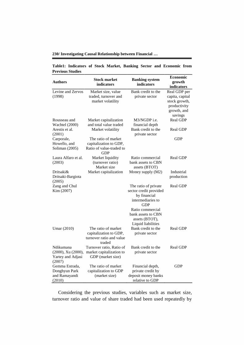
Table1: Indicators of Stock Market, Banking Sector and Economic from

Previous Studies

Authors Stock market

indicators

Banking system

indicators

Economic

growth

indicators

Levine and Zervos

(1998)

Market size, value

traded, turnover and

market volatility

Bank credit to the

private sector

Real GDP per

capita, capital

stock growth,

productivity

growth, and

savings

Rousseau and

Wachtel (2000)

Market capitalization

and total value traded

M3/NGDP i.e.

financial depth

Real GDP

Arestis et al.

(2001)

Market volatility Bank credit to the

private sector

Real GDP

Carporale,

Howello, and

Soliman (2005)

The ratio of market

capitalization to GDP,

Ratio of value-traded to

GDP

GDP

Laura Alfaro et al.

(2003)

Market liquidity

(turnover ratio)

Market size

Ratio commercial

bank assets to CBN

assets (BTOT)

Real GDP

Dritsaki&

Dritsaki-Bargiota

(2005)

Market capitalization Money supply (M2) Industrial

production

Zang and Chul

Kim (2007)

The ratio of private

sector credit provided

by financial

intermediaries to

GDP

Ratio commercial

bank assets to CBN

assets (BTOT),

Liquid liabilities

Real GDP

Umar (2010) The ratio of market

capitalization to GDP,

turnover ratio and value

traded

Bank credit to the

private sector

Real GDP

Ndikumana

(2000), Xu (2000),

Yartey and Adjasi

(2007)

Turnover ratio, Ratio of

market capitalization to

GDP (market size)

Bank credit to the

private sector

Real GDP

Gemma Estrada,

Donghyun Park

and Ramayandi

(2010)

The ratio of market

capitalization to GDP

(market size)

Financial depth,

private credit by

deposit money banks

relative to GDP

GDP

Considering the previous studies, variables such as market size,

turnover ratio and value of share traded had been used repeatedly by


many authors as indicators of the stock market. Equally, indicators

such as Credit to the private sector by all financial intermediaries

(excluding Central banks), financial depth, the ratio of commercial

bank assets to Central bank assets and money supply were used as

banking sector variables. Also, the real GDP had been used by most

authors as an indicator of economic growth.

From the foregoing, market size (MCAP_GDP), turnover ratio

(VT_MCAP) and value of share traded (TVT_GDP) were chosen as

stock markets indicators while credit to private sector (CPS_GDP),

Financial depth (M2_GDP) and ratio commercial bank assets to

Central bank assets (CMA_CBA) were used as indicators of financial

markets. Also, real GDP was used as an indicator of economic growth.

The definition of each variable is presented in what follows.

Market Size (MCAP_GDP): The size of the stock market is

measured as market capitalization divided nominal GDP. This is

denoted in the study as MCAP_GDP. The assumption underlying the

use of this variable as an indicator of stock market development is that

the size of the stock market is positively correlated with the ability to

mobilize capital and diversify risk (Levine and Zervos, 1996).

Turnover ratio (VT_MCAP): Turnover ratio computed as the

ratio of total values of trades on the major stock market exchanges

divided by market capitalization is a measure of liquidity of the stock

market. It captures the activeness or the liquidity of the stock market

size relative to its size since markets may be large but inactive. Beck

and Levine (2004) prefer this measurement to another measurement of

stock market variables. This is because unlike other measures, the

numerator and denominator of turnover ratio contain prices.

Value Traded (TVT_GDP): This is the value of all shares traded

in the stock market divided by nominal GDP. It measures how active

the stock market is as a share of the economy. While not a direct

measure of trading costs or the uncertainty associated with trading on

an exchange, theoretical models of stock market liquidity and

economic growth directly motivate Value Traded (Levine, 1991;

Bencivenga et al., 1995). Value traded measures trading volume as a

share of national output and should therefore positively reflect

liquidity on an economy-wide basis. Value Traded may be importantly

different from Turnover as shown by Demirguii-Kunt and Levine


(1996). While Value Traded captures trading relative to the size of the

economy, Turnover measures trading relative to the size of the stock

market. Thus, a small, liquid market will have high Turnover but

small-Value Traded. Since financial markets are forward-looking,

Value Traded has one potential pitfall. If markets anticipate large

corporate profits, stock prices will rise today. This price rise would

increase the value of stock transactions and therefore raise Value

Traded. Problematically, the liquidity indicator would rise without a

rise in the number of transactions or a fall in transaction costs. This

price effect plagues Capitalization too. One way to gauge the

influence of the price effect is to look at Capitalization and Value

Traded together. The price effect influences both indicators, but only

Value Traded is directly related to trading. Therefore, both market

Capitalization and Value Traded indicators are included together. If

Value Traded remains significantly correlated with growth while

controlling for Capitalization, then the price effect is not dominating

the relationship between Value Traded and growth. A second way to

gauge the importance of the price effect is to examine Turnover. The

price effect does not influence Turnover because stock prices enter the

numerator and denominator of Turnover. If Turnover is positively and

robustly associated with economic growth, then this implies that the

price effect is not dominating the relationship between liquidity and

long-run economic growth (Ross Levine and Sara Zervos, 1996).

Credit to Private Sector (CPS_GDP): This is defined as the

credit issued by all financial intermediaries (excluding Central Bank)

to the private sector divided by nominal GDP. While this measure

includes intermediaries in addition to banks, banks still account for a

major share. This indicator had been widely used in the literature. The

rationale underlying this indicator is that financial systems that

allocate more credit to private firms are more engaged in researching

firms, exerting corporate control, providing risk management services,

mobilizing savings, and facilitating transactions than financial systems

that simply funnel credit to the government or state-owned enterprises.

Financial Depth (M2_GDP): Another indicator of financial

development. Gelb (1989), Ghani (1992), King and Levine (1993a, b)

and DeGregorio and Giudotti (1995) identify a significant correlation

between financial depth and long-run economic growth rates in a


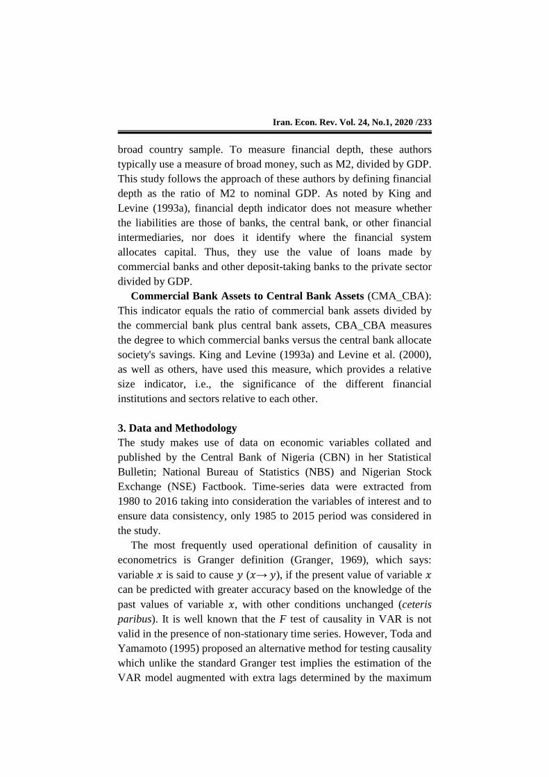
broad country sample. To measure financial depth, these authors

typically use a measure of broad money, such as M2, divided by GDP.

This study follows the approach of these authors by defining financial

depth as the ratio of M2 to nominal GDP. As noted by King and

Levine (1993a), financial depth indicator does not measure whether

the liabilities are those of banks, the central bank, or other financial

intermediaries, nor does it identify where the financial system

allocates capital. Thus, they use the value of loans made by

commercial banks and other deposit-taking banks to the private sector

divided by GDP.

Commercial Bank Assets to Central Bank Assets (CMA_CBA):

This indicator equals the ratio of commercial bank assets divided by

the commercial bank plus central bank assets, CBA_CBA measures

the degree to which commercial banks versus the central bank allocate

society's savings. King and Levine (1993a) and Levine et al. (2000),

as well as others, have used this measure, which provides a relative

size indicator, i.e., the significance of the different financial

institutions and sectors relative to each other.

3. Data and Methodology

The study makes use of data on economic variables collated and

published by the Central Bank of Nigeria (CBN) in her Statistical

Bulletin; National Bureau of Statistics (NBS) and Nigerian Stock

Exchange (NSE) Factbook. Time-series data were extracted from

1980 to 2016 taking into consideration the variables of interest and to

ensure data consistency, only 1985 to 2015 period was considered in

the study.

The most frequently used operational definition of causality in

econometrics is Granger definition (Granger, 1969), which says:

variable 𝑥 is said to cause 𝑦 (𝑥→ 𝑦), if the present value of variable 𝑥

can be predicted with greater accuracy based on the knowledge of the

past values of variable 𝑥, with other conditions unchanged (ceteris

paribus). It is well known that the F test of causality in VAR is not

valid in the presence of non-stationary time series. However, Toda and

Yamamoto (1995) proposed an alternative method for testing causality

which unlike the standard Granger test implies the estimation of the

VAR model augmented with extra lags determined by the maximum


order of integration of the series under consideration. This method is

applicable regardless of the order of integration or cointegration rank

of the observed variables.

The Toda-Yamamoto procedure of Granger non-causality test

involves four steps. Firstly, we need to find the highest order of

integration in the variables (𝑑𝑚𝑎𝑥). Determination of 𝑑𝑚𝑎𝑥 entails

conducting unit root tests on the variables and establish the level of

stationarity of the series. Dickey and Fuller (1979; 1981) suggest the

use of one of the commonly applied tests known as augmented

Dickey-Fuller (ADF) to detect whether the time series is of stationary

form.

However, the Dickey-Fuller type test may have low estimation

power against the plausible stationary alternative hypothesis and the

null hypothesis of a unit root may tend to be accepted unless there is

strong evidence against it. The Phillips-Perron (P-P) test is a non-

parametric approach to unit root test and offers an alternative method

for correcting for serial correlation in unit root testing. Basically, the

P-P test uses the standard DF or ADF test but modifies the t-ratio of

the coefficient so that serial correlation does not affect the

asymptotic distribution of the test statistic. Both ADF and P-P tests

will be used in this study and where there is a conflicting result on the

level of integration of a variable under study, P-P decision will be

upheld because of its robustness and higher power compare with

ADF.

In order to test whether the series 𝑌𝑡 contains unit root test using

the ADF test, the following equation is used

∆𝑌𝑡 = 𝛼0 + 𝛼1𝑡 + 𝛿𝑌𝑡−𝑖 + ∑ 𝜑∆𝑌𝑡−𝑖𝑁𝑖=1 + 휀𝑡 (1)

Where ∆ represent the first difference processor, 𝑡 represents a time

series trend, 휀𝑡 represents the error term. 𝑌𝑡 represents the used series,

𝑁 represents delay number determined with Akaike Information

Criterion. The ADF test considers a null hypothesis of unit root

against an alternative hypothesis that assumes the series is stable or

stationary. The test is based on the estimation of 𝛿 parameter and

determination of its test statistics. If the test statistics are greater than


the critical values in absolute value, the null hypothesis is rejected. In

other words, it can be said that the series is stable. The P-P test is

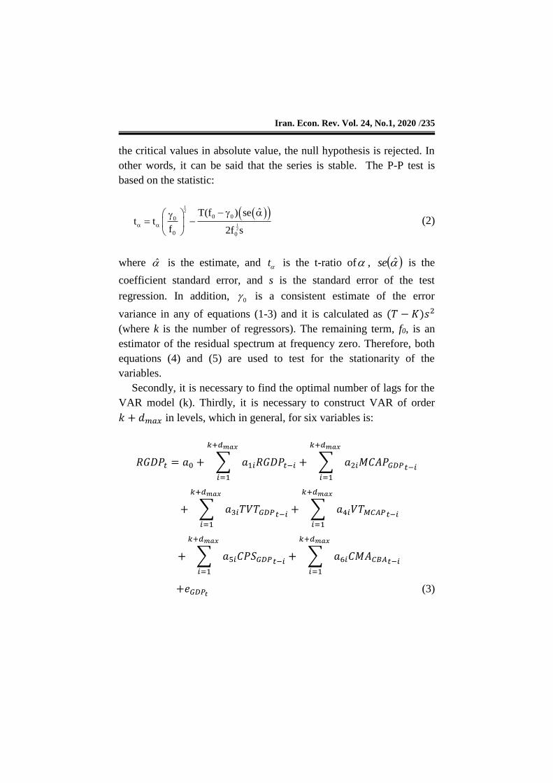
based on the statistic:

12

12

0 00

0 0

ˆT(f ) set t

f 2f s

(2)

where ̂ is the estimate, and t is the t-ratio of , ̂se is the

coefficient standard error, and s is the standard error of the test

regression. In addition, 0 is a consistent estimate of the error

variance in any of equations (1-3) and it is calculated as (𝑇 − 𝐾)𝑠2

(where k is the number of regressors). The remaining term, f0, is an

estimator of the residual spectrum at frequency zero. Therefore, both

equations (4) and (5) are used to test for the stationarity of the

variables.

Secondly, it is necessary to find the optimal number of lags for the

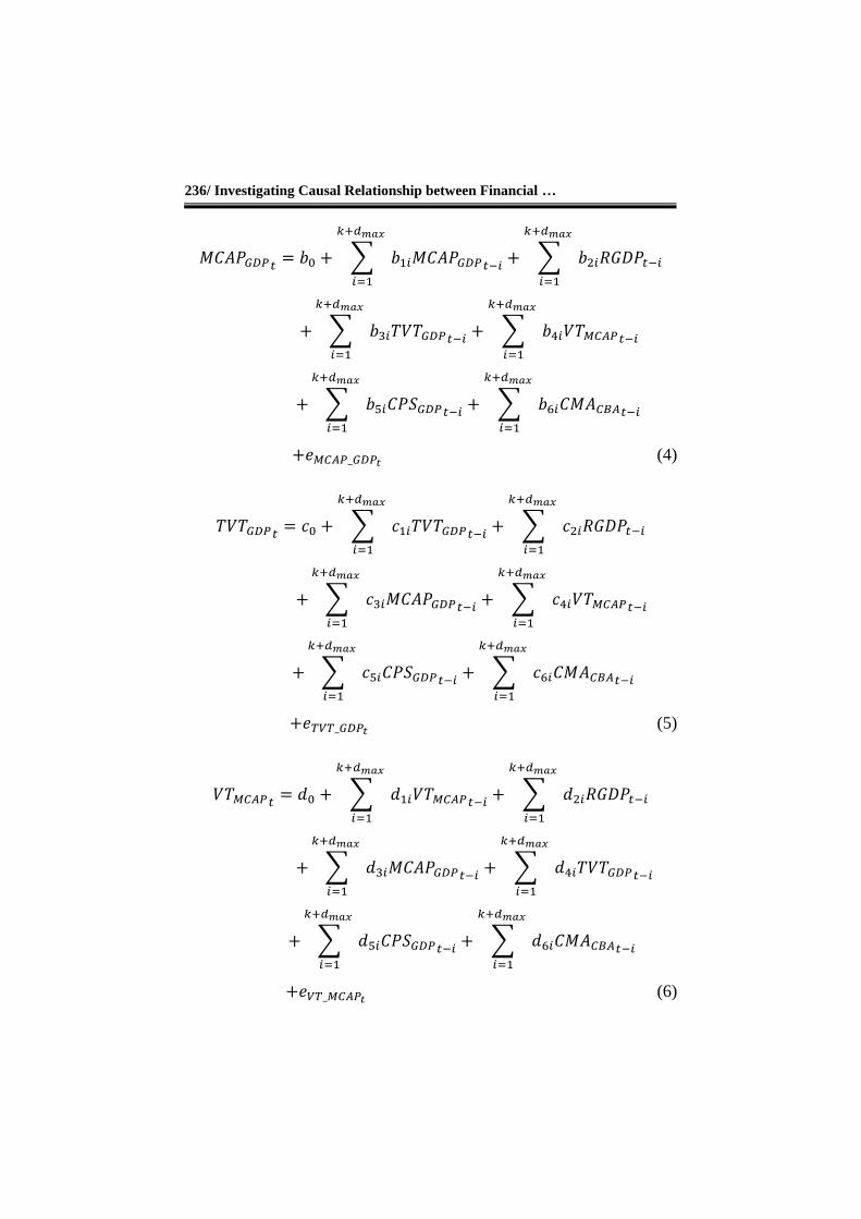
VAR model (k). Thirdly, it is necessary to construct VAR of order

𝑘 + 𝑑𝑚𝑎𝑥 in levels, which in general, for six variables is:

𝑅𝐺𝐷𝑃𝑡 = 𝑎0 + ∑ 𝑎1𝑖𝑅𝐺𝐷𝑃𝑡−𝑖

𝑘+𝑑𝑚𝑎𝑥

𝑖=1

+ ∑ 𝑎2𝑖𝑀𝐶𝐴𝑃𝐺𝐷𝑃𝑡−𝑖


𝑖=1

+ ∑ 𝑎3𝑖𝑇𝑉𝑇𝐺𝐷𝑃𝑡−𝑖


𝑖=1

+ ∑ 𝑎4𝑖𝑉𝑇𝑀𝐶𝐴𝑃𝑡−𝑖


𝑖=1

+ ∑ 𝑎5𝑖𝐶𝑃𝑆𝐺𝐷𝑃𝑡−𝑖+ ∑ 𝑎6𝑖𝐶𝑀𝐴𝐶𝐵𝐴𝑡−𝑖


𝑖=1


𝑖=1

+𝑒𝐺𝐷𝑃𝑡 (3)


𝑀𝐶𝐴𝑃𝐺𝐷𝑃𝑡= 𝑏0 + ∑ 𝑏1𝑖𝑀𝐶𝐴𝑃𝐺𝐷𝑃𝑡−𝑖


𝑖=1

+ ∑ 𝑏2𝑖𝑅𝐺𝐷𝑃𝑡−𝑖


𝑖=1

+ ∑ 𝑏3𝑖𝑇𝑉𝑇𝐺𝐷𝑃𝑡−𝑖


𝑖=1

+ ∑ 𝑏4𝑖𝑉𝑇𝑀𝐶𝐴𝑃𝑡−𝑖


𝑖=1

+ ∑ 𝑏5𝑖𝐶𝑃𝑆𝐺𝐷𝑃𝑡−𝑖+ ∑ 𝑏6𝑖𝐶𝑀𝐴𝐶𝐵𝐴𝑡−𝑖


𝑖=1


𝑖=1

+𝑒𝑀𝐶𝐴𝑃_𝐺𝐷𝑃𝑡 (4)

𝑇𝑉𝑇𝐺𝐷𝑃𝑡= 𝑐0 + ∑ 𝑐1𝑖𝑇𝑉𝑇𝐺𝐷𝑃𝑡−𝑖


𝑖=1

+ ∑ 𝑐2𝑖𝑅𝐺𝐷𝑃𝑡−𝑖


𝑖=1

+ ∑ 𝑐3𝑖𝑀𝐶𝐴𝑃𝐺𝐷𝑃𝑡−𝑖


𝑖=1

+ ∑ 𝑐4𝑖𝑉𝑇𝑀𝐶𝐴𝑃𝑡−𝑖


𝑖=1

+ ∑ 𝑐5𝑖𝐶𝑃𝑆𝐺𝐷𝑃𝑡−𝑖+ ∑ 𝑐6𝑖𝐶𝑀𝐴𝐶𝐵𝐴𝑡−𝑖


𝑖=1


𝑖=1

+𝑒𝑇𝑉𝑇_𝐺𝐷𝑃𝑡 (5)

𝑉𝑇𝑀𝐶𝐴𝑃𝑡= 𝑑0 + ∑ 𝑑1𝑖𝑉𝑇𝑀𝐶𝐴𝑃𝑡−𝑖


𝑖=1

+ ∑ 𝑑2𝑖𝑅𝐺𝐷𝑃𝑡−𝑖


𝑖=1

+ ∑ 𝑑3𝑖𝑀𝐶𝐴𝑃𝐺𝐷𝑃𝑡−𝑖


𝑖=1

+ ∑ 𝑑4𝑖𝑇𝑉𝑇𝐺𝐷𝑃𝑡−𝑖


𝑖=1

+ ∑ 𝑑5𝑖𝐶𝑃𝑆𝐺𝐷𝑃𝑡−𝑖+ ∑ 𝑑6𝑖𝐶𝑀𝐴𝐶𝐵𝐴𝑡−𝑖


𝑖=1


𝑖=1

+𝑒𝑉𝑇_𝑀𝐶𝐴𝑃𝑡 (6)


𝐶𝑃𝑆𝐺𝐷𝑃𝑡= 𝑓0 + ∑ 𝑓1𝑖𝐶𝑃𝑆𝐺𝐷𝑃𝑡−𝑖


𝑖=1

+ ∑ 𝑓2𝑖𝑅𝐺𝐷𝑃𝑡−𝑖


𝑖=1

+ ∑ 𝑓3𝑖𝑀𝐶𝐴𝑃𝐺𝐷𝑃𝑡−𝑖


𝑖=1

+ ∑ 𝑓4𝑖𝑇𝑉𝑇𝐺𝐷𝑃𝑡−𝑖


𝑖=1

+ ∑ 𝑓5𝑖𝑉𝑇𝑀𝐶𝐴𝑃𝑡−𝑖


𝑖=1

+ ∑ 𝑓6𝑖𝐶𝑀𝐴𝐶𝐵𝐴𝑡−𝑖


𝑖=1

+𝑒𝐶𝑃𝑆_𝐺𝐷𝑃𝑡 (7)

𝐶𝑀𝐴𝐶𝐵𝐴𝑡= 𝑔0 + ∑ 𝑔1𝑖𝐶𝑀𝐴𝐶𝐵𝐴𝑡−𝑖


𝑖=1

+ ∑ 𝑔2𝑖𝑅𝐺𝐷𝑃𝑡−𝑖


𝑖=1

+ ∑ 𝑔3𝑖𝑀𝐶𝐴𝑃𝐺𝐷𝑃𝑡−𝑖


𝑖=1

+ ∑ 𝑔4𝑖𝑇𝑉𝑇𝐺𝐷𝑃𝑡−𝑖


𝑖=1

+ ∑ 𝑔5𝑖𝑉𝑇𝑀𝐶𝐴𝑃𝑡−𝑖


𝑖=1

+ ∑ 𝑔6𝑖𝐶𝑃𝑆𝐺𝐷𝑃𝑡−𝑖


𝑖=1

+𝑒𝐶𝑀𝐴_𝐶𝐵𝐴𝑡 (8)

Where 𝑎0, 𝑏0, 𝑐0, 𝑑0, 𝑓0 𝑎𝑛𝑑 𝑔0 are constants, RGDP, MCAP_GDP,

TVT_GDP, VT_GDP, CPS_GDP, and CMA_CBA are the variables,

a, b, c, d, f, and g are the parameters of the model, k is the optimal lag

order, 𝑑𝑚𝑎𝑥 is the maximal order of integration of the series in the

system, 𝑒𝐺𝐷𝑃𝑡, 𝑒𝑀𝐶𝐴𝑃_𝐺𝐷𝑃𝑡

, 𝑒𝑇𝑉𝑇_𝐺𝐷𝑃𝑡, 𝑒𝑉𝑇_𝑀𝐶𝐴𝑃𝑡

, 𝑒𝑉𝑇_𝑀𝐶𝐴𝑃𝑡, 𝑒𝐶𝑃𝑆_𝐺𝐷𝑃𝑡

and 𝑒𝐶𝑀𝐴_𝐶𝐵𝐴𝑡. We estimate VAR of order (𝑘 + 𝑑𝑚𝑎𝑥) using

Seemingly Unrelated Regression (SUR) because the power of the

Wald test improves when the SUR technique is used for the estimation

(Rambaldi and Doran, 1996).

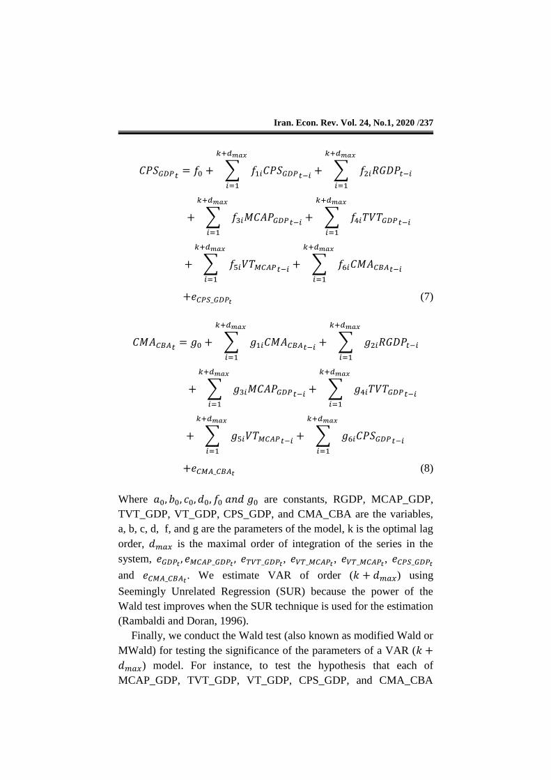
Finally, we conduct the Wald test (also known as modified Wald or

MWald) for testing the significance of the parameters of a VAR (𝑘 +

𝑑𝑚𝑎𝑥) model. For instance, to test the hypothesis that each of

MCAP_GDP, TVT_GDP, VT_GDP, CPS_GDP, and CMA_CBA


does not Granger cause RGDP from equation (3), we test

H0: a2i, a3i, a4i, a5i = 0 against 𝐻1: 𝑎2𝑖 , 𝑎3𝑖, 𝑎4𝑖, 𝑎5𝑖 ≠ 0. (𝑖 = 1 … 𝑘).

In the same vein, to test the hypothesis “RGDP, TVT_GDP,

VT_GDP, CPS_GDP, and CMA_CBA does not Granger cause

MCAP_GDP” from equation (4), we test, H0: b2i, b3i, b4i, b5i = 0

against 𝐻1: 𝑏2𝑖 , 𝑏3𝑖, 𝑏4𝑖, 𝑏5𝑖 ≠ 0. Similarly, the procedure is repeated

until all the variables in the VAR system are covered. Wald test is

then applied on the first k coefficient matrices, whereas the coefficient

matrices of the last 𝑑𝑚𝑎𝑥 lagged vectors in the model are ignored

(since they are regarded as zeros). In that case, the Wald test statistics

follow asymptotic 𝜒2 distribution with m degrees of freedom and it

can be applied even if the X variables in the system are I(0), I(1) or

I(2), cointegrated or non-cointegrated with a condition that the order

of integration does not exceed the true lag length of the model (Toda

and Yamamoto, 1995).

4. Data Analysis and Result Discussion

Every other variable in this study is in ratio form apart from real GDP

and this necessitates its logarithm transformation prior to the analysis.

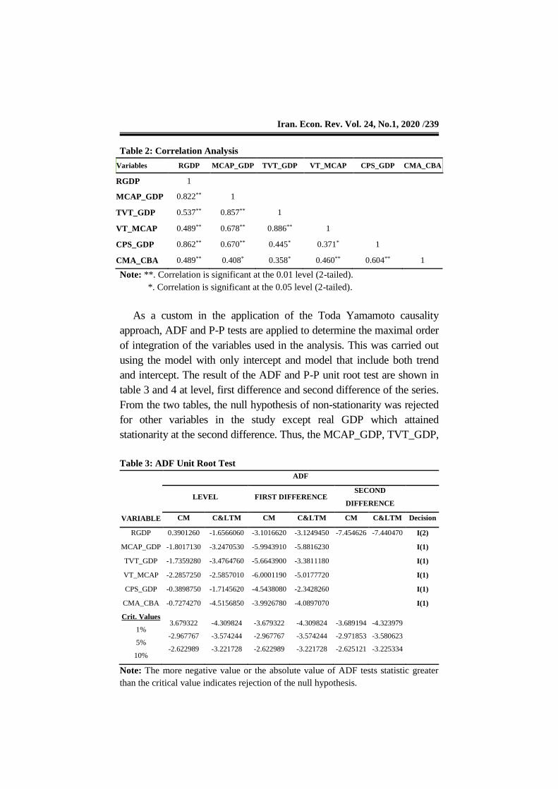
At the onset, Pearson Product Moment Correlation analysis was

carried out among the variables over the sample period and its

significance was established using a t-test. The correlation matrix

presented in Table 2 showed a positive and significant correlation

among the variables. That is each pair of the variable tend to move in

the same direction. Also, there is a very high degree of correlation

between market size (MCAP_GDP), Credit to the private sector

(CPS_GDP) and Real GDP while other variables moderately

correlated with Real GDP. In addition, (M2_GDP) was removed from

the analysis due to its near-perfect association with another variable in

the system. Correlation, however, does not say anything about a

causal relationship and thus, leaves unsettled the debate concerning

the causal relationship between financial market and economic growth

of the country under consideration.


Table 2: Correlation Analysis

Variables RGDP MCAP_GDP TVT_GDP VT_MCAP CPS_GDP CMA_CBA

RGDP 1

MCAP_GDP 0.822** 1

TVT_GDP 0.537** 0.857** 1

VT_MCAP 0.489** 0.678** 0.886** 1

CPS_GDP 0.862** 0.670** 0.445* 0.371* 1

CMA_CBA 0.489** 0.408* 0.358* 0.460** 0.604** 1

Note: **. Correlation is significant at the 0.01 level (2-tailed).

*. Correlation is significant at the 0.05 level (2-tailed).

As a custom in the application of the Toda Yamamoto causality

approach, ADF and P-P tests are applied to determine the maximal order

of integration of the variables used in the analysis. This was carried out

using the model with only intercept and model that include both trend

and intercept. The result of the ADF and P-P unit root test are shown in

table 3 and 4 at level, first difference and second difference of the series.

From the two tables, the null hypothesis of non-stationarity was rejected

for other variables in the study except real GDP which attained

stationarity at the second difference. Thus, the MCAP_GDP, TVT_GDP,

Table 3: ADF Unit Root Test

VARIABLE

ADF

LEVEL FIRST DIFFERENCE SECOND

DIFFERENCE

CM C&LTM CM C&LTM CM C&LTM Decision

RGDP 0.3901260 -1.6566060 -3.1016620 -3.1249450 -7.454626 -7.440470 I(2)

MCAP_GDP -1.8017130 -3.2470530 -5.9943910 -5.8816230 I(1)

TVT_GDP -1.7359280 -3.4764760 -5.6643900 -3.3811180 I(1)

VT_MCAP -2.2857250 -2.5857010 -6.0001190 -5.0177720 I(1)

CPS_GDP -0.3898750 -1.7145620 -4.5438080 -2.3428260 I(1)

CMA_CBA -0.7274270 -4.5156850 -3.9926780 -4.0897070 I(1)

Crit. Values

1%

5%

10%

3.679322

-2.967767

-2.622989

-4.309824

-3.574244

-3.221728

-3.679322

-2.967767

-2.622989

-4.309824

-3.574244

-3.221728

-3.689194

-2.971853

-2.625121

-4.323979

-3.580623

-3.225334

Note: The more negative value or the absolute value of ADF tests statistic greater

than the critical value indicates rejection of the null hypothesis.


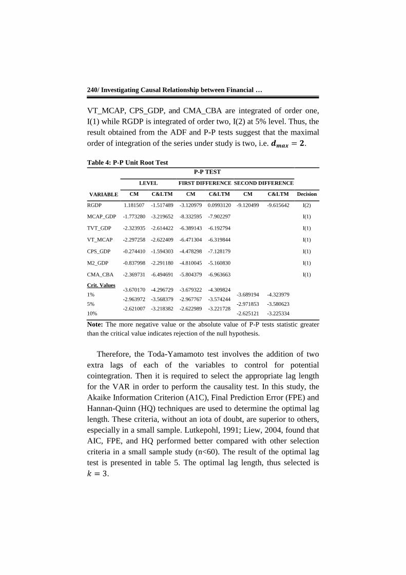
VT_MCAP, CPS_GDP, and CMA_CBA are integrated of order one,

I(1) while RGDP is integrated of order two, I(2) at 5% level. Thus, the

result obtained from the ADF and P-P tests suggest that the maximal

order of integration of the series under study is two, i.e. 𝒅𝒎𝒂𝒙 = 𝟐.

Table 4: P-P Unit Root Test

VARIABLE

P-P TEST

LEVEL FIRST DIFFERENCE SECOND DIFFERENCE

CM C&LTM CM C&LTM CM C&LTM Decision

RGDP 1.181507 -1.517489 -3.120979 0.0993120 -9.120499 -9.615642 I(2)

MCAP_GDP -1.773280 -3.219652 -8.332595 -7.902297 I(1)

TVT_GDP -2.323935 -2.614422 -6.389143 -6.192794 I(1)

VT_MCAP -2.297258 -2.622409 -6.471304 -6.319844 I(1)

CPS_GDP -0.274410 -1.594303 -4.478298 -7.128179 I(1)

M2_GDP -0.837998 -2.291180 -4.810045 -5.160830 I(1)

CMA_CBA -2.369731 -6.494691 -5.804379 -6.963663 I(1)

Crit. Values

1%

5%

10%

-3.670170

-2.963972

-2.621007

-4.296729

-3.568379

-3.218382

-3.679322

-2.967767

-2.622989

-4.309824

-3.574244

-3.221728

-3.689194

-2.971853

-2.625121

-4.323979

-3.580623

-3.225334

Note: The more negative value or the absolute value of P-P tests statistic greater

than the critical value indicates rejection of the null hypothesis.

Therefore, the Toda-Yamamoto test involves the addition of two

extra lags of each of the variables to control for potential

cointegration. Then it is required to select the appropriate lag length

for the VAR in order to perform the causality test. In this study, the

Akaike Information Criterion (A1C), Final Prediction Error (FPE) and

Hannan-Quinn (HQ) techniques are used to determine the optimal lag

length. These criteria, without an iota of doubt, are superior to others,

especially in a small sample. Lutkepohl, 1991; Liew, 2004, found that

AIC, FPE, and HQ performed better compared with other selection

criteria in a small sample study (n<60). The result of the optimal lag

test is presented in table 5. The optimal lag length, thus selected is

𝑘 = 3.


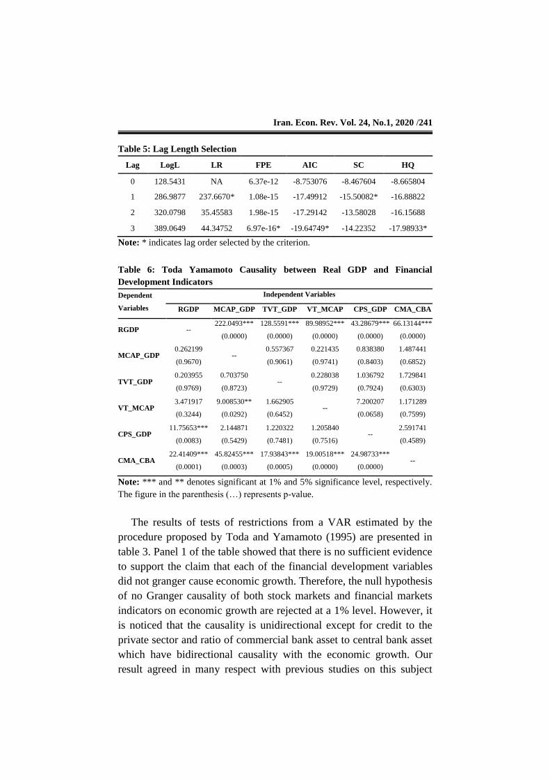
Table 5: Lag Length Selection

Lag LogL LR FPE AIC SC HQ

0 128.5431 NA 6.37e-12 -8.753076 -8.467604 -8.665804

1 286.9877 237.6670* 1.08e-15 -17.49912 -15.50082* -16.88822

2 320.0798 35.45583 1.98e-15 -17.29142 -13.58028 -16.15688

3 389.0649 44.34752 6.97e-16* -19.64749* -14.22352 -17.98933*

Note: * indicates lag order selected by the criterion.

Table 6: Toda Yamamoto Causality between Real GDP and Financial

Development Indicators

Dependent

Variables

Independent Variables

RGDP MCAP_GDP TVT_GDP VT_MCAP CPS_GDP CMA_CBA

RGDP -- 222.0493***

(0.0000)

128.5591***

(0.0000)

89.98952***

(0.0000)

43.28679***

(0.0000)

66.13144***

(0.0000)

MCAP_GDP 0.262199

(0.9670) --

0.557367

(0.9061)

0.221435

(0.9741)

0.838380

(0.8403)

1.487441

(0.6852)

TVT_GDP 0.203955

(0.9769)

0.703750

(0.8723) --

0.228038

(0.9729)

1.036792

(0.7924)

1.729841

(0.6303)

VT_MCAP 3.471917

(0.3244)

9.008530**

(0.0292)

1.662905

(0.6452) --

7.200207

(0.0658)

1.171289

(0.7599)

CPS_GDP 11.75653***

(0.0083)

2.144871

(0.5429)

1.220322

(0.7481)

1.205840

(0.7516) --

2.591741

(0.4589)

CMA_CBA 22.41409***

(0.0001)

45.82455***

(0.0003)

17.93843***

(0.0005)

19.00518***

(0.0000)

24.98733***

(0.0000) --

Note: *** and ** denotes significant at 1% and 5% significance level, respectively.

The figure in the parenthesis (…) represents p-value.

The results of tests of restrictions from a VAR estimated by the

procedure proposed by Toda and Yamamoto (1995) are presented in

table 3. Panel 1 of the table showed that there is no sufficient evidence

to support the claim that each of the financial development variables

did not granger cause economic growth. Therefore, the null hypothesis

of no Granger causality of both stock markets and financial markets

indicators on economic growth are rejected at a 1% level. However, it

is noticed that the causality is unidirectional except for credit to the

private sector and ratio of commercial bank asset to central bank asset

which have bidirectional causality with the economic growth. Our

result agreed in many respect with previous studies on this subject


matter. One example of these studies is Dritsaki & Dritsaki-Bargiota

(2005) using a tri-variate VAR model to examine the causal

relationship between credit stock, credit market and economic growth

for Greece. Like this study, their results reveal unidirectional causality

from economic development to stock market indicators and

bidirectional causality between economic developments and banking

sector variables also establishes no causal relationship between stock

market function and banking sector.

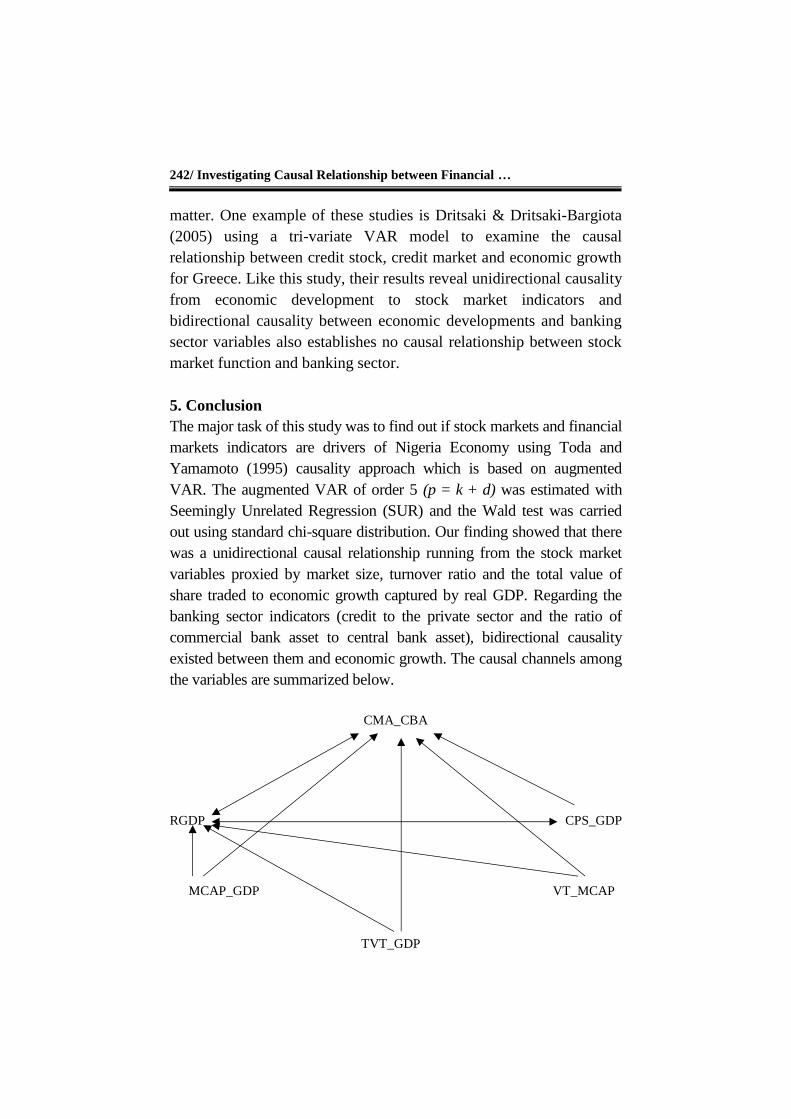
5. Conclusion

The major task of this study was to find out if stock markets and financial

markets indicators are drivers of Nigeria Economy using Toda and

Yamamoto (1995) causality approach which is based on augmented

VAR. The augmented VAR of order 5 (p = k + d) was estimated with

Seemingly Unrelated Regression (SUR) and the Wald test was carried

out using standard chi-square distribution. Our finding showed that there

was a unidirectional causal relationship running from the stock market

variables proxied by market size, turnover ratio and the total value of

share traded to economic growth captured by real GDP. Regarding the

banking sector indicators (credit to the private sector and the ratio of

commercial bank asset to central bank asset), bidirectional causality

existed between them and economic growth. The causal channels among

the variables are summarized below.

CMA_CBA

RGDP CPS_GDP

MCAP_GDP VT_MCAP

TVT_GDP


The deduction from the result reiterated the fact that the financial

sector plays a crucial role in the Nigeria economy. The unidirectional

causality from the stock market indicators to economic growth

suggests that the development of stock markets contributes to

economic growth rather than stating that stock markets develop as the

economy develops. It also indicates that growth is not a good indicator

for predicting stock returns. Furthermore, the already established fact

from the study that credit market expansion as measured by bank

credit to private sector leads to economic growth can be explained in

the sense that, with the expansion of bank credit to private sector,

more innovative projects are to be undertaken and as a result,

investment, employment, and output will increase putting the

country's economy on a path of growth. However, the most recent

global financial crisis is there to remind us that the banking sector is

arguably the most cyclical and risk-prone sectors of the economy and

the private sector is the most unaccountable sector.

In a developing economy like Nigeria, oil dependency is a major

determinant on how stocks and financial Institutions stimulate

economic growth, sadly there is little control over how oil shocks can

be minimized especially on an international scale.

Government policies aimed at reducing dependency on crude oil

and gas export as a major source of revenue and improvement of

foreign investments may help in projecting how much financial

development activates economic growth, sustainably. There is a need

to continue with these reforms to enable it to contribute effectively to

economic growth. However, a lot still needs to be done in translating

this achievement to the proper growth process.

Based on this result, it will not be misleading to assert that reforms

and restructuring that can boost financial markets and diminish

dependence on natural resources should be pursued by the developing

countries. This will provide panacea and rescue for the economy in

case of an unforeseen crisis in the oil sector. Diversification of

Economy and a strengthened financial sector is unavoidable for

survival in times of global crisis.


References

Arestis, P., Demetriades, P. O., & Luintel, K. B. (2001). Financial

Development and Economic Growth: The Role of the Stock Market.

Journal of Money, Credit and Banking, 33(1), 16-41.

Bencivenga, V. R., Smith, B. D., & Starr, R. M. (1995). Transactions

Costs, Technological Choice, and Endogenous Growth. Journal of

Economic Theory, 67(1), 53-177.

Black, J. (2002). Oxford Dictionary of Economics (2nd Ed.). Oxford:

Oxford University Press.

De Gregorio, J., & Giudotti, P. E. (1995). Financial Development and

Economic Growth. World Development, 23(3), 433-448.

Dickey, D. A., & Fuller, W. A. (1979). Distribution of Estimators for

Autoregressive Time Series with a Unit Root. Journal of the American

Statistical Association, 74, 427-431.

---------- (1981). Likelihood Ratio Statistics for Autoregressive Time

Series with a Unit Root. Econometrica, 49, 1057-1072.

Dolado, J. J., & Lütkepohl, H. (1996). Making Wald Tests Work for

Cointegrated VAR System. Econometric Reviews, 15(4), 369-386.

Dritsaki, C., & Dritsaki-Bargiota, M. (2005). The Causal Relationship

between Stock, Credit Market, and Economic Development: An

Empirical Evidence for Greece. Economic Change and Restructuring,

38, 113-127.

Estrada, G. B., Park, D., & Ramayandi, A. (2010). Financial

Development and Economic Growth in Developing Asia. Asian

Development Bank Economics Working Paper, 233, Retrieved from

https://ssrn.com/abstract=1751833.

Gelb, A. H. (1989). Financial Policies, Growth and Efficiency.

Retrieved from https://books.google.com.

https://ssrn.com/abstract=1751833


Ghani, E. (1992). How Financial Markets Affect Long-Run Growth: A

Cross-Country Study. Washington, DC: World Bank.

Granger, C. W. J. (1969). Investigating Causal Relations by

Econometric Models and Cross Spectral Methods. Econometrica, 37,

424-438.

Gulmez, A., Besel, F., & Yardimcioglu, F. (2017). Does Country

Credit Rating Affect Current Deficit Account? Journal of Economic

and Social Research, 3(2), 25-42.

King, R. G., & Levine, R. (1993). Finance and Growth: Schumpeter

Might Be Right. Quarterly Journal of Economics, 108(3), 717-738.

Lall, S. V., Henderson, V. M., & Venables, A. J. (2017). Africa's

Cities Opening Doors to the World. Washington, DC: World Bank

Group.

Levine, R. (1997). Financial Development and Economic growth:

Views and Agenda. Journal of Economic Literature, 35(2), 688-726.

---------- (1991). Stock Markets, Growth, and Tax Policy. Journal of

Finance, 46(4), 1445-1165.

Levine, R., & Zervos, S. (1998). Stock Markets, Banks, and Economic

Growth. American Economic Review, 88(3), 537-558.

Levine, R., Loayza, N., & Beck, T. (2000). Financial Intermediation

and Growth: Causality and Causes. Journal of Monetary Economics,

46(1), 31-77.

Liew, K. S. (2004). Which Lag Length Selection Criteria should we

employ? Economics Bulletin, 3(33), 1-9.

Lucas, R. E. (1988). On the Mechanics of Economic Development.

Journal of Monetary Economics, 22, 3-42.


Lutkepohl, H. (1991). Introduction to Multiple Time Series Analysis.

Germany: Springer.

Ndikumana, L. (2000). Financial Determinants of Domestic

Investment in Sub-Sahara Africa: Evidence from Panel Data. World

Development, 28(2), 381-400.

Rioja, F., & Valen, N. (2014). Stock Markets, Banks and the Sources

of Economic Growth in Low and High-Income Countries. Retrieved

from www2.gsu.edu/~ecofkr/papers/JEF_rioja_valev_2012.pdf .

Rousseau, P. L., & Wachtel, P. (2000). Equity Market and Growth:

Cross-country Evidence on Timing and Outcomes, 1980-1995.

Journal of Banking and Finance, 24, 1933-1957.

Toda, H. Y., & Yamamoto, T. (1995). Statistical Inference in Vector

Autoregressions with Possibly Integrated Process. Journal of

Econometrics, 66(1-2), 225-250.

Umar, B. N. (2010). Stock Markets, Banks and Economic Growth:

Time Series Evidence from South Africa. The African Finance

Journal, 12(2), 72-92.

Xu, Z. (2000). Financial Development, Investment, and Economic

Growth. Economic Inquiry, 38(2), 331-344.

Zang, H., & Chul Kim, Y. (2007). Does Financial Development

Precede Growth? Robinson and Lucas Might be Right. Applied

Economic Letters, 14, 15-19.

https://www.google.com.ng/url?sa=t&rct=j&q=&esrc=s&source=web&cd=1&cad=rja&uact=8&ved=2ahUKEwiC6Nms_sneAhVS1lMKHUaXBCgQFjAAegQIARAC&url=http%3A%2F%2Fwww2.gsu.edu%2F~ecofkr%2Fpapers%2FJEF_rioja_valev_2012.pdf&usg=AOvVaw3vDtSGZFqlR6anikMSC_sX

https://ideas.repec.org/a/afj/journl/v12y2010i2p72-92.html

https://ideas.repec.org/a/afj/journl/v12y2010i2p72-92.html

https://ideas.repec.org/s/afj/journl.html

https://ideas.repec.org/s/afj/journl.html

Documents

Investigating Causal Relationship between Financial ... · between financial development and economic growth in Nigeria for the period 1985 to 2015. TYDL is based on an augmented