Ionospheric perturbations linked to a very powerful seismic event

ARTICLE IN PRESS

1364-6826/$ - se

doi:10.1016/j.ja

�Correspondfax: +33238 63

E-mail addr

(Y. Hobara).1Present addr

SE-981 28 Kiru

Journal of Atmospheric and Solar-Terrestrial Physics 67 (2005) 677–685

www.elsevier.com/locate/jastp

Ionospheric perturbations linked to a very powerfulseismic event

Y. Hobara�,1, M. Parrot

LPCE/CNRS, 3A Avenue de la Recherche Scientifique, 45071 Orleans Cedex 2, France

Received 13 January 2003; received in revised form 27 January 2004; accepted 2 February 2005

Abstract

Ionospheric anomalies in association with the powerful Hachinohe earthquake (M ¼ 8:3) are derived using foF2 (F2

layer O-mode critical frequency) records from worldwide ionospheric stations. The results show that meaningful

decreases in foF2 are identified only at several ionospheric stations near the epicenter, indicating that the anomalies

extend to about 1500 km from the epicenter. These anomalies are observed a couple of days before and/or after the

main shock and the duration of each anomaly is one-day. The anomalies occur predominantly during daytime.

r 2005 Elsevier Ltd. All rights reserved.

Keywords: Ionospheric perturbation; Earthquake; Ionospheric sounding; F-region

1. Introduction

Electromagnetic perturbations due to seismic activity

have been known for a long time (Milne, 1890). Due to a

lack of complete measurements, they have been the

object of large debate in the literature. Variations of

ionospheric parameters above seismically active regions

are one aspect of these perturbations. The aim of this

paper is to study the ionospheric data recorded by the

ground-based ionospheric sounders around a powerful

earthquake as a case study.

The ionosphere is mainly under the control of the

solar wind and it suffers from large geomagnetic

activity. Therefore, a perturbation coming from the

Earth’s surface or induced in the lower ionosphere is not

e front matter r 2005 Elsevier Ltd. All rights reserve

stp.2005.02.006

ing author. Tel. +33238 255291;

1234.

esses: [email protected], [email protected]

ess: Swedish Institute of Space Physics, Box 812,

na, Sweden.

easy to detect and to characterise. It is clear that during

and after an earthquake the generated acoustic-gravity

waves (GW) perturb the ionosphere due to their

intensity increasing with decreasing atmospheric density

(Blanc, 1985; Calais and Minster, 1995; Yuen et al.,

1969, and references therein). The phenomena which

could occur in some cases before earthquakes are not so

evident. Some papers have been published concerning

these events see for example, (Liu et al., 2000, 2001;

Pulinets et al., 2001; Boyarchuk et al., 2001). A recent

review concerning E sporadic layer modifications is also

given in Liperovsky et al. (2000). Many points remain

unclear concerning these pre-earthquake effects, and this

paper will attempt to answer the following questions

using a clear example from a very powerful earthquake:

Does the phenomena correspond to a decrease or an

increase of the ionospheric electron density? Is there a

special local time to observe them? What is the time

interval before their occurrence and the earthquakes

(lead time)? And what is the spatial extent of anomaly?

In this paper, we firstly describe our source of

ionospheric and seismic data (Section 2), and then

d.

www.elsevier.com/locate/jastp

ARTICLE IN PRESS

60

70

f

Y. Hobara, M. Parrot / Journal of Atmospheric and Solar-Terrestrial Physics 67 (2005) 677–685678

demonstrate the temporal dependence of characteristic

frequency in association with the Hachinohe earthquake

(Section 3) and finally discuss our results in Section 4.

10

20

30

40

50

50 100 150 200 250 300Longitude [deg]

Epicenter

ge

ca

bd

h

i

j

Lat

itude

[de

g]

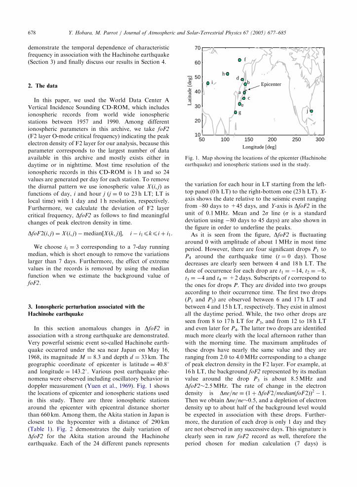
Fig. 1. Map showing the locations of the epicenter (Hachinohe

earthquake) and ionospheric stations used in the study.

2. The data

In this paper, we used the World Data Center A

Vertical Incidence Sounding CD-ROM, which includes

ionospheric records from world wide ionospheric

stations between 1957 and 1990. Among different

ionospheric parameters in this archive, we take foF2

(F2 layer O-mode critical frequency) indicating the peak

electron density of F2 layer for our analysis, because this

parameter corresponds to the largest number of data

available in this archive and mostly exists either in

daytime or in nighttime. Most time resolution of the

ionospheric records in this CD-ROM is 1 h and so 24

values are generated per day for each station. To remove

the diurnal pattern we use ionospheric value X ði; jÞ as

functions of day, i and hour j (j ¼ 0 to 23 h LT; LT is

local time) with 1 day and 1 h resolution, respectively.

Furthermore, we calculate the deviation of F2 layer

critical frequency, DfoF2 as follows to find meaningful

changes of peak electron density in time.

DfoF2ði; jÞ ¼ X ði; jÞ �median X ðk; jÞ½ �; i � i1pkpi þ i1.

We choose i1 ¼ 3 corresponding to a 7-day running

median, which is short enough to remove the variations

larger than 7 days. Furthermore, the effect of extreme

values in the records is removed by using the median

function when we estimate the background value of

foF2.

3. Ionospheric perturbation associated with the

Hachinohe earthquake

In this section anomalous changes in DfoF2 in

association with a strong earthquake are demonstrated.

Very powerful seismic event so-called Hachinohe earth-

quake occurred under the sea near Japan on May 16,

1968, its magnitude M ¼ 8:3 and depth d ¼ 33 km. The

geographic coordinate of epicenter is latitude ¼ 40.81

and longitude ¼ 143.21. Various post earthquake phe-

nomena were observed including oscillatory behavior in

doppler measurement (Yuen et al., 1969). Fig. 1 shows

the locations of epicenter and ionospheric stations used

in this study. There are three ionospheric stations

around the epicenter with epicentral distance shorter

than 660 km. Among them, the Akita station in Japan is

closest to the hypocenter with a distance of 290 km

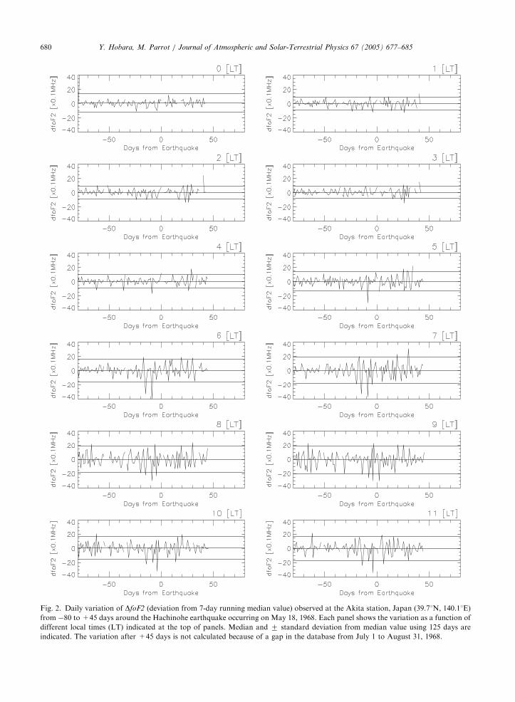
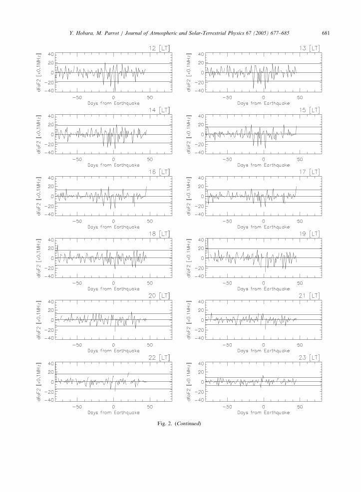
(Table 1). Fig. 2 demonstrates the daily variation of

DfoF2 for the Akita station around the Hachinohe

earthquake. Each of the 24 different panels represents

the variation for each hour in LT starting from the left-

top panel (0 h LT) to the right-bottom one (23 h LT). X-

axis shows the date relative to the seismic event ranging

from –80 days to +45 days, and Y-axis is DfoF2 in the

unit of 0.1MHz. Mean and 2s line (s is a standard

deviation using �80 days to 45 days) are also shown in

the figure in order to underline the peaks.

As it is seen from the figure, DfoF2 is fluctuating

around 0 with amplitude of about 1MHz in most time

period. However, there are four significant drops P1 to

P4 around the earthquake time (t ¼ 0 day). Those

decreases are clearly seen between 4 and 18 h LT. The

date of occurrence for each drop are t1 ¼ �14, t2 ¼ �8,

t3 ¼ �4 and t4 ¼ +2 days. Subscripts of t correspond to

the ones for drops P. They are divided into two groups

according to their occurrence time. The first two drops

(P1 and P2) are observed between 6 and 17 h LT and

between 4 and 15 h LT, respectively. They exist in almost

all the daytime period. While, the two other drops are

seen from 8 to 17 h LT for P3, and from 12 to 18 h LT

and even later for P4. The latter two drops are identified

much more clearly with the local afternoon rather than

with the morning time. The maximum amplitudes of

these drops have nearly the same value and they are

ranging from 2.0 to 4.0MHz corresponding to a change

of peak electron density in the F2 layer. For example, at

16 h LT, the background foF2 represented by its median

value around the drop P3 is about 8.5MHz and

DfoF2�2.5MHz. The rate of change in the electron

density is Dne=ne ¼ ð1þ DfoF2=medianðfoF2ÞÞ2 � 1.

Then we obtain Dne/ne�0.5, and a depletion of electron

density up to about half of the background level would

be expected in association with these drops. Further-

more, the duration of each drop is only 1 day and they

are not observed in any successive days. This signature is

clearly seen in raw foF2 record as well, therefore the

period chosen for median calculation (7 days) is

ARTICLE IN PRESS

Table 1

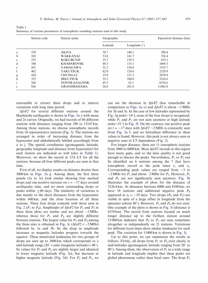
Summary of various parameters of ionospheric sounding stations used in this study

Station code Station name Geographic Epicentral distance (km)

Latitude Longitude (1)

a 539 AKITA 39.7 140.1 290.4

b 545 WAKKANAI 53.8 141.7 526.4

c 535 KOKUBUNJI 35.7 139.5 653.3

d 548 KHABAROVSK 48.5 135.1 1069.3

e 431 YAMAGAWA 31.2 130.6 1555.7

f 462 YAKUTSUK 62.0 129.6 2529.9

g 424 CHUNG-LI 25.0 121.5 2670.9

h 352 IRKUTSUK 52.5 104.0 3216.6

i 246 NOVOKAZALINSK 45.5 62.1 6318.6

j 926 GRANDBAHAMA 26.6 281.8 11402.0

Y. Hobara, M. Parrot / Journal of Atmospheric and Solar-Terrestrial Physics 67 (2005) 677–685 679

reasonable to extract these drops and to remove

variations with long time period.

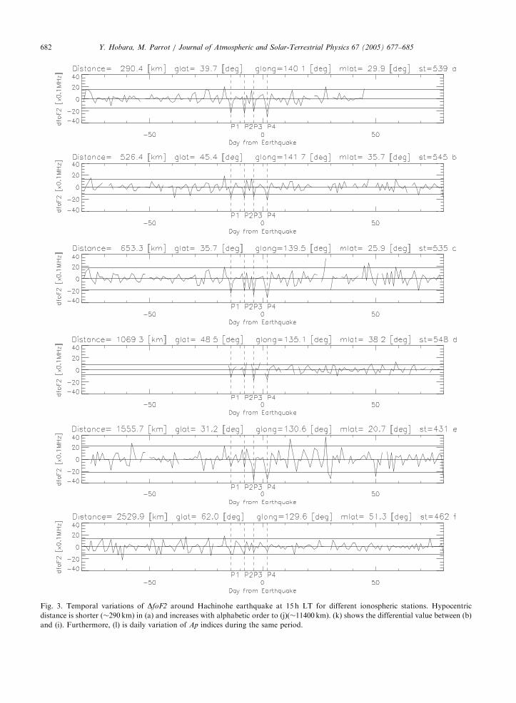
DfoF2 for several different stations around the

Hachinohe earthquake is shown in Figs. 3a–j with mean

and 2s curves. Originally, we had records of 60 different

stations with distances ranging from 290 to 13147 km.

Among those stations, we choose ionospheric records

from 10 representative stations (Fig. 3). The stations are

arranged in order of increasing distance from the

hypocenter and alphabetically labeled accordingly from

a to j. The spatial coordinates (geomagnetic latitude,

geographic longitude and distance from hypocenter) for

each station are indicated as well (also in Table 1).

Moreover, we show the record at 15 h LT for all the

stations, because all four different peaks are seen at that

time.

First of all, we display results on distance shorter than

3000 km in Figs. 3a–g. Among them, the first three

panels (3a to 3c) look similar showing four marked

drops and one positive increase on t ¼ �17 days around

earthquake time, and no more outstanding drops or

peaks within 780 days. The similarity of variations is

due mainly to the short distances from the hypocenter

within 660 km, and the close location of all three

stations. These four drops coincide with those seen in

Fig. 2 (P1 to P4). Amplitudes of DfoF2 for P1 and P2 in

these three plots are similar and are about �2MHz,

whereas those for P3 and P4 are slightly different

between stations. The largest value for P3 and P4 among

the three sites is obtained in Fig. 3c (DfoF2o�2MHz)

followed by 3a and 3b. So the drop in amplitude

increases as magnetic latitudes progress towards the

equator. These mentioned tendencies for two groups of

drops are seen up to 3000 km which corresponds to a

mid-latitude range (201omlat (magnetic latitude)o401).

So values for P3 and P4 are slightly larger and identical

in lower magnetic latitude (Fig. 3e), but decrease at

higher magnetic latitude (Fig. 3d). For P1 and P2, we

can see the decrease in DfoF2 (less remarkable in

comparison to Figs. 3a–c) and DfoF2 is about �1MHz

for 3d and 3e. In the case of low latitudes represented by

Fig. 3g (mlat�141), none of the four drops is recognized,

while P1 and P2 are not seen anymore at high latitude

(mlat�511) in Fig. 3f. On the contrary one positive peak

on t ¼ �17 days with DfoF2 �2MHz is constantly seen

from Fig. 3a–f, and no latitudinal difference in these

values is found. However, this peak is not always seen as

negative ones in LT dependence (Fig. 2).

For longer distance, there are 11 ionospheric stations

from 3000 to 6000 km. Most DfoF2 records in this region

have many gaps, and so the data quality is not good

enough to discuss the peaks. Nevertheless, P1 or P2 can

be identified on 6 stations among the 7 that have

ionospheric record at the peak times t1 and t2.

Corresponding peak values are ranged from �3 to

�2MHz for P1 and about –2MHz for P2. However, P3

and P4 are not significantly seen anymore. Fig. 3h

illustrates the example of plots for the distance of

3126.6 km. At distances between 6000 and 8100 km, we

have 18 stations and additional negative peak P0

appeared at t0 ¼ �19 days. Two drops (P0 and P1) are

visible in spite of a large offset in longitude from the

epicenter (about 801). However, P3 and P4 do not exist.

One example of the plots is shown in Fig. 3i (distance is

6319 km). The record from stations located on much

longer distance up to the farthest station around

13 000 km indicates that P0 to P2 are seen sometimes

altogether or independently on 21 stations. Variations

for different local times show similar tendencies for each

peak. The variation for 11400 km is shown in Fig. 3j.

Up to this point, we can summarize the results as

follows. Firstly, all drops from P1 to P4 exist clearly at

mid-latitudes (geomagnetic latitude ranging from 201 to

401). Among them, the observation of P1 in a wide range

in latitude and longitude implies that these peaks are

global phenomena rather than local ones. The drop P2

ARTICLE IN PRESS

Fig. 2. Daily variation of DfoF2 (deviation from 7-day running median value) observed at the Akita station, Japan (39.71N, 140.11E)

from �80 to +45 days around the Hachinohe earthquake occurring on May 18, 1968. Each panel shows the variation as a function of

different local times (LT) indicated at the top of panels. Median and 7 standard deviation from median value using 125 days are

indicated. The variation after +45 days is not calculated because of a gap in the database from July 1 to August 31, 1968.


ARTICLE IN PRESS

Fig. 2. (Continued)


ARTICLE IN PRESS

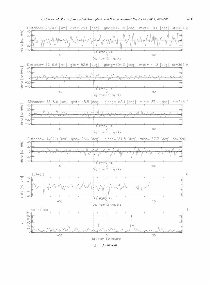
Fig. 3. Temporal variations of DfoF2 around Hachinohe earthquake at 15 h LT for different ionospheric stations. Hypocentric

distance is shorter (�290 km) in (a) and increases with alphabetic order to (j)(�11400 km). (k) shows the differential value between (b)

and (i). Furthermore, (l) is daily variation of Ap indices during the same period.


ARTICLE IN PRESS

Fig. 3. (Continued)


ARTICLE IN PRESSY. Hobara, M. Parrot / Journal of Atmospheric and Solar-Terrestrial Physics 67 (2005) 677–685684

might be due to the solar activity (geomagnetic storm

effect) because of increasing Ap index one day before the

drop P2 (Fig. 3(l)). On the contrary, P3 and P4 are only

seen up to 1500 km from the hypocenter, and are

particularly limited either in latitude or longitude ranges

near the epicenter (201omlat o501 and 1311 Eolong

(geographic longitude) o1421 E) indicating the special

extent of the disturbed region. Moreover, Ap indices in

these days are not large (quiet enough) except at date of

P2 and do not seem to disturb significantly the

ionosphere (Fig. 3(l)). So P3 and P4 can be associated

with this powerful seismic event. In this event, the sign

of DfoF2 is negative and the leading time of the drop P3

is 4 days before the earthquake, and the other drop P4 is

2 days after the shock. Both drops are only seen in one

day, associated amplitude change is about 3MHz with a

maximum at 15 h LT, and the observed period is

predominantly in the afternoon.

For further confirmation of the spatial difference

between the two groups of peaks, Fig. 3k shows the

differential value of DfoF2 between Fig. 3a and i. Those

two stations are located at mid-latitude and are at

relatively large distance from each other as mentioned

before. In this panel, it is found that the first two peaks

P1 and P2 are cancelled out implying global phenomena,

while P3 and P4 are clearly visible and significant within

160 days indicating a local phenomenon associated with

this large earthquake. Furthermore, the positive increase

on t ¼ �17 days is not remarkably seen in this panel.

4. Discussion

We have examined worldwide sounding data using

DfoF2 records to find out any meaningful change around

the time of a strong seismic event. Generally, significant

changes in DfoF2 records caused by earthquakes are

difficult to find on a case study basis because the

ionospheric parameters strongly depend on solar activ-

ity. Nevertheless, we demonstrate one clear example of

such an anomaly in association with the powerful

Hachinohe earthquake. For the Hachinohe earthquake

an anomaly is observed only in several ionospheric

stations with limited spatial extent from the epicenter

indicating two distinctive sharp drops in DfoF2 (decrease

in the electron density) within a 145-day record. The first

drop occurs �4 days before the event showing its

precursory nature, and the second one is located on +2

days revealing an aftershock effect (many aftershocks

occurred with magnitude ranging from 4 to 5.7 during

several days after the main shock). Both of these drops

are seen preferably in daytime afternoon, and Ap indices

indicating the solar activity are quiet enough during

those periods.

Liu et al. (2000) obtained precursory decreases of foF2

observed at single ionospheric station for the powerful

Chi–Chi earthquake in Taiwan (M ¼ 7:7) at 1, 3 and 4

days before the main shock and found that the

corresponding electron density decrease is about 51%

from its normal value obtained from 15-day median

process. Those decreases are seen between 12 h LT and

17 h LT. Our results show very close similarities in

comparison to that work in most parameters describing

the precursory anomalies (leading time, sign of foF2 and

value of electron density depletion, duration of each

anomaly, and time period seen in LT) in spite of the

short time period of our median estimation (7 days).

Additionally, simultaneous records from 60 different

stations enable us to separate the global events and local

ones, and then we confirm that disturbed region are

detected up to about 1500 km for our particular event.

Results from TEC measurement around Chi–Chi earth-

quake by Liu et al. (2001) shows severe depletion region

of TEC around the epicenter (with a radius of

100–200 km) explained by the motion of the north side

of equatorial anomaly toward the equator at some days

before the earthquake. Whereas the satellite measure-

ments by Pulinets et al. (2001) for several seismic events

located at various latitudes show either a localized

enhancement or a decrease of electron density with

spatial extent about 201 in latitude and longitude.

It is common knowledge that the ionosphere is mainly

under the control of the solar activity and that it can be

affected by Traveling Ionospheric Disturbances (TIDs).

However, we have shown anomalous behaviours prior

to the Hachinohe earthquake relative to a large time

interval around the event time. This observation is not

unique as it is explained in the introduction. But many

other observations are necessary before using these

ionospheric perturbations as short-term prediction of

earthquakes. A statistical study is necessary, and above

all it is needed to understand the generation mechanism.

Various physical mechanisms exist so far to explain

observed ionospheric perturbations associated with

earthquakes. For example, the direct penetration of

electromagnetic fields (Molchanov et al., 1995) and

quasi-electrostatic (QE) field (Pierce, 1976) have been

proposed. More recently, Molchanov and Hayakawa

(1998) have reported that the effect of GW turbulence as

an agent of ionospheric perturbation based on the

observation of VLF subionospheric signals. These GWs

are considered to be generated by gas release from the

crust above earthquake preparation region (Pulinets et

al., 1994). They propagate into the ionosphere. But some

theories show that the energy is mainly dissipated at an

altitude equal to �150–200 km. A promising hypothesis

to explain these ionospheric perturbations is related to

the action of the electric field. Due to the stress of the

rocks, electric charges could appear at the Earth’s

surface and change currents in the atmosphere—iono-

sphere system (Pulinets et al., 2003). Then the current in

the ionosphere modifies the electron concentration. Such

ARTICLE IN PRESSY. Hobara, M. Parrot / Journal of Atmospheric and Solar-Terrestrial Physics 67 (2005) 677–685 685

apparitions of electric charges at the Earth’s surface

have been observed by witness during some events and

they have been measured in laboratory (Enomoto and

Hashimoto, 1990, 1992).

Finally, results in this study give useful information

on the satellite mission dedicated to measure seismo-

electromagnetic phenomena like DEMETER (Parrot,

2001) for its intensive statistical study during the

mission.

Acknowledgments

The authors thank J. Y. Liu, S. A. Pulinets and K. A.

Boyarchuk for useful suggestions and helpful discus-

sions. We are grateful to NGDC Ionospheric Digital

Database and Seismicity Catalogs.

References

Blanc, E., 1985. Observations in the upper atmosphere of

infrasonic waves from natural or artificial sources: A

summary. Annales Geophysicae 3, 673–679.

Boyarchuk, K.A., Lomonosov, A.M., Pulinets, S.A., 2001.

Statistical analysis of the ionospheric disturbance before

earthquake in Taiwan region, Asia-Pacific Radio Science

Conference (AP-RASC’01).

Calais, E., Minster, J.B., 1995. GPS detection of ionospheric

perturbations following the January 17, 1994, Northridge

earthquake. Geophysical Research Letter 22, 1045–1048.

Enomoto, Y., Hashimoto, H., 1990. Emission of charged

particles from indentation fracture of rocks. Nature 346,

641.

Enomoto, Y., Hashimoto, H., 1992. Transient electrical activity

accompanying rock under indentation loadings. Tectono-

physics 211, 337.

Liperovsky, V.A., Pokhotelov, O.A., Liperovskaya, E.V.,

Parrot, M., Meister, C.V., Alimov, O.A., 2000. Modifica-

tion of sporadic E-layers caused by seismic activity. Surveys

in Geophysics 21 (5/6), 449–486.

Liu, J.Y., Chen, Y.I., Plinets, S.A., Tsai, Y.B., Chuo, Y.J.,

2000. Seismo-ionospheric signatures prior to MX6.0

Taiwan earthquakes. Geophysical Research Letter 27,

3113–3116.

Liu, J.Y., Chen, Y.I., Chuo, Y.J., Tsai, H.F., 2001. Variations

of ionospheric total electron content during the Chi-Chi

earthquake. Geophysical Research Letter 28, 1383–1386.

Milne, J., 1890. Earthquakes in connection with electric and

magnetic phenomena. Transactions of the Seismological

Society of Japan. 15, 135.

Molchanov, O.A., Hayakawa, M., Rafalsky, V.A., 1995.

Penetration characteristics of electromagnetic emissions

from underground seismic source into the atmosphere,

ionosphere and magnetosphere. Journal of Geophysical

Research 100, 1691–1712.

Molchanov, O.A., Hayakawa, M., 1998. Subionospheric VLF

signal perturbations possibly related to earthquakes. Jour-

nal of Geophysical Research 103 (A8), 17489–17504.

Parrot, M., 2001. The micro satellite DEMETER. In:

Hayakawa, M., Molchanov, O.A. (Eds.), Seismo Electro-

magnetics (Lithosphere-Atmosphere-Ionosphere Coupling).

Terra Science Publication, Tokyo.

Pierce, E.T., 1976. Atmospheric electricity and earthquake

prediction. Geophysical Research Letter 3, 185–188.

Pulinets, S.A., Legenka, A.D., Alekseev, V.A., 1994. Pre-

earthquake ionospheric effects and their possible mechan-

isms. In: Kikuchi, H. (Ed.), Dusty and Dirty Plasmas, Noise

and Chaos in Space and in the Laboratory. Plenum Press,

New York, pp. 545–556.

Pulinets, S.A., Legen’ka, A.D., Gaivoronskaya, T.V., Depuev,

V.Kh., 2001. Main phenomenological features of iono-

spheric precursors of strong earthquakes, seismo electro-

magnetics. In: Hayakawa, M., Molchanov, O.A. (Eds.),

Lithosphere-Atmosphere-Ionosphere Coupling. Terra

Science Publication, Tokyo.

Pulinets, S.A., Legen’ka, A.D., Gaivoronskaya, T.V., Depuev,

V.Kh., 2003. Main phenomenological features of iono-

spheric precursors of strong earthquakes. Journal of

Atmospheric and Solar-Terrestrial Physics 65 (16-18),

1337–1347.

Yuen, P.C., Weaver, P.F., Suzuki, R.K., 1969. Continuous

traveling coupling between seismic waves and the iono-

spheric evident in May 1968 Japan earthquake data. Journal

of Geophysics Reserch 74, 2256–2264.

Documents

Ionospheric perturbations linked to a very powerful seismic event