IS 10427-1 (1982): Designs for industrial experimentation

Disclosure to Promote the Right To Information

Whereas the Parliament of India has set out to provide a practical regime of right to information for citizens to secure access to information under the control of public authorities, in order to promote transparency and accountability in the working of every public authority, and whereas the attached publication of the Bureau of Indian Standards is of particular interest to the public, particularly disadvantaged communities and those engaged in the pursuit of education and knowledge, the attached public safety standard is made available to promote the timely dissemination of this information in an accurate manner to the public.

इंटरनेट मानक

“!ान $ एक न' भारत का +नम-ण”Satyanarayan Gangaram Pitroda

“Invent a New India Using Knowledge”

“प0रा1 को छोड न' 5 तरफ”Jawaharlal Nehru

“Step Out From the Old to the New”

“जान1 का अ+धकार, जी1 का अ+धकार”Mazdoor Kisan Shakti Sangathan

“The Right to Information, The Right to Live”

“!ान एक ऐसा खजाना > जो कभी च0राया नहB जा सकता है”Bhartṛhari—Nītiśatakam

“Knowledge is such a treasure which cannot be stolen”

“Invent a New India Using Knowledge”

है”ह”ह

IS 10427-1 (1982): Designs for industrial experimentation,Part 1: Standard designs [MSD 3: Statistical Methods forQuality and Reliability]

© BIS 2004

B U R E A U O F I N D I A N S T A N D A R D SMANAK BHAVAN, 9 BAHADUR SHAH ZAFAR MARG

NEW DELHI 110002

IS : 10427 (Part 1) - 1982(Reaffirmed 2001)

Edition 1.1(1992-02)

Price Group 7

Indian StandardDESIGNS FOR INDUSTRIAL

EXPERIMENTATIONPART 1 STANDARD DESIGNS

(Incorporating Amendment No. 1)

UDC 659.5.012.14

IS : 10427 (Part 1) - 1982

© BIS 2004

BUREAU OF INDIAN STANDARDS

This publication is protected under the Indian Copyright Act (XIV of 1957) andreproduction in whole or in part by any means except with written permission of thepublisher shall be deemed to be an infringement of copyright under the said Act.



Quality Control and Industrial Statistics Sectional Committee, EC 3

Chairman Representing

DR P. K. BOSE Indian Association for Productivity, Quality andReliability (IAPQR), Calcutta

Members

SHRI B. HIMATSINGKA ( Alternate toDr P. K. Bose )

SHRI B. ANANTH KRISHNANAND National Productivity Council, New DelhiSHRI R. S. GUPTA ( Alternate )

SHRI M. G. BHADE The Tata Iron and Steel Co Ltd, JamshedpurDR S. K. CHATTERJEE National Institute of Occupational Health,

AhmadabadSHRI P. K. KULKARNI ( Alternate )

SHRI C. A. CRASTO The Cotton Textiles Export Promotion Council,Bombay

DIRECTOR Indian Agricultural Statistics Research Institute(ICAR), New Delhi

DR S. S. PILLAI ( Alternate )SHRI Y. GHOUSE KHAN NGEF Ltd, Bangalore

SHRI C. RAJANNA ( Alternate )SHRI A. LAHIRI Indian Jute Industries’ Research Association,

CalcuttaSHRI U. DUTTA ( Alternate )

SHRI R. N. MONDAL Tea Board, CalcuttaDR S. P. MUKHERJEE Calcutta University, CalcuttaSHRI A. N. NANKANA Indian Statistical Institute, CalcuttaSHRI M. K. V. NARAYAN The Indian Tube Co Ltd, Jamshedpur

SHRI P. N. GUPTA ( Alternate )SHRI T. R. PURI Army Statistical Organization, Ministry of Defence,

New DelhiSHRI R. D. AGRAWAL ( Alternate )

SHRI E. K. RAMACHANDARAN National Test House, CalcuttaSHRI S. MONDAL ( Alternate )

SHRI RAMESH SHANKER Directorate General of Inspection, Ministry ofDefence, New Delhi

SHRI N. S. SENGAR ( Alternate )( Continued on page 2 )

IS : 10427 (Part 1) - 1982

2

( Continued from page 1 )

Members Representing

SHRI T. V. RATNAM The South India Textile Research Association,Coimbatore

DR D. RAY Defence Research and Development Organization,Ministry of Defence, New Delhi

SHRI G. SAMSON Indian Telephone Industries Ltd, BangaloreSHRI P. V. RAO ( Alternate )

SHRI A. SANJEEVA RAO Shriram Fibres Limited, MadrasSHRI R. SETHURAMAN Electronics Trade and Technology Development

Corporation Ltd, New DelhiSHRI N. SRINIVASAN ( Alternate )

SHRI S. SHIVARAM The State Trading Corporation of India Ltd,New Delhi

DR S. S. SRIVASTAVA Central Statistical Organization, New DelhiSHRI S. SUBRAMU Steel Authority of India Ltd, New DelhiSHRI Y. K. BHAT,

Director (Stat)Director General, ISI ( Ex-officio Member )

Secretary

SHRI P. K. GAMBHIRAssistant Director (Stat), ISI

Industrial Statistics Subcommittee, EC 3 : 7

Convener

DR P. K. BOSE Indian Association for Productivity, Quality andReliability (IAPQR), Calcutta

Members

SHRI B. K. CHOWDHURY ( Alternate toDr P. K. Bose )

DIRECTOR Indian Agricultural Statistics Research Institute(ICAR), New Delhi

DR B. B. P. S. GOEL ( Alternate )DR S. P. MUKHERJEE Calcutta University, CalcuttaDR M. PADMANABHAN National Sample Survey Organisation, New DelhiSHRI T. R. PURI Army Statistical Organization, Ministry of Defence,

New DelhiSHRI R. D. AGRAWAL ( Alternate )

SHRI C. RAJANNA NGEF Ltd, BangaloreSHRI Y. GHOUSE KHAN ( Alternate )

DR D. RAY Defence Research and Development Organization,Ministry of Defence, New Delhi

SHRI B. K. SARKAR Indian Statistical Institute, CalcuttaSHRI D. R. SEN Delhi Cloth Mills (DCM), DelhiDR S. S. SRIVASTAVA Central Statistical Organization, New Delhi

IS : 10427 (Part 1) - 1982

3



0. F O R E W O R D0.1 This Indian Standard was adopted by the Indian StandardsInstitution on 15 December 1982, after the draft finalized by theQuality Control and Industrial Statistics Sectional Committee hadbeen approved by the Executive Committee.0.2 Industrial organizations are constantly faced with the problem ofdecision making regarding product/process design, processspecifications, quality improvement, dominant factors affecting quality,cost reduction, import substitution, etc. In all such problems, one isconfronted with several alternatives and one has to choose thatalternative which satisfies the requirements at minimum cost. Fortaking a right decision in all such cases, an experiment may have to becarried out either to discover something about a particular process or tocompare the effect of several conditions on the phenomenon under study.0.3 The effectiveness of an experiment depends to a large extent on themanner in which the data is collected. The method of data collectionmay adversely affect the conclusions that can be drawn from theexperiment. If, therefore, proper designing of an experiment is notmade, it may happen that no inferences may be drawn or if drawn,may not answer the questions to which the experimenter is seeking ananswer. The designing of an experiment is essentially thedetermination of the pattern of observations to be collected. A goodexperimental design is one that answers efficiently andunambiguously those questions which are to be resolved and furnishesthe required information with a minimum of experimental effort. Forthis purpose the experiments may be statistically designed.0.4 The main advantage of designing an experiment statistically is toobtain unambiguous results at a minimum cost. The statisticallydesigned experiments also enable the experimenter to :

a) isolate the effects of known extraneous factors,b) evaluate the inter-relationship or interaction between the factors,c) evaluate the experimental error,d) determine beforehand the size of the experiment for the specified

precision in the results,e) extract maximum information from the data, andf) remove uncertainty from the conclusions.

IS : 10427 (Part 1) - 1982

4

0.5 This edition 1.1 incorporates Amendment No. 1 (February 1992).Side bar indicates modification of the text as the result ofincorporation of the amendment.0.6 In reporting the results of tests or analyses, if the final value,observed or calculated, is to be rounded off, it shall be done inaccordance with IS : 2-1960*.

1. SCOPE

1.1 This standard provides methods of planning and conductingexperiments under various conditions. It also describes the proceduresfor analysing data recorded from such experiments. The variousdesigns described in the standard are completely randomised design,randomised block design, latin square design, balanced incompleteblock design and factorial designs.

2. TERMINOLOGY

2.0 For the purpose of this standard the following definitions shallapply.2.1 Experimental Design — The arrangement in which anexperimental programme is to be conducted and the selection of thelevels of one or more factors or factor combinations to be included inthe experiment.2.2 Randomisation — The procedure of allocating treatments atrandom to experimental units.2.3 Replication — The repetition of treatments over experimentalunits under similar conditions.2.4 Experimental Error — The experimental error is that part of thetotal variation which cannot be assigned to any given cause or which isnot associated with any deliberate variation in the experimentalconditions.2.5 Blocks — A set of homogeneous experimental units which giverise to observations, among which the error variation is expected to beless than the whole set of observations.2.6 Degrees of Freedom — The number of independent componentvalues which are necessary to determine a statistic.

3. COMPLETELY RANDOMISED DESIGN

3.1 This is the simplest pattern of collecting experimental data whenthe experimenter is interested in testing the effect of a set oftreatments. In this design the experimental units are allotted atrandom to the treatments, so that every experimental material unit

*Rules for rounding off numerical values ( revised ).

IS : 10427 (Part 1) - 1982

5

gets the same chance of receiving every treatment. In addition theunits should be processed in random order at all subsequent stages inthe experiment where this order is likely to affect the results. Let thetotal experiment material consist of n homogeneous experimentalunits and there be a set of t treatments to be tested. The treatmentsare then allocated randomly to all the experimental units. For thispurpose a table of random numbers may be used to assign the units tothe treatments. For instance, let the ith treatment be replicted ri times

so that = n. The treatments may be numbered arbitrarily from

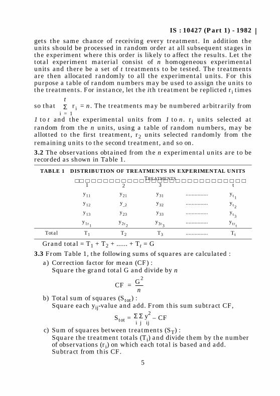
1 to t and the experimental units from 1 to n. ri units selected atrandom from the n units, using a table of random numbers, may beallotted to the first treatment, r2 units selected randomly from theremaining units to the second treatment, and so on.3.2 The observations obtained from the n experimental units are to berecorded as shown in Table 1.

Grand total = T1 + T2 + ...... + Tt = G

3.3 From Table 1, the following sums of squares are calculated :

TABLE 1 DISTRIBUTION OF TREATMENTS IN EXPERIMENTAL UNITSTREATMENTS

1 2 3 t

...............

...............

...............

...............

Total T1 T2 T3 ............... Tt

a) Correction factor for mean (CF) :Square the grand total G and divide by n

b) Total sum of squares (Stot) :Square each yij-value and add. From this sum subtract CF,

Stot = – CF

c) Sum of squares between treatments (ST) :Square the treatment totals (Ti) and divide them by the number of observations (ri) on which each total is based and add. Subtract from this CF.

tΣ

i 1=ri

y11 y21 y31 yt1y12 y_2 y32 yt2y13 y23 y33 yt3y1r1

y2r2y3r3

ytrt

CF G2

n-------=

Σ Σ y2

i j ij

IS : 10427 (Part 1) - 1982

6

d) Sum of squares due to experimental error (SE) :

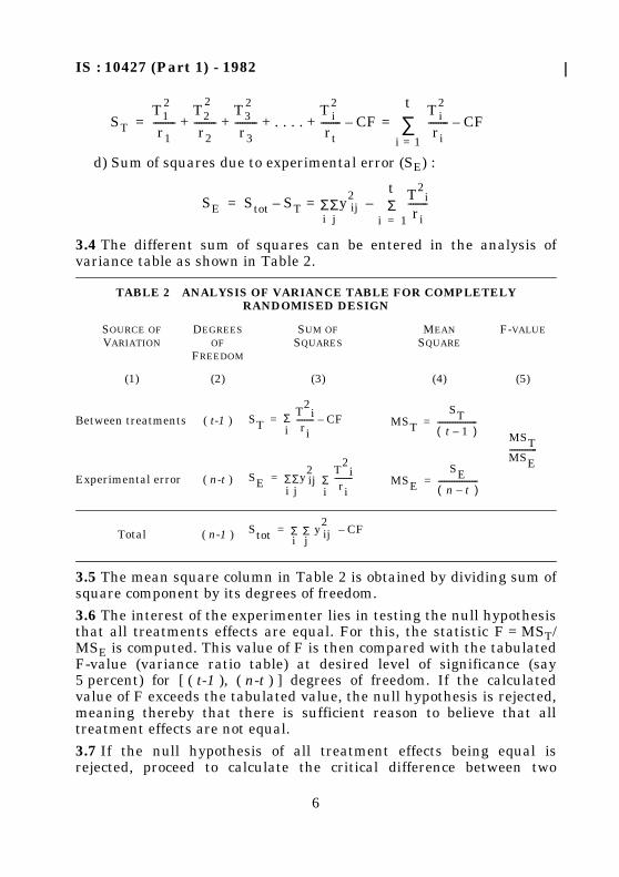
3.4 The different sum of squares can be entered in the analysis ofvariance table as shown in Table 2.

3.5 The mean square column in Table 2 is obtained by dividing sum ofsquare component by its degrees of freedom.

3.6 The interest of the experimenter lies in testing the null hypothesisthat all treatments effects are equal. For this, the statistic F = MST/MSE is computed. This value of F is then compared with the tabulatedF-value (variance ratio table) at desired level of significance (say5 percent) for [ ( t-1 ), ( n-t ) ] degrees of freedom. If the calculatedvalue of F exceeds the tabulated value, the null hypothesis is rejected,meaning thereby that there is sufficient reason to believe that alltreatment effects are not equal.

3.7 If the null hypothesis of all treatment effects being equal isrejected, proceed to calculate the critical difference between two

TABLE 2 ANALYSIS OF VARIANCE TABLE FOR COMPLETELY RANDOMISED DESIGN

SOURCE OFVARIATION

DEGREESOF

FREEDOM

SUM OFSQUARES

MEANSQUARE

F-VALUE

(1) (2) (3) (4) (5)

Between treatments ( t-1 )

Experimental error ( n-t )

Total ( n-1 )

STT1

2

r1---------

T22

r2---------

T32

r3--------- . . . .

T i2

rt-------- CF

i 1=

t

∑Ti

2

ri-------- CF–=–+ + + +=

SE Stot ST ΣiΣjy2

ij

tΣ

i 1=

T2i

ri--------–=–=

ST Σi T

2i

ri--------- CF–= MST

ST t 1 –( )

--------------------=MSTMSE--------------

SE ΣiΣjy

2ij Σ

i T

2i

ri---------= MSE

SE n t –( )

--------------------=

Stot Σi

Σj y

2ij CF–=

IS : 10427 (Part 1) - 1982

7

treatments. The critical difference between any two treatments, say tiand tj is given as follows :

Critical difference (CD) =

where tα is the α% value of t-variate with ( n-t ) degrees of freedom, αbeing the level of significance.

3.7.1 The mean for each treatment is then calculated as yi = Ti/ri.

3.7.2 The absolute difference between any two treatment means iscompared with its critical difference. If the difference between the twotreatment means is less than the critical difference, the twotreatments are not considered to be significantly different. If theabsolute difference between two treatment means is greater than thecritical difference, it is considered that these are significantly different.

3.8 Merits and Demerits

3.8.1 Merits

3.8.2 Demerits — As the experimental units are heterogeneous, theunits that receive one treatment may not be similar to those whichreceive another treatment and so the entire variation among the unitsenters into the experimental error. So the experimental error is higheras compared to other designs.

3.9 Complete randomisation is therefore only appropriate, wherea) the experimental units are homogeneous, andb) an appreciable fraction of the units is likely to be destroyed or fail

to respond.

3.10 Example 1 — Six hourly samples were taken from each of thethree different types of mixes during grinding of final cement fordetermination of rapid calcium oxide content. The test results of thesamples are given in Table 3. It has to be tested whether the differenttypes of mixes produce the same calcium oxide content.

a) It allows complete flexibility as any number of treatments andreplicates may be used. The number of replicates, if desired, canbe varied from treatment to treatment;

b) The statistical analysis is easy even if the number of replicatesare not the same for all treatments or if the experimental errorsdiffer from treatment to treatment; and

c) The relative loss of information due to missing observations issmaller than with any other design and they do not pose anyproblem in the analysis of data.

1ri---- 1

rj---- +

× MSE 12---

× tα

IS : 10427 (Part 1) - 1982

8

3.10.1 The various calculations are as given below:

3.10.2 The analysis of variance table for above experiment is given inTable 4.

3.10.3 The tabulated value of F at 5 percent level of significance, for(2,15) degrees of freedom is 3.68, which is less than the calculatedvalue. Hence the three different types of mixes are significantlydifferent, as far as calcium oxide content is concerned.

TABLE 3 CALCIUM OXIDE CONTENT (IN PERCENT)

( Clause 3.10 )

MIX I MIX II MIX III

(1) (2) (3)

43.9 45.0 44.244.0 45.1 44.443.9 45.1 44.144.0 45.2 44.043.9 45.0 44.244.1 45.0 44.1

Total 263.8 270.4 265.0, G = 799.2

a) Correction factor (CF) = = 35 484.48

b) Total sum of squares

= 4.28c) Sum of squares between mixes

d) Sum of squares due to error = 4.28 – 4.12 = 0.16

TABLE 4 ANALYSIS OF VARIANCE TABLE

SOURCE OFVARIATION

DEGREES OF FREEDOM

SUM OFSQUARES

MEANSQUARE

F-VALUE

(1) (2) (3) (4) (5)

Between mixes 2 4.12 2.06 187

Experimental error 15 0.16 0.011

Total 17 4.28

799.2( )2

18----------------------

43.9( )2 44.0( )2 ...... 44.1( )2+ + + ][ CF–=

263.8( )2

6---------------------- 270.4( )

6-------------------

2 265.0( )6

-------------------2

CF 4.12=–+ +=

IS : 10427 (Part 1) - 1982

9

3.10.4 The critical difference for different pairs is calculated next. Forinstance, the critical difference value at 5 percent level, for mixes Iand III is given by:

Critical difference (CD)

= 0.133.10.4.1 The average for mix I (y1) = 43.97 and for mix III (y3) = 44.17.Since | | (= 0.20) is greater than the critical difference value,mixes I and III are significantly different at 5 percent significancelevel.

4. RANDOMISED BLOCK DESIGN

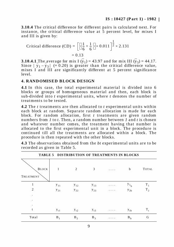
4.1 In this case, the total experimental material is divided into 6blocks or groups of homogeneous material and then, each block issub-divided into t experimental units, where t denotes the number oftreatments to be tested.4.2 The t treatments are then allocated to t experimental units withineach block at random. Separate random allocation is made for eachblock. For random allocation, first t treatments are given randomnumbers from 1 to t. Then, a random number between 1 and t is chosenand whatever number comes, the treatment having that number isallocated to the first experimental unit in a block. The procedure iscontinued till all the treatments are allocated within a block. Theprocedure is then repeated with the other blocks.4.3 The observations obtained from the bt experimental units are to berecorded as given in Table 5.

TABLE 5 DISTRIBUTION OF TREATMENTS IN BLOCKS

BLOCK 1 2 3 . . . . b TOTAL

TREATMENT

1 . . . .

2 . . . .

.

.

.

t . . . .

Total . . . . G

16--- 1

6--- +

× 0.01112---

× 2.131=

y1 y3–

y11 y12 y13y1b T1

y21 y22 y23 y2b T2

yt1 yt2 yt3 ytb Tt

B1 B2 B3 Bb

IS : 10427 (Part 1) - 1982

10

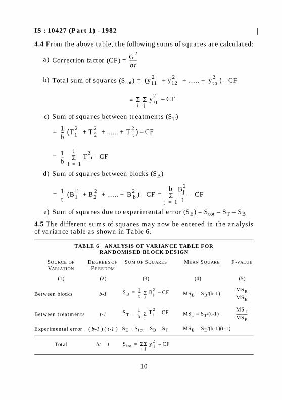
4.4 From the above table, the following sums of squares are calculated:

4.5 The different sums of squares may now be entered in the analysisof variance table as shown in Table 6.

a) Correction factor (CF) =

b) Total sum of squares (Stot)

c) Sum of squares between treatments (ST)

d) Sum of squares between blocks (SB)

e) Sum of squares due to experimental error (SE) = Stot – ST – SB

TABLE 6 ANALYSIS OF VARIANCE TABLE FORRANDOMISED BLOCK DESIGN

SOURCE OFVARIATION

DEGREES OF FREEDOM

SUM OF SQUARES MEAN SQUARE F-VALUE

(1) (2) (3) (4) (5)

Between blocks b-1 MSB = SB/(b-1)

Between treatments t-1 MST = ST/(t-1)

Experimental error ( b-1 ) ( t-1 ) SE = Stot – SB – ST MSE = SE/(b-1)(t-1)

Total bt – 1

G2

bt-------

y112 y12

2 ...... ytb2+ + +( ) CF–=

Σ=i Σj

y2ij CF–

1b--- T1

2( T 22 ...... T t

2 ) CF–+ + +=

1b---

tΣ

i 1= T2

i CF–=

1t--- B1

2B2

2 ...... B b2+ + +( ) CF

bΣ

j 1=

Bj2

t-------- CF–=–=

SB1t--- Σ

j Bj

2 CF–= MSB

MSE------------

ST1b--- Σ

i Ti

2 CF–= MST

MSE------------

Stot ΣiΣj yjj

2 CF–=

IS : 10427 (Part 1) - 1982

11

4.6 Since the interest of the experimental lies in testing the hypothesiswhether all treatment effects are identical, the following statistic iscomputed :

F = MST/MSE

4.6.1 The calculated value of F is then compared with the tabulatedF-value (variance ratio table) at desired level of significance (say5 percent) for [ ( t-1 ), ( b-1 ) ( t-1 ) ] degrees of freedom. If thecalculated value of F is less than the tabulated value, the nullhypothesis is not rejected meaning thereby that there is no significantdifference among treatments. If the calculated value of F exceeds thetabulated value, reject the null hypothesis meaning thereby that thereis sufficient reason to believe that all treatment effects are not equal.


4.7.1 Merits

4.7.2 Demeritsa) The effect of only one factor is investigated, andb) Single grouping of only one factor yields higher experimental

error as compared to more complicated designs.

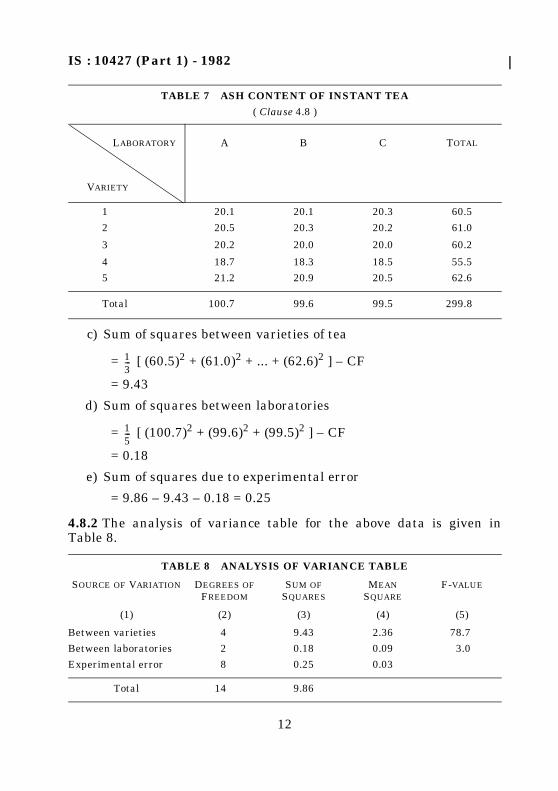
4.8 Example — An experiment was conducted for ash content ofinstant tea. For this purpose five different varieties of instant tea weretested in three laboratories. The test results are given in Table 7. Ithas to be determined whether there is significant difference amongvarieties of instant tea.

4.8.1 The various calculations are obtained as follows:


b) Total sum of squares =

[(20.1)2 + (20.1)2 + ... + (20.5)2] – CF = 9.86

a) By means of grouping, the experimental error is reduced and thetreatment comparisons are made more sensitive than withcompletely randomised designs;

b) Any number of treatments and replicates may be included.However, if the number of treatments is large (20 or more), theefficiency of error control decreases; and

c) The statistical analysis is straightforward. When data from someindividual units are missing, the ‘missing plot’ technique enablesthe available results to be fully utilized.

299.8( )2

15----------------------

IS : 10427 (Part 1) - 1982

12

4.8.2 The analysis of variance table for the above data is given inTable 8.

TABLE 7 ASH CONTENT OF INSTANT TEA

( Clause 4.8 )

LABORATORY A B C TOTAL

VARIETY

1 20.1 20.1 20.3 60.5

2 20.5 20.3 20.2 61.0

3 20.2 20.0 20.0 60.2

4 18.7 18.3 18.5 55.5

5 21.2 20.9 20.5 62.6

Total 100.7 99.6 99.5 299.8

c) Sum of squares between varieties of tea

= [ (60.5)2 + (61.0)2 + ... + (62.6)2 ] – CF

= 9.43

d) Sum of squares between laboratories

= [ (100.7)2 + (99.6)2 + (99.5)2 ] – CF

= 0.18

e) Sum of squares due to experimental error

= 9.86 – 9.43 – 0.18 = 0.25


SOURCE OF VARIATION DEGREES OF FREEDOM

SUM OFSQUARES

MEANSQUARE

F-VALUE

(1) (2) (3) (4) (5)

Between varieties 4 9.43 2.36 78.7

Between laboratories 2 0.18 0.09 3.0


Total 14 9.86

13---

15---

IS : 10427 (Part 1) - 1982

13

4.8.3 The tabulated value of F for (4, 8) degrees of freedom at 5 percentsignificance level is 3.84, which is less than the calculated F-value of78.7. So it can be concluded that there is significant difference amongthe varieties of instant tea.

5. LATIN SQUARE DESIGN

5.1 In the latin square design, the treatments are classified incomplete groups in two directions, the two classifications beingorthogonal to each other and also to the treatments. Each row and eachcolumn is a complete replication. The effect of the double grouping is toeliminate from the errors, all differences among rows, as also all thedifferences among columns. The experimental material should bearranged and the experiment conducted so that the differences amongrows and columns represent major sources of variation.

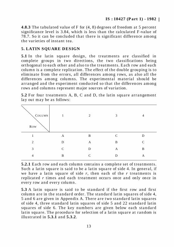
5.2 For four treatments A, B, C and D, the latin square arrangementlay out may be as follows:

5.2.1 Each row and each column contains a complete set of treatments.Such a latin square is said to be a latin square of side 4. In general, ifwe have a latin square of side r, then each of the r treatments isreplicated r times and each treatment occurs once and only once inevery row and every column.

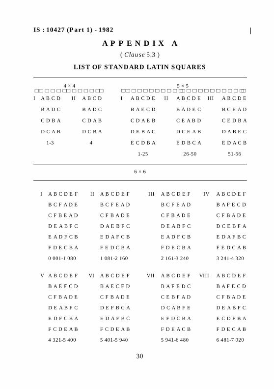
5.3 A latin square is said to be standard if the first row and firstcolumn are in the standard order. The standard latin squares of side 4,5 and 6 are given in Appendix A. There are two standard latin squaresof side 4, three standard latin squares of side 5 and 22 standard latinsquares of side 6. The key numbers are given below each standardlatin square. The procedure for selection of a latin square at random isillustrated in 5.3.1 and 5.3.2.

COLUMN 1 2 3 4

ROW

1 A B C D

2 D A B C

3 C D A B

4 B C D A

IS : 10427 (Part 1) - 1982

14

5.3.1 If 5 × 5 latin square is required, it can be seen by referring toAppendix A, that the largest key number for 5 × 5 latin square is 56.Hence a random number from 1 to 56 is chosen. Let the randomnumber chosen be 18. Since 18 is in the range of key numbers 1 to 25,standard latin square number 1 is selected. Next, all the rows of theselected standard latin square are permuted at random by selectingthe digits from 1 to 5 from the random number tables given inIS : 4905-1968*. The procedure of selection of digits at random is givenin 4.2 of IS : 4905-1968*. Let, for example, the order of digits obtainedat random be 4, 3, 1, 5 and 2. This implies that fourth row shall be thefirst row, the third row shall come next and so on. After permuting therows and random, all the columns are permuted at random in thesame way. The letters to the treatments are then assigned at random.

5.3.2 For latin squares of sides 7 to 10, one square for each side isgiven in Appendix A, from which any square of the transformation setsmay be generated by the random permutation of all rows and columns.The letters to the treatments are then assigned at random. Therandom permutation may be done as in 5.3.1.

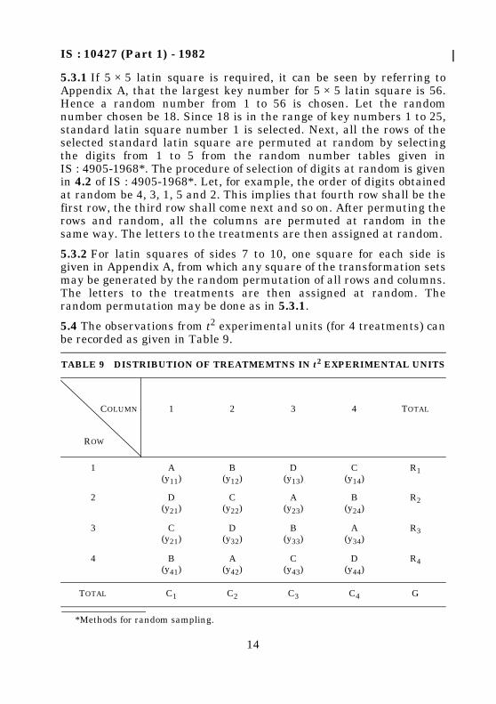
5.4 The observations from t2 experimental units (for 4 treatments) canbe recorded as given in Table 9.

*Methods for random sampling.

TABLE 9 DISTRIBUTION OF TREATMEMTNS IN t2 EXPERIMENTAL UNITS

COLUMN 1 2 3 4 TOTAL

ROW

1 A(y11)

B(y12)

D(y13)

C(y14)

R1

2 D(y21)

C(y22)

A(y23)

B(y24)

R2

3 C(y21)

D(y32)

B(y33)

A(y34)

R3

4 B(y41)

A(y42)

C(y43)

D(y44)

R4

TOTAL C1 C2 C3 C4 G

IS : 10427 (Part 1) - 1982

15

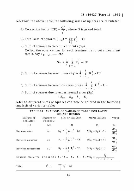
5.5 From the above table, the following sums of squares are calculated:

5.6 The different sums of squares can now be entered in the followinganalysis of variance table:

a) Correction factor (CF) = , where G is grand total.

b) Total sum of squares (Stot)

c) Sum of squares between treatments (ST) :Collect the observations for each treatment and get t treatmenttotals, say T1, T2......... etc.

d) Sum of squares between rows (SR) =

e) Sum of squares between columns (SC) =

f) Sum of squares due to experimental error (SE)= Stot – SR – SC – ST

TABLE 10 ANALYSIS OF VARIANCE TABLE FOR LATINSQUARE DESIGN

SOURCE OFVARIATION

DEGREES OF FREEDOM


(1) (2) (3) (4) (5)

Between rows t-1 MSR = SR/( t-1 )

Between columns t-1 MSC = SC/( t-1 )

Between treatments t-1 MST = ST/( t-1 )

Experimental error ( t-1 ) ( t-2 ) SE = Stot – SR – SC – ST MSE =

Total t2 - 1

G2

t2-------

ΣiΣj yij

2 CF–=

ST1t---

tΣ

i 1=Ti

2 CF–=

1t---

tΣ

i 1=R i

2 CF–

1t---

tΣ

i 1=Ci

2 CF–

SR1t--- Σ

i Ri

2 CF–=MSR

MSE------------

SC1t--- Σ

i Ci

2 CF–=MSC

MSE------------

ST1t--- Σ

i Ti

2 CF–=MST

MSE------------

SE

t 1 –( ) t 2 –( )-------------------------------------------

ΣiΣj yij

2 CF–

IS : 10427 (Part 1) - 1982

16

5.7 For testing the differences between treatments or rows or columns,the mean square for that particular component is compared with themean square due to experimental error, that is,

F1 = MST/MSE, F2 = MSR/MSE and F3 = MSC/MSE

5.7.1 If the computed value of F1, (say) exceeds the tabulated value ofF at desired level of significance for [ ( t-1 ), ( t-1 ) ( t-2 ) ] degrees offreedom, the hypothesis that all treatment effects are equal is rejected.The next step is to calculate the critical differences in a similar fashionas given in 4.7.


5.8.1 Meritsa) More than one factor can be investigated simultaneously and

with fewer replications than more complicated designs, andb) Due to double grouping, latin square provides more opportunity

than randomised block design for the reduction of errors.

5.8.2 Demeritsa) The design has a restriction that each treatment may occur only

once in each row and each column,b) An assumption is made that the factors are independent, andc) Latin square is not suitable when the number of treatments is

large as there will be as many replications as there aretreatments. Moreover, when there are more treatments, it may bedifficult to allocate the rows and the columns to sources ofvariability in an efficient manner.

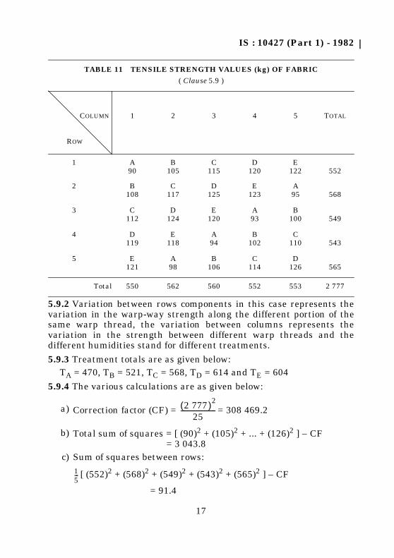
5.9 Example 3 — In order to study the effect of relative humidity (RH)on the warp-way tensile strength of a standard hessian fabric, one3 × 1.5 m fabric sample was cut from a 100 × 1.5 m hessian of the abovetype. Twenty-five fabric test specimens each of dimension 10 × 20 cmwere then cut from five different rows of the fabric sample, each rowcontaining five test specimen. In each row, five specimen were testedunder five different relative humidities. So at each relative humidity,five strength tests were carried out. The plan of selecting the testspecimens and the test results (kg) obtained are as given in Table 11.

5.9.1 In Table 11, each cell may be considered as a test specimen ofdimension 10 × 20 cm. The alphabet within a cell represents thehumidity at which the test specimen is tested, while the numericalvalue appearing at the bottom within the same cell represents thestrength value (kg) obtained at the particular humidity.

IS : 10427 (Part 1) - 1982

17

5.9.2 Variation between rows components in this case represents thevariation in the warp-way strength along the different portion of thesame warp thread, the variation between columns represents thevariation in the strength between different warp threads and thedifferent humidities stand for different treatments.

5.9.3 Treatment totals are as given below:TA = 470, TB = 521, TC = 568, TD = 614 and TE = 604


TABLE 11 TENSILE STRENGTH VALUES (kg) OF FABRIC

( Clause 5.9 )

COLUMN 1 2 3 4 5 TOTAL

ROW

1 A90

B105

C115

D120

E122 552

2 B108

C117

D125

E123

A95 568

3 C112

D124

E120

A93

B100 549

4 D119

E118

A94

B102

C110 543

5 E121

A98

B106

C114

D126 565

Total 550 562 560 552 553 2 777


b) Total sum of squares = [ (90)2 + (105)2 + ... + (126)2 ] – CF= 3 043.8

c) Sum of squares between rows:

[ (552)2 + (568)2 + (549)2 + (543)2 + (565)2 ] – CF

= 91.4

2 777( )2

25----------------------

15---

IS : 10427 (Part 1) - 1982

18

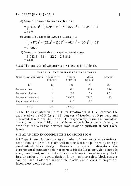
5.9.5 The analysis of variance table is given in Table 12.

5.9.6 The calculated value of F for treatments is 195, whereas thetabulated value of F for (4, 12) degrees of freedom at 5 percent and1 percent levels are 3.26 and 5.41 respectively. Thus the variationamong treatments is highly significant at both these levels. It may beseen that the variation between rows is also significant at both theselevels.

6. BALANCED INCOMPLETE BLOCK DESIGN

6.1 Experiments for comparing a number of treatments when uniformconditions can be maintained within blocks can be planned by using arandomised block design. However, in certain situations theexperimental conditions do not permit blocks large enough to includeevery treatment, so that not all treatments are included in every block.In a situation of this type, designs known as incomplete block designscan be used. Balanced incomplete blocks are a class of importantincomplete block designs.

d) Sum of squares between columns :

= [ (550)2 + (562)2 + (560)2 + (552)2 + (553)2 ] – CF

= 22.2e) Sum of squares between treatments:

= [ (470)2 + (521)2 + (568)2 + (614)2 + (604)2 ] – CF

= 2 886.2f) Sum of squares due to experimental error

= 3 043.8 – 91.4 – 22.2 – 2 886.2= 44.0


SOURCES OF VARIATION DEGREES OF FREEDOM

SUM OFSQUARES

MEANSQUARE

F-VALUE

(1) (2) (3) (4) (5)

Between rows 4 91.4 22.8 6.16

Between columns 4 22.2 5.6 1.51

Between treatments 4 2 886.2 721.5 195

Experimental Error 12 44.0 3.7

Total 24 3 043.8

15---

15---

IS : 10427 (Part 1) - 1982

19

6.2 In a balanced incomplete block (BIB) design, the experimentalmaterial is divided into ‘b’ blocks of ‘k’ units each ( k < t ), where t isthe total number of treatments to be tested. Each treatment isreplicated ‘r’ times, that is, the treatments are so arranged that eachtreatment occurs in exactly ‘r’ blocks and further, each pair oftreatment occurs together in ‘λ’ blocks. The integers t, b, r, k and λ arecalled the parameters of the design. The constraints on the parametersof the design are as follows:

a) t > k,b) tr = bk, andc) λ (t-1) = r(k-1)

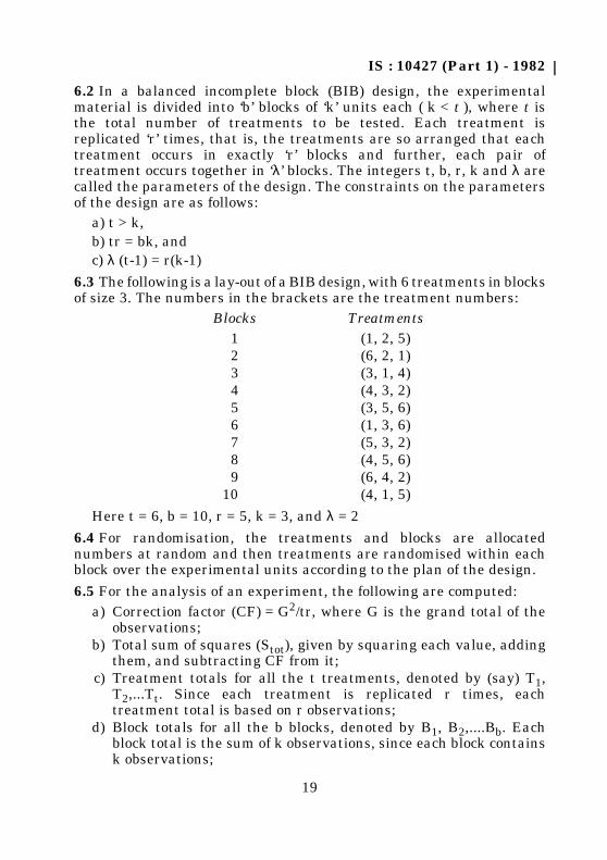
6.3 The following is a lay-out of a BIB design, with 6 treatments in blocksof size 3. The numbers in the brackets are the treatment numbers:

Here t = 6, b = 10, r = 5, k = 3, and λ = 2

6.4 For randomisation, the treatments and blocks are allocatednumbers at random and then treatments are randomised within eachblock over the experimental units according to the plan of the design.

6.5 For the analysis of an experiment, the following are computed:

Blocks Treatments1 (1, 2, 5)2 (6, 2, 1)3 (3, 1, 4)4 (4, 3, 2)5 (3, 5, 6)6 (1, 3, 6)7 (5, 3, 2)8 (4, 5, 6)9 (6, 4, 2)

10 (4, 1, 5)

a) Correction factor (CF) = G2/tr, where G is the grand total of theobservations;

b) Total sum of squares (Stot), given by squaring each value, addingthem, and subtracting CF from it;

c) Treatment totals for all the t treatments, denoted by (say) T1,T2,...Tt. Since each treatment is replicated r times, eachtreatment total is based on r observations;

d) Block totals for all the b blocks, denoted by B1, B2,....Bb. Eachblock total is the sum of k observations, since each block containsk observations;

IS : 10427 (Part 1) - 1982

20

.

.

.

In the above expressions, the sum Bj denotes the sum of all those

block totals which contain the i = th treatment. It may be verified that∑Qi = 0. For instance, in 6.3 the various adjusted totals are:

Q1 = T1 – ( B1 + B2 + B3 + B6 + B10 )

Q2 = T2 – ( B1 + B2 + B4 + B7 + B9 )

Q3 = T3 – ( B3 + B4 + B5 + B6 + B7 )

Q4 = T4 – ( B3 + B4 + B8 + B9 + B10 )

Q5 = T5 – ( B1 + B5 + B7 + B8 + B10 )

Q6 = T6 – ( B2 + B5 + B6 + B8 + B9 )Therefore ∑Qi = 0

e) Adjusted treatment totals denoted by Q1, Q2 .... Qt for all thetreatments are given by subtracting from the treatment total theratio of the block totals where the particular treatment occurs, tothe number of units in each blocks,

f) Efficiency factor (E) = λt/rkNOTE — The efficiency factor measures the efficiency of balanced incompleteblock design over randomised block design.

g) Adjusted treatment sum of squares (S'T) is given by:

h) The sum of squares (unadjusted) for blocks is given by:

j) The sum of squares (unadjusted) for treatments is given by:

Q1 T11k--- Σ

j (1)Bj–=

Q2 T21k--- Σ

j (2)Bj–=

Qt Tt1k--- Σ

j (t)Bj–=

Σj (i)

13---

13---

13---

13---

13---

13---

S'Tkλt----- Q1

2 Q22 ...... Qt

2+ +( )=

SB1k--- B1

2 B22 ...... Bb

2+ + +( ) CF–=

ST1r--- T1

2 T22

......+ Tt2+ +( ) CF–=

IS : 10427 (Part 1) - 1982

21

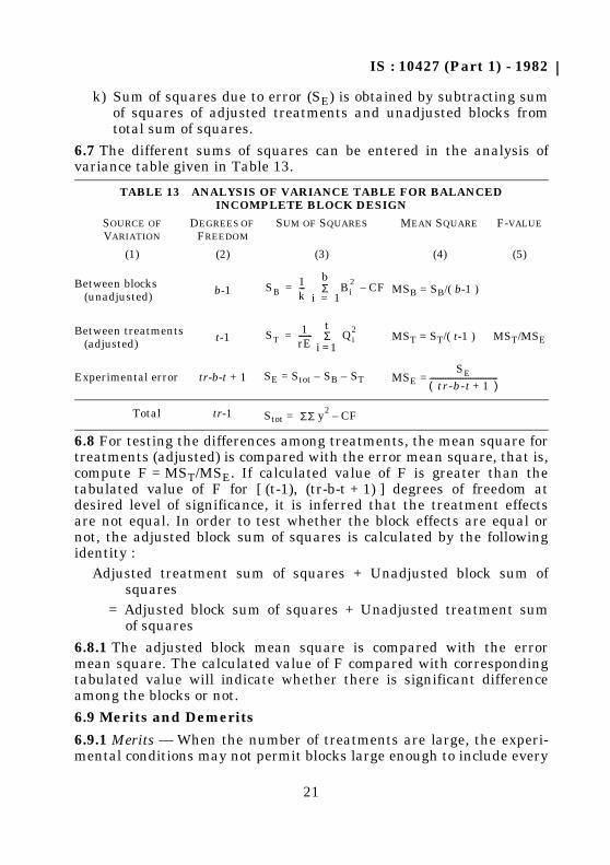
6.7 The different sums of squares can be entered in the analysis ofvariance table given in Table 13.

6.8 For testing the differences among treatments, the mean square fortreatments (adjusted) is compared with the error mean square, that is,compute F = MST/MSE. If calculated value of F is greater than thetabulated value of F for [ (t-1), (tr-b-t + 1) ] degrees of freedom atdesired level of significance, it is inferred that the treatment effectsare not equal. In order to test whether the block effects are equal ornot, the adjusted block sum of squares is calculated by the followingidentity :

Adjusted treatment sum of squares + Unadjusted block sum ofsquares

= Adjusted block sum of squares + Unadjusted treatment sumof squares

6.8.1 The adjusted block mean square is compared with the errormean square. The calculated value of F compared with correspondingtabulated value will indicate whether there is significant differenceamong the blocks or not.


6.9.1 Merits — When the number of treatments are large, the experi-mental conditions may not permit blocks large enough to include every

k) Sum of squares due to error (SE) is obtained by subtracting sumof squares of adjusted treatments and unadjusted blocks fromtotal sum of squares.

TABLE 13 ANALYSIS OF VARIANCE TABLE FOR BALANCEDINCOMPLETE BLOCK DESIGN

SOURCE OFVARIATION

DEGREES OF FREEDOM


(1) (2) (3) (4) (5)

Between blocks(unadjusted) b-1 MSB = SB/( b-1 )

Between treatments(adjusted) t-1 MST = ST/( t-1 ) MST/MSE

Experimental error tr-b-t + 1 SE = Stot – SB – ST MSE =

Total tr-1 Stot =

SB1k---

bΣ

i 1=Bi

2 CF–=

ST1

rE-------

tΣ

i 1=Qi

2=

SE

tr-b-t 1 +( )-----------------------------------

ΣΣ y2 CF–

IS : 10427 (Part 1) - 1982

22

treatment, so that all the treatments cannot be tested under uniformconditions. In such cases the designs discussed earlier in this standardcan not be applied and balanced incomplete blocks designs are used.

6.9.2 Demerits

a) The analysis of balanced incomplete block designs is morecomplicated as compared to other designs.

b) This design has many constraints, like tr = bk, λ (t-1) = r (k-1).Therefore theoretically it may be possible to construct BIBD for agiven value of k and t, but most of these are of little use inpractice because it will require large value of ‘r’.

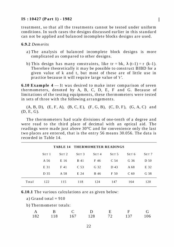
6.10 Example 4 — It was desired to make inter comparison of seventhermometers, denoted by A, B, C, D, E, F and G. Because oflimitations of the testing equipments, these thermometers were testedin sets of three with the following arrangements.

(A, B, D), (E, F, A), (B, C, E), (F, G, B), (C, D, F), (G, A, C) and(D, E, G).

The thermometers had scale divisions of one-tenth of a degree andwere read to the third place of decimal with an optical aid. Thereadings were made just above 30°C and for convenience only the lasttwo places are entered, that is the entry 56 means 30.056. The data isrecorded in Table 14.


a) Grand total = 910

b) Thermometer totals:

TABLE 14 THERMOMETER READINGS

SET 1 SET 2 SET 3 SET 4 SET 5 SET 6 SET 7

A 56 E 16 B 41 F 46 C 54 G 36 D 50

E 31 F 41 C 53 G 32 D 43 A 68 E 32

D 35 A 58 E 24 B 46 F 50 C 60 G 38

Total 122 115 118 124 147 164 120

A182

B118

C167

D128

E72

F137

G106

IS : 10427 (Part 1) - 1982

23

c) Adjusted totals ( Qi ) :

d) Adjusted sum of squares for thermometers =

Here r = 3, E = = = 7/9; thus rE = 7/3.

Adjusted sum of squares for thermometers

= (5 980.771 2) = 2 563.19

e) Correction factor = = 39 433.33

f) Unadjusted sum of squares for sets

= [ (122)2 + (115)2 + ... + (120)2 ] – CF

= 671.33g) Total sum of squares = 42 698 – CF = 3 264.67h) Error sum of squares = 3 264.67 – 2 563.19 – 671.33 = 30.15j) Unadjusted sum of squares between thermometers

= [ (182)2 + (118)2 + ... (106)2 ] – CF = 2 736.67k) Adjusted sum of squares for sets = 671.33 + 2 563.19 – 2 736.67

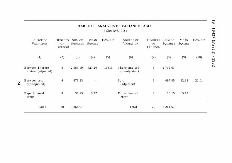
= 497.856.10.2 The analysis of variance table is given in Table 15.

6.10.3 The tabulated value of F for (6, 8) degrees of freedom and at 5percent level is 3.58. Thus, the thermometers and sets can be regardedas significantly different.

7. FACTORIAL EXPERIMENTS

7.1 The testing of a number of treatments, not necessarily related to eachother have been discussed earlier in randomised blocks, and latin squaredesigns. However, in industrial applications, several factors may affectthe characteristic under study and it is intended to estimate the effectof each of the factors and how the effect of one factor varies over the levelsof the other factors. In such situation, the logical procedure would be tovary all factors simultaneously within the framework of the sameexperiment. Such experiments are known as factorial experiments.

QA48.33

QB– 3.33

QC24.00

QD– 1.66

QE– 45.67

QF8.33

QG– 30.00

Σi Qi

2

rE---------------

λtrk------ 1 × 7

3 × 3-------------

37--- QA

2 QB2 ... QG

2+ + +( )=

37---

910( )2

21-----------------

13---

13---

IS:10427

(Pa

rtI)

-1982

24


( Clause 6.10.2 )

SOURCE OF VARIATION

DEGREES OF

FREEDOM

SUM OFSQUARES

MEANSQUARE

F-VALUE SOURCE OF VARIATION

DEGREES OF

FREEDOM

SUM OFSQUARES

MEANSQUARE

F-VALUE

(1) (2) (3) (4) (5) (6) (7) (8) (9) (10)

Between Thermo- meters (adjusted)

6 2 563.19 427.20 113.3 Thermometers (unadjusted)

6 2 736.67 —

Between sets (unadjusted)

6 671.33 — Sets(adjusted)

6 497.85 82.98 22.01

Experimentalerror

8 30.15 3.77 Experimentalerror

8 30.15 3.77

Total 20 3 264.67 Total 20 3 264.67

IS : 10427 (Part 1) - 1982

25

7.2 The factorial experiments are particularly useful in experimentalsituations which require the examination of the effects of varying twoor more factors. In such situations, it is not sufficient to vary one factorat a time; all combinations of the different factor levels must beexamined in order to elucidate the effect of each factor and the possibleways in which each factor may be modified by the variation of theothers. In the analysis of the experimental results, the effect of eachfactor can be determined with the same accuracy as if only one factorhad been varied at a time and the interaction effects between thefactors can also be evaluated.7.3 Designs with Factors at Two Levels (2n Series) — Thesimplest class of factorial experiment is that involving factors at twolevels, that is, the 2n series, n being the number of factors examined inthe experiment. The notations being used in the 2n designs by Yates,and the calculations of main effects and the interactions are as givenin 7.3.1 to 7.3.3.7.3.1 Notation — The letters A, B, C ... denote the factors and thelevels of A, B, C ... are denoted by (1), a; (1), b; (1), c; ... respectively. Asa convention, the lower case letters a, b, c ... denote the higher levels ofthe factors. The low level is signified by the absence of thecorresponding letter. Thus the treatment combination bd, in a 24

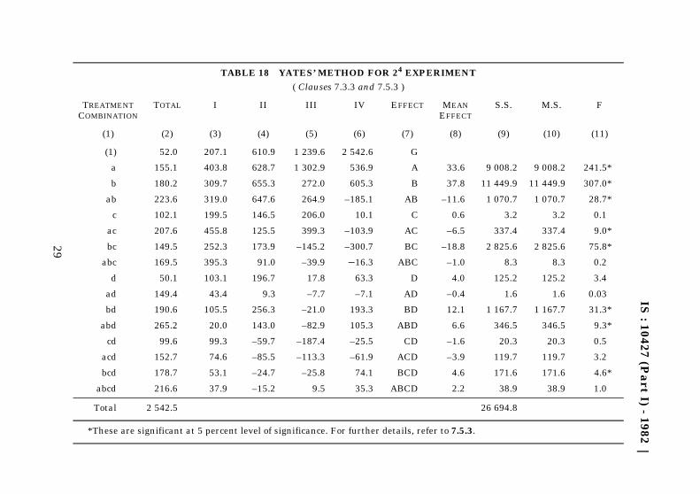
factorial experiment, means the treatment combination which containsthe first (low) level of factor A and C, and the second (high) level offactors B and D. The treatment combination which consists of the firstlevel of all factors is denoted by the symbol (1). The letters A, B, C, AB,when they refer to numbers, represent respectively the main effects offactors A, B, C and the interaction effect of factors A and B respectively.7.3.2 Main Effects and Interactions — The change in the averageresponse produced by a change in the level of the factor is called its“main effect.” It may so happen sometimes that the effect of one factoris different at different levels of one or more of the other factors, in thiscase the two factors are said to interact each other. The interactionbetween two factors is termed as “First order interaction”, or “Twofactor interaction” and is denoted by AB. If the interaction between twofactors AB is different at different levels of a third factor C, then thereis said to be an interaction between the three factors. This is referred toas ‘second order interaction’ or ‘three factor interaction’ and is denotedby ABC. Similarly the third and higher order interactions are defined.7.3.3 Yates has developed a systematic tabular method for calculationof main effects and interaction for 2n factorial experiment. The varioussteps in the computation are explained below with the help of Table 18.

a) Arrange the treatment combinations in standard order as shownin Column 1 titled ‘treatment combinations’.

IS : 10427 (Part 1) - 1982

26

7.4 Merits and Demerits7.4.1 Merits

7.4.2 Demeritsa) The experiment can be too large when all combinations of factors

and levels are run, andb) The size of the experiment requires a larger amount of homo-

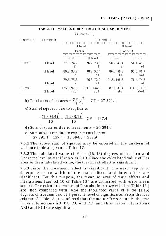
geneous material than other designs.7.5 Example — In an experiment, four factors A, B, C, and D each attwo levels are studied. The response obtained for each treatmentcombinations corresponding to two replicates is given in Table 16.Determine with the help of a factorial experiment as to which of themain effects and interactions are significant.

The various calculations are as given below :

a) Correction factor = = 202 009.6

b) Place the sum of values of each of the treatment combinations(from Table 16) in the second column titled ‘Total’.

c) Derive the top half of the third column titled ‘I’ by adding thevalues in pairs from the second column. The lower half of thiscolumn is obtained by taking the difference of same pairs, thefirst value of each pair being subtracted from the second value.

d) By the procedure given in (c), columns 4, 5 and 6 titled as II, IIIand IV are obtained from the columns 3, 4 and 5 respectively.

e) Repeat the procedure n times, where n is the number of factorsinvolved in the experiment. For Table 18, the procedure has beenrepeated 4 times thereby obtaining columns titled I to IV.

f) Obtain the mean factorial effect by dividing the total factorialeffect by r.2n–1 where r is the number of replicates. Column 8 isobtained by dividing each value of column 6 by 16 ( = 2 × 23 ).

g) The sum of squares due to different treatment combinations ofthe factorial effects (main effects and inter-actions) are obtainedby dividing the squares of the factorial effects total by r.2n.Column 9 is obtained by dividing the square of each value ofcolumn 6 by 32 ( = 2 × 24 ). The mean squares ( see column 10 ) issame as sum of squares, as the degrees of freedom for eachfactorial effect is one.

a) This design makes maximum utilization of all results and everyresult is used to evaluate each factor,

b) It can measure interaction of factors,c) The experimental error tends to be lower than other designs, andd) The final calculations have broader applicability because of scope

of experimental trials.

2 542.5( )2

32---------------------------

IS : 10427 (Part 1) - 1982

27

b) Total sum of squares = – CF = 27 391.1

c) Sum of squares due to replicates

d) Sum of squares due to treatments = 26 694.8e) Sum of squares due to experimental error

= 27 391.1 – 137.4 – 26 694.8 = 558.9

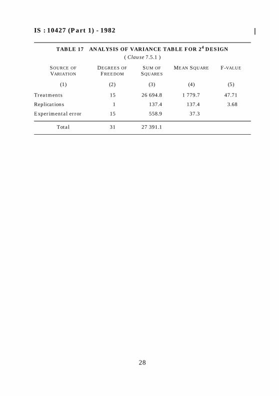
7.5.1 The above sum of squares may be entered in the analysis ofvariance table as given in Table 17.

7.5.2 The tabulated value of F for (15, 15) degrees of freedom and5 percent level of significance is 2.40. Since the calculated value of F isgreater than tabulated value, the treatment effect is significant.

7.5.3 Since the treatment effect is significant, the next step is todetermine as to which of the main effects and interactions aresignificant. For this purpose, the mean squares of main effects andinteractions ( see col 10 of Table 18 ) are compared with error meansquare. The calculated values of F so obtained ( see col 11 of Table 18 )are then compared with, 4.54 the tabulated value of F for (1,15)degrees of freedom and at 5 percent level of significance. From the lastcolumn of Table 18, it is inferred that the main effects A and B, the twofactor interactions AB, BC, AC and BD; and three factor interactionsABD and BCD are significant.

TABLE 16 VALUES FOR 24 FACTORIAL EXPERIMENT

( Clause 7.5 )

FACTOR A FACTOR B FACTOR C

I level II level

Factor D Factor D

I level II level I level II level

I level I level 27.3, 24.7(1)

26.2, 23.9d

58.7, 43.4c

50.1, 49.5cd

II level 86.3, 93.9b

98.2, 92.4bd

80.2, 69.3bc

92.0, 86.7bcd

I level79.6, 75.5

a76.5, 72.9

ad101.8, 105.8

ac78.4, 74.3

acd

II levelII level

125.8, 97.8ab

130.7, 134.5abd

82.1, 87.4abc

110.5, 106.1abcd

ΣiΣj yij

2

1 304.4( )2

16---------------------------= 1 238.1( )2

16--------------------------- CF 137.4=–+

IS : 10427 (Part 1) - 1982

28

TABLE 17 ANALYSIS OF VARIANCE TABLE FOR 24 DESIGN

( Clause 7.5.1 )

SOURCE OFVARIATION

DEGREES OF FREEDOM

SUM OFSQUARES

MEAN SQUARE F-VALUE

(1) (2) (3) (4) (5)

Treatments 15 26 694.8 1 779.7 47.71

Replications 1 137.4 137.4 3.68


Total 31 27 391.1

IS:10427

(Pa

rtI)

-1982

29

TABLE 18 YATES’ METHOD FOR 24 EXPERIMENT

( Clauses 7.3.3 and 7.5.3 )

TREATMENT COMBINATION

TOTAL I II III IV EFFECT MEAN EFFECT

S.S. M.S. F

(1) (2) (3) (4) (5) (6) (7) (8) (9) (10) (11)

(1) 52.0 207.1 610.9 1 239.6 2 542.6 G

a 155.1 403.8 628.7 1 302.9 536.9 A 33.6 9 008.2 9 008.2 241.5*

b 180.2 309.7 655.3 272.0 605.3 B 37.8 11 449.9 11 449.9 307.0*

ab 223.6 319.0 647.6 264.9 –185.1 AB –11.6 1 070.7 1 070.7 28.7*

c 102.1 199.5 146.5 206.0 10.1 C 0.6 3.2 3.2 0.1

ac 207.6 455.8 125.5 399.3 –103.9 AC –6.5 337.4 337.4 9.0*

bc 149.5 252.3 173.9 –145.2 –300.7 BC –18.8 2 825.6 2 825.6 75.8*

abc 169.5 395.3 91.0 –39.9 –16.3 ABC –1.0 8.3 8.3 0.2

d 50.1 103.1 196.7 17.8 63.3 D 4.0 125.2 125.2 3.4

ad 149.4 43.4 9.3 –7.7 –7.1 AD –0.4 1.6 1.6 0.03

bd 190.6 105.5 256.3 –21.0 193.3 BD 12.1 1 167.7 1 167.7 31.3*

abd 265.2 20.0 143.0 –82.9 105.3 ABD 6.6 346.5 346.5 9.3*

cd 99.6 99.3 –59.7 –187.4 –25.5 CD –1.6 20.3 20.3 0.5

acd 152.7 74.6 –85.5 –113.3 –61.9 ACD –3.9 119.7 119.7 3.2

bcd 178.7 53.1 –24.7 –25.8 74.1 BCD 4.6 171.6 171.6 4.6*

abcd 216.6 37.9 –15.2 9.5 35.3 ABCD 2.2 38.9 38.9 1.0

Total 2 542.5 26 694.8

*These are significant at 5 percent level of significance. For further details, refer to 7.5.3.

IS : 10427 (Part 1) - 1982

30

A P P E N D I X A( Clause 5.3 )

LIST OF STANDARD LATIN SQUARES

4 × 4 5 × 5

I A B C D II A B C D I A B C D E II A B C D E III A B C D E

B A D C B A D C B A E C D B A D E C B C E A D

C D B A C D A B C D A E B C E A B D C E D B A

D C A B D C B A D E B A C D C E A B D A B E C

1-3 4 E C D B A E D B C A E D A C B

1-25 26-50 51-56

6 × 6

I A B C D E F II A B C D E F III A B C D E F IV A B C D E F

B C F A D E B C F E A D B C F E A D B A F E C D

C F B E A D C F B A D E C F B A D E C F B A D E

D E A B F C D A E B F C D E A B F C D C E B F A

E A D F C B E D A F C B E A D F C B E D A F B C

F D E C B A F E D C B A F D E C B A F E D C A B

0 001-1 080 1 081-2 160 2 161-3 240 3 241-4 320

V A B C D E F VI A B C D E F VII A B C D E F VIII A B C D E F

B A E F C D B A E C F D B A F E D C B A F E C D

C F B A D E C F B A D E C E B F A D C F B A D E

D E A B F C D E F B C A D C A B F E D E A B F C

E D F C B A E D A F B C E F D C B A E C D F B A

F C D E A B F C D E A B F D E A C B F D E C A B

4 321-5 400 5 401-5 940 5 941-6 480 6 481-7 020

IS : 10427 (Part 1) - 1982

31

IX A B C D E F X A B C D E F XI A B C D E F XII A B C D E F

B C D E F A B A E F C D B A F C D E B A E F C D

C E A F B D C F A E D B C E A B F D C F A B D E

D F B A C E D C B A F E D F E A C B D E B A F C

E D F B A C E D F C B A E C D F B A E D F C B A

F A E C D B F E D B A C F D B E A C F C D E A B

7 021- 7 560 7 561-7 920 7 921-8 280 8 281-8 640

XIII A B C D E F XIV A B C D E F XV A B C D E F XVI A B C D E F

B C F A D E B C A F D E B C A F D E B C A E F D

C F B E A D C A B E F D C A B E F D C A B F D E

D A E B F C D F E B A C D F E B C A D E F B A C

E D A F C B E D F C B A E D F A B C E F D A C B

F E D C B A F E D A C B F E D C A B F D E C B A

8 641-8 820 8 821-8 940 8 941-9 060 9 061-9 180

XVII A B C D E F XVIII A B C D E F XIX A B C D E F XX A B C D E F

B C A F D E B C A E F D B A F E D C B A D F C E

C A B E F D C A B F D E C D A B F E C F A E B D

D F E B A C D F E B A C D F E A C B D E B A F C

E D F A C B E D F C B A E C B F A D E D F C A B

F E D C B A F E D A C B F E D C B A F C E B D A

9 181-9 240 9 241-9 280 9 281-9 316 9 317-9 352

XXI A B C D E F

B A E C F D

C E A F D E

D C F A B E

E F D B A C

F D B E C A

9 353-9 388

XXII A B C D E F

B C A F D E

C A B E F D

D E F A B C

E F D C A B

F D E B C A

9 389-9 408

IS : 10427 (Part 1) - 1982

32

7 × 7 8 × 8

A B C D E F G

B D E F A G C

C G F E B A D

D E A B G C F

E C B G F D A

F A G C D E B

G F D A C B E

A B C D E F G H

B C A E F D H G

C A D G H E F B

D F G C A H B E

E H B F G C A D

F D H A B G E C

G E F H C B D A

H G E B D A C F

9 × 9 10 × 10

A B C D E F G H I

B C E G D I F A H

C D F A H G I E B

D H A B F E C I G

E G B I C H D F A

F I H E B D A G C

G F I C A B H D E

H E G F I A B C D

I A D H G C E B F

A B C D E F G H I J

B G A E H C F I J D

C H J G F B E A D I

D A G I J E C B F H

E F H J I G A D B C

F E B C D I J G H A

G I F B A D H J C E

H C I F G J D E A B

I J D A C H B F E G

J D E H B A I C G F

Bureau of Indian StandardsBIS is a statutory institution established under the Bureau of Indian Standards Act, 1986 to promoteharmonious development of the activities of standardization, marking and quality certification ofgoods and attending to connected matters in the country.

CopyrightBIS has the copyright of all its publications. No part of these publications may be reproduced in anyform without the prior permission in writing of BIS. This does not preclude the free use, in the courseof implementing the standard, of necessary details, such as symbols and sizes, type or gradedesignations. Enquiries relating to copyright be addressed to the Director (Publications), BIS.

Review of Indian StandardsAmendments are issued to standards as the need arises on the basis of comments. Standards are alsoreviewed periodically; a standard along with amendments is reaffirmed when such review indicatesthat no changes are needed; if the review indicates that changes are needed, it is taken up forrevision. Users of Indian Standards should ascertain that they are in possession of the latestamendments or edition by referring to the latest issue of ‘BIS Catalogue’ and ‘Standards : MonthlyAdditions’.This Indian Standard has been developed by Technical Committee : EC 3 and amended by MSD 3

Amendments Issued Since Publication

Amend No. Date of IssueAmd. No. 1 February 1992

BUREAU OF INDIAN STANDARDSHeadquarters:

Manak Bhavan, 9 Bahadur Shah Zafar Marg, New Delhi 110002.Telephones: 323 01 31, 323 33 75, 323 94 02

Telegrams: Manaksanstha(Common to all offices)

Regional Offices: Telephone

Central : Manak Bhavan, 9 Bahadur Shah Zafar MargNEW DELHI 110002

323 76 17323 38 41

Eastern : 1/14 C. I. T. Scheme VII M, V. I. P. Road, KankurgachiKOLKATA 700054

337 84 99, 337 85 61337 86 26, 337 91 20

Northern : SCO 335-336, Sector 34-A, CHANDIGARH 160022 60 38 4360 20 25

Southern : C. I. T. Campus, IV Cross Road, CHENNAI 600113 235 02 16, 235 04 42235 15 19, 235 23 15

Western : Manakalaya, E9 MIDC, Marol, Andheri (East)MUMBAI 400093

832 92 95, 832 78 58832 78 91, 832 78 92

Branches : AHMEDABAD. BANGALORE. BHOPAL. BHUBANESHWAR. COIMBATORE.FARIDABAD. GHAZIABAD. GUWAHATI. HYDERABAD. JAIPUR. KANPUR. LUCKNOW.NAGPUR. NALAGARH. PATNA. PUNE. RAJKOT. THIRUVANANTHAPURAM.VISHAKHAPATNAM

Documents

IS 10427-1 (1982): Designs for industrial experimentation