Journal of Policy Modeling 31 (2009) 22–35

Available online at www.sciencedirect.com

Is industry still the engine of growth? An econometricstudy of the organized sector employment in India

Sangeeta Chakravarty, Arup Mitra ∗Institute of Economic Growth, Delhi University Enclave, Delhi 110007, India

Received 1 February 2008; received in revised form 1 May 2008; accepted 1 June 2008Available online 24 June 2008

Abstract

This paper in an attempt to examine if the manufacturing sector is still the engine of growth delineates theinter-connections among several activities based on time series data on employment in different componentsof the organized sector in India. The analysis is pursued in the vector auto-regression (VAR) frameworktaking into account the results of variance decomposition analysis and the impulse response function. Thefindings suggest that some of the activities are growing independent of the manufacturing sector. Neverthelessmanufacturing, construction and community, social and personal services are the most important drivers.Finally, the paper predicts the informal sector employment based on the magnitude of employment in differentcomponents of the organized or formal sector. Given the narrow margin of error of forecast the paper arguesthat in the absence of time series information on total employment, the time series on organized sectoremployment can be used for necessary predictions and planning required for employment and poverty.© 2008 Society for Policy Modeling. Published by Elsevier Inc. All rights reserved.

JEL classification: J21; L80; E26

Keywords: Engine of growth; Manufacturing; Organized sector

1. Perspective

In the process of economic growth Kaldor (1967) suggested that it is the manufacturing sector,which plays the role of engine of growth, as the potential for productivity growth is highest in thissector. However, in the context of the developing countries the importance of the tertiary sectorin pulling the overall growth has acquired prominence. Bhattacharya and Mitra (1989) urged that

∗ Corresponding author. Tel.: +91 11 27667365.E-mail address: arup@iegindia.org (A. Mitra).

0161-8938/$ – see front matter © 2008 Society for Policy Modeling. Published by Elsevier Inc. All rights reserved.doi:10.1016/j.jpolmod.2008.06.002

S. Chakravarty, A. Mitra / Journal of Policy Modeling 31 (2009) 22–35 23

higher is the discrepancy between the industry and agriculture growth, the higher is the growthof services across Indian states, implying that higher levels of per capita income originating fromindustrialization leads to higher demand for services. In a later work Bhattacharya and Mitra(1990) argued that a wide disparity arising between the growth of income from services andcommodity producing sector tends to result in inflation and/or higher imports leading to adversebalance of trade. This is particularly so if the tertiary sector value added expands because of risingincome of those who are already employed and not due to income accruing to the new additionsto the tertiary sector work force. In other words, if expansion in value added and employmentgeneration both take place simultaneously within the tertiary sector, there will be a commensurateincrease in demand for food and other essential goods produced in the manufacturing sector.However, if the expansion of the tertiary sector results only from the rise in income of those whoare already employed in this sector, the additional income, as per Angel’s law, would largelygenerate demand for luxury goods and other imported goods since the demand for food and otheressential items has already been met (Bhattacharya & Mitra, 1989, 1990).

On the other hand, factors like increasing role of the government in implementing theobjectives of growth, employment generation and poverty reduction, expansion of defenceand public administration, the historical role of the urban middle class in wholesale trade anddistribution and demonstration effects in developing countries creating demand patterns similarto those of high income countries have been highlighted to offer a rationale for the expansionof the tertiary sector (Panchmukhi, Nambiar & Meheta, 1986). As the elasticity of serviceconsumption with respect to total consumption expenditure is higher than unity even in countrieswith very low per capita consumption (Sabolo, 1975), the rapid growth of the tertiary sector hasbeen further rationalized in terms of a strong demand base existing in the economy. Sub-sectorslike transport, communication and banking do contribute significantly to the overall economicgrowth as they constitute the basic physical and financial infrastructure. Especially the role ofinformation technology (IT) and business process outsourcing services (BPOSs) enhancing theeconomic growth in the recent years is said to be significant (World Bank, 2004). In addition, thenew growth theorists indicate that skill intensive activities exert positive externalities on the restof the economy, and thus concentration of new activities in the tertiary sector with the initiation ofIT industry, holds possibilities of raising productivity and growth (Romer, 1990). All this tends tosuggest that services too hold the possibility of playing the role of engine of growth (see Dasgupta& Singh, 2006). Hence, both the organized manufacturing and services – or to put it broadly –the total organized sector may be treated as the driving force for the economy as a whole.

The unorganized or informal sector employment is perceived to be a function of the organizedemployment.1 This specification can also be rationalized in terms of the inter-sectoral linkages(Papola, 1981). However, in suggesting this kind of a specification it must be made clear that as anoutcome of policy changes the organized sector first faces the shocks which in turn then spill-overto the unorganized sector. As Stiglitz (2003) pointed out, globalization, if not well managed canaffect growth adversely. Hence, the mechanism of shocks spilling over from one sector or activityto another is indeed an important issue for in-depth analysis. On the whole, from the empiricalstandpoint we need to examine (a) the disturbances faced by the organized sector, rather differentcomponents of the organized sector over time, particularly in the context of liberalization andeconomic reforms and (b) their impact on the unorganized sector. This we pursue by looking into

1 The organized sector includes all units in the public sector and non-agricultural establishments in the private sectoremploying at least 10 employees.

24 S. Chakravarty, A. Mitra / Journal of Policy Modeling 31 (2009) 22–35

the stationarity aspect of the series and the impulse response function. We also try to project theunorganized sector employment based on its cross-sectional elasticity with respect to differentcomponents of the organized sector employment as time series information on the unorganizedsector is not available in the Indian context. The information on organized sector employmentis taken from DGE&T (yearly data on organized sector employment collected for the period,1973–2004 from various issues of Economic Survey). The total employment figures are taken byapplying the NSS work participation rates (usual principal-cum-subsidiary status) to the projectedpopulation figures from the census data.

Some of the earlier studies also looked into various drivers of growth. Dawson (2006) forBangladesh examined the impact of trade liberalization on the export–income relationship usingco-integration methods and noted no significant effect on long-run export–income relationship.Kwack and Sun (2005) using annual data for the Korean economy noted low substitution betweenlabour and capital and the occurrence of labour saving technological progress, resulting in fastergrowth. Bussolo, Mizzala, and Romaguera (2002) highlighted the interactions between labourmarket regulations and expanded trade in explaining Chilean growth and widening wage gap.Milas (1999) in the context of Greek manufacturing sector identified a long-run labour demandequation based on a Vector Error–Correction Model and noted that employment is proportionalto both economic growth (value added) and product wages. McKinnon and Schnabl (2006) onthe other hand assessed the impact of massive dollar devaluation on the US trade deficit.

In the Indian context several reforms have been initiated since 1991. They include internationaltrade and industrial policy reforms (i.e., reduction of tariffs, removal of quantitative restrictions,removal of entry barriers for inward FDI into selected industries, ending of licenses, disinvest-ments, etc.), fiscal and monetary reforms (controlling of fiscal deficit, tax reforms, autonomyto the Reserve Bank of India), reduction of public investment, etc.), reforms relating to for-eign firms (allowing the foreign firms to participate in the domestic production activities byencouraging foreign direct investments and also in the financial market through foreign insti-tutional investments), financial and banking sector reform, and labour market reforms in theorganized sector such as establishment of National Renewal Fund for financing Voluntary Retire-ment Schemes, reduction of recruitment rate in the public sector, etc. Among these, the impactof industry and trade sector reforms on employment has generated a great deal of interest inseveral countries (see Rodrik, 1997). Though trade liberalization is not found to be associatedwith significant changes in employment and wages, the effects of trade liberalization in anygiven country are said to be influenced by the nature of labour market regulations (Bussolo etal., 2002; Hasan, 2003). This thinking prompts us to assess the effect of downsizing of the pub-lic sector in India and other changes in the organized on the rest of the economy in terms ofemployment.

2. Empirical analysis

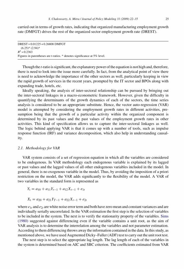
Approaching the issue in the light of Kaldor’s (1967) hypothesis we first take total organizedsector employment net of manufacturing as a function of manufacturing employment. The under-lying assumption is that the main driver is the manufacturing sector, and hence other activitieswithin the organized sector are largely determined by industry. Unit root test has been carried outto examine the stationarity property. Dickey–Fuller (DF) and Augmented Dickey–Fuller (ADF)test shows that in the level form the aggregate organized sector employment (net of manufactur-ing) is not stationary. On the other hand, ADF test confirms that in the second difference formafter taking log transformation these two variables are stationary. Hence, the regression has been

S. Chakravarty, A. Mitra / Journal of Policy Modeling 31 (2009) 22–35 25

carried out in terms of growth rates, indicating that organized manufacturing employment growthrate (DMFGT) drives the rest of the organized sector employment growth rate (DREST).

DREST = 0.01225 + 0.26808 DMFGT(6.25)* (2.94)*

R2 = 0.2363Figures in parentheses are t-ratios. * denotes significance at 5% level.

Though the t-ratio is significant, the explanatory power of the equation is not high and, therefore,there is need to look into the issue more carefully. In fact, from the analytical point of view thereis need to acknowledge the importance of the other sectors as well, particularly keeping in viewthe rapid growth of services in the recent years, prompted by the IT sector and BPOs along withexpanding trade, hotels, etc.

Ideally speaking, the analysis of inter-sectoral relationship can be pursued by bringing outthe inter-sectoral linkages in a macro-econometric framework. However, given the difficulty inquantifying the determinants of the growth dynamics of each of the sectors, the time seriesanalysis is considered to be an appropriate substitute. Hence, the vector auto-regression (VAR)model is attempted by considering the employment growth rates in different activities, pre-sumption being that the growth of a particular activity within the organized component isdetermined by its past values and the past values of the employment growth rates in otheractivities. This kind of specification allows us to capture the inter-sectoral linkages as well.The logic behind applying VAR is that it comes up with a number of tools, such as impulseresponse function (IRF) and variance decomposition, which also help in understanding causal-ity.

2.1. Methodology for VAR

VAR system consists of a set of regression equation in which all the variables are consideredto be endogenous. In VAR methodology each endogenous variable is explained by its laggedor past values and the lagged values of all other endogenous variables included in the model. Ingeneral, there is no exogenous variable in the model. Thus, by avoiding the imposition of a priorirestriction on the model, the VAR adds significantly to the flexibility of the model. A VAR oftwo variables in the standard form is represented as

Yt = a10 + a11Yt−1 + a12Xt−1 + e1t

Xt = a20 + a21YT−1 + a22Xt−1 + e2t

where e1t and e2t are white noise error term and both have zero mean and constant variances and areindividually serially uncorrelated. In the VAR estimation the first step is the selection of variablesto be included in the system. The next is to verify the stationarity property of the variables. Sims(1980) suggested against differencing even if the variable contains a unit root, as the aim ofVAR analysis is to determine the interrelation among the variables and not parameter estimation.According to them differencing throws away the information contained in the data. In this study, asmentioned above, we have used Augmented Dicky–Fuller (ADF) test to carry out the unit root test.

The next step is to select the appropriate lag length. The lag length of each of the variables inthe system is determined based on AIC and SBC criterion. The coefficients estimated from VAR

26 S. Chakravarty, A. Mitra / Journal of Policy Modeling 31 (2009) 22–35

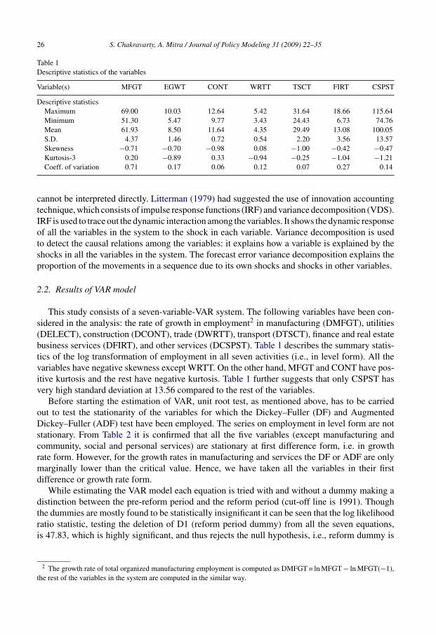
Table 1Descriptive statistics of the variables

Variable(s) MFGT EGWT CONT WRTT TSCT FIRT CSPST

Descriptive statisticsMaximum 69.00 10.03 12.64 5.42 31.64 18.66 115.64Minimum 51.30 5.47 9.77 3.43 24.43 6.73 74.76Mean 61.93 8.50 11.64 4.35 29.49 13.08 100.05S.D. 4.37 1.46 0.72 0.54 2.20 3.56 13.57Skewness −0.71 −0.70 −0.98 0.08 −1.00 −0.42 −0.47Kurtosis-3 0.20 −0.89 0.33 −0.94 −0.25 −1.04 −1.21Coeff. of variation 0.71 0.17 0.06 0.12 0.07 0.27 0.14

cannot be interpreted directly. Litterman (1979) had suggested the use of innovation accountingtechnique, which consists of impulse response functions (IRF) and variance decomposition (VDS).IRF is used to trace out the dynamic interaction among the variables. It shows the dynamic responseof all the variables in the system to the shock in each variable. Variance decomposition is usedto detect the causal relations among the variables: it explains how a variable is explained by theshocks in all the variables in the system. The forecast error variance decomposition explains theproportion of the movements in a sequence due to its own shocks and shocks in other variables.

2.2. Results of VAR model

This study consists of a seven-variable-VAR system. The following variables have been con-sidered in the analysis: the rate of growth in employment2 in manufacturing (DMFGT), utilities(DELECT), construction (DCONT), trade (DWRTT), transport (DTSCT), finance and real estatebusiness services (DFIRT), and other services (DCSPST). Table 1 describes the summary statis-tics of the log transformation of employment in all seven activities (i.e., in level form). All thevariables have negative skewness except WRTT. On the other hand, MFGT and CONT have pos-itive kurtosis and the rest have negative kurtosis. Table 1 further suggests that only CSPST hasvery high standard deviation at 13.56 compared to the rest of the variables.

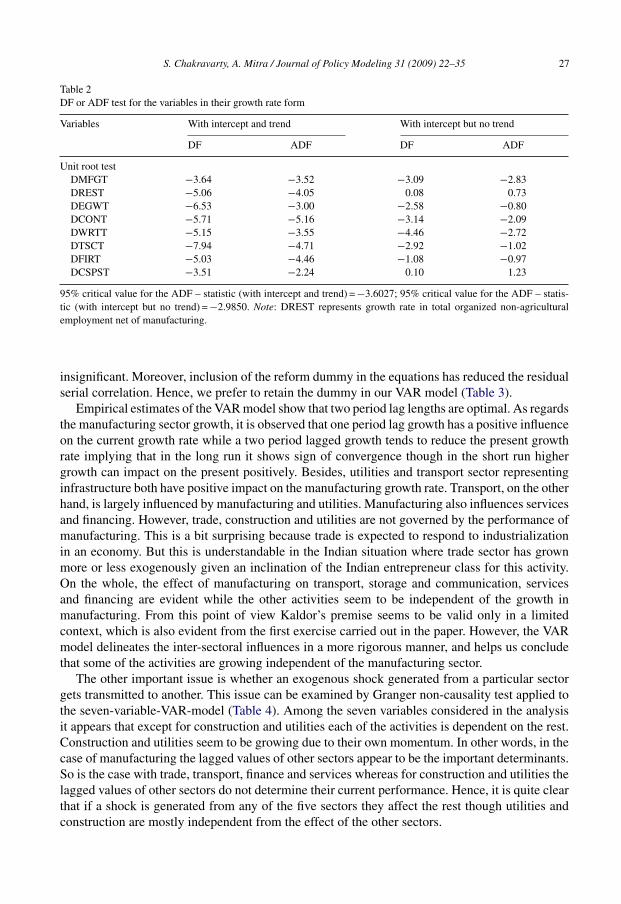
Before starting the estimation of VAR, unit root test, as mentioned above, has to be carriedout to test the stationarity of the variables for which the Dickey–Fuller (DF) and AugmentedDickey–Fuller (ADF) test have been employed. The series on employment in level form are notstationary. From Table 2 it is confirmed that all the five variables (except manufacturing andcommunity, social and personal services) are stationary at first difference form, i.e. in growthrate form. However, for the growth rates in manufacturing and services the DF or ADF are onlymarginally lower than the critical value. Hence, we have taken all the variables in their firstdifference or growth rate form.

While estimating the VAR model each equation is tried with and without a dummy making adistinction between the pre-reform period and the reform period (cut-off line is 1991). Thoughthe dummies are mostly found to be statistically insignificant it can be seen that the log likelihoodratio statistic, testing the deletion of D1 (reform period dummy) from all the seven equations,is 47.83, which is highly significant, and thus rejects the null hypothesis, i.e., reform dummy is

2 The growth rate of total organized manufacturing employment is computed as DMFGT = ln MFGT − ln MFGT(−1),the rest of the variables in the system are computed in the similar way.

S. Chakravarty, A. Mitra / Journal of Policy Modeling 31 (2009) 22–35 27

Table 2DF or ADF test for the variables in their growth rate form

Variables With intercept and trend With intercept but no trend

DF ADF DF ADF

Unit root testDMFGT −3.64 −3.52 −3.09 −2.83DREST −5.06 −4.05 0.08 0.73DEGWT −6.53 −3.00 −2.58 −0.80DCONT −5.71 −5.16 −3.14 −2.09DWRTT −5.15 −3.55 −4.46 −2.72DTSCT −7.94 −4.71 −2.92 −1.02DFIRT −5.03 −4.46 −1.08 −0.97DCSPST −3.51 −2.24 0.10 1.23

95% critical value for the ADF – statistic (with intercept and trend) = −3.6027; 95% critical value for the ADF – statis-tic (with intercept but no trend) = −2.9850. Note: DREST represents growth rate in total organized non-agriculturalemployment net of manufacturing.

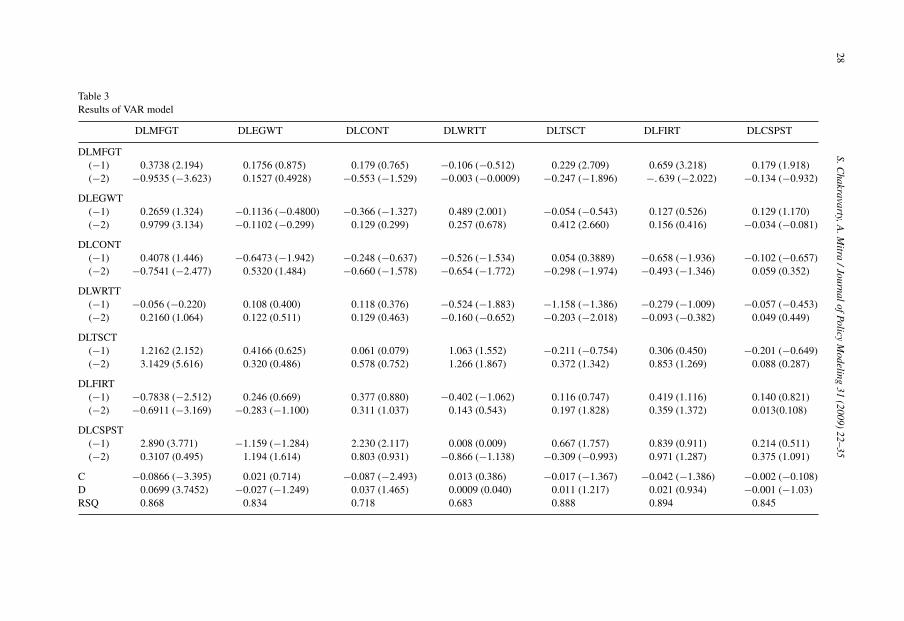
insignificant. Moreover, inclusion of the reform dummy in the equations has reduced the residualserial correlation. Hence, we prefer to retain the dummy in our VAR model (Table 3).

Empirical estimates of the VAR model show that two period lag lengths are optimal. As regardsthe manufacturing sector growth, it is observed that one period lag growth has a positive influenceon the current growth rate while a two period lagged growth tends to reduce the present growthrate implying that in the long run it shows sign of convergence though in the short run highergrowth can impact on the present positively. Besides, utilities and transport sector representinginfrastructure both have positive impact on the manufacturing growth rate. Transport, on the otherhand, is largely influenced by manufacturing and utilities. Manufacturing also influences servicesand financing. However, trade, construction and utilities are not governed by the performance ofmanufacturing. This is a bit surprising because trade is expected to respond to industrializationin an economy. But this is understandable in the Indian situation where trade sector has grownmore or less exogenously given an inclination of the Indian entrepreneur class for this activity.On the whole, the effect of manufacturing on transport, storage and communication, servicesand financing are evident while the other activities seem to be independent of the growth inmanufacturing. From this point of view Kaldor’s premise seems to be valid only in a limitedcontext, which is also evident from the first exercise carried out in the paper. However, the VARmodel delineates the inter-sectoral influences in a more rigorous manner, and helps us concludethat some of the activities are growing independent of the manufacturing sector.

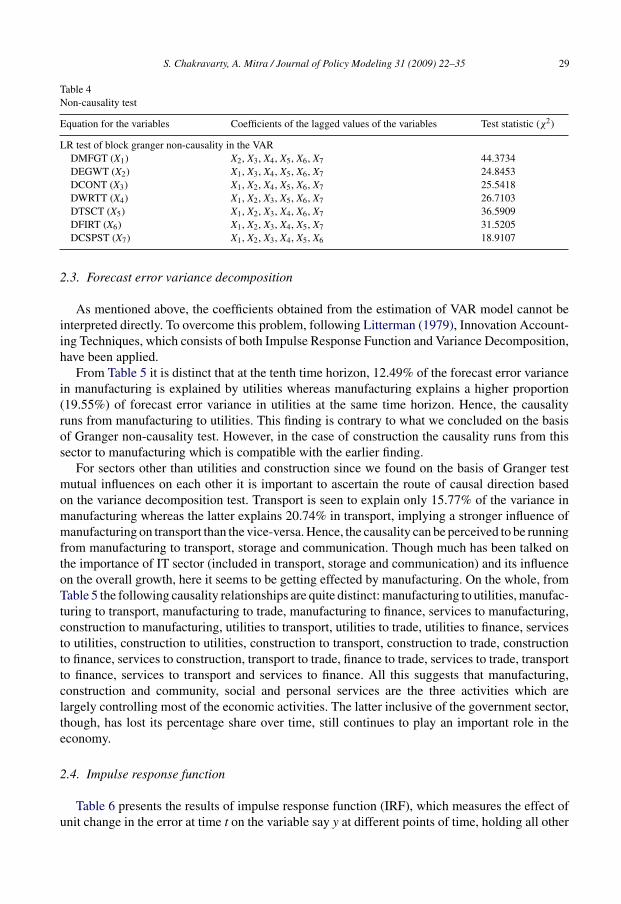
The other important issue is whether an exogenous shock generated from a particular sectorgets transmitted to another. This issue can be examined by Granger non-causality test applied tothe seven-variable-VAR-model (Table 4). Among the seven variables considered in the analysisit appears that except for construction and utilities each of the activities is dependent on the rest.Construction and utilities seem to be growing due to their own momentum. In other words, in thecase of manufacturing the lagged values of other sectors appear to be the important determinants.So is the case with trade, transport, finance and services whereas for construction and utilities thelagged values of other sectors do not determine their current performance. Hence, it is quite clearthat if a shock is generated from any of the five sectors they affect the rest though utilities andconstruction are mostly independent from the effect of the other sectors.

28S.C

hakravarty,A.M

itra/JournalofPolicy

Modeling

31(2009)

22–35

Table 3Results of VAR model

DLMFGT DLEGWT DLCONT DLWRTT DLTSCT DLFIRT DLCSPST

DLMFGT(−1) 0.3738 (2.194) 0.1756 (0.875) 0.179 (0.765) −0.106 (−0.512) 0.229 (2.709) 0.659 (3.218) 0.179 (1.918)(−2) −0.9535 (−3.623) 0.1527 (0.4928) −0.553 (−1.529) −0.003 (−0.0009) −0.247 (−1.896) −. 639 (−2.022) −0.134 (−0.932)

DLEGWT(−1) 0.2659 (1.324) −0.1136 (−0.4800) −0.366 (−1.327) 0.489 (2.001) −0.054 (−0.543) 0.127 (0.526) 0.129 (1.170)(−2) 0.9799 (3.134) −0.1102 (−0.299) 0.129 (0.299) 0.257 (0.678) 0.412 (2.660) 0.156 (0.416) −0.034 (−0.081)

DLCONT(−1) 0.4078 (1.446) −0.6473 (−1.942) −0.248 (−0.637) −0.526 (−1.534) 0.054 (0.3889) −0.658 (−1.936) −0.102 (−0.657)(−2) −0.7541 (−2.477) 0.5320 (1.484) −0.660 (−1.578) −0.654 (−1.772) −0.298 (−1.974) −0.493 (−1.346) 0.059 (0.352)

DLWRTT(−1) −0.056 (−0.220) 0.108 (0.400) 0.118 (0.376) −0.524 (−1.883) −1.158 (−1.386) −0.279 (−1.009) −0.057 (−0.453)(−2) 0.2160 (1.064) 0.122 (0.511) 0.129 (0.463) −0.160 (−0.652) −0.203 (−2.018) −0.093 (−0.382) 0.049 (0.449)

DLTSCT(−1) 1.2162 (2.152) 0.4166 (0.625) 0.061 (0.079) 1.063 (1.552) −0.211 (−0.754) 0.306 (0.450) −0.201 (−0.649)(−2) 3.1429 (5.616) 0.320 (0.486) 0.578 (0.752) 1.266 (1.867) 0.372 (1.342) 0.853 (1.269) 0.088 (0.287)

DLFIRT(−1) −0.7838 (−2.512) 0.246 (0.669) 0.377 (0.880) −0.402 (−1.062) 0.116 (0.747) 0.419 (1.116) 0.140 (0.821)(−2) −0.6911 (−3.169) −0.283 (−1.100) 0.311 (1.037) 0.143 (0.543) 0.197 (1.828) 0.359 (1.372) 0.013(0.108)

DLCSPST(−1) 2.890 (3.771) −1.159 (−1.284) 2.230 (2.117) 0.008 (0.009) 0.667 (1.757) 0.839 (0.911) 0.214 (0.511)(−2) 0.3107 (0.495) 1.194 (1.614) 0.803 (0.931) −0.866 (−1.138) −0.309 (−0.993) 0.971 (1.287) 0.375 (1.091)

C −0.0866 (−3.395) 0.021 (0.714) −0.087 (−2.493) 0.013 (0.386) −0.017 (−1.367) −0.042 (−1.386) −0.002 (−0.108)D 0.0699 (3.7452) −0.027 (−1.249) 0.037 (1.465) 0.0009 (0.040) 0.011 (1.217) 0.021 (0.934) −0.001 (−1.03)RSQ 0.868 0.834 0.718 0.683 0.888 0.894 0.845

S. Chakravarty, A. Mitra / Journal of Policy Modeling 31 (2009) 22–35 29

Table 4Non-causality test

Equation for the variables Coefficients of the lagged values of the variables Test statistic (χ2)

LR test of block granger non-causality in the VARDMFGT (X1) X2, X3, X4, X5, X6, X7 44.3734DEGWT (X2) X1, X3, X4, X5, X6, X7 24.8453DCONT (X3) X1, X2, X4, X5, X6, X7 25.5418DWRTT (X4) X1, X2, X3, X5, X6, X7 26.7103DTSCT (X5) X1, X2, X3, X4, X6, X7 36.5909DFIRT (X6) X1, X2, X3, X4, X5, X7 31.5205DCSPST (X7) X1, X2, X3, X4, X5, X6 18.9107

2.3. Forecast error variance decomposition

As mentioned above, the coefficients obtained from the estimation of VAR model cannot beinterpreted directly. To overcome this problem, following Litterman (1979), Innovation Account-ing Techniques, which consists of both Impulse Response Function and Variance Decomposition,have been applied.

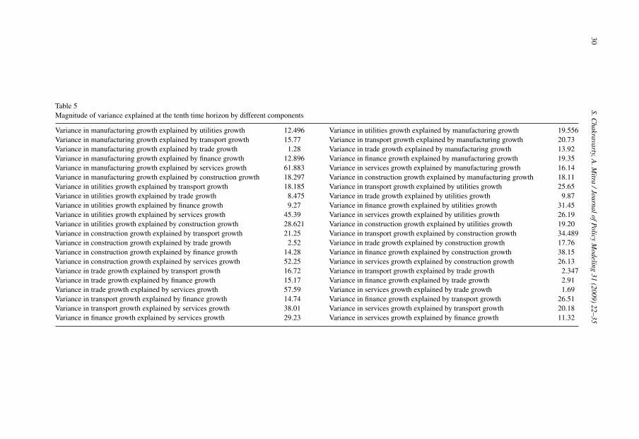
From Table 5 it is distinct that at the tenth time horizon, 12.49% of the forecast error variancein manufacturing is explained by utilities whereas manufacturing explains a higher proportion(19.55%) of forecast error variance in utilities at the same time horizon. Hence, the causalityruns from manufacturing to utilities. This finding is contrary to what we concluded on the basisof Granger non-causality test. However, in the case of construction the causality runs from thissector to manufacturing which is compatible with the earlier finding.

For sectors other than utilities and construction since we found on the basis of Granger testmutual influences on each other it is important to ascertain the route of causal direction basedon the variance decomposition test. Transport is seen to explain only 15.77% of the variance inmanufacturing whereas the latter explains 20.74% in transport, implying a stronger influence ofmanufacturing on transport than the vice-versa. Hence, the causality can be perceived to be runningfrom manufacturing to transport, storage and communication. Though much has been talked onthe importance of IT sector (included in transport, storage and communication) and its influenceon the overall growth, here it seems to be getting effected by manufacturing. On the whole, fromTable 5 the following causality relationships are quite distinct: manufacturing to utilities, manufac-turing to transport, manufacturing to trade, manufacturing to finance, services to manufacturing,construction to manufacturing, utilities to transport, utilities to trade, utilities to finance, servicesto utilities, construction to utilities, construction to transport, construction to trade, constructionto finance, services to construction, transport to trade, finance to trade, services to trade, transportto finance, services to transport and services to finance. All this suggests that manufacturing,construction and community, social and personal services are the three activities which arelargely controlling most of the economic activities. The latter inclusive of the government sector,though, has lost its percentage share over time, still continues to play an important role in theeconomy.

2.4. Impulse response function

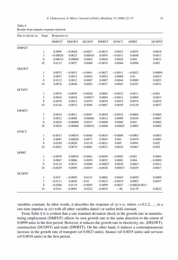
Table 6 presents the results of impulse response function (IRF), which measures the effect ofunit change in the error at time t on the variable say y at different points of time, holding all other

30S.C

hakravarty,A.M

itra/JournalofPolicy

Modeling

31(2009)

22–35

Table 5Magnitude of variance explained at the tenth time horizon by different components

Variance in manufacturing growth explained by utilities growth 12.496 Variance in utilities growth explained by manufacturing growth 19.556Variance in manufacturing growth explained by transport growth 15.77 Variance in transport growth explained by manufacturing growth 20.73Variance in manufacturing growth explained by trade growth 1.28 Variance in trade growth explained by manufacturing growth 13.92Variance in manufacturing growth explained by finance growth 12.896 Variance in finance growth explained by manufacturing growth 19.35Variance in manufacturing growth explained by services growth 61.883 Variance in services growth explained by manufacturing growth 16.14Variance in manufacturing growth explained by construction growth 18.297 Variance in construction growth explained by manufacturing growth 18.11Variance in utilities growth explained by transport growth 18.185 Variance in transport growth explained by utilities growth 25.65Variance in utilities growth explained by trade growth 8.475 Variance in trade growth explained by utilities growth 9.87Variance in utilities growth explained by finance growth 9.27 Variance in finance growth explained by utilities growth 31.45Variance in utilities growth explained by services growth 45.39 Variance in services growth explained by utilities growth 26.19Variance in utilities growth explained by construction growth 28.621 Variance in construction growth explained by utilities growth 19.20Variance in construction growth explained by transport growth 21.25 Variance in transport growth explained by construction growth 34.489Variance in construction growth explained by trade growth 2.52 Variance in trade growth explained by construction growth 17.76Variance in construction growth explained by finance growth 14.28 Variance in finance growth explained by construction growth 38.15Variance in construction growth explained by services growth 52.25 Variance in services growth explained by construction growth 26.13Variance in trade growth explained by transport growth 16.72 Variance in transport growth explained by trade growth 2.347Variance in trade growth explained by finance growth 15.17 Variance in finance growth explained by trade growth 2.91Variance in trade growth explained by services growth 57.59 Variance in services growth explained by trade growth 1.69Variance in transport growth explained by finance growth 14.74 Variance in finance growth explained by transport growth 26.51Variance in transport growth explained by services growth 38.01 Variance in services growth explained by transport growth 20.18Variance in finance growth explained by services growth 29.23 Variance in services growth explained by finance growth 11.32

S. Chakravarty, A. Mitra / Journal of Policy Modeling 31 (2009) 22–35 31

Table 6Results from impulse response function

Due to shocks in Steps Responses to

DMFGT DEGWT DCONT DWRTT DTSCT DFIRT DCSPST

DMFGT1 0.0099 −0.0028 −0.0027 −0.0015 0.0023 0.0035 0.00183 −0.00028 0.0023 0.00018 0.0095 −0.0013 0.0048 0.00118 0.00635 0.00009 0.0062 0.0044 0.0026 0.005 0.0011

10 0.0115 0.0027 0.0068 −0.0076 0.0044 0.0098 0.003

DEGWT1 0.0075 −0.0033 −0.0061 −0.0027 −0.0011 −0.0023 0.000913 0.0057 0.0015 0.0043 0.0052 0.0008 0.01 0.00198 0.0112 0.0012 0.0087 0.0007 0.0044 0.0089 0.0023

10 0.0076 0.0046 0.0063 −0.0037 0.0042 0.0101 0.0031

DCONT1 0.0076 −0.0054 −0.0026 0.0065 −0.0012 0.0011 −0.0013 0.0016 0.0034 0.00073 0.0084 −0.0011 0.0069 0.00138 0.0078 0.0012 0.0075 0.0039 0.0035 0.0074 0.0019

10 0.0144 0.0033 0.0096 −0.0087 0.0059 0.0129 0.0037

DWRTT1 0.0016 −0.0011 −0.0047 −0.0054 −0.0032 −0.0066 −0.00053 0.0012 −0.0006 0.00046 0.0012 0.0009 0.0036 0.00078 0.0028 −0.00008 0.0015 −0.0008 0.0009 0.001 0.0002

10 0.0034 −0.00008 0.00018 −0.0008 0.00025 0.0003 0.0002

DTSCT1 −0.0013 0.00076 −0.0064 −0.0019 −0.0009 −0.0003 0.00033 0.0083 0.00056 0.0077 0.0043 0.001 0.0079 0.00038 0.0169 −0.0028 0.0118 −0.0031 0.005 0.0091 0.002

10 −0.0022 0.0074 −0.0001 −0.0031 0.0018 0.0067 0.002

DFIRT1 −0.0059 0.00034 −0.0041 −0.0049 −0.0003 −0.001 0.00013 0.0067 0.0006 0.0059 0.0032 0.0003 0.004 −0.00098 0.0134 0.0033 0.0088 −0.00027 0.0036 0.0063 0.0012

10 −0.0039 0.0059 −0.0015 −0.0026 0.00073 0.0039 0.0017

DCSPST1 0.019 −0.0095 0.0131 0.0002 0.0045 0.0029 0.00093 −0.0111 0.0056 −0.01 −0.0015 −0.0019 0.0003 0.00378 −0.0206 0.0119 −0.0095 0.0099 −0.0027 −0.00020.0013

10 0.0341 −0.0091 0.0222 −0.0055 .−86 0.0139 0.0022

variables constant. In other words, it describes the response of y(t + s), where s = 0,1,2,. . ., to aone time impulse in y(t) with all other variables dated t or earlier held constant.

From Table 6 it is evident that a one standard deviation shock in the growth rate in manufac-turing employment (DMFGT) affects its own growth rate in the same direction to the extent of0.0099 units in the first period. However, it reduces the growth rate in electricity, etc. (DEGWT),construction (DCONT) and trade (DWRTT). On the other hand, it induces a contemporaneousincrease in the growth rate of transport (of 0.0023 units), finance (of 0.0035 units) and services(of 0.0018 units) in the first period.

32 S. Chakravarty, A. Mitra / Journal of Policy Modeling 31 (2009) 22–35

During the 3rd period, a one standard deviation shock in the growth rate in manufacturingreduces the manufacturing growth by 0.00028 units and increases the growth rate in all activitiesexcept transport. In the 10th period the growth rate in manufacturing increases by 0.0115 units, andgrowth rates in all other activities except trade also respond positively to one standard deviationshock in the growth rate of manufacturing. Thus we can conclude that both in the medium run(3rd period) and in the long run (10th period) the relationship between DMFGT and the rest ofthe variables remain consistent only with a few exceptions.

A one standard deviation shock in the growth rate in electricity affects its growth rate in theopposite direction to the extent of −0.0033 units in the 1st period. All other activities exceptmanufacturing also show a decline in their growth rates. In the 3rd period one standard deviationshock in the growth rate in electricity raises the growth rates in all activities. In the 8th period alsothe results remain almost the same and in the 10th period only trade is affected in the oppositedirection.

In the 1st period one standard deviation shock in construction (DCONT) reduces its owngrowth rate by −0.0026 units and affects the growth rates in electricity, transport and servicesnegatively too. For longer horizon, say at 10th period, one standard deviation shock in DCONTshows increase in all the variables except DWRTT.

One standard deviation shock in DWRTT in the first period changes all the variables in theopposite direction except manufacturing growth. However, at the 10th horizon except the growthin electricity and the growth in trade itself one standard deviation shock in the growth rate in tradeproduces positive responses in the growth in all other activities.

One standard deviation shock in DTSCT affects growth rates in all activities negatively exceptelectricity and services, at the first time horizon. However, growth rates in all activities respondpositively in the third time horizon. In the long run (10th time horizon) growth rates of manufac-turing, construction and trade decline and the rest improve in response to one standard deviationshock in the growth rate in transport.

Similarly one standard deviation shock in DFIRT in the short run (1st period) reduces thegrowth rate in all activities except electricity and services. But in the long run growth in transportand finance itself in addition to electricity and services also respond positively to one standarddeviation shock in the growth rate in finance.

One standard deviation shock in DCSPST in the short run raises the growth rate in all activitiesexcept electricity. On the other hand, at the third time horizon the growth rates of all activitiesexcept electricity, finance and services decline in response to one standard deviation shock inservices growth rate. In the long run, manufacturing, construction, finance and services move inthe positive direction and the rest in the negative direction in response to one standard deviationshock in the growth rate in services. All this tends to suggest that the inter-connections amongvarious activities cannot be ignored. Though manufacturing tends to provide a boost to most ofthe sectors in the medium and the long run, for the forecasting of the manufacturing activity theeffect of other activities on manufacturing cannot be ignored.

3. Predicting informal sector employment

One may argue that organized sector employment accounts for only around 10% of the totalemployment. Hence, the inter-sectoral relationships studied on the basis of VAR model maynot reflect much on the reality. However, the position that we take here is that based on thecross-sectional elasticity of unorganized or informal sector employment with respect to differentcomponents of the organized sector employment the former can be predicted for given levels of

S. Chakravarty, A. Mitra / Journal of Policy Modeling 31 (2009) 22–35 33

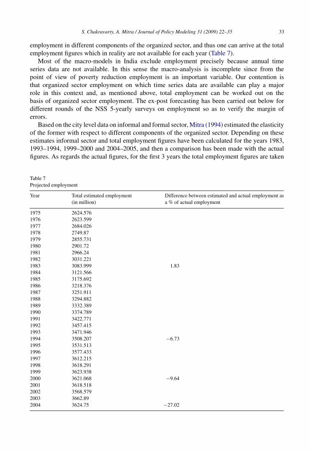
employment in different components of the organized sector, and thus one can arrive at the totalemployment figures which in reality are not available for each year (Table 7).

Most of the macro-models in India exclude employment precisely because annual timeseries data are not available. In this sense the macro-analysis is incomplete since from thepoint of view of poverty reduction employment is an important variable. Our contention isthat organized sector employment on which time series data are available can play a majorrole in this context and, as mentioned above, total employment can be worked out on thebasis of organized sector employment. The ex-post forecasting has been carried out below fordifferent rounds of the NSS 5-yearly surveys on employment so as to verify the margin oferrors.

Based on the city level data on informal and formal sector, Mitra (1994) estimated the elasticityof the former with respect to different components of the organized sector. Depending on theseestimates informal sector and total employment figures have been calculated for the years 1983,1993–1994, 1999–2000 and 2004–2005, and then a comparison has been made with the actualfigures. As regards the actual figures, for the first 3 years the total employment figures are taken

Table 7Projected employment

Year Total estimated employment(in million)

Difference between estimated and actual employment asa % of actual employment

1975 2624.5761976 2623.5991977 2684.0261978 2749.871979 2855.7311980 2901.721981 2966.241982 3031.2211983 3083.999 1.831984 3121.5661985 3175.6921986 3218.3761987 3251.9111988 3294.8821989 3332.3891990 3374.7891991 3422.7711992 3457.4151993 3471.9461994 3508.207 −6.731995 3531.5131996 3577.4331997 3612.2151998 3618.2911999 3623.9382000 3621.068 −9.642001 3618.5182002 3568.5792003 3662.892004 3624.75 −27.02

34 S. Chakravarty, A. Mitra / Journal of Policy Modeling 31 (2009) 22–35

from Economic Survey. For the year 2004–2005 the employment figures have been calculated inthe following manner.

The error of margin turns out to be only 2% for the year 1983, and then it goes up to 6.5 and9% subsequently. It is only in 2004–2005 the estimated employment falls short of the observedemployment to the extent of 21%. This could be partly due to the fact that absolute employ-ment figures for 2004–2005 have turned out to be slightly on the high side because of theassumption that population growth after 2001 has been same as that between 1991 and 2001.Also, it may be noted that work participation rates, which are expected to be more or less sta-ble over time, recorded a sharp increase in 2004–2005 relative to the earlier years. Hence, theincrease in the margin of error for the recent years is understandable. In such situations the cross-sectional elasticity of the informal sector employment with respect to different components offormal sector employment needs to be recalculated from the data for some of the more recentyears.

However, the point which still remains valid is that in the absence of time series informationon total employment, time series data on organized sector employment can be used to predictthe informal sector employment, using the cross-sectional elasticities and thus the total employ-ment can be derived without much flaw. These figures can then be used in the macro-model foremployment planning and poverty reduction strategies to be worked out.

4. Conclusion

This paper examines in the Indian context the role of manufacturing as the engine of growth.In spite of the differences in results following from different exercises certain important patternsare quite evident. While manufacturing appears to be one of the determinants of overall growth,various other activities also tend to show the impact on the rest. Inter-connections among variousactivities are also evident. Though manufacturing tends to provide a boost to most of the sectorsin the medium and the long run, for the forecasting of the manufacturing activity the effects ofother activities on manufacturing also need to be considered.

On the whole, manufacturing, construction and services emerge as the three important drivers ofgrowth. This may come as a bit of surprise because services inclusive of public administration areusually treated to be unproductive in nature. On the other hand, the IT sector included in transport,storage and communication does not emerge as a significant determinant of employment growththough much has been talked about this sector in the recent context of globalization and IT sectorrevolution.

One important policy prescription that follows directly from the analysis is to strengthenthe organized manufacturing sector as a large absorber of labour. Ironically the employmentshare of manufacturing in the Indian context has been pitiably low for almost the entire post-independence period of development. Total factor productivity growth based on labour intensivetechnology (or labour intensive technological progress) is an important consideration for therevival of the industrial sector. Besides, within the manufacturing sector components, which arerelatively labour intensive in nature, need to be identified and prioritized. The growth strategy andincentive structure have to be built with a focus on these components from the point of view ofemployment planning.

The policy makers have to look into the importance of other sectors as well. Construction, whichprovides work opportunities at decent wages to the unskilled and semi-skilled workers, must beconsidered as a part of employment strategy. Irrigation projects and building of infrastructure inthe rural and small urban areas would not only provide employment opportunities in the short

S. Chakravarty, A. Mitra / Journal of Policy Modeling 31 (2009) 22–35 35

run but also raise the income earning capacity of the households and their ability to contribute toeconomic growth in the long run.

Though downsizing of the public sector has been followed as a part of the labour market reformit has not been substituted by creation of adequate productive jobs elsewhere in the economy,particularly for those who are located at the bottom. On the other hand, contractualization hasreduced the due share of labour even in the organized sector, not to talk about the unorganized orinformal economy. The policy makers need to look into these issues carefully from the point ofview of human right and social justice.

Since the informal sector, as seen in our analysis, is dependent on the performance of theorganized or formal sector, by strengthening the inter-sectoral linkages organized industry cangenerate demand for several complementary and ancillary components manufactured within theinformal sector. This in turn would result in enhanced labour demand and improved earningsin the informal sector. Skill formation and credit assistance are the two other ways of raisingproductivity in the informal sector for which the State has to take initiative in a significant way.

References

Bhattacharya, B. B., & Mitra, A. (1989), Agriculture-Industry Growth Rates: Widening Disparity: An Explanation,Economic and Political Weekly, August 26.

Bhattacharya, B. B., & Mitra, A. (1990), Excess Growth of the Tertiary Sector: Issues and Implications, Economic andPolitical Weekly, November 3.

Bussolo, M. A., Mizzala, & Romaguera, P. (2002). Beyond Heckscher-Ohlin: Trade and labour market interactions in acase study for Chile. Journal of Policy Modeling, 24(7–8), 636–639.

Dasgupta, S. and Singh, A. (2006) “Will Services be the New Engine of Economic Growth in India ?” ESRC Centre forBusiness Research – Working Papers wp310, ESRC Centre for Business Research.

Dawson, P. J. (2006). The export–income relationship and trade liberalisation in Bangladesh. Journal of Policy Modeling,28(8), 889–896.

Hasan, R. (2003). The impact of trade and labour market regulations on employment and wages: Evidence from developingcountries. In R. Hasan & D. Mitra (Eds.), The Impact of Trade on Labour: Issues, Perspectives and Experiences fromDeveloping Asia. Amsterdam: North Holland, Elsevier.

Kaldor, N. (1967). Strategic factors in economic development. Ithaca: Cornell University Press.Kwack, S. Y., & Sun, L. Y. (2005). Economies of scale, technological progress, and the sources of economic growth: Case

of Korea, 1969–2000. Journal of Policy Modeling, 27(3), 265–283.Litterman, R. (1979). Techniques of forecasting using Vector Auto Regression, Working Paper No. 115, Federal Reserve

Bank of Minneapolis.McKinnon, R., & Schnabl, G. (2006). Devaluing the dollar: A critical analysis of William Cline’s case for a New Plaza

agreement. Journal of Policy Modeling, 28.Milas, C. (1999). Labour market decisions and Greek manufacturing competitiveness. Journal of Policy Modeling, 21(4),

505–513.Mitra, A. (1994). Urbanisation, Slums, Informal Sector Employment and Poverty: An Exploratory Study. New Delhi: D.

K. Publishers Distributors Pvt. Ltd.Panchmukhi, V. R., Nambiar, R. G., & Meheta, R. (1986), Structural change and economic growth in developing countries,

VIII World Economic Congress of the International Economic Association, Theme 4, December.Papola, T. S. (1981). Urban informal sector in a developing economy. Delhi: Vikas Publishing House.Rodrik, D. (1997). Has globalization gone too far? Washington, DC: Institute for International Economics.Romer, P. M. (1990). Endogenous technological change. Journal of Political Economy, 98(3).Sabolo, Y. (1975). Indian service industries. Geneva: ILO.Sims, C. A. (1980). Macroeconomics and Reality Econometrica, 48, 1–48.Stiglitz, J. E. (2003). Globalization and growth in emerging markets and the new economy. Journal of Policy Modeling,

25, 505–524.World Bank. (2004). Sustaining India’s services revolution: Access to foreign markets, domestic reform and international

negotiations. India: South Asia Region.