Iterative methods for sparse linear systems (PDF)saad/PS/iter1.pdf · Iterative Methods for Sparse Linear Systems ... Iterative methods for solving general, ... ments revolutionized

Iterative Methodsfor Sparse

Linear Systems

Yousef Saad

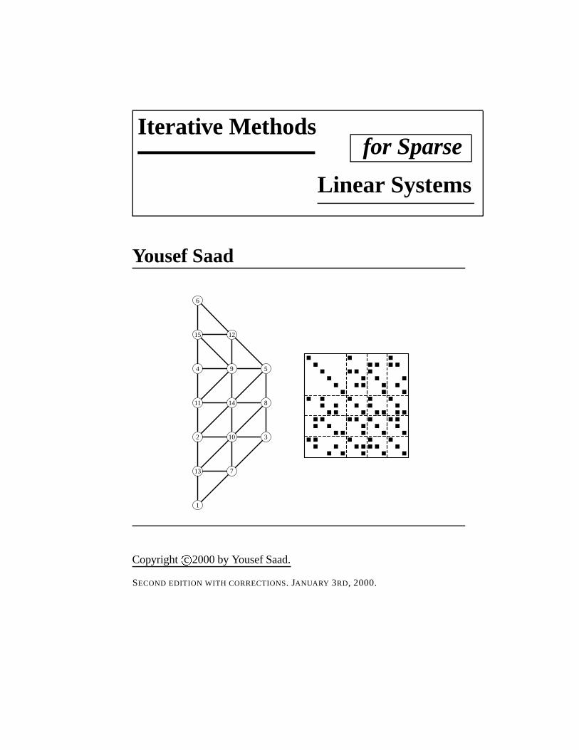
1

2 3

4 5

6

7

8

9

10

11

12

13

14

15

Copyright c�

2000 by Yousef Saad.

SECOND EDITION WITH CORRECTIONS. JANUARY 3RD, 2000.

��

PREFACE xiii

Acknowledgments . . . . . . . . . . . . . . . . . . . . . . . . . . . . . xivSuggestions for Teaching . . . . . . . . . . . . . . . . . . . . . . . . . xv

1 BACKGROUND IN LINEAR ALGEBRA 1

1.1 Matrices . . . . . . . . . . . . . . . . . . . . . . . . . . . . . . . . . . 11.2 Square Matrices and Eigenvalues . . . . . . . . . . . . . . . . . . . . . 31.3 Types of Matrices . . . . . . . . . . . . . . . . . . . . . . . . . . . . . 41.4 Vector Inner Products and Norms . . . . . . . . . . . . . . . . . . . . . 61.5 Matrix Norms . . . . . . . . . . . . . . . . . . . . . . . . . . . . . . . 81.6 Subspaces, Range, and Kernel . . . . . . . . . . . . . . . . . . . . . . . 91.7 Orthogonal Vectors and Subspaces . . . . . . . . . . . . . . . . . . . . 101.8 Canonical Forms of Matrices . . . . . . . . . . . . . . . . . . . . . . . 15

1.8.1 Reduction to the Diagonal Form . . . . . . . . . . . . . . . . . 151.8.2 The Jordan Canonical Form . . . . . . . . . . . . . . . . . . . . 161.8.3 The Schur Canonical Form . . . . . . . . . . . . . . . . . . . . 171.8.4 Application to Powers of Matrices . . . . . . . . . . . . . . . . 19

1.9 Normal and Hermitian Matrices . . . . . . . . . . . . . . . . . . . . . . 211.9.1 Normal Matrices . . . . . . . . . . . . . . . . . . . . . . . . . 211.9.2 Hermitian Matrices . . . . . . . . . . . . . . . . . . . . . . . . 24

1.10 Nonnegative Matrices, M-Matrices . . . . . . . . . . . . . . . . . . . . 261.11 Positive-Definite Matrices . . . . . . . . . . . . . . . . . . . . . . . . . 301.12 Projection Operators . . . . . . . . . . . . . . . . . . . . . . . . . . . . 33

1.12.1 Range and Null Space of a Projector . . . . . . . . . . . . . . . 331.12.2 Matrix Representations . . . . . . . . . . . . . . . . . . . . . . 351.12.3 Orthogonal and Oblique Projectors . . . . . . . . . . . . . . . . 351.12.4 Properties of Orthogonal Projectors . . . . . . . . . . . . . . . . 37

1.13 Basic Concepts in Linear Systems . . . . . . . . . . . . . . . . . . . . . 381.13.1 Existence of a Solution . . . . . . . . . . . . . . . . . . . . . . 381.13.2 Perturbation Analysis . . . . . . . . . . . . . . . . . . . . . . . 39

Exercises and Notes . . . . . . . . . . . . . . . . . . . . . . . . . . . . . . . 41

2 DISCRETIZATION OF PDES 44

2.1 Partial Differential Equations . . . . . . . . . . . . . . . . . . . . . . . 442.1.1 Elliptic Operators . . . . . . . . . . . . . . . . . . . . . . . . . 452.1.2 The Convection Diffusion Equation . . . . . . . . . . . . . . . 47

�

��

2.2 Finite Difference Methods . . . . . . . . . . . . . . . . . . . . . . . . . 472.2.1 Basic Approximations . . . . . . . . . . . . . . . . . . . . . . . 482.2.2 Difference Schemes for the Laplacean Operator . . . . . . . . . 492.2.3 Finite Differences for 1-D Problems . . . . . . . . . . . . . . . 512.2.4 Upwind Schemes . . . . . . . . . . . . . . . . . . . . . . . . . 512.2.5 Finite Differences for 2-D Problems . . . . . . . . . . . . . . . 54

2.3 The Finite Element Method . . . . . . . . . . . . . . . . . . . . . . . . 552.4 Mesh Generation and Refinement . . . . . . . . . . . . . . . . . . . . . 612.5 Finite Volume Method . . . . . . . . . . . . . . . . . . . . . . . . . . . 63Exercises and Notes . . . . . . . . . . . . . . . . . . . . . . . . . . . . . . . 66

3 SPARSE MATRICES 68

3.1 Introduction . . . . . . . . . . . . . . . . . . . . . . . . . . . . . . . . 683.2 Graph Representations . . . . . . . . . . . . . . . . . . . . . . . . . . . 70

3.2.1 Graphs and Adjacency Graphs . . . . . . . . . . . . . . . . . . 703.2.2 Graphs of PDE Matrices . . . . . . . . . . . . . . . . . . . . . 72

3.3 Permutations and Reorderings . . . . . . . . . . . . . . . . . . . . . . . 723.3.1 Basic Concepts . . . . . . . . . . . . . . . . . . . . . . . . . . 723.3.2 Relations with the Adjacency Graph . . . . . . . . . . . . . . . 753.3.3 Common Reorderings . . . . . . . . . . . . . . . . . . . . . . . 753.3.4 Irreducibility . . . . . . . . . . . . . . . . . . . . . . . . . . . 83

3.4 Storage Schemes . . . . . . . . . . . . . . . . . . . . . . . . . . . . . . 843.5 Basic Sparse Matrix Operations . . . . . . . . . . . . . . . . . . . . . . 873.6 Sparse Direct Solution Methods . . . . . . . . . . . . . . . . . . . . . . 883.7 Test Problems . . . . . . . . . . . . . . . . . . . . . . . . . . . . . . . 88Exercises and Notes . . . . . . . . . . . . . . . . . . . . . . . . . . . . . . . 91

4 BASIC ITERATIVE METHODS 95

4.1 Jacobi, Gauss-Seidel, and SOR . . . . . . . . . . . . . . . . . . . . . . 954.1.1 Block Relaxation Schemes . . . . . . . . . . . . . . . . . . . . 984.1.2 Iteration Matrices and Preconditioning . . . . . . . . . . . . . . 102

4.2 Convergence . . . . . . . . . . . . . . . . . . . . . . . . . . . . . . . . 1044.2.1 General Convergence Result . . . . . . . . . . . . . . . . . . . 1044.2.2 Regular Splittings . . . . . . . . . . . . . . . . . . . . . . . . . 1074.2.3 Diagonally Dominant Matrices . . . . . . . . . . . . . . . . . . 1084.2.4 Symmetric Positive Definite Matrices . . . . . . . . . . . . . . 1124.2.5 Property A and Consistent Orderings . . . . . . . . . . . . . . . 112

4.3 Alternating Direction Methods . . . . . . . . . . . . . . . . . . . . . . 116Exercises and Notes . . . . . . . . . . . . . . . . . . . . . . . . . . . . . . . 119

5 PROJECTION METHODS 122

5.1 Basic Definitions and Algorithms . . . . . . . . . . . . . . . . . . . . . 1225.1.1 General Projection Methods . . . . . . . . . . . . . . . . . . . 1235.1.2 Matrix Representation . . . . . . . . . . . . . . . . . . . . . . . 124

5.2 General Theory . . . . . . . . . . . . . . . . . . . . . . . . . . . . . . 1265.2.1 Two Optimality Results . . . . . . . . . . . . . . . . . . . . . . 126

� � ��

5.2.2 Interpretation in Terms of Projectors . . . . . . . . . . . . . . . 1275.2.3 General Error Bound . . . . . . . . . . . . . . . . . . . . . . . 129

5.3 One-Dimensional Projection Processes . . . . . . . . . . . . . . . . . . 1315.3.1 Steepest Descent . . . . . . . . . . . . . . . . . . . . . . . . . 1325.3.2 Minimal Residual (MR) Iteration . . . . . . . . . . . . . . . . . 1345.3.3 Residual Norm Steepest Descent . . . . . . . . . . . . . . . . . 136

5.4 Additive and Multiplicative Processes . . . . . . . . . . . . . . . . . . . 136Exercises and Notes . . . . . . . . . . . . . . . . . . . . . . . . . . . . . . . 139

6 KRYLOV SUBSPACE METHODS – PART I 144

6.1 Introduction . . . . . . . . . . . . . . . . . . . . . . . . . . . . . . . . 1446.2 Krylov Subspaces . . . . . . . . . . . . . . . . . . . . . . . . . . . . . 1456.3 Arnoldi’s Method . . . . . . . . . . . . . . . . . . . . . . . . . . . . . 147

6.3.1 The Basic Algorithm . . . . . . . . . . . . . . . . . . . . . . . 1476.3.2 Practical Implementations . . . . . . . . . . . . . . . . . . . . . 149

6.4 Arnoldi’s Method for Linear Systems (FOM) . . . . . . . . . . . . . . . 1526.4.1 Variation 1: Restarted FOM . . . . . . . . . . . . . . . . . . . . 1546.4.2 Variation 2: IOM and DIOM . . . . . . . . . . . . . . . . . . . 155

6.5 GMRES . . . . . . . . . . . . . . . . . . . . . . . . . . . . . . . . . . 1586.5.1 The Basic GMRES Algorithm . . . . . . . . . . . . . . . . . . 1586.5.2 The Householder Version . . . . . . . . . . . . . . . . . . . . . 1596.5.3 Practical Implementation Issues . . . . . . . . . . . . . . . . . 1616.5.4 Breakdown of GMRES . . . . . . . . . . . . . . . . . . . . . . 1656.5.5 Relations between FOM and GMRES . . . . . . . . . . . . . . 1656.5.6 Variation 1: Restarting . . . . . . . . . . . . . . . . . . . . . . 1686.5.7 Variation 2: Truncated GMRES Versions . . . . . . . . . . . . . 169

6.6 The Symmetric Lanczos Algorithm . . . . . . . . . . . . . . . . . . . . 1746.6.1 The Algorithm . . . . . . . . . . . . . . . . . . . . . . . . . . . 1746.6.2 Relation with Orthogonal Polynomials . . . . . . . . . . . . . . 175

6.7 The Conjugate Gradient Algorithm . . . . . . . . . . . . . . . . . . . . 1766.7.1 Derivation and Theory . . . . . . . . . . . . . . . . . . . . . . 1766.7.2 Alternative Formulations . . . . . . . . . . . . . . . . . . . . . 1806.7.3 Eigenvalue Estimates from the CG Coefficients . . . . . . . . . 181

6.8 The Conjugate Residual Method . . . . . . . . . . . . . . . . . . . . . 1836.9 GCR, ORTHOMIN, and ORTHODIR . . . . . . . . . . . . . . . . . . . 1836.10 The Faber-Manteuffel Theorem . . . . . . . . . . . . . . . . . . . . . . 1866.11 Convergence Analysis . . . . . . . . . . . . . . . . . . . . . . . . . . . 188

6.11.1 Real Chebyshev Polynomials . . . . . . . . . . . . . . . . . . . 1886.11.2 Complex Chebyshev Polynomials . . . . . . . . . . . . . . . . 1896.11.3 Convergence of the CG Algorithm . . . . . . . . . . . . . . . . 1936.11.4 Convergence of GMRES . . . . . . . . . . . . . . . . . . . . . 194

6.12 Block Krylov Methods . . . . . . . . . . . . . . . . . . . . . . . . . . 197Exercises and Notes . . . . . . . . . . . . . . . . . . . . . . . . . . . . . . . 202

7 KRYLOV SUBSPACE METHODS – PART II 205

7.1 Lanczos Biorthogonalization . . . . . . . . . . . . . . . . . . . . . . . 205

��

7.1.1 The Algorithm . . . . . . . . . . . . . . . . . . . . . . . . . . . 2057.1.2 Practical Implementations . . . . . . . . . . . . . . . . . . . . . 208

7.2 The Lanczos Algorithm for Linear Systems . . . . . . . . . . . . . . . . 2107.3 The BCG and QMR Algorithms . . . . . . . . . . . . . . . . . . . . . . 210

7.3.1 The Biconjugate Gradient Algorithm . . . . . . . . . . . . . . . 2117.3.2 Quasi-Minimal Residual Algorithm . . . . . . . . . . . . . . . 212

7.4 Transpose-Free Variants . . . . . . . . . . . . . . . . . . . . . . . . . . 2147.4.1 Conjugate Gradient Squared . . . . . . . . . . . . . . . . . . . 2157.4.2 BICGSTAB . . . . . . . . . . . . . . . . . . . . . . . . . . . . 2177.4.3 Transpose-Free QMR (TFQMR) . . . . . . . . . . . . . . . . . 221


8 METHODS RELATED TO THE NORMAL EQUATIONS 230

8.1 The Normal Equations . . . . . . . . . . . . . . . . . . . . . . . . . . . 2308.2 Row Projection Methods . . . . . . . . . . . . . . . . . . . . . . . . . 232

8.2.1 Gauss-Seidel on the Normal Equations . . . . . . . . . . . . . . 2328.2.2 Cimmino’s Method . . . . . . . . . . . . . . . . . . . . . . . . 234

8.3 Conjugate Gradient and Normal Equations . . . . . . . . . . . . . . . . 2378.3.1 CGNR . . . . . . . . . . . . . . . . . . . . . . . . . . . . . . . 2378.3.2 CGNE . . . . . . . . . . . . . . . . . . . . . . . . . . . . . . . 238

8.4 Saddle-Point Problems . . . . . . . . . . . . . . . . . . . . . . . . . . . 240Exercises and Notes . . . . . . . . . . . . . . . . . . . . . . . . . . . . . . . 243

9 PRECONDITIONED ITERATIONS 245

9.1 Introduction . . . . . . . . . . . . . . . . . . . . . . . . . . . . . . . . 2459.2 Preconditioned Conjugate Gradient . . . . . . . . . . . . . . . . . . . . 246

9.2.1 Preserving Symmetry . . . . . . . . . . . . . . . . . . . . . . . 2469.2.2 Efficient Implementations . . . . . . . . . . . . . . . . . . . . . 249

9.3 Preconditioned GMRES . . . . . . . . . . . . . . . . . . . . . . . . . . 2519.3.1 Left-Preconditioned GMRES . . . . . . . . . . . . . . . . . . . 2519.3.2 Right-Preconditioned GMRES . . . . . . . . . . . . . . . . . . 2539.3.3 Split Preconditioning . . . . . . . . . . . . . . . . . . . . . . . 2549.3.4 Comparison of Right and Left Preconditioning . . . . . . . . . . 255

9.4 Flexible Variants . . . . . . . . . . . . . . . . . . . . . . . . . . . . . . 2569.4.1 Flexible GMRES . . . . . . . . . . . . . . . . . . . . . . . . . 2569.4.2 DQGMRES . . . . . . . . . . . . . . . . . . . . . . . . . . . . 259

9.5 Preconditioned CG for the Normal Equations . . . . . . . . . . . . . . . 2609.6 The CGW Algorithm . . . . . . . . . . . . . . . . . . . . . . . . . . . 261Exercises and Notes . . . . . . . . . . . . . . . . . . . . . . . . . . . . . . . 263

10 PRECONDITIONING TECHNIQUES 265

10.1 Introduction . . . . . . . . . . . . . . . . . . . . . . . . . . . . . . . . 26510.2 Jacobi, SOR, and SSOR Preconditioners . . . . . . . . . . . . . . . . . 26610.3 ILU Factorization Preconditioners . . . . . . . . . . . . . . . . . . . . 269

10.3.1 Incomplete LU Factorizations . . . . . . . . . . . . . . . . . . . 27010.3.2 Zero Fill-in ILU (ILU(0)) . . . . . . . . . . . . . . . . . . . . . 275

� � ��

10.3.3 Level of Fill and ILU(� ) . . . . . . . . . . . . . . . . . . . . . . 27810.3.4 Matrices with Regular Structure . . . . . . . . . . . . . . . . . 28110.3.5 Modified ILU (MILU) . . . . . . . . . . . . . . . . . . . . . . 286

10.4 Threshold Strategies and ILUT . . . . . . . . . . . . . . . . . . . . . . 28710.4.1 The ILUT Approach . . . . . . . . . . . . . . . . . . . . . . . 28810.4.2 Analysis . . . . . . . . . . . . . . . . . . . . . . . . . . . . . . 28910.4.3 Implementation Details . . . . . . . . . . . . . . . . . . . . . . 29210.4.4 The ILUTP Approach . . . . . . . . . . . . . . . . . . . . . . . 29410.4.5 The ILUS Approach . . . . . . . . . . . . . . . . . . . . . . . . 296

10.5 Approximate Inverse Preconditioners . . . . . . . . . . . . . . . . . . . 29810.5.1 Approximating the Inverse of a Sparse Matrix . . . . . . . . . . 29910.5.2 Global Iteration . . . . . . . . . . . . . . . . . . . . . . . . . . 29910.5.3 Column-Oriented Algorithms . . . . . . . . . . . . . . . . . . . 30110.5.4 Theoretical Considerations . . . . . . . . . . . . . . . . . . . . 30310.5.5 Convergence of Self Preconditioned MR . . . . . . . . . . . . . 30510.5.6 Factored Approximate Inverses . . . . . . . . . . . . . . . . . . 30710.5.7 Improving a Preconditioner . . . . . . . . . . . . . . . . . . . . 310

10.6 Block Preconditioners . . . . . . . . . . . . . . . . . . . . . . . . . . . 31010.6.1 Block-Tridiagonal Matrices . . . . . . . . . . . . . . . . . . . . 31110.6.2 General Matrices . . . . . . . . . . . . . . . . . . . . . . . . . 312

10.7 Preconditioners for the Normal Equations . . . . . . . . . . . . . . . . 31310.7.1 Jacobi, SOR, and Variants . . . . . . . . . . . . . . . . . . . . . 31310.7.2 IC(0) for the Normal Equations . . . . . . . . . . . . . . . . . . 31410.7.3 Incomplete Gram-Schmidt and ILQ . . . . . . . . . . . . . . . 316


11 PARALLEL IMPLEMENTATIONS 324

11.1 Introduction . . . . . . . . . . . . . . . . . . . . . . . . . . . . . . . . 32411.2 Forms of Parallelism . . . . . . . . . . . . . . . . . . . . . . . . . . . . 325

11.2.1 Multiple Functional Units . . . . . . . . . . . . . . . . . . . . . 32511.2.2 Pipelining . . . . . . . . . . . . . . . . . . . . . . . . . . . . . 32611.2.3 Vector Processors . . . . . . . . . . . . . . . . . . . . . . . . . 32611.2.4 Multiprocessing and Distributed Computing . . . . . . . . . . . 326

11.3 Types of Parallel Architectures . . . . . . . . . . . . . . . . . . . . . . 32711.3.1 Shared Memory Computers . . . . . . . . . . . . . . . . . . . . 32711.3.2 Distributed Memory Architectures . . . . . . . . . . . . . . . . 329

11.4 Types of Operations . . . . . . . . . . . . . . . . . . . . . . . . . . . . 33111.4.1 Preconditioned CG . . . . . . . . . . . . . . . . . . . . . . . . 33211.4.2 GMRES . . . . . . . . . . . . . . . . . . . . . . . . . . . . . . 33211.4.3 Vector Operations . . . . . . . . . . . . . . . . . . . . . . . . . 33311.4.4 Reverse Communication . . . . . . . . . . . . . . . . . . . . . 334

11.5 Matrix-by-Vector Products . . . . . . . . . . . . . . . . . . . . . . . . 33511.5.1 The Case of Dense Matrices . . . . . . . . . . . . . . . . . . . 33511.5.2 The CSR and CSC Formats . . . . . . . . . . . . . . . . . . . . 33611.5.3 Matvecs in the Diagonal Format . . . . . . . . . . . . . . . . . 33911.5.4 The Ellpack-Itpack Format . . . . . . . . . . . . . . . . . . . . 340

� ��

11.5.5 The Jagged Diagonal Format . . . . . . . . . . . . . . . . . . . 34111.5.6 The Case of Distributed Sparse Matrices . . . . . . . . . . . . . 342

11.6 Standard Preconditioning Operations . . . . . . . . . . . . . . . . . . . 34511.6.1 Parallelism in Forward Sweeps . . . . . . . . . . . . . . . . . . 34611.6.2 Level Scheduling: the Case of 5-Point Matrices . . . . . . . . . 34611.6.3 Level Scheduling for Irregular Graphs . . . . . . . . . . . . . . 347


12 PARALLEL PRECONDITIONERS 353

12.1 Introduction . . . . . . . . . . . . . . . . . . . . . . . . . . . . . . . . 35312.2 Block-Jacobi Preconditioners . . . . . . . . . . . . . . . . . . . . . . . 35412.3 Polynomial Preconditioners . . . . . . . . . . . . . . . . . . . . . . . . 356

12.3.1 Neumann Polynomials . . . . . . . . . . . . . . . . . . . . . . 35612.3.2 Chebyshev Polynomials . . . . . . . . . . . . . . . . . . . . . . 35712.3.3 Least-Squares Polynomials . . . . . . . . . . . . . . . . . . . . 36012.3.4 The Nonsymmetric Case . . . . . . . . . . . . . . . . . . . . . 363

12.4 Multicoloring . . . . . . . . . . . . . . . . . . . . . . . . . . . . . . . 36512.4.1 Red-Black Ordering . . . . . . . . . . . . . . . . . . . . . . . . 36612.4.2 Solution of Red-Black Systems . . . . . . . . . . . . . . . . . . 36712.4.3 Multicoloring for General Sparse Matrices . . . . . . . . . . . . 368

12.5 Multi-Elimination ILU . . . . . . . . . . . . . . . . . . . . . . . . . . . 36912.5.1 Multi-Elimination . . . . . . . . . . . . . . . . . . . . . . . . . 37012.5.2 ILUM . . . . . . . . . . . . . . . . . . . . . . . . . . . . . . . 371

12.6 Distributed ILU and SSOR . . . . . . . . . . . . . . . . . . . . . . . . 37412.6.1 Distributed Sparse Matrices . . . . . . . . . . . . . . . . . . . . 374

12.7 Other Techniques . . . . . . . . . . . . . . . . . . . . . . . . . . . . . 37612.7.1 Approximate Inverses . . . . . . . . . . . . . . . . . . . . . . . 37712.7.2 Element-by-Element Techniques . . . . . . . . . . . . . . . . . 37712.7.3 Parallel Row Projection Preconditioners . . . . . . . . . . . . . 379


13 DOMAIN DECOMPOSITION METHODS 383

13.1 Introduction . . . . . . . . . . . . . . . . . . . . . . . . . . . . . . . . 38313.1.1 Notation . . . . . . . . . . . . . . . . . . . . . . . . . . . . . . 38413.1.2 Types of Partitionings . . . . . . . . . . . . . . . . . . . . . . . 38513.1.3 Types of Techniques . . . . . . . . . . . . . . . . . . . . . . . . 386

13.2 Direct Solution and the Schur Complement . . . . . . . . . . . . . . . . 38813.2.1 Block Gaussian Elimination . . . . . . . . . . . . . . . . . . . 38813.2.2 Properties of the Schur Complement . . . . . . . . . . . . . . . 38913.2.3 Schur Complement for Vertex-Based Partitionings . . . . . . . . 39013.2.4 Schur Complement for Finite-Element Partitionings . . . . . . . 393

13.3 Schwarz Alternating Procedures . . . . . . . . . . . . . . . . . . . . . . 39513.3.1 Multiplicative Schwarz Procedure . . . . . . . . . . . . . . . . 39513.3.2 Multiplicative Schwarz Preconditioning . . . . . . . . . . . . . 40013.3.3 Additive Schwarz Procedure . . . . . . . . . . . . . . . . . . . 40213.3.4 Convergence . . . . . . . . . . . . . . . . . . . . . . . . . . . . 404

� � ��

13.4 Schur Complement Approaches . . . . . . . . . . . . . . . . . . . . . . 40813.4.1 Induced Preconditioners . . . . . . . . . . . . . . . . . . . . . . 40813.4.2 Probing . . . . . . . . . . . . . . . . . . . . . . . . . . . . . . 41013.4.3 Preconditioning Vertex-Based Schur Complements . . . . . . . 411

13.5 Full Matrix Methods . . . . . . . . . . . . . . . . . . . . . . . . . . . . 41213.6 Graph Partitioning . . . . . . . . . . . . . . . . . . . . . . . . . . . . . 414

13.6.1 Basic Definitions . . . . . . . . . . . . . . . . . . . . . . . . . 41413.6.2 Geometric Approach . . . . . . . . . . . . . . . . . . . . . . . 41513.6.3 Spectral Techniques . . . . . . . . . . . . . . . . . . . . . . . . 41713.6.4 Graph Theory Techniques . . . . . . . . . . . . . . . . . . . . . 418


REFERENCES 425

INDEX 439

xii

��

Iterative methods for solving general, large sparse linear systems have been gainingpopularity in many areas of scientific computing. Until recently, direct solution methodswere often preferred to iterative methods in real applications because of their robustnessand predictable behavior. However, a number of efficient iterative solvers were discoveredand the increased need for solving very large linear systems triggered a noticeable andrapid shift toward iterative techniques in many applications.

This trend can be traced back to the 1960s and 1970s when two important develop-ments revolutionized solution methods for large linear systems. First was the realizationthat one can take advantage of “sparsity” to design special direct methods that can bequite economical. Initiated by electrical engineers, these “direct sparse solution methods”led to the development of reliable and efficient general-purpose direct solution softwarecodes over the next three decades. Second was the emergence of preconditioned conjugategradient-like methods for solving linear systems. It was found that the combination of pre-conditioning and Krylov subspace iterations could provide efficient and simple “general-purpose” procedures that could compete with direct solvers. Preconditioning involves ex-ploiting ideas from sparse direct solvers. Gradually, iterative methods started to approachthe quality of direct solvers. In earlier times, iterative methods were often special-purposein nature. They were developed with certain applications in mind, and their efficiency reliedon many problem-dependent parameters.

Now, three-dimensional models are commonplace and iterative methods are al-most mandatory. The memory and the computational requirements for solving three-dimensional Partial Differential Equations, or two-dimensional ones involving manydegrees of freedom per point, may seriously challenge the most efficient direct solversavailable today. Also, iterative methods are gaining ground because they are easier toimplement efficiently on high-performance computers than direct methods.

My intention in writing this volume is to provide up-to-date coverage of iterative meth-ods for solving large sparse linear systems. I focused the book on practical methods thatwork for general sparse matrices rather than for any specific class of problems. It is indeedbecoming important to embrace applications not necessarily governed by Partial Differ-ential Equations, as these applications are on the rise. Apart from two recent volumes byAxelsson [15] and Hackbusch [116], few books on iterative methods have appeared sincethe excellent ones by Varga [213]. and later Young [232]. Since then, researchers and prac-titioners have achieved remarkable progress in the development and use of effective iter-ative methods. Unfortunately, fewer elegant results have been discovered since the 1950sand 1960s. The field has moved in other directions. Methods have gained not only in effi-ciency but also in robustness and in generality. The traditional techniques which required

��

��

rather complicated procedures to determine optimal acceleration parameters have yieldedto the parameter-free conjugate gradient class of methods.

The primary aim of this book is to describe some of the best techniques available today,from both preconditioners and accelerators. One of the aims of the book is to provide agood mix of theory and practice. It also addresses some of the current research issuessuch as parallel implementations and robust preconditioners. The emphasis is on Krylovsubspace methods, currently the most practical and common group of techniques used inapplications. Although there is a tutorial chapter that covers the discretization of PartialDifferential Equations, the book is not biased toward any specific application area. Instead,the matrices are assumed to be general sparse, possibly irregularly structured.

The book has been structured in four distinct parts. The first part, Chapters 1 to 4,presents the basic tools. The second part, Chapters 5 to 8, presents projection methods andKrylov subspace techniques. The third part, Chapters 9 and 10, discusses precondition-ing. The fourth part, Chapters 11 to 13, discusses parallel implementations and parallelalgorithms.

��

I am grateful to a number of colleagues who proofread or reviewed different versions ofthe manuscript. Among them are Randy Bramley (University of Indiana at Bloomingtin),Xiao-Chuan Cai (University of Colorado at Boulder), Tony Chan (University of Californiaat Los Angeles), Jane Cullum (IBM, Yorktown Heights), Alan Edelman (MassachussettInstitute of Technology), Paul Fischer (Brown University), David Keyes (Old DominionUniversity), Beresford Parlett (University of California at Berkeley) and Shang-Hua Teng(University of Minnesota). Their numerous comments, corrections, and encouragementswere a highly appreciated contribution. In particular, they helped improve the presenta-tion considerably and prompted the addition of a number of topics missing from earlierversions.

This book evolved from several successive improvements of a set of lecture notes forthe course “Iterative Methods for Linear Systems” which I taught at the University of Min-nesota in the last few years. I apologize to those students who used the earlier error-ladenand incomplete manuscripts. Their input and criticism contributed significantly to improv-ing the manuscript. I also wish to thank those students at MIT (with Alan Edelman) andUCLA (with Tony Chan) who used this book in manuscript form and provided helpfulfeedback. My colleagues at the university of Minnesota, staff and faculty members, havehelped in different ways. I wish to thank in particular Ahmed Sameh for his encourage-ments and for fostering a productive environment in the department. Finally, I am gratefulto the National Science Foundation for their continued financial support of my research,part of which is represented in this work.

Yousef Saad

� ��

��

This book can be used as a text to teach a graduate-level course on iterative methods forlinear systems. Selecting topics to teach depends on whether the course is taught in amathematics department or a computer science (or engineering) department, and whetherthe course is over a semester or a quarter. Here are a few comments on the relevance of thetopics in each chapter.

For a graduate course in a mathematics department, much of the material in Chapter 1should be known already. For non-mathematics majors most of the chapter must be coveredor reviewed to acquire a good background for later chapters. The important topics forthe rest of the book are in Sections: 1.8.1, 1.8.3, 1.8.4, 1.9, 1.11. Section 1.12 is besttreated at the beginning of Chapter 5. Chapter 2 is essentially independent from the restand could be skipped altogether in a quarter course. One lecture on finite differences andthe resulting matrices would be enough for a non-math course. Chapter 3 should makethe student familiar with some implementation issues associated with iterative solutionprocedures for general sparse matrices. In a computer science or engineering department,this can be very relevant. For mathematicians, a mention of the graph theory aspects ofsparse matrices and a few storage schemes may be sufficient. Most students at this levelshould be familiar with a few of the elementary relaxation techniques covered in Chapter4. The convergence theory can be skipped for non-math majors. These methods are nowoften used as preconditioners and this may be the only motive for covering them.

Chapter 5 introduces key concepts and presents projection techniques in general terms.Non-mathematicians may wish to skip Section 5.2.3. Otherwise, it is recommended tostart the theory section by going back to Section 1.12 on general definitions on projectors.Chapters 6 and 7 represent the heart of the matter. It is recommended to describe the firstalgorithms carefully and put emphasis on the fact that they generalize the one-dimensionalmethods covered in Chapter 5. It is also important to stress the optimality properties ofthose methods in Chapter 6 and the fact that these follow immediately from the propertiesof projectors seen in Section 1.12. When covering the algorithms in Chapter 7, it is crucialto point out the main differences between them and those seen in Chapter 6. The variantssuch as CGS, BICGSTAB, and TFQMR can be covered in a short time, omitting details ofthe algebraic derivations or covering only one of the three. The class of methods based onthe normal equation approach, i.e., Chapter 8, can be skipped in a math-oriented course,especially in the case of a quarter system. For a semester course, selected topics may beSections 8.1, 8.2, and 8.4.

Currently, preconditioning is known to be the critical ingredient in the success of it-erative methods in solving real-life problems. Therefore, at least some parts of Chapter 9and Chapter 10 should be covered. Section 9.2 and (very briefly) 9.3 are recommended.From Chapter 10, discuss the basic ideas in Sections 10.1 through 10.3. The rest could beskipped in a quarter course.

Chapter 11 may be useful to present to computer science majors, but may be skimmedor skipped in a mathematics or an engineering course. Parts of Chapter 12 could be taughtprimarily to make the students aware of the importance of “alternative” preconditioners.Suggested selections are: 12.2, 12.4, and 12.7.2 (for engineers). Chapter 13 presents an im-

� � � ��

portant research area and is primilarily geared to mathematics majors. Computer scientistsor engineers may prefer to cover this material in less detail.

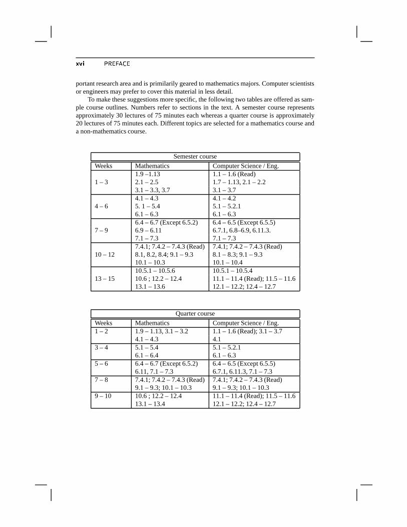
To make these suggestions more specific, the following two tables are offered as sam-ple course outlines. Numbers refer to sections in the text. A semester course representsapproximately 30 lectures of 75 minutes each whereas a quarter course is approximately20 lectures of 75 minutes each. Different topics are selected for a mathematics course anda non-mathematics course.

Semester course

Weeks Mathematics Computer Science / Eng.1.9 –1.13 1.1 – 1.6 (Read)

1 – 3 2.1 – 2.5 1.7 – 1.13, 2.1 – 2.23.1 – 3.3, 3.7 3.1 – 3.74.1 – 4.3 4.1 – 4.2

4 – 6 5. 1 – 5.4 5.1 – 5.2.16.1 – 6.3 6.1 – 6.36.4 – 6.7 (Except 6.5.2) 6.4 – 6.5 (Except 6.5.5)

7 – 9 6.9 – 6.11 6.7.1, 6.8–6.9, 6.11.3.7.1 – 7.3 7.1 – 7.37.4.1; 7.4.2 – 7.4.3 (Read) 7.4.1; 7.4.2 – 7.4.3 (Read)

10 – 12 8.1, 8.2, 8.4; 9.1 – 9.3 8.1 – 8.3; 9.1 – 9.310.1 – 10.3 10.1 – 10.410.5.1 – 10.5.6 10.5.1 – 10.5.4

13 – 15 10.6 ; 12.2 – 12.4 11.1 – 11.4 (Read); 11.5 – 11.613.1 – 13.6 12.1 – 12.2; 12.4 – 12.7

Quarter course

Weeks Mathematics Computer Science / Eng.1 – 2 1.9 – 1.13, 3.1 – 3.2 1.1 – 1.6 (Read); 3.1 – 3.7

4.1 – 4.3 4.13 – 4 5.1 – 5.4 5.1 – 5.2.1

6.1 – 6.4 6.1 – 6.35 – 6 6.4 – 6.7 (Except 6.5.2) 6.4 – 6.5 (Except 6.5.5)

6.11, 7.1 – 7.3 6.7.1, 6.11.3, 7.1 – 7.37 – 8 7.4.1; 7.4.2 – 7.4.3 (Read) 7.4.1; 7.4.2 – 7.4.3 (Read)

9.1 – 9.3; 10.1 – 10.3 9.1 – 9.3; 10.1 – 10.39 – 10 10.6 ; 12.2 – 12.4 11.1 – 11.4 (Read); 11.5 – 11.6

13.1 – 13.4 12.1 – 12.2; 12.4 – 12.7

� � � � � � �

�

� � ��

�� ! #"%$�&(')� *�$+�,�)-/.�*�$�&0*�� $213.�45"6��$7&8$�9 $6*��)-#":�6.;-��<$� #"=�>�0-?9 �0-�$+��&@�!9 'A$�B�&8�15�� ?��&8$DCE�%$64=C!9(�F-G9 �E"H$�&5��! #"%$�&I�<JLK "MBA$6')�0-E�N1�� "+�?�G&8$6*�� $61O.�4PB��E�2� �RQ5�#S"+&T� U?"+��$6.)&0VD�)-�WX�F-#"+&I.)WYC��<$+�,"6��$Z$�9 $�Q5$�-#"H��&0VX-E.�"%�#"2� .[-\CE�%$<W\"6�!&8.[CE';�E.[C#"N"+��$B�.!.[]AJ ��$:�+.;-#*�$�&I'�$�-��<$,�!-��!9 VE�2� �^.�4�� "H$�&8�E"_� *�$,Q5$6"+�E.)WA�`&8$<aYC��0&8$+�L�,'�.!.)W?9 $6*�$�9.�4L]�-E.#1L9 $<WA'A$,�0-bQ5�E"6��$�Q5�E"_� �<�!9[�)-��!9 VE�2� �L�!-�WZ�0-b9 �0-�$+��&c�!9 'A$�B�&8�[J �d&8��W[� "2� .;-��!9 9 V#eQ5�)-#V/.�4^"+��$>�+.[-��<$� #"H�> �&8$+�H$�-#"%$<W7�+ �$<�E� f;�<�!9 9 Vb4T.!&�"6��$+�%$>�)-��!9 VE�%$6�b��#*�$7B�$<$�-'A$<��&8$<W`"H.#1g��&8W>Q5�#"+&T� �<$6�h��&i� �2�0-E'j4k&8.[Ql"+��$�W[� �H��&8$6"2� m+�E"_� .;-^.�4 �Y��&0"2� �)9!n(� op$�&q$�-#"2� �!9[aYC��E"_� .;-E�^�!-�WMB��2� �,&q$�9 �#U��#"2� .;-#Sr"rV! A$�Q5$6"6�E.)WA�<J ��$+�%$:�+.[-��<$� #"H�L��&8$N-E.#1sBA$2S�+.;Qt�0-E'�9 $+�H�(�0Q` �.)&0"H�)-#"gBA$+�<�)CE�H$@.�4u"+��$g"+&8$�-�Wt"H.#1g��&8WN �&I.6vw$<�2"2� .[-#Sw"rV! �$5Q5$6"+�E.)WA�15�� ,��#*�$`QL.!&8$:&I.;B!CE�k"(�6.;-#*�$�&I'A$�-��<$: �&8.[ A$�&I"_� $+�x�)-�WP&8$<aYC��0&8$LW[� op$�&8$�-#"g�!-��)9 V#S�2� �h"H.!.[9 �<J ��$`Q5�#"%$�&T� �!9��+.�*�$�&q$+W>�0-L"+�� g��! #"%$�&;1^�F9 9)BA$t��$�9 #4kC!9A�0-5$+�="%�!B!9 � �6��0-E'�H.;Q5$`"+��$+.!&0V,4q.)&y"+��$`�)9 '�.!&T� "+�!QL�L�)-�WbW!$6fz-��0-E',"6��$N-E.�"%�#"2� .;->CE�%$<W>"+�!&I.;CE'[�E.;C#""+��$,B�.!.;]�J

� � ��

{}|E{

For the sake of generality, all vector spaces considered in this chapter are complex, unlessotherwise stated. A complex ~��D� matrix � is an ~��R� array of complex numbers

��F�;�D�@��[�� ~ �d�}��[��E� � �The set of all ~�� matrices is a complex vector space denoted by �`��z� . The mainoperations with matrices are the following:� Addition: � � �� , where � � � , and � are matrices of size ~��D� and

� �0� �� 0� �� 0� � �@��[�<�u�� ~ ��/�O�;�+�u��

� �� (n�K � �[K � � � �� Multiplication by a scalar: � �� , where

� �F� ��G� �0� � �(��[�<�u�� ~ ��/��;�+�z�� Multiplication by another matrix:

� � �� where ��j��z� � ��j�>�� j�� , and

� �0� � �� Sometimes, a notation with column vectors and row vectors is used. The column vector�� is the vector consisting of the � -th column of � ,

�� !""#� � ��%$ �

...� � �

&('') �

Similarly, the notation � � will denote the � -th row of the matrix �� `��*w� � � �+� � $[��+� � �,+ �

For example, the following could be written

� ��*w� � �6� -$ ��6� � + �or

� �!"""#� � �%$. ��

& ''') �

The transpose of a matrix � in � ��z� is a matrix � in �t�>�u� whose elements aredefined by � �F� � � �6� �2�� ;��E� � �@�X� �;��E� ~ . It is denoted by �0/ . It is often morerelevant to use the transpose conjugate matrix denoted by �21 and defined by

� 1 �43� / � � / �in which the bar denotes the (element-wise) complex conjugation.

Matrices are strongly related to linear mappings between vector spaces of finite di-mension. This is because they represent these mappings with respect to two given bases:one for the initial vector space and the other for the image vector space, or range of � .

�� dK � �� @n zK � ��

�� {}|��

A matrix is square if it has the same number of columns and rows, i.e., if � � ~ . Animportant square matrix is the identity matrix� �� 0�� where � �F� is the Kronecker symbol. The identity matrix satisfies the equality � � � � � � �for every matrix � of size ~ . The inverse of a matrix, when it exists, is a matrix � such that

�N� � �� The inverse of � is denoted by �� .

The determinant of a matrix may be defined in several ways. For simplicity, the fol-lowing recursive definition is used here. The determinant of a � � � matrix *w� + is definedas the scalar � . Then the determinant of an ~��D~ matrix is given by

�� * � + � �� *�!P� + �#" � � � � �$� � * � � � + �where � � � is an * ~ !�� + � * ~ !�� + matrix obtained by deleting the first row and the � -thcolumn of � . A matrix is said to be singular when

�� * � + �&% and nonsingular otherwise.We have the following simple properties:� ��'� * �� + � ��'� * �}� + .� ��'� * � / + � ��'� * � + .� ��'� * � � + � � � ��'� * � + .� ��'� *�3� + � �� * � + .� ��'� * � + �� .

From the above definition of determinants it can be shown by induction that the func-tion that maps a given complex value ( to the value �*) * ( + � �$� � * � ! ( � + is a polynomialof degree ~ ; see Exercise 8. This is known as the characteristic polynomial of the matrix� .

+ �-,/.�01.q�2.4350 �76T�A complex scalar ( is called an eigenvalue of the square matrix � if

a nonzero vector 8 of �t� exists such that �98 � (78 . The vector 8 is called an eigenvectorof � associated with ( . The set of all the eigenvalues of � is called the spectrum of � andis denoted by : * � + .

A scalar ( is an eigenvalue of � if and only if�� * � ! ( � +<; �*) * ( + �=% . That is true

if and only if (iff thereafter) ( is a root of the characteristic polynomial. In particular, thereare at most ~ distinct eigenvalues.

It is clear that a matrix is singular if and only if it admits zero as an eigenvalue. A wellknown result in linear algebra is stated in the following proposition.

�5�<3/�<32>?.8�1.4350 �76T�A matrix � is nonsingular if and only if it admits an inverse.

� �� (n�K � �[K � � � �� Thus, the determinant of a matrix determines whether or not the matrix admits an inverse.

The maximum modulus of the eigenvalues is called spectral radius and is denoted by�* � + �* � + �� )�� ( � �

The trace of a matrix is equal to the sum of all its diagonal elements

�� * � + � �� q� �It can be easily shown that the trace of � is also equal to the sum of the eigenvalues of �counted with their multiplicities as roots of the characteristic polynomial.

�5�<3/�<32>?.q�2.4350 �76 �If ( is an eigenvalue of � , then 3( is an eigenvalue of �01 . An

eigenvector � of �01 associated with the eigenvalue 3( is called a left eigenvector of � .

When a distinction is necessary, an eigenvector of � is often called a right eigenvector.Therefore, the eigenvalue ( as well as the right and left eigenvectors, 8 and � , satisfy therelations

� 8 � (78 � � 1 � � (�� 1 �or, equivalently,

8 1 � 1 � 3(78 1 � � 1 � � 3(��

{b|��

The choice of a method for solving linear systems will often depend on the structure ofthe matrix � . One of the most important properties of matrices is symmetry, because ofits impact on the eigenstructure of � . A number of other classes of matrices also haveparticular eigenstructures. The most important ones are listed below:

� Symmetric matrices: �0/ � � .� Hermitian matrices: �01 � � .� Skew-symmetric matrices: �0/ � ! � .� Skew-Hermitian matrices: �01 ��! � .� Normal matrices: �01�� :� 1 .� Nonnegative matrices: � �0�� %p�g�<�=�/��;��E� ~ (similar definition for nonpositive,positive, and negative matrices).� Unitary matrices: � 1��

.

�� dK � � �

It is worth noting that a unitary matrix � is a matrix whose inverse is its transpose conjugate�21 , since

� 1 � � � � � � � � � 1 � �� J ��A matrix � such that � 1�� is diagonal is often called orthogonal.

Some matrices have particular structures that are often convenient for computationalpurposes. The following list, though incomplete, gives an idea of these special matriceswhich play an important role in numerical analysis and scientific computing applications.

� Diagonal matrices: � �0� �&% for �� . Notation:

� � � � �� *k� � � �+�%$-$[��+� �[��+ �� Upper triangular matrices: � �F� � % for �� .� Lower triangular matrices: � �F� � % for ��l� .� Upper bidiagonal matrices: � �0� �=% for ��s� or ��s� � � .� Lower bidiagonal matrices: �z�0�:�=% for ��s� or ��s�/! � .� Tridiagonal matrices: �z�0��&% for any pair �<�=� such that� �2!�� 3� . Notation:

� � � �� *k�Y�� 6��8�6�6�� " � + �� Banded matrices: � �0� �&% only if �*! �� , where �� and �� are twononnegative integers. The number ��p� ��,� � is called the bandwidth of � .� Upper Hessenberg matrices: � �0� � % for any pair �<�=� such that �� . LowerHessenberg matrices can be defined similarly.� Outer product matrices: � � 8 ��1 , where both 8 and � are vectors.� Permutation matrices: the columns of � are a permutation of the columns of theidentity matrix.� Block diagonal matrices: generalizes the diagonal matrix by replacing each diago-nal entry by a matrix. Notation:

� � �� * � � � � � $ $ ��E� � �)� + �� Block tridiagonal matrices: generalizes the tridiagonal matrix by replacing eachnonzero entry by a square matrix. Notation:

� � ��4�� * � � � � � � � � �8� � � � � � " � + �The above properties emphasize structure, i.e., positions of the nonzero elements with

respect to the zeros. Also, they assume that there are many zero elements or that the matrixis of low rank. This is in contrast with the classifications listed earlier, such as symmetryor normality.

� �� (n�K � �[K � � � ��

{b|��

An inner product on a (complex) vector space � is any mapping � from � �� into � ,

� �� *�g�� + �� which satisfies the following conditions:

�� *�x�� + is linear with respect to � , i.e.,

� * ( � � � � ( $�� $;�� + � ( � � *� � �� + � ( $ � *�$[�� + �� $ �� ( � � ( $ � � �� *�x�� + is Hermitian, i.e.,

� *�c�� + � � *��g�� + ��x�� *�x�� + is positive definite, i.e.,

� *�g�� + � %p�� %z�Note that (2) implies that � *�x�� + is real and therefore, (3) adds the constraint that � *��g�� +must also be positive for any nonzero � . For any � and � ,

� *�g� % + � � *�g� %z� � + �&%p� � *�x�� + �=%z�Similarly, � *�%p�� + � % for any � . Hence, � * %z�� + � � *��g� % + �&% for any � and � . In particularthe condition (3) can be rewritten as

� *�x�� + � % and � *��g�� + �=% iff �R�=%z�as can be readily shown. A useful relation satisfied by any inner product is the so-calledCauchy-Schwartz inequality:

� � *�x�� + � $ �� *��g�� + � *�c�� + � �� J � �The proof of this inequality begins by expanding � *�2! ( �c��2! ( � + using the properties of� ,

� *� ! ( �c�� ! ( � + � � *�g�� + ! 3(�� *�g�� + ! (�� *�c�� + � � ( � $ � *�c�� + �If � � % then the inequality is trivially satisfied. Assume that � � % and take ( �� *�g�� + � � *��y�� + . Then � *� ! ( �y�� ! ( � + � % shows the above equality

% �� *�� ! ( �c��! ( � + � � *�x�� + !l�� *��g�� + � $� *��c�� + �

� � *�g�� + � $� *�c�� +� � *�x�� + !� � *�x�� + � $� *�c�� + �

which yields the result (1.2).In the particular case of the vector space � � � � , a “canonical” inner product is the

Euclidean inner product. The Euclidean inner product of two vectors �R��*�g� + � �� and

�� XK � � � �� n� � � � � �@n � � � � � ��/� *�� + � �� of �j� is defined by

*�x�� + � �� y� 3�;�2� �� J � �which is often rewritten in matrix notation as*��g�� + � � 1 �x� �� J � �It is easy to verify that this mapping does indeed satisfy the three conditions required forinner products, listed above. A fundamental property of the Euclidean inner product inmatrix computations is the simple relation* � �x�� + ��*�g� � 1 � + � ��x�� 5� � �� J � �The proof of this is straightforward. The adjoint of � with respect to an arbitrary innerproduct is a matrix � such that * � �g�� + � *�x� � � + for all pairs of vectors � and � . A matrixis self-adjoint, or Hermitian with respect to this inner product, if it is equal to its adjoint.

The following proposition is a consequence of the equality (1.5).

�5�<3/�<32>?.8�1.4350 �76 Unitary matrices preserve the Euclidean inner product, i.e.,* � �x� � � + ��*�g�� +for any unitary matrix � and any vectors � and � .

�� 6Indeed, * � �g� � � + � *��g� � 1�� + � *��g�� + .

A vector norm on a vector space � is a real-valued function � � � � � on � , whichsatisfies the following three conditions:

� � � � � %z� � � � � � and� � � �=% iff �D�=% .� � � � � � � � � � � � �� .�� x�� .

For the particular case when � � �t� , we can associate with the inner product (1.3)the Euclidean norm of a complex vector defined by� � � $:� *�x�� + �� $ �It follows from Proposition 1.3 that a unitary matrix preserves the Euclidean norm metric,i.e., � � � � $:� � � � $!� ��g�The linear transformation associated with a unitary matrix � is therefore an isometry.

The most commonly used vector norms in numerical linear algebra are special casesof the Holder norms � � � � � � ��

�� J � �

� �� (n�K � �[K � � � �� Note that the limit of

� � � � when � tends to infinity exists and is equal to the maximummodulus of the � � ’s. This defines a norm denoted by

� � �� . The cases � � � , � � � , and� �� lead to the most important norms in practice,� � � � � � � � � � � � $ � ��A� � � �

� �� $:�� $ � � �$ � $ �� $ � �� $ ��

The Cauchy-Schwartz inequality of (1.2) becomes� *�x�� + � � � � � $ � � � $!�

� � ��

{b|��

For a general matrix � in � ��u� , we define the following special set of norms� � � ��

�� J � �

The norm� � � �� is induced by the two norms

� � � � and� � �

� . These norms satisfy the usualproperties of norms, i.e.,� � � � %p� � � � �5��z� � and

� � � �&% iff � � %� � � � � � � � � � � � � � ��j�y�z� �� u� �The most important cases are again those associated with � ��l� �;�+�u� � . The case�N� � is of particular interest and the associated norm

� � � �� is simply denoted by� � � � and

called a “� -norm.” A fundamental property of a � -norm is that� �� an immediate consequence of the definition (1.7). Matrix norms that satisfy the aboveproperty are sometimes called consistent. A result of consistency is that for any squarematrix � , � � � � � � � � � �� In particular the matrix � � converges to zero if any of its � -norms is less than 1.

The Frobenius norm of a matrix is defined by� � �� !# �� 0� � $&) �� $ � �� J �

This can be viewed as the 2-norm of the column (or row) vector in �:�"! consisting of all thecolumns (respectively rows) of � listed from � to � (respectively � to ~ .) It can be shown

�� pe � � �� ze � �@n � �� that this norm is also consistent, in spite of the fact that it is not induced by a pair of vectornorms, i.e., it is not derived from a formula of the form (1.7); see Exercise 5. However, itdoes not satisfy some of the other properties of the � -norms. For example, the Frobeniusnorm of the identity matrix is not equal to one. To avoid these difficulties, we will only usethe term matrix norm for a norm that is induced by two norms as in the definition (1.7).Thus, we will not consider the Frobenius norm to be a proper matrix norm, according toour conventions, even though it is consistent.

The following equalities satisfied by the matrix norms defined above lead to alternativedefinitions that are often easier to work with:� � � � � �� 0� � � �� J � �

� � �� 0� � � �� J ��

� � � $ � � � * � 1 � + � �� $ � � �* �:� 1 + � �� $ � �� J � �� * � 1 � + � �� $ �� * �� 1 + � �� $ � �� J � � �As will be shown later, the eigenvalues of �21,� are nonnegative. Their square roots

are called singular values of � and are denoted by : � �2�b� �;��E� � . Thus, the relation(1.11) states that

� � � $ is equal to : � , the largest singular value of � .

� �� 76T� From the relation (1.11), it is clear that the spectral radius � * � + is equalto the 2-norm of a matrix when the matrix is Hermitian. However, it is not a matrix normin general. For example, the first property of norms is not satisfied, since for

� � � % �% %��

we have � * � + �=% while � � % . Also, the triangle inequality is not satisfied for the pair � ,and � � � / where � is defined above. Indeed,

� * �� + �� while � * � + � � * � + � %p�

��

{}|��A subspace of � � is a subset of � � that is also a complex vector space. The set of alllinear combinations of a set of vectors � � �A� � �6� $ ��6� � � of �t� is a vector subspacecalled the linear span of � ,�� A� � �6� $ ��E�6� � �

�� @n K � �;K � � � �� 5��

� � ��

If the � � ’s are linearly independent, then each vector of �� *� � � admits a unique expres-sion as a linear combination of the � � ’s. The set � is then called a basis of the subspace�� .

Given two vector subspaces � � and � $ , their sum � is a subspace defined as the set ofall vectors that are equal to the sum of a vector of � � and a vector of � $ . The intersectionof two subspaces is also a subspace. If the intersection of � � and � $ is reduced to ��% � , thenthe sum of � � and � $ is called their direct sum and is denoted by � � � �� $ . When �is equal to � � , then every vector � of � � can be written in a unique way as the sum ofan element � � of � � and an element � $ of � $ . The transformation that maps � into � �is a linear transformation that is idempotent, i.e., such that $ � . It is called a projectoronto � � along � $ .

Two important subspaces that are associated with a matrix � of �`��z� are its range,defined by �

��* � + � � � � � � �� J � � �and its kernel or null space � � � * � + � � � � �5� � � �\�&% � �The range of � is clearly equal to the linear span of its columns. The rank of a matrixis equal to the dimension of the range of � , i.e., to the number of linearly independentcolumns. This column rank is equal to the row rank, the number of linearly independentrows of � . A matrix in � ��u� is of full rank when its rank is equal to the smallest of �and ~ .

A subspace � is said to be invariant under a (square) matrix � whenever �� . Inparticular for any eigenvalue ( of � the subspace

� � � * � ! ( � + is invariant under � . Thesubspace

� � � * � ! ( � + is called the eigenspace associated with ( and consists of all theeigenvectors of � associated with ( , in addition to the zero-vector.

� �� {b|��

A set of vectors � � �� 6�%$[��+�� is said to be orthogonal if*w��6�6�[� + �=%�� ;�It is orthonormal if, in addition, every vector of � has a 2-norm equal to unity. A vectorthat is orthogonal to all the vectors of a subspace � is said to be orthogonal to this sub-space. The set of all the vectors that are orthogonal to � is a vector subspace called theorthogonal complement of � and denoted by �� . The space � � is the direct sum of � andits orthogonal complement. Thus, any vector � can be written in a unique fashion as thesum of a vector in � and a vector in �� . The operator which maps � into its component inthe subspace � is the orthogonal projector onto � .

�� (n � � � � � � � �z�

Every subspace admits an orthonormal basis which is obtained by taking any basis and“orthonormalizing” it. The orthonormalization can be achieved by an algorithm known asthe Gram-Schmidt process which we now describe. Given a set of linearly independentvectors � � � �� $;��E�� , first normalize the vector � � , which means divide it by its 2-norm, to obtain the scaled vector � � of norm unity. Then � $ is orthogonalized against thevector � � by subtracting from � $ a multiple of � � to make the resulting vector orthogonalto � � , i.e.,

� $�� $ ! *� $ �� + � � �The resulting vector is again normalized to yield the second vector � $ . The � -th step ofthe Gram-Schmidt process consists of orthogonalizing the vector � � against all previousvectors � � .�� 3/� .q�P��76T� ��

1. Compute � � � � � � � � $ . If � � � � % Stop, else compute � � � � � � � � � .2. For �/��z��E� � Do:3. Compute � �0� ��*� � � � � + , for �(��[�<�u��E�H�2! �4. �� z� !

� � �� 0��5. � �%� � � �� $ ,6. If � �%� �=% then Stop, else � � � �� %�7. EndDo

It is easy to prove that the above algorithm will not break down, i.e., all � steps willbe completed if and only if the set of vectors � � �� $ �� is linearly independent. Fromlines 4 and 5, it is clear that at every step of the algorithm the following relation holds:

� � �� 0� � � �

If � � � � � �� $ �� "! , � � � � � �� $ �� "! , and if # denotes the �M�$� upper triangularmatrix whose nonzero elements are the � �0� defined in the algorithm, then the above relationcan be written as

� � ��# � �� J � � �This is called the QR decomposition of the ~7�%� matrix � . From what was said above, theQR decomposition of a matrix exists whenever the column vectors of � form a linearlyindependent set of vectors.

The above algorithm is the standard Gram-Schmidt process. There are alternative for-mulations of the algorithm which have better numerical properties. The best known ofthese is the Modified Gram-Schmidt (MGS) algorithm.

�� 3/� .q�P��76 �� '&(�� )+*,� ��-��.� ��/��0�1��1. Define � �-� � � � � � $ . If � �-� �&% Stop, else � � �� .2. For �/��z��E� � Do:

� � �� @n K � �;K � � � �� 3. Define �� 4. For �(��[��E�=�1!�� , Do:5. � �0� ��* �� +6. �� ! � �0� � �7. EndDo8. Compute � �%� � � �� $ ,9. If � �%�,�=% then Stop, else �#� � �� %�

10. EndDo

Yet another alternative for orthogonalizing a sequence of vectors is the Householderalgorithm. This technique uses Householder reflectors, i.e., matrices of the form � � !l�� / � �� J � � �in which � is a vector of 2-norm unity. Geometrically, the vector � represents a mirrorimage of � with respect to the hyperplane �� *�� .

To describe the Householder orthogonalization process, the problem can be formulatedas that of finding a QR factorization of a given ~P� � matrix � . For any vector � , the vector� for the Householder transformation (1.15) is selected in such a way that �D�� where � is a scalar. Writing * � !l�� / + �D�� yields

�� / ��3� � ! �� J � � �This shows that the desired � is a multiple of the vector � ! �� ,

�3�� ! �� ! �� $ �For (1.16) to be satisfied, we must impose the condition

� *� ! �� + / �D� � � ! �� $$which gives � * � � � $ � ! �� + � � � � $$ !l� �� $ , where � ;

� / � � is the first componentof the vector � . Therefore, it is necessary that� �� $!�In order to avoid that the resulting vector � be small, it is customary to take� � ! � � ��* � + � � � $)�which yields

�3� � � � � � ��* � + � � � $�� * � + � � � $ � � � $ � �� J � � �Given an ~}�,� matrix, its first column can be transformed to a multiple of the column

� � , by premultiplying it by a Householder matrix � ,� � ; � � � � � � � ��

Assume, inductively, that the matrix � has been transformed in � !X� successive steps into

�� (n � � � � � � � �

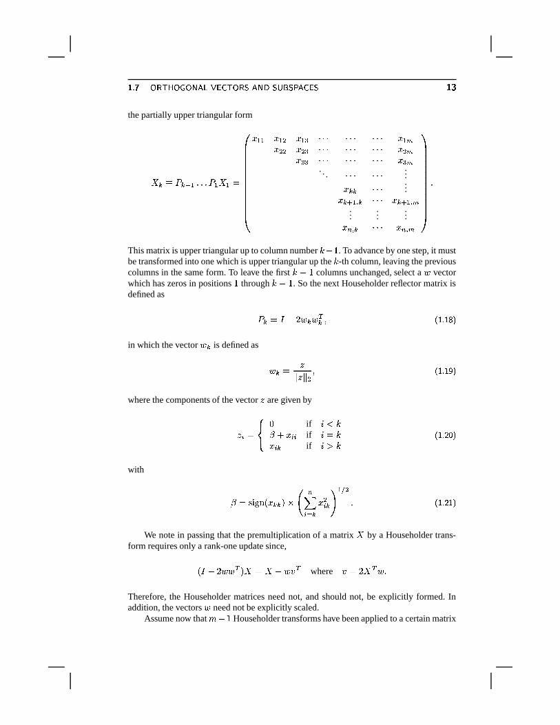
the partially upper triangular form

� � ; � � � �� !""""""""""""#

� �-� � � $ � �� $-$ � $ � �� $ �� . . . �� ...� � � �� ...� � " � � � �� " � � �...

......� � � � ��

&('''''''''''')�

This matrix is upper triangular up to column number � !G� . To advance by one step, it mustbe transformed into one which is upper triangular up the � -th column, leaving the previouscolumns in the same form. To leave the first � !�� columns unchanged, select a � vectorwhich has zeros in positions � through � !�� . So the next Householder reflector matrix isdefined as � � � !�� /� � �� J � �in which the vector � � is defined as

� � � �� $ � �� J � � �where the components of the vector

�are given by� �(� �� % if � � �� q� if �(� �� if � � �

�� J � � �with

� � � � ��*� � � + �� $� � �

�� $� �� J � ��

We note in passing that the premultiplication of a matrix � by a Householder trans-form requires only a rank-one update since,

* � !�� / + � � � ! � � / where � �� / �>�Therefore, the Householder matrices need not, and should not, be explicitly formed. Inaddition, the vectors � need not be explicitly scaled.

Assume now that � ! � Householder transforms have been applied to a certain matrix

� � �� @n K � �;K � � � �� of dimension ~��D� , to reduce it into the upper triangular form,

� � ; � � � � � $��

!"""""""""""#

� � � � � $ � � � �� $ $ �$ � �� $ �� . . ....� � � �%......

&(''''''''''')� �� J � � �

Recall that our initial goal was to obtain a QR factorization of � . We now wish to recoverthe � and # matrices from the � ’s and the above matrix. If we denote by the productof the � on the left-side of (1.22), then (1.22) becomes � � � #� � � �� J � � �in which # is an �� upper triangular matrix, and

�is an * ~ ! � + � � zero block.

Since is unitary, its inverse is equal to its transpose and, as a result,

� � / � #� � � � $^�� #� � �If � � is the matrix of size ~ �� which consists of the first � columns of the identitymatrix, then the above equality translates into

� � / � � # �The matrix � � 2/�� represents the � first columns of / . Since

� / � � � /� / � � � � �� and # are the matrices sought. In summary,

� � ��# �in which # is the triangular matrix obtained from the Householder reduction of � (see(1.22) and (1.23)) and

� � � � � $�� 93/� .8�P��76 &�� */� &�� */��$� � � & &�� &��

1. Define � � � � � ��E�� !2. For � ��[�� Do:3. If � � � compute � � � � � � � � $ �� 4. Compute � � using (1.19), (1.20), (1.21)5. Compute � � � � � � with � � � !�� /�6. Compute � � � � $ �� 7. EndDo

�� (K �� dK � � � �

Note that line 6 can be omitted since the � � are not needed in the execution of thenext steps. It must be executed only when the matrix � is needed at the completion ofthe algorithm. Also, the operation in line 5 consists only of zeroing the components �/��[��E� ~ and updating the � -th component of � � . In practice, a work vector can be used for� � and its nonzero components after this step can be saved into an upper triangular matrix.Since the components 1 through � of the vector � � are zero, the upper triangular matrix #can be saved in those zero locations which would otherwise be unused.

� � ��

{}|��

This section discusses the reduction of square matrices into matrices that have simplerforms, such as diagonal, bidiagonal, or triangular. Reduction means a transformation thatpreserves the eigenvalues of a matrix.

+ �-,/.�01.q�2.4350 �76 �Two matrices � and � are said to be similar if there is a nonsingular

matrix � such that

� � �X�� The mapping � � � is called a similarity transformation.

It is clear that similarity is an equivalence relation. Similarity transformations preservethe eigenvalues of matrices. An eigenvector 8�� of � is transformed into the eigenvector8�) � � 8�� of � . In effect, a similarity transformation amounts to representing the matrix� in a different basis.

We now introduce some terminology.�

An eigenvalue ( of � has algebraic multiplicity � , if it is a root of multiplicity �of the characteristic polynomial.� If an eigenvalue is of algebraic multiplicity one, it is said to be simple. A nonsimpleeigenvalue is multiple.�� The geometric multiplicity � of an eigenvalue ( of � is the maximum number ofindependent eigenvectors associated with it. In other words, the geometric multi-plicity � is the dimension of the eigenspace

� � � * � ! ( � + .� A matrix is derogatory if the geometric multiplicity of at least one of its eigenvaluesis larger than one.

� An eigenvalue is semisimple if its algebraic multiplicity is equal to its geometricmultiplicity. An eigenvalue that is not semisimple is called defective.

Often, ( � � ( $)�� ( � (� � ~ ) are used to denote the distinct eigenvalues of � . It iseasy to show that the characteristic polynomials of two similar matrices are identical; seeExercise 9. Therefore, the eigenvalues of two similar matrices are equal and so are theiralgebraic multiplicities. Moreover, if � is an eigenvector of � , then � � is an eigenvector

� � �� @n K � �;K � � � �� of � and, conversely, if � is an eigenvector of � then � � � � is an eigenvector of � . Asa result the number of independent eigenvectors associated with a given eigenvalue is thesame for two similar matrices, i.e., their geometric multiplicity is also the same.

�� "!#��$

The simplest form in which a matrix can be reduced is undoubtedly the diagonal form.Unfortunately, this reduction is not always possible. A matrix that can be reduced to thediagonal form is called diagonalizable. The following theorem characterizes such matrices.

�P�>� 3/�j�+��76T�A matrix of dimension ~ is diagonalizable if and only if it has ~ line-

arly independent eigenvectors.

�� 6A matrix � is diagonalizable if and only if there exists a nonsingular matrix �

and a diagonal matrix % such that � � �&% � � � , or equivalently � � � ��% , where % isa diagonal matrix. This is equivalent to saying that ~ linearly independent vectors exist —the ~ column-vectors of � — such that � � � �(' � � � . Each of these column-vectors is aneigenvector of � .

A matrix that is diagonalizable has only semisimple eigenvalues. Conversely, if all theeigenvalues of a matrix � are semisimple, then � has ~ eigenvectors. It can be easilyshown that these eigenvectors are linearly independent; see Exercise 2. As a result, wehave the following proposition.

�5�<3/�<32>?.q�2.4350 �76 �A matrix is diagonalizable if and only if all its eigenvalues are

semisimple.

Since every simple eigenvalue is semisimple, an immediate corollary of the above resultis: When � has ~ distinct eigenvalues, then it is diagonalizable.

��*) ��,+-��.�/�0 �/�1��2 � �"!#��$

From the theoretical viewpoint, one of the most important canonical forms of matrices isthe well known Jordan form. A full development of the steps leading to the Jordan formis beyond the scope of this book. Only the main theorem is stated. Details, including theproof, can be found in standard books of linear algebra such as [117]. In the following, � �refers to the algebraic multiplicity of the individual eigenvalue ( � and 3 � is the index of theeigenvalue, i.e., the smallest integer for which

� � � * � ! ( � � + �54 " � �� * � ! ( � � + �64 .�P�>� 3/�j�+��76 �

Any matrix � can be reduced to a block diagonal matrix consisting of� diagonal blocks, each associated with a distinct eigenvalue ( � . Each of these diagonalblocks has itself a block diagonal structure consisting of � � sub-blocks, where � � is thegeometric multiplicity of the eigenvalue ( � . Each of the sub-blocks, referred to as a Jordan

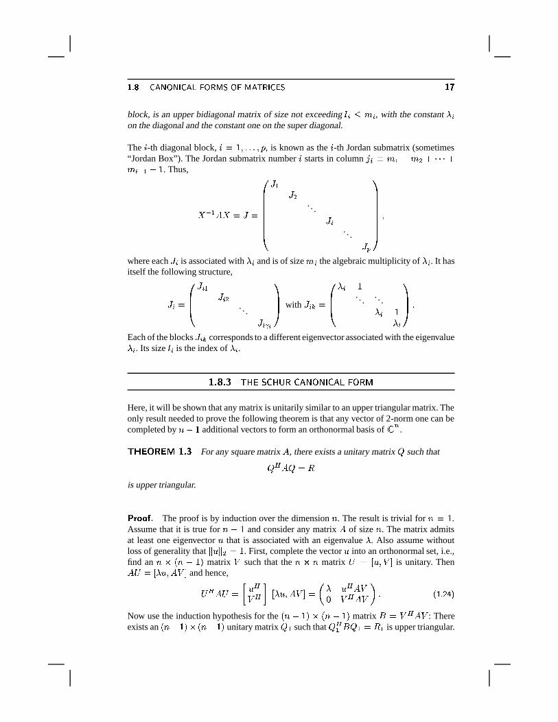
�� (K �� dK � � � �block, is an upper bidiagonal matrix of size not exceeding 3 � � � � , with the constant ( �on the diagonal and the constant one on the super diagonal.

The � -th diagonal block, �:� �[�� , is known as the � -th Jordan submatrix (sometimes“Jordan Box”). The Jordan submatrix number � starts in column �[� ; � � � � $ � ��;�� . Thus,

� � � � � �� !"""""""#

� � ��$. . . �;�

. . . � �

&(''''''')�

where each � � is associated with ( � and is of size � � the algebraic multiplicity of ( � . It hasitself the following structure,

� � � !""#� � � � � $

. . . �;�� 4&('') with � � � �

!""#( � �

. . .. . .( � �

( �

&('') �

Each of the blocks � � � corresponds to a different eigenvector associated with the eigenvalue( � . Its size 3 � is the index of ( � .

��*�� 1��& �/�1��2 � �"!#��$Here, it will be shown that any matrix is unitarily similar to an upper triangular matrix. Theonly result needed to prove the following theorem is that any vector of 2-norm one can becompleted by ~ ! � additional vectors to form an orthonormal basis of � � .

�P�>� 3/�5�� 6 For any square matrix � , there exists a unitary matrix � such that

� 1 � � � #is upper triangular.

�� 6The proof is by induction over the dimension ~ . The result is trivial for ~ � � .

Assume that it is true for ~ ! � and consider any matrix � of size ~ . The matrix admitsat least one eigenvector 8 that is associated with an eigenvalue ( . Also assume withoutloss of generality that

� 8 � $�� . First, complete the vector 8 into an orthonormal set, i.e.,find an ~s� * ~ !O� + matrix � such that the ~s��~ matrix � � 8 � � ! is unitary. Then� � � ($8 � �� ! and hence, 1 � �� 8 1� 1� � (78 � �� ! � � ( 8 1 ��% � 1,�� J � � �Now use the induction hypothesis for the * ~ !�� + � * ~ !�� + matrix � � � 1�� : Thereexists an * ~ ! � + � * ~ !�� + unitary matrix � � such that � 1 � � � � � # � is upper triangular.

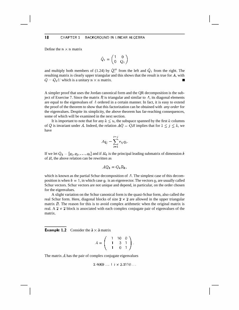
� � �� @n K � �;K � � � �� Define the ~��R~ matrix

�� %% � � �

and multiply both members of (1.24) by ��21� from the left and �� from the right. Theresulting matrix is clearly upper triangular and this shows that the result is true for � , with� � �� which is a unitary ~��D~ matrix.

A simpler proof that uses the Jordan canonical form and the QR decomposition is the sub-ject of Exercise 7. Since the matrix # is triangular and similar to � , its diagonal elementsare equal to the eigenvalues of � ordered in a certain manner. In fact, it is easy to extendthe proof of the theorem to show that this factorization can be obtained with any order forthe eigenvalues. Despite its simplicity, the above theorem has far-reaching consequences,some of which will be examined in the next section.

It is important to note that for any � � ~ , the subspace spanned by the first � columnsof � is invariant under � . Indeed, the relation � � � ��# implies that for � � � �� , wehave

� �<�� F��_�

If we let � � � � � � �� $ �� ! and if # � is the principal leading submatrix of dimension �of # , the above relation can be rewritten as

� � � � � � # � �which is known as the partial Schur decomposition of � . The simplest case of this decom-position is when � �� , in which case � � is an eigenvector. The vectors � � are usually calledSchur vectors. Schur vectors are not unique and depend, in particular, on the order chosenfor the eigenvalues.

A slight variation on the Schur canonical form is the quasi-Schur form, also called thereal Schur form. Here, diagonal blocks of size � � � are allowed in the upper triangularmatrix # . The reason for this is to avoid complex arithmetic when the original matrix isreal. A � � � block is associated with each complex conjugate pair of eigenvalues of thematrix.

� �� 76 � Consider the �M�� matrix

� �!# � � % %

!P� � �!P� % �

&) �

The matrix � has the pair of complex conjugate eigenvalues

�z� � %��`�� F�u�;� % ��

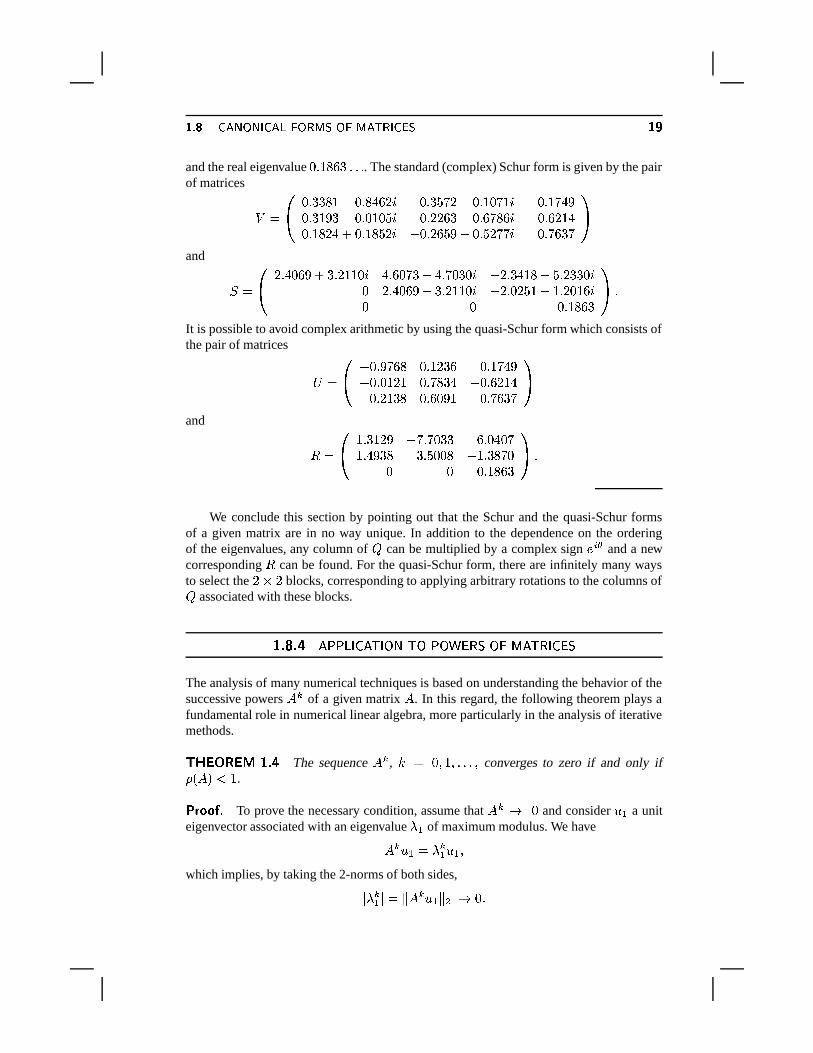
�� (K �� dK � � � �and the real eigenvalue %z�q�� . The standard (complex) Schur form is given by the pairof matrices

� �!# %p� � � �z� ! %z� � � �;�!� %z� �� ! %p�8� % � �� %z�q� � � �%p� � � � � ! %z� %z� % � � !9%p� �;� � � ! %p� � � � �)� !9%z� �;�z� �

%p�8��;� � � %z�q�� !� !9%p� �� ! %p� � � �� %z� � � ��&)

and � � !# �u� � % �� z�[� %[� �p� � % � � ! �� % � %[� !:�u� � �p�� ! � �F� � � %[�% �u� � % �� ! � � �z�[� %[� !:�u� %;� � � ! �[�F��%p� �[�% % %z�q��

&) �

It is possible to avoid complex arithmetic by using the quasi-Schur form which consists ofthe pair of matrices

�!# !9%p� � � �� %z�q�� %z�q� � � �!9%p� %p��z� %z� � � � � !9%z� �;�u� �

%p� �z� � � %z� � % �z� %z� � � ��&)

and

# �!# �;� � �� ! � � � % �� z� % � % ��;� � � � � � � � % %�� !P�[� � � � %% % %z�q��

&) �

We conclude this section by pointing out that the Schur and the quasi-Schur formsof a given matrix are in no way unique. In addition to the dependence on the orderingof the eigenvalues, any column of � can be multiplied by a complex sign �

�and a new

corresponding # can be found. For the quasi-Schur form, there are infinitely many waysto select the � � � blocks, corresponding to applying arbitrary rotations to the columns of� associated with these blocks.

�� 2 �� "��! $ � �� 2 1� �The analysis of many numerical techniques is based on understanding the behavior of thesuccessive powers � � of a given matrix � . In this regard, the following theorem plays afundamental role in numerical linear algebra, more particularly in the analysis of iterativemethods.

�P�>� 3/�5�� 6 �The sequence � � , � � %z��[��#� converges to zero if and only if�* � + � � .

�� 6To prove the necessary condition, assume that � � � % and consider 8 � a unit

eigenvector associated with an eigenvalue ( � of maximum modulus. We have

� � 8 � � ( � � 8 � �which implies, by taking the 2-norms of both sides,

� ( � � � � � � � 8 � � $ � %p�

� � �� @n K � �;K � � � �� This shows that �* � + � � ( � � �3� .

The Jordan canonical form must be used to show the sufficient condition. Assume that�* � + �3� . Start with the equality

� � � � � � � � � �To prove that � � converges to zero, it is sufficient to show that � � converges to zero. Animportant observation is that � � preserves its block form. Therefore, it is sufficient to provethat each of the Jordan blocks converges to zero. Each block is of the form�;�(� ( � � � � �where � � is a nilpotent matrix of index 3 � , i.e., � �� &% . Therefore, for � � 3 � ,� ��

� ��

� � * � !G� + � (� � ��

�� Using the triangle inequality for any norm and taking � � 3 � yields� � ��

� ��

� � * � !\� + �� ( � � � � � � � ��

Since� ( � � � � , each of the terms in this finite sum converges to zero as � � � . Therefore,

the matrix � �� converges to zero.

An equally important result is stated in the following theorem.

�P�>� 3/�j�+��76 � The series �� converges if and only if � * � + � � . Under this condition,

� ! � is nonsingular and the limitof the series is equal to * � ! � + � � .�� 6

The first part of the theorem is an immediate consequence of Theorem 1.4. In-deed, if the series converges, then

� � � � � % . By the previous theorem, this implies that�* � + �3� . To show that the converse is also true, use the equality� ! � � " � � * � ! � + * � �� $ � �� +

and exploit the fact that since �* � + �3� , then� ! � is nonsingular, and therefore,* � ! � + � � * � ! � � " � + � � �� $ � ��

This shows that the series converges since the left-hand side will converge to * � ! � + � � .In addition, it also shows the second part of the theorem.

Another important consequence of the Jordan canonical form is a result that relatesthe spectral radius of a matrix to its matrix norm.

�� @n � �� bK �^K �� dK � � �y��P�>� 3/�5�� 6 �

For any matrix norm� � � , we have

� � �� .� � �* � + �� 6The proof is a direct application of the Jordan canonical form and is the subject

of Exercise 10.

� � ��

{}|��

This section examines specific properties of normal matrices and Hermitian matrices, in-cluding some optimality properties related to their spectra. The most common normal ma-trices that arise in practice are Hermitian or skew-Hermitian.

�� $ � � $ � �� By definition, a matrix is said to be normal if it commutes with its transpose conjugate,i.e., if it satisfies the relation

� 1 � � �� 1 � �� J � � �An immediate property of normal matrices is stated in the following lemma.

�� X� �76T�If a normal matrix is triangular, then it is a diagonal matrix.

�� 6Assume, for example, that � is upper triangular and normal. Compare the first

diagonal element of the left-hand side matrix of (1.25) with the corresponding element ofthe matrix on the right-hand side. We obtain that

� � �-� � $ � �� $ �which shows that the elements of the first row are zeros except for the diagonal one. Thesame argument can now be used for the second row, the third row, and so on to the last row,to show that � �0� �=% for � � � .

A consequence of this lemma is the following important result.

�P�>� 3/�5�� 6 � A matrix is normal if and only if it is unitarily similar to a diagonalmatrix.

�� 6It is straightforward to verify that a matrix which is unitarily similar to a diagonal

matrix is normal. We now prove that any normal matrix � is unitarily similar to a diagonal

�� @n K � �;K � � � �� matrix. Let � � ��#�� 1 be the Schur canonical form of � where � is unitary and # isupper triangular. By the normality of � ,

��# 1 � 1 ��#�� 1 � ��#�� 1 ��# 1 � 1or,

��# 1 #�� 1 � ��# # 1 � 1 �Upon multiplication by � 1 on the left and � on the right, this leads to the equality # 1 # �# #01 which means that # is normal, and according to the previous lemma this is onlypossible if # is diagonal.

Thus, any normal matrix is diagonalizable and admits an orthonormal basis of eigenvectors,namely, the column vectors of � .

The following result will be used in a later chapter. The question that is asked is:Assuming that any eigenvector of a matrix � is also an eigenvector of �21 , is � normal?If � had a full set of eigenvectors, then the result is true and easy to prove. Indeed, if �is the ~�� ~ matrix of common eigenvectors, then �� % � and � 1� � � % $ , with% � and % $ diagonal. Then, �:�01� � � % � % $ and � 1,�� % $ % � and, therefore,�:� 1 � � 1,� . It turns out that the result is true in general, i.e., independently of thenumber of eigenvectors that � admits.

�� X� �76 �A matrix � is normal if and only if each of its eigenvectors is also an

eigenvector of �01 .

�� 6If � is normal, then its left and right eigenvectors are identical, so the sufficient

condition is trivial. Assume now that a matrix � is such that each of its eigenvectors � � , �@��[�� , with � ��~ is an eigenvector of �01 . For each eigenvector � � of � , � � � � ( � � � ,and since � � is also an eigenvector of �01 , then � 1 � � � �� . Observe that * � 1 � � � � � + �� * � � � � � + and because * � 1 � � � � � + � * � � � � � � + � 3( � * � � � � � + , it follows that � � 3( � . Next, itis proved by contradiction that there are no elementary divisors. Assume that the contraryis true for ( � . Then, the first principal vector 8 � associated with ( � is defined by* � ! ( � � + 8 �x� � �2�Taking the inner product of the above relation with � � , we obtain* �98 �6� � � + � ( �-* 8 �2� � � + � * � �6� � � + � �� J � � �On the other hand, it is also true that* �98 � � � � + � * 8 � � � 1 � � + ��* 8 � � 3( � � � + � ( � * 8 � � � � + � �� J �� A result of (1.26) and (1.27) is that * � � � � � + � % which is a contradiction. Therefore, � hasa full set of eigenvectors. This leads to the situation discussed just before the lemma, fromwhich it is concluded that � must be normal.

Clearly, Hermitian matrices are a particular case of normal matrices. Since a normalmatrix satisfies the relation � � ��% � 1 , with % diagonal and � unitary, the eigenvaluesof � are the diagonal entries of % . Therefore, if these entries are real it is clear that � 1 �� . This is restated in the following corollary.

�� @n � �� bK �^K �� dK � � � � 3/�<3 � �Y�>�� 76T�

A normal matrix whose eigenvalues are real is Hermitian.

As will be seen shortly, the converse is also true, i.e., a Hermitian matrix has real eigenval-ues.

An eigenvalue ( of any matrix satisfies the relation

( � * �98 � 8 +* 8 � 8 + �where 8 is an associated eigenvector. Generally, one might consider the complex scalars

� *� + � * � �x�� +*�x�� + � �� J �� defined for any nonzero vector in � � . These ratios are known as Rayleigh quotients andare important both for theoretical and practical purposes. The set of all possible Rayleighquotients as � runs over �t� is called the field of values of � . This set is clearly boundedsince each

�� *� + � is bounded by the the 2-norm of � , i.e.,

�� *� + � � � � � $ for all � .

If a matrix is normal, then any vector � in � � can be expressed as

�� where the vectors � � form an orthogonal basis of eigenvectors, and the expression for � *�� +becomes

� *� + � * � �x�� +*�g�� + � � � �� ( � � � � $� � �� $ ;�� ( � � �� J � � �

where

% � � � � � � � $� � � �� $ � �;� �� [�

From a well known characterization of convex hulls established by Hausdorff (Hausdorff’sconvex hull theorem), this means that the set of all possible Rayleigh quotients as � runsover all of �t� is equal to the convex hull of the ( � ’s. This leads to the following theoremwhich is stated without proof.

�P�>� 3/�5�� 6 �The field of values of a normal matrix is equal to the convex hull of its

spectrum.

The next question is whether or not this is also true for nonnormal matrices and theanswer is no: The convex hull of the eigenvalues and the field of values of a nonnormalmatrix are different in general. As a generic example, one can take any nonsymmetric realmatrix which has real eigenvalues only. In this case, the convex hull of the spectrum isa real interval but its field of values will contain imaginary values. See Exercise 12 foranother example. It has been shown (Hausdorff) that the field of values of a matrix is aconvex set. Since the eigenvalues are members of the field of values, their convex hull iscontained in the field of values. This is summarized in the following proposition.

� � �� @n K � �;K � � � �� 5�<3/�<32>?.q�2.4350 �76 � The field of values of an arbitrary matrix is a convex set whichcontains the convex hull of its spectrum. It is equal to the convex hull of the spectrumwhen the matrix is normal.

��*) ��$ � �/� �/� $ � � ��2 � �A first result on Hermitian matrices is the following.

�P�>� 3/�j�+��76 � The eigenvalues of a Hermitian matrix are real, i.e., : * � + �� .

�� 6Let ( be an eigenvalue of � and 8 an associated eigenvector or 2-norm unity.

Then

( ��* �98 � 8 + � * 8 � �98 + � * �98 � 8 + � ( �which is the stated result.

It is not difficult to see that if, in addition, the matrix is real, then the eigenvectors can bechosen to be real; see Exercise 21. Since a Hermitian matrix is normal, the following is aconsequence of Theorem 1.7.

�P�>� 3/�j�+��76T��Any Hermitian matrix is unitarily similar to a real diagonal matrix.

In particular a Hermitian matrix admits a set of orthonormal eigenvectors that form a basisof �j� .

In the proof of Theorem 1.8 we used the fact that the inner products * �98 � 8 + are real.Generally, it is clear that any Hermitian matrix is such that * � �g�� + is real for any vector� �� . It turns out that the converse is also true, i.e., it can be shown that if * � � � � + isreal for all vectors

�in �t� , then the matrix � is Hermitian; see Exercise 15.

Eigenvalues of Hermitian matrices can be characterized by optimality properties ofthe Rayleigh quotients (1.28). The best known of these is the min-max principle. We nowlabel all the eigenvalues of � in descending order:

( � � ( $ � �� ( � �Here, the eigenvalues are not necessarily distinct and they are repeated, each according toits multiplicity. In the following theorem, known as the Min-Max Theorem, � represents ageneric subspace of � � .

�P�>� 3/�j�+��76T�z�The eigenvalues of a Hermitian matrix � are characterized by the

relation

( � � � � �� " � �� * � �g�� +*�x�� + � �� J � � �

�� @n � �� bK �^K �� dK � � � �� 6

Let � � � �� be an orthonormal basis of � � consisting of eigenvectors of �associated with ( � �� ( � respectively. Let � � be the subspace spanned by the first � ofthese vectors and denote by � * � + the maximum of * � �x�� + � *��g�� + over all nonzero vectorsof a subspace � . Since the dimension of � � is � , a well known theorem of linear algebrashows that its intersection with any subspace � of dimension ~ ! �b� � is not reduced to� % � , i.e., there is vector � in �� . For this �\� � �� , we have* � �x�� +*�x�� + � � �� ( � � � � $� �� $ � ( �so that � * � + � ( � .

Consider, on the other hand, the particular subspace � � of dimension ~ ! �`� � whichis spanned by � � �� . For each vector � in this subspace, we have* � �g�� +*�g�� + � � �� ( � � � � $� �� $ � ( �so that � * � � + � ( � . In other words, as � runs over all the * ~ ! �\� � + -dimensionalsubspaces, � * � + is always � ( � and there is at least one subspace � � for which � * � � + �( � . This shows the desired result.

The above result is often called the Courant-Fisher min-max principle or theorem. As aparticular case, the largest eigenvalue of � satisfies

( � � �� * � �g�� +*�x�� + � �� J � ��Actually, there are four different ways of rewriting the above characterization. The

second formulation is

( � � � � �� * � �g�� +*��g�� + �� J � � �

and the two other ones can be obtained from (1.30) and (1.32) by simply relabeling theeigenvalues increasingly instead of decreasingly. Thus, with our labeling of the eigenvaluesin descending order, (1.32) tells us that the smallest eigenvalue satisfies

( � � � � �� * � �g�� +*��g�� + � �� J � � �with ( � replaced by ( � if the eigenvalues are relabeled increasingly.

In order for all the eigenvalues of a Hermitian matrix to be positive, it is necessary andsufficient that * � �x�� + � %z� �� 5� � � �&%p�Such a matrix is called positive definite. A matrix which satisfies * � �g�� + � % for any � issaid to be positive semidefinite. In particular, the matrix � 1�� is semipositive definite forany rectangular matrix, since* � 1 � �g�� + � * � �x� � � + � %p��g�Similarly, �� 1 is also a Hermitian semipositive definite matrix. The square roots of theeigenvalues of � 1,� for a general rectangular matrix � are called the singular values of

� � �� @n K � �;K � � � �� and are denoted by : � . In Section 1.5, we have stated without proof that the 2-norm ofany matrix � is equal to the largest singular value : � of � . This is now an obvious fact,because � � � $$ � �� $$� � � $$ � � � �� * � �x� � � +*�x�� + � �� * � 1,� �g�� +*�g�� + � : $�which results from (1.31).

Another characterization of eigenvalues, known as the Courant characterization, isstated in the next theorem. In contrast with the min-max theorem, this property is recursivein nature.

�P�>� 3/�j�+��76T� �The eigenvalue ( � and the corresponding eigenvector �� of a Hermi-

tian matrix are such that

( � � * � � � � � � +* � � � � � + � �� * � �g�� +*��g�� +

and for � �3� ,( � � * � � � �� +* � � � � � + � �� * � �g�� +*�x�� + � �� J � � �

In other words, the maximum of the Rayleigh quotient over a subspace that is orthog-onal to the first � ! � eigenvectors is equal to ( � and is achieved for the eigenvector � �associated with ( � . The proof follows easily from the expansion (1.29) of the Rayleighquotient.

�� {b|�{��

Nonnegative matrices play a crucial role in the theory of matrices. They are important inthe study of convergence of iterative methods and arise in many applications includingeconomics, queuing theory, and chemical engineering.

A nonnegative matrix is simply a matrix whose entries are nonnegative. More gener-ally, a partial order relation can be defined on the set of matrices.

+ � , .�01.q�2.43 0 �76 Let � and � be two ~��D� matrices. Then

� � �if by definition, �z�F� �� F� for � � � ��~ , � � � � � . If

�denotes the ~ �D� zero matrix,

then � is nonnegative if � � �, and positive if � � �

. Similar definitions hold in which“positive” is replaced by “negative”.

The binary relation “ � ” imposes only a partial order on �`��z� since two arbitrary matricesin �j��u� are not necessarily comparable by this relation. For the remainder of this section,

�� %� ��^K � � �� dK � ��e � S#� �� dK � � � �we now assume that only square matrices are involved. The next proposition lists a numberof rather trivial properties regarding the partial order relation just defined.

�5�<3/�<32>?.8�1.4350 �76 �The following properties hold.

� The relation � for matrices is reflexive ( � � � ), antisymmetric (if � � � and� � � , then � � � ), and transitive (if � �� and � �� , then � �s� ).� If � and � are nonnegative, then so is their product �� and their sum �� .�� If � is nonnegative, then so is � � .

� If � � � , then � / �� / .

� If� �s� �s� , then

� � � � � � � � � and similarly� � �� .

The proof of these properties is left as Exercise 23.A matrix is said to be reducible if there is a permutation matrix such that P� /

is block upper triangular. Otherwise, it is irreducible. An important result concerning non-negative matrices is the following theorem known as the Perron-Frobenius theorem.

�P�>� 3/�5�� 6T� Let � be a real ~P� ~ nonnegative irreducible matrix. Then ( ;� * � + ,the spectral radius of � , is a simple eigenvalue of � . Moreover, there exists an eigenvector

8 with positive elements associated with this eigenvalue.

A relaxed version of this theorem allows the matrix to be reducible but the conclusion issomewhat weakened in the sense that the elements of the eigenvectors are only guaranteedto be nonnegative.

Next, a useful property is established.

�5�<3/�<32>?.8�1.4350 �76 � Let � � � � � be nonnegative matrices, with � �s� . Then

�,� �s�}� and �N� �s�N� �� 6

Consider the first inequality only, since the proof for the second is identical. Theresult that is claimed translates into

�� <�=� ��~ �which is clearly true by the assumptions.

A consequence of the proposition is the following corollary.

� 3/�<3 � �Y�>�� 76 �Let � and � be two nonnegative matrices, with � � � . Then

� � �� %z� �� J � � �� 6

The proof is by induction. The inequality is clearly true for � � % . Assume that(1.35) is true for � . According to the previous proposition, multiplying (1.35) from the leftby � results in

� � " � � �:� � � �� J � � �

� � �� @n K � �;K � � � �� Now, it is clear that if � � % , then also � � � % , by Proposition 1.6. We now multiply bothsides of the inequality � �� by � � to the right, and obtain

�:� � � � � " � � �� J �� The inequalities (1.36) and (1.37) show that � � " � �s� � " � , which completes the inductionproof.

A theorem which has important consequences on the analysis of iterative methods willnow be stated.

�P�>� 3/�j�+��76T� �Let � and � be two square matrices that satisfy the inequalities

� �s� �s� � �� J �� Then

�* � + � �* � + � �� J � � �� 6

The proof is based on the following equality stated in Theorem 1.6� * � + � � � �� .�

for any matrix norm. Choosing the � ! norm, for example, we have from the last propertyin Proposition 1.6

� * � + � � � �� .�� * � +which completes the proof.

�P�>� 3/�j�+��76T� � Let � be a nonnegative matrix. Then � * � + �� if and only if� ! �

is nonsingular and * � ! � + � � is nonnegative.

�� 6Define � � � ! � . If it is assumed that � * � + � � , then by Theorem 1.5,� � � ! � is nonsingular and

� � � � * � ! � + � � �� J � � �

In addition, since � � % , all the powers of � as well as their sum in (1.40) are alsononnegative.

To prove the sufficient condition, assume that � is nonsingular and that its inverseis nonnegative. By the Perron-Frobenius theorem, there is a nonnegative eigenvector 8associated with �* � + , which is an eigenvalue, i.e.,

�18 � � * � + 8or, equivalently,

� � � 8 � �� ! �* � + 8 �

Since 8 and �5� � are nonnegative, and� ! � is nonsingular, this shows that �?! � * � + � % ,

which is the desired result.

�� %� ��^K � � �� dK � ��e � S#� �� dK � � � �+ �-,/.�01.q�2.4350 �76 �

A matrix is said to be an � -matrix if it satisfies the following fourproperties:

� � � � � � % for ��O�;��E� ~ .� �� % for � ��;�x�<�=�}��;��E� ~ .�� is nonsingular.� �2� � � % .

In reality, the four conditions in the above definition are somewhat redundant andequivalent conditions that are more rigorous will be given later. Let � be any matrix whichsatisfies properties (1) and (2) in the above definition and let % be the diagonal of � . Since% � % ,

� � % ! * % ! � + � %�� ! * � ! % � � � + � �Now define

� ;� ! % � � � �

Using the previous theorem,� ! � � % � � � is nonsingular and * � ! � + � � � �1� � % � %

if and only if � * � + �� . It is now easy to see that conditions (3) and (4) of Definition 1.4can be replaced by the condition � * � + � � .�P�>� 3/�5�� 6T� �

Let a matrix � be given such that� �� % for ��O�;��E� ~ .� �� % for � ��;�x�<�=�}��;��E� ~ .

Then � is an � -matrix if and only if�� * � + � � , where � � � ! % � � � .

�� 6From the above argument, an immediate application of Theorem 1.15 shows that

properties (3) and (4) of the above definition are equivalent to � * � + � � , where � � � ! �and � � % � � � . In addition, � is nonsingular iff � is and � � � is nonnegative iff � is.

The next theorem shows that the condition (1) in Definition 1.4 is implied by the otherthree.

�P�>� 3/�5�� 6T� � Let a matrix � be given such that� �� % for � ��;�x�<�=�}��;��E� ~ .� � is nonsingular.�� 2� � � % .

Then� � � � � � % for ��O�;��E� ~ , i.e., � is an � -matrix.� �* � + � � where � � � ! % � � � .

� �� @n K � �;K � � � �� 6

Define � ; �1� � . Writing that * �� + �8� �O� yields

�� which gives

� �q� � �q� �� ! �� 4

� � � � � � �Since � � � � � � � % for all � , the right-hand side is � � and since � �8� � % , then � �8� � % .The second part of the result now follows immediately from an application of the previoustheorem.

Finally, this useful result follows.

�P�>� 3/�j�+��76T� �Let � � � be two matrices which satisfy

�� s� .�� 0� � % for all � �� .

Then if � is an � -matrix, so is the matrix � .

�� 6Assume that � is an � -matrix and let %�� denote the diagonal of a matrix � .

The matrix % � is positive because

% � � % ) � %p�Consider now the matrix

� ! % � �� . Since � �s� , then

% ) ! � � % � ! � � �

which, upon multiplying through by % � �) , yields� ! % � �) � � % � �) * % � ! � + � % � �� * % � ! � + � � ! % � �� Since the matrices

� ! % � �� and� ! % � �) � are nonnegative, Theorems 1.14 and 1.16

imply that�* � ! % � �� + � �* � ! % � �) � + �3�[�

This establishes the result by using Theorem 1.16 once again.

�� (� � �� {b|�{>{

A real matrix is said to be positive definite or positive real if* � 8 � 8 + � %z� � 8�� j� � 8 � %p� �� J � � �

�� pK �^K �)S2n ��K �@K � � �� dK � � �

It must be emphasized that this definition is only useful when formulated entirely for realvariables. Indeed, if 8 were not restricted to be real, then assuming that * �98 � 8 + is realfor all 8 complex would imply that � is Hermitian; see Exercise 15. If, in addition toDefinition 1.41, � is symmetric (real), then � is said to be Symmetric Positive Definite(SPD). Similarly, if � is Hermitian, then � is said to be Hermitian Positive Definite (HPD).Some properties of HPD matrices were seen in Section 1.9, in particular with regards

to their eigenvalues. Now the more general case where � is non-Hermitian and positivedefinite is considered.

We begin with the observation that any square matrix (real or complex) can be decom-posed as

� �� J � � �in which

� � �� * �� 1 + �� J � � �� )� * � ! � 1 + � �� J � � �

Note that both � and � are Hermitian while the matrix � � in the decomposition (1.42)is skew-Hermitian. The matrix � in the decomposition is called the Hermitian part of� , while the matrix � � is the skew-Hermitian part of � . The above decomposition is theanalogue of the decomposition of a complex number

�into

� � � � � � ,

�R�� %* � + � �� * � � 3� + � �/�� * � + � �

�!� * � ! 3� + �When � is real and 8 is a real vector then * �98 � 8 + is real and, as a result, the decom-

position (1.42) immediately gives the equality* � 8 � 8 + ��*�� 8 � 8 + � �� J � � �This results in the following theorem.

�P�>� 3/�5�� 6T� � Let � be a real positive definite matrix. Then � is nonsingular. Inaddition, there exists a scalar � � % such that* � 8 � 8 + � � � 8 � $$ � �� J � � �for any real vector 8 .

�� 6The first statement is an immediate consequence of the definition of positive defi-

niteness. Indeed, if � were singular, then there would be a nonzero vector such that �98 �=%and as a result * � 8 � 8 + � % for this vector, which would contradict (1.41). We now provethe second part of the theorem. From (1.45) and the fact that � is positive definite, weconclude that � is HPD. Hence, from (1.33) based on the min-max theorem, we get

� � �� * � 8 � 8 +* 8 � 8 + � � � �

� �� *�� 8 � 8 +* 8 � 8 + � ( � � � *�� + � %z�Taking � ; ( � � � *�� + yields the desired inequality (1.46).

A simple yet important result which locates the eigenvalues of � in terms of the spectra

� �� @n K � �;K � � � �� of � and � can now be proved.

�P�>� 3/�j�+��76 � �Let � be any square (possibly complex) matrix and let �� $ * �s�� 1 + and � � �$ � * � ! � 1 + . Then any eigenvalue ( � of � is such that

( � � � *�� + � � �%* ( � + � ( �� *�� + �� J � � �( � � � * � + � � � * ( � + � ( �� * � + � �� J � �

�� 6When the decomposition (1.42) is applied to the Rayleigh quotient of the eigen-

vector 8 � associated with ( � , we obtain

( � � * �98 � � 8 � + � *�� 8 � � 8 � + � ��* �?8 � � 8 � + � �� J � � �assuming that

� 8 � � $ �� . This leads to

� �%* ( � + � *�� 8 � � 8 � +� � * ( � + � * �?8 �[� 8 � + �The result follows using properties established in Section 1.9.

Thus, the eigenvalues of a matrix are contained in a rectangle defined by the eigenval-ues of its Hermitian part and its non-Hermitian part. In the particular case where � is real,then � � is skew-Hermitian and its eigenvalues form a set that is symmetric with respect tothe real axis in the complex plane. Indeed, in this case, � � is real and its eigenvalues comein conjugate pairs.

Note that all the arguments herein are based on the field of values and, therefore,they provide ways to localize the eigenvalues of � from knowledge of the field of values.However, this approximation can be inaccurate in some cases.

� �� 76 Consider the matrix

� � � � �� %�� The eigenvalues of � are ! � � and 101. Those of � are � � *_� % � � � + � � and those of � �are ��*_� %�� ! � + � � .

When a matrix � is Symmetric Positive Definite, the mapping

�x�� *�x�� + � ;* � �g�� + �� J � � �

from �j�l��j� to � is a proper inner product on � � , in the sense defined in Section 1.4.The associated norm is often referred to as the energy norm. Sometimes, it is possible tofind an appropriate HPD matrix � which makes a given matrix � Hermitian, i.e., such that* � �g�� + � ��*�x� � � + � �� g��although � is a non-Hermitian matrix with respect to the Euclidean inner product. Thesimplest examples are � � �� and � � �N� , where � is Hermitian and � is HermitianPositive Definite.

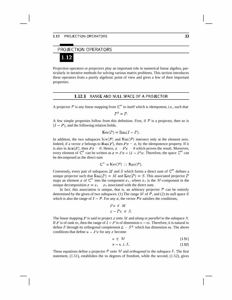
�� ^K �� $

� �� {b|E{ �

Projection operators or projectors play an important role in numerical linear algebra, par-ticularly in iterative methods for solving various matrix problems. This section introducesthese operators from a purely algebraic point of view and gives a few of their importantproperties.

�� )�� /�1��,�/�� ! � ��+ � ��

A projector is any linear mapping from � � to itself which is idempotent, i.e., such that $ � �A few simple properties follow from this definition. First, if is a projector, then so is* � ! + , and the following relation holds,� � � * + � � ��* � ! + �In addition, the two subspaces

� � � * + and

��* + intersect only at the element zero.

Indeed, if a vector � belongs to

��* + , then �G� � , by the idempotence property. If it

is also in

� � � * + , then � ��% . Hence, �X� � ��% which proves the result. Moreover,every element of �j� can be written as �G� � � * � ! + � . Therefore, the space � � canbe decomposed as the direct sum

�j� �� * + � �

��* + �Conversely, every pair of subspaces � and � which forms a direct sum of �,� defines aunique projector such that

��* + � � and

� � � * + � � . This associated projector maps an element � of � � into the component � � , where � � is the � -component in theunique decomposition �R� � � � � $ associated with the direct sum.

In fact, this association is unique, that is, an arbitrary projector can be entirelydetermined by the given of two subspaces: (1) The range � of , and (2) its null space �which is also the range of

� ! . For any � , the vector � satisfies the conditions, � � �� ! � � � �

The linear mapping is said to project � onto � and along or parallel to the subspace � .If is of rank � , then the range of

� ! is of dimension ~ ! � . Therefore, it is natural todefine � through its orthogonal complement � � �� which has dimension � . The aboveconditions that define 8 � � for any � become

8 � � �� J � �� ! 8�� J � � �

These equations define a projector onto � and orthogonal to the subspace � . The firststatement, (1.51), establishes the � degrees of freedom, while the second, (1.52), gives

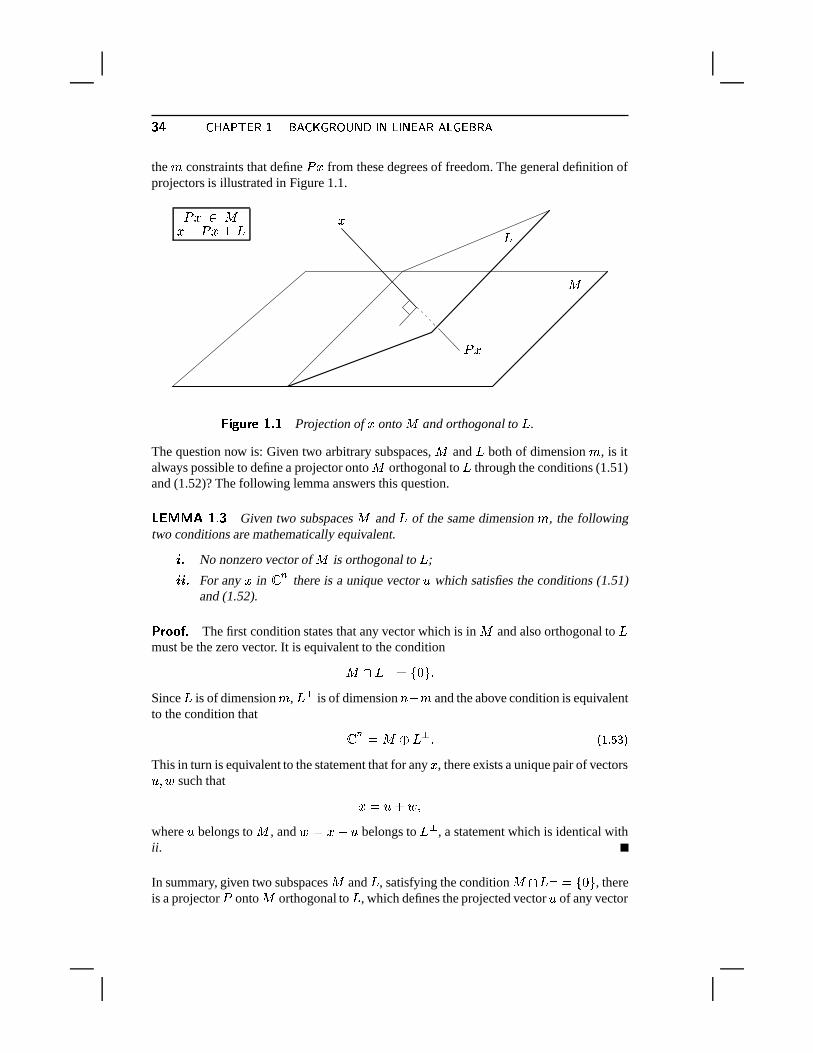
� �� @n K � �;K � � � �� the � constraints that define � from these degrees of freedom. The general definition ofprojectors is illustrated in Figure 1.1.

�

�

�

�

� � �� ! � ��

, � �� 76T� Projection of � onto � and orthogonal to � .

The question now is: Given two arbitrary subspaces, � and � both of dimension � , is italways possible to define a projector onto � orthogonal to � through the conditions (1.51)and (1.52)? The following lemma answers this question.

�� X� �76 Given two subspaces � and � of the same dimension � , the followingtwo conditions are mathematically equivalent.

� No nonzero vector of � is orthogonal to � ;

�� For any � in �j� there is a unique vector 8 which satisfies the conditions (1.51)and (1.52).

�� 6The first condition states that any vector which is in � and also orthogonal to �

must be the zero vector. It is equivalent to the condition

�� % � �Since � is of dimension � , � � is of dimension ~ ! � and the above condition is equivalentto the condition that

�5� � � � � � � �� J � � �This in turn is equivalent to the statement that for any � , there exists a unique pair of vectors8 � � such that

�\� 8/� �>�where 8 belongs to � , and �3� � ! 8 belongs to � � , a statement which is identical withii.

In summary, given two subspaces � and � , satisfying the condition �� % � , thereis a projector onto � orthogonal to � , which defines the projected vector 8 of any vector

�� ^K ��

� from equations (1.51) and (1.52). This projector is such that��* + � � � � � � * + � � � �

In particular, the condition �\� % translates into � � � � � * + which means that � � � � .The converse is also true. Hence, the following useful property, �R�=% iff � � � � �� J � � �

�� )��) $ � �� /�2�� Two bases are required to obtain a matrix representation of a general projector: a basis� � � � � �� ! for the subspace � �

��* + and a second one � � � � � �� !for the subspace � . These two bases are biorthogonal when* � �+� �L� + �=��0�[� �� J � � �

In matrix form this means � 1 � � �. Since � belongs to � , let � � be its representation

in the � basis. The constraint � ! � � � is equivalent to the condition,* *�� ! � � + � �L� + � % for �}��[��E� � �In matrix form, this can be rewritten as

� 1 *� ! � � + �&%z� �� J � � �If the two bases are biorthogonal, then it follows that � � � 1 � . Therefore, in this case, �R� �� 1 � , which yields the matrix representation of , � �� 1 � �� J �� In case the bases � and � are not biorthogonal, then it is easily seen from the condition(1.56) that � � * � 1 � + � � � 1 � �� J �� If we assume that no vector of � is orthogonal to � , then it can be shown that the � �R�matrix � 1 � is nonsingular.

�� )�� 1�/�� /��0�� + � �� An important class of projectors is obtained in the case when the subspace � is equal to� , i.e., when � � � * + � � ��* + � �Then, the projector is said to be the orthogonal projector onto � . A projector that isnot orthogonal is oblique. Thus, an orthogonal projector is defined through the followingrequirements satisfied for any vector � , � � � �� * � ! + � � � �� J � � �

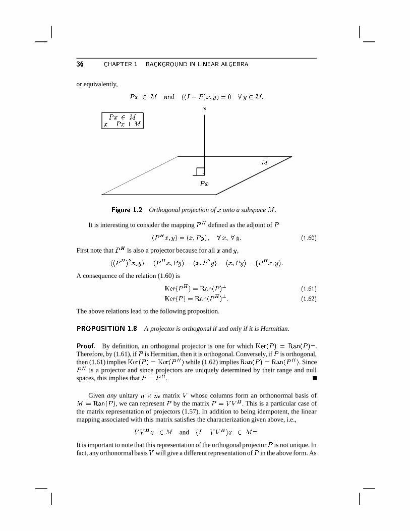
� �� @n K � �;K � � � �� or equivalently, � � � �� * * � ! + �x�� + �&% � � � � �

� �

�

�

� � �� ! � � �

, � �� 76 � Orthogonal projection of � onto a subspace � .

It is interesting to consider the mapping 1 defined as the adjoint of * 1 �x�� + � *��g� � + � � �x� ��y� �� J � � �First note that 1 is also a projector because for all � and � ,* * 1 + $ �x�� + ��* 1 �g� � + ��*�x� $ � + � *�x� � + ��* 1 �g�� + �A consequence of the relation (1.60) is� � � * 1 + � � ��* + � �� J � � �� * + � � ��* 1 + � � �� J � � �The above relations lead to the following proposition.

�5�<3/�<32>?.q�2.4350 �76 �A projector is orthogonal if and only if it is Hermitian.

�� 6By definition, an orthogonal projector is one for which

� � � * + � ��* + � .

Therefore, by (1.61), if is Hermitian, then it is orthogonal. Conversely, if is orthogonal,then (1.61) implies

� � � * + � � � � * 1 + while (1.62) implies

��* + � � ��* 1 + . Since 21 is a projector and since projectors are uniquely determined by their range and null

spaces, this implies that � 1 .

Given any unitary ~3� � matrix � whose columns form an orthonormal basis of� �

��* + , we can represent by the matrix � � � 1 . This is a particular case of

the matrix representation of projectors (1.57). In addition to being idempotent, the linearmapping associated with this matrix satisfies the characterization given above, i.e.,� � 1 � � � and * � ! � � 1 + � � � � �It is important to note that this representation of the orthogonal projector is not unique. Infact, any orthonormal basis � will give a different representation of in the above form. As

�� ^K �� a consequence for any two orthogonal bases � � � � $ of � , we must have � � � 1� � � $ � 1$ ,an equality which can also be verified independently; see Exercise 26.

�� )�� /�*� � � ! �� 1�/�� + � �� When is an orthogonal projector, then the two vectors � and * � ! + � in the decom-position �R� � � * � ! + � are orthogonal. The following relation results:� � � $$ � � � � $$ � � * � ! + � � $$ �A consequence of this is that for any � ,� � � $ � � � � $)�Thus, the maximum of

� � � $ � � � � $ , for all � in �j� does not exceed one. In addition thevalue one is reached for any element in

��* + . Therefore,� � $`��

for any orthogonal projector .An orthogonal projector has only two eigenvalues: zero or one. Any vector of the range

of is an eigenvector associated with the eigenvalue one. Any vector of the null-space isobviously an eigenvector associated with the eigenvalue zero.

Next, an important optimality property of orthogonal projectors is established.

�P�>� 3/�5�� 6 �y�Let be the orthogonal projector onto a subspace � . Then for any

given vector � in �j� , the following is true:� � �� ! � � $:� � � ! � � $)� �� J � � �

�� 6Let � be any vector of � and consider the square of its distance from � . Since� ! � is orthogonal to � to which � ! � belongs, then� � ! � � $$ � � � ! � � * � ! � + � $$ � � � ! � � $$ � � * � ! � + � $$ �

Therefore,� � ! � � $ � � ��! � � $ for all � in � . This establishes the result by noticing

that the minimum is reached for �Z� � .

By expressing the conditions that define � ; � for an orthogonal projector onto

a subspace � , it is possible to reformulate the above result in the form of necessary andsufficient conditions which enable us to determine the best approximation to a given vector� in the least-squares sense.

� 3/�<3 � �Y�>�� 76 Let a subspace � , and a vector � in �`� be given. Then� � �� ! � � $ � � � ! � � $ � �� J � � �

if and only if the following two conditions are satisfied,� � � �� ! � � � �

� �� @n K � �;K � � � �� {b|�{ �

Linear systems are among the most important and common problems encountered in scien-tific computing. From the theoretical point of view, the problem is rather easy and explicitsolutions using determinants exist. In addition, it is well understood when a solution ex-ists, when it does not, and when there are infinitely many solutions. However, the numericalviewpoint is far more complex. Approximations may be available but it may be difficult toestimate how accurate they are. This clearly will depend on the data at hand, i.e., primarilyon the coefficient matrix. This section gives a very brief overview of the existence theoryas well as the sensitivity of the solutions.

�� /� � ��1 1�"� ! � � � � ��Consider the linear system

� �R� � � �� J � � �Here, � is termed the unknown and � the right-hand side. When solving the linear system(1.65), we distinguish three situations.

Case 1 The matrix � is nonsingular. There is a unique solution given by �R� � � � � .Case 2 The matrix � is singular and � � � ��* � + . Since � � � ��* � + , there is an � �such that � � � � � . Then � � � � is also a solution for any � in

� � � * � + . Since

� � � * � + isat least one-dimensional, there are infinitely many solutions.

Case 3 The matrix � is singular and � �� * � + . There are no solutions.

� �� 76 � The simplest illustration of the above three cases is with small diagonalmatrices. Let

� � � � %% � � � �

� ��

Then � is nonsingular and there is a unique � given by

�R� � %p� �� Now let

� � � � %% % � � � �

� �%��

Then � is singular and, as is easily seen, �2� ��* � + . For example, a particular element� � such that � � � � � is � � � � � � �� . The null space of � consists of all vectors whose first

component is zero, i.e., all vectors of the form � �� . Therefore, there are infinitely many

�� K � �� DK � �;K � � � �� 7� � ��solution which are given by

� * � + �� %p� �� 5�

Finally, let � be the same as in the previous case, but define the right-hand side as

� ��

In this case there are no solutions because the second equation cannot be satisfied.

�� ) �� /�2�� /� � �� Consider the linear system (1.65) where � is an ~��j~ nonsingular matrix. Given any matrix� , the matrix � *�� + � � � � � is nonsingular for � small enough, i.e., for � � � where � issome small number; see Exercise 32. Assume that we perturb the data in the above system,i.e., that we perturb the matrix � by � � and the right-hand side � by � � . The solution ��*�� +of the perturbed system satisfies the equation,* �� + � *�� + � �@� � �Y� �� J � � �Let � *�� + �� *�� + ! � . Then,* �� + � *�� + ��* �� + ! * �� + �� * �9! � � +� *�� + �� * �� + � � * �9! � � + �As an immediate result, the function � *�� + is differentiable at �?� % and its derivative isgiven by

�� *�% + � � � ��

� *�� +� � � � � * �9! � � + � �� J �� The size of the derivative of ��*�� + is an indication of the size of the variation that the solu-tion ��*�� + undergoes when the data, i.e., the pair � � � � ! is perturbed in the direction � � � � ! .In absolute terms, a small variation � � � �� ! will cause the solution to vary by roughly�� * % + �� * � ! � � + . The relative variation is such that� � *�� + ! � �� >� � � � � �� *�� + �Using the fact that

� � � � � � � � � � in the above equation yields� ��*�� + ! � �� *�� + �� J �� which relates the relative variation in the solution to the relative sizes of the perturbations.The quantity

��* � + � � � � � � � � �

� � �� @n K � �;K � � � �� is called the condition number of the linear system (1.65) with respect to the norm

� � � . Thecondition number is relative to a norm. When using the standard norms

� � � � , � ��;��E� � ,it is customary to label ��* � + with the same label as the associated norm. Thus,

� � * � + � � � � � � � � � � � �For large matrices, the determinant of a matrix is almost never a good indication of

“near” singularity or degree of sensitivity of the linear system. The reason is that�� * � + is

the product of the eigenvalues which depends very much on a scaling of a matrix, whereasthe condition number of a matrix is scaling-invariant. For example, for � � � � the deter-minant is

�� * � + �� , which can be very small if� � � �3� , whereas ��* � + �� for any of

the standard norms.In addition, small eigenvalues do not always give a good indication of poor condition-

ing. Indeed, a matrix can have all its eigenvalues equal to one yet be poorly conditioned.

� �� 76 � The simplest example is provided by matrices of the form

� � �� /�

for large � . The inverse of � � is

� � �� ! �� /�and for the � -norm we have � � � �� O� � � � �so that

� � * � � + ��*_� � � � � + $ �For a large � , this can give a very large condition number, whereas all the eigenvalues of� � are equal to unity.

When an iterative procedure is used for solving a linear system, we typically face theproblem of choosing a good stopping procedure for the algorithm. Often a residual norm,� � � � � � ! �� is available for some current approximation �� and an estimate of the absolute error

� �9!��

or the relative error� � !

�� is desired. The following simple relation is helpful in this

regard, � � !�� * � + � � ��

It is necessary to have an estimate of the condition number ��* � + in order to exploit theabove relation.

� �� gK � � � �@n � � � � � �

� � ��

1 Verify that the Euclidean inner product defined by (1.4) does indeed satisfy the general definitionof inner products on vector spaces.

2 Show that two eigenvectors associated with two distinct eigenvalues are linearly independent.In a more general sense, show that a family of eigenvectors associated with distinct eigenvaluesforms a linearly independent family.

3 Show that if � is any nonzero eigenvalue of the matrix �� , then it is also an eigenvalue of thematrix �� . Start with the particular case where � and � are square and � is nonsingular, thenconsider the more general case where �� may be singular or even rectangular (but such that�� and �� are square).

4 Let � be an �� orthogonal matrix, i.e., such that �� , where � is a diagonal matrix.Assuming that � is nonsingular, what is the inverse of � ? Assuming that �� , how can � betransformed into a unitary matrix (by operations on its rows or columns)?

5 Show that the Frobenius norm is consistent. Can this norm be associated to two vector normsvia (1.7)? What is the Frobenius norm of a diagonal matrix? What is the � -norm of a diagonalmatrix (for any � )?

6 Find the Jordan canonical form of the matrix:

��! � � ��"� � �$#

Same question for the matrix obtained by replacing the element %'&(& by 1.

7 Give an alternative proof of Theorem 1.3 on the Schur form by starting from the Jordan canonicalform. [Hint: Write �)��*,+-*/.10 and use the QR decomposition of * .]

8 Show from the definition of determinants used in Section 1.2 that the characteristic polynomialis a polynomial of degree for an ��2 matrix.

9 Show that the characteristic polynomials of two similar matrices are equal.

10 Show that 35456798�: ; � 7 ; 0=< 7 �)>@?A�CBD�

for any matrix norm. [Hint: Use the Jordan canonical form.]

11 Let * be a nonsingular matrix and, for any matrix norm; # ; , define

; � ;FE � ; ��* ; . Showthat this is indeed a matrix norm. Is this matrix norm consistent? Show the same for

; *G� ; and;IH ��* ; whereH

is also a nonsingular matrix. These norms are not, in general, associated withany vector norms, i.e., they can’t be defined by a formula of the form (1.7). Why? What aboutthe particular case

; � ;DJ � ; *K��*�.10 ; ?12 Find the field of values of the matrix

�� L� �

and verify that it is not equal to the convex hull of its eigenvalues.

� � �� @n K � �;K � � � �� 13 Show that for a skew-Hermitian matrix � ,

�� ?�� @B �� for any �� #14 Given an arbitrary matrix � , show that if ?��1��@B �� for all � in � , then it is true that

?�� B��?�� 'B �� #[Hint: Expand ?�� ?�� BD�� B .]

15 Using the results of the previous two problems, show that if ?A� � �� B is real for all � in !� ,then � must be Hermitian. Would this result be true if the assumption were to be replaced by:?A�"�1��@B is real for all real � ? Explain.

16 The definition of a positive definite matrix is that ?A�"�1��@B be real and positive for all real vectors� . Show that this is equivalent to requiring that the Hermitian part of � , namely, 0# ?A�� C��B ,be (Hermitian) positive definite.

17 Let � 0 � � . 0%$ and � # �&$ � where $ is a Hermitian matrix and � is a Hermitian PositiveDefinite matrix. Are � 0 and � # Hermitian in general? Show that � 0 and � # are Hermitian(self-adjoint) with respect to the � -inner product.

18 Let a matrix � be such that � � � � ?A�CB where � is a polynomial. Show that � is normal. [Hint:Use Lemma 1.2.]

19 Show that � is normal iff its Hermitian and skew-Hermitian parts, as defined in Section 1.11,commute.

20 Let � be a Hermitian matrix and � a Hermitian Positive Definite matrix defining a � -innerproduct. Show that � is Hermitian (self-adjoint) with respect to the � -inner product if and onlyif � and � commute. What condition must satisfy � for the same condition to hold in the moregeneral case where � is not Hermitian?

21 Let � be a real symmetric matrix and � an eigenvalue of � . Show that if ' is an eigenvectorassociated with � , then so is (' . As a result, prove that for any eigenvalue of a real symmetricmatrix, there is an associated eigenvector which is real.

22 Show that a Hessenberg matrix ) such that *,+.- 0�/ +10�� 32�� #9#9# �� /� , cannot be deroga-tory.

23 Prove all the properties listed in Proposition 1.6.

24 Let � be an 4 -matrix and ' ��5 two nonnegative vectors such that 576 � . 0 '98 �. Show that� � ':5 6 is an 4 -matrix.

25 Show that if ;=<)�&<)� then ;=< ��61�&<)�>6 � . Conclude that under the same assumption,we have

; � ; # < ; � ; # .26 Show that for two orthogonal bases ? 0 �@? # of the same subspace 4 of � we have ? 0 ? �0 �K�? # ?�# �1�A�� .

27 What are the eigenvalues of a projector? What about its eigenvectors?

28 Show that if two projectors B 0 and B # commute, then their product B��=B 0 B # is a projector.What are the range and kernel of B ?

� �� gK � � � �@n � � � � �

29 Consider the matrix � of size � and the vector � � � � ,

��

!""""""#

�L��"��"�� #9#9# �� "�� #9#9# �� #9#9# ��...

......

. . ....

......

......

. . ....� � � #9#9# � �

& '''''') � �

!"""""#

�� ...�� . 0

& ''''') #

�� Compute � � ,; � � ; # , and

; � ; # . � Show that; � ; #� � .

�� Give a lower bound for � # ?A� B .30 What is the inverse of the matrix � of the previous exercise? Give an expression of � 0 ?A� B and

� : ?A�CB based on this.

31 Find a small rank-one perturbation which makes the matrix � in Exercise 29 singular. Derive alower bound for the singular values of � .

32 Consider a nonsingular matrix � . Given any matrix � , show that there exists � such that thematrix ��?��IB � � � �� is nonsingular for all � 8�� . What is the largest possible value for �satisfying the condition? [Hint: Consider the eigenvalues of the generalized eigenvalue problem� ' �� ' .]

NOTES AND REFERENCES. For additional reading on the material presented in this chapter, seeGolub and Van Loan [108], Datta [64], Stewart [202], and Varga [213]. Details on matrix eigenvalueproblems can be found in Gantmacher’s book [100] and Wilkinson [227]. An excellent treatise ofnonnegative matrices is in the book by Varga [213] which remains a good reference on iterativemethods more three decades after its first publication. Another book with state-of-the-art coverageon iterative methods up to the very beginning of the 1970s is the book by Young [232] which covers4 -matrices and related topics in great detail. For a good overview of the linear algebra aspects ofmatrix theory and a complete proof of Jordan’s canonical form, Halmos [117] is recommended.

� � � � � � �

�

��

�;��&0"2� �!9cn(� op$�&8$�-#"_� �!9�[aYC��#"2� .[-E� � �cn )� � �+.;-E�k"2� "6C#"%$}B6VP4i��&("6��$}B�� '�'A$+�="t�H.;C!&8�<$.�4L�+ ��&I�%$MQj�#"+&T� UR �&I.[B!9 $�QL�<J ��$P"wV! �� <�)9Y1g�+V/"H.Z�=.;9 *�$>�+C��/$<aYC��#"2� .[-E�N� �t"H.�� "+��$�Q:e!�IJ $�J0eA"H.`�! ! �&I.<UA�0Q5�E"H$�"6��$�QsB6Vt$<aYC��#"2� .;-E�d"+��#"(�0-#*E.;9 *�$L�jfz-�� "H$-!C!Q`B�$�&;.�4hC!-!]�-E.#1L-E�<J ��$tQj�#"+&T� U� �&I.[B!9 $�QL�d"+��#"h��&T� �%$@4=&I.;Ql"6��$+�%$^W[� �%��&q$2"2� m+�ES"_� .;-E�c��&q$�'�$�-�$�&8�)9 9 V`9 ��&I'A$��!-�W`�6 ��&8�H$�e)�IJ $�J0e�"+��$6V`��#*�$(*�$�&0Vj4i$21�-E.;-Em+$�&I.�$�-#"+&T� $+�<J��$�&8$b��&q$>�%$6*�$�&q�!9dW[� op$�&8$�-#" 1g�+VE��"=.RW[� �%��&8$6"2� m<$>� �Y��&0"_� �)9gn(� op$�&8$�-#"_� �!9�[aYC��ES"_� .;-)J ��$L�2�FQ: !9 $+�="�Q5$6"+�E.)WPCE�%$+�� ) ! �&I.#UA�FQj�#"2� .;-E�c4T.!&�"6��$t ��&IS"_� �!9AW[� op$�&q$�-#"2� �!9�.[ A$�&q�#"H.!&I�<J �^��$�� "!#�� %$'&(� &8$� !9 ��<$+�("6��$j.!&i� ')�0-��!94kC!-��6"2� .;-tB6VL�^4kC!-��6"2� .[-@1L�� E�c�H.;Q5$�W!$+'[&8$<$@.�4u�6Q5.!.�"+�!-�$+�=�g.�*�$�&["+��$('[9 .;B��!9WA.[Q5�A�0-)edB!C#"t1L�� M� �N �� $<�<$61�� %$M �.;9 V!-E.[Q � �)9u.[-b�2�0Q` !9 $P�<$�9 9 �<ep�+C��/��`�+Q5�!9 9"6&T� �)-E'[9 $+�@.!&@&8$<�2"%�!-E';9 $+�+J �� tQ5$6"+�E.)W/� �t �&I.[B��)B!9 V`"6��$,Q5.��="^'A$�-�$�&8�)9;�!-�W,1g$�9 9C!-�W!$�&8�k"H.!.)WbW[� �%��&8$6"_� m<�#"2� .[-`"%$<��!-�� aYC�$ �E*��09 �!B!9 $�JzKF-/B�$6"r1g$<$�-:"+��$+�H$`"r1h.MQ5$6"+�#S.)WA�+ep"6��$�&8$N��&8$N�>4T$61��6.;-E�%$�&0*��#"2� *�$N�H��$�Q5$+�`�<�!9 9 $<W)� � � �� %�+*,&��-.� �#!/�� $'&(�0� e1L�� M�E"k"%$�Q` #"`"H.R$�Q`C!9 �#"%$b�+.;-#"_�0-!CE.;CE� ��& � ��132� %� & � � 2'45� .�4� !�#VE�2� �+�<J �� ) #"H$�&c�0-#"+&I.)WYC��<$+�x"+��$+�%$L"+�!&8$<$ W[� op$�&8$�-#"(W[� �%��&q$2"2� m+�E"_� .;-NQ5$6"6�E.)WA�<J

� � �� 7|E{

Physical phenomena are often modeled by equations that relate several partial derivativesof physical quantities, such as forces, momentums, velocities, energy, temperature, etc.These equations rarely have a closed-form (explicit) solution. In this chapter, a few typesof Partial Differential Equations are introduced, which will serve as models throughout thebook. Only one- or two-dimensional problems are considered, and the space variables aredenoted by � in the case of one-dimensional problems or � � and � $ for two-dimensionalproblems. In two dimensions, � denotes the “vector” of components *� � �� $ + .��

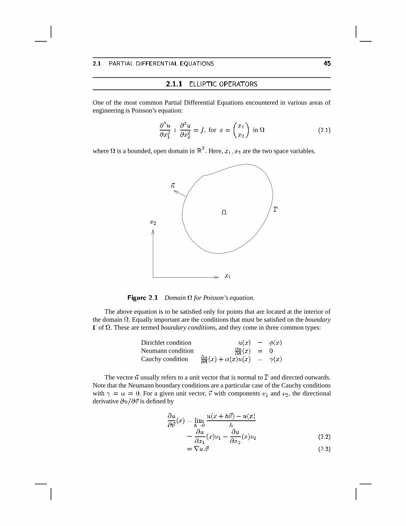
� � � � � ��LK ��Mn^K � � ��^K �� ^K � ��

)�� /�2 � �� One of the most common Partial Differential Equations encountered in various areas ofengineering is Poisson’s equation:� $ 8� � $ � �

� $ 8� � $$ ��y� for �\�� $ � in � � �;J ��

where � is a bounded, open domain in �$. Here, � � �� $ are the two space variables.

�~

� $

� �

� �

, � �� 6T� Domain � for Poisson’s equation.

The above equation is to be satisfied only for points that are located at the interior ofthe domain � . Equally important are the conditions that must be satisfied on the boundary� of � . These are termed boundary conditions, and they come in three common types:

Dirichlet condition 8 *�� + � ��*�� +Neumann condition � �� *� + � %Cauchy condition � �� *�� + � � *� + 8 *�� + � � *� +

The vector�~ usually refers to a unit vector that is normal to � and directed outwards.

Note that the Neumann boundary conditions are a particular case of the Cauchy conditionswith � � �� % . For a given unit vector,

�� with components � � and � $ , the directionalderivative

�8 �� is defined by�

8� �� *� + � � � �� 8 *� � � �� + ! 8 *�� +��8� � � *�� + � � �

�8� �$ *� + � $ � �[J � �

�� 8 � �� [J � �

� � �� n^K � � �� ^K ��^K � � � � �cn �

where � 8 is the gradient of 8 ,

� 8 �� ! � � � �;J � �

and the dot in (2.3) indicates a dot product of two vectors in �$.

In reality, Poisson’s equation is often a limit case of a time-dependent problem. It can,for example, represent the steady-state temperature distribution in a region � when there isa heat source � that is constant with respect to time. The boundary conditions should thenmodel heat loss across the boundary � .

The particular case where � *�� + �&% , i.e., the equation� 8 �=%z�

to which boundary conditions must be added, is called the Laplace equation and its solu-tions are called harmonic functions.

Many problems in physics have boundary conditions of mixed type, e.g., of Dirichlettype in one part of the boundary and of Cauchy type in another. Another observation is thatthe Neumann conditions do not define the solution uniquely. Indeed, if 8 is a solution, thenso is 8M� � for any constant � .

The operator

� �� $�� $ � �

� $�� $$

is called the Laplacean operator and appears in many models of physical and mechanicalphenomena. These models often lead to more general elliptic operators of the form

� ��

��

�� $ � �

�� $ �� R� *k� � + � �;J � �

where the scalar function � depends on the coordinate and may represent some specificparameter of the medium, such as density, porosity, etc. At this point it may be useful torecall some notation which is widely used in physics and mechanics. The � operator canbe considered as a vector consisting of the components �� and �� ! . When applied to ascalar function 8 , this operator is nothing but the gradient operator, since it yields a vectorwith the components � �� and � �� ! as is shown in (2.4). The dot notation allows dot products

of vectors in �$

to be defined. These vectors can include partial differential operators. Forexample, the dot product �R� 8 of � with 8 ��

!�

yields the scalar quantity,�8 ��

�8 $� �$ �

which is called the divergence of the vector function�8 � � � ��

!�. Applying this divergence

operator to 8 � � � , where � is a scalar function, yields the � operator in (2.5). Thedivergence of the vector function

�� is often denoted by div�� or �?� �� . Thus,

div�� R� ��

��

�� $� � $ �

� � � ��K �@K �\n^K � � �� n � � �The closely related operator

� ��

��

�� $ � � $

�� $ �� * ��y� � + � �[J � �

is a further generalization of the Laplacean operator�

in the case where the medium isanisotropic and inhomogeneous. The coefficients � � �6�%$ depend on the space variable � andreflect the position as well as the directional dependence of the material properties, such asporosity in the case of fluid flow or dielectric constants in electrostatics. In fact, the aboveoperator can be viewed as a particular case of � � �R� * � � + , where � is a � � � matrixwhich acts on the two components of � .

)�� *) � ��" �� 6! ! � �� .� �/�2��Many physical problems involve a combination of “diffusion” and “convection” phenom-ena. Such phenomena are modeled by the convection-diffusion equation

�8��

�8� � � �� $

�8� � $ ��R� *k� � + 8M� �

or�8�� 8 ��R� *k� � + 8/� �

the steady-state version of which can be written as

! �?� *w� � + 8Z� �� 8 ��y� � �[J � �Problems of this type are often used as model problems because they represent the simplestform of conservation of mass in fluid mechanics. Note that the vector

�� is sometimes quitelarge, which may cause some difficulties either to the discretization schemes or to theiterative solution techniques.

� � ��

�?|��

The finite difference method is based on local approximations of the partial derivatives ina Partial Differential Equation, which are derived by low order Taylor series expansions.The method is quite simple to define and rather easy to implement. Also, it is particularlyappealing for simple regions, such as rectangles, and when uniform meshes are used. Thematrices that result from these discretizations are often well structured, which means thatthey typically consist of a few nonzero diagonals. Another advantage is that there are anumber of “fast solvers” for constant coefficient problems, which can deliver the solutionin logarithmic time per grid point. This means the total number of operations is of theorder of ~ �� * ~ + where ~ is the total number of discretization points. This section gives

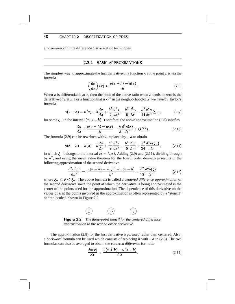
� � �� n^K � � �� ^K ��^K � � � � �cn �

an overview of finite difference discretization techniques.

)��)�� /�*$ � �� The simplest way to approximate the first derivative of a function 8 at the point � is via theformula � ' 8' � � *� + � 8 *� � � + ! 8 *� +� � � �;J �When 8 is differentiable at � , then the limit of the above ratio when � tends to zero is thederivative of 8 at � . For a function that is � � in the neighborhood of � , we have by Taylor’sformula

8 *� � � + � 8 *� + � � ' 8' � � �$�' $ 8' � $ � � �� ' � 8' � � � � �� ' � 8' � � * " + � � �;J � �

for some " in the interval *�x�� + . Therefore, the above approximation (2.8) satisfies' 8' � � 8 *�� + ! 8 *� +� ! � � '

$ 8 *�� +' � $ � � * � $ + � � �;J � � �The formula (2.9) can be rewritten with � replaced by ! � to obtain

8 *��! � + � 8 *� + ! � ' 8' � � �$�' $ 8' � $ ! � �� ' � 8' � � � � �� ' � 8 * � +' � � � � �;J � � �

in which � belongs to the interval *� ! � �� + . Adding (2.9) and (2.11), dividing throughby � $ , and using the mean value theorem for the fourth order derivatives results in thefollowing approximation of the second derivative

' $ 8 *� +' � $ � 8 *� � � + !l� 8 *� + � 8 *� ! � +� $ ! � $�A� ' � 8 * +' � � � � �;J � � �where � � � " . The above formula is called a centered difference approximation ofthe second derivative since the point at which the derivative is being approximated is thecenter of the points used for the approximation. The dependence of this derivative on thevalues of 8 at the points involved in the approximation is often represented by a “stencil”or “molecule,” shown in Figure 2.2.

� !:� �, � �� 6 � The three-point stencil for the centered differenceapproximation to the second order derivative.

The approximation (2.8) for the first derivative is forward rather than centered. Also,a backward formula can be used which consists of replacing � with ! � in (2.8). The twoformulas can also be averaged to obtain the centered difference formula:

' 8 *�� +' � � 8 *�� + ! 8 *�� ! � +� � � � �;J � � �

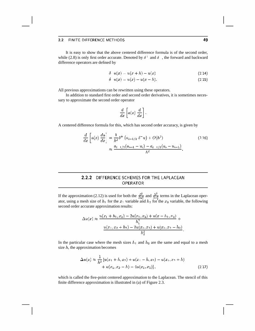
� � � ��K �@K �\n^K � � �� n � � �It is easy to show that the above centered difference formula is of the second order,

while (2.8) is only first order accurate. Denoted by � " and � � , the forward and backwarddifference operators are defined by

� " 8 *�� + � 8 *�� + ! 8 *�� + � �;J � � �� 8 *�� + � 8 *�� + ! 8 *� ! � + � � �;J � � �

All previous approximations can be rewritten using these operators.In addition to standard first order and second order derivatives, it is sometimes neces-

sary to approximate the second order operator

'' � � � *�� + '' � �

A centered difference formula for this, which has second order accuracy, is given by

'' � � � *� + ' 8' � � �

� $ � " � � � � �� $ � � 8 � � � * � $ + � �;J � � ��

� � " �� $ * 8 � " � ! 8 � + !�� $ * 8 � ! 8 � � � +� $ �

)��*)��*) ��! ! �� 1 � � ��$ � ��!#�� 1 � �/��

If the approximation (2.12) is used for both the � !� � ! � and � !� � !! terms in the Laplacean oper-ator, using a mesh size of � � for the � � variable and � $ for the �$ variable, the followingsecond order accurate approximation results:

� 8 *� + � 8 *� � � � � �� $ + !l� 8 *� � �� $ + � 8 *� ! � � �� $ +� $ � �8 *� � ��$ � � $ + !�� 8 *�� $ + � 8 *�� $9! � $ +� $$ �

In the particular case where the mesh sizes � � and � $ are the same and equal to a meshsize � , the approximation becomes

� 8 *� + �

�� $ � 8 *�� $ + � 8 *� � ! � �� $ + � 8 *� � ��$ � � +� 8 *�� $ ! � + ! � 8 *� � ��$ + ! � � �;J � � �

which is called the five-point centered approximation to the Laplacean. The stencil of thisfinite difference approximation is illustrated in (a) of Figure 2.3.

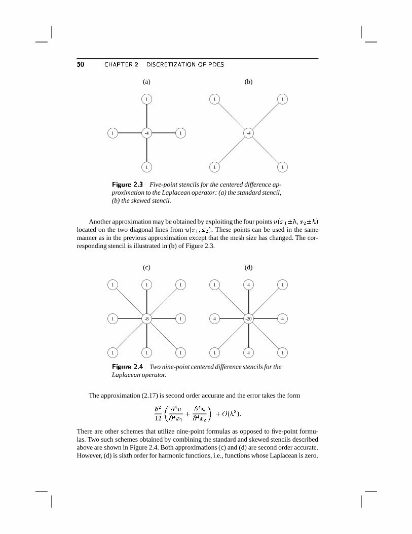
� � �� n^K � � �� ^K ��^K � � � � �cn �(a)

1

1 -4 1

1

(b)

1 1

-4

1 1

, � �� 6 Five-point stencils for the centered difference ap-proximation to the Laplacean operator: (a) the standard stencil,(b) the skewed stencil.

Another approximation may be obtained by exploiting the four points 8 *� � � � �� $ � � +located on the two diagonal lines from 8 *� � �� $ + . These points can be used in the samemanner as in the previous approximation except that the mesh size has changed. The cor-responding stencil is illustrated in (b) of Figure 2.3.

(c)

1 1 1

1 -8 1

1 1 1

(d)

1 4 1

4 -20 4

1 4 1

, � �� 6 � Two nine-point centered difference stencils for theLaplacean operator.

The approximation (2.17) is second order accurate and the error takes the form

� $�A� � � � 8��

�� 8�� $ � � � * � � + �

There are other schemes that utilize nine-point formulas as opposed to five-point formu-las. Two such schemes obtained by combining the standard and skewed stencils describedabove are shown in Figure 2.4. Both approximations (c) and (d) are second order accurate.However, (d) is sixth order for harmonic functions, i.e., functions whose Laplacean is zero.

� � � ��K �@K �\n^K � � �� n � � �)��*)�� ! �*�� ! ! �� 1 � � !#�� $ �

Consider the one-dimensional equation,

! 8 � � *�� + �� *� + for � � * %z�� + � �[J � �8 *�% + � 8 *2� + �=%z� � �;J � � �

The interval [0,1] can be discretized uniformly by taking the ~7� � points

� � �� (�(�=%z��E� ~Z� �where � �� * ~ � � + . Because of the Dirichlet boundary conditions, the values 8 *�� +and 8 *�� " � + are known. At every other point, an approximation 8 � is sought for the exactsolution 8 *� � + .If the centered difference approximation (2.12) is used, then by the equation (2.18)expressed at the point � � , the unknowns 8 � � 8 � � � � 8 � " � satisfy the relation

! 8 � � � � � 8 � ! 8 � " � � � $ � � �in which � � ;

� *� � + . Notice that for �,� � and �,� ~ , the equation will involve 8 � and8 � " � which are known quantities, both equal to zero in this case. Thus, for ~ � � , thelinear system obtained is of the form

� �D� �where

� � �� $

!"""""#� !P�!P� � !P�

!P� � !P�!P� � !P�

!P� � !P�!P� �

& ''''') �

)��*)�� *�� 1��$"� �Consider now the one-dimensional version of the convection-diffusion equation (2.7) inwhich the coefficients � and � are constant, and �\�&% , using Dirichlet boundary conditions,� !`� 8 � � ��<8 � � %z� % � � � � ��

8 *�% + �&%p� 8 * � + � �[� � �;J � � �In this particular case, it is easy to verify that the exact solution to the above equation isgiven by

8 *� + � � ! �� ! � �

where # is the so-called Peclet number defined by # � � � � � . Now consider the approxi-mate solution provided by using the centered difference schemes seen above, for both the

� � �� n^K � � �� ^K ��^K � � � � �cn �

first- and second order derivatives. The equation for unknown number � becomes

� 8 � " � ! 8 � � �� !�� 8 � " � !l� 8 � � 8 � � �� $ �&%p�or, defining �`� # � � � ,

! *_� !�� + 8 � " � � � 8 � ! *2� � � + 8 � � � � %p� � �;J � � �This is a second order homogeneous linear difference equation and the usual way to solveit is to seek a general solution in the form 8 � � � � . Substituting in (2.21), � must satisfy*2�9!�� + � $ !l� �`� *k� � � + � %z�Therefore, � � � � is a root and the second root is � $ � *2� � � + � *_�1!�� + . The generalsolution of the above difference equation is now sought as a linear combination of the twosolutions corresponding to these two roots,

8 � �� $ � � � � � � � �� !�� Because of the boundary condition 8 � � % , it is necessary that

� � ! � . Likewise, theboundary condition 8 � " � �� yields��

� ! : � " � with : ;� � �� !��

Thus, the solution is

8 � � � ! : �� ! : � " � �When � �� # the factor : becomes negative and the above approximations will oscillatearound zero. In contrast, the exact solution is positive and monotone in the range � %p�� ! . Inthis situation the solution is very inaccurate regardless of the arithmetic. In other words,the scheme itself creates the oscillations. To avoid this, a small enough mesh � can betaken to ensure that � � � . The resulting approximation is in much better agreement withthe exact solution. Unfortunately, this condition can limit the mesh size too drastically forlarge values of � .

Note that when � � % , the oscillations disappear since : �� . In fact, a linear algebrainterpretation of the oscillations comes from comparing the tridiagonal matrices obtainedfrom the discretization. Again, for the case ~ � � , the tridiagonal matrix resulting fromdiscretizing the equation (2.7) takes the form

� � �� $

!"""""#

� !P� � �!P� !�� !P� � �!P� !�� !P� � �!P� !�� !P� � �!P� !�� !P� � �!P� !��

& ''''') �

The above matrix is no longer a diagonally dominant M-matrix. Observe that if the back-ward difference formula for the first order derivative is used, we obtain

� 8 � ! 8 � � �� !�� 8 � � � !�� 8 � � 8 � " �� $ �=%z�

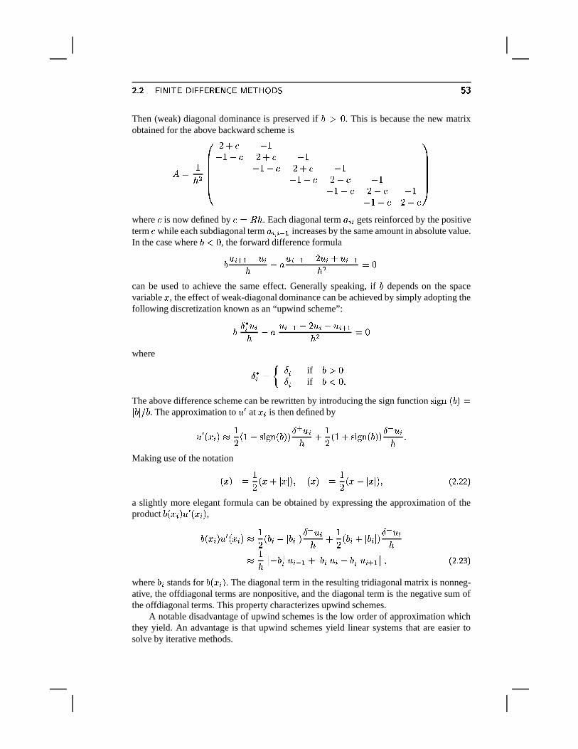
� � � ��K �@K �\n^K � � �� n � �7

Then (weak) diagonal dominance is preserved if � � % . This is because the new matrixobtained for the above backward scheme is

� � �� $

!"""""#� � � !P�!P� !�� !P�

!P� !�� !P�!P� !�� !P�

!P� !�� !P�!P� !��

&(''''')

where � is now defined by �� # � . Each diagonal term � �8� gets reinforced by the positiveterm � while each subdiagonal term � �� increases by the same amount in absolute value.In the case where � � % , the forward difference formula

� 8 � " � ! 8 �� !�� 8 � � � !�� 8 � � 8 � " �� $ �=%can be used to achieve the same effect. Generally speaking, if � depends on the spacevariable � , the effect of weak-diagonal dominance can be achieved by simply adopting thefollowing discretization known as an “upwind scheme”:

� � � 8 �� !�� 8 � � � !�� 8 � � 8 � " �� $ �=%where

� � � � � �� if � � %� "� if � � %z�

The above difference scheme can be rewritten by introducing the sign function � � �� * � + �� . The approximation to 8 � at � � is then defined by

8 � *�� + �

�� *_�9! � � ��* � + + � " 8 ��

� *_� � � � ��* � + + � �-8 �� Making use of the notation*� + " � �

� *� � � � � + � *� + � � �� *��! � � � + � � �;J � � �

a slightly more elegant formula can be obtained by expressing the approximation of theproduct � *� � + 8 � *� � + ,

� *� � + 8 � *� � + �

�� * � � ! � � � � + �

" 8 �� * � � � � � � � + � �-8 ��

�

�� ! � "� 8 � � � � � � � � 8 � �� 8 � " � � � � �;J � � �

where � � stands for � *� � + . The diagonal term in the resulting tridiagonal matrix is nonneg-ative, the offdiagonal terms are nonpositive, and the diagonal term is the negative sum ofthe offdiagonal terms. This property characterizes upwind schemes.

A notable disadvantage of upwind schemes is the low order of approximation whichthey yield. An advantage is that upwind schemes yield linear systems that are easier tosolve by iterative methods.

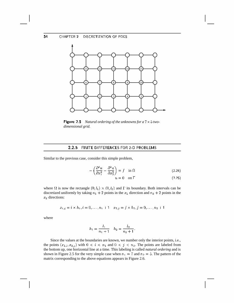
� � �� n^K � � �� ^K ��^K � � � � �cn �

1 2 3 4 5

6 7 8 9 10

11 12 13 14 15

�

�

, � �� 6 � Natural ordering of the unknowns for a �L� � two-dimensional grid.

)��)�� ! �� ! ! �� !#�� $ �Similar to the previous case, consider this simple problem,

! � � $ 8� � $ � �� $ 8� � $$ � �� in � � �;J � � �

8 �=% on � � �;J � � �where � is now the rectangle *�%p� 3 � + � *�%p� 3 $ + and � its boundary. Both intervals can bediscretized uniformly by taking ~ � � � points in the � � direction and ~ $ � � points in the� $ directions:

� � � �(�s� � � � �2��&%p��E� ~ � � � � $ � �� $ �H�}�=%z�� ~ $ � �where

� � � 3 �~ � � � � $:� 3 $

~ $ � � �Since the values at the boundaries are known, we number only the interior points, i.e.,

the points *�� $ � � + with % � � � ~ � and % � � � ~ $ . The points are labeled fromthe bottom up, one horizontal line at a time. This labeling is called natural ordering and isshown in Figure 2.5 for the very simple case when ~ � � � and ~ $ � � . The pattern of thematrix corresponding to the above equations appears in Figure 2.6.

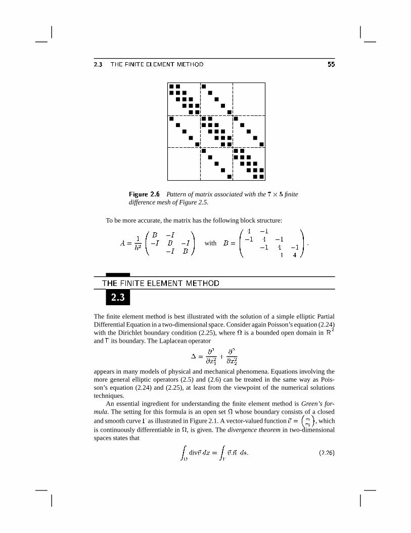
� � � � � ��K �@K � �� 7� � � � �� n � �

, � �� 6 � Pattern of matrix associated with the �Z� � finitedifference mesh of Figure 2.5.

To be more accurate, the matrix has the following block structure:

� � �� $

!# � ! �! � � ! �

! � �&) with � �

!"#� !P�!P� � !P�

!P� � !P�!P� �

&(') �

��

�?|��

The finite element method is best illustrated with the solution of a simple elliptic PartialDifferential Equation in a two-dimensional space. Consider again Poisson’s equation (2.24)with the Dirichlet boundary condition (2.25), where � is a bounded open domain in �

$and � its boundary. The Laplacean operator

� �� $�� $ � �

� $�� $$

appears in many models of physical and mechanical phenomena. Equations involving themore general elliptic operators (2.5) and (2.6) can be treated in the same way as Pois-son’s equation (2.24) and (2.25), at least from the viewpoint of the numerical solutionstechniques.

An essential ingredient for understanding the finite element method is Green’s for-mula. The setting for this formula is an open set � whose boundary consists of a closedand smooth curve � as illustrated in Figure 2.1. A vector-valued function

�� !�

, whichis continuously differentiable in � , is given. The divergence theorem in two-dimensionalspaces states that ��

div�� ' �D� �� ~ ' � � � �;J � � �

� � �� n^K � � �� ^K ��^K � � � � �cn �

The dot in the right-hand side represents a dot product of two vectors in �$. In this case it is

between the vector�� and the unit vector

�~ which is normal to � at the point of considerationand oriented outward. To derive Green’s formula, consider a scalar function � and a vectorfunction

��3� ��

� !�. By standard differentiation,�R� * � �� + ��* � � + � �� R� ��}�

which expresses � � � �� as � � � ��3� ! � �R� �� R� * � �� + � � �;J �� Integrating the above equality over � and using the divergence theorem, we obtain� � � � � �� ' �D��! � �

� �R� �� ' � �� ?� * � �� + ' �

��! � �� R� �� ' � �

� �� b� �~ ' � � � �;J ��

The above equality can be viewed as a generalization of the standard integration by partformula in calculus. Green’s formula results from (2.28) by simply taking a vector

�� whichis itself a gradient of a scalar function 8 , namely,

��3� � 8 ,� � � � � � 8 ' �D� ! �� R� � 8 ' � �

� �� 8 � �~ ' � �

Observe that �R� � 8 � � 8 . Also the function � 8 � �~ is called the normal derivative and isdenoted by

� 8 � �~ ��8� �~ �

With this, we obtain Green’s formula� � � � � � 8 ' �D� ! � �� 8 ' � �

� ��

�8� �~ ' � � � �;J � � �

We now return to the initial problem (2.24-2.25). To solve this problem approximately, itis necessary to (1) take approximations to the unknown function 8 , and (2) translate theequations into a system which can be solved numerically. The options for approximating8 are numerous. However, the primary requirement is that these approximations should bein a (small) finite dimensional space. There are also some additional desirable numericalproperties. For example, it is difficult to approximate high degree polynomials numerically.To extract systems of equations which yield the solution, it is common to use the weakformulation of the problem. Let us define

� * 8 � � +<;�� 8 � � � ' �R� � � � � 8� � �

��

�8� � $�� $ � ' �x�

* �y� � + ; � � � � ' �g�An immediate property of the functional � is that it is bilinear. That means that it is linearwith respect to 8 and � , namely,

� * � � 8 � � � $ 8 $ � � + � � � � * 8 � � � + � � $ � * 8 $ � � + �� $ � � ��* 8 � ( � � � � ( $ � $ + � ( � � * 8 � � � + � ( $ � * 8 � � $ + �� ( � � ( $ � � �

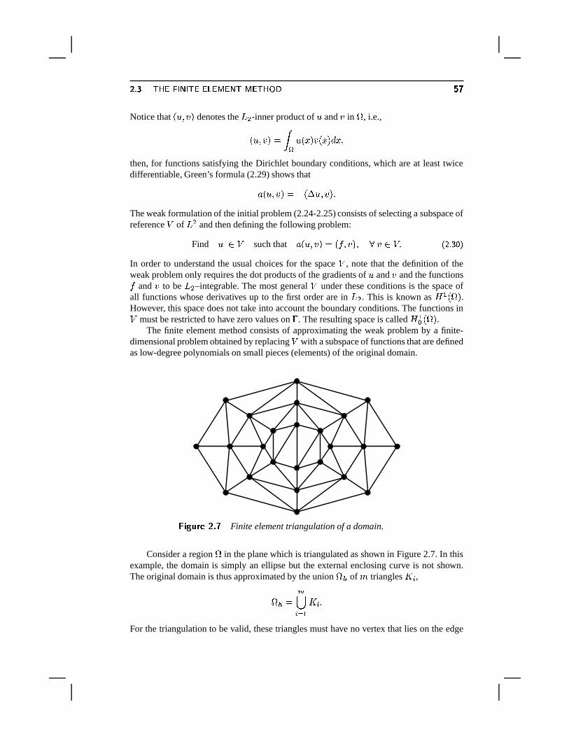
� � � � � ��K �@K � �� 7� � � � �� n � �Notice that * 8 � � + denotes the � $ -inner product of 8 and � in � , i.e.,* 8 � � + � � �

8 *� + � *�� + ' �x�then, for functions satisfying the Dirichlet boundary conditions, which are at least twicedifferentiable, Green’s formula (2.29) shows that

� * 8 � � + � ! * � 8 � � + �The weak formulation of the initial problem (2.24-2.25) consists of selecting a subspace ofreference � of �

$and then defining the following problem:

Find 8 � � such that �* 8 � � + � * �y� � + � � � �� ;J � � �In order to understand the usual choices for the space � , note that the definition of theweak problem only requires the dot products of the gradients of 8 and � and the functions� and � to be � $ –integrable. The most general � under these conditions is the space ofall functions whose derivatives up to the first order are in � $ . This is known as �

� * � + .However, this space does not take into account the boundary conditions. The functions in� must be restricted to have zero values on � . The resulting space is called �� * � + .The finite element method consists of approximating the weak problem by a finite-

dimensional problem obtained by replacing � with a subspace of functions that are definedas low-degree polynomials on small pieces (elements) of the original domain.

, � �� 6 � Finite element triangulation of a domain.

Consider a region � in the plane which is triangulated as shown in Figure 2.7. In thisexample, the domain is simply an ellipse but the external enclosing curve is not shown.The original domain is thus approximated by the union � � of � triangles

� � ,� � � ��

For the triangulation to be valid, these triangles must have no vertex that lies on the edge

� � �� n^K � � �� ^K ��^K � � � � �cn �

of any other triangle. The mesh size � is defined by

� � �� diam * � � +where diam * � + , the diameter of a triangle

�, is the length of its longest side.

Then the finite dimensional space � � is defined as the space of all functions whichare piecewise linear and continuous on the polygonal region � � , and which vanish on theboundary � . More specifically,� � � � � � �� continuous � ��

�� &%z� �� linear �>� � �

Here, �� represents the restriction of the function � to the subset � . If �y�[�H�R� �;��E� ~are the nodes of the triangulation, then a function �y� in � � can be associated with eachnode �z� , so that the family of functions �� ’s satisfies the following conditions:

� � *� � + �=� �0� � � � if � � � � �% if � � � � � � � �;J � � �

These conditions define �d�2�6�@� �[�� ~ uniquely. In addition, the �d� ’s form a basis of thespace � � .

Each function of � � can be expressed as

� *�� + � �� y� *� + �The finite element approximation consists of writing the Galerkin condition (2.30) for func-tions in � � . This defines the approximate problem:

Find 8 � � � such that � * 8 � � + � * �y� � + � � � � � � � � �;J � � �Since 8 is in � � , there are ~ degrees of freedom. By the linearity of � with respect to � , itis only necessary to impose the condition � * 8 � � � + � * �y� � � + for �� ;��E� ~ . This resultsin ~ constraints.

Writing the desired solution 8 in the basis � �d� � as

8 � �� *� +and substituting in (2.32) gives the linear problem

�� F� � � � � � �;J � � �where �x�0�:� � * �y�6� �z� + � � �g� * �y� �y� + �The above equations form a linear system of equations

� �R� � �in which the coefficients of � are the ��0� ’s; those of � are the

� � ’s. In addition, � is aSymmetric Positive Definite matrix. Indeed, it is clear that� � � �y� � �z��' �R� � � � �z� � �y� ' �x�

� � � � � ��K �@K � �� 7� � � � �� n � �which means that � �0� � � �6� . To see that � is positive definite, first note that � * 8 � 8 + � %for any function 8 . If � * �x� � + � % for a function in � � , then it must be true that � �� %almost everywhere in � � . Since � is linear in each triangle and continuous, then it is clearthat it must be constant on all � . Since, in addition, it vanishes on the boundary, then itmust be equal to zero on all of � . The result follows by exploiting the relation

* � u� + �� * �x� � + with �\� �� which is valid for any vector �� .

Another important observation is that the matrix � is also sparse. Indeed, �L�0� isnonzero only when the two basis functions �h� and �z� have common support triangles,or equivalently when the nodes � and � are the vertices of a common triangle. Specifically,for a given node � , the coefficient � �0� will be nonzero only when the node � is one of thenodes of a triangle that is adjacent to node � .

In practice, the matrix is built by summing up the contributions of all triangles byapplying the formula

� * �y�+� �z� + � � � � � * �y�+� �z� +in which the sum is over all the triangles

�and

� � * �y�+� �z� + � �� y� � �u� ' �x�

Note that � � * �y�6� �z� + is zero unless the nodes � and � are both vertices of�

. Thus, a trianglecontributes nonzero values to its three vertices from the above formula. The �M� � matrix

� � �!# � � * ��+� �� + � � * ��+� �u� + � � * �y�+� � � +� � * �z�[� �y� + � � * �z�[� �z� + � � * �z�[� � � +� � * � � � �y� + � � * � � � �z� + � � * � � � � � +

&)associated with the triangle

� *r�<�H�[� � + with vertices �<�=�;� � is called an element stiffnessmatrix. In order to form the matrix � , it is necessary to sum up all the contributions� � * � � � � �0+ to the position � � � of the matrix. This process is called an assembly pro-cess. In the assembly, the matrix is computed as

� � �� ;J � � �

in which ~ � 3 is the number of elements. Each of the matrices � � � � is of the form

� � � � � � � �� /�where � �� is the element matrix for the element

�� as defined above. Also � is an ~\� �

Boolean connectivity matrix which maps the coordinates of the �M� � matrix � � � into thecoordinates of the full matrix � .

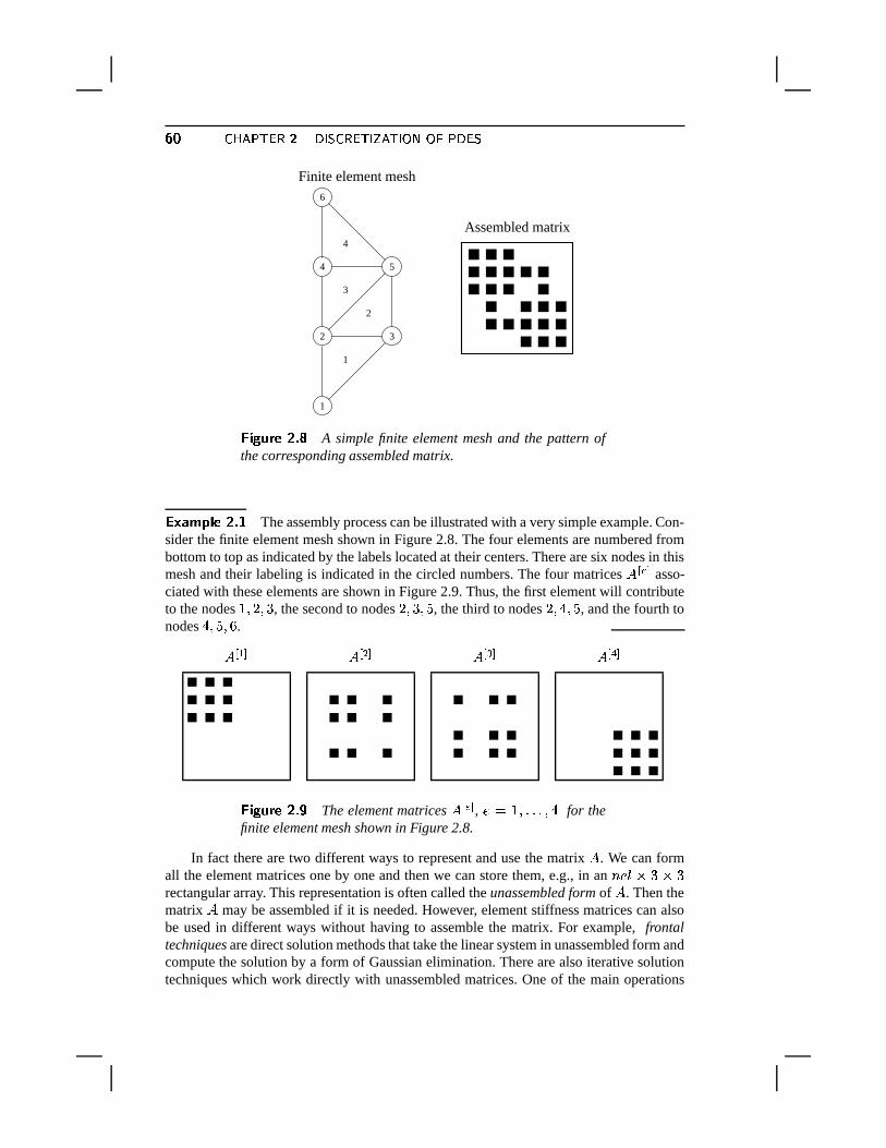
� � �� n^K � � �� ^K ��^K � � � � �cn �Finite element mesh

1

2 3

4 5

6

1

2

3

4

Assembled matrix

, � �� 6 � A simple finite element mesh and the pattern ofthe corresponding assembled matrix.

� �� 6T� The assembly process can be illustrated with a very simple example. Con-sider the finite element mesh shown in Figure 2.8. The four elements are numbered frombottom to top as indicated by the labels located at their centers. There are six nodes in thismesh and their labeling is indicated in the circled numbers. The four matrices � � � � asso-ciated with these elements are shown in Figure 2.9. Thus, the first element will contributeto the nodes �;�+�u� � , the second to nodes �u� � � � , the third to nodes �u� �� , and the fourth tonodes �� .

� � � � � � $ � � � � � � � � �

, � �� 6 � The element matrices � � � � , �?� �[�� for thefinite element mesh shown in Figure 2.8.

In fact there are two different ways to represent and use the matrix � . We can formall the element matrices one by one and then we can store them, e.g., in an ~ � 3j� �D� �rectangular array. This representation is often called the unassembled form of � . Then thematrix � may be assembled if it is needed. However, element stiffness matrices can alsobe used in different ways without having to assemble the matrix. For example, frontaltechniques are direct solution methods that take the linear system in unassembled form andcompute the solution by a form of Gaussian elimination. There are also iterative solutiontechniques which work directly with unassembled matrices. One of the main operations

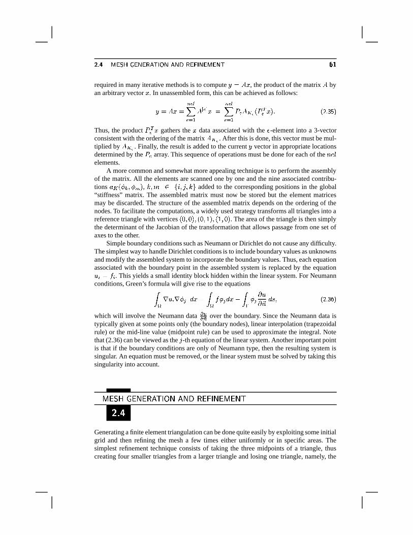
� � � � � � � �� ^K �� @n ��K � 7� �� y�

required in many iterative methods is to compute �R� � � , the product of the matrix � byan arbitrary vector � . In unassembled form, this can be achieved as follows:

�M� � �\� ��

�� * /� � + � � �;J � � �

Thus, the product /� � gathers the � data associated with the � -element into a 3-vectorconsistent with the ordering of the matrix � �� . After this is done, this vector must be mul-tiplied by � �� . Finally, the result is added to the current � vector in appropriate locationsdetermined by the � array. This sequence of operations must be done for each of the ~ � 3elements.

A more common and somewhat more appealing technique is to perform the assemblyof the matrix. All the elements are scanned one by one and the nine associated contribu-tions � � * � � � � � + , � � � � ��<�H�[� � � added to the corresponding positions in the global“stiffness” matrix. The assembled matrix must now be stored but the element matricesmay be discarded. The structure of the assembled matrix depends on the ordering of thenodes. To facilitate the computations, a widely used strategy transforms all triangles into areference triangle with vertices *�%p�#% + � * %z�� + � *_�;�#% + . The area of the triangle is then simplythe determinant of the Jacobian of the transformation that allows passage from one set ofaxes to the other.

Simple boundary conditions such as Neumann or Dirichlet do not cause any difficulty.The simplest way to handle Dirichlet conditions is to include boundary values as unknownsand modify the assembled system to incorporate the boundary values. Thus, each equationassociated with the boundary point in the assembled system is replaced by the equation8 � � � � . This yields a small identity block hidden within the linear system. For Neumannconditions, Green’s formula will give rise to the equations� � � 8 � � �u� ' �R� � � � �z� ' � � � � �u�

�8� �~ ' � � � �;J � � �

which will involve the Neumann data � �� over the boundary. Since the Neumann data istypically given at some points only (the boundary nodes), linear interpolation (trapezoidalrule) or the mid-line value (midpoint rule) can be used to approximate the integral. Notethat (2.36) can be viewed as the � -th equation of the linear system. Another important pointis that if the boundary conditions are only of Neumann type, then the resulting system issingular. An equation must be removed, or the linear system must be solved by taking thissingularity into account.

��

�?|��

Generating a finite element triangulation can be done quite easily by exploiting some initialgrid and then refining the mesh a few times either uniformly or in specific areas. Thesimplest refinement technique consists of taking the three midpoints of a triangle, thuscreating four smaller triangles from a larger triangle and losing one triangle, namely, the

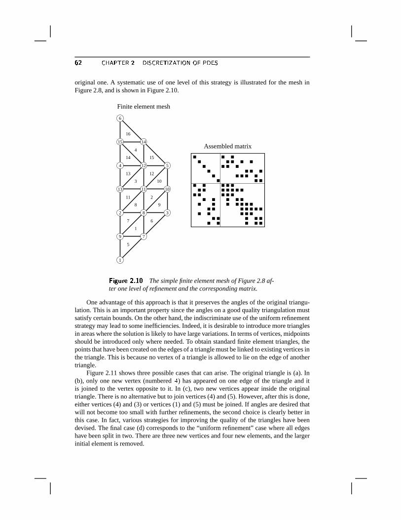
�� n^K � � �� ^K ��^K � � � � �cn �

original one. A systematic use of one level of this strategy is illustrated for the mesh inFigure 2.8, and is shown in Figure 2.10.

Finite element mesh

1

2 3

4 5

6

7

8

9

1011

12

13

1415

1

2

3

4

5

67

8 9

10

11

1213

14 15

16

Assembled matrix

, � �� 6T�� The simple finite element mesh of Figure 2.8 af-ter one level of refinement and the corresponding matrix.

One advantage of this approach is that it preserves the angles of the original triangu-lation. This is an important property since the angles on a good quality triangulation mustsatisfy certain bounds. On the other hand, the indiscriminate use of the uniform refinementstrategy may lead to some inefficiencies. Indeed, it is desirable to introduce more trianglesin areas where the solution is likely to have large variations. In terms of vertices, midpointsshould be introduced only where needed. To obtain standard finite element triangles, thepoints that have been created on the edges of a triangle must be linked to existing vertices inthe triangle. This is because no vertex of a triangle is allowed to lie on the edge of anothertriangle.

Figure 2.11 shows three possible cases that can arise. The original triangle is (a). In(b), only one new vertex (numbered � ) has appeared on one edge of the triangle and itis joined to the vertex opposite to it. In (c), two new vertices appear inside the originaltriangle. There is no alternative but to join vertices (4) and (5). However, after this is done,either vertices (4) and (3) or vertices (1) and (5) must be joined. If angles are desired thatwill not become too small with further refinements, the second choice is clearly better inthis case. In fact, various strategies for improving the quality of the triangles have beendevised. The final case (d) corresponds to the “uniform refinement” case where all edgeshave been split in two. There are three new vertices and four new elements, and the largerinitial element is removed.

� � � ��K �@K �5� � � ?� �� `n �

(a)

1 2

3(b)

1 2

3

4

(c)

1 2

3

4

5

(d)

1 2

3

4

56

, � �� 6T�z� Original triangle (a) and three possible refine-ment scenarios.

� � �� ?|��

The finite volume method is geared toward the solution of conservation laws of the form:�8�� R� �� ;J ��

In the above equation,�� * 8 � � + is a certain vector function of 8 and time, possibly nonlinear.

This is called the “flux vector.” The source term � is a function of space and time. We nowapply the principle used in the weak formulation, described before. Multiply both sides bya test function � , and take the integral� �

�

�8��' � �

� �� R� �� ' �D� � �

� � ' �x�Then integrate by part using formula (2.28) for the second term on the left-hand side toobtain � �

�

�8��' � ! � � � �>� �� ' � �

� �� ~ ' � � � �

� � ' �x�Consider now a control volume consisting, for example, of an elementary triangle

� � inthe two-dimensional case, such as those used in the finite element method. Take for � afunction �`� whose value is one on the triangle and zero elsewhere. The second term in the

� � �� n^K � � �� ^K ��^K � � � � �cn �

above equation vanishes and the following relation results:�� 4

�8��' � �

��4�� ~ ' � � �

� 4 �' �g� � �;J ��

The above relation is at the basis of the finite volume approximation. To go a little further,the assumptions will be simplified slightly by taking a vector function

��that is linear with

respect to 8 . Specifically, assume �� ( � 8( $ 8 � ;

�( 8 �Note that, in this case, the term �R� ��

in (2.37) becomes�� * 8 + � �( � � 8 . In addition, the

right-hand side and the first term in the left-hand side of (2.38) can be approximated asfollows: �

� 4

�8��' � �

�8 ��

� 4 �' � � ��

Here,� � � � represents the volume

�of

� � , and � � is some average value of � in the cell� � .

These are crude approximations but they serve the purpose of illustrating the scheme.The finite volume equation (2.38) yields�

8 �� ( � � � 4 8 �~ ' � �� ;J � � �

The contour integral � �4 8�~ ' �

is the sum of the integrals over all edges of the control volume. Let the value of 8 on eachedge � be approximated by some “average” 38 � . In addition, � � denotes the length of eachedge and a common notation is �� ~ � �Then the contour integral is approximated by�( � � � 4 8 �~ ' � �

��38 � �( � �~ � � � � �

��38 � �( � �� ;J � � �

The situation in the case where the control volume is a simple triangle is depicted in Figure2.12. The unknowns are the approximations 8 � of the function 8 associated with each cell.These can be viewed as approximations of 8 at the centers of gravity of each cell � . Thistype of model is called cell-centered finite volume approximations. Other techniques basedon using approximations on the vertices of the cells are known as cell-vertex finite volumetechniques.

�� !��#"��$��%�'&��($�!��)*�+)*&$�')%,

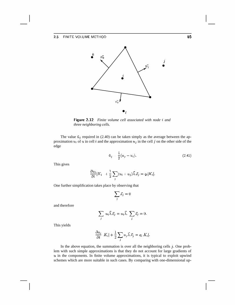
� � � ��K �@K �5� � � ?� �� `n � �

�

�~ �

��~ �

�

�~ ��

��

3, � �� 6T� � Finite volume cell associated with node � andthree neighboring cells.

The value 38 � required in (2.40) can be taken simply as the average between the ap-proximation 8 � of 8 in cell � and the approximation 8 � in the cell � on the other side of theedge

38 �:� �� * 8 � � 8 � + � � �;J � ��

This gives �8 ��

� � � * 8 � � 8 � + �( � ��

One further simplification takes place by observing that�� %

and therefore �� 8 � �( � �� 8 � �( � � � �� %p�

This yields �8 ��

� � � 8 � �( � �� :��

In the above equation, the summation is over all the neighboring cells � . One prob-lem with such simple approximations is that they do not account for large gradients of8 in the components. In finite volume approximations, it is typical to exploit upwindschemes which are more suitable in such cases. By comparing with one-dimensional up-

� � �� n^K � � �� ^K ��^K � � � � �cn �

wind schemes, it can be easily seen that the suitable modification to (2.41) is as follows:38 �`� �� * 8 � � 8 � + ! �

� sign � �( � �� * 8 � ! 8 � + � � �;J � � �This gives

�8 �� ( � ��

� * 8 � � 8 � + ! �� sign * �( � �� + * 8 �9! 8 � + � ��

Now write�8 ��

� * 8 � � 8 � + �( � �� ! �� ( � �� * 8 � ! 8 � + � ��

8 �� 8 � * �( � �� + " � 8 � * �( � �� + � � ��

where * � + �

;

��

��

� �The equation for cell � takes the form

�8 �� 8 � � � � � �0� 8 � ��

where � � � � � * �( � �� + " � %z� � �;J � � �� F� � * �( � �� + � � %z� � �;J � � �

Thus, the diagonal elements of the matrix are nonnegative, while its offdiagonal elementsare nonpositive. In addition, the row-sum of the elements, i.e., the sum of all elements inthe same row, is equal to zero. This is because� � � � � � �F� � � � * �( � �� + " � � � * �( � �� + � � � � �( � �� ( � � � �� %z�The matrices obtained have the same desirable property of weak diagonal dominance seenin the one-dimensional case. A disadvantage of upwind schemes, whether in the context ofirregular grids or in one-dimensional equations, is the loss of accuracy due to the low orderof the schemes.

� � � � � � ��

1 Derive Forward Difference formulas similar to (2.8), i.e., involving ' ?��@BD��' ?�� * BD��' ?�� * BD� #9#9# , which are of second and third order. Write down the discretization errors explicitly.

� �� gK � � � �@n � � � � � �2 Derive a Centered Difference formula for the first derivative, similar to (2.13), which is at least

of third order.

3 Show that the Upwind Difference scheme described in 2.2.4, when % and��

are constant, is stablefor the model problem (2.7).

4 Develop the two nine-point formulas illustrated in Figure 2.4. Find the corresponding discretiza-tion errors. [Hint: Combine 0& of the five-point formula (2.17) plus

#& of the same formula basedon the diagonal stencil � ?�� 'BD�9?�� *-��!� * B,�/?�� *1�� * BD� ?�� *-��!� * BD�9?�� *-�� * B��to get one formula. Use the reverse combination

#& , 0& to get the other formula.]

5 Consider a (two-dimensional) rectangular mesh which is discretized as in the finite differenceapproximation. Show that the finite volume approximation to

�� # � ' yields the same matrix as anupwind scheme applied to the same problem. What would be the mesh of the equivalent upwindfinite difference approximation?

6 Show that the right-hand side of equation (2.16) can also be written as�* #�� . � %� - �

!� - '�#

7 Show that the formula (2.16) is indeed second order accurate for functions that are in $� .8 Show that the functions � � ’s defined by (2.31) form a basis of ?� .

9 Develop the equivalent of Green’s formula for the elliptic operator � defined in (2.6).

10 Write a short FORTRAN or C program to perform a matrix-by-vector product when the matrixis stored in unassembled form.

11 Consider the finite element mesh of Example 2.1. Compare the number of operations required toperform a matrix-by-vector product when the matrix is in assembled and in unassembled form.Compare also the storage required in each case. For a general finite element matrix, what canthe ratio be between the two in the worst case (consider only linear approximations on triangularelements) for arithmetic? Express the number of operations in terms of the number of nodes andedges of the mesh. You may make the assumption that the maximum number of elements thatare adjacent to a given node is � (e.g., � � �

).

12 Let � be a polygon in� #

with � edges, and let�� + � � + � + , for 2 � � � #F#9# �� , where � + is the

length of the 2 -th edge and� + is the unit outward normal at the 2 -th edge. Use the divergence

theorem to prove that��+�� 0

�� + �� .

NOTES AND REFERENCES. The material in this chapter is based on several sources. For a basicdescription of the finite element method, the book by C. Johnson is a good reference [128]. Axelssonand Barker [16] gives a treatment which includes various solution techniques emphasizing iterativetechniques. For finite difference and finite volume methods, we recommend C. Hirsch [121], whichalso gives a good description of the equations and solution methods for fluid flow problems.

� � � � � � �

�

� � � � � � � � � ��

�h�MW!$6�%��&T�0B�$<Wl�0-R"+��$G �&8$6*�� .[CE�/��) #"H$�&we@�="%�!-�W!��&8W�W[� �H��&8$6"2� m+�E"_� .;-E�>.�4��;��&0"2� �!9n(� op$�&q$�-#"2� �!9�[aYC��#"2� .[-E�@"rV! �� <�!9 9 VP9 $<��WN"H.M9 ��&I'�$ �)-�W ��(20 �� Q5�E"6&i� �<$+�<J ��+ ��&I�%$Q5�#"+&T� UL� �yW!$2fp-�$+W�e#�H.;Q5$61L��E"p*��E';C�$�9 V<eE��y� Q5�#"+&T� U(15�� j��E��*�$�&0V�4i$21 -E.[-Em<$�&I.$�9 $�Q5$�-#"H�+J �dC#"+e��0-Z4T��2"<e@�GQ5�E"6&T� UD�<�)- B�$}"%$�&wQ5$<WG�+ ��&I�%$M1L��$�-�$6*�$�&j�+ �$<�E� �!9"H$<��!-�� aYC�$6�j�<�!-ZB�$}C#"2�09 � m<$<W>"H.b"%�!]+$��W�*��!-#"%�E'A$�.�4@"6��$b9 ��&I'A$b-!C!Q:B�$�&g.�4(m<$�&I.$�9 $�Q5$�-#"H�c�)-�Wj"6��$E�0&z9 .)�<�#"2� .[-E�<J �^��$6�%$��+ ��&I�%$jQ5�E"6&i� U5"H$<��!-�� aYC�$6�xB�$+')�0-�1�� "6��"+��$� W!$<�b"6��E"5"+��$Pm<$�&I.?$�9 $�Qj$�-#"H�N-�$<$<WG-E.�"PB�$N�="=.)&8$<W�J�� -�$N.�4L"6��$M]+$2V7� �=�+C�$+�,� �"=.,W!$2fp-�$LW!�#"%� �="+&rC��6"6C!&8$+�x4q.)&z"6��$+�%$:Q5�#"+&T� �<$6�x"+��#"x��&8$L1g$�9 9��+C�� "H$<W:4q.!&y$��N�E� $�-#"�FQ: !9 $�Q5$�-#"%�#"2� .[-,.�4@�="H�)-�W!��&8W/�=.;9 C#"_� .;-MQ5$6"6�E.)WA�<ez15��$6"6��$�&xW[�0&8$<�6"5.!&�� "%$�&8�#"2� *�$�J�� ! #"%$�&�'!� *�$+�,�)-/.�*�$�&0*�� $613.�45�+ ��&I�%$7Qj�#"+&T� �+$+�<ey"6��$E�0&t �&8.[ A$�&I"_� $+�<ec"6��$E�0&&8$� �&8$+�%$�-#"H�E"_� .;-E�<e[�!-�W,"+��$tW!�#"%�`�="6&wC��2"+C!&8$+�tCE�%$<W,"=.N�="=.)&8$t"+��$�Q�J

� ��

�7|E{

The natural idea to take advantage of the zeros of a matrix and their location was initiatedby engineers in various disciplines. In the simplest case involving banded matrices, specialtechniques are straightforward to develop. Electrical engineers dealing with electrical net-works in the 1960s were the first to exploit sparsity to solve general sparse linear systemsfor matrices with irregular structure. The main issue, and the first addressed by sparse ma-trix technology, was to devise direct solution methods for linear systems. These had to beeconomical, both in terms of storage and computational effort. Sparse direct solvers canhandle very large problems that cannot be tackled by the usual “dense” solvers.

� �

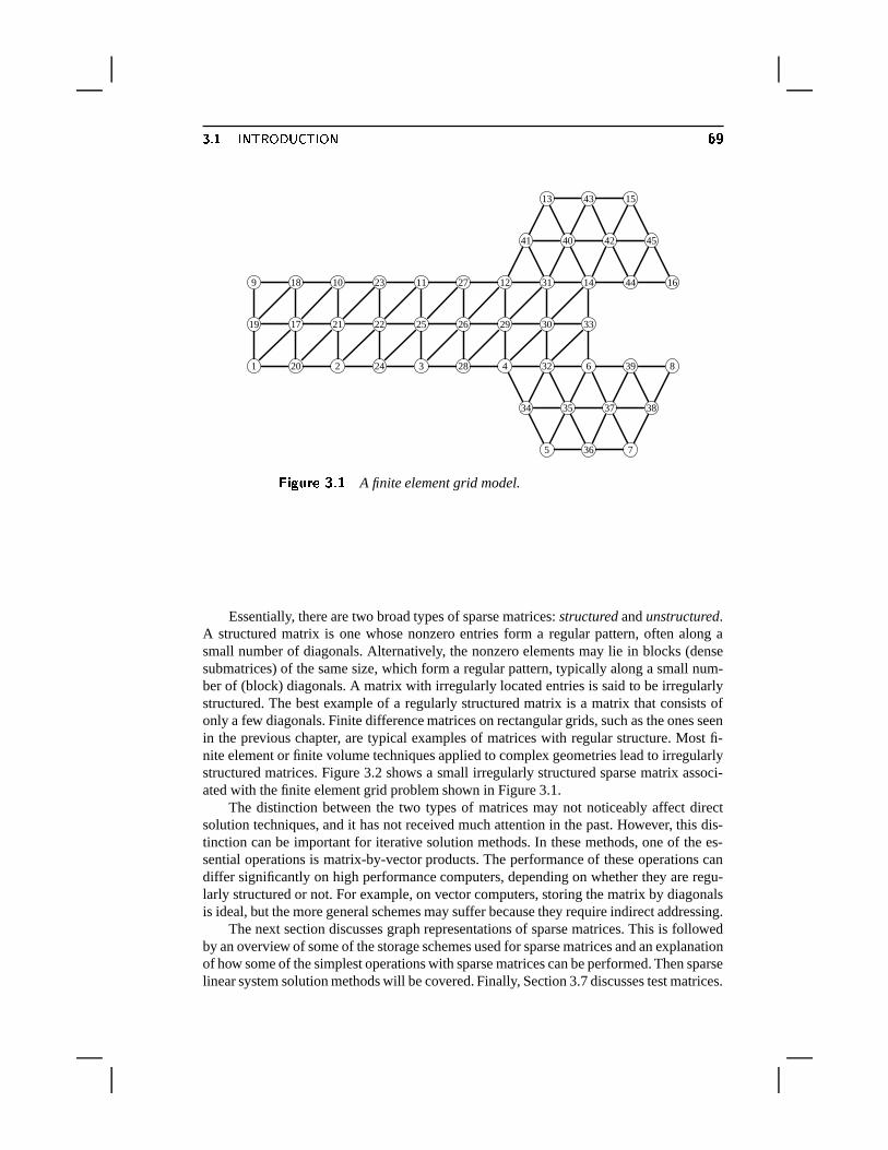
�� K � � � � n� � �^K � � � �

1 2 3 4

5

6

7

8

9 10 11 12

13

14

15

16

17

18

19

20

21 22

23

24

25 26

27

28

29 30

31

32

33

34 35

36

37 38

39

4041 42

43

44

45

, � �� 6T� A finite element grid model.

Essentially, there are two broad types of sparse matrices: structured and unstructured.A structured matrix is one whose nonzero entries form a regular pattern, often along asmall number of diagonals. Alternatively, the nonzero elements may lie in blocks (densesubmatrices) of the same size, which form a regular pattern, typically along a small num-ber of (block) diagonals. A matrix with irregularly located entries is said to be irregularlystructured. The best example of a regularly structured matrix is a matrix that consists ofonly a few diagonals. Finite difference matrices on rectangular grids, such as the ones seenin the previous chapter, are typical examples of matrices with regular structure. Most fi-nite element or finite volume techniques applied to complex geometries lead to irregularlystructured matrices. Figure 3.2 shows a small irregularly structured sparse matrix associ-ated with the finite element grid problem shown in Figure 3.1.

The distinction between the two types of matrices may not noticeably affect directsolution techniques, and it has not received much attention in the past. However, this dis-tinction can be important for iterative solution methods. In these methods, one of the es-sential operations is matrix-by-vector products. The performance of these operations candiffer significantly on high performance computers, depending on whether they are regu-larly structured or not. For example, on vector computers, storing the matrix by diagonalsis ideal, but the more general schemes may suffer because they require indirect addressing.

The next section discusses graph representations of sparse matrices. This is followedby an overview of some of the storage schemes used for sparse matrices and an explanationof how some of the simplest operations with sparse matrices can be performed. Then sparselinear system solution methods will be covered. Finally, Section 3.7 discusses test matrices.

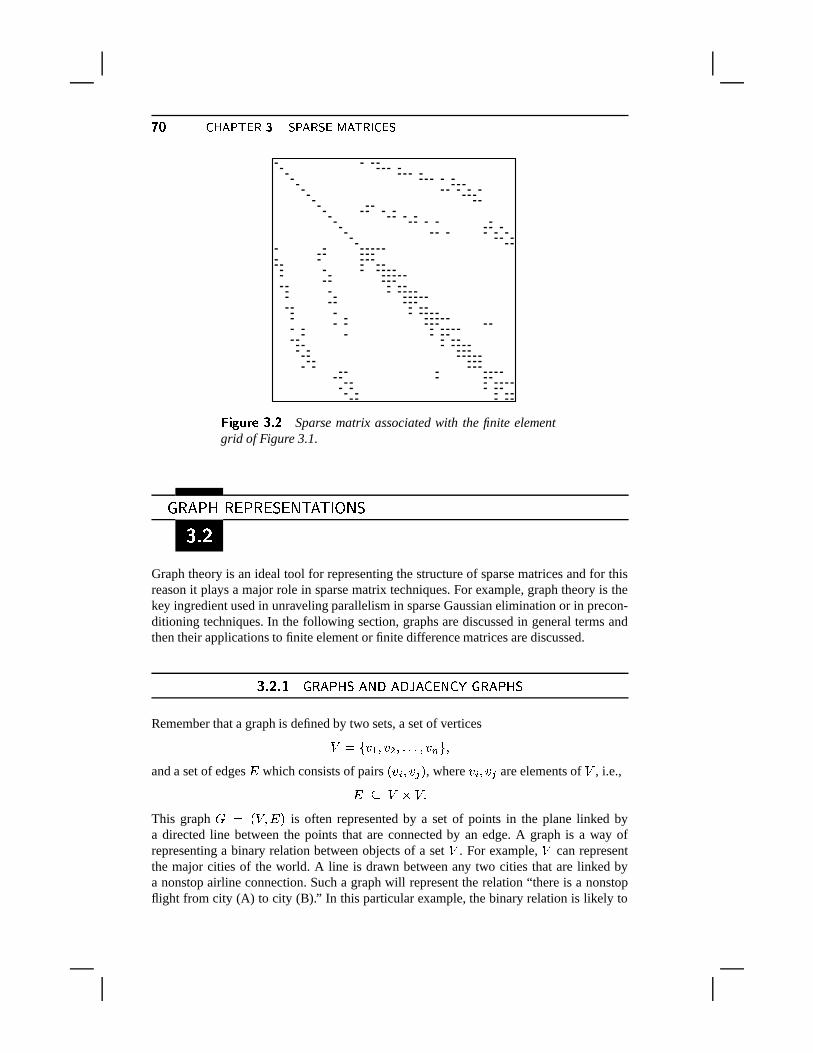
� � �� dK � �

, � �� 6 � Sparse matrix associated with the finite elementgrid of Figure 3.1.

� � � � � � � � � �� 7|��

Graph theory is an ideal tool for representing the structure of sparse matrices and for thisreason it plays a major role in sparse matrix techniques. For example, graph theory is thekey ingredient used in unraveling parallelism in sparse Gaussian elimination or in precon-ditioning techniques. In the following section, graphs are discussed in general terms andthen their applications to finite element or finite difference matrices are discussed.

��)�� /�� /�+ �� 1 �� Remember that a graph is defined by two sets, a set of vertices� � � � � � � $ �� and a set of edges � which consists of pairs * � � � � � + , where � � � � � are elements of � , i.e.,

�� This graph � � * � � � + is often represented by a set of points in the plane linked bya directed line between the points that are connected by an edge. A graph is a way ofrepresenting a binary relation between objects of a set � . For example, � can representthe major cities of the world. A line is drawn between any two cities that are linked bya nonstop airline connection. Such a graph will represent the relation “there is a nonstopflight from city (A) to city (B).” In this particular example, the binary relation is likely to

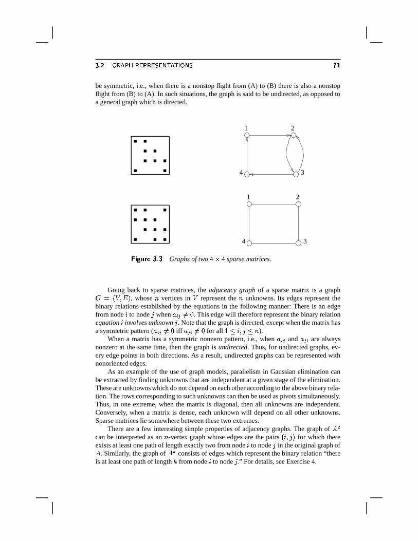
�� ^K � � � � �be symmetric, i.e., when there is a nonstop flight from (A) to (B) there is also a nonstopflight from (B) to (A). In such situations, the graph is said to be undirected, as opposed toa general graph which is directed.

1 2

4 3

1 2

4 3

, � �� 6 Graphs of two � � � sparse matrices.

Going back to sparse matrices, the adjacency graph of a sparse matrix is a graph� � * � � � + , whose ~ vertices in � represent the ~ unknowns. Its edges represent thebinary relations established by the equations in the following manner: There is an edgefrom node � to node � when � �F� �=% . This edge will therefore represent the binary relationequation � involves unknown � . Note that the graph is directed, except when the matrix hasa symmetric pattern ( � �0� �&% iff � �6� �&% for all � � �<�=� � ~ ).

When a matrix has a symmetric nonzero pattern, i.e., when �p�0� and �[�6� are alwaysnonzero at the same time, then the graph is undirected. Thus, for undirected graphs, ev-ery edge points in both directions. As a result, undirected graphs can be represented withnonoriented edges.

As an example of the use of graph models, parallelism in Gaussian elimination canbe extracted by finding unknowns that are independent at a given stage of the elimination.These are unknowns which do not depend on each other according to the above binary rela-tion. The rows corresponding to such unknowns can then be used as pivots simultaneously.Thus, in one extreme, when the matrix is diagonal, then all unknowns are independent.Conversely, when a matrix is dense, each unknown will depend on all other unknowns.Sparse matrices lie somewhere between these two extremes.

There are a few interesting simple properties of adjacency graphs. The graph of � $can be interpreted as an ~ -vertex graph whose edges are the pairs *r�<�H� + for which thereexists at least one path of length exactly two from node � to node � in the original graph of� . Similarly, the graph of � � consists of edges which represent the binary relation “thereis at least one path of length � from node � to node � .” For details, see Exercise 4.

� � �� dK � ��)��*) �� ! �&$ � �� 2 1� �

For Partial Differential Equations involving only one physical unknown per mesh point, theadjacency graph of the matrix arising from the discretization is often the graph representedby the mesh itself. However, it is common to have several unknowns per mesh point. Forexample, the equations modeling fluid flow may involve the two velocity components ofthe fluid (in two dimensions) as well as energy and momentum at each mesh point. Insuch situations, there are two choices when labeling the unknowns. They can be labeledcontiguously at each mesh point. Thus, for the example just mentioned, we can label allfour variables (two velocities followed by momentum and then pressure) at a given meshpoint as 8 * � + , �� , 8 * �p� � + . Alternatively, all unknowns associated with one type of variablecan be labeled first (e.g., first velocity components), followed by those associated with thesecond type of variables (e.g., second velocity components), etc. In either case, it is clearthat there is redundant information in the graph of the adjacency matrix. The quotient graphcorresponding to the physical mesh can be used instead. This results in substantial savingsin storage and computation. In the fluid flow example mentioned above, the storage canbe reduced by a factor of almost 16 for the integer arrays needed to represent the graph.This is because the number of edges has been reduced by this much, while the number ofvertices, which is usually much smaller, remains the same.

� � � � � � � � � � �� 7|��

Permuting the rows or the columns, or both the rows and columns, of a sparse matrix is acommon operation. In fact, reordering rows and columns is one of the most important in-gredients used in parallel implementations of both direct and iterative solution techniques.This section introduces the ideas related to these reordering techniques and their relationsto the adjacency graphs of the matrices. Recall the notation introduced in Chapter 1 thatthe � -th column of a matrix is denoted by � � and the � -th row by � � .

�� 2 � ��1 � � �We begin with a definition and new notation.

+ � , .�01.q�2.43 0 6T� Let � be a matrix and � � �� 2� $!��2� � � a permutation of the set�;�;�+�u��#� ~ � . Then the matrices

�� :� �� A� � � �� A� � � ��

are called row � -permutation and column � -permutation of � , respectively.

�� ^K � � �� @n �� dn �dK �� $It is well known that any permutation of the set �Y�[�<�u��#� ~ � results from at most ~ inter-changes, i.e., elementary permutations in which only two entries have been interchanged.An interchange matrix is the identity matrix with two of its rows interchanged. Denote by� �0� such matrices, with � and � being the numbers of the interchanged rows. Note thatin order to interchange rows � and � of a matrix � , we only need to premultiply it by thematrix � �0� . Let � � �� 2� $ ��2� � � be an arbitrary permutation. This permutation is theproduct of a sequence of ~ consecutive interchanges : *w� � �=� � + � � � �;��E� ~ . Then therows of a matrix can be permuted by interchanging rows � � �H� � , then rows � $ �H� $ of theresulting matrix, etc., and finally by interchanging � � �=� � of the resulting matrix. Each ofthese operations can be achieved by a premultiplication by � � � � � � . The same observationcan be made regarding the columns of a matrix: In order to interchange columns � and � of amatrix, postmultiply it by � �F� . The following proposition follows from these observations.

�5�<3/�<32>?.8�1.4350 6T� Let � be a permutation resulting from the product of the inter-changes : *r� � �=� � + , � ��[�� ~ . Then,

� � � � � � � � � � � � � � �where � � � � � � � � � � � � �

� ��

�� [J �� "� �

!� �!�� [J � �

Products of interchange matrices are called permutation matrices. Clearly, a permutationmatrix is nothing but the identity matrix with its rows (or columns) permuted.

Observe that � $�� , i.e., the square of an interchange matrix is the identity, or

equivalently, the inverse of an interchange matrix is equal to itself, a property which isintuitively clear. It is easy to see that the matrices (3.1) and (3.2) satisfy ��

� ��

�� N� � � � � � �"� �!� �!��

which shows that the two matrices � � and � are nonsingular and that they are the inverseof one another. In other words, permuting the rows and the columns of a matrix, usingthe same permutation, actually performs a similarity transformation. Another importantconsequence arises because the products involved in the definitions (3.1) and (3.2) of �and � � occur in reverse order. Since each of the elementary matrices � � � � � � is symmetric,the matrix � � is the transpose of � . Therefore,

� � � /� � � �� Since the inverse of the matrix � is its own transpose, permutation matrices are unitary.

Another way of deriving the above relationships is to express the permutation matrices � and /� in terms of the identity matrix, whose columns or rows are permuted. It caneasily be seen (See Exercise 3) that � � �

�� !� /� � � �

��

It is then possible to verify directly that

� � � � ��

�� /� �

� � �� dK � �

It is important to interpret permutation operations for the linear systems to be solved.When the rows of a matrix are permuted, the order in which the equations are written ischanged. On the other hand, when the columns are permuted, the unknowns are in effectrelabeled, or reordered.

� �� 6T� Consider, for example, the linear system � �D� � where

� �!"#� � � % � �� %% �%$-$ �%$ � � $ �� $ � �� %% � � $ % � � �

&(')

and � ��;�;� � �<�u� � � , then the (column-) permuted linear system is!"#� � � � � � % %% � $ � � $ $ � $ �� $ %% % � � $ � � �

&(')!"#� �� $� �

&(') �

!"# �� $� �� &(') �

Note that only the unknowns have been permuted, not the equations, and in particular, theright-hand side has not changed.

In the above example, only the columns of � have been permuted. Such one-sidedpermutations are not as common as two-sided permutations in sparse matrix techniques.In reality, this is often related to the fact that the diagonal elements in linear systems playa distinct and important role. For instance, diagonal elements are typically large in PDEapplications and it may be desirable to preserve this important property in the permutedmatrix. In order to do so, it is typical to apply the same permutation to both the columnsand the rows of � . Such operations are called symmetric permutations, and if denoted by� � � � , then the result of such symmetric permutations satisfies the relation

�� /� � � �The interpretation of the symmetric permutation is quite simple. The resulting matrix cor-responds to renaming, or relabeling, or reordering the unknowns and then reordering theequations in the same manner.

� �� 6 � For the previous example, if the rows are permuted with the same permu-tation as the columns, the linear system obtained is!"

#� � � � � � % %� �� $ %% �%$ � �%$ $ �%$ �% % � � $ � � �

&(')!"#� �� $� �

&(') �

!"# �� $� �&(') �

Observe that the diagonal elements are now diagonal elements from the original matrix,placed in a different order on the main diagonal.

�� ^K � � �� @n �� dn �dK �� *) �� /�2�� 0� �� /�+ �� 1 ��

From the point of view of graph theory, another important interpretation of a symmetricpermutation is that it is equivalent to relabeling the vertices of the graph without alteringthe edges. Indeed, let *r�<�=� + be an edge in the adjacency graph of the original matrix �and let � � be the permuted matrix. Then � ��F� � �

� � � � � � � � � and a result *r�<�=� + is an edgein the adjacency graph of the permuted matrix � � , if and only if * � *w� + � � *q� +-+ is an edgein the graph of the original matrix � . Thus, the graph of the permuted matrix has notchanged; rather, the labeling of the vertices has. In contrast, nonsymmetric permutationsdo not preserve the graph. In fact, they can transform an indirected graph into a directedone. Symmetric permutations may have a tremendous impact on the structure of the matrixeven though the general graph of the adjacency matrix is identical.

� �� 6 Consider the matrix illustrated in Figure 3.4 together with its adjacencygraph. Such matrices are sometimes called “arrow” matrices because of their shape, but itwould probably be more accurate to term them “star” matrices because of the structure oftheir graphs.

If the equations are reordered using the permutation �p� �z��#�� , the matrix and graphshown in Figure 3.5 are obtained. Although the difference between the two graphs mayseem slight, the matrices have a completely different structure, which may have a signif-icant impact on the algorithms. As an example, if Gaussian elimination is used on thereordered matrix, no fill-in will occur, i.e., the L and U parts of the LU factorization willhave the same structure as the lower and upper parts of � , respectively. On the other hand,Gaussian elimination on the original matrix results in disastrous fill-ins. Specifically, theL and U parts of the LU factorization are now dense matrices after the first step of Gaus-sian elimination. With direct sparse matrix techniques, it is important to find permutationsof the matrix that will have the effect of reducing fill-ins during the Gaussian eliminationprocess.

To conclude this section, it should be mentioned that two-sided nonsymmetric permu-tations may also arise in practice. However, they are more common in the context of directmethods.

�� $ $ �� *�� The type of reordering, or permutations, used in applications depends on whether a director an iterative method is being considered. The following is a sample of such reorderingswhich are more useful for iterative methods.

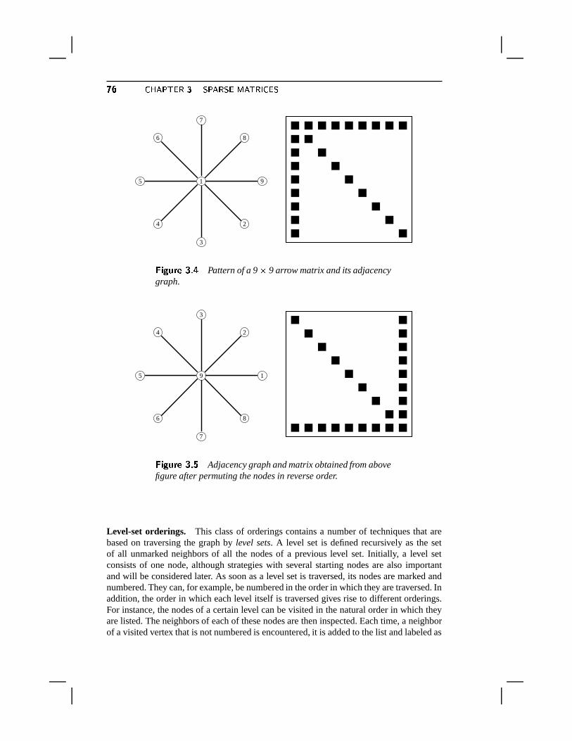
� � �� dK � �

1

2

3

4

5

6

7

8

9

, � �� 6 � Pattern of a 9 � 9 arrow matrix and its adjacencygraph.

1

2

3

4

5

6

7

8

9

, � �� 6 � Adjacency graph and matrix obtained from abovefigure after permuting the nodes in reverse order.

Level-set orderings. This class of orderings contains a number of techniques that arebased on traversing the graph by level sets. A level set is defined recursively as the setof all unmarked neighbors of all the nodes of a previous level set. Initially, a level setconsists of one node, although strategies with several starting nodes are also importantand will be considered later. As soon as a level set is traversed, its nodes are marked andnumbered. They can, for example, be numbered in the order in which they are traversed. Inaddition, the order in which each level itself is traversed gives rise to different orderings.For instance, the nodes of a certain level can be visited in the natural order in which theyare listed. The neighbors of each of these nodes are then inspected. Each time, a neighborof a visited vertex that is not numbered is encountered, it is added to the list and labeled as

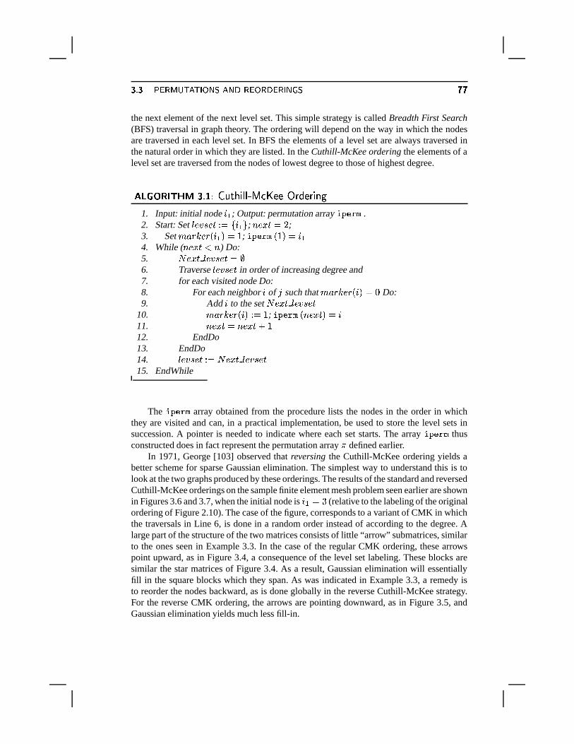
�� ^K � � �� @n �� dn �dK �� the next element of the next level set. This simple strategy is called Breadth First Search(BFS) traversal in graph theory. The ordering will depend on the way in which the nodesare traversed in each level set. In BFS the elements of a level set are always traversed inthe natural order in which they are listed. In the Cuthill-McKee ordering the elements of alevel set are traversed from the nodes of lowest degree to those of highest degree.

�� 3/� .q�P�� 6T� � �� '� �* * �$� ��*� � ��1. Input: initial node � � ; Output: permutation array

��.

2. Start: Set 3 � � � � � � �� ; ~ � � � �3� ;3. Set � � � � � � *r� � + �O� ; �� *_� + �s� �4. While ( ~ � � � � ~ ) Do:5. � � � � 3 � � � � � � �6. Traverse 3 � � � � � in order of increasing degree and7. for each visited node Do:8. For each neighbor � of � such that � � � � � � *w� + � % Do:9. Add � to the set � � � � 3 � � � � �

10. � � � � � � *r� + �� ; �� * ~ � � � + �s�11. ~ � � � � ~ � � � � �12. EndDo13. EndDo14. 3 � � � � � � � � � � 3 � � � � �15. EndWhile

The��

array obtained from the procedure lists the nodes in the order in whichthey are visited and can, in a practical implementation, be used to store the level sets insuccession. A pointer is needed to indicate where each set starts. The array

��thus

constructed does in fact represent the permutation array � defined earlier.In 1971, George [103] observed that reversing the Cuthill-McKee ordering yields a

better scheme for sparse Gaussian elimination. The simplest way to understand this is tolook at the two graphs produced by these orderings. The results of the standard and reversedCuthill-McKee orderings on the sample finite element mesh problem seen earlier are shownin Figures 3.6 and 3.7, when the initial node is � � � � (relative to the labeling of the originalordering of Figure 2.10). The case of the figure, corresponds to a variant of CMK in whichthe traversals in Line 6, is done in a random order instead of according to the degree. Alarge part of the structure of the two matrices consists of little “arrow” submatrices, similarto the ones seen in Example 3.3. In the case of the regular CMK ordering, these arrowspoint upward, as in Figure 3.4, a consequence of the level set labeling. These blocks aresimilar the star matrices of Figure 3.4. As a result, Gaussian elimination will essentiallyfill in the square blocks which they span. As was indicated in Example 3.3, a remedy isto reorder the nodes backward, as is done globally in the reverse Cuthill-McKee strategy.For the reverse CMK ordering, the arrows are pointing downward, as in Figure 3.5, andGaussian elimination yields much less fill-in.

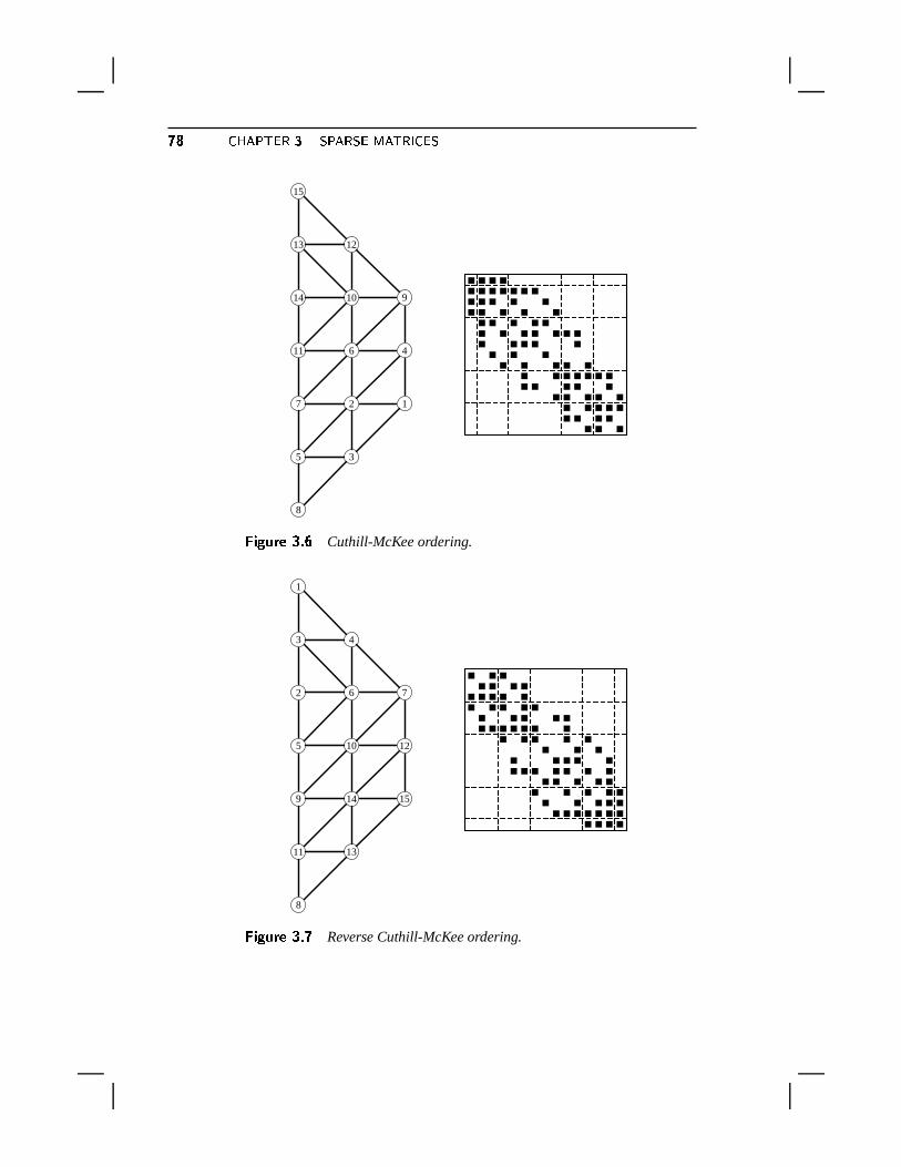
� � �� dK � �

12

3

4

5

6

7

8

910

11

1213

14

15

, � �� 6 � Cuthill-McKee ordering.

1

2

3 4

5

6 7

8

9

10

11

12

13

14 15

, � �� 6 � Reverse Cuthill-McKee ordering.

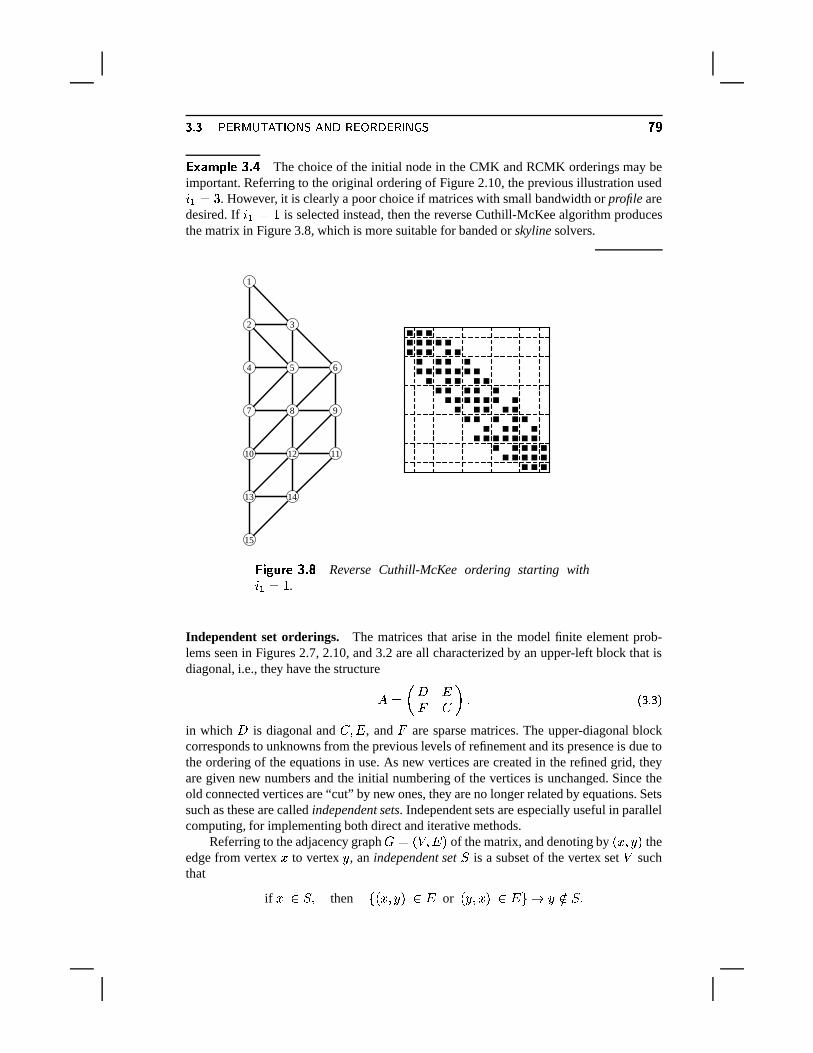
�� ^K � � �� @n �� dn �dK �� 6 � The choice of the initial node in the CMK and RCMK orderings may beimportant. Referring to the original ordering of Figure 2.10, the previous illustration used� � � � . However, it is clearly a poor choice if matrices with small bandwidth or profile aredesired. If � � � � is selected instead, then the reverse Cuthill-McKee algorithm producesthe matrix in Figure 3.8, which is more suitable for banded or skyline solvers.

1

2 3

4 5 6

7 8 9

10 1112

13 14

15

, � �� 6 � Reverse Cuthill-McKee ordering starting with� � �� .

Independent set orderings. The matrices that arise in the model finite element prob-lems seen in Figures 2.7, 2.10, and 3.2 are all characterized by an upper-left block that isdiagonal, i.e., they have the structure

� � � % �� [J � �

in which % is diagonal and � � � , and�

are sparse matrices. The upper-diagonal blockcorresponds to unknowns from the previous levels of refinement and its presence is due tothe ordering of the equations in use. As new vertices are created in the refined grid, theyare given new numbers and the initial numbering of the vertices is unchanged. Since theold connected vertices are “cut” by new ones, they are no longer related by equations. Setssuch as these are called independent sets. Independent sets are especially useful in parallelcomputing, for implementing both direct and iterative methods.

Referring to the adjacency graph � � * � � � + of the matrix, and denoting by *�x�� + theedge from vertex � to vertex � , an independent set � is a subset of the vertex set � suchthat

if � � � � then �%*�x�� + � � or *��y�� + � � � � � ��

� � �� dK � �

To explain this in words: Elements of � are not allowed to be connected to other elementsof � either by incoming or outgoing edges. An independent set is maximal if it cannot beaugmented by elements in its complement to form a larger independent set. Note that amaximal independent set is by no means the largest possible independent set that can befound. In fact, finding the independent set of maximum cardinal is � -hard [132]. In thefollowing, the term independent set always refers to maximal independent set.

There are a number of simple and inexpensive heuristics for finding large maximalindependent sets. A greedy heuristic traverses the nodes in a given order, and if a node isnot already marked, it selects the node as a new member of � . Then this node is markedalong with its nearest neighbors. Here, a nearest neighbor of a node � means any nodelinked to � by an incoming or an outgoing edge.

�� 93/� .8�P�� 6 �� * *,�� &�� &�� 1. Set � � � .2. For �}�O�;�+�z��E� ~ Do:3. If node � is not marked then4. � � �� #� �5. Mark � and all its nearest neighbors6. EndIf7. EndDo

In the above algorithm, the nodes are traversed in the natural order �;�+�u��E� ~ , but theycan also be traversed in any permutation �� 2� � � of �Y�[�<�u��#� ~ � . Since the size of thereduced system is ~ ! � � � , it is reasonable to try to maximize the size of � in order to obtaina small reduced system. It is possible to give a rough idea of the size of � . Assume that themaximum degree of each node does not exceed � . Whenever the above algorithm acceptsa node as a new member of � , it potentially puts all its nearest neighbors, i.e., at most �nodes, in the complement of � . Therefore, if � is the size of � , the size of its complement,~ ! � , is such that ~ ! � �� , and as a result,

� � ~� �� This lower bound can be improved slightly by replacing � with the maximum degree � � ofall the vertices that constitute � . This results in the inequality

� � ~� �� which suggests that it may be a good idea to first visit the nodes with smaller degrees. Infact, this observation leads to a general heuristic regarding a good order of traversal. Thealgorithm can be viewed as follows: Each time a node is visited, remove it and its nearestneighbors from the graph, and then visit a node from the remaining graph. Continue in thesame manner until all nodes are exhausted. Every node that is visited is a member of � andits nearest neighbors are members of 3� . As result, if � � is the degree of the node visited atstep � , adjusted for all the edge deletions resulting from the previous visitation steps, thenthe number ~ � of nodes that are left at step � satisfies the relation

~ �g� ~ � � � ! � �*!��;�

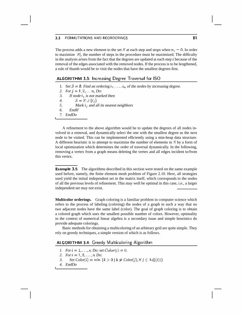
�� ^K � � �� @n �� dn �dK �� y�

The process adds a new element to the set � at each step and stops when ~ � � % . In orderto maximize

� � � , the number of steps in the procedure must be maximized. The difficultyin the analysis arises from the fact that the degrees are updated at each step � because of theremoval of the edges associated with the removed nodes. If the process is to be lengthened,a rule of thumb would be to visit the nodes that have the smallest degrees first.

�� 3/� .q�P�� 6 � � �/� * �� * �� * * � � �� *� � �� &�� 1. Set � � � . Find an ordering � � ��2� � of the nodes by increasing degree.2. For �/�O�;�+�u�� ~ , Do:3. If node � � is not marked then4. � � � � �� 5. Mark � � and all its nearest neighbors6. EndIf7. EndDo

A refinement to the above algorithm would be to update the degrees of all nodes in-volved in a removal, and dynamically select the one with the smallest degree as the nextnode to be visited. This can be implemented efficiently using a min-heap data structure.A different heuristic is to attempt to maximize the number of elements in � by a form oflocal optimization which determines the order of traversal dynamically. In the following,removing a vertex from a graph means deleting the vertex and all edges incident to/fromthis vertex.

� �� 6 � The algorithms described in this section were tested on the same exampleused before, namely, the finite element mesh problem of Figure 2.10. Here, all strategiesused yield the initial independent set in the matrix itself, which corresponds to the nodesof all the previous levels of refinement. This may well be optimal in this case, i.e., a largerindependent set may not exist.

Multicolor orderings. Graph coloring is a familiar problem in computer science whichrefers to the process of labeling (coloring) the nodes of a graph in such a way that notwo adjacent nodes have the same label (color). The goal of graph coloring is to obtaina colored graph which uses the smallest possible number of colors. However, optimalityin the context of numerical linear algebra is a secondary issue and simple heuristics doprovide adequate colorings.

Basic methods for obtaining a multicoloring of an arbitrary grid are quite simple. Theyrely on greedy techniques, a simple version of which is as follows.

�� 3/� .q�P�� 6 � �� *,*,�� ,&�� &�� &��

1. For �@��;��E� ~ Do: set � 3� � *r� + �&% .2. For �@��;�+�u��#� ~ Do:3. Set Color *r� + � � � � � � � % � � � Color *8� + ��>� � � �� *w� +-+ �4. EndDo

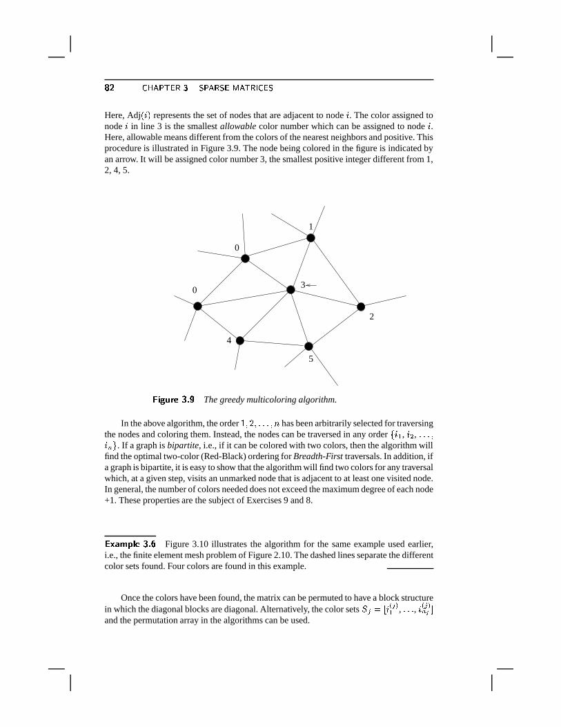
�� dK � �

Here, Adj *w� + represents the set of nodes that are adjacent to node � . The color assigned tonode � in line 3 is the smallest allowable color number which can be assigned to node � .Here, allowable means different from the colors of the nearest neighbors and positive. Thisprocedure is illustrated in Figure 3.9. The node being colored in the figure is indicated byan arrow. It will be assigned color number 3, the smallest positive integer different from 1,2, 4, 5.

3

4

5

2

1

0

0

, � �� 6 � The greedy multicoloring algorithm.

In the above algorithm, the order �;�+�z��#� ~ has been arbitrarily selected for traversingthe nodes and coloring them. Instead, the nodes can be traversed in any order �� , � $ , �� . If a graph is bipartite, i.e., if it can be colored with two colors, then the algorithm willfind the optimal two-color (Red-Black) ordering for Breadth-First traversals. In addition, ifa graph is bipartite, it is easy to show that the algorithm will find two colors for any traversalwhich, at a given step, visits an unmarked node that is adjacent to at least one visited node.In general, the number of colors needed does not exceed the maximum degree of each node+1. These properties are the subject of Exercises 9 and 8.

� �� 6 � Figure 3.10 illustrates the algorithm for the same example used earlier,i.e., the finite element mesh problem of Figure 2.10. The dashed lines separate the differentcolor sets found. Four colors are found in this example.

Once the colors have been found, the matrix can be permuted to have a block structurein which the diagonal blocks are diagonal. Alternatively, the color sets � �:� � � � � �� , �� , � � � �� !and the permutation array in the algorithms can be used.

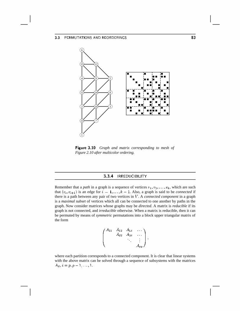
�� ^K � � �� @n �� dn �dK ��

1

2 3

4 5

6

7

8

9

10

11

12

13

14

15

, � �� 6T�� Graph and matrix corresponding to mesh ofFigure 2.10 after multicolor ordering.

�� *��

Remember that a path in a graph is a sequence of vertices � � � � $)�� , which are suchthat * � � � � � " � + is an edge for �}� �[��E� � !O� . Also, a graph is said to be connected ifthere is a path between any pair of two vertices in � . A connected component in a graphis a maximal subset of vertices which all can be connected to one another by paths in thegraph. Now consider matrices whose graphs may be directed. A matrix is reducible if itsgraph is not connected, and irreducible otherwise. When a matrix is reducible, then it canbe permuted by means of symmetric permutations into a block upper triangular matrix ofthe form !""

#� � � � � $ � ��

� $ $ � $ � ��. . .

...� �.�

&('') �

where each partition corresponds to a connected component. It is clear that linear systemswith the above matrix can be solved through a sequence of subsystems with the matrices� �q� , �� ! �[��E�� .

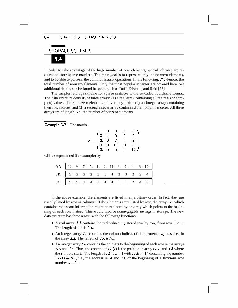
� � �� dK � ��

�7|��

In order to take advantage of the large number of zero elements, special schemes are re-quired to store sparse matrices. The main goal is to represent only the nonzero elements,and to be able to perform the common matrix operations. In the following, �

�denotes the

total number of nonzero elements. Only the most popular schemes are covered here, butadditional details can be found in books such as Duff, Erisman, and Reid [77].

The simplest storage scheme for sparse matrices is the so-called coordinate format.The data structure consists of three arrays: (1) a real array containing all the real (or com-plex) values of the nonzero elements of � in any order; (2) an integer array containingtheir row indices; and (3) a second integer array containing their column indices. All threearrays are of length �

�, the number of nonzero elements.

� �� 6 � The matrix

� �!"""#�[� %p� %p� �u� %z�� %p� � � %z��z� %p� � � �z� �z�%z� %p� � %p��[�;� %z�%z� %p� %p� %z� ��u�

& ''')

will be represented (for example) by

AA 12. 9. 7. 5. 1. 2. 11. 3. 6. 4. 8. 10.

JR 5 3 3 2 1 1 4 2 3 2 3 4

JC 5 5 3 4 1 4 4 1 1 2 4 3

In the above example, the elements are listed in an arbitrary order. In fact, they areusually listed by row or columns. If the elements were listed by row, the array � � whichcontains redundant information might be replaced by an array which points to the begin-ning of each row instead. This would involve nonnegligible savings in storage. The newdata structure has three arrays with the following functions:� A real array �� contains the real values �z�0� stored row by row, from row 1 to ~ .

The length of �:� is ��.� An integer array � � contains the column indices of the elements � �F� as stored in

the array �� . The length of � � is Nz.� An integer array� � contains the pointers to the beginning of each row in the arrays�� and � � . Thus, the content of

� � *r� + is the position in arrays �� and � � wherethe � -th row starts. The length of

� � is ~,� � with� � * ~,� � + containing the number� � *2� + � �

�, i.e., the address in � and � � of the beginning of a fictitious row

number ~Z� � .

��

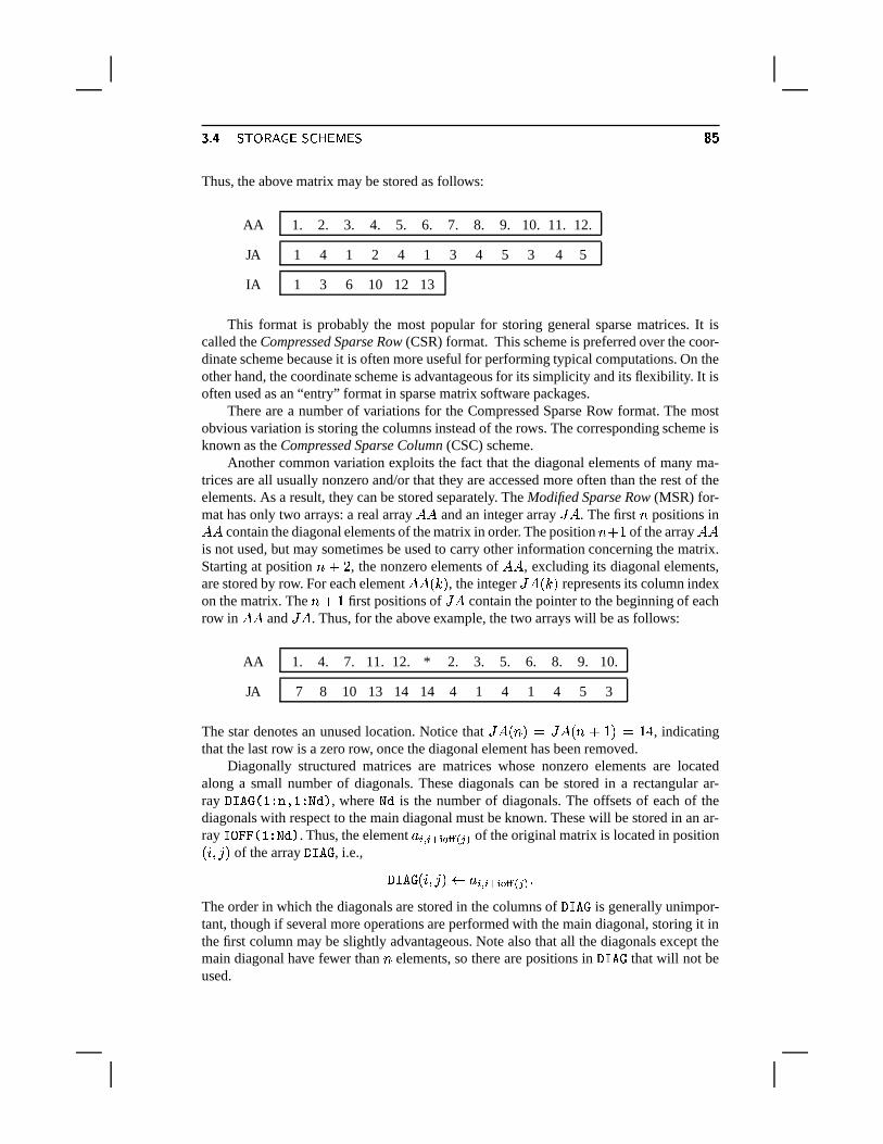
Thus, the above matrix may be stored as follows:

AA 1. 2. 3. 4. 5. 6. 7. 8. 9. 10. 11. 12.

JA 1 4 1 2 4 1 3 4 5 3 4 5

IA 1 3 6 10 12 13

This format is probably the most popular for storing general sparse matrices. It iscalled the Compressed Sparse Row (CSR) format. This scheme is preferred over the coor-dinate scheme because it is often more useful for performing typical computations. On theother hand, the coordinate scheme is advantageous for its simplicity and its flexibility. It isoften used as an “entry” format in sparse matrix software packages.

There are a number of variations for the Compressed Sparse Row format. The mostobvious variation is storing the columns instead of the rows. The corresponding scheme isknown as the Compressed Sparse Column (CSC) scheme.

Another common variation exploits the fact that the diagonal elements of many ma-trices are all usually nonzero and/or that they are accessed more often than the rest of theelements. As a result, they can be stored separately. The Modified Sparse Row (MSR) for-mat has only two arrays: a real array �:� and an integer array � � . The first ~ positions in�:� contain the diagonal elements of the matrix in order. The position ~^� � of the array ��is not used, but may sometimes be used to carry other information concerning the matrix.Starting at position ~D� � , the nonzero elements of �:� , excluding its diagonal elements,are stored by row. For each element �� * � + , the integer � � * � + represents its column indexon the matrix. The ~?� � first positions of � � contain the pointer to the beginning of eachrow in �:� and � � . Thus, for the above example, the two arrays will be as follows:

AA 1. 4. 7. 11. 12. * 2. 3. 5. 6. 8. 9. 10.

JA 7 8 10 13 14 14 4 1 4 1 4 5 3

The star denotes an unused location. Notice that � � * ~ + � � � * ~ � � + � � � , indicatingthat the last row is a zero row, once the diagonal element has been removed.

Diagonally structured matrices are matrices whose nonzero elements are locatedalong a small number of diagonals. These diagonals can be stored in a rectangular ar-ray �� , where �� is the number of diagonals. The offsets of each of thediagonals with respect to the main diagonal must be known. These will be stored in an ar-ray �� . Thus, the element � � � � "�� of the original matrix is located in position*r�<�=� + of the array �� , i.e.,

�� *w�+�H� + � � � � � "�� !� � � � �The order in which the diagonals are stored in the columns of �� is generally unimpor-tant, though if several more operations are performed with the main diagonal, storing it inthe first column may be slightly advantageous. Note also that all the diagonals except themain diagonal have fewer than ~ elements, so there are positions in �� that will not beused.

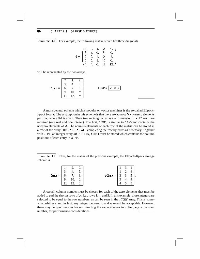
� � �� dK � �� 6 � For example, the following matrix which has three diagonals

� �!"""#�;� %z� �z� %z� %z�� p� %p� � � %z�%p� �z� � � %z� �z�%p� %z� �p�� %z� %z�%p� %z� %p��[�[��A�u�

&(''')

will be represented by the two arrays

�� =

* 1. 2.3. 4. 5.6. 7. 8.9. 10. *11 12. *

�� = -1 0 2 .

A more general scheme which is popular on vector machines is the so-called Ellpack-Itpack format. The assumption in this scheme is that there are at most � ' nonzero elementsper row, where �� is small. Then two rectangular arrays of dimension �� each arerequired (one real and one integer). The first,

� �� , is similar to �� and contains thenonzero elements of � . The nonzero elements of each row of the matrix can be stored ina row of the array

� �� , completing the row by zeros as necessary. Togetherwith

� �� , an integer array �� must be stored which contains the column

positions of each entry in� �� .

� �� 6 � Thus, for the matrix of the previous example, the Ellpack-Itpack storagescheme is

� �� =

1. 2. 0.3. 4. 5.6. 7. 8.9. 10. 0.11 12. 0.

�� =

1 3 11 2 42 3 53 4 44 5 5

.

A certain column number must be chosen for each of the zero elements that must beadded to pad the shorter rows of � , i.e., rows 1, 4, and 5. In this example, those integers areselected to be equal to the row numbers, as can be seen in the �

� �� array. This is some-what arbitrary, and in fact, any integer between � and ~ would be acceptable. However,there may be good reasons for not inserting the same integers too often, e.g. a constantnumber, for performance considerations.

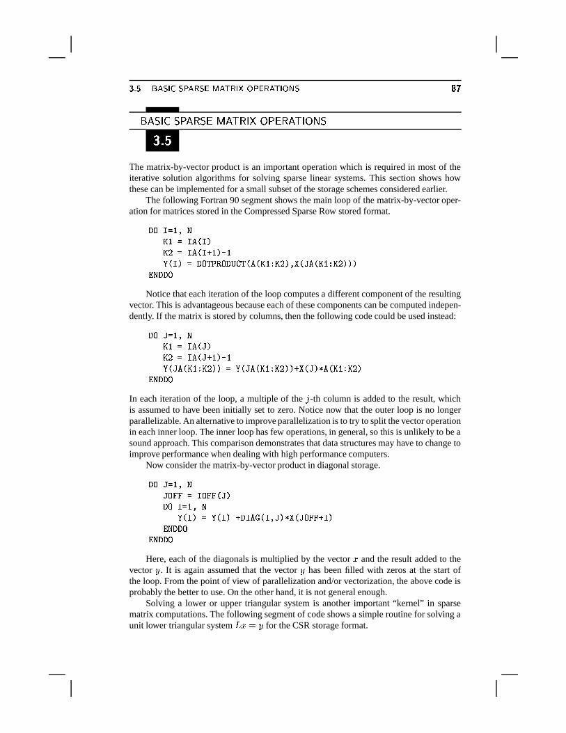
�� pK � � � � �� dK � � � �� ^K � �� ?|��

The matrix-by-vector product is an important operation which is required in most of theiterative solution algorithms for solving sparse linear systems. This section shows howthese can be implemented for a small subset of the storage schemes considered earlier.

The following Fortran 90 segment shows the main loop of the matrix-by-vector oper-ation for matrices stored in the Compressed Sparse Row stored format.

� � �� !��

Notice that each iteration of the loop computes a different component of the resultingvector. This is advantageous because each of these components can be computed indepen-dently. If the matrix is stored by columns, then the following code could be used instead:

� � ��

In each iteration of the loop, a multiple of the � -th column is added to the result, whichis assumed to have been initially set to zero. Notice now that the outer loop is no longerparallelizable. An alternative to improve parallelization is to try to split the vector operationin each inner loop. The inner loop has few operations, in general, so this is unlikely to be asound approach. This comparison demonstrates that data structures may have to change toimprove performance when dealing with high performance computers.

Now consider the matrix-by-vector product in diagonal storage.

� � ��

�� Here, each of the diagonals is multiplied by the vector � and the result added to the

vector � . It is again assumed that the vector � has been filled with zeros at the start ofthe loop. From the point of view of parallelization and/or vectorization, the above code isprobably the better to use. On the other hand, it is not general enough.

Solving a lower or upper triangular system is another important “kernel” in sparsematrix computations. The following segment of code shows a simple routine for solving aunit lower triangular system � �R� � for the CSR storage format.

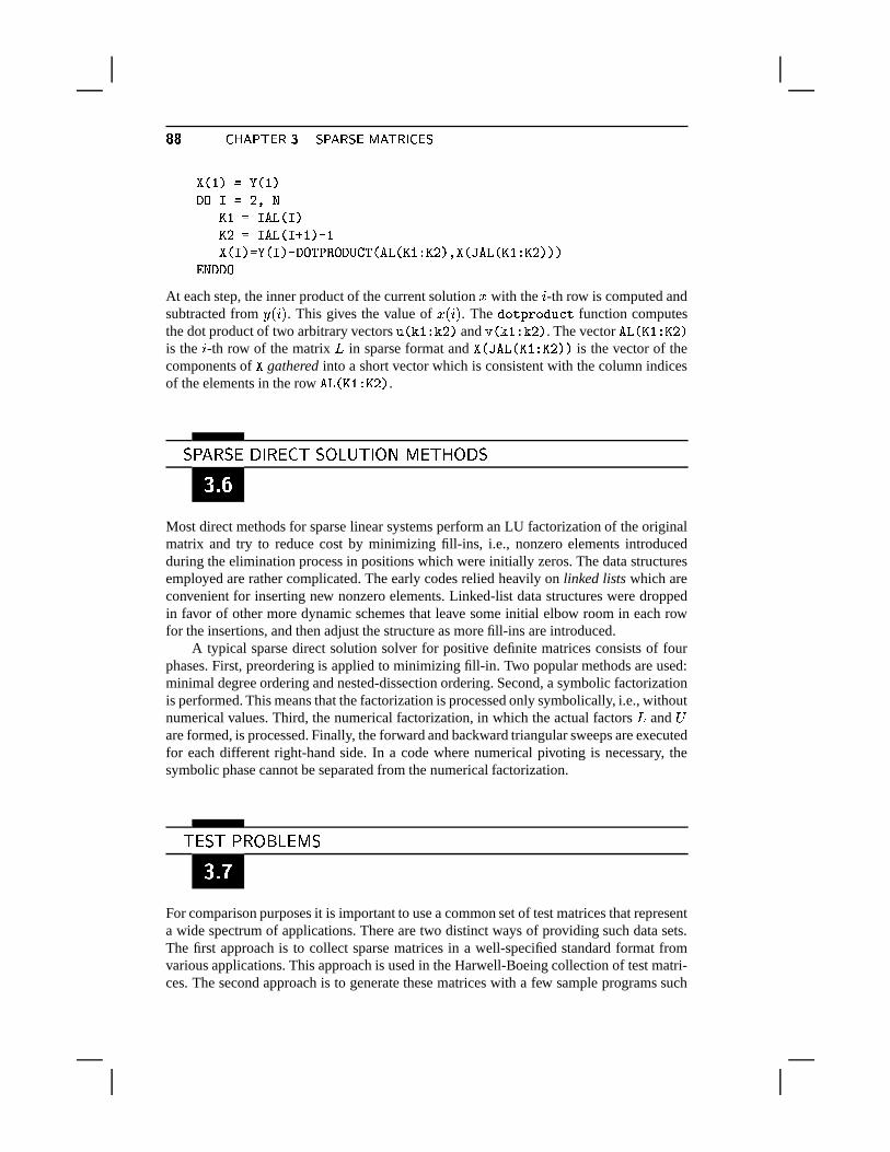
� � �� dK � �

� ��

�� !� � � � � ��

At each step, the inner product of the current solution � with the � -th row is computed andsubtracted from � *w� + . This gives the value of ��*w� + . The �� function computesthe dot product of two arbitrary vectors � �� and �� . The vector � � � � � �� is the � -th row of the matrix � in sparse format and �� is the vector of thecomponents of � gathered into a short vector which is consistent with the column indicesof the elements in the row � � � � � �� .

� ��

�7|��Most direct methods for sparse linear systems perform an LU factorization of the originalmatrix and try to reduce cost by minimizing fill-ins, i.e., nonzero elements introducedduring the elimination process in positions which were initially zeros. The data structuresemployed are rather complicated. The early codes relied heavily on linked lists which areconvenient for inserting new nonzero elements. Linked-list data structures were droppedin favor of other more dynamic schemes that leave some initial elbow room in each rowfor the insertions, and then adjust the structure as more fill-ins are introduced.

A typical sparse direct solution solver for positive definite matrices consists of fourphases. First, preordering is applied to minimizing fill-in. Two popular methods are used:minimal degree ordering and nested-dissection ordering. Second, a symbolic factorizationis performed. This means that the factorization is processed only symbolically, i.e., withoutnumerical values. Third, the numerical factorization, in which the actual factors � and are formed, is processed. Finally, the forward and backward triangular sweeps are executedfor each different right-hand side. In a code where numerical pivoting is necessary, thesymbolic phase cannot be separated from the numerical factorization.

� � �� 7|��

For comparison purposes it is important to use a common set of test matrices that representa wide spectrum of applications. There are two distinct ways of providing such data sets.The first approach is to collect sparse matrices in a well-specified standard format fromvarious applications. This approach is used in the Harwell-Boeing collection of test matri-ces. The second approach is to generate these matrices with a few sample programs such

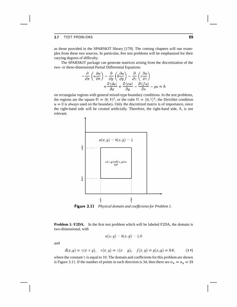
�� 7� � � �as those provided in the SPARSKIT library [179]. The coming chapters will use exam-ples from these two sources. In particular, five test problems will be emphasized for theirvarying degrees of difficulty.

The SPARSKIT package can generate matrices arising from the discretization of thetwo- or three-dimensional Partial Differential Equations

!�� 8� � � !

��8� � � !

�� 8� � �

�� * ' 8 +��

� * � 8 +��

� * � 8 +� � ��8 � �on rectangular regions with general mixed-type boundary conditions. In the test problems,the regions are the square � � * %z�� + $ , or the cube � � *�%z�� + � ; the Dirichlet condition8 � % is always used on the boundary. Only the discretized matrix is of importance, sincethe right-hand side will be created artificially. Therefore, the right-hand side, � , is notrelevant.

��

�

�

�*��g�� + � � *��g�� + ��

��

��

��

��

, � �� 6T�z� Physical domain and coefficients for Problem 1.

Problem 1: F2DA. In the first test problem which will be labeled F2DA, the domain istwo-dimensional, with

� *�x�� + � � *�x�� + ��;� %and

'*�g�� + � � *� � � + � �%*�x�� + � � *�� ! � + � � *�g�� + � � *�x�� + �&%p� %p� � �[J � �where the constant � is equal to 10. The domain and coefficients for this problem are shownis Figure 3.11. If the number of points in each direction is 34, then there are ~ � � ~ � � � �

� � �� dK � �

interior points in each direction and a matrix of size ~ � ~ � �l~ � � � � $ � � %;� � isobtained. In this test example, as well as the other ones described below, the right-handside is generated as

� � � �Y�in which �G� *_�;��[��E�� + / . The initial guess is always taken to be a vector of pseudo-random values.

Problem 2: F2DB. The second test problem is similar to the previous one but involvesdiscontinuous coefficient functions � and � . Here, ~ � � ~ � � � � and the functions'p� �Y� �y� � are also defined by (3.4). However, the functions � and � now both take the value1,000 inside the subsquare of width

�$ centered at (�$ � �$ ), and one elsewhere in the domain,

i.e.,

� *�x�� + � � *�x�� + �� % � ��

��g��

��

Problem 3: F3D. The third test problem is three-dimensional with ~ � � ~ � � ~�� internal mesh points in each direction leading to a problem of size ~ � � %�� . In this case,we take

� *�g��c� � + � � *��g��c� � + �� *�x��c� � + ��' *��g��c� � + � � � � � � � *��g��y� � + � � � � � � �

and � *�x��c� � + � � *�x��c� � + �&%p� %p�The constant � is taken to be equal to 10.0 as before.

The Harwell-Boeing collection is a large data set consisting of test matrices whichhave been contributed by researchers and engineers from many different disciplines. Thesehave often been used for test purposes in the literature [78]. The collection provides a datastructure which constitutes an excellent medium for exchanging matrices. The matrices arestored as ASCII files with a very specific format consisting of a four- or five-line header.Then, the data containing the matrix is stored in CSC format together with any right-hand sides, initial guesses, or exact solutions when available. The SPARSKIT library alsoprovides routines for reading and generating matrices in this format.

Only one matrix from the collection was selected for testing the algorithms describedin the coming chapters. The matrices in the last two test examples are both irregularlystructured.

Problem 4: ORS The matrix selected from the Harwell-Boeing collection is ORSIRR1.This matrix arises from a reservoir engineering problem. Its size is ~ � � % � % and it hasa total of �

� � 6,858 nonzero elements. The original problem is based on a �z� � �u� � �irregular grid. In this case and the next one, the matrices are preprocessed by scaling theirrows and columns.

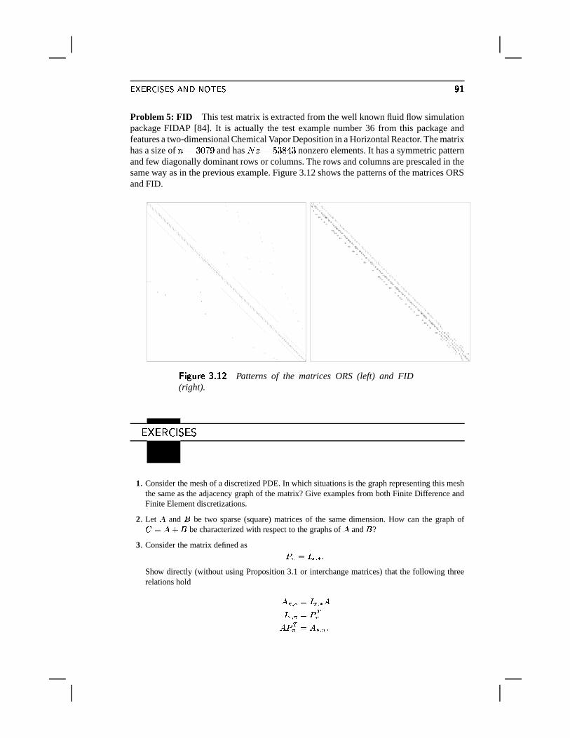
� �� gK � � � �@n � � � � � �Problem 5: FID This test matrix is extracted from the well known fluid flow simulationpackage FIDAP [84]. It is actually the test example number 36 from this package andfeatures a two-dimensional Chemical Vapor Deposition in a Horizontal Reactor. The matrixhas a size of ~ � � % � � and has �

� � � � �� nonzero elements. It has a symmetric patternand few diagonally dominant rows or columns. The rows and columns are prescaled in thesame way as in the previous example. Figure 3.12 shows the patterns of the matrices ORSand FID.

, � �� 6T� � Patterns of the matrices ORS (left) and FID(right).

� � ��

1 Consider the mesh of a discretized PDE. In which situations is the graph representing this meshthe same as the adjacency graph of the matrix? Give examples from both Finite Difference andFinite Element discretizations.

2 Let � and � be two sparse (square) matrices of the same dimension. How can the graph of$$�� be characterized with respect to the graphs of � and � ?

3 Consider the matrix defined asB�� / � #

Show directly (without using Proposition 3.1 or interchange matrices) that the following threerelations hold

�� / � � � � / � �� / � � B 6��"B 6� �� ./ � #

� � �� dK � �

4 Consider the two matrices

��

!""""#�� L�� "�"� �

� �� "�L�� "� � ��"�L�"� � ��"�L�"�"� �

& '''') � �

!""""#� � �L�"�"�� L�"�"�� L�"�"�� "� � �"� �

& '''')

where a � represents an arbitrary nonzero element.� � Show the adjacency graphs of the matrices � , � , �� , and �� . (Assume that there are

no numerical cancellations in computing the products �� and �� ). Since there are zerodiagonal elements, represent explicitly the cycles corresponding to the ? � � � B edges whenthey are present. � Consider the matrix $ � �C� . Give an interpretation of an edge in the graph of $ in termsof edges in the graph of � and � . Verify this answer using the above matrices.

�� Consider the particular case in which � �� . Give an interpretation of an edge in the graphof $ in terms of paths of length two in the graph of � . The paths must take into account thecycles corresponding to nonzero diagonal elements of � .

� � Now consider the case where � � � # . Give an interpretation of an edge in the graph of$$�� & in terms of paths of length three in the graph of � . Generalize the result to arbitrarypowers of � .

5 Consider a � �� matrix which has the pattern

�)�

!""""#��

��

&('''') #

� � Show the adjacency graph of � . � Consider the permutation �� . Show the adjacency graph and new patternfor the matrix obtained from a symmetric permutation of � based on the permutation array � .

6 Consider a matrix which has the pattern

�)�

!""""""""#

��

� ��

� � ��

&('''''''') #

� � Show the adjacency graph of � . (Place the 8 vertices on a circle.) � Consider the permutation � � � � � �� . Show the adjacency graph and newpattern for the matrix obtained from a symmetric permutation of � based on the permutationarray � .

�� Show the adjacency graph and new pattern for the matrix obtained from a reverse Cuthill-McKee ordering of � starting with the node 1. (Assume the vertices adjacent to a givenvertex are always listed in increasing order in the data structure that describes the graph.)

� �� gK � � � �@n � � � � �$� � Find a multicolor ordering for � (give the vertex labels color 1, followed by those for color

2, etc.).

7 Given a five-point finite difference graph, show that the greedy algorithm will always find acoloring of the graph with two colors.

8 Prove that the total number of colors found by the greedy multicoloring algorithm does notexceed � �� , where � �� is the maximum degree of all the vertices of a graph (not countingthe cycles ? � � � B associated with diagonal elements).

9 Consider a graph that is bipartite, i.e., 2-colorable. Assume that the vertices of the graph arecolored by a variant of Algorithm (3.4), in which the nodes are traversed in a certain order� 0 � � # � #F# # � � � .�� Is it true that for any permutation

� 0 � #9#9# � � � the number of colors found will be two? � Consider now a permutation satisfying the following property: for each 2 at least one of the

nodes� 0 � � # � #9#9# � � + . 0 is adjacent to

� + . Show that the algorithm will find a 2-coloring of thegraph.

�� Among the following traversals indicate which ones satisfy the property of the previousquestion: (1) Breadth-First Search, (2) random traversal, (3) traversal defined by

� + = anynode adjacent to

� + . 0 .10 Given a matrix that is irreducible and with a symmetric pattern, show that its structural inverse is

dense. Structural inverse means the pattern of the inverse, regardless of the values, or otherwisestated, is the union of all patterns of the inverses for all possible values. [Hint: Use CayleyHamilton’s theorem and a well known result on powers of adjacency matrices mentioned at theend of Section 3.2.1.]

11 The most economical storage scheme in terms of memory usage is the following variation on thecoordinate format: Store all nonzero values % � + in a real array �� and the corresponding“linear array address” ? � �� B�� 2 in an integer array +1� � �� . The order in which thesecorresponding entries are stored is unimportant as long as they are both in the same position intheir respective arrays. What are the advantages and disadvantages of this data structure? Writea short routine for performing a matrix-by-vector product in this format.

12 Write a FORTRAN code segment to perform the matrix-by-vector product for matrices storedin Ellpack-Itpack format.

13 Write a small subroutine to perform the following operations on a sparse matrix in coordinateformat, diagonal format, and CSR format:�� Count the number of nonzero elements in the main diagonal; � Extract the diagonal whose offset is � ;�� Add a nonzero element in position ? � � 2 B of the matrix (this position may initially contain a

zero or a nonzero element);� � Add a given diagonal to the matrix. What is the most convenient storage scheme for each of

these operations?

14 Linked lists is another popular scheme often used for storing sparse matrices. These allow to linktogether � data items (e.g., elements of a given row) in a large linear array. A starting position isgiven in the array which contains the first element of the set. Then, a link to the next element inthe array is provided from a LINK array.�� Show how to implement this scheme. A linked list is to be used for each row. � What are the main advantages and disadvantages of linked lists?

� � �� dK � �� Write an algorithm to perform a matrix-by-vector product in this format.

NOTES AND REFERENCES. Two good references on sparse matrix computations are the book byGeorge and Liu [104] and the more recent volume by Duff, Erisman, and Reid [77]. These are gearedtoward direct solution methods and the first specializes in symmetric positive definite problems. Alsoof interest are [157] and [163] and the early survey by Duff [76].

Sparse matrix techniques have traditionally been associated with direct solution methods.Clearly, this is now changing rapidly since the sophistication of iterative solution packages isstarting to equal that of direct solvers. The SPARSKIT library, a package for sparse matrixcomputations [179] is currently in its second version and is available through anonymous FTP( �� !�"��# �$#%�& ). Another available software packagewhich emphasizes object-oriented design with the goal of hiding complex data structures fromusers is PETSc [19]. A manipulation package for sparse matrices, similar to SPARSKIT in spirit, isSMMS developed by Alvarado [6].

The idea of the greedy multicoloring algorithm is known in Finite Element techniques (to colorelements); see, e.g., Benantar and Flaherty [23]. Wu [229] presents the greedy algorithm for multi-coloring vertices and uses it for SOR type iterations, see also [182]. The effect of multicoloring hasbeen extensively studied by Adams [2, 3] and Poole and Ortega [164]. Interesting results regardingmulticoloring in the context of finite elements based on quad-tree structures have been obtained byBenantar and Flaherty [23] who show, in particular, that with this structure a maximum of six colorsis required.

Documents

Iterative methods for sparse linear systems (PDF)saad/PS/iter1.pdf · Iterative Methods for Sparse Linear Systems ... Iterative methods for solving general, ... ments revolutionized