Imaging using ionizing radiations

IV – Positron Emission Tomography

Slides are courtesy of David Brasse ESIPAP, March 2017

Ziad El Bitar ziad.elbitar@iphc.cnrs.fr

Institut Pluridisciplinaire Hubert Curien, Strasbourg

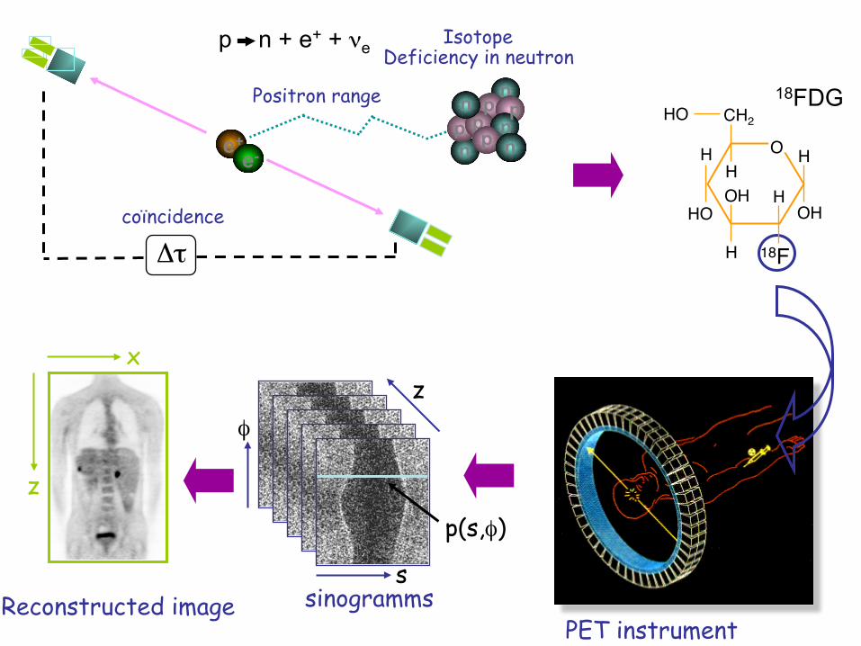
Isotope Deficiency in neutron

n

n p p p p

n p

n

n

Δτcoïncidence

Positron range

e+ e-

p n + e+ + νe

O H

OH

CH2HO

HO

H

H

HHOH

18F

18FDG

PET instrument sinogramms

p(s,φ)

s

z φ

Reconstructed image

z

x

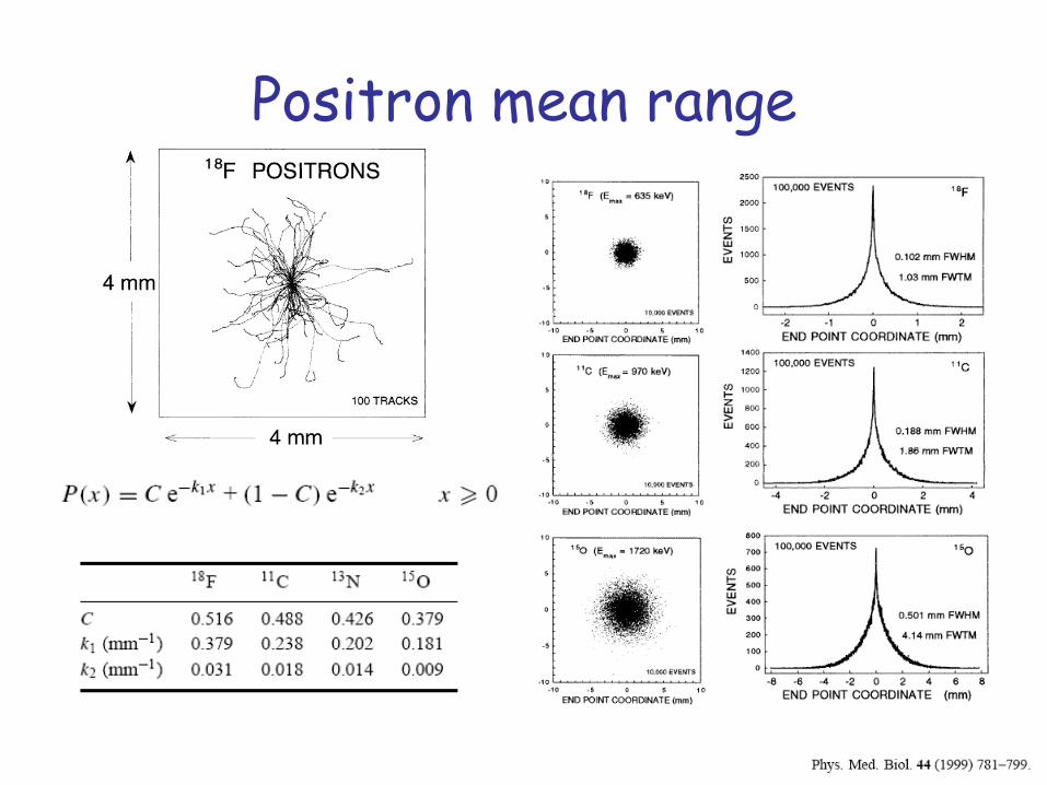
Positron mean range

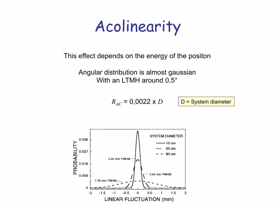
Acolinearity

RAC = 0,0022 x D

This effect depends on the energy of the positon

Angular distribution is almost gaussian With an LTMH around 0,5°

D = System diameter

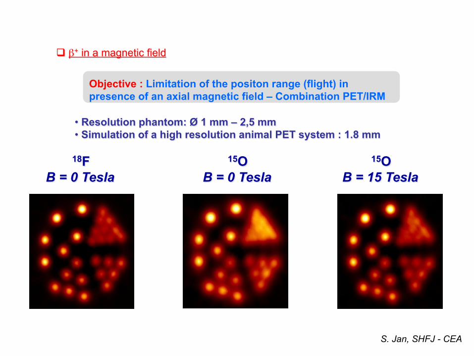
Objective : Limitation of the positon range (flight) in presence of an axial magnetic field – Combination PET/IRM

15O B = 0 Tesla

18F B = 0 Tesla

15O B = 15 Tesla

q  β+ in a magnetic field

•  Resolution phantom: Ø 1 mm – 2,5 mm •  Simulation of a high resolution animal PET system : 1.8 mm

S. Jan, SHFJ - CEA

Physical principles: short remindr

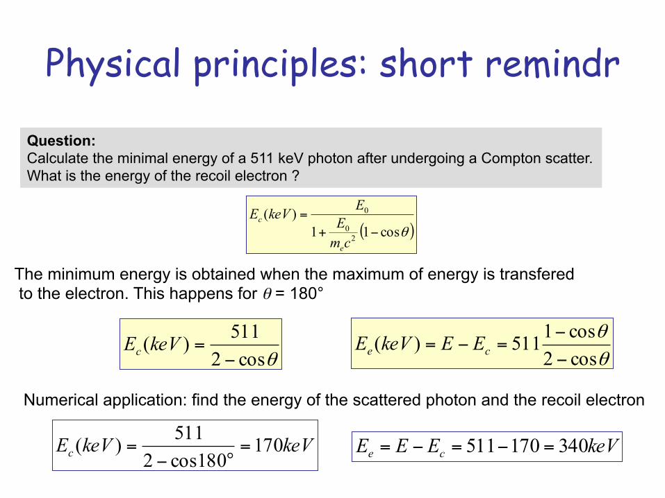
Question: Calculate the minimal energy of a 511 keV photon after undergoing a Compton scatter. What is the energy of the recoil electron ?

θcos2511)(−

=keVEc

keVEEE ce 340170511 =−=−=

The minimum energy is obtained when the maximum of energy is transfered to the electron. This happens for θ = 180°

Numerical application: find the energy of the scattered photon and the recoil electron

keVkeVEc 170180cos2

511)( =°−

=

θθ

cos2cos1511)(

−−

=−= ce EEkeVE

( )θcos11)(

20

0

−+=

cmEEkeVE

e

c

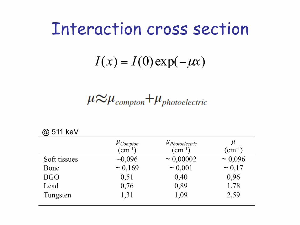
Interaction cross section

)exp()0()( xIxI µ−=

Soft tissues Bone BGO Lead Tungsten

µCompton (cm-1) ~0,096 ~ 0,169

0,51 0,76 1,31

µPhotoelectric (cm-1)

~ 0,00002 ~ 0,001

0,40 0,89 1,09

µ (cm-1)

~ 0,096 ~ 0,17 0,96 1,78 2,59

@ 511 keV

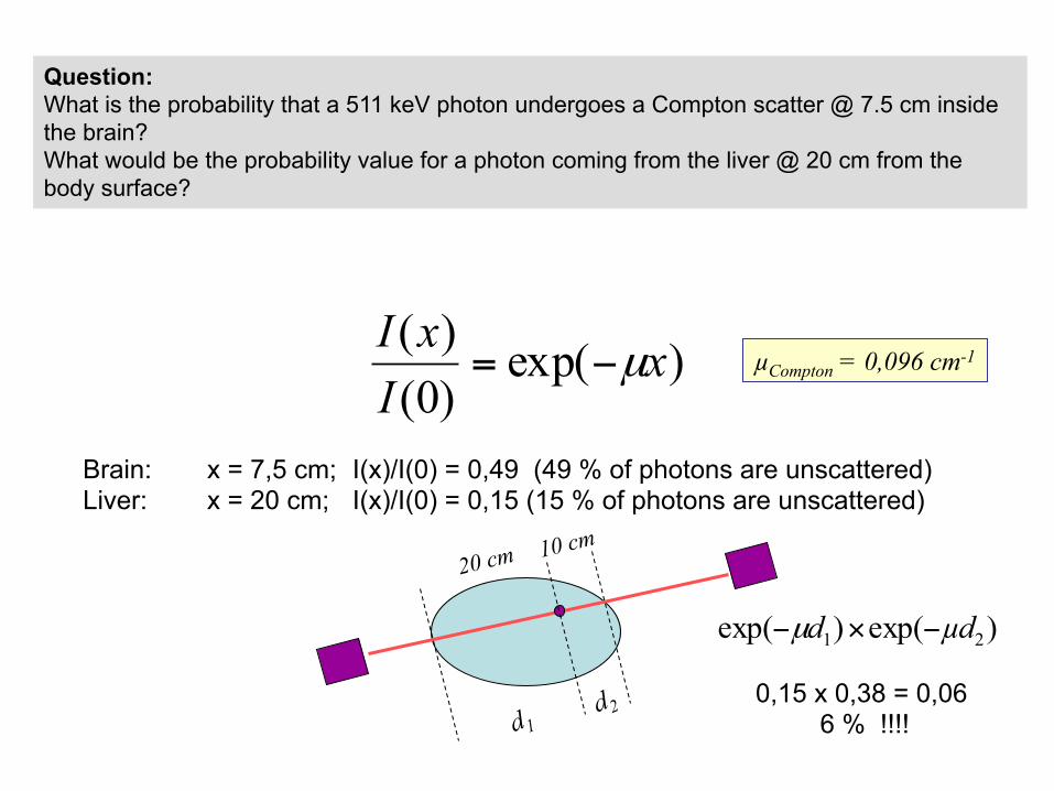
Question: What is the probability that a 511 keV photon undergoes a Compton scatter @ 7.5 cm inside the brain? What would be the probability value for a photon coming from the liver @ 20 cm from the body surface?

)exp()0()( x

IxI

µ−= µCompton = 0,096 cm-1

Brain: x = 7,5 cm; I(x)/I(0) = 0,49 (49 % of photons are unscattered) Liver: x = 20 cm; I(x)/I(0) = 0,15 (15 % of photons are unscattered)

10 cm 20 cm

)exp()exp( 21 µdd −×−µ

0,15 x 0,38 = 0,06 6 % !!!!

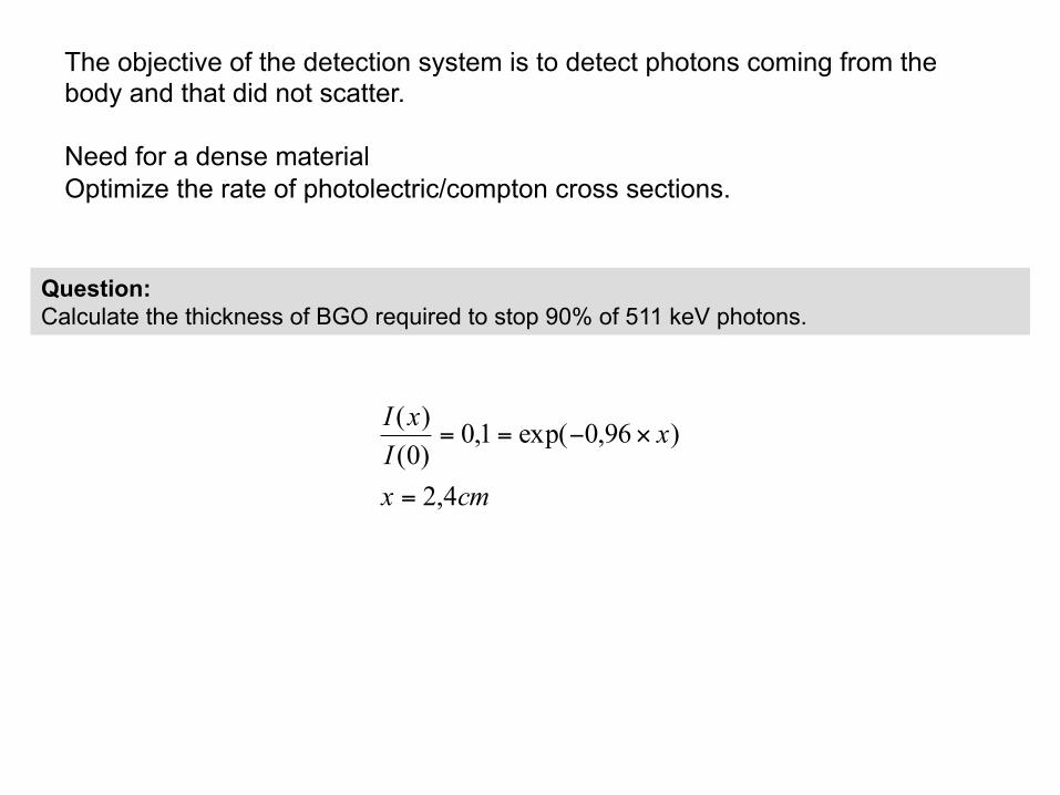
The objective of the detection system is to detect photons coming from the body and that did not scatter. Need for a dense material Optimize the rate of photolectric/compton cross sections.

Question: Calculate the thickness of BGO required to stop 90% of 511 keV photons.

cmx

xIxI

4,2

)96,0exp(1,0)0()(

=

×−==

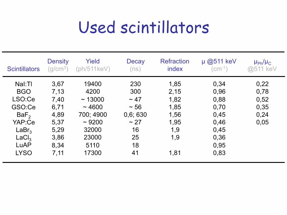
Used scintillators

Density (g/cm3)

3,67 7,13 7,40 6,71 4,89 5,37 5,29 3,86 8,34 7,11

Scintillators

NaI:Tl BGO

LSO:Ce GSO:Ce

BaF2 YAP:Ce LaBr3 LaCl3 LuAP LYSO

Yield (ph/511keV)

19400 4200

~ 13000 ~ 4600

700; 4900 ~ 9200 32000 23000 5110

17300

Decay (ns)

230 300 ~ 47 ~ 56

0,6; 630 ~ 27 16 25 18 41

Refraction index

1,85 2,15 1,82 1,85 1,56 1,95 1,9 1,9

1,81

µ @511 keV (cm-1)

0,34 0,96 0,88 0,70 0,45 0,46 0,45 0,36 0,95 0,83

µPh/µC @511 keV

0,22 0,78 0,52 0,35 0,24 0,05

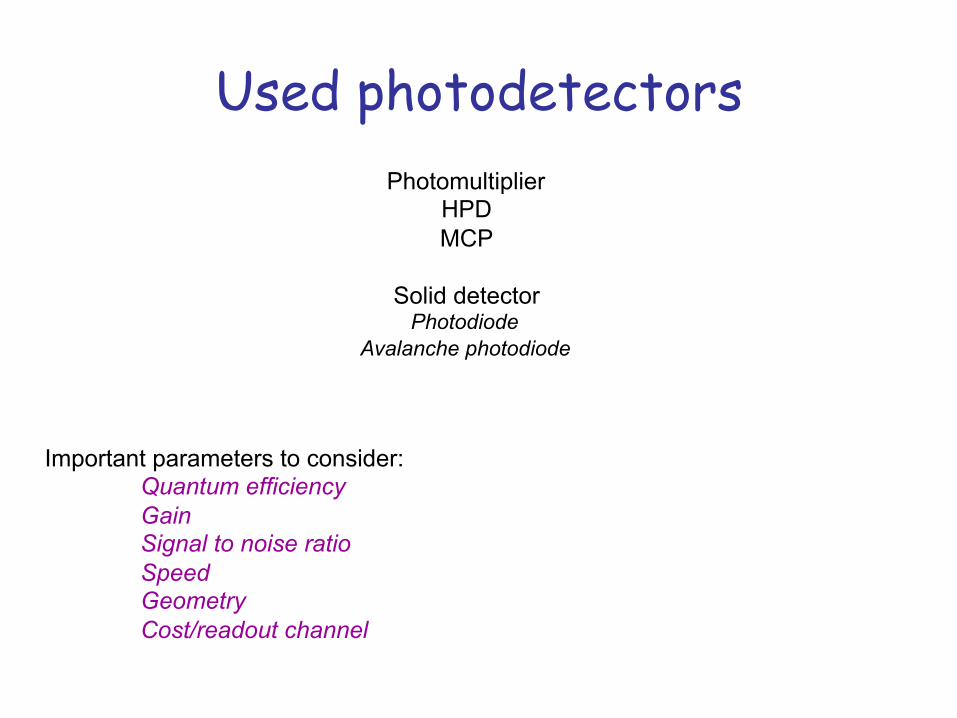
Used photodetectors Photomultiplier

HPD MCP

Solid detector

Photodiode Avalanche photodiode

Important parameters to consider: Quantum efficiency Gain Signal to noise ratio Speed Geometry Cost/readout channel

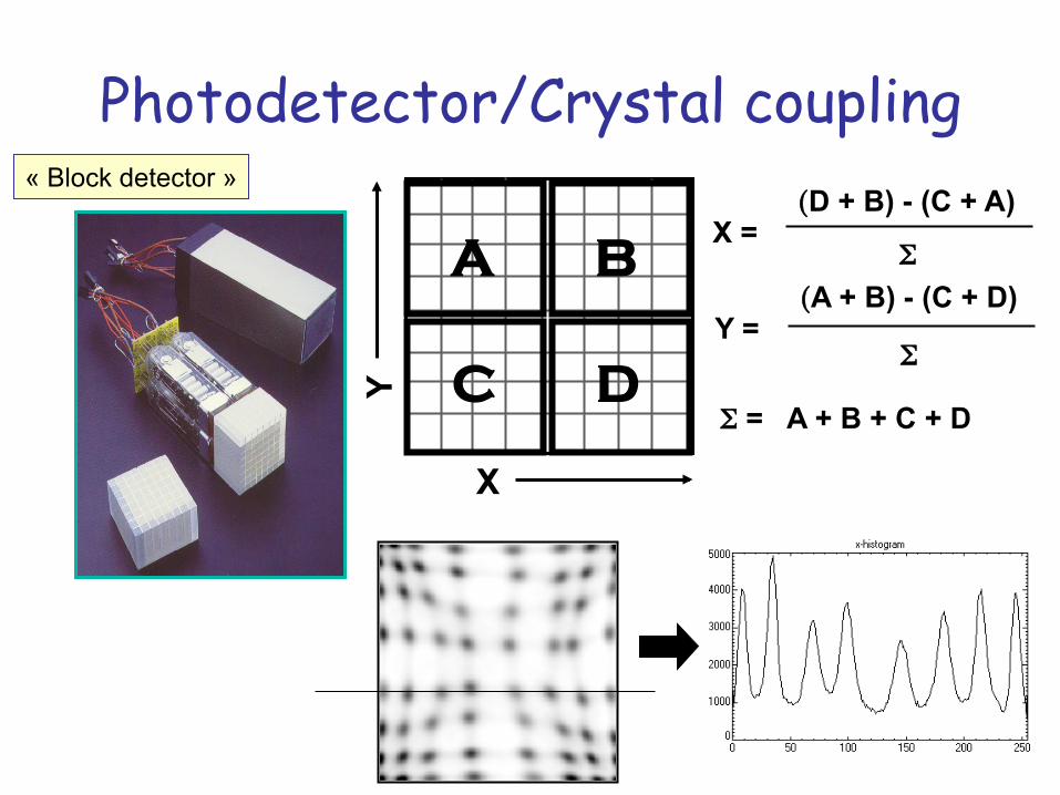
Photodetector/Crystal coupling « Block detector »

A B

C D

X =

Σ = A + B + C + D

Σ

(D + B) - (C + A)

Y = Σ

(A + B) - (C + D)

X

Y

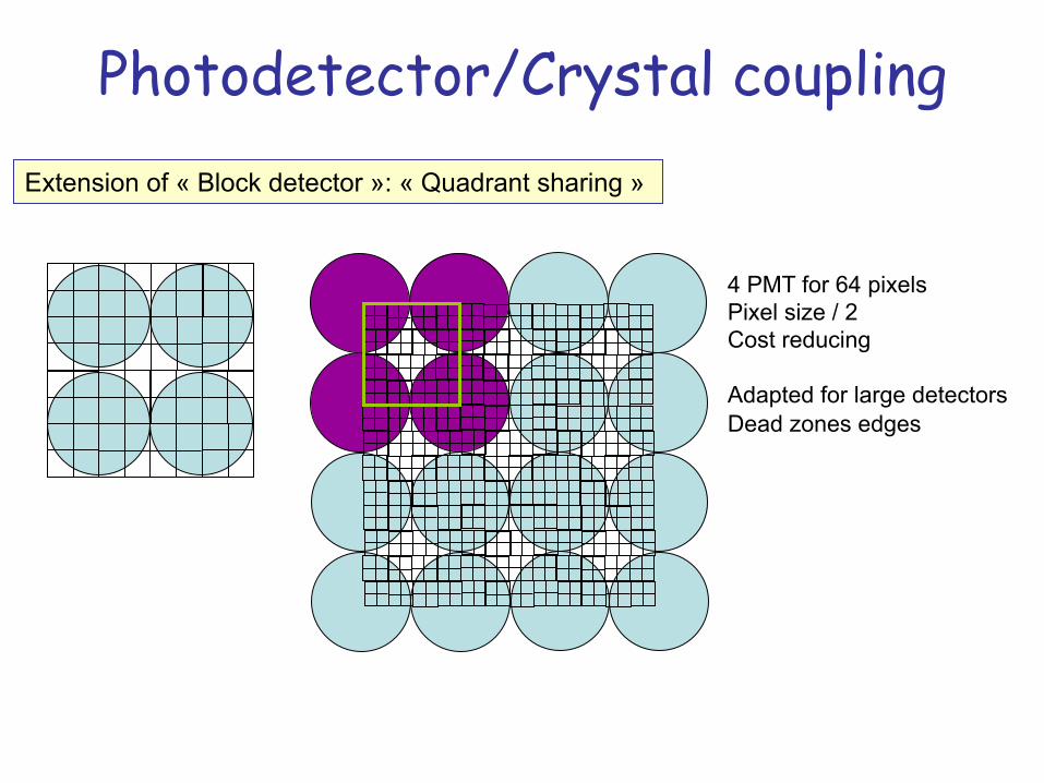
Extension of « Block detector »: « Quadrant sharing »

4 PMT for 64 pixels Pixel size / 2 Cost reducing Adapted for large detectors Dead zones edges

Photodetector/Crystal coupling

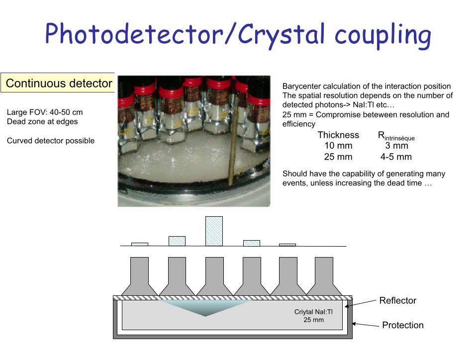
Continuous detector

Criytal NaI:Tl 25 mm

Reflector

Protection

Barycenter calculation of the interaction position The spatial resolution depends on the number of detected photons-> NaI:Tl etc… 25 mm = Compromise beteween resolution and efficiency

Thickness 10 mm 25 mm

Rintrinsèque 3 mm

4-5 mm

Should have the capability of generating many events, unless increasing the dead time …

Large FOV: 40-50 cm Dead zone at edges Curved detector possible

Photodetector/Crystal coupling

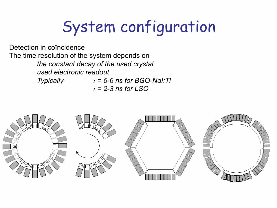
System configuration Detection in coïncidence The time resolution of the system depends on

the constant decay of the used crystal used electronic readout Typically τ = 5-6 ns for BGO-NaI:Tl τ = 2-3 ns for LSO

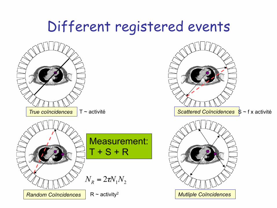
Different registered events

True coïncidences Scattered Coïncidences

Mutliple Coïncidences Random Coïncidences

T ~ activité

212 NNNR τ=

R ~ activity2

S ~ f x activité

Measurement: T + S + R

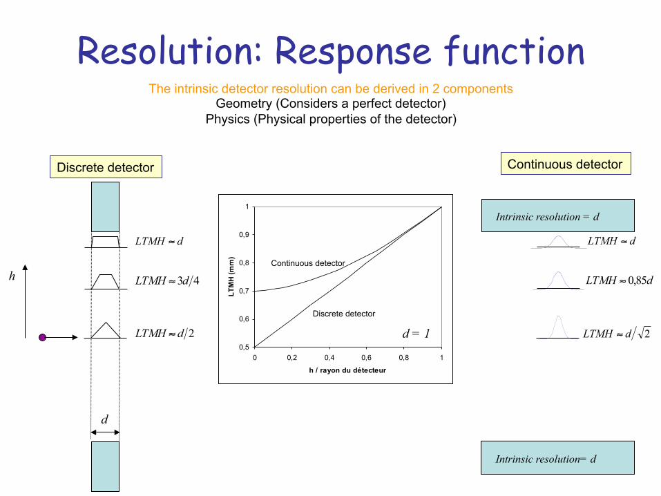
Resolution: Response function The intrinsic detector resolution can be derived in 2 components

Geometry (Considers a perfect detector) Physics (Physical properties of the detector)

2dLTMH ≈

43dLTMH ≈

dLTMH ≈

d

Intrinsic resolution = d

Intrinsic resolution= d

2dLTMH ≈

dLTMH 85,0≈

dLTMH ≈

Discrete detector Continuous detector

h

0,5

0,6

0,7

0,8

0,9

1

0 0,2 0,4 0,6 0,8 1

h / rayon du détecteur

LTM

H (m

m)

d = 1 Discrete detector

Continuous detector

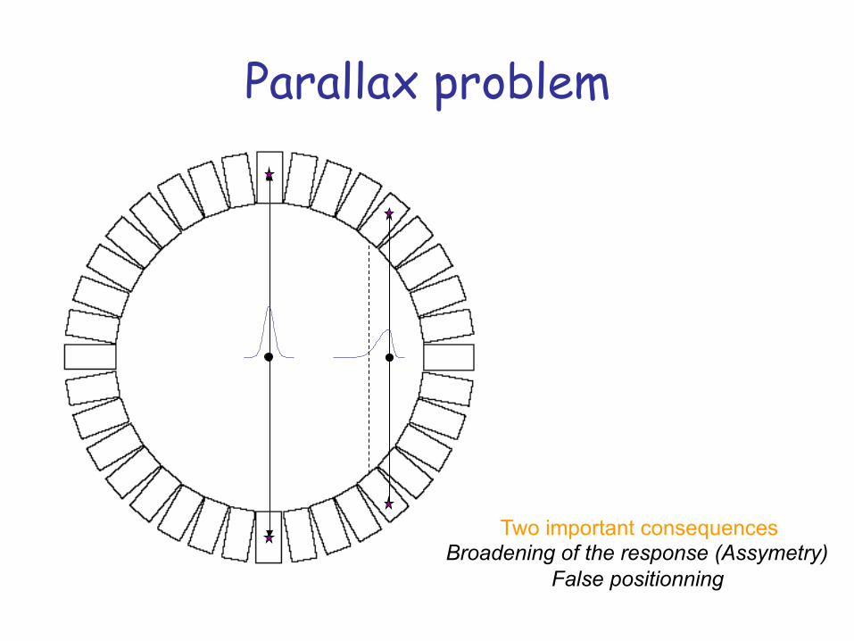
Parallax problem

Two important consequences Broadening of the response (Assymetry)

False positionning

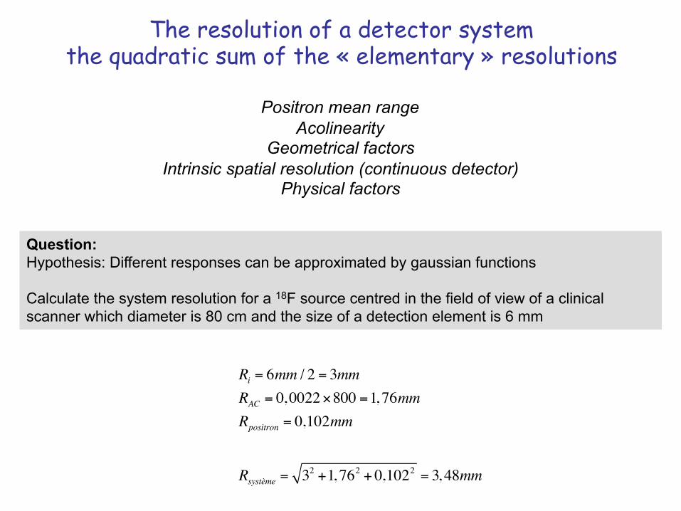
The resolution of a detector system the quadratic sum of the « elementary » resolutions

Positron mean range

Acolinearity Geometrical factors

Intrinsic spatial resolution (continuous detector) Physical factors

Question: Hypothesis: Different responses can be approximated by gaussian functions Calculate the system resolution for a 18F source centred in the field of view of a clinical scanner which diameter is 80 cm and the size of a detection element is 6 mm

Ri = 6mm / 2 = 3mmRAC = 0,0022×800 =1, 76mmRpositron = 0,102mm

Rsystème = 32 +1, 762 + 0,1022 = 3, 48mm

Detection efficiency

The number of registered events is given by The amount of injected radioactivity

Fraction of radioactivity targeting the Region Of Interest (ROI) Duration of the exam

Detection efficiency of the PET system

Unit Cps/Bq/ml

The system efficiency if the product of several factors Detector efficiency @ 511 keV

Detection solid angle Source positionning with respect to detector

The width of the energy window The width of the time window

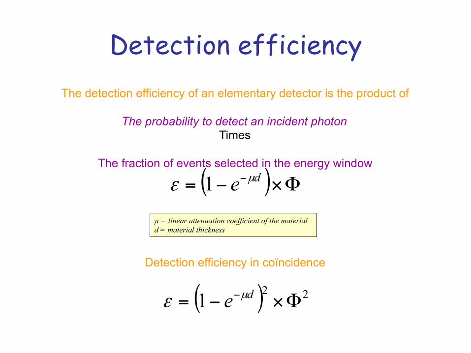
Detection efficiency The detection efficiency of an elementary detector is the product of

The probability to detect an incident photon

Times

The fraction of events selected in the energy window

( ) Φ×−= − de µε 1µ = linear attenuation coefficient of the material d = material thickness

Detection efficiency in coïncidence

( ) 221 Φ×−= − de µε

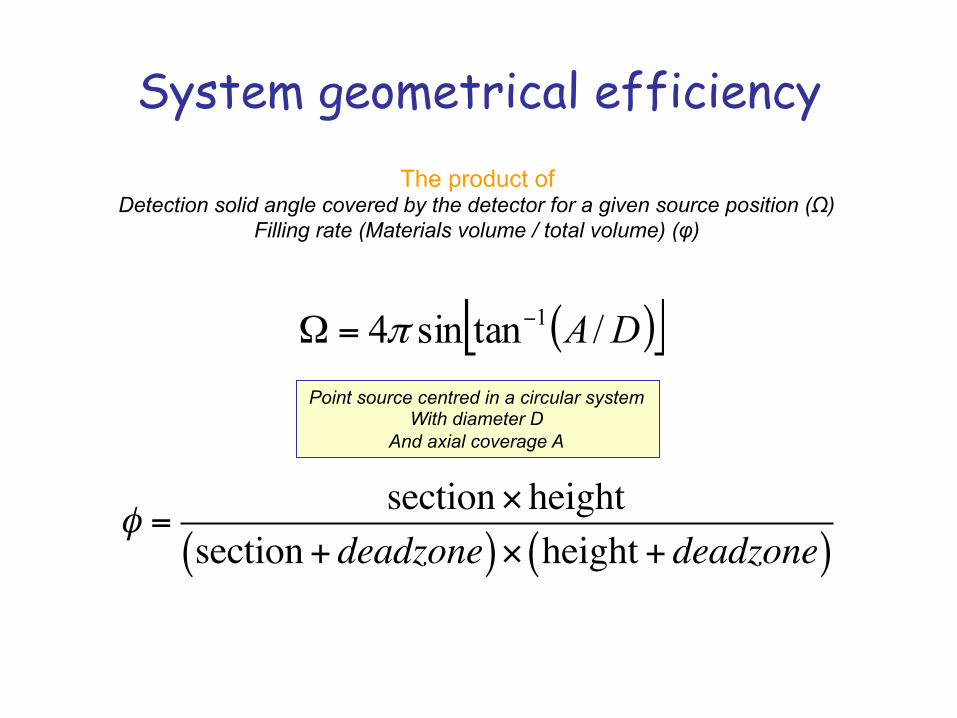
System geometrical efficiency The product of

Detection solid angle covered by the detector for a given source position (Ω) Filling rate (Materials volume / total volume) (φ)

( )[ ]DA /tansin4 1−=Ω π

Point source centred in a circular system With diameter D

And axial coverage A

φ =section× height

section+ deadzone( )× height + deadzone( )

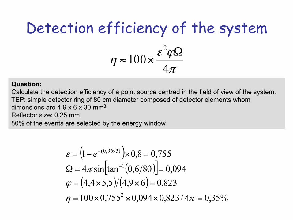
Detection efficiency of the system

πϕε

η4

1002 Ω

×≈

Question: Calculate the detection efficiency of a point source centred in the field of view of the system. TEP: simple detector ring of 80 cm diameter composed of detector elements whom dimensions are 4,9 x 6 x 30 mm3. Reflector size: 0,25 mm 80% of the events are selected by the energy window

( )( )[ ]

( ) ( )%35,04/823,0094,0755,0100

823,069,45,54,4094,0806,0tansin4

755,08,01

2

1

)396,0(

=×××=

=××=

==Ω

=×−=−

×−

πη

ϕ

π

ε e

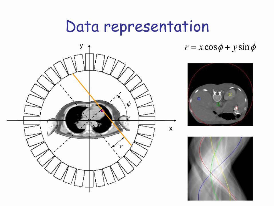
Data representation

x

y

r

φ

φφ sincos yxr +=

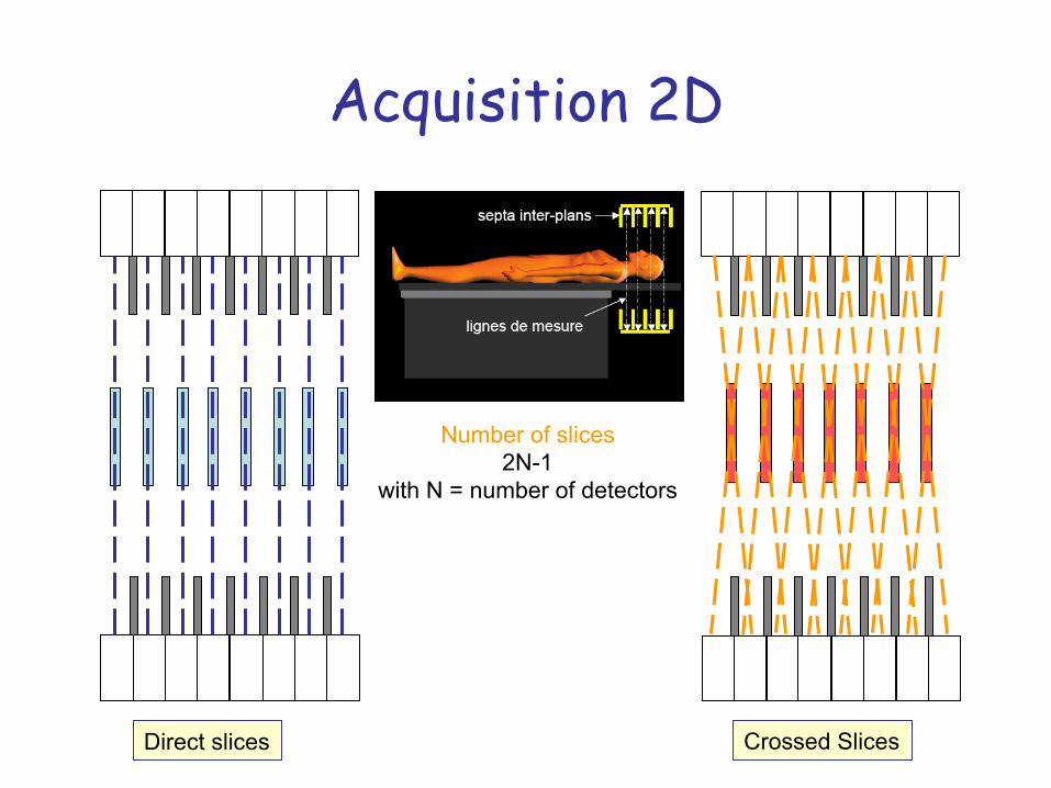
Acquisition 2D

Direct slices Crossed Slices

Number of slices 2N-1

with N = number of detectors

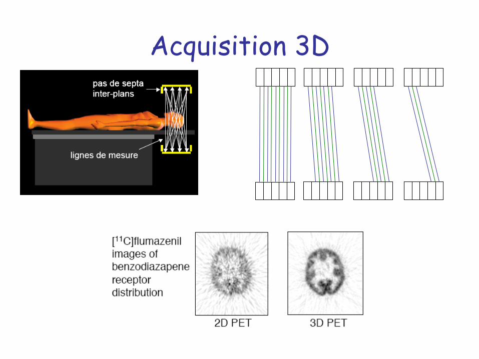
Acquisition 3D

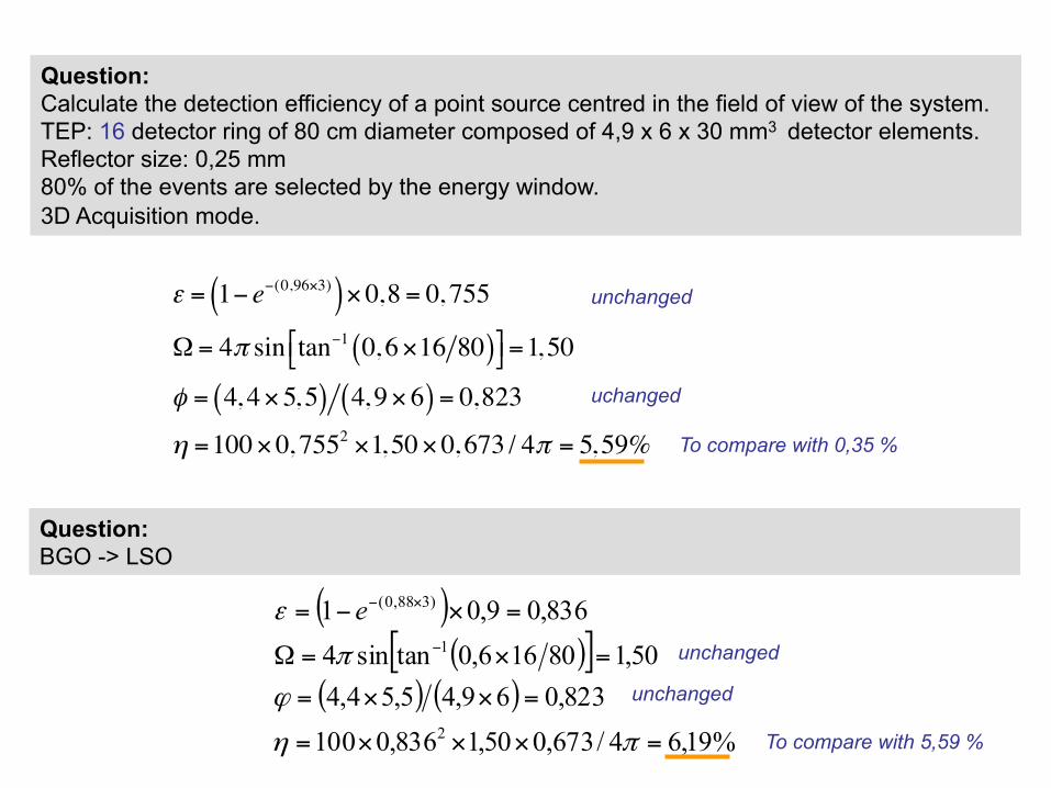
Question: Calculate the detection efficiency of a point source centred in the field of view of the system. TEP: 16 detector ring of 80 cm diameter composed of 4,9 x 6 x 30 mm3 detector elements. Reflector size: 0,25 mm 80% of the events are selected by the energy window. 3D Acquisition mode.

unchanged

uchanged

ε = 1− e−(0,96×3)( )×0,8 = 0, 755Ω = 4π sin tan−1 0, 6×16 80( )$% &'=1,50

φ = 4, 4×5,5( ) 4,9×6( ) = 0,823η =100×0, 7552 ×1,50×0,673 / 4π = 5,59% To compare with 0,35 %

Question: BGO -> LSO

( )( )[ ]

( ) ( )%19,64/673,050,1836,0100

823,069,45,54,450,180166,0tansin4

836,09,01

2

1

)388,0(

=×××=

=××=

=×=Ω

=×−=−

×−

πη

ϕ

π

ε eunchanged

unchanged

To compare with 5,59 %

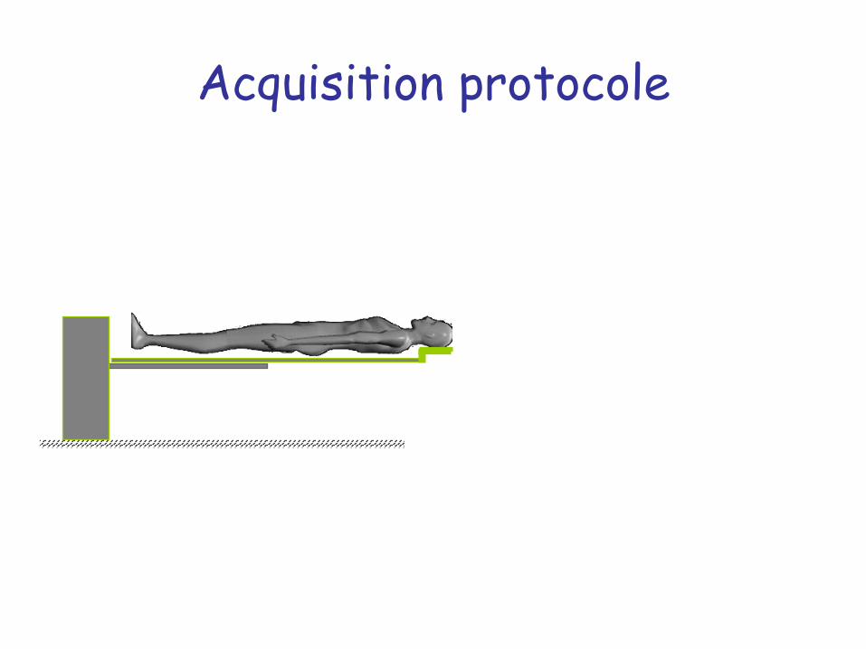
Acquisition protocole

Static or dynamic acquisition in order to cover the whole body.

Data Correction

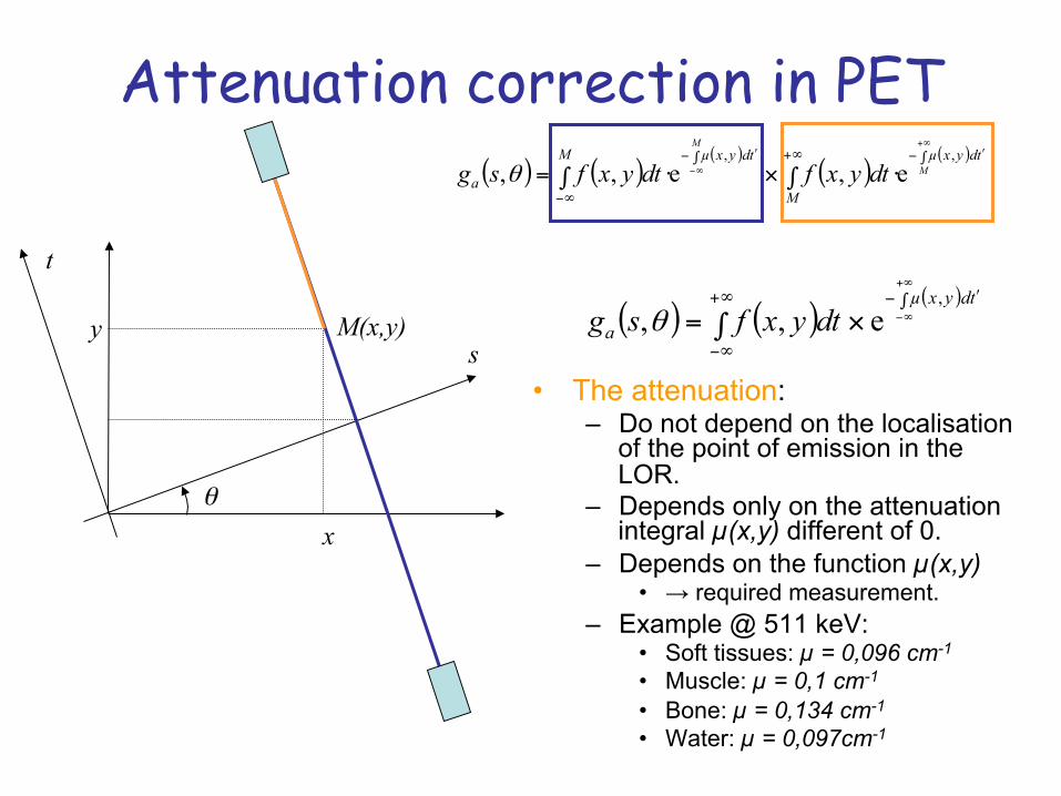
Attenuation correction in PET

•  The attenuation: –  Do not depend on the localisation

of the point of emission in the LOR.

–  Depends only on the attenuation integral µ(x,y) different of 0.

–  Depends on the function µ(x,y) •  → required measurement.

–  Example @ 511 keV: •  Soft tissues: µ = 0,096 cm-1

•  Muscle: µ = 0,1 cm-1

•  Bone: µ = 0,134 cm-1

•  Water: µ = 0,097cm-1

θ

M(x,y)

x

y s

t

( ) ( )( )

( )( )∫ ʹ′−∞+∫ ʹ′−

∞−

+∞

∞− ∫ ⋅×∫ ⋅= M

Mtdyxµ

M

tdyxµM

a dtyxfdtyxfsg,,

e,e,,θ

( ) ( )( )∫ ʹ′−∞+

∞−

+∞

∞−∫ ×=tdyxµ

a dtyxfsg,

e,,θ

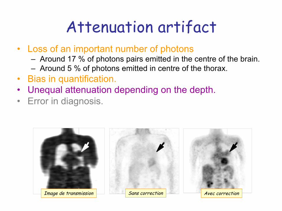
Attenuation artifact •  Loss of an important number of photons

–  Around 17 % of photons pairs emitted in the centre of the brain. –  Around 5 % of photons emitted in centre of the thorax.

•  Bias in quantification. •  Unequal attenuation depending on the depth. •  Error in diagnosis.

Image de transmission Sans correction Avec correction

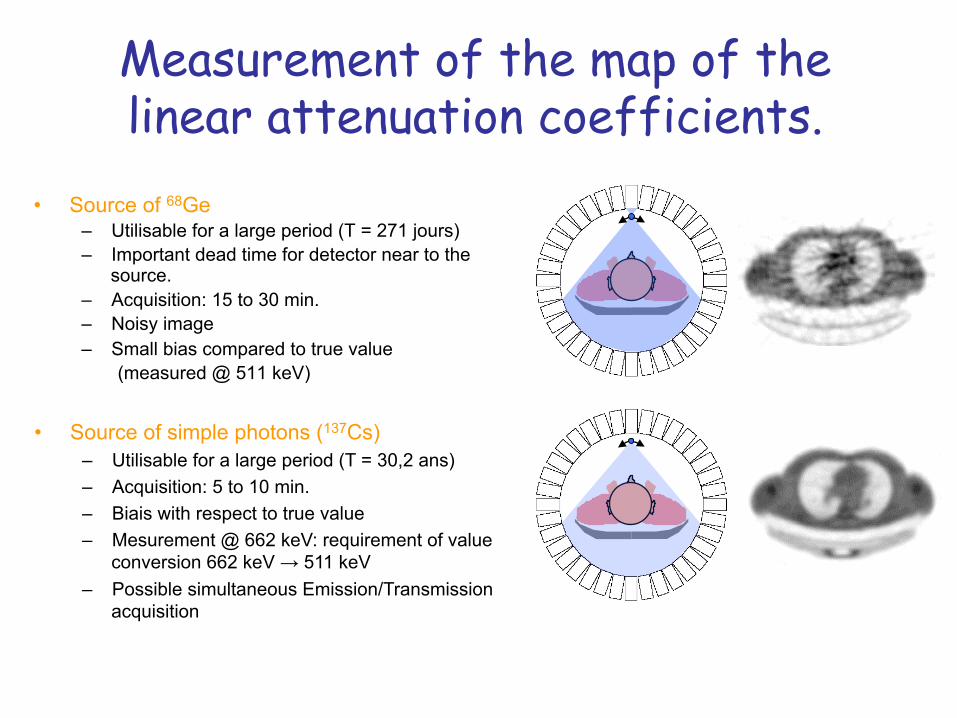
Measurement of the map of the linear attenuation coefficients.

•  Source of 68Ge –  Utilisable for a large period (T = 271 jours) –  Important dead time for detector near to the

source. –  Acquisition: 15 to 30 min. –  Noisy image –  Small bias compared to true value (measured @ 511 keV)

•  Source of simple photons (137Cs) –  Utilisable for a large period (T = 30,2 ans) –  Acquisition: 5 to 10 min. –  Biais with respect to true value –  Mesurement @ 662 keV: requirement of value

conversion 662 keV → 511 keV –  Possible simultaneous Emission/Transmission

acquisition

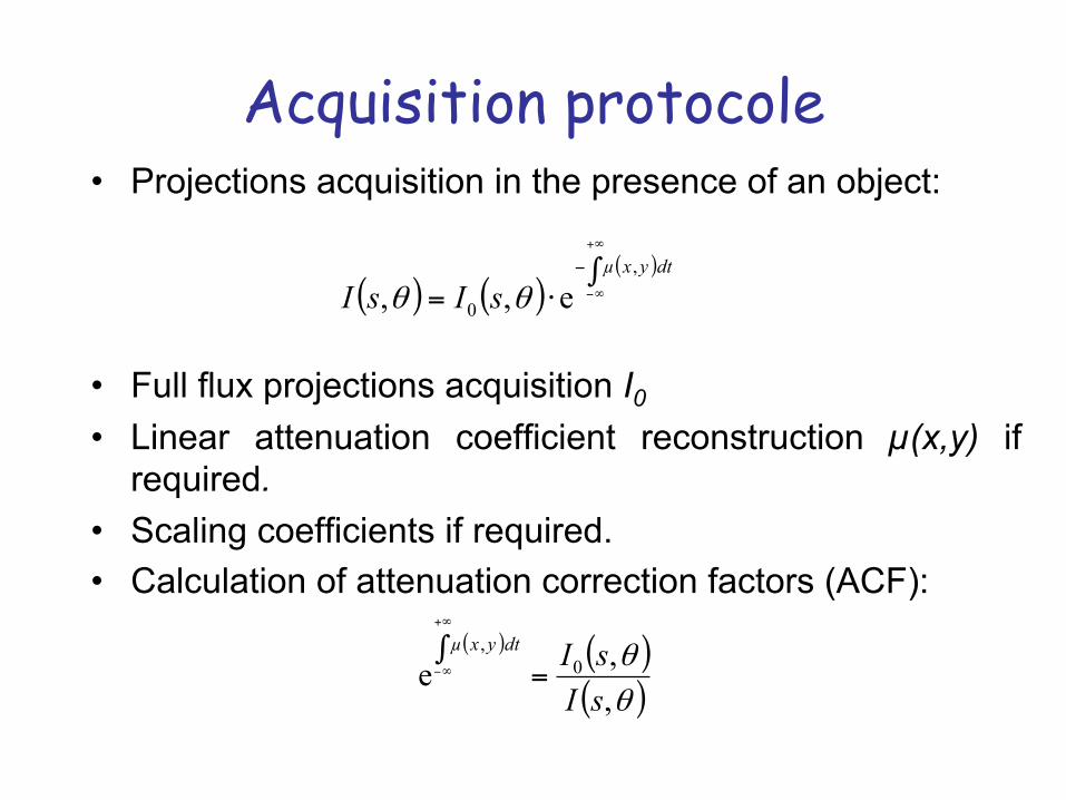
Acquisition protocole •  Projections acquisition in the presence of an object:

•  Full flux projections acquisition I0

•  Linear attenuation coefficient reconstruction µ(x,y) if required.

•  Scaling coefficients if required. •  Calculation of attenuation correction factors (ACF):

( ) ( )( )∫

⋅=

+∞

∞−

− dtyxµ

sIsI,

0 e,, θθ

( ) ( )( )θθ,,e 0

,

sIsIdtyxµ

=∫+∞

∞−

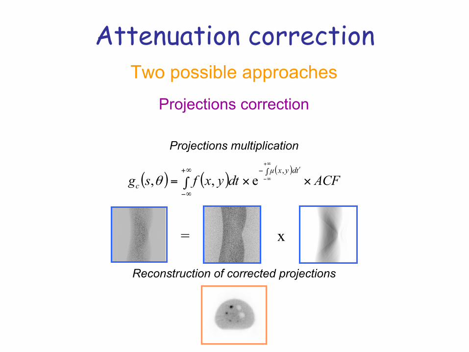
Attenuation correction Two possible approaches

Projections correction

Projections multiplication

Reconstruction of corrected projections

( ) ( )( )

ACFdtyxfsgtdyxµ

c ×∫ ×=∫ ʹ′−∞+

∞−

+∞

∞−,

e,,θ

= x

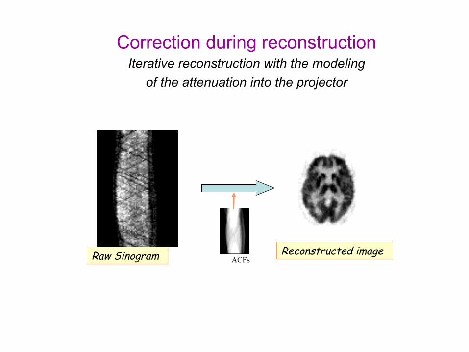
Correction during reconstruction Iterative reconstruction with the modeling

of the attenuation into the projector

Raw Sinogram Reconstructed image ACFs

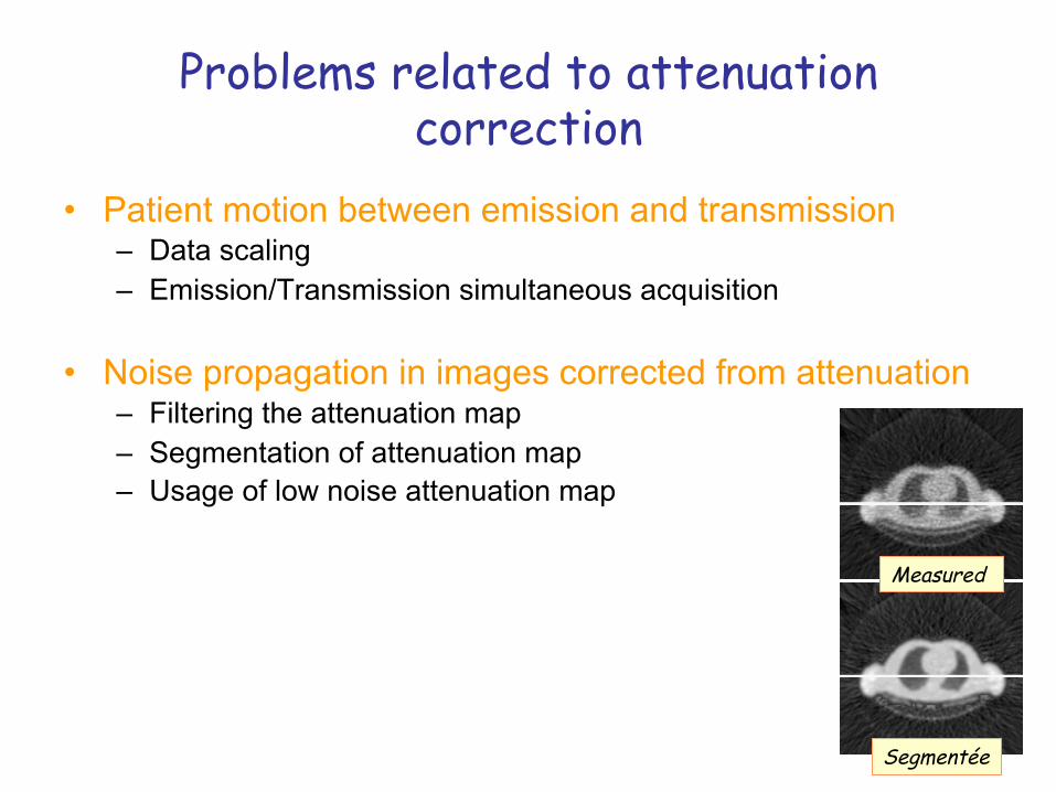
Problems related to attenuation correction

•  Patient motion between emission and transmission –  Data scaling –  Emission/Transmission simultaneous acquisition

•  Noise propagation in images corrected from attenuation –  Filtering the attenuation map –  Segmentation of attenuation map –  Usage of low noise attenuation map

Measured

Segmentée

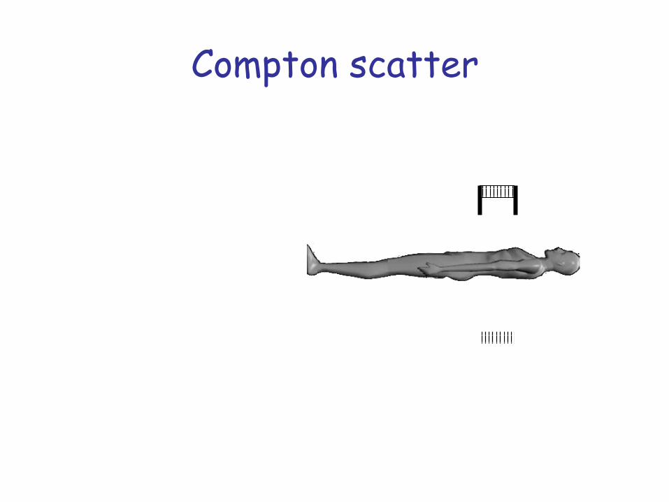
Compton scatter

Detection solid angle of unique photons

In patient Mispositioned coïncidence

Dans le cristal Détérioration de la résolution intrinsèque Rejet d’événements

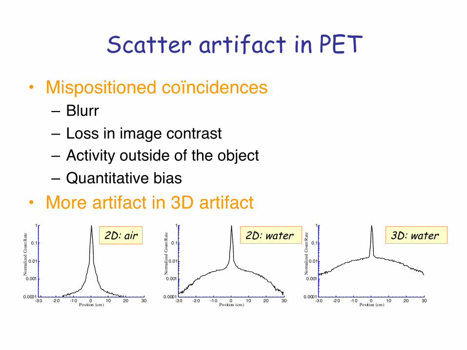
Scatter artifact in PET •  Mispositioned coïncidences

–  Blurr–  Loss in image contrast–  Activity outside of the object–  Quantitative bias

•  More artifact in 3D artifact

0.0001

0.001

0.01

0.1

1

-30 -20 -10 0 10 20 30

Nor

mal

ized

Cou

nt R

ate

Position (cm)

0.0001

0.001

0.01

0.1

1

-30 -20 -10 0 10 20 30

Nor

mal

ized

Cou

nt R

ate

Position (cm)

0.0001

0.001

0.01

0.1

1

-30 -20 -10 0 10 20 30N

orm

aliz

ed C

ount

Rat

ePosition (cm)

2D: air 2D: water 3D: water

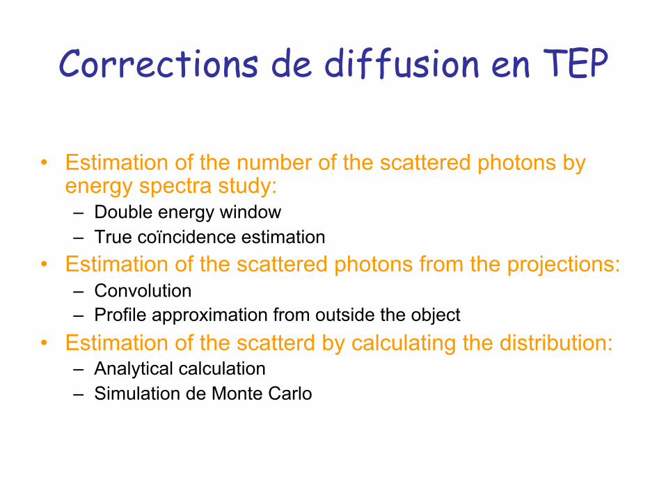
Corrections de diffusion en TEP

•  Estimation of the number of the scattered photons by energy spectra study: –  Double energy window –  True coïncidence estimation

•  Estimation of the scattered photons from the projections: –  Convolution –  Profile approximation from outside the object

•  Estimation of the scatterd by calculating the distribution: –  Analytical calculation –  Simulation de Monte Carlo

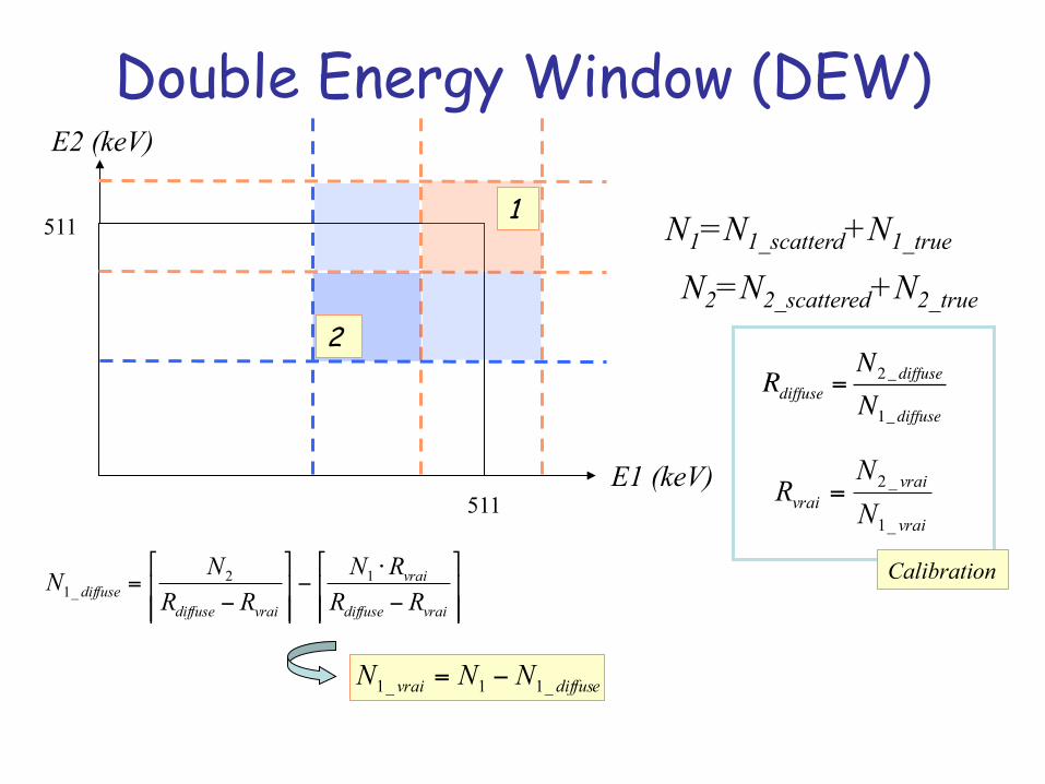
Double Energy Window (DEW)

E1 (keV)

E2 (keV)

511

511 1

2

N1=N1_scatterd+N1_true

N2=N2_scattered+N2_true

⎥⎥⎦

⎤

⎢⎢⎣

⎡

−⋅

−⎥⎥⎦

⎤

⎢⎢⎣

⎡

−=

vraidiffuse

vrai

vraidiffusediffuse RR

RNRR

NN 12_1

Rdiffuse =N2_diffuse

N1_diffuse

vrai

vraivrai N

NR

_1

_2=

Calibration

diffusevrai NNN _11_1 −=

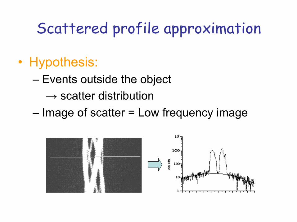
Scattered profile approximation

•  Hypothesis: – Events outside the object → scatter distribution –  Image of scatter = Low frequency image

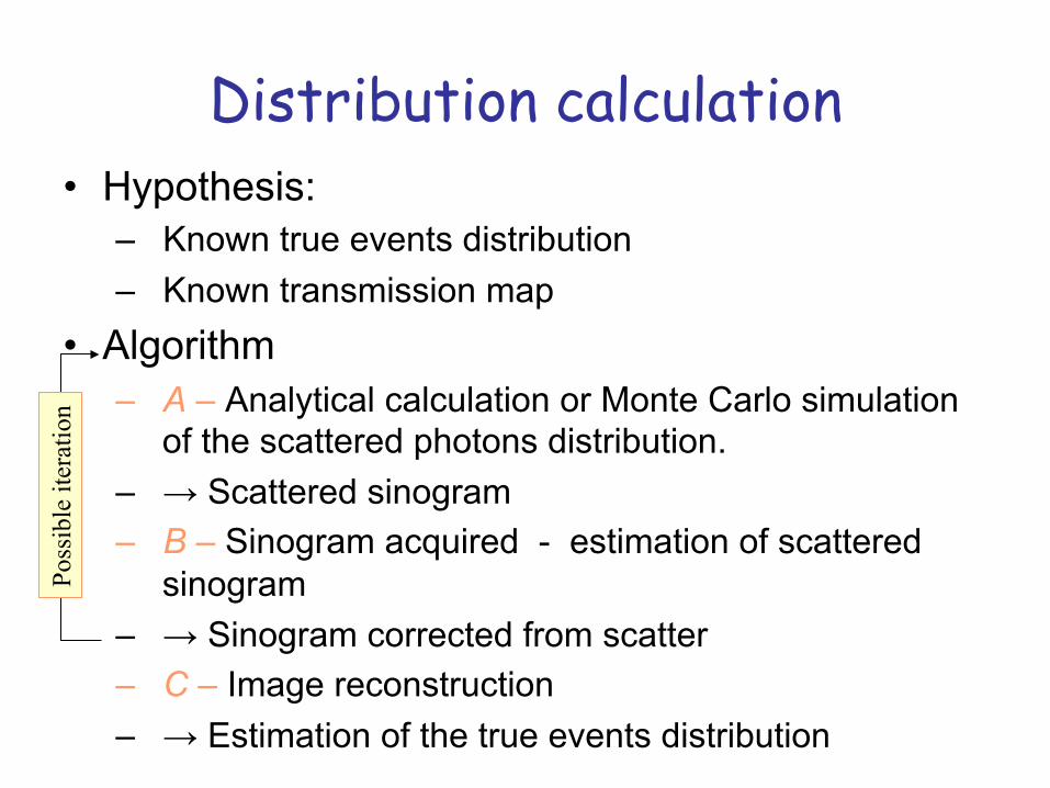
Distribution calculation •  Hypothesis:

–  Known true events distribution –  Known transmission map

•  Algorithm –  A – Analytical calculation or Monte Carlo simulation

of the scattered photons distribution. –  → Scattered sinogram –  B – Sinogram acquired - estimation of scattered

sinogram –  → Sinogram corrected from scatter –  C – Image reconstruction –  → Estimation of the true events distribution

Poss

ible

iter

atio

n

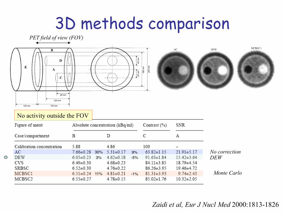
3D methods comparison

Zaidi et al, Eur J Nucl Med 2000:1813-1826

PET field of view (FOV)

No activity outside the FOV

No correction DEW

Monte Carlo

30% 9%3% -5%

11% -1%

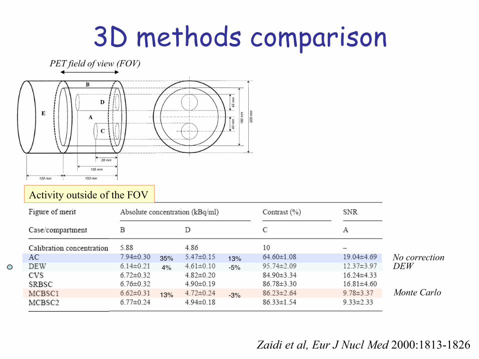
3D methods comparison

Zaidi et al, Eur J Nucl Med 2000:1813-1826

PET field of view (FOV)

Activity outside of the FOV

No correction DEW

Monte Carlo

35% 13%4% -5%

13% -3%

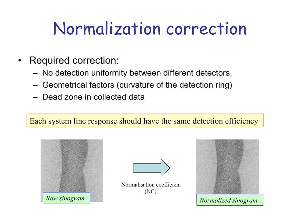
Normalization correction

•  Required correction: –  No detection uniformity between different detectors. –  Geometrical factors (curvature of the detection ring) –  Dead zone in collected data

Each system line response should have the same detection efficiency

Raw sinogram Normalized sinogram

Normalisation coefficient (NC)

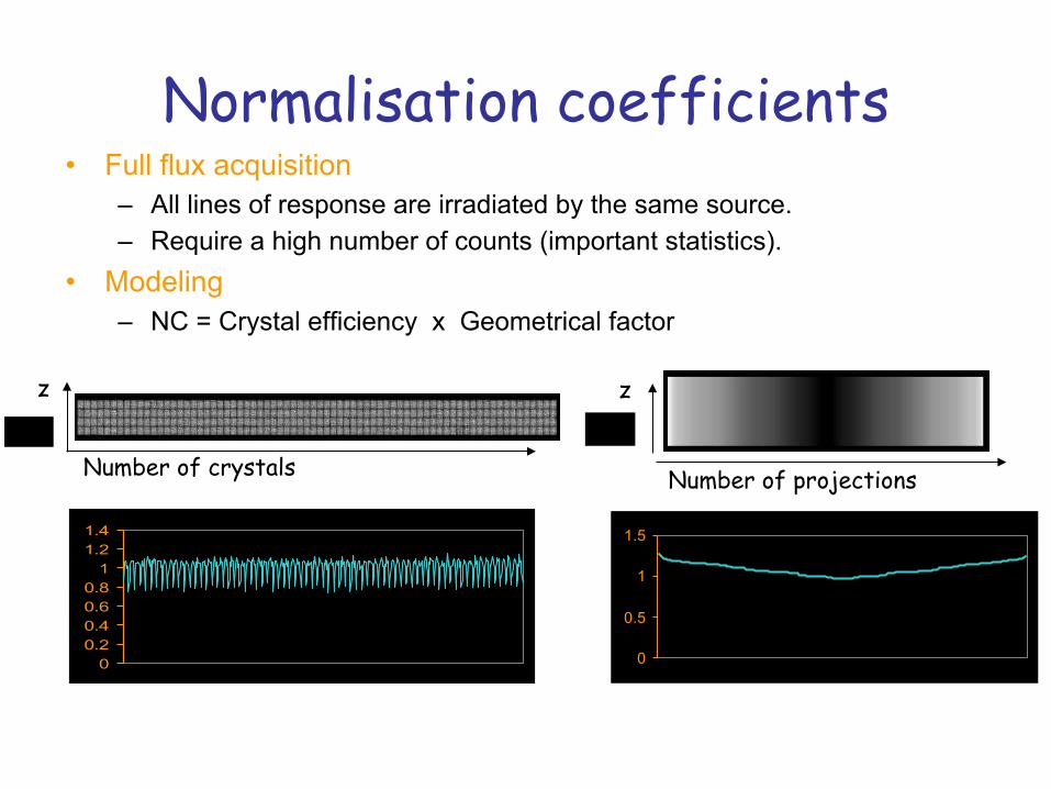
Normalisation coefficients •  Full flux acquisition

–  All lines of response are irradiated by the same source. –  Require a high number of counts (important statistics).

•  Modeling –  NC = Crystal efficiency x Geometrical factor

Number of crystals

z

00.20.40.60.81

1.21.4

Number of projections

z

0

0.5

1

1.5

)(xe)(xg

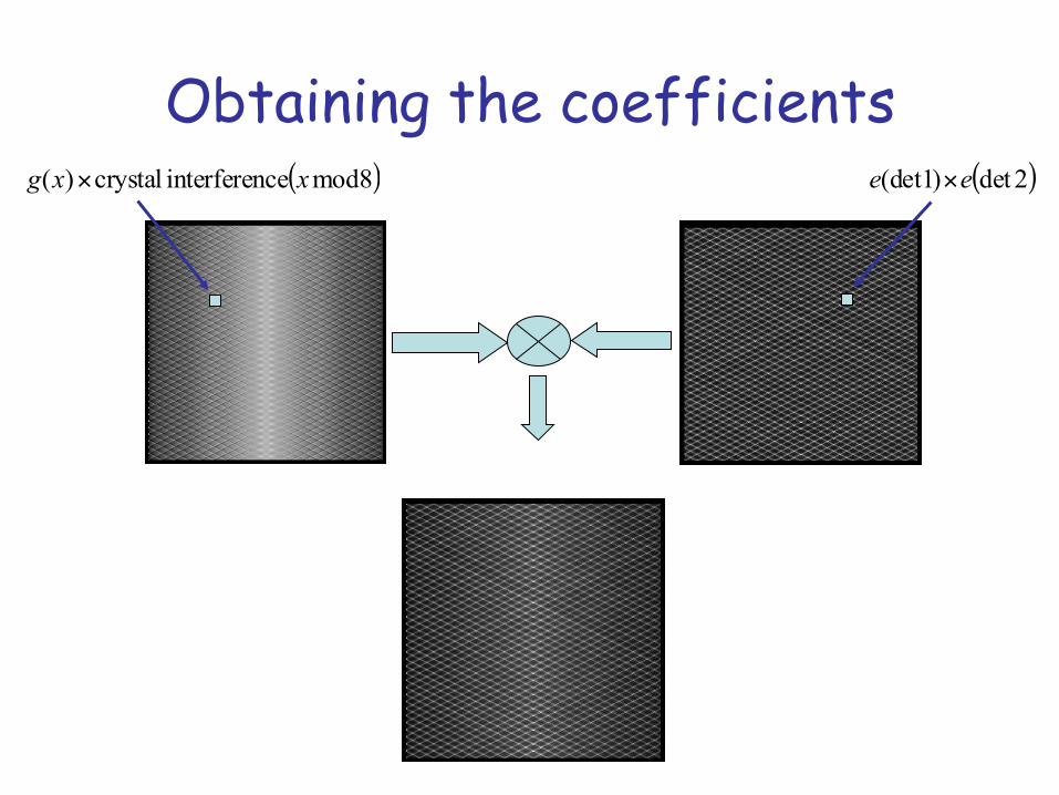
Obtaining the coefficients ( )8modceinterferen crystal)( xxg × ( )2det)1(det ee ×

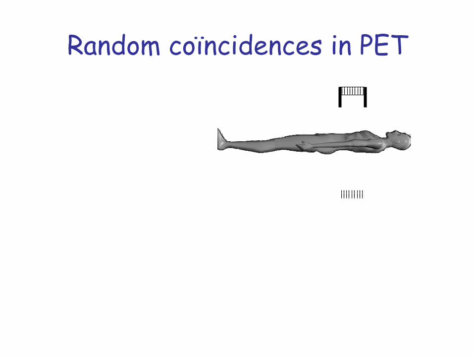
Random coïncidences in PET Detection solid angle of unique photon

jiij SSR τ2=•  Random coïncidences depend on:

–  Used time window •  Consequences of the random coïncidences:

–  Bad localisaton –  A quantitatif bias

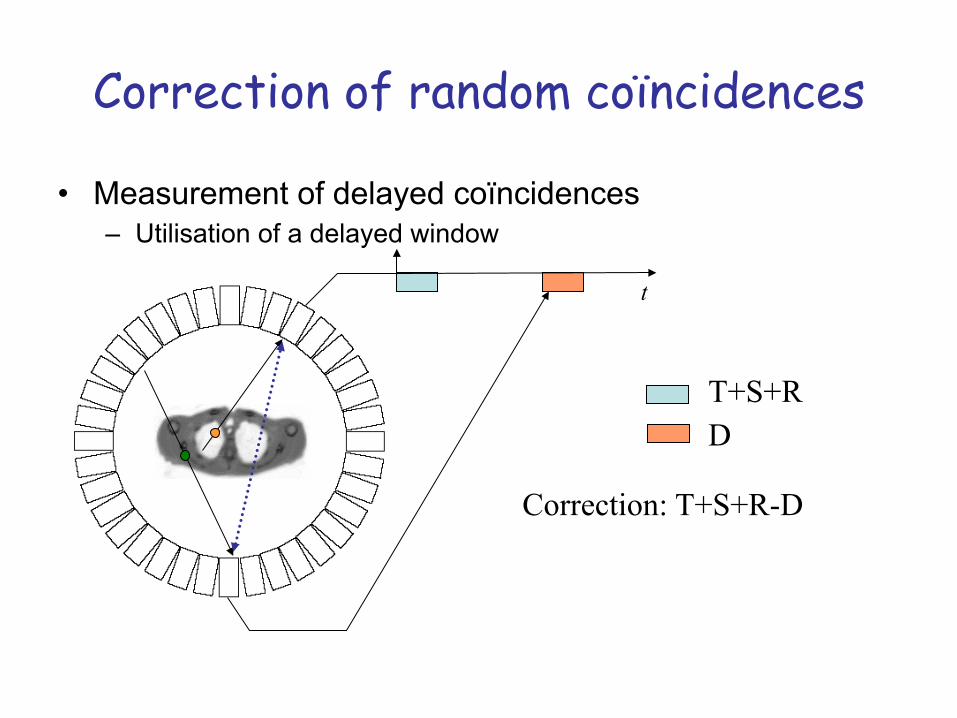
Correction of random coïncidences

•  Measurement of delayed coïncidences –  Utilisation of a delayed window

t

T+S+R D

Correction: T+S+R-D

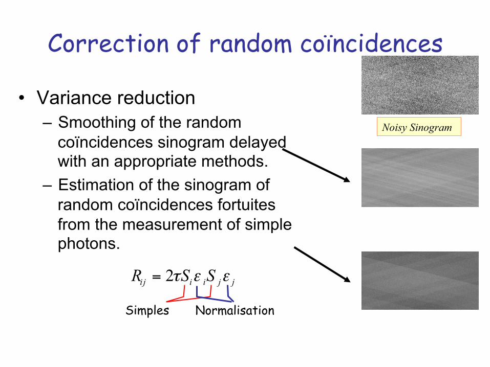
•  Variance reduction –  Smoothing of the random

coïncidences sinogram delayed with an appropriate methods.

–  Estimation of the sinogram of random coïncidences fortuites from the measurement of simple photons.

Noisy Sinogram

Rij = 2τSiε iS jε j

Simples Normalisation

Correction of random coïncidences

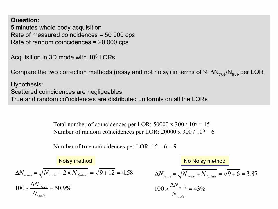
Question: 5 minutes whole body acquisition Rate of measured coïncidences = 50 000 cps Rate of random coïncidences = 20 000 cps Acquisition in 3D mode with 106 LORs Compare the two correction methods (noisy and not noisy) in terms of % ΔNtrue/Ntrue per LOR Hypothesis: Scattered coïncidences are negligeables True and random coïncidences are distributed uniformly on all the LORs

Total number of coïncidences per LOR: 50000 x 300 / 106 = 15 Number of random coïncidences per LOR: 20000 x 300 / 106 = 6 Number of true coïncidences per LOR: 15 – 6 = 9

%9,50100

58,41292

=Δ

×

=+=×+=Δ

vraie

vraie

fortuitvraievraie

NN

NNN ΔNvraie = Nvraie + N fortuit = 9+ 6 = 3,87

100× ΔNvraie

Nvraie

= 43%

Noisy method No Noisy method

Quality image estimation •  How to estimate the image quality?

–  Based on the concepts of: •  Sensibility: detection of true positives •  Specificity: détection de false positives •  → Receiver Operating Charactéristics: represents the

probability of detecting a true positive as function of detecting a false positive.

•  Difficult set up

•  Estimate the signal to noise ratio in the image: Noise Equivalent Count Rate

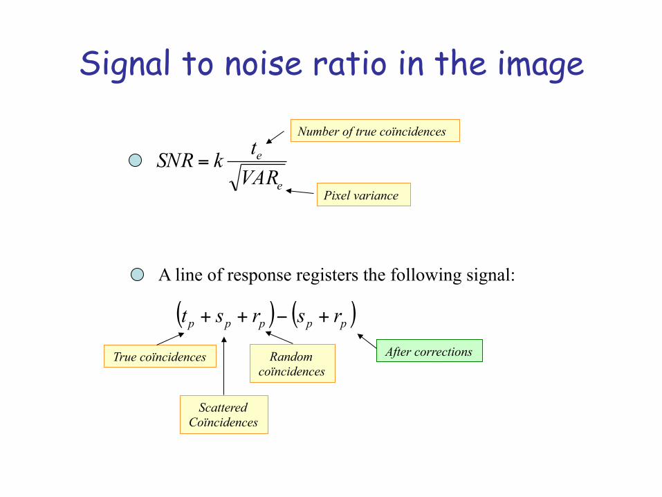
Signal to noise ratio in the image

e

e

VARtkSNR =

Number of true coïncidences

Pixel variance

A line of response registers the following signal:

( ) ( )ppppp rsrst +−++

True coïncidences Random coïncidences

Scattered Coïncidences

After corrections

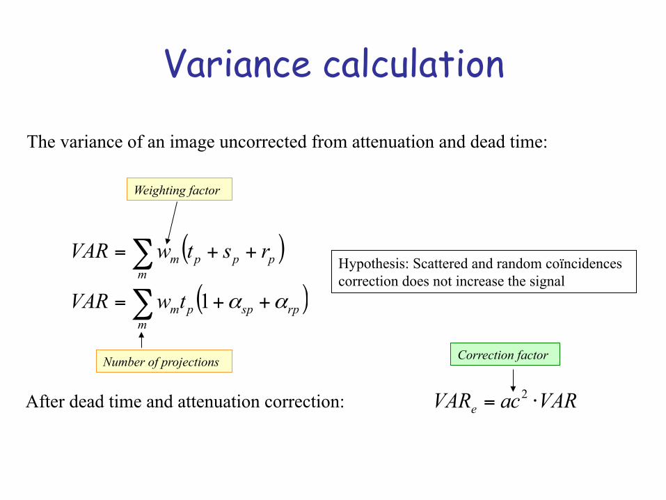
Variance calculation

The variance of an image uncorrected from attenuation and dead time:

( )

( )∑

∑

++=

++=

mrpsppm

mpppm

twVAR

rstwVAR

αα1

Number of projections

Weighting factor

Hypothesis: Scattered and random coïncidences correction does not increase the signal

After dead time and attenuation correction: VARacVARe ⋅= 2

Correction factor

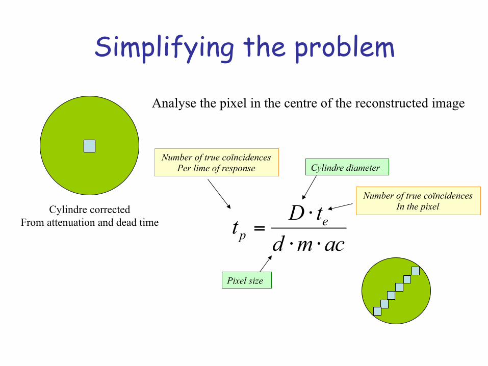
Simplifying the problem

Cylindre corrected From attenuation and dead time

Analyse the pixel in the centre of the reconstructed image

acmdtDt e

p ⋅⋅⋅

=

Number of true coïncidences Per lime of response

Number of true coïncidences In the pixel

Cylindre diameter

Pixel size

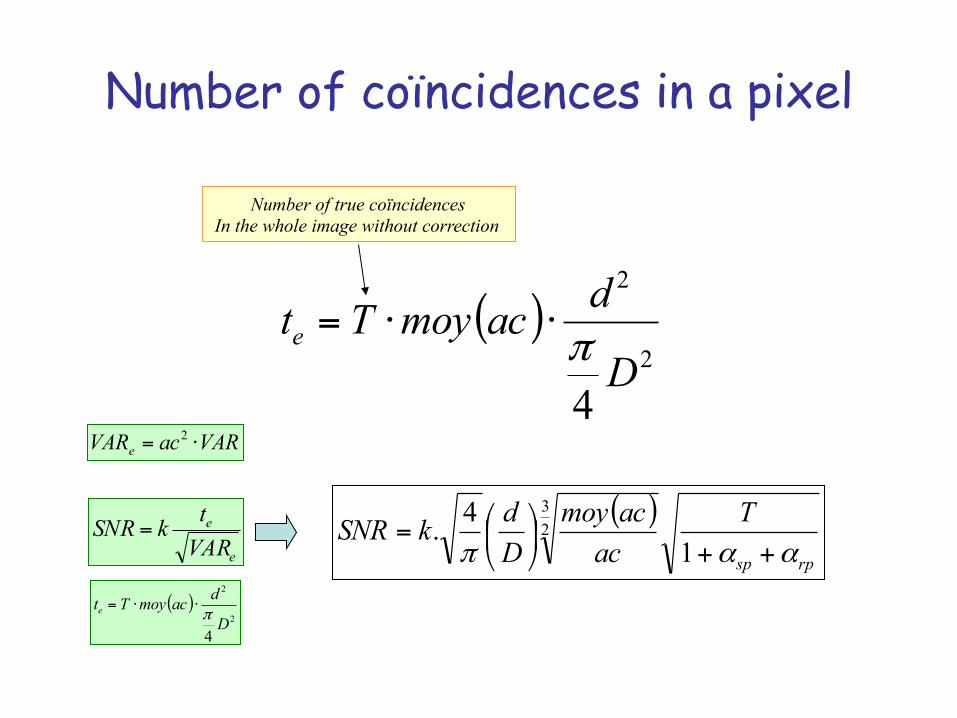
Number of coïncidences in a pixel

( )2

2

4D

dacmoyTte π⋅⋅=

e

e

VARtkSNR = ( )

rpsp

Tacacmoy

DdkSNR

ααπ ++⎟⎠

⎞⎜⎝

⎛=1

4. 23

VARacVARe ⋅= 2

( )2

2

4D

dacmoyTte π⋅⋅=

Number of true coïncidences In the whole image without correction

Noise Equivalent Count ( ) NECacacmoy

DdkSNR 2

34. ⎟⎠

⎞⎜⎝

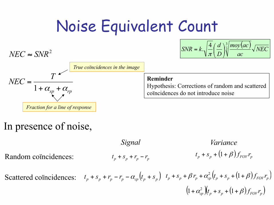
⎛=π2SNRNEC ≈

rpsp

TNECαα ++

=1

Fraction for a line of response

True coïncidences in the image

Reminder Hypothesis: Corrections of random and scattered coïncidences do not introduce noise

In presence of noise,

Random coïncidences: pppp rrst −++

Signal Variance

Scattered coïncidences: ( )( )pFOVppcpppp rfstrst βαβ ++++++ 12( )ppcppppp strrst +−−++ α

( ) pFOVpp rfst β+++ 1

( ) ( )( )pFOVppcp rfst βα ++++ 11 2

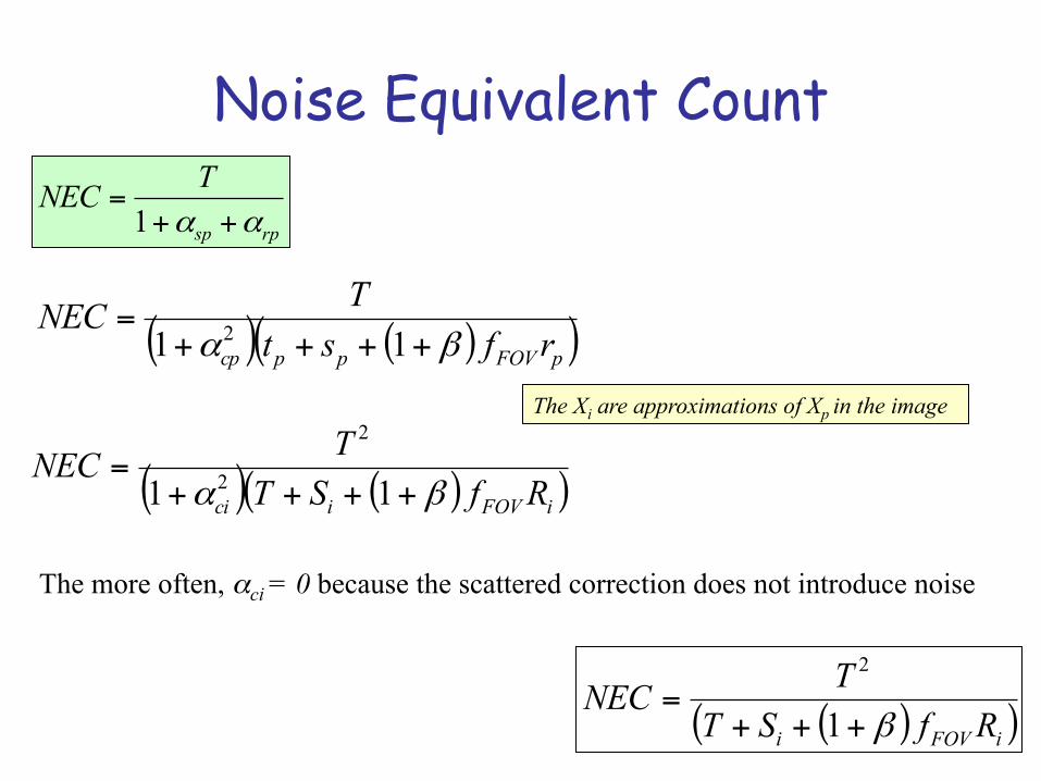
Noise Equivalent Count

rpsp

TNECαα ++

=1

( ) ( )( )pFOVppcp rfstTNEC

βα ++++=

11 2

( ) ( )( )iFOVici RfSTTNEC

βα ++++=

11 2

2The Xi are approximations of Xp in the image

The more often, αci = 0 because the scattered correction does not introduce noise

( )( )iFOVi RfSTTNECβ+++

=1

2

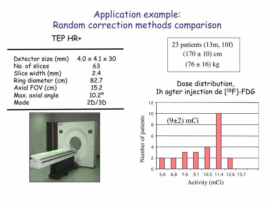
Application example: Random correction methods comparison TEP HR+

Detector size (mm) No. of slices Slice width (mm) Ring diameter (cm) Axial FOV (cm) Max. axial angle Mode

4.0 x 4.1 x 30 63 2.4

82.7 15.2 10.2º

2D/3D

23 patients (13m, 10f) (170 ± 10) cm(76 ± 16) kg

Dose distribution, 1h agter injection de [18F]-FDG

0

2

4

6

8

10

12

5.6 6.8 7.9 9.1 10.3 11.4 12.6 13.7

(9±2) mCi

Activity (mCi)

Num

ber o

f pat

ient

s

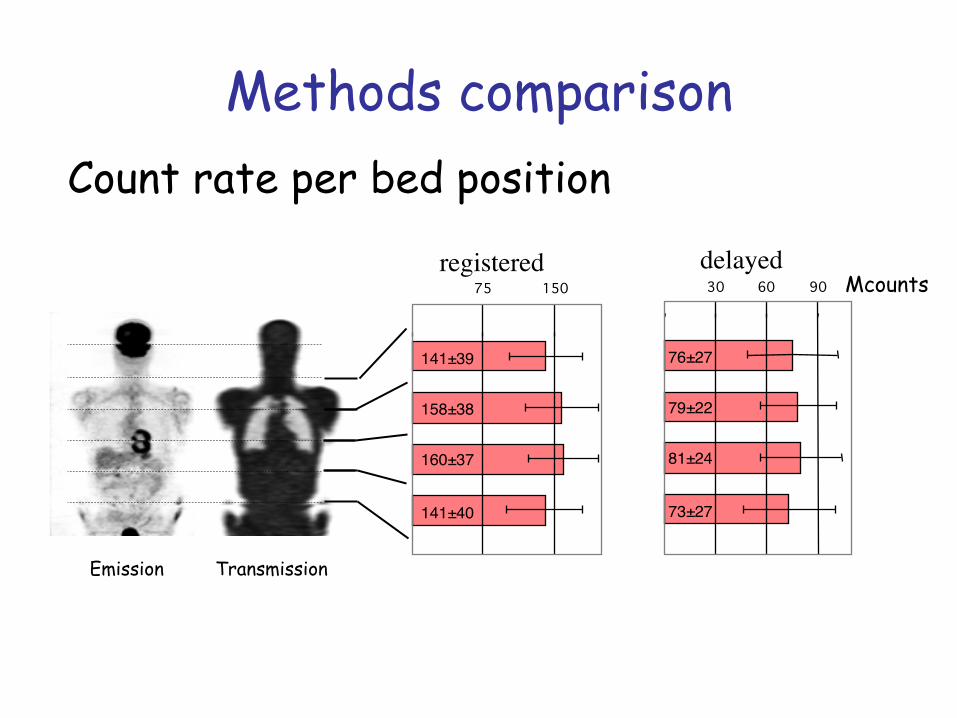
Methods comparison Count rate per bed position

Transmission

75 150 30 60 90 Mcounts registered delayed

141±39

158±38

160±37

141±40

76±27

79±22

81±24

73±27

Emission

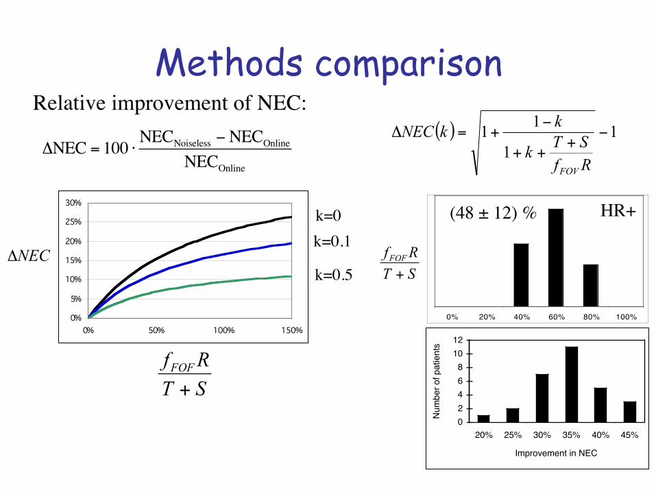
Methods comparison Relative improvement of NEC:

0%

5%

10%

15%

20%

25%

30%

0% 50% 100% 150%

k=0k=0.1

k=0.5

ΔNEC = 100 ⋅ NECNoiseless −NECOnlineNECOnline

( ) 11

11 −+

++

−+=Δ

RfSTk

kkNEC

FOV

NECΔ

0% 20% 40% 60% 80% 100%

(48 ± 12) %

STRfFOF

+

STRfFOF

+

HR+

02468

1012

20% 25% 30% 35% 40% 45%

Improvement in NEC

Num

ber o

f pat

ient

s

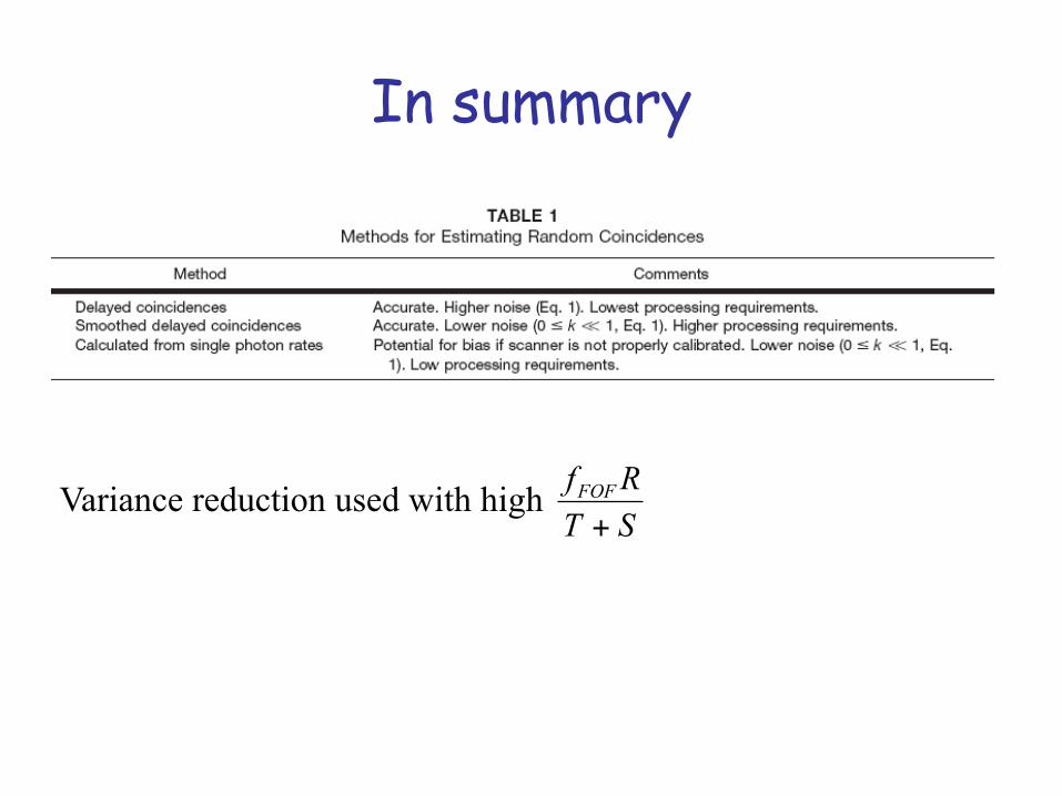
In summary

Variance reduction used with high STRfFOF

+

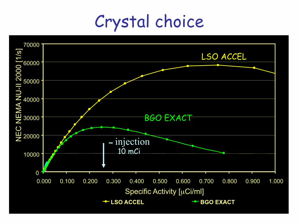
Crystal choice

1.000

NE

C N

EM

A N

U-II

200

0 [1

/s]

0

10000

20000

30000

40000

50000

60000

70000

0.000 0.100 0.200 0.300 0.400 0.500 0.600 0.700 0.800 0.900 Specific Activity [µCi/ml]

LSO ACCEL BGO EXACT

≈ injection 10 mCi

BGO EXACT

LSO ACCEL