Job Duration and the Informal Sector in Brazil

Gabriel Ulyssea Dimitri Szermanulyssea@ipea.gov.br dimitrijoe@ipea.gov.br

Instituto de Pesquisa economica AplicadaAv. Presidente Antonio Carlos, 51, 14o andar

Centro, 20020-010Rio de Janeiro, RJ

24th July 2006

Abstract

We use data from the Monthly Employment Survey [Pesquisa Mensaldo Emprego (PME)] to estimate the determinants of job duration in theformal and informal sectors of the Brazilian labor market. We analyzeworkers’ mobility patterns using reduced-form duration models, which aretraditionally used in unemployment analysis. The technics used involveboth non-parametric and parametric tools. Our main findings are thattransitions out of the formal and informal labor market are governed bydifferent patterns. While schooling and age are positively associated withjob duration in the formal sector, the opposite is true for the informalsector. Also, we find indications of the existence of an “informality trap”,as the hazard rates out of informal job decline monotonically and quiterapidly over time. This suggest that if the worker does not move outof informal employment within, say, the first 3-6 months, he is likely toexperience a long informal spell.

1

Introduction

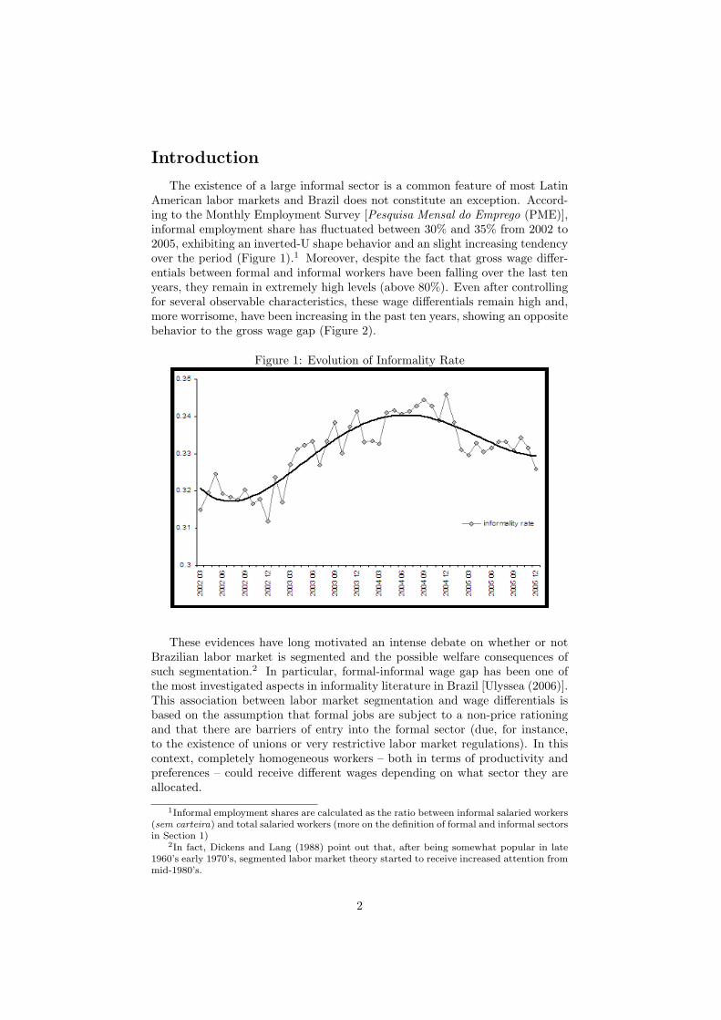
The existence of a large informal sector is a common feature of most LatinAmerican labor markets and Brazil does not constitute an exception. Accord-ing to the Monthly Employment Survey [Pesquisa Mensal do Emprego (PME)],informal employment share has fluctuated between 30% and 35% from 2002 to2005, exhibiting an inverted-U shape behavior and an slight increasing tendencyover the period (Figure 1).1 Moreover, despite the fact that gross wage differ-entials between formal and informal workers have been falling over the last tenyears, they remain in extremely high levels (above 80%). Even after controllingfor several observable characteristics, these wage differentials remain high and,more worrisome, have been increasing in the past ten years, showing an oppositebehavior to the gross wage gap (Figure 2).

Figure 1: Evolution of Informality Rate

These evidences have long motivated an intense debate on whether or notBrazilian labor market is segmented and the possible welfare consequences ofsuch segmentation.2 In particular, formal-informal wage gap has been one ofthe most investigated aspects in informality literature in Brazil [Ulyssea (2006)].This association between labor market segmentation and wage differentials isbased on the assumption that formal jobs are subject to a non-price rationingand that there are barriers of entry into the formal sector (due, for instance,to the existence of unions or very restrictive labor market regulations). In thiscontext, completely homogeneous workers – both in terms of productivity andpreferences – could receive different wages depending on what sector they areallocated.

1Informal employment shares are calculated as the ratio between informal salaried workers(sem carteira) and total salaried workers (more on the definition of formal and informal sectorsin Section 1)

2In fact, Dickens and Lang (1988) point out that, after being somewhat popular in late1960’s early 1970’s, segmented labor market theory started to receive increased attention frommid-1980’s.

2

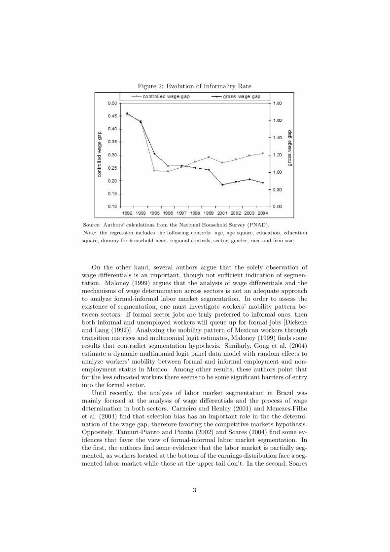
Figure 2: Evolution of Informality Rate

Source: Authors’ calculations from the National Household Survey (PNAD).

Note: the regression includes the following controls: age, age square, education, education

square, dummy for household head, regional controls, sector, gender, race and firm size.

On the other hand, several authors argue that the solely observation ofwage differentials is an important, though not sufficient indication of segmen-tation. Maloney (1999) argues that the analysis of wage differentials and themechanisms of wage determination across sectors is not an adequate approachto analyze formal-informal labor market segmentation. In order to assess theexistence of segmentation, one must investigate workers’ mobility pattern be-tween sectors. If formal sector jobs are truly preferred to informal ones, thenboth informal and unemployed workers will queue up for formal jobs [Dickensand Lang (1992)]. Analyzing the mobility pattern of Mexican workers throughtransition matrices and multinomial logit estimates, Maloney (1999) finds someresults that contradict segmentation hypothesis. Similarly, Gong et al. (2004)estimate a dynamic multinomial logit panel data model with random effects toanalyze workers’ mobility between formal and informal employment and non-employment status in Mexico. Among other results, these authors point thatfor the less educated workers there seems to be some significant barriers of entryinto the formal sector.

Until recently, the analysis of labor market segmentation in Brazil wasmainly focused at the analysis of wage differentials and the process of wagedetermination in both sectors. Carneiro and Henley (2001) and Menezes-Filhoet al. (2004) find that selection bias has an important role in the the determi-nation of the wage gap, therefore favoring the competitive markets hypothesis.Oppositely, Tannuri-Pianto and Pianto (2002) and Soares (2004) find some ev-idences that favor the view of formal-informal labor market segmentation. Inthe first, the authors find some evidence that the labor market is partially seg-mented, as workers located at the bottom of the earnings distribution face a seg-mented labor market while those at the upper tail don’t. In the second, Soares

3

(2004) also analyzes labor market segmentation trough the lens of wage deter-mination and wage differentials literature (he estimates a endogenous switchingmodel). However, he employs a job queue approach and, therefore, his work isalso related to the job mobility literature.

An important early exception in the literature relative to labor market seg-mentation in Brazil is the work of Barros et al. (1990), which investigates themobility of formal and informal employees in the metropolitan region of SaoPaulo.3 These authors find high mobility rates between both sectors, estimatingthat nearly 50% of informal workers in any given year will be employed in formaljobs in the following year. Therefore, they conclude that the consequences ofinformality are only relevant in the short term and don’t have any great impacton long term wage distribution. More recently, Curi and Menezes-Filho (2006)have carefully characterized labor market evolution in the 1980’s and 1990’s andanalyzed the determinants of employment transition in Brazil. Moreover, theseauthors investigate average conditional wage changes associated to labor markettransitions, exploiting the panel structure of the PME. They find that transi-tions from formality to informality and the other way around are associated tosmall wage decreases and increases, respectively (around 7%). Therefore, theyconclude that there is some labor market segmentation in Brazil, but due toits reduce magnitude, it is likely to have minor effects on wage distribution andworkers’ welfare.

The objective of this paper is twofold. First, we aim to contribute to thecharacterization of Brazilian labor market, by providing some stylized factsrelative to formal and informal employment spells, exit rates to other statesand how these vary over time (duration dependence). By doing that, we alsotackle a fundamental component of informality rate, namely, the duration ofinformality. The idea here is that, analogously to unemployment analysis, forany given flow of entry into the informal sector (let us name it the incidencerate), the higher informality duration the higher the observed informality rate.Second, and perhaps more importantly, we aim to contribute to the debateon the existence and possible consequences of formal-informal labor marketsegmentation in Brazil.

We analyze workers’ mobility patterns through duration models, which aretraditionally used in unemployment analysis.4 We estimate reduced-form equa-tions trying to identify the determinants of job duration. Given our objectives,special attention is given to differences between formal and informal job sectors.Although there is a growing literature in employment duration analysis [see,for instance, Lindeboom and Theeuwes (1991) and Christofides and McKenna(1996)], there is no piece of literature on employment duration in Brazil usingsuch methods5.

We find significantly different patterns for transitions out of the formal andinformal sectors. While schooling and age are positively associated with jobduration in the formal sector, the opposite is true for the informal sector. This

3Is worth mentioning the work of Ancora et al. (1997), which doesn’t directly address theissue of labor market segmentation, but also analyzes workers mobility in both sectors.

4For a comprehensive survey of duration models and some applications to unemploymentduration analysis, see Van den Berg (2001). For an unemployment duration analysis in Brazil,see Menezes-Filho and Picchetti (2000).

5There is, however, a related literature in job turnover in Brazil (for a survey, see Gonzaga(2003)). These works encompass job duration but do not take into account censoring andrelated features of duration data.

4

reinforces the view that informal jobs are of inferior quality, because the moreable workers, with a broader menu of job options, are choosing formal jobs.Our findings also point to the existence of an “informality trap”, as the hazardrates out of informal job decline monotonically and quite rapidly over time. Thissuggest that if the worker does not move out of informal employment within, say,the first 3-6 months, he is likely to experience a long informal spell. Moreover,once we disentangle the risks out of informal and informal sectors, we find thatinformal-formal transitions are substantially less likely to happen than the otherway around.

The remaining of the paper is organized as follows. Section 1 provides in-formation on our dataset. In Section 2 we explore data using non-parametrictools. In Section 3 we present out empirical models and discuss estimation re-sults. Finally, Section 4 we make a more broad discussion of our results andoutline further extensions of this work.

1 Data description

This paper uses panel data from the Pesquisa Mensal de Emprego (PME) forthe period from March 2002 to December 20056. In 2002 the PME went throughmajor changes, among which was the inclusion in the survey questionnaire ofretrospective questions about job duration. It is often argued that retrospectivequestions are likely to be contaminated with recall errors, specially for eventsthat happened a long time in the past. We present a detailed discussion aboutthe quality of this information in the Appendix.

To construct our sample, we use information from the first four interviewsof each individual7. We select only individuals who report to be employed inthe private sector in at least one interview8. This means, for example, that anindividual in self-employment during the first two interviews and unemployedin the last two interviews is excluded from the sample. To avoid inconsistenciesin the job duration measure, we exclude individuals holding more than one job.Also, we restrict the sample to individuals aged 15 to 65 years old in the fourinterviews. Details on the effects of selection rules on sample size and samplecomposition are presented in the Appendix.

Throughout the paper, we consider only one job spell per individual. Thatis, if an individual changes jobs, we ignore the spell of the second job. Thereis a caveat in our definition of a job spell. The PME does not ask respondentsif their current job is the same as the job they held in the preceding interview.What is actually observed is the individual’s job duration and occupationalstatus. Therefore, in analyzing transitions, we take the occupational status asan individual’s job. As a result, job changes within the same occupational statusare ignored in the sense that they are not regarded as transitions. This caveat

6The PME is a monthly household survey conducted by the Instituto Brasileiro de Ge-ografia e Estatıstica (IBGE). It is representative of the six major metropolitan areas in Brazil,namely Belo Horizonte, Porto Alegre, Recife, Rio de Janeiro, Salvador and Sao Paulo. Thesurvey structure is similar to that of the US Current Population Surveys (CPS): selectedhouseholds are interviewed once a month for four months, leave the sample and return eightmonths later for another four months of interviews.

7That we do not use information from all the eight interviews is due to problems withmatching the individuals across the fourth and fifth interviews.

8Domestic work was not considered to be in the private sector.

5

is likely to introduce a positive bias in job duration figures presented in thispaper.

Table 1 shows descriptive statistics for the sample. The two possible initialoccupational status are formal and informal9. Formal workers are those whosejob is regulated by a formal labor contract (carteira assinada), and informalworkers do not posses this sort of contract. One third of the sample consistsof informal workers. Moreover, the last line of Table 1 shows that nearly twothirds of the job spells are right-censored.

Table 2 shows the patterns of transitions between the initial state (infor-mal or formal job) and the various possible destinations. The destinationsare broadly divided into “employment” (including self-employment) and “non-employment”. Note that any transition within the same occupational status isregarded as right-censored so the cells informal-informal and formal-formal givethe same numbers as the appropriate cells in the last line of Table 1. We cansee that transitions informal-formal are much more likely than formal-informaltransitions. These figures alone could suggest absence of market segmentation(Maloney (1999)). However, as outlined in Table 1, formal and informal work-ers are quite different in their characteristics, and so a more careful analysis iscalled for.

9Therefore any informal-informal or formal-formal movement is treated as right censored.

6

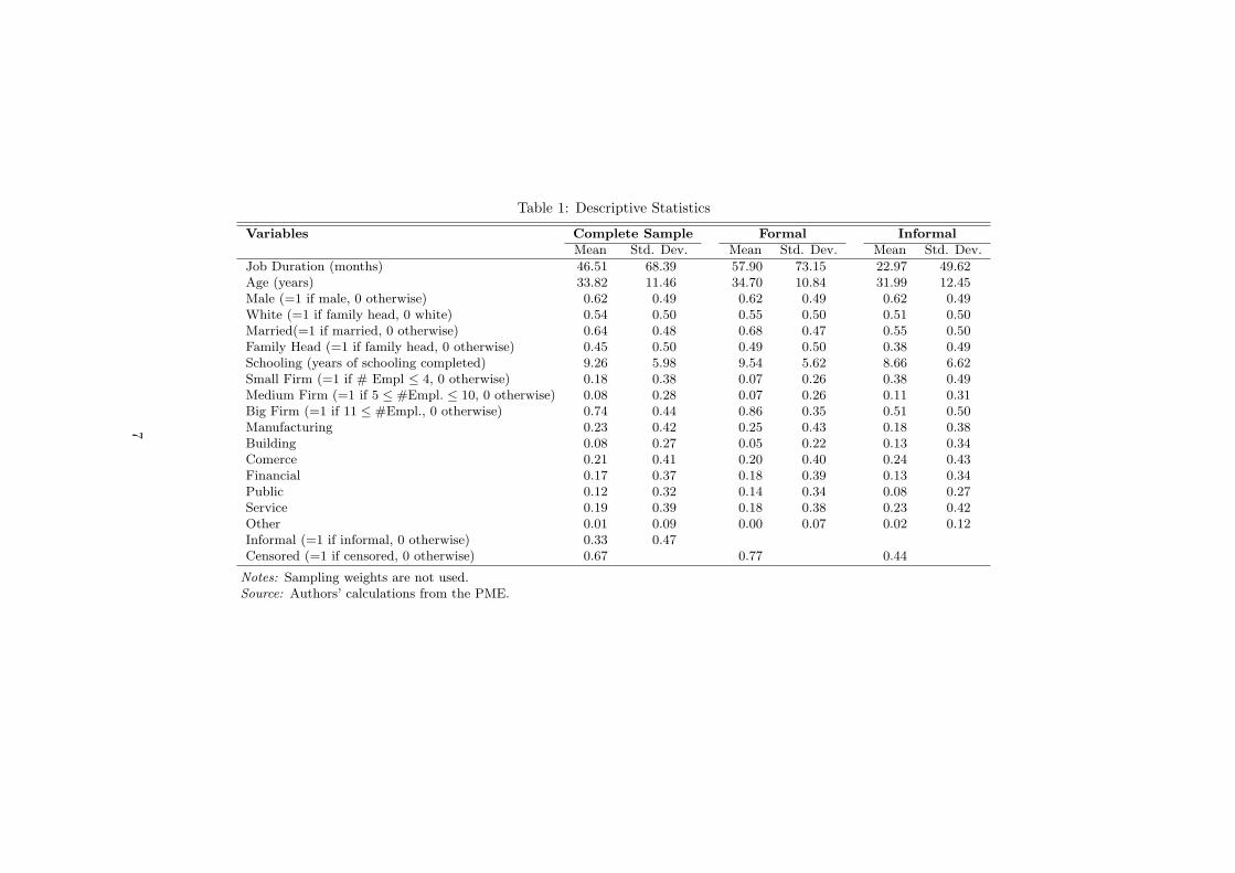
Table 1: Descriptive Statistics

Variables Complete Sample Formal InformalMean Std. Dev. Mean Std. Dev. Mean Std. Dev.

Job Duration (months) 46.51 68.39 57.90 73.15 22.97 49.62Age (years) 33.82 11.46 34.70 10.84 31.99 12.45Male (=1 if male, 0 otherwise) 0.62 0.49 0.62 0.49 0.62 0.49White (=1 if family head, 0 white) 0.54 0.50 0.55 0.50 0.51 0.50Married(=1 if married, 0 otherwise) 0.64 0.48 0.68 0.47 0.55 0.50Family Head (=1 if family head, 0 otherwise) 0.45 0.50 0.49 0.50 0.38 0.49Schooling (years of schooling completed) 9.26 5.98 9.54 5.62 8.66 6.62Small Firm (=1 if # Empl ≤ 4, 0 otherwise) 0.18 0.38 0.07 0.26 0.38 0.49Medium Firm (=1 if 5 ≤ #Empl. ≤ 10, 0 otherwise) 0.08 0.28 0.07 0.26 0.11 0.31Big Firm (=1 if 11 ≤ #Empl., 0 otherwise) 0.74 0.44 0.86 0.35 0.51 0.50Manufacturing 0.23 0.42 0.25 0.43 0.18 0.38Building 0.08 0.27 0.05 0.22 0.13 0.34Comerce 0.21 0.41 0.20 0.40 0.24 0.43Financial 0.17 0.37 0.18 0.39 0.13 0.34Public 0.12 0.32 0.14 0.34 0.08 0.27Service 0.19 0.39 0.18 0.38 0.23 0.42Other 0.01 0.09 0.00 0.07 0.02 0.12Informal (=1 if informal, 0 otherwise) 0.33 0.47Censored (=1 if censored, 0 otherwise) 0.67 0.77 0.44

Notes: Sampling weights are not used.Source: Authors’ calculations from the PME.

7

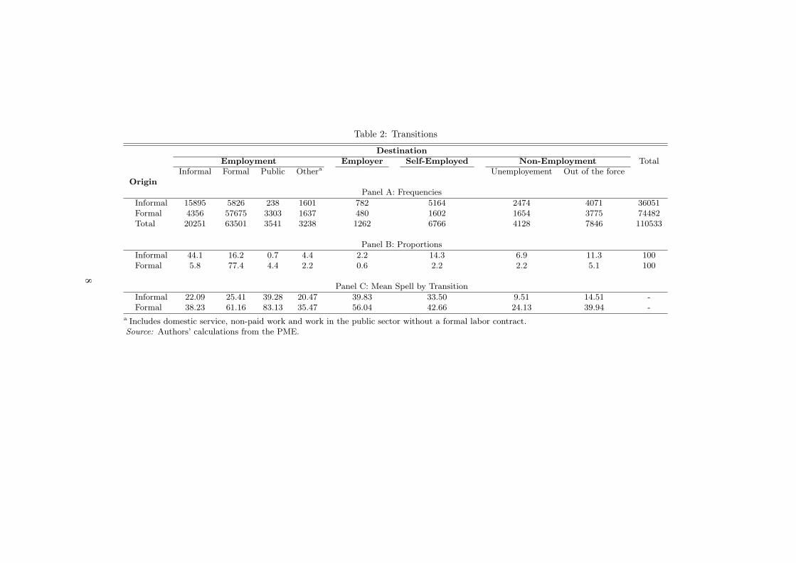
Table 2: Transitions

DestinationEmployment Employer Self-Employed Non-Employment Total

Informal Formal Public Othera Unemployement Out of the forceOrigin

Panel A: Frequencies

Informal 15895 5826 238 1601 782 5164 2474 4071 36051Formal 4356 57675 3303 1637 480 1602 1654 3775 74482Total 20251 63501 3541 3238 1262 6766 4128 7846 110533

Panel B: Proportions

Informal 44.1 16.2 0.7 4.4 2.2 14.3 6.9 11.3 100Formal 5.8 77.4 4.4 2.2 0.6 2.2 2.2 5.1 100

Panel C: Mean Spell by Transition

Informal 22.09 25.41 39.28 20.47 39.83 33.50 9.51 14.51 -Formal 38.23 61.16 83.13 35.47 56.04 42.66 24.13 39.94 -

a Includes domestic service, non-paid work and work in the public sector without a formal labor contract.Source: Authors’ calculations from the PME.

8

2 Nonparametric Analysis of Job Duration

Nonparametric methods impose minimal assumptions to the data, whichmakes their use a natural start point for any duration study. The analysis hereis essentially exploratory, in the sense that it is not meant to establish causalrelationships nor to quantify the effects of one variable on other variables.

One can analyze the distribution of a random variable from many perspec-tives. For instance, both the density function and the cumulative distributionfunction give full descriptions of a random variable. The choice of which func-tion to use depends on the feature of the distribution which is to me modelled.Economists are often interested in duration dependence. As a result, the haz-ard function is typically used by the economic literature in duration analysis,specially in parametric models. In nonparametric analysis, however, plots ofthe empirical hazard function are difficult to interpret as they lack smoothness.Plots of the integrated hazard are more convenient, and so are plots of thesurvivor function for their direct interpretation. This section uses both of thisfunctions to give a description of the data.

To obtain nonparametric estimates of the survivor and cumulative hazardfunctions, we use product-limit estimators10. Plots of these fuctions for formaland informal sectors are presented in Figures 3a and 3b. As can be seen, sharpcontrasts are revealed. While the survivor function for jobs in the informal sectorhas a convex shape, the plot for formal jobs seems to be linear in duration. Inturn, plots of the cumulative hazard display a concave shape for informal jobs,and is linear for formal jobs. This is an indication (see Kiefer (1988)) of negativeduration dependence in the first case, and no duration dependence at all in thelatter. Second, there is a considerable distance between the curves. For instance,the probability of surviving in a formal job after 100 months is nearly 75%, whilethe survivor probability for the informal counterpart is only 25%. This reflectsthe differences between average duration for formal and informal jobs, which isline with the common view that formal lasts for longer.

Since this analysis is not controlling for any variables possibly correlatedwith job sector, it could be that the informal-formal differences are due to otherfactors. For example, since it is natural to expect that firm size is negativelycorrelated with job informality, it could be that the above mentioned differencesare due to firm size. In fact, Figure 6a (see the Appendix) shows that, for anyduration, jobs in small firms have less probability of surviving than jobs inbigger firms. However, we make separate plots in an attempt to control forjob sector – shown Figures 6b and 6c, also in the Appendix –, and note thatthe differences depicted in Figure 6a practically vanish. The same is true forother job characteristics and for demographic variables. Other selected plotsare shown in the Appendix11.

10These are the Kaplan-Meier and Nelson-Aalen estimators for the survivor and cumulativehazard, respectively. See, for example, Kiefer (1988).

11Plots controlling for firm sector, geographic region, sex, cohort, schooling, race, andstatus in the household are available from the authors on request.

9

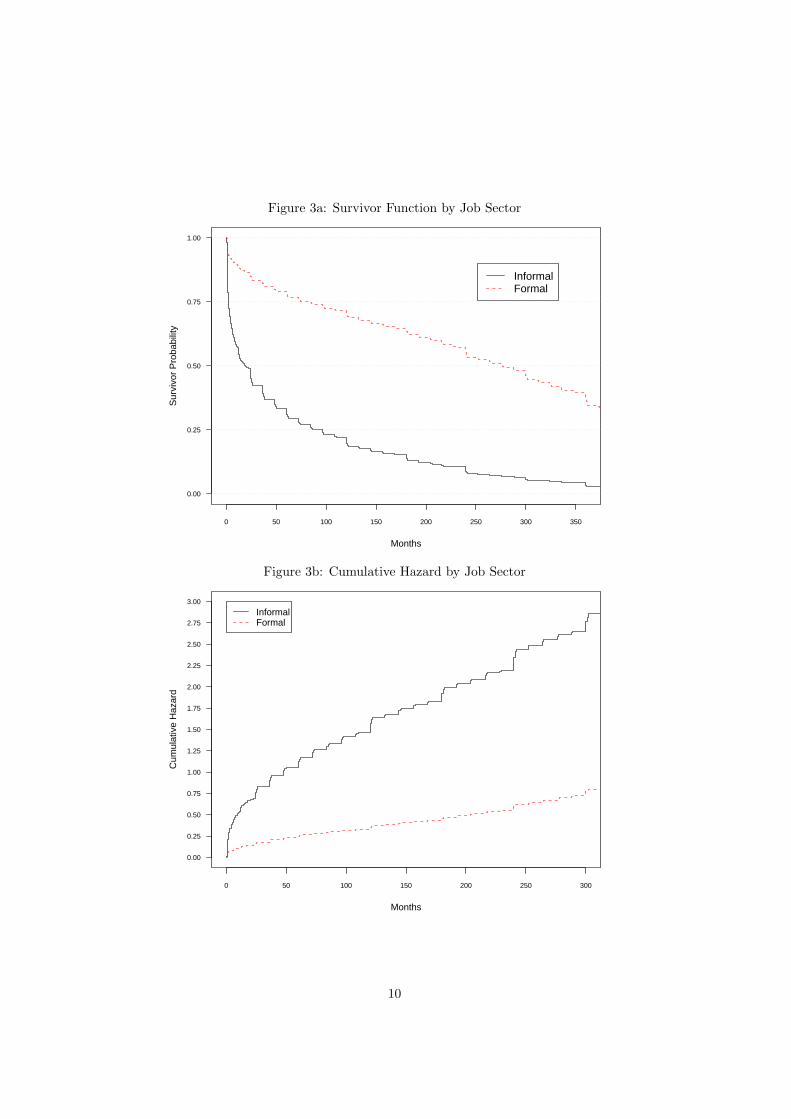
Figure 3a: Survivor Function by Job Sector

0 50 100 150 200 250 300 350

0.00

0.25

0.50

0.75

1.00

Months

Sur

vivo

r P

roba

bilit

y

InformalFormal

Figure 3b: Cumulative Hazard by Job Sector

0 50 100 150 200 250 300

0.00

0.25

0.50

0.75

1.00

1.25

1.50

1.75

2.00

2.25

2.50

2.75

3.00

Months

Cum

ulat

ive

Haz

ard

InformalFormal

10

3 Parametric Analysis of Job Duration

3.1 Methods

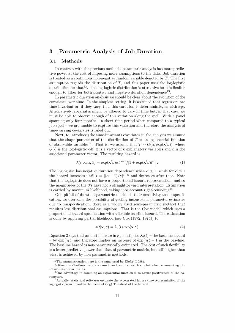
In contrast with the previous methods, parametric analysis has more predic-tive power at the cost of imposing more assumptions to the data. Job durationis treated as a continuous non-negative random variable denoted by T . The firstassumption regards the distribution of T , and this paper uses the log-logisticdistribution for that12. The log-logistic distribution is attractive for it is flexibleenough to allow for both positive and negative duration dependence13.

In parametric duration analysis we should be clear about the evolution of thecovariates over time. In the simplest setting, it is assumed that regressors aretime-invariant or, if they vary, that this variation is deterministic, as with age.Alternatively, covariates might be allowed to vary in time but, in that case, wemust be able to observe enough of this variation along the spell. With a panelspanning only four months – a short time period when compared to a typicaljob spell – we are unable to capture this variation and therefore the analysis oftime-varying covariates is ruled out.

Next, to introduce (the time-invariant) covariates in the analysis we assumethat the shape parameter of the distribution of T is an exponential functionof observable variables14. That is, we assume that T ∼ G(α, exp(x′β)), whereG(·) is the log-logistic cdf, x is a vector of k explanatory variables and β is theassociated parameter vector. The resulting hazard is

λ(t,x;α, β) = exp(x′β)αtα−1/[1 + exp(x′β)tα] . (1)

The loglogistic has negative duration dependence when α ≤ 1, while for α > 1the hazard increases until t = [(α − 1)/γ]1−α and decreases after that. Notethat the loglogistic does not have a proportional hazard representation, and sothe magnitudes of the β’s have not a straightforward interpretation. Estimationis carried by maximum likelihood, taking into account right-censoring15.

One pitfall of duration parametric models is their sensitivity to misspecifi-cation. To overcome the possibility of getting inconsistent parameter estimatesdue to misspecification, there is a widely used semi-parametric method thatrequires less distributional assumptions. That is the Cox model, which uses aproportional hazard specification with a flexible baseline hazard. The estimationis done by applying partial likelihood (see Cox (1972, 1975)) to

λ(t|x, γ) = λ0(t) exp(x′γ). (2)

Equation 2 says that an unit increase in xk multiplies λ0(t) – the baseline hazard– by exp(γk), and therefore implies an increase of exp(γk) − 1 in the baseline.The baseline hazard is non-parametrically estimated. The cost of such flexibilityis a lesser predictive power than that of parametric models, but still higher thanwhat is achieved by non parametric methods.

12The parametrization here is the same used by Kiefer (1988).13Other distributions were also used, and we discuss this point when commenting the

robustness of our results.14One advantage in assuming an exponential function is to assure positiveness of the pa-

rameters.15Actually, statistical softwares estimate the accelerated failure time representation of the

loglogistic, which models the mean of (log) T instead of the hazard.

11

Up to here we have ignored the fact that there are various possible desti-nations to an individual who leaves her job. This is an implicit assumptionof a single risk hazard rate. As Table 2 shows, this might be unrealistic, asthe probabilities of exit vary considerably across destinations. To relax this,we consider a competing independent risks model16. This enables us to lookwith more detail to each possible transition described in Table 2. Of particularinterest to this paper are the formal-informal and informal-formal transitions.

3.2 Results

We first present and discuss results for single risk models. Table 3 shows re-sults for both the full parametric log-logistic model and the semi-parametric Coxmodel. For the Cox model, we report the hazard ratios, i.e., exp(γk) (see equa-tion 2), so exp(γk) > 1 implies positive impacts on the hazard (and thereforea negative impact on expected duration). For the log-logistic model, estimates’signs are as usual: a positive βk implies positive impact on the hazard. There-fore, whenever a coefficient from the log-logistic model is greater than zero, weshould expect exp(γk) > 1 in the Cox model.

Overall, at least two patterns can be identified in Table 3. First, the deter-minants of formal jobs’ duration are somewhat different from those of informaljobs’. For personal characteristics, only the dummies for sex and race havesimilar signs and significance. Schooling and age are either not significant forinformal workers, or have opposite signs. If more qualified and experiencedworkers are those who have more bargain power (or more employment options),then these results indicate that formal jobs are preferred to informal ones. Thesecome from the fact that we observe opposite signs for schooling coefficients inboth sectors, indicating that more qualified workers experience shorter informalspells, while the contrary is true for non-qualified. As for firm characteristics,firm size decreases the hazard rate of both formal and informal job, but is muchmore important for formal jobs. This result points to the importance of thequality of the job to workers mobility: assuming that higher firms offer betterjobs, the higher the job quality the lower the hazard rates out of employment.The differences in dummy sectors are not statistically significant.

Second, the Cox and log-logistic models estimates are in conformity witheach other. Although there are some differences in signs between the two mod-els for informal workers, they are not statistically significant. These resultswere also robust to other distributional assumptions17. As the Cox model isprotected against misspecification, this strengths the case for the log-logistic.The accordance between the models can also be noted in Figures 4a to 4b. Thesurvivor curves predicted by the log-logistic and Cox models are similar in shapeand magnitude for the informal sector, confirming the quality of the parametricfit for this sub-sample. However, the same cannot be said about .

The log-logistic model predicts monotonically decreasing hazards for bothsectors, as α < 1.18 This suggests a tendency to an “informality trap”, as theprobability of exiting an informal job highly decreases over time. If we believethat informal jobs are of inferior quality, then this result is worrisome.

16Assuming correlated risks is a major goal for future research.17Results for the Weibull and exponential models are reported in Table 7 in the Appendix.18As in Section 2, we do not show plots of the predicted hazard because the Cox non-

parametric estimates lack smoothness and are hard to interpret.

12

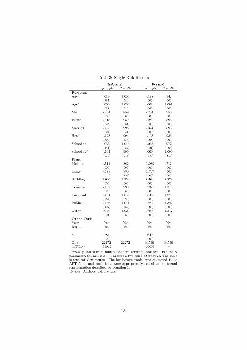
Table 3: Single Risk Results

Informal FormalLog-Logis. Cox PH Log-Logis. Cox PH

PersonalAge .019 1.004 -.188 .942

[.287] [.544] [.000] [.000]

Age2 .000 1.000 .002 1.001[.038] [.019] [.000] [.000]

Man -.404 .859 -.774 .755[.000] [.000] [.000] [.000]

White -.118 .959 -.282 .895[.025] [.031] [.000] [.000]

Married -.035 .998 -.324 .895[.624] [.941] [.000] [.000]

Head -.023 .994 -.193 .933[.709] [.785] [.008] [.009]

Schooling .033 1.014 -.065 .972[.151] [.082] [.021] [.005]

Schooling2 -.004 .999 .000 1.000[.016] [.013] [.986] [.810]

FirmMedium -.511 .862 -1.039 .712

[.000] [.000] [.000] [.000]

Large -.129 .980 -1.707 .562[.014] [.298] [.000] [.000]

Building 1.006 1.350 2.463 2.278[.000] [.000] [.000] [.000]

Comerce -.037 .995 .737 1.313[.626] [.860] [.000] [.000]

Financial -.004 1.052 .646 1.279[.964] [.096] [.000] [.000]

Public -.086 1.011 .723 1.322[.407] [.782] [.000] [.000]

Other .038 1.029 .780 1.347[.601] [.285] [.000] [.000]

Other Ctrls.Year Yes Yes Yes YesRegion Yes Yes Yes Yes

α .781 .649[.000] [.000]

Obs. 22272 22272 54590 54590ln(PLik) -33012 – -40058 –

Notes: p-values from robust standard errors in brackets. For the αparameter, the null is α = 1 against a two-sided alternative. The sameis true for Cox results. The log-logistic model was estimated in itsAFT form, and coefficients were appropriately scaled to the hazardrepresentation described by equation 1.Source: Authors’ calculations.

13

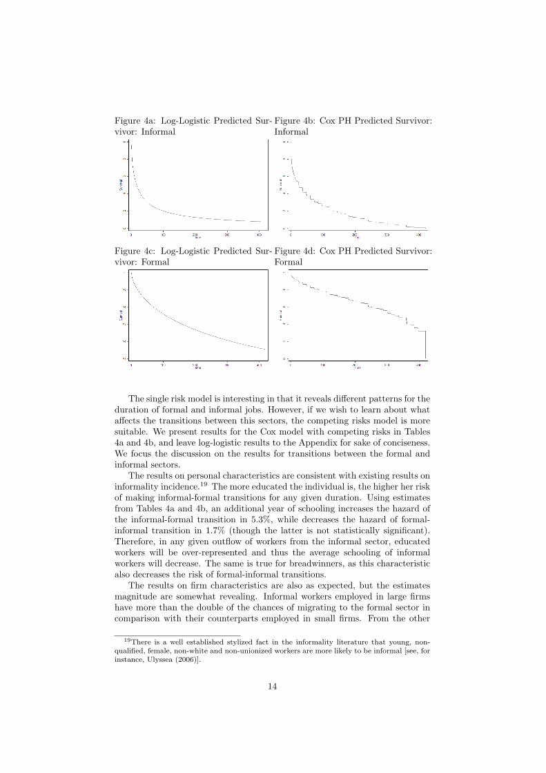
Figure 4a: Log-Logistic Predicted Sur-vivor: Informal

Figure 4b: Cox PH Predicted Survivor:Informal

Figure 4c: Log-Logistic Predicted Sur-vivor: Formal

Figure 4d: Cox PH Predicted Survivor:Formal

The single risk model is interesting in that it reveals different patterns for theduration of formal and informal jobs. However, if we wish to learn about whataffects the transitions between this sectors, the competing risks model is moresuitable. We present results for the Cox model with competing risks in Tables4a and 4b, and leave log-logistic results to the Appendix for sake of conciseness.We focus the discussion on the results for transitions between the formal andinformal sectors.

The results on personal characteristics are consistent with existing results oninformality incidence.19 The more educated the individual is, the higher her riskof making informal-formal transitions for any given duration. Using estimatesfrom Tables 4a and 4b, an additional year of schooling increases the hazard ofthe informal-formal transition in 5.3%, while decreases the hazard of formal-informal transition in 1.7% (though the latter is not statistically significant).Therefore, in any given outflow of workers from the informal sector, educatedworkers will be over-represented and thus the average schooling of informalworkers will decrease. The same is true for breadwinners, as this characteristicalso decreases the risk of formal-informal transitions.

The results on firm characteristics are also as expected, but the estimatesmagnitude are somewhat revealing. Informal workers employed in large firmshave more than the double of the chances of migrating to the formal sector incomparison with their counterparts employed in small firms. From the other

19There is a well established stylized fact in the informality literature that young, non-qualified, female, non-white and non-unionized workers are more likely to be informal [see, forinstance, Ulyssea (2006)].

14

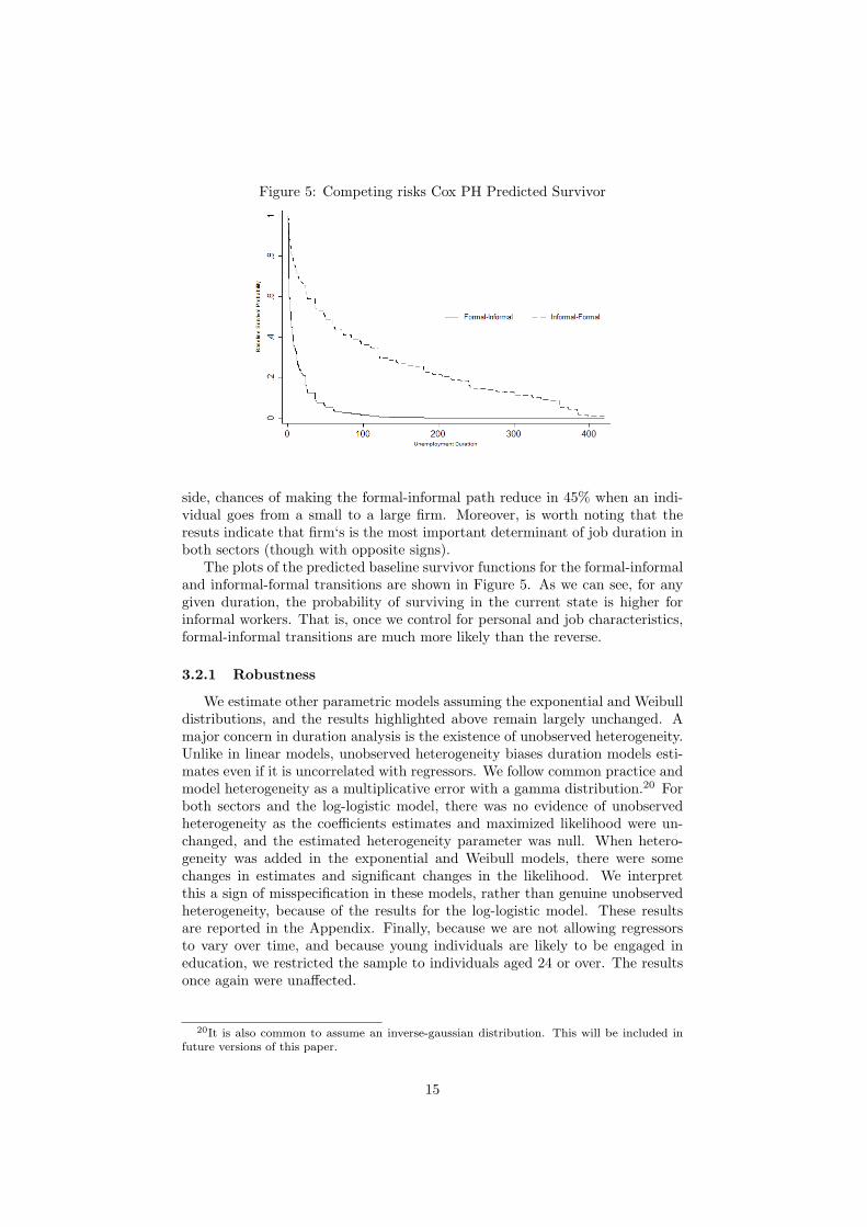
Figure 5: Competing risks Cox PH Predicted Survivor

side, chances of making the formal-informal path reduce in 45% when an indi-vidual goes from a small to a large firm. Moreover, is worth noting that theresuts indicate that firm‘s is the most important determinant of job duration inboth sectors (though with opposite signs).

The plots of the predicted baseline survivor functions for the formal-informaland informal-formal transitions are shown in Figure 5. As we can see, for anygiven duration, the probability of surviving in the current state is higher forinformal workers. That is, once we control for personal and job characteristics,formal-informal transitions are much more likely than the reverse.

3.2.1 Robustness

We estimate other parametric models assuming the exponential and Weibulldistributions, and the results highlighted above remain largely unchanged. Amajor concern in duration analysis is the existence of unobserved heterogeneity.Unlike in linear models, unobserved heterogeneity biases duration models esti-mates even if it is uncorrelated with regressors. We follow common practice andmodel heterogeneity as a multiplicative error with a gamma distribution.20 Forboth sectors and the log-logistic model, there was no evidence of unobservedheterogeneity as the coefficients estimates and maximized likelihood were un-changed, and the estimated heterogeneity parameter was null. When hetero-geneity was added in the exponential and Weibull models, there were somechanges in estimates and significant changes in the likelihood. We interpretthis a sign of misspecification in these models, rather than genuine unobservedheterogeneity, because of the results for the log-logistic model. These resultsare reported in the Appendix. Finally, because we are not allowing regressorsto vary over time, and because young individuals are likely to be engaged ineducation, we restricted the sample to individuals aged 24 or over. The resultsonce again were unaffected.

20It is also common to assume an inverse-gaussian distribution. This will be included infuture versions of this paper.

15

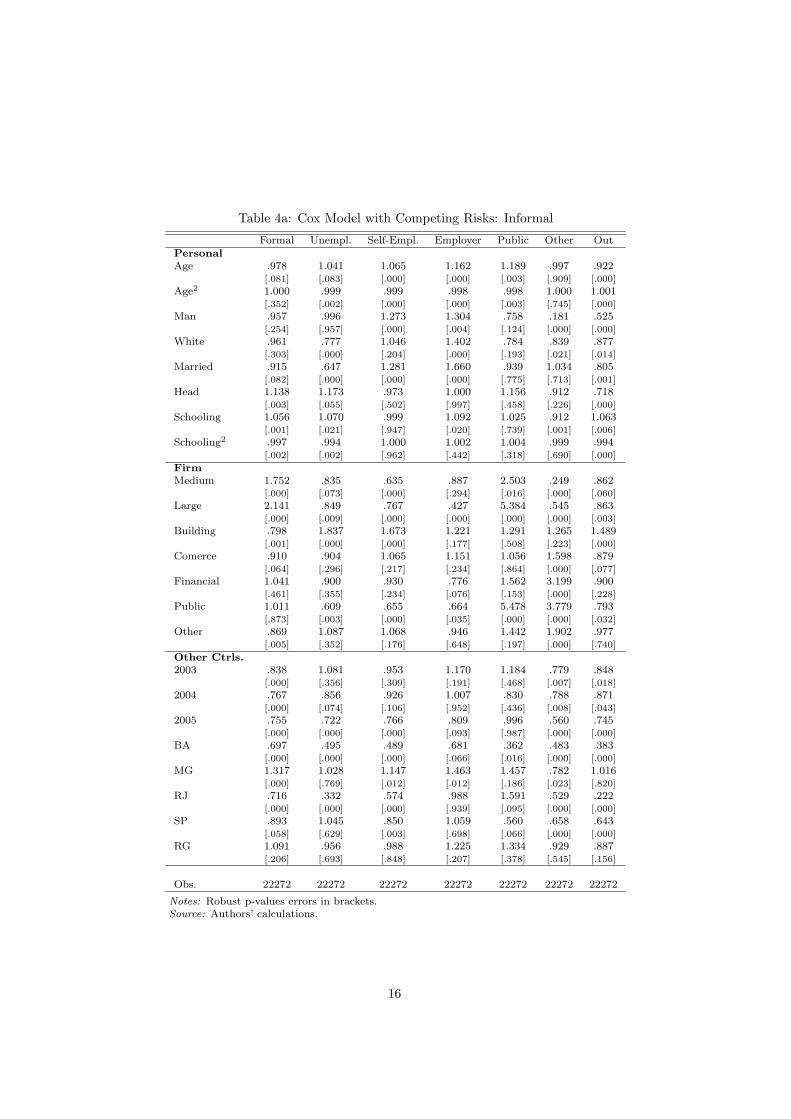
Table 4a: Cox Model with Competing Risks: Informal

Formal Unempl. Self-Empl. Employer Public Other OutPersonalAge .978 1.041 1.065 1.162 1.189 .997 .922

[.081] [.083] [.000] [.000] [.003] [.909] [.000]

Age2 1.000 .999 .999 .998 .998 1.000 1.001[.352] [.002] [.000] [.000] [.003] [.745] [.000]

Man .957 .996 1.273 1.304 .758 .181 .525[.254] [.957] [.000] [.004] [.124] [.000] [.000]

White .961 .777 1.046 1.402 .784 .839 .877[.303] [.000] [.204] [.000] [.193] [.021] [.014]

Married .915 .647 1.281 1.660 .939 1.034 .805[.082] [.000] [.000] [.000] [.775] [.713] [.001]

Head 1.138 1.173 .973 1.000 1.156 .912 .718[.003] [.055] [.502] [.997] [.458] [.226] [.000]

Schooling 1.056 1.070 .999 1.092 1.025 .912 1.063[.001] [.021] [.947] [.020] [.739] [.001] [.006]

Schooling2 .997 .994 1.000 1.002 1.004 .999 .994[.002] [.002] [.962] [.442] [.318] [.690] [.000]

FirmMedium 1.752 .835 .635 .887 2.503 .249 .862

[.000] [.073] [.000] [.294] [.016] [.000] [.060]

Large 2.141 .849 .767 .427 5.384 .545 .863[.000] [.009] [.000] [.000] [.000] [.000] [.003]

Building .798 1.837 1.673 1.221 1.291 1.265 1.489[.001] [.000] [.000] [.177] [.508] [.223] [.000]

Comerce .910 .904 1.065 1.151 1.056 1.598 .879[.064] [.296] [.217] [.234] [.864] [.000] [.077]

Financial 1.041 .900 .930 .776 1.562 3.199 .900[.461] [.355] [.234] [.076] [.153] [.000] [.228]

Public 1.011 .609 .655 .664 5.478 3.779 .793[.873] [.003] [.000] [.035] [.000] [.000] [.032]

Other .869 1.087 1.068 .946 1.442 1.902 .977[.005] [.352] [.176] [.648] [.197] [.000] [.740]

Other Ctrls.2003 .838 1.081 .953 1.170 1.184 .779 .848

[.000] [.356] [.309] [.191] [.468] [.007] [.018]

2004 .767 .856 .926 1.007 .830 .788 .871[.000] [.074] [.106] [.952] [.436] [.008] [.043]

2005 .755 .722 .766 .809 .996 .560 .745[.000] [.000] [.000] [.093] [.987] [.000] [.000]

BA .697 .495 .489 .681 .362 .483 .383[.000] [.000] [.000] [.066] [.016] [.000] [.000]

MG 1.317 1.028 1.147 1.463 1.457 .782 1.016[.000] [.769] [.012] [.012] [.186] [.023] [.820]

RJ .716 .332 .574 .988 1.591 .529 .222[.000] [.000] [.000] [.939] [.095] [.000] [.000]

SP .893 1.045 .850 1.059 .560 .658 .643[.058] [.629] [.003] [.698] [.066] [.000] [.000]

RG 1.091 .956 .988 1.225 1.334 .929 .887[.206] [.693] [.848] [.207] [.378] [.545] [.156]

Obs. 22272 22272 22272 22272 22272 22272 22272

Notes: Robust p-values errors in brackets.Source: Authors’ calculations.

16

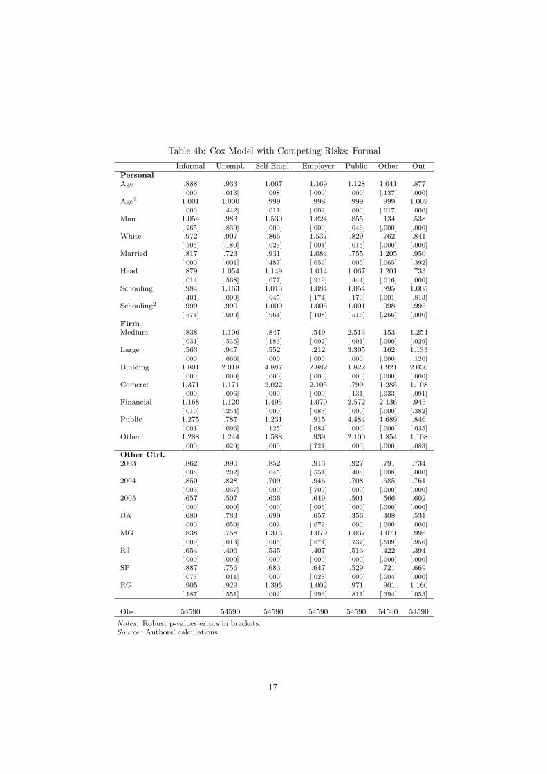
Table 4b: Cox Model with Competing Risks: Formal

Informal Unempl. Self-Empl. Employer Public Other OutPersonalAge .888 .933 1.067 1.169 1.128 1.041 .877

[.000] [.013] [.008] [.000] [.000] [.137] [.000]

Age2 1.001 1.000 .999 .998 .999 .999 1.002[.000] [.442] [.011] [.002] [.000] [.017] [.000]

Man 1.054 .983 1.530 1.824 .855 .134 .538[.265] [.830] [.000] [.000] [.046] [.000] [.000]

White .972 .907 .865 1.537 .829 .762 .841[.505] [.180] [.023] [.001] [.015] [.000] [.000]

Married .817 .723 .931 1.084 .755 1.205 .950[.000] [.001] [.487] [.659] [.005] [.065] [.392]

Head .879 1.054 1.149 1.014 1.067 1.201 .733[.014] [.568] [.077] [.919] [.444] [.016] [.000]

Schooling .984 1.163 1.013 1.084 1.054 .895 1.005[.401] [.000] [.645] [.174] [.170] [.001] [.813]

Schooling2 .999 .990 1.000 1.005 1.001 .998 .995[.574] [.000] [.964] [.108] [.516] [.266] [.000]

FirmMedium .838 1.106 .847 .549 2.513 .153 1.254

[.031] [.535] [.183] [.002] [.001] [.000] [.029]

Large .563 .947 .552 .212 3.305 .162 1.133[.000] [.666] [.000] [.000] [.000] [.000] [.120]

Building 1.801 2.018 4.887 2.882 1.822 1.921 2.036[.000] [.000] [.000] [.000] [.000] [.000] [.000]

Comerce 1.371 1.171 2.022 2.105 .799 1.285 1.108[.000] [.096] [.000] [.000] [.131] [.033] [.091]

Financial 1.168 1.120 1.495 1.070 2.572 2.136 .945[.010] [.254] [.000] [.683] [.000] [.000] [.382]

Public 1.275 .787 1.231 .915 4.484 1.689 .846[.001] [.096] [.125] [.684] [.000] [.000] [.035]

Other 1.288 1.244 1.588 .939 2.100 1.854 1.108[.000] [.020] [.000] [.721] [.000] [.000] [.083]

Other Ctrl.2003 .862 .890 .852 .913 .927 .791 .734

[.008] [.202] [.045] [.551] [.408] [.008] [.000]

2004 .850 .828 .709 .946 .708 .685 .761[.003] [.037] [.000] [.709] [.000] [.000] [.000]

2005 .657 .507 .636 .649 .501 .566 .602[.000] [.000] [.000] [.006] [.000] [.000] [.000]

BA .680 .783 .690 .657 .356 .408 .531[.000] [.050] [.002] [.072] [.000] [.000] [.000]

MG .838 .758 1.313 1.079 1.037 1.071 .996[.009] [.013] [.005] [.674] [.737] [.509] [.956]

RJ .654 .406 .535 .407 .513 .422 .394[.000] [.000] [.000] [.000] [.000] [.000] [.000]

SP .887 .756 .683 .647 .529 .721 .669[.073] [.011] [.000] [.023] [.000] [.004] [.000]

RG .905 .929 1.395 1.002 .971 .901 1.160[.187] [.551] [.002] [.993] [.811] [.394] [.053]

Obs. 54590 54590 54590 54590 54590 54590 54590

Notes: Robust p-values errors in brackets.Source: Authors’ calculations.

17

4 Summary and Future Developments

We estimate reduce-form equations trying to assess the impacts of personaland job characteristics on job duration. The parametric analysis revealed differ-ent patterns for transitions out of the formal and informal sectors. While school-ing and age are positively associated with job duration in the formal sector, theopposite is true for the informal sector. This reinforces the view that informaljobs are of inferior quality, because the more able workers, with a broader menuof job options, are choosing formal jobs. Our findings also point to the existenceof an “informality trap”, as the hazard rates out of informal job decline mono-tonically and quite rapidly over time. This suggest that if the worker does notmove out of informal employment within, say, the first 3-6 months, he is likelyto experience a long informal spell. Moreover, once we disentangle the risks outof informal and informal sectors, we find that informal-formal transitions aresubstantially less likely to happen than the other way around.

More results can be derived from the preceding analysis, and we intend toencompass them in future versions of this paper. Of particular interest is tocompute expected moments (mean and percentiles) of job duration for variouspopulation groups. For that, more flexible specifications, including interactionsbetween covariates, shall be adopted.

References

Ancora, M., D. Coelho, M. Neri, and A. Pinto (1997). Aspectos dinamicos dodesemprego e da posicao na ocupacao. Estudos Economicos 27 (2).

Barros, R., G. Sedlacek, and S. Varanda (1990). Segmentacao e mobilidadeno mercado de trabalho: a carteira de trabalho em sao paulo. Pesquisa ePlanejamento Economico 20 (1).

Carneiro, F. G. and A. Henley (2001). Modelling formal versus informal em-ployment and earnings: microeconomic evidence for brazil. Proceedings ofthe XXIX Brazilian Economy Association Congress.

Christofides, L. N. and C. J. McKenna (1996, April). Unemployment insuranceand job duration in canada. Journal of Labor Economics 14 (2), 286–312.available at http://ideas.repec.org/a/ucp/jlabec/v14y1996i2p286-312.html.

Cox, D. (1972). Regression models and life tables. Journal of the Royal Statis-tical Society B 34, 187–220.

Cox, D. (1975). Regression models and life tables. Biometrika 62 (2), 269–76.

Curi, A. and N. Menezes-Filho (2006). O mercado de trabalho brasileiro e seg-mentado? alteracoes no perfil da informalidade e nos diferenciais de salariosnas decadas de 80 e 90. Estudos Economicos, forthcoming .

Dickens, W. and K. Lang (1988). The reemergence of segmented labor markettheory. The American Economic Review 78 (2), 129–134.

Dickens, W. and K. Lang (1992). Labor market segmentation theory: Recon-sidering the evidence. NBER Working Paper N.4087.

18

Gong, X., A. van Soest, and E. Villagomez (2004). Mobility in the urbanlabor market: A panel data analysis for mexico. Economic Development andCultural Change 53 (1).

Gonzaga, G. (2003). Labor turnover and labor legislation in brazil.Economıa 4 (1).

Kiefer, N. M. (1988). Economic duration data and hazard functions. Journalof Economic Literature 26 (2), 646–79.

Lindeboom, M. and J. Theeuwes (1991, August). Job duration in the nether-lands: The co-existence of high turnover and permanent job attachment.Oxford Bulletin of Economics and Statistics 53 (3), 243–64.

Maloney, W. F. (1999). Does informality imply segmentation in urban labormarkets? evidence from sectoral transitions in mexico. World Bank EconomicReview 13 (2).

Menezes-Filho, N., N. Mendes, and E. Almeida (2004). O diferencial de salariosformal-informal no brasil: Segmentacao ou vies de selecao? Revista Brasileirade Economia 58 (2).

Menezes-Filho, N. and Picchetti (2000). Os determinantes da duracao do de-semprego em Sao Paulo. Pesquisa e Planejamento Economico 30 (1).

Soares, F. (2004). Do informal workers queue for formal jobs in brazil? IPEA,Texto para Discussao N.1021.

Tannuri-Pianto, M. and D. Pianto (2002). Informal employment in brazil: Achoice at the top and segmentation at the botton: a quantile regression ap-proach. Paper presented at the Annual Meeting of the Brazilian EconometricSociety.

Ulyssea, G. (2006). Informalidade no mercado de trabalho brasileiro: umaresenha da literatura. Revista de Economia Polıtica 26 (3).

Van den Berg, G. (2001). Duration models: Specification, identification, andmultiple durations. Handbook of Econometrics 5, 3381–3460.

Appendix

19

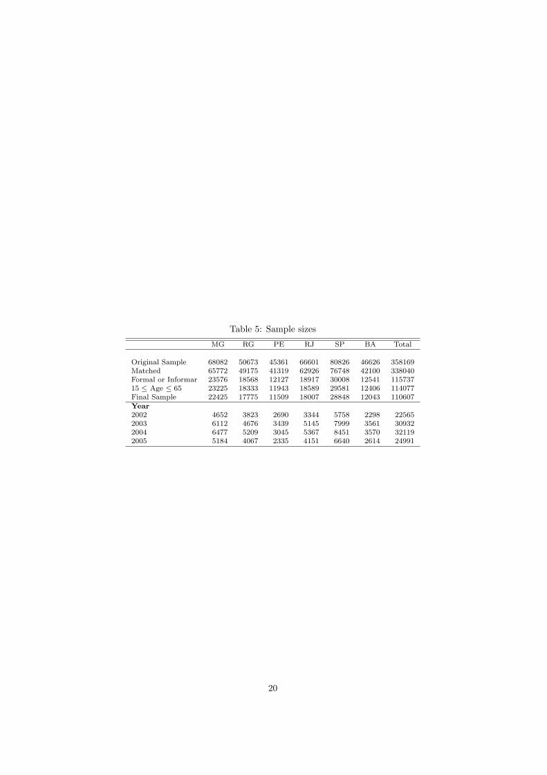
Table 5: Sample sizes

MG RG PE RJ SP BA Total

Original Sample 68082 50673 45361 66601 80826 46626 358169Matched 65772 49175 41319 62926 76748 42100 338040Formal or Informar 23576 18568 12127 18917 30008 12541 11573715 ≤ Age ≤ 65 23225 18333 11943 18589 29581 12406 114077Final Sample 22425 17775 11509 18007 28848 12043 110607Year2002 4652 3823 2690 3344 5758 2298 225652003 6112 4676 3439 5145 7999 3561 309322004 6477 5209 3045 5367 8451 3570 321192005 5184 4067 2335 4151 6640 2614 24991

20

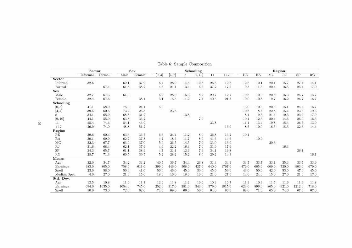
Table 6: Sample Composition

Sector Sex Schooling RegionInformal Formal Male Female [0, 3] [4, 7] 8 [9, 10] 11 +12 PE BA MG RJ SP RG

SectorInformal 32.6 62.1 37.9 6.4 28.9 14.5 10.8 26.6 12.8 12.6 10.1 20.1 15.7 27.4 14.1Formal 67.4 61.8 38.2 4.3 21.1 13.4 6.5 37.2 17.5 9.3 11.3 20.4 16.5 25.4 17.0

SexMale 32.7 67.3 61.9 6.2 28.0 15.3 8.2 29.7 12.7 10.6 10.9 20.6 16.3 25.7 15.7Female 32.4 67.6 38.1 3.1 16.5 11.2 7.4 40.5 21.3 10.0 10.8 19.7 16.2 26.7 16.7

Schooling[0, 3] 41.1 58.9 75.9 24.1 5.0 13.0 10.3 20.5 15.1 24.5 16.7[4, 7] 39.5 60.5 73.2 26.8 23.6 10.6 8.5 22.8 15.4 23.3 19.38 34.1 65.9 68.8 31.2 13.8 8.4 9.3 21.4 19.3 23.9 17.9[9, 10] 44.1 55.9 63.8 36.2 7.9 10.4 12.3 20.4 14.6 26.0 16.311 25.4 74.6 54.1 45.9 33.8 11.1 13.4 19.8 15.4 26.3 13.9+12 26.0 74.0 48.8 51.2 16.0 8.5 10.0 16.5 18.3 32.3 14.4

RegionPE 39.6 60.4 63.3 36.7 6.3 24.4 11.2 8.0 36.8 13.2 10.4BA 30.1 69.9 62.2 37.8 4.7 18.5 11.7 8.9 41.5 14.6 10.9MG 32.3 67.7 63.0 37.0 5.0 26.5 14.5 7.9 33.0 13.0 20.3RJ 31.6 68.4 62.1 37.9 4.6 22.2 16.3 7.0 31.9 17.9 16.3SP 34.3 65.7 61.1 38.9 4.7 21.1 12.6 7.9 34.1 19.8 26.1RG 28.7 71.3 60.5 39.5 5.2 28.2 15.2 8.0 29.2 14.3 16.1

MeansAge 32.0 34.7 34.2 33.2 40.5 36.7 34.4 26.8 31.4 34.4 33.7 33.7 33.1 35.3 33.5 33.9Earnings 483.0 805.0 758.0 611.0 399.0 446.0 508.0 427.0 640.0 1707.0 476.0 605.0 609.0 720.0 903.0 679.0Spell 23.0 58.0 50.0 41.0 50.0 46.0 45.0 30.0 45.0 59.0 43.0 50.0 42.0 53.0 47.0 45.0Median Spell 4.0 27.0 21.0 15.0 18.0 16.0 18.0 10.0 21.0 27.0 14.0 24.0 15.0 27.0 21.0 17.0

Std. Dev.Age 12.5 10.8 11.6 11.1 12.0 11.8 11.2 10.0 10.3 10.7 11.3 10.9 11.5 11.6 11.4 11.8Earnings 694.0 1035.0 1054.0 745.0 252.0 317.0 381.0 343.0 579.0 1915.0 623.0 896.0 865.0 921.0 1212.0 718.0Spell 50.0 73.0 72.0 62.0 74.0 69.0 66.0 50.0 64.0 80.0 68.0 71.0 65.0 74.0 67.0 67.0

21

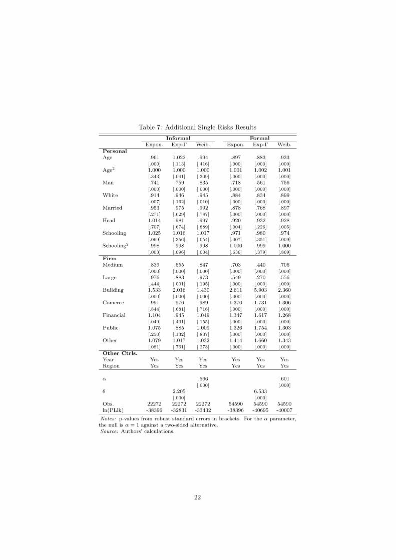
Table 7: Additional Single Risks Results

Informal FormalExpon. Exp-Γ Weib. Expon. Exp-Γ Weib.

PersonalAge .961 1.022 .994 .897 .883 .933

[.000] [.113] [.416] [.000] [.000] [.000]

Age2 1.000 1.000 1.000 1.001 1.002 1.001[.343] [.041] [.309] [.000] [.000] [.000]

Man .741 .759 .835 .718 .561 .756[.000] [.000] [.000] [.000] [.000] [.000]

White .914 .946 .945 .884 .834 .899[.007] [.162] [.010] [.000] [.000] [.000]

Married .953 .975 .992 .878 .768 .897[.271] [.629] [.787] [.000] [.000] [.000]

Head 1.014 .981 .997 .920 .932 .928[.707] [.674] [.889] [.004] [.226] [.005]

Schooling 1.025 1.016 1.017 .971 .980 .974[.069] [.356] [.054] [.007] [.351] [.009]

Schooling2 .998 .998 .998 1.000 .999 1.000[.003] [.096] [.004] [.636] [.379] [.869]

FirmMedium .839 .655 .847 .703 .440 .706

[.000] [.000] [.000] [.000] [.000] [.000]

Large .976 .883 .973 .549 .270 .556[.444] [.001] [.195] [.000] [.000] [.000]

Building 1.533 2.016 1.430 2.611 5.903 2.360[.000] [.000] [.000] [.000] [.000] [.000]

Comerce .991 .976 .989 1.370 1.731 1.306[.844] [.681] [.716] [.000] [.000] [.000]

Financial 1.104 .945 1.049 1.347 1.617 1.268[.049] [.401] [.155] [.000] [.000] [.000]

Public 1.075 .885 1.009 1.326 1.754 1.303[.250] [.132] [.837] [.000] [.000] [.000]

Other 1.079 1.017 1.032 1.414 1.660 1.343[.081] [.761] [.273] [.000] [.000] [.000]

Other Ctrls.Year Yes Yes Yes Yes Yes YesRegion Yes Yes Yes Yes Yes Yes

α .566 .601[.000] [.000]

θ 2.205 6.533[.000] [.000]

Obs. 22272 22272 22272 54590 54590 54590ln(PLik) -38396 -32831 -33432 -38396 -40695 -40007

Notes: p-values from robust standard errors in brackets. For the α parameter,the null is α = 1 against a two-sided alternative.Source: Authors’ calculations.

22

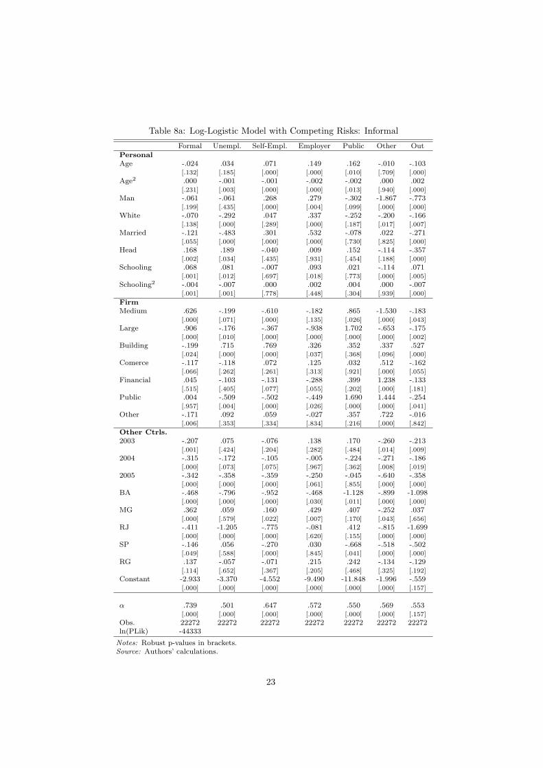
Table 8a: Log-Logistic Model with Competing Risks: Informal

Formal Unempl. Self-Empl. Employer Public Other OutPersonalAge -.024 .034 .071 .149 .162 -.010 -.103

[.132] [.185] [.000] [.000] [.010] [.709] [.000]

Age2 .000 -.001 -.001 -.002 -.002 .000 .002[.231] [.003] [.000] [.000] [.013] [.940] [.000]

Man -.061 -.061 .268 .279 -.302 -1.867 -.773[.199] [.435] [.000] [.004] [.099] [.000] [.000]

White -.070 -.292 .047 .337 -.252 -.200 -.166[.138] [.000] [.289] [.000] [.187] [.017] [.007]

Married -.121 -.483 .301 .532 -.078 .022 -.271[.055] [.000] [.000] [.000] [.730] [.825] [.000]

Head .168 .189 -.040 .009 .152 -.114 -.357[.002] [.034] [.435] [.931] [.454] [.188] [.000]

Schooling .068 .081 -.007 .093 .021 -.114 .071[.001] [.012] [.697] [.018] [.773] [.000] [.005]

Schooling2 -.004 -.007 .000 .002 .004 .000 -.007[.001] [.001] [.778] [.448] [.304] [.939] [.000]

FirmMedium .626 -.199 -.610 -.182 .865 -1.530 -.183

[.000] [.071] [.000] [.135] [.026] [.000] [.043]

Large .906 -.176 -.367 -.938 1.702 -.653 -.175[.000] [.010] [.000] [.000] [.000] [.000] [.002]

Building -.199 .715 .769 .326 .352 .337 .527[.024] [.000] [.000] [.037] [.368] [.096] [.000]

Comerce -.117 -.118 .072 .125 .032 .512 -.162[.066] [.262] [.261] [.313] [.921] [.000] [.055]

Financial .045 -.103 -.131 -.288 .399 1.238 -.133[.515] [.405] [.077] [.055] [.202] [.000] [.181]

Public .004 -.509 -.502 -.449 1.690 1.444 -.254[.957] [.004] [.000] [.026] [.000] [.000] [.041]

Other -.171 .092 .059 -.027 .357 .722 -.016[.006] [.353] [.334] [.834] [.216] [.000] [.842]

Other Ctrls.2003 -.207 .075 -.076 .138 .170 -.260 -.213

[.001] [.424] [.204] [.282] [.484] [.014] [.009]

2004 -.315 -.172 -.105 -.005 -.224 -.271 -.186[.000] [.073] [.075] [.967] [.362] [.008] [.019]

2005 -.342 -.358 -.359 -.250 -.045 -.640 -.358[.000] [.000] [.000] [.061] [.855] [.000] [.000]

BA -.468 -.796 -.952 -.468 -1.128 -.899 -1.098[.000] [.000] [.000] [.030] [.011] [.000] [.000]

MG .362 .059 .160 .429 .407 -.252 .037[.000] [.579] [.022] [.007] [.170] [.043] [.656]

RJ -.411 -1.205 -.775 -.081 .412 -.815 -1.699[.000] [.000] [.000] [.620] [.155] [.000] [.000]

SP -.146 .056 -.270 .030 -.668 -.518 -.502[.049] [.588] [.000] [.845] [.041] [.000] [.000]

RG .137 -.057 -.071 .215 .242 -.134 -.129[.114] [.652] [.367] [.205] [.468] [.325] [.192]

Constant -2.933 -3.370 -4.552 -9.490 -11.848 -1.996 -.559[.000] [.000] [.000] [.000] [.000] [.000] [.157]

α .739 .501 .647 .572 .550 .569 .553[.000] [.000] [.000] [.000] [.000] [.000] [.157]

Obs. 22272 22272 22272 22272 22272 22272 22272ln(PLik) -44333

Notes: Robust p-values in brackets.Source: Authors’ calculations.

23

Table 8b: Log-Logistic Model with Competing Risks: Formal

Informal Unempl. Self-Empl. Employer Public Other OutPersonalAge -.138 -.085 .053 .155 .113 .035 -.147

[.000] [.002] [.031] [.000] [.000] [.229] [.000]

Age2 .001 .001 -.001 -.002 -.001 -.001 .002[.000] [.223] [.060] [.003] [.002] [.053] [.000]

Man .047 -.029 .428 .618 -.134 -2.112 -.652[.335] [.717] [.000] [.000] [.095] [.000] [.000]

White -.028 -.100 -.147 .447 -.161 -.275 -.181[.530] [.174] [.025] [.001] [.040] [.000] [.000]

Married -.217 -.334 -.069 .091 -.289 .175 -.053[.000] [.001] [.513] [.622] [.005] [.107] [.402]

Head -.139 .048 .138 .012 .060 .204 -.335[.011] [.613] [.086] [.934] [.494] [.013] [.000]

Schooling -.015 .154 .019 .089 .069 -.127 .005[.468] [.000] [.509] [.143] [.078] [.000] [.816]

Schooling2 -.001 -.011 .000 .005 .001 -.002 -.006[.498] [.000] [.953] [.116] [.564] [.463] [.000]

FirmMedium -.192 .094 -.186 -.638 .950 -2.056 .218

[.028] [.569] [.152] [.001] [.001] [.000] [.047]

Large -.610 -.066 -.636 -1.619 1.214 -1.990 .111[.000] [.613] [.000] [.000] [.000] [.000] [.192]

Building .655 .762 1.701 1.145 .661 .708 .796[.000] [.000] [.000] [.000] [.000] [.000] [.000]

Comerce .325 .169 .722 .738 -.257 .249 .106[.000] [.080] [.000] [.000] [.083] [.044] [.096]

Financial .158 .130 .409 .048 .937 .776 -.064[.011] [.198] [.000] [.773] [.000] [.000] [.342]

Public .242 -.242 .199 -.112 1.511 .542 -.180[.002] [.097] [.147] [.608] [.000] [.000] [.032]

Other .261 .233 .473 -.062 .733 .666 .109[.000] [.015] [.000] [.730] [.000] [.000] [.076]

Other Ctrl.2003 -.153 -.119 -.162 -.087 -.084 -.254 -.327

[.010] [.201] [.050] [.576] [.372] [.008] [.000]

2004 -.172 -.193 -.359 -.082 -.375 -.407 -.295[.003] [.037] [.000] [.588] [.000] [.000] [.000]

2005 -.442 -.693 -.479 -.458 -.741 -.609 -.542[.000] [.000] [.000] [.005] [.000] [.000] [.000]

BA -.407 -.241 -.399 -.419 -1.037 -.943 -.667[.000] [.059] [.001] [.077] [.000] [.000] [.000]

MG -.190 -.280 .276 .113 .037 .069 -.009[.008] [.014] [.006] [.535] [.737] [.541] [.899]

RJ -.449 -.913 -.669 -.904 -.680 -.942 -.982[.000] [.000] [.000] [.000] [.000] [.000] [.000]

SP -.140 -.286 -.413 -.446 -.691 -.380 -.439[.048] [.011] [.000] [.022] [.000] [.002] [.000]

RG -.105 -.064 .332 .004 -.043 -.114 .149[.184] [.609] [.003] [.985] [.739] [.392] [.066]

Constant -1.256 -3.262 -6.848 -11.188 -10.976 -2.642 -1.174[.000] [.000] [.000] [.000] [.000] [.000] [.000]

α .688 .572 .515 .522 .681 .569 .633[.000] [.000] [.000] [.000] [.000] [.000] [.000]

Obs. 54590 54590 54590 54590 54590 54590 54590ln(PLik) -56387

Notes: Robust p-values errors in brackets.Source: Authors’ calculations.

24

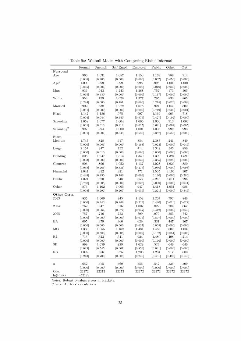
Table 9a: Weibull Model with Competing Risks: Informal

Formal Unempl. Self-Empl. Employer Public Other OutPersonalAge .966 1.031 1.057 1.153 1.169 .989 .914

[0.008] [0.203] [0.000] [0.000] [0.007] [0.650] [0.000]

Age2 1.000 .999 .999 .998 .998 1.000 1.001[0.865] [0.004] [0.000] [0.000] [0.010] [0.930] [0.000]

Man .936 .943 1.243 1.288 .752 .173 .505[0.095] [0.430] [0.000] [0.006] [0.117] [0.000] [0.000]

White .953 .759 1.028 1.377 .795 .833 .865[0.224] [0.000] [0.451] [0.000] [0.215] [0.020] [0.009]

Married .902 .638 1.279 1.678 .924 1.049 .802[0.051] [0.000] [0.000] [0.000] [0.719] [0.609] [0.001]

Head 1.142 1.186 .975 .997 1.169 .903 .718[0.004] [0.044] [0.540] [0.975] [0.427] [0.192] [0.000]

Schooling 1.058 1.077 1.004 1.096 1.030 .913 1.066[0.001] [0.013] [0.812] [0.015] [0.681] [0.002] [0.005]

Schooling2 .997 .994 1.000 1.001 1.003 .999 .993[0.001] [0.001] [0.643] [0.530] [0.387] [0.556] [0.000]

FirmMedium 1.747 .828 .617 .854 2.387 .241 .849

[0.000] [0.066] [0.000] [0.168] [0.023] [0.000] [0.045]

Large 2.151 .847 .752 .414 5.348 .545 .856[0.000] [0.010] [0.000] [0.000] [0.000] [0.000] [0.003]

Building .808 1.947 1.814 1.340 1.399 1.394 1.593[0.003] [0.000] [0.000] [0.049] [0.385] [0.090] [0.000]

Comerce .906 .896 1.052 1.137 1.028 1.629 .880[0.058] [0.266] [0.331] [0.276] [0.930] [0.000] [0.093]

Financial 1.044 .912 .921 .771 1.505 3.196 .907[0.448] [0.430] [0.186] [0.069] [0.190] [0.000] [0.280]

Public 1.021 .620 .648 .653 5.246 3.811 .796[0.768] [0.005] [0.000] [0.028] [0.000] [0.000] [0.041]

Other .873 1.102 1.065 .947 1.418 1.951 .986[0.008] [0.292] [0.207] [0.656] [0.221] [0.000] [0.845]

Other Ctrls.2003 .835 1.069 .945 1.158 1.207 .792 .846

[0.000] [0.443] [0.249] [0.224] [0.420] [0.016] [0.022]

2004 .762 .847 .916 1.007 .822 .784 .867[0.000] [0.064] [0.072] [0.957] [0.412] [0.009] [0.043]

2005 .757 .716 .753 .799 .970 .553 .742[0.000] [0.000] [0.000] [0.077] [0.897] [0.000] [0.000]

BA .695 .479 .460 .629 .331 .447 .367[0.000] [0.000] [0.000] [0.027] [0.009] [0.000] [0.000]

MG 1.330 1.055 1.162 1.481 1.468 .802 1.039[0.000] [0.583] [0.008] [0.009] [0.182] [0.051] [0.608]

RJ .713 .323 .541 .924 1.480 .498 .214[0.000] [0.000] [0.000] [0.609] [0.160] [0.000] [0.000]

SP .899 1.059 .829 1.028 .524 .646 .640[0.083] [0.545] [0.001] [0.853] [0.041] [0.000] [0.000]

RG 1.092 .956 .975 1.206 1.294 .917 .880[0.213] [0.700] [0.689] [0.245] [0.431] [0.488] [0.145]

α .652 .475 .569 .556 .542 .535 .509[0.000] [0.000] [0.000] [0.000] [0.000] [0.000] [0.000]

Obs. 22272 22272 22272 22272 22272 22272 22272ln(PLik) -52129

Notes: Robust p-values errors in brackets.Source: Authors’ calculations.

25

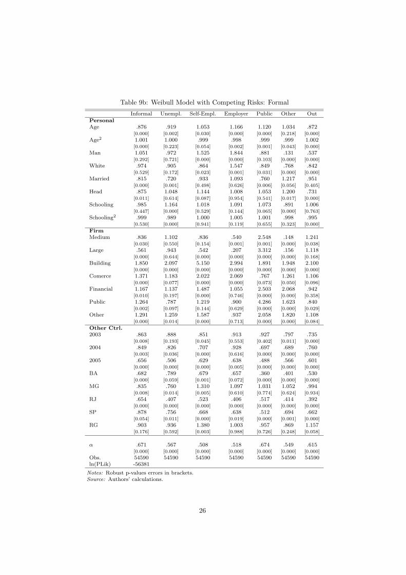
Table 9b: Weibull Model with Competing Risks: Formal

Informal Unempl. Self-Empl. Employer Public Other OutPersonalAge .876 .919 1.053 1.166 1.120 1.034 .872

[0.000] [0.002] [0.030] [0.000] [0.000] [0.218] [0.000]

Age2 1.001 1.000 .999 .998 .999 .999 1.002[0.000] [0.223] [0.054] [0.002] [0.001] [0.043] [0.000]

Man 1.051 .972 1.525 1.844 .881 .131 .537[0.292] [0.721] [0.000] [0.000] [0.103] [0.000] [0.000]

White .974 .905 .864 1.547 .849 .768 .842[0.529] [0.172] [0.023] [0.001] [0.031] [0.000] [0.000]

Married .815 .720 .933 1.093 .760 1.217 .951[0.000] [0.001] [0.498] [0.626] [0.006] [0.056] [0.405]

Head .875 1.048 1.144 1.008 1.053 1.200 .731[0.011] [0.614] [0.087] [0.954] [0.541] [0.017] [0.000]

Schooling .985 1.164 1.018 1.091 1.073 .891 1.006[0.447] [0.000] [0.529] [0.144] [0.065] [0.000] [0.763]

Schooling2 .999 .989 1.000 1.005 1.001 .998 .995[0.530] [0.000] [0.941] [0.119] [0.655] [0.323] [0.000]

FirmMedium .836 1.102 .836 .540 2.548 .148 1.241

[0.030] [0.550] [0.154] [0.001] [0.001] [0.000] [0.038]

Large .561 .943 .542 .207 3.312 .156 1.118[0.000] [0.644] [0.000] [0.000] [0.000] [0.000] [0.168]

Building 1.850 2.097 5.150 2.994 1.891 1.948 2.100[0.000] [0.000] [0.000] [0.000] [0.000] [0.000] [0.000]

Comerce 1.371 1.183 2.022 2.069 .767 1.261 1.106[0.000] [0.077] [0.000] [0.000] [0.073] [0.050] [0.096]

Financial 1.167 1.137 1.487 1.055 2.503 2.068 .942[0.010] [0.197] [0.000] [0.746] [0.000] [0.000] [0.358]

Public 1.264 .787 1.219 .900 4.286 1.623 .840[0.002] [0.097] [0.144] [0.629] [0.000] [0.000] [0.029]

Other 1.291 1.259 1.587 .937 2.058 1.820 1.108[0.000] [0.014] [0.000] [0.713] [0.000] [0.000] [0.084]

Other Ctrl.2003 .863 .888 .851 .913 .927 .797 .735

[0.008] [0.193] [0.045] [0.553] [0.402] [0.011] [0.000]

2004 .849 .826 .707 .928 .697 .689 .760[0.003] [0.036] [0.000] [0.616] [0.000] [0.000] [0.000]

2005 .656 .506 .629 .638 .488 .566 .601[0.000] [0.000] [0.000] [0.005] [0.000] [0.000] [0.000]

BA .682 .789 .679 .657 .360 .401 .530[0.000] [0.059] [0.001] [0.072] [0.000] [0.000] [0.000]

MG .835 .760 1.310 1.097 1.031 1.052 .994[0.008] [0.014] [0.005] [0.610] [0.774] [0.624] [0.934]

RJ .654 .407 .523 .406 .517 .414 .392[0.000] [0.000] [0.000] [0.000] [0.000] [0.000] [0.000]

SP .878 .756 .668 .638 .512 .694 .662[0.054] [0.011] [0.000] [0.019] [0.000] [0.001] [0.000]

RG .903 .936 1.380 1.003 .957 .869 1.157[0.176] [0.592] [0.003] [0.988] [0.726] [0.248] [0.058]

α .671 .567 .508 .518 .674 .549 .615[0.000] [0.000] [0.000] [0.000] [0.000] [0.000] [0.000]

Obs. 54590 54590 54590 54590 54590 54590 54590ln(PLik) -56381

Notes: Robust p-values errors in brackets.Source: Authors’ calculations.

26

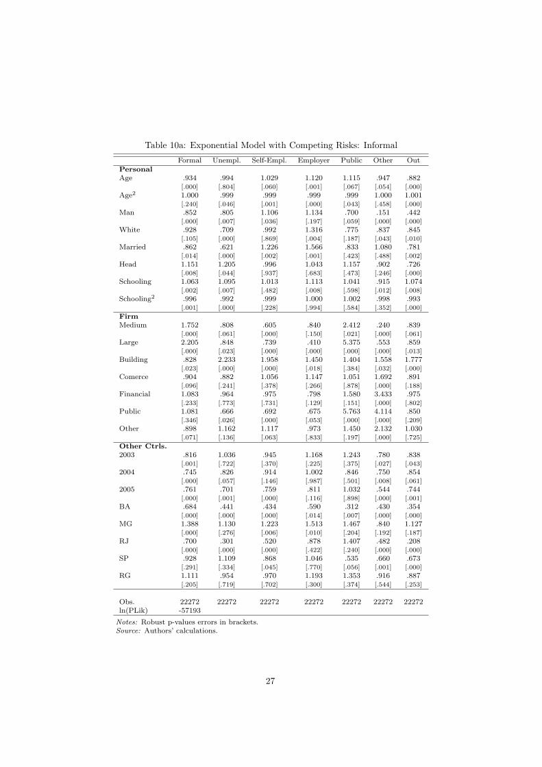
Table 10a: Exponential Model with Competing Risks: Informal

Formal Unempl. Self-Empl. Employer Public Other OutPersonalAge .934 .994 1.029 1.120 1.115 .947 .882

[.000] [.804] [.060] [.001] [.067] [.054] [.000]

Age2 1.000 .999 .999 .999 .999 1.000 1.001[.240] [.046] [.001] [.000] [.043] [.458] [.000]

Man .852 .805 1.106 1.134 .700 .151 .442[.000] [.007] [.036] [.197] [.059] [.000] [.000]

White .928 .709 .992 1.316 .775 .837 .845[.105] [.000] [.869] [.004] [.187] [.043] [.010]

Married .862 .621 1.226 1.566 .833 1.080 .781[.014] [.000] [.002] [.001] [.423] [.488] [.002]

Head 1.151 1.205 .996 1.043 1.157 .902 .726[.008] [.044] [.937] [.683] [.473] [.246] [.000]

Schooling 1.063 1.095 1.013 1.113 1.041 .915 1.074[.002] [.007] [.482] [.008] [.598] [.012] [.008]

Schooling2 .996 .992 .999 1.000 1.002 .998 .993[.001] [.000] [.228] [.994] [.584] [.352] [.000]

FirmMedium 1.752 .808 .605 .840 2.412 .240 .839

[.000] [.061] [.000] [.150] [.021] [.000] [.061]

Large 2.205 .848 .739 .410 5.375 .553 .859[.000] [.023] [.000] [.000] [.000] [.000] [.013]

Building .828 2.233 1.958 1.450 1.404 1.558 1.777[.023] [.000] [.000] [.018] [.384] [.032] [.000]

Comerce .904 .882 1.056 1.147 1.051 1.692 .891[.096] [.241] [.378] [.266] [.878] [.000] [.188]

Financial 1.083 .964 .975 .798 1.580 3.433 .975[.233] [.773] [.731] [.129] [.151] [.000] [.802]

Public 1.081 .666 .692 .675 5.763 4.114 .850[.346] [.026] [.000] [.053] [.000] [.000] [.209]

Other .898 1.162 1.117 .973 1.450 2.132 1.030[.071] [.136] [.063] [.833] [.197] [.000] [.725]

Other Ctrls.2003 .816 1.036 .945 1.168 1.243 .780 .838

[.001] [.722] [.370] [.225] [.375] [.027] [.043]

2004 .745 .826 .914 1.002 .846 .750 .854[.000] [.057] [.146] [.987] [.501] [.008] [.061]

2005 .761 .701 .759 .811 1.032 .544 .744[.000] [.001] [.000] [.116] [.898] [.000] [.001]

BA .684 .441 .434 .590 .312 .430 .354[.000] [.000] [.000] [.014] [.007] [.000] [.000]

MG 1.388 1.130 1.223 1.513 1.467 .840 1.127[.000] [.276] [.006] [.010] [.204] [.192] [.187]

RJ .700 .301 .520 .878 1.407 .482 .208[.000] [.000] [.000] [.422] [.240] [.000] [.000]

SP .928 1.109 .868 1.046 .535 .660 .673[.291] [.334] [.045] [.770] [.056] [.001] [.000]

RG 1.111 .954 .970 1.193 1.353 .916 .887[.205] [.719] [.702] [.300] [.374] [.544] [.253]

Obs. 22272 22272 22272 22272 22272 22272 22272ln(PLik) -57193

Notes: Robust p-values errors in brackets.Source: Authors’ calculations.

27

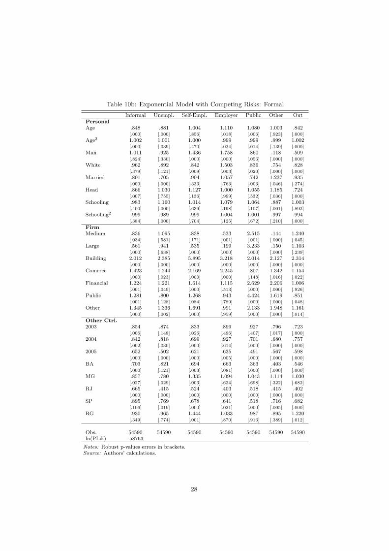
Table 10b: Exponential Model with Competing Risks: Formal

Informal Unempl. Self-Empl. Employer Public Other OutPersonalAge .848 .881 1.004 1.110 1.080 1.003 .842

[.000] [.000] [.856] [.018] [.006] [.923] [.000]

Age2 1.002 1.001 1.000 .999 .999 .999 1.002[.000] [.039] [.470] [.024] [.014] [.139] [.000]

Man 1.011 .925 1.436 1.758 .860 .118 .509[.824] [.330] [.000] [.000] [.056] [.000] [.000]

White .962 .892 .842 1.503 .836 .754 .828[.379] [.121] [.009] [.003] [.020] [.000] [.000]

Married .801 .705 .904 1.057 .742 1.237 .935[.000] [.000] [.333] [.763] [.003] [.046] [.274]

Head .866 1.030 1.127 1.000 1.055 1.185 .724[.007] [.755] [.136] [.999] [.532] [.036] [.000]

Schooling .983 1.160 1.014 1.079 1.064 .887 1.003[.400] [.000] [.639] [.198] [.107] [.001] [.892]

Schooling2 .999 .989 .999 1.004 1.001 .997 .994[.384] [.000] [.704] [.125] [.672] [.210] [.000]

FirmMedium .836 1.095 .838 .533 2.515 .144 1.240

[.034] [.581] [.171] [.001] [.001] [.000] [.045]

Large .561 .941 .535 .199 3.233 .150 1.103[.000] [.638] [.000] [.000] [.000] [.000] [.239]

Building 2.012 2.385 5.895 3.218 2.014 2.127 2.314[.000] [.000] [.000] [.000] [.000] [.000] [.000]

Comerce 1.423 1.244 2.169 2.245 .807 1.342 1.154[.000] [.023] [.000] [.000] [.148] [.016] [.022]

Financial 1.224 1.221 1.614 1.115 2.629 2.206 1.006[.001] [.049] [.000] [.513] [.000] [.000] [.926]

Public 1.281 .800 1.268 .943 4.424 1.619 .851[.001] [.128] [.084] [.789] [.000] [.000] [.048]

Other 1.345 1.336 1.691 .991 2.133 1.948 1.161[.000] [.002] [.000] [.959] [.000] [.000] [.014]

Other Ctrl.2003 .854 .874 .833 .899 .927 .796 .723

[.006] [.148] [.026] [.496] [.407] [.017] [.000]

2004 .842 .818 .699 .927 .701 .680 .757[.002] [.030] [.000] [.614] [.000] [.000] [.000]

2005 .652 .502 .621 .635 .491 .567 .598[.000] [.000] [.000] [.005] [.000] [.000] [.000]

BA .703 .821 .694 .663 .363 .403 .546[.000] [.121] [.003] [.081] [.000] [.000] [.000]

MG .857 .780 1.335 1.094 1.043 1.114 1.030[.027] [.029] [.003] [.624] [.698] [.322] [.682]

RJ .665 .415 .524 .403 .518 .415 .402[.000] [.000] [.000] [.000] [.000] [.000] [.000]

SP .895 .769 .678 .641 .518 .716 .682[.106] [.019] [.000] [.021] [.000] [.005] [.000]

RG .930 .965 1.444 1.033 .987 .895 1.220[.349] [.774] [.001] [.870] [.916] [.389] [.012]

Obs. 54590 54590 54590 54590 54590 54590 54590ln(PLik) -58763

Notes: Robust p-values errors in brackets.Source: Authors’ calculations.

28

Table 11a: Exponential Model with Gamma Heterogeneity and Competing Risks:Informal

Formal Unempl. Self-Empl. Employer Public Other OutPersonalAge 1.019 1.076 1.119 1.195 1.441 .981 .854

[.402] [.125] [.000] [.007] [.001] [.673] [.000]

Age2 .999 .998 .999 .998 .996 1.000 1.002[.001] [.011] [.000] [.021] [.002] [.830] [.000]

Man .926 .867 1.548 1.945 .568 .058 .318[.262] [.267] [.000] [.000] [.082] [.000] [.000]

White .889 .680 1.124 1.947 .793 .876 .861[.081] [.001] [.098] [.000] [.489] [.347] [.135]

Married .834 .460 1.576 2.392 .880 .957 .580[.040] [.000] [.000] [.001] [.760] [.807] [.000]

Head 1.268 1.539 .923 1.127 1.343 .819 .638[.003] [.003] [.323] [.556] [.430] [.173] [.000]

Schooling 1.093 1.131 .956 1.190 .985 .814 1.132[.004] [.024] [.120] [.022] [.903] [.001] [.003]

Schooling2 .995 .990 1.003 1.002 1.012 1.004 .988[.003] [.004] [.097] [.725] [.088] [.270] [.000]

FirmMedium 2.144 .823 .372 .576 4.462 .081 .817

[.000] [.290] [.000] [.022] [.020] [.000] [.189]

Large 3.330 .836 .557 .173 14.545 .391 .770[.000] [.125] [.000] [.000] [.000] [.000] [.007]

Building .903 2.498 2.717 1.968 1.887 1.595 2.359[.405] [.000] [.000] [.028] [.345] [.152] [.000]

Comerce .864 .778 1.186 .945 1.090 1.849 .700[.111] [.148] [.107] [.825] [.880] [.008] [.012]

Financial 1.028 .766 .709 .563 1.640 4.926 .702[.778] [.207] [.008] [.072] [.352] [.000] [.042]

Public .924 .351 .434 .453 16.179 7.183 .663[.513] [.001] [.000] [.053] [.000] [.000] [.037]

Other .772 1.002 1.070 .995 1.936 2.908 .979[.003] [.991] [.514] [.984] [.178] [.000] [.869]

Other Ctrls.2003 .767 1.043 .960 1.191 1.238 .733 .705

[.003] [.784] [.670] [.470] [.634] [.085] [.007]

2004 .688 .778 .887 .928 .664 .715 .755[.000] [.115] [.197] [.757] [.374] [.057] [.026]

2005 .624 .539 .626 .584 .953 .475 .568[.000] [.000] [.000] [.029] [.914] [.000] [.000]

BA .492 .272 .220 .553 .184 .265 .215[.000] [.000] [.000] [.153] [.016] [.000] [.000]

MG 1.666 .945 1.134 2.254 2.317 .660 1.006[.000] [.726] [.225] [.004] [.107] [.041] [.962]

RJ .549 .117 .278 .980 2.908 .214 .064[.000] [.000] [.000] [.946] [.033] [.000] [.000]

SP .762 1.014 .617 1.118 .307 .337 .449[.010] [.929] [.000] [.689] [.032] [.000] [.000]

RG 1.267 .858 .810 1.795 1.013 .591 .872[.054] [.459] [.084] [.062] [.983] [.025] [.393]

θ 4.095 27.032 5.984 3.657 57.874 15.306 14.090[.000] [.000] [.000] [.000] [.000] [.000] [.000]

Obs. 22272 22272 22272 22272 22272 22272 22272ln(PLik) -51790

Notes: Robust p-values errors in brackets.Source: Authors’ calculations.

29

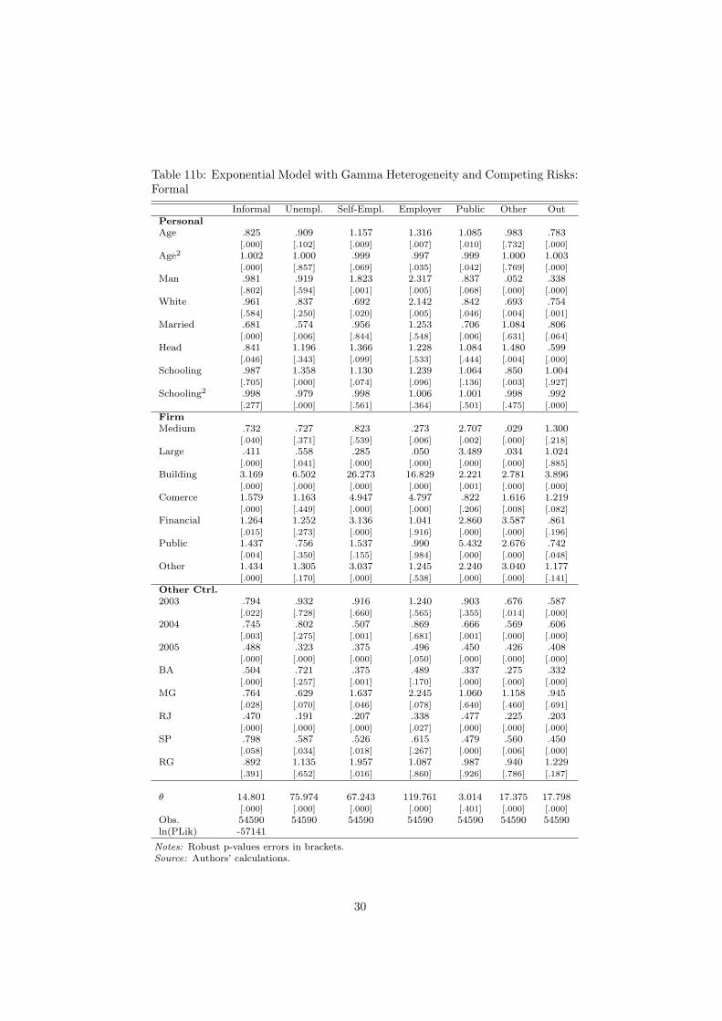
Table 11b: Exponential Model with Gamma Heterogeneity and Competing Risks:Formal

Informal Unempl. Self-Empl. Employer Public Other OutPersonalAge .825 .909 1.157 1.316 1.085 .983 .783

[.000] [.102] [.009] [.007] [.010] [.732] [.000]

Age2 1.002 1.000 .999 .997 .999 1.000 1.003[.000] [.857] [.069] [.035] [.042] [.769] [.000]

Man .981 .919 1.823 2.317 .837 .052 .338[.802] [.594] [.001] [.005] [.068] [.000] [.000]

White .961 .837 .692 2.142 .842 .693 .754[.584] [.250] [.020] [.005] [.046] [.004] [.001]

Married .681 .574 .956 1.253 .706 1.084 .806[.000] [.006] [.844] [.548] [.006] [.631] [.064]

Head .841 1.196 1.366 1.228 1.084 1.480 .599[.046] [.343] [.099] [.533] [.444] [.004] [.000]

Schooling .987 1.358 1.130 1.239 1.064 .850 1.004[.705] [.000] [.074] [.096] [.136] [.003] [.927]

Schooling2 .998 .979 .998 1.006 1.001 .998 .992[.277] [.000] [.561] [.364] [.501] [.475] [.000]

FirmMedium .732 .727 .823 .273 2.707 .029 1.300

[.040] [.371] [.539] [.006] [.002] [.000] [.218]

Large .411 .558 .285 .050 3.489 .034 1.024[.000] [.041] [.000] [.000] [.000] [.000] [.885]

Building 3.169 6.502 26.273 16.829 2.221 2.781 3.896[.000] [.000] [.000] [.000] [.001] [.000] [.000]

Comerce 1.579 1.163 4.947 4.797 .822 1.616 1.219[.000] [.449] [.000] [.000] [.206] [.008] [.082]

Financial 1.264 1.252 3.136 1.041 2.860 3.587 .861[.015] [.273] [.000] [.916] [.000] [.000] [.196]

Public 1.437 .756 1.537 .990 5.432 2.676 .742[.004] [.350] [.155] [.984] [.000] [.000] [.048]

Other 1.434 1.305 3.037 1.245 2.240 3.040 1.177[.000] [.170] [.000] [.538] [.000] [.000] [.141]

Other Ctrl.2003 .794 .932 .916 1.240 .903 .676 .587

[.022] [.728] [.660] [.565] [.355] [.014] [.000]

2004 .745 .802 .507 .869 .666 .569 .606[.003] [.275] [.001] [.681] [.001] [.000] [.000]

2005 .488 .323 .375 .496 .450 .426 .408[.000] [.000] [.000] [.050] [.000] [.000] [.000]

BA .504 .721 .375 .489 .337 .275 .332[.000] [.257] [.001] [.170] [.000] [.000] [.000]

MG .764 .629 1.637 2.245 1.060 1.158 .945[.028] [.070] [.046] [.078] [.640] [.460] [.691]

RJ .470 .191 .207 .338 .477 .225 .203[.000] [.000] [.000] [.027] [.000] [.000] [.000]

SP .798 .587 .526 .615 .479 .560 .450[.058] [.034] [.018] [.267] [.000] [.006] [.000]

RG .892 1.135 1.957 1.087 .987 .940 1.229[.391] [.652] [.016] [.860] [.926] [.786] [.187]

θ 14.801 75.974 67.243 119.761 3.014 17.375 17.798[.000] [.000] [.000] [.000] [.401] [.000] [.000]

Obs. 54590 54590 54590 54590 54590 54590 54590ln(PLik) -57141

Notes: Robust p-values errors in brackets.Source: Authors’ calculations.

30

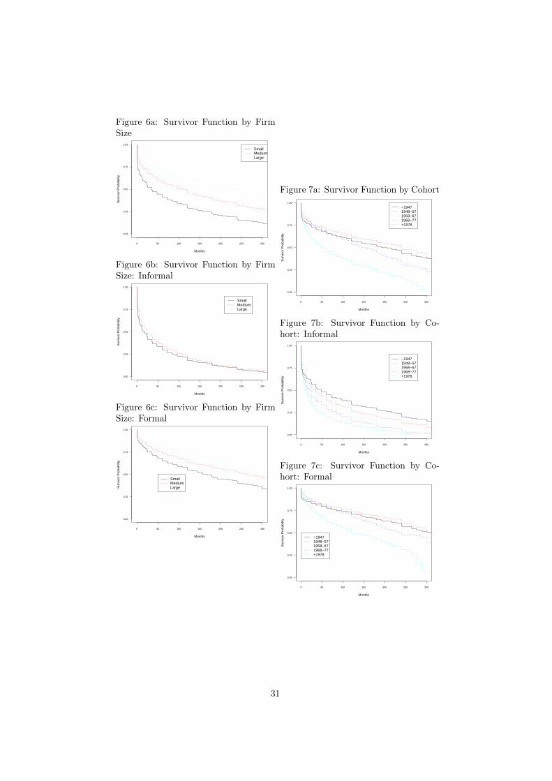
Figure 6a: Survivor Function by FirmSize

0 50 100 150 200 250 300

0.00

0.25

0.50

0.75

1.00

Months

Sur

vivo

r P

roba

bilit

y

SmallMediumLarge

Figure 6b: Survivor Function by FirmSize: Informal

0 50 100 150 200 250 300

0.00

0.25

0.50

0.75

1.00

Months

Sur

vivo

r P

roba

bilit

y

SmallMediumLarge

Figure 6c: Survivor Function by FirmSize: Formal

0 50 100 150 200 250 300

0.00

0.25

0.50

0.75

1.00

Months

Sur

vivo

r P

roba

bilit

y

SmallMediumLarge

Figure 7a: Survivor Function by Cohort

0 50 100 150 200 250 300

0.00

0.25

0.50

0.75

1.00

Months

Sur

vivo

r P

roba

bilit

y

−19471948−571958−671968−77+1978

Figure 7b: Survivor Function by Co-hort: Informal

0 50 100 150 200 250 300

0.00

0.25

0.50

0.75

1.00

Months

Sur

vivo

r P

roba

bilit

y

−19471948−571958−671968−77+1978

Figure 7c: Survivor Function by Co-hort: Formal

0 50 100 150 200 250 300

0.00

0.25

0.50

0.75

1.00

Months

Sur

vivo

r P

roba

bilit

y

−19471948−571958−671968−77+1978

31

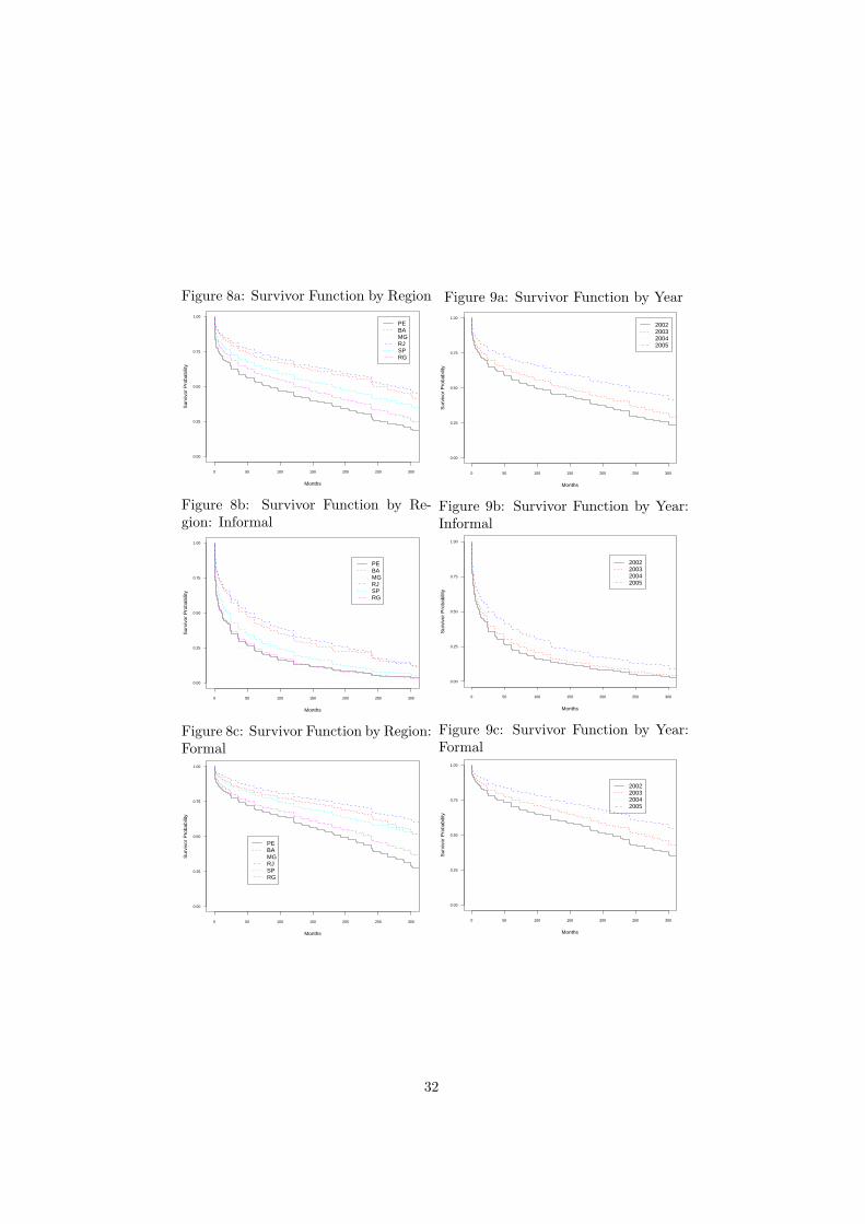
Figure 8a: Survivor Function by Region

0 50 100 150 200 250 300

0.00

0.25

0.50

0.75

1.00

Months

Sur

vivo

r P

roba

bilit

y

PEBAMGRJSPRG

Figure 8b: Survivor Function by Re-gion: Informal

0 50 100 150 200 250 300

0.00

0.25

0.50

0.75

1.00

Months

Sur

vivo

r P

roba

bilit

y

PEBAMGRJSPRG

Figure 8c: Survivor Function by Region:Formal

0 50 100 150 200 250 300

0.00

0.25

0.50

0.75

1.00

Months

Sur

vivo

r P

roba

bilit

y

PEBAMGRJSPRG

Figure 9a: Survivor Function by Year

0 50 100 150 200 250 300

0.00

0.25

0.50

0.75

1.00

Months

Sur

vivo

r P

roba

bilit

y

2002200320042005

Figure 9b: Survivor Function by Year:Informal

0 50 100 150 200 250 300

0.00

0.25

0.50

0.75

1.00

Months

Sur

vivo

r P

roba

bilit

y

2002200320042005

Figure 9c: Survivor Function by Year:Formal

0 50 100 150 200 250 300

0.00

0.25

0.50

0.75

1.00

Months

Sur

vivo

r P

roba

bilit

y

2002200320042005

32