Embed Size (px)
Citation preview
World Wide Webhttps://doi.org/10.1007/s11280-017-0508-3
Joint self-representation and subspace learningfor unsupervised feature selection
Ruili Wang1 · Ming Zong1
Received: 4 September 2017 / Revised: 8 October 2017 / Accepted: 16 October 2017
© Springer Science+Business Media, LLC 2017
Abstract This paper proposes a novel unsupervised feature selection method by joint-ing self-representation and subspace learning. In this method, we adopt the idea ofself-representation and use all the features to represent each feature. A Frobenius norm reg-ularization is used for feature selection since it can overcome the over-fitting problem. TheLocality Preserving Projection (LPP) is used as a regularization term as it can maintain thelocal adjacent relations between data when performing feature space transformation. Fur-ther, a low-rank constraint is also introduced to find the effective low-dimensional structuresof the data, which can reduce the redundancy. Experimental results on real-world datasetsverify that the proposed method can select the most discriminative features and outper-form the state-of-the-art unsupervised feature selection methods in terms of classificationaccuracy, standard deviation, and coefficient of variation.
Keywords Unsupervised feature selection · Self-representation · Subspace learning
1 Introduction
Feature selection is a research hotspot in the fields of pattern analysis, machine learning, anddata mining. The earliest feature selection studies mainly focused on statistical and signalprocessing problems. Since large-scale machine learning emerged in 1990s, existing feature
This article belongs to the Topical Collection: Special Issue on Deep Mining Big Social DataGuest Editors: Xiaofeng Zhu, Gerard Sanroma, Jilian Zhang, and Brent C. Munsell
� Ruili [email protected]
Ming [email protected]
1 Institute of Natural and Mathematical Sciences (INMS), Massey University, Albany, Auckland,New Zealand
(2018) 21:1745–1758
/Published online: 6 November 2017
selection algorithms had diffract to meet the challenge [26]. When the number of featuresreaches a certain size, the accuracy of a classifier is declining, which is called the curseof dimensionality [1, 19, 36]. Therefore, there is an urgent need to develop better featureselection algorithms to increase the accuracy and efficiency for the large-scale data.
Feature selection is a method of selecting some of features that have more discriminativeability from a set of features to reduce the dimension of a feature space. It is an importantcomponent of a classification system [21, 27]. For a classification system, a good learningsample is the key in training a classifier. The quality of the data, for example, whether thesample contains irrelevant or redundant features can directly affect the performance of theclassifier [29, 30]. Therefore, it is important to develop an effective feature selection method.
In general, based on the combination of subset evaluation criteria in feature selectionand follow-up learning algorithms, the feature selection approaches can be categorized intothree groups: the filter approach, wrapper approach and embedded approach. The filterapproach [10] is independent of the follow-up learning algorithm and it uses the statisti-cal performance of all training samples to evaluate the features [17]. The time cost of thefilter approach is low, but the evaluation may have a deviation with the follow-up learn-ing algorithm. While the wrapper approach [10, 18] uses the follow-up learning algorithmto evaluate the accuracy of the training features, the deviation is thus small, but the com-putation cost is large and thus not suitable for a large-scale data set [31]. In the embeddedfeature selection approach [7], a feature selection method itself is embedded as a compo-nent into a learning algorithm. The most typical embedded method is a decision tree [30].However, the key of feature selection methods depend on the efficient selection of a usefulsubset of features. The features in this selected feature subset are kept while remaining fea-tures are abandoned. However, the abandoned features may also be related to other features,while the abandonment may lose some useful relevant information. Further, it is helpful forfeature selection to effectively utilize the relation between data.
In order to utilize the relation between data, firstly, self-representation has been widelyused for feature selection [33], according to self-similarity, i.e., a feature can be repre-sented by all other features. Then, subspace learning is also introduced for keeping therelevance between data [9, 12, 35]. Subspace learning is designed to maintain specific sta-tistical properties such as Principal Component Analysis (PCA) [37], Linear DiscriminantAnalysis (LDA) and so on when performing feature space transformation. These subspacelearning methods can effectively mitigate the so-called curse of dimensionality and preservethe inherent relevance of the data. Thus, the above two points motivate this paper to con-sider taking advantages of the merits of both self-representation and subspace learning as awhole.
Therefore, this paper proposed a new Unsupervised Feature selection method by jointingSelf-representation and Subspace learning, which is called UFSS for short. Firstly, becauseof the correlation between features, we consider using all features to represent each fea-ture, that is, each feature is reconstructed by all features. Correspondingly, we use the leastsquares method as a loss function to evaluate the reconstruction error. Then, in order toovercome the over-fitting problem and select the most discriminative features, we use theFrobenius norm to constrain the reconstruction coefficient matrix to overcome the over-fitting problem and select the most discriminative features. On the other hand, we introduceLocality Preserving Projection (LPP) as a regularization term to maintain the local adjacentrelation of the data when performing feature space transformation during the reconstructionprocess [11]. At the same time, we consider further applying a low-rank constraint to findthe effective low-dimensional structures of the data, which can reduce the redundancy [34].Finally, we proposed an effective optimization method to solve the objective function fast.
World Wide Web (2018) 21:1745–17581746
In summarization, the core of feature selection methods is to select the most effectivefeatures from the original features to reduce the feature dimension, which is a key datapreprocessing step in pattern recognition. Based on the selected optimal feature subset, weuse a classic classifier, i.e., Support Vector Machine (SVM), to classify the test samples.
The rest of this paper is organized as follows: We briefly review the previous featureselection methods and subspace learning methods in Section 2. After that, in Section 3, wegive the details of the proposed new unsupervised feature selection method UFSS. Then, wepresent the experimental results in Section 4. Finally, we summarize our work and futurework in Section 5.
2 Related work
In this section, we briefly review three important items: unsupervised feature selection,subspace learning and self-representation, because our proposed algorithm is based on themand they play different roles during the reconstruction.
2.1 Unsupervised feature selection
Supervised feature selection methods use the class labels as a guide to achieve featureselection. However, a lot of data may be unlabeled in a practical application. Therefore,unsupervised feature selection methods are useful and more difficult because they do nothave class labels to use. Tabakhi et al. [19] proposed an ant colony algorithm, which can pro-vide a well approximate solution based on previous iterations and the time cost is acceptable.Liu et al. [13] drew lessons from the Laplacian Score method. They considered replacing thek-means clustering method with a distance-based entropy measure in the Laplacian Score(LS) for automatically selecting the optimal subset of features. Qian and Zhai [16] tookadvantages of local learning and nonnegative matrix factorization. The proposed methodcan select the most discriminative subset of features by combining robust clustering androbust feature selection at the same time. Based on manifold learning and sparse learningmodel, Cai et al. [3] proposed Multi-Cluster Feature Selection (MCFS)). They consideredusing spectral analysis methods based on the preserved multi-cluster structure of the data tomeasure the relevance between different features.
2.2 Subspace learning
Subspace learning has been applied in different kinds of models for reducing dimension.Zou et al. [39] proposed a new improved principal component analysis based on sparsecoding, which is called sparse principal component analysis (SPCA). It uses Lasso penaltyto produce sparse principal component. Yan et al. [24] considered using graph embeddingtechnology to represent the geometric structure or properties of the sample space. Based onit, they applied it to characterize intraclass compactness and interclass separability simulta-neously and can better solve the problem that the number of available projection directionsis low in LDA. Recently, Nikitidis et al. [15] proposed a method called maximum mar-gin projection pursuit. It can take advantage of maximum margin to discriminate sampleswhen performing feature space transformation. Cai et al. [2] proposed to use both graphembedding and regression for sparse projections learning, it can solve different graph-basedsubspace learning methods by the proposed unified framework.
World Wide Web (2018) 21:1745–1758 1747
2.3 Self-representation
Self-representation stems from the natural self-similarity phenomenon [33], which meansthat a part of an object is similar to other parts of the object, such as coastlines, stock marketmovements and so on. Just like sparsity results in sparse representation, self-similarity leadsto self-representation. Of course, self-representation has been widely used for high dimen-sional data. Zhu et al. [33] proposed to use self-representation and �2,1-norm to constrainthe coefficient matrix for removing outliers and can select the most representative featuresto reconstruct other features. Zhang et al. [28] proposed a new improved kNNmethod basedself-representation, which also uses training samples to reconstruct themselves and imposes�1-norm to make representation coefficient matrix to produce sparsity.
3 Approach
In this section, firstly, we give some notations used in this paper in Section 3.1 and give somebasic knowledge as preliminary in Section 3.2. The details of the proposed UFSS methodis described in Section 3.3. We presented an optimization method to solve the objectivefunction in Section 3.4. Finally, we analyze the convergence of the objective function inSection 3.5.
3.1 Notations
In this paper, we denote scalars as normal italic letters, vectors as bold lowercase lettersand matrices as bold uppercase letters, respectively [29, 30]. Given a matrix X = [xij ], wedenote the ith row of X by xi , and the j th column of X by xj . The Frobenius norm and
�1-norm of X are defined as ||X||F =√∑
i ||xi ||22 =√∑
j ||xj ||22 (matrix norms here are
entry-wise norm), ||X||1 =√∑
i
∑j |xij | and ||X||21 = ∑
i
√∑j x2ij . The trace operator,
the transpose operator and the inverse of X is denoted as tr(X), XT and X−1, respectively.
3.2 Preliminary
Let X ∈ Rn×d denotes a sample matrix, where n and d denote the numbers of samples
and features, respectively. We also use x1, x2,..., xn to denote the n samples where is acolumn vector, thus X = [x1; x2; ...; xn]. On the other hand, we use f1, f2, ..., fd to denotethe d features and f1, f2, ..., fd are the corresponding feature vectors, where fi ∈ R
n andX = [f1, f2, ..., fd ].
The key of unsupervised feature selection methods is to select an optimal feature subsetfor all the samples. Drawn lessons from the regression problem [28, 33], we can regard thefeature selection problem as a regression problem [33]:
minW
l(XW − Y) + λR(W) (1)
where W denotes a coefficient matrix, which is used to measure the weight of a feature.Y usually is a response matrix and l(XW − Y) denotes a loss function. R(W) usually is aregularization imposed on W and λ is a positive constant.
World Wide Web (2018) 21:1745–17581748
3.3 UFSS method
Many developed feature selection methods are derived from the model in (1), althoughconsidering correlation between features, it is still hard to select the proper response matrixY. Drawing lessons from the merits of both self-representation and subspace learning, inthis section, we proposed a new combined method for unsupervised feature selection. Theself-representation denotes that the proposed method uses the sample matrix X instead ofthe response matrix Y, i.e., Y = X, which means each feature can be represented by all thefeatures. Therefore, we can represent each feature fi as follow:
fi =d∑
j=1
fjwji + ei (2)
Applied to all the features, then (2) can also be represented in a matrix form as follow:
X = XW + eb (3)
where W = [wji] ∈ Rd×d is the self-representation coefficients matrix, e ∈ R
n×1 denotes acolumn vector with all elements are 1 and b ∈ R
1×d is a bias term. Obviously, in order to useXW to represent X sufficiently, we should make error term eb as small as possible. Frobe-nius norm can be adopted to measure the residual, i.e., min
W,b||X − XW − eb||F . The matrix
W reflects the importance of different features. To avoid over-fitting and to select the mostdiscriminative features, absorbing the core idea from ridge regression [29, 30], a shrink reg-ularization factor is introduced, i.e., ||W||F . In addition, as the basic assumption of manifoldlearning, a classic method of subspace learning, we know that real data may be presented ina high-dimensional structure but actually it may exist in a very low-dimensional manifold,i.e., the data can be represented by low-dimensional structure to some extent if we can mapit back into the low dimensional space and reveal its essence. Taking advantage of mani-fold learning, locality preserving projection (LPP) as a regularization term is introduced tomaintain the local adjacent relations of the data after performing feature space transforma-tion during the self-representation process [32, 38]. Then we can have the objective functionas follow:
minW,b
||X − XW − eb||F + λ1||W||F + λ2tr(WT XT LXW) (4)
where λ1 and λ2 are control parameters. The penalty term ||W||F is used for penalizing allcoefficients in W together; L = D−S ∈ R
d×d is called graph Laplacian, where S ∈ Rd×d is
a similarity matrix and D ∈ Rd×d is a diagonal matrix. On the other hand, in order to further
remove the large amount of redundancy in the data, a low rank constraint is introduced tofind the effective low-dimensional structures of the data, which can guarantee to reduce theredundancy. Thus, the low rank constraint can be applied to the rank of W, i.e.,
rank(W) = r, r ≤ min(n, d) (5)
Further, (5) can be re-expressed as product of two r − rank matrices as follow:
W = AB (6)
World Wide Web (2018) 21:1745–1758 1749
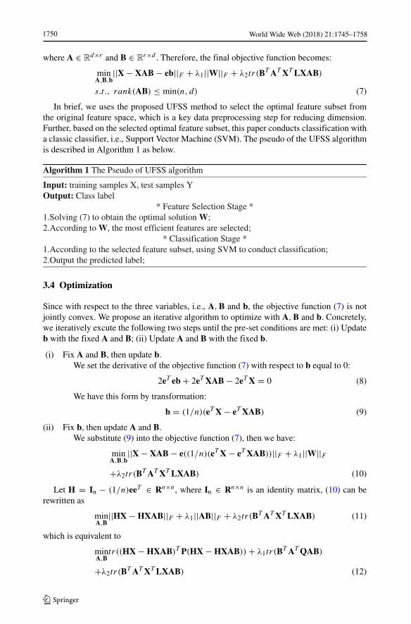
where A ∈ Rd×r and B ∈ R
r×d . Therefore, the final objective function becomes:
minA,B,b
||X − XAB − eb||F + λ1||W||F + λ2tr(BT AT XT LXAB)
s.t., rank(AB) ≤ min(n, d) (7)
In brief, we uses the proposed UFSS method to select the optimal feature subset fromthe original feature space, which is a key data preprocessing step for reducing dimension.Further, based on the selected optimal feature subset, this paper conducts classification witha classic classifier, i.e., Support Vector Machine (SVM). The pseudo of the UFSS algorithmis described in Algorithm 1 as below.
3.4 Optimization
Since with respect to the three variables, i.e., A, B and b, the objective function (7) is notjointly convex. We propose an iterative algorithm to optimize with A, B and b. Concretely,we iteratively excute the following two steps until the pre-set conditions are met: (i) Updateb with the fixed A and B; (ii) Update A and B with the fixed b.
(i) Fix A and B, then update b.We set the derivative of the objective function (7) with respect to b equal to 0:
2eT eb + 2eT XAB − 2eT X = 0 (8)
We have this form by transformation:
b = (1/n)(eT X − eT XAB) (9)
(ii) Fix b, then update A and B.We substitute (9) into the objective function (7), then we have:
minA,B,b
||X − XAB − e((1/n)(eT X − eT XAB))||F + λ1||W||F+λ2tr(BT AT XT LXAB) (10)
Let H = In − (1/n)eeT ∈ Rn×n, where In ∈ Rn×n is an identity matrix, (10) can berewritten as
minA,B
||HX − HXAB||F + λ1||AB||F + λ2tr(BT AT XT LXAB) (11)
which is equivalent to
minA,B
tr((HX − HXAB)T P(HX − HXAB)) + λ1tr(BT AT QAB)
+λ2tr(BT AT XT LXAB) (12)
World Wide Web (2018) 21:1745–17581750
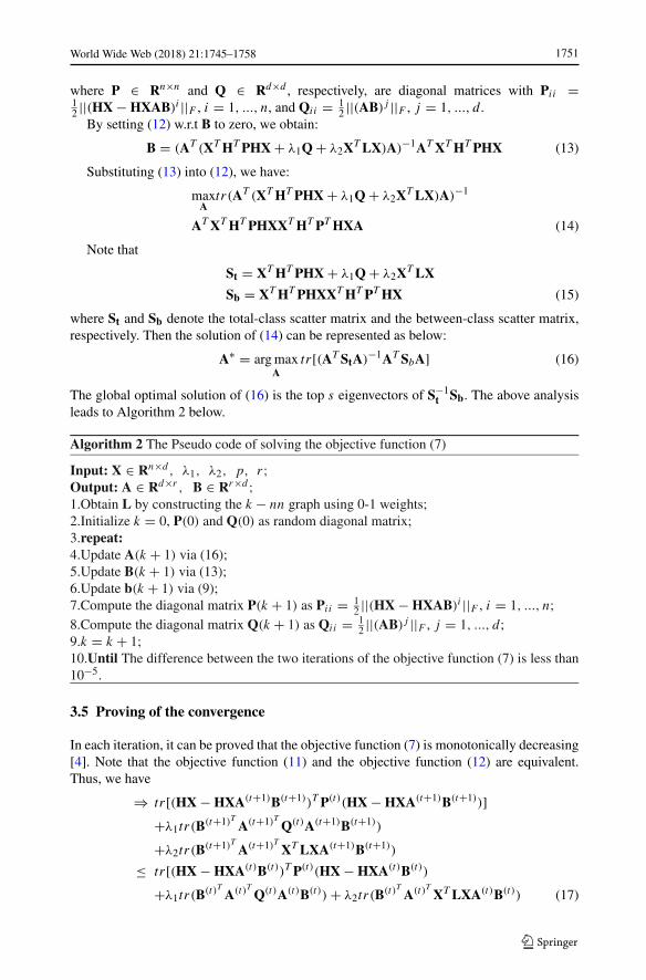
where P ∈ Rn×n and Q ∈ Rd×d , respectively, are diagonal matrices with Pii =12 ||(HX − HXAB)i ||F , i = 1, ..., n, and Qii = 1
2 ||(AB)j ||F , j = 1, ..., d.By setting (12) w.r.t B to zero, we obtain:
B = (AT (XT HT PHX + λ1Q + λ2XT LX)A)−1AT XT HT PHX (13)
Substituting (13) into (12), we have:
maxA
tr(AT (XT HT PHX + λ1Q + λ2XT LX)A)−1
AT XT HT PHXXT HT PT HXA (14)
Note that
St = XT HT PHX + λ1Q + λ2XT LX
Sb = XT HT PHXXT HT PT HX (15)
where St and Sb denote the total-class scatter matrix and the between-class scatter matrix,respectively. Then the solution of (14) can be represented as below:
A∗ = argmaxA
tr[(AT StA)−1AT SbA] (16)
The global optimal solution of (16) is the top s eigenvectors of S−1t Sb. The above analysis
leads to Algorithm 2 below.
3.5 Proving of the convergence
In each iteration, it can be proved that the objective function (7) is monotonically decreasing[4]. Note that the objective function (11) and the objective function (12) are equivalent.Thus, we have
⇒ tr[(HX − HXA(t+1)B(t+1))T P(t)(HX − HXA(t+1)B(t+1))]+λ1tr(B(t+1)T A(t+1)T Q(t)A(t+1)B(t+1))
+λ2tr(B(t+1)T A(t+1)T XT LXA(t+1)B(t+1))
≤ tr[(HX − HXA(t)B(t))T P(t)(HX − HXA(t)B(t))
+λ1tr(B(t)T A(t)T Q(t)A(t)B(t)) + λ2tr(B(t)T A(t)T XT LXA(t)B(t)) (17)
World Wide Web (2018) 21:1745–1758 1751
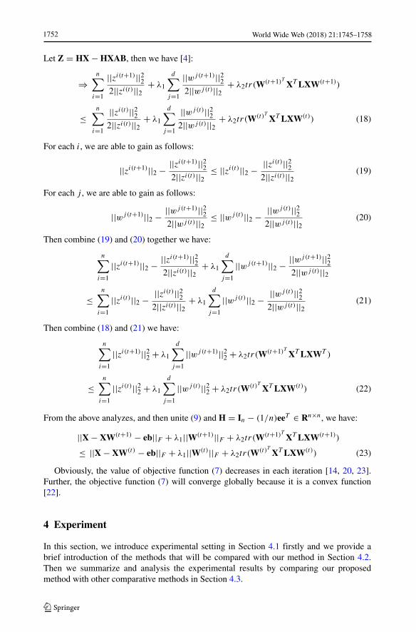
Let Z = HX − HXAB, then we have [4]:
⇒n∑
i=1
||zi(t+1)||222||zi(t)||2 + λ1
d∑j=1
||wj(t+1)||222||wj(t)||2 + λ2tr(W(t+1)T XT LXW(t+1))
≤n∑
i=1
||zi(t)||222||zi(t)||2 + λ1
d∑j=1
||wj(t)||222||wj(t)||2 + λ2tr(W(t)T XT LXW(t)) (18)
For each i, we are able to gain as follows:
||zi(t+1)||2 − ||zi(t+1)||222||zi(t)||2 ≤ ||zi(t)||2 − ||zi(t)||22
2||zi(t)||2 (19)
For each j , we are able to gain as follows:
||wj(t+1)||2 − ||wj(t+1)||222||wj(t)||2 ≤ ||wj(t)||2 − ||wj(t)||22
2||wj(t)||2 (20)
Then combine (19) and (20) together we have:
n∑i=1
||zi(t+1)||2 − ||zi(t+1)||222||zi(t)||2 + λ1
d∑j=1
||wj(t+1)||2 − ||wj(t+1)||222||wj(t)||2
≤n∑
i=1
||zi(t)||2 − ||zi(t)||222||zi(t)||2 + λ1
d∑j=1
||wj(t)||2 − ||wj(t)||222||wj(t)||2 (21)
Then combine (18) and (21) we have:
n∑i=1
||zi(t+1)||22 + λ1
d∑j=1
||wj(t+1)||22 + λ2tr(W(t+1)T XT LXWT )
≤n∑
i=1
||zi(t)||22 + λ1
d∑j=1
||wj(t)||22 + λ2tr(W(t)T XT LXW(t)) (22)
From the above analyzes, and then unite (9) and H = In − (1/n)eeT ∈ Rn×n, we have:
||X − XW(t+1) − eb||F + λ1||W(t+1)||F + λ2tr(W(t+1)T XT LXW(t+1))
≤ ||X − XW(t) − eb||F + λ1||W(t)||F + λ2tr(W(t)T XT LXW(t)) (23)
Obviously, the value of objective function (7) decreases in each iteration [14, 20, 23].Further, the objective function (7) will converge globally because it is a convex function[22].
4 Experiment
In this section, we introduce experimental setting in Section 4.1 firstly and we provide abrief introduction of the methods that will be compared with our method in Section 4.2.Then we summarize and analysis the experimental results by comparing our proposedmethod with other comparative methods in Section 4.3.
World Wide Web (2018) 21:1745–17581752
Table 1 Datasets summarizationDatasets Instance Feature Class
SPECTF Heart 267 44 2
LungCancer 32 56 2
Sonar 208 60 2
Movements 360 90 15
USPS 9298 256 10
Arrhythmia 452 279 13
Yeast 1484 1470 10
FERET 1400 6400 200
4.1 Experimental setting
The experimental environment is a Window XP system, and Matlab 7.11.0 is used to imple-ment all the algorithms. In our experiments, we conduct the 10-fold cross-validation methodfor all methods. The final result was computed by averaging the results from all experiments.We apply the proposed UFSS method and the comparison methods to the classificationtask and evaluate them on eight datasets in terms of three different evaluations, i.e., classi-fication accuracy, STandard Deviation (STD) and coefficient of variation. Specifically, wecompare our methods with other methods in dimension reduction for feature selection, andthen we use Support Vector Machine (SVM) [25] to conduct classification via the LIB-SVM toolbox.1 These datasets contain binary datasets and multi-class datasets, includingSPECTF Heart, LungCancer, Sonar, Movements, Arrhythmia and Yeast. They are all down-loaded from UCI Machine Learning Repository,2 the USPS dataset is downloaded from thewebsite of Feature Selection Data sets,3 while the FERET dataset is downloaded from thewebsite of CSDN.4 We summarized datasets in Table 1.
Three kinds of evaluation metrics as the evaluations for the classification task, i.e., clas-sification accuracy, STandard Deviation (STD for short) and Coefficient of Variation (CVfor short), respectively. The higher accuracy the algorithm is, the better classification per-formance it is. The smaller STD and CV the algorithm is, the more stable and robustit is.
4.2 Comparison methods
The comparison methods are introduced as follows:
– PCA: The method is a common dimensionality reduction method, which is used forextracting the important feature components from data [8].
– TRACK: The method mainly takes advantages of trace ratio formulation and K-meansclustering to select the most discriminative features [33].
– RSR: The method joints sparse regularization and semi-supervised learning to selectthe most informative features, which can make the classifier robust for outliers [6].
1http://www.csie.nu.edu.tw/cjlin/libsvm/2UCI Repository of Machine Learning Datasets, http://archive.ics.uci.edu3http://featureselection.asu.edu/datasets.php4http://download.csdn.net/download/zh920307/6844115
World Wide Web (2018) 21:1745–1758 1753
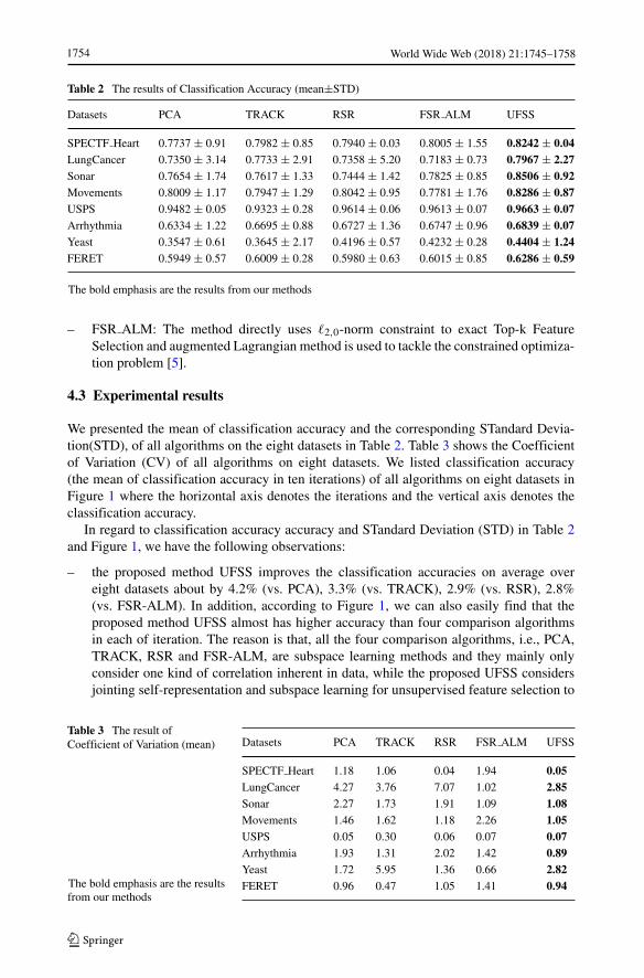
Table 2 The results of Classification Accuracy (mean±STD)
Datasets PCA TRACK RSR FSR ALM UFSS
SPECTF Heart 0.7737 ± 0.91 0.7982 ± 0.85 0.7940 ± 0.03 0.8005 ± 1.55 0.8242 ± 0.04LungCancer 0.7350 ± 3.14 0.7733 ± 2.91 0.7358 ± 5.20 0.7183 ± 0.73 0.7967 ± 2.27Sonar 0.7654 ± 1.74 0.7617 ± 1.33 0.7444 ± 1.42 0.7825 ± 0.85 0.8506 ± 0.92Movements 0.8009 ± 1.17 0.7947 ± 1.29 0.8042 ± 0.95 0.7781 ± 1.76 0.8286 ± 0.87USPS 0.9482 ± 0.05 0.9323 ± 0.28 0.9614 ± 0.06 0.9613 ± 0.07 0.9663 ± 0.07Arrhythmia 0.6334 ± 1.22 0.6695 ± 0.88 0.6727 ± 1.36 0.6747 ± 0.96 0.6839 ± 0.07Yeast 0.3547 ± 0.61 0.3645 ± 2.17 0.4196 ± 0.57 0.4232 ± 0.28 0.4404 ± 1.24FERET 0.5949 ± 0.57 0.6009 ± 0.28 0.5980 ± 0.63 0.6015 ± 0.85 0.6286 ± 0.59
The bold emphasis are the results from our methods
– FSR ALM: The method directly uses �2,0-norm constraint to exact Top-k FeatureSelection and augmented Lagrangian method is used to tackle the constrained optimiza-tion problem [5].
4.3 Experimental results
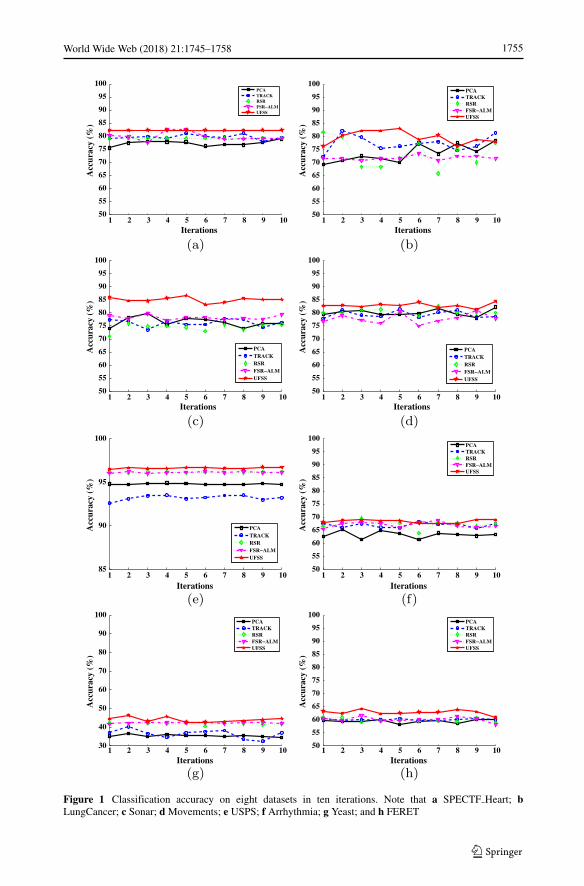
We presented the mean of classification accuracy and the corresponding STandard Devia-tion(STD), of all algorithms on the eight datasets in Table 2. Table 3 shows the Coefficientof Variation (CV) of all algorithms on eight datasets. We listed classification accuracy(the mean of classification accuracy in ten iterations) of all algorithms on eight datasets inFigure 1 where the horizontal axis denotes the iterations and the vertical axis denotes theclassification accuracy.
In regard to classification accuracy accuracy and STandard Deviation (STD) in Table 2and Figure 1, we have the following observations:
– the proposed method UFSS improves the classification accuracies on average overeight datasets about by 4.2% (vs. PCA), 3.3% (vs. TRACK), 2.9% (vs. RSR), 2.8%(vs. FSR-ALM). In addition, according to Figure 1, we can also easily find that theproposed method UFSS almost has higher accuracy than four comparison algorithmsin each of iteration. The reason is that, all the four comparison algorithms, i.e., PCA,TRACK, RSR and FSR-ALM, are subspace learning methods and they mainly onlyconsider one kind of correlation inherent in data, while the proposed UFSS considersjointing self-representation and subspace learning for unsupervised feature selection to
Table 3 The result ofCoefficient of Variation (mean) Datasets PCA TRACK RSR FSR ALM UFSS
SPECTF Heart 1.18 1.06 0.04 1.94 0.05LungCancer 4.27 3.76 7.07 1.02 2.85Sonar 2.27 1.73 1.91 1.09 1.08Movements 1.46 1.62 1.18 2.26 1.05USPS 0.05 0.30 0.06 0.07 0.07Arrhythmia 1.93 1.31 2.02 1.42 0.89Yeast 1.72 5.95 1.36 0.66 2.82FERET 0.96 0.47 1.05 1.41 0.94The bold emphasis are the results
from our methods
World Wide Web (2018) 21:1745–17581754
1 2 3 4 5 6 7 8 9 1050
55
60
65
70
75
80
85
90
95
100
Iterations
Accuracy
(%)
PCATRACKRSRFSR−ALMUFSS
1 2 3 4 5 6 7 8 9 1050
55
60
65
70
75
80
85
90
95
100
Iterations
Accuracy
(%)
PCATRACKRSRFSR−ALMUFSS
1 2 3 4 5 6 7 8 9 1050
55
60
65
70
75
80
85
90
95
100
Iterations
Accuracy
(%)
PCATRACKRSRFSR−ALMUFSS
1 2 3 4 5 6 7 8 9 1050
55
60
65
70
75
80
85
90
95
100
Iterations
Accuracy
(%)
PCATRACKRSRFSR−ALMUFSS
1 2 3 4 5 6 7 8 9 1085
90
95
100
Iterations
Accuracy
(%)
PCATRACKRSRFSR−ALMUFSS
1 2 3 4 5 6 7 8 9 1050
55
60
65
70
75
80
85
90
95
100
Iterations
Accuracy
(%)
PCATRACKRSRFSR−ALMUFSS
1 2 3 4 5 6 7 8 9 1030
40
50
60
70
80
90
100
Iterations
Accuracy
(%)
PCATRACKRSRFSR−ALMUFSS
1 2 3 4 5 6 7 8 9 1050
55
60
65
70
75
80
85
90
95
100
Iterations
Accuracy
(%)
PCATRACKRSRFSR−ALMUFSS
Figure 1 Classification accuracy on eight datasets in ten iterations. Note that a SPECTF Heart; bLungCancer; c Sonar; d Movements; e USPS; f Arrhythmia; g Yeast; and h FERET
World Wide Web (2018) 21:1745–1758 1755
obtain two kinds of correlation inherent in data. At the same time, the proposed UFSSintroduces a low-rank constraint to find the effective low-dimensional structures of thedata, which can guarantee to reduce the redundancy. Therefore, the UFSS can get betterperformances than other comparison algorithms.
– The proposed method UFSS outperforms PCA, TRACK, RSR and FSR-ALM muchbetter on LungCancer dataset, they are about 8.5%, 8.9%, 10.6% and 6.8%, respec-tively. The UFSS method absorbs the merits of both self-representation and LPP andintegrates them into a unified framework. Thus it can select the most discriminativefeatures and achieve the best classification accuracy.
– The proposed method UFSS has the least values of STandard Deviation (STD) com-pared with the comparison methods, it is less than others on average over eight datasetsabout by 0.28 (vs. PCA), 0.34 (vs. TRACK), 0.36 (vs. RSR), 0.05 (vs. FSR-ALM). Itshows that our proposed method is more stable than other comparison methods.
In regard to Coefficient of Variation (CV) in Table 3, we can observe that: the UFSS methodcannot always get the best performance on all datasets. For example, SPECTF Heart andFERET UPSS is not the least one. But in general, the proposed method UFSS achieved theleast coefficient of variation, i.e., 0.97, while other comparison methods are 1.39, 1.62, 1.47and 0.99 corresponding to PCA, TRACK,RSR and FSR-ALM, respectively. This showsthat the proposed algorithm UFSS is more robust than other comparison algorithms on thewhole.
5 Conclusion
In this paper, we have proposed an unsupervised feature selection method based on self-representation and subspace learning. We use all features to represent each feature. In otherwords, each feature is reconstructed by all the features. A Frobenius norm regularizer termto constrain the reconstruction coefficient matrix is used to overcome the over-fitting prob-lem and to select the most discriminative features. Also, we introduce Locality PreservingProjection (LPP) as a regularization term to maintain the local adjacent relation of the dataconstant when performing feature space transformation. Further, we consider applying alow-rank constraint to find the effective low-dimensional structures of the data. Experimentson real datasets have been conducted to compare the performances of the proposed methodand the other state-of-the-art methods. The experimental results showed that the proposedmethod UFSS outperformed other methods in terms of classification accuracy, standarddeviation and coefficient of variation.
In future, we consider improving the UFSS method for supervised feature selection.
Acknowledgments This work was in part supported by the Marsden Fund of New Zealand and the ChinaScholarship Council.
References
1. Bermejo, P., Gamez, J.A., Puerta, J.M.: A grasp algorithm for fast hybrid (filter-wrapper) feature subsetselection in high-dimensional datasets. Pattern Recogn. Lett. 32(5), 701–711 (2011)
2. Cai, D., He, X., Han, J.: Spectral regression: a unified approach for sparse subspace learning. In: IEEEICDM, pp. 73–82 (2007)
World Wide Web (2018) 21:1745–17581756
3. Cai, D., Zhang, C., He. X.: Unsupervised feature selection for multi-cluster data. In: ACM SIGKDD, pp.333–342 (2010)
4. Cai, X., Ding, C., Nie, F., Huang, H.: On the equivalent of low-rank linear regressions and lineardiscriminant analysis based regressions. In: ACM SIGKDD, pp. 1124–1132 (2013)
5. Cai, X., Nie, F., Huang, H.: Exact top-k feature selection via l2, 0-norm constraint. In: IJCAI, vol. 13,pp. 1240–1246 (2013)
6. Chang, X., Nie, F., Yang, Y., Huang, H.: A convex formulation for semi-supervised multi-label featureselection. In: AAAI, pp. 1171–1177 (2014)
7. Chen, X.-W., Zeng, X., van Alphen, D.: Multi-class feature selection for texture classification. PatternRecognit. Lett. 27(14), 1685–1691 (2006)
8. Gottumukkal, R., Asari, V.K.: An improved face recognition technique based on modular pca approach.Pattern Recognit. Lett. 25(4), 429–436 (2004)
9. Gu, Q., Li, Z., Han, J.: Joint feature selection and subspace learning. In: IJCAI, vol. 22(1), p. 129410. Hall, M.A., Smith, L.A.: Feature selection for machine learning: comparing a correlation-based filter
approach to the wrapper. In: FLAIRS, vol. 1999, pp. 235–239 (1999)11. He, X., Niyogi, P.: Locality preserving projections. In: NIPS, pp. 153–160 (2004)12. Hu, R., Zhu, X., Cheng, D., He, W., Yan, Y., Song, J., Zhang, S.: Graph self-representation method for
unsupervised feature selection. Neurocomputing 220, 130–137 (2017)13. Liu, R., Yang, N., Ding, X., Ma, L.: An unsupervised feature selection algorithm: Laplacian score
combined with distance-based entropy measure. In: IEEE IITA, vol. 3, pp. 65–68 (2009)14. Lu, C., Lin, Z., Yan, S.: Smoothed low rank and sparse matrix recovery by iteratively reweighted least
squares minimization. IEEE Trans. Image Process. 24(2), 646–654 (2015)15. Nikitidis, S., Tefas, A., Pitas, I.: Maximum margin projection subspace learning for visual data analysis.
IEEE Trans. Image Process. 23(10), 4413–4425 (2014)16. Qian, M., Zhai, C.: Robust unsupervised feature selection. In: IJCAI, pp. 1621–1627 (2013)17. Sebban, M., Nock, R.: A hybrid filter/wrapper approach of feature selection using information theory.
Pattern Recognit. 35(4), 835–846 (2002)18. Swiniarski, R.W., Skowron, A.: Rough set methods in feature selection and recognition. Pattern
Recognit. Lett. 24(6), 833–849 (2003)19. Tabakhi, S., Moradi, P., Akhlaghian, F.: An unsupervised feature selection algorithm based on ant colony
optimization. Eng. Appl. Artif. Intell. 32, 112–123 (2014)20. Velu, R., Reinsel, G.C.: Multivariate reduced-rank regression: theory and applications, vol. 136. Springer
Science Business Media, New York (2013)21. Wang, T., Qin, Z., Zhang, S., Zhang, C.: Cost-sensitive classification with inadequate labeled data. Inf.
Syst. 37(5), 508–516 (2012)22. Wang, H., Gao, Y., Shi, Y., Wang, R.: Group-based alternating direction method of multipliers for dis-
tributed linear classification. In: IEEE transactions on cybernetics. https://doi.org/10.1109/TCYB.2016.2570808, pp. 1–15 (2016)
23. Wu, J., Long, J., Liu, M.: Evolving rbf neural networks for rainfall prediction using hybrid particle swarmoptimization and genetic algorithm. Neurocomputing 148, 136–142 (2015)
24. Yan, S., Xu, D., Zhang, B., Zhang, H.-J., Yang, Q., Lin, S.: Graph embedding and extensions: a generalframework for dimensionality reduction. IEEE Trans. Pattern Anal. Mach. Intell. 29(1), 40–51 (2007)
25. Yi, P., Song, A., Guo, J., Wang, R.: Regularization feature selection projection twin support vectormachine via exterior penalty. Neural Comput. Appl. 1–15 (2016)
26. Zhang, S.: Shell-neighbor method and its application in missing data imputation. Appl. Intell. 35(1),123–133 (2011)
27. Zhang, S., Jin, Z., Zhu, X.: Missing data imputation by utilizing information within incomplete instances.J. Syst. Softw. 84(3), 452–459 (2011)
28. Zhang, S., Cheng, D., Zong, M., Gao, L.: Self-representation nearest neighbor search for classification.Neurocomputing 195, 137–142 (2016)
29. Zhang, S., Li, X., Zong, M., Zhu, X., Cheng, D.: Learning k for knn classification. ACM Trans. Intell.Syst. Technol. 8(3), 43 (2017)
30. Zhang, S., Li, X., Zong, M., Zhu, X., Wang, R.: Efficient knn classification with different numbers ofnearest neighbors. IEEE Trans. Neural Netw. Learn. Syst. 1–12 https://doi.org/10.1109/TNNLS.2017.2673241 (2017)
31. Zhu, X., Zhang, S., Jin, Z., Zhang, Z., Xu, Z.: Missing value estimation for mixed-attribute data sets.IEEE Trans. Knowl. Data Eng. 23(1), 110–121 (2011)
32. Zhu, X., Zhang, L., Huang, Z.: A sparse embedding and least variance encoding approach to hashing.IEEE Trans. Image Process. 23(9), 3737–3750 (2014)
World Wide Web (2018) 21:1745–1758 1757

33. Zhu, P., Zuo, W., Zhang, L., Hu, Q., Shiu, S.C.: Unsupervised feature selection by regularized self-representation. Pattern Recognit. 48(2), 438–446 (2015)
34. Zhu, X., Li, X., Zhang, S.: Block-row sparse multiview multilabel learning for image classification.IEEE Trans. Cybern. 46(2), 450–461 (2016)
35. Zhu, X., Suk, H.-I., Lee, S.-W., Shen, D.: Subspace regularized sparse multitask learning for multiclassneurodegenerative disease identification. IEEE Trans. Biomed. Eng. 63(3), 607–618 (2016)
36. Zhu, X., Li, X., Zhang, S., Ju, C., Wu, X.: Robust joint graph sparse coding for unsupervised spectralfeature selection. IEEE Trans. Neural Netw. Learn. Syst. 28(6), 1263–1275 (2017)
37. Zhu, X., Li, X., Zhang, S., Xu, Z., Yu, L., Wang, C.: Graph pca hashing for similarity search. IEEETrans. Multimed. 19(9), 2033–2044 (2017)
38. Zhu, X., Suk, H., Wang, L., Lee, S., Shen, D.: A novel relational regularization feature selection methodfor joint regression and classification in AD diagnosis. Med. Image Anal. 38, 205–214 (2017)
39. Zou, H., Hastie, T., Tibshirani, R.: Sparse principal component analysis. J. Comput. Graph. Stat. 15(2),265–286 (2006)
World Wide Web (2018) 21:1745–17581758