Journal of Cleaner Production - MIT Concrete …...Journal of Cleaner Production xxx (2016) 1e9 Please cite this article in press as: Louhghalam, A., et al., Carbon management of infrastructure

lable at ScienceDirect

Journal of Cleaner Production xxx (2016) 1e9

Contents lists avai

Journal of Cleaner Production

journal homepage: www.elsevier .com/locate/ jc lepro

Carbon management of infrastructure performance: Integrated bigdata analytics and pavement-vehicle-interactions

Arghavan Louhghalam, Mehdi Akbarian, Franz-Josef Ulm*

Massachusetts Institute of Technology, Cambridge, MA, United States

a r t i c l e i n f o

Article history:Received 25 October 2015Received in revised form5 June 2016Accepted 30 June 2016Available online xxx

Keywords:Pavement-vehicle-interactionGreenhouse gas emissionsNetwork analysisPower-law distributionBig data analytics

* Corresponding author.E-mail address: [email protected] (F.-J. Ulm).

http://dx.doi.org/10.1016/j.jclepro.2016.06.1980959-6526/© 2016 Elsevier Ltd. All rights reserved.

Please cite this article in press as: Louhghalapavement-vehicle-interactions, Journal of C

a b s t r a c t

As a crucial part of the transportation system, roadway network provides mobility to the society and isvital for the economy. At the same time it contributes significantly to the environmental footprint duringits construction, operation and maintenance. Hence, the sustainable development of our Nation'sroadway system requires quantitative means to link infrastructure performance to lifecycle energy useand greenhouse gas emissions. Recent developments in mechanistic models of roughness- anddeflection-induced pavement-vehicle interaction aim at providing such engineering estimates. Herein, itis demonstrated that these models when implemented at a network scale are a powerful basis for bigdata analytics of excess-energy consumption and carbon dioxide emissions by integrating spatially andtemporally varying road conditions, pavement properties, traffic loads and climatic conditions. A novelranking algorithm is proposed, that allows upscaling of the local carbon dioxide emissions due topavement vehicle interaction to the size of state-wide or national sustainability goals. Implemented for5157 lane-miles of the interstate highway system in the State of Virginia, sections contributing signifi-cantly to carbon dioxide emissions are identified. It is shown that the proposed ranking algorithm basedon the inferred emission that exhibits a power-law distribution, provides the shortest path for green-house gas emissions savings per maintenance at network scale. That is, maintaining a few lane milesallows for a significant synergetic improvement of both infrastructure performance and environmentalimpact of the interstate network and helps transportation agencies in making economic and environ-mentally sustainable decisions.

© 2016 Elsevier Ltd. All rights reserved.

1. Introduction

Accounting for 28% of the total United States greenhouse gas(GHG) emissions, the transportation sector, was the second largestcontributor to the GHG emissions in 2012 (EPA, 2012). With morethan four millionmiles of public roads, andwith generation of 6526million metric tons of Carbon Dioxide (CO2) and total fuel con-sumption of around 168 billion gallons (FHWA, 2012) the USroadway network has a significant impact on the environment.Pavement condition, design and characteristics affect vehicle fuelconsumption and the relating CO2 emissions (Gyenes and Mitchell,1994; Chatti and Zaabar, 2012). Thus maintaining the Nation'sroadway network at good conditions, besides enhancing roadwaysperformance, results in a more sustainable transportation system.However, by some estimates (U.S. Department of Transportation,

m, A., et al., Carbon managemleaner Production (2016), htt

Federal Transit Administration, 2013) maintaining the nationalhighways at their current condition requires spending annually $95to $109 billion during 2014 and 2020 respectively. The cost wouldincrease to $161.7 and $184.2 billion to improve the condition.Given the limited financial resources of federal and state trans-portation agencies for road maintenance along with the initiativesfor sustainable development, it is critical to develop fast and ac-curate frameworks for identifying the roads with higher environ-mental footprint, and to establish strategies for selecting pavementsections for maintenance that maximize investment returns interms of the total network-level environmental impact.

While the environmental impact of material production(Huntzinger and Eatmon, 2009) and pavement construction andmaintenance phases (Turk et al., 2016; Huang et al., 2009;Fern�andez-S�anchez et al., 2015) are widely studied in Life CycleAssessment (LCA) of pavements, the use-phase impact is generallyomitted in most of pavement LCA tools (Santero et al., 2011).Considering the fact that the impact of use phase for high volume

ent of infrastructure performance: Integrated big data analytics andp://dx.doi.org/10.1016/j.jclepro.2016.06.198

Delta:1_given name

Delta:1_surname

Delta:1_given name

mailto:[email protected]

www.sciencedirect.com/science/journal/09596526

http://www.elsevier.com/locate/jclepro

http://dx.doi.org/10.1016/j.jclepro.2016.06.198



A. Louhghalam et al. / Journal of Cleaner Production xxx (2016) 1e92

traffic roads is significant and can surpass other embodied emis-sions (Wang et al., 2012; Araújo et al., 2014) the need to close thisgap is evident.

Rolling resistance e due to pavement roughness, texture(Sandberg et al., 2011) and deflection e can contribute 15%e50% tothe total vehicle fuel consumption, depending on vehicle speed(Beuving et al., 2004), and is one of the main factors in pavement'suse-phase environmental footprint. Although small for a singlevehicle, the aggregated impact for pavement sections with hightraffic volume can exceed other factors contributing to the lifecyclefootprint of pavements (Wang et al., 2012; Noshadravan et al.,2013). Pavement-vehicle-interaction (PVI) models quantitativelyassess this footprint by taking into account the impact of differentpavement characteristics and designs, and existing climatic andtraffic conditions in the roadway network, on the energy dissipa-tion and the ensuing excess fuel consumption. These models arethus important components in evaluating pavement sustainabilityperformance. Furthermore, when combined with information atthe network level, they can serve as a means to guide carbonmanagement policies aiming at reduction of CO2 emissions inroadway networks.

Herein, an approach is proposed that integrates roughness- anddeflection-induced PVI models with various databases, which areavailable to transportation agencies, to identify pavement sectionswith the greatest potential for CO2 emissions reduction at thenetwork scale. By way of example, using big data analytics, thespatial and temporal variation of CO2 emissions in the network ofVirginia interstate highways due to the change in road conditionand design is investigated, while considering variation in climaticconditions and traffic loads. In addition, a ranking algorithm fornetwork maintenance strategy is proposed that results in bothmaximum reduction of use-phase CO2 emissions at the networkscale and improvement of infrastructure performancesimultaneously.

2. Pavement-vehicle-interaction (PVI) models

The first step in development of a framework for an optimalmaintenance strategy is to quantify the impact of pavement char-acteristics, environmental conditions and vehicle properties onexcess vehicle fuel consumption and the corresponding CO2 emis-sion. While empirical investigations highlight the existence ofcorrelation between fuel consumption and pavement structural(Taylor, 2002; Taylor and Patten, 2006; Gsch€osser and Wallbaum,2013), and surface properties (Taylor et al., 2000; Zaniewski et al.,1982), until recently the link between several pavement charac-teristics and vehicle fuel consumption was missing. Newly devel-oped deflection-induced (Pouget et al., 2011; Louhghalam et al.,2013) and roughness-induced PVI models (Chatti and Zaabar,2012; Velinsky and White, 1980; Louhghalam et al., 2015) aim atclosing this gap by establishing a link between mechanical prop-erties of pavements and vehicle fuel consumption.

The underlying concept behind the PVI models is that tomaintain a constant speed, the dissipated energy due to rollingresistance must be compensated by extra engine power which re-sults in excess vehicle fuel consumption and GHG emissions.Deflection- and roughness-induced PVI models respectively ac-count for the dissipation of energy in pavement material andvehicle suspension system. The impact of pavement texture onvehicle fuel consumption has not taken into account in the networkanalysis due to lack of available information.

2.1. Deflection-induced PVI

The recently developed deflection-induced PVI (Louhghalam

Please cite this article in press as: Louhghalam, A., et al., Carbon managempavement-vehicle-interactions, Journal of Cleaner Production (2016), htt

et al., 2013) provide a means to quantitatively assess the impactof pavement characteristics (e.g., subgrade modulus, pavementthickness, stiffness and viscosity) and climatic conditions onvehicle fuel consumption.

The key underlying principal behind deflection-induced PVI is:the energy dissipated within pavement material due to its visco-elasticity must be compensated by an external energy source,leading to excess fuel consumption. Using the first and second lawsof thermodynamics, it is shown that the dissipated energy perdistance travelled dε is directly related to the slope underneath thewheel in a moving coordinate system that is attached to andtraveling with the tire with speed V, i.e. dE ¼ �Pdw=dX, where P isthe axle load, dw/dX is the average slope at tire-pavement trajectoryin the moving coordinate system X ¼ x�Vt, with x and t denotingcoordinates of space and time in a fixed coordinate system(Louhghalam et al., 2013). It is worth noting that in this coordinatesystem, the maximum deflection of an elastic material subjected toa moving tire occurs exactly under the tire. That means the averageslope, thus the deflection-induced energy dissipation is zero for anelastic material, which is in agreement with the laws ofthermodynamics.

The pavement is modeled as an infinite viscoelastic beam on anelastic foundation subjected to an axle load traveling with a con-stant speed V in steady-state condition. The constitutive relationbetween stress s and strain ε of the viscoelastic material isdescribed by a Maxwell model, ðsþ t _sÞ=E ¼ t _ε, with the Young'smodulus E and relaxation time t ¼ h/E, where h is the materialviscosity and the superposed dot denotes time derivative. The dif-ferential equation of beam's displacement w in the moving coor-dinate system:

Eh3

12d4wdX4 þmV2d

2wdX2 þ kw ¼ p (1)

with h pavement thickness, k subgrade stiffness andm surfacemassdensity, is solved in the frequency domain, by using the elastic-viscoelastic correspondence principle (Christensen, 1982). Theaverage slope at the tire-pavement trajectory and ultimately theenergy dissipation within the material is evaluated (seeLouhghalam et al. (2013) for detailed solution).

Substituting this involving mathematical procedure with anaccurate and computationally efficient expression is the nextcrucial task in developing models that are practical for big dataanalytics of network-scale analysis. This is achieved by rationalizingthe problem through a dimensional analysis of physical quantitiesinvolved in the dissipated energy per distance travelled, dε, namelysubgrade stiffness k, pavement stiffness E, thickness h, width b, andrelaxation time t, as well as temperature T, vehicle axle load P andspeed V. The analysis allows for further reduction of the problem toa 2-parameter relation between the dimensionless dissipation P ¼dE Vbkl2s =VcrP2 and dimensionless vehicle speed V/Vcr and relaxa-tion time tVcr/ls using BuckinghamP-theorem Buckingham (1914):

P ¼ dE Vbkl2sVcrP2

¼ F

�P1 ¼ Vcr

V;P2 ¼ tVcr

ls

�(2)

with Vcr ¼ lsk/m, and ls ¼ ðEh3=12kÞ1=4 the Winkler length of thebeam. The analysis above also provides scaling relationship of en-ergy dissipation with different pavement mechanical properties,vehicle characteristics and temperature:

dE fðVtÞ�1 � P2 � E�1=4 � h�3=4 � k�1=4 (3)

Note that the functional relation F in expression (2) cannot beevaluated using the P-theorem and must be determined by


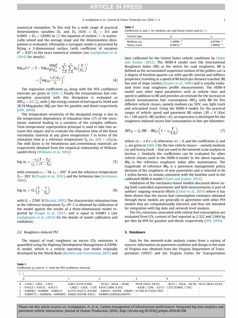
Table 2Coefficients bc and gc for medium cars and heavy trucks used in (7).

Vehicle type bc gc

Medium car 1.2098e�3 2.8190e�2

Heavy truck 4.4461e�3 1.9899e�2

A. Louhghalam et al. / Journal of Cleaner Production xxx (2016) 1e9 3

numerical simulation. To this end for a wide range of practicaldimensionless variables P1 and P2 (0.03 < P1 < 0.5 and0.0001 < P2 < 12000) in (2) the equation of motion (1) is numer-ically solved and the average slope and the dimensionless dissi-pations is evaluated. Ultimately a surrogate model is presented byfitting a 2-dimensional surface (with coefficient of variationR2 ¼ 0.97) to the exact numerical solution (see Louhghalam et al.(2014) for details):

log10dE ¼ 3� log10Vbkl2sP2Vcr

þX5i¼0

X3j¼0

pij

�VVcr

�i

��log10

tðTÞVcr

ls

�j

(4)

The regression coefficients pij along with the 95% confidenceintervals are given in Table 1. Finally the instantaneous fuel con-sumption associated with this dissipation is evaluated asdIFCD ¼ dE =zf , with zf the energy content of fuel equal to 34.84 and38.74 Megajoules (MJ) per liter for gasoline and diesel respectively(EPA, 2004).

The temperature sensitivity of the dissipated energy is due tothe temperature dependency of relaxation time t(T) of the visco-elastic material leading to a variation of the complex stiffness.Time-temperature superposition principal is used to take into ac-count this impact and to evaluate the relaxation time of the linearviscoelastic material at any given temperature T in terms of therelaxation time at a reference temperature T0, i.e., t(T) ¼ t(T0) aT.The shift factor aT for bituminous and cementitious materials arerespectively obtained from the empirical relationship of William-Landel-Ferry (Williams et al., 1955):

log aT ¼ �c1ðT � T0Þc2 þ ðT � T0Þ

(5)

with constants c1 ¼ 34, c2 ¼ 203+ K and the reference temperatureT0 ¼ 283� K (Pouget et al., 2011), and the Arrhenius law (Arrhenius,1889):

log aT ¼ Uc

�1T� 1T0

�(6)

with Uc ¼ 2700� K (Bazant, 1995). The characteristic relaxation timeat the reference temperature T0¼10� C is obtained by calibration ofthe model against the results of a three-dimensional model re-ported by Pouget et al. (2011) and is equal to 0.0083 s (seeLouhghalam et al. (2014) for the details of model calibration andvalidation).

2.2. Roughness-induced PVI

The impact of road roughness on excess CO2 emissions isquantified using the Highway Development Management-4 (HDM-4) model, which is a vehicle operating cost model originallydeveloped by the World Bank (Bennett and Greenwood, 2001) and

Table 1Coefficients pij used in (4) with the 95% confidence intervals.

j i

0 1 2

0 �1.918 (�1.922, �1.915) 4.487 (4.379, 4.596) �19.54 (�20.64, �181 �0.4123 (�0.4135, �0.4111) �1.802 (�1.824, �1.78) 4.014 (3.864, 4.163)2 �0.06942 (�0.06969, �0.06915) 0.2153 (0.2111, 0.2194) �0.8618 (�0.8794, �3 �0.009575 (�0.009656,�0.009495) 0.0203 (0.0196, 0.021) 0.04669 (0.04542,0.0


later calibrated for the United States vehicle conditions by Chattiand Zaabar (2012). The HDM-4 model uses the InternationalRoughness Index (IRI) as the metric for road roughness. IRI isdefined as the accumulated suspension motion of the golden-car (a2-degree of freedom quarter-car with specific inertial and stiffnessproperties) traveling at a speed of 80 km/h per distance traveled. IRIhas unit of slope (m/km) (Sayers et al., 1986) and is usually evalu-ated from road roughness profile measurements. The HDM-4model uses other input parameters such as vehicle class andspeed in addition to IRI and provides an estimate for the increase invehicle instantaneous fuel consumption dIFCR with IRI for fivedifferent vehicle classes, namely medium car, SUV, van, light truckand articulated truck. Using the HDM-4 model, for the practicalranges of vehicle speed and pavement IRI values (30 < V (Km/h) < 130 and 0< IRI (m/Km) <6), an expression is developed for theroughness-induced excess fuel consumption in liter per kilometer:

dIFCR ¼ bchIRI� IRI0i�1þ gc

V3:6

�(7)

where ⟨x⟩ ¼ x if x > 0, otherwise ⟨x⟩ ¼ 0, and the coefficients bc andgc are given in Table 2 for the two vehicle classese namelymediumcar and heavy truck e that are used in the network-scale analysis inSection 4. Similarly the coefficients can be evaluated for othervehicle classes used in the HDM-4 model. In the above equation,IRI0 is the reference roughness index after maintenance. Themagnitude of reference IRI0 is a pavement management policydecision of the roughness of new pavements and is selected to be1 m/km herein, to remain consistent with the baseline used in thecalibrated HDM-4 model (Chatti and Zaabar, 2012).

Validation of the mechanics-based models discussed above us-ing both controlled experiments and field measurements is part ofauthors' ongoing research efforts (Coleri et al., 2015) where it hasbeen shown that the excess fuel consumption estimates obtainedthrough these models are generally in agreement with other PVImodels that are computationally intensive and thus not intendedfor integration with big data and network level analysis.

The CO2 emissions associated with vehicle fuel consumption areevaluated from CO2 content of fuel reported as 2.322 and 2.664 kgper liter by EPA for gasoline and diesel, respectively (EPA, 2005).

3. Databases

Data for the network-scale analysis comes from a variety ofsources. Information on pavement condition and design in the stateof Virginia was obtained from the Virginia Department of Trans-portation (VDOT) and the Virginia Center for Transportation

3 4 5

.44) 59.58 (54.61, 64.55) �92.51 (�102.6, �82.39) 56.23 (48.63, 63.83)�4.628 (�5.04, �4.217) 1.375 (0.9895, 1.761) e

0.8441) 0.7344 (0.7124,0.7563) e e

4797) e e e


Table 3Pavement types and their corresponding length in Virginia interstate highways.

VA labels Pavement type Lane-mile Center-mile

BIT Asphalt (AC) 3131 1416JRCP Concrete (PCC) 360 119CRCP Concrete (PCC) 382 143BOJ Composite (CMP) 854 294BOC Composite (CMP) 430 183


Innovation and Research (VCTIR). The data consists of structural,material and surface properties of pavement sections along withtheir mileposts for five pavement types comprising the interstatehighways, namely Bituminous (BIT), Joint Reinforced ConcretePavement (JRCP), Continuous Reinforced Concrete Pavement(CRCP), Bituminous over JRCP (BOJ) and Bituminous over CRCP(BOC). The corresponding length of each pavement type in thenetwork of Virginia interstate highways is summarized in Table 3.For each pavement section the dataset includes section identifier,milepost, pavement thickness, pavement and subgrade modulialong with measured IRI values. Pavement and subgrade moduliprovided by Virginia Center for Transportation Research are ob-tained by back-calculation using the results of Falling WeightDeflectometer (FWD) testing which has been implemented at thenetwork level by VDOT (Galal et al., 2007; Diefenderfer, 2010). Inaddition to these pavement properties, the data set also includesthe annual average daily traffic (AADT) and truck traffic (AADTT) forseven years (2007e2013) for the entire interstate system. To matchthis data with its geographical location via Geographical Informa-tion System (GIS) (ArcGIS 10.2.2), the basemap of VA interstatehighways from Federal Highway Administration's National Plan-ning Network (NHPN, 2013) is used along with pavement sectionmileposts (see the Supporting information for the maps of IRI,pavement type and traffic).

The temperature data is obtained from the dataset of NationalOceanic and Atmospheric Administration (NOAA) in the form ofaverage monthly temperatures for six different climatic regionscomprising the state of Virginia. Pavementmileposts enable findingthe climatic regions and thus temperature variations for all

Fig. 1. Flow of network analysis; the inputs and the outp


pavement sections in the interstate highway network.The information on vehicle speed in VA interstate highways is

inferred from the Weigh In Motion (WIM) data provided by VDOT.The dataset consists of axle weight, gross vehicle weight andvehicle speed. The measured vehicle speeds are used to estimatespeed probability density function (PDF) in Virginia interstatesystem. It is observed that the vehicle speeds in the network followa Gaussian distribution with a mean value of 103.93 km/h and astandard deviation of 7.52. The Gaussian PDF is later used for aMonte-Carlo simulation in the network-scale analysis.

4. Network-scale analysis

Fast and straightforward implementation of PVI models pro-vides a convenient tool to upscale pavement section emissions tothe network scale environmental impact. To this end, the compo-nent level PVI models are integrated with the datasets describedabove to perform a network-level analysis. The flowchart of thenetwork analysis illustrated in Fig. 1 summarizes how the data setsdescribed in the previous section provide the inputs to the PVImodels. The indicator of pavement roughness (IRI) and vehiclespeed are the inputs to the roughness-induced PVI model (Equation(7) and Table 2), whereas pavement structural and material prop-erties, temperature and vehicle speeds are used to estimate thedeflection-induced energy dissipation and the relating CO2 emis-sions (Equation (4) and Table 1).

To take into account the uncertainty associated with vehiclespeed and its impact on the excess fuel consumption due topavement roughness and deflection, a Monte-Carlo Simulation isperformed. For each road section inverse transformation samplingis used to generate 1000 samples of vehicle speed according to theGaussian PDF obtained from the WIM data (i.e. a set of 1000 in-dependent uniformly distributed random variables, U ¼ u[0,1] isgenerated and the inverse of the Gaussian cumulative distributionfunction (CDF) at U, X ¼ F�1

V ðUÞ, is calculated) and evaluate the 95percentile of the CO2 emissions.

The structural and material data for this study were availablefrom the Virginia Department of Transportation. However for caseswhere data is not available, an approach similar to the above can be

ut of deflection- and roughness-induced PVI models.


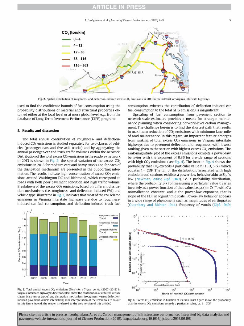
Fig. 2. Spatial distribution of roughness- and deflection-induced excess CO2 emissions in 2013 in the network of Virginia interstate highways.


used to find the confidence bounds of fuel consumption using theprobability distributions of material and structural properties ob-tained either at the local level or at more global level, e.g., from thedatabase of Long Term Pavement Performance (LTPP) program.

5. Results and discussion

The total annual contribution of roughness- and deflection-induced CO2 emissions is studied separately for two classes of vehi-cles (passenger cars and five-axle trucks) and by aggregating theannual passenger-car and truck traffic volumes within the network.Distributionof the total excessCO2 emissions in the roadwaynetworkin 2013 is shown in Fig. 2; the spatial variation of the excess CO2emissions in 2013 for medium cars and heavy trucks and for each ofthe dissipation mechanism are presented in the Supporting infor-mation. The results indicate high-concentration of excess CO2 emis-sions around Washington DC and Richmond, which correspond toroads with both poor pavement condition and high traffic volume.Breakdown of the excess CO2 emissions, based on different dissipa-tion mechanisms (i.e. roughness- and deflection-induced PVI) andvehicle type, illustrated in Fig. 3, indicates thatmost of the PVI relatedemissions in Virginia interstate highways are due to roughness-induced car fuel consumption, and deflection-induced truck fuel

Fig. 3. Total annual excess CO2 emissions (Tons) for a 7-year period (2007e2013) inVirginia interstate highways; different colors show the contribution of different vehicleclasses (cars versus trucks) and dissipation mechanisms (roughness- versus deflection-induced pavement vehicle interaction). (For interpretation of the references to colourin this figure legend, the reader is referred to the web version of this article.)


consumption, whereas the contribution of deflection-induced carfuel consumption to the total GHG emissions is insignificant.

Upscaling of fuel consumption from pavement section tonetwork-scale estimates provides a means for strategic mainte-nance planning when considering network-level carbon manage-ment. The challenge herein is to find the shortest path that resultsin maximum reduction of CO2 emissions with minimum lane-mileof road maintenance. In this regard, an important feature emergesfrom ranking of total excess CO2 emissions in Virginia interstatehighways due to pavement deflection and roughness, with lowestranking given to the sectionwith highest excess CO2 emissions. Therank-magnitude plot of the excess emissions exhibits a power-lawbehavior with the exponent of 0.36 for a wide range of sectionswith high CO2 emissions (see Fig. 4). The inset in Fig. 4 shows theprobability that CO2 exceeds a particular value x, P(CO2 > x), whichequates 1� CDF. The tail of the distribution, associated with highemission road sections, exhibits a power-law behavior akin to Zipf'slaw (Newman, 2005; Zipf, 1949), i.e. a probability distribution,where the probability p(x) of measuring a particular value x variesinversely as a power function of that value, i.e. p(x) ¼ Cx�a, with C anormalization constant, and a the power-law exponent, that isslope of the PDF in logarithmic scale. Power-law behavior appearsin a wide range of phenomena such as magnitudes of earthquakes(Gutenberg and Richter, 1944), frequency of words (Zipf, 1949;

Fig. 4. Excess CO2 emissions in function of its rank. Inset figure shows the probabilitythat the excess CO2 emissions exceeds a particular value, i.e. 1� CDF.


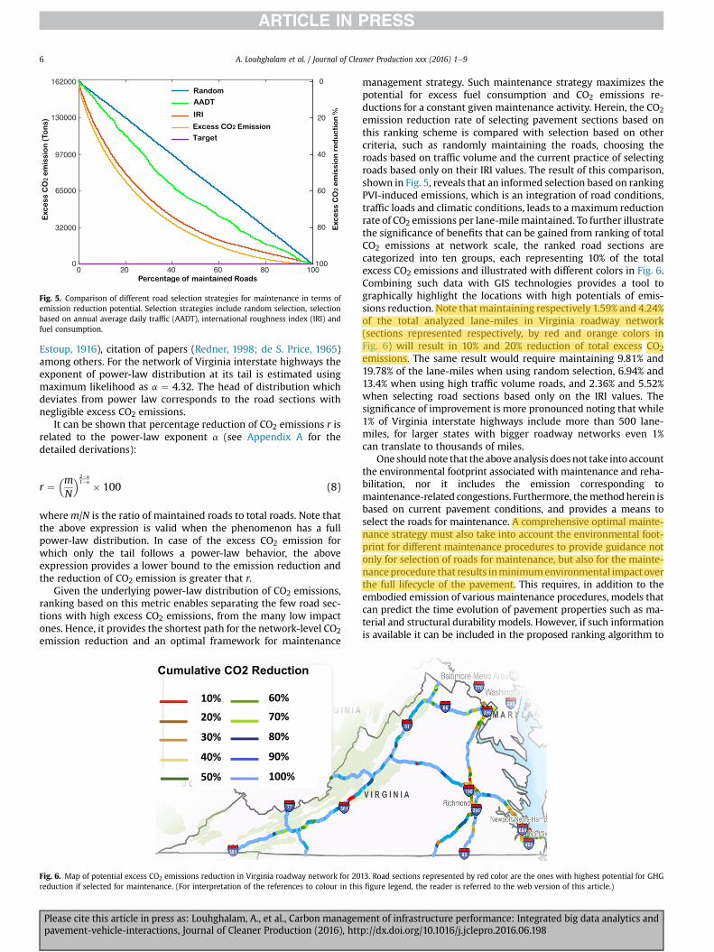
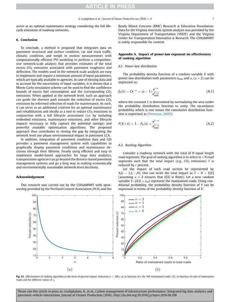
Fig. 5. Comparison of different road selection strategies for maintenance in terms ofemission reduction potential. Selection strategies include random selection, selectionbased on annual average daily traffic (AADT), international roughness index (IRI) andfuel consumption.


Estoup, 1916), citation of papers (Redner, 1998; de S. Price, 1965)among others. For the network of Virginia interstate highways theexponent of power-law distribution at its tail is estimated usingmaximum likelihood as a ¼ 4.32. The head of distribution whichdeviates from power law corresponds to the road sections withnegligible excess CO2 emissions.

It can be shown that percentage reduction of CO2 emissions r isrelated to the power-law exponent a (see Appendix A for thedetailed derivations):

r ¼�mN

�2�a1�a � 100 (8)

wherem/N is the ratio of maintained roads to total roads. Note thatthe above expression is valid when the phenomenon has a fullpower-law distribution. In case of the excess CO2 emission forwhich only the tail follows a power-law behavior, the aboveexpression provides a lower bound to the emission reduction andthe reduction of CO2 emission is greater that r.

Given the underlying power-law distribution of CO2 emissions,ranking based on this metric enables separating the few road sec-tions with high excess CO2 emissions, from the many low impactones. Hence, it provides the shortest path for the network-level CO2emission reduction and an optimal framework for maintenance

Fig. 6. Map of potential excess CO2 emissions reduction in Virginia roadway network for 20reduction if selected for maintenance. (For interpretation of the references to colour in thi


management strategy. Such maintenance strategy maximizes thepotential for excess fuel consumption and CO2 emissions re-ductions for a constant given maintenance activity. Herein, the CO2emission reduction rate of selecting pavement sections based onthis ranking scheme is compared with selection based on othercriteria, such as randomly maintaining the roads, choosing theroads based on traffic volume and the current practice of selectingroads based only on their IRI values. The result of this comparison,shown in Fig. 5, reveals that an informed selection based on rankingPVI-induced emissions, which is an integration of road conditions,traffic loads and climatic conditions, leads to a maximum reductionrate of CO2 emissions per lane-milemaintained. To further illustratethe significance of benefits that can be gained from ranking of totalCO2 emissions at network scale, the ranked road sections arecategorized into ten groups, each representing 10% of the totalexcess CO2 emissions and illustrated with different colors in Fig. 6.Combining such data with GIS technologies provides a tool tographically highlight the locations with high potentials of emis-sions reduction. Note that maintaining respectively 1.59% and 4.24%of the total analyzed lane-miles in Virginia roadway network(sections represented respectively, by red and orange colors inFig. 6) will result in 10% and 20% reduction of total excess CO2emissions. The same result would require maintaining 9.81% and19.78% of the lane-miles when using random selection, 6.94% and13.4% when using high traffic volume roads, and 2.36% and 5.52%when selecting road sections based only on the IRI values. Thesignificance of improvement is more pronounced noting that while1% of Virginia interstate highways include more than 500 lane-miles, for larger states with bigger roadway networks even 1%can translate to thousands of miles.

One shouldnote that the above analysis does not take into accountthe environmental footprint associated with maintenance and reha-bilitation, nor it includes the emission corresponding tomaintenance-related congestions. Furthermore, themethodherein isbased on current pavement conditions, and provides a means toselect the roads for maintenance. A comprehensive optimal mainte-nance strategy must also take into account the environmental foot-print for different maintenance procedures to provide guidance notonly for selection of roads for maintenance, but also for the mainte-nanceprocedure that results inminimumenvironmental impact overthe full lifecycle of the pavement. This requires, in addition to theembodied emission of various maintenance procedures, models thatcan predict the time evolution of pavement properties such as ma-terial and structural durability models. However, if such informationis available it can be included in the proposed ranking algorithm to

13. Road sections represented by red color are the ones with highest potential for GHGs figure legend, the reader is referred to the web version of this article.)


jwmack

Highlight

jwmack

Highlight


arrive at an optimal maintenance strategy considering the full life-cycle emissions of roadway networks.

6. Conclusion

To conclude, a method is proposed that integrates data onpavement structural and surface condition, car and truck traffic,climatic condition, and weigh in motion measurements withcomputationally efficient PVI modeling to perform a comprehen-sive network-scale analysis that provides estimates of the totalexcess CO2 emissions associated with pavement roughness anddeflection. The models used in the network-scale analysis are easyto implement and require a minimum amount of input parameters,which are typically available to agencies. In case of missing data andto account for the uncertainty of input variables, it is shown that aMonte Carlo simulation scheme can be used to find the confidencebounds of excess fuel consumption and the corresponding CO2emissions. When applied at the network level, such an approachcan guide the shortest path towards the reduction of excess CO2emissions by informed selection of roads for maintenance. As such,it can serve as an additional criterion for an optimal maintenanceand rehabilitation and ideally as a tool to reduce CO2 emissions inconjunction with a full lifecycle assessment (i.e. by includingembodied emissions, maintenance emissions, and other lifecycleimpacts necessary to fully capture the potential savings) andpowerful available optimization algorithms. The proposedapproach thus contributes to closing the gap by integrating thenetwork level use-phase environmental impact in pavement LCA.

In addition, integration of pavement condition data and GISprovides a pavement management system with capabilities tographically display pavement conditions and maintenance de-cisions through their lifetime. Finally using efficient and easy toimplement model-based approaches for large data analytics,transportation agencies can go beyond the distress-based pavementmanagement systems and go a long way in making economicallyand environmentally sustainable network-level decisions.

Acknowledgement

This research was carried out by the CSHub@MIT with spon-sorship provided by the Portland Cement Association (PCA) and the

Fig. A1. Effectiveness of ranking algorithm in the form of percent impact reduction (r � 100roads and for different values of a.


Ready Mixed Concrete (RMC) Research & Education Foundation.Data for the Virginia interstate system analysis was provided by theVirginia Department of Transportation (VDOT) and the VirginiaCenter for Transportation Innovation & Research. The CSHub@MITis solely responsible for content.

Appendix A. Impact of power-law exponent on effectivenessof ranking algorithm

A.1. Power-law distribution

The probability density function of a random variable X withpower-law distribution with parameters xmin and a, (a > 2) can beexpressed as:

fXðxÞ ¼ Cx�a ¼ ða� 1Þ x�a

x1�amin

(A.1)

where the constant C is determined by normalizing the area underthe probability distribution function to unity. The exceedanceprobability which is one minus the cumulative distribution func-tion is expressed as (Newman, 2005):

PðX > xÞ ¼ 1� FXðxÞ ¼x1�a

x1�amin

(A.2)

A.2. Ranking Algorithm

Consider a roadway network with the total of N equal lengthroad segments. The goal of ranking algorithm is to selectm < N roadsegments such that the total impact (e.g., CO2 emissions) T isreduced by r percent.

Let the impact of each road section be represented byXi{i ¼ 1,2,/,N}. One can write the total impact as T ¼ N � E[X](assuming a > 2 ensures that E[X] is finite). Let a new randomvariable Y¼{XjX > xm} represent the maintained roads. Using con-ditional probability, the probability density function of Y can beexpressed in terms of the probability density function of X:

), (a) in function of a for 10% maintained roads; (b): in function of ratio of maintained



fY ðyÞ ¼fXðyÞZ ∞

xmfXðxÞdx

(A.3)

Thus the expected value of Y is readily evaluated:

E½Y � ¼ 1Z ∞

xmfXðxÞdx

Z∞

xm

yfXðyÞdy (A.4)

To determine the effectiveness of ranking algorithm it isnecessary to obtain the relationship between r and the totalnumber of maintained road segments m. To this end one needs tofind xm such that m�E[Y] ¼ r�N�E[X]/100. Also it is easy to showthat m ¼ N

R∞xm fXðxÞdx. Thus using Equation (A.4) one can write:

Z∞

xm

yfXðyÞdx ¼ r100

Z∞

xmin

xfXðxÞdx (A.5)

Assuming the impact follows a power-law distribution withparameters xmin and a, the above expression can be written interms of the exponent a:

Z∞

xm

y1�ady ¼ r100

Z∞

xmin

x1�adx (A.6)

For a fixed value of lane-mile maintenance m, the percentreduction in the impact is:

r ¼�mN

�2�a1�a � 100 (A.7)

Alternatively for a fixed percentage of impact reduction (r) oneneeds to maintain m road segments where:

log m ¼ 1� a

2� alog

r100

þ log N (A.8)

Fig. A1(a) shows the percent reduction in function of a for 10%road maintenance (m/N ¼ 0.1). It can be observed that the effec-tiveness of the ranking algorithm decreases as a increases.Fig. A1(b) shows the effectiveness of ranking algorithm r in functionof ratio of maintained roads to total roads m/N for different valuesof a>2. For instance to achieve 10% CO2 reduction one needs tomaintain 1%, 3.2%, 4.6% and 5.6% respectively if a ¼ 3, 4, 5, and 6.

It is worth noting that the above analytical expression is validwhen a phenomenon follows a full power-law distribution. In case ofthe network-level CO2 emissions, where only the tail of distributionhas a power-law behavior, the above expression provides the lowerbound for r and the real reduction percentage is more significant.

Appendix B. Supplementary data

Supplementary data related to this article can be found at http://dx.doi.org/10.1016/j.jclepro.2016.06.198.

References

Araújo, J.P.C., Oliveira, J.R., Silva, H.M., 2014. The importance of the use phase on thelca of environmentally friendly solutions for asphalt road pavements. Trans-portation Research Part D: Transp. Environ. 32, 97e110.

ArcGIS 10.2.2,. Environmental Systems Research Institute (Esri), Geographical In-formation System. Accessed 2015.

Arrhenius, S., 1889. Über die reaktionsgeschwindigke it bei des inversion von


rohrzuckerdurch s€auren. Zeitsch. Phys. Chem. 4, 226e248.Bazant, Z., 1995. Creep and damage in concrete. Mater. Sci. Concr. IV 355e389.Bennett, C.R., Greenwood, I.D., 2001. Modelling road user and environmental effects

in hdm-4. HDM-4 Highw. Dev. Manag. 7. www.hdm-ims.com. Website visitedJanuary 2, 2009.

Beuving, E., De Jonghe, T., Goos, D., Lindahl, T., Stawiarski, A., 2004. Fuel efficiency ofroad pavements. In: Proceedings of the 3rd Eurasphalt and EurobitumeCongress Held Vienna, May 2004.

Buckingham, E., 1914. On physically similar systems; illustrations of the use ofdimensional equations. Phys. Rev. 4, 345e376.

Chatti, K., Zaabar, I., 2012. Estimating the Effects of Pavement Condition on VehicleOperating Costs, Project 1e45. National Cooperative Highway Research Pro-gram, Report 720.

Christensen, R., 1982. Theory of Viscoelasticity: an Introduction. Academic Press.Coleri, E., Harvey, J.T., Zaabar, I., Louhghalam, A., Chatti, K., 2015. Model develop-

ment, field section characterization and model comparison for excess vehiclefuel use due to pavement structural response. accepted for publication in thetransportation research record J. Transp. Res. Board.

Diefenderfer, B.K., 2010. Investigation of the Rolling Wheel Deflectometer as aNetwork-level Pavement Structural Evaluation Tool. Technical Report VTRC 10-R5. Virginia Transportation Research Council, Charlottesville, VA.

EPA, 2004. Unit Conversions, Emissions Factors, and Other Reference Data. Accessed2015.

EPA, 2005. Average Carbon Dioxide Emissions Resulting Form Gasoline and DieselFuel. Accessed 2015.

EPA, 2012. Inventory of us Greenhouse Gas Emissions and Sinks: 1990-2010.Accessed 2015.

Estoup, J.B., 1916. Les Gammes St�enographiques. Institut Stnographique de France.Fern�andez-S�anchez, G., Berzosa, �A., Barandica, J.M., Cornejo, E., Serrano, J.M., 2015.

Opportunities for ghg emissions reduction in road projects: a comparativeevaluation of emissions scenarios using co 2 nstruct. J. Clean. Prod. 104,156e167.

FHWA, 2012. Highway Statistics (Washington, Dc: Annual Issues). U.S. departmentof transportation, federal highway administration. Accessed 2015.

Galal, K.A., Diefenderfer, B.K., Alam, J., 2007. Determination by the Falling WeightDeflectometer of the In-situ Subgrade Resilient Modulus and Effective Struc-tural Number for I-77 in Virginia. Technical Report VTRC 07-R1. VirginiaTransportation Research Council, Charlottesville, VA.

Gsch€osser, F., Wallbaum, H., 2013. Life cycle assessment of representative swiss roadpavements for national roads with an accompanying life cycle cost analysis.Environ. Sci. Technol. 47, 8453e8461.

Gutenberg, B., Richter, C.F., 1944. Frequency of earthquakes in california. Bull.Seismol. Soc. Am. 34, 185e188.

Gyenes, L., Mitchell, C., 1994. The effect of vehicle-road interaction on fuel con-sumption. In: Vehicle-road Interaction. ASTM International.

Huang, Y., Bird, R., Heidrich, O., 2009. Development of a life cycle assessment toolfor construction and maintenance of asphalt pavements. J. Clean. Prod. 17,283e296.

Huntzinger, D.N., Eatmon, T.D., 2009. A life-cycle assessment of portland cementmanufacturing: comparing the traditional process with alternative technolo-gies. J. Clean. Prod. 17, 668e675.

Louhghalam, Arghavan, Akbarian, Mehdi, Ulm, Franz-Josef, 2013. Flügge's conjec-ture: dissipation-versus deflection-induced pavementevehicle interactions. J.Eng. Mech. 140 (8), 04014053.

Louhghalam, A., Akbarian, M., Ulm, F-J., 2014. Scaling relationships of dissipation-induced pavement-vehicle interactions. Transp. Res. Rec. J. Transp. Res. Board2457, 95e104.

Louhghalam, A., Tootkaboni, M., Ulm, F.J., 2015. Roughness-induced vehicle energydissipation: statistical analysis and scaling. J. Eng. Mech. 04015046.

Newman, M.E., 2005. Power laws, pareto distributions and zipf's law. Contemp.Phys. 46, 323e351.

NHPN, 2013. United States Department of Transportation, Federal Highway Ad-ministration's National Highway Planning Network, Version 11.09. Accessed2015.

NOAA,. Monthly or Seasonal Time Series of Climate Variables, National Oceanic andAtmospheric Administration. Accessed 2015.

Noshadravan, A., Wildnauer, M., Gregory, J., Kirchain, R., 2013. Comparative pave-ment life cycle assessment with parameter uncertainty. Transp. Res. Part DTransp. Environ. 25, 131e138.

Pouget, S., Sauz�eat, C., Benedetto, H.D., Olard, F., 2011. Viscous energy dissipation inasphalt pavement structures and implication for vehicle fuel consumption.J. Mater. Civ. Eng. 24, 568e576.

Redner, S., 1998. How popular is your paper? an empirical study of the citationdistribution. Eur. Phys. J. B Condens. Matter Complex Syst. 4, 131e134.

de S. Price, D., 1965. Network of scientific papers. Science 149, 510e515.Sandberg, U., Bergiers, A., Ejsmont, J.A., Goubert, L., Karlsson, R., Z€oller, M., 2011.

Road Surface Influence on Tyre/road Rolling Resistance. Swedish Road andTransport Research Institute (VTI). Prepared as part of the project MIRIsAM,Models for rolling resistance In Road Infrastructure Asset Management systems.Available on the World Wide Web:¡. http://www.miriam-co2.net/Publications/MIRIAM_SP1_Road-Surf-Infl_Report20111231.

Santero, N.J., Masanet, E., Horvath, A., 2011. Life-cycle assessment of pavements.part i: critical review. Resour. Conserv.ation Recycl. 55, 801e809.

Sayers, M.W., Gillespie, T.D., Queiroz, A., 1986. The international road roughnessexperiment. Establishing correlation and a Calibration standard for




http://refhub.elsevier.com/S0959-6526(16)30885-X/sref1










http://www.hdm-ims.com

























































































http://www.miriam-co2.net/Publications/MIRIAM_SP1_Road-Surf-Infl_Report20111231

http://www.miriam-co2.net/Publications/MIRIAM_SP1_Road-Surf-Infl_Report20111231







measurements. Technical Report HS-039 586. Word Bank.Taylor, G., 2002. Additional Analysis of the Effect of Pavement Structure on Truck

Fuel Consumption. Prepared for Government of Canada Action Plan 2000 onClimate Change. Concrete Roads Advisory Committee.

Taylor, G., Marsh, P., Oxelgren, E., 2000. Effect of Pavement Surface Type on FuelConsumption-phase Ii: Seasonal Tests. Portland Cement Association, CSTT-HWV-CTR-041, Skokie, IL.

Taylor, G., Patten, J., 2006. Effects of Pavement Structure on Vehicle FuelConsumption-Phase III. Technical Report CSTT-HVC-TR-068. Center for SurfaceTransportation Technology.

Turk, J., Pranji�c, A.M., Mladenovi�c, A., Coti�c, Z., Jurjav�ci�c, P., 2016. Environmentalcomparison of two alternative road pavement rehabilitation techniques: cold-in-place-recycling versus traditional reconstruction. J. Clean. Prod. 121, 45e55.

U.S. Department of Transportation, Federal Transit Administration, 2013. 2013status of the Nation's Highways, Bridges and Transit: Conditions and


Performance. Accessed 2016.Velinsky, S.A., White, R.A., 1980. Vehicle energy dissipation due to road roughness.

Veh. Syst. Dyn. 9, 359e384.Wang, T., Lee, I.S., Kendall, A., Harvey, J., Lee, E.B., Kim, C., 2012. Life cycle energy

consumption and ghg emission from pavement rehabilitation with differentrolling resistance. J. Clean. Prod. 33, 86e96.

Williams, M.L., Landel, R.F., Ferry, J.D., 1955. The temperature dependence ofrelaxation mechanisms in amorphous polymers and other glass-forming liq-uids. J. Am. Chem. Soc. 77, 3701e3707.

Zaniewski, J.P., Butler, B., Cunningham, G., Elkins, G., Paggi, M., 1982. VehicleOperating Costs, Fuel Consumption, and Pavement Type and Condition Factors.Technical Report PB-82e238676. Texas Research and Development Foundation.

Zipf, G.K., 1949. Human Behavior and the Principle of Least Effort. Addison-Wesley,Menlo Park, CA.









































Documents

Journal of Cleaner Production - MIT Concrete …...Journal of Cleaner Production xxx (2016) 1e9 Please cite this article in press as: Louhghalam, A., et al., Carbon management of infrastructure