Journal of Geochemical Exploration 149 (2015) 127–135

Contents lists available at ScienceDirect

Journal of Geochemical Exploration

j ourna l homepage: www.e lsev ie r .com/ locate / jgeoexp

A comparative study of independent component analysis with principalcomponent analysis in geological objects identification, PartI: Simulations

Jie Yang a,⁎, Qiuming Cheng b,c,⁎⁎a School of Earth Sciences and resources, China University of Geosciences, Beijing 100083, Chinab Department of Earth and Space Science and Engineering, Department of Geography, York University, 4700 Keele Street, Toronto M3J1P3, Canadac State Key Laboratory of Geological Processes and Mineral Resources, China University of Geosciences, Wuhan 430074, China

⁎ Corresponding author.⁎⁎ Correspondence to: Q. Cheng, Earth and Space Sciencof Geography, York University, 4700 Keele Street, Toronto

E-mail addresses: sinixyang@gmail.com (J. Yang), qium

http://dx.doi.org/10.1016/j.gexplo.2014.11.0130375-6742/© 2014 Elsevier B.V. All rights reserved.

a b s t r a c t

a r t i c l e i n f o

Article history:Received 4 June 2014Accepted 18 November 2014Available online 12 December 2014

Keywords:Principal component analysisIndependent component analysisGeochemical data simulationMonte Carlo method

Independent component analysis (ICA) and principal component analysis (PCA) are two multivariate statisticalmethods that convert a set of observed input correlated variables into independent or uncorrelated componentswhich are combinations of the observed variables. The former has been commonly applied in geochemical dataanalysis for mineral exploration, while the latter has not been explored well enough. Here, in Part I of two sisterpapers, we will compare the theories of ICA and PCA in order to show how these methods should be applied ingeochemical data analysis for geological interpretation and geo-object characterization. In Part II we will applyboth PCA and ICA formapping geological lithological units on the basis of a stream sediment geochemical datasetin Pinghe, Fujian, Southern China. First, we elucidate that independent components (ICs) determined bymaximi-zation of nongaussianity characterize diverse geo-objects while principal components (PCs) obtained on thebasis of decreasingly dominant variance or variability reflectmajor geo-objects. The former generate nongaussianICs,whereas the latter createmaximumvariance PCs. Since theprinciples of these twomethods are different theyshould be applied complementarily for processing geochemical data. The differences between these twomethodsare further demonstrated by geochemical data of various rock types generated by Monte Carlo simulation. Theresults show that according to the Kullback–Leibler divergence criterion the components obtained using ICA depictmore diverged distribution of rocks, evenwhen the rocks have similar average element concentrations. On the otherhand, PCs showmore diverged distribution of rocks with significantly different average element concentrations. Inpart II, these two methods are applied to mapping geological lithological units on the basis of a stream sedimentgeochemical dataset in Pinghe, Fujian, Southern China. The results show that due to specific geochemical signaturesof different geo-objects, both ICs and PCs can be potentially utilized to extract geological meaning and characterizegeo-objects.

© 2014 Elsevier B.V. All rights reserved.

1. Introduction

Principal component analysis (PCA) is a classic multivariate analysismethod that transforms observed multivariate variables into severaluncorrelated components ranked according to their variances. Thismethod has been widely and successfully applied in geochemical dataprocessing (Davis, 2002; Kelepertsis et al., 2006; Reimann et al., 2002).To just name a few,Muller et al. (2008) used PCA for geochemical factoridentification, Cloutier et al. (2008) applied PCA for geochemical patternclassification and Cheng et al. (2011) and Wang et al. (2011) used PCAfor identification of rock units such as intrusive bodies. ICA is a relativelynewmethod that was originally introduced by Jutten and Herault (1986)and elaborated explicitly by Comon (1994). ICA transforms observed

e and Engineering, DepartmentM3J1P3, Canada.ing@yorku.ca (Q. Cheng).

multivariate variables into several components with maximumindependence (or nongaussianity). ICA has been applied in variousfields for pattern recognition and anomaly detection, such as textclassification (Pu and Yang, 2006), image classification (Chen andZhang, 1999; Lee and Lewicki, 2002), face recognition (Bartlettet al., 2002), hyperspectral data processing (Nascimento and Dias,2005), and seismic signal processing (Acernese and Ciaramella,2003). In geoscience, there have been a few case studies of ICA. Forexample, Iwamori and Albarède (2008) and Iwamori et al. (2010)applied ICA to isotopic data to illuminate global geochemical structureand mantle dynamics. An improved Fast ICA algorithm was used toanalyze regional multi-element concentration data for mineralprospecting (Yu et al., 2007, 2012; Zhang et al., 2007). In theauthors's view, one of the main reasons that ICA has not been applied ascommonly as it should be in geoscience is due to lack of comprehensiveunderstanding of the principle of ICA and proper precedures to interpretthe results generated by ICA. For example, it is well-kown that due to

128 J. Yang, Q. Cheng / Journal of Geochemical Exploration 149 (2015) 127–135

maximizing variance and uncorrelated component constraints, the mainpurposes of using PCA are twofold: dimension reduction andenhancement of interpretability of the comprehensive compoments.Because the first several compositive uncorrelated compomentsranked by decending order of variance, it is likely these componentsare dominated by certain geological features and, therefore, thosecomponents may reflect geochemical factors characterizing geologicalfeatures such as igeous rocks, sedimentary rocks or mineralization-associated alteration zones (e.g. Wang et al., 2011, Wang et al., 2012,Wang et al., 2014, Zhao et al., 2012, Zhao et al., 2013 and Zhao et al.,2014). Construction of these types of principal components is, indeed,useful for charcaterizing geo-objects and for assisting geo-objectidentification.

Since ICA and PCA are two different mathematical models but sharesome similarities, one of the questions to be asked is whether thecomprehensive compoments from ICA could be used to improve theinterpretability of geochemical data just like PCs? How different arethese methods when they are applied to geochemical data? Moreover,the default calculation of ICA gives number of compoments equal tonumber of input variables. Due to a lack of ranking of these compomentsit is not easy to choose components on the basis of their relativeimportance. This is a crucial problem of ICA. In order to answer thepreceding questions and to overcome the drawbackswewillfirst analyzethe mathematical models of PCA and ICA and then computer-basedMonte Carlo simulations are applied to show the differences andsimularities between these two models. In order to quantify thedifferences between results obtained by these two methods in the twosimulations, the Kullback–Leibler divergence criterion are proposed tocharacterize the distinguishability of geo-objects on the basis of PCs orICs. In Part II of these sister papers a case study of grouping traceelements for differentiating between igneous rocks (volcanic andintrusive rocks) in Pinghe, Fujian, Southern China is utilized to furtherdemonstrate the advantages and disadvantages of these two methods.Besides, a new way of ranking the components obtained by ICA isproposed, in which the compoments can be ranked and evaluatedaccording to their relative importance based on nongaussianity.

2. The models of PCA and ICA

PCA is an exploratory analysis method thatwas originally created byPearson (1901). The aim of PCA is to find a set of linearly uncorrelatedcomponents (principal components) which could serve as projectionsfrom the original data. The first principal component has the largestpossible variance, and each succeeding component in turn has thenext highest variance possible under the constraint that it must beorthogonal to the preceding components. The mathematical model ofPCA can be expressed as:

z ¼ Px ð1Þ

where x is a vector consisting of n rows of random variables x1, x2,…, xn,each xi giving a particular datum that has zero mean, P is the n × nstandardized orthogonal transformation matrix or projection squarematrix in which each projection vector (row vector) is constrained tobe a unit vector, z is a vector consisting of n rows of random variablesz1, z2, …, zn projected by P from x. There are various methods that canestimate the standardized orthogonal transformation in realization ofPCA, such as traditional singular value decomposition (SVD) andeigenvalue decomposition. Besides, some algorithms of PCA based onmachine learning have also been developed (Croux and Ruiz-Gazen,1996; Jolliffe, 2002).

ICA is a special case of blind source separation (BSS). BSS aims toseparate source signals from mixture signals without or with littleprior information about the source signals or the mixing process(Cardoso, 1998). The mixture model can be given by

x ¼ As ð2Þ

where x is a vector consisting of receivedmixture signals x1, x2,…, xn, s isa vector that contains n unknown source signals s1, s2,…, sn, and A is anunknown full rank and invertible n× nmixingmatrix. In the BSSmodel,the possible distribution of each source is unknown and we are notinterested in and do not have prior information about any source.However, the lack of prior knowledge about themixture is compensatedfor by a statistically strong but often physically plausible assumption ofstatistical independence between the source signals (Cardoso, 1998).This assumption provides a possible solution: finding some signals thatare independent from each other which can be mixed to reproduce theobserved signals. Therefore, the aim of ICA is to find a set of uncorrelatedcomponents being as independent as possible from each other(uncorrelatedness is weaker than independence). Accordingly, thedecomposition model can be given as

s ¼ Wx ð3Þ

WhereW is the unknown unmixing square matrix to be determined. Forsimplification of the model without loss of generality, the independentcomponents and the mixture signals are always assumed to have zeromean and unit variance. This assumption yields that there is no varianceranking of the independent components. Via various estimators ofindependence, there are many mature algorithms available forimplementing ICA; for example, JADE algorithm (Cardoso andSouloumiac, 1993), SOBI algorithm (Tong et al., 1994), INFORMAXalgorithm (Bell and Sejnowski, 1995), MinimumMutual Informationalgorithm (Yang and Amari, 1997), and Fast ICA (Hyvärinen and Oja,1997). In this study, the Fast ICA, a fixed-point algorithm that uses anapproximation of negentropy as measurement of independence, ischosen for data processing due to its computing efficiency, flexibleparameters and robustness (Hyvärinen, 1999; Hyvärinen and Oja,1997). Because speed is essential for extensive simulations, thePow3 function is selected as the nonlinearity (a parameter in FastICA) to reduce computational complexity. Symmetric method ischosen as the approach for least error accumulation while otherparameters take defaults. More details about the algorithm andhow to choose the parameters can be found in the preceding references.Incidentally, the algorithms of Fast ICA and PCA applied in this paperoriginate from theModular toolkit for Data Processing (MDP), a Pythonopen source package (Zito et al., 2008). All source code utilized in thisstudy can be made available to those who may be interested.

From the models one can see that the goal of both PCA and ICA isto find a new set of uncorrelated or independent components ascombinations of observed and often correlated variables. Therefore,the numerical results obtained by these two methods may showthe following differences:

1. PCA searches for a set of uncorrelated components ranked bydecreasing variances, while the ICA tends to find uncorrelatedcomponents which have maximum estimators of independence.

2. PCs are ranked according to their variances whereas ICs keep unitvariance.

3. For many ICA algorithms including Fast ICA, due to random initializa-tion in calculation of ICs, scores of ICs as well as the order of ICsmight be slightly different for each run of the algorithm. Moreover,due to the nature of iterative methods, the final results of some ICAalgorithms might converge to a local optimum solution rather thanglobal optimum solution. In contrast, PCA usually gives a uniquesolution.

Fromtheprecedingdiscussionone cannotice that themost significantdifference between PCA and ICA is that PCA focuses onfinding orthogonalcomponents with descending ranking of variance while ICA focuses onsearching components with maximum independence. How could that

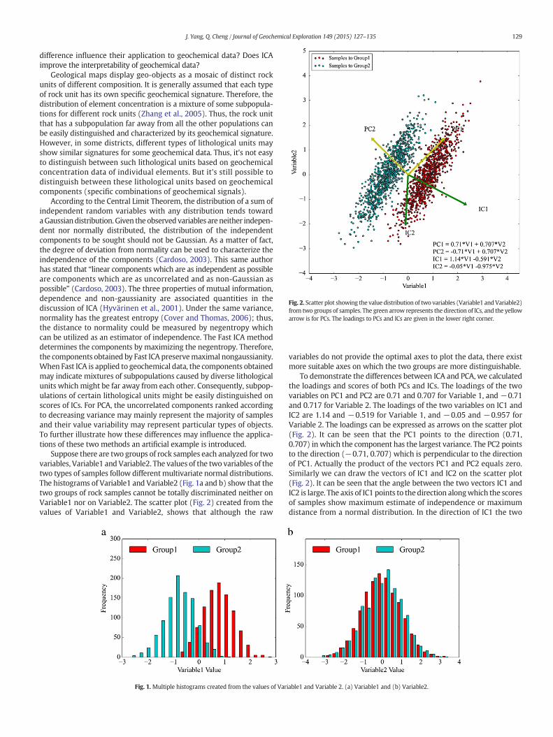
Fig. 2. Scatter plot showing the value distribution of two variables (Variable1 andVariable2)from two groups of samples. The green arrow represents the direction of ICs, and the yellowarrow is for PCs. The loadings to PCs and ICs are given in the lower right corner.

129J. Yang, Q. Cheng / Journal of Geochemical Exploration 149 (2015) 127–135

difference influence their application to geochemical data? Does ICAimprove the interpretability of geochemical data?

Geological maps display geo-objects as a mosaic of distinct rockunits of different composition. It is generally assumed that each typeof rock unit has its own specific geochemical signature. Therefore, thedistribution of element concentration is a mixture of some subpopula-tions for different rock units (Zhang et al., 2005). Thus, the rock unitthat has a subpopulation far away from all the other populations canbe easily distinguished and characterized by its geochemical signature.However, in some districts, different types of lithological units mayshow similar signatures for some geochemical data. Thus, it's not easyto distinguish between such lithological units based on geochemicalconcentration data of individual elements. But it's still possible todistinguish between these lithological units based on geochemicalcomponents (specific combinations of geochemical signals).

According to the Central Limit Theorem, the distribution of a sum ofindependent random variables with any distribution tends towardaGaussiandistribution. Given the observed variables are neither indepen-dent nor normally distributed, the distribution of the independentcomponents to be sought should not be Gaussian. As a matter of fact,the degree of deviation from normality can be used to characterize theindependence of the components (Cardoso, 2003). This same authorhas stated that “linear components which are as independent as possibleare components which are as uncorrelated and as non-Gaussian aspossible” (Cardoso, 2003). The three properties of mutual information,dependence and non-gaussianity are associated quantities in thediscussion of ICA (Hyvärinen et al., 2001). Under the same variance,normality has the greatest entropy (Cover and Thomas, 2006); thus,the distance to normality could be measured by negentropy whichcan be utilized as an estimator of independence. The Fast ICA methoddetermines the components by maximizing the negentropy. Therefore,the components obtained by Fast ICA preservemaximal nongaussianity.When Fast ICA is applied to geochemical data, the components obtainedmay indicate mixtures of subpopulations caused by diverse lithologicalunits which might be far away from each other. Consequently, subpop-ulations of certain lithological units might be easily distinguished onscores of ICs. For PCA, the uncorrelated components ranked accordingto decreasing variance may mainly represent the majority of samplesand their value variability may represent particular types of objects.To further illustrate how these differences may influence the applica-tions of these two methods an artificial example is introduced.

Suppose there are two groups of rock samples each analyzed for twovariables, Variable1 and Variable2. The values of the two variables of thetwo types of samples follow differentmultivariate normal distributions.The histograms of Variable1 and Variable2 (Fig. 1a and b) show that thetwo groups of rock samples cannot be totally discriminated neither onVariable1 nor on Variable2. The scatter plot (Fig. 2) created from thevalues of Variable1 and Variable2, shows that although the raw

Fig. 1. Multiple histograms created from the values of Var

variables do not provide the optimal axes to plot the data, there existmore suitable axes on which the two groups are more distinguishable.

To demonstrate the differences between ICA and PCA, we calculatedthe loadings and scores of both PCs and ICs. The loadings of the twovariables on PC1 and PC2 are 0.71 and 0.707 for Variable 1, and −0.71and 0.717 for Variable 2. The loadings of the two variables on IC1 andIC2 are 1.14 and −0.519 for Variable 1, and −0.05 and −0.957 forVariable 2. The loadings can be expressed as arrows on the scatter plot(Fig. 2). It can be seen that the PC1 points to the direction (0.71,0.707) in which the component has the largest variance. The PC2 pointsto the direction (−0.71, 0.707) which is perpendicular to the directionof PC1. Actually the product of the vectors PC1 and PC2 equals zero.Similarly we can draw the vectors of IC1 and IC2 on the scatter plot(Fig. 2). It can be seen that the angle between the two vectors IC1 andIC2 is large. The axis of IC1 points to the direction alongwhich the scoresof samples show maximum estimate of independence or maximumdistance from a normal distribution. In the direction of IC1 the two

iable1 and Variable 2. (a) Variable1 and (b) Variable2.

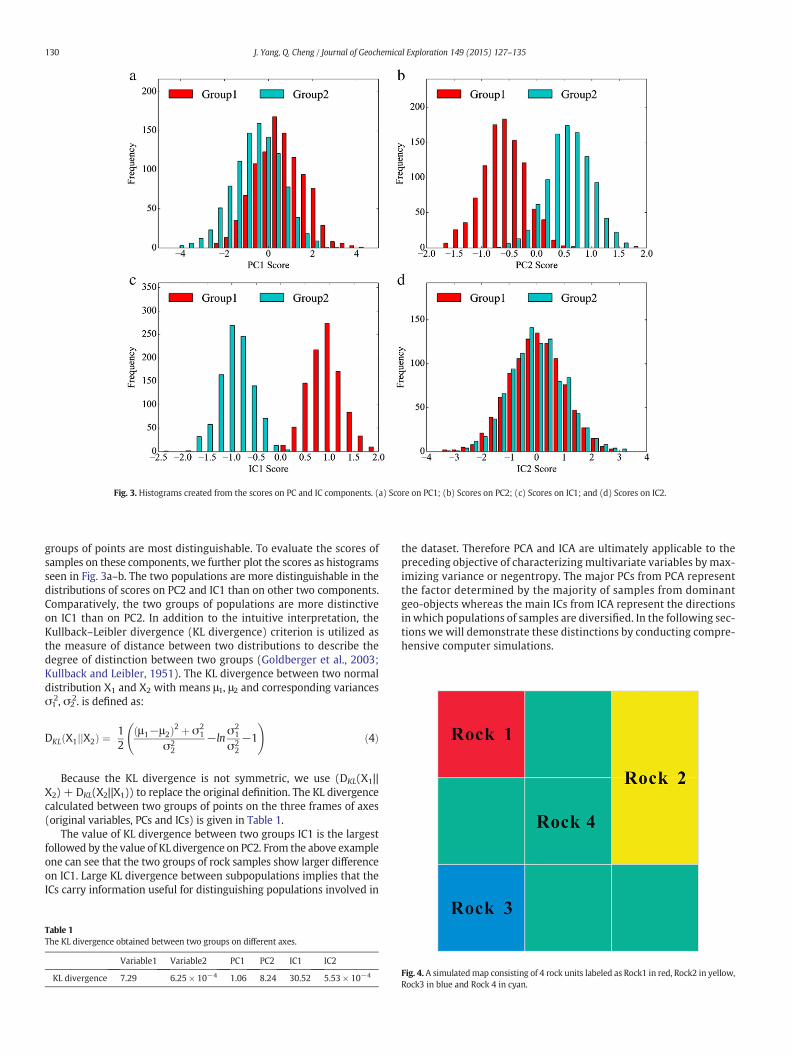
Fig. 3. Histograms created from the scores on PC and IC components. (a) Score on PC1; (b) Scores on PC2; (c) Scores on IC1; and (d) Scores on IC2.

130 J. Yang, Q. Cheng / Journal of Geochemical Exploration 149 (2015) 127–135

groups of points are most distinguishable. To evaluate the scores ofsamples on these components, we further plot the scores as histogramsseen in Fig. 3a–b. The two populations are more distinguishable in thedistributions of scores on PC2 and IC1 than on other two components.Comparatively, the two groups of populations are more distinctiveon IC1 than on PC2. In addition to the intuitive interpretation, theKullback–Leibler divergence (KL divergence) criterion is utilized asthe measure of distance between two distributions to describe thedegree of distinction between two groups (Goldberger et al., 2003;Kullback and Leibler, 1951). The KL divergence between two normaldistribution X1 and X2 with means μ1, μ2 and corresponding variancesσ1

2, σ22. is defined as:

DKL X1jjX2ð Þ ¼ 12

μ1−μ2ð Þ2 þ σ21

σ22

−lnσ2

1

σ22

−1

!ð4Þ

Because the KL divergence is not symmetric, we use (DKL(X1||X2) + DKL(X2||X1)) to replace the original definition. The KL divergencecalculated between two groups of points on the three frames of axes(original variables, PCs and ICs) is given in Table 1.

The value of KL divergence between two groups IC1 is the largestfollowed by the value of KL divergence on PC2. From the above exampleone can see that the two groups of rock samples show larger differenceon IC1. Large KL divergence between subpopulations implies that theICs carry information useful for distinguishing populations involved in

Table 1The KL divergence obtained between two groups on different axes.

Variable1 Variable2 PC1 PC2 IC1 IC2

KL divergence 7.29 6.25 × 10−4 1.06 8.24 30.52 5.53 × 10−4

the dataset. Therefore PCA and ICA are ultimately applicable to thepreceding objective of characterizing multivariate variables by max-imizing variance or negentropy. The major PCs from PCA representthe factor determined by the majority of samples from dominantgeo-objects whereas the main ICs from ICA represent the directionsin which populations of samples are diversified. In the following sec-tions we will demonstrate these distinctions by conducting compre-hensive computer simulations.

Fig. 4.A simulatedmap consisting of 4 rock units labeled as Rock1 in red, Rock2 in yellow,Rock3 in blue and Rock 4 in cyan.

131J. Yang, Q. Cheng / Journal of Geochemical Exploration 149 (2015) 127–135

3. Comparison of PCA and ICA by computer simulations

3.1. A simple computer simulation

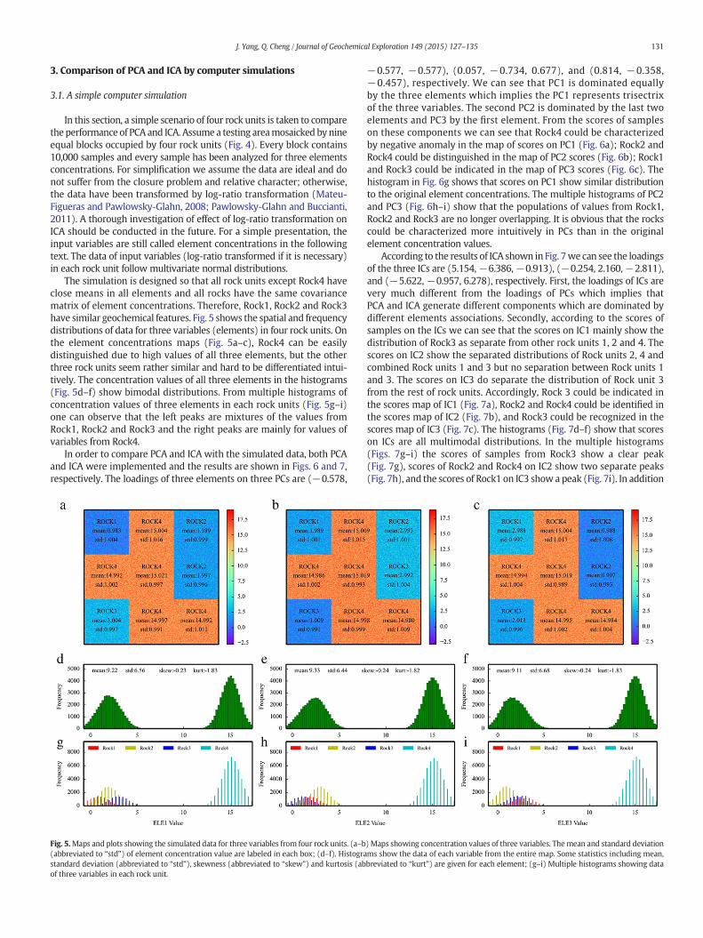
In this section, a simple scenario of four rock units is taken to comparethe performance of PCA and ICA. Assume a testing areamosaicked bynineequal blocks occupied by four rock units (Fig. 4). Every block contains10,000 samples and every sample has been analyzed for three elementsconcentrations. For simplification we assume the data are ideal and donot suffer from the closure problem and relative character; otherwise,the data have been transformed by log-ratio transformation (Mateu-Figueras and Pawlowsky-Glahn, 2008; Pawlowsky-Glahn and Buccianti,2011). A thorough investigation of effect of log-ratio transformation onICA should be conducted in the future. For a simple presentation, theinput variables are still called element concentrations in the followingtext. The data of input variables (log-ratio transformed if it is necessary)in each rock unit follow multivariate normal distributions.

The simulation is designed so that all rock units except Rock4 haveclose means in all elements and all rocks have the same covariancematrix of element concentrations. Therefore, Rock1, Rock2 and Rock3have similar geochemical features. Fig. 5 shows the spatial and frequencydistributions of data for three variables (elements) in four rock units. Onthe element concentrations maps (Fig. 5a–c), Rock4 can be easilydistinguished due to high values of all three elements, but the otherthree rock units seem rather similar and hard to be differentiated intui-tively. The concentration values of all three elements in the histograms(Fig. 5d–f) show bimodal distributions. From multiple histograms ofconcentration values of three elements in each rock units (Fig. 5g–i)one can observe that the left peaks are mixtures of the values fromRock1, Rock2 and Rock3 and the right peaks are mainly for values ofvariables from Rock4.

In order to compare PCA and ICA with the simulated data, both PCAand ICA were implemented and the results are shown in Figs. 6 and 7,respectively. The loadings of three elements on three PCs are (−0.578,

Fig. 5.Maps and plots showing the simulated data for three variables from four rock units. (a–b(abbreviated to “std”) of element concentration value are labeled in each box; (d–f). Histograstandard deviation (abbreviated to “std”), skewness (abbreviated to “skew”) and kurtosis (abof three variables in each rock unit.

−0.577, −0.577), (0.057, −0.734, 0.677), and (0.814, −0.358,−0.457), respectively. We can see that PC1 is dominated equallyby the three elements which implies the PC1 represents trisectrixof the three variables. The second PC2 is dominated by the last twoelements and PC3 by the first element. From the scores of sampleson these components we can see that Rock4 could be characterizedby negative anomaly in the map of scores on PC1 (Fig. 6a); Rock2 andRock4 could be distinguished in the map of PC2 scores (Fig. 6b); Rock1and Rock3 could be indicated in the map of PC3 scores (Fig. 6c). Thehistogram in Fig. 6g shows that scores on PC1 show similar distributionto the original element concentrations. The multiple histograms of PC2and PC3 (Fig. 6h–i) show that the populations of values from Rock1,Rock2 and Rock3 are no longer overlapping. It is obvious that the rockscould be characterized more intuitively in PCs than in the originalelement concentration values.

According to the results of ICA shown in Fig. 7we can see the loadingsof the three ICs are (5.154,−6.386,−0.913), (−0.254, 2.160,−2.811),and (−5.622, −0.957, 6.278), respectively. First, the loadings of ICs arevery much different from the loadings of PCs which implies thatPCA and ICA generate different components which are dominated bydifferent elements associations. Secondly, according to the scores ofsamples on the ICs we can see that the scores on IC1 mainly show thedistribution of Rock3 as separate from other rock units 1, 2 and 4. Thescores on IC2 show the separated distributions of Rock units 2, 4 andcombined Rock units 1 and 3 but no separation between Rock units 1and 3. The scores on IC3 do separate the distribution of Rock unit 3from the rest of rock units. Accordingly, Rock 3 could be indicated inthe scores map of IC1 (Fig. 7a), Rock2 and Rock4 could be identified inthe scores map of IC2 (Fig. 7b), and Rock3 could be recognized in thescores map of IC3 (Fig. 7c). The histograms (Fig. 7d–f) show that scoreson ICs are all multimodal distributions. In the multiple histograms(Figs. 7g–i) the scores of samples from Rock3 show a clear peak(Fig. 7g), scores of Rock2 and Rock4 on IC2 show two separate peaks(Fig. 7h), and the scores of Rock1 on IC3 show a peak (Fig. 7i). In addition

) Maps showing concentration values of three variables. Themean and standard deviationms show the data of each variable from the entire map. Some statistics including mean,breviated to “kurt”) are given for each element; (g–i) Multiple histograms showing data

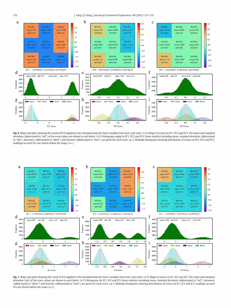
Fig. 6.Maps and plots showing the result of PCA applied to the simulated data for three variables from four rock units. (a–b)Maps of scores on PC1, PC2 and PC3. Themean and standarddeviation (abbreviated to “std”) of the score values are shown in each block. (d–f) Histograms apply to PC1, PC2 and PC3. Some statistics includingmean, standard deviation (abbreviatedto “std”), skewness (abbreviated to “skew”) and kurtosis (abbreviated to “kurt”) are given for each score. (g–i) Multiple histograms showing distribution of scores on PC1, PC2 and PC3.Loadings on each PCs are shown below the maps (a–c).

Fig. 7.Maps and plots showing the result of ICA applied to the simulated data for three variables from four rock units. (a–b) Maps of scores on IC1, IC2 and IC3. The mean and standarddeviation (std) of the score values are shown in each block. (d–f) Histograms for IC1, IC2 and IC3. Some statistics including mean, standard deviation (abbreviated to “std”), skewness(abbreviated to “skew”) and kurtosis (abbreviated to “kurt”) are given for each score. (g–i) Multiple histograms showing distribution of scores on IC1, IC2 and IC3. Loadings on eachPCs are shown below the maps (a–c).

132 J. Yang, Q. Cheng / Journal of Geochemical Exploration 149 (2015) 127–135

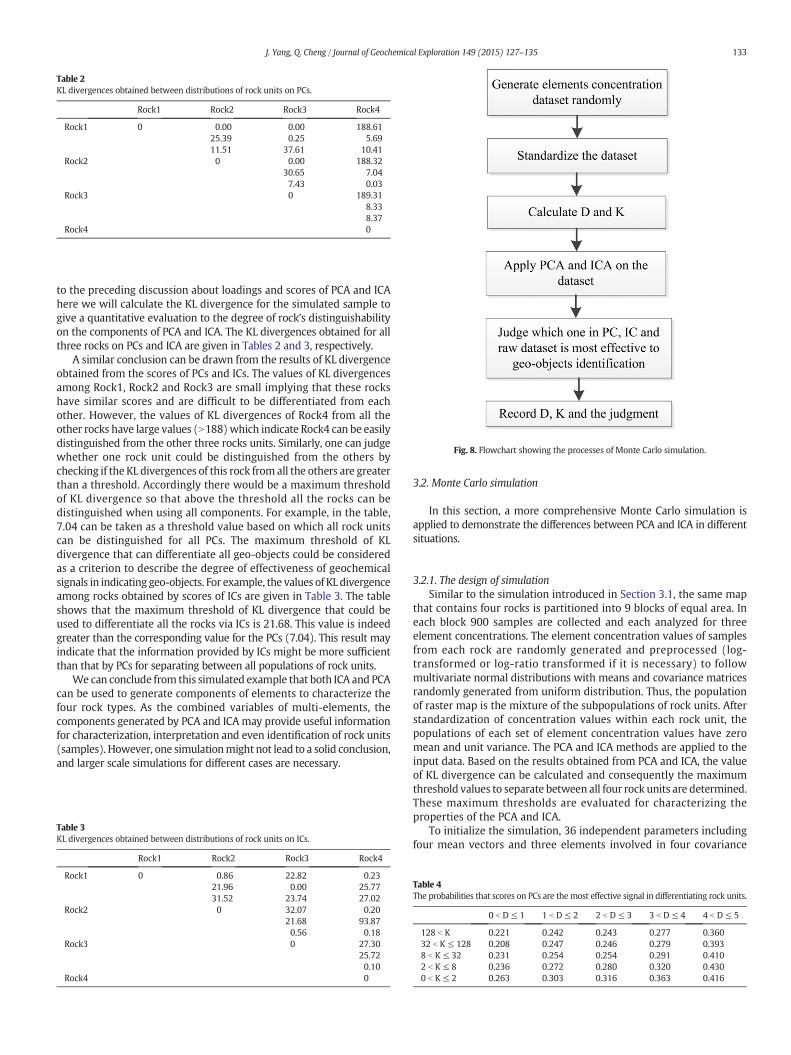
Fig. 8. Flowchart showing the processes of Monte Carlo simulation.

Table 2KL divergences obtained between distributions of rock units on PCs.

Rock1 Rock2 Rock3 Rock4

Rock1 0 0.00 0.00 188.6125.39 0.25 5.6911.51 37.61 10.41

Rock2 0 0.00 188.3230.65 7.047.43 0.03

Rock3 0 189.318.338.37

Rock4 0

133J. Yang, Q. Cheng / Journal of Geochemical Exploration 149 (2015) 127–135

to the preceding discussion about loadings and scores of PCA and ICAhere we will calculate the KL divergence for the simulated sample togive a quantitative evaluation to the degree of rock's distinguishabilityon the components of PCA and ICA. The KL divergences obtained for allthree rocks on PCs and ICA are given in Tables 2 and 3, respectively.

A similar conclusion can be drawn from the results of KL divergenceobtained from the scores of PCs and ICs. The values of KL divergencesamong Rock1, Rock2 and Rock3 are small implying that these rockshave similar scores and are difficult to be differentiated from eachother. However, the values of KL divergences of Rock4 from all theother rocks have large values (N188)which indicate Rock4 can be easilydistinguished from the other three rocks units. Similarly, one can judgewhether one rock unit could be distinguished from the others bychecking if the KL divergences of this rock from all the others are greaterthan a threshold. Accordingly there would be a maximum thresholdof KL divergence so that above the threshold all the rocks can bedistinguished when using all components. For example, in the table,7.04 can be taken as a threshold value based on which all rock unitscan be distinguished for all PCs. The maximum threshold of KLdivergence that can differentiate all geo-objects could be consideredas a criterion to describe the degree of effectiveness of geochemicalsignals in indicating geo-objects. For example, the values of KL divergenceamong rocks obtained by scores of ICs are given in Table 3. The tableshows that the maximum threshold of KL divergence that could beused to differentiate all the rocks via ICs is 21.68. This value is indeedgreater than the corresponding value for the PCs (7.04). This result mayindicate that the information provided by ICs might be more sufficientthan that by PCs for separating between all populations of rock units.

We can conclude from this simulated example that both ICA and PCAcan be used to generate components of elements to characterize thefour rock types. As the combined variables of multi-elements, thecomponents generated by PCA and ICAmay provide useful informationfor characterization, interpretation and even identification of rock units(samples). However, one simulationmight not lead to a solid conclusion,and larger scale simulations for different cases are necessary.

Table 3KL divergences obtained between distributions of rock units on ICs.

Rock1 Rock2 Rock3 Rock4

Rock1 0 0.86 22.82 0.2321.96 0.00 25.7731.52 23.74 27.02

Rock2 0 32.07 0.2021.68 93.870.56 0.18

Rock3 0 27.3025.720.10

Rock4 0

3.2. Monte Carlo simulation

In this section, a more comprehensive Monte Carlo simulation isapplied to demonstrate the differences between PCA and ICA in differentsituations.

3.2.1. The design of simulationSimilar to the simulation introduced in Section 3.1, the same map

that contains four rocks is partitioned into 9 blocks of equal area. Ineach block 900 samples are collected and each analyzed for threeelement concentrations. The element concentration values of samplesfrom each rock are randomly generated and preprocessed (log-transformed or log-ratio transformed if it is necessary) to followmultivariate normal distributions with means and covariance matricesrandomly generated from uniform distribution. Thus, the populationof raster map is the mixture of the subpopulations of rock units. Afterstandardization of concentration values within each rock unit, thepopulations of each set of element concentration values have zeromean and unit variance. The PCA and ICA methods are applied to theinput data. Based on the results obtained from PCA and ICA, the valueof KL divergence can be calculated and consequently the maximumthreshold values to separate between all four rock units are determined.These maximum thresholds are evaluated for characterizing theproperties of the PCA and ICA.

To initialize the simulation, 36 independent parameters includingfour mean vectors and three elements involved in four covariance

Table 4The probabilities that scores on PCs are themost effective signal in differentiating rock units.

0 b D ≤ 1 1 b D ≤ 2 2 b D ≤ 3 3 b D ≤ 4 4 b D ≤ 5

128 b K 0.221 0.242 0.243 0.277 0.36032 b K ≤ 128 0.208 0.247 0.246 0.279 0.3938 b K ≤ 32 0.231 0.254 0.254 0.291 0.4102 b K ≤ 8 0.236 0.272 0.280 0.320 0.4300 b K ≤ 2 0.263 0.303 0.316 0.363 0.416

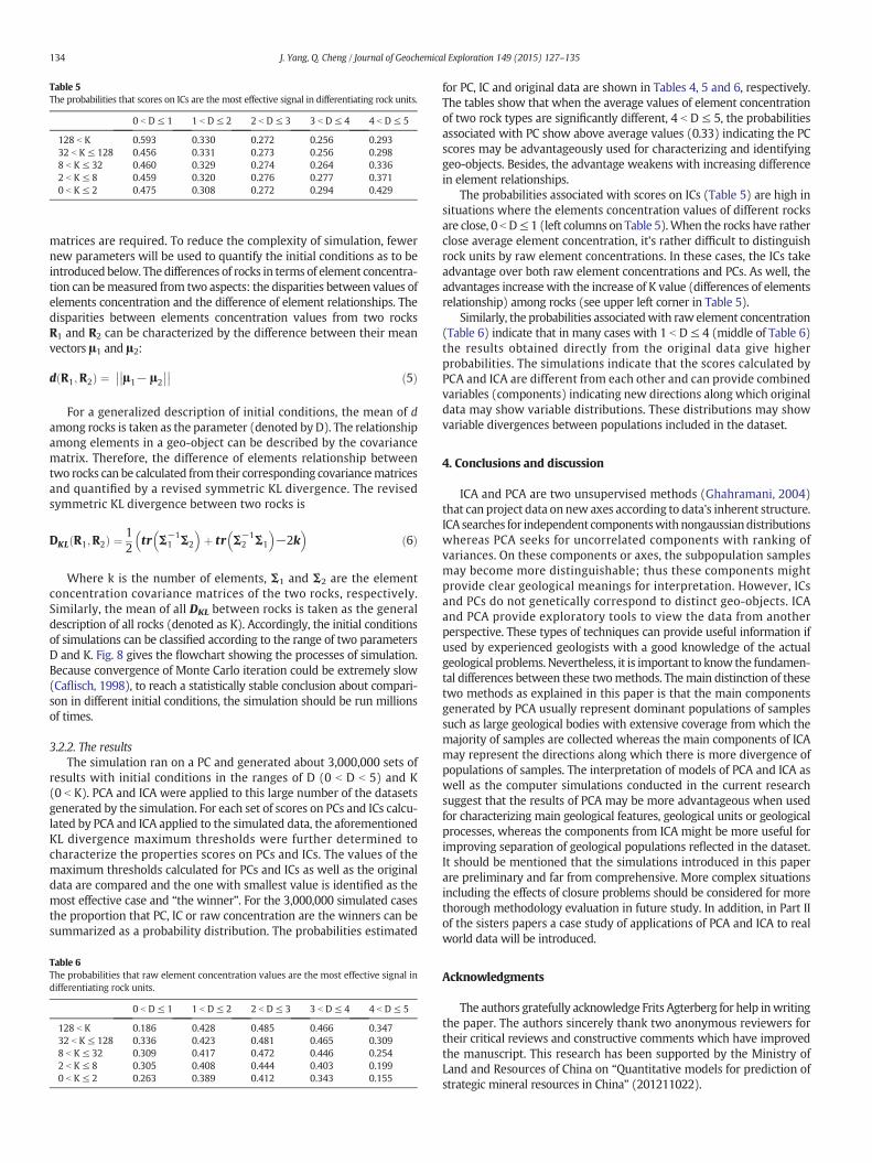
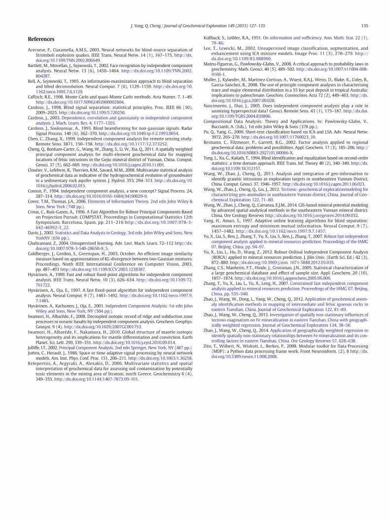
Table 5The probabilities that scores on ICs are the most effective signal in differentiating rock units.

0 b D ≤ 1 1 b D ≤ 2 2 b D ≤ 3 3 b D ≤ 4 4 b D ≤ 5

128 b K 0.593 0.330 0.272 0.256 0.29332 b K ≤ 128 0.456 0.331 0.273 0.256 0.2988 b K ≤ 32 0.460 0.329 0.274 0.264 0.3362 b K ≤ 8 0.459 0.320 0.276 0.277 0.3710 b K ≤ 2 0.475 0.308 0.272 0.294 0.429

134 J. Yang, Q. Cheng / Journal of Geochemical Exploration 149 (2015) 127–135

matrices are required. To reduce the complexity of simulation, fewernew parameters will be used to quantify the initial conditions as to beintroduced below. The differences of rocks in terms of element concentra-tion can bemeasured from two aspects: the disparities between values ofelements concentration and the difference of element relationships. Thedisparities between elements concentration values from two rocksR1 and R2 can be characterized by the difference between their meanvectors μ1 and μ2:

d R1;R2ð Þ ¼ μ1− μ2

�� ���� �� ð5Þ

For a generalized description of initial conditions, the mean of damong rocks is taken as the parameter (denoted by D). The relationshipamong elements in a geo-object can be described by the covariancematrix. Therefore, the difference of elements relationship betweentwo rocks can be calculated from their corresponding covariancematricesand quantified by a revised symmetric KL divergence. The revisedsymmetric KL divergence between two rocks is

DKL R1;R2ð Þ ¼ 12

tr Σ−11 Σ2

� �þ tr Σ−1

2 Σ1

� �−2k

� �ð6Þ

Where k is the number of elements, Σ1 and Σ2 are the elementconcentration covariance matrices of the two rocks, respectively.Similarly, the mean of all DKL between rocks is taken as the generaldescription of all rocks (denoted as K). Accordingly, the initial conditionsof simulations can be classified according to the range of two parametersD and K. Fig. 8 gives the flowchart showing the processes of simulation.Because convergence of Monte Carlo iteration could be extremely slow(Caflisch, 1998), to reach a statistically stable conclusion about compari-son in different initial conditions, the simulation should be run millionsof times.

3.2.2. The resultsThe simulation ran on a PC and generated about 3,000,000 sets of

results with initial conditions in the ranges of D (0 b D b 5) and K(0 b K). PCA and ICA were applied to this large number of the datasetsgenerated by the simulation. For each set of scores on PCs and ICs calcu-lated by PCA and ICA applied to the simulated data, the aforementionedKL divergence maximum thresholds were further determined tocharacterize the properties scores on PCs and ICs. The values of themaximum thresholds calculated for PCs and ICs as well as the originaldata are compared and the one with smallest value is identified as themost effective case and “the winner”. For the 3,000,000 simulated casesthe proportion that PC, IC or raw concentration are the winners can besummarized as a probability distribution. The probabilities estimated

Table 6The probabilities that raw element concentration values are the most effective signal indifferentiating rock units.

0 b D ≤ 1 1 b D ≤ 2 2 b D ≤ 3 3 b D ≤ 4 4 b D ≤ 5

128 b K 0.186 0.428 0.485 0.466 0.34732 b K ≤ 128 0.336 0.423 0.481 0.465 0.3098 b K ≤ 32 0.309 0.417 0.472 0.446 0.2542 b K ≤ 8 0.305 0.408 0.444 0.403 0.1990 b K ≤ 2 0.263 0.389 0.412 0.343 0.155

for PC, IC and original data are shown in Tables 4, 5 and 6, respectively.The tables show that when the average values of element concentrationof two rock types are significantly different, 4 b D ≤ 5, the probabilitiesassociated with PC show above average values (0.33) indicating the PCscores may be advantageously used for characterizing and identifyinggeo-objects. Besides, the advantage weakens with increasing differencein element relationships.

The probabilities associated with scores on ICs (Table 5) are high insituations where the elements concentration values of different rocksare close, 0 b D≤ 1 (left columns on Table 5).When the rocks have ratherclose average element concentration, it's rather difficult to distinguishrock units by raw element concentrations. In these cases, the ICs takeadvantage over both raw element concentrations and PCs. As well, theadvantages increase with the increase of K value (differences of elementsrelationship) among rocks (see upper left corner in Table 5).

Similarly, the probabilities associatedwith raw element concentration(Table 6) indicate that in many cases with 1 b D ≤ 4 (middle of Table 6)the results obtained directly from the original data give higherprobabilities. The simulations indicate that the scores calculated byPCA and ICA are different from each other and can provide combinedvariables (components) indicating new directions along which originaldata may show variable distributions. These distributions may showvariable divergences between populations included in the dataset.

4. Conclusions and discussion

ICA and PCA are two unsupervised methods (Ghahramani, 2004)that can project data on new axes according to data's inherent structure.ICA searches for independent componentswithnongaussiandistributionswhereas PCA seeks for uncorrelated components with ranking ofvariances. On these components or axes, the subpopulation samplesmay become more distinguishable; thus these components mightprovide clear geological meanings for interpretation. However, ICsand PCs do not genetically correspond to distinct geo-objects. ICAand PCA provide exploratory tools to view the data from anotherperspective. These types of techniques can provide useful information ifused by experienced geologists with a good knowledge of the actualgeological problems. Nevertheless, it is important to know the fundamen-tal differences between these twomethods. Themain distinction of thesetwo methods as explained in this paper is that the main componentsgenerated by PCA usually represent dominant populations of samplessuch as large geological bodies with extensive coverage from which themajority of samples are collected whereas the main components of ICAmay represent the directions along which there is more divergence ofpopulations of samples. The interpretation of models of PCA and ICA aswell as the computer simulations conducted in the current researchsuggest that the results of PCA may be more advantageous when usedfor characterizing main geological features, geological units or geologicalprocesses, whereas the components from ICA might be more useful forimproving separation of geological populations reflected in the dataset.It should be mentioned that the simulations introduced in this paperare preliminary and far from comprehensive. More complex situationsincluding the effects of closure problems should be considered for morethorough methodology evaluation in future study. In addition, in Part IIof the sisters papers a case study of applications of PCA and ICA to realworld data will be introduced.

Acknowledgments

The authors gratefully acknowledge Frits Agterberg for help inwritingthe paper. The authors sincerely thank two anonymous reviewers fortheir critical reviews and constructive comments which have improvedthe manuscript. This research has been supported by the Ministry ofLand and Resources of China on “Quantitative models for prediction ofstrategic mineral resources in China” (201211022).

135J. Yang, Q. Cheng / Journal of Geochemical Exploration 149 (2015) 127–135

References

Acernese, F., Ciaramella, A.M.S., 2003. Neural networks for blind-source separation ofStromboli explosion quakes. IEEE Trans. Neural Netw. 14 (1), 167–175. http://dx.doi.org/10.1109/TNN.2002.806649.

Bartlett, M., Movellan, J., Sejnowski, T., 2002. Face recognition by independent componentanalysis. Neural Netw. 13 (6), 1450–1464. http://dx.doi.org/10.1109/TNN.2002.804287.

Bell, A., Sejnowski, T., 1995. An information-maximization approach to blind separationand blind deconvolution. Neural Comput. 7 (6), 1129–1159. http://dx.doi.org/10.1162/neco.1995.7.6.1129.

Caflisch, R.E., 1998. Monte Carlo and quasi-Monte Carlo methods. Acta Numer. 7, 1–49.http://dx.doi.org/10.1017/S0962492900002804.

Cardoso, J., 1998. Blind signal separation: statistical principles. Proc. IEEE 86 (10),2009–2025. http://dx.doi.org/10.1109/5.720250.

Cardoso, J., 2003. Dependence, correlation and gaussianity in independent componentanalysis. J. Mach. Learn. Res. 4, 1177–1203.

Cardoso, J., Souloumiac, A., 1993. Blind beamforming for non-gaussian signals. RadarSignal Process. 140 (6), 362–370. http://dx.doi.org/10.1049/ip-f-2.1993.0054.

Chen, C., Zhang, X., 1999. Independent component analysis for remote sensing study.Remote Sens. 3871, 150–158. http://dx.doi.org/10.1117/12.373252.

Cheng, Q., Bonham-Carter, G., Wang,W., Zhang, S., Li, W., Xia, Q., 2011. A spatially weightedprincipal component analysis for multi-element geochemical data for mappinglocations of felsic intrusions in the Gejiu mineral district of Yunnan, China. Comput.Geosci. 37 (5), 662–669. http://dx.doi.org/10.1016/j.cageo.2010.11.001.

Cloutier, V., Lefebvre, R., Therrien, R.M., Savard, M.M., 2008. Multivariate statistical analysisof geochemical data as indicative of the hydrogeochemical evolution of groundwaterin a sedimentary rock aquifer system. J. Hydrol. 353, 294–313. http://dx.doi.org/10.1016/j.jhydrol.2008.02.015.

Comon, P., 1994. Independent component analysis, a new concept? Signal Process. 24,287–314. http://dx.doi.org/10.1016/0165-1684(94)90029-9.

Cover, T.M., Thomas, J.A., 2006. Elements of Information Theory. 2nd edn John Wiley &Sons, New York (748 pp.).

Croux, C., Ruiz-Gazen, A., 1996. A Fast Algorithm for Robust Principal Components Basedon Projection Pursuit. COMPSTAT, Proceedings in Computational Statistics 12thSymposium, Barcelona, Spain, pp. 211–216 http://dx.doi.org/10.1007/978-3-642-46992-3_22.

Davis, J., 2002. Sratistics and Data Analysis in Geology. 3rd edn. JohnWiley and Sons, NewYorkNY (656 pp.).

Ghahramani, Z., 2004. Unsupervised learning. Adv. Lect. Mach. Learn. 72–112 http://dx.doi.org/10.1007/978-3-540-28650-9_5.

Goldberger, J., Gordon, S., Greenspan, H., 2003, October. An efficient image similaritymeasure based on approximations of KL-divergence between two Gaussianmixtures.Proceedings. Ninth IEEE International Conference on Computer Vision, 2003,pp. 487–493 http://dx.doi.org/10.1109/ICCV.2003.1238387.

Hyvärinen, A., 1999. Fast and robust fixed-point algorithms for independent componentanalysis. IEEE Trans. Neural Netw. 10 (3), 626–634. http://dx.doi.org/10.1109/72.761722.

Hyvärinen, A., Oja, E., 1997. A fast fixed-point algorithm for independent componentanalysis. Neural Comput. 9 (7), 1483–1492. http://dx.doi.org/10.1162/neco.1997.9.7.1483.

Hyvärinen, A., Karhunen, J., Oja, E., 2001. Indpendent Component Analysis. 1st edn JohnWiley and Sons, New York, NY (504 pp.).

Iwamori, H., Albarède, F., 2008. Decoupled isotopic record of ridge and subduction zoneprocesses in oceanic basalts by independent component analysis. Geochem. Geophys.Geosyst. 9 (4). http://dx.doi.org/10.1029/2007GC001753.

Iwamori, H., Albaréde, F., Nakamura, H., 2010. Global structure of mantle isotopicheterogeneity and its implications for mantle differentiation and convection. EarthPlanet. Sci. Lett. 299, 339–351. http://dx.doi.org/10.1016/j.epsl.2010.09.014.

Jolliffe, I.T., 2002. Principal Component Analysis. 2nd edn Springer, New York, NY (487 pp.).Jutten, C., Herault, J., 1986. Space or time adaptive signal processing by neural network

models. Am. Inst. Phys. Conf. Proc. 151, 206–211. http://dx.doi.org/10.1063/1.36258.Kelepertsis, A., Argyraki, A., Alexakis, D., 2006. Multivariate statistics and spatial

interpretation of geochemical data for assessing soil contamination by potentiallytoxic elements in the mining area of Stratoni, north Greece. Geochemistry 6 (4),349–355. http://dx.doi.org/10.1144/1467-7873/05-101.

Kullback, S., Leibler, R.A., 1951. On information and sufficiency. Ann. Math. Stat. 22 (1),79–86.

Lee, T., Lewicki, M., 2002. Unsupervised image classification, segmentation, andenhancement using ICA mixture models. Image Proc. 11 (3), 270–279. http://dx.doi.org/10.1109/83.988960.

Mateu-Figueras, G., Pawlowsky-Glahn, V., 2008. A critical approach to probability laws ingeochemistry. Math. Geosci. 40 (5), 489–502. http://dx.doi.org/10.1007/s11004-008-9169-1.

Muller, J., Kylander, M., Martinez-Cortizas, A., Wuest, R.A.J., Weiss, D., Blake, K., Coles, B.,Garcia-Sanchez, R., 2008. The use of principle component analyses in characterisingtrace and major elemental distribution in a 55 kyr peat deposit in tropical Australia:implications to paleoclimate. Geochim. Cosmochim. Acta 72 (2), 449–463. http://dx.doi.org/10.1016/j.gca.2007.09.028.

Nascimento, J., Dias, J., 2005. Does independent component analysis play a role inunmixing hyperspectral data? Geosci. Remote Sens. 43 (1), 175–187. http://dx.doi.org/10.1109/TGRS.2004.839806.

Compositional Data Analysis: Theory and Applications. In: Pawlowsky-Glahn, V.,Buccianti, A. (Eds.), 1st edn John Wiley & Sons (378 pp.).

Pu, Q., Yang, G., 2006. Short-text classification based on ICA and LSA. Adv. Neural Netw.3972, 265–270. http://dx.doi.org/10.1007/11760023_39.

Reimann, C., Filzmoser, P., Garrett, R.G., 2002. Factor analysis applied to regionalgeochemical data: problems and possibilities. Appl. Geochem. 17 (3), 185–206. http://dx.doi.org/10.1016/S0883-2927(01)00066-X.

Tong, L., Xu, G., Kailath, T., 1994. Blind identification and equalization based on second-orderstatistics: a time domain approach. IEEE Trans. Inf. Theory 40 (2), 340–349. http://dx.doi.org/10.1109/18.312157.

Wang, W., Zhao, J., Cheng, Q., 2011. Analysis and integration of geo-information toidentify granitic intrusions as exploration targets in southeastern Yunnan District,China. Comput. Geosci. 37, 1946–1957. http://dx.doi.org/10.1016/j.cageo.2011.06.023.

Wang, W., Zhao, J., Cheng, Q., Liu, J., 2012. Tectonic–geochemical explorationmodeling forcharacterizing geo-anomalies in southeastern Yunnan district, China. Journal of Geo-chemical Exploration 122, 71–80.

Wang,W., Zhao, J., Cheng, Q., Carranza, E.J.M., 2014. GIS-basedmineral potential modelingby advanced spatial analytical methods in the southeastern Yunnan mineral district.China, Ore Geology Reviews http://dx.doi.org/10.1016/j.oregeorev.2014.09.032.

Yang, H., Amari, S., 1997. Adaptive online learning algorithms for blind separation:maximum entropy and minimum mutual information. Neural Comput. 9 (7),1457–1482. http://dx.doi.org/10.1162/neco.1997.9.7.1457.

Yu, X., Liu, S., Ren, J., Zhang, T., Yu, X., Liu, S., Ren, J., Zhang, T., 2007. Robust fast independentcomponent analysis applied to mineral resources prediction. Proceedings of the IAMG07, Beijing, China, pp. 94–97.

Yu, X., Liu, L., Hu, D., Wang, Z., 2012. Robust Ordinal Independent Component Analysis(ROICA) applied to mineral resources prediction. J. Jilin Univ. (Earth Sci. Ed.) 42 (3),872–880. http://dx.doi.org/10.3969/j.issn. 1671-5888.2012.03.035.

Zhang, C.S., Manheim, F.T., Hinde, J., Grossman, J.N., 2005. Statistical characterization ofa large geochemical database and effect of sample size. Appl. Geochem. 20 (10),1857–1874. http://dx.doi.org/10.1016/j.apgeochem.2005.06.006.

Zhang, T., Yu, X., Liu, L., Yu, X., Leng, H., 2007. Constrained fast independent componentanalysis applied to mineral resources prediction. Proceedings of the IAMG 07, Beijing,China, pp. 535–540.

Zhao, J., Wang, W., Dong, L., Yang, W., Cheng, Q., 2012. Application of geochemical anom-aly identification methods in mapping of intermediate and felsic igneous rocks ineastern Tianshan, China. Journal of Geochemical Exploration 122, 81–89.

Zhao, J., Wang, W., Cheng, Q., 2013. Investigation of spatially non-stationary influences oftectono-magmatism on Fe mineralization in eastern Tianshan, China with geograph-ically weighted regression. Journal of Geochemical Exploration 134, 38–50.

Zhao, J., Wang, W., Cheng, Q., 2014. Application of geographically weighted regression toidentify spatially non-stationary relationships between Femineralization and its con-trolling factors in eastern Tianshan, China. Ore Geology Reviews 57, 628–638.

Zito, T., Wilbert, N., Wiskott, L., Berkes, P., 2008. Modular toolkit for Data Processing(MDP): a Python data processing frame work. Front Neuroinform. (2), 8 http://dx.doi.org/10.3389/neuro.11.008.2008.