Junction Tree Variational Autoencoder for Molecular Graph Generation

Wengong Jin 1 Regina Barzilay 1 Tommi Jaakkola 1

Abstract

We seek to automate the design of moleculesbased on specific chemical properties. In com-putational terms, this task involves continuousembedding and generation of molecular graphs.Our primary contribution is the direct realizationof molecular graphs, a task previously approachedby generating linear SMILES strings instead ofgraphs. Our junction tree variational autoencodergenerates molecular graphs in two phases, by firstgenerating a tree-structured scaffold over chemi-cal substructures, and then combining them into amolecule with a graph message passing network.This approach allows us to incrementally expandmolecules while maintaining chemical validityat every step. We evaluate our model on multi-ple tasks ranging from molecular generation tooptimization. Across these tasks, our model out-performs previous state-of-the-art baselines by asignificant margin.

1. IntroductionThe key challenge of drug discovery is to find targetmolecules with desired chemical properties. Currently, thistask takes years of development and exploration by expertchemists and pharmacologists. Our ultimate goal is to au-tomate this process. From a computational perspective, wedecompose the challenge into two complementary subtasks:learning to represent molecules in a continuous manner thatfacilitates the prediction and optimization of their properties(encoding); and learning to map an optimized continuousrepresentation back into a molecular graph with improvedproperties (decoding). While deep learning has been exten-sively investigated for molecular graph encoding (Duvenaudet al., 2015; Kearnes et al., 2016; Gilmer et al., 2017), theharder combinatorial task of molecular graph generationfrom latent representation remains under-explored.

1MIT Computer Science & Artificial Intelligence Lab. Corre-spondence to: Wengong Jin <wengong@csail.mit.edu>.

Proceedings of the 35 th International Conference on MachineLearning, Stockholm, Sweden, PMLR 80, 2018. Copyright 2018by the author(s).

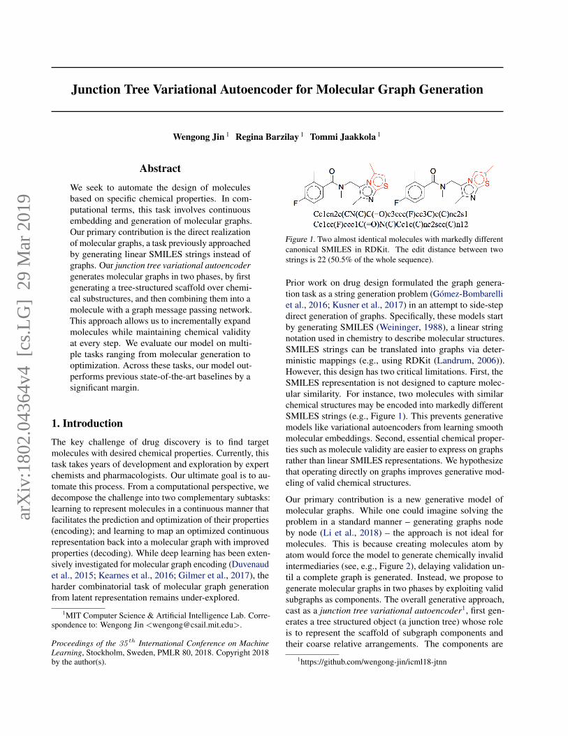
Figure 1. Two almost identical molecules with markedly differentcanonical SMILES in RDKit. The edit distance between twostrings is 22 (50.5% of the whole sequence).

Prior work on drug design formulated the graph genera-tion task as a string generation problem (Gomez-Bombarelliet al., 2016; Kusner et al., 2017) in an attempt to side-stepdirect generation of graphs. Specifically, these models startby generating SMILES (Weininger, 1988), a linear stringnotation used in chemistry to describe molecular structures.SMILES strings can be translated into graphs via deter-ministic mappings (e.g., using RDKit (Landrum, 2006)).However, this design has two critical limitations. First, theSMILES representation is not designed to capture molec-ular similarity. For instance, two molecules with similarchemical structures may be encoded into markedly differentSMILES strings (e.g., Figure 1). This prevents generativemodels like variational autoencoders from learning smoothmolecular embeddings. Second, essential chemical proper-ties such as molecule validity are easier to express on graphsrather than linear SMILES representations. We hypothesizethat operating directly on graphs improves generative mod-eling of valid chemical structures.

Our primary contribution is a new generative model ofmolecular graphs. While one could imagine solving theproblem in a standard manner – generating graphs nodeby node (Li et al., 2018) – the approach is not ideal formolecules. This is because creating molecules atom byatom would force the model to generate chemically invalidintermediaries (see, e.g., Figure 2), delaying validation un-til a complete graph is generated. Instead, we propose togenerate molecular graphs in two phases by exploiting validsubgraphs as components. The overall generative approach,cast as a junction tree variational autoencoder1, first gen-erates a tree structured object (a junction tree) whose roleis to represent the scaffold of subgraph components andtheir coarse relative arrangements. The components are

1https://github.com/wengong-jin/icml18-jtnn

arX

iv:1

802.

0436

4v4

[cs

.LG

] 2

9 M

ar 2

019

Junction Tree Variational Autoencoder for Molecular Graph Generation

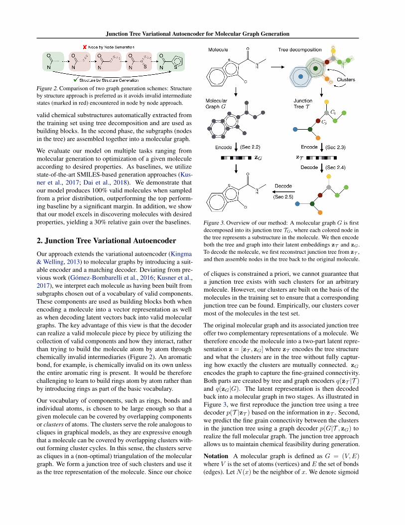
Figure 2. Comparison of two graph generation schemes: Structureby structure approach is preferred as it avoids invalid intermediatestates (marked in red) encountered in node by node approach.

valid chemical substructures automatically extracted fromthe training set using tree decomposition and are used asbuilding blocks. In the second phase, the subgraphs (nodesin the tree) are assembled together into a molecular graph.

We evaluate our model on multiple tasks ranging frommolecular generation to optimization of a given moleculeaccording to desired properties. As baselines, we utilizestate-of-the-art SMILES-based generation approaches (Kus-ner et al., 2017; Dai et al., 2018). We demonstrate thatour model produces 100% valid molecules when sampledfrom a prior distribution, outperforming the top perform-ing baseline by a significant margin. In addition, we showthat our model excels in discovering molecules with desiredproperties, yielding a 30% relative gain over the baselines.

2. Junction Tree Variational AutoencoderOur approach extends the variational autoencoder (Kingma& Welling, 2013) to molecular graphs by introducing a suit-able encoder and a matching decoder. Deviating from pre-vious work (Gomez-Bombarelli et al., 2016; Kusner et al.,2017), we interpret each molecule as having been built fromsubgraphs chosen out of a vocabulary of valid components.These components are used as building blocks both whenencoding a molecule into a vector representation as wellas when decoding latent vectors back into valid moleculargraphs. The key advantage of this view is that the decodercan realize a valid molecule piece by piece by utilizing thecollection of valid components and how they interact, ratherthan trying to build the molecule atom by atom throughchemically invalid intermediaries (Figure 2). An aromaticbond, for example, is chemically invalid on its own unlessthe entire aromatic ring is present. It would be thereforechallenging to learn to build rings atom by atom rather thanby introducing rings as part of the basic vocabulary.

Our vocabulary of components, such as rings, bonds andindividual atoms, is chosen to be large enough so that agiven molecule can be covered by overlapping componentsor clusters of atoms. The clusters serve the role analogous tocliques in graphical models, as they are expressive enoughthat a molecule can be covered by overlapping clusters with-out forming cluster cycles. In this sense, the clusters serveas cliques in a (non-optimal) triangulation of the moleculargraph. We form a junction tree of such clusters and use itas the tree representation of the molecule. Since our choice

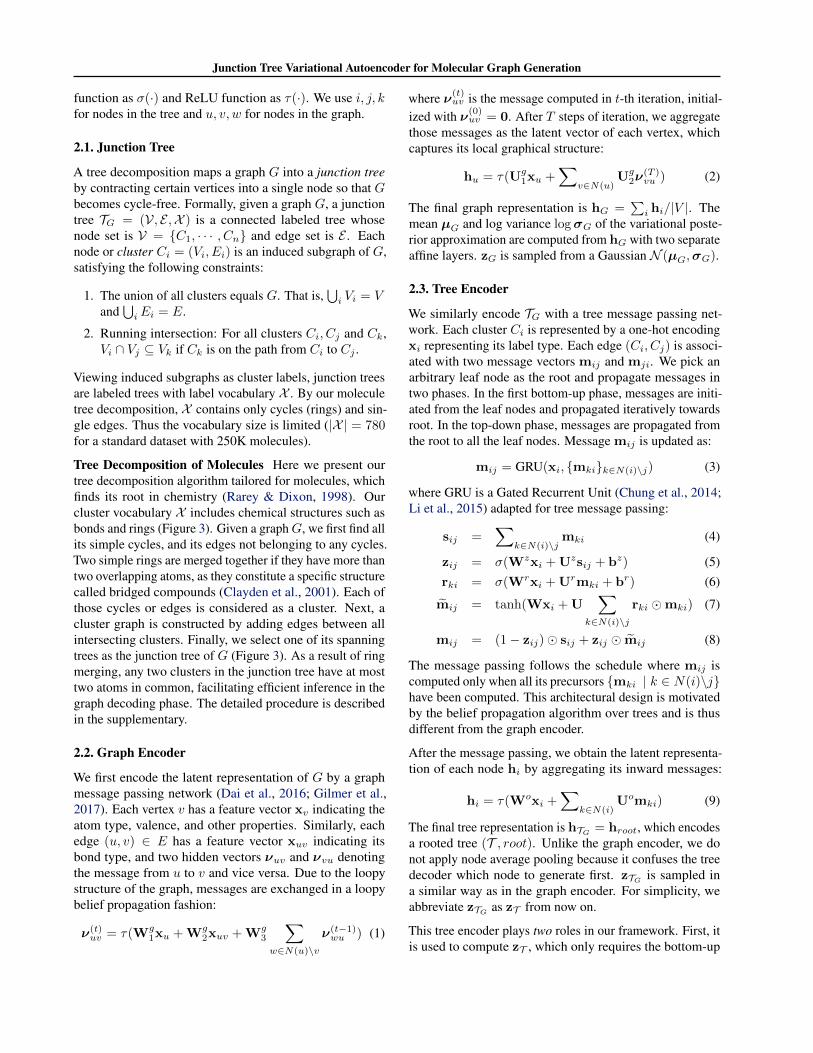
Figure 3. Overview of our method: A molecular graph G is firstdecomposed into its junction tree TG, where each colored node inthe tree represents a substructure in the molecule. We then encodeboth the tree and graph into their latent embeddings zT and zG.To decode the molecule, we first reconstruct junction tree from zT ,and then assemble nodes in the tree back to the original molecule.

of cliques is constrained a priori, we cannot guarantee thata junction tree exists with such clusters for an arbitrarymolecule. However, our clusters are built on the basis of themolecules in the training set to ensure that a correspondingjunction tree can be found. Empirically, our clusters covermost of the molecules in the test set.

The original molecular graph and its associated junction treeoffer two complementary representations of a molecule. Wetherefore encode the molecule into a two-part latent repre-sentation z = [zT , zG] where zT encodes the tree structureand what the clusters are in the tree without fully captur-ing how exactly the clusters are mutually connected. zGencodes the graph to capture the fine-grained connectivity.Both parts are created by tree and graph encoders q(zT |T )and q(zG|G). The latent representation is then decodedback into a molecular graph in two stages. As illustrated inFigure 3, we first reproduce the junction tree using a treedecoder p(T |zT ) based on the information in zT . Second,we predict the fine grain connectivity between the clustersin the junction tree using a graph decoder p(G|T , zG) torealize the full molecular graph. The junction tree approachallows us to maintain chemical feasibility during generation.

Notation A molecular graph is defined as G = (V,E)where V is the set of atoms (vertices) and E the set of bonds(edges). Let N(x) be the neighbor of x. We denote sigmoid

Junction Tree Variational Autoencoder for Molecular Graph Generation

function as σ(·) and ReLU function as τ(·). We use i, j, kfor nodes in the tree and u, v, w for nodes in the graph.

2.1. Junction Tree

A tree decomposition maps a graph G into a junction treeby contracting certain vertices into a single node so that Gbecomes cycle-free. Formally, given a graph G, a junctiontree TG = (V, E ,X ) is a connected labeled tree whosenode set is V = {C1, · · · , Cn} and edge set is E . Eachnode or cluster Ci = (Vi, Ei) is an induced subgraph of G,satisfying the following constraints:

1. The union of all clusters equals G. That is,⋃i Vi = V

and⋃iEi = E.

2. Running intersection: For all clusters Ci, Cj and Ck,Vi ∩ Vj ⊆ Vk if Ck is on the path from Ci to Cj .

Viewing induced subgraphs as cluster labels, junction treesare labeled trees with label vocabulary X . By our moleculetree decomposition, X contains only cycles (rings) and sin-gle edges. Thus the vocabulary size is limited (|X | = 780for a standard dataset with 250K molecules).

Tree Decomposition of Molecules Here we present ourtree decomposition algorithm tailored for molecules, whichfinds its root in chemistry (Rarey & Dixon, 1998). Ourcluster vocabulary X includes chemical structures such asbonds and rings (Figure 3). Given a graphG, we first find allits simple cycles, and its edges not belonging to any cycles.Two simple rings are merged together if they have more thantwo overlapping atoms, as they constitute a specific structurecalled bridged compounds (Clayden et al., 2001). Each ofthose cycles or edges is considered as a cluster. Next, acluster graph is constructed by adding edges between allintersecting clusters. Finally, we select one of its spanningtrees as the junction tree of G (Figure 3). As a result of ringmerging, any two clusters in the junction tree have at mosttwo atoms in common, facilitating efficient inference in thegraph decoding phase. The detailed procedure is describedin the supplementary.

2.2. Graph Encoder

We first encode the latent representation of G by a graphmessage passing network (Dai et al., 2016; Gilmer et al.,2017). Each vertex v has a feature vector xv indicating theatom type, valence, and other properties. Similarly, eachedge (u, v) ∈ E has a feature vector xuv indicating itsbond type, and two hidden vectors νuv and νvu denotingthe message from u to v and vice versa. Due to the loopystructure of the graph, messages are exchanged in a loopybelief propagation fashion:

ν(t)uv = τ(Wg

1xu +Wg2xuv +Wg

3

∑w∈N(u)\v

ν(t−1)wu ) (1)

where ν(t)uv is the message computed in t-th iteration, initial-

ized with ν(0)uv = 0. After T steps of iteration, we aggregate

those messages as the latent vector of each vertex, whichcaptures its local graphical structure:

hu = τ(Ug1xu +

∑v∈N(u)

Ug2ν

(T )vu ) (2)

The final graph representation is hG =∑i hi/|V |. The

mean µG and log variance logσG of the variational poste-rior approximation are computed from hG with two separateaffine layers. zG is sampled from a Gaussian N (µG,σG).

2.3. Tree Encoder

We similarly encode TG with a tree message passing net-work. Each cluster Ci is represented by a one-hot encodingxi representing its label type. Each edge (Ci, Cj) is associ-ated with two message vectors mij and mji. We pick anarbitrary leaf node as the root and propagate messages intwo phases. In the first bottom-up phase, messages are initi-ated from the leaf nodes and propagated iteratively towardsroot. In the top-down phase, messages are propagated fromthe root to all the leaf nodes. Message mij is updated as:

mij = GRU(xi, {mki}k∈N(i)\j) (3)

where GRU is a Gated Recurrent Unit (Chung et al., 2014;Li et al., 2015) adapted for tree message passing:

sij =∑

k∈N(i)\jmki (4)

zij = σ(Wzxi +Uzsij + bz) (5)rki = σ(Wrxi +Urmki + br) (6)

mij = tanh(Wxi +U∑

k∈N(i)\j

rki �mki) (7)

mij = (1− zij)� sij + zij � mij (8)

The message passing follows the schedule where mij iscomputed only when all its precursors {mki | k ∈ N(i)\j}have been computed. This architectural design is motivatedby the belief propagation algorithm over trees and is thusdifferent from the graph encoder.

After the message passing, we obtain the latent representa-tion of each node hi by aggregating its inward messages:

hi = τ(Woxi +∑

k∈N(i)Uomki) (9)

The final tree representation is hTG = hroot, which encodesa rooted tree (T , root). Unlike the graph encoder, we donot apply node average pooling because it confuses the treedecoder which node to generate first. zTG is sampled ina similar way as in the graph encoder. For simplicity, weabbreviate zTG as zT from now on.

This tree encoder plays two roles in our framework. First, itis used to compute zT , which only requires the bottom-up

Junction Tree Variational Autoencoder for Molecular Graph Generation

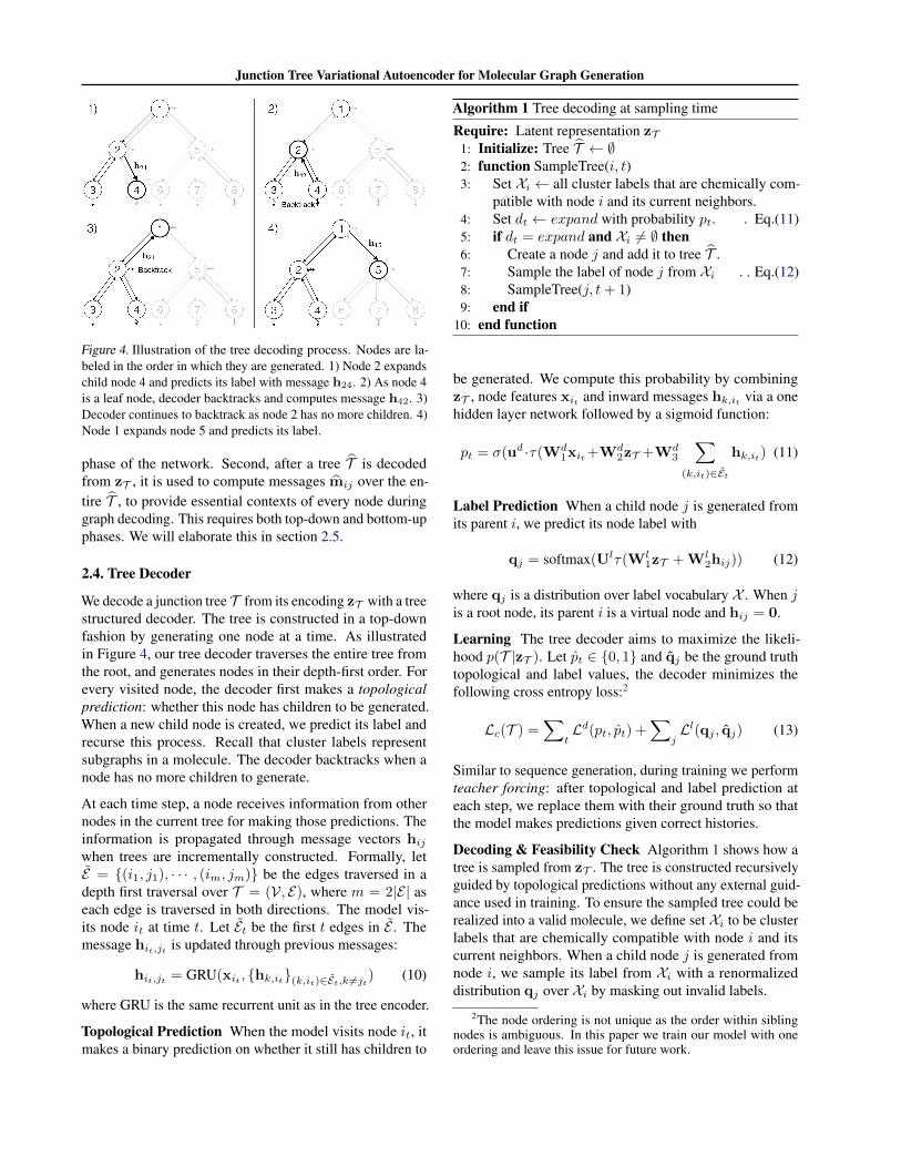
Figure 4. Illustration of the tree decoding process. Nodes are la-beled in the order in which they are generated. 1) Node 2 expandschild node 4 and predicts its label with message h24. 2) As node 4is a leaf node, decoder backtracks and computes message h42. 3)Decoder continues to backtrack as node 2 has no more children. 4)Node 1 expands node 5 and predicts its label.

phase of the network. Second, after a tree T is decodedfrom zT , it is used to compute messages mij over the en-tire T , to provide essential contexts of every node duringgraph decoding. This requires both top-down and bottom-upphases. We will elaborate this in section 2.5.

2.4. Tree Decoder

We decode a junction tree T from its encoding zT with a treestructured decoder. The tree is constructed in a top-downfashion by generating one node at a time. As illustratedin Figure 4, our tree decoder traverses the entire tree fromthe root, and generates nodes in their depth-first order. Forevery visited node, the decoder first makes a topologicalprediction: whether this node has children to be generated.When a new child node is created, we predict its label andrecurse this process. Recall that cluster labels representsubgraphs in a molecule. The decoder backtracks when anode has no more children to generate.

At each time step, a node receives information from othernodes in the current tree for making those predictions. Theinformation is propagated through message vectors hijwhen trees are incrementally constructed. Formally, letE = {(i1, j1), · · · , (im, jm)} be the edges traversed in adepth first traversal over T = (V, E), where m = 2|E| aseach edge is traversed in both directions. The model vis-its node it at time t. Let Et be the first t edges in E . Themessage hit,jt is updated through previous messages:

hit,jt = GRU(xit , {hk,it}(k,it)∈Et,k 6=jt) (10)

where GRU is the same recurrent unit as in the tree encoder.

Topological Prediction When the model visits node it, itmakes a binary prediction on whether it still has children to

Algorithm 1 Tree decoding at sampling time

Require: Latent representation zT1: Initialize: Tree T ← ∅2: function SampleTree(i, t)3: Set Xi ← all cluster labels that are chemically com-

patible with node i and its current neighbors.4: Set dt ← expand with probability pt. . Eq.(11)5: if dt = expand and Xi 6= ∅ then6: Create a node j and add it to tree T .7: Sample the label of node j from Xi .. Eq.(12)8: SampleTree(j, t+ 1)9: end if

10: end function

be generated. We compute this probability by combiningzT , node features xit and inward messages hk,it via a onehidden layer network followed by a sigmoid function:

pt = σ(ud ·τ(Wd1xit+Wd

2zT +Wd3

∑(k,it)∈Et

hk,it) (11)

Label Prediction When a child node j is generated fromits parent i, we predict its node label with

qj = softmax(Ulτ(Wl1zT +Wl

2hij)) (12)

where qj is a distribution over label vocabulary X . When jis a root node, its parent i is a virtual node and hij = 0.

Learning The tree decoder aims to maximize the likeli-hood p(T |zT ). Let pt ∈ {0, 1} and qj be the ground truthtopological and label values, the decoder minimizes thefollowing cross entropy loss:2

Lc(T ) =∑

tLd(pt, pt) +

∑jLl(qj , qj) (13)

Similar to sequence generation, during training we performteacher forcing: after topological and label prediction ateach step, we replace them with their ground truth so thatthe model makes predictions given correct histories.

Decoding & Feasibility Check Algorithm 1 shows how atree is sampled from zT . The tree is constructed recursivelyguided by topological predictions without any external guid-ance used in training. To ensure the sampled tree could berealized into a valid molecule, we define set Xi to be clusterlabels that are chemically compatible with node i and itscurrent neighbors. When a child node j is generated fromnode i, we sample its label from Xi with a renormalizeddistribution qj over Xi by masking out invalid labels.

2The node ordering is not unique as the order within siblingnodes is ambiguous. In this paper we train our model with oneordering and leave this issue for future work.

Junction Tree Variational Autoencoder for Molecular Graph Generation

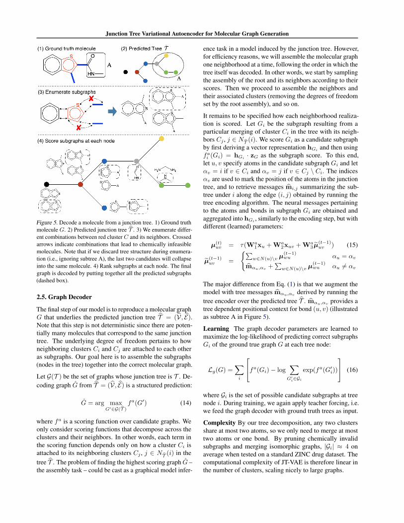
Figure 5. Decode a molecule from a junction tree. 1) Ground truthmolecule G. 2) Predicted junction tree T . 3) We enumerate differ-ent combinations between red cluster C and its neighbors. Crossedarrows indicate combinations that lead to chemically infeasiblemolecules. Note that if we discard tree structure during enumera-tion (i.e., ignoring subtree A), the last two candidates will collapseinto the same molecule. 4) Rank subgraphs at each node. The finalgraph is decoded by putting together all the predicted subgraphs(dashed box).

2.5. Graph Decoder

The final step of our model is to reproduce a molecular graphG that underlies the predicted junction tree T = (V, E).Note that this step is not deterministic since there are poten-tially many molecules that correspond to the same junctiontree. The underlying degree of freedom pertains to howneighboring clusters Ci and Cj are attached to each otheras subgraphs. Our goal here is to assemble the subgraphs(nodes in the tree) together into the correct molecular graph.

Let G(T ) be the set of graphs whose junction tree is T . De-coding graph G from T = (V, E) is a structured prediction:

G = arg maxG′∈G(T )

fa(G′) (14)

where fa is a scoring function over candidate graphs. Weonly consider scoring functions that decompose across theclusters and their neighbors. In other words, each term inthe scoring function depends only on how a cluster Ci isattached to its neighboring clusters Cj , j ∈ NT (i) in thetree T . The problem of finding the highest scoring graph G –the assembly task – could be cast as a graphical model infer-

ence task in a model induced by the junction tree. However,for efficiency reasons, we will assemble the molecular graphone neighborhood at a time, following the order in which thetree itself was decoded. In other words, we start by samplingthe assembly of the root and its neighbors according to theirscores. Then we proceed to assemble the neighbors andtheir associated clusters (removing the degrees of freedomset by the root assembly), and so on.

It remains to be specified how each neighborhood realiza-tion is scored. Let Gi be the subgraph resulting from aparticular merging of cluster Ci in the tree with its neigh-bors Cj , j ∈ NT (i). We score Gi as a candidate subgraphby first deriving a vector representation hGi

and then usingfai (Gi) = hGi

· zG as the subgraph score. To this end,let u, v specify atoms in the candidate subgraph Gi and letαv = i if v ∈ Ci and αv = j if v ∈ Cj \ Ci. The indicesαv are used to mark the position of the atoms in the junctiontree, and to retrieve messages mi,j summarizing the sub-tree under i along the edge (i, j) obtained by running thetree encoding algorithm. The neural messages pertainingto the atoms and bonds in subgraph Gi are obtained andaggregated into hGi

, similarly to the encoding step, but withdifferent (learned) parameters:

µ(t)uv = τ(Wa

1xu +Wa2xuv +Wa

3µ(t−1)uv ) (15)

µ(t−1)uv =

{∑w∈N(u)\v µ

(t−1)wu αu = αv

mαu,αv +∑w∈N(u)\v µ

(t−1)wu αu 6= αv

The major difference from Eq. (1) is that we augment themodel with tree messages mαu,αv derived by running thetree encoder over the predicted tree T . mαu,αv

provides atree dependent positional context for bond (u, v) (illustratedas subtree A in Figure 5).

Learning The graph decoder parameters are learned tomaximize the log-likelihood of predicting correct subgraphsGi of the ground true graph G at each tree node:

Lg(G) =∑i

fa(Gi)− log∑G′

i∈Gi

exp(fa(G′i))

(16)

where Gi is the set of possible candidate subgraphs at treenode i. During training, we again apply teacher forcing, i.e.we feed the graph decoder with ground truth trees as input.

Complexity By our tree decomposition, any two clustersshare at most two atoms, so we only need to merge at mosttwo atoms or one bond. By pruning chemically invalidsubgraphs and merging isomorphic graphs, |Gi| ≈ 4 onaverage when tested on a standard ZINC drug dataset. Thecomputational complexity of JT-VAE is therefore linear inthe number of clusters, scaling nicely to large graphs.

Junction Tree Variational Autoencoder for Molecular Graph Generation

NH

O

N

S

O HS

O

O

NH

O

H3N+

NNH O

O-

N

O

NNH+

NH

O

N

NH

Cl

NH2+

NH

O

N

S

O

O

N

S

O

NH

S

N

H

O

O

N

NN

O

O

N

N

N

NCl

NHO

N

F

NO

N

O

NO

H2N

NH

ON

O

N

NH+

NH

O

N

S

N

N

O

O

NH

S

NH3+

NH

O

O

S

O

O

O

S

O

NH

N

OH

N

O

NH

NH2

O

NHN

O

NH

O

O

H2N

NH

SO

O

O

O

NH

O

O

O

NH

N

N

N

OH

SN

N

O

NH2+

O

O

NN

NHO

NH+ N

O

S

O O

N

O

H

H

NH2

N

O

NH

O

NH

N

S

N

N

Cl

NO

N

OH

SNH

O

N

NH

N

N N

N

H

HNH

N

N N

N

H

H

N N

N

N

NHHNH2

+

NH

N

NN

N

NH

N

N N

N

NH2+

NH

N

N N

N

NH2+

NH

N

N N

N

NH

N

N N

N

NH

N

N

N

N

NH

N

N N

N

NH

N

N N

N

NH

N

N N

N

NH

N

NN

N

N

N

N

N

NH

S

O

N

N

N

N

NH

S

O

NH

S

O

N

N

N

N

NH

N

N N

N

NH

N

N N

N

NH

N

N N

N

NH

N

N N

N

NH

N

NN

N

NH

N

NN

N

NH

N

NN

N

NH

N

NN

N

NH

S

ON

N

N

N

NH

S

ON

N

N

N

NH

S

ON

N

N

N

NH

N

N

N

N

NH

N

N

N

NNH

N

NN

N

NH

N

NN

N

NH

N

NN

N

NH

N

NN

N

NH

N

NN

N

NH

N

NN

N

NH

S

ON

N

N

N

NHN

H2N

S

N

NH

N

N

N

NNH

N

NN

N

NH

N

NN

N

NH

N

NN

N

NH

N

NN

N

NH

N

NN

N

NH

N

NN

N

NH

N

NN

N

NH N

NH2

S

N

S

NH N

NH2

S

N

SNH

N

NN

N

NH

N

NN

N

NH

N

NN

N

NH

N

NN

N

NH

N

NN

N

NH

N

NN

N

NH

N

NN

N

NH N

NH2

S

N

S

NH N

NH2

S

N

S

N

NHN

NH 2

S

S

NH

N

NN

N

NH

N

NN

N

NH

N

NN

N

NH

N

NN

N

NH

N

NN

N

N

N

S

NN

NH2

NH

NH+

NH

N

NH2S

N

ONH2

+ N

NH

N

NH

2

S

S

N

NH

N

NH

2

S

S

N

NH

N

NH2

S

S

NH

N

NN

N

NH

N

NN

N

NH

N

N

N

N

N

N

S

NN

N

NH+

N

N

S

NN

NH2

NH

NH+

NH

N

NH2S

N

ONH2

+

NH

N

NH2S

N

ONH2

+

N

NHN

H2N

S S

N

NHN

H2N

S S

N

NH

N

NH

2

S

S NH

N

N

N

N

NH

N

N

N

N

NH+

N

N

S

NN

NH2

NH

NH+

N

N

S

NN

NH2

NH

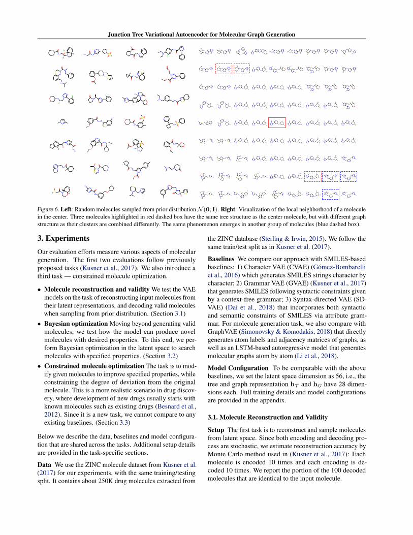
Figure 6. Left: Random molecules sampled from prior distributionN (0, I). Right: Visualization of the local neighborhood of a moleculein the center. Three molecules highlighted in red dashed box have the same tree structure as the center molecule, but with different graphstructure as their clusters are combined differently. The same phenomenon emerges in another group of molecules (blue dashed box).

3. ExperimentsOur evaluation efforts measure various aspects of moleculargeneration. The first two evaluations follow previouslyproposed tasks (Kusner et al., 2017). We also introduce athird task — constrained molecule optimization.

• Molecule reconstruction and validity We test the VAEmodels on the task of reconstructing input molecules fromtheir latent representations, and decoding valid moleculeswhen sampling from prior distribution. (Section 3.1)• Bayesian optimization Moving beyond generating valid

molecules, we test how the model can produce novelmolecules with desired properties. To this end, we per-form Bayesian optimization in the latent space to searchmolecules with specified properties. (Section 3.2)

• Constrained molecule optimization The task is to mod-ify given molecules to improve specified properties, whileconstraining the degree of deviation from the originalmolecule. This is a more realistic scenario in drug discov-ery, where development of new drugs usually starts withknown molecules such as existing drugs (Besnard et al.,2012). Since it is a new task, we cannot compare to anyexisting baselines. (Section 3.3)

Below we describe the data, baselines and model configura-tion that are shared across the tasks. Additional setup detailsare provided in the task-specific sections.

Data We use the ZINC molecule dataset from Kusner et al.(2017) for our experiments, with the same training/testingsplit. It contains about 250K drug molecules extracted from

the ZINC database (Sterling & Irwin, 2015). We follow thesame train/test split as in Kusner et al. (2017).

Baselines We compare our approach with SMILES-basedbaselines: 1) Character VAE (CVAE) (Gomez-Bombarelliet al., 2016) which generates SMILES strings character bycharacter; 2) Grammar VAE (GVAE) (Kusner et al., 2017)that generates SMILES following syntactic constraints givenby a context-free grammar; 3) Syntax-directed VAE (SD-VAE) (Dai et al., 2018) that incorporates both syntacticand semantic constraints of SMILES via attribute gram-mar. For molecule generation task, we also compare withGraphVAE (Simonovsky & Komodakis, 2018) that directlygenerates atom labels and adjacency matrices of graphs, aswell as an LSTM-based autoregressive model that generatesmolecular graphs atom by atom (Li et al., 2018).

Model Configuration To be comparable with the abovebaselines, we set the latent space dimension as 56, i.e., thetree and graph representation hT and hG have 28 dimen-sions each. Full training details and model configurationsare provided in the appendix.

3.1. Molecule Reconstruction and Validity

Setup The first task is to reconstruct and sample moleculesfrom latent space. Since both encoding and decoding pro-cess are stochastic, we estimate reconstruction accuracy byMonte Carlo method used in (Kusner et al., 2017): Eachmolecule is encoded 10 times and each encoding is de-coded 10 times. We report the portion of the 100 decodedmolecules that are identical to the input molecule.

Junction Tree Variational Autoencoder for Molecular Graph Generation

Table 1. Reconstruction accuracy and prior validity results. Base-line results are copied from Kusner et al. (2017); Dai et al. (2018);Simonovsky & Komodakis (2018); Li et al. (2018).

Method Reconstruction ValidityCVAE 44.6% 0.7%GVAE 53.7% 7.2%SD-VAE 76.2% 43.5%GraphVAE - 13.5%Atom-by-Atom LSTM - 89.2%JT-VAE 76.7% 100.0%

To compute validity, we sample 1000 latent vectors fromthe prior distribution N (0, I), and decode each of thesevectors 100 times. We report the percentage of decodedmolecules that are chemically valid (checked by RDKit).For ablation study, we also report the validity of our modelwithout validity check in decoding phase.

Results Table 1 shows that JT-VAE outperforms previousmodels in molecule reconstruction, and always producesvalid molecules when sampled from prior distribution. Incontrast, the atom-by-atom based generation only achieves89.2% validity as it needs to go through invalid intermediatestates (Figure 2). Our model bypasses this issue by utilizingvalid substructures as building blocks. As shown in Figure 6,the sampled molecules have non-trivial structures such assimple chains. We further sampled 5000 molecules fromprior and found they are all distinct from the training set.Thus our model is not a simple memorization.

Analysis We qualitatively examine the latent space of JT-VAE by visualizing the neighborhood of molecules. Givena molecule, we follow the method in Kusner et al. (2017)to construct a grid visualization of its neighborhood. Fig-ure 6 shows the local neighborhood of the same moleculevisualized in Dai et al. (2018). In comparison, our neighbor-hood does not contain molecules with huge rings (with morethan 7 atoms), which rarely occur in the dataset. We alsohighlight two groups of closely resembling molecules thathave identical tree structures but vary only in how clustersare attached together. This demonstrates the smoothness oflearned molecular embeddings.

3.2. Bayesian Optimization

Setup The second task is to produce novel molecules withdesired properties. Following (Kusner et al., 2017), ourtarget chemical property y(·) is octanol-water partition coef-ficients (logP) penalized by the synthetic accessibility (SA)score and number of long cycles.3 To perform Bayesianoptimization (BO), we first train a VAE and associate each

3y(m) = logP (m) − SA(m) − cycle(m) where cycle(m)counts the number of rings that have more than six atoms.

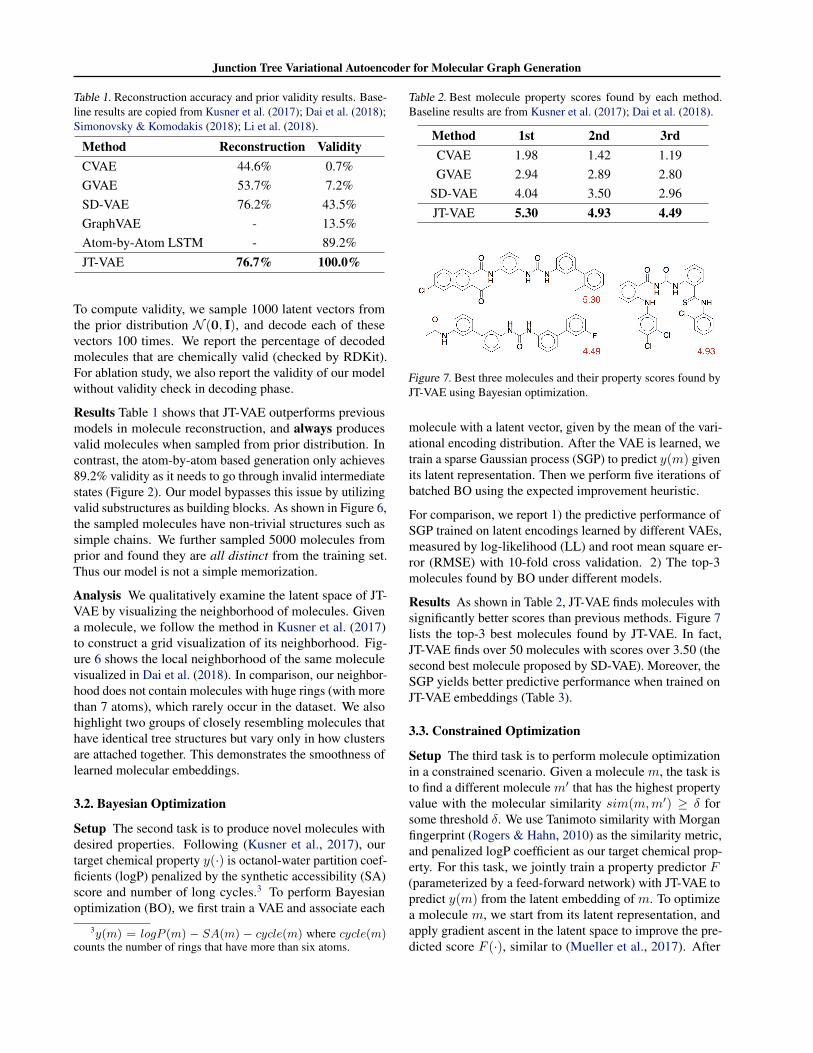
Table 2. Best molecule property scores found by each method.Baseline results are from Kusner et al. (2017); Dai et al. (2018).

Method 1st 2nd 3rdCVAE 1.98 1.42 1.19GVAE 2.94 2.89 2.80

SD-VAE 4.04 3.50 2.96JT-VAE 5.30 4.93 4.49

Figure 7. Best three molecules and their property scores found byJT-VAE using Bayesian optimization.

molecule with a latent vector, given by the mean of the vari-ational encoding distribution. After the VAE is learned, wetrain a sparse Gaussian process (SGP) to predict y(m) givenits latent representation. Then we perform five iterations ofbatched BO using the expected improvement heuristic.

For comparison, we report 1) the predictive performance ofSGP trained on latent encodings learned by different VAEs,measured by log-likelihood (LL) and root mean square er-ror (RMSE) with 10-fold cross validation. 2) The top-3molecules found by BO under different models.

Results As shown in Table 2, JT-VAE finds molecules withsignificantly better scores than previous methods. Figure 7lists the top-3 best molecules found by JT-VAE. In fact,JT-VAE finds over 50 molecules with scores over 3.50 (thesecond best molecule proposed by SD-VAE). Moreover, theSGP yields better predictive performance when trained onJT-VAE embeddings (Table 3).

3.3. Constrained Optimization

Setup The third task is to perform molecule optimizationin a constrained scenario. Given a molecule m, the task isto find a different molecule m′ that has the highest propertyvalue with the molecular similarity sim(m,m′) ≥ δ forsome threshold δ. We use Tanimoto similarity with Morganfingerprint (Rogers & Hahn, 2010) as the similarity metric,and penalized logP coefficient as our target chemical prop-erty. For this task, we jointly train a property predictor F(parameterized by a feed-forward network) with JT-VAE topredict y(m) from the latent embedding of m. To optimizea molecule m, we start from its latent representation, andapply gradient ascent in the latent space to improve the pre-dicted score F (·), similar to (Mueller et al., 2017). After

Junction Tree Variational Autoencoder for Molecular Graph Generation

Table 3. Predictive performance of sparse Gaussian Processestrained on different VAEs. Baseline results are copied from Kusneret al. (2017) and Dai et al. (2018).

Method LL RMSECVAE −1.812± 0.004 1.504± 0.006

GVAE −1.739± 0.004 1.404± 0.006

SD-VAE −1.697± 0.015 1.366± 0.023

JT-VAE −1.658± 0.023 1.290± 0.026

Table 4. Constrained optimization result of JT-VAE: mean andstandard deviation of property improvement, molecular similarityand success rate under constraints sim(m,m′) ≥ δ with varied δ.

δ Improvement Similarity Success0.0 1.91± 2.04 0.28± 0.15 97.5%0.2 1.68± 1.85 0.33± 0.13 97.1%0.4 0.84± 1.45 0.51± 0.10 83.6%0.6 0.21± 0.71 0.69± 0.06 46.4%

applying K = 80 gradient steps, K molecules are decodedfrom resulting latent trajectories, and we report the moleculewith the highest F (·) that satisfies the similarity constraint.A modification succeeds if one of the decoded moleculessatisfies the constraint and is distinct from the original.

To provide the greatest challenge, we selected 800 moleculeswith the lowest property score y(·) from the test set. Wereport the success rate (how often a modification succeeds),and among success cases the average improvement y(m′)−y(m) and molecular similarity sim(m,m′) between theoriginal and modified molecules m and m′.

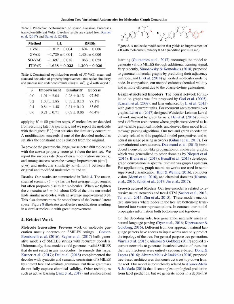
Results Our results are summarized in Table 4. The uncon-strained scenario (δ = 0) has the best average improvement,but often proposes dissimilar molecules. When we tightenthe constraint to δ = 0.4, about 80% of the time our modelfinds similar molecules, with an average improvement 0.84.This also demonstrates the smoothness of the learned latentspace. Figure 8 illustrates an effective modification resultingin a similar molecule with great improvement.

4. Related WorkMolecule Generation Previous work on molecule gen-eration mostly operates on SMILES strings. Gomez-Bombarelli et al. (2016); Segler et al. (2017) built gener-ative models of SMILES strings with recurrent decoders.Unfortunately, these models could generate invalid SMILESthat do not result in any molecules. To remedy this issue,Kusner et al. (2017); Dai et al. (2018) complemented thedecoder with syntactic and semantic constraints of SMILESby context free and attribute grammars, but these grammarsdo not fully capture chemical validity. Other techniquessuch as active learning (Janz et al., 2017) and reinforcement

Figure 8. A molecule modification that yields an improvement of4.0 with molecular similarity 0.617 (modified part is in red).

learning (Guimaraes et al., 2017) encourage the model togenerate valid SMILES through additional training signal.Very recently, Simonovsky & Komodakis (2018) proposedto generate molecular graphs by predicting their adjacencymatrices, and Li et al. (2018) generated molecules node bynode. In comparison, our method enforces chemical validityand is more efficient due to the coarse-to-fine generation.

Graph-structured Encoders The neural network formu-lation on graphs was first proposed by Gori et al. (2005);Scarselli et al. (2009), and later enhanced by Li et al. (2015)with gated recurrent units. For recurrent architectures overgraphs, Lei et al. (2017) designed Weisfeiler-Lehman kernelnetwork inspired by graph kernels. Dai et al. (2016) consid-ered a different architecture where graphs were viewed as la-tent variable graphical models, and derived their model frommessage passing algorithms. Our tree and graph encoder areclosely related to this graphical model perspective, and toneural message passing networks (Gilmer et al., 2017). Forconvolutional architectures, Duvenaud et al. (2015) intro-duced a convolution-like propagation on molecular graphs,which was generalized to other domains by Niepert et al.(2016). Bruna et al. (2013); Henaff et al. (2015) developedgraph convolution in spectral domain via graph Laplacian.For applications, graph neural networks are used in semi-supervised classification (Kipf & Welling, 2016), computervision (Monti et al., 2016), and chemical domains (Kearneset al., 2016; Schutt et al., 2017; Jin et al., 2017).

Tree-structured Models Our tree encoder is related to re-cursive neural networks and tree-LSTM (Socher et al., 2013;Tai et al., 2015; Zhu et al., 2015). These models encodetree structures where nodes in the tree are bottom-up trans-formed into vector representations. In contrast, our modelpropagates information both bottom-up and top-down.

On the decoding side, tree generation naturally arises innatural language parsing (Dyer et al., 2016; Kiperwasser &Goldberg, 2016). Different from our approach, natural lan-guage parsers have access to input words and only predictthe topology of the tree. For general purpose tree generation,Vinyals et al. (2015); Aharoni & Goldberg (2017) applied re-current networks to generate linearized version of trees, buttheir architectures were entirely sequence-based. Dong &Lapata (2016); Alvarez-Melis & Jaakkola (2016) proposedtree-based architectures that construct trees top-down fromthe root. Our model is most closely related to Alvarez-Melis& Jaakkola (2016) that disentangles topological predictionfrom label prediction, but we generate nodes in a depth-first

Junction Tree Variational Autoencoder for Molecular Graph Generation

order and have additional steps that propagate informationbottom-up. This forward-backward propagation also ap-pears in Parisotto et al. (2016), but their model is nodebased whereas ours is based on message passing.

5. ConclusionIn this paper we present a junction tree variational autoen-coder for generating molecular graphs. Our method signifi-cantly outperforms previous work in molecule generationand optimization. For future work, we attempt to generalizeour method for general low-treewidth graphs.

AcknowledgementWe thank Jonas Mueller, Chengtao Li, Tao Lei and MITNLP Group for their helpful comments. This work wassupported by the DARPA Make-It program under contractARO W911NF-16-2-0023.

ReferencesAharoni, R. and Goldberg, Y. Towards string-to-tree neural

machine translation. arXiv preprint arXiv:1704.04743,2017.

Alvarez-Melis, D. and Jaakkola, T. S. Tree-structured de-coding with doubly-recurrent neural networks. 2016.

Besnard, J., Ruda, G. F., Setola, V., Abecassis, K., Ro-driguiz, R. M., Huang, X.-P., Norval, S., Sassano, M. F.,Shin, A. I., Webster, L. A., et al. Automated design of lig-ands to polypharmacological profiles. Nature, 492(7428):215–220, 2012.

Bruna, J., Zaremba, W., Szlam, A., and LeCun, Y. Spec-tral networks and locally connected networks on graphs.arXiv preprint arXiv:1312.6203, 2013.

Chung, J., Gulcehre, C., Cho, K., and Bengio, Y. Empiricalevaluation of gated recurrent neural networks on sequencemodeling. arXiv preprint arXiv:1412.3555, 2014.

Clayden, J., Greeves, N., Warren, S., and Wothers, P. Or-ganic Chemistry. Oxford University Press, 2001.

Dai, H., Dai, B., and Song, L. Discriminative embeddings oflatent variable models for structured data. In InternationalConference on Machine Learning, pp. 2702–2711, 2016.

Dai, H., Tian, Y., Dai, B., Skiena, S., and Song, L. Syntax-directed variational autoencoder for structured data. In-ternational Conference on Learning Representations,2018. URL https://openreview.net/forum?id=SyqShMZRb.

Dong, L. and Lapata, M. Language to logical form withneural attention. arXiv preprint arXiv:1601.01280, 2016.

Duvenaud, D. K., Maclaurin, D., Iparraguirre, J., Bombarell,R., Hirzel, T., Aspuru-Guzik, A., and Adams, R. P. Con-volutional networks on graphs for learning molecular fin-gerprints. In Advances in neural information processingsystems, pp. 2224–2232, 2015.

Dyer, C., Kuncoro, A., Ballesteros, M., and Smith, N. A.Recurrent neural network grammars. arXiv preprintarXiv:1602.07776, 2016.

Gilmer, J., Schoenholz, S. S., Riley, P. F., Vinyals, O., andDahl, G. E. Neural message passing for quantum chem-istry. arXiv preprint arXiv:1704.01212, 2017.

Gomez-Bombarelli, R., Wei, J. N., Duvenaud, D.,Hernandez-Lobato, J. M., Sanchez-Lengeling, B., She-berla, D., Aguilera-Iparraguirre, J., Hirzel, T. D., Adams,R. P., and Aspuru-Guzik, A. Automatic chemical de-sign using a data-driven continuous representation ofmolecules. ACS Central Science, 2016. doi: 10.1021/acscentsci.7b00572.

Gori, M., Monfardini, G., and Scarselli, F. A new modelfor learning in graph domains. In Neural Networks, 2005.IJCNN’05. Proceedings. 2005 IEEE International JointConference on, volume 2, pp. 729–734. IEEE, 2005.

Guimaraes, G. L., Sanchez-Lengeling, B., Farias, P. L. C.,and Aspuru-Guzik, A. Objective-reinforced generative ad-versarial networks (organ) for sequence generation mod-els. arXiv preprint arXiv:1705.10843, 2017.

Henaff, M., Bruna, J., and LeCun, Y. Deep convolu-tional networks on graph-structured data. arXiv preprintarXiv:1506.05163, 2015.

Janz, D., van der Westhuizen, J., and Hernandez-Lobato,J. M. Actively learning what makes a discrete sequencevalid. arXiv preprint arXiv:1708.04465, 2017.

Jin, W., Coley, C., Barzilay, R., and Jaakkola, T. Predict-ing organic reaction outcomes with weisfeiler-lehmannetwork. In Advances in Neural Information ProcessingSystems, pp. 2604–2613, 2017.

Kearnes, S., McCloskey, K., Berndl, M., Pande, V., andRiley, P. Molecular graph convolutions: moving beyondfingerprints. Journal of computer-aided molecular design,30(8):595–608, 2016.

Kingma, D. P. and Welling, M. Auto-encoding variationalbayes. arXiv preprint arXiv:1312.6114, 2013.

Kiperwasser, E. and Goldberg, Y. Easy-first dependencyparsing with hierarchical tree lstms. arXiv preprintarXiv:1603.00375, 2016.

Junction Tree Variational Autoencoder for Molecular Graph Generation

Kipf, T. N. and Welling, M. Semi-supervised classifica-tion with graph convolutional networks. arXiv preprintarXiv:1609.02907, 2016.

Kusner, M. J., Paige, B., and Hernandez-Lobato, J. M.Grammar variational autoencoder. arXiv preprintarXiv:1703.01925, 2017.

Landrum, G. Rdkit: Open-source cheminformatics. Online).http://www. rdkit. org. Accessed, 3(04):2012, 2006.

Lei, T., Jin, W., Barzilay, R., and Jaakkola, T. Derivingneural architectures from sequence and graph kernels.arXiv preprint arXiv:1705.09037, 2017.

Li, Y., Tarlow, D., Brockschmidt, M., and Zemel, R.Gated graph sequence neural networks. arXiv preprintarXiv:1511.05493, 2015.

Li, Y., Vinyals, O., Dyer, C., Pascanu, R., and Battaglia,P. Learning deep generative models of graphs. arXivpreprint arXiv:1803.03324, 2018.

Monti, F., Boscaini, D., Masci, J., Rodola, E., Svoboda, J.,and Bronstein, M. M. Geometric deep learning on graphsand manifolds using mixture model cnns. arXiv preprintarXiv:1611.08402, 2016.

Mueller, J., Gifford, D., and Jaakkola, T. Sequence to bettersequence: continuous revision of combinatorial structures.In International Conference on Machine Learning, pp.2536–2544, 2017.

Niepert, M., Ahmed, M., and Kutzkov, K. Learning con-volutional neural networks for graphs. In InternationalConference on Machine Learning, pp. 2014–2023, 2016.

Parisotto, E., Mohamed, A.-r., Singh, R., Li, L., Zhou, D.,and Kohli, P. Neuro-symbolic program synthesis. arXivpreprint arXiv:1611.01855, 2016.

Rarey, M. and Dixon, J. S. Feature trees: a new molecularsimilarity measure based on tree matching. Journal ofcomputer-aided molecular design, 12(5):471–490, 1998.

Rogers, D. and Hahn, M. Extended-connectivity finger-prints. Journal of chemical information and modeling, 50(5):742–754, 2010.

Scarselli, F., Gori, M., Tsoi, A. C., Hagenbuchner, M., andMonfardini, G. The graph neural network model. IEEETransactions on Neural Networks, 20(1):61–80, 2009.

Schutt, K., Kindermans, P.-J., Felix, H. E. S., Chmiela, S.,Tkatchenko, A., and Muller, K.-R. Schnet: A continuous-filter convolutional neural network for modeling quantuminteractions. In Advances in Neural Information Process-ing Systems, pp. 992–1002, 2017.

Segler, M. H., Kogej, T., Tyrchan, C., and Waller, M. P.Generating focussed molecule libraries for drug dis-covery with recurrent neural networks. arXiv preprintarXiv:1701.01329, 2017.

Simonovsky, M. and Komodakis, N. Graphvae: Towardsgeneration of small graphs using variational autoencoders.arXiv preprint arXiv:1802.03480, 2018.

Socher, R., Perelygin, A., Wu, J., Chuang, J., Manning,C. D., Ng, A., and Potts, C. Recursive deep models forsemantic compositionality over a sentiment treebank. InProceedings of the 2013 conference on empirical methodsin natural language processing, pp. 1631–1642, 2013.

Sterling, T. and Irwin, J. J. Zinc 15–ligand discovery foreveryone. J. Chem. Inf. Model, 55(11):2324–2337, 2015.

Tai, K. S., Socher, R., and Manning, C. D. Improved seman-tic representations from tree-structured long short-termmemory networks. arXiv preprint arXiv:1503.00075,2015.

Vinyals, O., Kaiser, Ł., Koo, T., Petrov, S., Sutskever, I.,and Hinton, G. Grammar as a foreign language. InAdvances in Neural Information Processing Systems, pp.2773–2781, 2015.

Weininger, D. Smiles, a chemical language and informationsystem. 1. introduction to methodology and encodingrules. Journal of chemical information and computersciences, 28(1):31–36, 1988.

Zhu, X., Sobihani, P., and Guo, H. Long short-term memoryover recursive structures. In International Conference onMachine Learning, pp. 1604–1612, 2015.

Supplementary Material

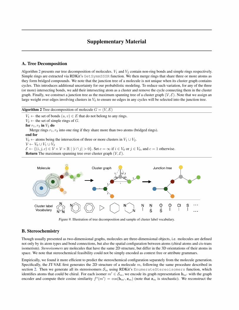
A. Tree DecompositionAlgorithm 2 presents our tree decomposition of molecules. V1 and V2 contain non-ring bonds and simple rings respectively.Simple rings are extracted via RDKit’s GetSymmSSSR function. We then merge rings that share three or more atoms asthey form bridged compounds. We note that the junction tree of a molecule is not unique when its cluster graph containscycles. This introduces additional uncertainty for our probabilistic modeling. To reduce such variation, for any of the three(or more) intersecting bonds, we add their intersecting atom as a cluster and remove the cycle connecting them in the clustergraph. Finally, we construct a junction tree as the maximum spanning tree of a cluster graph (V, E). Note that we assign anlarge weight over edges involving clusters in V0 to ensure no edges in any cycles will be selected into the junction tree.

Algorithm 2 Tree decomposition of molecule G = (V,E)

V1 ← the set of bonds (u, v) ∈ E that do not belong to any rings.V2 ← the set of simple rings of G.for r1, r2 in V2 do

Merge rings r1, r2 into one ring if they share more than two atoms (bridged rings).end forV0 ← atoms being the intersection of three or more clusters in V1 ∪ V2.V ← V0 ∪ V1 ∪ V2E ← {(i, j, c) ∈ V × V × R | |i ∩ j| > 0}. Set c =∞ if i ∈ V0 or j ∈ V0, and c = 1 otherwise.Return The maximum spanning tree over cluster graph (V, E).

Figure 9. Illustration of tree decomposition and sample of cluster label vocabulary.

B. StereochemistryThough usually presented as two-dimensional graphs, molecules are three-dimensional objects, i.e. molecules are definednot only by its atom types and bond connections, but also the spatial configuration between atoms (chiral atoms and cis-transisomerism). Stereoisomers are molecules that have the same 2D structure, but differ in the 3D orientations of their atoms inspace. We note that stereochemical feasibility could not be simply encoded as context free or attribute grammars.

Empirically, we found it more efficient to predict the stereochemical configuration separately from the molecule generation.Specifically, the JT-VAE first generates the 2D structure of a molecule m, following the same procedure described insection 2. Then we generate all its stereoisomers Sm using RDKit’s EnumerateStereoisomers function, whichidentifies atoms that could be chiral. For each isomer m′ ∈ Sm, we encode its graph representation hm′ with the graphencoder and compute their cosine similarity fs(m′) = cos(hm′ , zm) (note that zm is stochastic). We reconstruct the

Junction Tree Variational Autoencoder for Molecular Graph Generation

final 3D structure by picking the stereoisomer m = argmaxm′ fs(m′). Since on average only few atoms could havestereochemical variations, this post ranking process is very efficient. Combining this with tree and graph generation, themolecule reconstruction loss L becomes

L = Lc + Lg + Ls; Ls = fs(m)− log∑

m′∈Sm

exp(fs(m′)) (17)

C. Training DetailsBy applying tree decomposition over 240K molecules in ZINC dataset, we collected our vocabulary set X of size |X | = 780.The hidden state dimension is 450 for all modules in JT-VAE and the latent bottleneck dimension is 56. For the graphencoder, the initial atom features include its atom type, degree, its formal charge and its chiral configuration. Bond feature isa concatenation of its bond type, whether the bond is in a ring, and its cis-trans configuration. For our tree encoder, werepresent each cluster with a neural embedding vector, similar to word embedding for words. The tree and graph decoderuse the same feature setting as encoders. The graph encoder and decoder runs three iterations of neural message passing.For fair comparison to SMILES based method, we minimized feature engineering. We use PyTorch to implement all neuralcomponents and RDKit to process molecules.

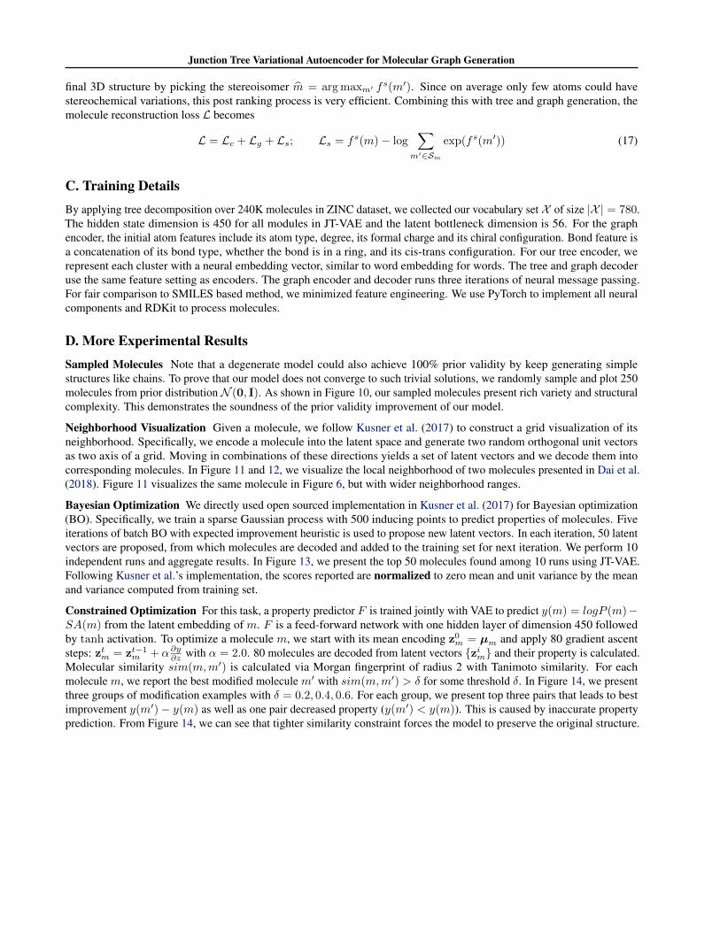
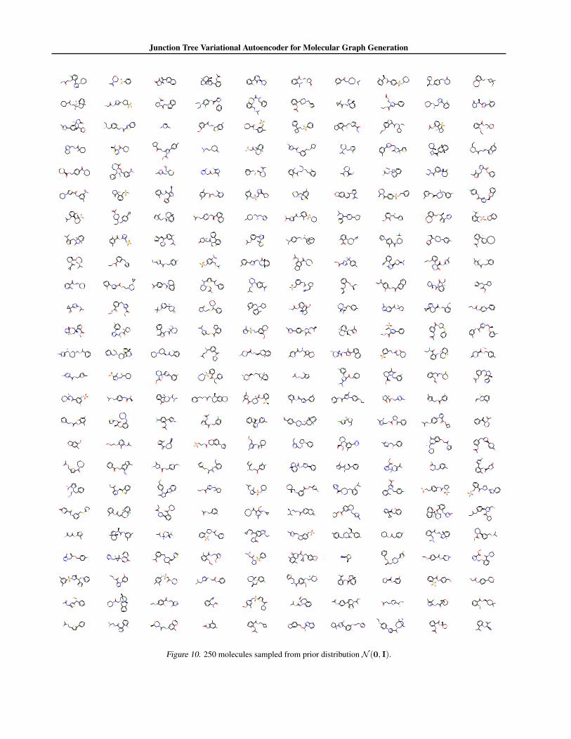
D. More Experimental ResultsSampled Molecules Note that a degenerate model could also achieve 100% prior validity by keep generating simplestructures like chains. To prove that our model does not converge to such trivial solutions, we randomly sample and plot 250molecules from prior distributionN (0, I). As shown in Figure 10, our sampled molecules present rich variety and structuralcomplexity. This demonstrates the soundness of the prior validity improvement of our model.

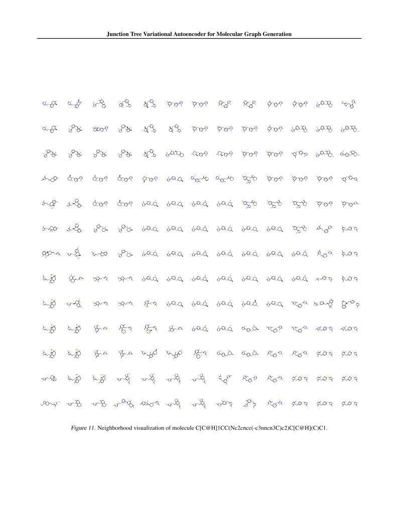
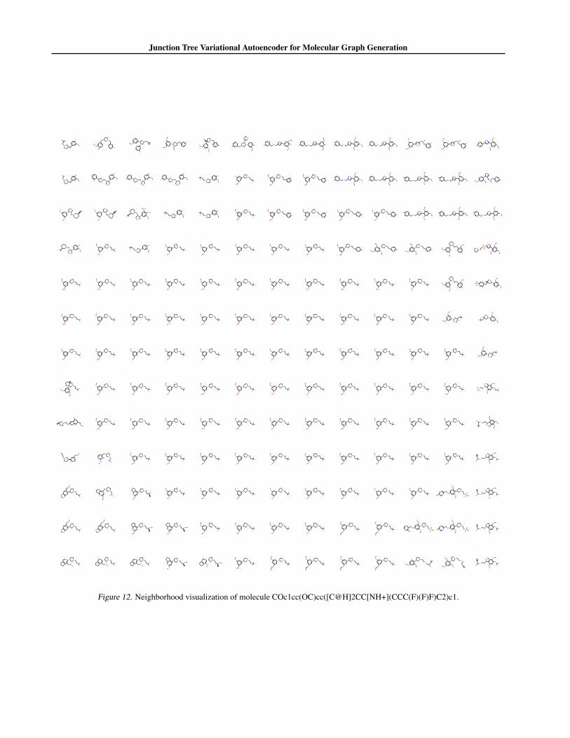
Neighborhood Visualization Given a molecule, we follow Kusner et al. (2017) to construct a grid visualization of itsneighborhood. Specifically, we encode a molecule into the latent space and generate two random orthogonal unit vectorsas two axis of a grid. Moving in combinations of these directions yields a set of latent vectors and we decode them intocorresponding molecules. In Figure 11 and 12, we visualize the local neighborhood of two molecules presented in Dai et al.(2018). Figure 11 visualizes the same molecule in Figure 6, but with wider neighborhood ranges.

Bayesian Optimization We directly used open sourced implementation in Kusner et al. (2017) for Bayesian optimization(BO). Specifically, we train a sparse Gaussian process with 500 inducing points to predict properties of molecules. Fiveiterations of batch BO with expected improvement heuristic is used to propose new latent vectors. In each iteration, 50 latentvectors are proposed, from which molecules are decoded and added to the training set for next iteration. We perform 10independent runs and aggregate results. In Figure 13, we present the top 50 molecules found among 10 runs using JT-VAE.Following Kusner et al.’s implementation, the scores reported are normalized to zero mean and unit variance by the meanand variance computed from training set.

Constrained Optimization For this task, a property predictor F is trained jointly with VAE to predict y(m) = logP (m)−SA(m) from the latent embedding of m. F is a feed-forward network with one hidden layer of dimension 450 followedby tanh activation. To optimize a molecule m, we start with its mean encoding z0m = µm and apply 80 gradient ascentsteps: ztm = zt−1m + α∂y∂z with α = 2.0. 80 molecules are decoded from latent vectors {zim} and their property is calculated.Molecular similarity sim(m,m′) is calculated via Morgan fingerprint of radius 2 with Tanimoto similarity. For eachmolecule m, we report the best modified molecule m′ with sim(m,m′) > δ for some threshold δ. In Figure 14, we presentthree groups of modification examples with δ = 0.2, 0.4, 0.6. For each group, we present top three pairs that leads to bestimprovement y(m′)− y(m) as well as one pair decreased property (y(m′) < y(m)). This is caused by inaccurate propertyprediction. From Figure 14, we can see that tighter similarity constraint forces the model to preserve the original structure.

Junction Tree Variational Autoencoder for Molecular Graph Generation

NH

O

O

Cl

N

N

N

N

O

N

O

S

O

N

NH2

NH

O

OO

NH

N

NHNH+

HH

HO

OH

N

N

NH N

O

NH

OH

NH2+

NH+N

O

F

NH

O S

O

O

NH

OF

NH

N

O

N

N

O

OH

S

OO

NH

O

N

S

O HS

O

O

NH

O

H3N+

NNH O

O-

N

O

NNH+

NH

O

N

NH

Cl

NH2+

NH

O

N

S

O

O

N

S

O

NH

S

N

H

O

O

N

NN

O

O

N

N

N

NCl

NHO

N

F

NO

N

O

NO

H2N

NH

ON

O

N

NH+

NH

O

N

S

N

N

O

O

NH

S

NH3+

NH

O

O

S

O

O

O

S

O

NH

N

OH

N

O

NH

NH2

O

NHN

O

NH

O

O

H2N

NH

SO

O

O

O

NH

O

O

O

NH

N

N

N

OH

SN

N

O

NH2+

O

O

NN

NHO

NH+ N

O

S

O O

N

O

H

H

NH2

N

O

NH

O

NH

N

S

N

N

Cl

NO

N

OH

SNH

O

N

N

NH

O

NH2+

H

H

N

O

N

NH

O

O

NH

O

N

S

O

NH3+

N

N

NH O

O

N+

O

O-

N

NH

O

SNONH

NH2N

O

O

N

N

N

N

NH2

O

N

O

S

O

NH+

Cl

NH

O

NH2

OH

O

N

O

N

OHNH+

H2N

O

N

H

N

O

NH2

NH

O

O

N

N

N N

O

O

NH

O

N

S

N+

O

O-NH2

S NH2

O

O

NH

O

NH

O

N

N

NH

O

NH

O

O

NH+

F

NHS

O

O

N

NH

O

Cl

S

NNH2

O

NH

H HN

NN

O

O

O

O

N

O

S

O

O

N-

NH

O

N+F

N

O

NH

Cl

N

O

N

O

NH

OH

O

SH

O

O

NH+

N

N

O

O

NH

O

NH

H

O

NHN+

OH

NH+

NH2

N

NH+

NH

O

N

OH

OH

O S

O

O

N

N

N

N

N

SO

N

OO

O

OO

S

N

N

N

H2NS

NH

S

O

O O

O

N

O

NH H

H

Br O

NH

NNH

S

O

O

O

NH

S

NH+

OH

NH2 O

N

S

N

NH

O

O

O

NH+

N

S

NH2+

N

O

F N

O

N

N

O

N

F

FF HO

O

NN

F

O

NH

NH3+

NH2+

NH+

O

N

O

O

O

N NH

N

O

NH

FS

S

O

O

NH

N+

O

O-

O

F

F

N

N

N

N

O

NO

H

H ONH

O

N

S

O

O

N

N

H3N+ NH3

+

N

NH+

O

NN

HS

NN

O

N

NH O

O

NH

N

S

NH2

N

O

O

NH

FBr

N

O

NH

O

OO

ON

ON

Br

N

O

NH

O

NH

H

O

NH

S

NS

NH2

O

NH2+

NH

N

NH2

O

F

S

O

O

NH

O

NH

N

O

NH

O Cl

O

NH

OOH

N

O

NH

O

NH

NH3+

NH2+

H

O

OH

N

S

O

NH

NNH

O

N

O

NH

O

N

OO

N

O

NH+

NH2

O

NHO

N S

N

N

O

N

N O

O

NH

H2N

NH

O

H3N+

OH

NH3+

NH2+

N

O ClN

N

O

NH

O

N

O

NH

O

NH

N

N

O

O

NH

N

N

O

O

O

NH2

NH

N

NH

OHNH

H

NH

O

O

N

N

N

F

O

N

NH

O

H2N

NH2+

NH

NH3+

F

N

S

O

N

O

NHS

O

O

NHN

NH2

O

NO

N

N

OH

O

O

N

NH

O

NH

S

H

O

NH

O

NN

S

NH2

OO

O

NH

O

N

SNH

O

N

N

O

Br

NH+

H2N

NH

NH+ NH

O

N

N

NH2+

SN

NHO

H

OF

NH

NNH

O

O-

O

N

O

O

NHN

O

NHH

N

O

S NH

N

O

O

NH

O

NH2

NH

H3N+

NH2+

N O

O

NH2+

OH

NH

S

O

O

O-

NO

NH2+

S

H

H

HO

NH

O

H3N+ NH2

+

NH

O

N

H2N

NNH

O

SH

O

O

N

NNH2

S

Cl

N

NH

N

O

OH

NO

S

O

O

N

NH2+

N NH2+

N

HO

O

N

S

H

HO

NH

O

NH

H2N

H3N+

NH3+

N

O

O

N

Cl

N

OO

O

N

F

N

O

NH

O

NH

O

SH

O NH

N

NH

NH

O

NH

O

F

N-

S

O

O

NH2

NH

O

ONH

O

OH

O

NH3+ O

N

NH2+

NH+

O

NH

N O

O

O

N

O

NH

S

O

O

NH

O

F

NN

O

N

N

O

NH

N

NNH

O

O

NH2NH

O

NO

NH

O

F

O

N

Cl

SH

Br

NH

O

NHN

S

O

NH+

NH

O

NH

N

S

O

NH

F

F

N

O

NH

S

O

O

Cl

N

NH

O

O-

N

O

N

N

HO

H

H

H3N+

SNH2

Cl

S

N

N

O

O

N

O

NN

O

O

N

N

N

O

O

O

N

O

O

O

O

O

NH+

NH

O O

O

N

N

S

O

O

NH

O

O

N

N

O

N

N

NH

O

N

ONH

N

N

O

O

N N N

N

N-

N

OH

N

N

OO

N

N

O

NH

NO

NH

N

O

O

NH

N

O NH

O

N

NH2+

O

NH

O

O

N

NH2+

H2N N

O

NH

OH

N

O

O

S

O

NH

NH2

NH

OH

F

FS

H2N

O

NHN

NNH

N

O

NH

BrO

O

N

N

N

NH3+

NH

O

NH2+

N

O

O-

N

NH3+

S

NH

O

O

NH

H2N

NH

NN+

O

O-

NH

O

N

N

S

O

NH+

NH+

N

OH

O

O

N

NO

N

N

S

O

O

NH NH

O

O

S

NH2

N

O

O

N

NH2+O

N

N

N

N

OO-

N

F

S

O

NH

O

N

SO O

SO

O

NHO

N NH+

NH+

O

NH

S

N

S

O

NH

NH

O

O

F

HO

N

ON

O

NH

F

O

NH

NN

O

N NH+ NH

O O

N

N

O

N

O

O

S

N

O

NH

HON

N

NNH

Cl

O

N

NH

H2N

OH

N O

O

NH

NH3+

NN

O

O

NH

O

H2N

NH2+ NH

O

N

HH

S

NH

O

NH2

F

F

NH

NH2

S

O

O

N

O

N

N

N

O

N

O

NO

N

NHS

O

O

N

Cl

N

N

O

OCl

NH

NH+

O

NHN

NH

H

OO

N

NH2+

N

NN

N

NH2

O

FN

N

N

N

N

O

O O

H2N

O

N

O

N

S

O

BrO

NH N

O

O

NO

NS

O

O

ONH

O

NO

O

N

O

N

N

N

Cl

S

O

O

O

NH

NH

N

O

ON

NN O

O N

S

O

O

NNH

S

O

O

N

N

N

OH

N-

S

O

O

O

N

O

OH

N

SO

NH

N

OHN

O

S

Cl

O

O

N

O

NH

O

H2N O

NH

O

O

H O

NH

OH

NH2+

NH2

S

O

O

O

NHOH

NH3+

O

NH

O

O

NHS

HO

N

NH+

N

O

N

O

H

H

O

O

NHNH

NH2N

BrN

O

N

O

N

NH S

O

O

O

N

S

N

O N

N

O

S

O

NH

N

O

Cl

S

O

N

N

O

O-

N O

NNH

O

O

H

O

S

NHO

O

NH

S

ClNH

O

O

N

FNH

O

N

O

HS O

O

ClNH

O

S

O

NH

S

NH

O

O

N

N

N

NH

NH2

O N

NNH+

O

N

O

N

NH2+

NH3+

N

H

H

O

NH

O

OO

O

O

NH

N

O

Figure 10. 250 molecules sampled from prior distributionN (0, I).

Junction Tree Variational Autoencoder for Molecular Graph Generation

O

NH

N

N

N

N

NH

N

N

N

N

O

N

S

NH

N

N

N

N N

N

N

NH

H

N N

N

N

NHH

NH

N

N N

N

NH

N

N N

N

N

NH

N

N

N

N

NH

N

N

N

N NH

N N

N

N NH

N N

N

N

NH

NN

N

NH2+

NH3+

N

N

N

N

NH2

N

O

NH

N

N

N

N

NH

N

N

N

N H

H

NH

N

N N

N

H

H

NH

N

N

N

N H

H

N N

N

N

NHH

N N

N

N

NHH

NH

N

N N

N

NH

N

N N

N

NH

N

N N

N

N NH

N N

N

N

NH

NN

N

NH2+

N

NH

NN

N

NH2+

N

NH

NN

N

NH+

NH

N

N

N

N H

H

NH

N

N

N

N H

H

NH

N

N

N

N H

H

NH

N

N

N

N H

H

N N

N

N

NHHNH2

+

NH

N

NN

N

NH

N

N N

N

NH2+

NH

N

N N

N

NH2+

NH

N

N N

N

NH

N

N N

N

NH

N

N

N

N

N

NH

NN

N

NH+

N

NHN

N

N

NH+

N

NHNH2

NH2

S NH

N

N N

N

NH

N

N N

N

NH

N

N N

N

NH

N

N N

N

NH

N

NN

N

N

N

N

N

NH

S

O

N

N

N

N

NH

S

O

NH

S

O

N

N

N

N

NH

N

N N

N

NH

N

N N

N

NH

N

N N

N

NH

N

N

NH2

NH

N

NH2

SS

NH

N

S

NH2

H

HNH2

N

N

NH

N

S

NH2

NH

N

N N

N

NH

N

N N

N

NH

N

NN

N

NH

N

NN

N

NH

N

NN

N

NH

N

NN

N

NH

S

ON

N

N

N

NH

S

ON

N

N

N

NH

S

ON

N

N

N

NH

N

N N

N

NH

N

N N

NH2NH

NH2NH

N

S

NH2

NH2

N

N

NH

N

S

NH2NH

N

N

N

N

NH

N

N

N

N

NH

N

NN

N

NH

N

NN

N

NH

N

NN

N

NH

N

NN

N

NH

N

NN

N

NH

N

NN

N

NH

S

ON

N

N

N

NH

N

N

N

NH2

NH

O

N

S N

N

NH2

NH

NN

N

NH

N

NH2

S

H

S

S

NH

N

H2NS

H

H

NHN

H2N

S

N

NH

N

N

N

N

NH

N

NN

N

NH

N

NN

N

NH

N

NN

N

NH

N

NN

N

NH

N

NN

N

NH

N

NN

N

NH

N

NN

N

N

N

S

NN

NH2

NH

N

N

S N

N

NH2

NH

NN

N

NH

N

NH2

S

S

S

H

H

NH

N

NH2

S

N

H

NH N

NH2

S

N

S

NH N

NH2

S

N

SNH

N

NN

N

NH

N

NN

N

NH

N

NN

N

NH

N

NN

N

NH

N

NN

N

NH

N

NN

N

NH

N

NN

N NH

S

N

N

NH2

NHN

N

S N

N

NH2

NH

NN

N

NH

N

NH2

S

S

S

H

H

N

NH

N

H2N

S NH N

NH2

S

N

S

NH N

NH2

S

N

S

N

NHN

NH2

S

S

NH

N

NN

N

NH

N

NN

N

NH

N

NN

N

NH

N

NN

N

NH

N

NN

N

N

N

S

NN

NH2

NH

NH+

NH

N

SN

N

NH2

NHNH

S

N

N

NH2

NH

N

N

NH

N

NH2

S

S

S

H

H

N

NH

N

NH2

S

S

S

H

H

NH

N

NH2

SN

O

NH2+ N

NH

N

NH2

S

S

N

NH

N

NH2

S

S

N

NH

N

NH2

S

S

NH

N

NN

N

NH

N

NN

N

NH

N

N

N

N

N

N

S

NN

N

NH+

N

N

S

NN

NH2

NH

NH+

N

S N

N

NH2

NH

NNH+

N

S N

N

NH2

NH

NNH+

N

NH

N

NH2

S

S

S

H

H

N

NH

N

NH2

S

S

S

H

H

NH

N

NH2

SN

O

NH2+

NH

N

NH2

SN

O

NH2+

N

NHN

H2N

S S

N

NHN

H2N

S S

N

NH

N

NH2

S

S NH

N

N

N

N

NH

N

N

N

N

NH+

N

N

S

N

N

NH2

NH

NH+

N

N

S

N

N

NH2

NHNH+

N

SN

N

NH2

NH

N

NH+

N

SN

N

NH2

NH

N

N

O

NH

N

H2N

S

N

NH

N

NH2

S

S

S

H

H

N

NH

N

NH2

S

S

S

H

H

N

NNH

N

H2NS

S

O

N

NNH

N

H2NS

S

O

N

N

NH

N

H2N

S

S

O

N

N

NH

N

H2N

S

S

O

NH

N

NH2

S

N

N

O

N

NH+

N

N

S

N

N

N

NH+

N

N

S

N

N

NH2

NHNH+

N

SN

N

NH2

NH

N

NH+

N

SN

N

NH2

NH

N

NH+

N

SN

N

NH2

NH

N

N

NH+

NHS

S

N

N

NH

N

H2N

S

H2N+

N

NH

N

H2N

S

H2N+

N

N

NH

N

H2N

S

NH

O

N

N

NH N

NH2

S

N

N

N

NH

N

H2N

S

S

O

N

N

NH

N

H2N

S

S

O

N N

NH

N

NH2

S

N

O

N

N

NH

N

NH2

S

N

O

NH+

N

N

S

N

N

NH2

NHNH+

N

SN

N

NH2

NH

N

NH+

N

SN

N

NH2

NH

N

NH+

N

SN

N

NH2

NH

N

Figure 11. Neighborhood visualization of molecule C[C@H]1CC(Nc2cncc(-c3nncn3C)c2)C[C@H](C)C1.

Junction Tree Variational Autoencoder for Molecular Graph Generation

O

NH+

H2N

O

F

O

NH+

F

OH

O

N

F

O

O

N

F

NH3+

O

O

NH3+

N

F

O

N

F

N

O

N

Cl

O

NH2+

F

NNH

O

Cl

O

NH2+

F

NNH

O

OH O

O

NH2+

F

NNH

O

O

O

NH2+

F

NNH

O

O

O

NH+

F

N

NH

O

O

NH+

F

N

NH O

O

F

NH N

O

O

NH+

F

F

OH

O

NH2+

N

F

OH

O

NH2+

NF

OH

O

NH2+

NF

OH

ONH+

F

F

F

OH

O

HO

NH+

F

F

F

O

O NH+ F

O

O NH+ F

O

O

NH2+

F

NNH

O

O

O

NH2+

F

NNH

O

O

O

NH2+

F NNH

O

O

O

NH2+

F NNH

O

O

NNH

NH+

FO

O

O

NH2+

N

N

O

O

NH2+

N

N

O

NH2+

N

N

N+

O O-

O

ONH+

F

F

F

OH

ONH+

F

F

F

OH

O

ONH+

F

F

F

O

O NH+ F

O

O NH+ F

O

ONH+

F

O

ONH+

F

O

O

NH2+

F NNH

O

O

O

NH2+

F NNH

O

O

O

NH2+

F NNH

O

O

NH2+

N

F

F

OH

O

ONH+

F

F

ONH+

F

F

F

OH

O

ONH+

F

F

F

O

ONH+

F

F

F

O

ONH+

F

F

F

O

ONH+

F

F

F

O

ONH+

F

F

F

O

ONH+

F

O

O

NH+

F

O O

O

NH+

F

O

O

O

NH+

F

O

OO

S

O

O

O

NHN O

O

ONH+

F

F

O

ONH+

F

F

O

ONH+

F

F

F

O

ONH+

F

F

F

O

ONH+

F

F

F

O

ONH+

F

F

F

O

ONH+

F

F

F

O

ONH+

F

F

F

O

ONH+

F

F

F

O

ONH+

F

F

F

O

ONH+

F

F

F

O

O

NH+

F

O

O

H3N+

SH2N

O

O

F

NH2+

O

O

ONH+

F

F

O

ONH+

F

F

F

O

ONH+

F

F

F

O

ONH+

F

F

F

O

ONH+

F

F

F

O

ONH+

F

F

F

O

ONH+

F

F

F

O

ONH+

F

F

F

O

ONH+

F

F

F

O

ONH+

F

F

F

O

ONH+

F

F

F

O

O

NH3+

F

F

F

NH2+

O

H3N+

F

F

F

NH2+

O

O

ONH+

F

F

O

ONH+

F

F

F

O

ONH+

F

F

F

O

ONH+

F

F

F

O

ONH+

F

F

F

O

ONH+

F

F

F

O

ONH+

F

F

F

O

ONH+

F

F

F

O

ONH+

F

F

F

O

ONH+

F

F

F

O

ONH+

F

F

F

O

ONH+

F

F

F

O

O

NH3+

F

F

F

NH2+

O

O

NH+

F

F

H

O

ONH+

F

F

F

O

ONH+

F

F

F

O

ONH+

F

F

F

O

ONH+

F

F

F

O

ONH+

F

F

F

O

ONH+

F

F

F

O

ONH+

F

F

F

O

ONH+

F

F

F

O

ONH+

F

F

F

O

ONH+

F

F

F

O

ONH+

F

F

F

O

O

F

F

O

S

O

O

NH2+

O

Br

NH+

OH

O

ONH+

F

F

F

O

ONH+

F

F

F

O

ONH+

F

F

F

O

ONH+

F

F

F

O

ONH+

F

F

F

O

ONH+

F

F

F

O

ONH+

F

F

F

O

ONH+

F

F

F

O

ONH+

F

F

F

O

ONH+

F

F

F

O

ONH+

F

F

F O

O

ONH2

+

S

N

NH+

N

O

O

N

NH+

HO

F

O

ONH+

F

F

F

O

ONH+

F

F

F

O

ONH+

F

F

F

O

ONH+

F

F

F

O

ONH+

F

F

F

O

ONH+

F

F

F

O

ONH+

F

F

F

O

ONH+

F

F

F

O

ONH+

F

F

F

O

ONH+

F

F

F

O

O

F

F

O

S

NNH2

+

O

N

NH+

F

F

O

O

O

NH+

HON

O

NH+

OH

N

O

ONH+

F

F

F

O

ONH+

F

F

F

O

ONH+

F

F

F

O

ONH+

F

F

F

O

ONH+

F

F

F

O

ONH+

F

F

F

O

ONH+

F

F

F

O

ONH+

F

F

F

O

O

N

N

O

NH+

S

O

OO

O

F

F

O

S

NNH2

+

O

N

NH+

F

F

O

O

O

N

NH+

F

F

O

O

O

NH+

O

N

O

NH+

O

N

O

ONH+

F

F

F

O

ONH+

F

F

F

O

ONH+

F

F

F

O

ONH+

F

F

F

O

O

NH+

F

F

F

O

O

NH+

F

F

F

O

O

N

N

O

NH+

S

O

O

O

O

N

N

O

NH+

S

O

OO

O

F

F

O

S

NNH2

+

O

NH+

F

F

N

O

NH+

F

F

N

O

NH+

F

F

N

O

NH+

O

NO

NH+

O

N

O

ONH+

F

F

F

O

O

NH+

F

F

F

O

O

NH+

F

F

F

O

O

NH+

F

F

F

O

O

NH+

F

F

F

O

F

NH+

S

N

O

O

O NH+

S

N

O

O

O

F

F

O

S

NNH2

+

Figure 12. Neighborhood visualization of molecule COc1cc(OC)cc([C@H]2CC[NH+](CCC(F)(F)F)C2)c1.

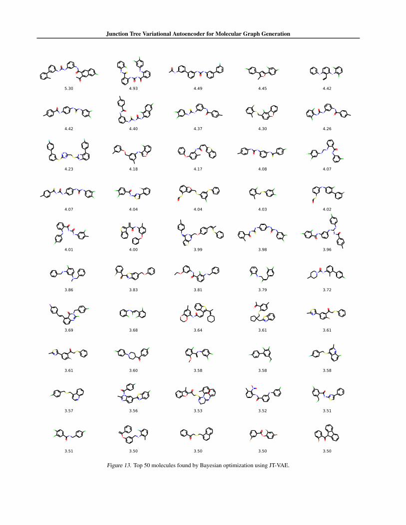
Junction Tree Variational Autoencoder for Molecular Graph Generation

O

ClO

NH

NH

O

NH

5.30

O

NH

O

NH

Cl

Cl

NH

SNH

Cl

4.93

O

NH

NH

O

NH

F

4.49

O

Cl

Cl

Cl

4.45

NH NH

Cl

Cl

4.42

O

NH

NH

S

NH

Cl

Cl

4.42

O

NH

NH

S

NH

O

NH

Cl

Cl

4.40

O

NH

NH

S

NH

Cl

Cl

4.37

Br

S

O

Cl

4.30

O

NH

NH

O

NH

Cl

Cl

4.26

F

S

N

NH

S

N

F

NH

N

4.23

ONH

O

Cl

4.18

O

NH

O

S

4.17

NH

O

NH

NH

S

Cl

4.08

O

NH

Cl

NH

NHCl

Cl

4.07

S

NH

O

NH

NH

O

NH

Cl

Cl

4.07

O

NH

N

Br

S

Cl

Cl

4.04

O

S

O

S

Cl

S

4.04

Cl

S

Cl

Cl

4.03

O

S

NH

Br

Cl

4.02

NH

O

NH

O

NH

Cl

Cl

4.01

O

NH

O

S

4.00

O

N

S

NNH

S

3.99

O

NH

S

NHNH

O

NH

Cl

Cl

3.98

O

NH

NH

Cl

NH

NH

O

Cl

Cl

3.96

N

Cl

NH

3.86

Br

Br N

O

S

3.83

O

NH

O

NH

Cl

3.81

Cl

ClCl

NHCl

3.79

NH

O

N

Cl

3.72

O

I

N

Cl

N

Cl

3.69

Cl

Cl

Cl

NH

Cl

3.68

S

O

NH

O

O

3.64

O

S

N

S

3.61

N

Br

O

S

S

3.61

N

Br

O

S

S

3.61

O

Cl

N

Cl

3.60

NH

Cl

Cl

Cl

O

3.58

F

Cl

ClCl

3.58

S

FCl

N

3.58

Cl

S

N

3.57

NN

Cl

SN

O

F

3.56

N

S

O

O

N

N

3.53

NH

O

NH

Cl

N+O

O-

3.52

O

NH

N

S

Cl

Cl

3.51

O

NH

Cl

Cl

Cl

3.51

O NH

F

3.50

O

S

3.50

O

O

Br

Br

Br

3.50

OBr

3.50

Figure 13. Top 50 molecules found by Bayesian optimization using JT-VAE.

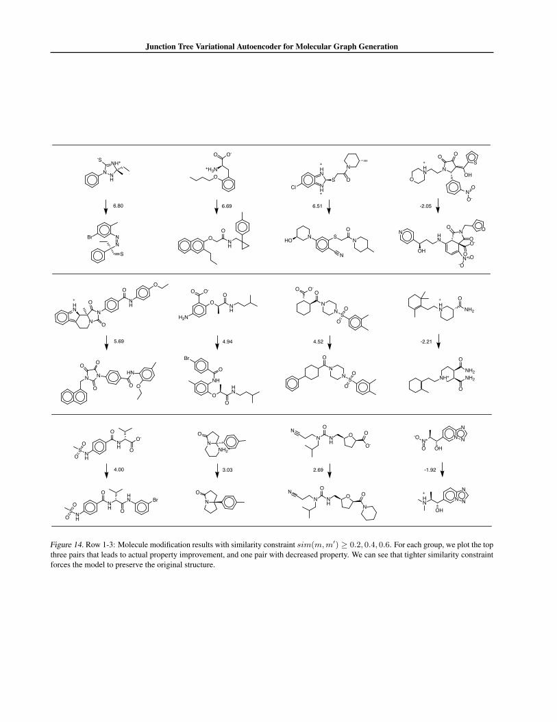
Junction Tree Variational Autoencoder for Molecular Graph Generation

NH

N

-SNH+

S

N

NBr

O

+H3N

O O-

O

O

NH

OO

N

+

HN

O

N+O

O-

OH

S

O

HN

OH

N

N+O

-O

O

O-O

NO

N

OS

+

HN

Cl NH+

N

O

SNHO

N

-2.056.516.696.80

O

NH

O

N

ON

+

HN

O

O

HN

O

N

OO

N

O

NH

O

O

H2N

O O-

O

O

HN

NH

O

Br

S

O

O

N

N

OO O-

S

O

O

N

N

O

+

HN NH2

O

NH+

NH2

O

NH2

O

-2.214.524.945.69

NH

O

NH

S

O

O

O

O-

NH

O

NH

S

O

O

O

HN Br

O

N

NH2+

N

O

N

NO

NH

O

O-

O

N

NO

NH

O

N

O

OH

N

NN

N+

O

-O

OH

N

NN

+

HN

-1.922.693.034.00

Figure 14. Row 1-3: Molecule modification results with similarity constraint sim(m,m′) ≥ 0.2, 0.4, 0.6. For each group, we plot the topthree pairs that leads to actual property improvement, and one pair with decreased property. We can see that tighter similarity constraintforces the model to preserve the original structure.