k-space propagation models for acoustically heterogeneous

k-space propagation models for acoustically heterogeneousmedia: Application to biomedical photoacoustics

B. T. Coxa� and S. KaraDepartment of Medical Physics and Bioengineering, University College London, Gower Street, LondonWC1E 6BT, United Kingdom

S. R. ArridgeDepartment of Computer Science, University College London, Gower Street, London WC1E 6BT, UnitedKingdom

P. C. BeardDepartment of Medical Physics and Bioengineering, University College London, Gower Street, LondonWC1E 6BT, United Kingdom

�Received 29 September 2006; revised 22 February 2007; accepted 22 February 2007�

Biomedical applications of photoacoustics, in particular photoacoustic tomography, require efficientmodels of photoacoustic propagation that can incorporate realistic properties of soft tissue, such asacoustic inhomogeneities both for purposes of simulation and for use in model-based imagereconstruction methods. k-space methods are well suited to modeling high-frequency acousticsapplications as they require fewer mesh points per wavelength than conventional finite element andfinite difference models, and larger time steps can be taken without a loss of stability or accuracy.They are also straighforward to encode numerically, making them appealing as a general tool. Therationale behind k-space methods and the k-space approach to the numerical modeling ofphotoacoustic waves in fluids are covered in this paper. Three existing k-space models are appliedto photoacoustics and demonstrated with examples: an exact model for homogeneous media, asecond-order model that can take into account heterogeneous media, and a first-order model that canincorporate absorbing boundary conditions.© 2007 Acoustical Society of America. �DOI: 10.1121/1.2717409�

PACS number�s�: 43.35.Ud, 43.20.Px �TDM� Pages: 3453–3464

I. INTRODUCTION

The photoacoustic �PA� effect, in which the absorptionof light leads to the generation of an acoustic wave via thethermoelastic expansion of the absorbing region, has foundapplication in many fields,1 some of the most important be-ing spectroscopy,2,3 microscopy,4–6 and biomedicine.7 Bio-medical photoacoustic tomography �PAT�, in particular, hasreceived increasing attention in recent years.8,9 Both clinicaland life sciences applications have been proposed, includingimaging of the breast,10 vasculature,11 and small animals.12,13

As soft tissue is usually highly optically scattering, imagingto high resolution using purely optical means is difficult.However, for acoustic waves, even up to tens of megahertz,the scattering is considerably lower. PAT can therefore com-bine the good resolution of ultrasound ��100 �m� with thehigh contrast and spectroscopic advantages offered by im-ages related to optical absorption.

Most PAT reconstruction algorithms assume that boththe sound speed and density in the sample are uniform.7,14–22

which is not true of soft tissue in general, particularly at highfrequencies. The extent to which the naturally occurringacoustic heterogeneities distort the PAT images remainslargely an open question. One way to answer such questions

a�
Electronic mail: [email protected]
J. Acoust. Soc. Am. 121 �6�, June 2007 0001-4966/2007/121�6

without undertaking extensive experimental studies is tosimulate the experimental measurements using a numericalforward model, so that the effect of heterogeneities on imageresolution and artifact generation can be studied systemati-cally. A further application of a photoacoustic forward modelis in model-based image reconstruction algorithms forPAT.23,24 Model-based image reconstructions make no as-sumptions of acoustic homogeneity, and form an image byiteratively updating a forward model. For iterative recon-struction algorithms such as this to be practical, it is impera-tive that the forward model is computationally efficient.

A numerical, time domain, model based on Poisson’ssolution to the wave equation has been widely used for cal-culating the pressure time history at a point from a photoa-coustically generated source in homogeneous media.25,26

This model has also been adapted to accommodate smallsound speed heterogeneities.23 More recently, finitedifference27 and �frequency domain� finite elementmethods28 have been presented as techniques for modelingphotoacoustics in heterogeneous media. This paper is con-cerned with wave number domain or k-space methods, whichcan achieve the same accuracy as the above-mentioned meth-ods despite using a much coarser spatial grid, and can takemuch larger time steps without causing instabilities. k-spacemethods are therefore computationally efficient, and areideal as forward models in model-based image reconstruc-
tion algorithms for PAT. In addition to being efficient and
© 2007 Acoustical Society of America 3453�/3453/12/$23.00

accurate, numerical k-space models in both two and threedimensions are straightforward to encode. In view of theseadvantages, it is surprising that k-space methods are notmore widely used for studying photoacoustic propagation. Todate, photoacoustic propagation has been calculated usingk-space methods only for homogeneous media.29–31 Here wereview two further k-space models,32,33 originally derived todescribe ultrasonic scattering due to heterogeneous media,and by adding a photoacoustic source term to each, demon-strate their use in photoacoustics with several examples.

II. FORWARD MODELS IN PHOTOACOUSTICS

A. Photoacoustic wave equation

The forward or direct problem in photoacoustics is topredict the acoustic field as a function of time following theabsorption of an optical pulse. If a region of a fluid is heatedby the absorption of a pulse of light, then a sound wave isgenerated. In a stationary fluid, under conditions whereby thesound generation mechanism is thermoelastic and terms con-taining the viscosity and thermal conductivity arenegligible—a regime called thermal confinement—theacoustic pressure, p�x , t�, in the linear acoustic approxima-tion and in the absence of absorption, obeys

�2p

�t2 − c2� � · �1

�� p� = �

�H�t

, �1�

where the sound speed c�x� and density ��x� vary with po-sition x. � is a dimensionless constant called the Grüneisenparameter, which indicates the efficiency of conversion ofabsorbed optical energy �heat� to pressure, and is defined as�=c2� /Cp, where � is the volume thermal expansivity andCp is the specific heat capacity. H�x , t� is the heat energy perunit volume and per unit time deposited in the fluid and, likethe pressure p, will depend, in general, on both position xand time t. When the sound speed and density are uniform,so c�x�=c0 and ��x�=�0, then Eq. �1� becomes

��2/�t2 − c02�2�p = � � H/�t . �2�

If the photoacoustic source term H�x , t� is stationary, then itmay be separated into spatial and temporal componentsH�x , t�=Hx�x�Ht�t�, where Hx�x� is the heat deposited in thefluid per unit volume, and Ht�t� describes the temporal shapeof the pulse, normalized so that the integral of Ht is unity.For instance, if the heating pulse is assumed Gaussian then

Ht�t� =e−�t/��2

��. �3�

As �→0 this pulse Ht�t�→��t� so if c� is much shorter thana typical distance across the heated region, a regime knownas “stress confinement,” then the PA source term may beconsidered to be instantaneous and well-represented by thetime-derivative of a � function. In this case, the forwardproblem reduces to the initial value problem �IVP� for thehomogeneous wave equation

��2/�t2 − c02�2�p = 0 �4�

with initial conditions

3454 J. Acoust. Soc. Am., Vol. 121, No. 6, June 2007

p�t=0 = �Hx, � p/�t�t=0 = 0. �5�

In the examples below we assume x�R2, as it is morestraightforward to display images of a two-dimensional �2D�wave field, but all the algorithms may be easily extended tothree spatial dimensions.

B. Models based on Poisson’s solution

Under conditions of thermal confinement, i.e., instanta-neous heating, Poisson’s solution to the IVP in Eqs. �4� and�5� may be used to calculate the acoustic field

p�x,t� =�

4�c0

�

�t

A�t�

Hx�x��R

dA , �6�

where R= �x−x��, and A�t� is the surface on which R=c0t andis thus a function of time. The optical excitation pulse istaken to occur at t=0. This equation has been implementednumerically by a number of authors25,26 by defining Hx�x� /Ron a mesh and summing the contributions that lie within thetwo circles A�t� and A�t+t� for t=0, t , . . . . The resultingtime series is numerically differentiated to give the acousticpressure. This model was extended to take into account thespatial averaging effect of a finite-sized detector by Köstliand Beard,34 by convolving the detector volume D�x� withHx�x� prior to carrying out the integration over A. Xu andWang23 investigated the effects of sound speed heterogene-ities on breast thermoacoustic tomography by developinganalytical expressions for the effect on the amplitude anddelay of a pulse. They concluded that the effect of a timedelay is more important in imaging, and so adapted Pois-son’s model to incorporate a first-order correction for differ-ent times-of-flight through the heterogeneous medium, bywarping the surface A.

The advantage of this model is that it is intuitive, andcan be an aid to visualizing the forward problem. It is, how-ever, computationally inefficient, and limited in the degree towhich it can model boundaries or heterogeneous acousticproperties. For more complex situations, one approach is toturn to two well-established tools of numerical modeling:finite element and finite difference methods.

C. Finite element and finite difference methods

The finite element �FE� method is a popular and power-ful method for calculating numerical solutions to partial dif-ferential equations because of its flexibility, accuracy, andrigorous mathematical foundations. In this method, the solu-tion is represented by a linear combination of N-dimensionalbasis functions defined on the computational domain, and theunknown amplitudes of these functions are calculated to givea solution, exact at N nodes and approximate in between.The flexibility in the choice of basis functions allows do-mains and heterogeneities of any shape to be well-approximated, and, more important, the basis functions canbe chosen to have support over only a small part of thedomain, so calculation of the unknown amplitudes can bereduced to a sparse matrix equation for which there are effi-cient solvers available. Heterogeneous material properties
can be straightforwardly included, and the well-developed
Cox et al.: k-space models in photoacoustics

mathematical fundamentals of the technique allow thoroughanalyses of errors and sensitivities. Encoding the FE method,however, is not as straightforward as the finite difference�FD� or k-space methods discussed in the following, al-though many commercial packages are now available to easethis burden. Another disadvantage is that, when solving waveproblems with the FE method, about 10 nodes per wave-length are required to represent the field accurately, so high-frequency, large-scale, applications soon become intractable.Jiang et al.28 have used the FE method to find low frequencysolutions of a PA Helmholtz-like equation which includesterms for sound speed heterogeneity and acoustic absorption.

Another group of techniques that is in widespread usefor finding numerical solutions to partial differential equa-tions is that of finite differences, in which derivatives in thepartial differential equation are approximated by differences,thus converting the PDE into a difference equation whichcan be solved numerically. FD models are less flexible thanFE models because, usually, a regular computational meshmust be used. The high-frequency sampling requirement,which is disadvantageous to FE methods, is a problem heretoo. Nevertheless, the popularity of FD methods endures,perhaps because of their conceptual simplicity. Huang et al.27

describe a FD time-domain simulation of PA propagation,which includes nonlinear terms and dissipative effects, and istherefore more general than any of the other models de-scribed in this paper, although the underlying equations arecorrespondingly more complex. For biomedical applications,the assumptions of linearity and thermal confinement—which are required for all the models in this paper—seem tobe valid, and allow considerable simplification of the gov-erning equations, and therefore of the model.

For time domain problems, it is common practice to usea FD approximation to the time derivative, whether the spa-tial part of the solution is solved using FD or FE methods.Approximating the time derivative in this way can introducenumerical dispersion, in which the speed of the wave de-pends, erroneously, on its frequency, thus distorting theshape of pulses. To avoid this, small time steps must betaken, further reducing the efficiency of both FE and FD timedomain models.

D. Pseudospectral and k-space models

The FE and FD methods, although excellent for manyapplications, become cumbersome and slow when modelinglarge scale, high-frequency acoustics applications, due to therequirements for many mesh points for wavelength, andsmall time steps required to minimize unwanted dispersion.In this section we briefly describe the pseudospectral �PS�method, which can help reduce the first of these problems,and k-space propagators, to overcome the second.

In a simple FD scheme, the gradient of the field is esti-mated by fitting a straight line between its values at twomesh points. A better estimate of the gradient could be ob-tained by fitting a higher-order polynomial to a greater num-ber of points, and calculating the derivative of the polyno-mial. The more points used, the higher the degree of
polynomial required, and the more accurate the estimate of

the derivative. The PS method takes this idea further and fitsa Fourier series to all the data on each line of the mesh. Thischoice of interpolating function assumes that the solution isperiodic �the values and the derivatives at both ends of eachline of the mesh are the same� which will rarely be the case.The “wrapping” effects of this assumption are common to PSand k-space methods and are seen in the example in Sec. IVA. Such effects can often be ameliorated using absorbingboundary conditions �see Sec. V and references therein�.There are two significant advantages to using Fourier series.The first is that the amplitudes of the Fourier componentscan be calculated efficiently using the Fast Fourier transform�FFT�, and the gradient calculated simply asF−1ikxFp�x��, where F·� is a Fourier transform andF−1·� its inverse. The second advantage is that the basisfunctions assumed by the FT are sinusoidal, so only twonodes per wavelength are required in order to describe awave, rather than 10+ in the FE and FD methods.

Now, both PS time-domain �PSTD� and k-space meth-ods calculate the spatial gradients using FFTs, as just de-scribed. However, whereas the PSTD method approximatesthe temporal gradient with a finite difference, in k-spacemethods the field is propagated forward in time according toa k-space propagator, which is exact for homogeneous me-dia, and, for heterogeneous media, allows much larger timesteps for similar accuracy and stability to FDmethods.32,33,35–39 In Ref. 39 the k-space method is shown togive more accurate results than a second-order FD methodfor elastic wave propagation even when the time step islarger. References 32 and 33 describe benchmark studies ofthe accuracy of the k-space method in comparison with aleapfrog PSTD method and a time domain FD method. Ex-amples of propagation through samples realistic of soft tissuewere calculated using each model for a range of values of theCourant-Friedrichs-Lewy number, CFL�c0t /x, and it isshown that the error norm increases much more slowly withCFL for the k-space method than for either of the other twomethods. It was also shown that the number of mesh pointsper wavelength required for a given accuracy is much less� 3 as opposed to 10� for the k-space method than for theFD method.

As well as being efficient by virtue of the reduced point-per-wavelength requirement, the use of the FFT to calculatethe gradients in k space, and larger time steps made possibleby the k-space time propagator, another attraction of k-spacemodels is that they are straightforward to encode. In thispaper, three efficient, k-space forward models of photoacous-tic wave generation and propagation are described. All threecalculate the acoustic field as a function of time, given anarbitrary distribution of absorbed optical energy. This firstmodel applies only to homogeneous media,29 whereas thesecond32 and third33 include the effects of acoustic heteroge-neities, i.e., spatial variations in the sound speed and density.The differences between the second and third are that thelatter can incorporate absorbing boundary conditions and
bulk acoustic absorption.

III. k-SPACE MODEL FOR A HOMOGENEOUSMEDIUM

When the sound speed and density are constant every-where, then the photoacoustic waves propagate according toEq. �2�. Following spatial Fourier transformation, Eq. �2�becomes an ODE in time, describing the motion of planewaves with wave vector k= �kx ,ky�,

� d2

dt2 + �c0k�2�p = S�t� , �7�

where the caret indicates a function in k space, and k is the

modulus of k. The source term S�t� is given by

S�t� = �Hx�Ht

�t. �8�

The Green’s function solution to Eq. �7� is

p�k,t� = 0

t

g�t − t��S�t��dt� �9�

=�Hx g�t − t��dHt

dt��t��dt�, �10�

where the Green’s function g is a solution to d2g /dt2

+ �c0k�2g=��t� and is given by

g�k,t� = �0, t � 0

sin�c0kt�/�c0k� , t 0.�11�

When Ht�t�=��t�, an instantaneous pulse at t=0, the solutionfor the pressure becomes

p�k,t� = �Hx � sin�c0k�t − t��c0k

��t��dt�

= �Hx cos�c0kt� �12�

so the acoustic field at time t following an optical pulse att=0 can be calculated using

p�x,t� = �F−1Hx�k�cos�c0kt�� . �13�

This is an exact solution, so the acoustic field can be calcu-lated directly for any time t without having to step throughthe previous times from t=0. In this sense, the cos�ckt� termin Eq. �13� can be considered as an exact time propagator.�To calculate pressure time histories on just a single planeperpendicular to the axis of symmetry in a radially sym-metric field, the vertical wave-number-frequency mappingtechnique described in Cox and Beard29 is considerablymore efficient.�

It is instructive to see that the solution in Eq. �13� can bewritten as an explicitly time-stepping, finite-difference-stylesolution, in which the field at t+t is calculated from thefield at times t and t−t. Consider the transformed field,ˆ
p�k�, at the two times t+t and t−t:

p�t + t� = �Hx cos�c0k�t + t��

= �Hx�cos�c0kt�cos�c0kt�

− sin�c0kt�sin�c0kt�� , �14�

p�t − t� = �Hx cos�c0k�t − t��

= �Hx�cos�c0kt�cos�c0kt�

+ sin�c0kt�sin�c0kt�� . �15�

So,

p�t + t� + p�t − t� = 2�Hx cos�c0kt�cos�c0kt�

= 2p�t�cos�c0kt�

= 2p�t��1 − 2 sin2�c0kt/2�� 16�

and rearranging gives

p�t + t� − 2p�t� + p�t − t� = − 4 sin2�c0kt/2�p�t� .

�17�

This is a time-stepping solution for which steps t of anysize may be used without introducing error. This is an exactrearrangement of Eq. �13�, so by using the initial conditions

p�−t�=�Hx cos�c0kt� and p�0�=�Hx, exactly the samesolutions for any t�0 will be calculated. By comparingEq. �17� to a pseudospectral, leapfrog FD scheme, basedon Eq. �7� in the absence of the source term,

p�t + t� − 2p�t� + p�t − t�t2 = − �c0k�2p�t� �18�

we can see that the 4 sin2�c0kt /2� term in Eq. �17� hasreplaced the term �c0kt�2 in Eq. �18�. For small timesteps these are equal, but for larger time steps the latterleads to numerical dispersion whereas the former providesan exact, dispersion-free, solution. Of course, with�-function heating, there is no need for such a time step-ping scheme as we have an exact propagator for arbitrarilylarge time steps, Eq. �13�. Indeed, the solution for a finite-duration Gaussian excitation pulse could be obtained bymultiplying the Fourier transform of Eq. �3� to the otherk-space terms in Eq. �13�. However, when considering asource with an arbitrary temporal pulse shape, or propa-gation through heterogeneous media, a time-steppingscheme may be required. We can extend the time-steppingscheme in Eq. �17� to include a source with an arbitrarypulse shape:

p�t + t� − 2p�t� + p�t − t� = − 4 sin2�c0kt/2��p�t�

−S�t�

2� . �19�
�c0k�

A. Example: Laser beam incident on an absorbinghalf-space

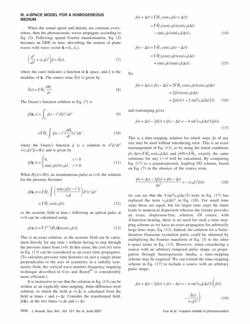
A two-dimensional �2D� example of a tophat laser beamincident on a pure �nonscattering� absorber is used to dem-onstrate the homogeneous model in Eq. �19�. Figure 1 showsthe arrangement: A collimated laser beam with a6 mm diameter tophat profile, indicated by an arrow, is inci-dent on an optically absorbing half-space, the surface ofwhich is marked by a dotted line. The optical absorptioncoefficient �a=5 mm−1. The absorbed optical energy resultsin a spatially varying heating function, Hx�x�, which decaysexponentially from the boundary according to the Beer-Lambert law, and is shown in Figs. 1 and 2 �top left� as adark region. As this example has 2D symmetry, with novariation into or out of the plane of the paper, the tophatbeam effectively models a three-dimensional �3D� linesource. The laser fluence at the surface of the absorber wasset to 10 mJ/cm2 �i.e., 10 mJ/cm per cm into the plane ofthe paper�. The sound speed and density were 1500 m/s and1000 kg/m3, respectively, and the Grüneisen parameter �=0.11, their values in water �the major constituent of softtissue�. The 2D computational grid of 10 mm�10 mm, was

FIG. 1. A collimated laser beam with a 6-mm-diam tophat profile, indicatedwith an arrow, is incident on an optically absorbing half-space, the surfaceof which is marked by a dotted line. The optical absorption coefficient �a

=5 mm−1. The absorbed energy distribution decays exponentially from theboundary according to the Beer-Lambert law. The laser fluence at the sur-face was 10 mJ/cm2 �i.e., 10 mJ/cm per cm into the plane of the paper�.The sound speed and density were 1500 m/s and 1000 kg/m3, respectively,and the Grüneisen parameter �=0.11. The evolution of this acoustic field isshown in Fig. 2.

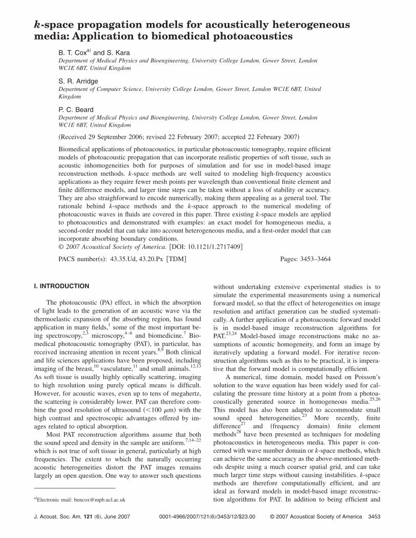
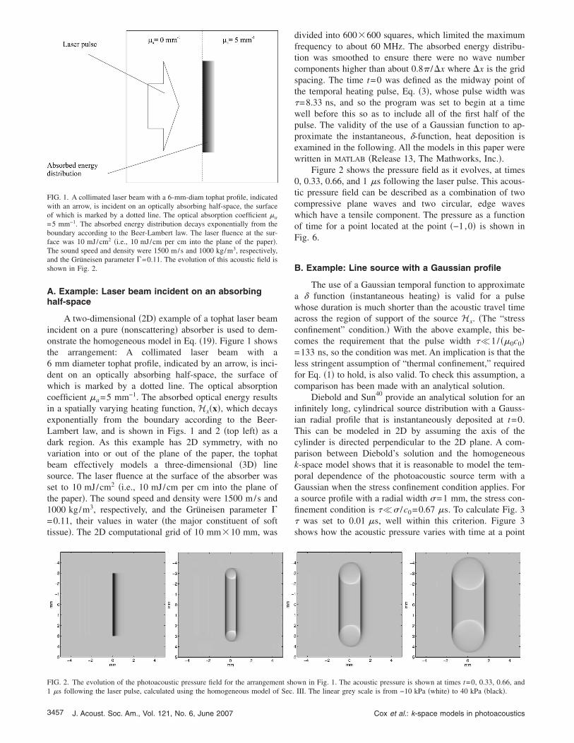
FIG. 2. The evolution of the photoacoustic pressure field for the arrangeme
1 �s following the laser pulse, calculated using the homogeneous model of Sec.

divided into 600�600 squares, which limited the maximumfrequency to about 60 MHz. The absorbed energy distribu-tion was smoothed to ensure there were no wave numbercomponents higher than about 0.8� /x where x is the gridspacing. The time t=0 was defined as the midway point ofthe temporal heating pulse, Eq. �3�, whose pulse width was�=8.33 ns, and so the program was set to begin at a timewell before this so as to include all of the first half of thepulse. The validity of the use of a Gaussian function to ap-proximate the instantaneous, �-function, heat deposition isexamined in the following. All the models in this paper werewritten in MATLAB �Release 13, The Mathworks, Inc.�.

Figure 2 shows the pressure field as it evolves, at times0, 0.33, 0.66, and 1 �s following the laser pulse. This acous-tic pressure field can be described as a combination of twocompressive plane waves and two circular, edge waveswhich have a tensile component. The pressure as a functionof time for a point located at the point �−1,0� is shown inFig. 6.

B. Example: Line source with a Gaussian profile

The use of a Gaussian temporal function to approximatea � function �instantaneous heating� is valid for a pulsewhose duration is much shorter than the acoustic travel timeacross the region of support of the source Hx. �The “stressconfinement” condition.� With the above example, this be-comes the requirement that the pulse width ��1/ ��0c0�=133 ns, so the condition was met. An implication is that theless stringent assumption of “thermal confinement,” requiredfor Eq. �1� to hold, is also valid. To check this assumption, acomparison has been made with an analytical solution.

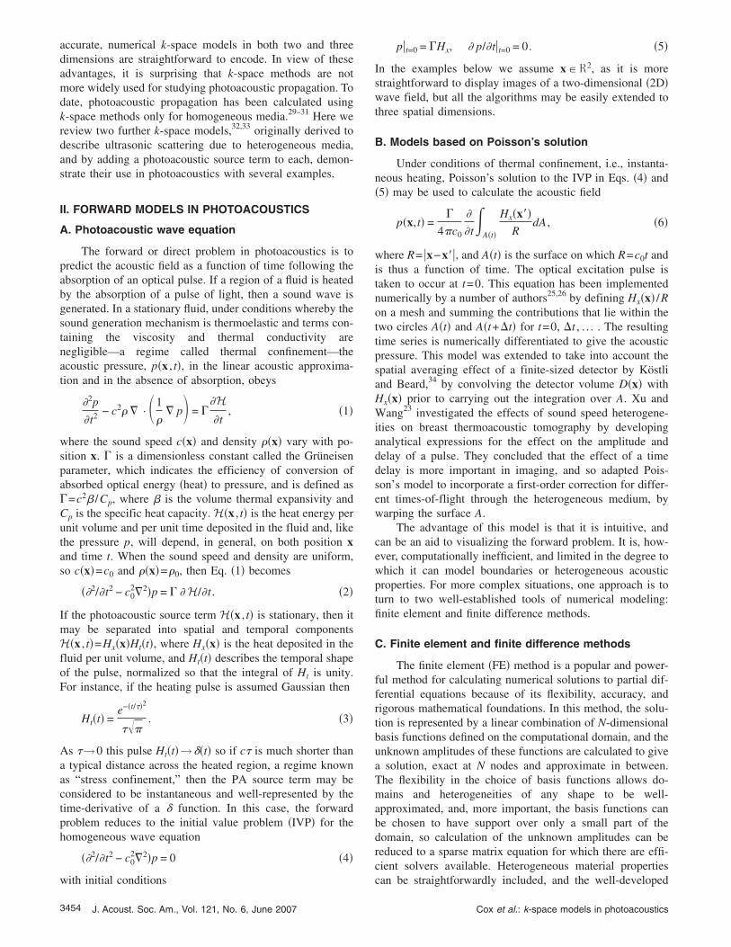
Diebold and Sun40 provide an analytical solution for aninfinitely long, cylindrical source distribution with a Gauss-ian radial profile that is instantaneously deposited at t=0.This can be modeled in 2D by assuming the axis of thecylinder is directed perpendicular to the 2D plane. A com-parison between Diebold’s solution and the homogeneousk-space model shows that it is reasonable to model the tem-poral dependence of the photoacoustic source term with aGaussian when the stress confinement condition applies. Fora source profile with a radial width =1 mm, the stress con-finement condition is �� /c0=0.67 �s. To calculate Fig. 3� was set to 0.01 �s, well within this criterion. Figure 3shows how the acoustic pressure varies with time at a point

wn in Fig. 1. The acoustic pressure is shown at times t=0, 0.33, 0.66, and
nt sho III. The linear grey scale is from −10 kPa �white� to 40 kPa �black�.

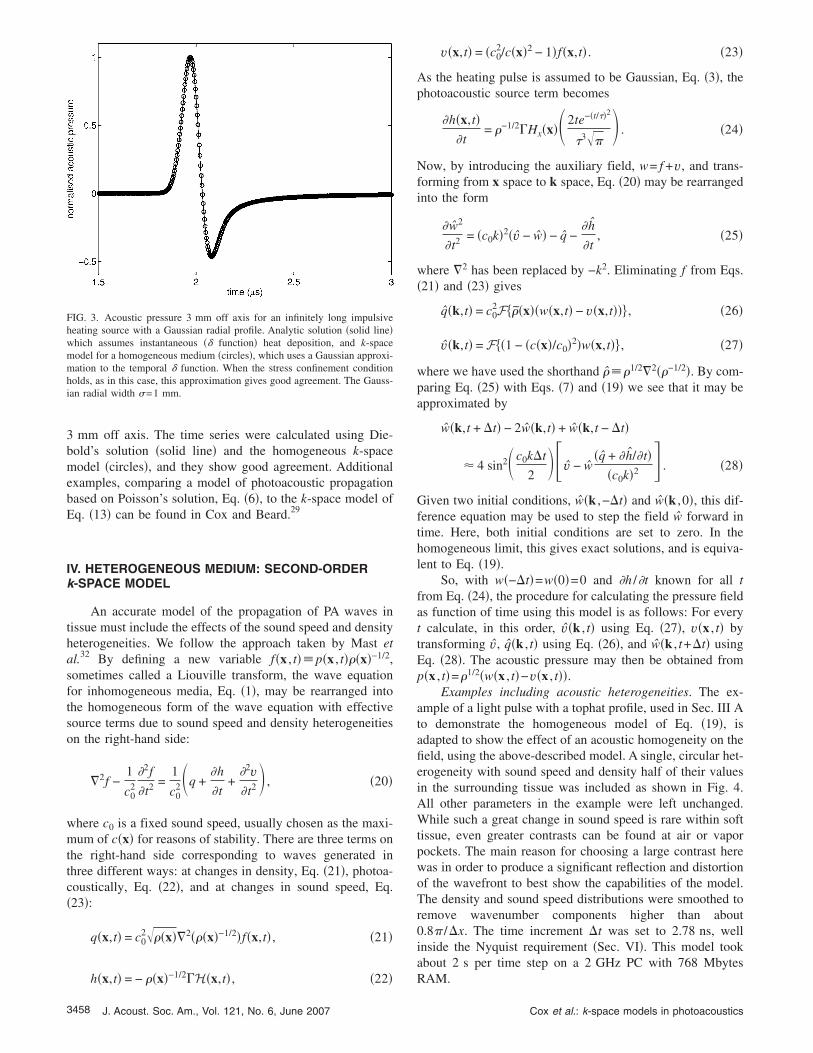
3 mm off axis. The time series were calculated using Die-bold’s solution �solid line� and the homogeneous k-spacemodel �circles�, and they show good agreement. Additionalexamples, comparing a model of photoacoustic propagationbased on Poisson’s solution, Eq. �6�, to the k-space model ofEq. �13� can be found in Cox and Beard.29

IV. HETEROGENEOUS MEDIUM: SECOND-ORDERk-SPACE MODEL

An accurate model of the propagation of PA waves intissue must include the effects of the sound speed and densityheterogeneities. We follow the approach taken by Mast etal.32 By defining a new variable f�x , t�� p�x , t��x�−1/2,sometimes called a Liouville transform, the wave equationfor inhomogeneous media, Eq. �1�, may be rearranged intothe homogeneous form of the wave equation with effectivesource terms due to sound speed and density heterogeneitieson the right-hand side:

�2f −1

c02

�2f

�t2 =1

c02�q +

�h

�t+

�2v�t2 � , �20�

where c0 is a fixed sound speed, usually chosen as the maxi-mum of c�x� for reasons of stability. There are three terms onthe right-hand side corresponding to waves generated inthree different ways: at changes in density, Eq. �21�, photoa-coustically, Eq. �22�, and at changes in sound speed, Eq.�23�:

q�x,t� = c02��x��2��x�−1/2�f�x,t� , �21�

−1/2

FIG. 3. Acoustic pressure 3 mm off axis for an infinitely long impulsiveheating source with a Gaussian radial profile. Analytic solution �solid line�which assumes instantaneous �� function� heat deposition, and k-spacemodel for a homogeneous medium �circles�, which uses a Gaussian approxi-mation to the temporal � function. When the stress confinement conditionholds, as in this case, this approximation gives good agreement. The Gauss-ian radial width =1 mm.

h�x,t� = − ��x� �H�x,t� , �22�


v�x,t� = �c02/c�x�2 − 1�f�x,t� . �23�

As the heating pulse is assumed to be Gaussian, Eq. �3�, thephotoacoustic source term becomes

�h�x,t��t

= �−1/2�Hx�x��2te−�t/��2

�3�� . �24�

Now, by introducing the auxiliary field, w= f +v, and trans-forming from x space to k space, Eq. �20� may be rearrangedinto the form

�w2

�t2 = �c0k�2�v − w� − q −� h

�t, �25�

where �2 has been replaced by −k2. Eliminating f from Eqs.�21� and �23� gives

q�k,t� = c02F��x��w�x,t� − v�x,t�� , �26�

v�k,t� = F�1 − �c�x�/c0�2�w�x,t�� , �27�

where we have used the shorthand ��1/2�2��−1/2�. By com-paring Eq. �25� with Eqs. �7� and �19� we see that it may beapproximated by

w�k,t + t� − 2w�k,t� + w�k,t − t�

4 sin2� c0kt

2��v − w

�q + � h/�t��c0k�2 � . �28�

Given two initial conditions, w�k ,−t� and w�k ,0�, this dif-ference equation may be used to step the field w forward intime. Here, both initial conditions are set to zero. In thehomogeneous limit, this gives exact solutions, and is equiva-lent to Eq. �19�.

So, with w�−t�=w�0�=0 and �h /�t known for all tfrom Eq. �24�, the procedure for calculating the pressure fieldas function of time using this model is as follows: For everyt calculate, in this order, v�k , t� using Eq. �27�, v�x , t� bytransforming v, q�k , t� using Eq. �26�, and w�k , t+t� usingEq. �28�. The acoustic pressure may then be obtained fromp�x , t�=�1/2�w�x , t�−v�x , t��.

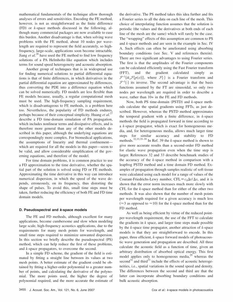
Examples including acoustic heterogeneities. The ex-ample of a light pulse with a tophat profile, used in Sec. III Ato demonstrate the homogeneous model of Eq. �19�, isadapted to show the effect of an acoustic homogeneity on thefield, using the above-described model. A single, circular het-erogeneity with sound speed and density half of their valuesin the surrounding tissue was included as shown in Fig. 4.All other parameters in the example were left unchanged.While such a great change in sound speed is rare within softtissue, even greater contrasts can be found at air or vaporpockets. The main reason for choosing a large contrast herewas in order to produce a significant reflection and distortionof the wavefront to best show the capabilities of the model.The density and sound speed distributions were smoothed toremove wavenumber components higher than about0.8� /x. The time increment t was set to 2.78 ns, wellinside the Nyquist requirement �Sec. VI�. This model tookabout 2 s per time step on a 2 GHz PC with 768 Mbytes
RAM.

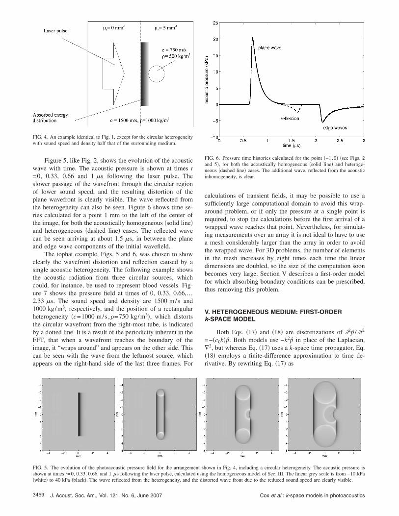
Figure 5, like Fig. 2, shows the evolution of the acousticwave with time. The acoustic pressure is shown at times t=0, 0.33, 0.66 and 1 �s following the laser pulse. Theslower passage of the wavefront through the circular regionof lower sound speed, and the resulting distortion of theplane wavefront is clearly visible. The wave reflected fromthe heterogeneity can also be seen. Figure 6 shows time se-ries calculated for a point 1 mm to the left of the center ofthe image, for both the acoustically homogeneous �solid line�and heterogeneous �dashed line� cases. The reflected wavecan be seen arriving at about 1.5 �s, in between the planeand edge wave components of the initial wavefield.

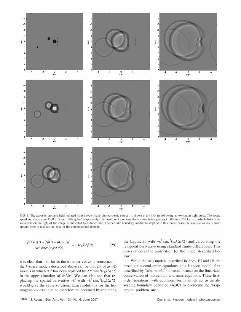
The tophat example, Figs. 5 and 6, was chosen to showclearly the wavefront distortion and reflection caused by asingle acoustic heterogeneity. The following example showsthe acoustic radiation from three circular sources, whichcould, for instance, be used to represent blood vessels. Fig-ure 7 shows the pressure field at times of 0, 0.33, 0.66,…2.33 �s. The sound speed and density are 1500 m/s and1000 kg/m3, respectively, and the position of a rectangularheterogeneity �c=1000 m/s ,�=750 kg/m3�, which distortsthe circular wavefront from the right-most tube, is indicatedby a dotted line. It is a result of the periodicity inherent in theFFT, that when a wavefront reaches the boundary of theimage, it “wraps around” and appears on the other side. Thiscan be seen with the wave from the leftmost source, whichappears on the right-hand side of the last three frames. For

FIG. 4. An example identical to Fig. 1, except for the circular heterogeneitywith sound speed and density half that of the surrounding medium.

FIG. 5. The evolution of the photoacoustic pressure field for the arrangemshown at times t=0, 0.33, 0.66, and 1 �s following the laser pulse, calculated
�white� to 40 kPa �black�. The wave reflected from the heterogeneity, and the dis

calculations of transient fields, it may be possible to use asufficiently large computational domain to avoid this wrap-around problem, or if only the pressure at a single point isrequired, to stop the calculations before the first arrival of awrapped wave reaches that point. Nevertheless, for simulat-ing measurements over an array it is not ideal to have to usea mesh considerably larger than the array in order to avoidthe wrapped wave. For 3D problems, the number of elementsin the mesh increases by eight times each time the lineardimensions are doubled, so the size of the computation soonbecomes very large. Section V describes a first-order modelfor which absorbing boundary conditions can be prescribed,thus removing this problem.

V. HETEROGENEOUS MEDIUM: FIRST-ORDERk-SPACE MODEL

Both Eqs. �17� and �18� are discretizations of �2p /�t2

=−�c0k�p. Both models use −k2p in place of the Laplacian,�2, but whereas Eq. �17� uses a k-space time propagator, Eq.�18� employs a finite-difference approximation to time de-rivative. By rewriting Eq. �17� as

own in Fig. 4, including a circular heterogeneity. The acoustic pressure isg the homogeneous model of Sec. III. The linear grey scale is from −10 kPa

FIG. 6. Pressure time histories calculated for the point �−1,0� �see Figs. 2and 5�, for both the acoustically homogeneous �solid line� and heteroge-neous �dashed line� cases. The additional wave, reflected from the acousticinhomogeneity, is clear.

ent shusin

torted wave front due to the reduced sound speed are clearly visible.


p�t + t� − 2p�t� + p�t − t�t2 sinc2�c0kt/2�

= − �c0k�2p�t� �29�

it is clear that—so far as the time derivative is concerned—the k-space models described above can be thought of as FDmodels in which t2 has been replaced by t2 sinc2�c0kt /2�in the approximation of �2 /�t2. We can also see that re-placing the spatial derivative −k2 with −k2 sinc2�c0kt /2�would give the same solution. Exact solutions for the ho-

FIG. 7. The acoustic pressure field radiated from three circular photoacoustspeed and density are 1500 m/s and 1000 kg/m3, respectively. The position owavefront on the right of the image, is indicated by a dotted line. The perioaround when it reaches the edge of the computational domain.

mogeneous case can be therefore be obtained by replacing


the Laplacian with −k2 sinc2�c0kt /2� and calculating thetemporal derivative using standard finite-differences. Thisobservation is the motivation for the model described be-low.

While the two models described in Secs. III and IV arebased on second-order equations, this k-space model, firstdescribed by Tabei et al.,33 is based instead on the linearizedconservation of momentum and mass equations. These first-order equations, with additional terms which act as an ab-sorbing boundary condition �ABC� to overcome the wrap-

rces is shown every 1/3 �s following an excitation light pulse. The soundctangular acoustic heterogeneity �1000 m/s, 750 kg/m3�, which distorts the

oundary conditions implicit in this model cause the acoustic waves to wrap

ic souf a re

dic b

around problem, are


�u

�t= −

�p

�− � · u , �30�

�p

�t= − �c2 � · u + �H − ��x + �y�p , �31�

where �H is the PA source term and the two terms contain-ing �= ��x�x� ,�y�x�� represent the ABC. The principle ad-vantage of using two first-order equations is that the vectoru= �ux ,uy� appears explicitly and it is therefore possible tointroduce direction-dependent absorption, which cannot bedone when only the scalar p is available. By defining theabsorption � to be zero everywhere except in a layer close tothe edges of the domain, and in that layer to be zero in alldirections except normal to the boundary, the amplitude ofthe waves leaving the domain �and only those leaving thedomain� can be reduced to virtually nothing, and the wrap-

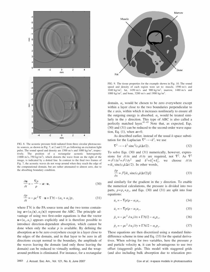
FIG. 8. The acoustic pressure field radiated from three circular photoacous-tic sources, as shown in Fig. 7, at 2 and 2.33 �s following an excitation lightpulse. The sound speed and density are 1500 m/s and 1000 kg/m3, respec-tively. The position of a rectangular acoustic heterogeneity�1000 m/s ,750 kg/m3�, which distorts the wave front on the right of theimage, is indicated by a dotted line. In contrast to the final two frames ofFig. 7, the acoustic waves do not wrap around when they reach the edge ofthe computational domain, but are rather attenuated to almost zero, due tothe absorbing boundary condition.

around problem is eliminated. For instance, for a rectangular


domain, �x would be chosen to be zero everywhere exceptwithin a layer close to the two boundaries perpendicular tothe x axis, within which it increases nonlinearly to ensure allthe outgoing energy is absorbed. �y would be treated simi-larly in the y direction. This type of ABC is also called aperfectly matched layer.41–43 Note that, as expected, Eqs.�30� and �31� can be reduced to the second-order wave equa-tion, Eq. �1�, when �=0.

As described earlier, instead of the usual k-space substi-tution for the Laplacian �2→−k2, we use

�2 → − k2 sinc2�c0kt/2� . �32�

To solve Eqs. �30� and �31� numerically, however, expres-sions for � /�x and � /�y are required, not �2. As �2

��2 /�x2+�2 /�y2 and k2=kx2+ky

2, we choose � /�x= ikx sinc�c0kt /2�. In other words,

�p

�x= Fikx sinc�c0kt/2�p� �33�

and similarly for the gradient in the y direction. To enablethe numerical calculations, the pressure is divided into twoparts, p= px+ py, and Eqs. �30� and �31� are split into fourequations:

ux = − �p/� − �xux, �34�

uy = − �p/� − �yuy , �35�

px = − �c2 � ux/�x + �H/2 − �xpx, �36�

py = − �c2 � uy/�y + �H/2 − �ypy . �37�

These equations are then discretized using a standard finite-difference scheme in time and Eq. �33� for the spatial deriva-tives. When solving for two variables, here the pressure pand particle velocity u, it can be advantageous to use twooffset �staggered� grids. This model with staggered grids

FIG. 9. The tissue properties for the example shown in Fig. 10. The soundspeed and density of each region were set to: muscle, 1590 m/s and1040 kg/m3, fat, 1450 m/s and 900 kg/m3, marrow, 1480 m/s and1000 kg/m3, and bone, 3200 m/s and 1900 kg/m3.

�and also including bulk absorption due to relaxation pro-


the h

cesses� is described in Tabei et al.33 Such an implementationwas used for the following examples.

Examples using the first-order model. The example

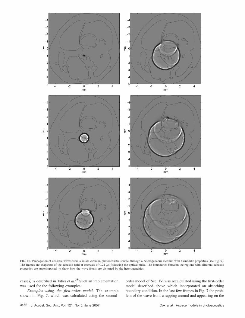
FIG. 10. Propagation of acoustic waves from a small, circular, photoacousticThe frames are snapshots of the acoustic field at intervals of 0.21 �s followproperties are superimposed, to show how the wave fronts are distorted by

shown in Fig. 7, which was calculated using the second-


order model of Sec. IV, was recalculated using the first-ordermodel described above which incorporated an absorbingboundary condition. In the last few frames in Fig. 7 the prob-

ce, through a heterogeneous medium with tissue-like properties �see Fig. 9�.e optical pulse. The boundaries between the regions with different acousticeterogeneities.

souring th

lem of the wave front wrapping around and appearing on the


far side of the image is evident. Figure 8 shows the pressurefield at times corresponding to the last two frames of Fig. 7,but calculated by the first-order model. It is clear that thewrapping problem has been removed.

The final example, shown in Fig. 9, contains a degree ofheterogeneity more representative of tissue. The model canaccount for continuously varying acoustic properties, al-though here the domain is divided into four types of tissuewith different acoustic properties. The sound speeds and den-sities of the four tissue types were set to: muscle, 1590 m/sand 1040 kg/m3, fat, 1450 m/s and 900 kg/m3, marrow,1480 m/s and 1000 kg/m3, and bone, 3200 m/s and1900 kg/m3. A small circular PA source, that could for in-stance represent a blood vessel or a tumor, or a region withhigh chromophore concentration for another reason, isshown in the first frame of Fig. 10. This simple PA sourcewas chosen so that the effect of the inhomogeneities on thewave fronts would be readily observable. It would be quiteas straightforward to define a PA source with a complex ge-ometry. The boundaries between the different tissue typeshave been superimposed on the images. The greyscale hasbeen set the same in each image, which has led to somethresholding of the wave amplitude in the first few images.This allows the reflected and refracted waves to be seen moreclearly. The frames are spaced by 0.21 �s. The most signifi-cant change to the circular wave front is, as expected, fromthe tissue-bone interface, where there is the greatest acousticimpedance change. The reflected wave and the reduced am-plitude of the transmitted wave are visible. The distortingeffect of the differences in the sound speed between themuscle and fat regions of the tissue can also be seen, forexample, on the left-hand side of the wave.

VI. DISCUSSION

PA sources or distributions of acoustic properties thatcontain discontinuities or very large gradients at some pointsrequire high wave numbers in order to describe them accu-rately. In FFT-based, k-space methods, there is a limit to thehighest permissible wave number, a requirement imposed bythe need to prevent aliasing �when a wave number compo-nent is undersampled and appears at a lower wave number�.There must be no components higher than the Nyquist wavenumber, defined as 0.5�2� /x�, where x is the grid spac-ing. It is therefore important, when using k-space methods, tospatially smooth the acoustic properties and the spatial partof the source term in order to ensure there are no componentsat wave numbers above this limit. This could be consideredto be a disadvantage to the k-space approach, becausesmoothed—and therefore approximate—versions of thesound speed, density, and source distributions are used whencalculating the acoustic field. However, the high wave num-ber components, which are removed by smoothing, wouldonly have contributed to the high frequency part of the field,and as, in practice, all measurements are bandlimited by thedetectors or ultrasonic absorption to some extent, only thosewave numbers that contribute to the measured field are re-quired for the model to simulate the acoustic pressure mea-
surements accurately. In other words, when modeling mea-

surements made by a pressure detector with a finitebandwidth, it is not necessary to include components of thefield outside this bandwidth. Indeed, to obtain accurate simu-lations of data measured with a real, nonidealized, detector, awave number model of the angle- and frequency-dependentresponse of a sensor44 can be incorporated into a k-spacemodel simply by multiplication, and without requiring anexplicit convolution.

When calculating acoustic pressure time histories, it isimportant to ensure the time step, t, is sufficiently small toensure the sampling rate is greater than the temporal Nyquistrate �i.e., half the maximum frequency�. With k-space modelsthis requirement is that t is less than the minimum value ofx /c. For the above examples, t was 0.2−0.4x /c.

All the models described in this paper are for photoa-coustically generated waves propagating in fluids. In somecircumstances it will be necessary to include the effect ofshear waves on the propagation. k-space models for elasticwave propagation in solids have also been described,39 andcould be applied in these cases.

VII. SUMMARY

k-space models have been proposed as a straightforwardand computationally efficient approach to modeling the for-ward problem in biomedical photoacoustics, in particular, tosimulating, accurately, time series measured with a bandlim-ited detector. k-space models of photoacoustic waves can besignificantly more efficient than corresponding FE and FDmethods, as k-space methods address the particular difficultyof modeling high-frequency acoustic waves on a large scaleby requiring fewer mesh points per wavelength and allowinglarger time steps without reducing accuracy or introducinginstability. The k-space method of numerical modeling ofphotoacoustic waves in fluids is described, and the rationalebehind three particular k-space models �one for homoge-neous media, one for heterogeneous media, and a model thatcan incorporate absorbing boundary conditions� has been ex-plained. Examples of photoacoustic wave propagation in het-erogenous, tissue-like, media are given.

ACKNOWLEDGMENT

This work has been supported by the Engineering andPhysical Sciences Research Council, UK.

1A. C. Tam, “Applications of photoacoustic sensing techniques,” Rev. Mod.Phys. 58, 381–431 �1986�.

2G. A. West, J. J. Barrett, D. R. Siebert, and K. V. Reddy, “Photoacousticspectroscopy,” Rev. Sci. Instrum. 54, 797–817 �1983�.

3J. G. Laufer, C. Elwell, D. Delpy, and P. Beard, “In vitro measurements ofabsolute blood oxygen saturation using pulsed near-infrared photoacousticspectroscopy: Accuracy and resolution,” Phys. Med. Biol. 50, 4409–4428�2005�.

4A. Rosencwaig, “Photoacoustic microscopy,” Am. Lab. �Shelton, Conn.�11, 39–49 �1979�.

5M. Luukkala and A. Penttinen, “Photoacoustic microscope,” Electron.Lett. 15, 325–326 �1979�.

6H. Zhang, K. Maslov, G. Stoica, and L. Wang, “Functional photoacousticmicroscopy for high-resolution and noninvasive in vivo imaging,” Nat.Biotechnol. 24, 848–851 �2006�.

7M. Xu and L. V. Wang, “Photoacoustic imaging in biomedicine,” Rev. Sci.Instrum. 77, 041101 �2006�.

8
Photons Plus Ultrasound: Imaging and Sensing 2005, edited by A. A.

Oraevsky and L. V. Wang �SPIE, Bellingham, WA, 2005�, Vol. 5697.9Photons Plus Ultrasound: Imaging and Sensing 2006, edited by A. A.Oraevsky and L. V. Wang �SPIE, Bellingham, WA, 2006�, Vol. 6086.

10R. A. Kruger, K. D. Miller, H. E. Reynolds, W. L. Kiser, D. R. Reinecke,and G. A. Kruger, “Contrast enhancement of breast cancer in vivo usingthermoacoustic CT at 434 MHz—feasibility study,” Radiology 216, 279–283 �2000�.

11F. F. M. de Mul and C., G. A. Hoelen, “Three-dimensional imaging ofblood vessels in tissue using photo-acoustics,” J. Vasc. Res. 35, 192–194�1998�.

12X. Wang, Y. Pang, G. Ku, X. Xie, G. Stoica, and L. V. Wang, “Noninva-sive laser-induced photoacoustic tomography for structural and functionalin vivo imaging of the brain,” Nat. Biotechnol. 21, 803–806 �2003�.

13R. Kruger, W. Kiser, D. Reinecke, G. Kruger, and K. Miller, “Thermoa-coustic molecular imaging of small animals,” Mol. Imaging 2, 113–123�2003�.

14S. J. Norton and M. Linzer, “Ultrasonic reflectivity imaging in 3dimensions—Exact inverse scattering solutions for plane, cylindrical, andspherical apertures,” IEEE Trans. Biomed. Eng. 28, 202–220 �1981�.

15R. A. Kruger, P. Liu, Y. R. Fang, and C. R. Appledorn, “Photoacousticultrasound �PAUS�—reconstruction tomography,” Med. Phys. 22, 1605–1609 �1995�.

16P. Y. Liu, “The P-transform and photoacoustic image reconstruction,”Phys. Med. Biol. 43, 667–674 �1998�.

17M. H. Xu, Y. Xu, and L. H. V. Wang, “Time-domain reconstruction-algorithms and numerical simulations for thermoacoustic tomography invarious geometries,” IEEE Trans. Biomed. Eng. 50, 1086–1099 �2003�.

18D. Finch, S. K. Patch, and Rakesh, “Determining a function from its meanvalues over a family of spheres,” SIAM J. Math. Anal. 35, 1213–1240�2003�.

19S. J. Norton and T. Vo-Dinh, “Optoacoustic diffraction tomography:Analysis of algorithms,” J. Opt. Soc. Am. A 20, 1859–1866 �2003�.

20Y. Xu and L. V. Wang, “Time reversal and its application to tomographywith diffracting sources,” Phys. Rev. Lett. 92, 033902 �2004�.

21M. Xu and L. V. Wang, “Universal back-projection algorithm for photoa-coustic computed tomography,” Phys. Rev. E 71, 016706 �2005�.

22J. Zhang, M. A. Anastasio, X. Pan, and L. V. Wang, “Weighted expecta-tion maximization reconstruction algorithms for thermoacoustic tomogra-phy,” IEEE Trans. Med. Imaging 24, 817–820 �2005�.

23Y. Xu and L. Wang, “Effects of acoustic heterogeneity in breast thermoa-coustic tomography,” IEEE Trans. Ultrason. Ferroelectr. Freq. Control 50,1134–1146 �2003�.

24J. Zhang and M. A. Anastasio, “Reconstruction of speed-of-sound andelectromagnetic absorption distributions in photoacoustic tomography,”Proc. SPIE 6086, 608619 �2006�.

25M. Frenz, G. Paltauf, and H. Schmidt Kloiber, “Laser-generated cavitationin absorbing liquid induced by acoustic diffraction,” Phys. Rev. Lett. 76,3546–3549 �1996�.

26G. Paltauf, H. Schmidt Kloiber, and H. Guss, “Light distribution measure-ments in absorbing materials by optical detection of laser-induced stresswaves,” Appl. Phys. Lett. 69, 1526–1528 �1996�.

27
D.-H. Huang, C.-K. Liao, C.-W. Wei, and P.-C. Li, “Simulations of optoa-

coustic wave propagation in light-absorbing media using a finite-differncetime-domain method,” J. Acoust. Soc. Am. 117, 2795–2801 �2005�.

28H. Jiang, Z. Yuan, and X. Gu, “Spatially varying optical and acousticproperty reconstruction using finite-element-based photoacoustic tomogra-phy,” J. Opt. Soc. Am. A 23, 878–888 �2006�.

29B. T. Cox and P. C. Beard, “Fast calculation of pulsed photoacoustic fieldsin fluids using k-space methods,” J. Acoust. Soc. Am. 117, 3616–3627�2005�.

30B. T. Cox, S. Arridge, K. Köstli, and P. Beard, “Quantitative photoacousticimaging: Fitting a model of light transport to the initial pressure distribu-tion,” Proc. SPIE 5697, 49–55 �2005�.

31A. Vogel, J. Noack, G. Hüttman, and G. Paltauf, “Mechanisms of femto-second laser nanosurgery of cells and tissues,” Appl. Phys. B 81, 1015–1047 �2005�.

32T. D. Mast, L. P. Souriau, D.-L. D. Liu, M. Tabei, A. I. Nachman, and R.C. Waag, “A k-space method for large-scale models of wave propagationin tissue,” IEEE Trans. Ultrason. Ferroelectr. Freq. Control 48, 341–354�2001�.

33M. Tabei, T. D. Mast, and R. C. Waag, “A k-space method for coupledfirst-order acoustic propagation equations,” J. Acoust. Soc. Am. 111,53–63 �2002�.

34K. Köstli and P. Beard, “Two-dimensional photoacoustic imaging by useof Fourier-transform image reconstruction and a detector with an aniso-tropic response,” Appl. Opt. 42, 1899–1908 �2003�.

35B. Fornberg and G. B. Whitham, “A numerical and theoretical study ofcertain nonlinear wave phenomena,” Philos. Trans. R. Soc. London, Ser. A289, 373–404 �1978�.

36N. N. Bojarski, “The k-space formulation of the scattering problem in thetime domain,” J. Acoust. Soc. Am. 72, 570–584 �1982�.

37N. N. Bojarski, “The k-space formulation of the scattering problem in thetime domain: An improved single propagator formulation,” J. Acoust. Soc.Am. 77, 826–831 �1985�.

38B. Compani-Tabrizi, “K-space scattering formulation of the absorptive fullfluid elastic scalar wave equation in the time domain,” J. Acoust. Soc. Am.79, 901–905 �1986�.

39Q.-H. Liu, “Generalisation of the k-space formulation to elastodynamicscattering problems,” J. Acoust. Soc. Am. 97, 1373–1379 �1995�.

40G. J. Diebold and T. Sun, “Properties of photoacoustic waves in one-dimension, 2-dimension, and 3-dimension,” Acustica 80, 339–351 �1994�.

41X. Yuan, D. Borup, J. Wiskin, M. Berggren, and S. A. Johnson, “Simula-tion of acoustic wave propagation in dispersive media with relaxationlosses by using FDTD method with PML absorbing boundary condition,”IEEE Trans. Ultrason. Ferroelectr. Freq. Control 46, 14–23 �1999�.

42Q.-H. Liu and J. Tao, “The perfectly matched layer �PML� for acousticwaves in absorptive media,” J. Acoust. Soc. Am. 102, 2072–2082 �1997�.

43Q.-H. Liu, “The Pseudospectral Time Domain �PSTD� algorithm foracoustic waves in absorptive media,” IEEE Trans. Ultrason. Ferroelectr.Freq. Control 45, 1044–1055 �1998�.

44B. T. Cox and P. C. Beard, “The frequency-dependent directivity of aplanar Fabry-Perot polymer film ultrasound sensor,” IEEE Trans. Ultra-
son. Ferroelectr. Freq. Control 54, 394–404 �2007�.

Documents

k-space propagation models for acoustically heterogeneous