Embed Size (px)
Citation preview

Kalman Filtering
C.K. Chui · G. Chen
Kalman Filteringwith Real-Time Applications
Fourth Edition
123
Professor Charles K. ChuiTexas A&M UniversityDepartment Mathematics608K Blocker HallCollege Station, TX, 77843USA
Professor Guanrong ChenCity University Hong KongDepartment of Electronic Engineering83 Tat Chee AvenueKowloonHong Kong/PR China
Second printing of the third edition with ISBN 3-540-64611-6, published as softcover editionin Springer Series in Information Sciences.
ISBN 978-3-540-87848-3
DOI 10.1007/978-3-540-87849-0
e-ISBN 978-3-540-87849-0
Library of Congress Control Number: 2008940869
© 2009, 1999, 1991, 1987 Springer-Verlag Berlin Heidelberg
This work is subject to copyright. All rights are reserved, whether the whole or part of the material isconcerned, specifically the rights of translation, reprinting, reuse of illustrations, recitation, broadcasting,reproduction on microfilm or in any other way, and storage in data banks. Duplication of this publicationor parts thereof is permitted only under the provisions of the German Copyright Law of September 9,1965, in its current version, and permission for use must always be obtained from Springer. Violationsare liable to prosecution under the German Copyright Law.
The use of general descriptive names, registered names, trademarks, etc. in this publication does not imply,even in the absence of a specific statement, that such names are exempt from the relevant protective lawsand regulations and therefore free for general use.
Cover design: eStudioCalamar S.L., F. Steinen-Broo, Girona, Spain
Printed on acid-free paper
9 8 7 6 5 4 3 2 1
springer.com
Preface to the Third Edition
Two modern topics in Kalman filtering are new additions to thisThird Edition of Kalman Filtering with Real-Time Applications. Interval Kalman Filtering (Chapter 10) is added to expand the capability' of Kalman filtering to uncertain systems, andWavelet Kalman Filtering (Chapter 11) is introduced to incorporate efficient techniques from wavelets and splines with Kalmanfiltering to give more effective computational schemes for treatingproblems in such areas as signal estimation and signal decomposition. It is hoped that with the addition of these two new chapters, the current edition gives a more complete and up-to-datetreatment of Kalman filtering for real-time applications.
College Station and HoustonAugust 1998
Charles K. ChuiGuanrong Chen
Preface to the Second Edition
In addition to making a number of minor corrections and updating the list of references, we have expanded the section on "realtime system identification" in Chapter 10 of the first edition intotwo sections and combined it with Chapter 8. In its place, a verybrief introduction to wavelet analysis is included in Chapter 10.Although the pyramid algorithms for wavelet decompositions andreconstructions are quite different from the Kalman filtering algorithms, they can also be applied to time-domain filtering, andit is hoped that splines and wavelets can be incorporated withKalman filtering in the near future.
College Station and HoustonSeptember 1990
Charles K. ChuiGuanrong Chen
Preface to the First Edition
Kalman filtering is an optimal state estimation process appliedto a dynamic system that involves random perturbations. Moreprecisely, the Kalman filter gives a linear, unbiased, and minimum error variance recursive algorithm to optimally estimatethe unknown state of a dynamic system from noisy data takenat discrete real-time. It has been widely used in many areas ofindustrial and government applications such as video and lasertracking systems, satellite navigation, ballistic missile trajectoryestimation, radar, and fire control. With the recent developmentof high-speed computers, the Kalman filter has become more useful even for very complicated real-time applications.
In spite of its importance, the mathematical theory ofKalman filtering and its implications are not well understoodeven among many applied mathematicians and engineers. In fact,most practitioners are just told what the filtering algorithms arewithout knowing why they work so well. One of the main objectives of this text is to disclose this mystery by presenting a fairlythorough discussion of its mathematical theory and applicationsto various elementary real-time problems.
A very elementary derivation of the filtering equations is firstpresented. By assuming that certain matrices are nonsingular,the advantage of this approach is that the optimality of theKalman filter can be easily understood. Of course these assumptions can be dropped by using the more well known method oforthogonal projection usually known as the innovations approach.This is done next, again rigorously. This approach is extendedfirst to take care of correlated system and measurement noises,and then colored noise processes. Kalman filtering for nonlinearsystems with an application to adaptive system identification isalso discussed in this text. In addition, the limiting or steadystate Kalman filtering theory and efficient computational schemessuch as the sequential and square-root algorithms are included forreal-time application purposes. One such application is the design of a digital tracking filter such as the a - f3 -, and a - f3 -, - ()
VIII Preface to the First Edition
trackers. Using the limit of Kalman gains to define the a, (3, 7 parameters for white noise and the a, (3,7, () values for colored noiseprocesses, it is now possible to characterize this tracking filteras a limiting or steady-state Kalman filter. The state estimation obtained by these much more efficient prediction-correctionequations is proved to be near-optimal, in the sense that its errorfrom the optimal estimate decays exponentially with time. Ourstudy of this topic includes a decoupling method that yields thefiltering equations for each component of the state vector.
The style of writing in this book is intended to be informal,the mathematical argument throughout elementary and rigorous,and in addition, easily readable by anyone, student or professional, with a minimal knowledge of linear algebra and systemtheory. In this regard, a preliminary chapter on matrix theory,determinants, probability, and least-squares is included in an attempt to ensure that this text be self-contained. Each chaptercontains a variety of exercises for the purpose of illustrating certain related view-points, improving the understanding of the material, or filling in the gaps of some proofs in the text. Answersand hints are given at the end of the text, and a collection of notesand references is included for the reader who might be interestedin further study.
This book is designed to serve three purposes. It is written not only for self-study but also for use in a one-quarteror one-semester introductory course on Kalman filtering theoryfor upper-division undergraduate or first-year graduate appliedmathematics or engineering students. In addition, it is hopedthat it will become a valuable reference to any industrial or government engineer.
The first author would like to thank the U.S. Army ResearchOffice for continuous support and is especially indebted to RobertGreen of the White Sands Missile Range for' his encouragementand many stimulating discussions. To his wife, Margaret, hewould like to express his appreciation for her understanding andconstant support. The second author is very grateful to ProfessorMingjun Chen of Zhongshan University for introducing him tothis important research area, and to his wife Qiyun Xian for herpatience and encouragement.
Among the colleagues who have made valuable suggestions,the authors would especially like to thank Professors AndrewChan (Texas A&M), Thomas Huang (Illinois), and ThomasKailath (Stanford). Finally, the friendly cooperation and kindassistance from Dr. Helmut Lotsch, Dr. Angela Lahee, and theireditorial staff at Springer-Verlag are greatly appreciated.
College StationTexas, January, 1987
Charles K. ChuiGuanrong Chen
Contents
Notation
1. Preliminaries
1.1 Matrix and Determinant Preliminaries1.2 Probability Preliminaries1.3 Least-Squares Preliminaries
Exercises
2. Kalman Filter: An Elementary Approach
2.1 The Model2.2 Optimality Criterion2.3 Prediction-Correction Formulation2.4 Kalman Filtering Process
Exercises
3. Orthogonal Projection and Kalman Filter
XIII
1
18
1518
20
2021232729
33
3.1 Orthogonality Characterization of Optimal Estimates 333.2 Innovations Sequences 353.3 Minimum Variance Estimates 373.4 Kalman Filtering Equations 383.5 Real-Time Tracking 42
Exercises 45
4. Correlated Systemand Measurement Noise Processes 49
4.1 The Affine Model 494.2 Optimal Estimate Operators 514.3 Effect on Optimal Estimation with Additional Data 524.4 Derivation of Kalman Filtering Equations 554.5 Real-Time Applications 614.6 Linear DeterministicjStochastic Systems 63
Exercises 65
X Contents
5. Colored Noise 67
5.1 Outline of Procedure 675.2 Error Estimates 685.3 Kalman Filtering Process 705.4 White System Noise 735.5 Real-Time Applications 73
Exercises 75
6. Limiting Kalman Filter 77
6.1 Outline of Procedure 786.2 Preliminary Results 796.3 Geometric Convergence 886.4 Real-Time Applications 93
Exercises 95
7. Sequential and Square-Root Algorithms 97
7.1 Sequential Algorithm 977.2 Square-Root Algorithm 1037.3 An Algorithm for Real-Time Applications 105
Exercises 107
8. Extended Kalman Filter and System Identification 108
8.1 Extended Kalman Filter 1088.2 Satellite Orbit Estimation 1118.3 Adaptive System Identification 1138.4 An Example of Constant Parameter Identification 1158.5 Modified Extended Kalman Filter 1188.6 Time-Varying Parameter Identification 124
Exercises 129
9. Decoupling of Filtering Equations 131
9.1 Decoupling Formulas 1319.2 Real-Time Tracking 1349.3 The a - {3 -1 Tracker 1369.4 An Example 139
Exercises 140
Contents XI
10. Kalman Filtering for Interval Systems 143
10.1 Interval Mathematics 14310.2 Interval Kalman Filtering 15410.3 Weighted-Average Interval Kalman Filtering 160
Exercises 162
11. Wavelet Kalman Filtering 164
11.1 Wavelet Preliminaries 16411.2 Signal Estimation and Decomposition 170
Exercises 177
12. Notes 178
12.1 The Kalman Smoother 17812.2 The a - {3 - , - () Tracker 18012.3 Adaptive Kalman Filtering 18212.4 Adaptive Kalman Filtering Approach
to Wiener Filtering 18412.5 The Kalman-Bucy Filter 18512.6 Stochastic Optimal Control 18612.7 Square-Root Filtering
and Systolic Array Implementation 188
References 191
Answers and Hints to Exercises 197
Subject Index 227
Notation
A, Ak systena naatricesAC "square-root" of A
in Cholesky factorization 103AU "square-root" of A
in upper triangular deconaposition 107B, Bk control input naatricesC, Ck naeasurenaent naatricesCov(X, Y) covariance of randona variables X and Y 13E(X) expectation of randona variable X 9E(XIY = y) conditional expectation 14ej, ej 36,37f(x) probability density function 9f(Xl, X2) joint probability density function 10f(Xllx2) conditional probability density function 12fk(Xk) vector-valued nonlinear functions 108G linaiting Kalnaan gain naatrix 78Gk Kalnaan gain naatrix 23Hk(Xk) naatrix-valued nonlinear function 108H* 50In n X n identity naatrixJ Jordan canonical forna of a matrix 7Kk 56L(x, v) 51MAr controllability matrix 85NCA observability matrix 79Onxm n x m zero matrixP limiting (error) covariance matrix 79Pk,k estimate (error) covariance matrix 26P[i,j] (i, j)th entry of naatrix PP(X) probability of random variable X 8Qk variance matrix of random vector ikRk variance matrix of random vector !l.k
XIV Notation
Rn space of column vectors x = [Xl ... xn]TSk covariance matrix of Sk and '!1ktr traceUk deterministic control input
(at the kth time instant)Var(X) variance of random variable XVar(XIY = y) conditional varianceVk observation (or measurement) data
(at the kth time instant)
555
1014
5253,5734333435
531534164
"norm" ofw
weight matrix
integral wavelet transformstate vector (at the kth time instant)optimal filtering estimate of Xk
optimal prediction of Xk
suboptimal estimate of Xk
near-optimal estimate of Xk
V2#
WkWj
(W1/Jf)(b, a)Xk
Xk, xklkxklk-l
XkXkx*x# x#, k
IIwll(x, w) "inner product" of x and WY(wo,···, w r ) "linear span" of vectors Wo,···, Wr
{Zj} innovations sequence of data
2265110
136,141,18067
a,{3,,,,/,(}
{~k}' {lk}r, rkbij
!.k,£' ~k,£
'!1kSk<I>k£
df/dA8hj8x
tracker parameterswhite noise sequencessystem noise matricesKronecker delta 15random (noise) vectors 22measurement noise (at the kth time instant)system noise (at the kth time instant)transition matrixJacobian matrixJacobian matrix
1. Preliminaries
The importance of Kalman filtering in engineering applicationsis well known, and its mathematical theory has been rigorouslyestablished. The main objective of this treatise is to present athorough discussion of the mathematical theory, computationalalgorithms, and application to real-time tracking problems of theKalman filter.
In explaining how the Kalman filtering algorithm is obtainedand how well it performs, it is necessary to use some formulasand inequalities in matrix algebra. In addition, since only thestatistical properties of both the system and measurement noiseprocesses in real-time applications are being considered, someknowledge of certain basic concepts in probability theory will behelpful. This chapter is devoted to the study of these topics.
1.1 Matrix and Determinant Preliminaries
Let Rn denote the space of all column vectors x = [Xl··· xn]T,where Xl, ... ,Xn are real numbers. An n x n real matrix A is saidto be positive definite if xTAx is a positive number for all nonzerovectors x in Rn. It is said to be non-negative definite if x T Ax isnon-negative for any x in Rn. If A and B are any two nxn matricesof real numbers, we will use the notation
A>B
when the matrix A - B is positive definite, and
A~B
when A - B is non-negative definite.
2 1. Preliminaries
We first recall the so-called Schwarz inequality:
IxTyl::; Ixllyl, x,y E Rn,
where, as usual, the notation
Ixl = (xTX)1/2
is used. In addition, we recall that the above inequality becomesequality if and only if x and y are parallel, and this, in turn,means that
x = Ay or y = AX
for some scalar A. Note, in particular, that if y i= 0, then theSchwarz inequality may be written as
xTx~ (yTx )T(yTy)-l(yTX).
This formulation allows us to generalize the Schwarz inequalityto the matrix setting.
Lemma 1.1. (Matrix Schwarz inequality) Let p and Q be m x nand m x f matrices, respectively, such that pTP is nonsingular.Then
QTQ ~ (pTQ)T(pT p)-l(pT Q). (1.1)
Furthermore, equality in (1.1) holds if and only if Q = PS forsome n x f matrix S.
The proof of the (vector) Schwarz inequality is simple. Itamounts to observing that the minimum of the quadratic polynomial
(x - AY) T (x - AY) , y i= 0,
of A is attained atA=(yTy )-l(yTX )
and using this A value in the above inequality. Hence, in thematrix setting, we consider
(Q - PS) T (Q - p S) ~ 0
and choose
so thatQT Q 2: ST (pT Q) + (pT Q)T S _ ST (pT P)S = (pT Q)T (pT p)-l(pTQ)
as stated in (1.1). Furthermore, this inequality becomes equalityif and only if
(Q - PS) T (Q - PS) = 0 ,
or equivalently, Q = PS for some n x f matrix S. This completesthe proof of the lemma.
1.1 Matrix and Determinant Preliminaries 3
We now turn to the following so-called matrix inversionlemma.
Lemma 1.2. (Matrix inversion lemma) Let
where All and A22 are n x n and m x m nonsingular submatrices,respectively, such that
are also nonsingular. Then A is nonsingular with
A-I
[
All + AlII A 12 (A22-A2I A Il AI2 )-1A 2l A Il
-(A22 - A2lAIII AI2 )-1A 2l Ail
[
(All - Al2A221A21 )-1
-A221A21 (AII - Al2A221A21 )-1
In particular,
-AIlAI2(A22 - A2I AIIIAI2)_I]
(A22 - A 2l A Il A I2 )-1
-(All - A l2A 2l A21 )-1A12A2l]
A 221+ A2lA21(AII
-A12A221A21 )-1 Al2A221(1.2)
(All - Al2A221A21 )-1
=AIII + AllA 12 (A22 - A 2l A Il AI2)-IA2IAIl (1.3)
and
AllA 12 (A22 - A2lAilAI2 )-1
=(AII - Al2A221A21)-IAI2A2l·
Furthermore,
det A =(det All) det(A22 - A 2l A Il A 12)
=(det A 22 ) det(A II - Al2A221A 21 ) .
To prove this lemma, we write
(1.4)
(1.5)
4 1. Preliminaries
andA = [In A 12 A2"2
l] [All - A 12A2"l A2l 0].
o I m A2l A22
Taking determinants, we obtain (1.5). In particular, we have
det A =1= 0,
or A is nonsingular. Now observe that
]
-1A12
A22 - A2l AIl A 12
-AlIIA 12 (A22 - A2l A Il A12)-1]
(A22 - A2l A1l A12)-1
and
[In
A2lAIll
Hence, we have
which gives the first part of (1.2). A similar proof also gives thesecond part of (1.2). Finally, (1.3) and (1.4) follow by equatingthe appropriate blocks in (1.2).
An immediate application of Lemma 1.2 yields the followingresult.
Lemma 1.3. If P 2: Q > 0, then Q-l 2: p- l > o.
Let P(E) = P + El where E> o. Then P(E) - Q > o. By Lemma1.2, we have
p-l(E) = [Q + (P(E) _ Q)]-l
= Q-l _ Q-l[(P{E) _ Q)-l + Q-l]-lQ-l,
so that
1.1 Matrix and Determinant Preliminaries 5
Letting € ~ 0 gives Q:-l - p-l ~ 0, so that
Q-l ~ p-l > O.
Now let us turn to discussing the trace of an n x n matrixA. The trace of A, denoted by trA, is defined as the sum of itsdiagonal elements, namely:
n
trA == Laii'i=1
where A == [aij]. We first state some elementary properties.
Lemma 1.4. If A and Bare n x n matrices, then
trAT == trA,
tr(A + B) == trA + trB,
and
(1.6)
(1.7)
tr(.AA) ==.A trA. (1.8)
If A is an n x m matrix and B is an m x n matrix, then
trAB == trBT AT == trBA = trAT B T (1.9)
andn m
trAT A == LLa;j'i=1 j=1
(1.10)
The proof of the above identities is immediate from the definition and we leave it to the reader (cf. Exercise 1.1). Thefollowing result is important.
Lemma 1.5. Let A be an nxn matrix with eigenvalues .AI,'" ,.An,multiplicities being listed. Then
n
trA == L.Ai'i=1
(1.11)
To prove the lemma, we simply write A == UJU- 1 where J isthe Jordan canonical form of A and U is some nonsingular matrix.Then an application of (1.9) yields
n
trA == tr(AU)U- 1 = trU- 1 (AU) == trJ == L.Ai.i=1
It follows from this lemma that if A > 0 then trA > 0, and if A ~ 0then trA ~ o.
Next, we state some useful inequalities on the trace.
6 1. Preliminaries
Lemma 1.6. Let A be an n x n matrix. Then
trA :::; (n trAAT)I/2 . (1.12)
We leave the proof of this inequality to the reader (cf. Exercise 1.2).
Lemma 1.7. IfA and Bare n x m and m x f matrices respectively,tben
tr(AB)(AB)T :::; (trAAT)(trBBT).
Consequently, for any matrices AI,···, Ap with appropriate dimensions,
tr(AI ·· .Ap)(AI ·· .Ap)T :::; (trAIAi)··· (trApAJ). (1.13)
If A = [aij] and B = [bij ], then
tr(AB)(AB) T = tr [t aikbki] [t aikbki ]k=1 k=1
I:~=l (I:;;'=l a1kbkP) 2 *= tr
* I:~=l (I:;;'=l ankbkP)2
n i (m )2 n i m m= t;]; {; aikbkp ~ tt]; {; a;k (; b~p
= (t~a;k) (t,~b~p) = (trAAT)(trBBT
) ,
where the Schwarz inequality has been used. This completes theproof of the lemma.
It should be remarked that A ~ B > 0 does not necessarilyimply trAAT 2: trBBT. An example is
A = [8 n and B = [i ~1] .
Here, it is clear that A - B ~ 0 and B > 0, but
169trAAT = 25 < 7 = trBBT
(cf. Exercise 1.3).For a symmetric matrix, however, we can draw the expected
conclusion as follows.
1.1 Matrix and Determinant Preliminaries 7
Lemma 1.8. Let A and B be non-negative definite symmetricmatrices with A 2:: B. Then trAAT 2:: trBBT , or trA2 2:: trB2.
We leave the proof of this lemma as an exercise (cf. Exercise1.4).
Lemma 1.9. Let B be an n x n non-negative definite symmetricmatrix. Then
trB2 S (trB)2 . (1.14)
Consequently, ifA is another nxn non-negative definite symmetricmatrix such that B S A, then
trB 2 S (trA)2 . (1.15)
To prove (1.14), let AI,···,An be the eigenvalues of B. ThenAi,· . " A~ are the eigenvalues of B 2
• Now, since AI,' ", An are nonnegative, Lemma 1.5 gives
trB2 = ~A~ S (~Ai) 2 = (trB)2.
(1.15) follows from the fact that B S A implies trB S trA.
We also have the following result which will be useful later.
Lemma 1.10. Let F be an nxn matrix with eigenvalues AI,"', Ansuch that
A := max(IAII,···, IAnl) < 1.
Then there exist a real number r satisfying 0 < r < 1 and a constant C such that
for all k = 1,2,···.
Let J be the Jordan canonical form for F. Then F = UJU- I
for some nonsingular matrix U. Hence, using (1.13), we have
ItrFk(Fk)T I= ItrUJkU-1(U-l) T (Jk)TUT I
S ItrUUT IltrJk(Jk)TIltrU-1(U-l)TIS p(k)A2k
,
where p(k) is a polynomial in k. Now, any choice of r satisfyingA2 < r < 1 yields the desired result, by choosing a positive constantC that satisfies
for all k.
8 1. Preliminaries
1.2 Probability Preliminaries
Consider an experiment in which a fair coin is tossed such thaton each toss either the head (denoted by H) or the tail (denotedby T) occurs. The actual result that occurs when the experimentis performed is called an outcome of the experiment and the setof all possible outcomes is called the sample space (denoted bys) of the experiment. For instance, if a fair coin is tossed twice,then each result of two tosses is an outcome, the possibilities areHH, TT, HT, TH, and the set {HH, TT, HT, TH} is the samplespace s. Furthermore, any subset of the sample space is calledan event and an event consisting of a single outcome is called asimple event.
Since there is no way to predict the outcomes, we have toassign a real number P, between 0 and 1, to each event to indicatethe probability that a certain outcome occurs. This is specifiedby a real-valued function, called a random variable, defined onthe sample space. In the above example, if the random variableX = X(s), s E S, denotes the number of H's in the outcome s,then the number P;== P(X(s)) gives the probability in percentagein the number of H's of the outcome s. More generally, let S bea sample space and X : S ~ RI be a random variable. For eachmeasurable set A c RI (and in the above example, A'= {O}, {I},or {2} indicating no H, one H, or two H's, respectively) defineP : {events} ~ [0,1], where each event is a set {s E S : X(s) E A C
RI} := {X E A}, subject to the following conditions:
(1) P(X E A) 2 0 for any measurable set A CRI,
(2) P(X E RI) = 1, and(3) for any countable sequence of pairwise disjoint measurable
sets Ai in RI,
CXJ
p(x E igl Ai) = LP(X E Ai)'i=I
P is called the probability distribution (or probability distribution function) of the random variable X.
If there exists an integrable function f such that
P(X E A) = i f(x)dx (1.16)
for all measurable sets A, we say that P is a continuous probabilitydistribution and f is called the probability density function of
1.2 Probability Preliminaries 9
the random variable X. Note that actually we could have definedj(x)dx = d>" where>.. is a measure (for example, step functions) sothat the discrete case such as the example of "tossing coins" canbe included.
If the probability density function j is given by
j(x) = ~ e-~(X-/l)2, a > 0 and /L E R, (1.17)v21rO'
called the Gaussian (or normal) probability density function,then P is called a normal distribution of the random variableX, and we use the notation: X rv N(J.L, 0'2). It can be easily verified that the normal distribution P is a probability distribution.Indeed, (1) since j(x) > 0, P(X E A) = fA j(x)dx ~ 0 for any measurable set A c R, (2) by substituting y = (x - J.L)/(v'2O') ,
jCX) 1 jCX) 2
P(X E RI) = j(x)dx = c. e-Y dy = 1,-CX) V 1r -CX)
(cf. Exercise 1.5), and (3) since
LA. j(x)dx =~i. j(x)dx. ~ ~ ~~
for any countable sequence of pairwise disjoint measurable setsAi c RI, we have
p(X E l}Ai ) = LP(X E Ai).~
i
Let X be a random variable. The expectation of X indicatesthe mean of the values of X, and is defined by
E(X) =i: xj(x)dx. (1.18)
Note that E(X) is a real number for any random variable X withprobability density function j. For the normal distribution, usingthe substitution y= (x-J.L)/(v'2O') again, we have
E(X) =i: xj(x)dx
= _1_ (CX) xe-~(x-JL)2 dx~O' J-CX)
= ~ [00 (V2ay + /L)e- y2 dyv 1r J-CX)
= J.L_1_ [00 e- y2 dy~ J-CX)
= J.L. (1.19)
10 1. Preliminaries
Note also that E{X) is the first moment of the probability densityfunction f. The second moment gives the variance of X definedby
Var (X) = E(X - E(X))2 = 1:(x - E(X))2f(x)dx. (1.20)
This number indicates the dispersion of the values of X from itsmean E{X). For the normal distribution, using the substitutiony = (x - J-l)j{y'2o-) again, we have
Var(X) =1:(x - /L)2f(x)dx
1 100 __I_(X-JL)2=-- {x - J-l)2 e 20-2 dxyl2i0- -00
20-2 100
2= - y2e- Y dy~ -00
= 0-2, (1.21)
where we have used the equality J:O y2e-y2
dy =~/2 (cf. Exercise1.6).
We now turn to random vectors whose components are random variables. We denote a random n-vector X = [Xl··· Xn]Twhere each Xi{s) E RI, S E S.
Let P be a continuous probability distribution function of X.That is,
(1.22)
where AI,··· ,An are measurable sets in RI and f an integrablefunction. f is called a joint probability density function of X andP is called a joint probability distribution (function) of X. Foreach i, i = 1,· .. ,n, define
fi(X) =
{CO ... (CO f(Xl, ... , Xi-I, x, Xi+l, ... , Xn)dXl ... dXi-ldXi+l ... dXn .i-oo i-oo
(1.23)Then it is clear that J~oo fi{X)dx = 1. fi is called the ith marginalprobability density function of X corresponding to the joint probability density function f{XI,· .. ,xn ). Similarly, we define fij and
1.2 Probability Preliminaries 11
fijk by deleting the integrals with respect to Xi, Xj and Xi, Xj, Xk,
respectively, etc., as in the definition of fi. If
() 1 {1 T -1 }j x = (21r)n/2(det R)l/2 exp -2(x -!!.) R (x -!!.) , (1.24)
where ft is a constant n-vector and R is a symmetric positive definite matrix, we say that f(x) is a Gaussian (or normal) probabilitydensity function of x. It can be verified that
1: j(x)dx:= 1:···1: j(X)dX l ... dXn = 1 , (1.25)
E(X) =1: xj(x)dx
and
=!:!.' (1.26)
(1.27)
Indeed, since R is symmetric and positive definite, there is aunitary matrix U such that R = UT JU where J = diag[Al,· .. ,An]and AI,···, An > o. Let y = ~diag[JXl'···' JXn]U(x - !:!.). Then
1: j(x)dx
2n / 2. IX .... IX 100 2 100 2_ V Al V An -Yl -y
- (2 )n/2(oX ... oX )1/2 e dYl . . . e n dYn1r 1 n -00 -00
=1.
Equations (1.26) and (1.27) can be verified by using the samesubstitution as that used for the scalar case (cf. (1.21) and Exercise 1.7) .
Next, we introduce the concept of conditional probability.Consider an experiment in which balls are drawn one at a timefrom an urn containing M 1 white balls and M 2 black balls. Whatis the probability that the second ball drawn from the urn is alsoblack (event A2 ) under the condition that the first one is black(event AI)? Here, we sample without replacement; that is, thefirst ball is not returned to the urn after being drawn.
12 1. Preliminaries
To solve this simple problem, we reason as follows: since thefirst ball drawn from the urn is black, there remain M I whiteballs and M 2 - 1 black balls in the urn before the second drawing.Hence, the probability that a black ball is drawn is now
M 2 -1
Note that
where M 2 j(M1 + !"12) is the p~~babili~Ylhat.a black ball ~~ pickedat the first drawIng, and CMI +M2) . MI +M2- 1 IS the probabIlIty thatblack balls are picked at both the first and second drawings. Thisexample motivates the following definition of conditional probability: The conditional probability of Xl E Al given X 2 E A2 isdefined by
(1.28)
(1.29)
Suppose that P is a continuous probability distribution function with joint probability density function f. Then (1.28) becomes
fAI JA2 f(XI' X2) dx l dx2P(X1 E A1 IX2 E A2 ) = J f ()d '
A2 2 X2 X2
where f2 defined by
h(X2) = 1: f(Xll X2)dx l
is the second marginal probability density function of f. Letf(Xllx2) denote the probability density function corresponding toP(XI E AI IX2 E A2). f(Xllx2) is called the conditional probability density function corresponding to the conditional probabilitydistribution function P(XI E AI IX2 E A2 ). It is known that
f( I ) - f(XI' X2)Xl X2 - f2(X2)
which is called the Bayes formula (see, for example, Probabilityby A. N. Shiryayev (1984)). By symmetry, the Bayes formula canbe written as
1.2 Probability Preliminaries 13
We remark that this formula also holds for random vectors Xl
and X 2 •
Let X and Y be random n- and m-vectors, respectively. Thecovariance of X and Y is defined by the n x m matrix
Cov(X, Y) = E[(X - E(X))(Y - E(Y)) T] . (1.31)
When Y = X, we have the variance matrix, which is sometimescalled a covariance matrix of X, Var(X) = Cov(X, X).
It can be verified that the expectation, variance, and covariance have the following properties:
and
E(AX + BY) = AE(X) + BE(Y)
E((AX)(By)T) = A(E(XyT))BT
Var(X) 2:: 0,
Cov(X, Y) = (Cov(Y,X))T ,
(1.32a)
(1.32b)
(1.32c)
(1.32d)
Cov(X, Y) = E(XyT) - E(X)(E(y))T , (1.32e)
where A and B are constant matrices (cf. Exercise 1.8). X andy are said to be independent if f(xly) = fl(X) and f(ylx) = f2(y),and X and y are said to be uncorrelated if Cov(X, Y) = o. Itis easy to see that if X and Y are independent then they areuncorrelated. Indeed, if X and Y are independent then f(x, y) =fl(X)f2(Y). Hence,
E(XyT) =1:1:xyT f(x,y)dxdy
= 1: x!I(x)dx1: yTh(y)dy
= E(X)(E(y))T ,
so that by property (1.32e) Cov(X, Y) = o. But the converse doesnot necessarily hold, unless the probability distribution is normal.Let
whereR = [Rll R12] , T
R R R12 = R 2l ,21 22
R ll and R 22 are symmetric, and R is positive definite. Then itcan be shown that Xl and X2 are independent if and only ifR 12 = CoV(Xl ,X2) = 0 (cf. Exercise 1.9).
14 1. Preliminaries
Let X and Y be two random vectors. Similar to the definitionsof expectation and variance, the conditional expectation of Xunder the condition thaty = y is defined to be
E(XIY = y) =1:xf(xly)dx (1.33)
and the conditional variance, which IS sometimes called the conditional covariance of X, under the condition that y = y to be
Var(XIY = y)
=1:[x - E(XIY = y)][x - E(XIY = y)]TJ(xly)dx. (1.34)
Next, suppose that
E([~]) = [~] and Var([X]) = [Rxx Rxy
].Y R yx R yy
Then it follows from (1.24) that
f(x,y) =f([;])
1
It can be verified that
f(xly) =f(x,y)f(y)
1 eXP{-!(X-MTil-l(X-M} , (1.35)(2n)n/2(det R)1/2 2 - -
where
and- -1R = R xx - RxyRyy Ryx
(cf. Exercise 1.10). Hence, by rewriting p:. and R, we have
E(XIY = y) = E(X) + Cov(X, Y)[Var(y)]-l(y - E(Y)) (1.36)
1.3 Least-Squares Preliminaries 15
and
Var(XIY = y) = Var(X) - Cov(X, Y)[Var(y)]-lCOV(y,X) . (1.37)
1.3 Least-Squares Preliminaries
Let {5k} be a sequence of random vectors, called a random sequence. Denote E(~k) = !!:.k' Cov(~k'~j) = Rkj so that Var(~k) =Rkk := Rk· A random sequence {~k} is called a white noise sequence if Cov(5.k'~j) = Rkj = Rk8kj where 8kj = 1 if k = j and 0 ifk =I j. {5.k} is called a sequence of Gaussian (or normal) whitenoise if it is white and each 5.k is normal.
Consider the observation equation of a linear system wherethe observed data is contaminated with noise, namely:
where, as usual, {Xk} is the state sequence, {Uk} the control sequence, and {Vk} the data sequence. We assume, for each k, thatthe q x n constant matrix Ck, q x p constant matrix Dk, and thedeterministic control p-vector Uk are given. Usually, {~k} is notknown but will be assumed to be a sequence of zero-mean Gaussian white noise, namely: E(5.k) = 0 and E(5.k~;) = Rkj8kj with Rk
being symmetric and positive definite, k, j = 1, 2, ....Our goal is to obtain an optimal estimate Yk of the state
vector Xk from the information {Vk}. If there were no noise, thenit is clear that Zk - CkYk = 0, where Zk := Vk - DkUk, wheneverthis linear system has a solution; otherwise, some measurementof the error Zk - CkYk must be minimized over all Yk. In general,when the data is contaminated with noise, we will minimize thequantity:
over all n-vectors Yk where Wk is a positive definite and symmetricq x q matrix, called a weight matrix. That is, we wish to find aYk = Yk(Wk) such that
16 1. Preliminaries
In addition, we wish to determine the optimal weight Wk. To findYk = Yk(Wk), assuming that (C~WkCk) is nonsingular, we rewrite
F(Yk, Wk)
=E(Zk - CkYk)TWk(Zk - CkYk)
=E[(C~WkCk)Yk - C~WkZk]T (C~WkCk)-I[(C~WkCk)Yk - C~WkZk]
+ E(zJ [I - WkCk(C~WkCk)-ICJ]WkZk) ,
where· the first term on the right hand side is non-negative definite. To minimize F(Yk, Wk), the first term on the right mustvanish, so that
Yk = (C~WkCk)-IC~WkZk.
Note that if (C~WkCk) is singular, then Yk is not unique. To findthe optimal weight Wk, let us consider
F(Yk' Wk) = E(Zk - CkYk)TWk(Zk - CkYk).
It is clear that this quantity does not attain a minimum valueat a positive definite weight Wk since such a minimum wouldresult from Wk = o. Hence, we need another measurement todetermine an optimal Wk. Noting that the original problem is toestimate the state vector Xk by Yk(Wk), it is natural to considera measurement of the error (Xk - Yk(Wk)). But since not muchabout Xk is known and only the noisy data can be measured,this measurement should be determined by the variance of theerror. That is, we will minimize Var(xk -Yk(Wk)) over all positivedefinite symmetric matrices Wk. We write Yk = Yk(Wk) and
Xk - Yk = (C~WkCk)-I(C~WkCk)Xk - (C~WkCk)-IClwkZk
= (CJWkCk)-IC~Wk(CkXk - Zk)
= -(ClWkCk)-IClwk~k'
Therefore, by the linearity of the expectation operation, we have
Var(xk - Yk) = (C~WkCk)-IClWkE(~k~:)WkCk(C~WkCk)-1
= (ClWkCk)-IClWkRkWkCk(ClWkCk)-I.
This is the quantity to be minimized. To write this as a perfect square, we need the positive square root of the positivedefinite symmetric matrix Rk defined as follows: Let the eigenvalues of Rk be AI,·", An, which are all positive, and writeRk = UT diag[Al'···' An]U where U is a unitary matrix (formedby the normalized eigenvectors of Ai, i = 1"·,, n). Then we define
1.3 Least-Squares Preliminaries 17
Ri/2 = UT diag[JXl'···' JXn]U which gives (R~/2)(Ri/2) T = Rk. It
follows thatVar(xk - Yk) = QTQ,
where Q = (R~/2)TWkCk(C~WkCk)-1. By Lemma 1.1 (the matrixSchwarz inequality), under the assumption that p is a qxn matrixwith nonsingular pTP, we have
Hence, if (C"[ R;lCk) is nonsingular, we may choose p = (Ri/2)-lCk'so that
pTp = c"[ ((R~/2)T)-1(R~/2)Ck = C~R;lCk
is nonsingular, and
(pT Q) T (pTp)-l(pTQ)
= [C"[ ((Ri/2)-1)T(R~/2)TWkCk(C~WkCk)-l]T (C~RJ;lCk)-l
. [C~ ((Ri/2)-1)T(Rk/2)TWkCk(C~WkCk)-l]
= (C~RJ;lCk)-l
= Var(Xk - Yk(RJ;l)).
Hence, Var(xk-Yk(Wk)) ~ Var(xk-Yk(R;l)) for all positive definitesymmetric weight matrices Wk. Therefore, the optimal weightmatrix is Wk = R;l, and the optimal estimate of Xk using thisoptimal weight is
Xk := Yk(R;l) = (C~R;lCk)-lC~RJ;l(Vk - DkUk). (1.38)
We call Xk the least-squares optimal estimate of Xk. Note that Xkis a linear estimate of Xk. Being the image of a linear transformation of the data Vk -DkUk, it gives an unbiased estimate of Xk,in the sense that EXk = EXk (cf. Exercise 1.12), and it also givesa minimum variance estimate of Xk, since
for all positive definite symmetric weight matrices Wk.
18 1. Preliminaries
Exercises
1.1. Prove Lemma 1.4.1.2. Prove Lemma 1.6.1.3. Give an example of two matrices A and B such that A 2: B >
o but for which the inequality AAT 2: BBT is not satisfied.1.4. Prove Lemma 1.8.1.5. Show that J~CXJ e-
y2dy = ~.
1.6. Verify that J~CXJ y2 e- y2dy = ~~. (Hint: Differentiate the
integral - J~CXJ e-xy2 dy with respect to x and then let x -+ 1.)
1.7. Let
f(x) = (21T)n/2(~etR)l/2 exp{ -~(x - I:!)T R-1(x - !!:.) } .
Show that(a)
E(X) =i: xf(x)dx
:=i: ...i: [}] j(X)dXl ... dXn
=!!:..'
and(b)
Var(X) = E(X - !!:..)(X - !!:..)T = R.
1.8. Verify the properties (1.32a-e) of the expectation, variance,and covariance.
1.9. Prove that two random vectors Xl and X 2 with normal distributions are independent if and only if Cov(XI , X 2 ) = o.
1.10. Verify (1.35).1.11. Consider the minimization of the quantity
over all n-vectors Yk, where Zk is a q x 1 vector, Ck, a q x nmatrix, and W k , a q x q weight matrix, such that the matrix(C~WkCk) is nonsingular. By letting dF(Yk)/dYk = 0, showthat the optimal solution Yk is given by
Exercises 19
(Hint: The differentiation of a scalar-valued function F(y)with respect to the n-vector y = [Yl ... Yn]T is defined to be
1.12. Verify that the estimate Xk given by (1.38) is an unbiasedestimate of Xk in the sense that EXk = EXk.
2. Kalman Filter: An Elementary Approach
This chapter is devoted to a most elementary introduction to theKalman filtering algorithm. By assuming invertibility of certainmatrices, the Kalman filtering "prediction-correction" algorithmwill be derived based on the optimality criterion of least-squaresunbiased estimation of the state vector with the optimal weight,using all available data information. The filtering algorithm isfirst obtained for a system with no deterministic (control) input.By superimposing the deterministic solution, we then arrive atthe general Kalman filtering algorithm.
2.1 The Model
Consider a linear system with state-space description
{
Yk+l = AkYk + BkUk + rk~k
Wk = CkYk + DkUk +!1k'
where Ak' Bk' rk, Ck, Dk are nx n, nxm, nxp, q x n, q xm (known) constant matrices, respectively, with 1 ::; m,p,q ::; n, {Uk} a (known)sequence of m-vectors (called a deterministic input sequence),and {~k} and t~l.k} are, respectively, (unknown) system and observation noise sequences, with known statistical information suchas mean, variance, and covariance. Since both the deterministic input {Uk} and noise sequences {ik } and {!1k} are present, thesystem is usually called a linear deterministic/stochastic system.This system can be decomposed into the sum of a linear deterministic system:
{
Zk+l = AkZk + BkUk
Sk = CkZk + DkUk,
2.2 Optimality Criterion 21
and a linear (purely) stochastic system:
{
Xk+l = AkXk + rk~k
Vk = CkXk + '!1k '(2.1)
with Wk = Sk+Vk and Yk = Zk+Xk. The advantage of the decomposition is that the solution of Zk in the linear deterministic systemis well known and is given by the so-called transition equation
k
Zk = (Ak- 1 ··· Ao)zo + L(Ak- 1 ... Ai-l)Bi-lUi-l.
i=l
Hence, it is sufficient to derive the optimal estimate Xk of Xk inthe stochastic state-space description (2.1), so that
becomes the optimal estimate of the state vector Yk in the originallinear system. Of course, the estimate has to depend on thestatistical information of the noise sequences. In this chapter, wewill only consider zero-mean Gaussian white noise processes.
Assumption 2.1. Let {~k} and {'!1k} be sequences of zero-meanGaussian white noise such that Var({-{» = Qk and Var('!l.J.) = Rk arepositive definite matrices and E(~k~ ) = 0 for all k and l. Theinitial state Xo is also assumed to be independent of ~k and '!1k inthe sense that E(xo~~) = 0 and E(xo'!1;) = 0 for all k.
2.2 Optimality Criterion
In determining the optimal estimate Xk of Xk, it will be seen thatthe optimality is in the sense of least-squares followed by choosingthe optimal weight matrix that gives a minimum variance estimate as discussed in Section 1.3. However, we will incorporatethe information of all data Vj , j = 0,1,· .. , k, in determining theestimate Xk of Xk (instead of just using Vk as discussed in Section1.3). To accomplish this, we introduce the vectors
j = 0, 1,··· ,
22 2. Kalman Filter: An Elementary Approach
and obtain Xk from the data vector Vk. For this approach, weassume for the time being that all the system matrices Aj arenonsingular. Then it can be shown that the state-space description of the linear stochastic system can be written as
where
[ CO~Ok] [f-k'O]Hk,j = : and ~k,j = : '
CjiPjk f-k,j
with iPik being the transition matrices defined by
_ {Ai-I . .. Ak if R> k,iPik - I if R= k,
iPik = iPkl if R< k, andk
5:.k,l = '!lR. ~ Cl L iPliri-l~i_l·i=l+l
(2.2)
Indeed, by applying the inverse transition property of ~ki described above and the transition equation
k
Xk = iPkiXi + L iPkiri-l{i_l'i=l+l
which can be easily obtained from the first recursive equation in(2.1), we have
k
Xi = iPlkXk - L iPiiri-l~i_l;i=l+l
and this yields
Hk,jXk + fk,j
[
CO~Ok ] [ !la - Co Et=~ <POiri-lii_l ]
= : Xk+ :CJoiPJok 'n - C o,,~ 0 ~ 0 or o ~:.Lj J L...J~=J+l J't ~-l-i-l
= [CoXa: + '!1J ] [ 7] = vj
CjXj + '!lj Vj
which is (2.2).
2.3 Prediction-Correction Formulation 23
Now, using the least-squares estimate discussed in Chapter1, Section 1.3, with weight Wkj = (Var(~k,j))-\ where the inverseis assumed only for the purpose of illustrating the optimalitycriterion, we arrive at the linear, unbiased, minimum varianceleast-squares estimate Xk1j of Xk using the data Vo,···, Vj.
Definition 2.1. (1) For j = k, we denote Xk = xklk and callthe estimation process a digital filtering process. (2) For j < k,
we call Xklj an optimal prediction of Xk and the process a digitalprediction process. (3) For j > k, we call Xklj a smoothing estimateof Xk and the process a digital smoothing process.
We will only discuss digital filtering. However, since Xk = xklk
is determined by using all data Vo,··· ,Vk, the process is not applicable to real-time problems for very large values of k, since theneed for storage of the data and the computational requirementgrow with time. Hence, we will derive a recursive formula thatgives Xk = xklk from the "prediction" xklk-l and xklk-l from theestimate Xk-l = Xk-llk-l. At each step, we only use the incomingbit of the data information so that very little storage of the datais necessary. This is what is usually called the Kalman filteringalgorithm.
2.3 Prediction-Correction Formulation
To compute Xk in real-time, we will derive the recursive formula
{~klk = ~klk-l ~ Gk(Vk - CkXklk-l)
Xklk-l - Ak-1Xk-llk-l ,
where Gk will be called the Kalman gain matrices. The startingpoint is the initial estimate Xo = xOlo. Since Xo is an unbiasedestimate of the initial state Xo, we could use Xo = E(xo), which isa constant vector. In the actual Kalman filtering, Gk must alsobe computed recursively. The two recursive processes togetherwill be called the Kalman filtering process.
Let Xklj be the (optimal) least-squares estimate of Xk withminimum variance by choosing the weight matrix to be
24 2. Kalman Filter: An Elementary Approach
using Vj in (2.2) (see Section 1.3 for details). It is easy to verifythat
W - 1k,k-l =
and
o ] [CO Ei=l <I>Oiri_l~i_l]+Var :
Rk-l Ck-l <I>k-l,krk-l~k_l
(2.3)
(2.4)w- 1 _ [Wk~-l 0]k,k - 6 Rk
(cf. Exercise 2.1). Hence, Wk,k-l and Wk,k are positive definite(cf. Exercise 2.2).
In this chapter, we also assume that the matrices
(H~jWk,jHk,j), j=k-l and k,
are nonsingular. Then it follows from Chapter 1, Section 1.3,that
xkli = (H~jWk,jHk,j)-lH~jWk,jVj. (2.5)
Our first goal is to relate xklk-l with xklk. To do so, we observethat
andH T TXT - HT TXT - CTR- 1
k,k JIJI k,k vk = k,k-l JIJI k,k-lvk-l + k k Vk·
Using (2.5) and the above two equalities, we have
and(H~k-lWk,k-lHk,k-l + C~RJ;lCk)Xklk
=(H~kWk,kHk,k)Xklk
H T TXT - CTR- 1= k,k-l JIJI k,k-lVk-l + k k vk .
A simple subtraction gives
(H~k-lWk,k-lHk,k-l + C~RJ;lCk)(Xklk - xklk-l)
=C~RJ;l(Vk - CkXk1k-l) .
2.3 Prediction-Correction Formulation 25
Now define
Gk ==(H~k-IWk,k-IHk,k-1 + C"[R;lCk)-IC"[R;I
==(H~kWk,kHk,k)-IC"[R;I.
Then we have
(2.6)
Since xklk-I is a one-step prediction and (Vk - CkXk1k-l) is theerror between the real data and the prediction, (2.6) is in fact a"prediction-correction" formula with the Kalman gain matrix Gk
as a weight matrix. To complete the recursive process, we needan equation that gives xklk-I from Xk-Ilk-I' This is simply theequation
(2.7)
To prove this, we first note that
so that
W~~_I == W';!I,k-1 +Hk-I,k-I <I>k-I,krk-I Qk-I r r-I<I>r-l,kH"[-I,k-1 (2.8)
(cf. Exercise 2.3). Hence, by Lemma 1.2, we have
Wk,k-I ==Wk-I,k-I - Wk-l,k-IHk-l,k-1 <I>k-I,krk-I(Q;~I
+ rI-I<I>I-I,kH-:-I,k-1Wk-l,k-IHk-l,k-1 <I>k-I,krk-I)-I
. rI-I<I>I-I,kH-:-I,k-1Wk-I,k-I (2.9)
(cf. Exercise 2.4). Then by the transition relation
Hk,k-I == Hk-I,k-I <I>k-I,k
we have
H~k-IWk,k-I
==<I>I-I,k{I - H"[-I,k-IWk-l,k-IHk-l,k-1 <I>k-I,krk-I(Q;~I
+ rI-I ifJI-I,kH-:-I,k-1Wk-l,k-IHk-l,k-1 <I>k-I,krk-I)-I
. rI-I<I>I-I,k}H-:-I,k-1Wk-I,k-l (2.10)
26 2. Kalman Filter: An Elementary Approach
(cf. Exercise 2.5). It follows that
(H~k-lWk,k-lHk,k-l)<I>k,k-l (H"[-l,k-lWk-l,k-lHk-l,k-l)-l
. H"[-l,k-lWk-l,k-l = H~k-lWk,k-l (2.11)
(cf. Exercise 2.6). This, together with (2.5) with j = k -1 and k,gives (2.7).
Our next goal is to derive a recursive scheme for calculatingthe Kalman gain matrices Gk. Write
where
and set
Then, sinceP - 1 p-l CTR-1C
k,k = k,k-l + k k k ,
we obtain, using Lemma 1.2,
It can be proved that
(2.12)
(cf. Exercise 2.7), so that
(2.13)
Furthermore, we can show that
(cf. Exercise 2.8). Hence, using (2.13) and (2.14) with the initialmatrix PO,o, we obtain a recursive scheme to compute Pk-l,k-l,
Pk,k-l, Gk and Pk,k for k = 1,2,," . Moreover, it can be shown that
Pk,k-l = E(Xk - xklk-l)(Xk - xklk-l)T
= Var(xk - xklk-l) (2.15)
2.4 Kalman Filtering Process 27
(cf. Exercise 2.9) and that
In particular, we have
Po,o = E(xo - Exo)(xo - Exo) T = Var(xo).
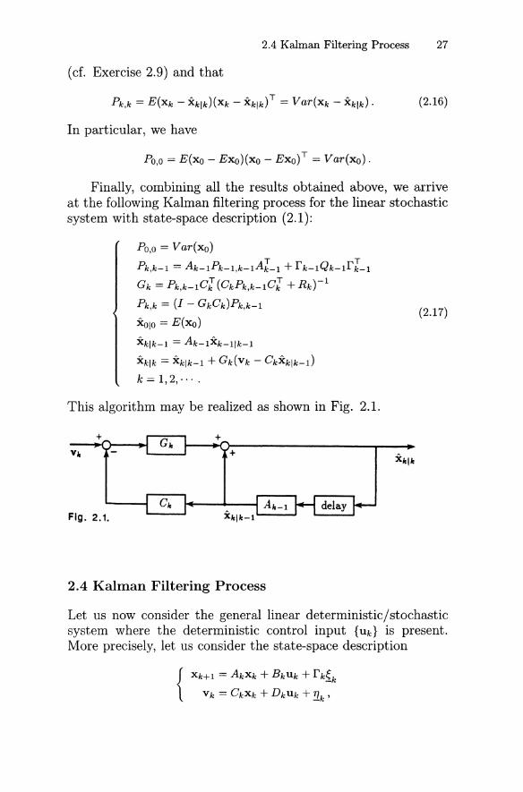
Finally, combining all the results obtained above, we arriveat the following Kalman filtering process for the linear stochasticsystem with state-space description (2.1):
Po,o = Var(xo)
Pk,k-l = Ak-lPk-l,k-lAr-l + rk-lQk-lrr-l
Gk = Pk,k-lC"[ (CkPk,k-lC"[ + Rk)-l
Pk,k = (I - GkCk)Pk,k-l
xOlo = E(xo)
xklk-l = Ak-lXk-llk-l
xklk = xklk-l + Gk(Vk - CkXk1k-l)
k = 1,2,··· .
This algorithm may be realized as shown in Fig. 2.1.
(2.17)
+
Fig. 2.1.
2.4 Kalman Filtering Process
Let us now consider the general linear deterministic/stochasticsystem where the deterministic control input {Uk} is present.More precisely, let us consider the state-space description
{
Xk+l = AkXk + BkUk + rk~k
Vk = CkXk + DkUk +!1k'
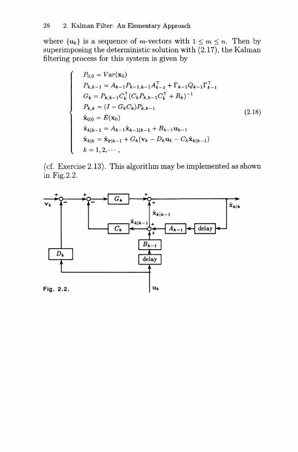
28 2. Kalman Filter: An Elementary Approach
where {Uk} is a sequence of m-vectors with 1 ~ m ~ n. Then bysuperimposing the deterministic solution with (2.17), the Kalmanfiltering process for this system is given by
Po,o == Var(xo)
Pk,k-l == Ak-1Pk-l,k-lAJ-l + rk-1Qk-lrJ-l
Gk == Pk,k-lC~ (CkPk,k-lC~ + Rk)-l
Pk,k == (I - GkCk)Pk,k-l
xOlo == E(xo)
xklk-l == Ak-lXk-llk-l + Bk-lUk-l
xklk == Xk/k-l + Gk(Vk - DkUk - CkXk1k-l)
k == 1,2,,,,,
(2.18)
(cf. Exercise 2.13). This algorithm may be implemented as shownin Fig.2.2.
Fig. 2.2.
Exercises 29
Exercises
2.1. Let
[ :~:,o.]fk,j = c
-k,J
andk
£k,l = '0. - Cl L ~liri-1Si_1'i=l+l
where {Sk} and {!lk} are both zero-mean Gaussian whitenoise sequences with Var(Sk) = Qk and Var(!lk) = Rk. DefineWk,j = (Var(fk,j))-l. Show that
W- 1k,k-1 =
and
o ] [CO 2::=1 ~Oiri-1Si_1 ]+Var :
Rk-1 Ck-1 ~k-1,krk-1Sk_1
W - 1 _ [Wk-~-l 0]k,k - b Rk'
2.2. Show that the sum of a positive definite matrix A and anon-negative definite matrix B is positive definite.
2.3. Let fk,j and Wk,j be defined as in Exercise 2.1. Verify therelation
where
and then show that
W~~_l = Wk!1,k-1 +Hk-1,k-1~k-1,krk-1Qk-1rr-1~r-1,kH;[-1,k-1.
2.4. Use Exercise 2.3 and Lemma 1.2 to show that
Wk,k-1 =Wk-1,k-1 - Wk-1,k-1Hk-1,k-1~k-1,krk-1(Qk~1
+ rl-1~l-1,kH"[-1,k-1Wk-1,k-1Hk-1,k-1 ~k-1,krk-1)-1
. rl-1~l-1,kH"[-1,k-1Wk-1,k-1 .
2.5. Use Exercise 2.4 and the relation Hk,k-1 = Hk-1,k-1~k-1,k toshow that
H~k-1Wk,k-1
=~l-l,k{I - H;[-1,k-1Wk-1,k-1Hk-1,k-1 ~k-1,krk-1(Qk~l
+ rl-1~l-1,kHI-1,k-1Wk-1,k-1Hk-1,k-1 ~k-1,krk-1)-1
. rl- 1~r-1,k}HI-1,k-1Wk-1,k-1 .
30 2. Kalman Filter: An Elementary Approach
2.6. Use Exercise 2.5 to derive the identity:
(H~k-1Wk,k-1Hk,k-1)<I>k,k-1 (H"[-1,k-1 Wk-1,k-1Hk-1,k-1)-1
. H"[-1,k-1 Wk-1,k-1 = H~k-1Wk,k-1 .
2.7. Use Lemma 1.2 to show that
Pk,k-1C"[ (CkPk,k-1C"[ + Rk)-l = Pk,kC"[ Rk1 = Gk.
2.8. Start with Pk,k-1 = (H"[k-1Wk,k-1Hk,k-1)-1. Use Lemma 1.2,(2.8), and the definiti~n of Pk,k = (H~kWk,kHk,k)-l to showthat
Pk,k-1 = Ak-1Pk-1,k-1Al-1 + rk-1Qk-1rl-1 .
2.9. Use (2.5) and (2.2) to prove that
E(Xk - xklk-1)(Xk - xklk-1) T = Pk,k-1
andE(Xk - xklk)(Xk - xklk) T = Pk,k .
2.10. Consider the one-dimensional linear stochastic dynamicsystem
Xo = 0,
where E(Xk) = 0, Var(xk) = 0-2, E(Xk~j) = 0, E(~k) = 0, andE(~k~j) = J-L28kj. Prove that 0-2 = J-L2/(1 - a2) and E(XkXk+j) =a1j1 0-2 for all integers j.
2.11. Consider the one-dimensional stochastic linear system
with E(TJk) = 0, Var(TJk) = 0-2,E(xo) = °and Var(xo) = J-L2.Show that
and that xklk -t c for some constant c as k -t 00.
2.12. Let {Vk} be a sequence of data obtained from the observation of a zero-mean random vector y with unknown varianceQ. The variance of y can be estimated by
Exercises 31
Derive a prediction-correction recursive formula for this estimation.
2.13. Consider the linear deterministic/stochastic system
{
Xk+l = AkXk + BkUk + rk~k
Vk = CkXk + Dk Uk + '!lk '
where {Uk} is a given sequence of deterministic control inputm-vectors, 1 :::; m :::; n. Suppose that Assumption 2.1 issatisfied and the matrix Var(?k,j) is nonsingular (cf. (2.2) forthe definition of "fk,j). Derive the Kalman filtering equationsfor this model.
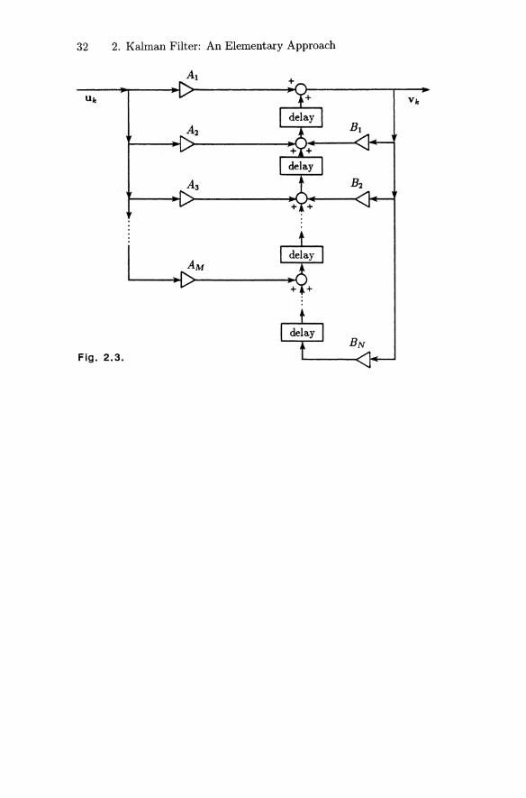
2.14. In digital signal processing, a widely used mathematical model is the following so-called ARMA (autoregressivemoving-average) process:
N M
Vk = L BiVk-i + L AiUk-i ,i=l i=O
where the n x n matrices B I ,'" ,BN and the n x q matricesAo, AI,"', AM are independent of the time variable k, and{Uk} and {Vk} are input and output digital signal sequences,respectively (cf. Fig. 2.3). Assuming that M :::; N, showthat the input-output relationship can be described as astate-space model
{
Xk+l = AXk + BUk
Vk = CXk + DUk
with Xo = 0, where
Al + BIAoB I I 0 0 A 2 + B 2 Ao
B 2 0 IA= B= AM+BMAo
BN-I 0 I BM+IAo
BN 0 0BNAo
C=[10"'0] and D = [Ao] .
32 2. Kalman Filter: An Elementary Approach
At
Fig. 2.3.
3. Orthogonal Projection and Kalman Filter
The elementary approach to the derivation of the optimal Kalmanfiltering process discussed in Chapter 2 has the advantage thatthe optimal estimate Xk == xklk of the state vector Xk is easilyunderstood to be a least-squares estimate of Xk with the properties that (i) the transformation that yields Xk from the dataVk == [vci··· vl]T is linear, (ii) Xk is unbiased in the sense thatE(Xk) == E(Xk), and (iii) it yields a minimum variance estimatewith (VarCfk,k))-l as the optimal weight. The disadvantage of thiselementary approach is that certain matrices must be assumedto be nonsingular. In this chapter, we will drop the nonsingularity assumptions and give a rigorous derivation of the Kalmanfiltering algorithm.
3.1 Orthogonality Characterizationof Optimal Estimates
Consider the linear stochastic system described by (2.1) such thatAssumption 2.1 is satisfied. That is, consider the state-spacedescription
{
Xk+l == AkXk + rk{k(3.1)
Vk == CkXk + !1.k '
where Ak , rk and Ok are known n x n, n x p and q x n constantmatrices, respectively, with 1 ::; p, q ::; n, and
E({k) == 0, E(~k~;) == Qk8kl,
E({kTlJ) == 0, E(xo~~) == 0, E(xo!1.~) == 0,
for all k, f == 0,1,···, with Qk and Rk being positive definite andsymmetric matrices.
Let x be a random n-vector and w a random q-vector. Wedefine the "inner product" (x, w) to be the n x q matrix
34 3. Orthogonal Projection and Kalman Filter
(x, w) = Cov(x, w) = E(x - E(x))(w - E(w))T .
Let Ilwllq be the positive square root of (w, w). That is, IIwllq is anon-negative definite q x q matrix with
IIwll~ = Ilwllqllwll; = (w, w).
Similarly, let IIxlln be the positive square root of (x, x). Now, letwo,' . " W r be random q-vectors and consider the "linear span":
Y(wo,"', w r )
r
={y: y = L Piwi, Po,"', Pr, n x q constant matrices}.i=o
The first minimization problem we will study is to determine a yin Y(wo,"', w r ) such that trllxk - yll~ = Fk' where
Fk := min{trllxk - yll~: y E Y(wo,"', w r )}. (3.2)
The following result characterizes y.
Lemma 3.1. y E Y(wo,"', w r ) satisfies trllxk - yll~ = Fk if andonly if
(Xk - y, Wj) = Onxq
for all j = 0, 1, ... , r. Furthermore, y is unique in the sense that
trllxk - YII~ = trllxk - YII;only ify = y.
To prove this lemma, we first suppose that trllxk - yll~ = Fkbut (Xk - y, Wjo) = C =I- Onxq for some jo where 0 :::; jo :::; r. ThenWjo =I- 0 so that Ilwjoll~ is a positive definite symmetric matrixand so is its inverse Ilwjoll~2. Hence, Cllwjoll~2CT =1= Onxn and isa non-negative definite and symmetric matrix. It can be shownthat
tr{Cllwjoll;2CT} > 0 (3.3)
(cf. Exercise 3.1). Now, the vector y + Cllwjoll~2wjo is in Y(wo,
"', w r ) and
trllxk - (y + Cllwjoll;2Wjo)ll~
= tr{lI x k - YII; - (Xk - y, wjo)(Cllwjoll;2)T - Cllwjoll;2(wjo,Xk - y)
+ Cllwjo 11;211 w jo 11~(Cllwjo11;2)T}
= tr{llxk - :9"11; - CIIWjoll;2CT}
< trllxk - :9"11; = F k
by using (3.3). This contradicts the definition of Fk in (3.2).
3.2 Innovations Sequences 35
Conversely, let (Xk -Y, Wj) = Onxq for all j = 0,1" . " r. Let y bean arbitrary random n-vector in Y(wo,"" w r ) and write Yo = y
Y= 2:j=o PojWj where Poj are constant nxq matrices, j = 0,1"", r.
Then
trllxk - yll;= trll(xk - y) - Yoll;
= tr{lI xk - YII; - (Xk - Y, Yo) - (Yo, Xk - y) + IIYoll;}
= tr{llxk -Yll;' - t(Xk -y,Wj)P;;j - tPOj(Xk _y,Wj)T + IIYolI;'})=0 )=0
= trllxk - YII; + trllYoll;
2: trllxk - YII; ,
so that trllxk - yll~ = Fk. Furthermore, equality is attained if andonly if trllYoll~ = 0 or Yo = 0 so that Y = Y(cf. Exercise 3.1). Thiscompletes the proof of the lemma.
3.2 Innovations Sequences
To use the data information, we require an "orthogonalization"process.
Definition 3.1. Given a random q-vector data sequence {Vj},
j = O,···,k. The innovations sequence {Zj}' j = O, .. ·,k, of {Vj}
(i.e., a sequence obtained by changing the original data sequence{ v j }) is defined by
Zj=Vj-CjYj_1' j=O,l,···,k,
with Y-1 = 0 and
j-1
Yj-1 = L Pj-1,iV i E Y(vo,"', Vj_1) , j = 1"", k,i=o
(3.4)
where the q x n matrices Cj are the observation matrices in (3.1)and the n x q matrices Pj - 1,i are chosen so that Yj-1 solvesthe minimization problem (3.2) with Y(wo,"', w r ) replaced byY(vo,"', Vj_1)'
We first give the correlation property of the innovations sequence.
36 3. Orthogonal Projection and Kalman Filter
Lemma 3.2. The innovations sequence {Zj} of {Vj} satisfies thefollowing property:
(Zj,Zf) = (Ri + Clllxl - Yl-lll~CJ)8jl,
where Ri = Var('!lt) > O.
For convenience, we set
ej = Cj(Xj - Yj-l)'
To prove the lemma, we first observe that
Zj = ej + '!1j'
where {'!1k} is the observation noise sequence, and
('!It' ej) = Oqxq for all f 2 j .
(3.5)
(3.6)
(3.7)
Clearly, (3.6) follows from (3.4), (3.5), and the observation equation in (3.1). The proof of (3.7) is left to the reader as an exercise(cf. Exercise 3.2). Now, for j = f, we have, by (3.6), (3.7), and(3.5) consecutively,
(Zl, Zi) = (el + '!It' ei + '!It)
= (el, el) + (!It' !il)
= Cl\\Xl - Yl-ll1~cJ + Ri·
For j =I f, since (ei,ej)T = (ej,ei)' we can assume without loss ofgenerality that j > f. Hence, by (3.6), (3.7), and Lemma 3.1 wehave
(Zj, Zl) = (ej, el) + (ej, "70) + ("7., el) + (7J., "70)~ -J -J ~
= (ej, ei + '!It)= (ej, Zi)
= (ej, Vi - CiYi-l)
/ i-I)= \ Cj(Xj - Yj-l), ve - Ce ~.f>e-l,ivi
2=0i-I= Cj(Xj - Yj-l, Vi) - Cj L(Xj - Yj-l, Vi)Pl~l,iCJ
i=o= Oqxq.
This completes the proof of the lemma.
3.3 Minimum Variance Estimates 37
Since Rj > 0, Lemma 3.2 says that {Zj} is an "orthogonal"sequence of nonzero vectors which we can normalize by setting
(3.8)
Then {ej} is an "orthonormal" sequence in the sense that (ei' ej) =bij Iq for all i and j. Furthermore, it should be clear that
(3.9)
(cf. Exercise 3.3).
3.3 Minimum Variance Estimates
We are now ready to give the minimum variance estimate Xk ofthe state vector Xk by introducing the "Fourier expansion"
k
Xk = L(Xk' ei)eii=o
(3.10)
of Xk with respect to the "orthonormal" sequence {ej}' Since
k
(xk,ej) = L(xk,ei)(ei,ej) = (xk,ej)'i=o
we have(Xk-Xk,ej)=Onxq, j=O,l,···,k.
It follows from Exercise 3.3 that
so that by Lemma 3.1,
That is, Xk is a minimum variance estimate of Xk.
(3.11 )
(3.12)
38 3. Orthogonal Projection and Kalman Filter
3.4 Kalman Filtering Equations
This section is devoted to the derivation of the Kalman filteringequations. From Assumption 2.1, we first observe that
(cf. Exercise 3.4), so that
k
Xk = L(xk,ej)ejj=ok-l
= L(xk,ej)ej + (xk,ek)ekj=ok-l
= L {(Ak-lXk-l, ej )ej + (rk-l~k_l' ej )ej} + (Xk, ek)ekj=o
k-l
= Ak- 1 L(xk-l,ej)ej + (xk,ek)ekj=o
= Ak-1Xk-l + (Xk' ek)ek .
Hence, by definingXklk-l = Ak-lXk-l ,
where Xk-l := Xk-llk-l, we have
(3.13)
(3.14)
Obviously, if we can show that there exists a constant n x q matrixGk such that
(xk,ek)ek = Gk(Vk - CkXk1k-l) '
then the "prediction-correction" formulation of the Kalman filteris obtained. To accomplish this, we consider the random vector(Vk - CkXklk-l) and obtain the following:
Lemma 3.3. For j = 0,1, ... ,k,
To prove the lemma, we first observe that
(3.15)
3.4 Kalman Filtering Equations 39
(cf. Exercise 3.4). Hence, using (3.14), (3.11), and (3.15), wehave
(Vk - CkXklk-1 ,ek)
= (Vk - Ck(Xklk - (Xk, ek)ek), ek)
= (Vk' ek) - Ck{ (xklk, ek) - (Xk, ek)}
= (vk,ek) - Ck(Xklk - xk,ek)
= (Vk' ek)
= (Zk + CkYk-1, Il zkll;lzk)= (Zk, Zk) IIzkll;l + Ck(Yk-1, Zk) IIZk 11;1= II Z kllq·
On the other hand, using (3.14), (3.11), and (3.7), we have
(Vk - Ck Xk1k -1,ej)
= (CkXk +'!lk - Ck(Xklk - (xk,ek)ek),ej)
= Ck (Xk - Xklk, ej) + ('!lk' ej) + Ck(Xk, ek) (ek' ej)
= Oqxq
for j = 0,1,···, k - 1. This completes the proof of the Lemma.
It is clear, by using Exercise 3.3 and the definition of Xk-1 =Xk-1Ik-1, that the random q-vector (Vk-CkXklk-1) can be expressedas I:i=o Miei for some constant q xq matrices Mi. It follows nowfrom Lemma 3.3 that for j = 0,1,· .. ,k,
so that Mo = M1 = ... = Mk-l = 0 and Mk = IIzkllq. Hence,
Define
Then we obtain
(Xk,ek)ek = Gk(Vk - CkXklk-l).
This, together with (3.14), gives the "prediction-correction"equation:
(3.16)
40 3. Orthogonal Projection and Kalman Filter
We remark that xklk is an unbiased estimate of Xk by choosingan appropriate initial estimate. In fact,
Xk - xklk
==Ak-1Xk-l + rk-l~k_l - Ak-lXk-llk-l - Gk(Vk - CkAk-lXk-llk-l) .
Xk - xklk
==(1 - GkCk)Ak-l(Xk-l - Xk-llk-l)
+ (I - GkCk)rk-l~k_l - Gk'!lk .
Since the noise sequences are of zero-mean, we have
so that
Hence, if we set
(3.17)
XOIO == E(xo) , (3.18)
then E(Xk - xklk) == 0 or E(Xklk) == E(Xk) for all k, Le., xklk is indeedan unbiased estimate of Xk.
Now what is left is to derive a recursive formula for Gk. Using(3.12) and (3.17), we first have
o == (Xk - xklk, Vk)
== ((I - GkCk)Ak-l(Xk-l - Xk-llk-l) + (I - GkCk)rk-l~k_l - Gk'!lk'
CkAk-l((Xk-l - Xk-llk-l) + Xk-llk-l) + Ckrk-l~k_l + '!lk)v v 2 T T
== (I - GkCk)Ak-lllxk-l - Xk-llk-lllnAk-l Ckv T T v+ (I - GkCk)rk-lQk-lrk_lck - GkRk, (3.19)
where we have used the facts that (Xk-l -Xk-llk-l' Xk-llk-l) == Onxn,a consequence of Lemma 3.1, and
(Xk'~k) == Onxn,
(Xk'!lj) == Onxq ,
(Xklk' €.) == Onxn ,-J
(Xk-llk-l, !lk) == Onxq ,(3.20)
j == 0, ... , k (cf. Exercise 3.5). Define
Pk,k == Ilxk - xklkll;
3.4 Kalman Filtering Equations 41
andPk,k-l = Ilxk - xklk-lll~·
Then again by Exercise 3.5 we have
Pk,k-l = IIAk-1Xk-l + rk-l~k_l - Ak-lXk-llk-lll~
= Ak-1\lxk-l - Xk-llk-lll~Al-l + rk-lQk-lrl-l
orPk,k-l = Ak-1Pk-l,k-lAl-..l +rk-lQk-lrl-l' (3.21)
On the other hand, from (3.19), we also obtainv T T
(I - GkCk)Ak-lPk-l,k-lAk-lCkv T T v+ (I - GkCk)rk-lQk-lrk_lCk - GkRk = o.
In solving for Ok from this expression, we writev T T T
Gk[Rk + Ck(Ak-1Pk-l,k-lAk-l + rk-1Qk-lrk-l)Ck ]
= [Ak-lPk-l,k-lAl-l + rk-lQk-lrl-l]C~
= Pk,k-lC~ .
and obtainv T T 1
Gk = Pk,k-lCk (Rk + CkPk,k-lCk)- , (3.22)
where Rk is positive definite and CkPk,k-lC~ is non-negative definite so that their sum is positive definite (cf. Exercise 2.2).
Next, we wish to write Pk,k in terms of Pk,k-l, so that togetherwith (3.21), we will have a recursive scheme. This can be doneas follows:
Pk,k = II x k - xklkll~
= Ilxk - (xklk-l + Ok(Vk - Ckxklk-l))II~v v 2
= Ilxk - xklk-l - Gk(CkXk + '!lk) + GkCkxklk-lllnv v 2
= 11(1 - GkCk)(Xk - xklk-l) - Gk!lkllnv 2 v T v VT
= (I - GkCk)\Ixk - xklk-llln(1 - GkCk) + GkRkG kv v T v VT
= (I - GkCk)Pk,k-l(1 - GkCk) + GkRkGk ,
where we have applied Exercise 3.5 to conclude that (Xk xklk-l,!lk) = Onxq. This relation can be further simplified by using(3.22). Indeed, since
(3.25)
42 3. Orthogonal Projection and Kalman Filter
we have.... v T.... .... T
Pk,k ==(1 - GkCk)Pk,k-l(I - GkCk) + (I - GkCk)Pk,k-l(GkCk)
==(1 - OkCk)Pk,k-l . (3.23)
Therefore, combining (3.13), (3.16), (3.18), (3.21), (3.22) and(3.23), together with
Po,o == IIxo - xOloll~ == Var(xo) , (3.24)
we obtain the Kalman filtering equations which agree with theones we derived in Chapter 2. That is, we have xklk == xklk' xklk-l ==xklk-l and Ok == Gk as follows:
Po,o == Var(xo)
Pk,k-l == Ak-lPk-l,k-lAl-l + fk-lQk-lfr-l
Gk == Pk,k-l C-:' (CkPk,k-1C-:' + Rk)-l
Pk,k == (I - GkCk)Pk,k-l
xOlo == E(xo)
xklk-l == Ak-1Xk-llk-l
xklk == xklk-l + Gk(Vk - CkXk1k-l)k == 1,2, ....
Of course, the Kalman filtering equations (2.18) derived inSection 2.4 for the general linear deterministic/stochastic system
{
Xk+l == AkXk + BkUk + rk~k
Vk == CkXk + DkUk +!1k
can also be obtained without the assumption on the invertibilityof the matrices Ak, VarC~k,j)' etc. (cf. Exercise 3.6).
3.5 Real-Time Tracking
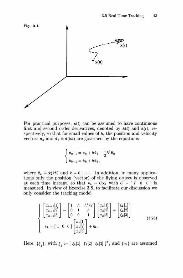
To illustrate the application of the Kalman filtering algorithm described by (3.25), let us consider an example of real-time tracking.Let x(t), 0 :::; t < 00, denote the trajectory in three-dimensionalspace of a flying object, where t denotes the time variable (cf.Fig.3.1). This vector-valued function is discretized by samplingand quantizing with sampling time h > 0 to yield
Xk ~ x(kh), k == 0,1,···.
3.5 Real-Time 'fracking 43
Fig. 3.1.
-~, ", - - x(t)
"'-,I
I
• x(O)
For practical purposes, x(t) can be assumed to have continuousfirst and second order derivatives, denoted by x(t) and x(t), respectively, so that for small values of h, the position and velocityvectors Xk and Xk ~ x(kh) are governed by the equations
{
h · 1h2 ..~k+l = ~k + ~k +"2 Xk
Xk+l = Xk + hXk ,
where Xk ~ x(kh) and k = 0,1,···. In addition, in many applications only the position (vector) of the flying object is observedat each time instant, so that Vk = CXk with C = [I 0 0] ismeasured. In view of Exercise 3.8, to facilitate our discussion weonly consider the tracking model
(3.26)
44 3. Orthogonal Projection and Kalman Filter
to be zero-mean Gaussian white noise sequences satisfying:
E(~k) = 0, E("1k) = 0,
E(~k~;) = Qk6kl, E("1k"1l) = rk6kl,
E(xo~;) = 0, E(Xo"1k) = 0,
where Qk is a non-negative definite symmetric matrix and rk > 0for all k. It is further assumed that initial conditions E(xo) andVar(xo) are given. For this tracking model, the Kalman filteringalgorithm can be specified as follows: Let Pk := Pk,k and let P[i, j]denote the (i, j)th entry of P. Then we have
Pk,k-l[l,l] = Pk-l[l, 1] + 2hPk-l[1, 2] + h2Pk_l[1, 3] + h2Pk-l[2, 2]
h4
+ h3Pk-l[2, 3] + 4Pk-1[3, 3] + Qk-l[l, 1],
Pk,k-l[1,2] = Pk,k-l[2, 1]
3h2
= Pk-l[l, 2] + hPk-l[l, 3] + hPk-l[2, 2] + TPk-1[2, 3]
h3
+ 2Pk-1[3, 3] + Qk-l[l, 2],
Pk,k-l[2,2] = Pk-l[2, 2] + 2hPk-l[2, 3] + h2Pk-l[3, 3] + Qk-l[2, 2],
Pk,k-l[1,3] = Pk,k-l[3, 1]
h2
= Pk- 1[1, 3] + hPk- 1[2, 3] + 2Pk-1[3, 3] + Qk-l[l, 3],
Pk,k-l [2,3] = Pk,k-l [3,2]= Pk-l[2, 3] + hPk-l[3, 3] + Qk-l[2, 3],
Pk,k-l [3,3] = Pk-l [3,3] + Qk-l [3,3] ,
with Po,o = Var(xo) ,
with :Kala = E(xo).
Exercises
Exercises 45
(3.27)
3.1. Let A =f. 0 be a non-negative definite and symmetric constantmatrix. Show that trA > o. (Hint: Decompose A as A = BBT
with B =f. 0.)3.2. Let
j-I
ej = Cj(Xj - Yj-I) = C j (Xi - L Pi-l,iVi) ,'1.=0
where Pj-I,i are some constant matrices. Use Assumption 2.1to show that
for all /!, ? j.3.3. For random vectors WO,"', W r , define
Y(Wo,"', w r )
r
y= LPiWi,i=O
Po, ... 'Pr' constant matrices}.
Letj-I
Zj = Vj - C j L Pj-l,iVi
i=O
be defined as in (3.4) and ej = Ilzjll-lzj' Show that
3.4. Letj-I
Yj-I = L Pj-l,iVi
i=O
andj-I
Zj = Vj - C j L Pj-l,iVi .
i=O
Show that
j = 0,1," . ,k - 1.
46 3. Orthogonal Projection and Kalman Filter
3.5. Let ej be defined as in Exercise 3.3. Also define
k
Xk == L(Xk, ei)eii=O
as in (3.10). Show that
(Xk, "l.) == Onxq ,-J
for j == O,l,···,k.3.6. Consider the linear deterministic/stochastic system
{Xk+l == AkXk + BkUk + rk{k
Vk == CkXk + DkUk +!lk '
where {Uk} is a given sequence of deterministic control inputm-vectors, 1 :::; m :::; n. Suppose that Assumption 2.1 is satisfied. Derive the Kalman filtering algorithm for this model.
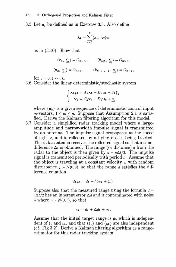
3.7. Consider a simplified radar tracking model where a largeamplitude and narrow-width impulse signal is transmittedby an antenna. The impulse signal propagates at the speedof light c, and is reflected by a flying object being tracked.The radar antenna receives the reflected signal so that a timedifference b..t is obtained. The range (or distance) d from theradar to the object is then given by d == c~t/2. The impulsesignal is transmitted periodically with period h. Assume thatthe object is traveling at a constant velocity w with randomdisturbance ~ ~ N(O, q), so that the range d satisfies the difference equation
dk+1 == dk + h(Wk + ~k) .
Suppose also that the measured range using the formula d ==cb..t/2 has an inherent error ~d and is contaminated with noise"l where "l~N(O,r), so that
Assume that the initial target range is do which is independent of ~k and "lk, and that {~k} and {"lk} are also independent(cf. Fig.3.2). Derive a Kalman filtering algorithm as a rangeestimator for this radar tracking system.
radar
Exercises 47
Fig. 3.2.
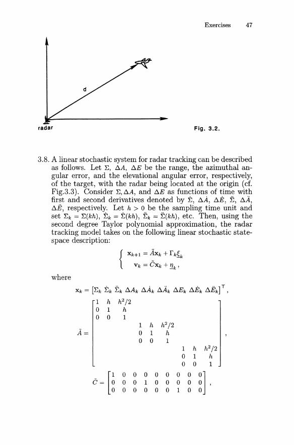
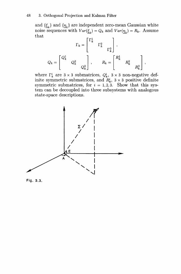
3.8. A linear stochastic system for radar tracking can be describedas follows. Let E, ~A, ~E be the range, the azimuthal angular error, and the elevational angular error, respectively,of the target, with the radar being located at the origin (cf.Fig.3.3). Consider E, ~A, and ~E as functions of time withfirst and second derivatives denoted by E, ~A, ~E, ~, ~A,
~E, respectively. Let h > 0 be the sampling time unit andset Ek = E(kh), Ek = E(kh), Ek = E(kh), etc. Then, using thesecond degree Taylor polynomial approximation, the radartracking model takes on the following linear stochastic statespace description:
{Xk+l = AXk + rk~k
Vk = CXk + '!lk'
where
Xk = [Ek Ek Ek ~Ak ~Ak ~Ak ~Ek ~Ek ~Ek] T ,
1 h h2 /2o 1 ho 0 1
1 h h2 /2o 1 ho 0 1
1 h h2 /20 1 h0 0 1
C = [~0 0 0 0 0 0 0
~] ,0 0 1 0 0 0 00 0 0 0 0 1 0
48 3. Orthogonal Projection and Kalman Filter
and {{k} and {!lk} are independent zero-mean Gaussian whitenoise sequences with Var({k) = Qk and Var(!lk) = Rk. Assumethat [fI
f~] ,rk
= k r 2k
[QI
Q~] ,[RI
Rf] ,Qk = k Q~ Rk = k R2
k
where r~ are 3 x 3 submatrices, Q~, 3 x 3 non-negative definite symmetric submatrices, and Rl, 3 x 3 positive definitesymmetric submatrices, for i = 1, 2, 3. Show that this system can be decoupled into three subsystems with analogousstate-space descriptions.
Fig. 3.3.
4. Correlated Systemand Measurement Noise Processes
In the previous two chapters, Kalman filtering for the model involving uncorrelated system and measurement noise processeswas studied. That is, we have assumed all along that
E(~kiJ) = °for k, R = 0,1,' ". However, in applications such as aircraft inertial navigation systems, where vibration of the aircraft induces acommon source of noise for both the dynamic driving system andonboard radar measurement, the system and measurement noisesequences {~k} and {!lk} are correlated in the statistical sense,with
E(~kiJ) = Sk8k£ ,
k,P = 0,1,"', where each Sk is a known non-negative definite matrix. This chapter is devoted to the study of Kalman filtering forthe above model.
4.1 The Affine Model
Consider the linear stochastic state-space description
{Xk+l = AkXk + rk~k
Vk = CkXk + !lk
with initial state Xo, where Ak' Ck and rk are known constantmatrices. We start with least-squares estimation as discussed inSection 1.3. Recall that least-squares estimates are linear functions of the data vectors; that is, if x is the least-squares estimateof the state vector x using the data v, then it follows that x= Hvfor some matrix H. To study Kalman filtering with correlatedsystem and measurement noise processes, it is necessary to extend to a more general model in determining the estimator x. Itturns out that the affine model
x=h+Hv (4.1)
50 4. Correlated Noise Processes
which provides an extra parameter vector h is sufficient. Here, his some constant n-vector and H some constant n x q matrix. Ofcourse, the requirements on our optimal estimate x of x are: x isan unbiased estimator of x in the sense that
E(x) = E(x)
and the estimate is of minimum (error) variance.From (4.1) it follows that
h = E(h) = E(x - Hv) = E(x) - H(E(v)).
Hence, to satisfy the requirement (4.2), we must have
h = E(x) - HE(v).
or, equivalently,x= E(x) - H(E(v) - v) .
(4.2)
(4.3)
(4.4)
On the other hand, to satisfy the minimum variance requirement,we use the notation
F(H) = Var(x - x) = Ilx - xII;,
so that by (4.4) and the fact that Ilvll; = Var(v) is positive definite,we obtain·
F(H) = (x-x,x-x)
= ((x - E(x)) - H(v - E(v)), (x - E(x)) - H(v - E(v)))
= Ilxll; - H(v,x) - (x, v)HT + Hllvll~HT
= {lIxll; - (x,v)[Ilvll~]-l(v,x)}
+ {Hllvll~HT - H(v, x) - (x, v)HT + (x, v)[lIvll~]-l(v, x)}
= {lIxll~ - (x; v) [lIvll~]-l (v, x)}
+ [H - (x, v)[lIvll~]-l]lIvll~[H - (x, v)[lIvll~]-l]T ,
where the facts that (x, v) T = (v, x) and that Var(v) is nonsingularhave been used.
Recall that minimum variance estimation means the existence of H* such that F(H) 2:: F(H*), or F(H) - F(H*) is nonnegative definite, for all constant matrices H. This can be attained by simply setting
H* = (x, v)[Ilvll~]-l , (4.5)
4.2 Optimal Estimate Operators 51
so that
F(H) - F(H*) = [H - (x, v)[llvll~]-l]lIvll~[H - (x, v)[llvll~]-l]T ,
which is non-negative definite for all constant matrices H. Furthermore, H* is unique in the sense that F(H) - F(H*) = 0 if andonly if H = H*. Hence, we can conclude that x can be uniquelyexpressed as
x = h+H*v,
where H* is given by (4.5). We will also use the notation x =L(x, v) for the optimal estimate of x with data v, so that by using(4.4) and (4.5), it follows that this "optimal estimate operator"satisfies:
L(x, v) = E(x) + (x, v)[llvll~]-l(v - E(v)). (4.6)
4.2 Optimal Estimate Operators
First, we remark that for any fixed data vector v, L(·, v) is a linearoperator in the sense that
L(Ax + By, v) = AL(x, v) + BL(y, v) (4.7)
for all constant matrices A and B and state vectors x and y (cf.Exercise 4.1). In addition, if the state vector is a constant vectora, then
L(a, v) = a (4.8)
(cf. Exercise 4.2). This means that if x is a constant vector, sothat E(x) = x, then x = x, or the estimate is exact.
We need some additional properties of L(x, v). For this purpose we first establish the following.
Lemma 4.1. Let v be a given data vector and y = h+Hv, whereh is determined by the condition E(y) = E(x), so that y is uniquelydetermined by the constant matrix H. If x* is one of the y's suchthat
trllx - x*ll~ = mintrllx - YII~,H
then it follows that x* = x, where x= L(x, v) is given by (4.6).
52 4. Correlated Noise Processes
This lemma says that the minimum variance estimate x andthe "minimum trace variance" estimate x* of x from the samedata v are identical over all affine models.
To prove the lemma, let us consider
trllx - YII;== trE((x - y)(x _ y) T)
== E((x - y)T (x - y))
== E((x - E(x)) - H(v - E(v))T ((x - E(x)) - H(v - E(v)),
where (4.3) has been used. Taking
8 28H (trllx - Ylln) == 0,
we arrive at
x* == E(x) - (x, v)[Ilvll~]-l(E(v) - v) (4.9)
which is the same as the x given in (4.6) (cf. Exercise 4.3). Thiscompletes the proof of the Lemma.
4.3 Effect on Optimal Estimation with Additional Data
Now, let us recall from Lemma 3.1 in the previous chapter thaty E Y == Y(wo,"" wr ) satisfies
trllx - YII; == mintrllx - YII;yEY
if and only if
(x-y,Wj)==Onxq, j==O,l,···,r.
Set Y == Y(v - E(v)) and x == L(x, v) == E(x) + H*(v - E(v)), whereH* == (x, v)[llvll~]-l. If we use the notation
x == x - E(x) and v == v - E(v) ,
then we obtain
IIx - xii; == 11 (x - E(x)) - H*(v - E(v))II; == Ilx - H*vll; .
4.3 Effect on Optimal Estimation 53
But H* was chosen such that F(H*) ::; F(H) for all H, and thisimplies that trF(H*) ::; trF(H) for all H. Hence, it follows that
trllx - H*vll; ::; trllx - YII;
for all Y E Y(v - E(v)) = y(v). By Lemma 3.1, we have
(x - H*v, v) = Onxq .
Since E(v) is a constant, (x - H*v, E(v)) = Onxq, so that
(x - H*v, v) = Onxq ,
or(x - x, v) = Onxq .
Consider two random data vectors vI and v 2 and set
(4.10)
(4.11)
Then from (4.10) and the definition of the optimal estimate operator L, we have
(4.12)
and similarly,(v2#, vI) = o. (4.13)
The following lemma is essential for further investigation.
Lemma 4.2. Let x be a state vector and vI, v 2 be randomobservation data vectors with nonzero finite variances. Set
Then the minimum variance estimate x of x using the data v canbe approximated by the minimum variance estimate L(x, vI) of xusing the data vI in the sense that
with the error
e(x,v2) :=L(x#,v2#)
= (x#, v 2#)[llv2#11 2]-Iv 2# .
(4.14)
(4.15)
54 4. Correlated Noise Processes
We first verify (4.15). Since L(x,y1) is an unbiased estimateof x (cf. (4.6)),
E(x#) = E(x - L(x, yl)) = o.
Similarly, E(y2#) = o. Hence, by (4.6), we have
L(x#, y2#) = E(x#) + (x#, y2#) [Il y2# 11 2]-I(y2# - E(y2#))
= (x#,y2#)[lIy2#1I 2]-ly2#,
yielding (4.15). To prove (4.14), it is equivalent to showing that
XO := L(x, yl) + L(x# ,y2#)
is an affine unbiased minimum variance estimate of x from thedata y, so that by the uniqueness of x, XO = X = L(x, v). First,note that
XO = L(x, yl) + L(x#, y2#)
= (hI + H1y l) + (h2 + H2(y2 - L(y2, yl))
= (hI + H1yl) + h2 + H2(y2 - (h3 + H3yl))
= (hI + h 2 - H2h3 ) + H [ :~ ]
:= h+Hy,
where H = [HI - H2 H3 H2 ]. Hence, XO is an affine transformationof Y. Next, since E(L(x, yl)) = E(x) and E(L(x#, y2#)) = E(x#) = 0,we have
E(xO) = E(L(x, yl)) + E(L(x#, y2#)) = E(x).
Hence, XO is an unbiased estimate of x. Finally, to prove thatXO is a minimum variance estimate of x, we note that by usingLemmas 4.1 and 3.1, it is sufficient to establish the orthogonalityproperty
(x-XO,y) =Onxq.
This can be done as follows. By (4.15), (4.11), (4.12), and (4.13),we have
(x - xO, y)
= (x# - (x#,y2#)[lIy 2#11 2]-ly2#,y)1 1
= (x#, [:2]) - (x#,v2#Hllv2#112j-l(v2#, [:2])= (x#, y2) _ (x#, v 2#) [ll y2# 11 2]-1 (y2#, y2) .
(4.16)
4.4 Kalman Filtering Equations 55
But since v 2 = v 2# + L(v2 , vI), it follows that
(v2#,v2) = (v2#,v2#) + (v2#,L(v2,vl ))
from which, by using (4.6), (4.13), and the fact that (v2#,E(vl )) =(v2#, E(v2
)) = 0, we arrive at
(v2#, L(v2 , vI))
= (v2#, E(v2 ) + (v2, vl)[llvI1l2]-I(vl - E(vl )))
= ((v2#,vl ) _ (v2#,E(vl)))[llvII12]-I(vl,v2)
=0,
so that(v2#, v 2) == (v2#, v 2#) .
Similarly, we also have
(x#, v 2) = (x#, v 2#) .
Hence, indeed, we have the orthogonality property:
(x - xo, v)
=(x#,v2#) - (x#,v2#)[Ilv2#112]-I(v2#,v2#)
==Onxq.
This completes the proof of the Lemma.
4.4 Derivation of Kalman Filtering Equations
We are now ready to study Kalman filtering with correlated system and measurement noises. Let us again consider the linearstochastic system described by
{
Xk+1 = AkXk + rk~k
Vk = CkXk + '!lk
with initial state Xo, where Ak, Ck and rk are known constantmatrices. We will adopt Assumption 2.1 here with the exceptionthat the two noise sequences {~k} and {'!lk} may be correlated,namely: we assume that {~k} and {'!lk} are zero-mean Gaussianwhite noise sequences satisfying
E(~kXci) = Opxn , E('!lkxci ) = Oqxn ,
E(~k~;) == Qk8kl , E('!lkiJ) == Rk8kl ,E(~kiJ) = Sk8kl ,
56 4. Correlated Noise Processes
where Qk, Rk are, respectively, known non-negative definite andpositive definite matrices and Sk is a known, but not necessarilyzero, non-negative definite matrix.
The problem is to determine the optimal estimate Xk = xklkof the state vector Xk from the data vectors Vo, VI,···, Vk, usingthe initial information E(xo) and Var(xo). We have the followingresult.
Theorem 4.1. The optimal estimate Xk = xklk of Xk from thedata vo, VI,···, Vk can be computed recursively as follows: Define
Po,o = Var(xo) .
Then, for k = 1,2, ... , compute
Pk,k-I =(Ak- I - Kk-ICk-I)Pk-l,k-I(Ak-1 - Kk-ICk-l) T
+ rk-IQk-Irl-1 - Kk-IRk-IKl-I , (a)
where(b)
and the Kalman gain matrix
withPk,k = (I - GkCk)Pk,k-1 .
Then, with the initial condition
xOlo = E(xo) ,
compute, for k = 1,2,· .. , the prediction estimates
(c)
(d)
and the correction estimates
(cf. Fig.4.1).
(f)
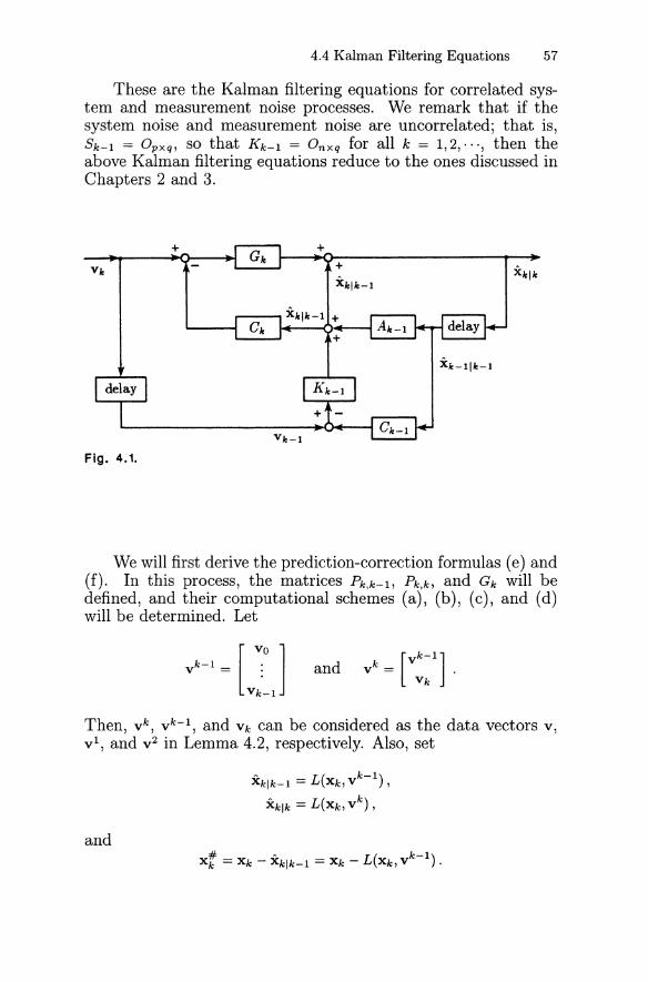
4.4 Kalman Filtering Equations 57
These are the Kalman filtering equations for correlated system and measurement noise processes. We remark that if thesystem noise and measurement noise are uncorrelated; that is,Sk-I = Opxq, so that Kk-I = Onxq for all k = 1,2,···, then theabove Kalman filtering equations reduce to the ones discussed inChapters 2 and 3.
+
Fig. 4.1.
We will first derive the prediction-correction formulas (e) and(f). In this process, the matrices Pk,k-I, Pk,k, and Gk will bedefined, and their computational schemes (a), (b), (c), and (d)will be determined. Let
Then, v k , V k - I , and Vk can be considered as the data vectors v,VI, and v 2 in Lemma 4.2, respectively. Also, set
A L( k-I)Xklk-I = Xk, v ,
Xklk = L(Xk, v k) ,
and# A L( k-I)X k = Xk - Xklk-I = Xk - Xk, v .
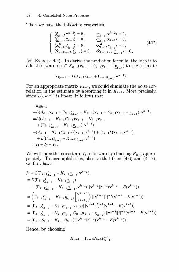
58 4. Correlated Noise Processes
Then we have the following properties
(~k-1'Vk-
2) = 0,
(~k-1'Xk-1) = 0,
(Xt-1'~k_1) = 0,
(Xk-1Ik-2, ~k-1) = 0,
('1k-1' Vk-
2) = 0,
('1k-1' Xk-1) = 0,
(xt-1' '1k-1) = 0,(Xk-1Ik-2, '!lk-1) = 0,
(4.17)
(cf. Exercise 4.4). To derive the prediction formula, the idea is toadd the "zero term" Kk-1(Vk-1 - Ck-1Xk-1 - '!lk-1) to the estimate
For an appropriate matrix Kk-1, we could eliminate the noise correlation in the estimate by absorbing it in Kk-1. More precisely,since L(.,vk - 1 ) is linear, it follows that
Xklk-1
=L(Ak-1Xk-1 + rk-1~k_1 + Kk-1(Vk-1 - Ck-1Xk-1 - '!lk-1)' vk-
1)
=L((Ak- 1 - Kk-1Ck-1)Xk-1 + Kk-1Vk-1
+ (rk-1~k_1 - Kk-1'!1.k_1) , Vk-
1)
=(Ak-1 - Kk-1Ck-1)L(Xk-1, v k- 1) + Kk-1L(Vk-1, Vk- 1)
+ L(rk-1~k_1 - Kk-1'!lk_1' vk
-1
)
:=11 + 12 + 13 .
We will force the noise term 13 to be zero by choosing Kk-1 appropriately. To accomplish this, observe that from (4.6) and (4.17),we first have
13 = L(rk-1~k_1 - Kk-1'!lk_1' v k-
1)
= E(rk-1~k_1 - Kk-1!l.k_1)
+ (rk-1~k_1 - Kk-1!l.k_1' vk-1)[llvk-1112]-1(vk-1 - E(vk- 1))
= (rk-l~k_l - Kk-l!lk_l' [::~:J) [llvk-1112rl(vk-l - E(Vk- 1))
= (rk-1~k_1 - Kk-1!l.k_1' Vk_1)[!Ivk-1112]-1(vk-1 - E(vk- 1))
= (rk-1~k_1 - Kk-1'!lk_1' Ck-lXk-l + '1k-1) [lIvk-1112]-1(vk-l - E(vk- 1))
= (rk-lSk-l - Kk_lRk_l)[llvk-1112]-1(vk-l - E(Vk- 1)).
Hence, by choosing
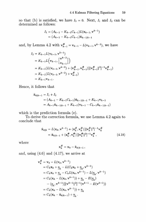
4.4 Kalman Filtering Equations 59
so that (b) is satisfied, we have 13 = o. Next, 11 and 12 can bedetermined as follows:
11 = (Ak- 1 - Kk-1Ck-l)L(Xk-l, v k-
1)
= (Ak- 1 - Kk-1Ck-l)Xk-llk-l
and, by Lemma 4.2 with vt-l = Vk-l - L(Vk-l, vk- 2), we have
12 = Kk-1L(Vk-l, v k-
1)
k-2
= Kk-1L(Vk- 1, [V ])Vk-l
= Kk-l(L(Vk-l, vk- 2) + (vt-l' vt_l)[llvt_11l 2]-lvt_l)
= Kk-1(L(Vk-l, vk- 2) + vt-l)
= Kk-lVk-l.
Hence, it follows that
Xklk-l = 11+ 12
= (Ak-l - Kk-1Ck-l)Xk-llk-l + Kk-lVk-l
= Ak-lXk-llk-l + Kk-l(Vk-l - Ck-1Xk-llk-l)
which is the prediction formula (e).To derive the correction formula, we use Lemma 4.2 again to
conclude that
Xklk = L(Xk,vk- 1) + (xt,vt)[llvtI12]-lvt
= xklk-l + (xt,vt)[llvtIl2]-lvt, (4.18)
where
and, using (4.6) and (4.17), we arrive at
vt = Vk - L(Vk, vk- 1)
= CkXk + ~k - L(CkXk + ~k' vk
-1
)
= CkXk + ~k - CkL(Xk, v k-
1) - L(~k' v k
-1
)
= Ck(Xk - L(Xk, Vk
-1)) + ~k - E('!lk)
- (!1k' vk-l)[lIvk-1112]-1(vk-l - E(vk- 1))
= Ck(Xk - L(Xk, v k-
1)) + ~k
= Ck(Xk - xklk-l) + '!lk .
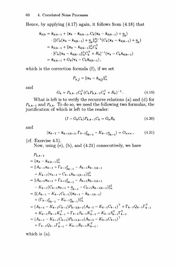
60 4. Correlated Noise Processes
Hence, by applying (4.17) again, it follows from (4.18) that
Xklk == xklk-I + (Xk - xklk-I, Ck(Xk - xklk-I) + !!..k)
. [IICk(Xk - xklk-I) + !lkll~]-I(Ck(xk - xklk-I) + !lk)
== Xk\k-I + IIx k - xk\k-IIl;C~
. [Ckllxk - xklk-III;C~ + Rk]-I(Vk - CkXk1k-l)
== xklk-I + Gk(Vk - CkXk1k-I) '
which is the correction formula (f), if we set
Pk,j == Ilxk - xk1jll;
andGk == Pk,k-IC-: (CkPk,k-IC-: + Rk)-I. (4.19)
What is left is to verify the recursive relations (a) and (d) forPk,k-I and Pk,k. To do so, we need the following two formulas, thejustification of which is left to the reader:
(4.20)
and(Xk-I - Xk-Ilk-I, rk-lik_1 - Kk-l!!..k_l) == Onxn , (4.21)
(cf. Exercise 4.5).Now, using (e), (b), and (4.21) consecutively, we have
Pk,k-I
== II x k - xklk-Ill;
== II A k-I Xk-1 + rk-l~k_1 - Ak-IXk-Ilk-1
- Kk-I(Vk-1 - Ck-IXk-Ilk-I)II;
== IIAk-IXk-1 + rk-l~k_1 - Ak-IXk-Ilk-1
- Kk-I(Ck-IXk-1 + !lk-I - Ck-IXk-Ilk-I)II;
== II(Ak- 1 - Kk-ICk-I)(Xk-1 - Xk-Ilk-I)
+ (rk-l~k_1 - Kk-l!!..k_l) 11;== (Ak- I - Kk-ICk-I)Pk-Ilk-I(Ak-1 - Kk-ICk-l) T + rk-IQk-IrJ-I
+ Kk-IRk-IK-:_I - rk-ISk-IK-:_I - Kk-IS~-lrJ-I
== (Ak- I - Kk-ICk-I)Pk-l,k-1 (Ak- I - Kk-ICk-I) T
+ rk-IQk-IrJ-I - Kk-IRk-IK~_1 ,
which is (a).
(4.22)
4.5 Real-Time Applications 61
Finally, using (f), (4.17), and (4.20) consecutively, we alsohave
Pk,k
= Ilxk - xklkll;
= Ilxk - xklk-l - Gk(Vk - CkXklk-l)ll~
= lI(xk ~ xklk-l) - Gk(CkXk + '!lk - CkXklk-l)ll;
= 11(1 - GkCk)(Xk - xklk-l) - Gk'!lk ll ;
= (1 - GkCk)Pk,k-l(1 - GkCk)T + GkRkGl
= (1 - GkCk)Pk,k-l - (1 - GkCk)Pk,k-lC-:Gl + GkRkGl
= (1 - GkCk)Pk,k-l ,
which is (d). This completes the proof of the theorem.
4.5 Real-Time Applications
An aircraft radar guidance system provides a typical application.This system can be described by using the model (3.26) considered in the last chapter, with only one modification, namely:the tracking radar is now onboard to provide the position datainformation. Hence, both the system and measurement noise processes come from the same source such as vibration, and will becorrelated. For instance, let us consider the following state-spacedescription
[Xk+l[l]] [1 h h
2
/2] [Xk[l]] [~k[l]]Xk+l[2] = 0 1 h xk[2] + ~k[2]
Xk+l[3] 0 0 1 xk[3] ~k[3]
[
Xk[l]]Vk = [1 0 0] xk[2] + TJk ,
xk[3]
where {{k}' with {k := [~k[l] ~k[2] ~k[3]]T, and {TJk} are assumedto be correlated zero-mean Gaussian white noise sequences satisfying
E({k) = 0, E(TJk) = 0,
E({k(;) = Qk6ki!, E(TJkTJi!) = rk 6ki!, E({kTJi!) = Sk 6ki!,
E(xo{~) = 0, E(XoTJk) = 0 ,
with Qk ~ 0, rk > 0, Sk := [sk[l] sk[2] sk[3]]T ~ 0 for all k, andE(xo) and Var(xo) are both assumed to be given.
62 4. Correlated Noise Processes
An application of Theorem 4.1 to this system yields the following:
Pk,k-l [1,1]
== Pk-l[l, 1] + 2hPk-l[l, 2] + h2Pk-l[l, 3] + h2Pk-l[2, 2]
h4
+ h3Pk-d2, 3J + 4"Pk-l[3, 3J + Qk-d1, 1]
+ Sk-l[l] {Sk-d1JPk-d1, 1J - 2(Pk-l[l, 1]rk-l rk-l
+ hPk-d1,2J + ~2 Pk-d1,3J) - Sk-l[11},
Pk,k-l [1, 2] == Pk,k-l [2, 1]3h2
== Pk- 1 [1,2] + hPk-l[I,3] + hPk-l[2,2] + T Pk- 1 [2,3]
h3
{Sk-l[I]Sk-l[2]+ -Pk-l[3, 3] + Qk-l[l, 2] + 2 Pk-l[I,I]
2 r k - 1
Sk-l[l] ( ) Sk-l[2] (--- Pk-l[I,2]+ hPk-l[I,3] --- Pk-l[I,I]rk-l rk-l
h2
) Sk-I[I]Sk-l[2]}+ hPk-l[l, 2] + -Pk- 1 [1, 3] - ,2 rk-l
Pk,k-l [2,2]
== Pk-l[2, 2] + 2hPk-l[2, 3] + h2Pk-l[3, 3] + Qk-I[2, 2]
Sk-l [2] { Sk-l [2] ( )}+-- --Pk-I[2,2] - 2 Pk- I [I,2] + hPk- 1 [1, 3] - Sk-l[2] ,rk-l rk-l
Pk,k-l [1,3] == Pk,k-l [3,1]h2
== Pk-I[I, 3] + hPk-I[2, 3] + 2Pk-1[3, 3] + Qk-l[l, 3]
+ { Sk-d11Sk-l[31 Pk-d1, 1J - Sk-l[lJ Pk-l[l, 3J - Sk-l[3J (Pk-d1, 1]r k- l rk-l rk-l
h2 Sk-l [1]Sk-1 [3] }+ hPk-l[I,2] + -Pk- I [I,3]) - ,
2 rk-l
Pk,k-I[2,3] == Pk,k-l[3, 2]
{Sk-I[2]Sk-l[3]
== Pk-I[2, 3] + hPk- 1 [3, 3] + Qk-l[2, 3] + 2 Pk-l[I,I]r k - l
_ sk-d2JSk-l[3J _ Sk-l[3J (Pk-d1, 2) + hPk-d1, 3]) _ Sk-l[2)Sk-l[3) } ,rk-l rk-l rk-l
4.6 DeterministicjStochastic Systems 63
Pk,k-l [3,3] =Pk-l [3,3] + Qk-l [3,3]
Sk-l[3] {Sk-l[3] }+-- --Pk-l[I,I]- 2Pk-l[I,3]-Sk-l[3] ,rk-l rk-l
where Pk- 1 = Pk,k-l and P[i,j] denotes the (i,j)th entry of P. Inaddition,
Pk,k-l [1, I]Pk,k-l [1, 3]]Pk,k-l[l, 2]Pk,k-l[l, 3]
Pk,k_1 2 [1, 3]
with Po = Var(xo), and
[
Xk_l1k-l [1]]Xk-llk-l[2]Xk-llk-l [3]
with :Kala = E(xo).
4.6 Linear DeterministicjStochastic Systems
Finally, let us discuss the general linear stochastic system with deterministic control input Uk being incorporated. More precisely,we have the following state-space description:
{Xk+l = AkXk + BkUk + rk~k
Vk = CkXk + DkUk +!1k'(4.23)
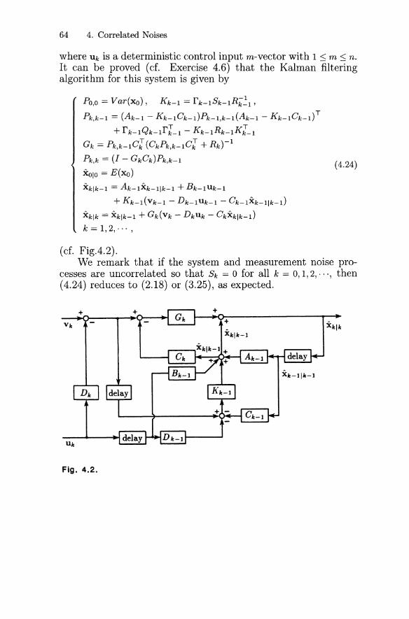
64 4. Correlated Noises
where Uk is a deterministic control input m-vector with 1 :::; m :::; n.It can be proved (cf. Exercise 4.6) that the Kalman filteringalgorithm for this system is given by
PO,O == Var(xo), Kk-l = rk-ISk-IRk~I'
Pk,k-l == (Ak- l - K k- l Ck-I)Pk-l,k-1 (Ak- l - Kk-lCk-l) T
+ rk-IQk-Irr-1 - Kk-IRk-IKJ_I
Gk = Pk,k-ICJ (CkPk,k-ICJ + Rk)-l
Pk,k == (1 - GkCk)Pk,k-1
xOlo == E(xo)
xklk-l == Ak-IXk-Ilk-1 + Bk-lUk-l
+ Kk-I(Vk-1 - Dk-IUk-1 - Ck-1Xk-Ilk-l)
xklk == xklk-l + Gk(Vk - DkUk - CkXk1k-l)
k = 1,2,," ,
(4.24)
(cf. Fig.4.2).We remark that if the system and measurement noise pro
cesses are uncorrelated so that Sk == 0 for all k == 0,1,2, . ", then(4.24) reduces to (2.18) or (3.25), as expected.
Fig. 4.2.
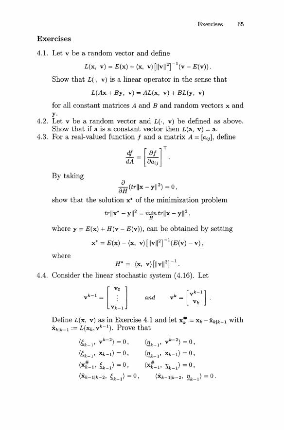
Exercises 65
Exercises
4.1. Let v be a random vector and define
L(x, v) = E(x) + (x, v) [llv I1 2]-l(v - E(v)) .
Show that L(·, v) is a linear operator in the sense that
L(Ax + By, v) = AL(x, v) + BL(y, v)
for all constant matrices A and B and random vectors x andy.
4.2. Let v be a random vector and L(·, v) be defined as above.Show that if a is a constant vector then L(a, v) == a.
4.3. For a real-valued function f and a matrix A = [aij], define
:~ = [:~j]T.By taking
8 28H (trllx - yll ) = 0,
show that the solution x* of the minimization problem
trllx* - yl12 = min trllx _ yl12 ,H
where y == E(x) + H(v - E(v)), can be obtained by setting
x* == E(x) - (x, v) [llv l1 2J-1 (E(v) - v) ,
whereH* = (x, v) [lI v Il 2] -1 .
4.4. Consider the linear stochastic system (4.16). Let
k-1 _ [ ~o ]v - .
Vk-1
and
Define L(x, v) as in Exercise 4.1 and let xt == Xk -xklk-l withxklk-l :== L(Xk,Vk - 1). Prove that
( k-2)~k_1'V =0,
(~k-l' Xk-l) == 0,
(Xt-l' ~k-l) == 0,
(Xk-llk-2, ~k-l) == 0,
(!1k-l' Vk
-2
) == 0,
(!lk-l' Xk-l) == 0,
(Xt-l' !lk-1) == 0,
(Xk-1Ik-2, !lk-l) == 0 .
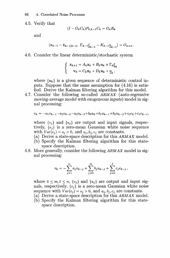
66 4. Correlated Noise Processes
4.5. Verify that
and
4.6. Consider the linear deterministic/stochastic system
{Xk+l = AkXk + BkUk + rk~k
Vk = CkXk + DkUk + '!1.k '
where {Uk} is a given sequence of deterministic control inputs. Suppose that the same assumption for (4.16) is satisfied. Derive the Kalman filtering algorithm for this model.
4.7. Consider the following so-called ARMAX (auto-regressivemoving-average model with exogeneous inputs) model in signal processing:
where {Vj} and {Uj} are output and input signals, respectively, {ej} is a zero-mean Gaussian white noise sequencewith V ar(ej) == Sj > 0, and aj, bj , Cj are constants.(a) Derive a state-space description for this ARMAX model.(b) Specify the Kalman filtering algorithm for this state-
space description.4.8. More generally, consider the following ARMAX model in sig
nal processing:
n m l
Vk == - L ajVk-j +L bjUk-j + L Cjek-j ,
j=l j=O j=O
where 0 ~ rn, R ~ n, {Vj} and {Uj} are output and input signals, respectively, {ej} is a zero-mean Gaussian white noisesequence with V ar(ej) == Sj > 0, and aj, bj , Cj are constants.(a) Derive a state-space description for this ARMAX model.(b) Specify the Kalman filtering algorithm for this state-
space description.
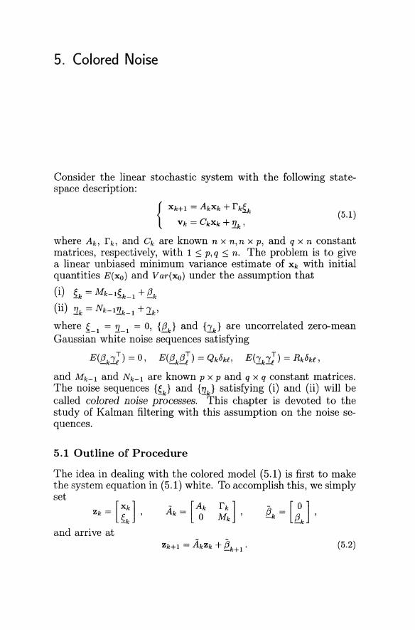
5. Colored Noise
Consider the linear stochastic system with the following statespace description:
{
Xk+l = AkXk + rk~k(5.1)
Vk = CkXk + '!lk '
where Ak, rk, and Ck are known n x n, n x p, and q x n constantmatrices, respectively, with 1 :::; p, q :::; n. The problem is to givea linear unbiased minimum variance estimate of Xk with initialquantities E(xo) and Var(xo) under the assumption that
(i) ~k = Mk-l~k_l + f!.-k
(ii) '!lk = Nk-l'!lk_l + lk'
where ~-l = '!l-l = 0, {~k} and {lk} are uncorrelated zero-meanGaussian white noise sequences satisfying
E(f!.-kL) = 0, E(f!.-ktJ) = Qk8ki, E(1.kl.£T) = Rk8ki ,
and Mk-l and Nk-l are known p x p and q x q constant matrices.The noise sequences {~k} and {'!lk} satisfying (i) and (ii) will becalled colored noise processes. This chapter is devoted to thestudy of Kalman filtering with this assumption on the noise sequences.
5.1 Outline of Procedure
The idea in dealing with the colored model (5.1) is first to makethe system equation in (5.1) white. To accomplish this, we simplyset
Zk = [{:] ,
and arrive at(5.2)
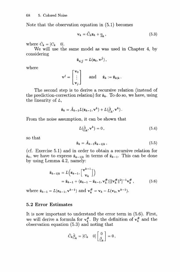
68 5. Colored Noise
Note that the observation equation in (5.1) becomes
(5.3)
where Ok = [Ck 0].We will use the same model as was used in Chapter 4, by
considering
where
The second step is to derive a recursive relation (instead ofthe prediction-correction relation) for Zk. To do so, we have, usingthe linearity of L,
,,- k - kZk = Ak-1L(Zk-l, V ) + L(f!.k' V ).
From the noise assumption, it can be shown that
- kL(!!.k' V ) = 0 ,
so that
(5.4)
(5.5)
(cf. Exercise 5.1) and in order to obtain a recursive relation forZk, we have to express Zk-llk in terms of Zk-l. This can be doneby using Lemma 4.2, namely:
5.2 Error Estimates
It is now important to understand the error term in (5.6). First,we will derive a formula for vt. By the definition of vt and theobservation equation (5.3) and noting that
(\~k = [Ck oJ [;J = 0,
5.2 Error Estimates 69
we have
Vk = CkZk + '!lk
= CZk + Nk-1'!lk_1 + lk
= Ck(Ak-1Zk- 1 + ~k) + Nk-1(Vk-1 - Ck-1Zk-1) + lk
= Hk-1Zk-1 + Nk-1Vk-1 + lk ' (5.7)
withHk-1 = ckAk- 1 - Nk-1Ck-1
= [CkAk-1 - Nk-1Ck-1 Ckfk-1].
Hence, by the linearity of L, it follows that
L(Vk, v k - 1)
=Hk-1L(Zk-1, v k-
1) + Nk-1L(Vk-1, v k
-1
) + L(lk' v k-
1).
S· ( k-1) '"Ince L Zk-1, v = Zk-1,
(5.8)
(cf. Exercise 5.2), and
we obtain# L( k-1)Vk=Vk- Vk,V
= Vk - (Hk-1Zk-1 + Nk-1Vk-1)
= Vk - Nk-1Vk-1 - Hk-1Zk-1 .
In addition, by using (5.7) and (5.10), we also have
(5.9)
(5.10)
(5.11)
Now, let us return to (5.6). Using (5.11), (5.10), and (Zk-1
zk-1,lk) = 0 (cf. Exercise 5.3), we arrive at
Zk-1lk
_ '" ( '" #)[11 #11 2]-1 #- Zk-1 + Zk-1 - Zk-1, V k V k V k
= Zk-1 + Ilzk-1 - zk_1112 H,J-1(Hk-1Ilzk-1 - Zk_111
2 H;-l + Rk)-l
. (Vk - Nk-1Vk-1 - Hk-1Zk-1).
Putting this into (5.5) gives
70 5. Colored Noise
or
[1:] = [A~-l ft:~lJ [1:=:]+ Gk (Vk - Nk-lVk-l - Hk-l [1:=:]) , (5.12)
where
with(5.14)
(5.15)
5.3 Kalman Filtering Process
What is left is to derive an algorithm to compute Pk and theinitial condition zoo Using (5.7), we have
= (Ak-1Zk-l + ~k) - (Ak-1Zk- 1 + Gk(Vk - Nk-lVk-l - Hk-izk-l))
= Ak-l(Zk-l - Zk-l) + ~k - Gk(Hk-lZk-l + lk - Hk-lZk-l)
= (Ak- 1 - GkHk-l)(Zk-l - Zk-l) + (~k - Gklk) .
In addition, it follows from Exercise 5.3 and (Zk-l - Zk-l, ~k) = 0
(cf. Exercise 5.4) that- - T
Pk = (Ak- 1 - GkHk-l)Pk-l(Ak- 1 - GkHk-l)
+ [~ ~k] + GkRkGr
- - [0 0]= (Ak- 1 - GkHk-l)Pk-lAk-l + 0 Qk '
where the identity- T T
- (Ak- 1 - GkHk-l)Pk-l(GkHk-l) + GkRkG k
= - Ak-1Pk-lH"[_lGl + GkHk-lPk-lH"[_lGl + GkRkGl
= - Ak-1Pk-lH"[_1Gl + Gk(Hk-lPk-lH"[_l + Rk)Gl- T T - T T
== - Ak-lPk-lHk-lGk + Ak-lPk-lHk-lGk
==0,
which is a consequence of (5.13), has been used.

5.3 Kalman Filtering Process 71
The initial estimate is
Zo = L(zo, vo) = E(zo) - (zo, vo)[Il vo\l2]-1(E(vo) - vo)
= [E~o)] _ [Var(i)Cl] [CoVar(Xo)CJ + Rot l
. (CoE(xo) - vo) . (5.16)
We remark that
and since
Zk - Zk
= (Ak- 1 - Gk Hk-l)(Zk-1 - Zk-1) + (§.k - Gk]k)
= (Ak- 1 - GkHk-l) ... (Ao - G1Ho)(zo - Zo) + noise,
we have E(Zk - Zk) = o. That is, Zk is an unbiased linear minimum(error) variance estimate of Zk.
In addition, from (5.16) we also have the initial condition
Po =Var(zo - zo)
=Var([Xo - E(xo)]~o
[ V ar (xo)cl ] [ () T ] -1 [ () ])+ 0 CoVar Xo Co + Ro CoE Xo - Vo
[
Var(xo - E(xo) 0 ]= +var(xo)CJ[Covar(xo):J + ~J-l[CoE(xo) - Vo]) Qo
[
Var(xo) 0 ]__ -[var(xo)]Cl[covar(Xoo)C;J + Ro]-lCo[Var(xo)] ( )5.17a
Qo
(cf. Exercise 5.5). If Var(xo) is nonsingular, then using the matrixinversion lemma (cf. Lemma 1.2), we have
(5.17b)
72 5. Colored Noise
Finally, returning to the definition Zk = [~~], we have
Zk == L(Zk, v k)
== E(Zk) + (Zk, vk)[llvkI12]-1(vk - E(vk))
== [E (Xk)] + [(Xk, v:) ] [11 vk 11 2] -1 (vk _ E (vk ) )E({k) ({k'V )
_ [E(Xk) + (Xk, vk)[llvkI12]-1(vk - E(vk))]- E(~) + (~ ,vk)[llvkI12]-1(vk - E(vk))
-k -k
=[1:] .In summary, the Kalman filtering process for the colored
noise model (5.1) is given by
[ ~k] ==[Ak-1 f k- 1 ] [~k-1]fk 0 Mk-1 fk-1
+ Gk ( Vk - Nk-lVk-l - Hk-l [1:=~]) , (5.18)
where
and
(5.19)G [ Ak-1 f k - 1 ] D HT (H D HT R )-1k == 0 Mk-1 rk-1 k-1 k-1rk-1 k-1 + k
with Pk-1 given by the formula
([ Ak- 1 f k - 1 ] ) [Al- 1 0]Pk = 0 Mk-l - GkHk-l Pk-l rLl MLI
+ [~ ~J, (5.20)
The initial conditions are given by (5.16) and (5.17ak == 1,2,···.or 5.17b).
We remark that if the colored noise processes become white(that is, both Mk == 0 and Nk == 0 for all k), then this Kalmanfiltering algorithm reduces to the one derived in Chapters 2 and3, by simply setting
xklk-1 == Ak-1Xk-1Ik-1 ,so that the recursive relation for Xk is decoupled into two equations: the prediction and correction equations. In addition, bydefining Pk == Pk1k and
Pk,k-1 == Ak-1Pk-1Al-1 + fkQkfl ,
it can be shown that (5.20) reduces to the algorithm for computing the matrices Pk,k-1 and Pk,k. We leave the verification as anexercise to the reader (cf. Exercise 5.6).
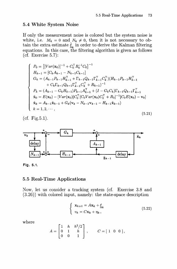
5.5 Real-Time Applications 73
5.4 White System Noise
If only the measurement noise is colored but the system noise iswhite, i.e. Mk = 0 and Nk =1= 0, then it is not necessary to obtain the extra estimate ~k in order to derive the Kalman filteringequations. In this case, the filtering algorithm is given as follows(cf. Exercise 5.7) :
Po = [[Var(xo)]-l + C~Ra1Co]-1
Hk-1 = [CkAk-1 - Nk-1Ck-1]
Gk = (Ak-1Pk-1H"[_1 + rk-1Qk-lrl-lC"[)(Hk-1Pk-lH"[-1
+ Ckrk-1Qk-lrl_1C"[ + Rk_l)-l
Pk = (Ak- 1 - GkHk-1)Pk-lAl-l + (1 - GkCk)rk-1Qk-1rl_l
Xo = E(xo) - [Var(xo)]C~[CoVar(xo)C~ + RO]-l[CoE(xo) - Vo]
Xk = Ak-lXk-l + Gk(Vk - Nk-lVk-l - Hk-lXk-l)
k = 1,2,··· ,(5.21)
(cf. Fig.5.!).
+
Fig. 5.1.
5.5 Real-Time Applications
Now, let us consider a tracking system (cf. Exercise 3.8 and(3.26)) with colored input, namely: the state-space description
where
{
Xk+l = AXk + 5.k
Vk = CXk + TJk ,(5.22)
C=[1 00],
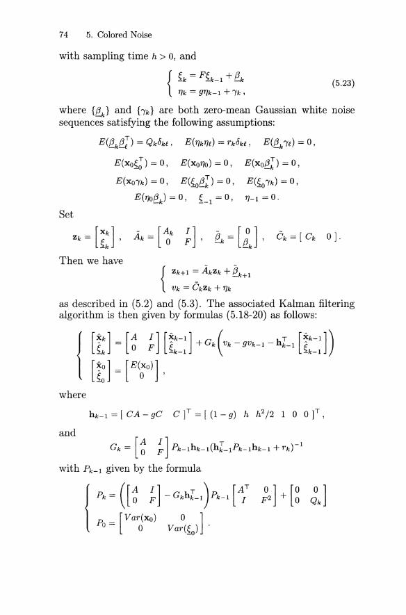
74 5. Colored Noise
with sampling time h > 0, and
{~k = F~k_1 + f!..k
(5.23)'TJk = g'TJk-1 +Ik,
where {~k} and {Ik} are both zero-mean Gaussian white noisesequences satisfying the following assumptions:
E(~kri:) = Qkbkl, E(1]k1]l) = rkbkl , E(~kIl) = 0,
E(xo~~) = 0, E(xo'TJo) = 0, E(xo~~) = 0,
E(XOlk) = 0, E(~o~~) = 0, E(~oIk) = 0,
E(1]o{ik) = 0, ~-1 = 0, 1]-1 = o.Set
Zk = [{:] ,
Then we have
~k = [;J '{
Zk+1 = Akzk + ~k+1
Vk = CkZk + 1]k
as described in (5.2) and (5.3). The associated Kalman filteringalgorithm is then given by formulas (5.18-20) as follows:
where
hk-1 == [ CA - gC C]T = [ (1 - g) h h 2 /2 1 0 O]T,
and
[AI] ( T )-1Gk == 0 F Pk-1hk-1 hk- 1Pk-1 hk-1 + rk
with Pk-1 given by the formula
o"] [0 0]p2 + 0 Qk
Exercises 75
Exercises
5.1. Let {~k} be a sequence of zero-mean Gaussian white noiseand {Vk} a sequence of observation data as in the system(5.1). Set
and define L(x, v) as in (4.6). Show that
- kL(~k' V ) = o.
5.2. Let {Ik} be a sequence of zero-mean Gaussian white noiseand v k and L(x, v) be defined as above. Show that
andL(Ik,Vk- 1
) = o.
5.3. Let {Ik} be a sequence of zero-mean Gaussian white noiseand v k and L(x, v) be defined as in Exercise 5.1. Furthermore, set
" L( k-l)Zk-l = Zk-l, V
Show that
and[
X k - 1 ]Zk-l = ~ .
-k-l
(Zk-l - Zk-l, Ik) = o.
5.4. Let {~k} be a sequence of zero-mean Gaussian white noiseand set
Furthermore, define Zk-l as in Exercise 5.3. Show that
5.5. Let L(x, v) be defined as in (4.6) and set Zo = L(zo, vo) with
zo=[~].
76 5. Colored Noise
Show that
Var(zo - zo)
[
Var(xo)= -[Var(xo)]cJ[CoVar(x~CJ +.Ro]-lCo[Var(xo)]
5.6. Verify that if the matrices Mk and Nk defined in (5.1) areidentically zero for all k, then the Kalman filtering algorithmgiven by (5.18-20) reduces to the one derived in Chapters2 and 3 for the linear stochastic system with uncorrelatedsystem and measurement white noise processes.
5.7. Simplify the Kalman filtering algorithm for the system (5.1)where Mk == 0 but Nk =1= o.
5.8. Consider the tracking system (5.22) with colored input(5.23) .(a) Reformulate this system with colored input as a new
augmented system with Gaussian white input by setting
Ac == [~ ~ ~] and Cc == [C 0 0 0 1].o 0 9
(b) By formally applying formulas (3.25) to this augmentedsystem, give the Kalman filtering algorithm to the tracking system (5.22) with colored input (5.23).
(c) What are the major disadvantages of this approach ?
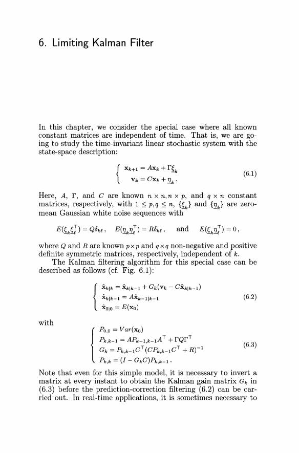
6. Limiting Kalman Filter
In this chapter, we consider the special case where all knownconstant matrices are independent of time. That is, we are going to study the time-invariant linear stochastic system with thestate-space description:
{Xk+l: AXk + r{k
Vk - CXk +'!1k'(6.1)
Here, A, r, and C are known n x n, n x p, and q x n constantmatrices, respectively, with 1 ~ p, q ~ n, {~k} and {'!1k} are zeromean Gaussian white noise sequences with
where Q and R are known pxp and q x q non-negative and positivedefinite symmetric matrices, respectively, independent of k.
The Kalman filtering algorithm for this special case can bedescribed as follows (cf. Fig. 6.1):
with
{
~klk = Xklk~l + Gk(Vk - CXklk-l)
Xklk-l = AXk-llk-l
:Kolo = E(xo)
(6.2)
(6.3)
Po,o = Var(xo)
Pk,k-l = APk_l,k_lAT + rQrT
Gk = Pk,k_lCT (CPk,k_l CT + R)-l
Pk,k = (I - GkC)Pk,k-l .
Note that even for this simple model, it is necessary to invert amatrix at every instant to obtain the Kalman gain matrix Gk in(6.3) before the prediction-correction filtering (6.2) can be carried out. In real-time applications, it is sometimes necessary to
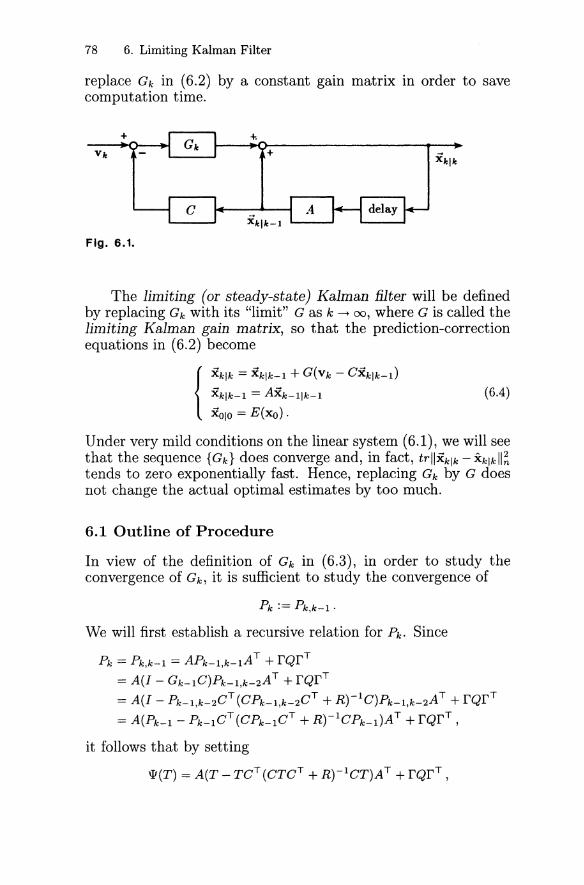
78 6. Limiting Kalman Filter
replace Gk in (6.2) by a constant gain matrix in order to savecomputation time.
++
(6.4)
Fig. 6.1.
The limiting (or steady-state) Kalman filter will be definedby replacing G k with its "limit" G as k --4 00, where G is called thelimiting Kalman gain matrix, so that the prediction-correctionequations in (6.2) become
{
~klk = Xklk~l + G(Vk - CXklk-l)
Xklk-l = AXk-llk-l
xala = E(xo) .
Under very mild conditions on the linear system (6.1), we will seethat the sequence {Gk} does converge and, in fact, trllxklk - xklk 11;tends to zero exponentially fast. Hence, replacing Gk by G doesnot change the actual optimal estimates by too much.
6.1 Outline of Procedure
In view of the definition of Gk in (6.3), in order to study theconvergence of Gk, it is sufficient to study the convergence of
Pk := Pk,k-l .
We will first establish a recursive relation for Pk. Since
Pk = Pk,k-l == APk-l,k-lAT + rQrT
= A(I - Gk-l C )Pk-l,k-2AT +rQrT
= A(I - Pk-l,k-2CT (CPk-l,k-2CT + R)-lC)Pk_l,k_2AT + rQrT
== A(Pk- 1 - Pk_lCT (CPk_l CT + R)-lCPk_1)AT + rQrT,
it follows that by setting
'lJ(T) = A(T - TCT (CTCT + R)-lCT)AT + rQrT,
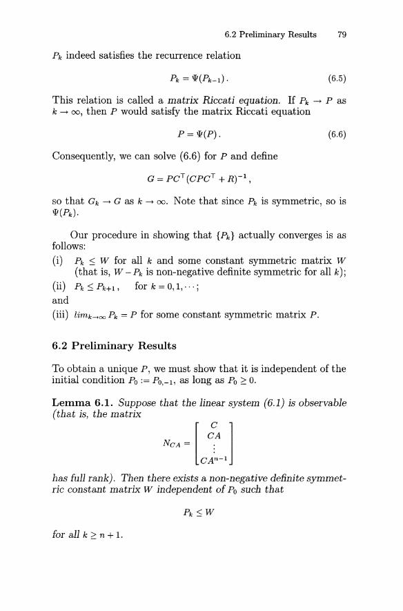
6.2 Preliminary Results 79
Pk indeed satisfies the recurrence relation
(6.5)
This relation is called a matrix Riccati equation. If Pk ~ P ask ~ 00, then P would satisfy the matrix Riccati equation
P = 'I!(P) .
Consequently, we can solve (6.6) for P and define
G = PCT (CPCT + R)-l,
(6.6)
so that Gk ~ G as k ~ 00. Note that since Pk is symmetric, so is'I!(Pk).
Our procedure in showing that {Pk} actually converges is asfollows:(i) Pk:S W for all k and some constant symmetric matrix W
(that is, W -Pk is non-negative definite symmetric for all k);
(ii) Pk:S Pk+l, for k = 0,1,···;
and(iii) limk-+oo Pk = P for some constant symmetric matrix P.
6.2 Preliminary Results
To obtain a unique P, we must show that it is independent of theinitial condition Po := PO,-l, as long as Po 2:: o.
Lemma 6.1. Suppose tbat tbe linear system (6.1) is observable(tbat is, the matrix
[
C ]CANCA = .
CA·n-l
has full rank). Tben tbere exists a non-negative definite symmetric constant matrix W independent of Po sucb tbat
for all k 2:: n + 1.
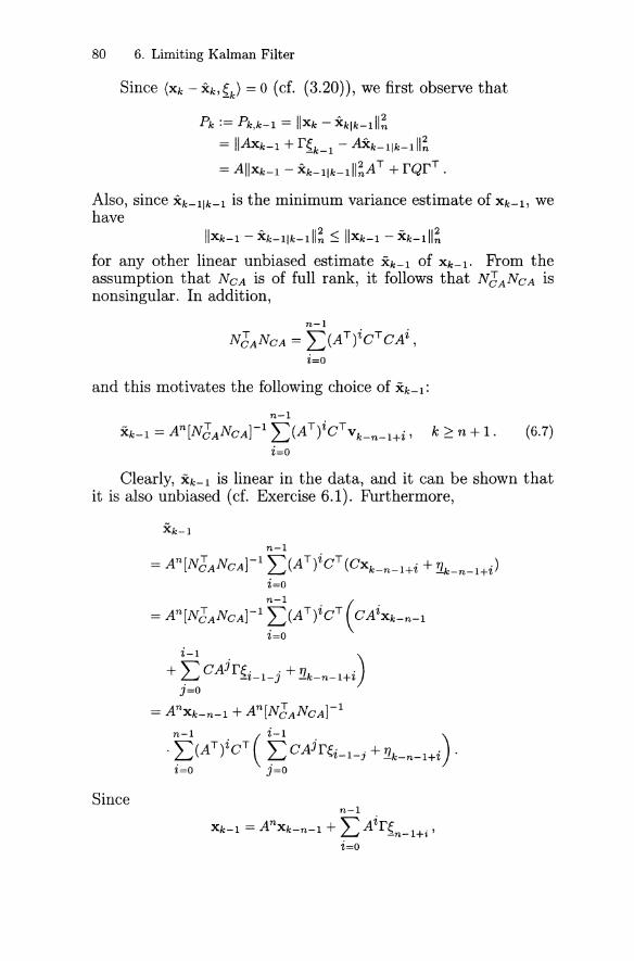
80 6. Limiting Kalman Filter
Since (Xk - Xk,S-k) = 0 (cf. (3.20)), we first observe that
Pk := Pk,k-l = II x k - xklk-lll~
= IIAxk-l + r{k_l - AXk-llk-lll~
= Allxk-l - Xk_llk_lll~AT + rQrT .
Also, since Xk-llk-l is the minimum variance estimate of Xk-l, wehave
Ilxk-l - Xk-llk-lll~ ::; II x k-l - xk-lll~
for any other linear unbiased estimate Xk-l of Xk-l. From theassumption that NCA is of full rank, it follows that NJANCA isnonsingular. In addition,
n-lNJANCA = L(AT)iCTCAi ,
i=o
and this motivates the following choice of Xk-l:
n-lXk-l = An[NJANcA]-l L(AT)iCTVk-n-1+i, k 2: n + 1. (6.7)
i=o
Clearly, Xk-l is linear in the data, and it can be shown thatit is also unbiased (cf. Exercise 6.1). Furthermore,
n-l
= An [N6ANcAt 1 L(AT)iCT(Cxk-n-l+i + !l.k-n-l+i)
i=o
Sincen-l
Xk-l = AnXk_n_l + L Air{n_l+i 'i=o
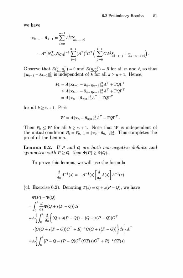
6.2 Preliminary Results 81
we have
n-I
Xk-I - Xk-I = '" Air~ I,jL.-t -n- +lJi=o
n-I i-I
- An [N6A NCAr1
L(AT)iCT ( L CAj~i-l-j +!Ik-n-l+i) .i=o j=o
Observe that E(5..m !JJ) = 0 and E(?1!JJ) = R for all m and £, so thatIlxk-1 - Xk-Ill; is independent of k for all k ~ n + 1. Hence,
Pk = Allxk-I - Xk_Ilk_III;AT + rQrT
~ Allxk-I - Xk_Ilk_III;AT + rQrT
= Allxn- xnlnll~AT + rQrT
for all k ~ n + 1. Pick
W = Allxn- xnlnll;AT+ rQrT.
Then Pk ~ W for all k ~ n + 1. Note that W is independent ofthe initial condition Po = PO,-I = IIxo -xo,-Ill;. This completes theproof of the Lemma.
Lemma 6.2. If P and Q are both non-negative definite andsymmetric with P ~ Q, then \l1(P) ~ \l1(Q).
To prove this lemma, we will use the formula
:SA-1(s) = -A-1(s) [:sA(S)]A-1(s)
(cf. Exercise 6.2). Denoting T(s) = Q + s(P - Q), we have
\l1(P) - \l1(Q){I d
= la ds iJ!(Q + s(P - Q»ds
=A{11
:s {(Q + s(P - Q» - (Q + s(P - Q»CT
. [C(Q + s(P - Q»CT + Rr1C(Q + s(P - Q» }dS }AT
=A{11
[P - Q - (P - Q)CT (CT(s)CT + R)-lCT(s)
82 6. Limiting Kalman Filter
- T(s)CT (CT(s)CT + R)-IC(p - Q) + T(s)CT (CT(s)CT + R)-l
. C(P - Q)CT (CT(s)CT + R)-lCT(s)]ds }AT
=A{11
[T(s)CT (CT(s)CT + R)-lC](p - Q)
. [T(s)CT (CT(s)CT + R)-lC]TdS}A
20.
Hence, \lJ(P) 2 \lJ(Q) as required.
We also have the following:
Lemma 6.3. Suppose that the linear system (6.1) is observable.Then with the initial condition Po = PO,-l = 0, the sequence {Pk}converges componentwise to some symmetric matrix P 2 0 ask -t 00.
SincePI := IIXI - xlloll; 20= Po
and both Po and PI are symmetric, Lemma 6.2 yields
Pk+l 2 Pk , k = 0, 1, ....
Hence, {Pk} is monotonic nondecreasing and bounded above byw (cf. Lemma 6.1). For any n-vector y, we have
o ::; yT PkY ::; YTWy,
so that the sequence {yT PkY} is a bounded non-negative monotonic nondecreasing sequence of real numbers and must convergeto some non-negative real number. If we choose
y = [0···0 1 0·· .O]T
with 1 being placed at the ith component, then setting Pk = [p~~)],
we haveTp (k) k
Y kY = Pii ----t Pii as ----t 00
for some non-negative number Pii. Next, if we choose
Y = [0···0 1 0···0 1 0·· .O]T
6.2 Preliminary Results 83
with the two 1's being placed at the ith and jth components,then we have
YT PkY =P~~) + p~~) + p(,~) + p(~~~~ ~J J~ JJ
=P~~) + 2p~~) + p(.k~ -+ q as k -+ 00~~ ~J JJ
for some non-negative number q. Since p~~) -+ Pii' we have
That is, Pk -+ P. Since Pk 2: 0 and is symmetric, so is P. Thiscompletes the proof of the lemma.
We now defineG = lim Gk,
k~(X)
where Gk = PkCT (CPkCT + R)-l. Then
G = PCT (CPCT + R)-l. (6.8)
Next, we will show that for any non-negative definite symmetricmatrix Po as an initial choice, {Pk} still converges to the sameP. Hence, from now on, we will use an arbitrary non-negativedefinite symmetric matrix Po, and recall that Pk = '1J(Pk-l) , k =1,2, ... , and P = '1J(P). We first need the following.
Lemma 6.4. Let tbe linear system (6.1) be observable so tbatP can be defined using Lemma 6.3. Tben tbe following relation
bolds for all k = 1,2" ", and any non-negative definite symmetricinitial condition Po.
Since Gk-l = Pk_lCT (CPk_l CT + R)-l and P;:-l = Pk-l, thematrix Gk-lCPk-l is non-negative definite and symmetric, so thatGk-lCPk-l = Pk-lCTGl_l' Hence, using (6.5) and (6.6), we have
P-Pk
= '1J(P) - '1J(Pk-l)
= (APAT - AGCPAT ) - (APk_lAT - AGk-lCPk_lAT)
= APAT - AGCPAT - APk_lAT + APk_1CTGl_1AT . (6.10)
84 6. Limiting Kalman Filter
Now,
(I - GC)(P - Pk-l)(1 - Gk_lC)T
=P - Pk-l + Pk_1CTGl- 1 - GCP + Re, (6.11)
where
Re = GCPk-l - PCTGl-1 + GCPCTGl-1 - GCPk_lCTGl-1 . (6.12)
Hence, if we can show that Re = 0, then (6.9) follows from (6.10)and (6.11). From the definition of Gk-l, we have Gk_l(CPk_lCT +R) = Pk_lCT or (CPk_lCT + R)Gk-l = CPk-l, so that
Gk-lCPk-lCT = Pk_lCT - Gk-lR (6.13)
orCPk_l CT Gl- 1 = CPk-l - RGl-1 . (6.14)
Taking k ~ 00 in (6.13) with initial condition Po := PO,-l = 0, wehave
GCPCT = PCT - GR, (6.15)
and putting (6.14) and (6.15) into (6.12), we can indeed concludethat Re = 0. This completes the proof of the lemma.
Lemma 6.5.
Pk =[A(I - Gk-lC)]Pk-l[A(I - Gk_lC)]T
+ [AGk_l]R[AGk_l]T + rQrT (6.16)
and consequently, for an observable system with Po := PO,-l = 0,
P = [A(I - GC)]P[A(I - GC)]T + [AG]R[AG]T +rQrT. (6.17)
Since Gk_l(CPk_lCT + R) = Pk_lCT from the definition, wehave
and hence,
AGk-lRGl_lAT = A(I - Gk-lC)Pk-lCTGl_1AT .
Therefore, from the matrix Riccati equation Pk = W(Pk-l), we mayconclude that
Pk = A(1 - Gk_lC)Pk_l AT + rQrT
= A(I - Gk-lC)Pk-l(I - Gk_lC)T AT
+ A(I - Gk-lC)Pk-lCTGl_1AT + rQrT
= A(I - Gk-lC)Pk-l(I - Gk_lC)T AT
+ AGk-1RGl_1AT +rQrT
which is (6.16).
6.2 Preliminary Results 85
Lemma 6.6. Let the linear system (6.1) be (completely) controllable (that is, the matrix
has full rank). Then for any non-negative definite symmetricinitial matrix Po, we have Pk > 0 for k ~ n + 1. Consequently,P >0.
Using (6.16) k times, we first have
Pk = fQfT + [A(I - Gk_IC)]fQfT[A(I - Gk_IC)]T + ... + {[A(I-
Gk-IC)]", [A(I - G2C)]}fQfT{[A(I - Gk-IC)],,· [A(I - G2C)]}T
+ [AGk_I]R[AGk_I]T + [A(I - Gk-IC)][AGk-2]R[AGk-2]T
. [A(I - Gk_IC)]T + ... + {[A(I - Gk-IC)]
... [A(I - G2C)][AGI ]}R{[A(I - Gk-IC)]
... [A(I - G2C)][AGI ]} T + {[A(I - GkC)]
... [A(I - GIC)]}Po{[A(I - GkC)] ... [A(I - GIC)]}T .
To prove that Pk > 0 for k ~ n + 1, it is sufficient to show thatYT PkY = 0 implies Y = o. Let·y be any n-vector such that YT PkY =o. Then, since Q, R and Po are non-negative definite, each termon the right hand side of the above identity must be zero. Hence,we have
YTfQfTY = 0, (6.18)
y T[A(I - Gk_IC)]fQfT[A(I - Gk_IC)]TY = 0, (6.19)
YT{[A(I - Gk-IC)],,· [A(I - G2C)]}fQfT
. {[A(I - Gk-IC)]", [A(I - G2C)]}T Y = 0 (6.20)
and
YT {[A(I - Gk-IC)]·" [A(I - G3C)] [AG2]}R
. {[A(I - Gk-IC)]", [A(I - G3C)][AG2]}Ty = o. (6.22)
Since R > 0, from (6.21) and (6.22), we have
yT AGk-1 = 0, (6.23)
86 6. Limiting Kalman Filter
yT[A(l - Gk-lC )]··· [A(l - G2C)][AG1] = o. (6.24)
Now, it follows from Q > 0 and (6.18) that
and then using (6.19) and (6.23) we obtain
yTAr=o,
and so on. Finally, we have
YT Ajr = 0, j = 0,1,·· . ,n - 1 ,
as long as k 2: n + 1. That is,
yTMAry=yT[r Ar ... An-1r]y=0.
Since the system is (completely) controllable, MAr is of full rank,and we must have y = o. Hence, Pk > 0 for all k 2: n + 1. Thiscompletes the proof of the lemma.
Now, using (6.9) repeatedly, we have
P - Pk = [A(l - Gc)]k-n-l(p - Pn+1)BJ , (6.25)
where
Bk = [A(l - Gk-lC)]··· [A(l - Gn+1C)] , k = n + 2, n + 3,··· ,
with Bn+1 := I. In order to show that Pk ~ P as k ~ 00, it issufficient to show that [A(l - Gc)]k-n-l ~ 0 as k ~ 00 and Bk is"bounded." In this respect, we have the following two lemmas.
Lemma 6.7. Let the linear system (6.1) be observable. Then
for some constant matrix M. Consequently, if Bk = [b~j)] then
I(k)1bij :Srn,
for some constant rn and for all i,j and k.
6.2 Preliminary Results 87
By Lemma 6.1, Pk ~ W for k ~ n + 1. Hence, using Lemma6.5 repeatedly, we have
W ~ Pk ~ [A(1 - Gk-lC)]Pk-l[A(1 - Gk_lC)]T
~ [A(1 - Gk-lC)][A(1 - Gk-2C)]Pk-2
. [A(1 - Gk_2C)]T[A(1 - Gk_1C)]T
Since Pn +1 is real, symmetric, and positive definite, by Lemma6.6, all its eigenvalues are real, and in fact, positive. Let Amin bethe smallest eigenvalue of Pn+1 and note that Pn+1 ~ Amin1 (cf.Exercise 6.3). Then we have
Setting M = A~~nW completes the proof of the lemma.
Lemma 6.8. Let A be an arbitrary eigenvalue of A(1 - GC). Ifthe system (6.1) is both (completely) controllable and observable,then IAI < 1.
Observe that A is also an eigenvalue of (I - GC)T AT. Let y bea corresponding eigenvector. Then
(6.26)
Using (6.17), we have
yTPy = "XyTPAy + yT[AG]R[AG]TY+ yTrQrTy.
Hence,(1 - IAI 2 )yTPy = YT [(AG)R(AG) T + rQrT]y .
Since the right-hand side is non-negative and yTPy ~ 0, we musthave 1 -IAI 2 ~ 0 or IAI ~ 1. Suppose that IAI = 1. Then
51T (AG)R(AG) T Y = 0~----::~T T
or [(AG)T y ] R[(AG) y] = 0
andyTrQrTy = 0 or
Since Q > 0 and R > 0, we have
GTATy=O (6.27)
88 6. Limiting Kalman Filter
andr T y = 0,
so that (6.26) implies ATy = AY. Hence,
rT(Aj)TY=AjrTy=o, j=0,1,···,n-1.
This givesyTMAr=yT[r Ar ... An-1r] =0.
Taking real and imaginary parts, we have
[Re(y)]T MAr = 0 and [Im(y)]T MAr = o.
(6.28)
Since y =1= 0, at least one of Re(y) and Im(y) is not zero. Hence,MAr is row dependent, contradicting the complete controllabilityhypothesis. Hence IAI < 1. This completes the proof of the lemma.
6.3 Geometric Convergence
Combining the above results, we now have the following.
Theorem 6.1. Let the linear stochastic system (6.1) be both(completely) controllable and observable. Then, for any initialstate Xo such that Po := PO,-l = Var(xo) is non-negative definiteand symmetric, Pk := Pk,k-l ~ P as k ~ 00, where P > 0 is symmetric and is independent of xo. Furthermore, the order of convergence is geometric; that is,
(6.29)
where 0 < r < 1 and C > 0, independent of k. Consequently,
(6.30)
To prove the theorem, let p = A(I - GC). Using Lemma 6.7and (6.25), we have
(Pk - P)(Pk - P) T
=pk-n-l(Pn+1 - P)BkBJ (Pn+1 - p)(pk-n-l)T
5:pk-n-1o(pk-n-l) T
for some non-negative definite symmetric constant matrix o.From Lemma 6.8, all eigenvalues of p are of absolute value less
6.3 Geometric Convergence 89
than 1. Hence, F k ~ 0 so that Pk ~ P as k ~ 00 (cf. Exercise6.4). On the other hand, by Lemma 6.6, P is positive definitesymmetric and is independent of Po.
Using Lemmas 1.7 and 1.10, we havetr(Pk - P)(Pk - p)T :::; trFk-n-l(Fk-n-l)T . trO:::; Crk ,
where 0 < r < 1 and C is independent of k. To prove (6.30), wefirst rewrite
Gk -G
= PkCT (CPk CT + R)-l - PCT (CPCT + R)-l
= (Pk - P)CT (CPk CT + R)-l
+ PCT[(CPkCT + R)-l - (CPCT + R)-l]
= (Pk - P)CT (CPk CT + R)-l + PCT (CPk CT + R)-l
. [(CPCT + R) - (CPk CT + R)](CPCT + R)-l
= (Pk - P)CT (CPk CT + R)-l
+ PCT (CPkCT + R)-lC(p - Pk)CT (CPCT + R)-l.
Since for any n x n matrices A and B,
(A+B)(A+B)T :::;2(AAT +BBT )
(cf. Exercise 6.5), we have
(Gk - G) (Gk - G) T
:::;2(Pk - P)CT (CPkCT + R)-l(CPkCT + R)-lC(Pk - P)
+ 2PCT (CPk CT + R)-lC(p - Pk)CT (CPCT + R)-l
. (CPCT + R)-lC(p - Pk)CT (CPk CT + R)-lCp. (6.31)
And since Po :::; Pk, we have CPocT + R :::; CPkCT + R, so that byLemma 1.3,
(CPk CT + R)-l :::; (CPoCT + R)-l ,
and hence, by Lemma 1.9,
tr(CPkCT + R)-l(CPkCT + R)-l :::; (tr(CPoCT + R)-1)2.
Finally, by Lemma 1.7, it follows from (6.31) that
tr (G k - G) (Gk - G) T
:::; 2tr(Pk - P)(Pk - p)T . trCTC(tr(CPoCT + R)-1)2
+ 2trppT . trCTC(tr(CPoCT + R)-1)2 . trCCT
. tr(P - Pk)(P - Pk)T . trCTC· tr(CPCT + R)-l(CPCT + R)-l
:::; Cl tr(Pk - P)(Pk - p)T
:::; Crk,
where Cl and C are constants, independent of k. This completesthe proof of the theorem.
90 6. Limiting Kalman Filter
The following result shows that Xk is an asymptotically optimal estimate of Xk.
Theorem 6.2. Let the linear system (6.1) be both (completely)controllable and observable. Then
lim Ilxk - xkll; = (p-l + c T R-1C)-1 = lim Ilxk - xkll; .k~~ k~~
The second equality can be easily verified. Indeed, usingLemma 1.2 (the matrix inversion lemma), we have
lim Ilxk - xkll;k~~
= lim Pk kk~~ ,
= lim (1 - GkC)Pk,k-lk~~
= (1 - GC)P
= P - PCT (CPCT + R)-lCp
= (P- 1 + c T R-1C)-1 > o.
Hence, to verify the first equality, it is equivalent to showing thatIlxk - xkll; -+ (1 -GC)P as k -+ 00. We first rewrite
Xk -Xk
= (AXk-l + fik _ 1) - (AXk-l + GVk - GCAXk-l)
= (AXk-l + fik_l) - AXk-l
- G(CAXk-l + Cfik_ 1 + ~k) + GCAXk-l
= (1 - GC)A(Xk-l - Xk-l) + (1 - GC)f~k_l - G~k . (6.32)
Since(6.33)
and(Xk-l - Xk-l' ~k) = 0 (6.34)
(cf. Exercise 6.6), we have
Ilxk - xkll;
=(1 - GC)Allxk-l - Xk_lll;AT (1 - GC)T
+ (1 - GC)fQfT (1 - GC)T + GRGT . (6.35)
On the other hand, it can be proved that
Pk,k =(1 - GkC)APk-l,k-lAT (1 - GkC )T
+ (1 - GkC)fQfT (1 - GkC )T + GkRGl (6.36)
6.3 Geometric Convergence 91
(cf. Exercise 6.7). Since Pk,k = (1 - GkC)Pk,k-1 --+ (1 - GC)P ask --+ 00, taking the limit gives
(1 - GC)P =(1 - GC)A[(1 - GC)P]AT (1 - GC) T
+ (1 - GC)rQrT (1 - GC)T + GRGT . (6.37)
Now, subtracting of (6.37) from (6.35) yields
Ilxk - xkll~ - (1 - GC)P
=(1 - GC)A[llxk-1 - xk-Ill~ - (1 - GC)P]AT (1 - GC) T .
By repeating this formula k - 1 times, we obtain
IIXk - Xk II~ - (1 - GC)P
=[(1 - GC)A]k[llxo - xoll~ - (1 - GC)P][AT (1 - GC)T]k.
Finally, by imitating the proof of Lemma 6.8, it can be shownthat all eigenvalues of (1 - GC)A are of absolute value less than 1(cf. Exercise 6.8). Hence, using Exercise 6.4, we have Ilxk -xkll;(I - GC)P --+ 0 as k --+ 00. This completes the proof of the theorem.
In the following, we will show that the error Xk -Xk also tendsto zero exponentially fast.
Theorem 6.3. Let the linear system (6.1) be both (completely)controllable and observable. Then there exist a real number r,o< r < 1, and a positive constant C, independent of k, such that
trllxk - Xk 11; ::; Crk .
Xk = AXk-1 + Gk(Vk - CAXk-l)
= AXk-1 + G(Vk - CAXk-l) + (Gk - G)(Vk - CAXk-l)
and
we have
fk = Xk - Xk
= A(Xk-1 - Xk-I) - GCA(Xk-1 - Xk-I)
+ (Gk - G)(CAXk-1 + crik _ 1 +!lk - CAXk-l)
= (I - GC)Afk_1 + (Gk - G)(CA~k_1 + crik _ 1 + !1k).
92 6. Limiting Kalman Filter
Since
{
(fk-l' i k- 1) = 0, (fk-1' !l.k) = 0,
(~k-1 , {k -1) = 0 , (~k -1 , !l.k) = 0 ,
and ({k-l,!l.k) = 0 (cf. Exercise 6.9), we obtain
(6.38)
Ilfkll~ = [(I - GC)A]llfk_lll~[(1 - GC)A]T
+ (Gk - G)CAII~k_lll~ATc T (Gk - G) T
+ (Gk - G)erQrTeT (Gk - G)T + (Gk - G)R(Gk - G) T
+ (I - GC)A(fk_1, ~k_1)ATc T (Gk - G) T
+ (Gk - G)eA(~k_l,fk_l)AT (I - GC)T
=Fllfk_111~FT+(Gk- G)Ok_1(Gk -G)T
+ FBk- 1(Gk - G)T + (Gk - G)BJ_1FT , (6.39)
whereF = (I - GC)A,
Bk-1 = (fk_1'~k_l)ATeT ,
andOk-1 = CAII~k_111~ATeT + crQrTc T + R.
Hence, using (6.39) repeatedly, we obtain
k-1Ilfkll~ = Fkllfoll~(Fk)T + L Fi(Gk_i - G)Ok-1-i(Gk-i - G)T (Fi)T
i=ok-1
+ L Fi [FBk_1_i(Gk_i - G) T + (Gk-i - G)B~_l_iFT](Fi)T .
i=o(6.40)
On the other hand, since the Bj'S are componentwise uniformlybounded (cf. Exercise 6.10), it can be proved, by using Lemmas1.6, 1.7 and 1.10 and Theorem 6.1, that
tr[FBk_l_i(Gk_i - G)T + (Gk- i - G)B~_l_iFT] ~ Clr~-i+l (6.41)
for some rI, 0 < rl < 1, and some positive constant Cl independentof k and i (cf. Exercise 6.11). Hence, we obtain, again usingLemmas 1.7 and 1.10 and Theorem 6.1,
k-1trllfk II~ ::; tr Ilfo II~ .tr F k(Fk)T + L trFi (Fi )T
i=o. tr(G . - G)(G . - G)T . tr 0 .k-2 k-2 k-1-2
6.4 Real-Time Applications 93
k-l
+ LtrFi(Fi)T .tr[FBk_1_i(Gk_i _G)T
i=o
+ (Gk-i - G)B;_l_i FT ]k-l k-l
~ trllfoll;C2r~+L C3r~C4r~-i +L Csr~Clr~-i+li=o i=o
~ p(k)r~ , (6.42)
(6.43)
where 0 < r2,r3,r4,rS < 1, r6 = max(rl,r2,r3,r4,rS) < 1, C2 , C3, C4,Cs are positive constants independent of i and k, and p(k) is apolynomial of k. Hence, there exist a real number r, r6 < r <1, and a positive constant C, independent of k and satisfyingp(k)(r6/r)k ~ C, such that
trllfkll; ~ Crk.
This completes the proof of the theorem.
6.4 Real-Time Applications
Now, let us re-examine the tracking model (3.26), namely: thestate-space description
{
Xk+l = [~ ~ h~2] Xk +{k
Vk = [1 0 0 ]Xk + TJk ,
where h > 0 is the sampling time, {~k} and {TJk} are both zeromean Gaussian white noise sequences satisfying the assumptionthat
[ ~p 0
~ ] 6kl,E({k{J) = ~ (Jv E(TJkTJl) = (Jm 8kl ,0 (Ja
E(~kTJl) = 0, E(~kxci) = 0 , E(XoTJk) = 0 ,
and (Jp, (Jv, (Ja 2: 0, with (Jp + (Jv + (Ja > 0, and (Jm > 0. Since thematrices
94 6. Limiting Kalman Filter
and
NCA = [ fA] = [~ ~ h20/2]CA2 1 2h 2h2
are both of full rank, so that the system (6.43) is both completelycontrollable and observable, it follows from Theorem 6.1 thatthere exists a positive definite symmetric matrix P such that
lim Pk+l,k = P ,k-+oo
where
withGk = Pk,k_lC(CT Pk,k-lC + O"m)-l.
Hence, substituting Gk into the expression for Pk+l,k above andthen taking the limit, we arrive at the following matrix Riccatiequation:
(6.44)
Now, solving this matrix Riccati equation for the positive definitematrix P, we obtain the limiting Kalman gain
and the limiting (or steady-state) Kalman filtering equations:
{ Xk+l = AXk + G(Vk - CAXk)
i o = E(xo).(6.45)
Since the matrix Riccati equation (6.44) may be solved beforethe filtering process is being performed, this limiting Kalmanfilter gives rise to an extremely efficient real-time tracker. Ofcourse, in view of Theorem 6.3, the estimate Xk and the optimalestimate Xk are exponentially close to each other.
Exercises 95
Exercises
6.1. Prove that the estimate Xk-l in (6.7) is an unbiased estimateof Xk-l in the sense that E(Xk-l) = E(Xk-I).
6.2. Verify that
6.3. Show that if Amin is the smallest eigenvalue of P, then P 2Amin1. Similarly, if Amax is the largest eigenvalue of P thenP ~ Amax1.
6.4. Let F be an n x n matrix. Suppose that all the eigenvaluesof F are of absolute value less than 1. Show that· pk ~ 0 ask ~ 00.
6.5. Prove that for any n x n matrices A and B,
6.6. Let {~k} and {!lk} be sequences of zero-mean Gaussian whitesystem and measurement noise processes, respectively, andXk be defined by (6.4). Show that
and(Xk-l - Xk-l' !1k) = o.
6.7. Verify that for the Kalman gain Gk, we have
-(I - GkC)Pk,k-ICTGJ + GkRkGJ = o.
Using this formula, show that
Pk,k =(1 - GkC)APk-l,k-IAT (I - GkC) T
+ (I - GkC)rQkrT (1 - GkC )T + GkRGJ .
6.8. By imitating the proof of Lemma 6.8, show that all theeigenvalues of (I - GC)A are of absolute value less than 1.
6.9. Let £k = Xk - Xk where Xk is defined by (6.4), and let ~k =Xk - Xk. Show that
(£k-l' ~k-l) = 0,
(~k-l' ~k-l) = 0,
96 6. Limiting Kalman Filter
where {{k} and {!lk} are zero-mean Gaussian white systemand measurement noise processes, respectively.
6.10. LetBj={~j' ~j)ATCT, j=O,l,···,
where ~. = Xj - Xj, ~j = Xj - Xj, and Xj is defined by (6.4).Prove that Bj are componentwise uniformly bounded.
6.11. Derive formula (6.41).6.12. Derive the limiting (or steady-state) Kalman filtering algo
rithm for the scalar system:
{Xk+l = aXk + r~k
Vk = CXk + 'r/k,
where a, r, and c are constants and {~k} and {'r/k} are zeromean Gaussian white noise sequences with variances q andr, respectively.
7. Sequential and Square-Root Algorithms
It is now clear that the only time-consuming operation in theKalman filtering process is the computation of the Kalman gainmatrices:
Gk = Pk,k-lC-: (CkPk,k-lC-: + Rk)-l.
Since the primary concern of the Kalman filter is its real-timecapability, it is of utmost importance to be able to computeGk preferably without directly inverting a matrix at each timeinstant, and/or to perform efficiently and accurately a modified operation, whether it would involve matrix inversions ornot. The sequential algorithm, which we will first discuss, isdesigned to avoid a direct computation of the inverse of the matrix (CkPk,k-lC-: +Rk), while the square-root algorithm, which wewill then study, only requires inversion of triangular matrices andimprove the computational accuracy by working with the squareroot of possibly very large or very small numbers. We also intendto combine these two algorithms to yield a fairly efficient computational scheme for real-time applications.
7.1 Sequential Algorithm
The sequential algorithm is especially efficient if the positive definite matrix Rk is a diagonal matrix, namely:
Rk = diag [ r~, ... , r% ] '
where rl,···, r% > o. If Rk is not diagonal, then an orthogonalmatrix Tk may be determined so that the transformation T;[ RkTkis a diagonal matrix. In doing so, the observation equation
of the state-space description is changed to
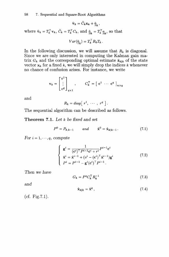
98 7. Sequential and Square-Root Algorithms
Vk = OkXk + !lk '
where Vk = T;[ Vk, Ok = T;[ Ok, and !lk = T;[!lk' so that
Var(!lk) = T"[ RkTk·
In the following discussion, we will assume that Rk is diagonal.Since we are only interested in computing the Kalman gain matrix Gk and the corresponding optimal estimate xklk of the statevector Xk for a fixed k, we will simply drop the indices k wheneverno chance of confusion arises. For instance, we write
andRk = diag [ rI, ... , r q
] .
The sequential algorithm can be described as follows.
Theorem 7.1. Let k be fixed and set
pO = Pk,k-l
For i = 1, ... ,q, compute
and "'0 '"x = Xklk-l' (7.1)
Tben we have
and
(cf. Fig.7.1).
(7.2)
(7.3)
(7.4)
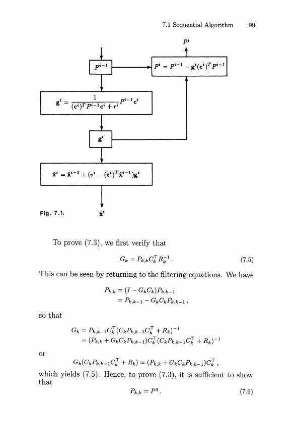
7.1 Sequential Algorithm 99
i 1 pi-l ig = (Ci)T pi-1 Ci + r i C
Fig. 7.1.
To prove (7.3), we first verify that
(7.5)
This can be seen by returning to the filtering equations. We have
Pk,k = (1 - GkCk)Pk,k-l
= Pk,k-l - GkCkPk,k-l ,
so that
Gk = Pk,k-l C"[ (CkPk,k-1C"[ + Rk)-l
= (Pk,k + GkCkPk,k-l)CJ (CkPk,k-lCJ + Rk)-l
orGk(CkPk,k-l C"[ + R k ) = (Pk,k + GkCkPk,k-l)C"[ ,
which yields (7.5). Hence, to prove (7.3), it is sufficient to showthat
(7.6)
100 7. Sequential and Square-Root Algorithms
A direct proof of this identity does not seem to be available.Hence, we appeal to the matrix inversion lemma (Lemma 1.2).Let E> 0 be given, and set P f O = Pk,k-l + El, which is now positivedefinite. Also, set
and
Then by an inductive argument starting with i = 1 and using (1.3)of the matrix inversion lemma, it can be seen that the matrix
is invertible and
Hence, using all these equations for i = q, q - 1, ... ,1, consecutively, we have
q
= (pfO)-l + Lci(ri)-l(ci)Ti=l
On the other hand, again by the matrix inversion lemma, thematrix
is also invertible with
7.1 Sequential Algorithm 101
From the Kalman filtering equations, we have
PE -t pO - pOCk(CkPOC~ + Rk)-l pO
= (1 - GkCk)Pk,k-1 = Pk,k
as € -t 0 ; while from the definition, we have
as € -t o. This means that (7.6) holds so that (7.3) is verified.To establish (7.4), we first observe that
(7.7)
Indeed, since
pi-1 = pi + gi(ei)T pi-1
which follows from the third equation in (7.2), we have, using thefirst equation in (7.2),
. 1 (... T . 1) .g' = ( ·)T p. 1· . p' + g'(c') pt- c'.et t- et + r t
This, upon simplification, is (7.7). Now, from the third equationin (7.2) again, we obtain
for any i, 0 ~ i ~ q - 1. Hence, by consecutive applications of thecorrection equation of the Kalman filter, (7.3), (7.1), (7.8), and(7.7), we have
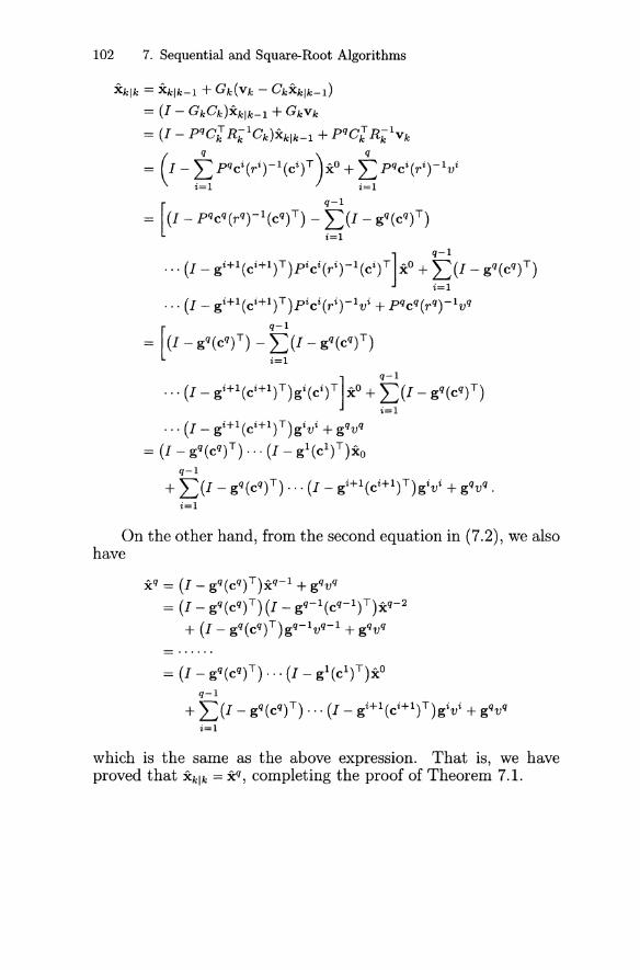
102 7. Sequential and Square-Root Algorithms
Xklk = Xklk-l + Gk(Vk - CkXk1k-l)
= (I - GkCk)Xklk-l + GkVk
= (I - pqC"[ R;;lCk)Xklk_l + pqC"[R;;lVk
= (I - tpqCi(ri)-l(Ci)T)X? + tpqci(ri)-lvi
= [(I - pqcq(rq)-l(cq)T) - ~(I - gq(cq)T)
... (I -gi+l(CHI)T)pici(ri)-I(Ci)T] XO+~ (I - gq(cq)T)
... (I - gi+l(Ci+1)T)pici(ri)-lvi + pqcq(rq)-lvq
= [(I - gq(cq)T) - ~(1 - gq(cq)T)
... {I - gHI(CHI)T)gi(ci)T]XO+ ~(1 - gq(cq)T)
... (I - gi+l(ci+1)T)givi + gqvq
= (I - gq (cq)T) ... (I - g 1( Cl ) T) Xoq-l
+ L(1 - gq(cq)T) ... (I - gi+l(Ci+1)T)givi + gqvq .i=l
On the other hand, from the second equation in (7.2), we alsohave
Xq = (I - gq(cq)T)xq- 1+ gqvq
= (I - gq(cq)T) (I - gq-l(cq- 1)T)xq- 2
+ (I - gq(cq)T)gq-1vq- 1+ gqvq
= (I - gq(cq)T) ... (I - gl(C1)T)xOq-l
+L (I - gq (cq)T) ... (I - gi+l(Ci+1)T)givi + gqvq
i=l
which is the same as the above expression. That is, we haveproved that xklk = x q, completing the proof of Theorem 7.1.
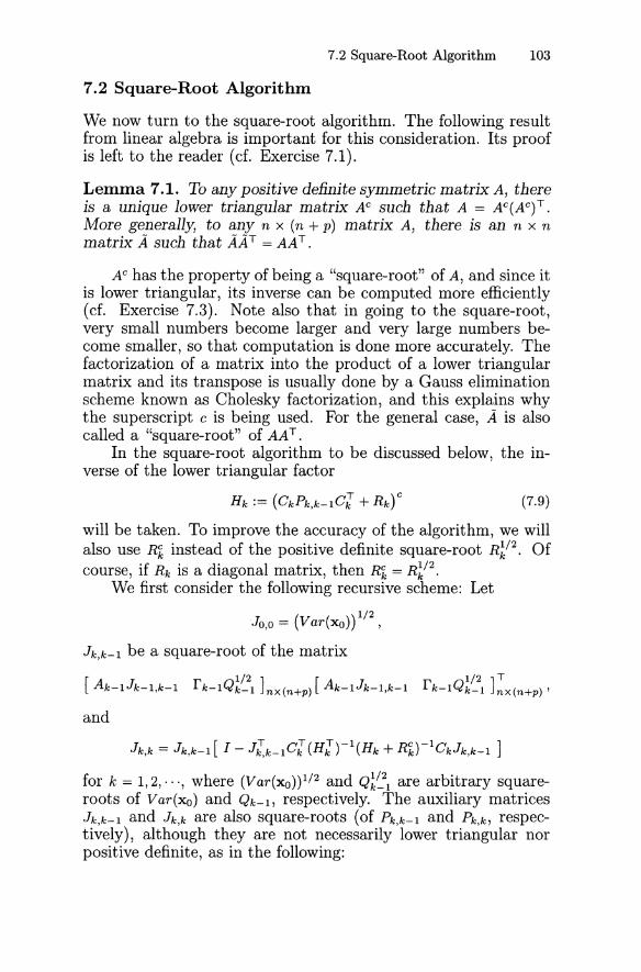
7.2 Square-Root Algorithm 103
7.2 Square-Root Algorithm
We now turn to the square-root algorithm. The following resultfrom linear algebra is important for this consideration. Its proofis left to the reader (cf. Exercise 7.1).
Lemma 7.1. To any positive definite symmetric matrix A, thereis a unique lower triangular matrix AC such that A = AC(AC)T.
More generally, to any n x (n + p) matrix A, there is an n x nmatrix A such that AAT = AAT .
AC has the property of being a "square-root" of A, and since itis lower triangular, its inverse can be computed more efficiently(cf. Exercise 7.3). Note also that in going to the square-root,very small numbers become larger and very large numbers become smaller, so that computation is done more accurately. Thefactorization of a matrix into the product of a lower triangularmatrix and its transpose is usually done by a Gauss eliminationscheme known as Cholesky factorization, and this explains whythe superscript c is being used. For the general case, A is alsocalled a "square-root" of AAT .
In the square-root algorithm to be discussed below, the inverse of the lower triangular factor
Hk:= (CkPk,k-lCl +Rk)C (7.9)
will be taken. To improve the accuracy of the algorithm, we willalso use R k instead of the positive definite square-root R~/2. Ofcourse, if Rk is a diagonal matrix, then R k = R~/2.
We first consider the following recursive scheme: Let
"Jo,o = (Var(xo)) 1/2 ,
Jk,k-l be a square-root of the matrix
[ Ak-lJk-l,k-l
and
r 1/2 ] Tk-lQk-l nx(n+p) '
Jk,k = Jk,k-l [ I - J~k-lC-: (H-:)-l(Hk + Rk)-lCkJk,k-l ]
for k = 1,2,···, where (Var(xo))1/2 and Q~l!l are arbitrary squareroots of Var(xo) and Qk-l, respectively. The auxiliary matricesJk,k-l and Jk,k are also square-roots (of Pk,k-l and Pk,k, respectively), although they are not necessarily lower triangular norpositive definite, as in the following:
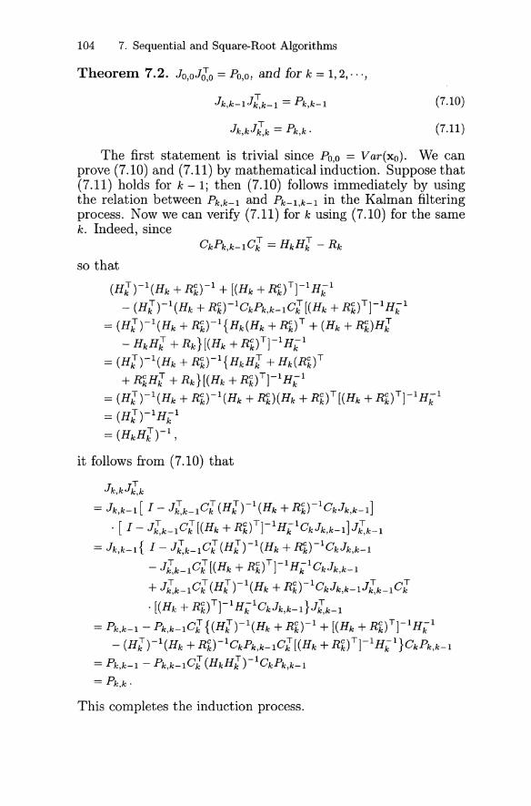
104 7. Sequential and Square-Root Algorithms
Theorem 7.2. Jo,oJ;[,o = Po,o, and for k = 1,2,···,
Jk,k-lJ~k-1= Pk,k-l
Jk,kJ~k = Pk,k .
(7.10)
(7.11)
The first statement is trivial since PO,o = Var(xo). We canprove (7.10) and (7.11) by mathematical induction. Suppose that(7.11) holds for k - 1; then (7.10) follows immediately by usingthe relation between Pk,k-1 and Pk-1,k-1 in the Kalman filteringprocess. Now we can verify (7.11) for k using (7.10) for the samek. Indeed, since
so that
(H~)-l(Hk+ Rk)-l + [(Hk + R k)T]-l Hk1
- (H~)-l(Hk + Rk)-lCkPk,k-1C~[(Hk + Rk)T]-lH;l
= (H~)-l(Hk + Rk)-l{ Hk(Hk + Rk)T + (Hk + Rk)H~
- HkH~ + Rk} [(Hk + R k)T] -1 H;;l
= (H~)-l(Hk + Rk)-l{HkH~ + Hk(Rk)T
+ RkH~ + Rk}[(Hk + R k)T]-lH;;l
= (H~)-l(Hk + Rk)-l(Hk + Rk)(Hk + Rk)T[(Hk + Rk)T]-l H;;l
= (H~)-lH;l
= (HkH~)-l,
it follows from (7.10) that
Jk,kJ~k
= Jk,k-l [ I - J~k-1C~ (H~)-l(Hk + Rk)-lCkJk,k-1]
. [I - J~k_lC~[(Hk +Rk)T]-lH;lCkJk,k_l]J~k_l
= Jk,k-l { I - J~k-lC~ (H~)-l(Hk + Rk)-lCkJk,k-1
- J~k_lC~[(Hk + Rk)T]-lH;lCkJk,k_l
+ J~k-lC~ (H~)-l(Hk + Rk)-lCkJk,k-lJ~k_lC-:
. [(Hk + Rk)T]-lHklCkJk,k-l}J~k_l
= Pk,k-l - Pk,k-lCl {(H;[)-l(Hk + Rk)-l + [(Hk + Rk)T]-l H;;l
- (H~)-l(Hk + Rk)-lCkPk,k-lC~[(Hk + Rk)T]-lH;l }CkPk,k-l
= Pk,k-l - Pk,k-lC~ (HkHJ)-lCkPk,k-l
= Pk,k.
This completes the induction process.
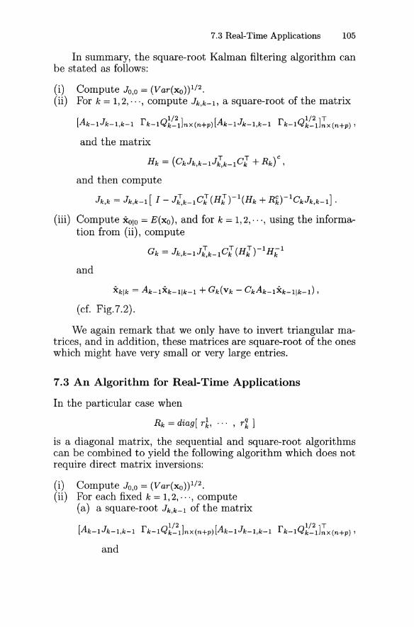
7.3 Real-Time Applications 105
In summary, the square-root Kalman filtering algorithm canbe stated as follows:
(i) Compute Jo,o = (Var(xo))1/2.(ii) For k = 1,2"", c'ompute Jk,k-l, a square-root of the matrix
[Ak-1Jk-l,k-l rk-lQ~~21]nX(n+p)[Ak-lJk-l,k-lrk-lQ~~l]JX(n+p),
and the matrix
Hk = (CkJk,k-lJ~k_lC~ + Rk)C,
and then compute
Jk,k = Jk,k-l [ I - J~k-lC~ (H-:)-l(Hk + Rk)-lCkJk,k-l] .
(iii) Compute xOlo = E(xo), and for k = 1,2" ", using the information from (ii), compute
Gk = Jk,k-lJ~k_1C~ (H-:)-l H"k 1
and
(cf. Fig.7.2).
We again remark that we only have to invert triangular matrices, and in addition, these matrices are square-root of the oneswhich might have very small or very large entries.
7.3 An Algorithm for Real-Time Applications
In the particular case when
Rk = diag[ r~, ... , r% ]
is a diagonal matrix, the sequential and square-root algorithmscan be combined to yield the following algorithm which does notrequire direct matrix inversions:
(i) Compute Jo,o = (Var(xo))1/2.(ii) For each fixed k = 1,2"", compute
(a) a square-root Jk,k-l of the matrix
[A Q1/2 ] [A Q1/2 ]Tk-1 Jk-l,k-1 rk-1 k-1 nx(n+p) k-1 Jk-1,k-1 rk-1 k-1 nx(n+p) ,
and
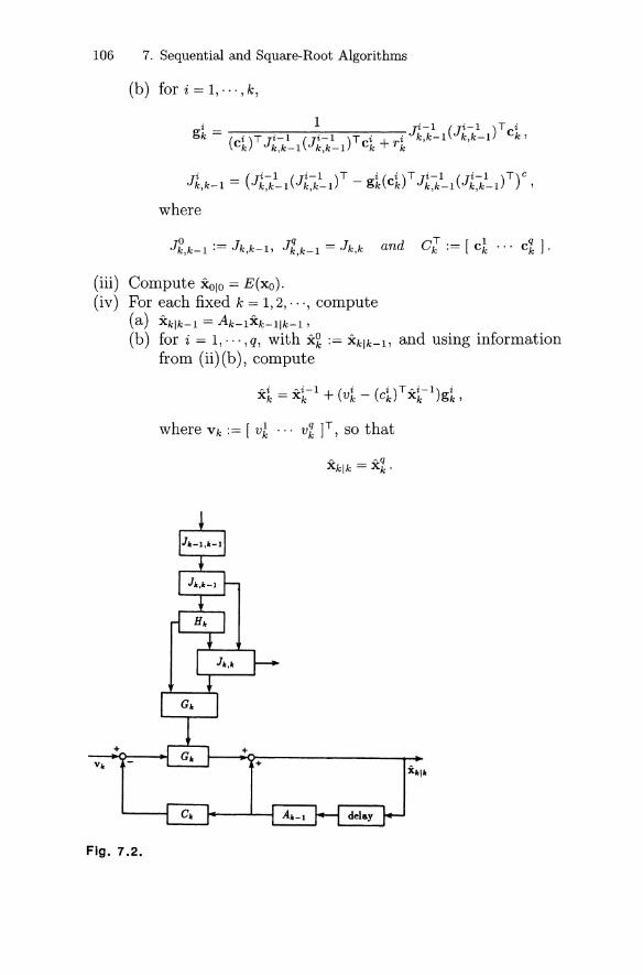
106 7. Sequential and Square-Root Algorithms
(b) for i = 1, .. 0 , k,
Ji (Ji- 1 (Ji-l)T i ( i)T J i- 1 (Ji-1 )T) Ck,k-l = k,k-l k,k-l - gk Ck k,k-l k,k-l ,
where
J o 0- J Jq Jk,k-l'- k,k-l, k,k-l = k,k and cJ:= [cl 000 Ck ]0
(iii) Compute XO/O = E(xo).(iv) For each fixed k = 1,2, 0", compute
(a) xklk-l = Ak-1Xk-llk-l,
(b) for i = 1", ',q, with x~ := xklk-l, and using informationfrom (ii)(b), compute
where Vk := [v~ ... vk ]T, so that
+
Fig. 7.2.
Exercises 107
Exercises
7.1. Give a proof of Lemma 7.1.7.2. Find the lower triangular matrix L that satisfies:
(a) LLT = [; ~ ~].3 2 14
(b) LLT = [~ ~ ;].124
7.3. (a) Derive a formula to find the inverse of the matrix
L = [~~~ £~2 ~],f 31 f 32 f 33
where f 11 ,f22 , and f 33 are nonzero.(b) Formulate the inverse of
f 11 0 0 0f21 f22 0 0
L=
of n1 f n2 fnn
where f 11 , ... ,fnn are nonzero.7.4. Consider the following computer simulation of the Kalman
filtering process. Let € « 1 be a small positive number suchthat
1-€~1
1-€2~1
where "~" denotes equality after rounding in the computer.Suppose that we have
[€2 0]Pk k = 1-€2 ., 0 1
Compare the standard Kalman filter with the square-rootfilter for this example. Note that this example illustrates theimproved numerical characteristics of the square-root filter.
7.5. Prove that to any positive definite symmetric matrix A, thereis a unique upper triangular matrix AU such that A = AU(AU)T.
7.6. Using the upper triangular decompositions instead of thelower triangular ones, derive a new square-root Kalman filter.
7.7. Combine the sequential algorithm and the square-root schemewith upper triangular decompositions to derive a new filtering algorithm.
8. Extended Kalman Filterand System Identification
The Kalman filtering process has been designed to estimate thestate vector in a linear model. If the model turns out to benonlinear, a linearization procedure is usually performed in deriving the filtering equations. We will consider a real-time linear Taylor approximation of the system function at the previousstate estimate and that of the observation function at the corresponding predicted position. The Kalman filter so obtainedwill be called the extended Kalman filter. This idea to handlea nonlinear model is quite natural, and the filtering procedureis fairly simple and efficient. Furthermore, it has found manyimportant real-time applications. One such application is adaptive system identification which we will also discuss briefly inthis chapter. Finally, by improving the linearization procedureof the extended Kalman filtering algorithm, we will introduce amodified extended Kalman filtering scheme which has a parallelcomputational structure. We then give two numerical examplesto demonstrate the advantage of the modified Kalman filter overthe standard one in both state estimation and system parameteridentification.
8.1 Extended Kalman Filter
A state-space description of a system which is not necessarilylinear will be called a nonlinear model of the system. In thischapter, we will consider a nonlinear model of the form
{Xk+l = fk(Xk) + Hk(Xk)~k
Vk = gk(Xk) + '!lk'(8.1)
where fk and gk are vector-valued functions with ranges in Rnand Rq, respectively, 1 :S q :S n, and Hk a matrix-valued functionwith range in Rn X Rq, such that for each k the first order partialderivatives of fk(Xk) and gk(Xk) with respect to all the components
8.1 Extended Kalman Filter 109
of Xk are continuous. As usual, we simply consider zero-meanGaussian white noise sequences {Sk} and {!lk} with ranges in RPand Rq, respectively, 1 ~ p, q ~ n, and
E(Sk!1I) = 0 , E(Skxri )= 0, E(!lkxri )= 0,
for all k and R. The real-time linearization process is carried outas follows.
In order to be consistent with the linear model, the initialestimate Xo = xOlo and predicted position xIlo are chosen to be
Xo = E(xo) , XIlo = fo(xo) .
We will then formulate Xk = xklk, consecutively, for k = 1,2,," ,using the predicted positions
and the linear state-space description
{Xk+I = AkXk + Uk + fkSk
Wk = CkXk + !1k '
(8.2)
(8.3)
where Ak,Uk,rk,Wk and Ck are to be determined in real-time asfollows. Suppose that Xj has been determined so that Xj+Ilj isalso defined using (8.2), for j = 0,1,,,, ,k. We consider the linearTaylor approximation of fk(Xk) at Xk and that of gk(Xk) at xklk-I;that is,
{fk(Xk) ~ fk(Xk) + Ak(Xk - Xk)
gk(Xk) ~ gk(Xklk-l) + Ck(Xk - xklk-l)'
where
(8.4)
and (8.5)
Here and throughout, for any vector-valued function
110 8. Kalman Filter and System Identification
where
we denote, as usual,
~(Xk) ~(x*)
[~(xk)] =x k
8xk k
8Xkill!m (x*) ~(x*)8x~ k 8xk k
Hence, by setting
{
Uk = fk(Xk) - AkXk
fk = Hk(Xk)
Wk = Vk - gk(Xklk-l) + CkXklk-1 ,
(8.6)
(8.7)
the nonlinear model (8.1) is approximated by the linear model(8.3) using the matrices and vectors defined in (8.5) and (8.7) atthe kth instant (cf. Exercise 8.2). Of course, this linearizationis possible only if Xk has been determined. We already have xo,so that the system equation in (8.3) is valid for k = o. Fromthis, we define Xl = XIII as the optimal unbiased estimate (withoptimal weight) of Xl in the linear model (8.3), using the data[vci wJlT. Now, by applying (8.2), (8.3) is established for k = 1,so that X2 = x212 can be determined analogously, using the data[vci wJ wIlT, etc. From the Kalman filtering results for lineardeterministicjstochastic state-space descriptions in Chapters 2and 3 (cf. (2.18) and Exercise 3.6), we arrive at the "correction"formula
Xk = xklk-l + Gk(Wk - CkXk1k-l)
= xklk-l + Gk((Vk - gk(Xklk-l) + CkXklk-l) - CkXklk-l)
= xklk-l + Gk(Vk - gk(Xklk-I))'
where Gk is the Kalman gain matrix for the linear model (8.3) atthe kth instant.
The resulting filtering process is called the extended Kalmanfilter. The filtering algorithm may be summarized as follows (cf.
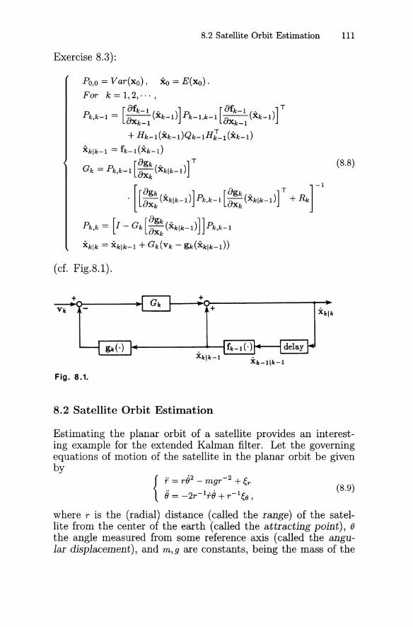
8.2 Satellite Orbit Estimation 111
Exercise 8.3):
Po,o = Var(xo) , Xo = E(xo) .
~or k = 1,2,···,
n [8fk - 1 ("')] [8fk - 1 ('" )] T.Lk,k-l = -8-- Xk-l Pk-1,k-l -8-- Xk-lXk-l Xk-l
+ Hk-l (Xk-l)Qk-lHJ-l (Xk-l)
xklk-l = fk-l(Xk-l)
[8g k '" ] T
Gk = Pk,k-1 8Xk (xklk-d
. [[~:: (Xklk-d] Pk,k-1 [~:: (Xklk-d] T + Rk] -1
Pk,k = [1 - Gk [~;: (Xk lk-1)]] Pk,k-1
Xklk = Xklk-l + Gk(Vk - gk(Xklk-l))
(cf. Fig.8.l).
(8.8)
++
Fig. 8.1.
8.2 Satellite Orbit Estimation
Estimating the planar orbit of a satellite provides an interesting example for the extended Kalman filter. Let the governingequations of motion of the satellite in the planar orbit be givenby
(8.9)
where r is the (radial) distance (called the range) of the satellite from the center of the earth (called the attracting point), ()the angle measured from some reference axis (called the angular displacement), and m,9 are constants, being the mass of the
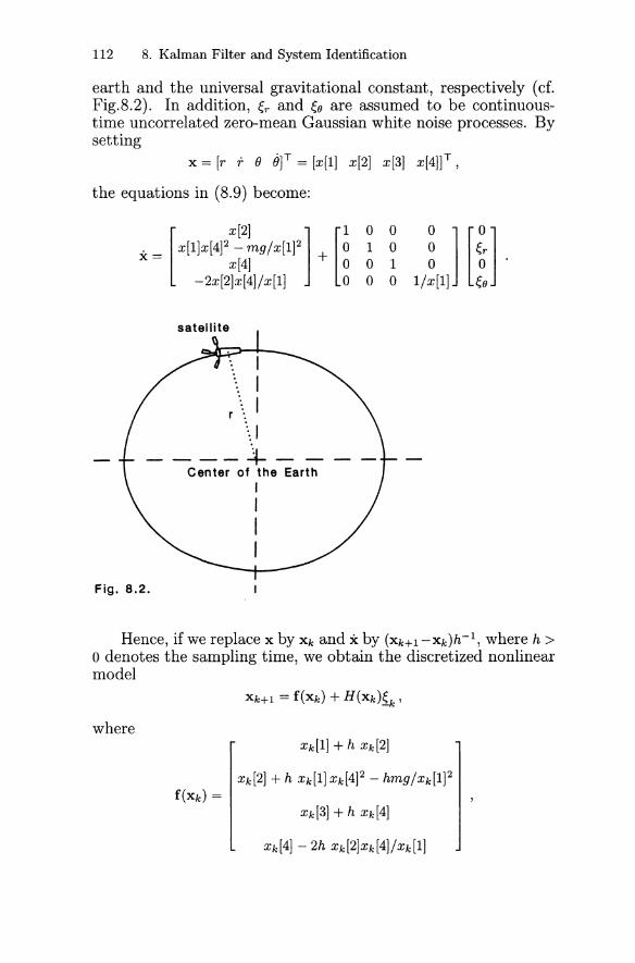
112 8. Kalman Filter and System Identification
earth and the universal gravitational constant, respectively (cf.Fig.8.2). In addition, ~r and ~B are assumed to be continuoustime uncorrelated zero-mean Gaussian white noise processes. Bysetting
x = [r r (J O]T = [x[l] x[2] x[3] x[4]]T,
the equations in (8.9) become:
II
r ... I\1
---+- -Canter of the Earth
IIII
Fig. 8.2.
Hence, if we replace x by Xk and x by (Xk+l -xk)h- 1 , where h >o denotes the sampling time, we obtain the discretized nonlinearmodel
wherexk[l] + h xk[2]
xk[2] + h xk[l] xk[4]2 - hmgjxk[1]2
xk[3] + h xk[4]
xk[4] - 2h Xk[2]Xk[4]/Xk[1]
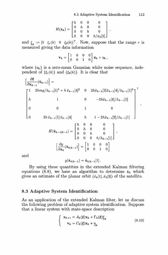
(8.10)
8.3 Adaptive System Identification 113
[
h 0 0 0]o h 0 0H (Xk) = 0 0 hO'
o 0 0 h/xk[l]
and {k := [0 ~r(k) 0 ~e(k)]T. Now, suppose that the range r ismeasured giving the data information
[1 0 0 0]
Vk = 0 0 1 0 Xk + 'f/k ,
where {'f/k} is a zero-mean Gaussian white noise sequence, independent of {~r(k)} and {~e(k)}. It is clear that
[88f (xk-d] =Xk-1
1 2hmg/xk_1[1]3 + hXk_1[4]2 0 2hxk-1 [2] Xk-1 [4] / Xk-1 [1] 2 T
h 1 0 -2hxk-1 [4]/Xk-1 [1]
0 0 1 0
0 2h Xk-1 [1] Xk-1 [4] h 1 - 2hxk-1[2]/Xk-1[1]
H(Xk-1Ik-1) = [~ ~ ~ ~]o 0 0 h/xk-1[1]
[ 8g A ] [1 0 0 00]8Xk (xklk-d = 0 0 1
and9(Xklk-1) = xklk-1[1].
By using these quantities in the extended Kalman filteringequations (8.8), we have an algorithm to determine Xk whichgives an estimate of the planar orbit (xk[1],.xk[3]) of the satellite.
8.3 Adaptive System Identification
As an application of the extended Kalman filter, let us discussthe following problem of adaptive system identification. Supposethat a linear system with state-space description
{Xk+1 = Ak(ft)Xk + fk(ft){k
Vk = Ck(ft)Xk + ~k
114 8. Kalman Filter and System Identification
is being considered, where, as usual, XkERn , ~kERP, !lkERq, 1 ~
p, q ~ n, and {~k} and {!lk} are uncorrelated Gaussian white noisesequences. In this application, we assume that Ak(tl) , rk(tl) , andCk(ft) are known matrix-valued functions of some unknown constant vector fl. The objective is to "identify" fl.
It seems quite natural to set ftk+l = tlk = fl, since tl is a constantvector. Surprisingly, this assumption does not lead us anywhereas we will see below and from the simple example in the nextsection. In fact, fl must be treated as a random constant vectorsuch as
tlk+l = flk + ~k ' (8.11)
where {~k} is any zero-mean Gaussian white noise sequence uncorrelated with {!lk} and with preassigned positive definite variancesVar(~k) = Sk. In applications, we may choose Sk = S > 0 for allk (see Section 8.4). Now, the system (8.10) together with theassumption (8.11) can be reformulated as the nonlinear model:
{
[~:::] = [Ak~:)Xk ] + [rk(~~)~k ](8.12)
Vk = [Ck(~) 0] [~:] +!Zk'
and the extended Kalman filtering procedure can be applied toestimate the state vector which contains ftk as its components.That is, tlk is estimated optimally in an adaptive way. However,in order to apply the extended Kalman filtering process (8.8),we still need an initial estimate ~o := ~Io' One method is toappeal to the state-space description (8.10). For instance, sinceE(vo) = Co(fl)E(xo) so that vo-Co(fl)E(xo) is of zero-mean, we couldstart from k = 0, take the variances of both sides of the modified"observation equation"
Vo - Co(fl)E(xo) = Co(!l.)xo - Co(fl)E(xo) + '!la '
and use the estimate [vo - Co (tl)E(xo)][vo - Co (ft)E(xo)]T for Var(voCo(!l.)E(xo» (cf. Exercise 2.12) to obtain approximately
vovci - Co(fl)E(xo)v6 - vo(Co(!l.)E(xo» T
+ Co(tl) (E(xo)E(xci) - Var(xo»C~ (fl) - Ro = 0 (8.13)
(cf. Exercise 8.4). Now, solve for fl and set one of the "mostappropriate" solutions as the initial estimate~. If there is nosolution of fl in (8.13), we could use the equation
VI = Cl (tl)Xl + !11
= Cl (fl)(Ao(fl)xo + ro(fl)~o) + !11
8.4 Example of Parameter Identification 115
and apply the same procedure, yielding approximately
VI V "[ - C1(fl)Ao(fl)E(xo)v"[ - VI (C1(fl)Ao(fl)E(xo)) T
- C1 (fl)r 0 (fl)Q0 (C1 (fl)r 0 (fl) )T + C1 (fl) Ao(fl) [E (xo)E (xci )
- Var(xo)]Aci (fl)Ci (fl) - RI = 0 (8.14)
(cf. Exercise 8.5), etc. Once ~ has been chosen, we can apply theextended Kalman filtering process (8.8) and obtain the followingalgorithm:
R - [var(xo)0,0 - 0
~or k = 1,2,···,
[ ~klk-l] = [Ak-l(~k-l)Xk-l]-klk-l -k-l
P, - [Ak-l(~k-d :0 [Ak-l(~k-l)Xk-l]] Pk,k-l - 0 - I k-l,k-l
. [Ak-l~~k-l) :~ [Ak-l(~k-l)Xk-l] ] T (8.15)
+ [rk - 1(~k-l)Qk-lrl-l (~k-l) 0]o Sk-l
[" T
Gk = Pk,k-l Ck(flklk- 1) 0]
. [[Ck(~klk-l) O]Pk,k-l [Ck(~klk-l) O]T + Rk]-1
Pk,k = [I - Gk[Ck(~klk-l) 0] ]Pk,k-l
[ ~k] = [~klk-l] + Gk(Vk - Ck(~klk-l)Xklk-l)-k -klk-l
(cf. Exercise 8.6).We remark that if the unknown constant vector fl is consid
ered to be deterministic; that is, flk+1 = flk = fl so that Sk = 0, thenthe procedure (8.15) only yields ~k = ~k-l for all k, independentof the observation data (cf. Exercise 8.7), and this does not giveus any information on ~k. In other words, by using Sk = 0, theunknown system parameter vector fl. cannot be identified via theextended Kalman filtering technique.
8.4 An Example of Constant Parameter Identification
The following simple example will demonstrate how well the extended Kalman filter performs for the purpose of adaptive system
116 8. Kalman Filter and System Identification
identification, even with an arbitrary choice of the initial estimate~o·
Consider a linear system with the state-space description
where a is the unknown parameter that we must identify. Now,we treat a as a random variable; that is, we consider
where ak is the value of a at the kth instant and E((k) == 0,Var((k) == 0.01, say. Suppose that E(xo) == 1, Var(xo) == 0.01, and {1]k}is a zero-mean Gaussian white noise sequence with Var(1]k) == 0.01.The objective is to estimate the unknown parameters ak whileperforming the Kalman filtering procedure. By replacing a withak in the system equation, the above equations become the following nonlinear state-space description:
(8.16)
An application of (8.15) to this model yields
(8.17)
where the initial estimate of Xo is Xo == E(xo) = 1 but ao is unknown.To test this adaptive parameter identification algorithm, we
create two pseudo-random sequences {1]k} and {(k} with zero meanand the above specified values of variances. Let us also (secretely)assign the value of a to be -1 in order to generate the data {Vk}.
To apply the algorithm described in (8.17), we need an initialestimate ao of a. This can be done by using (8.14) with the firstbit of data VI == -1.1 that we generate. In other words, we obtain
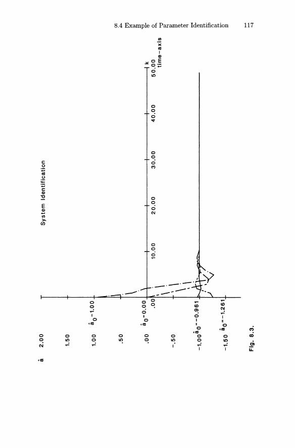
8.4 Example of Parameter Identification 117
en)(
asI
Q)
oE~~;::
oIt)
ooov
00
c: 00 M
-;0-.-....c:Q)
1:)0
E0
Q) 0.... C\ICl)
~
en
00
0,..-
--0--0.--00---" ----- ..----
0 0 0T"'"
T"'"
0 0 ~ co co~
CJ) C\I0 ~
11 11 0 I0 0 I 11cas cas 11 0
0 cas C')cas0 0 0 0 0 0 0 0 CD0 It) 0 ~ ~ ~ 0 Lt)
C\I .".:. ~ I ,..- .,.: ~I I U.
cas
118 8. Kalman Filter and System Identification
0.99a2 + 2.2a + 1.2 = 0
orao = -1.261, -0.961.
In fact, the initial estimate ao can be chosen arbitrarily. In Fig.8.3. we have plots of ak for four different choices of ao, namely:-1.261, -0.961, 0, and 1. Observe that for k ~ 10, all estimates akwith any of these initial conditions are already very close to theactual value a = -1.
Suppose that a is considered to be deterministic, so thatak+l = ak and (8.16) becomes
Then it is not difficult to see that the Kalman gain matrix becomes
for some constant 9k and the "correlation" formula in the filteringalgorithm is
Note that since ak = ak-l = ao is independent of the data {Vk}, thevalue of a cannot be identified.
8.5 Modified Extended Kalman Filter
In this section, we modify the extended Kalman filtering algorithm discussed in the previous sections and introduce a moreefficient parallel computational scheme for system parametersidentification. The modification is achieved by an improved linearization procedure. As a result, the modified Kalman filteringalgorithm can be applied to real-time system parameter identification even for time-varying stochastic systems. We will also givetwo numerical examples with computer simulations to demonstrate the effectiveness of this modified filtering scheme over theoriginal extended Kalman filtering algorithm.
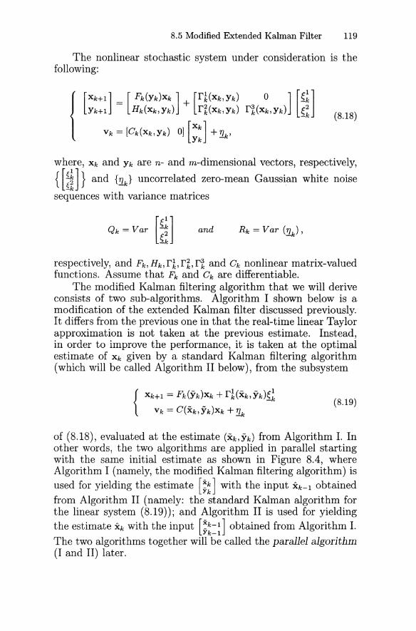
8.5 Modified Extended Kalman Filter 119
The nonlinear stochastic system under consideration is thefollowing:
[Xk+l J [ Fk (Yk)Xk J [rk(Xk, Yk) 0 J [~l]Yk+l = Hk(Xk, Yk) + r~(Xk, Yk) r~(Xk,yk) {~
Vk = [Ck(Xk,Yk) 0] [;:J +!Zk'
(8.18)
where, Xk and Yk are n- and m-dimensional vectors, respectively,
{[iiJ} and {!Zk} uncorrelated zero-mean Gaussian white noise
sequences with variance matrices
and
respectively, and Fk' Hk' rk, r~, r~ and Ck nonlinear matrix-valuedfunctions. Assume that Fk and Ck are differentiable.
The modified Kalman filtering algorithm that we will deriveconsists of two sub-algorithms. Algorithm I shown below is amodification of the extended Kalman filter discussed previously.It differs from the previous one in that the real-time linear Taylorapproximation is not taken at the previous estimate. Instead,in order to improve the performance, it is taken at the optimalestimate of Xk given by a standard Kalman filtering algorithm(which will be called Algorithm 11 below), from the subsystem
{Xk+l = Fk(Yk)Xk + rk(Xk'Yk)~~
Vk = C(Xk, Yk)Xk + !lk(8.19)
of (8.18), evaluated at the estimate (Xk,Yk) from Algorithm I. Inother words, the two algorithms are applied in parallel startingwith the same initial estimate as shown in Figure 8.4, whereAlgorithm I (namely, the modified Kalman filtering algorithm) isused for yielding the estimate [;~] with the input Xk-l obtainedfrom Algorithm 11 (namely: the standard Kalman algorithm forthe linear system (8.19)); and Algorithm 11 is used for yieldingthe estimate Xk with the input [~k-l] obtained from Algorithm I.
Yk-lThe two algorithms together will be called the parallel algorithm(I and 11) later.
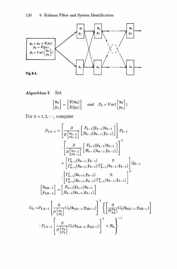
120 8. Kalman Filter and System Identification
Xo = i o = E(xo)Yo = E(yo)
Po = \t"ar ( [;: ] )
Fig. 8.4.
Algorithm I: Set
\
Y/ \
For k == 1,2, . ", compute
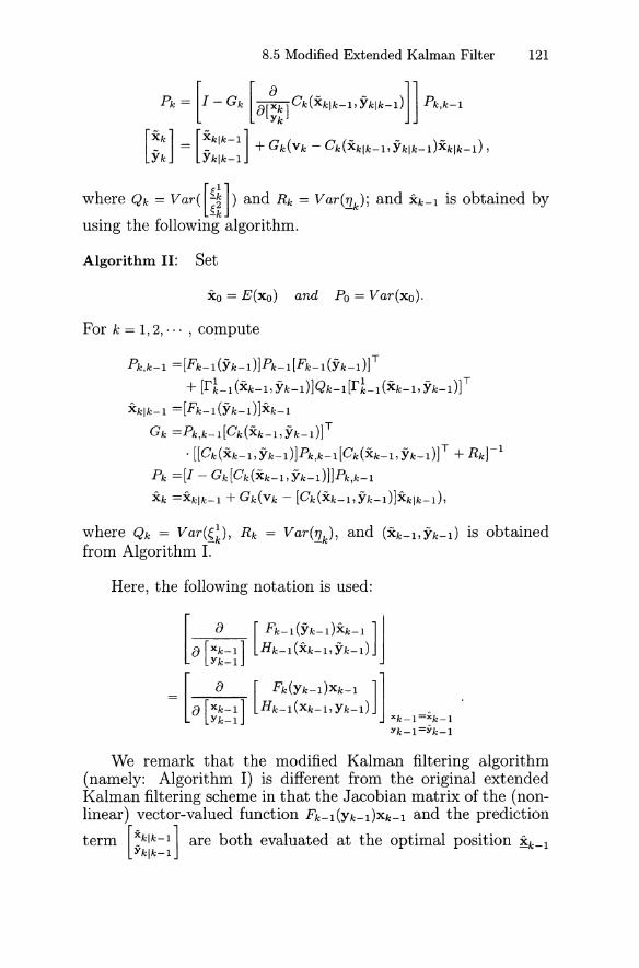
8.5 Modified Extended Kalman Filter 121
where Qk = var([~]) and Rk = Var(!l.k); and Xk-l is obtained by
using the following algorithm.
Algorithm 11: Set
Xo = E(xo) and Po = Var(xo).
For k = 1,2, ... , compute
Pk,k-l =[Fk-l (Yk-l)]Pk-l [Fk-l (Yk_l)]T
+ [fk-l (Xk-l, Yk-l)]Qk-l [fk-l (Xk-l, Yk_l)]T
xklk-l =[Fk-l(Yk-l)]Xk-l
Gk =Pk,k-l[Ck(Xk-l,Yk-l)]T
. [[Ck(Xk-l,Yk-l)]Pk,k-l[Ck(Xk-l,Yk-l)]T + Rk]-l
Pk =[1 - Gk[Ck(Xk-l,Yk-l)]]Pk,k-l
Xk =xklk-l + Gk(Vk - [Ck(Xk-l,Yk-l)]Xklk-l),
where Qk = Var(~~), Rk = Var(!Zk) , and (Xk-l, Yk-l) is obtainedfrom Algorithm I.
Here, the following notation is used:
We remark that the modified Kalman filtering algorithm(namely: Algorithm l) is different from the original extendedKalman filtering scheme in that the Jacobian matrix of the (nonlinear) vector-valued function Fk-l (Yk-l )Xk-l and the prediction
term [~klk-l] are both evaluated at the optimal position ~k-lYklk-l
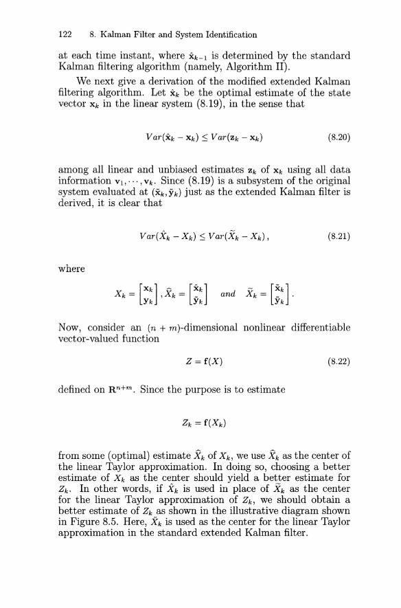
122 8. Kalman Filter and System Identification
at each time instant, where Xk-I is determined by the standardKalman filtering algorithm (namely, Algorithm 11).
We next give a derivation of the modified extended Kalmanfiltering algorithm. Let Xk be the optimal estimate of the statevector Xk in the linear system (8.19), in the sense that
(8.20)
among all linear and unbiased estimates Zk of Xk using all datainformation VI,"', Vk. Since (8.19) is a subsystem of the originalsystem evaluated at (Xk' Yk) just as the extended Kalman filter isderived, it is clear that
(8.21)
where
Now, consider an (n + m)-dimensional nonlinear differentiablevector-valued function
Z = f(X)
defined on Rn+m. Since the purpose is to estimate
(8.22)
from some (optimal) estimate Xk of X k, we use Xk as the center ofthe linear Taylor approximation. In doing so, choosing a betterestimate of Xk as the center should yield a better estimate forZk. In other words, if Xk is used in place of Xk as the centerfor the linear Taylor approximation of Zk, we should obtain abetter estimate of Zk as shown in the illustrative diagram shownin Figure 8.5. Here, Xk is used as the center for the linear Taylorapproximation in the standard extended Kalman filter.
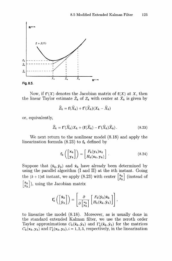
8.5 Modified Extended Kalman Filter 123
z~ -----------
Fig. 8.5.
Now, if f'(X) denotes the Jacobian matrix of f(X) at X, thenthe linear Taylor estimate Zk of Zk with center at Xk is given by
or, equivalently,
(8.23)
We next return to the nonlinear model (8.18) and apply thelinearization formula (8.23) to fk defined by
(8.24)
Suppose that (Xk,Yk) and Xk have already been determined byusing the parallel algorithm (I and 11) at the kth instant. Goingthe (k + l)st instant, we apply (8.23) with center [;~] (instead of
[;~]), using the Jacobian matrix
to linearize the model (8.18). Moreover, as is usually done inthe standard extended Kalman filter, we use the zeroth orderTaylor approximations Ck(Xk, Yk) and rt(Xk, Yk) for the matricesCk(Xk, Yk) and rt(Xk, Yk), i = 1,2,3, respectively, in the linearization
124 8. Kalman Filter and System Identification
of the model (8.18). This leads to the following linear state-spacedescription:
[;::~] = [a [;z] [::g::::)]] [;:] +Uk
[rl(Xk, Yk) 0 ] [~~]
+ r~(xk,h)rHxk,h) ~~
Vk =[Ck(Xk,h) 0) [;:] +!lk'
in which the constant vector
(8.25)
[Fk(Yk)Xk] [ 8 [ Fk(Yk)Xk ]] [Xk]
Uk = Hk(Xk, h) - a [;z] Hk(Xk, h) h
can be considered as a deterministic control input. Hence, similarto the derivation of the standard Kalman filter, we obtain Algorithm I for the linear system (8.25). Here, it should be noted
that the prediction term [~klk-l] in Algorithm I is the only termYklk-l
that contains Uk as formulated below:
[;:::=~] = [a[;~=~] [::~:(~:~2::=:)]] [;:=~] +Uk-l
_ [ 8 [ Fk-l(Yk-l)Xk-l ]] [Xk-l] [Fk-l(Yk-l)Xk-l]- a [;z=~] Hk-l(Xk-llh-l) Yk-l + Hk-l(Xk-llYk-l)
[8 [ Fk-l (Yk-l)Xk-l ]] [~k-l]
- a [;z=~] Hk-l(Xk-llh-d Yk-l
_ [ Fk-l (Yk-l)Xk-l ]- Hk-l(Xk-l,Yk-l) .
8.6 Time-Varying Parameter Identification
In this section, we give two numerical examples to demonstratethe advantage of the modified extended Kalman filter over thestandard one, for both state estimation and system parameteridentification.
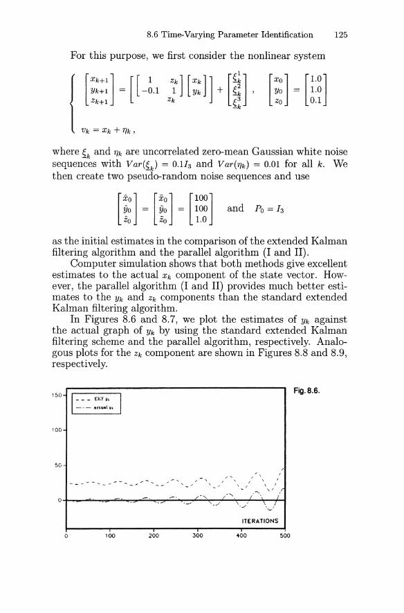
8.6 Time-Varying Parameter Identification 125
For this purpose, we first consider the nonlinear system
[ ~::~] = [[ -~.1 ~k] [::]] + [~i], [~n U:~]-k
where ~k and 'T}k are uncorrelated zero-mean Gaussian white noisesequences with Var(~k) = 0.113 and Var('T}k) = 0.01 for all k. Wethen create two pseudo-random noise sequences and use
[iO] [Xo] [100]~o = ~o = 100Zo Zo 1.0
and Po = 13
as the initial estimates in the comparison of the extended Kalmanfiltering algorithm and the parallel algorithm (1 and 11).
Computer simulation shows that both methods give excellentestimates to the actual Xk component of the state vector. However, the parallel algorithm (1 and 11) provides much better estimates to the Yk and Zk components than the standard extendedKalman filtering algorithm.
In Figures 8.6 and 8.7, we plot the estimates of Yk againstthe actual graph of Yk by using the standard extended Kalmanfiltering scheme and the parallel algorithm, respectively. Analogous plots for the Zk component are shown in Figures 8.8 and 8.9,respectively.
150 1_ - - EKF Yk I- - - actual Yk
100
50
ITERATIONS
Fig. 8.5.
o 100 200 300 400 500
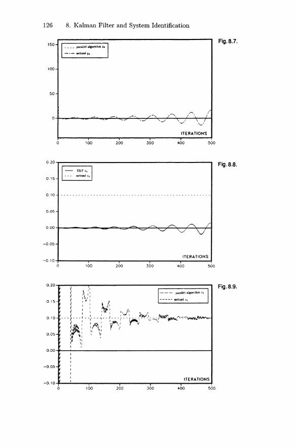
126 8. Kalman Filter and System Identification
150
1_---para1J~1 algorithm '·1--- adualy.
Fig.B.7.
100
50
0/-, /~, I/"~ If
...- "-/'" I
\ /-..../ ~I
ITERATIONS
0 100 200 300 400 500
0.20-.---------------------------......
0.15
Fig. 8.8.
0.10 - - - - _. - - - - - - - - - - - - - - - - - - - - - - - - - - - - - - - - - - - - - - - - - - - --
0.05
-0.05
ITERATIONS-0.10+-----....----....-----...----.....------....
o 100 200 300 400 500
0,15
0.10
0.05
/
--- pllralleoliUgortthm z. I- - - - - actual z.
Fig.8.9.
o.OO-tL-------------------------------t
-0.05
ITERATIONS
500400300200100-0.10 -...:.---.-----....----.....-----....----...
o
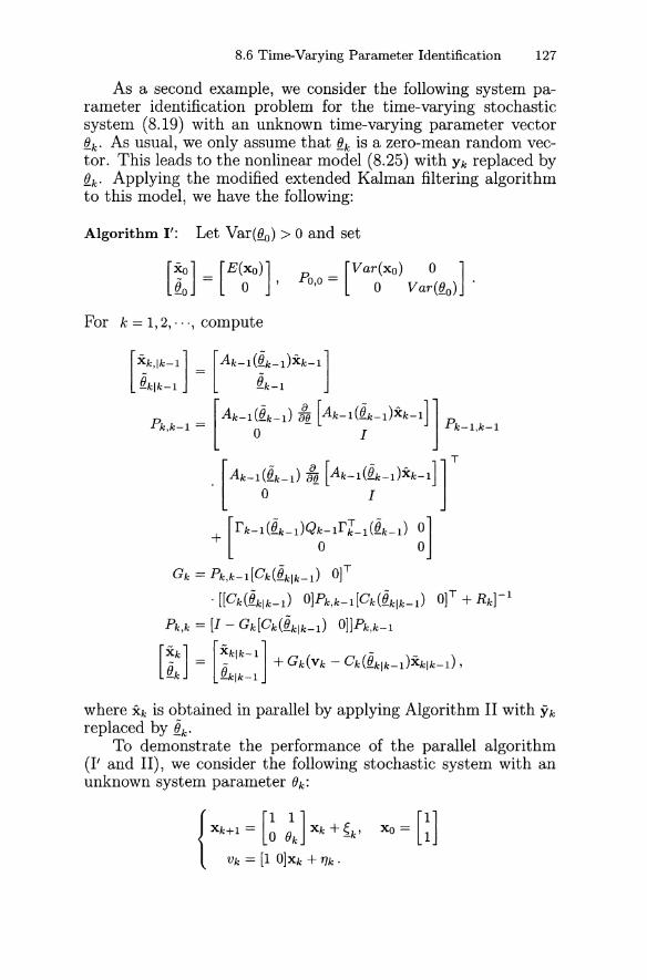
8.6 Time-Varying Parameter Identification 127
As a second example, we consider the following system parameter identification problem for the time-varying stochasticsystem (8.19) with an unknown time-varying parameter vectorflk . As usual, we only assume that flk is a zero-mean random vector. This leads to the nonlinear model (8.25) with Yk replaced byflk. Applying the modified extended Kalman filtering algorithmto this model, we have the following:
Algorithm I': Let Var(flo) > 0 and set
[ XfL~oo] = [E(OXo)] , R = [var(xo) 0 ]0,0 0 Var(flo)·
For k = 1,2, ... , compute
[ ~k'lk-l] = [Ak-l(:k-l)Xk-l]-klk-l -k-l
P = [Ak-l(~k-l) tfJ. [Ak-l(~k_l)Xk-l]] Pk,k-l 0 I k-l,k-l
. [Ak-l~~k-l) tfJ. [Ak-l(~k-l)Xk-l]] T
+ [rk-l(~k-l)Q~-lrLl(~k-l) ~]
- TGk = Pk,k-l[Ck(flkl k- 1 ) 0]
- - T 1. [[Ck(~klk-l) O]Pk,k-l[Ck(fLklk-l) 0] + Rk]-
Pk,k = [I - Gk[Ck(~klk-l) O]]Pk,k-l
[Xk] [Xk1k-l] ........B = B + Gk(Vk - Ck(fLklk-l)Xklk-l) ,-k -klk-l
where Xk is obtained in parallel by applying Algorithm 11 with Ykreplaced by ~k.
To demonstrate the performance of the parallel algorithm(I' and 11), we consider the following stochastic system with anunknown system parameter f)k:
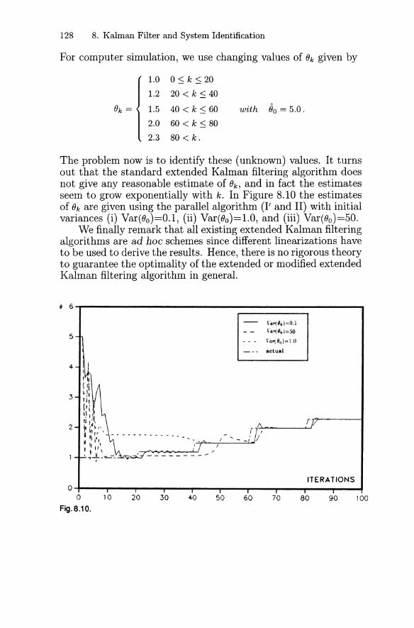
128 8. Kalman Filter and System Identification
For computer simulation, we use changing values of (}k given by
1.0 o :S k :S 20
1.2 20 < k :S 40
(}k == 1.5 40 < k :S 60 with 80 == 5.0.
2.0 60 < k :S 80
2.3 80 < k.
The problem now is to identify these (unknown) values. It turnsout that the standard extended Kalman filtering algorithm doesnot give any reasonable estimate of (}k, and in fact the estimatesseem to grow exponentially with k. In Figure 8.10 the estimatesof (}k are given using the parallel algorithm (I' and 11) with initialvariances (i) Var((}o) ==0. 1, (ii) Var((}0)==1.0, and (iii) Var((}o) ==50.
We finally remark that all existing extended Kalman filteringalgorithms are ad hoc schemes since different linearizations haveto be used to derive the results. Hence, there is no rigorous theoryto guarantee the optimality of the extended or modified extendedKalman filtering algorithm in general.
fJ 6 .....-------------------------.
5
\-ar(fJo)=O.l
\-ar(fJo)=50
\-ar(fJo)=l.O
actual
ITERATIONS
1009080706050403020O-t--....,--..,...---...--......--..--..--.....-...-.II~- ......- .......
o 10
Fig.8.10.
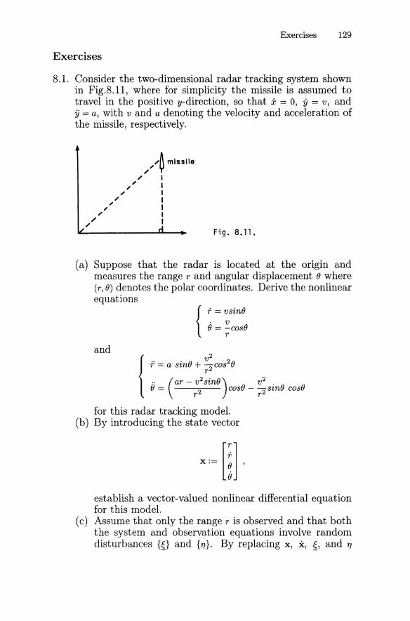
Exercises 129
Exercises
8.1. Consider the two-dimensional radar tracking system shownin Fig.8.ll, where for simplicity the missile is assumed totravel in the positive y-direction, so that x = 0, iJ = v, andjj = a, with v and a denoting the velocity and acceleration ofthe missile, respectively.
Fig. 8. 11 .
(a) Suppose that the radar is located at the orIgIn andmeasures the range r and angular displacement f) where(r, e) denotes the polar coordinates. Derive the nonlinearequations
{r = vsine. ve = -cose
r
and
{
.. . v 2
r = a szne + 2cos2er
.. (ar -v2 sinO) v2
e = r2 cose - r2 sine cose
for this radar tracking model.(b) By introducing the state vector
establish a vector-valued nonlinear differential equationfor this model.
(c) Assume that only the range r is observed and that boththe system and observation equations involve randomdisturbances {{} and {'T]}. By replacing x, x, {, and T/
130 8. Kalman Filter and System Identification
by Xk, (Xk+l - xk)h- 1, 5.k' and 1}k, respectively, where h >
o denotes the sampling time, establish a discrete-timenonlinear system for the above model.
(d) Assume that {5.k} and {1}k} in the above nonlinear system are zero-mean uncorrelated Gaussian white noisesequences. Describe the extended Kalman filtering algorithm for this nonlinear system.
8.2. Verify that the nonlinear model (8.1) can be approximatedby the linear model (8.3) using the matrices and vectorsdefined in (8.5) and (8.7).
8.3. Verify that the extended Kalman filtering algorithm for thenonlinear model (8.1) can be obtained by applying the standard Kalman filtering equations (2.17) or (3.25) to the linearmodel (8.3) as shown in (8.8).
8.4. Verify equation (8.13).8.5. Verify equation (8.14).8.6. Verify the algorithm given in (8.15).8.7. Prove that if the unknown constant vector fl. in the system
(8.10) is deterministic (Le., ftk+1 == flk for all k), then thealgorithm (8.15) fails to identify fl..
8.8. Consider the one-dimensional model
{Xk+l == Xk + ~k
Vk == C x k + 1}k ,
where E(xo) == xo, Var(xo) == Po, {~k} and {1}k} are both zeromean Gaussian white noise sequences satisfying
E(~k~f,) == Qk 8kf, E(1}k1}f) == rk 8kf ,
E(~k1}f) == E(~kXO) == E(1}kXO) == o.
Suppose that the unknown constant c is treated as a randomconstant:
Ck+ 1 == Ck + (k ,
where (k is also a zero-mean Gaussian white noise sequencewith known variances Var((k) == Sk . Derive an algorithm toestimate c. Try the special case where Sk == S > o.
9. Decoupling of Filtering Equations
The limiting (or steady-state) Kalman filter provides a very efficient method for estimating the state vector in a time-invariantlinear system in real-time. However, if the state vector has a veryhigh dimension n, and only a few components are of interest, thisfilter gives an abundance of useless information, an eliminationof which should improve the efficiency of the filtering process. Adecoupling method is introduced in this chapter for this purpose.It allows us to decompose an n-dimensional limiting Kalman filtering algorithm into n independent one-dimensional recursiveformulas so that we may drop the ones that are of little interest.
9.1 Decoupling Formulas
Consider the time-invariant linear stochastic system
{
Xk+l = AXk + rs'kVk = CXk + '!lk'
(9.1)
where all items have been defined in Chapter 6 (cf. Section 6.1for more details). Recall that the limiting Kalman gain matrixis given by
G = PCT (CPCT + R)-l, (9.2)
where p is the positive definite solution of the matrix Riccatiequation
and the steady-state estimate Xk of Xk is given by
Xk = AXk-l + G(Vk - CAXk-l)
= (1 - GC)AXk-l + GVk , (9.4)
132 9. Decoupling of Filtering Equations
(cf. (6.4)). Here, Q and R are variance matrices defined by
and
for all k (cf. Section 6.1). Let <I> = (1 - GC)A := [cPij]nxn, G =
[9ij]nxq, 1::; q ::; n, and set
and
We now consider the z-transforms
<X>
X j = Xj(z) = LXk,jZ-k,k=O
<X>
Vj = Vj(z) = L Vk,jZ-k ,k=O
j = 1,2,··· ,n,
j = 1,2,··· ,n,(9.5)
of the jth components of {Xk} and {Vk}, respectively. Since (9.4)can be formulated as
n q
Xk+l,j = L cPjiXk,i + L 9jiVk+l,ii=l i=l
for k = 0,1,··· , we have
n q
zXj = L cPjiXi + ZL9jiVi·i=l i=l
Hence, by settingA = A(z) = (z1 - <1»,
we arrive at
(9.6)
Note that for large values of Izl, A is diagonal dominant andis therefore invertible. Hence, Cramer's rule can be used to solvefor Xl, ... ,Xn in (9.6). Let Ai be obtained by replacing the ithcolumn of A with
zG [J.] .
9.1 Decoupling Formulas 133
Then, detA and detA i are both polynomials in z of degree n, and
(9.7)
i = 1, ... ,n. In addition, we may write
where
b1 = -(AI + A2 + ... + An) ,
b2 = (AI A2 + AI A3 + ... + AI An + A2 A3 + ... + An -lAn) ,
with Ai, i = 1,2, .. " n, being the eigenvalues of matrix q>. Similarly,we have
detA i = (~c}zn-i) VI + ... + (~cizn-i)Vi, (9.9)
where c~, R = 0,1,' .. ,n, i = 1,2,"" q, can also be computed explicitly. Now, by substituting (9.8) and (9.9) into (9.7) and thentaking the inverse z-transforms on both sides, we obtain the following recursive (decoupling) formulas:
Xk,i = - b1X k-l,i - b2 X k-2,i - - bnXk-n,i
+ C6 Vk,1 + C~Vk-l,l + + C~Vk-n,1
+ C6 Vk,q + CiVk-l,q + ... + C~Vk-n,q, (9.10)
i = 1,2,' .. ,n. Note that the coefficients b1 , ... ,bn and cb, ... ,c~, i =1," . ,q, can be computed before the filtering process is applied.We also remark that in the formula (9.10), each Xk,i depends onlyon the previous state variables Xk-l,i, ... ,Xk-n,i and the data information, but not on any other state variaples Xk-l,j with j =1= i.This means that the filtering formula (9.4) has been decomposedinto n one-dimensional recursive ones.
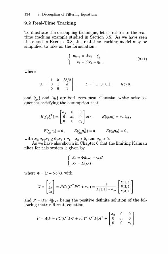
134 9. Decoupling of Filtering Equations
9.2 Real-Time Tracking
To illustrate the decoupling technique, let us return to the realtime tracking example studied in Section 3.5. As we have seenthere and in Exercise 3.8, this real-time tracking model may besimplified to take on the formulation:
where
{Xk+l == AXk + ~k
Vk == CXk + 1Jk ,(9.11)
[
1 h h2 /2]A== 0 1 h ,
o 0 1C==[l 00], h > 0,
and {~k} and {1}k} are both zero-mean Gaussian white noise sequences satisfying the assumption that
with ap , av, aa 2: 0, ap + av + aa > 0, and am > o.As we have also shown in Chapter 6 that the limiting Kalman
filter for this system is given by
where q> == (1 - GC)A with
and P == [P[i, j]]3X3 being the positive definite solution of the following matrix Riccati equation:
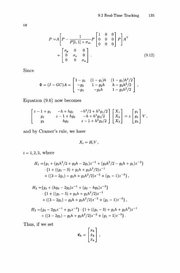
9.2 Real-Time 'fracking 135
or
Since
Equation (9.6) now becomes
[
Z-1+ 91 -h+h91 -h2/2+h291 /2] [Xl] [91]
92 Z - 1 + h92 -h + h292/2 XX32 = Z 99
2
3
V,93 h93 Z - 1 + h293/2
and by Cramer's rule, we have
i = 1,2,3, where
HI ={91 + (93 h2 / 2 + 92 h - 291)Z-1 + (93 h2 / 2 - 92h + 91)Z~2}
. {I + ((91 - 3) + 92h + 93h2 /2)z-1
+ ((3 - 291) - 92h + 93h2 /2)Z-2 + (91 -1)z-3},
H2 ={92 + (h93 - 292)Z-1 + (92 - h93)Z-2}
. {I + ((91 - 3) + 92h + 93h2 /2)Z-1
+ ((3 - 291) - 92h + 93h2 /2)Z-2 + (91 - 1)z-3},
H3 ={93 - 293Z- 1+ 93 Z- 2} . {I + ((91 - 3) + 92h + 93 h2 )z-1
+ ((3 - 291) - 92h + 93h2/2)Z-2 + (91 - 1)z-3}.
Thus, if we set
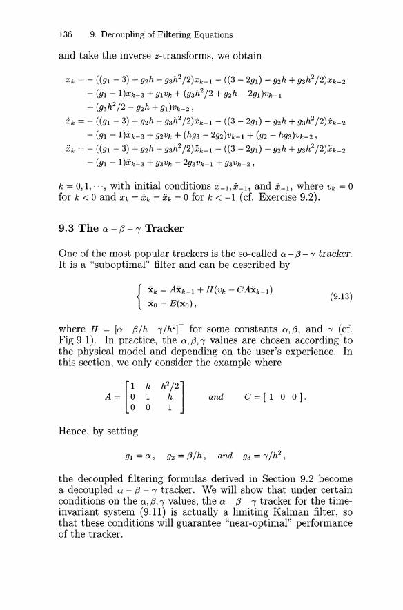
136 9. Decoupling of Filtering Equations
and take the inverse z-transforms, we obtain
Xk = - ((91 - 3) + 92 h + 93 h2 /2)Xk-l - ((3 - 291) - 92h + 93 h2 /2)Xk-2
- (91 - 1)xk-3 + 91Vk + (93 h2 / 2 + 92 h - 291)Vk-l
+ (93 h2 / 2 - 92 h + 91)Vk-2 ,
Xk = - ((91 - 3) + 92 h + 93 h2 /2)Xk-l - ((3 - 291) - 92 h + 93 h2 / 2)Xk-2
- (91 - 1)xk-3 + 92Vk + (h93 - 292)Vk-l + (92 - h93)Vk-2 ,
Xk = - ((91 - 3) + 92 h + 93 h2 /2)Xk-l - ((3 - 291) - 92 h + 93 h2 /2)Xk-2
- (91 - 1)xk-3 + 93Vk - 293Vk-l + 93Vk-2 ,
k = 0,1,···, with initial conditions X-I, X-I, and X-I, where Vk = 0for k < 0 and Xk = Xk = Xk = 0 for k < -1 (cf. Exercise 9.2).
9.3 The a - (3 -, Tracker
One of the most popular trackers is the so-called a - (3 -, tracker.It is a "suboptimal" filter and can be described by
{Xk = AXk-l + H(Vk - CAXk-l)
Xo = E(xo),(9.13)
where H = [a (3/h ,/h2]T for some constants a, (3, and, (cf.Fig.9.1). In practice, the a,(3" values are chosen according tothe physical model and depending on the user's experience. Inthis section, we only consider the example where
Hence, by setting
and C=[l 00].
91=a, 92 = (3/h, and 93=,/h2 ,
the decoupled filtering formulas derived in Section 9.2 becomea decoupled a - (3 -, tracker. We will show that under certainconditions on the a, (3" values, the a - (3 - , tracker for the timeinvariant system (9.11) is actually a limiting Kalman filter, sothat these conditions will guarantee "near-optimal" performanceof the tracker.
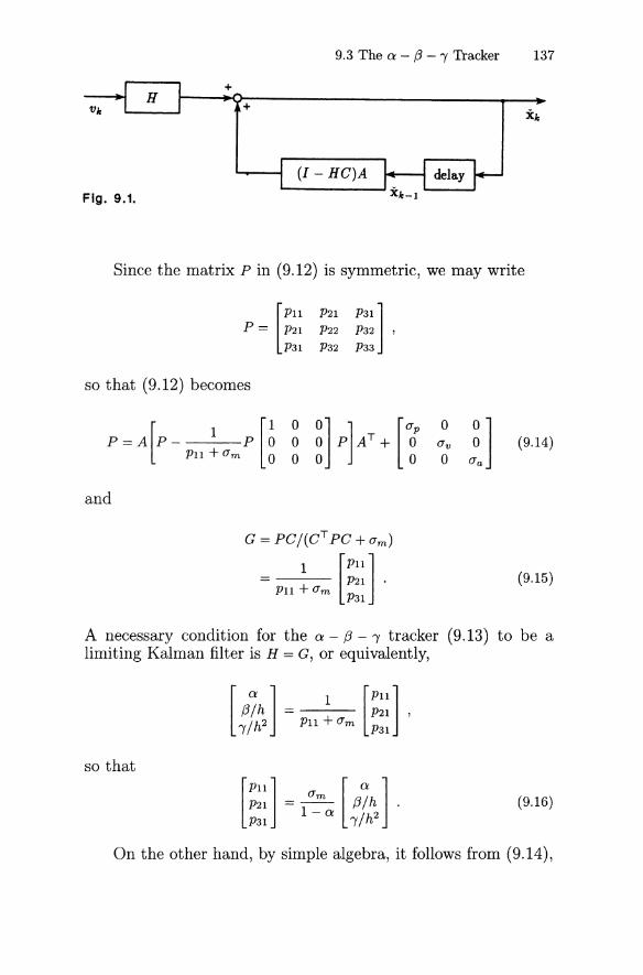
9.3 The a - (3 - , Tracker 137
+
(I - HC)A
Fig. 9.1.
Since the matrix P in (9.12) is symmetric, we may write
[PH P2I P31 ]P = P2I P22 P32 ,
P3I P32 P33
so that (9.12) becomes
[ [1 0
~]P]AT+[I0
~JP=AP- 1 PO 0 avPII + am 0 0 0
and
G = PCj(CT PC + am)
1 [PII]= P2I .PII + am P3I
(9.14)
(9.15)
A necessary condition for the a - (3 - , tracker (9.13) to be alimiting Kalman filter is H = G, or equivalently,
[ a] 1 [PI1](3jh = P2I ,,jh2 PII + am P31
so that
[ ~~~] = l~a [jJ/~] .P3I ,jh
(9.16)
On the other hand, by simple algebra, it follows from (9.14),
138 9. Decoupling of Filtering Equations
(9.15), and (9.16) that
[
PII P2I P3I ]P2I P22 P32 =P3I P32 P33
PII + 2hp2I + h2p3I+h2p22 + h3p32 + h4 p33/4
P2I + hP3I + hP22+3h2p32/2 + h3p33/2
P2I + hP3I + hP22+3h2p32/2 + h3p33/2
P32 + hP33
P3I + hP32+h2p33/2
P32 + hP33
P33
(a + (3)2 (a(3 + a, + (32 ,(a + (3+,(a + (3 + ,/4) +3,8,/2 +,2 /2)/h +,/2)/h2
1(a(3 + a, + (32 ((3 + ,)2/h2 ,((3 + ,)/h3
PII + am +3(3,/2 +,2 /2)/h
,(a+(3+,/2)/h2 ,((3 + ,)/h3 ,2/h4
[ ap 0
~] .+ 0 av
0 0 aa
Substituting (9.16) into the above equation yields
h4
2 aa =PII+ am,h4 ((3+,)2 h
PII = ,3(2a + 2(3 + ,) aa - ,(2a + 2(3 + ,) av
2hp2I + h2p3I + h2p22 (9.17)
h4 h2
= -42(4a2 + 8a(3 + 2(32 + 4a, + ,8,)aa + -av - ap, 2
h4 3P31 + P22 = 4'"12 (40: + (3)((3 + '"1)aa + 4"av ,
andP22 = (1 ~:)h2 [(3(0: + (3 + '"1/4) - '"1(2 + 0:)/2]
am )P32 = (1 _ 0:)h3'"1(0: + (3/2
P33 = (1 ~:)h4 '"1((3 + '"1) .
(9.18)
9.4 An Example 139
Hence, from (9.16), (9.17) , and (9.18) we have
0" 1.J!.... = -l-(o? + a(3 + a'Y/2 - 2(3)O"rn - aO"v 1 2 -2- = --((3 - 2a'Y)hO"rn 1 - a
O"a = _1_'Y2h- 4
O"rn 1 - a
and
(9.19)
[
a (3/h 'Y/h2 ]P =~ f3/h (f3(a + (3 + 'Y/4) - 'Y(2 + a)/2)/h2 'Y(a + f3/2)/h 3
1 - a 'Y/h2 'Y(a + (3/2)/h3 'Y((3 + 'Y)/h4
(9.20)(cf. Exercise 9.4). Since P must be positive definite (cf. Theorem6.1), the a,(3,'Y values can be characterized as follows (cf. Exercise9.5):
Theorem 9.1. Let the a,(3,'Y values satisfy the conditions in(9.19) and suppose that O"rn > o. Then the a - f3 - 'Y tracker is alimiting Kalman filter if and only if the following conditions aresatisfied:(i) 0 < a < 1 , 'Y > 0,(ii) y'2a'Y 5: (3 5: 2~Q (ex + 'Y/2), and(iii) the matrix
p = [~ ,6(a + ,6 + 1'/~ - 1'(2 + 1')/2 1'(a: ,6/2)]'Y 'Y(a + (3/2) 'Y((3 + 'Y)
is non-negative definite.
9.4 An Example
Let us now consider the special case of the real-time trackingsystem (9.11) where O"p = O"v = 0 and O"a,O"rn > o. It can be verifiedthat (9.16-18) together yield
(9.21)
where
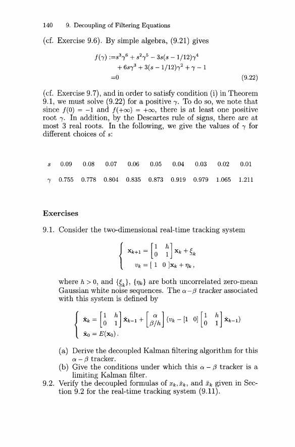
140 9. Decoupling of Filtering Equations
(cf. Exercise 9.6). By simple algebra, (9.21) gives
f(,) :=83,6 + 82,5 -38(8 - 1/12),4
+ 68,3 + 3(8 - 1/12),2 +, - 1
=0 (9.22)
(cf. Exercise 9.7), and in order to satisfy condition (i) in Theorem9.1, we must solve (9.22) for a positive,. To do so, we note thatsince f(O) = -1 and f(+oo) = +00, there is at least one positiveroot,. In addition, by the Descartes rule of signs, there are atmost 3 real roots. In the following, we give the values of , fordifferent choices of 8:
8 0.09 0.08 0.07 0.06 0.05 0.04 0.03 0.02 0.01
, 0.755 0.778 0.804 0.835 0.873 0.919 0.979 1.065 1.211
Exercises
9.1. Consider the two-dimensional real-time tracking system
where h > 0, and {Sk}' {TJk} are both uncorrelated zero-meanGaussian white noise sequences. The a-f3 tracker associatedwith this system is defined by
{
Xk = [~ ~] Xk-l + [/J/h] (Vk - [1 0] [~ ~] Xk-l)
Xo == E(xo).
(a) Derive the decoupled Kalman filtering algorithm for thisa - f3 tracker.
(b) Give the conditions under which this a - f3 tracker is alimiting Kalman filter.
9.2. Verify the decoupled formulas of Xk,Xk, and Xk given in Section 9.2 for the real-time tracking system (9.11).
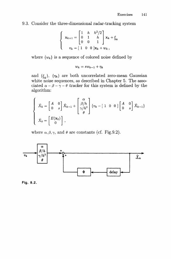
+
Exercises 141
9.3. Consider the three-dimensional radar-tracking system
{[
1 h h2 /2]Xk+l = ~ ~ ~ Xk + ~k
Vk = [1 0 0 ]Xk + Wk ,
where {Wk} is a sequence of colored noise defined by
Wk = SWk-l + TJk
and {{k}' {TJk} are both uncorrelated zero-mean Gaussianwhite noise sequences, as described in Chapter 5. The associated a - {3 - '1 - (J tracker for this system is defined by thealgorithm:
Xk = [~ ~] Xk- 1 + [~~~ ] {Vk - [1 0 0] [~ ~] Xk-d
Xo = [E~o)] ,
where a, {3, '1, and (J are constants (cf. Fig.9.2).
Cl
---.I {J/h t---.....+{>---------------..--..i/h2
(J
Fig. 9.2.
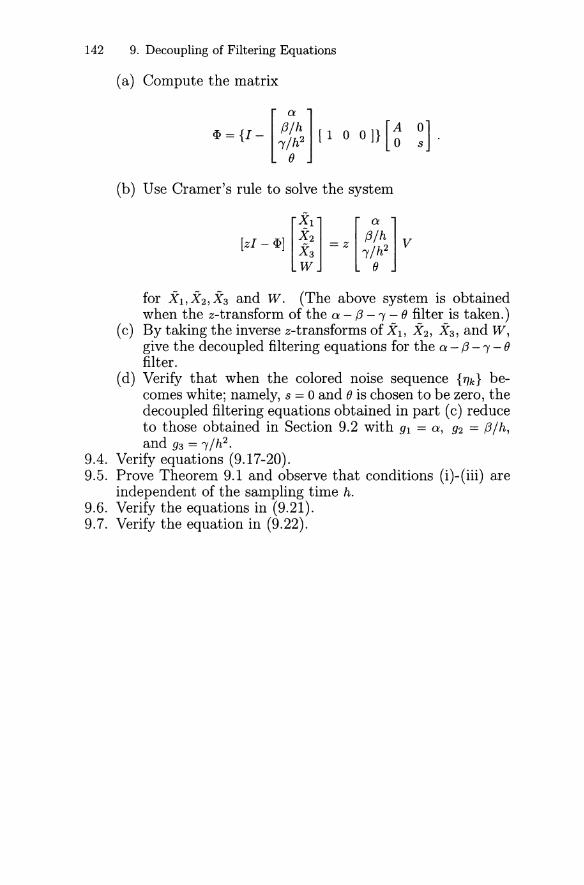
142 9. Decoupling of Filtering Equations
(a) Compute the matrix
~ = {I - [~~~ ] [1 0 O]} [~ ~].
(b) Use Cramer's rule to solve the system
for Xl ,X2 ,X3 and W. (The above system is obtainedwhen the z-transform of the Cl! - f3 -, - () filter is taken.)
(c) By taking the inverse z-transforms of Xl, X2 , X3 , and W,give the decoupled filtering equations for the Cl! - f3 -,- ()filter.
(d) Verify that when the colored noise sequence {17k} becomes white; namely, s = 0 and () is chosen to be zero, thedecoupled filtering equations obtained in part (c) reduceto those obtained in Section 9.2 with 91 = Cl!, 92 = f3/h,and 93 = ,/h2
•
9.4. Verify equations (9.17-20).9.5. Prove Theorem 9.1 and observe that conditions (i)-(iii) are
independent of the sampling time h.9.6. Verify the equations in (9.21).9.7. Verify the equation in (9.22).
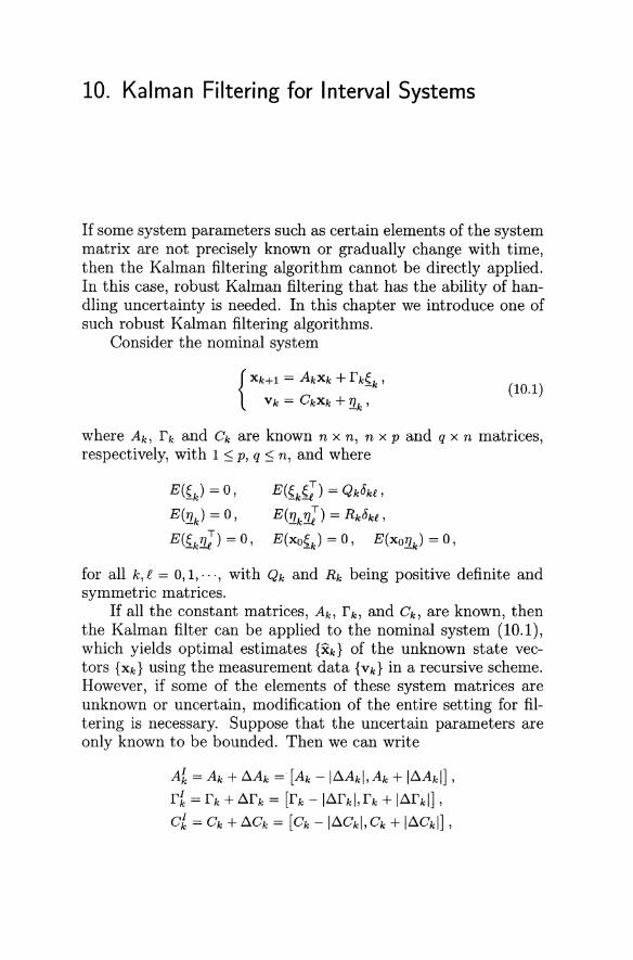
10. Kalman Filtering for Interval Systems
If some system parameters such as certain elements of the systemmatrix are not precisely known or gradually change with time,then the Kalman filtering algorithm cannot be directly applied.In this case, robust Kalman filtering that has the ability of handling uncertainty is needed. In this chapter we introduce one ofsuch robust Kalman filtering algorithms.
Consider the nominal system
{Xk+l = AkXk + rk~k '
Vk = CkXk + '!lk '(10.1)
where Ak, rk and Ck are known n x n, n x p and q x n matrices,respectively, with 1 ~ p, q ::; n, and where
E(~k) = 0,
E('!lk) = 0,
E(~k!1.J) = 0,
E(~k(J) = Qkbki ,
E('!lk!1.J) = Rkbki ,
E(xo~k) = 0 , E(xO'!lk) = 0 ,
for all k, f = 0,1"", with Qk and Rk being positive definite andsymmetric matrices.
If all the constant matrices, Ak, r k , and Ck, are known, thenthe Kalman filter can be applied to the nominal system (10.1),which yields optimal estimates {Xk} of the unknown state vectors {Xk} using the measurement data {Vk} in a recursive scheme.However, if some of the elements of these system matrices areunknown or uncertain, modification of the entire setting for filtering is necessary. Suppose that the uncertain parameters areonly known to be bounded. Then we can write
Ak = Ak + ~Ak =" [Ak -1~Akl, Ak + I~AkIJ '
rk = rk + ~rk = [rk -I~rkl,rk + l~rklJ 'c£ = Ck + ~Ck = [Ck -1~Ckl, Ck + I~CkIJ ,
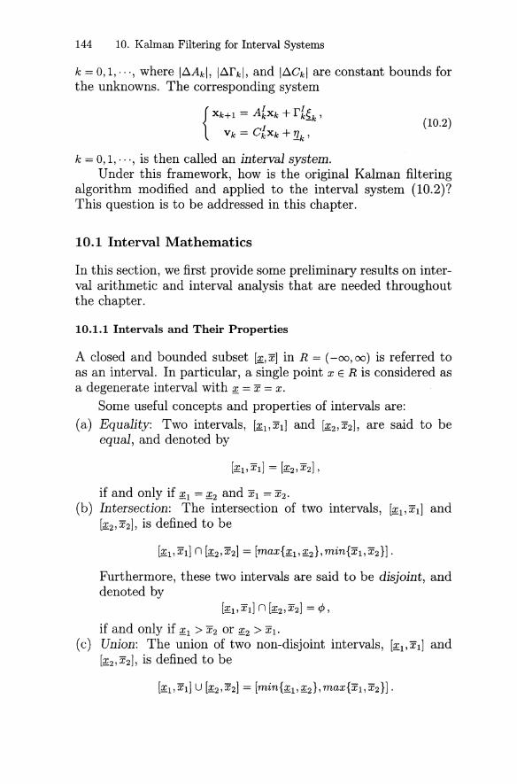
144 10. Kalman Filtering for Interval Systems
k == 0,1"", where I~Akl, I~rkl, and I~Ckl are constant bounds forthe unknowns. The corresponding system
{
Xk+l = A~Xk + r'~k 'Vk == CkXk +!1.k '
(10.2)
k == 0,1" . " is then called an interval system.Under this framework, how is the original Kalman filtering
algorithm modified and applied to the interval system (10.2)?This question is to be addressed in this chapter.
10.1 Interval Mathematics
In this section, we first provide some preliminary results on interval arithmetic and interval analysis that are needed throughoutthe chapter.
10.1.1 Intervals and Their Properties
A closed and bounded subset [~, x] in R == (-00, 00) is referred toas an interval. In particular, a single point x E R is considered asa degenerate interval with ~ == x == x.
Some useful concepts and properties of intervals are:
(a) Equality: Two intervals, [~l' Xl] and [~2' X2], are said to beequal, and denoted by
if and only if ~l == ~2 and Xl == X2.(b) Intersection: The intersection of two intervals, [~l' Xl] and
[~2' X2], is defined to be
[~I,XI] n [~2,X2] == [max{~I'~2},min{xI,x2}]'
Furthermore, these two intervals are said to be disjoint, anddenoted by
[~I,XI] n [~2,X2] == cP,
if and only if ~l > X2 or ~2 > Xl.(c) Union: The union of two non-disjoint intervals, [~I,XI] and
[~2' X2], is defined to be
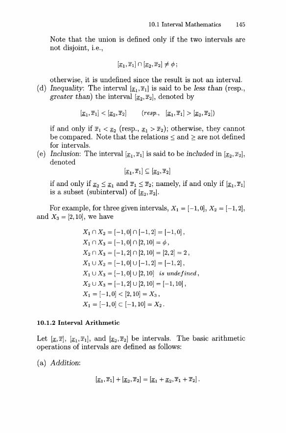
10.1 Interval Mathematics 145
Note that the union is defined only if the two intervals arenot disjoint, i.e.,
otherwise, it is undefined since the result is not an interval.(d) Inequality: The interval [~l' Xl] is said to be less than (resp.,
greater than) the interval [~2' X2], denoted by
if and only if Xl < ~2 (resp., ~l > X2); otherwise, they cannotbe compared. Note that the relations ~ and 2: are not definedfor intervals.
(e) Inclusion: The interval [~l' Xl] is said to be included in [~2' X2],denoted
[~l' Xl] ~ [~2' X2]
if and only if ~2 ~ ~l and Xl ~ X2; namely, if and only if [~l' Xl]is a subset (subinterval) of [~2,X2].
For example, for three given intervals, Xl == [-1,0], X2 == [-1,2],and X3 == [2,10], we have
Xl n X 2 == [-1,0] n [-1,2] == [-1,0],
Xl n X 3 == [-1,0] n [2,10] == cjJ,
X2 n X3 == [-1,2] n [2,10] == [2,2] == 2,
Xl U X 2 == [-1,0] U [-1,2] == [-1,2],
Xl U X3 == [-1,0] U [2,10] is undefined,
X2 U X3 == [-1,2] U [2,10] == [-1,10] ,
Xl == [-1,0] < [2,10] == X 3 ,
Xl == [-1,0] C [-1,10] == X 2 •
10.1.2 Interval Arithmetic
Let [~, x], [;fl' Xl], and [;f2' X2] be intervals. The basic arithmeticoperations of intervals are defined as follows:
(a) Addition:
146 10. Kalman Filtering for Interval Systems
(b) Subtraction:
[;£1' Xl] - [~2' X2] = [~l - X2, Xl - ~2] .( C) Reciprocal operation:
If 0 tt [~,x] then [;f.,X]-l = [l/x, 1/;f.];
If 0 E [~,x] then [~,x]-l is undefined.
(d) Multiplication:
wherey.. = min {;£1~2 , ~lX2 , Xl~2 , XlX2} ,
y = max {;f.l~2' ~lX2, Xl;f.2' XlX2} .
(e) Division:[;£1' Xl] / [~2,X2] = [;£1' Xl] . [~2,X2]-1,
provided that 0 tt [;f.2' X2]; otherwise, it is undefined.
For three intervals, X = [;f., x], Y = [y, y], and Z = [~, z], considerthe interval operations of addition (+)~ subtraction (-), multiplication (.), and division (/), namely,
Z=X*Y, * E {+,-,., I}.
It is clear that X * Y is also an interval. In other words, thefamily of intervals under the four operations {+, -, . , /} is algebraically closed. It is also clear that the real numbers x, y, z,· ..are isomorphic to degenerate intervals [x, x], [y, y], [z, z], ... , so wewill simply denote the point-interval operation [x, x] * Y as x * Y.Moreover, the multiplication symbol "." will often be droppedfor notational convenience.
Similar to conventional arithmetic, the interval arithmetichas the following basic algebraic properties (cf. Exercise 10.1):
X+Y=Y+X,
Z + (X + Y) = (Z + X) + Y ,
XY=YX,
Z(XY) = (ZX)Y,
X + 0 = 0 + X = X and XO = OX = 0, where 0 = [0,0] ,
X1=1X=X, where /=[1,1],
Z(X + Y) ~ ZX + ZY, where = holds only if either
(a) Z = [z,z],
(b)X=Y=O, or
(c) xy ~ 0 for all x E X and y E Y .
10.1 Interval Mathematics 147
In addition, the following is an important property of intervaloperations, called the monotonic inclusion property.
Theorem 10.1. Let Xl, X 2 , YI , and Y2 be intervals, with
and
Then for any operation * E {+, -, . , I}, it follows that
This property is an immediate consequence of the relationsXl ~ YI and X 2 ~ Y2 , namely,
Xl *X2 = {Xl *x2l x I E X I ,X2 E X 2 }
~ {YI * Y21 YI E YI , Y2 E Y2 }
=YI *Y2 .
Corollary 10.1. Let X and Y be intervals and let X E X and Y E Y.Then,
for all * E {+, -, . , /} .
What is seemingly counter-intuitive in the above theorem andcorollary is that some operations such as reciprocal, subtraction,and division do not seem to satisfy such a monotonic inclusionproperty. However, despite the above proof, let us consider asimple example of two intervals, X = [0.2,0.4] and Y = [0.1,0.5].Clearly, X ~ Y. We first show that fiX ~ flY, where f = [1.0,1.0].Indeed,
~ = [1.0, 1.0] = [2.5,5.0]X [0.2,0.4]
f [1.0,1.0] [ ]and y = [0.1,0.5] = 2.0,10.0 .
We also observe that f - X ~ f - Y, by noting that
f - X = [1.0,1.0] - [0.2,0.4] = [0.6,0.8]
andI - Y = [1.0,1.0] - [0.1,0.5] = [0.5,0.9] .
Moreover, as a composition of these two operations, we againh I I .ave I-X ~ I-Y' sInce
fI _ X = [5/4,5/3] and
ff _ Y = [10/9,2].
148 10. Kalman Filtering for Interval Systems
We next extend the notion of intervals and interval arithmeticto include interval vectors and interval matrices. Interval vectorsand interval matrices are similarly defined. For example,
AI _ [[2,3]- [1,2]
[0,1] ][2,3]
and hI = [ [0, 10] ][-6,1]
are an interval matrix and an interval vector, respectively.
Let AI = [a[j] and BI = [b[j] be n x m interval matrices. Then,AI and BI are said to be equal if a[j = b[j for all i = 1,·· . , nandj = 1, ... , m; AI is said to be contained in B I , denoted AI ~ B I , ifa[j ~ b[j for all i = 1, ... , nand j = 1, ... , m, where, in particular, ifAI = A is an ordinary constant matrix, we write A E B I .
Fundamental operations of interval matrices include:(a) Addition and Subtraction:
(b) Multiplication: For two n x rand r x m interval matrices AIand B I ,
AIBI = [ta[kb£j] .k=l
(c) Inversion: For an n x n interval matrix AI with det [AI] i= 0,
D . t ·f AI [[2,3]ror Ins ance, I = [1,2][0,1] ][2,3) , then
[[2,3] -[0,1]]
I -1 adj [AI] -[1,2] [2,3][A] = det[AI) = [2,3)[2,3)- [0,1)[1,2)
_ [ [2/9,3/2] [-1/2,0] ]- [-1, -1/9] [2/9,3/2] .
Interval matrices (including vectors) obey many algebraic operational rules that are similar to those for intervals (cf. Exercise10.2).
10.1 Interval Mathematics 149
10.1.3 Rational Interval Functions
Let SI and S2 be intervals in Rand f : SI ~ S2 be an ordinaryone-variable real-valued (i.e., point-to-point) function. Denote byESI and ES2 families of all subintervals of SI and S2, respectively.The interval-to-interval function, f1 : ESI ~ Es2 , defined by
f1 (X) = {f(x) E 82 : x EX, X E ES1 }
is called the united extension of the point-to-point function f onSI. Obviously, its range is
f1(X) = U {f(x)} ,xEX
which is the union of all the subintervals of S2 that contain thesingle point f (x) for some x EX.
The following property of the united extension f1 : ESI ~ ES2follows immediately from definition, namely,
In general, an interval-to-interval function F of n-variables,Xl,···, X n , is said to have the monotonic inclusion property, if
Note that not all interval-to-interval functions have this property.However, all united extensions have the monotonic inclusion
property. Since interval arithmetic functions are united extensions of the real arithmetic functions: addition, subtraction, multiplication and division (+, -, ., /), interval arithmetic has themonotonic inclusion property, as previously discussed (cf. Theorem 10.1 and Corollary 10.1).
An interval-to-interval function will be called an intervalfunction for simplicity. Interval vectors and interval matrices aresimilarly defined. An interval function is said to be rational, andso is called a rational interval function, if its values are definedby a finite sequence of interval arithmetic operations. Examplesof rational interval functions include X + y2 + Z3 and (X2 + y2)/Z,etc., for intervals X, Y and Z, provided that 0 ~ Z for the latter.
It follows from the transitivity of the partially ordered relation ~ that all the rational interval functions have the monotonic
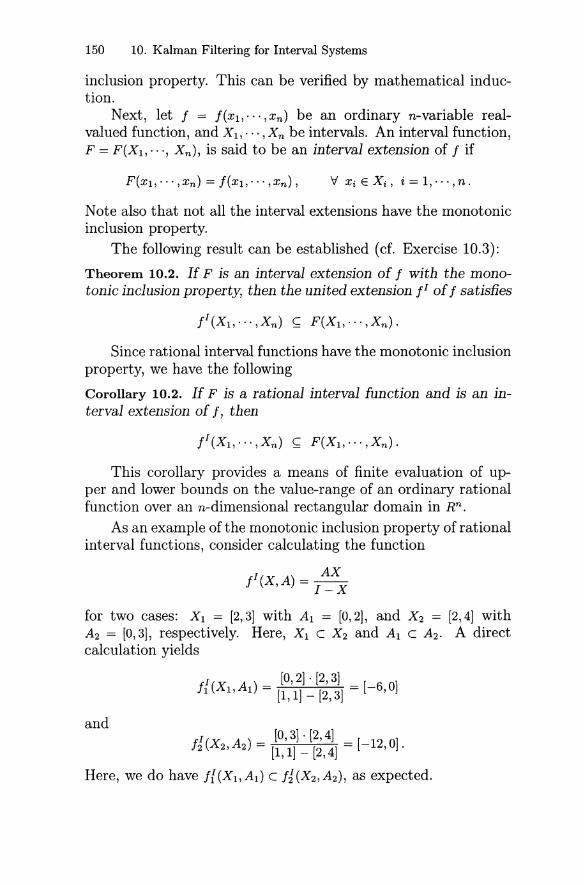
150 10. Kalman Filtering for Interval Systems
inclusion property. This can be verified by mathematical induction.
Next, let f = f(XI,··· ,xn ) be an ordinary n-variable realvalued function, and Xl,···, X n be intervals. An interval function,F = F(XI ,·· ., X n ), is said to be an interval extension of f if
V Xi E Xi, i = 1, ... , n .
Note also that not all the interval extensions have the monotonicinclusion property.
The following result can be established (cf. Exercise 10.3):
Theorem 10.2. If F is an interval extension of f with the monotonic inclusion property, then the united extension f1 of f satisfies
Since rational interval functions have the monotonic inclusionproperty, we have the following
Corollary 10.2. If F is a rational interval function and is an interval extension of f, then
This corollary provides a means of finite evaluation of upper and lower bounds on the value-range of an ordinary rationalfunction over an n-dimensional rectangular domain in Rn.
As an example of the monotonic inclusion property of rationalinterval functions, consider calculating the function
fI(X, A) = I~XX
for two cases: Xl = [2,3] with Al = [0,2], and X2 = [2,4] withA 2 = [0,3], respectively. Here, Xl C X 2 and Al C A 2 • A directcalculation yields
f 1(X A) = [0,2]· [2,3] = [-6 0]I I, I [1, 1] - [2,3] ,
and
f 1(X A) = [0,3]· [2,4] = [-12 0]2 2, 2 [1,1] - [2,4] ,.
Here, we do have ff (Xl, AI) C f1 (X2 , A2 ), as expected.
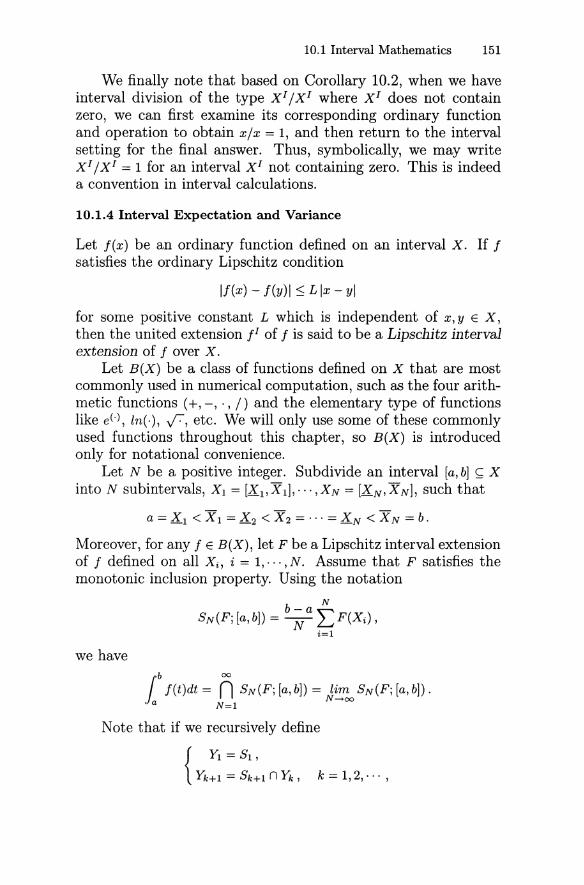
10.1 Interval Mathematics 151
We finally note that based on Corollary 10.2, when we haveinterval division of the type xIlxI where Xl does not containzero, we can first examine its corresponding ordinary functionand operation to obtain xix = 1, and then return to the intervalsetting for the final answer. Thus, symbolically, we may writeX I / X I = 1 for an interval X I not containing zero. This is indeeda convention in interval calculations.
10.1.4 Interval Expectation and Variance
Let I(x) be an ordinary function defined on an interval X. If Isatisfies the ordinary Lipschitz condition
II(x) - l(y)1 ::; L Ix - yl
for some positive constant L which is independent of x, y EX,then the united extension 11 of I is said to be a Lipscbitz intervalextension of lover X.
Let B(X) be a class of functions defined on X that are mostcommonly used in numerical computation, such as the four arithmetic functions (+, -, . , I) and the elementary type of functionslike e(o), In(·), V:-, etc. We will only use some of these commonlyused functions throughout this chapter, so B(X) is introducedonly for notational convenience.
Let N be a positive integer. Subdivide an interval [a, b] ~ Xinto N subintervals, Xl = [Xl,Xl],···,XN = [XN,XN], such that
a = Xl < Xl = X 2 < X 2 = ... = X N < XN = b.
Moreover, for any I E B(X), let F be a Lipschitz interval extensionof I defined on all Xi, i = 1,···, N. Assume that F satisfies themonotonic inclusion property. Using the notation
b-a NSN(F; [a, b]) = ~L F(Xi ) ,
i=l
we haveb CX)
1I(t)dt = nSN(F; [a, b]) = lim SN(F; [a, b]) .a N~CX)
N=l
Note that if we recursively define
{Yl = SI,
Yk+l = Sk+l n Yk , k = 1, 2, ... ,
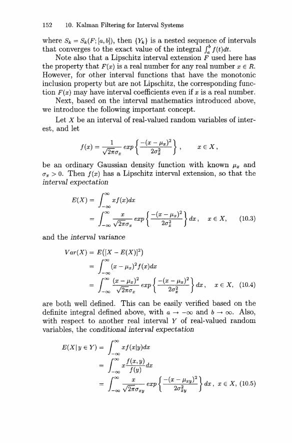
152 10. Kalman Filtering for Interval Systems
where Sk = Sk(F; [a, bD, then {Yk} is a nested sequence of intervalsthat converges to the exact value of the integral J: f(t)dt.
Note also that a Lipschitz interval extension F used here hasthe property that F(x) is a real number for any real number x E R.However, for other interval functions that have the monotonicinclusion property but are not Lipschitz, the corresponding function F(x) may have interval coefficients even if x is a real number.
Next, based on the interval mathematics introduced above,we introduce the following important concept.
Let X be an interval of real-valued random variables of interest, and let
1 { -(x - J.-tx)2 }f(x) = ~exp 2 2 '
y27rO"x O"XXEX,
be an ordinary Gaussian density function with known J.-tx ando"x > o. Then f(x) has a Lipschitz interval extension, so that theinterval expectation
E(X) = i: xf(x)dx
j CX) x { -(x - J.-tx)2 }= --exp 2 dx,-CX) ~O"x 20"x
and the interval variance
XEX, (10.3)
x E X, (10.4)
are both well defined. This can be easily verified based on thedefinite integral defined above, with a -+ -00 and b -+ 00. Also,with respect to another real interval Y of real-valued randomvariables, the conditional interval expectation
E(XI y E Y) = i: xf(xly)dx
j CX) f(x'Y)dx--x-CX) f(y)
j CX) x { -(x - J.-tXy)2 } dexp 2 x,
-ex:> ~O"xy 20"xyx E X, (10.5)
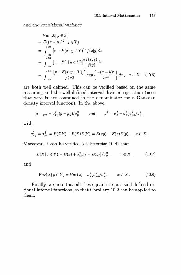
10.1 Interval Mathematics 153
and the conditional variance
Var(XI y E Y)
= E((x - JLx)21 y E Y)i: [x - E(xl Y E y)]2 f(xly)dx
jex:> [ J 2 !(x,y)
-00 x - E(xl y E Y) 7fij)dx
_ jex:> [x-E(xIYEy)]2 {_(X- ii)2}- rn=,- exp -2 dx,
-ex:> y21ra 2ax E X, (10.6)
are both well defined. This can be verified based on the samereasoning and the well-defined interval division operation (notethat zero is not contained in the denominator for a Gaussiandensity interval function). In the above,
and
with
a;y = a~x = E(XY) - E(X)E(Y) = E(xy) - E(x)E(y) , x EX.
Moreover, it can be verified (cf. Exercise 10.4) that
and
E(XI y E Y) = E(x) + a;y [y - E(y)]/a~, XEX,
xEX.
(10.7)
(10.8)
Finally, we note that all these quantities are well-defined rational interval functions, so that Corollary 10.2 can be applied tothem.
(10.10)
154 10. Kalman Filtering for Interval Systems
10.2 Interval Kalman Filtering
Now, return to the interval system (10.2). Observe that this system has an upper boundary system defined by all upper boundsof elements of its interval matrices:
and a lower boundary system using all lower bounds of the elements of its interval matrices:
{Xk+l = [Ak -1~Akl ]Xk + [rk -I~rkl ]~k'
Vk = [Ck -1~Ckl ]Xk +!1k·
We first point out that by performing the standard Kalman filtering algorithm for these two boundary systems, the resultingtwo filtering trajectories do not encompass all possible optimalsolutions of the interval system (10.2) (cf. Exercise 10.5). Asa matter of fact, there is no specific relation between these twoboundary trajectories and the entire family of optimal filteringsolutions: the two boundary trajectories and their neighboringones are generally intercrossing each other due to the noise perturbations. Therefore, a new filtering algorithm that can provideall-inclusive estimates for the interval system is needed. The interval Kalman filtering scheme derived below serves this purpose.
10.2.1 The Interval Kalman Filtering Scheme
Recall the derivation of the standard Kalman filtering algorithmgiven in Chapter 3, in which only matrix algebraic operations (additions, subtractions, multiplications, and inversions) and (conditional) expectations and variances are used. Since all theseoperations are well defined for interval matrices and rational interval functions, as discussed in the last section, the same derivation can be carried out for interval systems in exactly the sameway to yield a Kalman filtering algorithm for the interval system (10.2). This interval Kalman filtering algorithm is simplysummarized as follows:
10.2 Interval Kalman Filtering 155
The Interval Kalman Filtering Scheme
The main-process:
x& = E(x&),
xr = AL1XL1 + er [vr - ClAL1xL1] ,k = 1,2,··· . (10.11)
The co-process:
pt = Var(x&) ,
M£_l = A'-lPt-l [A'_l]T + Bk-lQk-l [Bk_l]T,
er = ML1 [Cl] T [[Cl]ML1 [cl] T + R k ] -1 ,
pt = [I-G'C£]M£_l[I-G,c£]T + [G']Rk[G,]T,k = 1,2, . .. . (10.12)
A comparison of this algorithm with the standard Kalmanfiltering scheme (3.25) reveals that they are exactly the same inform, except that all matrices and vectors in (10.11)-(10.12) areintervals. As a result, the interval estimate trajectory will divergerather quickly. However, this is due to the conservative intervalmodeling but not the new filtering algorithm.
It should be noted that from the theory this interval Kalmanfiltering algorithm is optimal for the interval system (10.2), inthe same sense as the standard Kalman filtering scheme, sinceno approximation is needed in its derivation. The filtering resultproduced by the interval Kalman filtering scheme is a sequenceof interval estimates, {x,}, that encompasses all possible optimal estimates {Xk} of the state vectors {Xk} which the intervalsystem may generate. Hence, the filtering result produced bythis interval Kalman filtering scheme is inclusive but generallyconservative in the sense that the range of interval estimates isoften unnecessarily wide in order to include all possible optimalsolutions.
It should also be remarked that just like the random vector(the measurement data) Vk in the ordinary case, the interval datavector v~ shown in the interval Kalman filtering scheme above isan uncertain interval vector before its realization (Le., before thedata actually being obtained), but will be an ordinary constantvector after it has been measured and obtained. This shouldavoid possible confusion in implementing the algorithm.
156 10. Kalman Filtering for Interval Systems
10.2.2 Suboptimal Interval Kalman Filter
To improve the computational efficiency, appropriate approximations of the interval Kalman filtering algorithm (10.11)-(10.12)may be applied. In this subsection, we suggest a suboptimal interval Kalman filtering scheme, by replacing its interval matrixinversion with its worst-case inversion, while keeping everythingelse unchanged.
To do so, let
and
where Ck is the center point of c£ and Mk-1 is center point ofM£_l (i.e., the nominal values of the interval matrices). Write
[[C1] Mk-l [cl] T + Rkr1
[T ]-1= [Ck + ~CkJ [Mk- 1+ ~Mk-1J [Ck + ~CkJ + Rk
= [CkMk-lCJ +~Rkrl,
where
~Rk = CkMk_1[~Ck]T + Ck[~Mk-1] C~ + Ck[~Mk-1] [~Ck]T
+ [~Ck]Mk-1C~ + [~Ck]Mk-1[~Ck]T + [~Ck] [~Mk-1]C~
+ [~Ck] [~Mk-1] [~Ck]T + Rk .
Then, in the algorithm (10.11)-(10.12), replace ~Rk by its upperbound matrix, I~Rkl, which consists of all the upper bounds ofthe interval elements of ~Rk = [[-rk(i,j), rk(i,j)]J, namely,
(10.13)
We should note that this I~Rkl is an ordinary (non-interval)matrix, so that when the ordinary inverse matrix [CkMk-1C~+I~Rkl] -1 is used to replace the interval matrix inverse [[C£J M£_l[Cl]T + R k ] -1, the matrix inversion becomes much easier. Moreimportantly, when the perturbation matrix ~Ck = 0 in (10.13),meaning that the measurement equation in system (10.2) is asaccurate as the nominal system model (10.1), we have I~Rkl = Rk.
Thus, by replacing ~Rk with I~Rkl, we obtain the followingsuboptimal interval Kalman filtering scheme.
10.2 Interval Kalman Filtering 157
A Suboptimal Interval Kalman Filtering Scheme
The main-process:
X5 = E(X5),-I AI -I GI [I CIAI -I JXk = k-lXk-l + k vk - k k-lXk-l ,
k = 1,2,··· .
The co-process:
pt = Var(x5),I I I [I JT I [ I JTM k - 1 = Ak-1Pk - 1 A k - 1 + Bk-1Qk-l B k - 1 ,
er = ML1 [Cl] T [CkMk-1CJ + I~Rkl] -1 ,
pt = [I-GkC£]M£_l[I-GkC£]T + [Gk]Rk[Gk]T,k = 1,2,··· .
(10.14)
(10.15)
Finally, we remark that the worst-case matrix I~Rkl givenin (10.13) contains the largest possible perturbations and is insome sense the "best" matrix that yields a numerically stableinverse. Another possible approximation is, if ~Ck is small, tosimply use I~Rkl ~ Rk. For some specific systems such as theradar tracking system to be discussed in the next subsection,special techniques are also possible to improve the speed and/oraccuracy in performing suboptimal interval filtering.
10.2.3 An Example of Target Tracking
In this subsection, we show a computer simulation by comparing the interval Kalman filtering with the standard one, fora simplified version of the radar tracking system (3.26), see also(4.22), (5.22), and (6.43),
(10.16)
where basic assumptions are the same as those stated for thesystem (10.2). Here, the system has uncertainty in an intervalentry:
hI = [h - ~h, h + ~h] = [0.01 - 0.001,0.01 + 0.001] = [0.009,0.011] ,
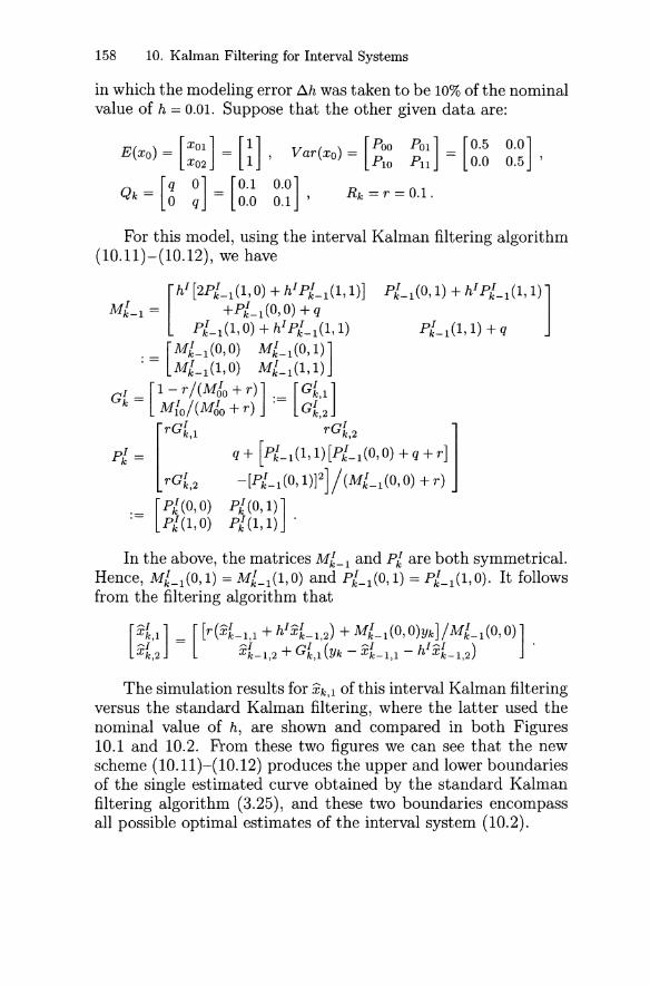
158 10. Kalman Filtering for Interval Systems
in which the modeling error ~h was taken to be 10% of the nominalvalue of h = 0.01. Suppose that the other given data are:
E(xo) = [XOl] = [1], Var(xo) = [POO POl] = [0.5 0.0]X02 1 PlO Pll 0.0 0.5 '
Qk = [6 ~] = [~:~ ~:n, Rk = r = 0.1.
For this model, using the interval Kalman filtering algorithm(10.11)-(10.12), we have
[
hI [2pI_ l (1,0) +hIpI_l(l,l)] pI- l (0, 1) + hIpI_l(l, 1)]M£-l = +pI-l (0,0) + q
pI-l (1,0) + hIpI-l (1,1) pI- l (1,1) + q
. = [M~_l(O,O) M~_l(O,l)]
. Mk_l (l,O) Mk_l (l,l)
Gl _[1-r/(M60+ r)]._ [Gk,l]k - I / I .- IM lO (Moo + r) Gk,2
[
rGk'l rGk,2 ]pt = q+ [PLl(l,l)[PLl(O,O)+q+r]
rG£,2 -[PLl(O, l)F]/(MLl(O,O) +r)
[pI (0,0) pI (0,1)]
.- pI (1,0) pI (1,1) .
In the above, the matrices M£_l and pI are both symmetrical.Hence, M£_l (0,1) = M£_l (1,0) and pI-l (0,1) = pI-l (1,0). It followsfrom the filtering algorithm that
[Xk'l] _ [ [r(xk-l,l + hIxk_l,2) + M£_l (0, O)Yk] / M£_l (0,0)]Xk,2 - Xk-1,2 + Gk,l (Yk - Xk-1,1 - hIxk_1,2) .
The simulation results for Xk,l of this interval Kalman filteringversus the standard Kalman filtering, where the latter used thenominal value of h, are shown and compared in both Figures10.1 and 10.2. From these two figures we can see that the newscheme (10.11)-(10.12) produces the upper and lower boundariesof the single estimated curve obtained by the standard Kalmanfiltering algorithm (3.25), and these two boundaries encompassall possible optimal estimates of the interval system (10.2).
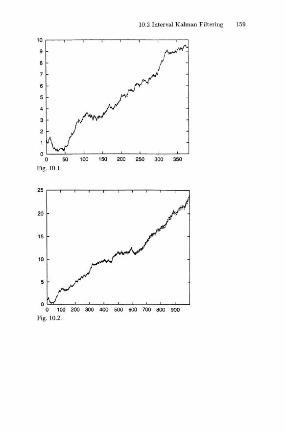
10.2 Interval Kalman Filtering 159
100 150 200 250 300 350
3
2
4
O'----'------I--~_---..I.--....a...-----...--...-......"
o 50
Fig. 10.1.
10 _-.......__-__--__----r---..,..--_,_--.,..--,
9
8
7
6
5
25 r------T---r-....,...-.....,...--,---..,.--r-----r----r--_
20
15
10
5
O---...----------------.-....---..I.-~o 100 200 300 400 500 600 700 800 900
Fig. 10.2.
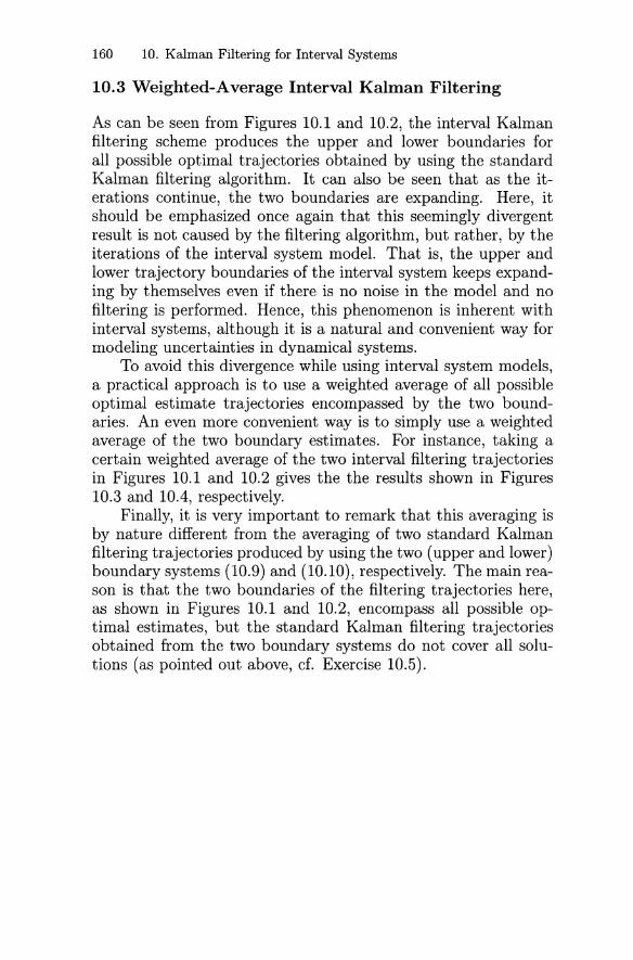
160 10. Kalman Filtering for Interval Systems
10.3 Weighted-Average Interval Kalman Filtering
As can be seen from Figures 10.1 and 10.2, the interval Kalmanfiltering scheme produces the upper and lower boundaries forall possible optimal trajectories obtained by using the standardKalman filtering algorithm. It can also be seen that as the iterations continue, the two boundaries are expanding. Here, itshould be emphasized once again that this seemingly divergentresult is not caused by the filtering algorithm, but rather, by theiterations of the interval system model. That is, the upper andlower trajectory boundaries of the interval system keeps expanding by themselves even if there is no noise in the model and nofiltering is performed. Hence, this phenomenon is inherent withinterval systems, although it is a natural and convenient way formodeling uncertainties in dynamical systems.
To avoid this divergence while using interval system models,a practical approach is to use a weighted average of all possibleoptimal estimate trajectories encompassed by the two boundaries. An even more convenient way is to simply use a weightedaverage of the two boundary estimates. For instance, taking acertain weighted average of the two interval filtering trajectoriesin Figures 10.1 and 10.2 gives the the results shown in Figures10.3 and 10.4, respectively.
Finally, it is very important to remark that this averaging isby nature different from the averaging of two standard Kalmanfiltering trajectories produced by using the two (upper and lower)boundary systems (10.9) and (10.10), respectively. The main reason is that the two boundaries of the filtering trajectories here,as shown in Figures 10.1 and 10.2, encompass all possible optimal estimates, but the standard Kalman filtering trajectoriesobtained from the two boundary systems do not cover all solutions (as pointed out above, cf. Exercise 10.5).
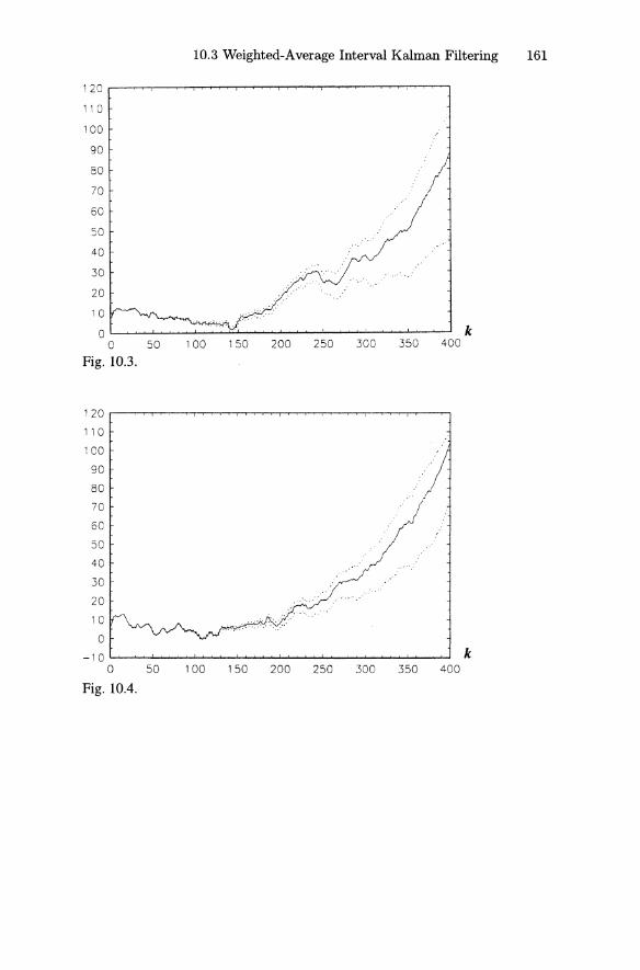
10.3 Weighted-Average Interval Kalman Filtering 161
120
110
100
90
80
70
60
50
40
30
20
10
0 k0 50 100 150 200 250 300 350 400
Fig. 10.3.
120
110
100
90
80
70
6C
50
40
30
20
10
0
-10 k0 50 100 150 200 250 300 350 400
Fig. 10.4.
162 10. Kalman Filtering for Interval Systems
Exercises
10.1. For three intervals x, Y, and Z, verify that
X+Y=Y+X,
Z + (X + Y) = (Z + X) + Y ,
XY=YX,
Z(XY) = (ZX)Y,
X + 0 = 0 + X = X and XO = OX = 0, where 0 = [0, 0] ,
XI=IX=X, where 1=[1,1],
Z(X + Y) ~ ZX + ZY, where = holds only if
(a) Z = [z,z];
(b)X=Y=O;
(c) xy 2:: 0 for all x E X and y E Y .
10.2. Let A, B, C be ordinary constant matrices and AI, B I , Cl beinterval matrices, respectively, of appropriate dimensions.Show that(a) AI ± B I = {A ± B IA E AI, B E B I };(b) AIB = {ABIA E AI};(c) AI+BI=BI+AI ;(d) AI+(BI+CI)=(AI+BI)+CI;(e) AI +O=O+AI =AI ;(f) All = IAI =AI ;(g) Subdistributive law:(g.l) (AI + BI)CI ~ AICI + BICI ;(g.2) Cl (AI + B I ) ~ ClAI + ClB I ;(h) (AI + BI)C = AIC + BIC;(i) C(AI + B I ) = CAI + CBI;(j) Associative and Subassociative laws:(j.1) AI(BC) ~ (AIB)C;(j.2) (ABI)CI ~ A(BI Cl) if Cl = -Cl;(j.3) A(BIC) = (ABI)C;(j.4) AI(BICI ) = (AIBI)CI , if B I = -BI and Cl = -Cl.
10.3. Prove Theorem 10.2.10.4. Verify formulas (10.7) and (10.8).10.5. Carry out a simple one-dimensional computer simulation to
show that by performing the standard Kalman filtering algorithm for the two boundary systems (10.9)-(10.10) of theinterval system (10.2), the two resulting filtering trajectories
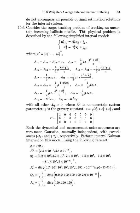
10.3 Weighted-Average Interval Kalman Filtering 163
do not encompass all possible optimal estimation solutionsfor the interval system.
10.6. Consider the target tracking problem of tracking an uncertain incoming ballistic missile. This physical problem isdescribed by the following simplified interval model:
{Xk+l = Akxk +{k'
1 Cl 1Vk = kXk + '!lk'
1 z2 + x~All = A 22 = A 33 = 1, A 44 = -- gX7 ---
2 z1 X7X4X5 1 X7X4X6
A 45 = A 54 = - - 9-- , A 46 = A 64 = - - 9-- ,2 z 2 z
1 1 z2 + xgA 47 = -"2 gX4 z , A 55 = -"2 gX7 z
1 X7X5X6 1A56=A65=-"2g-z-' A57=-"2gx5z,
1 z2 + x~ 1A 66 = -- gX7 A67 = -- gX6 Z ,
2 z 2A 76 = -Klx7, A 77 = - Klx6,
with all other A ij = 0, where K l is an uncertain systemparameter, 9 is the gravety constant, z = v'x~ + xg + x~, and
[
1 0 0 0 0 0 0]C= 0 1 0 0 0 0 0 .
o 0 1 000 0
Both the dynamical and measurement noise sequences arezero-mean Gaussian, mutually independent, with covariances {Qk} and {Rk}, respectively. Perform interval Kalmanfiltering on this model, using the following data set:
9 = 0.981,
K 1 = [2.3 X 10⁻⁵ ,3.5 x 10-5J '
x~ = [3.2 x 10⁵ ,3.2 x 105 ,2.1 x 105 ,-1.5 x 10⁴ ,-1.5 x 10⁴,
- 8.1 X 10³ ,5 x 10- l0JT ,
pt = diag{ 106, 106
, 106 ,106, 106
, 1.286 x 1O- 13exp{ -23.616} } ,
Qk = _1_ diag{O, 0, 0,100,100,100,2.0 x 10- l8} ,
k+1
Rk = k: 1 diag{ 150, 150, 150} .
11. Wavelet Kalman Filtering
In addition to the Kalman filtering algorithms discussed in theprevious chapters, there are other computational schemes available for digital filtering performed in the time domain. Amongthem, perhaps the most exciting ones are wavelet algorithms,which are useful tools for multichannel signal processing (e.g.,estimation or filtering) and multiresolution signal analysis. Thischapter is devoted to introduce this effective technique of waveletKalman filtering by means of a specific application for illustration- simultaneous estimation and decomposition of random signalsvia a filter-bank-based Kalman filtering approach using wavelets.
11.1 Wavelet Preliminaries
The notion of wavelets was first introduced in the earlier 1980's,as a family of functions generated by a single function, calledthe "basic wavelet," by two simple operations: translation andscaling. Let 'ljJ(t) be such a basic wavelet. Then, with a scalingconstant, a, and a translation constant, b, we obtain a family ofwavelets of the form 'ljJ((t - b)/a). Using this family of waveletsas the integral kernel to define an integral transform, called theintegral wavelet transform (IWT):
(W",f) (b, a) = lal- 1/
21: f(t) 'l/J( (t - b)ja)) dt, f E £2 , (11.1)
we can analyze the functions (or signals) f (t) at different positions and at different scales according to the values of a and b.Note that the wavelet 'ljJ(t) acts as a time-window function whose"width" narrows as the value of the "scale" a in (11.1) decreases.Hence, if the frequency, w in its Fourier transform :(f(w), is definedto be inversely proportional to the scale a, then the width of thetime window induced by 'ljJ(t) narrows for studying high-frequencyobjects and widens for observing low-frequency situations. Inaddition, if the basic wavelet 'ljJ(t) is so chosen that its Fouriertransform is also a window function, then the IWT, (W1/Jf) (b, a),can be used for time-frequency localization and analysis of f(t)around t == b on a frequency band defined by the scale a.
11.1 Wavelet Preliminaries 165
11.1.1 Wavelet Fundamentals
An elegant approach to studying wavelets is via "multiresolutionanalysis." Let £2 denote the space of real-valued finite-energyfunctions in the continuous-time domain (-00, (0), in which theinner product is defined by (/,g) = f~oo I(t)g(t) dt and the normis defined by 11/11£2 '= Ji(7J)i. A nested sequence {Vk} of closedsubspaces of £2 is said to form a multiresolution analysis of £2 ifthere exists some window function (cf. Exercise 11.1), cjJ(t) E £2,which satisfies the following properties:
(i) for each integer k, the set
J. - ... -1 0 1 ... }- , '"
is an unconditional basis of Vk, namely, its linear span isdense in Vk and for each k,
alI{cj}II;2 :S 11 jJ;oo CjePkj 1[2 :S fJll{cj}II;2 (11.2)
for all {Cj} E £2, where II{cj}lll 2= V'L-'J=-oo ICjI2;(ii) the union of Vk is dense in £2;(iii) the intersection of all Vk'S is the zero function; and(iv) f(t) E Vk if and only if 1(2t) E Vk+l.
Let Wk be the orthogonal complementary subspace of Vk+lrelative to Vk, and we use the notation
(11.3)
Then it is clear that Wk .l W n for all k =1= n, and the entire space£2 is an orthogonal sum of the spaces Wk, namely:
(11.4)
Suppose that there is a function, 1jJ(t) E Wo, such that both 1jJ(t)and its Fourier transform ;j(w) have sufficiently fast decay at ±oo(cf. Exercise 11.2), and that for each integer k,
Jo - ••• -1 0 1 ... }- , '" (11.5)
i,j=···,-l,O,l,··· .
166 11. Wavelet Kalman Filtering
is an unconditional basis of Wk. Then 'ljJ(t) is called a wavelet (cf.Exercise 11.3). Let :;fi(t) E Wo be the dual of 'ljJ(t) , in the sense that
I: ~(t - i) 1jJ(t - j) dt = Oij ,
Then both :;fi(t) and :;fi(w) are window functions, in the time andfrequency domains, respectively. If ;j(t) is used as a basic waveletin the definition of the IWT, then real-time algorithms are available to determine (W~f)(b,a) at the dyadic time instants b = j /2k
on the kth frequency bands defined by the scale a = 2- k • Also, f(t)can be reconstructed in real-time from information of (W~f)(b, a)
at these dyadic data values.More precisely, by defining
k/2 k'ljJkj(t) = 2 'ljJ(2 t - j) ,
any function f(t) E £2 can be expressed as a wavelet series
00 00
f(t) = L: L: dJ'ljJk,j(t)k=-ooj=-oo
with
(11.6)
(11.7)
dJ = (W~f) (j2- k, 2- k
) . (11.8)
According to (11.3), there exist two sequences {aj} and {bj} in £2
such that00
q;(2t -f) = L: [at-2jq;(t - j) + bt- 2j 'ljJ(t - j)J (11.9)j=-oo
for all integers £; and it follows from property (i) and (11.3) thattwo sequences {Pj} and {qj} in £2 are uniquely determined suchthat
00
and
q;(t) = L: Pj q;(2t - j)j=-oo
00
'ljJ(t) = L: qj c/J(2t - j) .j=-oo
(11.10)
(11.11)
The pair of sequences ({aj}, {bj }) yields a pyramid algorithm forfinding the IWT values {dj}; while the pair of sequences ({Pj}, {qj})
11.1 Wavelet Preliminaries 167
yields a pyramid algorithm for reconstructing f(t) from the IWTvalues {dj}.
We remark that if cjJ(t) is chosen as a B-spline function, thena compactly supported wavelet 'ljJ(t) is obtained such that its dual;j;(t) has exponential decay at ±oo and the IWT with respect to;j;(t) has linear phase. Moreover, both sequences {Pj} and {qj}are finite, while {aj} and {bj} have very fast exponential decay.It should be noted that the spline wavelets 'ljJ(t) and ;j;(t) haveexplicit formulations and can be easily implemented.
11.1.2 Discrete Wavelet Transform and Filter Banks
For a given sequence of scalar deterministic signals, {x( i, n)} E
£2, at a fixed resolution level i, a lower resolution signal can bederived by lowpass filtering with a halfband lowpass filter havingan impulse response {h(n)}. More precisely, a sequence of thelower resolution signal (indicated by an index L) is obtained bydownsampling the output of the lowpass filter by two, namely,h(n) ~ h(2n), so that
00
xL(i - 1, n) = L: h(2n - k) x(i, k) .k=-oo
(11.12)
Here, (11.12) defines a mapping from £2 to itself. The waveletcoefficients, as a complement to xL(i - 1, n), will be denoted by{xH(i-1,n)}, which can be computed by first using a highpass filter with an impulse response {g(n)} and then using downsamplingthe output of the highpass filtering by two. This yields
00
xH(i - 1, n) = L: g(2n - k) x(i, k).k=-oo
(11.13)
The original signal {x( i, n)} can be recovered from the two filtered and downsampled (lower resolution) signals {xL(i-1,n)} and{xH(i-1, n)}. Filters {h(n)} and {g(n)} must meet some constraintsin order to produce a perfect reconstruction for the signal. Themost important constraint is that the filter impulse responsesform an orthonormal set. For this reason, (11.12) and (11.13) together can be considered as a decomposition of the original signalonto an orthonormal basis, and the reconstruction
00
x(i, n) = L: h(2k - n)xL(i - 1, k)k=-oo
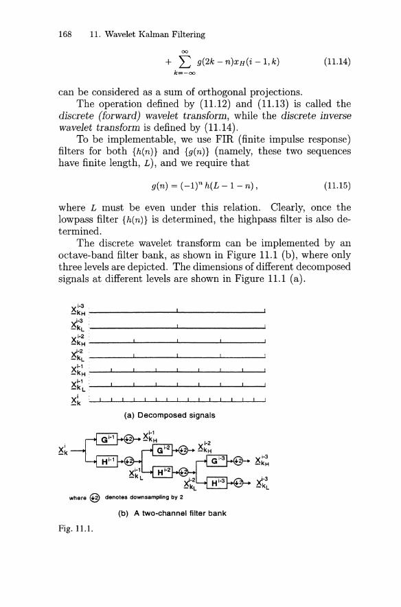
168 11. Wavelet Kalman Filtering
00
+ L g(2k - n)xH(i - 1, k)k=-oo
(11.14)
can be considered as a sum of orthogonal projections.The operation defined by (11.12) and (11.13) is called the
discrete (forward) wavelet transform, while the discrete inversewavelet transform is defined by (11.14).
To be implementable, we use FIR (finite impulse response)filters for both {h(n)} and {g(n)} (namely, these two sequenceshave finite length, L), and we require that
g(n) = (_1)n h(L - 1 - n) , (11.15)
where L must be even under this relation. Clearly, once thelowpass filter {h(n)} is determined, the highpass filter is also determined.
The discrete wavelet transform can be implemented by anoctave-band filter bank, as shown in Figure 11.1 (b), where onlythree levels are depicted. The dimensions of different decomposedsignals at different levels are shown in Figure 11.1 (a) .
Xi-3 .
-kH '-:---------------~~-3 :-kL : ----'- --...i
2S~~ _:---~--------"'-----~Xi-2 :-kL :,-__--....L -..... --'-- ~
Xi-1 :_ kH :'----a_--....L_---r._-....._--'--_--'--_~_.....
X i-1 :-k L ._---I_--....L_---r._-....._--'--_--'--_~_....&
X i :--''----I'----I'----I----.Io---r.----'---'-__--'---''''--oI.--'''- ~I__..1_k
(a) Decomposed signals
+)(-2-kL
where @ denotes downsampling by 2
X i-3-kH
(b) A two-channel filter bank
Fig. 11.1.
11.1 Wavelet Preliminaries 169
For a sequence of deterministic signals with finite length, it ismore convenient to describe the wavelet transform in an operatorform. Consider a sequence of signals at resolution level i withlength M:
X1 = [x(i, k - M + 1), x(i, k - M + 2)" .. ,x(i, k)] T .
Formulas (11.12) and (11.13) can be written in the following operator form:
and
where operators H i - 1 and G i - 1 are composed of lowpass and highpass filter responses [the {h(n)} and {g(n)} in (11.12) and (11.13)],mapping from level i to level i -1. Similarly, when mapping fromlevel i-I to level i, (11.14) can be written in operator form as(cf. Exercise 11.4)
(11.16)
where
On the other hand, the orthogonality constraint can also be expressed in operator form as
(Hi-1)THi- 1+ (Gi-1)T G i- 1 = 1
and
[Hi-1(Hi-1)T Hi-l(Gi-l)T] _ [I 0]Gi-1(Hi-l)T Gi-l(Gi-l)T - 0 1 .
A simultaneous multilevel signal decomposition can be carried out by a filter bank. For instance, to decompose x1 intothree levels, as shown in Figure 11.1, the following compositetransform can be applied:
X i - 3-kLX i - 3
-kH = T i - 3 li XiXi-2 -k'-kHX i - 1-kH
[
Hi-3Hi-2Hi_l].. Gi-3Hi-2Hi-l
T~-31~ -- G i - 2H i - 1
G i - 1
is an orthogonal matrix, simultaneously mapping X1 onto thethree levels of the filter bank.
170 11. Wavelet Kalman Filtering
11.2 Singal Estimation and Decomposition
In random signal estimation and decomposition, a general approach is first to estimate the unknown signal using its measurement data and then to decompose the estimated signal accordingto the resolution requirement. Such a two-step approach is offline in nature and is often not desirable for real-time applications.
In this section, a technique for simultaneous optimal estimation and multiresolutional decomposition of a random signal is developed. This is used as an example for illustratingwavelet Kalman filtering. An algorithm that simultaneously performs estimation and decomposition is derived based on the discrete wavelet transform and is implemented by a Kalman filterbank. The algorithm preserves the merits of the Kalman filteringscheme for estimation, in the sense that it produces an optimal(linear, unbiased, and minimum error-variance) estimate of theunknown signal, in a recursive manner using sampling data obtained from the noisy signal.
The approach to be developed has the following special features: First, instead of a two-step approach, it determines inone step the estimated signal such that the resulting signal naturally possesses the desired decomposition. Second, the recursiveKalman filtering scheme is employed in the algorithm, so as toachieve the estimation and decomposition of the unknown butnoisy signal, not only simultaneously but also optimally. Finally,the entire signal processing is performed on-line, which is a realtime process in the sense that as a block of new measurementsflows in, a block of estimates of the signal flows out in the requireddecomposition form. In this procedure, the signal is first dividedinto blocks and then filtering is performed over data blocks. Tothis end, the current estimates are obtained based on a blockof current measurements and the previous block of optimal estimates. Here, the length of the data block is determined by thenumber of levels of the desired decomposition. An octave-bandfilter bank is employed as an effective vehicle for the multiresolutional decomposition.
11.2.1 Estimation and Decomposition of Random Signals
Now, consider a sequence of one-dimensional random signals,{x(N, k)} at the highest resolution level (level N), governed by
x(N, k + 1) = A(N, k)x(N, k) + ~(N, k) , (11.17)
11.2 Singal Estimation and Decomposition 171
with measurement
v(N, k) = C(N, k)x(N, k) + 1J(N, k) , (11.18)
where {~(N, k)} and {1J(N, k)} are mutually independent Gaussiannoise sequences with zero mean and variances Q(N, k) and R(N, k),respectively.
Given a sequence of measurements, {v(N, k)}, the conventional way of estimation and decomposition of the random signal{X(N, k)} is performed in a sequential manner: first, find an estimation x(N, k) at the highest resolutional level; then apply awavelet transform to decompose it into different resolutions.
In the following, an algorithm for simultaneous estimationand decomposition of the random signal is derived. For simplicity, only two-level decomposition and estimation will be discussed, i.e., from level N to levels N - 1 and N - 2. At all otherlevels, simultaneous estimation and decomposition procedures areexactly the same.
A data block with length M = 22 = 4 is chosen, where base 2is used in order to design an octave filter bank, and power 2 isthe same as the number of the levels in the decomposition. Upto instant k, we have
X~ = [x(N, k - 3), x(N, k - 2), x(N, k - 1), x(N, k)] T ,
for which the equivalent dynamical system in a data-block formis derived as follows. For notional convenience, the system andmeasurement equations, (11.17) and (11.18), are assumed to betime-invariant, and the level index N is dropped. The propagation is carried out over an interval of length M, yielding
or
or
x(N, k + 1) = Ax(N, k) + ~(N, k) ,
x(N, k + 1) = A2x(N, k - 1) + A~(N, k - 1) + ~(N, k) ,
x(N, k + 1) =A3x(N, k - 2) + A2~(N, k - 2)
+ A~(N, k -1) + ~(N, k),
(11.19)
(11.20)
(11.21)
172 11. Wavelet Kalman Filtering
or
x(N, k + 1) =A4x(N, k - 3) + A3~(N, k - 3) + A2~(N, k - 2)
+ A~(N, k - 1) + ~(N, k). (11.22)
Taking the average of (11.19), (11.20), (11.21) and (11.22), weobtain
1 1x(N, k + 1) =4 A4x(N, k - 3) + 4A3x(N, k - 2)
1 1+ 4A2x(N, k - 1) + 4Ax(N, k) + ~(1),
where
~(1) =~ A3~(N, k - 3) + ~A2~(N, k - 2)
3+4A~(N,k-l)+~(N,k). (11.23)
Also, taking into account all propagations, we finally have a dynamical system in a data-block form as follows (cf. Exercise11.5):
[
X(N'k+l)] [iA4 !A3 !A2
!A]x(N,k+2) _ 0 tA4 l A3 14A2x(N,k+3) - 0 0 IA4 IA3x(N,k+4) 0 0 0 A4
'---v-'" " v
Kf:+l A
x [~1zj=~l] + [~m] , (11.24)
x(N,k) ~(4)'---v-'" '--v--"
Kf: wr:where ~(i), i = 2,3,4, are similarly defiend, with
E{W:} = 0 and E{W: (W:) T} = Q,
and the elements of Q are given by1 6 1 4 9 2 _ 1 5 1 3
Qll = 16 A Q + 4 A Q + 16 A Q + Q , q12 = (3 A Q + "2 A Q + AQ ,
3 4 2 3Q13 = 8A Q + A Q, Q14 = A Q, Q21 = Q12 ,
1 6 4 4 2 - 1 5 3Q22 = 9" A Q + 9" A Q + A Q + Q , q23 = 3A Q + A Q + AQ ,
q24 = A4Q + A2Q, q31 = q13, q32 = q23 ,
1 6 4 2 5 3q33 = 4A Q + A Q + A Q + Q , Q34 = A Q + A Q + AQ ,
q41 = q14 , q42 = q24, q43 = q34, q44 = A6 Q + A4Q + A2Q + Q.
11.2 Singal Estimation and Decomposition 173
The measurement equation associated with (11.24) can beeasily constructed as
where
E{nf} = 0 and E{nf (nf) T} = R = diag {R, R, R, R}.
Two-level decomposition is then performed, leading to
[XN
-
2
]k HN-2H N- 1
X If- 2 = [GN-2H N-l] X N = T N - 2IN X N.-kH -k-k
X N - 1 GN-l-kH
Substituting (11.25) into (11.24) results in
(11.25)
(11.26)
where
wf = TN- 2INW:, E{wf} = 0, E{wf (wf) T} = Q,
A = T N- 2INA(TN- 2IN)T , Q = TN-2INQ(TN-2IN)T .
Equation (11.26) describes a dynamical system for the decomposed quantities. Its associated measurement equation can alsobe derived by substituting (11.25) into (11.24), yielding
(11.27)
wherec = C(TN - 2IN ) T .
Now, we have obtained the system and measurement equations, (11.26) and (11.27), for the decomposed quantities. Thenext task is to estimate these quantities using measurement data.The Kalman filter is readily applied to (11.26) and (11.27) to provide optimal estimates for these decomposed quantities.
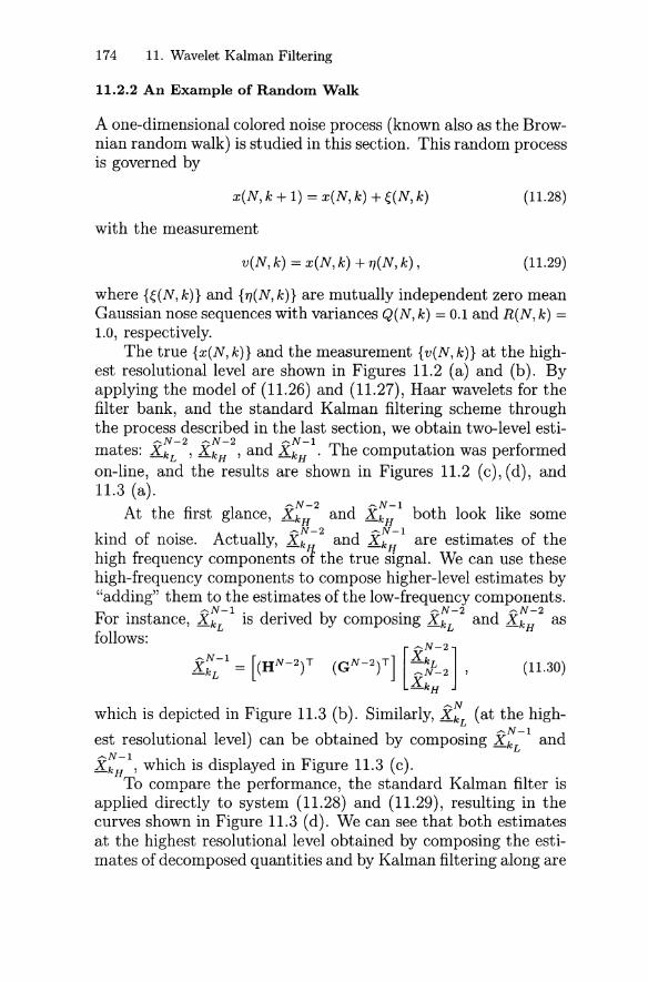
174 11. Wavelet Kalman Filtering
11.2.2 An Example of Random Walk
A one-dimensional colored noise process (known also as the Brownian random walk) is studied in this section. This random processis governed by
x(N, k + 1) = x(N, k) + ~(N, k)
with the measurement
v(N, k) = x(N, k) + TJ(N, k),
(11.28)
(11.29)
where {~(N, k)} and {TJ(N, k)} are mutually independent zero meanGaussian nose sequences with variances Q(N, k) = 0.1 and R(N, k) =1.0, respectively.
The true {x(N,k)} and the measurement {v(N,k)} at the highest resolutionallevel are shown in Figures 11.2 (a) and (b). Byapplying the model of (11.26) and (11.27), Haar wavelets for thefilter bank, and the standard Kalman filtering scheme throughthe process described in the last section, we obtain two-level esti-
-N-2 -N-2 -N-1 .mates: X kL ,XkH ,and X kH . The computatIon was performedon-line, and the results are shown in Figures 11.2 (c), (d), and11.3 (a).
-N-2 -N-1At the first glance, X kH and X kH both look like some
-N-2 -N-1kind of noise. Actually, X k and X kH are estimates of thehigh frequency components 01 the true signal. We can use thesehigh-frequency components to compose higher-level estimates by"adding" them to the estimates of the low-frequency components.
-N-1 -N-2 -N-2For instance, X kL is derived by composing X kL and X kH asfollows: -N-2
X:£-1 = [(HN- 2)T (GN- 2)T] [~~-2] , (11.30)X kH
which is depicted in Figure 11.3 (b). Similarly, x:£ (at the high
est resolutional level) can be obtained by composing X:£-1 and
x:;;\ which is displayed in Figure 11.3 (c).To compare the performance, the standard Kalman filter is
applied directly to system (11.28) and (11.29), resulting in thecurves shown in Figure 11.3 (d). We can see that both estimatesat the highest resolutional level obtained by composing the estimates of decomposed quantities and by Kalman filtering along are
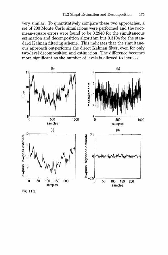
11.2 Singal Estimation and Decomposition 175
very similar. To quantitatively compare these two approaches, aset of 200 Monte Carlo simulations were performed and the rootmean-square errors were found to be 0.2940 for the simultaneousestimation and decomposition algorithm but 0.3104 for the standard Kalman filtering scheme. This illdicates that the simultaneous approach outperforms the direct Kalman filter, even for onlytwo-level decomposition and estimation. The difference becomesmore significant as the number of levels is allowed to increase.
1000500samples
(d)
50 100 150 200samples
~ 12c:Q)
E~ 10:J(/)«SQ)
E 8
(b)14r--------r-------,
Q) 0.5 r-----,.----r-----,---..,..----,
caE
:;::;(/)Q)
(/)(/)euB- 00)
:cI
(/)(/)
eua.~
.Q -0.5 '-------L_--'-_--1-_----L-_--l
o
1000500samples
(c)
50 100 150 200samples
8'---------'-----~o
10
11,.------r------.....
9
(a)
Q) 12 .-----,.---r---r--~-__.10E~ 11Q)
(/)(/)
ctS~10oI~ 9ctSa.~
.Q 8~~---'-_---'-_---L-_-.Jo
Fig. 11.2.
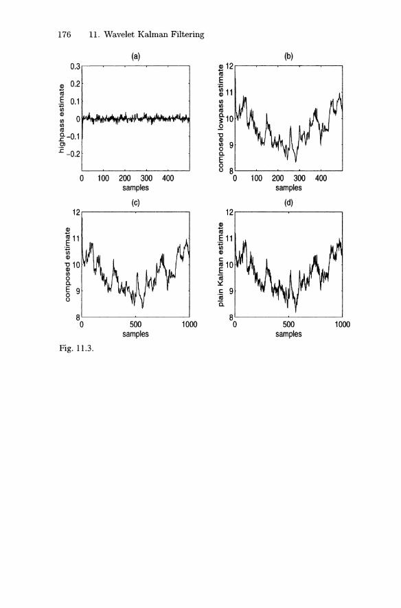
176 11. Wavelet Kalman Filtering
(a) (b)0.3 Cl) 12...,
(U
0.2 EQ)
~ 11caE 0.1 en~ en
(UCl)
0 ~10fI)f/J .QctSf-0.1 -0
0> ~ 9:E -0.2 0a.
E00 8
0 100 200 300 400 0 100 200 300 400samples samples
(c) (d)12 12
Cl)Cl) caca 11 E11E ~~ Cl)Q) c:-g 10 ctS10
EfI)(ij0a. ~
E 9 .£ 90(J (U
a.80 500 1000 500 1000
samples samples
Fig. 11.3.
11.2 Singal Estimation and Decomposition 177
Exercises
11.1. The following Haar and triangle functions are typical window functions in the time domain:
4JH(t) = { ~
4JT(t) = { 2 - ~
O::;t<l
otherwise;
O::;t<l,
1::;t<2,
otherwise.
and
Sketch these two functions, and verify that
Here, cPH(t) and cPT(t) are also called B-splines of degree zeroand one, respectively. B-spline of degree n can be generatedvia
4Jn(t) =11
4Jn-1(t - r)dr, n = 2,3" ...
Calculate and sketch cP2(t) and cP3(t). (Note that cPo == cPHand cPl == cPT.)
11.2. Find the Fourier transforms of cPH(t) and cPT(t) definedabove.
11.3. Based on the graphs of cPH(t) and cPT(t), sketch
Moreover, sketch the wavelets
1 1VJT(t) == -2 cPT(2t) - 2<PT(2t -2) + cPT(2t - 1) .
11.4. Verify (11.16).11.5. Verify (11.24) and (11.26).
12. Notes
The objective of this monograph has been to give a rigorous andyet elementary treatment of the Kalman filter theory and brieflyintroduce some of its real-time applications. No attempt wasmade to cover all the rudiment of the theory, and only a smallsample of its applications has been included. There are manytexts in the literature that were written for different purposes,including Anderson and Moore (1979), Balakrishnan (1984,87),Brammer and Siffiin (1989), Catlin (1989), Chen (1985), Chen,Chen and Hsu (1995), Goodwin and Sin (1984), Haykin (1986),Lewis (1986), Mendel (1987), Ruymgaart and Soong (1985,89),Sorenson (1985), Stengel (1986), and Young (1984). Unfortunately, in our detailed treatment we have had to omit manyimportant topics; some of these will be introduced very brieflyin this chapter. The interested reader is referred to the modestbibliography in this text for further study.
12.1 The Kalman Smoother
Suppose that data information is available over a discrete-timetime-interval {I, 2,··· ,N}. For any K with 1 ::; K < N, the optimalestimate xKIN of the state vector XK using all the data informationon this time-interval (i.e. past, present, and future informationare being used) is called a (digital) smoothing estimate of XK (cf.Definition 2.1 in Chapter 2). Although this smoothing problem issomewhat different from the real-time estimation which we considered in this text, it still has many useful applications. Onesuch application is satellite orbit determination, where the satellite orbit estimation is allowed to be made after a certain periodof time. More precisely, consider the following linear deterministic/stochastic system with a fixed terminal time N:
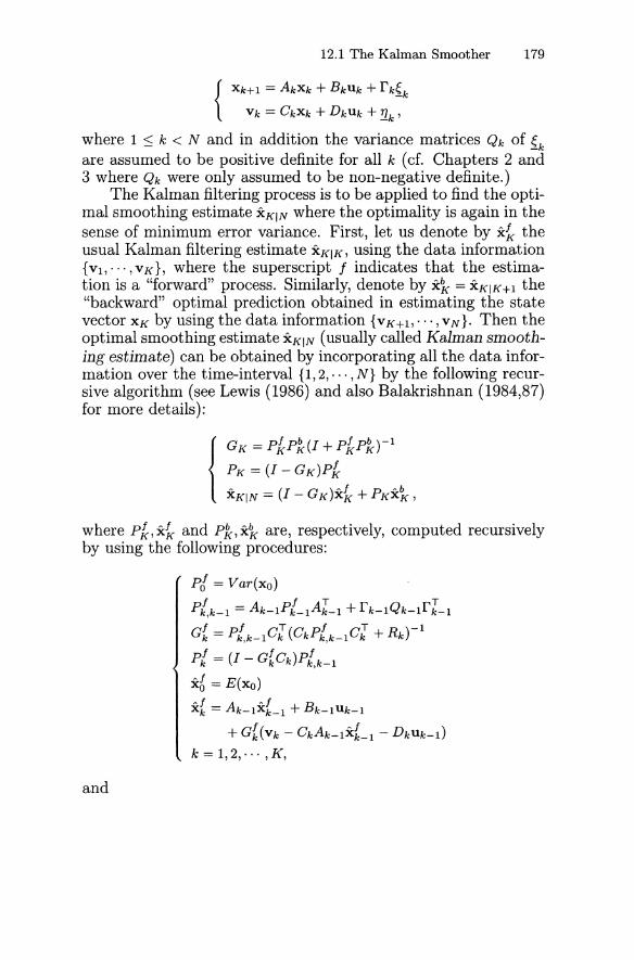
12.1 The Kalman Smoother 179
{
Xk+1 = AkXk + BkUk + rk~k
Vk = CkXk + DkUk + '!lk '
where 1 :::; k < N and in addition the variance matrices Qk of 5.k
are assumed to be positive definite for all k (cf. Chapters 2 and3 where Qk were only assumed to be non-negative definite.)
The Kalman filtering process is to be applied to find the optimal smoothing estimate xKIN where the optimality is again in thesense of minimum error variance. First, let us denote by x:f< theusual Kalman filtering estimate xKIK, using the data information{VI,···, VK}, where the superscript f indicates that the estimation is a "forward" process. Similarly, denote by x'K = xKIK+I the"backward" optimal prediction obtained in estimating the statevector XK by using the data information {VK+I,···, VN}. Then theoptimal smoothing estimate xKIN (usually called Kalman smoothing estimate) can be obtained by incorporating all the data information over the time-interval {I, 2,· .. , N} by the following recursive algorithm (see Lewis (1986) and also Balakrishnan (1984,87)for more details):
{
GK=pkpk(1+pkpk)-1
PK = (1 - GK)pk
xKIN = (1 - GK)xk + PKx'K,
where pk, x:f< and Pk, x'K are, respectively, computed recursivelyby using the following procedures:
pt = Var(xo)
P[k-I = Ak-IP{_IAl- I + rk-IQk-Irl-1
G' = P[k-ICl (CkP!,k_lCl + Rk)-l
pt = (1 - G'Ck)P!,k_l
x6 = E(xo)
x, = Ak-IX'_I + Bk-lUk-l
+ G'(Vk - CkAk-lX'_l - DkUk-l)
k = 1,2,··· ,K,
and
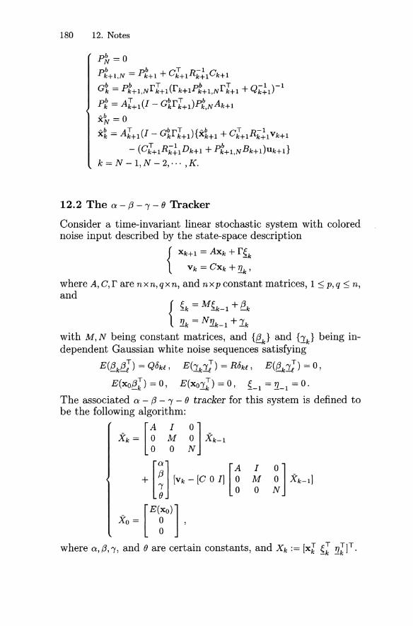
180 12. Notes
PJv == 0
P:+1,N == P:+1 + cl+1Rk~lCk+l
G~ == p:+l,Nr~+l(rk+lP:+l,Nr~+l + Qk~l)-l
P: == Al+1(1 - G~rl+l)P:,NAk+l"b 0XN ==" b AT (I Gb rT ) { " b CT R- 1Xk == k+l - k k+l Xk+l + k+l k+l Vk+l
- (Cl+lRk~lDk+l + P:+1,NBk+l)Uk+l}k == N - 1, N - 2, ... ,K.
12.2 The a - {3 -, - () Tracker
Consider a time-invariant linear stochastic system with colorednoise input described by the state-space description
{Xk+l == AXk + r~k
Vk == CXk + !lk '
where A, C, rare n x n, q x n, and n x p constant matrices, 1 ::; p, q ::; n,and
{~k: M~k_l +~!lk - N!lk_l + lk
with M, N being constant matrices, and {~k} and {lk} being independent Gaussian white noise sequences satisfying
E(~k[[J) == Q8kl , E(lkL) == R8kl , E(~kL) == 0,
E(xofi;) == 0, E(xOl~) == 0, ~-l == !l-l == o.The associated a - (3 - , - () tracker for this system is defined tobe the following algorithm:
Xk == [~ ~ ~ ] Xk-lo 0 N
+ [~] [Vk - [e 0 I] [~ ~ 1]Xk-l]
Xo = [E!O)] ,
where a, {3", and () are certain constants, and Xk :== [xl ~; !l~]T.
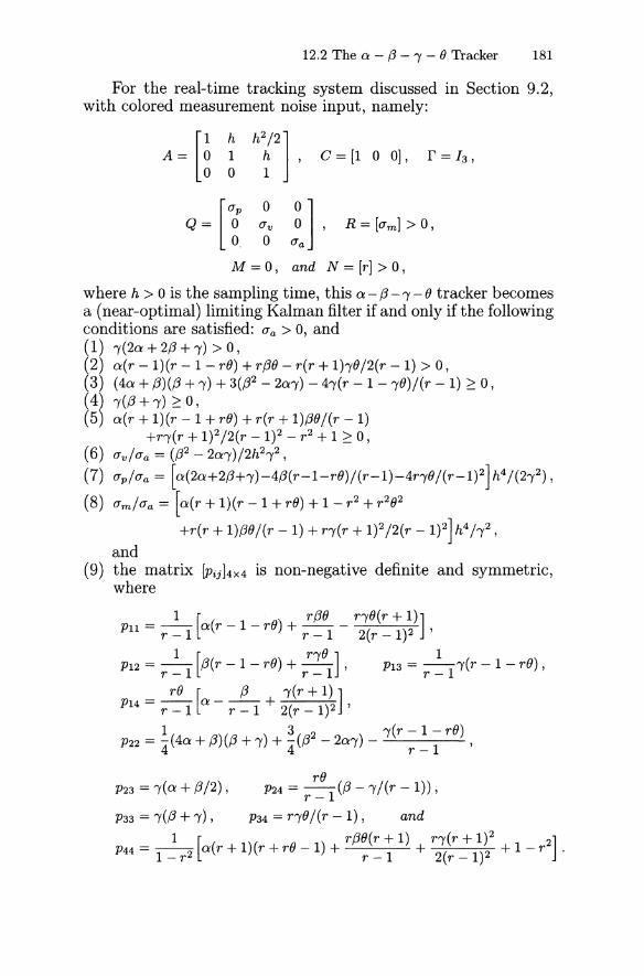
12.2 The a - {3 - , - () Tracker 181
For the real-time tracking system discussed in Section 9.2,with colored measurement noise input, namely:
A= [~ ~ h~2], C= [1 0 0], r = 13 ,
o 0 1
lap 0 0 ]
Q = 0 av 0 , R = [am] > 0,o. 0 aa
M = 0 , and N = [r] > 0 ,
where h > 0 is the sampling time, this a - {3 -, - () tracker becomesa (near-optimal) limiting Kalman filter if and only if the followingconditions are satisfied: aa > 0, and(1) ,(2a+2{3+,) >0,(2) a(r - 1)(r - 1 - r()) + r{3() - r(r + 1),()/2(r - 1) > 0,(3) (4a + {3)({3 +,) + 3({32 - 2a,) - 4,(r - 1 - ,())/(r - 1) ~ 0,(4) ,({3+,) ~O,(5) a(r + 1)(r - 1 + r()) + r(r + 1){3() j(r - 1)
+r,(r + 1)2 j2(r - 1)2 - r 2 + 1 ~ 0,(6) av/aa = ({32 - 2a,)j2h2,2,
(7) ap/aa = [a(2a+2,6+'Y)-4,6(r-1-rB)/(r-1)-4QB/(r-1)2] h4 /(2'Y2) ,
(8) am/aa = [a(r + 1)(r - 1 + rB) + 1 - r2+ r2B2
+r(r + 1),6B/(r - 1) + r'Y(r + 1)2/2(r - 1)2] h4h 2 ,
and(9) the matrix [Pij]4X4 is non-negative definite and symmetric,
where
1 [ r{3() r,()(r + 1)]Pll = r _ 1 a(r - 1 - rB) + r _ 1 - 2(r _ 1)2 '
1 [ r,() ] 1P12 = -- {3(r - 1 - r()) + --1' P13 = --,(r - 1 - r()),
r-l r- r-l
r() [ {3 ,(r + 1) ]P14 = r _ 1 a - r - 1 + 2(r - 1)2 '
1 3 2 ,(r - 1 - r())P22 = 4(4a + {3)({3 +,) + 4({3 - 2a,) - r _ 1 '
r()P23 = ,(a + {3/2) , P24 = r _ 1 ({3 - ,j(r - 1)),
P33 = ,({3 +,), P34 = r,()j(r -1), and
1 [ r{3()(r + 1) r,(r + 1)2 2]P44 = 1 _ r2 a(r + 1)(r + rB - 1) + r _ 1 + 2(r _ 1)2 + 1 - r .
182 12. Notes
In particular, if, in addition, N = 0; that is, only the whitenoise input is considered, then the above conditions reduce to theones obtained in Theorem 9.1.
Finally, by defining Xk := [Xk Xk Xk Wk]T and using the ztransform technique, the a - (3 - 1 - () tracker can be decomposedas the following (decoupled) recursive equations:
(1) Xk =aIxk-I + a2 Xk-2 + a3x k-3 + a4xk-4 + aVk
+ (-2a - ra + (3 + 1/2)Vk-I + (a - (3 + ,/2
+ r(2a - (3 - ,/2)Vk-2 - r(a - (3 +,/2)Vk-3 ,
(2) Xk =aIxk-I + a2 x k-2 + a3x k-3 + a4x k-4
+ (l/h){(3vk - [(2 + r)(3 -1]Vk-I
+ [,6 - 1 + r(2,6 -1)]Vk-2 - r(,6 -1)Vk-3} ,
(3) Xk =aIxk-I + a2 x k-2 + a3x k-3 + Xk-4
+ (1/ h2 )[Vk - (2 + ,)Vk-l + (1 + 2r)vk-2 - rVk-3],
(4) Wk =aIwk-I + a2wk-2 + a3Wk-3 + a4Wk-4
+ ()(Vk - 3Vk-I + 3Vk-2 - Vk-3) ,
with initial conditions X-I, X-I, X-I, and W-I, where
aI = -a-,6-1/2 + r((}-1)+3,
a2 = 2a +,6 -1/2 + r(a + (3 + 1/2 + 3() - 3) - 3,
a3 = -a + r(-2a -,6 + ,/2 - 3(} + 3) + 1,
a4=r(a+(}-1).
We remark that the above decoupled formulas include thewhite noise input result obtained in Section 9.2, and this methodworks regardless of the near-optimality of the filter. For moredetails, see Chen and Chui (1986) and Chui (1984).
12.3 Adaptive Kalman Filtering
Consider the linear stochastic state-space description
{
Xk+I = AkXk + rkfk
Vk = CkXk + !lk '
where {~k} and {!lk} are uncorrelated zero-mean Gaussian whitenoise sequences with Var({k) = Qk and Var(!lk) = Rk. Then assuming that each Rk is positive definite and all the matrices
12.3 Adaptive Kalman Filtering 183
Ak,Ck,fk,Qk, and Rk, and initial conditions E(xo) and Var(xo)are known quantities, the Kalman filtering algorithm derived inChapters 2 and 3 provides a very efficient optimal estimation process for the state vectors Xk in real-time. In fact, the estimationprocess is so effective that even for very poor choices of the initial conditions E(xo) and/or Var(xo), fairly desirable estimates areusually obtained in a relatively short period of time. However, ifnot all of the matrices Ak,Ck, fk' Qk, Rk are known quantities, thefiltering algorithm must be modified so that optimal estimationsof the state as well as the unknown matrices are performed inreal-time from the incoming data {Vk}. Algorithms of this typemay be called adaptive algoritbms, and the corresponding filtering process adaptive Kalman filtering. If Qk and Rk are known,then the adaptive Kalman filtering can be used to "identify" thesystem and/or measurement matrices. This problem has beendiscussed in Chapter 8 when partial information of Ak, fk' and Ckis given. In general, the identification problem is a very difficultbut important one [cf. Astrom and Eykhoff (1971) and Mehra(1970,1972)].
Let us now discuss the situation where Ak' fk' Ck are given.Then an adaptive Kalman filter for estimating the state as wellas the noise variance matrices may be called a noise-adaptive filter. Although several algorithms are available for this purpose[cf. Astrom and Eykhoff (1971), Chen and Chui (1991), Chin(1979), Jazwinski (1969), and Mehra (1970,1972) etc.], there isstill no available algorithm that is derived from the truely optimality criterion. For simplicity, let us discuss the situation whereA k, fk' Ck and Qk are given. Hence, only Rk has to be estimated.The innovations approach [cf. Kailath (1968) and Mehra (1970)]seems to be very efficient for this situation. From the incomingdata information Vk and the optimal prediction xklk-l obtainedin the previous step, the innovations sequence is defined to be
It is clear thatZk = Ck(Xk - xklk-l) + '!1k
which is, in fact, a zero-mean Gaussian white noise sequence. Bytaking variances on both sides, we have
Sk := Var(zk) = CkPk,k-lC~ + R k ·
This yields an estimate of Rk ; namely,
184 12. Notes
where Sk is the statistical sample variance estimate of Sk givenby
with Zi being the statistical sample mean defined by
1 i
z·=-'"""z·'l i L.....J J'
j=1
(see, for example, Stengel (1986)).
12.4 Adaptive Kalman Filtering Approachto Wiener Filtering
In digital signal processing and system theory, an important problem is to determine the unit impulse responses of a digital filter ora linear system from the input/output information where the signal is contaminated with noise, see, for example, Chui and Chen(1992). More precisely, let {Uk} and {Vk} be known input andoutput signals, respectively, and {1]k} be an unknown sequenceof noise process. The problem is to "identify" the sequence {hk }
from the relationship
00
Vk = L hiUk-i + 1]k ,
i=O
k = 0,1,··· .
The optimality criterion in the so-called Wiener filter is to determine a sequence {h k } such that by setting
00
Vk = L hiUk-i ,
i=O
it is required that
Under the assumption that hi = 0 for i > M; that is, when anFIR system is considered, the above problem can be recast in thestate-space description as follows: Let
x=[ho hI··· hM]T
12.5 The Kalman-Bucy Filter 185
be the state vector to be estimated. Since this is a constantvector, we may write
Xk+l = Xk = x.
In addition, let C be the "observation matrix" defined by
C = [uo Ul ... UM].
Then the input/output relationship can be written as
{ Xk+l = Xk
Vk = CXk + 1Jk ,(a)
and we are required to give an optimal estimation Xk of Xkfrom the data information {vo,··· ,Vk}. When {1Jk} is a zeromean Gaussian white noise sequence with unknown variancesRk = Var(1Jk), the estimation can be done by applying the noiseadaptive Kalman filtering discussed in Section 12.3.
We remark that if an I I R system is considered, the adaptiveKalman filtering technique cannot be applied directly, since thecorresponding linear system (a) becomes infinite-dimensional.
12.5 The Kalman-Bucy Filter
This book is devoted exclusively to the study of Kalman filteringfor discrete-time models. The continuous-time analog, which wewill briefly introduce in the following, is called the Kalman-Bucyfilter.
Consider the continuous-time linear deterministic/stochasticsystem
{dx(t) = A(t)x(t)dt + B(t)u(t)dt + f(t)~(t)dt ,
dv(t) = C(t)x(t)dt + !1(t)dt ,
X(O) = Xo,
where 0 :::; t :::; T and the state vector x(t) is a random n- vector withinitial position x(O) f'..I N(O, E2 ). Here, E2 , or at least an estimate ofit, is given. The stochastic input or noise processes ~(t) and 1J(t)are Wiener-Levy p- and q-vectors, respectively, with -1 :::; p, q ~ n,the observation v(t) is a random q-vector, and A(t), f(t), and C(t)are n x n, n x p, and q x n deterministic' matrix-valued continuousfunctions on the continuous-time interval [0, T].
186 12. Notes
The Kalman-Bucy filter is given by the following recursiveformula:
T
x(t) =1P(r)CT (r)R-1(r)dv(r)
rT T+ la [A(r) - P(r)CT (r)R-1(r)C(r)]x(r)d(r) +1B(r)u(r)dr
where R{t) = E{1J{t)1JT (t)}, and P{t) satisfies the matrix Riccatiequation - -
{
F{t) = A{t)P{t) + P(t)AT(t)
- P(t)CT(t)R- 1 (t)C{t)P(t) + r(t)Q(t)rT (t)
P(O) = Var(xo) = E2,
with Q(t) = E{~(t)~T(t)}. For more details, the reader is referredto the original paper of Kalman and Bucy (1961), and the booksby Ruymgaart and Soong (1985), and Fleming and Rishel (1975).
12.6 Stochastic Optimal Control
There is a vast literature on deterministic optimal control theory.For a brief discussion, the reader is referred to Chui and Chen(1989). The subject of stochastic optimal control deals with systems in which random disturbances are also taken into consideration. One of the typical stochastic optimal control problems isthe so-called linear regulator problem. Since this model has continuously attracted most attention, we will devote this section tothe discussion of this particular problem. The system and observation equations are given by the linear deterministic/stochasticdifferential equations:
{dx{t) = A(t)x{t)dt + B(t)u(t)dt + r(t){(t)dt ,
dv(t) = C(t)x(t)dt + '!](t)dt ,
where 0 ::; t ::; T (cf. Section 12.5), and the cost functional to beminimized over a certain "admissible" class of control functionsu(t) is given by
F(u) = E{lT
[xT(t)Wx(t)x(t) + uT (t)Wu(t)u(t)]dt} .
12.6 Stochastic Optimal Control 187
Here, the initial state x(O) is assumed to be Xo rv N(O, E2), E2 being given, and ~(t) and TJ(t) are uncorrelated zero-mean Gaussianwhite noise processes and are also independent of the initial stateXo. In addition, the data item v(t) is known for 0 ~ t ~ T, andA(t), B(t), C(t), Wx(t), and Wu(t) are known deterministic matricesof appropriate dimensions, with Wx(t) being non-negative definite and symmetric, and Wu(t) positive definite and symmetric.In general, the admissible class of control functions u(t) consistsof vector-valued Borel measurable functions defined on [O,T] withrange in some closed subset of RP.
Suppose that the control function u(t) has partial knowledgeof the system state via the observation data, in the sense thatu(t) is a linear function of the data v(t) rather than the statevector x(t). For such a linear regulator problem, we may applythe so-called separation principle, which is one of the most usefulresults in stochastic optimal control theory. This principle essentially implies that the above "partially observed" linear regulatorproblem can be split into two parts: The first being an optimalestimation of the system state by means of the Kalman-Bucyfilter discussed in Section 12.5, and the second a "completelyobserved" linear regulator problem whose solution is given by alinear feedback control function. More precisely, the optimal estimate x(t) of the state vector x(t) satisfies the linear stochasticsystem
{
dx(t) == A(t)x(t)dt + B(t)u(t)dt
+ P(t)CT(t)[dv(t) - R-1(t)C(t)x(t)dt]
x(O) == E(xo) ,
where R(t) == E{TJ(t)TJT (t)}, and P(t) is the (unique) solution of thematrix Riccati equation
{
p(t) ==A(t)P(t) + P(t)AT(t) - P(t)CT(t)R- 1(t)C(t)P(t)
+ f(t)Q(t)fT(t)
P(O) ==Var(xo) == E 2,
with Q(t) == E{~(t)~T(t)}. On the other hand, an optimal controlfunction u*(t) is gIven by
u*(t) == -R-1(t)BT (t)K(t)x(t) ,
where K(t) is the (unique) solution of the matrix Riccati equation
{K(t) == K(t)B(t)W;l(t)BT(t)K(t) - K(t)A(t) - AT (t)K(t) - Wx(t)
K(T) ==0,
188 12. Notes
with 0 ::; t ::; T. For more details, the reader is referred to Wonham(1968), Kushner (1971), Fleming and Rishel (1975), Davis (1977),and more recently, Chen, Chen and Hsu (1995).
12.7 Square-Root Filteringand Systolic Array Implementation
The square-root filtering algorithm was first introduced by Potter(1963) and later improved by Carlson (1973) to give a fast computational scheme. Recall from Chapter 7 that this algorithmrequires computation of the matrices Jk,k' Jk,k-l, and Gk, where
Jk,k = Jk,k-l[I - J~k-lC"[ (H"[)-l(Hk + Rk)-lCkJk,k-l] , (a)
Jk,k-l is a square-root of the matrix
[Ak-1Jk-l,k-l rk-lQ~~l][Ak-lJk-l,k-l rk-lQ~~l]T,
andGk = Jk,k-lJ~k_lC~ (H~)-lHk1 ,
where Jk,k = p~~2_1' Jk,k-l = p~~2_1' Hk = (CkPk,k-lC"[ +Rk)C with MCbeing the "squ'are- root" of the matrix M in the form of a lowertriangular matrix instead of being the positive definite squareroot M 1/ 2 of M (cf. Lemma 7.1). It is clear that if we can computeJk,k directly from Jk,k-l (or Pk,k directly from Pk,k-l) without usingformula (a), then the algorithm could be somewhat more efficient.From this point of view, Bierman (1973,1977) modified Carlson'smethod and made use of LU decomposition to give the followingalgorithm: First, consider the decompositions
and
where Ui and D i are upper triangular and diagonal matrices, respectively, i == 1,2. The subscript k is omitted simply for convenience. Furthermore, define
D := D1 - DIU! C"[ (H"[)-I(Hk)-lCkUIDl
and decompose D == U3 D3UJ. Then it follows that
and
Bierman's algorithm requires O(qn2 ) arithmetical operations toobtain {U2 , D2 } from {U1 , D1 } where nand q are, respectively, the
12.7 Systolic Array Implementation 189
dimensions of the state and observation vectors. Andrews (1981)modified this algorithm by using parallel processing techniquesand reduced the number of operations to O(nq fog n). More recently, Jover and Kailath (1986) made use of the Schur complement technique and applied systolic arrays [cf. Kung (1982),Mead and Conway (1980), and Kung (1985)] to further reduce thenumber of operations to O(n) (or more precisely, approximately4n). In addition, the number of required arithmetic processorsis reduced from O(n2
) to O(n). The basic idea of this approachcan be briefly described as follows. Since Pk,k-l is non-negativedefinite and symmetric, there is an orthogonal matrix M 1 suchthat
[Ak-lP1~;,k-l rk-lQk~21]Ml= [P1;k2_1 0].
Consider the augmented matrix
(b)
which can be shown to have the following two decompositions:
and
A=[10 C1k][ROk 0][1Pk,k CJ ~]
A=[Pk,k_lCJ(kl)-lHk1 ~][H\;-lJ P~'k]. [~ (Hl)-l H~lCkPk,k-l] .
Hence, by taking the upper block triangular '~'square-root" of thedecomposition on the left, and the lower block triangular "squareroot" of that on the right, there is an orthogonal matrix M 2 suchthat
(c)
Now, using LU decompositions, where subscript k will be droppedfor convenience, we have:
and
o ] 1/2
D2 '
190 12. Notes
It follows that the identity (c) may be written as
[UR CkU1] [DR 0 ]1/2M
2o U1 0 D 1
= [Pk'k_1CI(~!f)-lH-1UH ~2] [~H
so that by defining
o ] -1/2
D2
which is clearly an orthogonal matrix, we have
(d)
By an algorithm posed by Kailath (1982), M 3 can be decomposed as a product of a finite number of elementary matriceswithout using the square-root operation. Hence, by an appropriate application of systolic arrays, {UH, U2 } can be computed from{UR,U1} via (d) and P~:k2_1 from P~~;,k-1 via (b) in approximately4n arithmetical operations. Consequently, D2 can be easily computed from D 1 • For more details on this subject, see Jover andKailath (1986) and Gaston and Irwin (1990).
References
Alfeld, G. and Herzberger, J. (1983): Introduction to Interval Computations (Academic, New York)
Anderson, B.D.G., Moore, J.B. (1979): Optimal Filtering (Prentice-Hall, Englewood Cliffs, NJ)
Andrews, A. (1981): "Parallel processing of the Kalman filter",IEEE Proc. Int. Conf. on Para!' Process., pp.216-220
Aoki, M. (1989): Optimization of Stochastic Systems: Topics inDiscrete-Time Dynamics (Academic, New York)
Astrom, K.J., Eykhoff, P. (1971): "System identification - a survey," Automatica, 7, pp.123-162
Balakrishnan, A.V. (1984,87): Kalman Filtering Theory (Optimization Software, Inc., New York)
Bierman, G.J. (1973): "A comparison of discrete linear filteringalgorithms," IEEE Trans. Aero. Elec. Systems, 9, pp.28-37
Bierman, G.J. (1977): Factorization Methods for Discrete Sequential Estimation (Academic, New York)
Blahut, R.E. (1985): Fast Algorithms for Digital Signal Processing(Addison-Wesley, Reading, MA)
Bozic, S.M. (1979): Digital and Kalman Filtering (Wiley, NewYork)
Brammer, K., Siffiin, G. (1989): Kalman-Bucy Filters (ArtechHouse, Boston)
Brown, R.G. and Hwang, P.Y.C. (1992,97): Introduction to Random Signals and Applied Kalman Filtering (Wiley, New York)
Bucy, R.S., Joseph, P.D. (1968): Filtering for Stochastic Processeswith Applications to Guidance (Wiley, New York)
Burrus, C.S. , Gopinath, R.A. and Guo, H. (1998): Introductionto Wavelets and Wavelet Transfroms: A Primer (Prentice-Hall,Upper Saddle River, NJ)
Carlson, N.A. (1973): "Fast triangular formulation of the squareroot filter," J. ALAA, 11 pp.1259-1263
192 Kalman Filtering
Catlin, D.E. (1989): Estimation, Control, and the Discrete KalmanFilter (Springer, New York)
Chen, G. (1992): "Convergence analysis for inexact mechanizationof Kalman filtering," IEEE Trans. Aero. Elect. Syst., 28,pp.612-621
Chen, G. (1993): Approximate Kalman Filtering (World Scientific,Singapore)
Chen, G., Chen, G. and Hsu, S.H. (1995): Linear Stochastic ControlSystems (CRC, Boca Raton, FL)
Chen, G., Chui, C.K. (1986): "Design of near-optimal linear digitaltracking filters with colored input," J. Comp. App!. Math., 15,pp.353-370
Chen, G., Wang, J. and Shieh, L.S. (1997): "Interval Kalman filtering," IEEE Trans. Aero. Elect. Syst., 33, pp.250-259
Chen, H.F. (1985): Recursive Estimation and Control for Stochastic Systems (Wiley, New York)
Chui, C.K. (1984): "Design and analysis of linear predictioncorrection digital filters," Linear and Multilinear Algebra, 15,pp.47-69
Chui, C.K. (1997): Wavelets: A Mathematical Tool for Signal Analysis, (SIAM, Philadelphia)
Chui, C.K., Chen, G. (1989): Linear Systems and Optimal Control,Springer Ser. Inf. Sci., Vo!. 18 (Springer, Berlin Heidelberg)
Chui, C.K., Chen, G. (1992,97): Signal Processing and SystemsTheory: Selected Topics, Springer Ser. Inf. Sci., Vo!. 26(Springer, Berlin Heidelberg)
Chui, C.K., Chen, G. and Chui, H.C. (1990): "Modified extendedKalman filtering and a real-time parallel algorithm for systemparameter identification," IEEE Trans. Auto. Control, 35,pp.100-104
Davis, M.H.A. (1977): Linear Estimation and Stochastic Control(Wiley, New York)
Davis, M.H.A., Vinter, R.B. (1985): Stochastic Modeling and Control (Chapman and Hall, New York)
Fleming, W.H., Rishel, R.W. (1975): Deterministic and StochasticOptimal Control (Springer, New York)
Gaston, F.M.F., Irwin, G.W. (1990): "Systolic Kalman filtering:An overview," lEE Proc.-D, 137, pp.235-244
Goodwin, G.C., Sin, K.S. (1984): Adaptive Filtering Predictionand Control (Prentice-Hall, Englewood Cliffs, NJ)
References 193
Haykin, S. (1986): Adaptive Filter Theory (Prentice-Hall, Englewood Cliffs, NJ)
Hong, L., Chen, G. and Chui, C.K. (1998): "A filter-bank-basedKalman filtering technique for wavelet estimation and decomposition of random signals," IEEE Thans. Circ. Syst. (11), 45,pp. 237-241.
Hong, L., Chen, G. and Chui, C.K. (1998): "Real-time simultaneous estimation and ecomposition of random signals," Multidim.Sys. Sign. Proc., 9, pp. 273-289.
Jazwinski, A.H. (1969): "Adaptive filtering," Automatica, 5,pp.475-485
Jazwinski, A.H. (1970): Stochastic Processes and Filtering Theory(Academic, New York)
Jover, J.M., Kailath, T. (1986): "A parallel architecture for Kalmanfilter measurement update and parameter estimation," Automatica, 22, pp.43-57
Kailath, T. (1968): "An innovations approach to least-squares estimation, part I: linear filtering in additive white noise," IEEETrans. Auto. Contr., 13, pp.646-655
Kailath, T. (1982): Course Notes on Linear Estimation (StanfordUniversity, CA)
Kalman, R.E. (1960): "A new approach to linear filtering and prediction problems," Thans. ASME, J. Basic Eng., 82, pp.35-45
Kaiman, R.E. (1963): "New method in Wiener filtering theory,"Proc. Symp. Eng. Appl. Random Function Theory and Probability (Wiley, New York)
Kalman, R.E., Bucy, R.S. (1961): "New results in linear filteringand prediction theory," Thans. ASME J. Basic Eng., 83, pp.95108
Kumar, P.R., Varaiya, P. (1986): Stochastic Systems: Estimation,Identification, and Adaptive Control (Prentice-Hall, EnglewoodCliffs, NJ)
Kung, H.T. (1982): "Why systolic architectures?" Computer, 15,pp.37-46
Kung, S.Y. (1985): "VLSI arrays processors," IEEE ASSP Magazine, 2, pp.4-22
Kushner, H. (1971): Introduction to Stochastic Control (Holt,Rinehart and Winston, Inc., New York)
Lewis, F.L. (1986): Optimal Estimation (WHey, New York)
194 Kalman Filtering
Lu, M., Qiao, X., Chen, G. (1992): "A parallel square-root algorithm for the modified extended Kalman filter," IEEE Trans.Aero. Elect. Syst., 28, pp.153-163
Lu, M., Qiao, X., Chen, G. (1993): "Parallel computation of themodified extended Kalman filter," Int'l J. Comput. Math., 45,pp.69-87
Maybeck, P.S. (1982): Stochastic Models, Estimation, and Control,Vo!' 1,2,3 (Academic, New York)
Mead, C., Conway, L. (1980): Introduction to VLSI systems(Addison-Wesley, Reading, MA)
Mehra, R.K. (1970): "On the identification of variances and adaptive Kalman filtering," IEEE Trans. Auto. Contr., 15, pp.175184
Mehra, R.K. (1972): "Approaches to adaptive filtering," IEEETrans. Auto. Contr., 17, pp.693-698
Mendel, J.M. (1987): Lessons in Digital Estimation Theory (Prentice-Hall, Englewood Cliffs, New Jersey)
Potter, J.E. (1963): "New statistical formulas," InstrumentationLab., MIT, Space Guidance Analysis Memo. # 40
Probability Group (1975), Institute of Mathematics, AcademiaSinica, China (ed.): Mathematical Methods of Filtering forDiscrete-Time Systems (in Chinese) (Beijing)
Ruymgaart, P.A., Soong, T.T. (1985,88): Mathematics of KalmanBucy Filtering, Springer Ser. Inf. Sci., Vo!' 14 (Springer, BerlinHeidelberg)
Shiryayev, A.N. (1984): Probability (Springer-Verlag, New York)Siouris, G., Chen, G. and Wang, J. (1997): "Thacking an incoming
ballistic missile," IEEE Trans. Aero. Elect. Syst., 33, pp.232240
Sorenson, H.W., ed. (1985): Kalman Filtering: Theory and Application (IEEE, New York)
Stengel, R.F. (1986): Stochastic Optimal Control: Theory and Application (Wiley, New York)
Strobach, P. (1990): Linear Prediction Theory: A MathematicalBasis for Adaptive Systems, Springer Ser. Inf. Sci., Vo!' 21(Springer, Berlin Heidelberg)
Wang, E.P. (1972): "Optimal linear recursive filtering methods," J.Mathematics in Practice and Theory (in Chinese), 6, pp.40-50
Wonham, W.M. (1968): "On the separation theorem of stochasticcontrol," SIAM J. Control, 6, pp.312-326

References 195
Xu, J.H., Bian, G.R., Ni, C.K., Tang, G.X. (1981): State Estimation and System Identification (in Chinese) (Beijing)
Young, P. (1984): Recursive Estimation and Time-Series Analysis(Springer, New York)
Answers and Hints to Exercises
Chapter 1
1.1. Since most of the properties can be verified directlyby using the definition of the trace, we only considertrAB = trBA. Indeed,
1.2.
1.3.
A=[~ ;], B=[~ ~].1.4. There exist unitary matrices P and Q such that
andn n
LA~ ~ LJl~'k=l k=l
Let P = [Pij]nxn and Q = [qij]nxn. Then
Pin + P~n + + P;n = 1 , qrl + q~l + + q~l = 1,
q~2 + q~2 + + q~2 = 1 , ... ,q~n + q~n + + q~n = 1 ,
and
198 Answers and Hints to Exercises
tr P~lAi + P~2A~+ ... +P~nA;
*
P~lAi + P~2A~* + ... +P~nA~
= (pil + P~l + ... + p;l)Ai + ... + (Pin + P~n + ... + P;n)A;
= Ai + A~ + ... + A~.
Similarly, trBBT = JLi + JL~ + ... + JL~. Hence, trAAT ~ trBBT .
1.5. Denote
100 2
1= e-Y dy.-00
Then, using polar coordinates, we have
1.6. Denote
100 2
I(x) = -00e-xydy.
Then, by Exercise 1.5,
1 100 2I(x) = - e-(VXY) d( yXy) = V1r / x .Vi -00
Hence,
100 2 d Iy2e- Y dy = --I(x)-00 dx x=l
= -!-(~)I = ~V1f.dx x=l 2
1.7. (a) Let p be a unitary matrix so that
R = pTdiag[Al,···, An]P,
Answers and Hints to Exercises 199
and define
Then
E(X) =1:xf (x)dx
=1:~ + y'2p-l diag[ 1/-1>.1> ... ' l/-I>.n ]y)f(x)dx
=~l:f(X)dX
00 00 [Yl]+ const·loo
... loo ~n e-yr . .. e-Y;dYl ... dYn
=l!:·1+0=l!:.
(b) Using the same substitution, we have
Var(X)
=1:(x - ~)(x - ~)T f(x)dx
=1:2R1/
2yyT R 1/
2f(x)dx
= (~~n/2Rl/2{1: ...1: [~rYnYl
2 2 } 1/2. e-Yl ... e-YndYl ... dYn R
= R l/
2 IRl/2 = R.
1.8. All the properties can be easily verified from the definitions.
1.9. We have already proved that if Xl and X 2 are independent then CoV(Xl ,X2 ) = o. Suppose now that R 12 =Cov(Xl , X 2 ) = o. Then R2l = COV(X2 , Xl) = 0 so that
1f(Xl ,X2 ) = /(21l")n 2detRlldetR22
. e-~(Xl-~l)TRll(Xl-~1)e-~(X2-~2)T R 22(X2 -E:2)
= fl(Xl ) . f2(X2 ).
Hence, Xl and X 2 are independent.
200 Answers and Hints to Exercises
1.10. (1.35) can be verified by a direct computation. First, thefollowing formula may be easily obtained:
This yields, by taking determinants,
and
det [RxxRyx
~Xy] = det [Rxx - RxyR;;R yx ] . detRyyyy
([;J -[~x ]) T [~: ~:r\[;J -[~x ])-y -y
=(x - i!:.)T [Rxx - RxyR;;Ryxr\x - i!:.) + (y - !!:.)TR;;(y -!!:.)'
whereI!:. = l!.x + RxyR;yl(y -l!.y) .
The remaining computational steps are straightforward.1.11. Let Pk = ClWkZk and 0-
2 = E[pr (ClWkCk)-lpk]. Then itcan be easily verified that
FromdFd(Yk) = 2(CIWkCk)Yk - 2Pk = 0,
Yk
and the assumption that the matrix (CJWkCk) is nonsingular, we have
1.12.EXk = (Cl R;lCk)-lC~R;lE(Vk - DkUk)
= (cl R;lCk)-lC~R;lE(CkXk + !lk)
=EXk·
Answers and Hints to Exercises 201
Chapter 2
2.1.
Wk- kl_l = VarC~k k-l) = E(fk k-Ifl k-l), , "
= E(Vk-1 - Hk,k-lXk)(Vk-l - Hk,k-lXk) T
] [
Co E~=l iPOiri-1{i_l ]
+Var :
Rk-l Ck-l iPk-l,krk-l{k_1
2.2. For any nonzero vector x, we have x T Ax > 0 and x T Bx ~ 0so that
X T (A + B)x = X T Ax + X T Bx > 0 .
Hence, A + B is positive definite.2.3.
W - 1k,k-l
= E(fk k-lfl k-l), ,
= E(fk-l,k-l - Hk,k-lrk-l{k_l)(fk-l,k-l - Hk,k-lrk-l~k_I)T
= E(fk-l,k-Ifl-l,k-l) + Hk,k-lrk-IE({k_I{~_I)rl-IH~k-1
= Wk"!l,k-l + Hk-l,k-Iq>k-l,krk-IQk-lrl-liPl-l,kH"[-l,k-l'
2.4. Apply Lemma 1.2 to All = Wk"!I,k-I,A22 = Qk~l and
2.5. Using Exercise 2.4, or (2.9), we have
H~k-lWk,k-l
=iPl- 1 kH"[-1 k-lWk-1,k-1, ,
- q>l-l,kH"[-I,k-1Wk,k-IHk,k-l iPk-l,krk-1
· (Qk~l + rl-1q>l-l,kH"[-l,k-lWk-l,k-lHk-l,k-l iPk-1,krk-l)-1
· rl-1iPl-1 kH"[-1 k-lWk-l,k-l, ,
=q>l-l,k{I - H"[-l,k-lWk-l,k-lHk-l,k-l iPk-l,krk-l
· (Qk~l + rl- 1q>l-l,kH"[-l,k-lWk-l,k-lHk-l,k-l iPk-l,krk-l)-l
· rl- 1q>l-l k}H"[-l k-lWk-l,k-l ., ,
202 Answers and Hints to Exercises
2.6. Using Exercise 2.5, or (2.10), and the identity Hk,k-1Hk-1,k-1~k-1,k, we have
(H~k-1Wk,k-1Hk,k-1)~k,k-1
· (H"!-1,k-1 Wk-1,k-1Hk-1,k-1)-1 H~-1,k-1Wk-1,k-1
= ~l-l,k{I - H~-1,k-1Wk-1,k-1Hk-1,k-1 ~k-1,krk-1
· (Q;;~l + rl-1~l-1,kH~-1,k-1Wk-1,k-1Hk-1,k-1 ~k-1,krk-1)-1
· rl-1~l-1,k}H~-1,k-1Wk-1,k-1
= H~k-1Wk,k-1 .
2.7.
Pk,k-1C~ (CkPk,k-1CJ + Rk)-l
=Pk,k-1C~(R;;l - R;;lCk(Pk~~_l + C~R;;lCk)-lC~R;;l)
=(Pk,k-1 - Pk,k-1C~R;;lCk(Pk~_l + C~R;;lCk)-l)C~R;;l,
=(Pk,k-1 - Pk,k-1C~ (CkPk,k-1C~ + Rk)-l
· (CkPk,k-1C~ + Rk)R;;lCk(Pk~_l + c~R"k1Ck)-1)C"! R"k 1,
=(Pk,k-1 - Pk,k-1C~ (CkPk,k-1C~ + Rk)-l
· (CkPk,k-1C~R"k1Ck + Ck)(Pk,~-l + C~R"k1Ck)-1)C~R"k1
=(Pk,k-1 - Pk,k-1C~ (CkPk,k-1C~ + Rk)-lCkPk,k-1
· (C~R;;lCk + Pk~~-l)(Pk,~-l + c~R"k1Ck)-1)C~R;;l
=(Pk,k-1 - Pk,k-1C~ (CkPk,k-1C~ + Rk)-lCkPk,k-1)C~R"k1
=Pk,kCJ R;;l
=Gk·
2.8.
Pk,k-1
=(H~k-1Wk,k-1Hk,k-1)-1
=(~l-1,k(H"!-1,k-1Wk-1,k-1Hk-1,k-1
- H~-1,k-1Wk-1,k-1Hk-1,k-1 ~k-1,krk-1
· (Q;;~l + rl-1~J-1,kH"!-1,k-1Wk-1,k-1Hk-1,k-1 ~k-1,krk-1)-1
· rl-1~J-1 kH~-l k-1 Wk-1,k-1Hk-1,k-1)~k-1,k)-1, ,
=(~l-1,kPk-.!1,k-1~k-1,k - ~l-1,kPk.!1,k-1 ~k-1,krk-1
· (Q"k~l + rJ-1 ~J-1,kPk.!1,k-1~k-1,krk-1)-1
r T m.T p-1 m. )-1· k-1 '*'k-1,k k-1,k-1 '*'k-1,k
=(~l-1,kPk!1,k-1~k_1,k)-1+ rk-1Qk-1rl-1
=Ak-1Pk-1,k-1Al-1 + rk-1Qk-1rl-1 .
Answers and Hints to Exercises 203
2.9.
E(Xk - Xklk-l)(Xk - Xklk-l) T
=E(Xk - (H~k-lWk,k-lHk,k-l)-lH~k-lWk,k-lVk-l)
o (Xk - (H~k-lWk,k-lHk,k-l)-lH~k-lWk,k-lVk-l) T
=E(Xk - (H~k-lWk,k-lHk,k-l)-lH~k-lWk,k-l
o (Hk,k-lXk + fk,k-l))(Xk - (H~k-lWk,k-lHk,k-l)-l
o H~k-lWk,k-l(Hk,k-lXk + f.k,k-l)) T
=(H~k-lWk,k-lHk,k-l)-lH~k-lWk,k-lE(fk,k-lfr,k-l)Wk,k-l
o Hk,k-l(H~k-lWk,k-lHk,k-l)-l
=(H~k-lWk,k-lHk,k-l)-l
=Pk,k-l o
The derivation of the second identity is similar.2.10. Since
a 2 = Var(xk) = E(axk-l + ~k_l)2
= a2Var(xk_l) + 2aE(xk-l~k-l) + E(~~-l)
= a2a2 + J.-l2 ,
we have
For j = 1, we have
E(XkXk+l) = E(Xk(axk + ~k))
= aVar(xk) + E(Xk~k)
= aa20
For j = 2, we have
E(XkXk+2) = E(Xk(axk+l + ~k+l))
= aE(xkxk+l) + E(Xk + ~k+l)
= aE(xkxk+l)
= a2a 2,
etc. If j is negative, then a similar result can be obtained.By induction, we may conclude that E(XkXk+j) = a1j1 a 2 forall integers j.
204 Answers and Hints to Exercises
2.11. Using the Kalman filtering equations (2.17), we have
Po,o = Var(xo) = J.L2 ,
Pk,k-l = Pk-l,k-l ,
( )-1 Pk-l,k-l
Gk = Pk,k-l Pk,k-l + Rk = P 2 'k-l,k-l + a
and
()a2Pk-lk-l
Pk,k = 1 - Gk Pk,k-l = 2 p' .a + k-l,k-l
Observe that
Hence,
GPk-l,k-l
k=Pk-l,k-l + 0'2
so that
Xklk = xklk-l + Gk(Vk - xklk-l)
'" J.L2 '"= Xk-llk-l + 2 k 2 (Vk - Xk-llk-l)a + J.L
with xOlo = E(xo) = o. It follows that
for large values of k.2.12.
N'" I" TQN = N L...J(VkVk)k=l
1 1 N-l
= N(VNvl.) + N L(VkVJ)k=l
1 T N-1 '"= N(VNVN) + -yv-QN-l
'" 1 T '"= QN-l + N[(VNVN) - QN-l]
with the initial estimation Ql = vlvT.
Answers and Hints to Exercises 205
2.13. Use superimposition.2.14. Set Xk = [(xl) T ... (xf)T]T for each k, k = 0,1, ... , with Xj = 0
(and Uj = 0) for j < 0, and define
Then, substituting these equations into
yields the required result. Since Xj = 0 and Uj = 0 for j < 0,it is also clear that Xo = o.
Chapter 3
3.1. Let A = BBT where B = [bij ] =1= o. Then trA = trBBT =
Ei,j b;j > O.3.2. By Assumption 2.1, TU is independent ofxo, {o' ... , {j-I' !la '
!l.j -1' since f ~ j. On the other hand,
ej = Cj(Xj - Yj-l)
j-l
= C j (Aj-IXj-1 + rj-IE. 1 - ""'" Pj - l i(CiXi + "7,))-J- ~, -'I,
i=O
j-l j-l
= Boxo +E Bli~i + E B 2i'!1.ii=O i=O
for some constant matrices Ba, B li and B 2i • Hence, (TU, ej)= Oqxq for all f ~ j.
3.3. Combining (3.8) and (3.4), we have
j-l
ej = IIzjll;lzj = IIzjll;lvj - E(llzjll;lCjPj-1,i)vi;i=O
206 Answers and Hints to Exercises
that is, ej can be expressed in terms of vD, VI,· .. ,Vj. Conversely, we have
Vo =Zo = Ilzollqeo,
VI =ZI + CIYo = ZI + CIPO,OVo
=llzIllqel + CIPo,ollzollqeo,
that is, Vj can also be expressed in terms of eo, el, ... , ej.Hence, we have
3.4. By Exercise 3.3, we have
i
Vi = LLlell=O
for some q x q constant matrices Ll' f = 0,1,· .. , i, so that
i
(Vi, Zk) = LLl(el, ek)llzkll; = Oqxq,l=O
i = 0,1, ... ,k - 1. Hence, for j = 0,1, ... ,k - 1,
j
= LPj,i(Vi' Zk)i=O
= Onxq.
3.5. Since
Xk = Ak-IXk-1 + rk-l~k_1
= A k - I (Ak-2 X k-2 + rk-2~k_2) + rk-l~k_1
k-I
= Boxo + L BIi~ii=O
for some constant matrices Bo and B Ii and ~k is independent of Xo and ~i (0::; i ::; k - 1), we have (Xk' ~k) = o. Therest can ·be shown in a similar manner.
Answers and Hints to Exercises 207
3.6. Use superimposition.3.7. Using the formula obtained in Exercise 3.6, we have
{
~klk = dk-llk-l + hWk-l + Gk(Vk - fldk - dk-llk-l - hWk-l)
dOlo == E(do) ,
where Gk is obtained by using the standard algorithm(3.25) with A k == Ck == rk == 1.
3.8. Let
C==[100].
Then the system described in Exercise 3.8 can be decomposed into three subsystems:
{
Xk+l = Ax~ + r~i~
vk == CXk + 1]k ,
i == 1,2,3, where for each k, Xk and ~k are 3-vectors, Vk and1]k are scalars, Qk a 3 x 3 non-negative definite symmetricmatrix, and Rk > 0 a scalar.
Chapter 4
4.1. Using (4.6), we have
L(Ax+ By, v)
== E(Ax + By) + (Ax + By, v) [Var(v)] -l(v - E(v))
= A{E(x) + (x, v) [Var(v)]-l(v - E(v))}
+B{E(y)+(y, v)[Var(v)]-l(v-E(v))}
== AL(x, v) + BL(y, v).
208 Answers and Hints to Exercises
4.2. Using (4.6) and the fact that E(a) = a so that
(a, v) = E(a - E(a)) (v - E(v)) = 0,
we have
L(a, v)=E(a)+(a, v)[Var(v)]-l(v-E(v))=a.
4.3. By definition, for a real-valued function j and a matrixA = [aij], dj /dA = [aj /aaji]. Hence,
o= 8~ (trllx - YII~)a
= 8HE((x - E(x)) - H(v - E(v))) T ((x - E(x)) - H(v - E(v)))
a= E 8H((x - E(x)) - H(v - E(v)))T ((x - E(x)) - H(v - E(v)))
= E( -2(x - E(x)) - H(v - E(v))) (v - E(v)) T
= 2(H E(v - E(v)) (v - E(v))T - E(x - E(x)) (v - E(v))T)
=2(Hllvll~-(x, v)).
This gives
so that
x* = E(x) - (x, v) [IIVII~] -1 (E(v) - v).
4.4. Since v k - 2 is a linear combination (with constant matrixcoefficients) of
xa, {a' ... , {k-3' '!la' ... , '!lk-2
which are all uncorrelated with {k-l and '!lk-l' we have
and
Similarly, we can verify the other formulas [where (4.6)may be used].
4.5. The first identity follows from the Kalman gain equation(cf. Theorem 4.1(c) or (4.19)), namely:
Answers and Hints to Exercises 209
so thatGkRk = Pk,k-lCJ - GkCkPk,k-lCJ
= (1 - GkCk)Pk,k-lCJ .
To prove the second equality, we apply (4.18) and (4.17)to obtain
(Xk-l - Xk-llk-l, rk-l~k_l - Kk-l!lk_l)
(Xk-1 - Xk-1Ik-Z - (x#k-l, v#k-1) [lIv#k_IiIZ
] -1V#k-1,
rk-l~k_l - Kk-l!lk_l)
(X#k-1 - (X#k-1, V#k-1) [llv#k-IIIzr\Ck- 1X#k-1 + !lk-1)'
rk-l~k_l - Kk-l!lk_l)
= -(X#k-b V#k-1) [lIv #k-1Il zr\SJ-1fL1 - Rk-1KJ-1)
= Onxn,
in which since Kk-l = rk-ISk-lRk~I' we have
sJ-Irl- 1 - Rk-IKJ-I = Onxn·
4.6. Follow the same procedure in the derivation of Theorem4.1 with the term Vk replaced by Vk - DkUk, and with
xklk-l = L(Ak-IXk-l + Bk-lUk-l + rk-l~k_I' Vk
-1
)
instead of
xklk-I = L(Xk' v k-
1) = L(Ak-IXk-1 + rk-I~k_l' V
k-
1).
4.7. LetWk = -alVk-I + bl Uk-I + CIek-1 + Wk-I ,
Wk-I = -a2Vk-2 + b2Uk-2 + Wk-2 ,
and define Xk = [Wk Wk-I Wk_2]T. Then,
{
Xk+1 = AXk + BUk + rek
Vk = CXk + DUk + D..ek ,
where
A = [=;; ~ n,C=[l 00], D = [bo] and D.. = [co].
210 Answers and Hints to Exercises
4.8. LetWk = -alVk-l + bl Uk-l + clek-l + Wk-l ,
Wk-l = -a2vk-2 + b2U k-2 + C2 ek-2 + Wk-2 ,
where bj = 0 for j > m and Cj = 0 for j > f, and define
Xk = [Wk Wk-l ... Wk_n+I]T.
Then
{
Xk+l = AXk + BUk + rek
Vk = CXk + DUk + flek ,
where-al 1 0 0-a2 0 1 0
A=
-an-l 0 0 1-an 0 0 0
bl - albo Cl - alcO
B=bm - ambo r= Cl - alcO-am+lbo -al+l
C=[10 0],
Chapter 5
D = [bo], and fl = [co].
5.1. Since v k is a linear combination (with constant matricesas coefficients) of
Xo, !lo' 10, ... , 'lk' io' f!..o' ... , f!..k-l
which are all independent of fik
, we have
(f!..k' vk
) = o.
On the other hand, fik
has zero-mean, so that by (4.6) wehave
L(1!-k' vk
) = E(1!-k) - (1!-k' vk
) [lIvk l1 2r1
(E(vk) - vk
) = o.
Answers and Hints to Exercises 211
5.2. Using Lemma 4.2 with v = V k- I , VI = V k - 2 , V 2 = Vk-I and
# - L( k-2)V k-I - Vk-I - Vk-I, V ,
we have, for x = Vk-I,
L(Vk-l, v k-
I)
= L(Vk-ll vk
- 2) + (V#k-ll V#k-l) [IIV #k_ 1 11 2] -1V#k-l
= L(Vk-l, v k- 2) + Vk-I - L(Vk-l, v k- 2
)
= Vk-I .
The equality L(lk' v k - I ) = 0 can be shown by imitatingthe proof in Exercise 5.1.
5.3. It follows from Lemma 4.2 that
Zk-I - Zk-I
= Zk-I - L(Zk-l, Vk
-I
)
=Zk-l - E(Zk-l) + (Zk-ll v k - 1) [lIvk - 1 11 2] -1 (E(vk- 1) _ v k -
1)
_ [Xk-I] _ [E(Xk-I)]- ~k-I E(~k_l)
+ [(Xk-l, V:=~)] [llvk - 1112]-1 (E(Vk- 1 ) _ vk - 1)({k_I'V )
whose first n-subvector and last p-subvector are, respectively, linear combinations (with constant matrices as coefficients) of
Xo, ~o' f!..o' ... , f!..k-2' !lo' 10, ... , lk-I'
which are all independent of lk. Hence, we have
5.4. The proof is similar to that of Exercise 5.3.5.5. For simplicity, denote
B = [CoVar(xo)cri +RO]-I.
212 Answers and Hints to Exercises
It follows from (5.16) that
Var(xo - xo)
= Var(xo - E(xo)
- [Var(xo)]cri [CoVar(xo)cri + RO]-I(vO - CoE(xo)))
= Var(xo - E(xo) - [Var(xo)]cri B(Co(xo - E(xo)) + ~o))
= Var((1 - [Var(xo)]criBCo)(xo - E(xo)) - [Var(xo)]C~B!lo)
= (I - [Var(xo)]C~BCo)Var(xo) (I - criBCo[Var(xo)])
+ [Var(xo)]Cri BRoBCo[Var(xo)]
= Var(xo) - [Var(xo)]cri BCo[Var(xo)]
- [Var(xo)]Cri BCo[Var(xo)]
+ [Var(xo)]cri BCo[Var(xo)]C~BCo[Var(xo)]
+ [Var(xo)]Cri BRoBCo[Var(xo)]
= Var(xo) - [Var(xo)]C~BCo[Var(xo)]
- [Var(xo)]Cri BCo[Var(xo)] + [Var(xo)]C~BCo[Var(xo)]
= Var(xo) - [Var(xo)]C~BCo[Var(xo)].
5.6. From ~o == 0, we have
Xl == Aoxo + GI(VI - CIAoxo)
and ~l == 0, so that
X2 == AIXI + G2(V2 - C2AIXI) ,
etc. In general, we have
Xk == Ak-IXk-1 + Gk(Vk - CkAk-IXk-l)
== xklk-l + Gk(Vk - CkXklk-l) .
Denote
and
Then
Answers and Hints to Exercises 213
Pl = ([~o ~o] -Gl[ClAo CIf0]) [Pg,O ~oJ [:f ~]
+[~ ~J= [[ In - Pl,ocl (ClPl'gCl +Rd-lCl ]Pl,o 31]'
and, in general,
Gk = [Pk,k-l C;[ (CkPkt-lC;[ + Rk)-l] ,
Pk = [[ In - Pk,k-lC;[(CkPk,kOlC;[ + Rd-lCk]Pk,k-l 3J.Finally, if we use the unbiased estimate :Ko = E(xo) of xoinstead of the somewhat more superior initial state estimatei o = E(xo) - [Var(xo)]C~[CoVar(xo)C~ + Ro]-l[CoE(xo) - vo],
and consequently set
Po =E([XO] _ [E(Xo)]) ([xo] _[E(Xo)])T
~o E~o) ~o E~o)
= [var~xo) 30]'then we obtain the Kalman filtering algorithm derived inChapters 2 and 3.
5.7. Let
andHk-l = [ CkAk-l - Nk-lCk-l ].
Starting with (5.17b), namely:
Po = [( [var(xo)]-lo+ COR01CO)-1 0] [Po 0]Qo 0 Qo '
we have
Gl= [~o ~o] [~o ~oJ [f¥~l].([Ho Clfo][~O ~o][f¥~l]+Rl)-l
= [(AoPoH~ +foQofri Cl) (Ho~oH~ +ClfoQofricl +RI) -1]:= [~l]
o ] [AT 0]Qo rJ 0
214 Answers and Hints to Exercises
and
PI = ([~o ~o] - [~l][Ho GIrO l) [~o
+[~ 3J= [(Ao - G1Ho)PoAJ -;; (I - G1G1)roQorJ
:= [~l 3J.In general, we obtain
Xk = Ak-1Xk-1 + Ok(Vk - Nk-1Vk-1 - Hk-1Xk-1)
Xo = E(xo) - [Var(xo)] cri [CoVar(xo)Cri + Ro]-l[CoE(xo) - vo]
Hk-1 = [ CkAk-1 - Nk-1Ck-1 ]- -- - T - T
Pk = (Ak- 1 - GkHk-1)Pk-1Ak-1 + (1 - GkCk)rk-1Qk-1rk-1- - -T T T
Gk = (Ak-1Pk-1Hk-1 + fk-1Qk-1fk-1Ck ).- - -T T T 1
(Hk-lPk-1Hk-1 + Ckrk-1Qk-1rk-1ck + Rk-1)-
Po = [ [Var(xo)]-l + criRa1Co]-1
k = 1,2,··· .
By omitting the "bar" on Hk, Ok, and Pk , we have (5.21).
5.8. (a)
{Xk+1 = AcXk + ~k
Vk = CcXk ·
(b)
[
var(xo)Po,o = 0
o00]
Var(~o) 0 ,o Var(1Jo)
oo
rk-1
Answers and Hints to Exercises 215
(c) The matrix CJPk,k-l Cc may not be invertible, and theextra estimates ~k and r,k in Xk are needed.
Chapter 6
6.1. Since
and
Xk-l = A n [N6ANcA]-I(CT Vk-n-l + AT CTvk-n
+ ... + (AT)n-IcT Vk-2)
= An[N6ANcA]-I(CTCXk-n-1 + AT C T CAXk-n-1
+ ... + (AT)n-IcT CAn-Ixk_n_1 + nOise)
= A n [N6ANcA]-I[N6ANCA]Xk-n-1 + noise
= AnXk_n_1 + noise,
we have E(Xk-l) = E(AnXk _n_ l ) = E(Xk-I).6.2. Since
we have
Hence,
~A-l(S) = -A-1(S)[:sA(s)]A- 1(s).
6.3. LetP=Udiag[AI,···,An]U- I . Then
P - AminI = Udiag[ Al - Amin,···, An - Amin ]U- I 2: o.
6.4. Let AI,···, An be the eigenvalues of F and J be its Jordancanonical form. Then there exists a nonsingular matrix Usuch that
U-IFU = J =
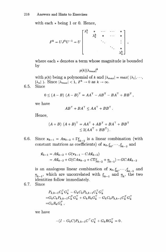
216 Answers and Hints to Exercises
with each * being 1 or o. Hence,
A~ * *A~ * *
F k = UJkU- 1 = U
where each * denotes a term whose magnitude is boundedby
p(k)IAmaxl k
with p(k) being a polynomial of k and IAmaxl = max( IAII,· .. ,IAnl ). Since IAmaxl < 1, F k ~ 0 as k ~ 00.
6.5. Since
we have
Hence,
(A+B) (A+B)T =AAT +ABT +BAT +BBT
:S 2(AAT + BBT).
6.6. Since Xk-l = AXk-2 + r~k_2 is a linear combination (withconstant matrices as coefficients) of xO'~o,··· '~k-2 and
Xk-l = AXk-2 + G(Vk-1 - CAXk-2)
= AXk-2 + G(CAXk-2 + cr~k_2 + '!lk-l) - GCAXk-2
is an analogous linear combination of Xo, ~o' ... '~k-2 and'!lk-l' which are uncorrelated with ~k-l and '!lk' the twoidentities follow immediately.
6.7. Since
Pk,k-I C-:Gl - GkCkPk,k-I C-:al=CkCkPk,k-IC"[cl + CkRkCl - CkCkPk,k-I C"[cl
=GkRkGl,
we have
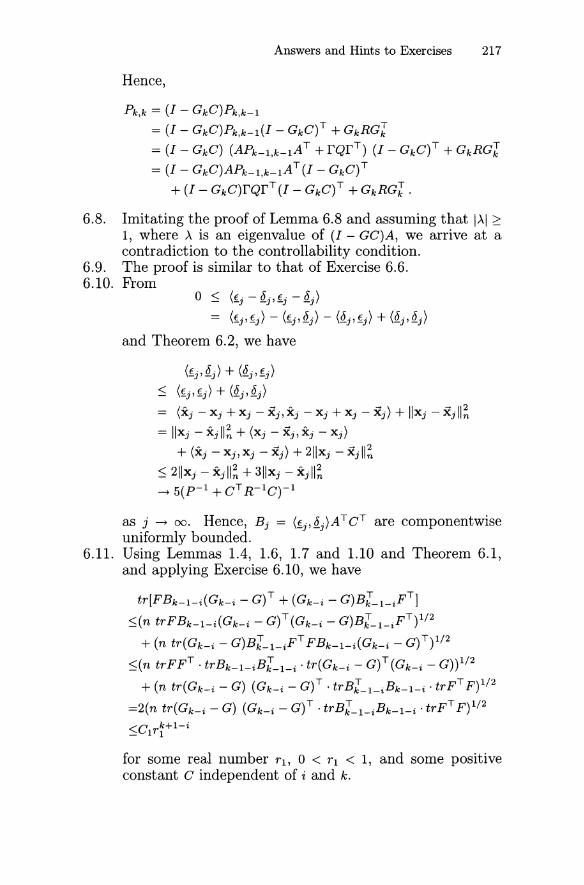
Answers and Hints to Exercises 217
Hence,
Pk,k = (1 - GkC)Pk,k-1
= (1 - GkC )Pk,k-I(1 - GkC )T + GkRGl
= (1 - GkC) (APk_l,k_IAT + rQrT) (1 - GkC)T + GkRGl
= (1 - GkC)APk_l,k_IAT (1 - GkC) T
+ (1 - GkC)rQrT (1 - GkC )T + GkRGl.
6.8. Imitating the proof of Lemma 6.8 and assuming that IAI ~1, where A is an eigenvalue of (1 - GC)A, we arrive at acontradiction to the controllability condition.
6.9. The proof is similar to that of Exercise 6.6.6.10. From
o < (E.-8. E.-8.)- -J -J'-J -J
= (fj' fj) - (fj' ~j) - (~j' fj) + (~j' ~j )
and Theorem 6.2, we have
(fj' ~j) + (~j' fj)
< (fj, fj) + (~j' ~j )
(Xj -Xj +Xj -Xj,Xj -Xj +Xj -Xj) + IIxj -Xjll~
- Ilx· - x·11 2 + (x· - x· x· - x·)- J J n J J' J J
+ (Xj - Xj,Xj - Xj) + 211xj - Xjll;
:S 211 x j - Xj 11; + 311 x j - Xj 11;-+ 5(P- 1 + CT R-IC)-I
as j -+ 00. Hence, Bj = (fj'~j)ATc T are componentwiseuniformly bounded.
6.11. Using Lemmas 1.4, 1.6, 1.7 and 1.10 and Theorem 6.1,and applying Exercise 6.10, we have
tr[PBk-I-i(Gk-i - G) T + (Gk-i - G)BJ_I_iPT ]
:S(n trPBk-I-i(Gk-i - G)T (Gk-i - G)BJ_I_iPT)I/2
+ (n tr(Gk-i - G)BJ_I_ipTPBk-I-i(Gk-i - G) T)I/2
:S(n trppT . trBk-I-iBJ_I_i· tr(Gk-i - G)T (Gk-i - G))1/2
+ (n tr(Gk-i - G) (Gk-i - G)T . trBJ_I_iBk-I-i . trpT p)I/2
=2(n tr(Gk- i - G) (Gk- i - G) T . trBJ_I_iBk-I-i . trFT F)I/2
<C r k +l - i- I I
for some real number rI, 0 < rl < 1, and some positiveconstant C independent of i and k.
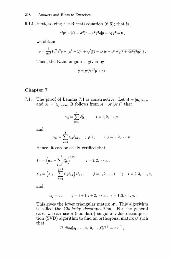
218 Answers and Hints to Exercises
6.12. First, solving the Riccati equation (6.6); that is,
c2p2 + [(1 - a2)r - c2,2q]p - rq,2 = 0,
we obtain
1p = 2c2 {c2
,),2q + (a2- l)r + V[(l - a2 )r - c2')'2q]2 + 4C2')'2 qr }.
Then, the Kalman gain is given by
9 = pcj(c2p + r) .
Chapter 7
7.1. The proof of Lemma 7.1 is constructive. Let A = [aij]nxnand AC = [Rij]nxn. It follows from A = AC(AC)T that
and
i
aii = LR;k,k=1
j
aij = L RikRjk , j =1= i ;k=1
i = 1,2,' .. , n,
i,j = 1,2,···,n.
Hence, it can be easily verified that
i-I 1/2
f ii = (aii - L f;k) , i = 1, 2, ... ,n,k=1j-l
fij = (aij - L fikfjk) / fj j , j = 1,2, ... ,i - 1; i = 2, 3, ... , n,k=1
and
j = i + 1, i + 2, ... , n; i = 1,2, ... , n.
This gives the lower triangular matrix AC. This algorithmis called the Cholesky decomposition. For the generalcase, we can use a (standard) singular value decomposition (8VD) algorithm to find an orthogonal matrix U suchthat
U diag[sl,···,Sr,o, ... ,O]UT =AAT ,
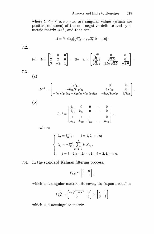
Answers and Hints to Exercises 219
where 1 :::; r :::; n, 81,'" ,8r are singular values (which arepositive numbers) of the non-negative definite and symmetric matrix AAT, and then set
A = U diag[JS1 ... VS; 0 ... 0], , r" , .
7.2.
L = [~0
n· [J20
o ](a) 2 (b) L = J2/2 m o .-2 J2/2 1.5/m J2]
7.3.(a)
[ l/f l1 0o ]L- 1 = -£21/£11£22 1/£22 o .
-£31/£11£33 + £32£21/£11£22£33 -£32/£22£33 1/£33
(b)
[bl1 0 0
)JL- 1 = b~lb22 0
bn1 bn2 bn3
where
i = 1,2,"" n;i
bij = -£711 L bik£kj,
k=j+1
j = i - 1, i - 2, ... ,1; i = 2,3, ... ,n.
7.4. In the standard Kalman filtering process,
which is a singular matrix. However, its "square-root" is
p1/2 _ [E/~ 0] [E 0]k,k - 0 1 ~ 0 1
which is a nonsingular matrix.
220 Answers and Hints to Exercises
7.5. Analogous to Exercise 7.1, let A == [aij]nxn and AU == [£ij]nxn.
It follows from A == AU(AU)T that
and
n
aii == L£;k'k=i
n
aij == L fikfjk ,
k=j
i == 1,2.···, n,
j =I i; i, j == 1,2,· .. ,n.
Hence, it can be easily verified that
i == 1,2,· .. , n,
n
f ij = (aij - L fikfjk )/fjj ,
k=j+l
j == i + 1, ... ,n; i == 1,2, ... ,n.
andj == 1,2, ... ,i - 1; i == 2,3, ... ,n.
This gives the upper-triangular matrix AU.7.6. The new formulation is the same as that studied in this
chapter except that every lower triangular matrix withsuperscript c must be replaced by the corresponding uppertriangular matrix with superscript u.
7.7. The new formulation is the same as that given in Section7.3 except that all lower triangular matrix with superscriptc must be replaced by the corresponding upper triangularmatrix with superscript u.
Chapter 8
8.1. (a) Since r 2 ==x2 +y2, we have
. x. y.r == -x + -y,
r r
so that r == v sinB and
r == iJ sinB + vB cosB.
Answers and Hints to Exercises 221
On the other hand, since tane = yjx, we have 8sec20 =(xy - xy)jx2 or
. xy - xy xy - xy vo= 2 20 = 2 = -cosO ,
x sec r r
so that.. . v2
r = a s~nO + -cos20r
and.. (iJr-vi') v·o= r 2 cosO - ;:OsinB
(ar - v2sinO) v2
= r 2 cosB - r 2sinOcosB .
(b)
[
V sinB ]x = f(x) := a sinO + vr
2cos2B .
(ar - v2sinO)cosfJ j r 2 - v2sinfJ cosO j r 2
(c)
xk[l] + hv sin(xk[3])
xk[2] + ha sin(xk[3]) + v2cos2(xk[3])jxk[1]
vcos (xk [3] ) j Xk [1]
(axk[l] - v2sin(xk[3]))cos(xk[3])jxk[l]2-v2sin(Xk [3])COS(Xk [3])/xk[1]2
andVk = [1 0 0 0 ]Xk + TJk ,
where Xk := [xk[l] xk[2] xk[3] xk[4]]T.(d) Use the formulas in (8.8).
8.2. The proof is straightforward.8.3. The proof is straightforward. It can be verified that
8.4. Taking the variances of both sides of the modified "observation equation"
Vo - Co(fJ)E(xo) = Co(O)xo - Co(B)E(xo) + '!lo'
222 Answers and Hints to Exercises
and using the estimate (vo - Co(B)E(xo))(vo - Co(B)E(xo))Tfor Var(vo - Co(B)E(xo)) on the left-hand side, we have
(vo - Co(B)E(xo))(vo - Co(B)E(xo))T
=Co(B)Var(xo)Co(B)T + Ro.
Hence, (8.13) follows immediately.8.5. Since
E(Vl) = Cl(B)Ao(B)E(xo) ,
taking the variances of both sides of the modified "observation equation"
VI - Cl (B)Ao(B)E(xo)
=Cl(B)(Ao(B)xo - Cl(B)Ao(B)E(xo) + r(B)~o) + '!1.l '
and using the estimate (VI -Cl(B)Ao(B)E(xo))(Vl -Cl(B)Ao(B)·E(xo))T for the variance Var(vl - Cl(B)Ao(B)E(xo)) on theleft-hand side, we have
(VI - Cl (B)Ao(fJ)E(xo))(Vl - Cl (B)Ao(B)E(xo)) T
=Cl(B)Ao(B)Var(xo)A~ (B)Ci (B) + Cl(B)ro(B)Qor~ (B)Ci (B) + RI·
Then (8.14) follows immediately.8.6. Use the formulas in (8.8) directly.8.7. Since fl. is a constant vector, we have Sk := Var(fl.) = 0, so
thatp, = V (x) = [var(xo) 0]
0,0 ar fl. 0 o·
It follows from simple algebra that
Pk,k-l = [~~] and Gk = [~]
where * indicates a constant block in the matrix. Hence,the last equation of (8.15) yields ~klk == ~k-llk-l·
8.8.
p, _ [po 0 ]0,0 - 0 So
Answers and Hints to Exercises 223
where ca is an estimate of Co given by (8.13); that is,
Chapter 9
{
Xk = -(a + /3 - 2)Xk-l - (1 - a)Xk-2 + aVk + (-a + (3)Vk-l
:h = -(a + (3 - 2)Xk-l - (1 - a)Xk-2 + kVk - kVk-l .
2(b) 0 < a < 1 and 0 < /3 < l~a.
9.2. System (9.11) follows from direct algebraic manipulation.9.3. (a)
(b)
[
I-a
<P = -/3lh-,lh2
-()
(1 - a)h (1 - a)h2 /21 - /3 h - /3h12
1 -,Ih 1 -,/2-()Ih -()h2 /2
-sa]-s/3/h-s,lh2
s(l - ())
det[zI - <1>] =z4 + [(a - 3) + /3 + ,/2 - (() - 1)s]z3
+ [(3 - 2a) - /3 +,/2 + (3 - a - /3 -,/2 - 3())s]z2
+ [(a - 1) - (3 - 2a - /3 + ,/2 - 3())s]z + (1 - a - ())s.
- zV(z-s) 2Xl = det[zI _ Ill] {az + h'/2 + (3 - 2a)z + (,/2 - j1 +an,X = zV(z - l)(z - s) {/3 - /3 }/h
2 det[zI _ <1>] z +, ,x = zV{z - 1)2(z - s) Ih2
3 det[zI _ <p] , ,
andw= zV(z-1)3 ().
det[zI - 4.>]
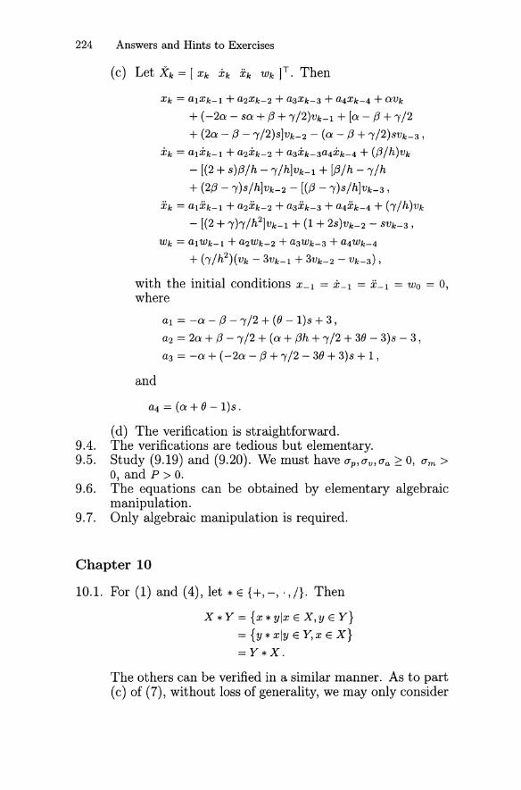
224 Answers and Hints to Exercises
Xk = alXk-1 + a2 Xk-2 + a3x k-3 + a4Xk-4 + aVk
+ (-2a - sa + ,8 + , /2)Vk-1 + [a - ,8 +,/2+ (2a - ,8 - , /2)S]Vk-2 - (a - ,8 +,/2)SVk-3 ,
Xk = alxk-l + a2x k-2 + a3x k-3a4x k-4 + (,8/h)Vk
- [(2 + s),8/h - ,/h]Vk-1 + [,8/h - ,/h
+ (2,8 - ,)S/h]Vk-2 - [(,8 - ,)S/h]Vk-3,
Xk = alxk-l + a2x k-2 + a3x k-3 + a4x k-4 + (,/h)Vk
- [(2 + ,),/h2]Vk_1 + (1 + 2S)Vk-2 - SVk-3,
Wk = alwk-l + a2Wk-2 + a3Wk-3 + a4Wk-4
+ (,/h2)(Vk - 3Vk-1 + 3Vk-2 - Vk-3),
with the initial conditions X-I = X-I = X-I = Wo = 0,where
al = -a - ,8 -,/2 + (0 - l)s + 3,
a2 = 2a + {3 - ,/2 + (a + ,8h + ,/2 + 38 - 3)s - 3 ,a3 = -a + (-2a - ,8 +,/2 - 38 + 3)s + 1 ,
and
a4 = (a + 8 - l)s.
(d) The verification is straightforward.9.4. The verifications are tedious but elementary.9.5. Study (9.19) and (9.20). We must have ap,av,aa 2: 0, am >
0, and p > o.9.6. The equations can be obtained by elementary algebraic
manipulation.9.7. Only algebraic manipulation is required.
Chapter 10
10.1. For (1) and (4), let * E {+,-, .,/}. Then
X * Y = {x * ylx E X,y E Y}
= {y * xly E Y,x E x}=y*x.
The others can be verified in a similar manner. As to part(c) of (7), without loss of generality, we may only consider
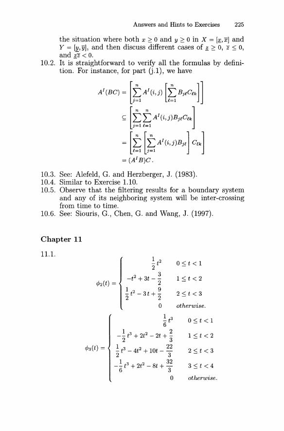
Answers and Hints to Exercises 225
the situation where both x 2 0 and y 2 0 in X = [;f, x] andy = [y, y], and then discuss different cases of ± 2 0, z :::; 0,and ±--Z < o.
10.2. It is straightforward to verify all the formulas by definition. For instance, for part (j.1), we have
A1(BC) = [~AI(i,j) [~BjlClk]]
~ [~~AI(i,j)BjlClk]
= [t [tA1(i,j)Bjl] Clk]l=l J=l
= (A1B)C.
10.3. See: Alefeld, G. and Herzberger, J. (1983).10.4. Similar to Exercise 1.10.10.5. Observe that the filtering results for a boundary system
and any of its neighboring system will be inter-crossingfrom time to time.
10.6. See: Siouris, G., Chen, G. and Wang, J. (1997).
Chapter 11
11.1.1 2-t2
2 3-t + 3t --2
1 2 9-t -3t+2 2
o1 3-t6
1 3 2 2- - t + 2t - 2t + -2 3
1 3 2 22- t - 4t + lOt - -2 3
1 3 2 32- - t + 2t - 8t + -6 3
o
O:::;t<l
1:::;t<2
2:::;t<3
otherwise.
O:::;t<l
1::;t<2
2:::;t<3
3:::;t<4
otherwise.
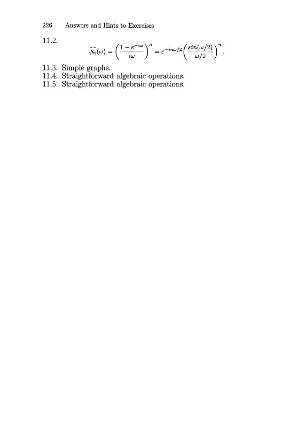
226 Answers and Hints to Exercises
11.2.;j;;,(w) = C-i:-iW)n= e-inw/2 (si~1f2))n.
11.3. Simple graphs.11.4. Straightforward algebraic operations.11.5. Straightforward algebraic operations.
Subject Index
adaptive Kalman filtering 182
noise-adaptive filter 183
adaptive system
identification 113,115
affine model 49
a - {3 tracker 140
a - {3 - , tracker 136
a - {3 - , - () tracker 141,180
algorithm for real-time
application 105
angular displacement 111,129
ARMA (autoregressive
moving-average) process 31
ARMAX (autoregressive
moving-average model
with exogeneous inputs) 66
attracting point 111
augmented matrix 189
augmented system 76
azimuthal angular error 47
Bayes formula 12
Cholesky factorization 103
colored noise (sequence
or process) 67,76,141
conditional probability 12
controllability matrix 85
controllable linear system 85
correlated system and
measurement noise processes 49
covariance 13
Cramer's rule 132
decoupling formulas 131
decoupling of filtering
equation 131
Descartes rule of signs 140
determinant preliminaries 1
deterministic input sequence 20
digital filtering process 23
digital prediction process 23
digital smoothing estimate 178
digital smoothing process 23
elevational angular error 47
estimate 16
least-squares optimal
estimate 17
linear estimate 17
minimum trace variance
estimate 52
minimum variance
estimate 17,37,50
optimal estimate 17
optimal estimate
operator 53
unbiased estimate 17,50
event 8
simple event 8
expectation 9
conditional expectation 14
228 Subject Index
extended Kalman filter 108,110,115
FIR system 184
Gaussian white noise sequence 15,117
geometric convergence 88
IIR system 185
independent random variables 14
innovations sequence 35
inverse z-transform 133
Jordan canonical form 5,7
joint probability
distribution (function) 10
Kalman filter 20,23,33
extended Kalman filter 108,110,115
interval Kalman filter 154
limiting Kalman filter 77,78
modified extended Kalman filter 118
steady-state Kalman filter 77,136
wavelet Kalman filter 164
Kalman-Bucy filter 185
Kalman filtering equation
(algorithm, or process)
23,27,28,38,42,57,64,72-74,76,108
Kalman gain matrix 23
Kalman smoother 178
least-squares preliminaries 15
limiting (or steady-state)
Kalman filter 78
limiting Kalman gain matrix 78
linear deterministic/ stochastic
system 20,42,63,143,185
linear regulator problem 186
linear state-space (stochastic) system
21,33,67,78,182,187
LU decomposition 188
marginal probability
density function 10
matrix inversion lemma 3
matrix Riccati equation 79,94,132,134
matrix Schwarz inequality 2,17
minimum variance estimate 17,37,50
modified extended Kalman filter 118
moment 10
nonlinear model (system) 108
non-negative definite matrix 1
normal distribution 9
normal white noise sequence 15
observability matrix 79
observable linear system 79
optimal estimate 17
asymptotically optimal estimate 90
optimal estimate operator 53
least-squares optimal estimate 17
optimal prediction 23,184
optimal weight matrix 16
optimality criterion 21
outcome 8
parallel processing 189
parameter identification 115
adaptive parameter
identification algorithm 116
positive definite matrix 1
positive suqare-root matrix 16
prediction-correction 23,25,31,39,78
probablity preliminaries 8
probablity density function 8
conditional probability
density function 12
joint probability
density function 11
Gaussian (or normal) probability
density function -9,11
probability distribution 8,10
function 8
joint probability
distribution (function) 10
radar tracking model
(or system) 46,47,61,181
random sequence 15
randon signal 170
random variable 8
independent random variables 13
uncorrelated random variables 13
random vector 10
range 47,111
real-time application 61,73,93,105
real-time estimation/decomposition 170
real-time tracking 42,73,93,134,139
sample space 8
satellite orbit estimation 111
Schur complement technique 189
Schwarz inequality 2
matrix Schwarz inequality 2,17
vector Schwarz inequality 2
separation principle 187
sequential algorithm 97
Subject Index 229
square-root algorithm 97,103
square-root matrix 16,103
steady-state (or limiting)
Kalman filter 78
stochastic optimal control 186
suboptimal filter 136
systolic array 188
implementation 188
Taylor approximation 47,122
trace 5
uncorrelated random variables 13
variance 10
conditional variance 14
wavelets 164
weight matrix 15
optimal weight matrix 16
white noise sequence (process)
15,21,130
Gaussian (or normal) white
noise sequence 15,130
zero-mean Gaussian white
noise sequence 21
Wiener filter 184
z-transform 132
inverse z-transform 133