Katsushi Imai Md. Shafiul Azam - University of Manchesterhummedia.manchester.ac.uk/schools/soss/economics/discussionpaper… · 1 Does Microfinance Reduce Poverty in Bangladesh? New

Economics Discussion Paper Series EDP-1019

Does Microfinance Reduce Poverty in Bangladesh? New Evidence from

Household Panel Data

Katsushi Imai

Md. Shafiul Azam

October 2010

Economics School of Social Sciences

The University of Manchester Manchester M13 9PL

1

Does Microfinance Reduce Poverty in Bangladesh? New Evidence from Household Panel Data*

Katsushi S. Imai

Economics, School of Social Sciences, University of Manchester, UK & Research Institute for Economics & Business Administration (RIEB), Kobe University, Japan

& Md. Shafiul Azam

Economics, School of Social Sciences, University of Manchester, UK

30th September 2010

Abstract

The purpose of the present study is to examine whether microfinance reduces poverty in Bangladesh drawing upon the nationally representative household panel data covering 4 rounds from 1997 to 2005. A special attention was drawn to the issue of endogeneity by applying treatment effects model and propensity score matching (PSM) for the participants and non-participants of microfinance programmes. It has been confirmed by treatment effects model applied to panel data that household access to loans for productive purposes from microfinance institutions (MFIs) significantly increased per capita household income, while simple household access to general loans from MFIs did not. This suggests that purpose and monitoring of how clients use the loans is important for increasing household income, and thus decreasing household poverty. However, the application of treatment effects model and PSM to each cross-sectional component of the panel data shows that the poverty reducing effect of MFI on poverty was significantly reduced over the years. This suggests the need of more attention to be drawn to the primary purpose of microcredit, that is, poverty reduction, and also to monitoring loan usages in the situations where the profits of MFIs became increasingly squeezed and their activities became more commercialised under severe competitions among MFIs in recent years.

Key words: microfinance, MFI (microfinance institution), microcredit, poverty, Bangladesh

JEL codes: C30, C31, G21, I32

*Corresponding Author: Katsushi Imai (Dr) Department of Economics, School of Social Sciences University of Manchester, Arthur Lewis Building, Oxford Road, Manchester M13 9PL, UK Phone: +44-(0)161-275-4827 Fax: +44-(0)161-275-4928 E-mail: [email protected]

Acknowledgement This study is funded by IFAD (International Fund for Agricultural Development). The authors are grateful to Raghav Gaiha and Ganesh Thapa for their support and guidance throughout this study. The first author wishes to thank RIEB, Kobe University for generous research support during his stay in 2010 and acknowledge valuable comments and advice from Shoji Nishijima, Takahiro Sato and seminar participants at Kobe University. The paper has greatly benefited from comments from Thankom Arun and Samuel Annim. The views expressed are our personal views and not necessarily of the organisations to which we are affiliated.

2

Does Microfinance Reduce Poverty in Bangladesh? New Evidence from Household Panel Data*

I. Introduction

The idea that microfinance helps poor people build businesses, increase their income and exit

poverty has turned into a global movement, so called ‘microfinance revolution’, to fight

against poverty over the last three decades. This is reflected in the significant increase of

donor countries’ investment in microfinance sector in recent years. The poor tend to have

limited access to services from formal financial institutions in less developed countries due

to, for example, (i) the lack of physical collateral of the poor; (ii) the cumbersome procedure

to start transaction with formal banks, which would discourage those without education from

approaching the banks; and (iii) lack of supply of credit in the rural areas related to urban

biased banking networks and credit allocations. The hallmark of microfinance revolution is

the system of group lending based on the joint liability or ‘social capital’ of communities

which would guarantee to repay loans. Here the poor with no physical collateral are allowed

to form a group to gain access to credit and the repayment rate is kept high because of, for

example, mutual monitoring, sanction against non-repayment of the member or incentives to

retain the individual reputation or credit within a community (e.g. Armendáriz and Morduch,

2005, Besley and Coate, 1995, Ahlin and Townsend, 2007). 1

The last thirty years witnessed a phenomenal growth in microfinance sector serving about

40 million clients with an outstanding loan portfolio of US$17 billion in mid-2006 and the

projected market size could be around US$250-300 billion in near future (Ehrbeck, 2006).

However, the argument that microfinance responds to the derived demand for borrowing to

support self-employment and small business has come under intense scrutiny in recent years.

Even the hard core of pro-microfinance researchers now broadly agree that attention should

be drawn to both supply and demand sides of microfinance in order for the sector to have a

3

noticeable poverty reducing effects. As Robert Pollin (2007, p.2) notes, micro-enterprises

“need a vibrant, well functioning domestic market itself that encompasses enough people

with enough money to buy what these enterprises have to sell”. Moreover, as noted by

Bateman and Chang (2009), microfinance neglects the crucial role of scale economies and it

produces an oversupply of inefficient micro-enterprises that could undermine the

development of more efficient small and medium industries (SMEs) that would be potentially

able to reduce unit costs and register productivity growth in the long run. However, shifting

the donor’s fund away from very small groups or enterprises (target of microfinance

institutions) to SMEs could imply the neglect of the very poor who are credit constrained and

could increase poverty in the country given the recent evidence that has shown a negative and

statistically significant association between the MFI loans and poverty based on cross-

country data (Imai et al. 2010). The development agencies of donor countries or government

will have to make sure whether the benefits to programme participants are sustainable and

large enough to make a dent in the poverty of participants and society at large.

Bangladesh has recorded a modest 4-6 % growth within a stable macroeconomic

framework in recent years. The poverty trend has shown a consistent decline in poverty

incidence over the years, especially in rural areas. However, aggregate poverty rates still

remain dauntingly high. According to the estimates based on the Household Income and

Expenditure Surveys (HIES) of the Bangladesh Bureau of Statistics, poverty head count ratio

declined from 58.8 % in 1991 to 48.9 % per cent in 2000 and it further declined to 40.0 % in

2005. So poverty has declined on average just above one percentage point a year since the

1990s. The observed improvement holds true for the distributionally sensitive poverty

measures: the poverty gap ratio reduced from 17.2 % to 12.9 % and the squared poverty gap

ratio from 6.8 % to 4.6 % during the same period from 2000 to 2005. This indicates that the

situation of the poorest also improved during this period, though there existed the very poor

4

as well as inequality among the poor even in 2005. The head count ratio in rural area reduced

from 52.3 % in 2000 to 43.8 % in 2005. However, the absolute number of people living

below poverty line was in fact on the rise –a staggering 56 million people were found to be

poor in 2005. The corresponding figure was 55 million in 2000. Similarly, hard core poverty

remains almost same during the period 2000-2005 (18.8 % and 18.7 % in 2000 and 2005

respectively). So poverty reduction remains the most daunting challenge for Bangladesh.

Bangladesh, the birthplace of microfinance, is credited with the largest and most vibrant

microcredit sector in the world. Microcredit programmes are implemented in Bangladesh by

host of formal financial institutions, specialized government organizations and semi-formal

financial institutions (nearly 1000 NGOs-MFIs). Furthermore, with a view to coordinating

the flow of funds to appropriate use and NGOs-MFI activities, the Palli Karma Sahayak

Foundation (the Bengali acronym PKSF and can be translated into English as “Rural

Employment Support Foundation”) came into being in 1990. The growth in the MFI sector,

in terms of the number of MFIs as well as total membership, was phenomenal during the

1990s and after 2000. The effective coverage would be around 17.32 million borrowers. The

total amount is 24.25 million due to overlapping –one borrower taking loan form more than

one MFI and the extent of overlapping may be as high as 40% (PKSF, 2006). Out of 17.32

million borrowers covered by micro credit programmes, about 62% were below the poverty

line, that is, 10.74 million poor borrowers were covered by MFI programmes. 56 million

people were estimated to be poor in 2005. 53% of those or 29.26 million were supposed to be

economically active and were potentially the target group of microfinance operation.

Therefore, there was still scope for further extending the coverage of microcredit

programmes in 2005 to an approximate 18.52 million borrowers who were poor and

economically active but not covered by MFI programmes (Ahmed, 2007).

5

The main purpose of the present study tests whether microfinance reduces poverty in

Bangladesh drawing upon the nationally representative household panel data covering 4

rounds, 1997-98, 1998-99, 1999-2000, and 2004-05. A special attention is drawn to the issue

of endogeneity on participation in microfinance by applying treatment effects model and

propensity score matching for the participants and non-participants of microfinance

programmes.

The rest of the paper is organized as follows. The next section surveys the literature on

poverty and microfinance in Bangladesh. Section III describes briefly the survey design and

data. Section IV explains the underlying econometric intuition of treatment effect model and

Section V summarizes the econometric results and findings. The final section offers

concluding observations.

II. The Literature Review on Poverty and Microfinance

Despite the data limitations and methodological problems, e.g. on dealing with the sample

selection bias associated with microfinance participation, there are a few rigorous studies to

assess the impact of microfinance on poverty. The findings of a set of studies summarised by

Hulme and Mosley (1996) are somewhat provocative: households with initial higher income

above the poverty line benefited from microfinance and enjoyed sizeable positive impacts,

while poorer households below the poverty line did not. A majority of those with their initial

income below the poverty line actually ended up with less incremental income after obtaining

microcredit, as compared to a control group which did not get any loans from MFI. Pitt and

Khandker (1998) carried out a survey in 1991/92 involving about 1800 households in

Bangladesh and found that for every 100 taka borrowed by a woman, household consumption

expenditure increased by 18 taka. For a male borrower, the figure is 11 taka. They estimated

the poverty reducing effect of three major microfinance institutions in Bangladesh namely –

6

Bangladesh Rural Advancement Committee (BRAC), Grameen Bank, and Bangladesh Rural

Development Board (BRDB). Moderate and ultra poverty was reduced by about 15 % and 25

% for households who were BRAC members for up to three years. Similar results are found

for Grameen Bank and BRDB members.

Drawing upon the follow up survey in 1998/99, Khandker (2005) found resounding results

at both micro and aggregate levels: microcredit continued to contribute to reducing poverty

among poor borrowers and within local economy. The impact appears to be greater for

households who were initially the extremely poor (18 percentage point drop in extreme

poverty in seven years) compared to moderate poor households (8.5 percentage point drop).

These results differ from earlier evidence that pointed to moderate poor borrowers having

benefited more than extremely poor borrowers who tended to have a number of constraints

(e.g. fewer income sources, worse health and education) which prevent them from investing

the loan in a high-return activity (Wood and Sharif 1997). The finding that better off

households benefiting more was also borne out by detailed case-study evidence (Farashuddin,

and Amin,1998) and by comparing participants of credit programmes who cater to different

socio-economic groups (Montgomery et al., 1996).

The general conclusions of Pitt and Khandker (1998) and Khandker (2005) about the

impact of microcredit on poverty include: (i) microcredit was effective in reducing poverty

generally, (ii) this is especially true when borrowers were women, and (iii) the extremely

poor benefit most in 1998/99. However, the last point has been contested and questioned by

Morduch (1998) and Roodman and Morduch (2009). Morduch (1998) using the same data set

but a different way of correcting sample selection bias, finds that microcredit had a

consumption smoothing effect for households who were at risk, that is, microcredit helped

families smooth their consumption expenditures and lessen the pinch of hunger in lean

periods. But the study broadly failed to find any significant impact on household

7

consumption levels and on income poverty. A recent study by Roodman and Morduch (2009)

found similar results and pointed to the methodological flaws and econometric issues on the

absence of robust and decisive statistical evidence in these literatures. Consumption data

from 1072 households in one district of Bangladesh were used to show that the largest effect

on poverty occurs when a moderate-poor BRAC client borrows more than tk10,000

(US$200) in cumulative loans (Zaman, 1998). In other words, there may be a threshold level

of credit above which a household gains most in terms of increases in income.

The relationship between poverty and microfinance is unclear outside Bangladesh. Two

recent studies that attempted to overcome the sample selection problem by using randomized

sample selection methods also came up with not so resounding evidence in favour of

microcredit. Banerjee, Duflo, Glennerster and Kinnan (2009) did not find much strong

average impact; i.e., the impact on measures of health, education, or women’s decision-

making among the slum dwellers in the city of Hyderabad, India was negligible. The study

by Karlan and Zinman (2009) took a similar method to the Philippines, with a focus on the

traditional microcredit for small business investment. Profits rise, but largely for men and

particularly for men with higher incomes. Moreover, the increases in profits appear to arise

from business contractions that yielded smaller, lower-cost (and more profitable) enterprises.

Imai et al. (2010), however, found that the loans from MFI for productive purposes reduced

significantly multifaceted household poverty, which was defined in terms of assets,

employment, health facilities, and food security, using the survey data in India in 2000.

Given the inconclusive and ambiguous nature of evaluation outcomes and increasing

involvement of MFIs both in terms of number of institutions and resources in poverty

reduction efforts, it is important to have a deeper look into the relationship between

microfinance or microcredit and poverty. The present study aims to provide new evidence on

the impact of microfinance on poverty in rural Bangladesh using a large and nationally

8

representative panel data. The indicator for wellbeing/poverty is per capita household

income. This paper seeks to answer the question –whether access to loans from MFIs for

general purposes (or loans from MFIs for productive purposes) reduced poverty in rural

Bangladesh. Ideally, the impact of microfinance should be ascertained by a counterfactual

approach- what would have happened to a person who took a loan from a MFI if she or he

had not done so. However, such a counterfactual is never observed in reality. The easiest and

intuitive method is to compare the welfare or income of borrowers and non-borrowers. But

such comparison is problematic for a number of reasons. First, MFIs are not distributed

across regions randomly due to endogenous programme placement where MFIs generally

target poorer households, or the constituent of core group of clientele for the services of MFIs

are poorer households. Second, there is a self selection problem, that is, whether an

individual participates in the MFI programme is determined by herself, not by chance. That

is, within the area where the MFI programme is available, individuals sharing similar socio-

cultural backgrounds (e.g., education, age or religion) might have different levels of

entrepreneurial skills and latent ability leading to different probabilities to their participating

in certain programme. Hence, it is essential to take into account the endogeneity or self-

selection problems in assessing the impact of microfinance.

III. Design of Survey and Data

(a) Details of Survey

The four-round panel survey was carried out by the Bangladesh Institute of Development

Studies (BIDS) for Bangladesh Rural Employment Support Foundation (PKSF) with funding

from the World Bank. All four rounds of the survey were conducted during the December-

February period in 1997-98, 1998-99, 1999-2000, and 2004-05. The survey covered a sample

of 13 PKSF’s Partner Organization (PO) and over 3000 households in each round distributed

9

evenly throughout Bangladesh so as to obtain a nationally representative data set for the

evaluation of microfinance programmes in the country (different districts spanning 91

villages from around 23 thanas).

A sample of villages under each of the selected MFI was drawn through stratified

random sampling. The stratification was based on the presence or absence of microfinance

activities. The non-programme or control villages were selected from the neighbouring

villages. At each PO, six to eight villages were selected depending on the availability of

control villages. In selecting survey households, the universe of households in the programme

villages drawn from the census was grouped according to their eligibility status. A household

is said to be eligible if it owns 50 decimals (half an acre) or less of cultivable land.

Participation status of the household is defined using the net borrowing from a MFI. If a

household is not a participant in a given round, the net borrowing is zero for that household.

From the village census list, 34 households were drawn from each of the programme and

non-programme villages. The proportion of eligible and non-eligible households was kept at

around 12:5 and the sample size within the programme and control villages was determined

accordingly. The ratio is chosen to reflect the average participants to non-participants ratio of

the population in the village. This is the largest and the most comprehensive data of its kind

so far in Bangladesh collected with detailed information on a number of socio economic

variables, including household demographics, consumption, assets and income, health and

education and participation in microcredit programmes.

(b) Descriptive Statistics and Definition of Variables

The study uses two different definitions of access to Microfinance Institutions: first, whether

a household is a client of any MFI and takes loans for general purposes or not, and second,

whether a household has actually taken a loan from any MFI for productive purpose or not.

The first definition is used to observe the effect of taking general loans from MFI on per

10

capita household income and thus on poverty. The second is concerned with whether the

household has taken loans for productive activities (and has an outstanding balance of loans

at the time of survey) leading to an increase in production, for example, starting a small

business or other self employment activities, like small scale poultry or cattle rearing. Loans

used for consumption or other non-productive activities like marriage or dowry are excluded

from this category.

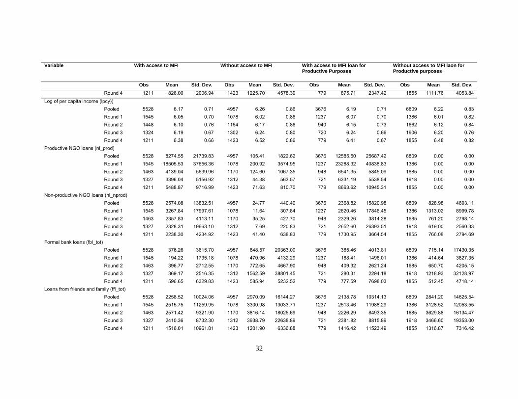
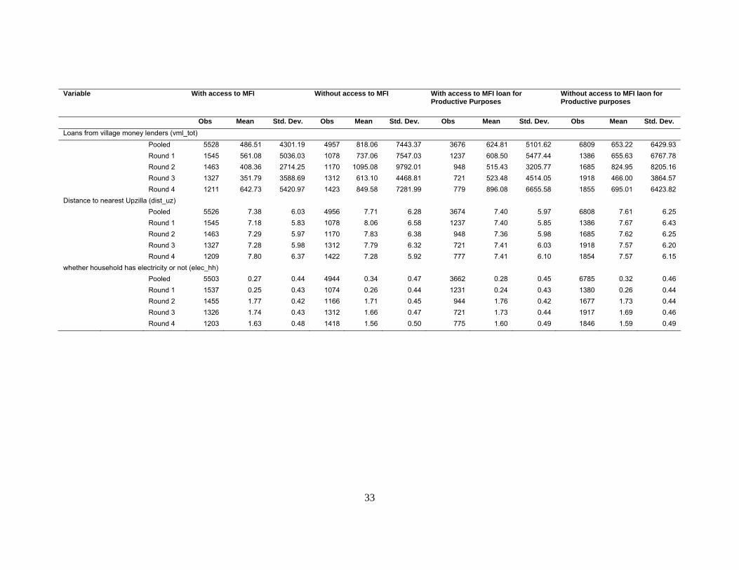
Appendix provides the descriptive statistics of the variables for the sample households

with access to loans from MFI and for those without. As shown by the number of

observations, more than a half of the sample household have access to MFI loans. About a

half of them have access to loans from MFI for productive purposes. In general, there is a

relatively negligible difference between the descriptive statistics of each variable for the

households with and without access to loans from MFIs (or with access to loans from MFIs

for productive purposes) and for those without.

The average household size is about 6 for both categories of households. Head of the

households are categorised into four groups depending on their educational level – illiterate,

completing primary education, secondary education, or higher education. Similarly,

occupation of the head of the households is grouped into six distinct categories – farmers,

agricultural wage labourers, non-agricultural wage labourers, small business, professionals

(which comprises of teachers, lawyers, doctors and other salaried employees), and others

(beggars, students, retired persons, disabled, unemployed etc.). However, per capita income

is generally higher for those who do not take MFI loan or participate in MFI programmes.

This does not necessarily imply that taking loans from MFIs reduces per capita income due to

the aforementioned sample selection bias. About 93 per cent of the households are male

headed, mainly due to the sample design where households in a village are selected randomly

even though a majority of the MFI clients are female.

11

IV. Methodology

(a) Treatment Effects Model

To address the self-selection problem, the present study applies the treatment effects model, a

version of the Heckman sample selection model (Heckman, 1979). The treatment effect

model estimates the probit model in the first stage and in the second stage, per capita income,

our indicator for poverty, is estimated by OLS while sample selection is corrected by using

the estimates of the probability of participation in the microfinance programme in the first

stage. The model is fitted by a full maximum likelihood (Maddala 1983). The merits of the

treatment effects model include – (i) the degree of sample selection bias is explicitly taken

into account and (ii) the determinants of the dependent variables in the second stage are fully

identified. However, the treatment effects model imposes strong distributional assumptions

for the functions in both stages and the final results are highly sensitive to the choice of

explanatory variables and the instrument.

In the first stage, access to loans from MFIs is estimated by the probit model where a

dependent variable is whether a household had a member who took loans from a MFI for

general purposes (or for productive purposes). In the second, the model estimates log of per

capita income after controlling for the inverse Mills ratio which reflects the degree of sample

selection bias. Distance from nearest ‘Upzilla’, the business and administrative hub where

most of the local services including marketing and financial are available, is used as an

instrument. This satisfies the exclusion condition as it correlated with participation in a

microfinance programme, but not with income of the households. People living nearby

should have better business opportunities leading to higher demand for credit than those

living far away. But this does not directly affect per capita income.

The merit of treatment effects model is that sample selection bias is explicitly

estimated by using the results of probit model. However, the weak aspects include (i) strong

12

assumptions are imposed on distributions of the error terms in the first and the second stages,

(ii) the results are sensitive to choice of the explanatory variables and instruments, and (iii)

valid instruments are rarely found in the non-experimental data.

The selection mechanism by the probit model above can be more explicitly specified

as (e.g., Greene, 2003):

ii*i uXD (1)

and 0uXDif1D ii*i

*i

otherwise0D*i

where )X(X1DPr iii

)X(1X0DPr iii

*iD is a latent variable. In our case, iD takes 1 if a household has access to and 0 otherwise

and iX is a vector of household characteristics and other determinants. denotes the

standard normal cumulative distribution function.

The linear outcome regression model in the second stage is specified below to examine

the determinants of poverty, denoted as iW . That is,

iiii DZW (2)

iiu ~ bivariate normal ,,1,0,0 .

where is the average net wealth benefit of accessing loans from MFIs.

Using a formula for the joint density of bivariate normally distributed variables, the

expected poverty for those with access to MFI loans is written as:

i

ii

iiiii

X

XZ

1DEZ1DWE

(3)

where is the standard normal density function. The ratio of and is called the inverse

Mills ratio.

13

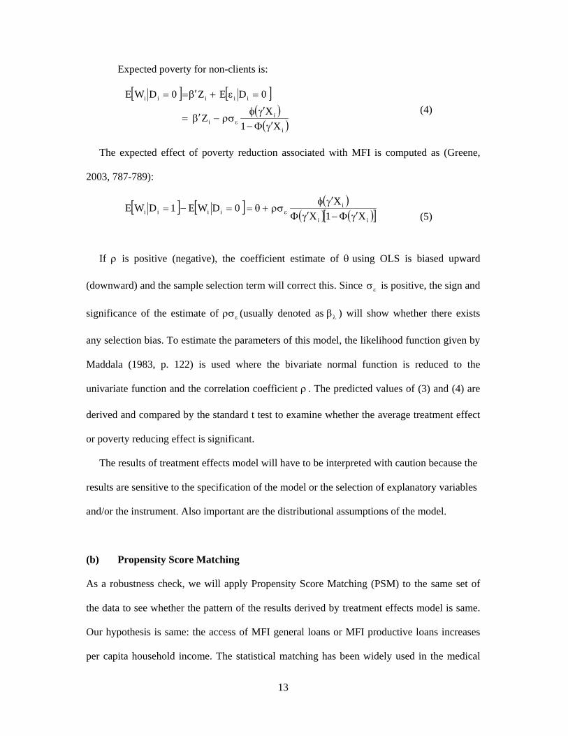
Expected poverty for non-clients is:

i

ii

iiiii

X1

XZ

0DEZ0DWE

(4)

The expected effect of poverty reduction associated with MFI is computed as (Greene,

2003, 787-789):

ii

iiiii X1X

X0DWE1DWE

(5)

If is positive (negative), the coefficient estimate of using OLS is biased upward

(downward) and the sample selection term will correct this. Since is positive, the sign and

significance of the estimate of (usually denoted as ) will show whether there exists

any selection bias. To estimate the parameters of this model, the likelihood function given by

Maddala (1983, p. 122) is used where the bivariate normal function is reduced to the

univariate function and the correlation coefficient . The predicted values of (3) and (4) are

derived and compared by the standard t test to examine whether the average treatment effect

or poverty reducing effect is significant.

The results of treatment effects model will have to be interpreted with caution because the

results are sensitive to the specification of the model or the selection of explanatory variables

and/or the instrument. Also important are the distributional assumptions of the model.

(b) Propensity Score Matching

As a robustness check, we will apply Propensity Score Matching (PSM) to the same set of

the data to see whether the pattern of the results derived by treatment effects model is same.

Our hypothesis is same: the access of MFI general loans or MFI productive loans increases

per capita household income. The statistical matching has been widely used in the medical

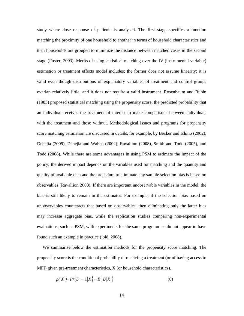
14

study where dose response of patients is analysed. The first stage specifies a function

matching the proximity of one household to another in terms of household characteristics and

then households are grouped to minimize the distance between matched cases in the second

stage (Foster, 2003). Merits of using statistical matching over the IV (instrumental variable)

estimation or treatment effects model includes; the former does not assume linearity; it is

valid even though distributions of explanatory variables of treatment and control groups

overlap relatively little, and it does not require a valid instrument. Rosenbaum and Rubin

(1983) proposed statistical matching using the propensity score, the predicted probability that

an individual receives the treatment of interest to make comparisons between individuals

with the treatment and those without. Methodological issues and programs for propensity

score matching estimation are discussed in details, for example, by Becker and Ichino (2002),

Dehejia (2005), Dehejia and Wahba (2002), Ravallion (2008), Smith and Todd (2005), and

Todd (2008). While there are some advantages in using PSM to estimate the impact of the

policy, the derived impact depends on the variables used for matching and the quantity and

quality of available data and the procedure to eliminate any sample selection bias is based on

observables (Ravallion 2008). If there are important unobservable variables in the model, the

bias is still likely to remain in the estimates. For example, if the selection bias based on

unobservables counteracts that based on observables, then eliminating only the latter bias

may increase aggregate bias, while the replication studies comparing non-experimental

evaluations, such as PSM, with experiments for the same programmes do not appear to have

found such an example in practice (ibid. 2008).

We summarise below the estimation methods for the propensity score matching. The

propensity score is the conditional probability of receiving a treatment (or of having access to

MFI) given pre-treatment characteristics, X (or household characteristics).

XDEXDPr)X(p 1 (6)

15

where 1,0D is the binary variable on whether a household had access to MFIs (1) or not

(0) and X is a multidimensional vector of pre-treatment characteristics or time-invariant or

relatively stable household characteristics in our context. It was shown by Rosenbaun and

Rubin (1983) that if the exposure to MFI is random within cells defined by X, it is also

random within cells defined by p(X) or the propensity score.

The policy effect of MFI can be estimated in the same way as in Becker and Ichino

(2002) as:

101

1

1

01

01

01

iiiiiii

iiii

ii

D)X(p,DWE)X(p,DWEE

)X(p,DWWEE

DWWEi

(7)

where i denotes the i-th household, i1W is the potential outcome (per capita household

income) in the two counterfactual situations with access to MFI and without. So the first line

of the equation states that the policy effect is defined as the expectation of the difference of

per capita household income of the i-th household with access to MFI and that for the same

household in the counterfactual situation where it would not have had access to MFI. The

second line is same as the first line except that the expected policy effect is defined over the

distribution of the propensity score. The last line is the policy effect as an expected difference

of the expected per capita household income score for the i-th household with access to MFI

given the distribution of the probability of accessing MFI and that for the same household

without MFI given the same distribution.

Under certain conditions2, the policy effect can be estimated by the procedures described

in Becker and Ichino (2002) and Smith and Todd (2005). Each procedure involves estimating

probit or logit model:

))X(h(X1DPr iii (8)

16

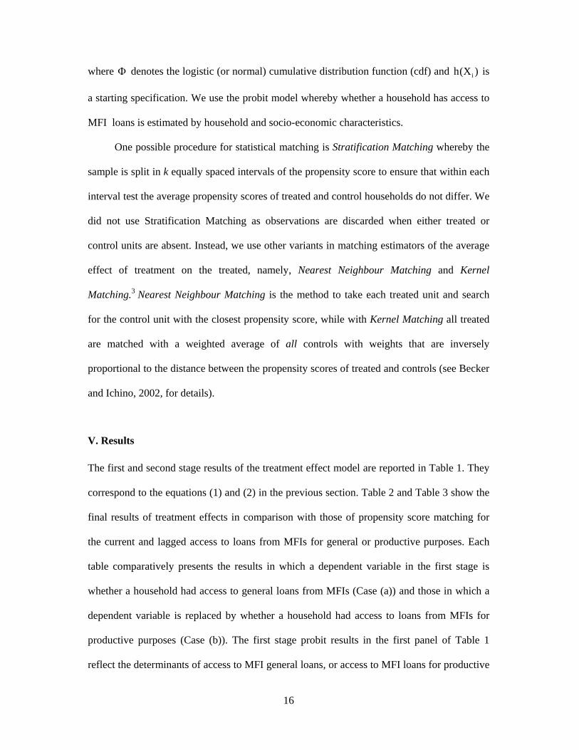
where denotes the logistic (or normal) cumulative distribution function (cdf) and )X(h i is

a starting specification. We use the probit model whereby whether a household has access to

MFI loans is estimated by household and socio-economic characteristics.

One possible procedure for statistical matching is Stratification Matching whereby the

sample is split in k equally spaced intervals of the propensity score to ensure that within each

interval test the average propensity scores of treated and control households do not differ. We

did not use Stratification Matching as observations are discarded when either treated or

control units are absent. Instead, we use other variants in matching estimators of the average

effect of treatment on the treated, namely, Nearest Neighbour Matching and Kernel

Matching.3 Nearest Neighbour Matching is the method to take each treated unit and search

for the control unit with the closest propensity score, while with Kernel Matching all treated

are matched with a weighted average of all controls with weights that are inversely

proportional to the distance between the propensity scores of treated and controls (see Becker

and Ichino, 2002, for details).

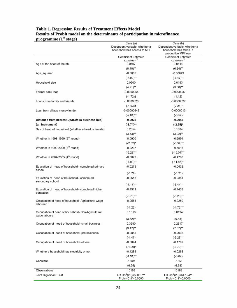
V. Results

The first and second stage results of the treatment effect model are reported in Table 1. They

correspond to the equations (1) and (2) in the previous section. Table 2 and Table 3 show the

final results of treatment effects in comparison with those of propensity score matching for

the current and lagged access to loans from MFIs for general or productive purposes. Each

table comparatively presents the results in which a dependent variable in the first stage is

whether a household had access to general loans from MFIs (Case (a)) and those in which a

dependent variable is replaced by whether a household had access to loans from MFIs for

productive purposes (Case (b)). The first stage probit results in the first panel of Table 1

reflect the determinants of access to MFI general loans, or access to MFI loans for productive

17

purposes. The second panel of Table 1 presents the results of treatment effects model. The

final result in Table 3, the first row (denoted as ‘panel data’) of Case (a) and that of Case (b)

show that the loans from MFI for productive purposes increased per capita household income

significantly, but general MFI loans did not. This suggests the importance of loan purpose

and monitoring.

(Table 1 to be inserted around here)

As shown by Case (a) of the first panel of Table 1, the coefficient estimate of age of the

head of the household is positive and significant, which implies that a household with older

head is more likely to have a member taking a general loan from MFIs, but the statistically

significant and negative coefficient estimate of ‘age squared’ suggests a non-linear effect of

age of the head. The positive and significant coefficient estimate of household size implies

that larger households have higher probability of having members who participated in

microfinance programmes. In the participation equation, the coefficient estimate of sex of the

head of the household, whether a head is female or not, is positive and significant. Given that

microfinance targets women, the result implies that a household headed by a woman is more

likely to have a participant in the MFI programmes than a male headed household. The

coefficient estimates of all the non-MFI sources of borrowing are negative and significant,

which reflects the fact that those who do not have access to, or are excluded from the

traditional sources of credit tend to get loans from MFI.4 The coefficient of distance from the

nearest Upzilla (a business hub), an instrument for the treatment effects model, is negative

and significant. This indicates that a household living closer to the nearest town with Upzilla

are more likely to participate in a microcredit programme than those who live far away. This

makes sense because Upzilla provides banking, marketing and other essential services for

micro businesses and enterprises to market their products.

18

The coefficient estimates of the education dummies are all negative and significant except

for primary education. This means the reference category, i.e., illiterate households, are more

likely to have a member of participating in microfinance programmes. Coefficient estimates

of different occupational categories reveal that a household whose head’s occupation is the

non-agricultural wage labourer or runs the small business is more likely to have a member of

participating in microfinance programmes. This makes sense as these two categories form the

core clientele of MFIs. Case (b) of Table 1 shows the results of probit model in which the

dependent variable is whether a household has taken loans for productive purposes from MFI.

Broadly similar results are obtained and we will not mention these to avoid clustering the text.

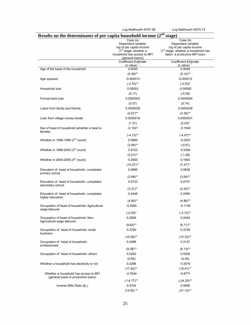
The second stage results where log of per capita household income is estimated are shown

in the second panel of Table 1. Most of the results are expected for Case (a) and Case (b).

Age of the head is positive and significant and its square is negative and significant.

Household size is non-significant. Among the loans from non-MFI sources, the coefficient

estimate of ‘loans from family and friends’ is positive and significant. As expected,

households headed by a female member tend to have much lesser per capita household

income, implying that female headed households are economically more disadvantaged than

male headed households. Year dummies show that per capita household income is the

smallest in a default case (1997-1998) and it is the largest in 2004-2005 after controlling for

inflation. The results of a set of dummy variables on educational achievement implies that a

household with the head least educated (or illiterate) tends to have the lowest per capita

household income and that with the head most highly educated (who completed higher

education) tends to have the highest level of income. Dummy variables on occupational

categories of head are also expected- a household headed by an agricultural wage labourer

has the lowest average per capita household income, while the household headed by a person

working as a professional or in small business has higher income. Infrastructure proxied by

19

electricity availability is positive and highly significant. Whether a household has access to

MFI (general loans or productive loans) is negative and significant, but this should not be

interpreted as a policy effect due to the sample selection bias. Treatment effects should be

derived by the equation (5) after controlling for the sample selection bias.

A summary of policy effects derived by treatment effects model and propensity score

matching (PSM) is presented in Table 2. Based on treatment effects model, we have derived

the treatment effects using the equation (5) for the panel data covering all the rounds and for

each round of cross-sectional data (i.e., for 1997-1998, 1998-1999, 1999-2000 and 2004-

2005). Regression results corresponding to the treatment effects based on each round of

cross-sectional data are broadly similar to those for panel data in Table 1 and are not

presented here.5 Average treatment effects for the treated (ATT) have been derived by PSM

using Nearest Neighbour Matching and Kernel Matching for each round of cross-sectional

data.6


We have found that simple household access to general loans from MFIs did not increase

log per capita household income significantly as the average treatment effect for panel data is

negative and non-significant as shown by the first row of the first panel, Case (a). However,

it is confirmed by the same panel data that household access to loans for productive purposes

from MFIs significantly increased log per capita household income as in the first row of the

second panel, Case (b). This suggests that monitoring how clients use the loans is important

for increasing household income, and thus decreasing poverty.

However, taking a close look at the policy effects derived by each cross-sectional

component of panel data, we have found that the policy effects have changed dramatically

over the years, positive and significant effects of MFI loans on per capita household income

20

in the first round in 1997-1998 to negative and significant, or non-significant effects in the

last round in 2004-2004 for both Case (a) and Case (b). That is, income-enhancing or

poverty-reducing effects of MFI loans have deteriorated over the years. It is also noted that a

broadly similar pattern of the results has been obtained by treatment effects model and PSM.

That is, the PSM has served as a robustness check.

In 1997-1998, the access to general loans from MFIs significantly increased per capita

household income Case (a) irrespective of whether we have used treatment effects model or

PSM, while in Case (b) the MFI loans for productive purposes significantly increased income

in the case of treatment effects model and of PSM when kernel matching is applied. That is,

the significant income enhancing effects were observed for both Cases (a) and (b) in 1997-

1998. In both 1998-1999 and 1999-2000, the policy effects of access to MFI general loans

became non-significant (Case (a)), whilst positive and significant effects were observed for

MFI productive loans (Case (b)) for both treatment effects model and PSM except the case of

PSM based on Nearest Neighbour Matching where the policy effect was positive and non-

significant. In contrast, in 2004-2005, the policy effect of MFI loans became negative and

significant in Case (a) (except the case of PSM based on Nearest Neighbour Matching where

it was positive and non-significant). In the same year, in Case (b), the policy effect of MFI

productive loans was negative and significant in the case where treatment effects model was

applied, whilst it is non-significant for PSM.

One could argue that there is a time lag from the time when a household member took

MFI loans for general purposes or productive purposes and the time when a household

actually enjoyed any income increase. For example, It may take a year or more for the

agricultural production assets purchased by productive loans from MFI to have any income

generating effects. Even if the MFI loan was used for consumption purposes, the household

income could increase in the long run if the loan was used to avoid the hardships arising from

21

short-run shocks, such as floods. Dercon and Christiansen (2008) showed using the Ethiopian

Household panel data that failure to reduce consumption fluctuations causes inefficiency in

agricultural production choices and increases the risk for the household trapped into chronic

poverty. Those who obtained MFI loans for productive purposes might see increase in the

household income in the future by the improved productivity, not necessarily observed at the

time when they obtained loans, but a year or a few years later.


Table 3 shows that the overall pattern of the results on the relationship between the lagged

MFI participation and log of per capita household income is not much different from those

for the current MFI participations presented in Table 2. However, in Case (a) where the MFI

participation is defined in terms of access to general loans, household access to MFI has a

significant and positive impact in 1998-1999 and 1999-2000 when treatment effects model is

employed. The results in the corresponding cases were non-significant in Table 2. Despite a

few changes, the results in Table 3 are broadly consistent with those in Table 2 and support

our conclusion that access to loans for productive purposes significantly increased log per

capita household income, but MFI loans for productive purposes did not and that the policy

effects of MFIs have deteriorated over the years.

Why the policy effects of MFIs have been weakened over the years is not clear. However,

it is surmised that severer competition among MFIs have made MFI loans more

commercialised, have squeezed the profits MFIs and have weakened the poverty-reducing

effects at household level in recent years after 2000. Another possibility is fungibility, that is,

some part of MFI loans was used for the purposes which do not increase income, such as

consumption. While the reasons are not obvious, our results suggest that more attention

should be drawn to the poverty reducing effects of microcredit and monitoring the purpose

and use of loans even in Bangladesh where microfinance has most flourished.

22

VI. Concluding Observations

The main purpose of the present study was to examine whether microfinance reduced poverty

in Bangladesh drawing upon the nationally representative household panel data covering 4

rounds, 1997-98, 1998-99, 1999-2000, and 2004-05. A special attention was drawn to the

issue of endogeneity by applying treatment effects model and propensity score matching

(PSM) for the participants and non-participants of microfinance programmes.

It has been confirmed by treatment effects model applied to panel data that household

access to loans for productive purposes from microfinance institutions (MFIs) significantly

increased per capita household income, while simple household access to general loans from

MFIs did not. The results will hold regardless of whether we define access to MFI loans in

terms of current access, or lagged access. This suggests that the monitoring of how clients

use the loans is important for increasing household income, and thus decreasing household

poverty. However, the application of treatment effects model and PSM to each cross-

sectional component of the panel data shows that (i) the policy effect of household access to

MFI general loans on per capita household income turned from positive and significant in

1997-1998 (and positive and significant in 1998-1999 and 1999-2000 in the cases of

treatment effects model where the access to loans from MFI is lagged) to negative and

significant in 2004-2005 and (ii) the effect of household access to MFI loans for productive

purposes on per capita household income also turned from positive and significant in 1997-

1998, 1998-1999, and 1999-2000 to negative and significant (in case of treatment effects

model) or non-significant (in case of PSM) in 2004-2005. Why the income enhancing or

poverty reducing effects became weak in 2004-2005 was not clear, but our results suggest

that a greater attention should be drawn to guaranteeing the sizable poverty reducing effects

through the MFI’s better systems of monitoring of loan usages in the situations where the

23

profits of MFIs became increasingly squeezed and their activities became more

commercialised under severe competitions among MFIs in recent years.

24

Table 1. Regression Results of Treatment Effects Model Results of Probit model on the determinants of participation in microfinance programme (1st stage)

Case (a) Dependent variable: whether a household has access to MFI

Case (b) Dependent variable: whether a

household has taken a productive MFI loan

Coefficient Estimate (z value) *1


Age of the head of the hh 0.0497 0.0444

(8.18)** (6.84)**

Age_squared -0.0005 -0.00049

(-8.92)** (-7.47)**

Household size 0.0200 0.0153

(4.21)** (3.08)**

Formal bank loan -0.0000054 -0.0000037

(-1.72)† (1.12)

Loans from family and friends -0.0000020 -0.0000027

(-1.93)† (2.21)*

Loan from village money lender -0.00000643 -0.0000013

(-2.84)** (-0.57)

Distance from nearest Upazilla (a business hub) -0.0078 -0.0048

(an instrument) (-3.74)** (-2.25)*

Sex of head of household (whether a head is female) 0.2054 0.1884

(3.53)** (3.02)**

Whether in 1998-1999 (2nd round) -0.0900 -0.2994

(-2.52)* (-8.34)**

Whether in 1999-2000 (3rd round) -0.2237 -0.5516

(-6.28)** (-15.04)**

Whether in 2004-2005 (4th round) -0.3072 -0.4700

(-7.92)** (-11.86)**

Education of head of household– completed primary school

-0.0273 -0.0432

(-0.79) (-1.21)

Education of head of household– completed secondary school

-0.2513 -0.2351

(-7.17)** (-6.44)**

Education of head of household– completed higher education

-0.4511 -0.4438

(-5.76)** (-5.20)**

Occupation of head of household- Agricultural wage labourer

-0.0561 -0.2260

(-1.22) (-4.72)**

Occupation of head of household- Non-Agricultural wage labourer

0.1618 0.0194

(3.62)** (0.43)

Occupation of head of household- small business 0.3380 0.2817

(9.17)** (7.67)**

Occupation of head of household- professionals -0.0855 -0.2036

(-1.47) (-3.28)**

Occupation of head of household- others -0.0844 -0.1702

(-1.99)* (-3.79)**

Whether a household has electricity or not -0.1283 -0.0268

(-4.31)** (-0.87)

Constant -1.007 -1.12

(6.25) (6.58)

Observations 10163 10163

Joint Significant Test LR Chi2(20)=560.37** Prob> Chi2=0.0000

LR Chi2(20)=647.94** Prob> Chi2=0.0000

25

Log likelihood=-6747.09 Log likelihood=-6270.73

Results on the determinants of per capita household income (2nd stage) Case (a)

Dependent variable: log of per capita income

(1st stage: whether a household has access to MFI

(general loans))

Case (b) Dependent variable:

log of per capita income (1st stage: whether a household has

taken a productive MFI loan)



Age of the head of the household 0.0050 0.0049

(5.39)** (5.14)**

Age squared -0.000013 -0.000012

(-2.76)** (-2.53)*

Household size 0.00053 -0.00092

(0.17) (-0.29)

Formal bank loan 0.0000003 0.0000004

(0.57) (0.74)

Loans from family and friends 0.0000028 0.0000028

(4.67)** (4.36)**

Loan from village money lender 0.0000018 0.0000031

(1.31) (2.24)*

Sex of head of household (whether a head is female)

-0.1521 -0.1549

(-4.13)** (-4.07)**

Whether in 1998-1999 (2nd round) 0.0885 -0.0207

(3.99)** (-0.87)

Whether in 1999-2000 (3rd round) 0.0733 -0.0264

(3.21)** (-1.08)

Whether in 2004-2005 (4th round) 0.2583 0.1954

(10.27)** (7.47)**

Education of head of household– completed primary school

0.0885 0.0836

(3.99)** (3.64)**

Education of head of household– completed secondary school

0.0733 0.0757

(3.21)** (3.25)**

Education of head of household– completed higher education

0.2446 0.2490

(4.90)** (4.86)**

Occupation of head of household- Agricultural wage labourer

-0.0594 -0.1145

(-2.00)* (-3.72)**

Occupation of head of household- Non-Agricultural wage labourer

0.2826 0.2404

(9.83)** (8.11)**

Occupation of head of household- small business

0.3790 0.3746

(15.65)** (15.33)**

Occupation of head of household- professionals

0.3488 0.3137

(9.38)** (8.13)**

Occupation of head of household- others 0.0255 0.0026

(0.95) (0.09)

Whether a household has electricity or not 0.3296 0.3579

(17.45)** (18.41)**

Whether a household has access to MFI (general loans or productive loans)

-0.7634 -0.8771

(-14.77)** (-24.20)**

Inverse Mills Ratio (βλ ) 0.4704 0.5695

(14.95) ** (27.12)**

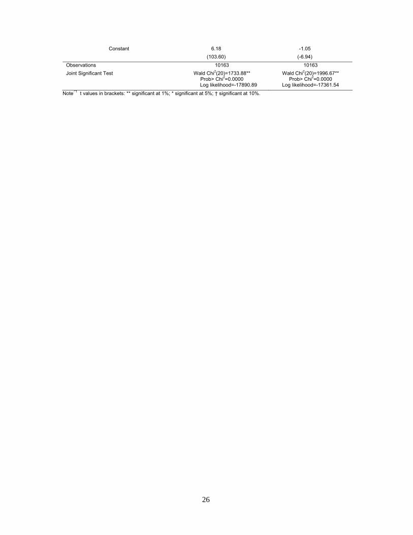
26

Constant 6.18 -1.05

(103.60) (-6.94)

Observations 10163 10163

Joint Significant Test Wald Chi2(20)=1733.88** Prob> Chi2=0.0000

Wald Chi2(20)=1996.67** Prob> Chi2=0.0000

Log likelihood=-17890.89 Log likelihood=-17361.54

Note:*1 t values in brackets: ** significant at 1%; * significant at 5%; † significant at 10%.

27

Table 2 Policy Effects (current effects) of Microfinance on per capita household income: Derived by Treatment Effects Model and Propensity Score Matching Case (a) Whether a household has access to MFI loans

Log per caita Household Income (mean) Policy Effect (t value) *1, 2 No. of obs.

(A-B)

Model With access to Without access to ATT: Average

MFI loans: A MFI loans: B treatment

effect

Panel Data

Treatment Effects Model 6.2077 6.2104 -0.0027 (-0.60) 10162

Cross-sectional Data

1997-1998 Treatment Effects Model 6.0767 6.0176 0.0591 (7.01)** 2580

PSM (Nearest Neighbour

Matching) - - 0.1000 (2.14)* Treat: 1515, Control: 672

PSM (Kernel Matching) - - 0.0690 (2.44)* Treat: 1515,

Control: 1061

1998-1999 Treatment Effects Model 6.1276 6.1362 -0.0085 (-1.07) 2602


Matching) - - 0.0170 (0.39) Treat: 1444, Control: 707

PSM (Kernel Matching) - - 0.0090 (0.31) Treat: 1444,

Control: 1150

1999-2000 Treatment Effects Model 6.2308 6.2254 0.0054 (0.64) 2619


Matching) - - -0.0110 (-0.25) Treat: 1318, Control: 685


Control: 1295

2004-2005 Treatment Effects Model 6.4000 6.4950 -0.0945 (-10.58)** 2594


Matching) - - -0.0610 (-1.43) Treat: 1194, Control: 704

PSM (Kernel Matching) - - -0.0770 (-2.92)** Treat: 1194,

Control: 1387

Notes: *1. t value is calculated by Bootstrapped Standard Errors for PSM.

*2 t values in brackets: ** significant at 1%; * significant at 5%. Case (b) Whether a household has access to MFI productive loans

Log per caita Household Income (mean)

Policy Effect (t value) *1, 2

No. of observations

(A-B)


MFI loans MFI loans treatment

effect

Panel Data

Treatment Effects Model 6.2501 6.1851 0.0649 (14.20)** 10162

Cross-sectional Data


PSM (Nearest Neighbour Matching) - - 0.0530 (1.27) Treat: 1218, Control: 714

PSM (Kernel Matching) - - 0.0780 (2.96)** Treat: 1218,

Control: 1357


PSM (Nearest Neighbour Matching) - - 0.0680 (1.40) Treat: 937,

Control: 667

28


Control: 1655


PSM (Nearest Neighbour Matching) - - 0.0860 (1.73)† Treat: 717,

Control: 601


Control: 1894



Control: 634

PSM (Kernel Matching) - - -0.0290 (-1.01) Treat: 770,

Control: 1812


*2 t values in brackets: ** significant at 1%; * significant at 5%; † significant at 10%.

29

Table 3 Policy Effects (lagged effects) of Microfinance on per capita household income: Derived by Treatment Effects Model and Propensity Score Matching

(a) Whether a househod has access to MFI loans



No. of observations

(A-B)


MFI loans: A MFI loans: B treatment

effect Panel Data

Treatment Effects Model 6.2597 6.2634 -0.0040 (-0.79) 7494

Cross-sectional Data 1998-1999 Treatment Effects Model 6.1455 6.1150 0.0304 (3.754)** 2554


Control: 1043

PSM (Kernel Matching) - - 0.0480 (1.48) Treat: 1507, Control: 675

1999-2000 Treatment Effects Model 6.2344 6.2187 0.0157 (2.06)* 2570

PSM (Nearest Neighbour Matching) - - 0.0370 (0.82) Treat: 1433, Control: 718


Control: 1133


PSM (Nearest Neighbour Matching) - - -0.0490 (-1.06) Treat: 1205, Control: 669


Control: 1154


*2 t values in brackets: ** significant at 1%; * significant at 5%; + significant at 10%.

(b) Whether a househod has access to MFI productive loans



No. of observations

(A-B)


MFI loans MFI loans treatment

effect Panel Data

Treatment Effects Model 6.2823 6.2517 0.0307 (5.90)** 7494

Cross-sectional Data 1998-1999 Treatment Effects Model 6.1497 6.1188 0.0308 (3.79)** 2554

PSM (Nearest Neighbour Matching) - - 0.0270 (0.62) Treat: 1208, Control:689

PSM (Kernel Matching) - - 0.0490 (1.44) Treat: 1208, Control:1340



Control: 676

PSM (Kernel Matching) - - 0.0490 (1.65)† Treat: 930,

Control: 1630



30

Control: 585


Control: 1725


*2 t values in brackets: ** significant at 1%; * significant at 5%; † significant at 10%.

31

Appendix Variable With access to MFI Without access to MFI With access to MFI loan for

Productive Purposes Without access to MFI laon for Productive purposes

Obs Mean Std. Dev. Obs Mean Std. Dev. Obs Mean Std. Dev. Obs Mean Std. Dev.

Age of Head of HH (age)

Pooled 5526 45.40 12.38 4954 47.32 15.50 3675 45.17 12.17 6805 46.93 14.82

Round 1 1545 43.86 12.28 1078 45.42 14.77 1237 43.73 12.07 1386 45.19 14.42

Round 2 1463 44.70 12.41 1170 46.62 14.49 948 44.53 12.11 1685 46.12 14.05

Round 3 1327 45.85 12.47 1312 47.26 14.25 721 45.55 12.32 1918 46.93 13.77

Round 4 1209 47.80 12.03 1420 49.43 17.56 778 47.82 11.79 1851 49.04 16.53

Sex of Head of HH (sex_hh)

Pooled 5528 0.95 0.22 4957 0.92 0.27 3676 0.95 0.21 6809 0.93 0.26

Round 1 1545 0.96 0.20 1078 0.93 0.25 1237 0.96 0.20 1386 0.94 0.25

Round 2 1463 0.95 0.21 1170 0.94 0.24 948 0.96 0.19 1685 0.94 0.24

Round 3 1327 0.95 0.20 1312 0.93 0.24 721 0.96 0.18 1918 0.94 0.23

Round 4 1209 0.93 0.29 1422 0.89 0.37 779 0.93 0.32 1852 0.90 0.35

Size of the HH (hh_size)

Pooled 5528 6.23 2.75 4957 6.27 3.16 3676 6.21 2.83 6809 6.27 3.02

Round 1 1545 5.73 2.20 1078 5.52 2.44 1237 5.66 2.12 1386 5.62 2.45

Round 2 1463 5.88 2.28 1170 5.88 2.60 948 5.82 2.26 1685 5.92 2.52

Round 3 1327 6.08 2.34 1312 6.10 2.66 721 6.08 2.37 1918 6.09 2.55

Round 4 1211 7.42 3.78 1423 7.32 4.08 779 7.66 4.05 1855 7.25 3.90

Dependency ratio (d_ratio)

Pooled 5526 0.98 0.70 4944 0.94 0.77 3676 0.97 0.69 6794 0.96 0.76

Round 1 1545 0.98 0.68 1076 0.88 0.68 1237 0.98 0.68 1384 0.91 0.68

Round 2 1463 0.99 0.67 1169 0.92 0.67 948 0.98 0.66 1684 0.94 0.68

Round 3 1327 0.93 0.66 1311 0.88 0.65 721 0.93 0.66 1917 0.89 0.65

Round 4 1209 1.02 0.81 1414 1.07 0.96 779 1.00 0.78 1844 1.07 0.95

Per capita Income (pcy)

Pooled 5528 638.15 1224.67 4957 823.70 2541.04 3676 664.04 1420.76 6809 759.24 2199.64

Round 1 1545 541.48 485.61 1078 579.27 623.34 1237 552.64 506.98 1386 560.90 579.90

Round 2 1463 577.15 647.30 1170 677.01 771.89 948 604.84 725.24 1685 630.84 696.55

Round 3 1327 633.41 1349.08 1312 701.10 762.11 721 688.43 1785.16 1918 659.03 678.64

32

Variable With access to MFI Without access to MFI With access to MFI loan for Productive Purposes

Without access to MFI laon for Productive purposes


Round 4 1211 826.00 2006.94 1423 1225.70 4578.39 779 875.71 2347.42 1855 1111.76 4053.84

Log of per capita income (lpcy))

Pooled 5528 6.17 0.71 4957 6.26 0.86 3676 6.19 0.71 6809 6.22 0.83

Round 1 1545 6.05 0.70 1078 6.02 0.86 1237 6.07 0.70 1386 6.01 0.82

Round 2 1448 6.10 0.76 1154 6.17 0.86 940 6.15 0.73 1662 6.12 0.84

Round 3 1324 6.19 0.67 1302 6.24 0.80 720 6.24 0.66 1906 6.20 0.76

Round 4 1211 6.38 0.66 1423 6.52 0.86 779 6.41 0.67 1855 6.48 0.82

Productive NGO loans (nl_prod)

Pooled 5528 8274.55 21739.83 4957 105.41 1822.62 3676 12585.50 25687.42 6809 0.00 0.00

Round 1 1545 18505.53 37656.36 1078 200.92 3574.95 1237 23288.32 40838.83 1386 0.00 0.00

Round 2 1463 4139.04 5639.96 1170 124.60 1067.35 948 6541.35 5845.09 1685 0.00 0.00

Round 3 1327 3396.04 5156.92 1312 44.38 563.57 721 6331.19 5538.54 1918 0.00 0.00

Round 4 1211 5488.87 9716.99 1423 71.63 810.70 779 8663.62 10945.31 1855 0.00 0.00

Non-productive NGO loans (nl_nprod)

Pooled 5528 2574.08 13832.51 4957 24.77 440.40 3676 2368.82 15820.98 6809 828.98 4693.11

Round 1 1545 3267.84 17997.61 1078 11.64 307.84 1237 2620.46 17846.45 1386 1313.02 8999.78

Round 2 1463 2357.83 4113.11 1170 35.25 427.70 948 2329.26 3814.28 1685 761.20 2798.14

Round 3 1327 2328.31 19663.10 1312 7.69 220.83 721 2652.60 26393.51 1918 619.00 2560.33

Round 4 1211 2238.30 4234.92 1423 41.40 638.83 779 1730.95 3664.54 1855 766.08 2794.69

Formal bank loans (fbl_tot)

Pooled 5528 376.26 3615.70 4957 848.57 20363.00 3676 385.46 4013.81 6809 715.14 17430.35

Round 1 1545 194.22 1735.18 1078 470.96 4132.29 1237 188.41 1496.01 1386 414.64 3827.35

Round 2 1463 396.77 2712.55 1170 772.65 4667.90 948 409.32 2621.24 1685 650.70 4205.15

Round 3 1327 369.17 2516.35 1312 1562.59 38801.45 721 280.31 2294.18 1918 1218.93 32128.97

Round 4 1211 596.65 6329.83 1423 585.94 5232.52 779 777.59 7698.03 1855 512.45 4718.14

Loans from friends and family (ffl_tot)

Pooled 5528 2258.52 10024.06 4957 2970.09 16144.27 3676 2138.78 10314.13 6809 2841.20 14625.54

Round 1 1545 2515.75 11259.95 1078 3300.98 13033.71 1237 2513.46 11988.29 1386 3128.52 12053.55

Round 2 1463 2571.42 9321.90 1170 3816.14 18025.69 948 2226.29 8493.35 1685 3629.88 16134.47

Round 3 1327 2410.36 8732.30 1312 3938.79 22638.89 721 2381.82 8815.89 1918 3466.60 19353.00

Round 4 1211 1516.01 10961.81 1423 1201.90 6336.88 779 1416.42 11523.49 1855 1316.87 7316.42

33

Variable With access to MFI Without access to MFI With access to MFI loan for Productive Purposes

Without access to MFI laon for Productive purposes


Loans from village money lenders (vml_tot)

Pooled 5528 486.51 4301.19 4957 818.06 7443.37 3676 624.81 5101.62 6809 653.22 6429.93

Round 1 1545 561.08 5036.03 1078 737.06 7547.03 1237 608.50 5477.44 1386 655.63 6767.78

Round 2 1463 408.36 2714.25 1170 1095.08 9792.01 948 515.43 3205.77 1685 824.95 8205.16

Round 3 1327 351.79 3588.69 1312 613.10 4468.81 721 523.48 4514.05 1918 466.00 3864.57

Round 4 1211 642.73 5420.97 1423 849.58 7281.99 779 896.08 6655.58 1855 695.01 6423.82

Distance to nearest Upzilla (dist_uz)

Pooled 5526 7.38 6.03 4956 7.71 6.28 3674 7.40 5.97 6808 7.61 6.25

Round 1 1545 7.18 5.83 1078 8.06 6.58 1237 7.40 5.85 1386 7.67 6.43

Round 2 1463 7.29 5.97 1170 7.83 6.38 948 7.36 5.98 1685 7.62 6.25

Round 3 1327 7.28 5.98 1312 7.79 6.32 721 7.41 6.03 1918 7.57 6.20

Round 4 1209 7.80 6.37 1422 7.28 5.92 777 7.41 6.10 1854 7.57 6.15

whether household has electricity or not (elec_hh)

Pooled 5503 0.27 0.44 4944 0.34 0.47 3662 0.28 0.45 6785 0.32 0.46

Round 1 1537 0.25 0.43 1074 0.26 0.44 1231 0.24 0.43 1380 0.26 0.44

Round 2 1455 1.77 0.42 1166 1.71 0.45 944 1.76 0.42 1677 1.73 0.44

Round 3 1326 1.74 0.43 1312 1.66 0.47 721 1.73 0.44 1917 1.69 0.46

Round 4 1203 1.63 0.48 1418 1.56 0.50 775 1.60 0.49 1846 1.59 0.49

34

Endnotes 1 It is noted that joint liability payment may not be imposed on the group, for example, in case of lending by Grameen Bank, but repayment performance of the group is closely monitored by the communities and the Bank. To maintain reputations in the community, a member has an incentive to build skills and work hard to keep repaying the instalments. See definitions and salient features of microcredit at http://www.grameen-info.org/index.php?option=com_content&task=view&id=28&Itemid=108 (accessed on 30th September 2010). 2 There are two hypotheses necessary for validating PSM, (i) Balancing Hypothesis, related to balancing of pre-treatment variables given the propensity score, which implies that given a specific probability of having access to MFI, a vector of household characteristics, is uncorrelated to the access to MFI and (ii) Unconfoundedness Hypothesis which postulates that given a propensity score, log per capita household income is uncorrelated to the access to a MFI (Rosenbaun and Rubin, 1983). 3 We did not use Radius Matching as the results are sensitive to the predetermined radius.

4 The possibility cannot be ruled out that the household decisions to take loans from the traditional sources or to take loans from MFIs are made simultaneously and thus these variables may not be entirely exogenous. It has been found that dropping these variables will not change the final results dramatically. We have decided to keep these variables to put more importance on avoiding any bias from omitting these important explanatory variables, the factors which had long existed well before microfinace programmes were implemented. 5 Regression results will be furnished on request. 6 PSM is not applied for the panel data because of the difficulty in matching the data over the years. We have used logit model in the first stage which shows a broadly similar pattern of the results to those derived by probit model presented in Table 1.

35

References

Ahlin, C. and Townsend, R. (2007) Using Repayment Data to Test Across Models of Joint

Liability Lending, The Economic Journal, 117, pp. F11-F51.

Ahmed S. (2007) Microfinance Programmes in Bangladesh: Experiences and Issues, in I.

Simorangkir (ed.) Macroeconomic Stability towards high Growth and

Employment. :Proceedings on an International seminar held in Denpasar (Bali:

Indonesia).

Armendáriz, B., and Morduch, J. (2005) The Economics of Microfinance (Cambridge, MA:

The MIT Press).

Banerjee, A., Duflo, E., Glennerster, R. and Kinnan, C. (2009) The Miracle of Microfinance?

Evidence from a Randomised Evaluation, Department of Economics, Massachusetts

Institute of Technology (MIT) Working Paper, May 2009.

Bateman, M., and Chang, H. (2009) The Microfinance Illusion, mimeo., Cambridge, Faculty

of Economics, University of Cambridge, available from

http://www.econ.cam.ac.uk/faculty/chang/pubs/Microfinance.pdf.

Becker, S. and Ichino, A. (2002) Estimation of Average Treatment Effects based on

Propensity Scores, The Stata Journal, 2(4), pp.358-377.

Besley, T., and Coate, S. (1995) Group lending, repayment incentives and social collateral,

Journal of Development Economics, 46 (1), pp.1-18.

BBS (2008) Report On The Household Income and Expenditure Survey 2005 (Dhaka:

Bangladesh Bureau of Statistics).

Dehejia, R. (2005) Practical Propensity Score Matching: a Reply to Smith and Todd, Journal

of Econometrics, 125, pp.355-364.

Dehejia, R. and Wahba, S. (2002) Propensity Score Matching Methods for Nonexperimental

Causal Studies, Review of Economics and Statistics, 84 (1), pp.151-161.

36

Dercon, C., and Christiansen, L. (2008) Consumption risk, technology adoption and poverty

traps: evidence from Ethiopia, World Economy & Finance Research Programme Working

Paper Series WEF0035, University of London, Birkbeck.

Ehrbeck, T. (2006) Optimizing capital supply in support of microfinance industry growth.

Presentation at microfinance investor roundtable, Washington, DC, October 24-25.

McKinsey&Co.

Farashuddin, F. and Amin, N. (1998) Poverty Alleviation and Empowerment: An Impact

Assessment Study of BRAC's RDP - Ten Qualitative Case Studies. Mimeo, (Dhaka:

BRAC Research and Evaluation Division).

Foster, M. (2003). Propensity Score Matching: An Illustrative Analysis of Dose Response,

Medical Care, 41(10), pp.1183-1192.

Greene, W. H. (2003). Econometric Analysis 5th Edition (Upper Saddle River, NJ: Prentice-

Hall).

Heckman, J. (1979). Sample selection bias as a specification error, Econometrica, 47, pp.153-

161.

Hulme, D. and P. Mosley (1996). Finance against Poverty. Routledge, London.

Imai, K. S., Arun, T. and Annim, S. K. (2010) Microfinance and Household Poverty

Reduction: New evidence from India, World Development, forthcoming.

Karlan, D. and Zinman, J. (2009) Expanding Microenterprise Credit Access: Using

Randomized Supply Decisions to Estimate the Impacts in Manila. Working Paper. Yale

University, Dartmouth College, and Innovations for Poverty Action.

Khandker, S. R. (2005) Microfinance and Poverty: Evidence Using Panel Data from

Bangladesh, The World Bank Economic Review, 19(2), pp.263-286.

Maddala, G. S. (1983) Limited dependent and qualitative variables in econometrics

(Cambridge, Cambridge University Press).

37

Montgomery R., D. Bhattacharya and D. Hulme (1996) Credit for the Poor in Bangladesh:

The BRAC Rural Development Programme and the Government Thana Resource

Development and Employment Programme, in D. Hulme and P. Mosely, Finance against

Poverty. Vols. I and 2 (London: Routledge).

Morduch, J. (1998) Does Microfinance Really Help the Poor: New Evidence from Flagship

Programs in Bangladesh, Mimeo, Department of Economics and HIID, Harvard

University and Hoover Institution, Stanford University.

Pitt, M., and Khandker, S. R. (1998) The Impact of Group-Based Credit on Poor Households

in Bangladesh: Does the Gender of Participants Matter?, Journal of Political Economy,

106(5), pp.958–96.

PKSF (2006) MAPs on Microcredit Coverage in Upazilas of Bangladesh (Dhaka, Bangladesh,

Palli Karma Sahayak Foundation).

Pollin, R. (2007) Microcredit: False Hopes and Real Possibilities. Foreign Policy Focus,

available from http://www.fpif.org/fpiftxt/4323.

Ravallion, M. (2008) Evaluating Anti-Poverty Programme, Chapter 59 in Handbook of

Development Economics, Volume 4, P. Schultz and J. Strauss (eds) (New York: North

Holland) .

Roodman, D., and J. Morduch (2009) The Impact of Microcredit on the Poor in Bangladesh:

Revisiting the Evidence, CGD Working Paper 174 (Washington, D.C.: Center for Global

Development).

Rosenbaum, P. R., and Rubin, D. B. (1983) The Central Role of the Propensity Score in

Observational Studies for Causal Effects, Biometrica, 70(1), pp.41-55.

Smith, J. A., and Todd, P. E. (2005) Does Matching Overcome LaLonde’s Critique of

Nonexperimental Estimators?, Journal of Econometrics, 125, pp.305-353.

38

Todd, P. E. (2008). ‘Evaluating Social Programs with Endogenous Program Placement and

Selection of the Treated’, Chapter 60 in Handbook of Development Economics, Volume 4,

P. Schultz and J. Strauss (eds) (New York, North-Holland).

Wood, G. and Sharif, I. (eds) (1997) Who needs credit? Poverty and finance in Bangladesh.

(London, Zed Books).

Zaman, H. (1998) Who benefits and to what extent? An evaluation of BRAC's micro-credit

program, University of Sussex, D.Phil thesis.

Documents

Katsushi Imai Md. Shafiul Azam - University of Manchesterhummedia.manchester.ac.uk/schools/soss/economics/discussionpaper… · 1 Does Microfinance Reduce Poverty in Bangladesh? New