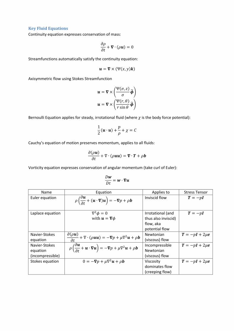
Key Fluid Equations

Continuity equation expresses conservation of mass:

Streamfunctions automatically satisfy the continuity equation:

Axisymmetric flow using Stokes Streamfunction

Bernoulli Equation applies for steady, irrotational fluid (where is the body force potential):

Cauchy’s equation of motion preserves momentum, applies to all fluids:

Vorticity equation expresses conservation of angular momentum (take curl of Euler):

Name Equation Applies to Stress Tensor

Euler equation

Inviscid flow

Laplace equation

Irrotational (and thus also inviscid) flow, aka potential flow

Navier-Stokes equation

Newtonian (viscous) flow

Navier-Stokes equation (incompressible)

Incompressible Newtonian (viscous) flow

Stokes equation Viscosity dominates flow (creeping flow)

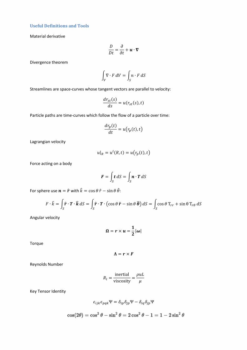
Useful Definitions and Tools

Material derivative

Divergence theorem

Streamlines are space-curves whose tangent vectors are parallel to velocity:

Particle paths are time-curves which follow the flow of a particle over time:

Lagrangian velocity

Force acting on a body

For sphere use with :

Angular velocity

Torque

Reynolds Number

Key Tensor Identity

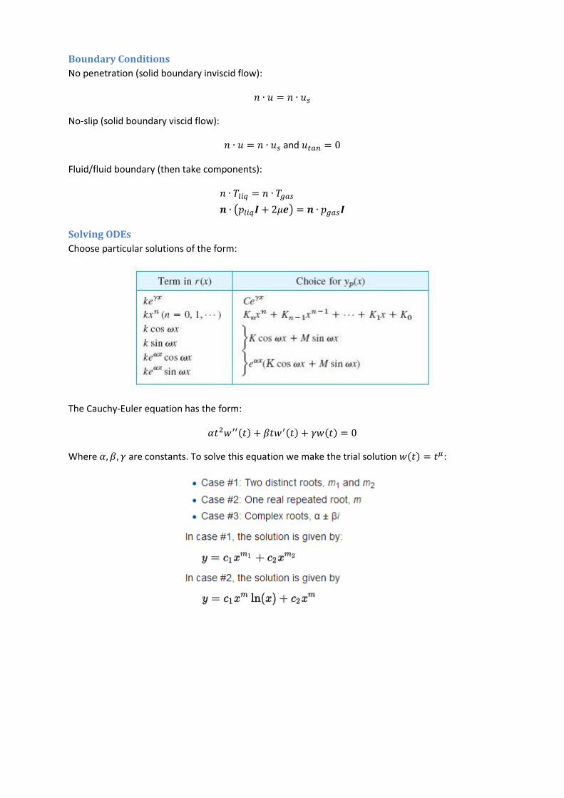
Boundary Conditions

No penetration (solid boundary inviscid flow):

No-slip (solid boundary viscid flow):

and

Fluid/fluid boundary (then take components):

Solving ODEs

Choose particular solutions of the form:

The Cauchy-Euler equation has the form:

Where are constants. To solve this equation we make the trial solution :

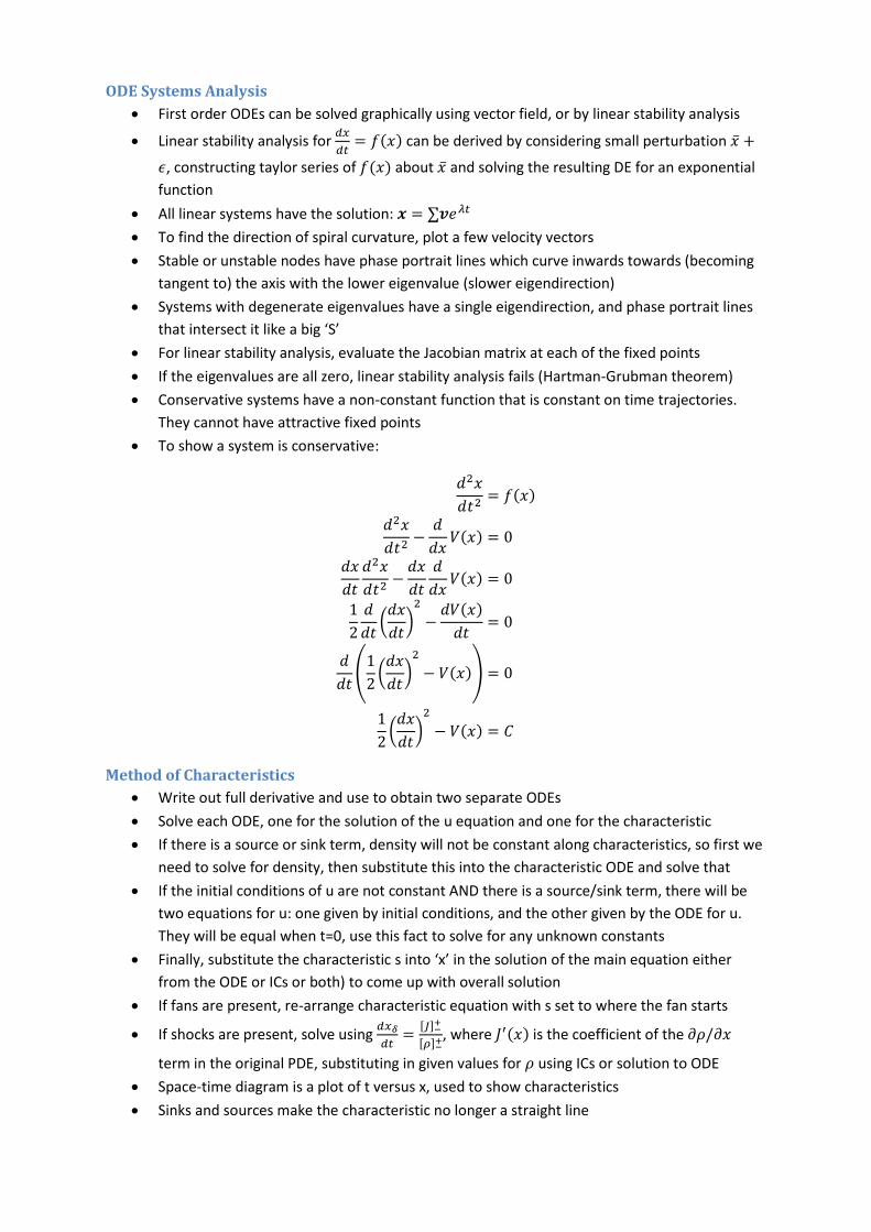
ODE Systems Analysis

First order ODEs can be solved graphically using vector field, or by linear stability analysis

Linear stability analysis for

can be derived by considering small perturbation

, constructing taylor series of about and solving the resulting DE for an exponential

function

All linear systems have the solution:

To find the direction of spiral curvature, plot a few velocity vectors

Stable or unstable nodes have phase portrait lines which curve inwards towards (becoming

tangent to) the axis with the lower eigenvalue (slower eigendirection)

Systems with degenerate eigenvalues have a single eigendirection, and phase portrait lines

that intersect it like a big ‘S’

For linear stability analysis, evaluate the Jacobian matrix at each of the fixed points

If the eigenvalues are all zero, linear stability analysis fails (Hartman-Grubman theorem)

Conservative systems have a non-constant function that is constant on time trajectories.

They cannot have attractive fixed points

To show a system is conservative:

Method of Characteristics

Write out full derivative and use to obtain two separate ODEs

Solve each ODE, one for the solution of the u equation and one for the characteristic

If there is a source or sink term, density will not be constant along characteristics, so first we

need to solve for density, then substitute this into the characteristic ODE and solve that

If the initial conditions of u are not constant AND there is a source/sink term, there will be

two equations for u: one given by initial conditions, and the other given by the ODE for u.

They will be equal when t=0, use this fact to solve for any unknown constants

Finally, substitute the characteristic s into ‘x’ in the solution of the main equation either

from the ODE or ICs or both) to come up with overall solution

If fans are present, re-arrange characteristic equation with s set to where the fan starts

If shocks are present, solve using

, where is the coefficient of the

term in the original PDE, substituting in given values for using ICs or solution to ODE

Space-time diagram is a plot of t versus x, used to show characteristics

Sinks and sources make the characteristic no longer a straight line