Embed Size (px)
Citation preview
Kinematic Model of Robot Manipulators
Claudio Melchiorri
Dipartimento di Ingegneria dell’Energia Elettrica e dell’Informazione (DEI)
Universita di Bologna
email: [email protected]
C. Melchiorri (DEIS) Kinematic Model 1 / 164
Summary
1 Kinematic Model
2 Direct Kinematic Model
3 Inverse Kinematic Model
4 Differential Kinematics
5 Statics - Singularities - Inverse differential kinematics
6 Inverse kinematics algorithms
7 Measures of performance
C. Melchiorri (DEIS) Kinematic Model 2 / 164
Kinematic Model Introduction
Kinematic Model
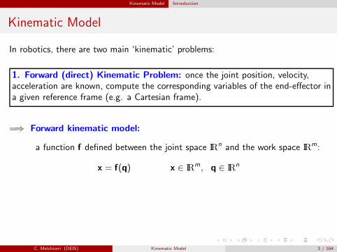
In robotics, there are two main ‘kinematic’ problems:
1. Forward (direct) Kinematic Problem: once the joint position, velocity,acceleration are known, compute the corresponding variables of the end-effector ina given reference frame (e.g. a Cartesian frame).
=⇒ Forward kinematic model:
a function f defined between the joint space IRn and the work space IR
m:
x = f(q) x ∈ IRm, q ∈ IR
n
C. Melchiorri (DEIS) Kinematic Model 3 / 164
Kinematic Model Introduction
Kinematic Model
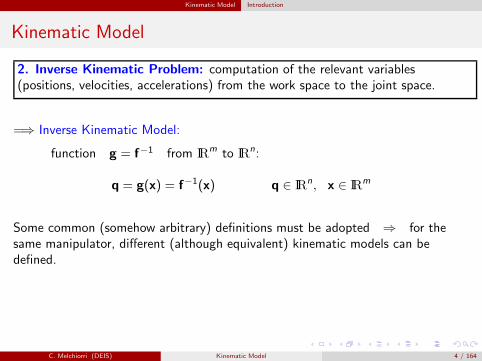
2. Inverse Kinematic Problem: computation of the relevant variables(positions, velocities, accelerations) from the work space to the joint space.
=⇒ Inverse Kinematic Model:
function g = f−1 from IRm to IR
n:
q = g(x) = f−1(x) q ∈ IRn, x ∈ IR
m
Some common (somehow arbitrary) definitions must be adopted ⇒ for thesame manipulator, different (although equivalent) kinematic models can bedefined.
C. Melchiorri (DEIS) Kinematic Model 4 / 164
Kinematic Model Introduction
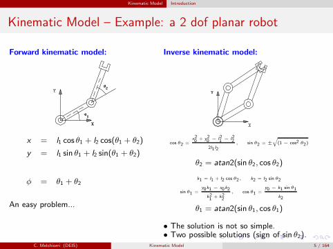
Kinematic Model – Example: a 2 dof planar robot
Forward kinematic model:
x = l1 cos θ1 + l2 cos(θ1 + θ2)
y = l1 sin θ1 + l2 sin(θ1 + θ2)
φ = θ1 + θ2
An easy problem...
Inverse kinematic model:
cos θ2 =x20 + y20 − l21 − l22
2l1l2
, sin θ2 = ±
√
(1 − cos2 θ2)
θ2 = atan2(sin θ2, cos θ2)
k1 = l1 + l2 cos θ2, k2 = l2 sin θ2
sin θ1 =y0k1 − x0k2
k21
+ k22
, cos θ1 =y0 − k1 sin θ1
k2
θ1 = atan2(sin θ1, cos θ1)
• The solution is not so simple.• Two possible solutions (sign of sin θ2).
C. Melchiorri (DEIS) Kinematic Model 5 / 164
Kinematic Model Introduction
Kinematic Model
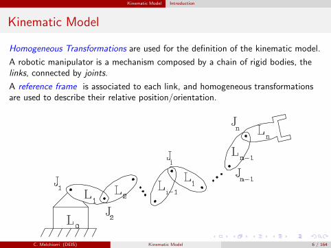
Homogeneous Transformations are used for the definition of the kinematic model.
A robotic manipulator is a mechanism composed by a chain of rigid bodies, thelinks, connected by joints.
A reference frame is associated to each link, and homogeneous transformationsare used to describe their relative position/orientation.
C. Melchiorri (DEIS) Kinematic Model 6 / 164
Kinematic Model Introduction
Kinematic Model
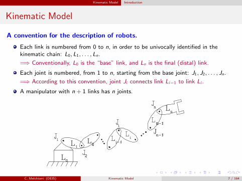
A convention for the description of robots.
Each link is numbered from 0 to n, in order to be univocally identified in thekinematic chain: L0, L1, . . . , Ln.
=⇒ Conventionally, L0 is the “base” link, and Ln is the final (distal) link.
Each joint is numbered, from 1 to n, starting from the base joint: J1, J2, . . . , Jn.
=⇒ According to this convention, joint Ji connects link Li−1 to link Li .
A manipulator with n + 1 links has n joints.
C. Melchiorri (DEIS) Kinematic Model 7 / 164
Kinematic Model Introduction
Kinematic Model
The motion of the joints changes the end-effector position/orientation in the workspace.
The position and the orientation of the end-effector result to be a (non linear)function of the n joint variables q1, q2, ..., qn, i.e.
p = f(q1, q2, ..., qn) = f(q)
q = [q1 q2 . . . qn]T is defined in the joint space IR
n,
p is defined in the work space IRm.
Usually, p is composed by:
some position components (e.g. x , y , z , wrt a Cartesian reference frame)
some orientation components (e.g. Euler or RPY angles).
C. Melchiorri (DEIS) Kinematic Model 8 / 164
Kinematic Model Denavit-Hartenberg Parameters
Kinematic Model
Need of defining a systematic and possibly unique method for the definition of thekinematic model of a robot manipulator:
DENAVIT-HARTENBERG NOTATION
A reference frame is assigned to each link, and homogeneous transformationsmatrices are used to describe the relative position/orientation of these frames.
The reference frames are assigned according to a particular convention, andtherefore the number of parameters needed to describe the pose of each link, andconsequently of the robot, is minimized.
C. Melchiorri (DEIS) Kinematic Model 9 / 164
Kinematic Model Denavit-Hartenberg Parameters
Denavit-Hartenberg Parameters
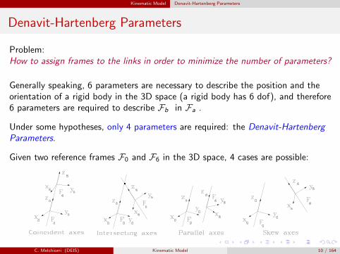
Problem:How to assign frames to the links in order to minimize the number of parameters?
Generally speaking, 6 parameters are necessary to describe the position and theorientation of a rigid body in the 3D space (a rigid body has 6 dof), and therefore6 parameters are required to describe Fb in Fa .
Under some hypotheses, only 4 parameters are required: the Denavit-HartenbergParameters.
Given two reference frames F0 and F6 in the 3D space, 4 cases are possible:
C. Melchiorri (DEIS) Kinematic Model 10 / 164
Kinematic Model Denavit-Hartenberg Parameters
Denavit-Hartenberg Parameters
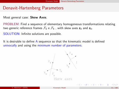
Most general case: Skew Axes.
PROBLEM: Find a sequence of elementary homogeneous transformations relatingtwo generic reference frames F0 e F6 , with skew axes z0 and z6.
SOLUTION: Infinite solutions are possible.
It is desirable to define A sequence so that the kinematic model is definedunivocally and using the minimum number of parameters.
C. Melchiorri (DEIS) Kinematic Model 11 / 164
Kinematic Model Denavit-Hartenberg Parameters
Denavit-Hartenberg Parameters - Procedure
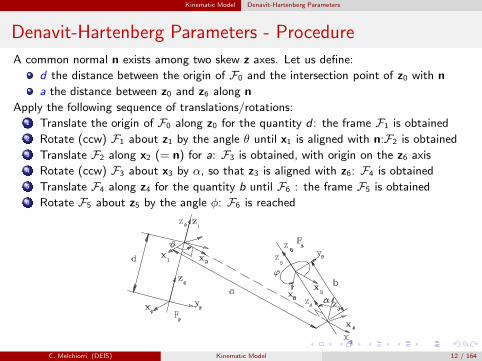
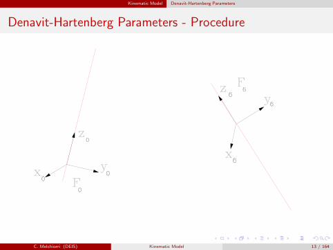
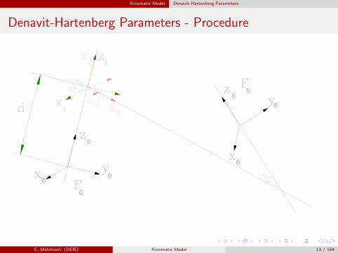
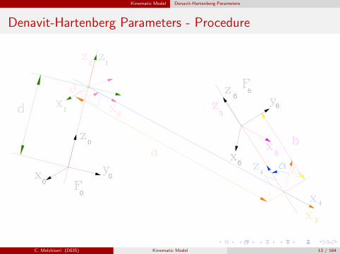
A common normal n exists among two skew z axes. Let us define:
d the distance between the origin of F0 and the intersection point of z0 with n
a the distance between z0 and z6 along n
Apply the following sequence of translations/rotations:1 Translate the origin of F0 along z0 for the quantity d : the frame F1 is obtained2 Rotate (ccw) F1 about z1 by the angle θ until x1 is aligned with n:F2 is obtained3 Translate F2 along x2 (= n) for a: F3 is obtained, with origin on the z6 axis4 Rotate (ccw) F3 about x3 by α, so that z3 is aligned with z6: F4 is obtained5 Translate F4 along z4 for the quantity b until F6 : the frame F5 is obtained6 Rotate F5 about z5 by the angle φ: F6 is reached
C. Melchiorri (DEIS) Kinematic Model 12 / 164
Kinematic Model Denavit-Hartenberg Parameters
Denavit-Hartenberg Parameters - Procedure
C. Melchiorri (DEIS) Kinematic Model 13 / 164

Kinematic Model Denavit-Hartenberg Parameters
Denavit-Hartenberg Parameters - Procedure
C. Melchiorri (DEIS) Kinematic Model 13 / 164

Kinematic Model Denavit-Hartenberg Parameters
Denavit-Hartenberg Parameters - Procedure
C. Melchiorri (DEIS) Kinematic Model 13 / 164
Kinematic Model Denavit-Hartenberg Parameters
Denavit-Hartenberg Parameters - Procedure
C. Melchiorri (DEIS) Kinematic Model 13 / 164

Kinematic Model Denavit-Hartenberg Parameters
Denavit-Hartenberg Parameters - Procedure
C. Melchiorri (DEIS) Kinematic Model 13 / 164

Kinematic Model Denavit-Hartenberg Parameters
Denavit-Hartenberg Parameters - Procedure
C. Melchiorri (DEIS) Kinematic Model 13 / 164
Kinematic Model Denavit-Hartenberg Parameters
Denavit-Hartenberg Parameters - Procedure
C. Melchiorri (DEIS) Kinematic Model 13 / 164

Kinematic Model Denavit-Hartenberg Parameters
Denavit-Hartenberg Parameters - Procedure
C. Melchiorri (DEIS) Kinematic Model 13 / 164
Kinematic Model Denavit-Hartenberg Parameters
Denavit-Hartenberg Parameters
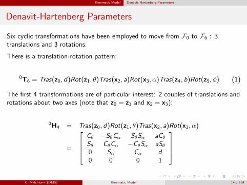
Six cyclic transformations have been employed to move from F0 to F6 : 3translations and 3 rotations.
There is a translation-rotation pattern:
0T6 = Tras(z0, d)Rot(z1, θ)Tras(x2, a)Rot(x3, α)Tras(z4, b)Rot(z5, φ) (1)
The first 4 transformations are of particular interest: 2 couples of translations androtations about two axes (note that z0 = z1 and x2 = x3):
0H4 = Tras(z0, d)Rot(z1, θ)Tras(x2, a)Rot(x3, α)
=
Cθ −SθCα SθSα aCθSθ CθCα −CθSα aSθ0 Sα Cα d0 0 0 1
C. Melchiorri (DEIS) Kinematic Model 14 / 164
Kinematic Model Denavit-Hartenberg Parameters
Denavit-Hartenberg Parameters
Matrix 0T6 can be expressed in terms of H matrices by adding to (1)
a null translation along x6, obtaining the frame F7
a null rotation about x7, obtaining the frame F8
Therefore we have
0T8 = Tras(z0, d)Rot(z1, θ)Tras(x2, a)Rot(x3, α)
Tras(z4, b)Rot(z5, φ)Tras(x6, 0)Rot(x7, 0)
that is expressed by cyclic transformations.
C. Melchiorri (DEIS) Kinematic Model 15 / 164
Kinematic Model Denavit-Hartenberg Parameters
Denavit-Hartenberg Parameters
If another frame F12 is given, it is possible to move from F6 to F12 by means of asequence similar to (1). Then, the transformation from F0 to F12 is
0T12 = 0H4 Tras(z4, b)Rot(z5, φ)Tras(z6, d′)Rot(z7, θ
′)Tras(x8, a′)Rot(x9, α
′)
Tras(z10, b′)Rot(z11, φ
′)Tras(x12, 0)Rot(x13, 0)
Since a translation and a rotation about the same axis may commute, i.e.
Rot(z5, φ)Tras(z6, d′) = Tras(z6, d
′)Rot(z5, φ)
we have that
Tras(z4, b)Rot(z5, φ)Tras(z6, d′)Rot(z7, θ
′) = Tras(z4, b)Tras(z6, d′)Rot(z5, φ)Rot(z7, θ
′)
= Tras(z4, b + d′)Rot(z5, φ+ θ′)
C. Melchiorri (DEIS) Kinematic Model 16 / 164
Kinematic Model Denavit-Hartenberg Parameters
Denavit-Hartenberg Parameters
In conclusion, the transformation between F0 and F12 is expressed by two DHtransformations expressed by H matrices:
the first one with parameters d , θ, a, α,
the second one with parameters (b + d ′), (φ+ θ′), a′, α′
(and a third one with parameters b′, φ′, 0, 0).
C. Melchiorri (DEIS) Kinematic Model 17 / 164
Kinematic Model Denavit-Hartenberg Parameters
Denavit-Hartenberg Parameters
In general, only frames F0 and F4 are of interest, and not the intermediate ones(F1 -F3 ). Therefore, F4 will be indicated from now as F1 . The transformation0H4 is then indicated as 0H1.
0H1 = Tras(z0, d)Rot(z1, θ)Tras(x2, a)Rot(x3, α)
=
Cθ −SθCα SθSα aCθSθ CθCα −CθSα aSθ0 Sα Cα d0 0 0 1
The frames associated to each link are used only for the definition of thekinematic model of the robot: usually their position/orientation may be freelyassigned and do not depend by other constraints.
Therefore, these frames are assigned in order to minimize the number ofparameters required for the definition of the kinematic model.
C. Melchiorri (DEIS) Kinematic Model 18 / 164
Kinematic Model Denavit-Hartenberg Parameters
Denavit-Hartenberg Parameters
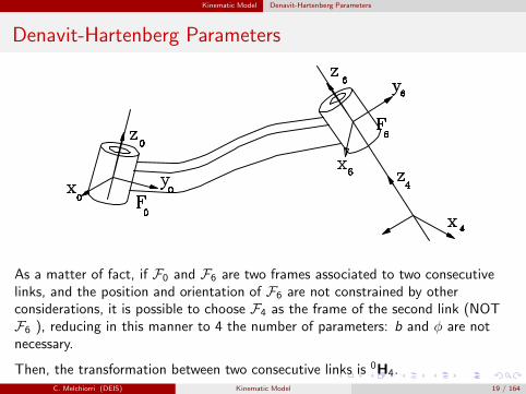
As a matter of fact, if F0 and F6 are two frames associated to two consecutivelinks, and the position and orientation of F6 are not constrained by otherconsiderations, it is possible to choose F4 as the frame of the second link (NOTF6 ), reducing in this manner to 4 the number of parameters: b and φ are notnecessary.
Then, the transformation between two consecutive links is 0H4.C. Melchiorri (DEIS) Kinematic Model 19 / 164
Kinematic Model Denavit-Hartenberg Parameters
Denavit-Hartenberg Parameters
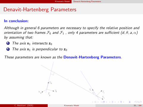
In conclusion:
Although in general 6 parameters are necessary to specify the relative position andorientation of two frames F0 and F1 , only 4 parameters are sufficient (d , θ, a, α)by assuming that:
1 The axis x1 intersects z02 The axis x1 is perpendicular to z0
These parameters are known as the Denavit-Hartenberg Parameters.
C. Melchiorri (DEIS) Kinematic Model 20 / 164
Kinematic Model Denavit-Hartenberg Parameters
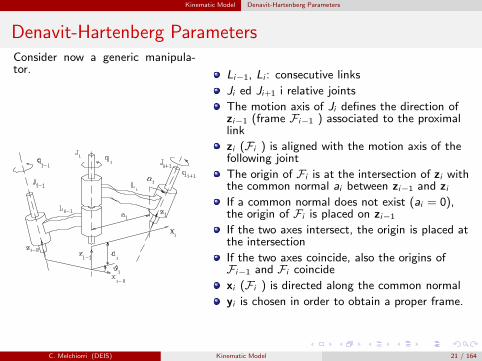
Denavit-Hartenberg ParametersConsider now a generic manipula-tor.
Li−1, Li : consecutive links
Ji ed Ji+1 i relative joints
The motion axis of Ji defines the direction ofzi−1 (frame Fi−1 ) associated to the proximallink
zi (Fi ) is aligned with the motion axis of thefollowing joint
The origin of Fi is at the intersection of zi withthe common normal ai between zi−1 and ziIf a common normal does not exist (ai = 0),the origin of Fi is placed on zi−1
If the two axes intersect, the origin is placed atthe intersection
If the two axes coincide, also the origins ofFi−1 and Fi coincide
xi (Fi ) is directed along the common normal
yi is chosen in order to obtain a proper frame.
C. Melchiorri (DEIS) Kinematic Model 21 / 164
Kinematic Model Denavit-Hartenberg Parameters
Denavit-Hartenberg Parameters
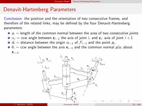
Conclusion: the position and the orientation of two consecutive frames, andtherefore of the related links, may be defined by the four Denavit-Hartenbergparameters:
ai = length of the common normal between the axes of two consecutive jointsαi = ccw angle between zi−1 the axis of joint i , and zi , axis of joint i + 1di = distance between the origin oi−1 of Fi−1 and the point pi ,θi = ccw angle between the axis xi−1 and the common normal ˆpioi aboutzi−1.
C. Melchiorri (DEIS) Kinematic Model 22 / 164
Kinematic Model Denavit-Hartenberg Parameters
Denavit-Hartenberg Parameters
The parameters ai and αi are constant and depend only on the link geometry:
ai is the link lengthαi is the link twist angle
between the joints’ axes.
Considering the two other parameters, depending on the joint type one isconstant and the other one may change in time:
prismatic joint: di is the joint variable and θi is constant;rotational joint: θi is the joint variable and di is constant.
C. Melchiorri (DEIS) Kinematic Model 23 / 164
Kinematic Model Denavit-Hartenberg Parameters
Denavit-Hartenberg Parameters
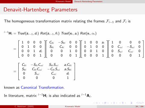
The homogeneous transformation matrix relating the frames Fi−1 and Fi is
i−1Hi = Trasl(zi−1, di) Rot(zi−1, θi) Trasl(xi , ai) Rot(xi , αi )
=
1 0 0 00 1 0 00 0 1 di0 0 0 1
Cθi −Sθi 0 0Sθi Cθi 0 00 0 1 00 0 0 1
1 0 0 ai0 1 0 00 0 1 00 0 0 1
1 0 0 00 Cαi −Sαi 00 Sαi Cαi 00 0 0 1
=
Cθi −SθiCαi SθiSαi aiCθi
Sθi CθiCαi −CθiSαi aiSθi
0 Sαi Cαi di0 0 0 1
known as Canonical Transformation.
In literature, matrix i−1Hi is also indicated as i−1Ai .
C. Melchiorri (DEIS) Kinematic Model 24 / 164
Kinematic Model Denavit-Hartenberg Parameters
Denavit-Hartenberg Parameters
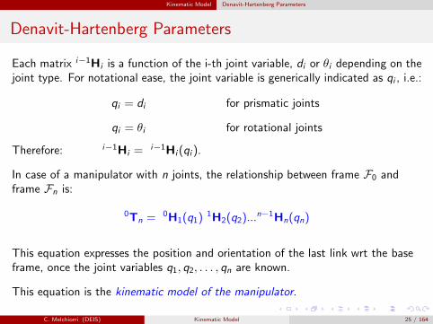
Each matrix i−1Hi is a function of the i-th joint variable, di or θi depending on thejoint type. For notational ease, the joint variable is generically indicated as qi , i.e.:
qi = di for prismatic joints
qi = θi for rotational joints
Therefore: i−1Hi =i−1Hi (qi ).
In case of a manipulator with n joints, the relationship between frame F0 andframe Fn is:
0Tn = 0H1(q1)1H2(q2)...
n−1Hn(qn)
This equation expresses the position and orientation of the last link wrt the baseframe, once the joint variables q1, q2, . . . , qn are known.
This equation is the kinematic model of the manipulator.
C. Melchiorri (DEIS) Kinematic Model 25 / 164
Kinematic Model Denavit-Hartenberg Parameters
Reference Configuration of a Canonical Transformation
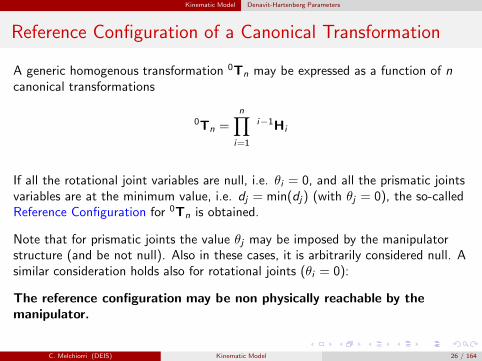
A generic homogenous transformation 0Tn may be expressed as a function of ncanonical transformations
0Tn =n∏
i=1
i−1Hi
If all the rotational joint variables are null, i.e. θi = 0, and all the prismatic jointsvariables are at the minimum value, i.e. dj = min(dj) (with θj = 0), the so-calledReference Configuration for 0Tn is obtained.
Note that for prismatic joints the value θj may be imposed by the manipulatorstructure (and be not null). Also in these cases, it is arbitrarily considered null. Asimilar consideration holds also for rotational joints (θi = 0):
The reference configuration may be non physically reachable by themanipulator.
C. Melchiorri (DEIS) Kinematic Model 26 / 164
Kinematic Model Denavit-Hartenberg Parameters
Kinematic Model
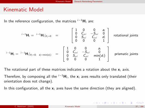
In the reference configuration, the matrices i−1Hi are:
i−1Hi =i−1Hi |θi=0 =
1 0 0 ai0 Cαi −Sαi 00 Sαi Cαi di0 0 0 1
rotational joints
i−1Hi =i−1Hi |θi=0; di=min(di ) =
1 0 0 ai0 Cαi −Sαi 00 Sαi Cαi min(di)0 0 0 1
prismatic joints
The rotational part of these matrices indicates a rotation about the xi axis.
Therefore, by composing all the i−1Hi , the xi axes results only translated (theirorientation does not change).
In this configuration, all the xi axes have the same direction (they are aligned).
C. Melchiorri (DEIS) Kinematic Model 27 / 164

Direct Kinematic Model Procedure for assigning frames
Kinematic Model of Robot ManipulatorsDirect Kinematic Model
Claudio Melchiorri
Dipartimento di Ingegneria dell’Energia Elettrica e dell’Informazione (DEI)
Universita di Bologna
email: [email protected]
C. Melchiorri (DEIS) Kinematic Model 28 / 164
Direct Kinematic Model Procedure for assigning frames
Kinematic Model
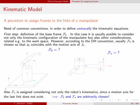
A procedure to assign frames to the links of a manipulator
Need of common conventions, in order to define univocally the kinematic equations.
First step: definition of the base frame F0 . In this case it is usually posible to considernot only the kinematic configuration of the manipulator but also other considerations,related e.g. to the work space. However, according to the DH convention, usually F0 ischosen so that z0 coincides with the motion axis of J1.
F0 = ?Fn = ?
Also Fn is assigned considering not only the robot’s kinematics, since a motion axis for
the last link does not exist. =⇒ F0 and Fn are arbitrarily chosen!
C. Melchiorri (DEIS) Kinematic Model 29 / 164
Direct Kinematic Model Procedure for assigning frames
Kinematic Model
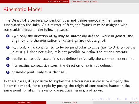
The Denavit-Hartenberg convention does not define univocally the framesassociated to the links. As a matter of fact, the frames may be assigned withsome arbitrariness in the following cases:
1 F0 : only the direction of z0 may be univocally defined, while in general theorigin o0 and the orientation of x0 and y0 are not assigned;
2 Fn : only xn is constrained to be perpendicular to zn−1 (i.e. to Jn). Since thejoint n + 1 does not exist, it is not possible to define the other elements;
3 parallel consecutive axes: it is not defined univocally the common normal line;
4 intersecting consecutive axes: the direction of xi is not defined;
5 prismatic joint: only zi is defined.
In these cases, it is possible to exploit the arbitrariness in order to simplify thekinematic model, for example by posing the origin of consecutive frames in thesame point, or aligning axes of consecutive frames, and so on.
C. Melchiorri (DEIS) Kinematic Model 30 / 164
Direct Kinematic Model Procedure for assigning frames
Procedure for assigning the frames
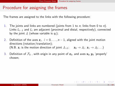
The frames are assigned to the links with the following procedure:
1. The joints and links are numbered (joints from 1 to n; links from 0 to n).Links Li−1 and Li are adjacent (proximal and distal, respectively), connectedby the joint Ji (whose variable is qi );
2. Definition of the axes zi , i = 0, . . . , n − 1, aligned with the joint motiondirections (rotation/translation);(N.B. zi is the motion direction of joint Ji+1: z0 → J1; z1 → J2; . . .)
3. Definition of F0 , with origin in any point of z0, and axes x0, y0 ‘properly’chosen;
C. Melchiorri (DEIS) Kinematic Model 31 / 164
Direct Kinematic Model Procedure for assigning frames
Procedure for assigning the frames
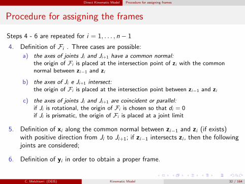
Steps 4 - 6 are repeated for i = 1, . . . , n− 1
4. Definition of Fi . Three cases are possible:
a) the axes of joints Ji and Ji+1 have a common normal:
the origin of Fi is placed at the intersection point of zi with the commonnormal between zi−1 and zi
b) the axes of Ji e Ji+1 intersect:
the origin of Fi is placed at the intersection point between zi−1 and zi
c) the axes of joints Ji and Ji+1 are coincident or parallel:
if Ji is rotational, the origin of Fi is chosen so that di = 0if Ji is prismatic, the origin of Fi is placed at a joint limit
5. Definition of xi along the common normal between zi−1 and zi (if exists)with positive direction from Ji to Ji+1; if zi−1 intersects zi , then the followingjoints are considered;
6. Definition of yi in order to obtain a proper frame.
C. Melchiorri (DEIS) Kinematic Model 32 / 164
Direct Kinematic Model Procedure for assigning frames
Procedure for assigning the frames
Finally:
7. Define on coincident with on−1;
8. Define xn perpendicular to zn−1;
9. If Jn is rotational, choose zn parallel to zn−1;If Jn is prismatic, it is possible to choose zn freely;
10. Define yn in order to obtain a proper frame.
Note that:
The position of on and its orientation zn are arbitrary
In this manner, the frame Fn is different wrt the frame of the end-effector tT(with axes n, s, a). Therefore, it is in general necessary to define a constanthomogeneous transform matrix to take into account this difference.
C. Melchiorri (DEIS) Kinematic Model 33 / 164
Direct Kinematic Model Procedure for assigning frames
Procedure for assigning the frames
Once the n frames Fi (i = 1, . . . , n) are defined, the corresponding 4n DHparameters di , ai , αi , θi can be easily determined, and therefore also thematrices i−1Hi can be computed. The kinematic model is then obtained.
Then:
a) Define the DH Parameters Table
b) Compute the homogeneous transformation matrices i−1Hi , i = 1, . . . , n
c) Compute the direct kinematic function
0Tn = 0H11H2 . . . n−1Hn
C. Melchiorri (DEIS) Kinematic Model 34 / 164
Direct Kinematic Model Examples
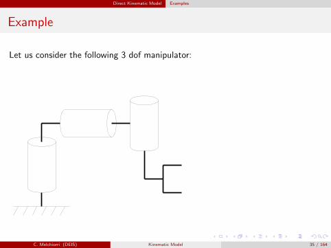
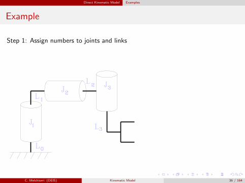
Example
Let us consider the following 3 dof manipulator:
C. Melchiorri (DEIS) Kinematic Model 35 / 164
Direct Kinematic Model Examples
Example
Step 1: Assign numbers to joints and links
C. Melchiorri (DEIS) Kinematic Model 36 / 164
Direct Kinematic Model Examples
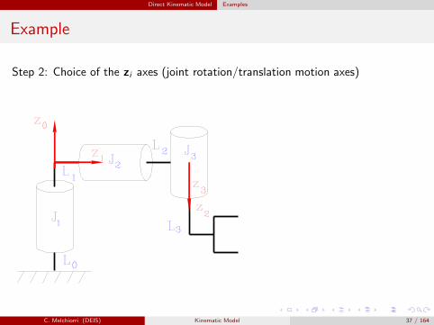
Example
Step 2: Choice of the zi axes (joint rotation/translation motion axes)
C. Melchiorri (DEIS) Kinematic Model 37 / 164
Direct Kinematic Model Examples
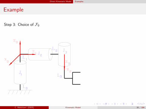
Example
Step 3: Choice of F0
C. Melchiorri (DEIS) Kinematic Model 38 / 164
Direct Kinematic Model Examples
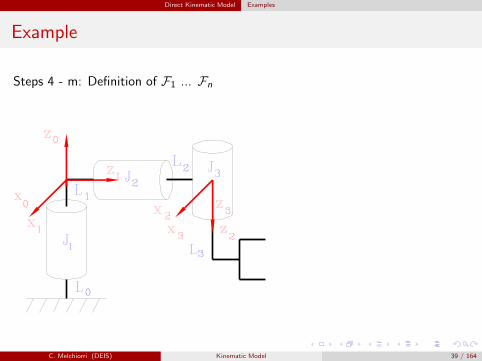
Example
Steps 4 - m: Definition of F1 ... Fn
C. Melchiorri (DEIS) Kinematic Model 39 / 164
Direct Kinematic Model Examples
Example
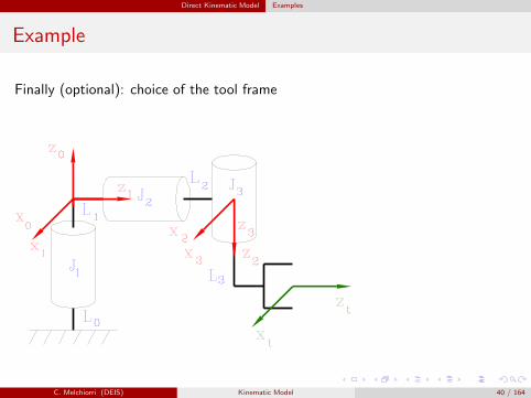
Finally (optional): choice of the tool frame
C. Melchiorri (DEIS) Kinematic Model 40 / 164
Direct Kinematic Model Examples
Example
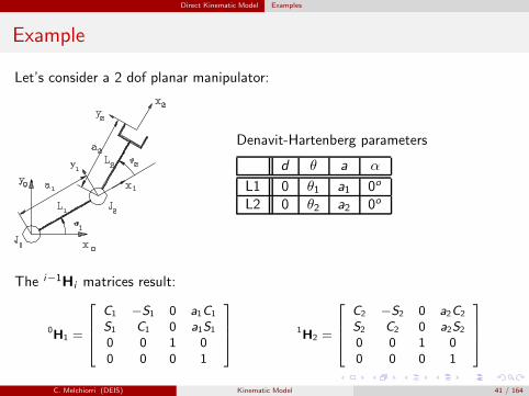
Let’s consider a 2 dof planar manipulator:
Denavit-Hartenberg parameters
d θ a α
L1 0 θ1 a1 0o
L2 0 θ2 a2 0o
The i−1Hi matrices result:
0H1 =
C1 −S1 0 a1C1
S1 C1 0 a1S1
0 0 1 00 0 0 1
1H2 =
C2 −S2 0 a2C2
S2 C2 0 a2S2
0 0 1 00 0 0 1
C. Melchiorri (DEIS) Kinematic Model 41 / 164
Direct Kinematic Model Examples
Example
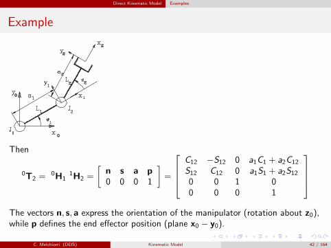
Then
0T2 =0H1
1H2 =
[
n s a p0 0 0 1
]
=
C12 −S12 0 a1C1 + a2C12
S12 C12 0 a1S1 + a2S120 0 1 00 0 0 1
The vectors n, s, a express the orientation of the manipulator (rotation about z0),while p defines the end effector position (plane x0 − y0).
C. Melchiorri (DEIS) Kinematic Model 42 / 164
Direct Kinematic Model Examples
Example
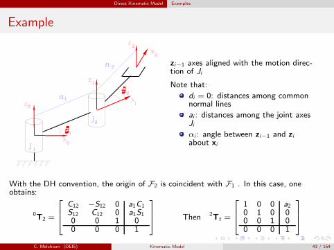
zi−1 axes aligned with the motion direc-tion of Ji
Note that:
di = 0: distances among commonnormal lines
ai : distances among the joint axesJi
αi : angle between zi−1 and ziabout xi
With the DH convention, the origin of F2 is coincident with F1 . In this case, oneobtains:
0T2 =
C12 −S12 0 a1C1
S12 C12 0 a1S1
0 0 1 00 0 0 1
Then 2Tt =
1 0 0 a20 1 0 00 0 1 00 0 0 1
C. Melchiorri (DEIS) Kinematic Model 43 / 164
Direct Kinematic Model Examples
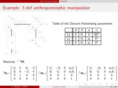
Example: 3 dof anthropomorphic manipulator
Table of the Denavit-Hartenberg parameters
d θ a α
L1 0 θ1 0 90o
L2 0 θ2 a2 0o
L3 0 θ3 a3 0o
Matrices i−1Hi
0H1=
C1 0 S1 0S1 0 −C1 00 1 0 00 0 0 1
,1 H2=
C2 −S2 0 a2C2
S2 C2 0 a2S2
0 0 1 00 0 0 1
,2 H3=
C3 −S3 0 a3C3
S3 C3 0 a3S3
0 0 1 00 0 0 1
C. Melchiorri (DEIS) Kinematic Model 44 / 164
Direct Kinematic Model Examples
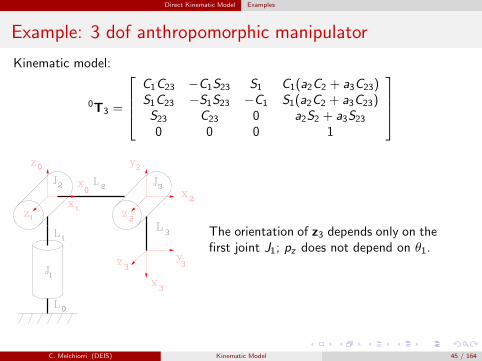
Example: 3 dof anthropomorphic manipulator
Kinematic model:
0T3 =
C1C23 −C1S23 S1 C1(a2C2 + a3C23)S1C23 −S1S23 −C1 S1(a2C2 + a3C23)S23 C23 0 a2S2 + a3S230 0 0 1
The orientation of z3 depends only on thefirst joint J1; pz does not depend on θ1.
C. Melchiorri (DEIS) Kinematic Model 45 / 164
Direct Kinematic Model Examples
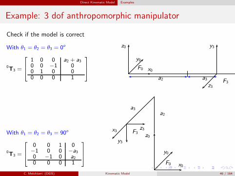
Example: 3 dof anthropomorphic manipulator
Check if the model is correct
With θ1 = θ2 = θ3 = 0o
0T3 =
1 0 0 a2 + a30 0 −1 00 1 0 00 0 0 1
x0
z0
y0
F0
a2 a3
y3
z3F3
With θ1 = θ2 = θ3 = 90o
0T3 =
0 0 1 0−1 0 0 −a30 −1 0 a20 0 0 1
x0
z0
y0
F0
a2a3
z3
y3
x3 F3
C. Melchiorri (DEIS) Kinematic Model 46 / 164
Direct Kinematic Model Examples
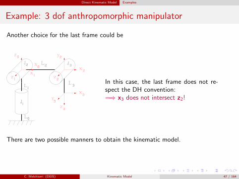
Example: 3 dof anthropomorphic manipulator
Another choice for the last frame could be
In this case, the last frame does not re-spect the DH convention:=⇒ x3 does not intersect z2!
There are two possible manners to obtain the kinematic model.
C. Melchiorri (DEIS) Kinematic Model 47 / 164
Direct Kinematic Model Examples
Example: 3 dof anthropomorphic manipulator
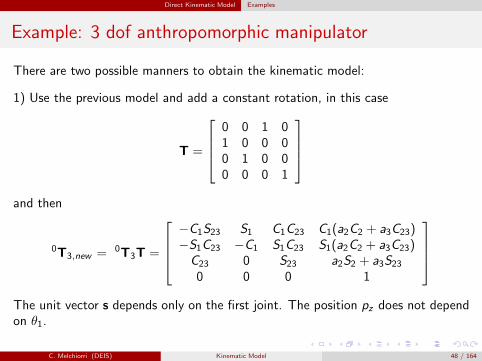
There are two possible manners to obtain the kinematic model:
1) Use the previous model and add a constant rotation, in this case
T =
0 0 1 01 0 0 00 1 0 00 0 0 1
and then
0T3,new = 0T3T =
−C1S23 S1 C1C23 C1(a2C2 + a3C23)−S1C23 −C1 S1C23 S1(a2C2 + a3C23)C23 0 S23 a2S2 + a3S230 0 0 1
The unit vector s depends only on the first joint. The position pz does not dependon θ1.
C. Melchiorri (DEIS) Kinematic Model 48 / 164
Direct Kinematic Model Examples
Example: 3 dof anthropomorphic manipulator
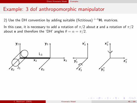
2) Use the DH convention by adding suitable (fictitious) i−1Hi matrices.
In this case, it is necessary to add a rotation of π/2 about z and a rotation of π/2about x and therefore the ‘DH’ angles θ = α = π/2.
x2
y2
z2J3
L3
x3
y3
z3
y′3
x′3
z′3
z′′3
x′′3
y′′3
C. Melchiorri (DEIS) Kinematic Model 49 / 164
Direct Kinematic Model Examples
Example: 3 dof anthropomorphic manipulator
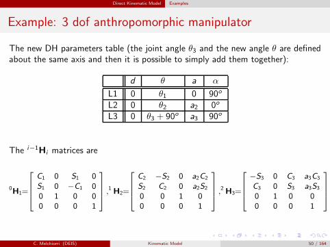
The new DH parameters table (the joint angle θ3 and the new angle θ are definedabout the same axis and then it is possible to simply add them together):
d θ a α
L1 0 θ1 0 90o
L2 0 θ2 a2 0o
L3 0 θ3 + 90o a3 90o
The i−1Hi matrices are
0H1=
C1 0 S1 0S1 0 −C1 00 1 0 00 0 0 1
,1 H2=
C2 −S2 0 a2C2
S2 C2 0 a2S2
0 0 1 00 0 0 1
,2 H3=
−S3 0 C3 a3C3
C3 0 S3 a3S3
0 1 0 00 0 0 1
C. Melchiorri (DEIS) Kinematic Model 50 / 164
Direct Kinematic Model Examples
Example: 3 dof anthropomorphic manipulator
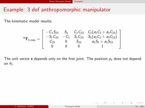
The kinematic model results:
0T3,new =
−C1S23 S1 C1C23 C1(a2C2 + a3C23)−S1C23 −C1 S1C23 S1(a2C2 + a3C23)C23 0 S23 a2S2 + a3S230 0 0 1
The unit vector s depends only on the first joint. The position pz does not dependon θ1.
C. Melchiorri (DEIS) Kinematic Model 51 / 164
Direct Kinematic Model Examples
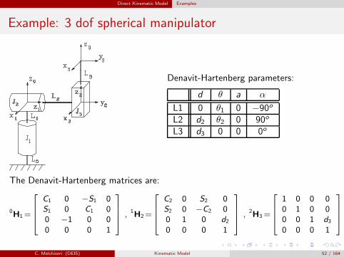
Example: 3 dof spherical manipulator
Denavit-Hartenberg parameters:
d θ a α
L1 0 θ1 0 −90o
L2 d2 θ2 0 90o
L3 d3 0 0 0o
The Denavit-Hartenberg matrices are:
0H1=
C1 0 −S1 0S1 0 C1 00 −1 0 00 0 0 1
, 1H2=
C2 0 S2 0S2 0 −C2 00 1 0 d20 0 0 1
, 2H3=
1 0 0 00 1 0 00 0 1 d30 0 0 1
C. Melchiorri (DEIS) Kinematic Model 52 / 164
Direct Kinematic Model Examples
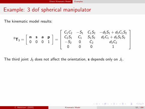
Example: 3 dof spherical manipulator
The kinematic model results:
0T3 =
[
n s a p0 0 0 1
]
=
C1C2 −S1 C1S2 −d2S1 + d3C1S2C2S1 C1 S1S2 d2C1 + d3S1S2−S2 0 C2 d3C2
0 0 0 1
The third joint J3 does not affect the orientation, s depends only on J1.
C. Melchiorri (DEIS) Kinematic Model 53 / 164
Direct Kinematic Model Examples
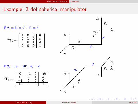
Example: 3 dof spherical manipulator
If θ1 = θ2 = 0o , d3 = d
0T3 =
1 0 0 00 1 0 d20 0 1 d0 0 0 1
y0
z0
x0
F0d2
d
y3
z3
x3
F3
If θ1 = θ2 = 90o , d3 = d
0T3 =
0 −1 0 −d20 0 1 d−1 0 0 00 0 0 1
y0
z0
x0
F0
−d2
d
z3
x3
y3
F3
C. Melchiorri (DEIS) Kinematic Model 54 / 164
Direct Kinematic Model Examples
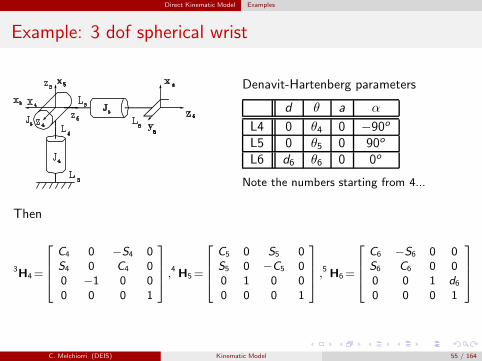
Example: 3 dof spherical wrist
Denavit-Hartenberg parameters
d θ a α
L4 0 θ4 0 −90o
L5 0 θ5 0 90o
L6 d6 θ6 0 0o
Note the numbers starting from 4...
Then
3H4=
C4 0 −S4 0S4 0 C4 00 −1 0 00 0 0 1
,4 H5=
C5 0 S5 0S5 0 −C5 00 1 0 00 0 0 1
,5 H6=
C6 −S6 0 0S6 C6 0 00 0 1 d60 0 0 1
C. Melchiorri (DEIS) Kinematic Model 55 / 164
Direct Kinematic Model Examples
Example: 3 dof spherical wrist
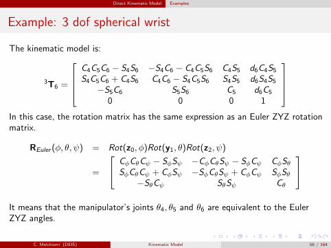
The kinematic model is:
3T6 =
C4C5C6 − S4S6 −S4C6 − C4C5S6 C4S5 d6C4S5S4C5C6 + C4S6 C4C6 − S4C5S6 S4S5 d6S4S5
−S5C6 S5S6 C5 d6C5
0 0 0 1
In this case, the rotation matrix has the same expression as an Euler ZYZ rotationmatrix.
REuler (φ, θ, ψ) = Rot(z0, φ)Rot(y1, θ)Rot(z2, ψ)
=
CφCθCψ − SφSψ −CφCθSψ − SφCψ CφSθSφCθCψ + CφSψ −SφCθSψ + CφCψ SφSθ
−SθCψ SθSψ Cθ
It means that the manipulator’s joints θ4, θ5 and θ6 are equivalent to the EulerZYZ angles.
C. Melchiorri (DEIS) Kinematic Model 56 / 164
Direct Kinematic Model Examples
Example: 3 dof spherical wrist
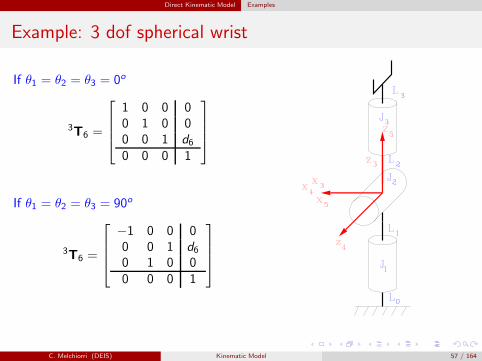
If θ1 = θ2 = θ3 = 0o
3T6 =
1 0 0 00 1 0 00 0 1 d60 0 0 1
If θ1 = θ2 = θ3 = 90o
3T6 =
−1 0 0 00 0 1 d60 1 0 00 0 0 1
C. Melchiorri (DEIS) Kinematic Model 57 / 164
Direct Kinematic Model Examples
Example: Stanford manipulator
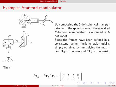
By composing the 3 dof spherical manipu-lator with the spherical wrist, the so-called“Stanford manipulator” is obtained, a 6dof robot.Since the frames have been defined in aconsistent manner, the kinematic model issimply obtained by multiplying the matri-ces 0T3 of the arm and 3T6 of the wrist.
Then
0T6 =0T3
3T6 =
[
n s a p0 0 0 1
]
C. Melchiorri (DEIS) Kinematic Model 58 / 164
Direct Kinematic Model Examples
Example: Stanford manipulator
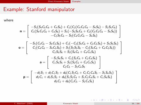
where
n =
−S1(S4C5C6 + C4S6) + C1(C2(C4C5C6 − S4S6)− S2S5C6)C1(S4C5C6 + C4S6) + S1(−S2S5C6 + C2(C4C5C6 − S4S6))
−C2S5C6 − S2(C4C5C6 − S4S6)
o =
−S1(C4C6 − S4C5S6) + C1(−C2(S4C6 + C4C5S6) + S2S5S6)C1(C4C6 − S4C5S6) + S1(S2S5S6 − C2(S4C6 + C4C5S6))
C2S5S6 + S2(S4C6 + C4C5S6)
a =
−S1S4S5 + C1(S2C5 + C2C4S5)C1S4S5 + S1(S2C5 + C2C4S5)
C2C5 − S2C4S5
p =
−d2S1 + d3C1S2 + d6(C1S2C5 + C1C2C4S5 − S1S4S5)d2C1 + d3S1S2 + d6(S1S2C5 + S1C2C4S5 + C1S4S5)
d3C2 + d6(C2C5 − S2C4S5)
C. Melchiorri (DEIS) Kinematic Model 59 / 164
Direct Kinematic Model Examples
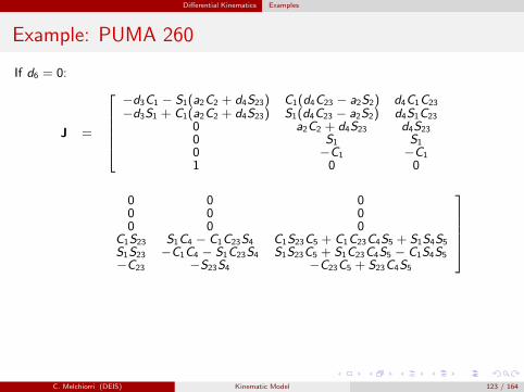
Example: PUMA 260
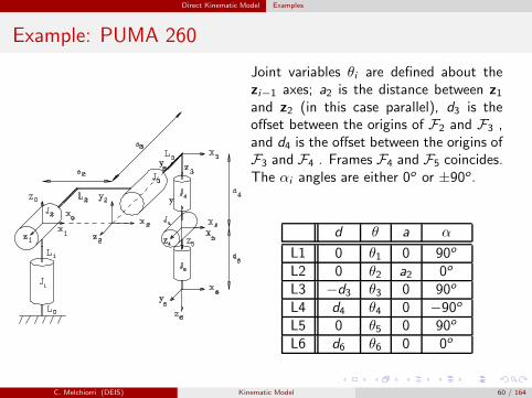
Joint variables θi are defined about thezi−1 axes; a2 is the distance between z1and z2 (in this case parallel), d3 is theoffset between the origins of F2 and F3 ,and d4 is the offset between the origins ofF3 and F4 . Frames F4 and F5 coincides.The αi angles are either 0o or ±90o.
d θ a α
L1 0 θ1 0 90o
L2 0 θ2 a2 0o
L3 −d3 θ3 0 90o
L4 d4 θ4 0 −90o
L5 0 θ5 0 90o
L6 d6 θ6 0 0o
C. Melchiorri (DEIS) Kinematic Model 60 / 164
Direct Kinematic Model Examples
Example: PUMA 260
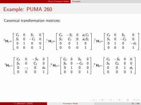
Canonical transformation matrices:
0H1=
C1 0 S1 0S1 0 −C1 00 1 0 00 0 0 1
,1 H2=
C2 −S2 0 a2C2
S2 C2 0 a2S2
0 0 1 00 0 0 1
,2 H3=
C3 0 S3 0S3 0 −C3 00 1 0 −d30 0 0 1
3H4=
C4 0 −S4 0S4 0 C4 00 −1 0 d40 0 0 1
,4 H5=
C5 0 S5 0S5 0 −C5 00 1 0 00 0 0 1
,5 H6=
C6 −S6 0 0S6 C6 0 00 0 1 d60 0 0 1
C. Melchiorri (DEIS) Kinematic Model 61 / 164
Direct Kinematic Model Examples
Example: PUMA 260
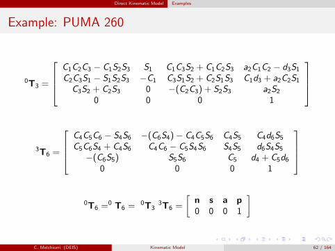
0T3 =
C1C2C3 − C1S2S3 S1 C1C3S2 + C1C2S3 a2C1C2 − d3S1C2C3S1 − S1S2S3 −C1 C3S1S2 + C2S1S3 C1d3 + a2C2S1C3S2 + C2S3 0 −(C2C3) + S2S3 a2S2
0 0 0 1
3T6 =
C4C5C6 − S4S6 −(C6S4)− C4C5S6 C4S5 C4d6S5C5C6S4 + C4S6 C4C6 − C5S4S6 S4S5 d6S4S5
−(C6S5) S5S6 C5 d4 + C5d60 0 0 1
0T6 =0 T6 =
0T33T6 =
[
n s a p0 0 0 1
]
C. Melchiorri (DEIS) Kinematic Model 62 / 164
Direct Kinematic Model Examples
Example: PUMA 260
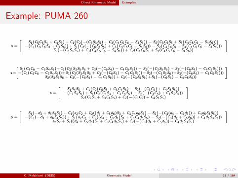
n =
[
S1(C5C6S4 + C4S6) + C1(C2(−(C6S3S5) + C3(C4C5C6 − S4S6)) − S2(C3C6S5 + S3(C4C5C6 − S4S6)))−(C1(C5C6S4 + C4S6)) + S1(C2(−(C6S3S5) + C3(C4C5C6 − S4S6)) − S2(C3C6S5 + S3(C4C5C6 − S4S6)))
S2(−(C6S3S5) + C3(C4C5C6 − S4S6)) + C2(C3C6S5 + S3(C4C5C6 − S4S6))
]
s=
[
S1(C4C6 − C5S4S6)+C1(C2(S3S5S6 + C3(−(C6S4) − C4C5S6)) − S2(−(C3S5S6) + S3(−(C6S4) − C4C5S6)))−(C1(C4C6 − C5S4S6))+S1(C2(S3S5S6 + C3(−(C6S4) − C4C5S6))−S2(−(C3S5S6)+S3(−(C6S4) − C4C5S6)))
S2(S3S5S6 + C3(−(C6S4) − C4C5S6)) + C2(−(C3S5S6)+S3(−(C6S4) − C4C5S6))
]
a =
[
S1S4S5 + C1(C2(C5S3 + C3C4S5) − S2(−(C3C5) + C4S3S5))−(C1S4S5) + S1(C2(C5S3 + C3C4S5) − S2(−(C3C5) + C4S3S5))
S2(C5S3 + C3C4S5) + C2(−(C3C5) + C4S3S5)
]
p =
[
S1(−d3 + d6S4S5) + C1(a2C2 + C2((d4 + C5d6)S3 + C3C4d6S5) − S2(−(C3(d4 + C5d6)) + C4d6S3S5))−(C1(−d3 + d6S4S5)) + S1(a2C2 + C2((d4 + C5d6)S3 + C3C4d6S5) − S2(−(C3(d4 + C5d6)) + C4d6S3S5))
a2S2 + S2((d4 + C5d6)S3 + C3C4d6S5) + C2(−(C3(d4 + C5d6)) + C4d6S3S5)
]
C. Melchiorri (DEIS) Kinematic Model 63 / 164
Direct Kinematic Model Examples
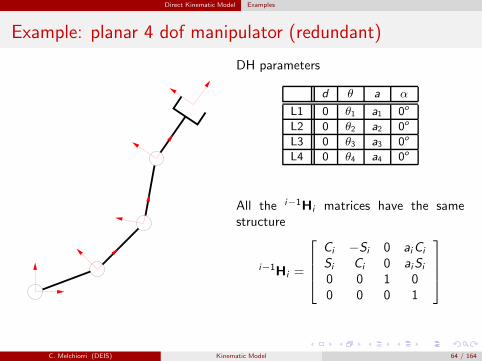
Example: planar 4 dof manipulator (redundant)
DH parameters
d θ a α
L1 0 θ1 a1 0o
L2 0 θ2 a2 0o
L3 0 θ3 a3 0o
L4 0 θ4 a4 0o
All the i−1Hi matrices have the samestructure
i−1Hi =
Ci −Si 0 aiCi
Si Ci 0 aiSi0 0 1 00 0 0 1
C. Melchiorri (DEIS) Kinematic Model 64 / 164
Direct Kinematic Model Examples
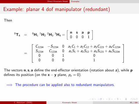
Example: planar 4 dof manipulator (redundant)
Then
0T4 = 0H11H2
2H33H4 =
[
n s a p0 0 0 1
]
=
C1234 −S1234 0 a1C1 + a2C12 + a3C123 + a4C1234
S1234 C1234 0 a1S1 + a2S12 + a3S123 + a4S12340 0 1 00 0 0 1
The vectors n, s, a define the end-effector orientation (rotation about z), while pdefines its position (on the x− y plane, pz = 0).
=⇒ The procedure can be applied also to redundant manipulators.
C. Melchiorri (DEIS) Kinematic Model 65 / 164

Inverse Kinematic Model
Kinematic Model of Robot ManipulatorsInverse Kinematic Model
Claudio Melchiorri
Dipartimento di Ingegneria dell’Energia Elettrica e dell’Informazione (DEI)
Universita di Bologna
email: [email protected]
C. Melchiorri (DEIS) Kinematic Model 66 / 164
Inverse Kinematic Model Introduction
Inverse Kinematic Model
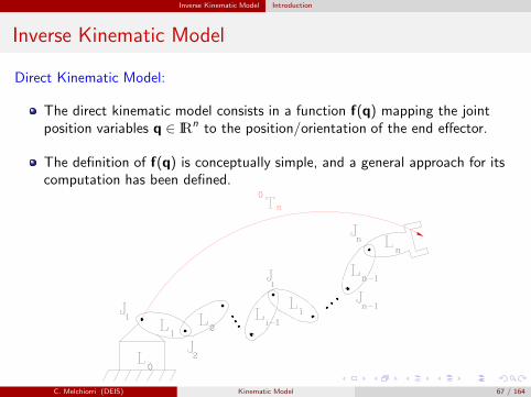
Direct Kinematic Model:
The direct kinematic model consists in a function f(q) mapping the jointposition variables q ∈ IR
n to the position/orientation of the end effector.
The definition of f(q) is conceptually simple, and a general approach for itscomputation has been defined.
C. Melchiorri (DEIS) Kinematic Model 67 / 164
Inverse Kinematic Model Introduction
Inverse Kinematic Model
Inverse Kinematic Model:
The inverse kinematics consists in finding a function g(x) mapping theposition/orientation of the end-effector to the corresponding joint variables q:the problem is not simple!
A general approach for the solution of this problem does not exist
On the other hand, for the most common kinematic structures, a scheme forobtaining the solution has been found. Unfortunately
The solution is not unique. In general we have:No solution (e.g. starting with a position x not in the workspace);A finite set of solutions (one or more);Infinite solutions.
We seek for closed form solutions, and not based on numerical techniques:
The analytic solution is more efficient from the computational point of view;If the solutions are known analytically, it is possible to select one of them onthe basis of proper criteria.
C. Melchiorri (DEIS) Kinematic Model 68 / 164
Inverse Kinematic Model Introduction
Inverse Kinematic Model
In order to obtain a closed form solution to the inverse kinematic problem, twoapproaches are possible:
An algebraic approach, i.e. elaborations of the kinematic equations until asuitable set of (simple) equations is obtained for the solution
A geometric approach based, when possible, on geometrical considerations,dependent on the kinematic structure of the manipulator and that may helpin the solution.
C. Melchiorri (DEIS) Kinematic Model 69 / 164
Inverse Kinematic Model Algebraic Approach
Algebraic Approach
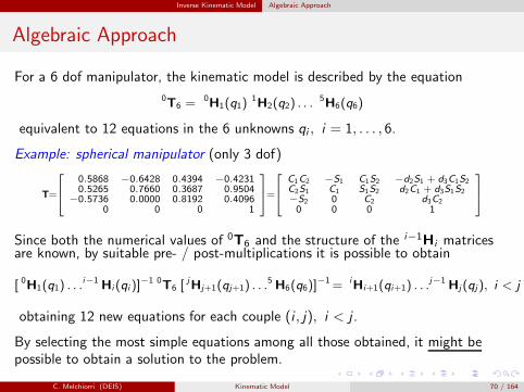
For a 6 dof manipulator, the kinematic model is described by the equation
0T6 =0H1(q1)
1H2(q2) . . .5H6(q6)
equivalent to 12 equations in the 6 unknowns qi , i = 1, . . . , 6.
Example: spherical manipulator (only 3 dof)
T=
0.5868 −0.6428 0.4394 −0.42310.5265 0.7660 0.3687 0.9504
−0.5736 0.0000 0.8192 0.40960 0 0 1
=
C1C2 −S1 C1S2 −d2S1 + d3C1S2C2S1 C1 S1S2 d2C1 + d3S1S2−S2 0 C2 d3C20 0 0 1
Since both the numerical values of 0T6 and the structure of the i−1Hi matricesare known, by suitable pre- / post-multiplications it is possible to obtain
[ 0H1(q1) . . .i−1 Hi (qi )]
−1 0T6 [jHj+1(qj+1) . . .
5 H6(q6)]−1= iHi+1(qi+1) . . .
j−1 Hj (qj ), i < j
obtaining 12 new equations for each couple (i , j), i < j .
By selecting the most simple equations among all those obtained, it might bepossible to obtain a solution to the problem.
C. Melchiorri (DEIS) Kinematic Model 70 / 164
Inverse Kinematic Model Geometric Approach
Geometric Approach
General considerations that may help in finding solutions with algebraic techniquesdo not exist, being these strictly related to the mathematical expression of thedirect kinematic model. On the other hand, it is often possible to exploitconsiderations related to the geometrical structure of the manipulator.
PIEPER APPROACH
Many industrial manipulators have a kinematically decoupled structure, forwhich it is possible to decompose the problem in two (simpler) sub-problems:
1 Inverse kinematics for the position (x , y , z) → q1, q2, q3
2 Inverse kinematics for the orientation R → q4, q5, q6.
C. Melchiorri (DEIS) Kinematic Model 71 / 164
Inverse Kinematic Model Geometric Approach
Geometric Approach
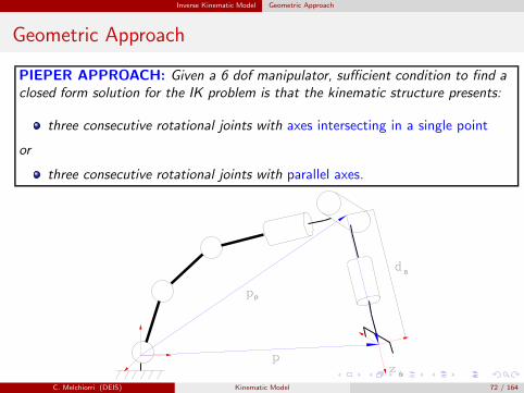
PIEPER APPROACH: Given a 6 dof manipulator, sufficient condition to find aclosed form solution for the IK problem is that the kinematic structure presents:
three consecutive rotational joints with axes intersecting in a single point
or
three consecutive rotational joints with parallel axes.
C. Melchiorri (DEIS) Kinematic Model 72 / 164
Inverse Kinematic Model Geometric Approach
Geometric Approach
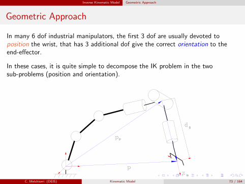
In many 6 dof industrial manipulators, the first 3 dof are usually devoted toposition the wrist, that has 3 additional dof give the correct orientation to theend-effector.
In these cases, it is quite simple to decompose the IK problem in the twosub-problems (position and orientation).
C. Melchiorri (DEIS) Kinematic Model 73 / 164
Inverse Kinematic Model Geometric Approach
Geometric Approach
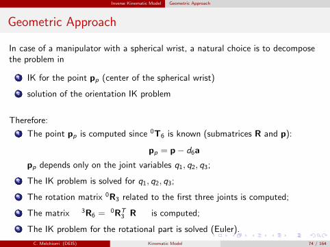
In case of a manipulator with a spherical wrist, a natural choice is to decomposethe problem in
1 IK for the point pp (center of the spherical wrist)
2 solution of the orientation IK problem
Therefore:
1 The point pp is computed since 0T6 is known (submatrices R and p):
pp = p− d6a
pp depends only on the joint variables q1, q2, q3;
2 The IK problem is solved for q1, q2, q3;
3 The rotation matrix 0R3 related to the first three joints is computed;
4 The matrix 3R6 =0RT
3 R is computed;
5 The IK problem for the rotational part is solved (Euler).
C. Melchiorri (DEIS) Kinematic Model 74 / 164
Inverse Kinematic Model Examples
Solution of the spherical manipulator
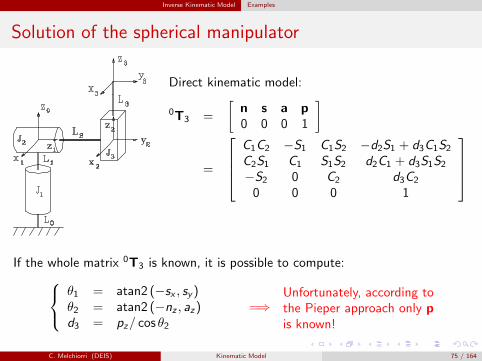
Direct kinematic model:
0T3 =
[
n s a p0 0 0 1
]
=
C1C2 −S1 C1S2 −d2S1 + d3C1S2C2S1 C1 S1S2 d2C1 + d3S1S2−S2 0 C2 d3C2
0 0 0 1
If the whole matrix 0T3 is known, it is possible to compute:
θ1 = atan2 (−sx , sy)θ2 = atan2 (−nz , az)d3 = pz/ cos θ2
=⇒Unfortunately, according tothe Pieper approach only pis known!
C. Melchiorri (DEIS) Kinematic Model 75 / 164
Inverse Kinematic Model Examples
Solution of the spherical manipulator
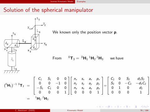
We known only the position vector p.
From 0T3 =0H1
1H22H3 we have
(0H1)−1 0T3 =
C1 S1 0 00 0 −1 0
−S1 C1 0 00 0 0 1
nx sx ax pxny sy ay pynz sz az pz0 0 0 1
=
C2 0 S2 d3S2
S2 0 −C2 −d3C2
0 1 0 d20 0 0 1
= 1H22H3
C. Melchiorri (DEIS) Kinematic Model 76 / 164
Inverse Kinematic Model Examples
Solution of the spherical manipulator
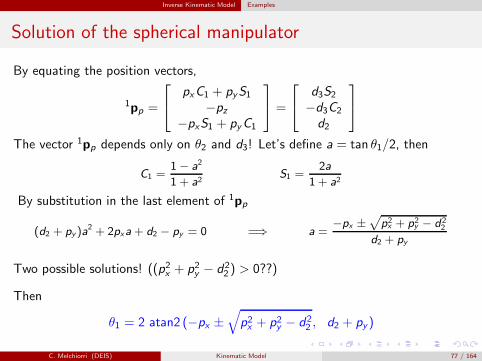
By equating the position vectors,
1pp =
pxC1 + pyS1−pz
−pxS1 + pyC1
=
d3S2−d3C2
d2
The vector 1pp depends only on θ2 and d3! Let’s define a = tan θ1/2, then
C1 =1− a2
1 + a2S1 =
2a
1 + a2
By substitution in the last element of 1pp
(d2 + py )a2 + 2pxa + d2 − py = 0 =⇒ a =
−px ±√
p2x + p2
y − d22
d2 + py
Two possible solutions! ((p2x + p2y − d22 ) > 0??)
Then
θ1 = 2 atan2 (−px ±√
p2x + p2y − d22 , d2 + py )
C. Melchiorri (DEIS) Kinematic Model 77 / 164
Inverse Kinematic Model Examples
Solution of the spherical manipulator
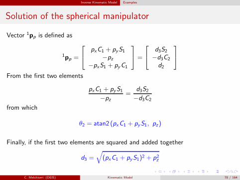
Vector 1pp is defined as
1pp =
pxC1 + pyS1−pz
−pxS1 + pyC1
=
d3S2−d3C2
d2
From the first two elements
pxC1 + pyS1−pz
=d3S2−d3C2
from which
θ2 = atan2 (pxC1 + pyS1, pz)
Finally, if the first two elements are squared and added together
d3 =√
(pxC1 + pyS1)2 + p2z
C. Melchiorri (DEIS) Kinematic Model 78 / 164
Inverse Kinematic Model Examples
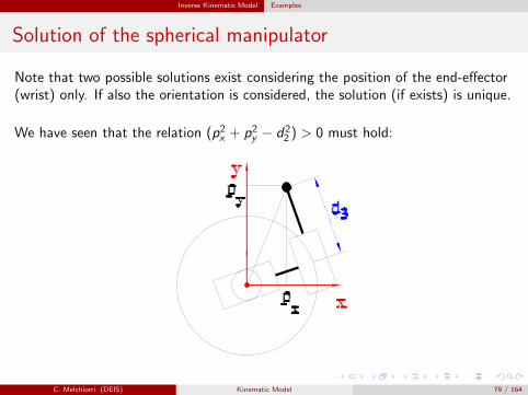
Solution of the spherical manipulator
Note that two possible solutions exist considering the position of the end-effector(wrist) only. If also the orientation is considered, the solution (if exists) is unique.
We have seen that the relation (p2x + p2y − d22 ) > 0 must hold:
C. Melchiorri (DEIS) Kinematic Model 79 / 164

Inverse Kinematic Model Examples
Solution of the spherical manipulator
Numerical example: Given a spherical manipulator with d2 = 0.8 m in the pose
θ1 = 20o , θ2 = 30o, d3 = 0.5 m
we have
0T3 =
0.8138 −0.342 0.4698 −0.03870.2962 0.9397 0.171 0.8373−0.5 0 0.866 0.433
0 0 0 1
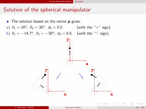
• The solution based on the whole matrix 0T3 is: θ1 = 20o , θ2 = 30o , d3 = 0.5.
• The solution based on the vector p gives:
a) θ1 = 20o , θ2 = 30o , d3 = 0.5 (with the “+” sign).
b) θ1 = −14.7o, θ2 = −30o , d3 = 0.5 (with the “-” sign).
C. Melchiorri (DEIS) Kinematic Model 80 / 164
Inverse Kinematic Model Examples
Solution of the spherical manipulator
• The solution based on the vector p gives:
a) θ1 = 20o , θ2 = 30o , d3 = 0.5 (with the “+” sign).
b) θ1 = −14.7o, θ2 = −30o , d3 = 0.5 (with the “-” sign).
C. Melchiorri (DEIS) Kinematic Model 81 / 164
Inverse Kinematic Model Examples
Solution of the 3 dof anthropomorphic manipulator
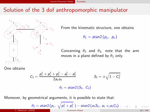
From the kinematic structure, one obtains
θ1 = atan2 (py , px)
Concerning θ2 and θ3, note that the armmoves in a plane defined by θ1 only.
One obtains
C3 =p2x + p2
y + p2z − a22 − a23
2a2a3S3 = ±
√
1− C 23
θ3 = atan2 (S3, C3)
Moreover, by geometrical arguments, it is possible to state that:
θ2 = atan2 (pz ,√
p2x + p2
y )− atan2 (a3S3, a2 + a3C3)C. Melchiorri (DEIS) Kinematic Model 82 / 164
Inverse Kinematic Model Examples
Solution of the 3 dof anthropomorphic manipulator
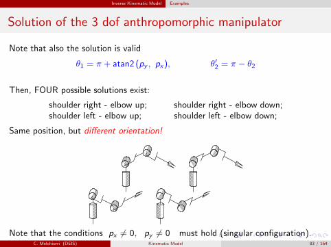
Note that also the solution is valid
θ1 = π + atan2 (py , px), θ′2 = π − θ2
Then, FOUR possible solutions exist:
shoulder right - elbow up; shoulder right - elbow down;shoulder left - elbow up; shoulder left - elbow down;
Same position, but different orientation!
Note that the conditions px 6= 0, py 6= 0 must hold (singular configuration).C. Melchiorri (DEIS) Kinematic Model 83 / 164
Inverse Kinematic Model Examples
Solution of the spherical wrist
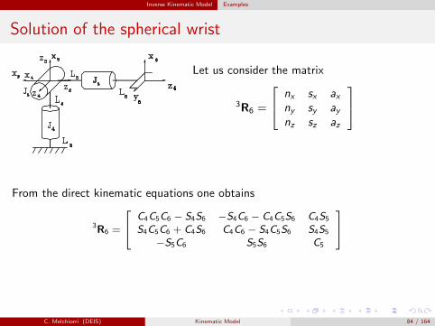
Let us consider the matrix
3R6 =
nx sx axny sy aynz sz az
From the direct kinematic equations one obtains
3R6 =
C4C5C6 − S4S6 −S4C6 − C4C5S6 C4S5
S4C5C6 + C4S6 C4C6 − S4C5S6 S4S5
−S5C6 S5S6 C5
C. Melchiorri (DEIS) Kinematic Model 84 / 164
Inverse Kinematic Model Examples
Solution of the spherical wrist
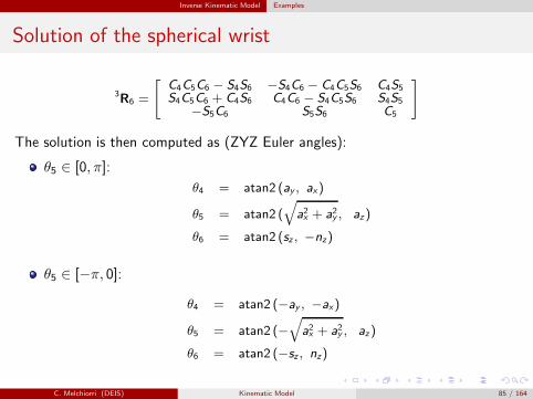
3R6 =
[
C4C5C6 − S4S6 −S4C6 − C4C5S6 C4S5
S4C5C6 + C4S6 C4C6 − S4C5S6 S4S5
−S5C6 S5S6 C5
]
The solution is then computed as (ZYZ Euler angles):
θ5 ∈ [0, π]:
θ4 = atan2 (ay , ax)
θ5 = atan2 (√
a2x + a2y , az )
θ6 = atan2 (sz , −nz)
θ5 ∈ [−π, 0]:
θ4 = atan2 (−ay , −ax)
θ5 = atan2 (−√
a2x + a2y , az )
θ6 = atan2 (−sz , nz)
C. Melchiorri (DEIS) Kinematic Model 85 / 164
Inverse Kinematic Model Examples
Solution of the spherical wrist
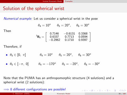
Numerical example: Let us consider a spherical wrist in the pose
θ4 = 10o θ5 = 20o, θ6 = 30o
Then3R6 =
[
0.7146 −0.6131 0.33680.6337 0.7713 0.0594−0.2962 0.1710 0.9397
]
Therefore, if
• θ5 ∈ [0, π] θ4 = 10o θ5 = 20o , θ6 = 30o
• θ5 ∈ [−π, 0] θ4 = −170o θ5 = −20o, θ6 = −30o
Note that the PUMA has an anthropomorphic structure (4 solutions) and aspherical wrist (2 solutions):
=⇒ 8 different configurations are possible!C. Melchiorri (DEIS) Kinematic Model 86 / 164

Differential Kinematics
Kinematic Model of Robot ManipulatorsDifferential Kinematics
Claudio Melchiorri
Dipartimento di Ingegneria dell’Energia Elettrica e dell’Informazione (DEI)
Universita di Bologna
email: [email protected]
C. Melchiorri (DEIS) Kinematic Model 87 / 164
Differential Kinematics Introduction
Differential Kinematics: the Jacobian matrix
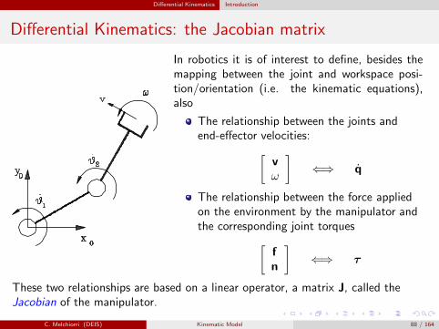
In robotics it is of interest to define, besides themapping between the joint and workspace posi-tion/orientation (i.e. the kinematic equations),also
The relationship between the joints andend-effector velocities:
[
vω
]
⇐⇒ q
The relationship between the force appliedon the environment by the manipulator andthe corresponding joint torques
[
fn
]
⇐⇒ τ
These two relationships are based on a linear operator, a matrix J, called theJacobian of the manipulator.
C. Melchiorri (DEIS) Kinematic Model 88 / 164
Differential Kinematics Introduction
The Jacobian matrix
In robotics, the Jacobian is used for several purposes:
To define the relationship between joint and workspace velocities
To define the relationship between forces/torques between the spaces
To study the singular configurations
To define numerical procedures for the solution of the IK problem
To study the manipulability properties.
C. Melchiorri (DEIS) Kinematic Model 89 / 164
Differential Kinematics The Jacobian Matrix
Velocity domain
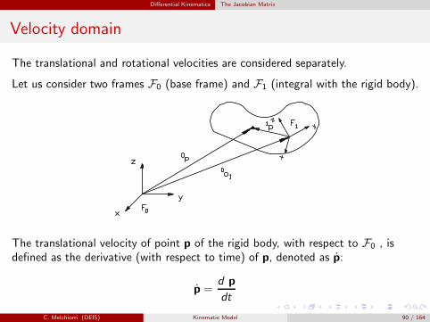
The translational and rotational velocities are considered separately.
Let us consider two frames F0 (base frame) and F1 (integral with the rigid body).
The translational velocity of point p of the rigid body, with respect to F0 , isdefined as the derivative (with respect to time) of p, denoted as p:
p =d p
dt
C. Melchiorri (DEIS) Kinematic Model 90 / 164
Differential Kinematics The Jacobian Matrix
Velocity domain
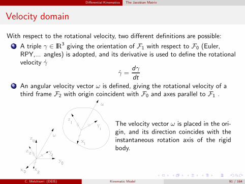
With respect to the rotational velocity, two different definitions are possible:
1 A triple γ ∈ IR3 giving the orientation of F1 with respect to F0 (Euler,
RPY,... angles) is adopted, and its derivative is used to define the rotationalvelocity γ
γ =dγ
dt2 An angular velocity vector ω is defined, giving the rotational velocity of a
third frame F2 with origin coincident with F0 and axes parallel to F1 .
The velocity vector ω is placed in the ori-gin, and its direction coincides with theinstantaneous rotation axis of the rigidbody.
C. Melchiorri (DEIS) Kinematic Model 91 / 164
Differential Kinematics The Jacobian Matrix
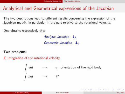
Analytical and Geometrical expressions of the Jacobian
The two descriptions lead to different results concerning the expression of theJacobian matrix, in particular in the part relative to the rotational velocity.
One obtains respectively the:
Analytic Jacobian JA
Geometric Jacobian JG
Two problems:
1) Integration of the rotational velocity
∫
γdt =⇒ γ: orientation of the rigid body
∫
ωdt =⇒ ??
C. Melchiorri (DEIS) Kinematic Model 92 / 164
Differential Kinematics The Jacobian Matrix
Analytical and Geometrical expressions of the Jacobian
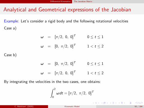
Example: Let’s consider a rigid body and the following rotational velocities
Case a)
ω = [π/2, 0, 0]T 0 ≤ t ≤ 1
ω = [0, π/2, 0]T 1 < t ≤ 2
Case b)
ω = [0, π/2, 0]T 0 ≤ t ≤ 1
ω = [π/2, 0, 0]T 1 < t ≤ 2
By integrating the velocities in the two cases, one obtains:
∫ 2
0
ωdt = [π/2, π/2, 0]T
C. Melchiorri (DEIS) Kinematic Model 93 / 164
Differential Kinematics The Jacobian Matrix
Analytical and Geometrical expressions of the Jacobian
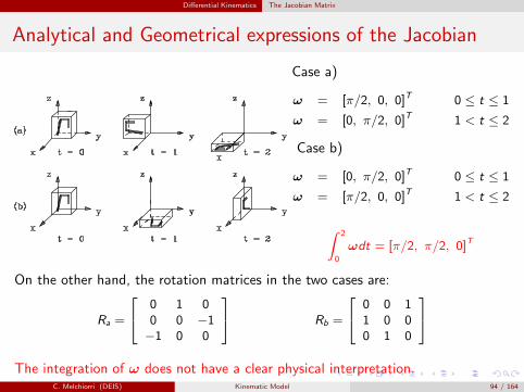
Case a)
ω = [π/2, 0, 0]T 0 ≤ t ≤ 1
ω = [0, π/2, 0]T 1 < t ≤ 2
Case b)
ω = [0, π/2, 0]T 0 ≤ t ≤ 1
ω = [π/2, 0, 0]T 1 < t ≤ 2
∫ 2
0
ωdt = [π/2, π/2, 0]T
On the other hand, the rotation matrices in the two cases are:
Ra =
0 1 00 0 −1−1 0 0
Rb =
0 0 11 0 00 1 0
The integration of ω does not have a clear physical interpretation.C. Melchiorri (DEIS) Kinematic Model 94 / 164
Differential Kinematics The Jacobian Matrix
Analytical and Geometrical expressions of the Jacobian
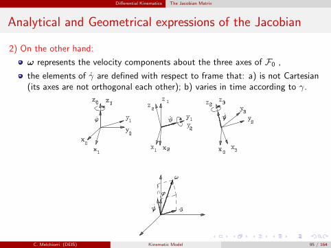
2) On the other hand:
ω represents the velocity components about the three axes of F0 ,
the elements of γ are defined with respect to frame that: a) is not Cartesian(its axes are not orthogonal each other); b) varies in time according to γ.
C. Melchiorri (DEIS) Kinematic Model 95 / 164
Differential Kinematics The Jacobian Matrix
Analytical and Geometrical expressions of the Jacobian
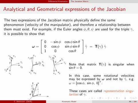
The two expressions of the Jacobian matrix physically define the samephenomenon (velocity of the manipulator), and therefore a relationship betweenthem must exist. For example, if the Euler angles φ, θ, ψ are used for the triple γ,it is possible to show that
ω =
0 − sinφ cosφ sin θ0 cosφ sinφ sin θ1 0 cos θ
γ = T(γ) γ
Note that matrix T(γ) is singular whensin θ = 0.
In this case, some rotational velocitiesmay be expressed by ω and not by γ, e.g.ω = [cosφ, sin φ, 0]T .
These cases are called representation singu-larities of γ.
C. Melchiorri (DEIS) Kinematic Model 96 / 164
Differential Kinematics The Jacobian Matrix
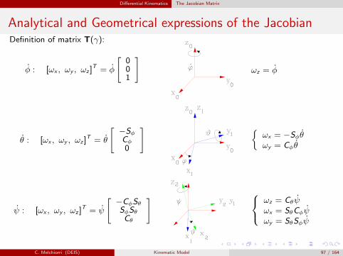
Analytical and Geometrical expressions of the JacobianDefinition of matrix T(γ):
φ : [ωx , ωy , ωz ]T = φ
[
001
]
ωz = φ
θ : [ωx , ωy , ωz ]T = θ
[
−Sφ
Cφ
0
]
{
ωx = −Sφθωy = Cφθ
ψ : [ωx , ωy , ωz ]T = ψ
[
−CφSθ
SφSθ
Cθ
]
ωz = Cθψωx = SθCφψωy = SθSφψ
C. Melchiorri (DEIS) Kinematic Model 97 / 164
Differential Kinematics The Jacobian Matrix
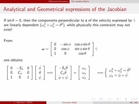
Analytical and Geometrical expressions of the Jacobian
If sin θ = 0, then the components perpendicular to z of the velocity expressed by γare linearly dependent (ω2
x + ω2y = θ2), while physically this constraint may not
exist!
From:
ω =
0 − sinφ cosφ sin θ0 cosφ sinφ sin θ1 0 cos θ
γ
one obtains:
0 −Sφ 00 Cφ 01 0 1
φ
θ
ψ
=⇒
−Sφθ
Cφθ
φ+ ψ
=
ωx
ωy
ωz
=⇒
{
ω2x + ω2
y = θ2
ωz = φ+ ψ
C. Melchiorri (DEIS) Kinematic Model 98 / 164
Differential Kinematics The Jacobian Matrix
Analytical and Geometrical expressions of the Jacobian
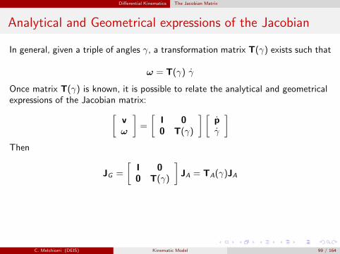
In general, given a triple of angles γ, a transformation matrix T(γ) exists such that
ω = T(γ) γ
Once matrix T(γ) is known, it is possible to relate the analytical and geometricalexpressions of the Jacobian matrix:
[
vω
]
=
[
I 00 T(γ)
] [
pγ
]
Then
JG =
[
I 00 T(γ)
]
JA = TA(γ)JA
C. Melchiorri (DEIS) Kinematic Model 99 / 164
Differential Kinematics Analytical Jacobian
Analitycal Jacobian
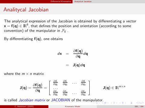
The analytical expression of the Jacobian is obtained by differentiating a vectorx = f(q) ∈ IR
6, that defines the position and orientation (according to someconvention) of the manipulator in F0 .
By differentiating f(q), one obtains
dx =∂f(q)
∂qdq
= J(q)dq
where the m × n matrix
J(q) =∂f(q)
∂q=
∂f1∂q1
∂f1∂q2
. . . ∂f1∂qn
. . .∂fm∂q1
∂fm∂q2
. . . ∂fm∂qn
J(q) ∈ IRm×n
is called Jacobian matrix or JACOBIAN of the manipulator.
C. Melchiorri (DEIS) Kinematic Model 100 / 164
Differential Kinematics Analytical Jacobian
Analitycal Jacobian
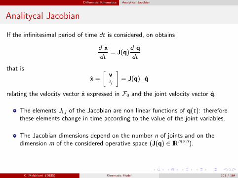
If the infinitesimal period of time dt is considered, on obtains
d x
dt= J(q)
d q
dt
that is
x =
[
vγ
]
= J(q) q
relating the velocity vector x expressed in F0 and the joint velocity vector q.
The elements Ji ,j of the Jacobian are non linear functions of q(t): thereforethese elements change in time according to the value of the joint variables.
The Jacobian dimensions depend on the number n of joints and on thedimension m of the considered operative space (J(q) ∈ IR
m×n).
C. Melchiorri (DEIS) Kinematic Model 101 / 164
Differential Kinematics Analytical Jacobian
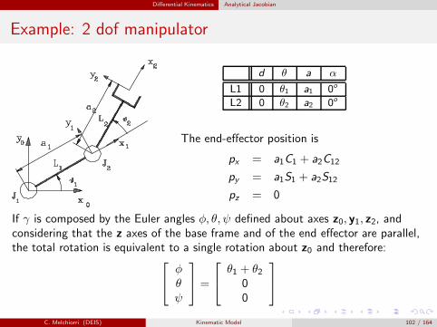
Example: 2 dof manipulator
d θ a α
L1 0 θ1 a1 0o
L2 0 θ2 a2 0o
The end-effector position is
px = a1C1 + a2C12
py = a1S1 + a2S12
pz = 0
If γ is composed by the Euler angles φ, θ, ψ defined about axes z0, y1, z2, andconsidering that the z axes of the base frame and of the end effector are parallel,the total rotation is equivalent to a single rotation about z0 and therefore:
φθψ
=
θ1 + θ200
C. Melchiorri (DEIS) Kinematic Model 102 / 164
Differential Kinematics Analytical Jacobian
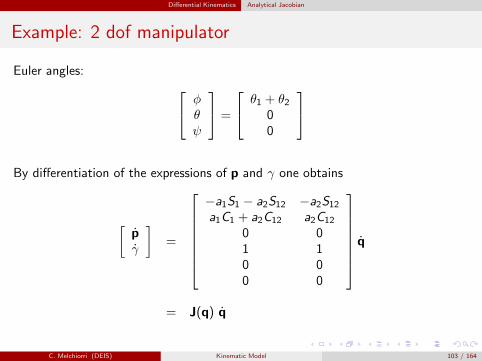
Example: 2 dof manipulator
Euler angles:
φθψ
=
θ1 + θ200
By differentiation of the expressions of p and γ one obtains
[
pγ
]
=
−a1S1 − a2S12 −a2S12a1C1 + a2C12 a2C12
0 01 10 00 0
q
= J(q) q
C. Melchiorri (DEIS) Kinematic Model 103 / 164
Differential Kinematics Geometric Jacobian
Geometric Expression of the Jacobian
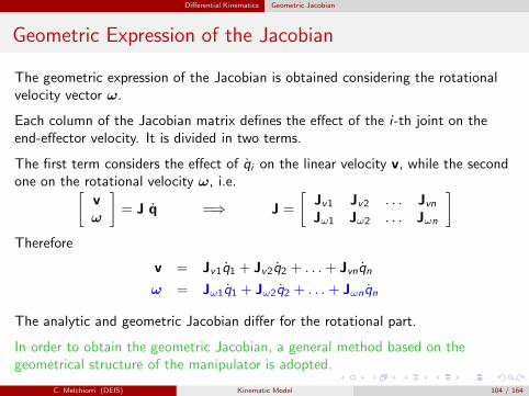
The geometric expression of the Jacobian is obtained considering the rotationalvelocity vector ω.
Each column of the Jacobian matrix defines the effect of the i-th joint on theend-effector velocity. It is divided in two terms.
The first term considers the effect of qi on the linear velocity v, while the secondone on the rotational velocity ω, i.e.
[
vω
]
= J q =⇒ J =
[
Jv1 Jv2 . . . JvnJω1 Jω2 . . . Jωn
]
Therefore
v = Jv1q1 + Jv2q2 + . . .+ Jvnqn
ω = Jω1q1 + Jω2q2 + . . .+ Jωnqn
The analytic and geometric Jacobian differ for the rotational part.
In order to obtain the geometric Jacobian, a general method based on thegeometrical structure of the manipulator is adopted.
C. Melchiorri (DEIS) Kinematic Model 104 / 164
Differential Kinematics Geometric Jacobian
Derivative of a Rotation Matrix
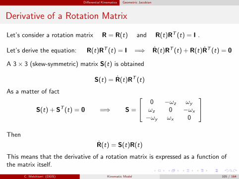
Let’s consider a rotation matrix R = R(t) and R(t)RT (t) = I .
Let’s derive the equation: R(t)RT (t) = I =⇒ R(t)RT (t) + R(t)RT (t) = 0
A 3× 3 (skew-symmetric) matrix S(t) is obtained
S(t) = R(t)RT (t)
As a matter of fact
S(t) + ST (t) = 0 =⇒ S =
0 −ωz ωy
ωz 0 −ωx
−ωy ωx 0
Then
R(t) = S(t)R(t)
This means that the derivative of a rotation matrix is expressed as a function ofthe matrix itself.
C. Melchiorri (DEIS) Kinematic Model 105 / 164
Differential Kinematics Geometric Jacobian
Derivative of a Rotation Matrix
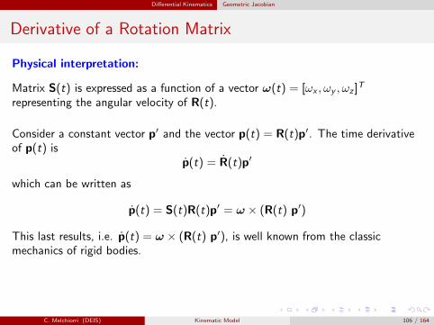
Physical interpretation:
Matrix S(t) is expressed as a function of a vector ω(t) = [ωx , ωy , ωz ]T
representing the angular velocity of R(t).
Consider a constant vector p′ and the vector p(t) = R(t)p′. The time derivativeof p(t) is
p(t) = R(t)p′
which can be written as
p(t) = S(t)R(t)p′ = ω × (R(t) p′)
This last results, i.e. p(t) = ω × (R(t) p′), is well known from the classicmechanics of rigid bodies.
C. Melchiorri (DEIS) Kinematic Model 106 / 164
Differential Kinematics Geometric Jacobian
Derivative of a Rotation Matrix
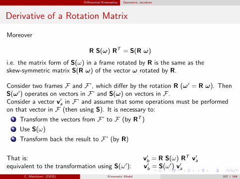
Moreover
R S(ω) RT = S(R ω)
i.e. the matrix form of S(ω) in a frame rotated by R is the same as theskew-symmetric matrix S(R ω) of the vector ω rotated by R.
Consider two frames F and F ’, which differ by the rotation R (ω′ = R ω). ThenS(ω′) operates on vectors in F ’ and S(ω) on vectors in F .Consider a vector v′a in F ’ and assume that some operations must be performedon that vector in F (then using S). It is necessary to:
1 Transform the vectors from F ’ to F (by RT )
2 Use S(ω)
3 Transform back the result to F ’ (by R)
That is: v′b = R S(ω) RT v′aequivalent to the transformation using S(ω′): v′b = S(ω′) v′a
C. Melchiorri (DEIS) Kinematic Model 107 / 164
Differential Kinematics Geometric Jacobian
Example
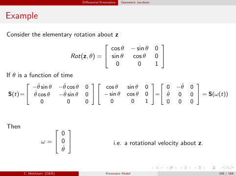
Consider the elementary rotation about z
Rot(z, θ) =
cos θ − sin θ 0sin θ cos θ 00 0 1
If θ is a function of time
S(t)=
−θ sin θ −θ cos θ 0
θ cos θ −θ sin θ 00 0 0
cos θ sin θ 0− sin θ cos θ 0
0 0 1
=
0 −θ 0
θ 0 00 0 0
= S(ω(t))
Then
ω =
00
θ
i.e. a rotational velocity about z.
C. Melchiorri (DEIS) Kinematic Model 108 / 164
Differential Kinematics Geometric Jacobian
Geometric Jacobian
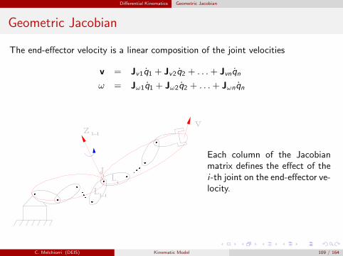
The end-effector velocity is a linear composition of the joint velocities
v = Jv1q1 + Jv2q2 + . . .+ Jvnqn
ω = Jω1q1 + Jω2q2 + . . .+ Jωnqn
Each column of the Jacobianmatrix defines the effect of thei-th joint on the end-effector ve-locity.
C. Melchiorri (DEIS) Kinematic Model 109 / 164
Differential Kinematics Geometric Jacobian
Geometric Jacobian
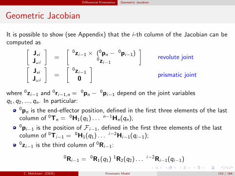
It is possible to show (see Appendix) that the i-th column of the Jacobian can becomputed as
[
JviJωi
]
=
[
0zi−1 × (0pn −0pi−1)
0zi−1
]
revolute joint
[
JviJωi
]
=
[
0zi−1
0
]
prismatic joint
where 0zi−1 and 0ri−1,n =0pn −
0pi−1 depend on the joint variablesq1, q2, ..., qn. In particular:
0pn is the end-effector position, defined in the first three elements of the lastcolumn of 0Tn = 0H1(q1) . . .
n−1Hn(qn);0pi−1 is the position of F i−1, defined in the first three elements of the lastcolumn of 0Ti−1 =
0H1(q1) . . .i−2Hi−1(qi−1);
0zi−1 is the third column of 0Ri−1:
0Ri−1 =0R1(q1)
1R2(q2) . . .i−2Ri−1(qi−1)
C. Melchiorri (DEIS) Kinematic Model 110 / 164
Differential Kinematics Examples
Example: 2 dof manipulator
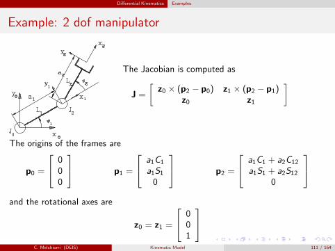
The Jacobian is computed as
J =
[
z0 × (p2 − p0) z1 × (p2 − p1)z0 z1
]
The origins of the frames are
p0 =
000
p1 =
a1C1
a1S10
p2 =
a1C1 + a2C12
a1S1 + a2S120
and the rotational axes are
z0 = z1 =
001
C. Melchiorri (DEIS) Kinematic Model 111 / 164
Differential Kinematics Examples
Example: 2 dof manipulator
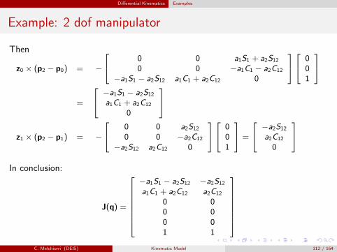
Then
z0 × (p2 − p0) = −
0 0 a1S1 + a2S12
0 0 −a1C1 − a2C12
−a1S1 − a2S12 a1C1 + a2C12 0
001
=
−a1S1 − a2S12
a1C1 + a2C12
0
z1 × (p2 − p1) = −
0 0 a2S12
0 0 −a2C12
−a2S12 a2C12 0
001
=
−a2S12
a2C12
0
In conclusion:
J(q) =
−a1S1 − a2S12 −a2S12
a1C1 + a2C12 a2C12
0 00 00 01 1
C. Melchiorri (DEIS) Kinematic Model 112 / 164
Differential Kinematics Examples
Example: 2 dof manipulator
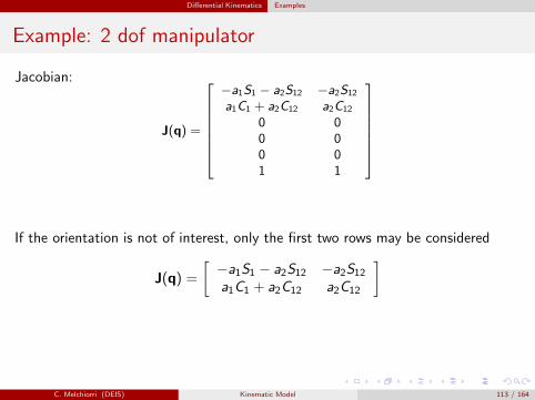
Jacobian:
J(q) =
−a1S1 − a2S12 −a2S12
a1C1 + a2C12 a2C12
0 00 00 01 1
If the orientation is not of interest, only the first two rows may be considered
J(q) =
[
−a1S1 − a2S12 −a2S12a1C1 + a2C12 a2C12
]
C. Melchiorri (DEIS) Kinematic Model 113 / 164
Differential Kinematics Examples
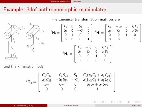
Example: 3dof anthropomorphic manipulator
The canonical transformation matrices are
0H1=
C1 0 S1 0S1 0 −C1 00 1 0 00 0 0 1
1H2=
C2 −S2 0 a2C2
S2 C2 0 a2S2
0 0 1 00 0 0 1
2H3 =
C3 −S3 0 a3C3
S3 C3 0 a3S3
0 0 1 00 0 0 1
and the kinematic model
0T3 =
C1C23 −C1S23 S1 C1(a2C2 + a3C23)S1C23 −S1S23 −C1 S1(a2C2 + a3C23)S23 C23 0 a2S2 + a3S230 0 0 1
C. Melchiorri (DEIS) Kinematic Model 114 / 164
Differential Kinematics Examples
Example: 3dof anthropomorphic manipulator
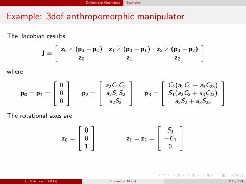
The Jacobian results
J =
[
z0 × (p3 − p0) z1 × (p3 − p1) z2 × (p3 − p2)z0 z1 z2
]
where
p0 = p1 =
000
p2 =
a2C1C2
a2S1S2a2S2
p3 =
C1(a2C2 + a3C23)S1(a2C2 + a3C23)a2S2 + a3S23
The rotational axes are
z0 =
001
z1 = z2 =
S1−C1
0
C. Melchiorri (DEIS) Kinematic Model 115 / 164
Differential Kinematics Examples
Example: 3dof anthropomorphic manipulator
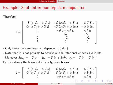
Therefore
J =
−S1(a2C2 + a3C23) −C1(a2S2 + a3S23) −a3C1S23C1(a2C2 + a3C23) −S1(a2S2 + a3S23) −a3S1S23
0 a2C2 + a3C23 a3C23
0 S1 S10 −C1 −C1
1 0 0
- Only three rows are linearly independent (3 dof).
- Note that it is not possible to achieve all the rotational velocities ω in IR3.
- Moreover S1ωy = −C1ωx (ωx = S1θ2 + S1θ3, ωy = −C1θ2 − C1θ3, ).
By considering the linear velocity only, one obtains:
J =
−S1(a2C2 + a3C23) −C1(a2S2 + a3S23) −a3C1S23C1(a2C2 + a3C23) −S1(a2S2 + a3S23) −a3S1S23
0 a2C2 + a3C23 a3C23
C. Melchiorri (DEIS) Kinematic Model 116 / 164
Differential Kinematics Examples
Example: 3dof anthropomorphic manipulator
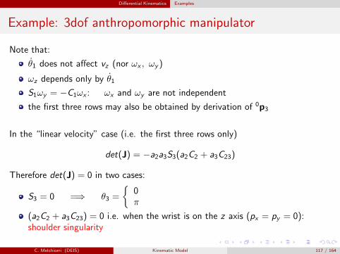
Note that:
θ1 does not affect vz (nor ωx , ωy )
ωz depends only by θ1
S1ωy = −C1ωx : ωx and ωy are not independent
the first three rows may also be obtained by derivation of 0p3
In the “linear velocity” case (i.e. the first three rows only)
det(J) = −a2a3S3(a2C2 + a3C23)
Therefore det(J) = 0 in two cases:
S3 = 0 =⇒ θ3 =
{
0π
(a2C2 + a3C23) = 0 i.e. when the wrist is on the z axis (px = py = 0):shoulder singularity
C. Melchiorri (DEIS) Kinematic Model 117 / 164
Differential Kinematics Examples
Example 3 dof spherical manipulator
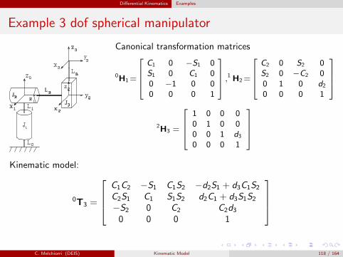
Canonical transformation matrices
0H1=
C1 0 −S1 0S1 0 C1 00 −1 0 00 0 0 1
,1 H2=
C2 0 S2 0S2 0 −C2 00 1 0 d20 0 0 1
2H3 =
1 0 0 00 1 0 00 0 1 d30 0 0 1
Kinematic model:
0T3 =
C1C2 −S1 C1S2 −d2S1 + d3C1S2C2S1 C1 S1S2 d2C1 + d3S1S2−S2 0 C2 C2d30 0 0 1
C. Melchiorri (DEIS) Kinematic Model 118 / 164
Differential Kinematics Examples
Example 3 dof spherical manipulator
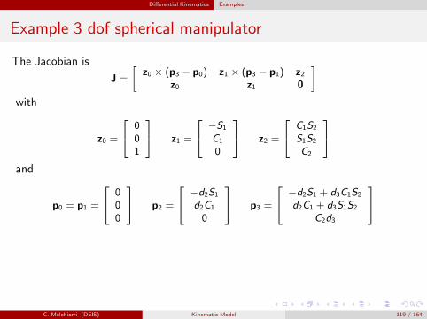
The Jacobian is
J =
[
z0 × (p3 − p0) z1 × (p3 − p1) z2z0 z1 0
]
with
z0 =
001
z1 =
−S1
C1
0
z2 =
C1S2
S1S2
C2
and
p0 = p1 =
000
p2 =
−d2S1
d2C1
0
p3 =
−d2S1 + d3C1S2
d2C1 + d3S1S2
C2d3
C. Melchiorri (DEIS) Kinematic Model 119 / 164
Differential Kinematics Examples
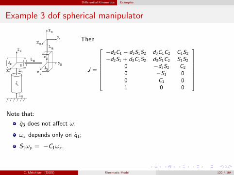
Example 3 dof spherical manipulator
Then
J =
−d2C1 − d3S1S2 d3C1C2 C1S2
−d2S1 + d3C1S2 d3S1C2 S1S2
0 −d3S2 C2
0 −S1 00 C1 01 0 0
Note that:
q3 does not affect ω;
ωz depends only on q1;
S1ωy = −C1ωx .
C. Melchiorri (DEIS) Kinematic Model 120 / 164
Differential Kinematics Examples
Example: 3 dof spherical wrist
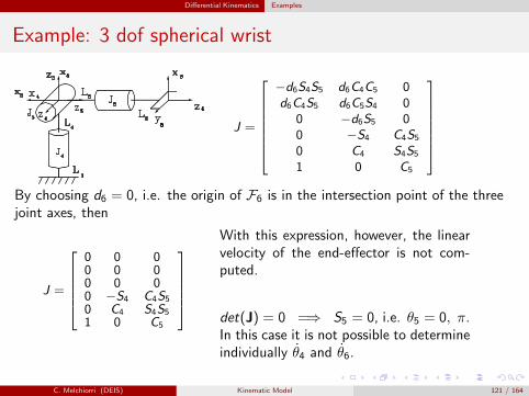
J =
−d6S4S5 d6C4C5 0d6C4S5 d6C5S4 0
0 −d6S5 00 −S4 C4S5
0 C4 S4S5
1 0 C5
By choosing d6 = 0, i.e. the origin of F6 is in the intersection point of the threejoint axes, then
J =
0 0 00 0 00 0 00 −S4 C4S5
0 C4 S4S5
1 0 C5
With this expression, however, the linearvelocity of the end-effector is not com-puted.
det(J) = 0 =⇒ S5 = 0, i.e. θ5 = 0, π.In this case it is not possible to determineindividually θ4 and θ6.
C. Melchiorri (DEIS) Kinematic Model 121 / 164
Differential Kinematics Examples
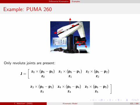
Example: PUMA 260
Only revolute joints are present:
J =
[
z0 × (p6 − p0) z1 × (p6 − p1) z2 × (p6 − p2)z0 z1 z2
z3 × (p6 − p3) z4 × (p6 − p4) z5 × (p6 − p5)z3 z4 z5
]
C. Melchiorri (DEIS) Kinematic Model 122 / 164
Differential Kinematics Examples
Example: PUMA 260
If d6 = 0:
J =
−d3C1 − S1(a2C2 + d4S23) C1(d4C23 − a2S2) d4C1C23
−d3S1 + C1(a2C2 + d4S23) S1(d4C23 − a2S2) d4S1C23
0 a2C2 + d4S23 d4S23
0 S1 S1
0 −C1 −C1
1 0 0
0 0 00 0 00 0 0
C1S23 S1C4 − C1C23S4 C1S23C5 + C1C23C4S5 + S1S4S5
S1S23 −C1C4 − S1C23S4 S1S23C5 + S1C23C4S5 − C1S4S5
−C23 −S23S4 −C23C5 + S23C4S5
C. Melchiorri (DEIS) Kinematic Model 123 / 164
Statics - Singularities - Inverse differential kinematics
Kinematic Model of Robot ManipulatorsStatics - Singularities - Inverse differential kinematics
Claudio Melchiorri
Dipartimento di Ingegneria dell’Energia Elettrica e dell’Informazione (DEI)
Universita di Bologna
email: [email protected]
C. Melchiorri (DEIS) Kinematic Model 124 / 164
Statics - Singularities - Inverse differential kinematics Statics
Forces
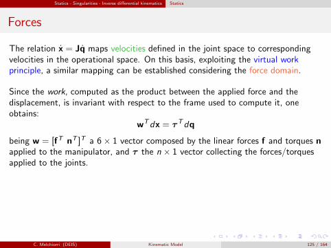
The relation x = Jq maps velocities defined in the joint space to correspondingvelocities in the operational space. On this basis, exploiting the virtual workprinciple, a similar mapping can be established considering the force domain.
Since the work, computed as the product between the applied force and thedisplacement, is invariant with respect to the frame used to compute it, oneobtains:
wTdx = τTdq
being w = [fT nT ]T a 6× 1 vector composed by the linear forces f and torques napplied to the manipulator, and τ the n × 1 vector collecting the forces/torquesapplied to the joints.
C. Melchiorri (DEIS) Kinematic Model 125 / 164
Statics - Singularities - Inverse differential kinematics Statics
Forces
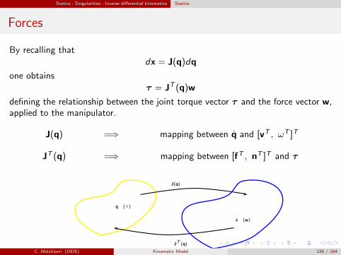
By recalling that
dx = J(q)dq
one obtains
τ = JT (q)w
defining the relationship between the joint torque vector τ and the force vector w,applied to the manipulator.
J(q) =⇒ mapping between q and [vT , ωT ]T
JT (q) =⇒ mapping between [fT , nT ]T and τ
q (τ)
J(q)
JT (q)
x (w)
C. Melchiorri (DEIS) Kinematic Model 126 / 164
Statics - Singularities - Inverse differential kinematics Transformation of reference frame for the Jacobian
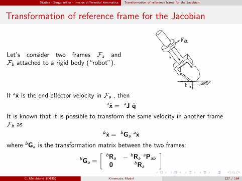
Transformation of reference frame for the Jacobian
Let’s consider two frames Fa andFb attached to a rigid body (“robot”).
If ax is the end-effector velocity in Fa , thenax = aJ q
It is known that it is possible to transform the same velocity in another frameFb as
bx = bGaax
where bGa is the transformation matrix between the two frames:
bGa =
[
bRa − bRaaPab
0 bRa
]
C. Melchiorri (DEIS) Kinematic Model 127 / 164
Statics - Singularities - Inverse differential kinematics Transformation of reference frame for the Jacobian
Transformation of reference frame for the Jacobian
Thenbx = bJ q = bGa
ax = bGaaJ q
and therefore the transformation for the Jacobian between the two frames Fa andFb is given by
bJ = bGaaJ
Similar considerations hold in the force domain (where the transpose Jacobian isused).
Note that if the two frames are not rigidly attached to the robot, then theJacobian transformation between them is defined only by the rotation matrix bRa:
bJ =
[
bRa 00 bRa
]
aJ
C. Melchiorri (DEIS) Kinematic Model 128 / 164
Statics - Singularities - Inverse differential kinematics Kinematic singularities
Singular configurations
The Jacobian is a 6× n matrix mapping the IRn joint velocity space to the IR
6
operational velocity space:
x = J(q)q
From an infinitesimal point of view, this relationship is expressed as
dx = J(q)dq
that can be interpreted as a relationship between infinitesimal displacements inIR
n and IR6.
Singular configurations or Singulariities
In general, rank(J(q)) = min (6, n). On the other hand, since the elements of Jare function of the joints, some robot configurations exist such that the Jacobianlooses rank. These configurations are denoted as kinematic singularities.In these configurations, there are “directions” (vectors x) in IR
6 without anycorrespondent “direction” (q) in IR
n: these directions cannot be actuated and therobot ”looses” a motion capability.
C. Melchiorri (DEIS) Kinematic Model 129 / 164
Statics - Singularities - Inverse differential kinematics Kinematic singularities
Singular configurations
The singular configurations are important for several reasons:
1 They represents configurations in which the motion capabilities of the robot arereduced: it is not possible to impose arbitrary motions of the end-effector
2 In the proximity of a singularity, small velocities in the operational space maygenerate large (infinite) velocities in the joint space
3 They correspond to configurations that have not a well defined solution to theinverse kinematic problem: either no solution or infinite solutions.
There are two types of singularities:
1 Boundary singularities, that correspond to points on the border of the workspace,i.e. when the robot is either fully extended or retracted. These singularities may beeasily avoided by not driving the manipulator to the border of its workspace
2 Internal singularities, that occur inside the reachable workspace and are generallycaused by the alignment of two or more axes of motion, or else by the attainmentof particular end-effector configurations. These singularities constitute a seriousproblem, as they can be encountered anywhere in the reachable workspace for aplanned path in the operational space.
C. Melchiorri (DEIS) Kinematic Model 130 / 164
Statics - Singularities - Inverse differential kinematics Kinematic singularities
Example
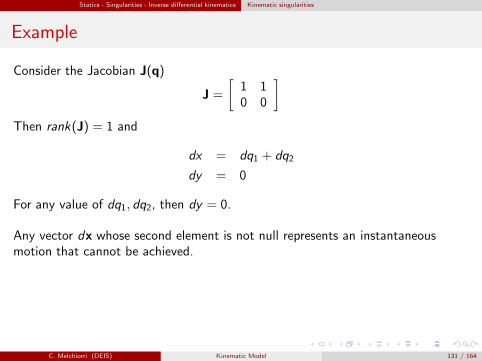
Consider the Jacobian J(q)
J =
[
1 10 0
]
Then rank(J) = 1 and
dx = dq1 + dq2
dy = 0
For any value of dq1, dq2, then dy = 0.
Any vector dx whose second element is not null represents an instantaneousmotion that cannot be achieved.
C. Melchiorri (DEIS) Kinematic Model 131 / 164
Statics - Singularities - Inverse differential kinematics Kinematic singularities
Example
Jacobian:
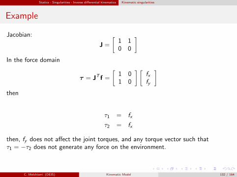
J =
[
1 10 0
]
In the force domain
τ = JT f =
[
1 01 0
] [
fxfy
]
then
τ1 = fx
τ2 = fx
then, fy does not affect the joint torques, and any torque vector such thatτ1 = −τ2 does not generate any force on the environment.
C. Melchiorri (DEIS) Kinematic Model 132 / 164

Statics - Singularities - Inverse differential kinematics Kinematic singularities
Example
Consider the 2 dof planar manipulator:
J(q) =
[
−a1S1 − a2S12 −a2S12a1C1 + a2C12 a2C12
]
If θ1 = θ2 = 0, then
J(q) =
[
0 0a1 + a2 a2
]
=
[
0 02 1
]
if a1 = a2 = 1
Therefore{
dx = 0dy = 2 dq1 + dq2
Moreover
JT (q) =
[
0 20 1
]
=⇒
{
τ1 = 2 fyτ2 = fy
If τ2 = −2 τ1 → fx = fy = 0.
C. Melchiorri (DEIS) Kinematic Model 133 / 164
Statics - Singularities - Inverse differential kinematics Kinematic singularities
Example
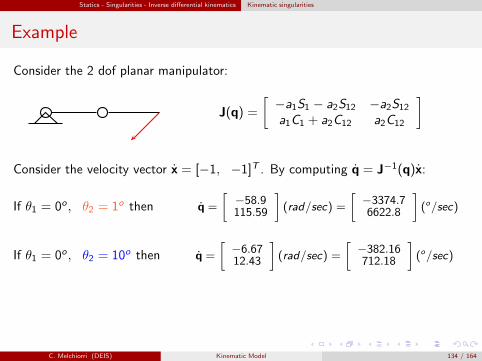
Consider the 2 dof planar manipulator:
J(q) =
[
−a1S1 − a2S12 −a2S12a1C1 + a2C12 a2C12
]
Consider the velocity vector x = [−1, −1]T . By computing q = J−1(q)x:
If θ1 = 0o , θ2 = 1o then q =
[
−58.9115.59
]
(rad/sec) =
[
−3374.76622.8
]
(o/sec)
If θ1 = 0o , θ2 = 10o then q =
[
−6.6712.43
]
(rad/sec) =
[
−382.16712.18
]
(o/sec)
C. Melchiorri (DEIS) Kinematic Model 134 / 164
Statics - Singularities - Inverse differential kinematics Kinematic singularities
Example
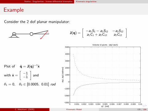
Consider the 2 dof planar manipulator:
J(q) =
[
−a1S1 − a2S12 −a2S12
a1C1 + a2C12 a2C12
]
Plot of q = J(q)−1x
with x =
[
−1−1
]
and
θ1 = 0, θ2 ∈ [0.0005, 0.01] rad
0 0.001 0.002 0.003 0.004 0.005 0.006 0.007 0.008 0.009 0.01−3000
−2000
−1000
0
1000
2000
3000
4000
5000
q2 [rad]
dq1,
dq2
[rad
/sec
]
Velocita‘ di giunto (dq2 dash)
C. Melchiorri (DEIS) Kinematic Model 135 / 164
Statics - Singularities - Inverse differential kinematics Kinematic singularities
Singularity decoupling
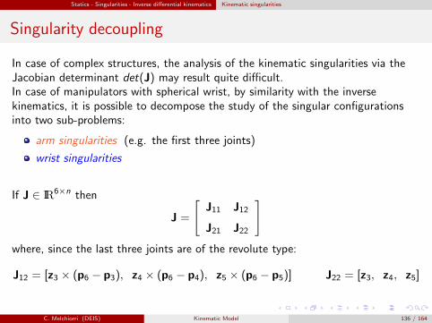
In case of complex structures, the analysis of the kinematic singularities via theJacobian determinant det(J) may result quite difficult.In case of manipulators with spherical wrist, by similarity with the inversekinematics, it is possible to decompose the study of the singular configurationsinto two sub-problems:
arm singularities (e.g. the first three joints)
wrist singularities
If J ∈ IR6×n then
J =
[
J11 J12
J21 J22
]
where, since the last three joints are of the revolute type:
J12 = [z3 × (p6 − p3), z4 × (p6 − p4), z5 × (p6 − p5)] J22 = [z3, z4, z5]
C. Melchiorri (DEIS) Kinematic Model 136 / 164
Statics - Singularities - Inverse differential kinematics Kinematic singularities
Singularity decoupling
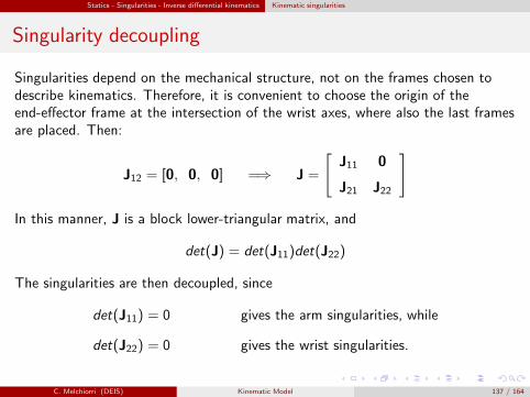
Singularities depend on the mechanical structure, not on the frames chosen todescribe kinematics. Therefore, it is convenient to choose the origin of theend-effector frame at the intersection of the wrist axes, where also the last framesare placed. Then:
J12 = [0, 0, 0] =⇒ J =
[
J11 0
J21 J22
]
In this manner, J is a block lower-triangular matrix, and
det(J) = det(J11)det(J22)
The singularities are then decoupled, since
det(J11) = 0 gives the arm singularities, while
det(J22) = 0 gives the wrist singularities.
C. Melchiorri (DEIS) Kinematic Model 137 / 164
Statics - Singularities - Inverse differential kinematics Inverse Differential Kinematics
Inverse Differential Kinematics
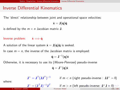
The ‘direct’ relationship between joint and operational space velocities:
x = J(q)q
is defined by the m × n Jacobian matrix J.
Inverse problem: x =⇒ q
A solution of the linear system x = J(q)q is seeked.
In case m = n, the inverse of the Jacobian matrix is employed:
q = J−1(q)x
Otherwise, it is necessary to use its (Moore-Penrose) pseudo-inverse
q = J+(q)x
where:J+ = JT (JJT )−1 if m < n (right pseudo-inverse : JJ+ = I)
J+ = (JTJ)−1JT if m > n (left pseudo-inverse: J+J = I)C. Melchiorri (DEIS) Kinematic Model 138 / 164
Statics - Singularities - Inverse differential kinematics Inverse Differential Kinematics
Inverse Differential Kinematics
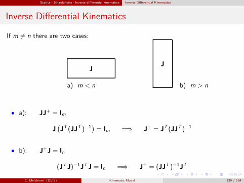
If m 6= n there are two cases:
J
a) m < n
J
b) m > n
• a): JJ+ = Im
J(
JT (JJT )−1)
= Im =⇒ J+ = JT (JJT )−1
• b): J+J = In
(JTJ)−1JTJ = In =⇒ J+ = (JJT )−1JT
C. Melchiorri (DEIS) Kinematic Model 139 / 164
Statics - Singularities - Inverse differential kinematics Inverse Differential Kinematics
Inverse Differential Kinematics
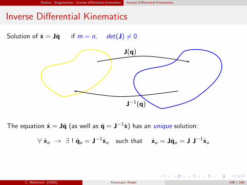
Solution of x = Jq if m = n, det(J) 6= 0
J(q)
J−1(q)
The equation x = Jq (as well as q = J−1x) has an unique solution:
∀ xo → ∃ ! qo = J−1xo such that xo = Jqo = J J−1xo
C. Melchiorri (DEIS) Kinematic Model 140 / 164
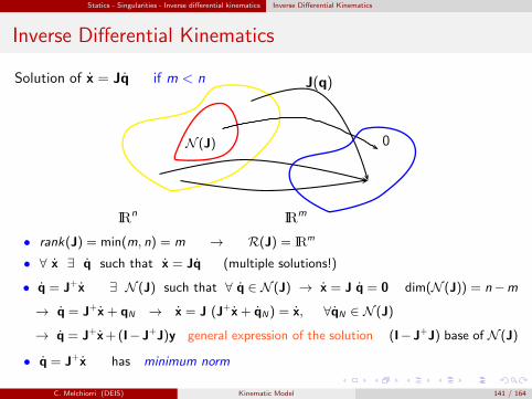
Statics - Singularities - Inverse differential kinematics Inverse Differential Kinematics
Inverse Differential Kinematics
Solution of x = Jq if m < n
N (J)
IRn
0
J(q)
IRm
• rank(J) = min(m, n) = m → R(J) = IRm
• ∀ x ∃ q such that x = Jq (multiple solutions!)
• q = J+x ∃ N (J) such that ∀ q ∈ N (J) → x = J q = 0 dim(N (J)) = n−m
→ q = J+x+ qN → x = J (J+x+ qN) = x, ∀qN ∈ N (J)
→ q = J+x+(I−J+J)y general expression of the solution (I−J+J) base of N (J)
• q = J+x has minimum norm
C. Melchiorri (DEIS) Kinematic Model 141 / 164
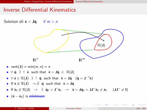
Statics - Singularities - Inverse differential kinematics Inverse Differential Kinematics
Inverse Differential Kinematics
Solution ofi x = Jq if m > n
IRn
R(J)
IRm
• rank(J) = min(m, n) = n
• ∀ q ∃ ! x such that x = Jq ∈ R(J)
• ∀ x ∈ R(J) ∃ ! q such that x = Jq (q = J−1x)
• If x 6∈ R(J) →6 ∃ q such that x = Jq
• If x0 6∈ R(J) → ∃ q0 = J+x0 → x = Jq0 = JJ+x0 6= x0 (JJ+ 6= I)
• ‖x− x0‖ is minimum
C. Melchiorri (DEIS) Kinematic Model 142 / 164
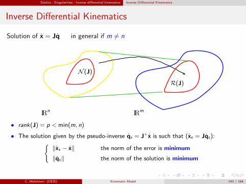
Statics - Singularities - Inverse differential kinematics Inverse Differential Kinematics
Inverse Differential Kinematics
Solution of x = Jq in general if m 6= n
N (J)
IRn
R(J)
IRm
• rank(J) = p < min(m, n)
• The solution given by the pseudo-inverse qs = J+x is such that (xs = Jqs):{
‖xs − x‖ the norm of the error is minimum
‖qs‖ the norm of the solution is minimum
C. Melchiorri (DEIS) Kinematic Model 143 / 164
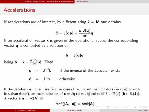
Statics - Singularities - Inverse differential kinematics Accelerations
Accelerations
If accelerations are of interest, by differentiating x = Jq one obtains
x = J(q)q+d J(q)
dtq
If an acceleration vector x is given in the operational space, the correspondingvector q is computed as a solution of
b = J(q)q
being b = x− d J(q)dt
q. Then
q = J−1b if the inverse of the Jacobian exists
q = J+b otherwise
If the Jacobian is not square (e.g. in case of redundant manipulators (m < n) or withless than 6 dof), an exact solution of x = Jq (b = Jq) exists iff x ∈ R(J) (b ∈ R(J)).A vector a is in R(A) iff
rank([A, a]) = rank[A]
C. Melchiorri (DEIS) Kinematic Model 144 / 164
Inverse kinematics algorithms
Kinematic Model of Robot ManipulatorsInverse kinematics algorithms
Claudio Melchiorri
Dipartimento di Ingegneria dell’Energia Elettrica e dell’Informazione (DEI)
Universita di Bologna
email: [email protected]
C. Melchiorri (DEIS) Kinematic Model 145 / 164
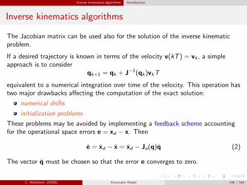
Inverse kinematics algorithms Introduction
Inverse kinematics algorithms
The Jacobian matrix can be used also for the solution of the inverse kinematicproblem.
If a desired trajectory is known in terms of the velocity v(kT ) = vk , a simpleapproach is to consider
qk+1 = qk + J−1(qk)vkT
equivalent to a numerical integration over time of the velocity. This operation hastwo major drawbacks affecting the computation of the exact solution:
numerical drifts
initialization problems
These problems may be avoided by implementing a feedback scheme accountingfor the operational space errors e = xd − x. Then
e = xd − x = xd − Ja(q)q (2)
The vector q must be chosen so that the error e converges to zero.
C. Melchiorri (DEIS) Kinematic Model 146 / 164
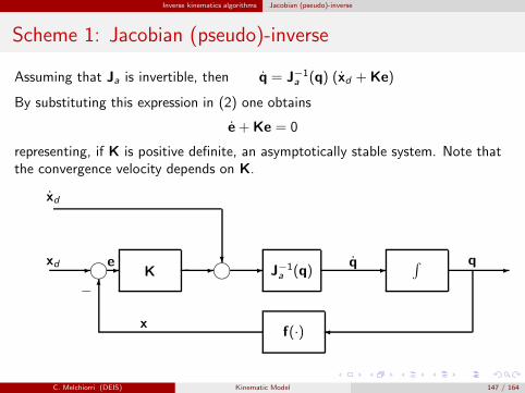
Inverse kinematics algorithms Jacobian (pseudo)-inverse
Scheme 1: Jacobian (pseudo)-inverse
Assuming that Ja is invertible, then q = J−1a (q) (xd +Ke)
By substituting this expression in (2) one obtains
e+Ke = 0
representing, if K is positive definite, an asymptotically stable system. Note thatthe convergence velocity depends on K.
K J−1a (q)
∫
f(·)
❥❥ ✲ ✲
✛
✲✲✲✲
✻
❄
−
xd
xd
e q q
x
C. Melchiorri (DEIS) Kinematic Model 147 / 164
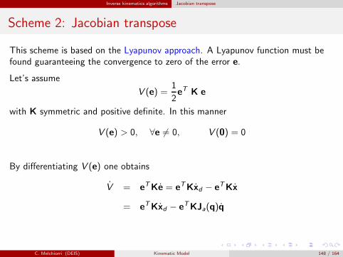
Inverse kinematics algorithms Jacobian transpose
Scheme 2: Jacobian transpose
This scheme is based on the Lyapunov approach. A Lyapunov function must befound guaranteeing the convergence to zero of the error e.
Let’s assume
V (e) =1
2eT K e
with K symmetric and positive definite. In this manner
V (e) > 0, ∀e 6= 0, V (0) = 0
By differentiating V (e) one obtains
V = eTKe = eTKxd − eTKx
= eTKxd − eTKJa(q)q
C. Melchiorri (DEIS) Kinematic Model 148 / 164
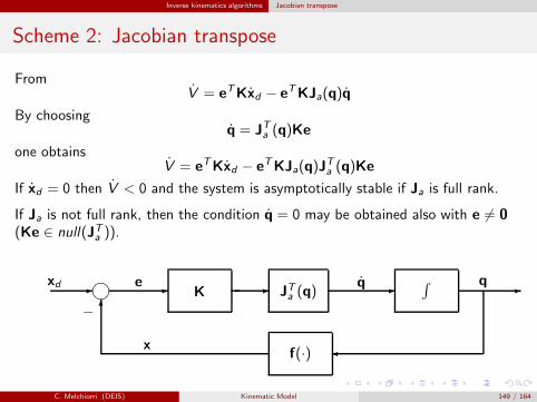
Inverse kinematics algorithms Jacobian transpose
Scheme 2: Jacobian transpose
FromV = eTKxd − eTKJa(q)q
By choosingq = JTa (q)Ke
one obtainsV = eTKxd − eTKJa(q)J
Ta (q)Ke
If xd = 0 then V < 0 and the system is asymptotically stable if Ja is full rank.
If Ja is not full rank, then the condition q = 0 may be obtained also with e 6= 0(Ke ∈ null(JTa )).
K JTa (q)∫
f(·)
❥ ✲ ✲
✛
✲✲
✻−
xd e q q
x
✲
C. Melchiorri (DEIS) Kinematic Model 149 / 164
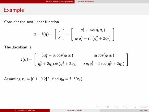
Inverse kinematics algorithms Jacobian transpose
Example
Consider the non linear function
z = f(q) =
[
xy
]
=
[
q31 + sin(q1q2)
q1q32 + sin(q21 + 2q2)
]
The Jacobian is
J(q) =
[
3q21 + q2cos(q1q2) q1cos(q1q2)
q32 + 2q1cos(q21 + 2q2) 3q1q
22 + 2cos(q21 + 2q2)
]
Assuming z0 = [0.1, 0.2]T , find q0 = f−1(z0).
C. Melchiorri (DEIS) Kinematic Model 150 / 164
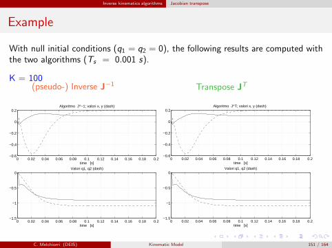
Inverse kinematics algorithms Jacobian transpose
Example
With null initial conditions (q1 = q2 = 0), the following results are computed withthe two algorithms (Ts = 0.001 s).
K = 100(pseudo-) Inverse J−1
0 0.02 0.04 0.06 0.08 0.1 0.12 0.14 0.16 0.18 0.2−0.6
−0.4
−0.2
0
0.2Algoritmo J^−1; valori x, y (dash)
time [s]
0 0.02 0.04 0.06 0.08 0.1 0.12 0.14 0.16 0.18 0.2−1.5
−1
−0.5
0Valori q1, q2 (dash)
time [s]
Transpose JT
0 0.02 0.04 0.06 0.08 0.1 0.12 0.14 0.16 0.18 0.2−0.6
−0.4
−0.2
0
0.2Algoritmo J^T; valori x, y (dash)
time [s]
0 0.02 0.04 0.06 0.08 0.1 0.12 0.14 0.16 0.18 0.2−1.5
−1
−0.5
0Valori q1, q2 (dash)
time [s]
C. Melchiorri (DEIS) Kinematic Model 151 / 164
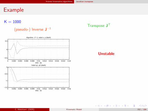
Inverse kinematics algorithms Jacobian transpose
Example
K = 1000
(pseudo-) Inverse J−1
0 0.002 0.004 0.006 0.008 0.01 0.012 0.014 0.016 0.018 0.02
−0.5
0
0.5
Algoritmo J^−1; valori x, y (dash)
time [s]
0 0.002 0.004 0.006 0.008 0.01 0.012 0.014 0.016 0.018 0.02−1.5
−1
−0.5
0Valori q1, q2 (dash)
time [s]
Transpose JT
Unstable
C. Melchiorri (DEIS) Kinematic Model 152 / 164

Measures of performance
Kinematic Model of Robot ManipulatorsMeasures of performance
Claudio Melchiorri
Dipartimento di Ingegneria dell’Energia Elettrica e dell’Informazione (DEI)
Universita di Bologna
email: [email protected]
C. Melchiorri (DEIS) Kinematic Model 153 / 164
Measures of performance Introduction
Manipulator performance
Definition of criteria in order to compute the performance, in both thevelocity and force domains, achievable by a manipulator.
“Attitude” of a manipulator in a given configuration to perform a given task.
Considered “criteria”:
Manipulability ellipsoids;
Manipulability measures;
Polytopes.
C. Melchiorri (DEIS) Kinematic Model 154 / 164
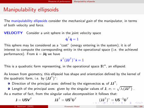
Measures of performance Manipulability ellipsoids
Manipulability ellipsoids
The manipulability ellipsoids consider the mechanical gain of the manipulator, in termsof both velocity and force.
VELOCITY Consider a unit sphere in the joint velocity space
qT q = 1
This sphere may be considered as a “cost” (energy entering in the system); it is ofinterest to compute the corresponding entity in the operational space (i.e. the achievedperformance). From x = Jq we have
xT (JJT )+x = 1
This is a quadratic form representing, in the operational space IRm, an ellipsoid.
As known from geometry, this ellipsoid has shape and orientation defined by the kernel ofthe quadratic form, i.e. by (JJT )+:
Direction of the principal axes: defined by the eigenvectos ui of JJT ;
Length of the principal axes: given by the singular values of J, σi =√
λi(JJT ) .
As a matter of fact, from the singular value decomposition it follows that:
J = USVT JJT = US2UT (JJT )+ = US−2UT
C. Melchiorri (DEIS) Kinematic Model 155 / 164
Measures of performance Manipulability ellipsoids
Manipulability ellipsoids
FORCE
Consider the mapping in the force/torque domain
τTτ = 1
from which (τ = JTw):wTJJTw = 1
This equation defines an ellipsoid in the operational force space IRm.
Similarly to the velocity case, we have that:
The principal axes of the ellipsoid are directed along the eigenvectors ui di JJT ;
Their length are proportional to the inverse of the singular values σi di J.
This is an important and remarkable result, that confirms the duality of the velocity andforce spaces:
The directions along which good performance are obtained in the velocity domain are
directions along which poor performance are obtained in the force domain, and viceversa
C. Melchiorri (DEIS) Kinematic Model 156 / 164
Measures of performance Manipulability ellipsoids
Manipulability ellipsoids
Some considerations:
Actuation needs a “large” gain; it is better along directions corresponding tolarge singular values;
Control: needs a “small” gain; it is better along directions whit smallersingular values (better sensitivity).
=⇒ The “optimal direction” for velocity (force) actuation is also the “optimaldirection” for controlling the force (velocity)
C. Melchiorri (DEIS) Kinematic Model 157 / 164
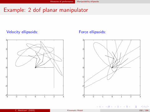
Measures of performance Manipulability ellipsoids
Example: 2 dof planar manipulator
Velocity ellipsoids:
-3 -2 -1 0 1 2 3-3
-2
-1
0
1
2
3
Force ellipsoids:
-3 -2 -1 0 1 2 3-3
-2
-1
0
1
2
3
C. Melchiorri (DEIS) Kinematic Model 158 / 164
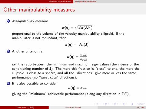
Measures of performance Manipulability ellipsoids
Other manipulability measures
1 Manipulability measure
w(q) =√
det(JJT )
proportional to the volume of the velocity manipulability ellipsoid. If themanipulator is not redundant, then
w(q) = |det(J)|
2 Another criterion is
w(q) =σmin
σmax
i.e. the ratio between the minimum and maximum eigenvalues (the inverse of theconditioning number of J). The more this fraction is “close” to one, the more theellipsoid is close to a sphere, and all the “directions” give more or less the sameperformance (no “worst case” directions).
3 It is also possible to considerw(q) = σmin
giving the “minimum” achievable performance (along any direction in IRm).
C. Melchiorri (DEIS) Kinematic Model 159 / 164
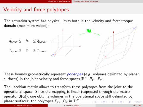
Measures of performance Velocity and force polytopes
Velocity and force polytopes
The actuation system has physical limits both in the velocity and force/torquedomain (maximum values):
qi ,min ≤ qi ≤ qi ,max
τi ,min ≤ τi ≤ τi ,max
These bounds geometrically represent polytopes (e.g. volumes delimited by planarsurfaces) in the joint velocity and force spaces IRn: Pq , Pτ .
The Jacobian matrix allows to transform these polytopes from the joint to theoperational space. Since the mapping is linear (expressed through the matrixoperator J(q)), one obtains volumes in the operational space still delimited byplanar surfaces: the polytopes Pv , Pw in IR
m.C. Melchiorri (DEIS) Kinematic Model 160 / 164
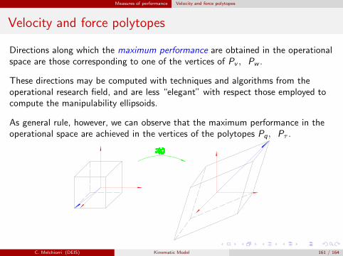
Measures of performance Velocity and force polytopes
Velocity and force polytopes
Directions along which the maximum performance are obtained in the operationalspace are those corresponding to one of the vertices of Pv , Pw .
These directions may be computed with techniques and algorithms from theoperational research field, and are less “elegant” with respect those employed tocompute the manipulability ellipsoids.
As general rule, however, we can observe that the maximum performance in theoperational space are achieved in the vertices of the polytopes Pq, Pτ .
C. Melchiorri (DEIS) Kinematic Model 161 / 164
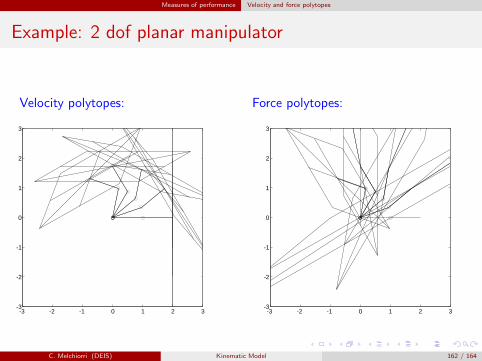
Measures of performance Velocity and force polytopes
Example: 2 dof planar manipulator
Velocity polytopes:
-3 -2 -1 0 1 2 3-3
-2
-1
0
1
2
3
Force polytopes:
-3 -2 -1 0 1 2 3-3
-2
-1
0
1
2
3
C. Melchiorri (DEIS) Kinematic Model 162 / 164
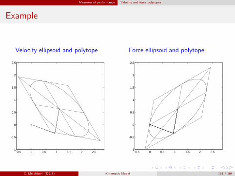
Measures of performance Velocity and force polytopes
Example
Velocity ellipsoid and polytope
-0.5 0 0.5 1 1.5 2 2.5-1
-0.5
0
0.5
1
1.5
2
2.5
Force ellipsoid and polytope
-0.5 0 0.5 1 1.5 2 2.5-1
-0.5
0
0.5
1
1.5
2
2.5
C. Melchiorri (DEIS) Kinematic Model 163 / 164
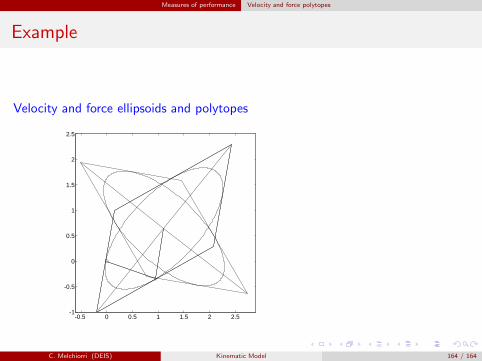
Measures of performance Velocity and force polytopes
Example
Velocity and force ellipsoids and polytopes
-0.5 0 0.5 1 1.5 2 2.5-1
-0.5
0
0.5
1
1.5
2
2.5
C. Melchiorri (DEIS) Kinematic Model 164 / 164


![arXiv:1711.03808v1 [cs.RO] 10 Nov 2017 · Servo Motor, PWM, Homogenous Transformations, Kinematic Chain, Denavit { Hartenberg Parameters, Schematic, Datasheet, Consumptions, Java-C++-C,](https://img.pdfslide.net/doc/110x75/5ec09c6fcb76bc13d41dde72/arxiv171103808v1-csro-10-nov-2017-servo-motor-pwm-homogenous-transformations.jpg)

![DYNAMICS CONTROL AND DH PARAMETRIZATION OF · PDF fileDenavit-Hartenberg notation (Fig.1) is widely used in the transformation of coordinate systems of linkages and robot mechanisms[1]](https://img.pdfslide.net/doc/110x75/5a8794817f8b9a882e8dbf44/dynamics-control-and-dh-parametrization-of-notation-fig1-is-widely-used-in.jpg)


![AUTOMATED NON-DESTRUCTIVE EXAMINATION OF … · (Denavit–Hartenberg) kinematic coefficients for the robot and additional degrees of freedom [Ref 4] Figure 4: Typical robotic NDE](https://img.pdfslide.net/doc/110x75/5bdf515f09d3f251108b56df/automated-non-destructive-examination-of-denavithartenberg-kinematic-coefficients.jpg)