Lab 5 Filtersrfic.eecs.berkeley.edu/ee100/labs/lab5.pdf · and$disadvantages.$ Pre$Lab)Component) Background)and)Theory) Asyou$may$recall,$each$passive$circuit$component$(resistor,$inductor,$and$capacitor)$can$be$abstracted$

Lab 5: Filters EE43/100 Spring 2012 V. Lee, T. Dear, T. Takahashi

1

Filters LAB 5: Filters

ELECTRICAL ENGINEERING 43/100

INTRODUCTION TO DIGITAL ELECTRONICS

University Of California, Berkeley

Department of Electrical Engineering and Computer Sciences

Professor Ali Niknejad, Professor Michel Maharbitz,

Vincent Lee, Tony Dear, Toshitake Takahashi

Lab Contents:

I. Lab Objectives II. Pre-‐Lab Component

a. Background and Theory b. Voltage Dividers and Filters

III. Lab Component a. Passive Low-‐Pass Filters b. Passive High-‐Pass Filters c. Active Filters

IV. Lab Submissions a. Image Citations

YOUR NAME: YOUR SID:

YOUR PARTNER’S NAME: YOUR PARTNER’S SID:

Pre-‐Lab: __/10 Lab: __/90

Total: ___/100


2

Lab Objectives

Filters have a wide range of applications and can be found in many electronic devices. Such applications include a low-‐pass filter in your telephone landline, a high-‐pass filter for your high-‐bandwidth DSL modem, a band-‐pass filter in your cell phone so that you only hear the person you’re speaking with and not everyone else on their phones around you, a band-‐reject filter to reject the 50 Hz or 60 Hz AC power signal when using sensitive components, and many other applications in audio processing, communications, sensors, etc.

In this lab we will be implementing both passive and active filters, each of which have their advantages and disadvantages.

Pre-‐Lab Component

Background and Theory

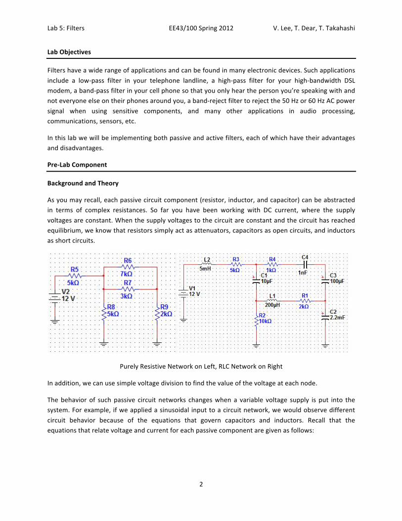
As you may recall, each passive circuit component (resistor, inductor, and capacitor) can be abstracted in terms of complex resistances. So far you have been working with DC current, where the supply voltages are constant. When the supply voltages to the circuit are constant and the circuit has reached equilibrium, we know that resistors simply act as attenuators, capacitors as open circuits, and inductors as short circuits.

Purely Resistive Network on Left, RLC Network on Right

In addition, we can use simple voltage division to find the value of the voltage at each node.

The behavior of such passive circuit networks changes when a variable voltage supply is put into the system. For example, if we applied a sinusoidal input to a circuit network, we would observe different circuit behavior because of the equations that govern capacitors and inductors. Recall that the equations that relate voltage and current for each passive component are given as follows:


3

Resistor 𝑉 = 𝐼𝑅

Capacitor

𝐼 = 𝐶𝑑𝑉𝑑𝑡

Inductor

𝑉 = 𝐿𝑑𝐼𝑑𝑡

So for constant voltages such that 𝑉 = 𝑉!, we obtain:

Resistor

𝐼 =𝑉!𝑅

Capacitor

𝐼 = 𝐶𝑑𝑑𝑡𝑉! = 0

Inductor

𝐼 =𝑉!𝐿𝑑𝑡 + 𝐼!"!#

And for constant current such that 𝐼 = 𝐼! we obtain:

Resistor 𝑉 = 𝐼!𝑅

Capacitor

𝑉 =𝐼!𝐶𝑑𝑡 + 𝑉!"!#

Inductor

𝑉 = 𝐿𝑑𝑑𝑡𝐼! = 0

Now let’s consider what happens when we apply a sinusoidal input. Suppose the input signal is given by 𝑉 𝑡 = 𝑉!sin (𝜔𝑡); what is the resulting current?

Resistor

𝐼 𝑡 =𝑉!sin (𝜔𝑡)

𝑅

Capacitor

𝐼 𝑡 = 𝐶𝑑𝑑𝑡𝑉! sin 𝜔𝑡= 𝜔𝐶𝑉! cos 𝜔𝑡

Inductor 𝐼 𝑡 =

𝑉! sin 𝜔𝑡𝐿

𝑑𝑡 = −𝑉!cos (𝜔𝑡)

𝜔𝐿

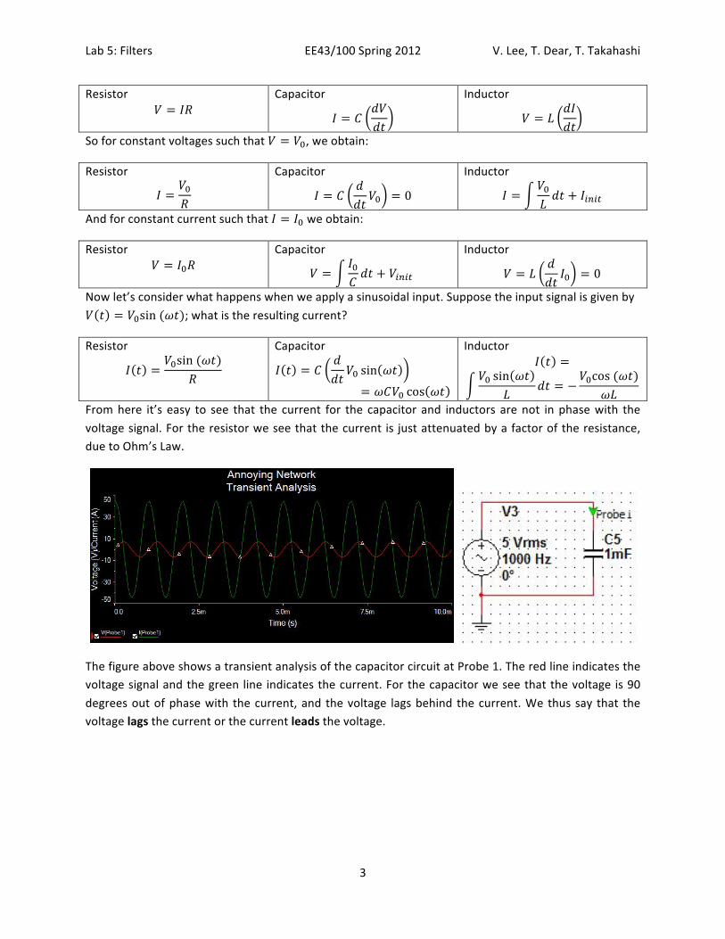
From here it’s easy to see that the current for the capacitor and inductors are not in phase with the voltage signal. For the resistor we see that the current is just attenuated by a factor of the resistance, due to Ohm’s Law.

The figure above shows a transient analysis of the capacitor circuit at Probe 1. The red line indicates the voltage signal and the green line indicates the current. For the capacitor we see that the voltage is 90 degrees out of phase with the current, and the voltage lags behind the current. We thus say that the voltage lags the current or the current leads the voltage.


4

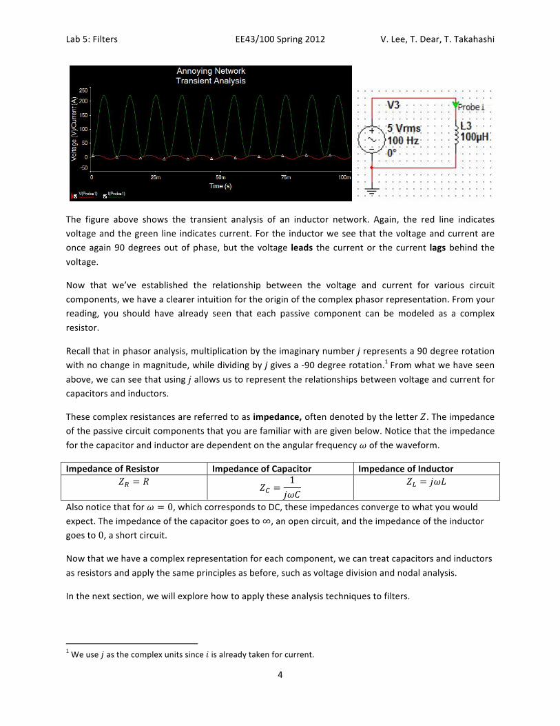
The figure above shows the transient analysis of an inductor network. Again, the red line indicates voltage and the green line indicates current. For the inductor we see that the voltage and current are once again 90 degrees out of phase, but the voltage leads the current or the current lags behind the voltage.

Now that we’ve established the relationship between the voltage and current for various circuit components, we have a clearer intuition for the origin of the complex phasor representation. From your reading, you should have already seen that each passive component can be modeled as a complex resistor.

Recall that in phasor analysis, multiplication by the imaginary number 𝑗 represents a 90 degree rotation with no change in magnitude, while dividing by 𝑗 gives a -‐90 degree rotation.1 From what we have seen above, we can see that using 𝑗 allows us to represent the relationships between voltage and current for capacitors and inductors.

These complex resistances are referred to as impedance, often denoted by the letter 𝑍. The impedance of the passive circuit components that you are familiar with are given below. Notice that the impedance for the capacitor and inductor are dependent on the angular frequency 𝜔 of the waveform.

Impedance of Resistor Impedance of Capacitor Impedance of Inductor 𝑍! = 𝑅 𝑍! =

1𝑗𝜔𝐶

𝑍! = 𝑗𝜔𝐿

Also notice that for 𝜔 = 0, which corresponds to DC, these impedances converge to what you would expect. The impedance of the capacitor goes to ∞, an open circuit, and the impedance of the inductor goes to 0, a short circuit.

Now that we have a complex representation for each component, we can treat capacitors and inductors as resistors and apply the same principles as before, such as voltage division and nodal analysis.

In the next section, we will explore how to apply these analysis techniques to filters.

1 We use 𝑗 as the complex units since 𝑖 is already taken for current.


5

Voltage Dividers and Filters

Now that we’ve established how to break down complicated passive circuit networks into a network of complex resistors, we can simply apply the basic principles pertaining to resistive networks as we did in lab 2. Techniques such as voltage divider and node voltage analysis still apply to resistive networks with complex resistors or impedances.

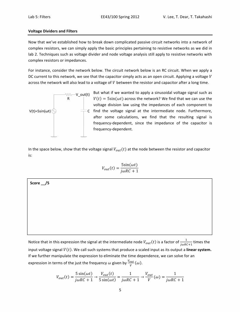
For instance, consider the network below. The circuit network below is an RC circuit. When we apply a DC current to this network, we see that the capacitor simply acts as an open circuit. Applying a voltage 𝑉 across the network will also lead to a voltage of 𝑉 between the resistor and capacitor after a long time.

But what if we wanted to apply a sinusoidal voltage signal such as 𝑉 𝑡 = 5sin(𝜔𝑡) across the network? We find that we can use the voltage division law using the impedances of each component to find the voltage signal at the intermediate node. Furthermore, after some calculations, we find that the resulting signal is frequency-‐dependent, since the impedance of the capacitor is frequency-‐dependent.

In the space below, show that the voltage signal 𝑉!"#(𝑡) at the node between the resistor and capacitor is:

𝑉!"# 𝑡 =5sin(𝜔𝑡)𝑗𝜔𝑅𝐶 + 1

Notice that in this expression the signal at the intermediate node 𝑉!"# 𝑡 is a factor of !!"#$!!

times the

input voltage signal 𝑉 𝑡 . We call such systems that produce a scaled input as its output a linear system. If we further manipulate the expression to eliminate the time dependence, we can solve for an

expression in terms of the just the frequency 𝜔 given by !!"#!

𝜔 .

𝑉!"# 𝑡 =5 sin 𝜔𝑡𝑗𝜔𝑅𝐶 + 1

→𝑉!"# 𝑡5 sin 𝜔𝑡

=1

𝑗𝜔𝑅𝐶 + 1→𝑉!"#𝑉

(𝜔) =1

𝑗𝜔𝑅𝐶 + 1

Score __/5


6

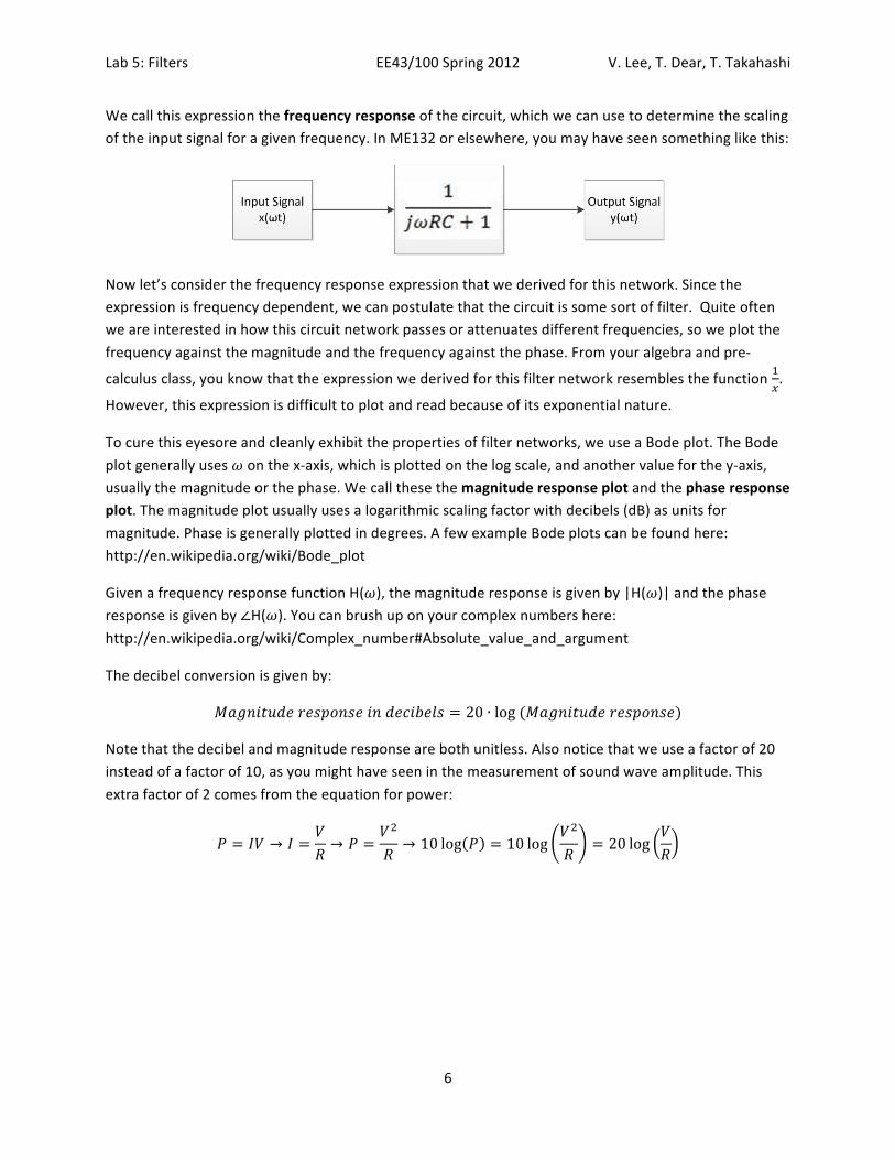
We call this expression the frequency response of the circuit, which we can use to determine the scaling of the input signal for a given frequency. In ME132 or elsewhere, you may have seen something like this:

Now let’s consider the frequency response expression that we derived for this network. Since the expression is frequency dependent, we can postulate that the circuit is some sort of filter. Quite often we are interested in how this circuit network passes or attenuates different frequencies, so we plot the frequency against the magnitude and the frequency against the phase. From your algebra and pre-‐

calculus class, you know that the expression we derived for this filter network resembles the function !!.

However, this expression is difficult to plot and read because of its exponential nature.

To cure this eyesore and cleanly exhibit the properties of filter networks, we use a Bode plot. The Bode plot generally uses 𝜔 on the x-‐axis, which is plotted on the log scale, and another value for the y-‐axis, usually the magnitude or the phase. We call these the magnitude response plot and the phase response plot. The magnitude plot usually uses a logarithmic scaling factor with decibels (dB) as units for magnitude. Phase is generally plotted in degrees. A few example Bode plots can be found here: http://en.wikipedia.org/wiki/Bode_plot

Given a frequency response function H(𝜔), the magnitude response is given by |H(𝜔)| and the phase response is given by ∠H(𝜔). You can brush up on your complex numbers here: http://en.wikipedia.org/wiki/Complex_number#Absolute_value_and_argument

The decibel conversion is given by:

𝑀𝑎𝑔𝑛𝑖𝑡𝑢𝑑𝑒 𝑟𝑒𝑠𝑝𝑜𝑛𝑠𝑒 𝑖𝑛 𝑑𝑒𝑐𝑖𝑏𝑒𝑙𝑠 = 20 ∙ log (𝑀𝑎𝑔𝑛𝑖𝑡𝑢𝑑𝑒 𝑟𝑒𝑠𝑝𝑜𝑛𝑠𝑒)

Note that the decibel and magnitude response are both unitless. Also notice that we use a factor of 20 instead of a factor of 10, as you might have seen in the measurement of sound wave amplitude. This extra factor of 2 comes from the equation for power:

𝑃 = 𝐼𝑉 → 𝐼 =𝑉𝑅→ 𝑃 =

𝑉!

𝑅→ 10 log 𝑃 = 10 log

𝑉!

𝑅= 20 log

𝑉𝑅


7

Using the decibel conversion given above, and the expression we derived for !!"#!(𝜔), draw the Bode

plot (both magnitude and phase) in the space provide below. Clearly label your axes and increments and indicate any relevant points on the graph in terms of the variables 𝑉!"# ,𝑉,𝜔,𝑅, and 𝐶.

For your Bode plot, you should have found that the circuit network attenuates higher frequencies at a rate of 20 dB per decade. Such circuit systems that pass lower frequencies are known as low pass filters (LPF).

You will notice on the Bode plot that there is an initial plateau before the frequency 𝜔 = !!", followed by

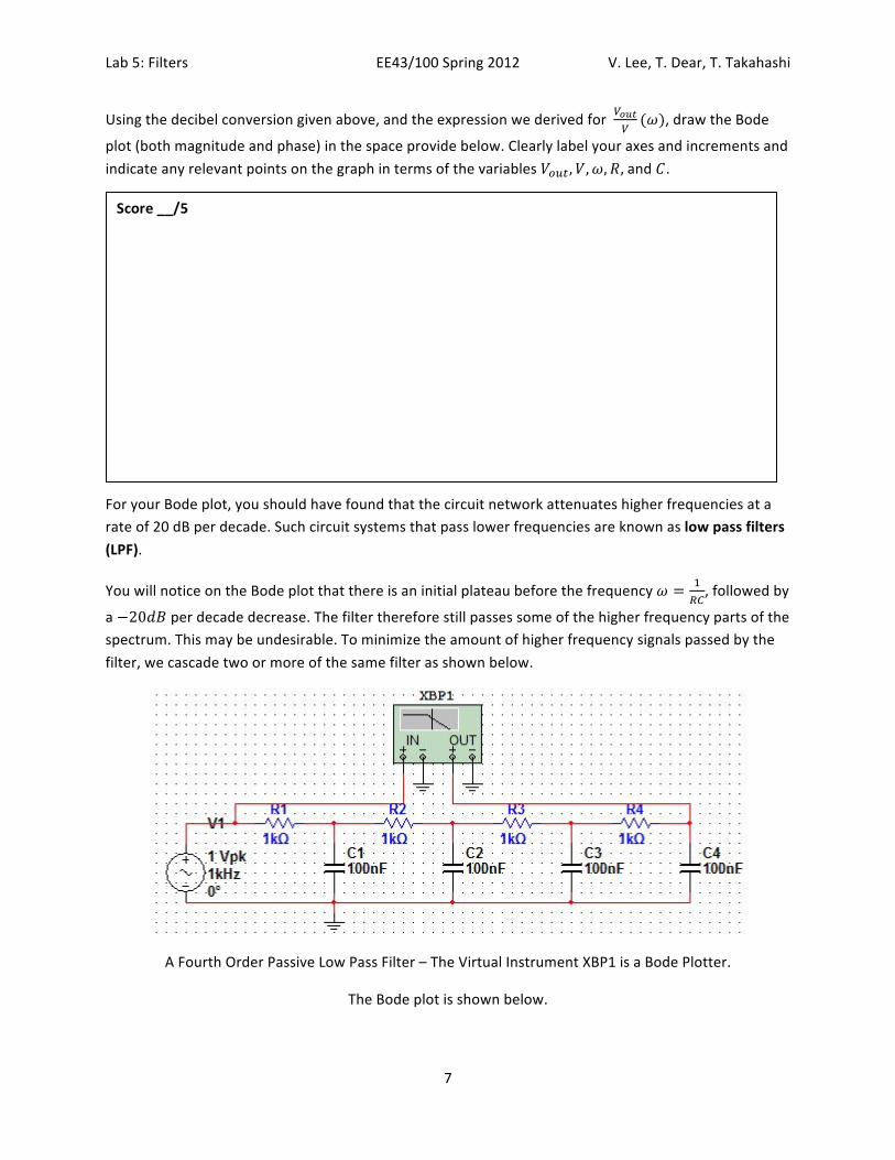
a −20𝑑𝐵 per decade decrease. The filter therefore still passes some of the higher frequency parts of the spectrum. This may be undesirable. To minimize the amount of higher frequency signals passed by the filter, we cascade two or more of the same filter as shown below.

A Fourth Order Passive Low Pass Filter – The Virtual Instrument XBP1 is a Bode Plotter.

The Bode plot is shown below.

Score __/5


8

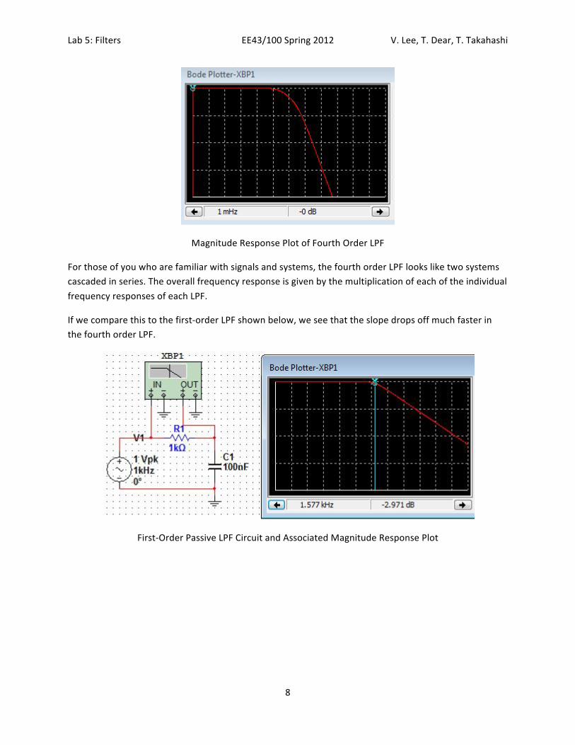
Magnitude Response Plot of Fourth Order LPF

For those of you who are familiar with signals and systems, the fourth order LPF looks like two systems cascaded in series. The overall frequency response is given by the multiplication of each of the individual frequency responses of each LPF.

If we compare this to the first-‐order LPF shown below, we see that the slope drops off much faster in the fourth order LPF.

First-‐Order Passive LPF Circuit and Associated Magnitude Response Plot


9

Lab Component

A common application of filters is to eliminate undesired frequencies such as high-‐frequency noise or low-‐frequency DC components. In music applications, we may want to extract certain frequency bands, boost bass, or keep only high frequencies for various audio processing techniques.

The most common filters that you will encounter are the low-‐pass, high-‐pass, band-‐pass, and band-‐reject filters. Many other filters also exist, but the mathematical analysis required to design those filters is out of the scope of this course (see EE120). As was discussed earlier, these filters can also be active or passive.

In the first part of the lab, we will start with the passive filters. Later we move onto active filters. In particular, we want to pay attention to the low-‐pass filters.

Passive Low-‐Pass Filters

In audio applications, it is important to eliminate any stray high-‐frequency content which can potentially damage your hearing. Thus, it is common practice to liberally apply low-‐pass filters to kill these undesired frequencies. So how do we do that?

We know that the audible hearing range spans from about 20 Hz to 20000 Hz, so we’ll start with that. In the space provided below or a separate sheet of paper, design a passive low pass filter such that the cutoff frequency will adequately attenuate the high frequencies and pass the low frequencies. Explain all calculations and draw the Bode plot (both magnitude and phase) for your filter. Hint: Remember 𝜔 has units of rad/s, f has units of Hz, and 𝜔 = 2π𝑓.

Score __/15


10

Now that we have our low-‐pass filter, we will see if it works. Before we apply the corrupted signal, we will test our filter using the function generator.

For starters, first build your circuit and make sure to note where the input voltage signal and the output voltage signal should be.

Turn on your function generator and make sure that it is a sinusoidal waveform. You may also want to set the peak-‐to-‐peak voltage to something like 5𝑉.

Connect the function generator to the input of the filter and ground.

Now turn on your oscilloscope. We will be using this to observe the attenuation of the input waveform by comparing it to the output waveform.

Connect one scope to the input of the filter and measure the peak-‐to-‐peak value of the input waveform.

Connect the other scope to the output of the filter and measure the peak-‐to-‐peak value of the output waveform.

At this point, your set up should show two waveforms on the oscilloscope of the same frequency (try auto-‐scaling if you don’t). You should also have two peak-‐to-‐peak measurements active on your oscilloscope. If you don’t, make sure to hit Voltage and V-‐pp to get the peak-‐to-‐peak measurements.

More workspace…


11

We can now verify if our filter is working properly. To do this, let’s change the frequency of the input waveform by adjusting the function generator. By doing this, we can sweep a range of frequencies, check the attenuation, and verify if it matches our Bode plot.

Take your function generator and set the frequency to 1 Hz. (This is essentially a constant signal).

Check the peak-‐to-‐peak value of the input and the peak-‐to-‐peak value of the output.

Calculate the attenuation (or amplification) and verify that it matches your predict value on your Bode plot.

Repeat this at 10 x increments (i.e., increase the frequency ten times for each measurement). Record your measurements in the table provided below. If your values tend to deviate too far from predicted values, you may want to verify your calculations. (5 pts)

Frequency Peak-‐to-‐peak value of input

Peak-‐to-‐peak value of output

Gain/Attenuation Factor

Gain/Attenuation in dB

1 Hz 10 Hz 100 Hz 1 kHZ 10 kHz 100 kHz 1 MHz 10 MHz

Passive High Pass Filters

Now suppose we wanted a passive high-‐pass filter that rejected frequencies below 1000𝐻𝑧. In the space provided below, design a passive HPF and prove that it adequately rejects frequencies below the cutoff frequency. Also explain all calculations and provide a Bode plot (both magnitude and phase).

Score: __/10


12

Now suppose you put your low pass filter with the high pass filter together (i.e., the output of the low pass filter is the input to the high pass filter). Neglecting any interaction between the filters, what type of filter do you get? (You don’t actually have to do this.) If we hacked a microphone with this filter, do you think a man or a woman would be more understandable when speaking through the mic?

Active Filters

In the previous parts, we have been using what we call passive components (resistors, capacitors, and inductors) to implement our filters. We call these filters passive because they do not require a power source to operate. Consequently, these filters can only pass or attenuate the input signals, and may require a separate amplification stage.

An alternative to passive filters are active filters. Typically, an active filter will use one or more operational amplifiers to amplify the signal and filter it at the same time.

There are many different ways to implement an active LPF, but all active filters, as the name implies, use an active circuit element like an op amp. For this portion of the lab, we will supply you with the necessary circuit. It will be your job to figure out how it works.

Note that the maximum gain of this circuit is not limited to 1 unlike passive filters.

Below is the circuit schematic for an active low pass filter:

More workspace…

Score: __/5


13

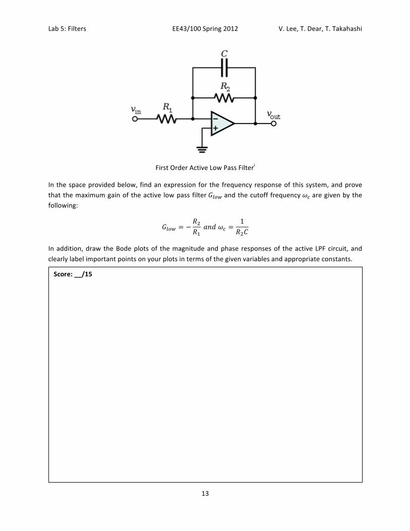
First Order Active Low Pass Filteri

In the space provided below, find an expression for the frequency response of this system, and prove that the maximum gain of the active low pass filter 𝐺!"# and the cutoff frequency 𝜔! are given by the following:

𝐺!"# = −𝑅!𝑅! 𝑎𝑛𝑑 𝜔! =

1𝑅!𝐶

In addition, draw the Bode plots of the magnitude and phase responses of the active LPF circuit, and clearly label important points on your plots in terms of the given variables and appropriate constants.

Score: __/15


14

Now that you have a better idea of what’s going on, choose components values such that the cutoff frequency for your active low-‐pass filter is 100𝐻𝑧 and the maximum gain is approximately 10. Then implement your filter and fill out the following measurements as you did with the passive filters in the previous parts. (5 pts)

Frequency Peak-‐to-‐peak value of input

Peak-‐to-‐peak value of output

Gain/Attenuation Factor

Gain/Attenuation in dB

1 Hz 10 Hz 100 Hz 1 kHZ 10 kHz 100 kHz 1 MHz 10 MHz

Show your active filter set up to your GSI for check off. Make sure you are able to demonstrate and explain why your filter works using your scope.

Your GSI Signs Here (35 pts)

More workspace…


15

Lab Report Submissions

This lab is due at the beginning of the next lab section. Make sure you have completed all questions and drawn all the diagrams for this lab. In addition, attach any loose papers specified by the lab and submit them with this document.

These labs are designed to be completed in groups of two. Only one person in your team is required to submit the lab report. Make sure the names and student IDs of BOTH team members are on this document (preferably on the front).

Image Citations

i http://upload.wikimedia.org/wikipedia/commons/5/59/Active_Lowpass_Filter_RC.svg

Documents

Lab 5 Filtersrfic.eecs.berkeley.edu/ee100/labs/lab5.pdf · and$disadvantages.$ Pre$Lab)Component) Background)and)Theory) Asyou$may$recall,$each$passive$circuit$component$(resistor,$inductor,$and$capacitor)$can$be$abstracted$