Embed Size (px)
Citation preview

GNSS Data Processing
Laboratory
Slides
gA
GE
rese
arc
h g
rou
p o
f A
str
on
om
y a
nd
gAGE
Geo
mati
cs
http://www.gage.upc.edu
@ J. Sanz Subirana & J.M. Juan Zornoza
Barc
elo
na,
Spain

Authorship statement
The authorship of this material and the Intellectual Property Rights are owned
by J. Sanz Subirana and J.M. Juan Zornoza.
These slides can be obtained either from the server http://www.gage.upc.edu,
or [email protected]. Any partial reproduction should be previously
authorized by the authors, clearly referring to the slides used.
This authorship statement must be kept intact and unchanged at all times.
5 March 2017
Contents
Tutorial 0: UNIX environment, tools and skills. GNSS standard files formats.
Tutorial 1: GNSS data processing laboratory exercises.
Tutorial 2: Measurements analysis and error budget.
Tutorial 3: Differential positioning with code measurements.
Tutorial 4: Carrier ambiguity fixing.
Tutorial 5: Analysis of propagation effects from GNSS observables based on laboratory exercises.
Tutorial 6: Differential positioning and carrier ambiguity fixing.
List of Acronyms.

Tutorial 0UNIX enviroment, Tools and Skills.
GNSS Standard File Formats
J. Sanz Subirana and J.M. Juan Zornoza
November 27, 2013

Tutorial 0.1. UNIX Environment, Tools and Skills
Tutorial 0.1. UNIX Environment, Tools and Skills
Objectives
To present a (very limited) set of UNIX instructions in order tomanage files and directories, as well as some basic elements ofawk/gawk programming and the graphical plotting environmentgraph.py. The aim is not to teach UNIX or programming lan-guages, but to provide some basic tools needed to develop thepractical sessions.
Note: The following exercises are very elementary and can beomitted if the reader already has some basic knowledge of UNIXand gawk.
Files to usesxyz.eci
Programs to usegraph.py
Development
This session has been organised as a series of guided exercises to be done inthe established order, which introduces the main instructions for use in thefollowing sessions.
1. First instructions
(a) Show the name of the directory where you are located.Execute: pwd
(b) Examine the directory content.Execute: ls -lt
(c) Go to the personal directory or home directory (‘∼’).Execute: cd or cd ∼
(d) Go to the GNSS directory (inside the home directory)1
Execute: cd GNSS
(e) Access the HTML directory and view its contents.Execute:
cd HTML
ls -lt
(f) Go back to the home directory.Execute: cd ∼
1If the installation has been done properly according to instructions in the installationguide, the following three directories will be found: FILES, PROG and HTML. These directories,together with the Notepad files, will appear in the home/GNSS directory.
1
gAGE/UPC
(g) Show a text line on the screen:Execute:echo "Have a nice day"
(h) Direct the contents to a file:Execute:
echo "Have a nice day" > test
ls -ltr
echo "you too" >> test
(i) Show the contents of the file on the screen:Execute:cat test
Try to execute this too: echo test. What happens?
(j) Edit a fileExecute:2
textedit test
2. Directory management
(a) From any directory where you are located, go to the GNSS directoryand check that you are in it. Create the directory working insidethe GNSS directory. Access it. Go back to the directory immediatelyabove (in this case the GNSS directory) by executing ‘..’).Execute:
cd ∼/GNSSpwd
mkdir working
cd working
pwd
cd ..
pwd
3. File management
(a) Go to the working directory (which is inside the GNSS directory).Copy the file test from the home directory (‘∼’) to your currentdirectory (symbolised by ‘.’).Execute:
cd ∼/GNSS/workingcp ∼/test .
ls -lt
(b) Copy the file test to the file file1.3 Check the contents of file1.Execute:
cp test file1
ls -lt
more file1
2Any text editor can also be used.3As file file1 does not exist, a new file will be created with this name and with the
same contents as file test.
2
Tutorial 0.1. UNIX Environment, Tools and Skills
(c) Create a ‘link’4 from file file2 to file test. Check the file contents.Check the contents of file2.Execute:
ln -s test file2
ls -lt
more file2
(d) Using a text editor (e.g. gedit or similar), edit file2 and change theword day to the word YEAR. Save the changes and exit gedit. Next,check the contents of file test and its link file2. Have the contentsof the original file test been modified through its link file2?Execute:
gedit file2
more test
more file1
(e) Remove file file1 and its link file2. Check if they have beendeleted. Create the directory other. Remove the directory other.Execute:
ls -lt
rm file1 file2
ls -lt
mkdir other
ls -lt
rm -r other
ls -lt
(f) Find information on the ‘mkdir’ and ‘rm’ commands in the help pages(i.e. in the UNIX manual).Execute:
man mkdir
man rm
4. Programming environment gawk5
(a) From within the working directory, create a link from file sxyz.eci
(which is placed in the directory GNSS/FILES/TUT0) to a file withthe same name in the working directory.Execute:
cd ∼/GNSS/workingln -s ∼/GNSS/FILES/TUT0/sxyz.eci .
ls -lt
The file sxyz.eci contains three columns of coordinates, in a geo-centric inertial system, of a set of satellites at different epochs. Itcontains the following fields:
SATELLITE time(sec) X(km) Y(km) Z(km)
4This differs from the previous case because file2 is not a new file, just a pointer tofile test. Thus, the ‘link’ file2 represents the minimum space expense, independent ofthe file test size. Execute man ln to see the meaning of different types of links.
5gawk is the GNU implementation of awk (from the Free Software Foundation).
3
gAGE/UPC
(b) Execute the instructions cat, more and less in order to display thefile contents sxyz.eci. What differences can be seen among theseinstructions?6
Execute:
cat sxyz.eci
more sxyz.eci
less sxyz.eci
cat sxyz.eci | less
(c) Using the programming language gawk, print (on screen) the firstand third fields of file sxyz.eci.Execute:
gawk ’{print $1,$3}’ sxyz.eci |more
or
cat sxyz.eci |gawk ’{print $1,$3}’ |more
(d) Now print all the fields at the same time.Execute:
cat sxyz.eci | gawk ’{print $0}’ | more
(e) The following instruction generates the file prb1 which contains datafrom a single satellite. Which satellite is selected?Execute:
cat sxyz.eci | gawk ’{if ($1==5) print $0 }’ > prb1
more prb1
(f) What is the meaning of the values in the second column of file prb2
generated by the next instruction?Execute (in a single line):7
cat sxyz.eci | gawk ’{if ($1==5)
print $2,sqrt($3**2+$4**2+$5**2)}’> prb2
more prb2
(g) Discuss the structure of the following instruction that makes a ‘print’with a particular format (where %i=integer, %f= float, %s= string).Execute:
cat sxyz.eci |gawk ’{printf"%2i %02i %11.3f %i %s \n",$1,$1,$3,$3, $1}’|more
(h) Access the manual pages of gawk.Execute:
man gawk
6The command ‘|’ allows us to connect the output of a process with the input of another.For example, the output of cat can be sent to more.
7The sentence line is a single line, although it may appear as two lines because oftypesetting constraints.
4
Tutorial 0.1. UNIX Environment, Tools and Skills
5. Graphics environment graph.py
(a) Program graph.py is in directory∼/GNSS/PROG/src/gLAB src. Linkthis program to the current directory "." (i.e. directory working).Execute:
ln -s ∼/GNSS/PROG/src/gLAB src/graph.py .
(b) For the previously generated file prb1, plot the third field (x coordi-nate) as a function of the second one (time in seconds).Execute:8
graph.py -f prb1 -x2 -y3
(c) Using file sxyz.eci, plot satellites #5 and #9.Execute:9
graph.py -f sxyz.eci -x2 -y3 -c ’($1 == 5)’
-f sxyz.eci -x2 -y3 -c ’($1 == 9)’
(d) Repeat the previous plot for the interval [20 000 : 30 000] on the x-axis.Execute:
graph.py -f sxyz.eci -x2 -y3 -c ’($1 == 5)’
-f sxyz.eci -x2 -y3 -c ’($1 == 9)’
--xn 20000 --xx 30000
(e) Using file prb1, plot on the same graph the x (third field), y (fourthfield) and z (fifth field) coordinate as a function of time (second field).Execute:
graph.py -f prb1 -x2 -y3 -f prb1 -x2 -y4 -f prb1 -x2 -y5
(f) Using file prb1, plot on the same graph the distance of the satellitesfrom Earth’s mass centre (r =
√x2 + y2 + z2) as a function of time.
Execute:
graph.py -f prb1 -x2 -y’math.sqrt($3*$3+$4*$4+$5*$5)’
(g) For the same file used in the previous cases (prb1), write the title"orbit", x label "sec" and y label "m".Execute:
graph.py -f prb1 -x2 -y3 -t "orbit" --xl "sec" --yl "m"
8Depending on the PATH configuration, it would be necessary to execute ‘./graph.py’instead of ‘graph.py’. Another possibility is to include the current directory ‘.’ in the PATH
variable of the current terminal. This is done in the bash environment by executing export
PATH="./:$PATH". On the other hand, if we want to make this PATH update permanent,then the sentence export PATH="./:$PATH" must be included at the end of file ‘.bashrc’in the home directory. When working in tcsh instead of bash, the equivalent sentences areas follows: execute set PATH=./:${PATH} in the current directory (for a non-permanentchange), or add the sentence set path=(./ $path) to the end of file /etc/csh.cshrc tomake the PATH update permanent. Note that, in this last case, administrator privileges areneeded to edit the /etc/csh.cshrc file.
9Note that, in the Windows OS, instructions like ’($1=="5")’ must be written as"($1==’5’)"; that is, replacing (") by (’).
5
gAGE/UPC
(h) Visualise the different forms of graphic representations in the follow-ing instructions (with points, lines and other symbols or colours).
Execute:
graph.py -f prb1 -x2 -y3 -s.
graph.py -f prb1 -x2 -y3 -s-
graph.py -f prb1 -x2 -y3 -s-.
graph.py -f prb1 -x2 -y3 -s--
graph.py -f prb1 -x2 -y3 -so
graph.py -f prb1 -x2 -y3 -s+
graph.py -f prb1 -x2 -y3 -sp
graph.py -f prb1 -x2 -y3 -so --cl r
graph.py -f prb1 -x2 -y3 -s. --cl g
(i) Save the plot in a POSTSCRIPT file "orbit.ps" and in a PNG! (PNG!)
file "orbit.png".Execute:
graph.py -f prb1 -x2 -y3 --sv orbit.ps
graph.py -f prb1 -x2 -y3 --sv orbit.png
(j) Check "help" in graph.py.Execute:
graph.py -help
6
Tutorial 0.2. GNSS Standard File Format
Tutorial 0.2. GNSS Standard File Format
By Adria Rovira Garcıa
gAGE/UPC & gAGE-NAV, S.L.
Objectives
To become familiar with the different format standard(s) involvedin the GNSS data sets. To provide the user with a reliable andpowerful tool to learn the standard formats in a very easy andfriendly way, aided by explanatory tool tips. These tips will betriggered automatically when the mouse is hovered over a field.The explanations include a description of the field, the format inwhich it is written and, if applicable, its units.
Files to useLaunchHTML.html, GLONASS Navigation Rinex v2.11.html,SP3 Version C.html, Observation Rinex v3.01.html,ANTEX v1.3.html, Observation Rinex v2.11.html,IONEX v1.0.html, Observation Rinex v2.10.html,SP3 Version C.html, RINEX CLOCKS v3.00.html,SBAS Navigation Rinex v3.01.html,GPS Navigation Rinex v2.11.html
Programs to useAny Web browser (Firefox can be used, as well).
Development
1. RINEX measurement files: v2.10
This standard gathers the GNSS observations collected by a receiver. Thefile is divided clearly into two different sections: the header section andthe observables section. While in the header global information is givenfor the entire file, the observables section contains the code and carriermeasurements, among others, stored by epoch.
Open file Observation Rinex v2.10.html with a Web browser and an-swer the following questions (the answer is provided at the end of eachquestion).
(a) Hover the mouse over the title ‘Observation RINEX 2.10 Format’,where some general information is given. Which was the first insti-tution to develop this format?
→ The Astronomical Institute of the University of Berne.
(b) What was the reason for developing such a standard?
→ The exchange of GPS data from several different GPS receivers.
7
gAGE/UPC
(c) Which type of optimisation has been applied to this standard?
→ Minimum space requirements, keeping the observation records as shortas possible.
(d) What is the maximum record (i.e. line) length?
→ Files are kept to 81-character lines.
(e) The header section contains a set of labels. Where are they located?
→ The header labels are located between the 61st and the 80st columnof each line.
(f) Where can a collection of currently used formats be found?
→ On the IGS website:http://igscb.jpl.nasa.gov/components/formats.html .
(g) The header section of this file is dual coloured in order to distinguishheader information from header labels. What is the first and the lastheader label of the header section?
→ The first label is ‘RINEX VERSION / TYPE’ while the last label is ‘ENDOF HEADER’.
(h) What is the difference between the ‘RINEX VERSION / TYPE’ and the‘COMMENT ’ labels?
→ While the first one is a mandatory label, the second is optional andmay not appear in some RINEX files.
(i) Hover over the first field in the ‘RINEX VERSION / TYPE’ line; whatis the main advance in this RINEX version?
→ Version 2 has been prepared to contain GLONASS or other satellitesystem observations apart from GPS satellites.
(j) Where is the antenna located approximately? In which referencesystem?
→ The approximate antenna position is (478 902 8.4701, 176 610.0133,419 501 7.0310) in the WGS-84 system.
(k) Hover over the first field in the ‘LEAP SECONDS’ line; what is thedifference between the various satellite systems, when counting leapseconds?
→ The Glonass time system is tied to UTC, so leap seconds are needed,for instance, to mix Galileo or GPS with Glonass data.
(l) How many satellites are present in the current file? To which satellitesystem do they belong?
→ There are 14 different satellites:14 GNSS satellites = 10 GPS + 3 Glonass + 1 SBAS.
8
Tutorial 0.2. GNSS Standard File Format
(m) Line ‘PRN / # OF OBS ’ has to be consistent with the observableslisted in line ‘# / TYPES OF OBSERV’. What are these observations?Do all satellites contain the same observables in this example?
→ The observables are: L1, L2, P1, P2, C1, S1, S2.Glonass and SBAS satellites only have: L1, C1, S1.
(n) How does the standard indicate the end of the header?
→ The last field of the header is a record of 60 empty characters.
(o) The data section of this file is again dual coloured in order to distin-guish blocks of data. According two the different colours used, howmany epochs are included in this file?
→ There are two different epochs, each with a different colour.
(p) The first line of an epoch contains information on a whole block ofmeasurements. When is the first epoch of the file?
→ The first epoch corresponds to 5/3/2010 at 00:00:00.
(q) How many satellites are present in the first epoch? Is there anyparticular feature occurring due to this number?
→ The first epoch contains 14 different satellites. Because there aremore than 12 satellites, the list of epoch satellites is divided into twodifferent lines.
(r) Measurements follow the order stated in line ‘# / TYPES OF OBSERV’line. The satellite order is given in the first line of the epoch. Whatare the units for the observables?
→ L1, L2: cycles of the carrier.P1, P2, C1: metres.S1, S2: receiver dependent.
(s) Hover over the first L1 measure of satellite G13. The measure is giventogether with two indicators. What are these indicators? What dothey represent?
→ Loss of Lock Indicator: Depending on its value, it can show a cycleslip, an opposite wavelength factor, or an anti-spoofing measurement.Signal Strength: Projected into the [1-9] interval.
2. RINEX measurement files: v2.11
Open file Observation Rinex v2.11.html with a Web browser.
(a) Hover over the ‘WAVELENGTH FACT L1/2’ line records. The first linestates the default values for the wavelength measures for the L1and L2 frequencies. Which satellite system do the default valuesapply to? Interpret the second line of the ‘WAVELENGTH FACT L1/2’records.
→ The Default Wavelength Factor applies for GPS only.Three satellites (G14, G18, G19) have a full cycle factor in the firstfrequency (L1) and half a cycle factor in the second frequency (L2).
(b) Hover over the first record of line ‘# / TYPES OF OBSERV’. Whatobservation types are defined in RINEX version 2.11? In what unitsare these observations measured?
9
gAGE/UPC
→ Pseudorange measures: C and P code [m]
Carrier phase: L [cycles of the carrier]
Doppler frequency: D [Hz]
Signal-to-noise ratio: S [receiver-dependent].
(c) What value is set in the ‘RCV CLOCK OFFS APPL’ record? Where canthe Receiver Clock Offset be found later in the RINEX file?
→ It has a value of 1, which means that an offset is applied in thereceiver clock. The value of this offset is reported in the last recordof the first line of each epoch.
3. RINEX Measurement files: v3.01
Open file Observation Rinex v3.01.html with a Web browser.
(a) This RINEX version is newer than version 2. At first glance theheader section is larger and the observation data records are reor-ganised to be column readable. Which satellite system does this filebelong to? What type of file is it?
→ This file contains GPS, Glonass and SBAS observations, so it is amixed file. It is an observation data file. Note that the possible valuesmay have changed from the previous version.
(b) The date record in ’PGM / RUN BY / DATE’ also has been redesigned.What is the date format now? What has changed in the versions?
→ In version 2.11, there was no a strict rule stating date file creation.In version 3.01, the date has to follow the structure Year/Month/Day
- Hour/Minute/Second - Time zone.
(c) A ‘MARKER TYPE ’ record has been added to the header. What typeof marker type would report a station at the North Pole?
→ The North Pole is located in the middle of the Arctic Ocean, almostpermanently covered with constantly shifting sea ice. It suits the‘FLOATING ICE’ marker type.
(d) An extensive description of the ANTENNA can now be obtainedfrom this new standard. What type of antenna information is avail-able?
→ Antenna Number. Antenna Type + Radome Identifier.ARP: (Height, East Eccentricity, North Eccentricity).ARP: (X,Y,Z) when mounted on a vehicle.Antenna Phase Centre: (North, East, North) w.r.t. the ARP.Antenna Bore-sight: (North, East, North) or (X,Y,Z).Antenna Zero Direction: Azimuth or Vector.
(e) A new ‘SYS / # / OBS TYPES’ record has been added in this file.What observations are present for the SBAS satellites?Hover over the observation descriptors. How many pseudorange codedescriptors are present for the sixth Beidou (Compass) frequency?
→ Glonass and SBAS satellites have the same four observation types:L1C S1C C1C S1C. RINEX v3.01 defines C6I, C6Q, C6X pseudor-ange code descriptors for Beidou.
(f) A new ‘SIGNAL STRENGTH UNIT ’ record has been added to stan-dardise RINEX SSI. What indicator would have a signal-to-noiseratio of 33 dBHz at the output of the correlator?
10
Tutorial 0.2. GNSS Standard File Format
→ From the RINEX table, it would present a 5 SSI value.
(g) Records ‘SYS / DCBS APPLIED’ and ‘SYS / PCVS APPLIED’ informif DCB or PCV has been applied. What programs/files have beenused in these files?
→ DCBs are corrected using the CC2NONCC program10 with the input filep1c1bias.hist. PCVs are corrected using the PAGES program withinput file igs05.atx.
(h) Hover over the ‘SYS / SCALE FACTOR’ data records. What is thepurpose of implementing such a scale factor?
→ The purpose of the scale factor is to increase resolution of the phaseobservations.
(i) Find the week number in the ‘LEAP SECONDS’ line. What is thereason for the week roll-over? When it did happen first?
→ Because it is a 10-bit number.It happened on 22/08/1999 at 00:00:00 GPS time.
(j) Hover over any observation data record. Why are there lines of 80characters, and lines that are longer?
→ While the epoch headers retain a record length of 80 characters, theobservation record length limitation of RINEX versions 1 and 2 hasbeen removed.
4. RINEX navigation files: v2.11 (GPS)
The standard navigation messages broadcast by the GNSS satellites dis-cussed here can vary slightly from one satellite system to another. Forexample, while the GPS navigation RINEX contains pseudo-Keplerian el-ements that permit the calculation of the satellite’s position, Glonass navi-gation RINEX contains the satellite’s position, velocity and Sun and Moonacceleration in order to integrate the satellite orbits using the Runge–Kutta numerical method.
Open file GPS Navigation Rinex v2.11.html with a Web browser.
(a) As usual, this file is divided into a header section and a data recordsection. The header section is shorter than in the observation RINEX.How short can a GPS navigation message RINEX header be?
→ The shortest header contains just three lines: ‘RINEX VERSION /
TYPE’, ‘PGM / RUN BY / DATE’ and ‘END OF HEADER’.
(b) What ionospheric corrections are given?
The alpha0, alpha1, alpha2, alpha3 and the beta0, beta1, beta2,beta3 coefficients for the Klobuchar model.
(c) How many leap seconds are used in the file? When is it recommendedto state the number of leap seconds?
→ Fifteen leap seconds. It is recommended for mixed GPS/Glonass files.
(d) This file contains the ephemerides for two different satellites, eachblock of ephemeris having a separate colour. Where is the satelliteidentifier found? What satellites are present in the file?
10Program CC2NONCC is available from https://goby.nrl.navy.mil/IGStime/cc2noncc/ .
11
gAGE/UPC
→ The satellite identifier is found in the first record of the ephemerisblock. The PRN identifiers present in the file are PRN 6 and PRN 13.
(e) The first line of each ephemeris block contains three records to com-pute the satellite clock offset to the GPS time. What are these threecoefficients?
→ They are the polynomial coefficients to compute the satellite clockoffset from the GPS system time. These coefficients are: bias, driftand drift rate from the GPS time.
(f) GPS orbits are nearly circular. In the third line can be found thebroadcast orbit eccentricity. What are the orbit eccentricities for thefile satellites?
→ PRN 6 has an eccentricity of 0.006 267 404 183 75.PRN 13 has an eccentricity of 0.002 002 393 477 60.
(g) The last non-blank field (second record in the eighth row) states thevalidity period for each ephemeris block. What is the value if it isnot known? In this case, what is the fitting interval?
→ The value is zero when the fitting interval is unknown. In this case,the fitting interval is [t0 − 2 h, t0 + 2 h].
5. RINEX navigation files: v2.11 (Glonass)
Open file GLONASS Navigation RINEX v2.11.html with a Web browser.
(a) How do you identify this file as a Glonass navigation message?
→ The RINEX file type value is a ‘G’.
(b) Does this file include any ionospheric information?
→ The Glonass navigation message does not broadcast ionospheric cor-rections.
(c) What correction has to be applied to correct Glonass system time toUTC for the SU time zone?
→ Tutc = Tsv + TauN - GammaN*(Tsv-Tb) + TauC.
(d) Each of the other lines of Glonass navigation files contain threerecords with satellite position, velocity and Sun–Moon acceleration.In which units are they given? What information gives the fourthrecord of each line?
→ Units are: km, km/s and km/s2.Message Frame Time, Satellite Health, Frequency Number, Informa-tion Age.
(e) Frequency information is found in the third row of each ephemerisblock. What are the channel numbers of the two satellites present inthe file? Which are the associated frequencies?
12
Tutorial 0.2. GNSS Standard File Format
→ R3 used the 21st frequency slot, so
1602 + 0.5625 ∗ 21 = 1613.8125 MHz.R11 used the 4th frequency slot, so
1602 + 0.5625 ∗ 4 = 1604.2500 MHz.
6. RINEX navigation files: v3.01 (SBAS)
Open file SBAS Navigation RINEX v3.01.html with a Web browser.
(a) The SBAS broadcast navigation message is given in a new version(v3.01). The first change is observed in the first header line, wherethe file type and the satellite system are now clearly divided. Whatis the difference between the older version 2.11 in representing thenavigation messages?
→ In the older navigation message version, the satellite system recordwas unused. In version 2.11, file type N or G would directly representa GPS or Glonass navigation message.In version 3.01, file type N represents a navigation message, wherethe satellite system record specifies which of the G, R, S, E, M satellitesystem(s) is involved.
(b) The ‘TIME SYSTEM CORR’ line allows the satellite system time to betransformed to UTC time through a correction. What are the coef-ficients of the formula? Which is the augmentation system of thisnavigation message?
→ The formula is: CORR(t) = a0 + a1*DELTAT
Particularised:
CORR(t)= 0.1331791282E-06 + 0.107469589E-12*(t-552960)
The augmentation system is EGNOS.
(c) This file contains ephemerides for a geostationary satellite. Whatis the difference in time between the two records? Where can it befound?
→ The epoch time is located in the first line of each data epoch.The first epoch corresponds to 18/12/2010 at 00:01:04.The second epoch corresponds to 18/12/2010 at 00:05:20.So, between them, the elapsed time is 4 minutes and 16 seconds.
(d) SBAS navigation files are similar to Glonass ones, in that both con-tain records of satellite position, velocity and accelerations. Whatis the flag for a healthy satellite? Which IODN corresponds to theephemeris present in the file?
→ A healthy satellite contains a 0.0 Health flag.The first ephemeris block has IODN: 23.The second ephemeris block has IODN: 24.
13
gAGE/UPC
7. Global Ionospheric Map files: IONEX v1.0
Using a GNSS tracking network it is possible to extract information aboutthe TEC of the ionosphere on a global scale. The IONEX format is a well-defined standard used to exchange ionospheric maps. It follows the samephilosophy as the RINEX format, even when the files are organised intoa header and a data section where the maps are allocated.
Open file IONEX v1.0.html with a Web browser.
(a) Hover over the third record of the first line. How many sources cancontribute to produce an IONEX map? And how many models?
→ Several satellite sources can be used: Envisat, Geostationary,Glonass, GPS, TOPEX/POSEIDON, Navy Navigation Satellite
(NNS) or IRI. Two different models are possible: BENt or ERS.
(b) This file contain two types of information lines: COMMENT linesand DESCRIPTION lines. What is the difference between the tworecords? Which model is used in this IONEX map? When is thismap valid?
→ Description lines give a brief description of the technique and modelused, while comment lines can contain any kind of information. TheIONEX map model of this file is based on spherical harmonics. Theionospheric map is for Day of Year (DoY) 288 of 1995.
(c) What information would you expect to appear in the ‘OBSERVABLESUSED’ line when using a theoretical model?
→ A blank line is given when a theoretical model is used.
(d) After COMMENT line(s) the IONEX Map Grid is described. Givedetails about: the number and dimension of the maps present inthe current file with its mapping function; the number of stationsand satellites used for the TEC computations; the grid size and thesatellite elevation cut-off.
→ The IONEX file contains five 3D TEC/RMS/HGT maps with a 1/ cos(z)mapping function.80 stations and 24 satellites have been used to produce this map.The grid extends from 200 to 800 km in height with an equidistantincrement of 50 km.The grid extends from 85◦ to −85◦ in latitude and from 0◦ to 355◦
in longitude in increments of 5◦.
(e) There are some auxiliary data in this file. What type of informationis given, and in which units?
→ The IONEX map gives the DCBs and their RMS for the satellitesused in the map.The DCBs are given between the GPS P1 and P2 codes in units ofnanoseconds (of L1−L2 delay).
(f) Once the header section ends, the ionospheric maps are detailed.How many ionospheric maps are presented in the current file?
→ There are three different maps: a TEC; an RMS error map of theassociated TEC map; and a final map containing the heights at whichthe TEC values are obtained.
(g) Hover over the first TEC values. What is the time for this map?
14
Tutorial 0.2. GNSS Standard File Format
→ The first map corresponds to 15/10/1995 at 00:00:00.
(h) How can the exponent values be interpreted?
→ The exponent values indicate the 10 exponent to apply to the TECvalues:Exponent: -3 TEC field; 1000 TEC value: 1000 · 10−3 = 1 TECU.TECU is the given unit for TEC, where 1 TECU corresponds to1016e−/m2.
(i) How would an non-available TEC value be seen?
→ Non-available TEC values are given as 99999 values.
(j) How many TEC values fit in a single line and in which units arethese values given?
→ TEC rows are given in 16 fields per line, up to the grid limits.
(k) Hover over any of the RMS values. What is the default exponent forstating the RMS values of the TEC maps?
→ The default exponent is -1: 10−1 = 0.1 TECU, where 1 TECU cor-responds to 1016e−/m2.
8. RINEX clock files: v3.00
The standard files provide station and satellite clock data. Four typesof information are given in this format: data analysis results for receiverand satellite clocks derived from a set of network receivers and satelliteswith respect to a reference clock; broadcast satellite clock monitoring;,discontinuity measurements; and calibration(s) of single GNSS receivers.
Open file RINEX CLOCKS v3.00.html with a Web browser.
(a) This clock data file starts with a header section as usual. Hoverover the first and second comment records. What is the differencebetween the comments? What kind of information does the secondcomment give?
→ The first comment is generic, while the second is a Timescale Re-Alignment comment. This comment is required if ‘Ax’ data are given(AR or AS). In case clock values have been time-scale shifted, themethod applied to all receiver and satellite clocks should be noted.
(b) Hover over the ‘SYS / # / OBS TYPES’ records. Which observationdescriptors are present in this RINEX clock file?
→ This file contains four different descriptors from the GPS system:C1W, L1W, C2W, L2W.
(c) Records ‘SYS / DCBS APPLIED’ and ‘SYS / PCVS APPLIED’ describethe DCB and PCV. What programs are used to apply different cor-rections?
→ DCB corrections are applied using the CC2NONCC program, while PCVcorrections are applied using the PAGES program.
(d) Records ‘STATION NAME / NUM’ and ‘STATION CLK REF’ give infor-mation about the station. Which receiver identifier is present in thefile? What external clock of this station is used for calibration?
→ The station name is the USNO with a receiver identifier 40451S003.The external clock is the USNO, connected via a continuous cable.
15
gAGE/UPC
(e) What is the analysis centre of this file?
→ The analysis centre is the USNO, using the GIPSY/OASIS software.
(f) This file uses two different groups of ‘# OF CLK REF’ and ‘ANALYSISCLK REF’. When does each clock reference apply?
→ The data set is for the date 14/07/1994. USNO clock referenceapplies from 00:00:00 to 20:59:59. Afterwards, the clock referenceused is TIDB from 21:00:00 to 23:59:59.
(g) How many receivers are included in the data file? Which referenceframe is used to give station coordinates?
→ Five different stations are used in the file: GOLD (USA), AREQ (Peru),TIDB (Australia), HARK (South Africa), USNO (USA).
(h) The data record section of this file comes right after the ‘END OF
HEADER’ record. Each clock data record starts with a data typeidentifier. Which ones are present?
→ The following clock data records are present: AR (Receiver Analysis),AS (Satellite Analysis), CR (Receiver Calibration), DR (Receiver Dis-continuities). The only missing record is the MS (Satellite Monitor)record.
(i) What data records are present for all clock data types? Which datarecords are sometimes present?
→ Records ‘Clock Bias’ and ‘Clock Bias Sigma’ are always present.The ‘Clock Rate’, ‘Clock Rate Sigma’, ‘Clock Acceleration’ and‘Clock Acceleration Sigma’ are only present for the AR clock datatype.
9. APC files: ANTEX v1.3
These standard files in ANTEX contain satellite and receiver antenna cor-rections. Satellite data include satellite and block-specific PCO. Receiverdata include elevation and azimuth-dependent corrections for combina-tions of antennas and radomes.
Open file ANTEX v1.3.html with a Web browser.
(a) As usual, this file contains a header section. Hover over the recordpresent in line ‘PCV TYPE / REFANT’. Which PCV is used in this file?Which antenna is used as a reference?
→ PCVs are relative (i.e. not absolute, see section 5.6.1, Volume I).This ANTEX file uses the AOAD/M T antenna as a reference.
(b) The different blocks of information are clearly identified using colours.What are the opening and closing records of each block? Which an-tennas are described in the file?
→ The antenna blocks start with record ‘START OF ANTENNA’ and endwith ‘END OF ANTENNA’. This ANTEX file contains three differentantenna descriptions. The first one is from the GLONASS R08 satel-lite, the second from the GPS satellite G12 (modernised block 2) andthe third corresponds to the AOAD/M B antenna.
(c) Analyse Glonass antenna record ‘TYPE / SERIAL NO’. How is thesatellite code (CNNN) interpreted? When was the satellite launched?How many satellites were launched that year before this one? Repeatthe exercise with the GPS satellite.
16
Tutorial 0.2. GNSS Standard File Format
→ The Glonass antenna corresponds to a GLONASS (R) satellite, num-bered 729. It was launched during the year 2008. According to theANTEX record, it is the 67th launched satellite. The GPS antennais onboard the 58th GPS SV. It is the 52nd satellite launched during2006.
(d) Line ‘DAZI’ shows the azimuth increment used to characterise theantenna’s azimuth phase pattern. For satellite R08, is the PCVazimuth dependent? What about the GPS one?
→ Because a DAZI value of 0.0 is given, the PCVs of R08 and G12 arenot azimuth dependent.
(e) ‘ZEN1 / ZEN2 / DZEN’ gives information on both AZI and NOAZI
phase patterns. What satellite grids are used to study the anten-nas? Is there any difference between receiver and satellite antennas?
→ Both satellite grids start at 0.0◦ and end at 14.0◦ in 1◦ steps. Receiverantennas use zenith degrees, satellite ones use nadir degrees.
(f) ‘# OF FREQUENCIES’ determines the number of frequencies for eachantenna block. What frequencies are described in the block for eachsatellite phase pattern?
→ Two different frequencies are described. The Glonass satellite de-scribes G1 and G2 frequencies, while the GPS satellites describe L1
and L2.
(g) The frequency section extends from ‘START OF FREQUENCY’ to ‘ENDOF FREQUENCY’ records. What information is given? Give the eccen-tricity vector for both satellites. What is the origin of this vector?
→ The eccentricities of the APC and the phase pattern values areR08=(-545.00,0.00,2300.00) and G12=(-10.16,5.87,-93.55).The vector points from the satellite centre of mass to the satelliteAPC.
(h) How many non-azimuth-dependent (NOAZI) phase pattern valuesare specified? Why?
→ Fourteen different NOAZI values are specified, due to the ‘ZEN1 /
ZEN2 / DZEN’ definition. Because DAZI is set to 0, NOAZI-dependentphase patterns are specified.
(i) The third antenna corresponds to a receiver antenna. What is thecalibration method? Which agency has created such corrections?
→ Calibrations have been converted from file igs 01.pcv. TUM is thecreator of the file.
17
gAGE/UPC
(j) This antenna has a non-zero DAZI record for the PCVs. What isthe value of this increment? Where else can we see this DAZI?
→ This antenna block has a 30◦ azimuth increment for the PCVs. So,this value will be given from 0 to 360 in increments of 30◦.Apart from giving the NOAZI values, this data set includes the DAZI
values, both of them using a 0.0 to 90 grid with a 5◦ step.
10. Precise orbit and clock files: SP3 version C
Precise orbital data (satellite position and velocity), the associated satel-lite clock corrections, orbit accuracy exponents, correlation informationbetween satellite coordinates and satellite clock are available in this for-mat.
Open file SP3 Version C.html with a Web browser.
(a) The structure of this file is different from the RINEX ones seen upto now. Hover the mouse over the ‘Extended Standard Product 3
Orbit Format’ title, where some general information is given. Whatadditional information is included regarding to the SP3-c version?
→ Satellite clock corrections, orbit accuracy exponents, comment lines,the GPS week and the first epoch seconds of a week.
(b) What was the main advance in the SP3-b version? Did this changesome previous characteristics?
→ Version B of the SP3 files accommodated Glonass orbits. SP3-b modi-fications were backwards compatible with SP3-a, with the exceptionof the satellite identification records, from an I3 field to an A1,I2
one.
(c) What is the main advance in the SP3-c version? How is this achieved?
→ Files now include not only clock accuracy information, but also infor-mation on the accuracy of (X,Y, Z) satellite coordinates, which isadded using columns 61 to 80 in each position and clock record.
(d) How is this format organised? Is there any optional record?
→ The format of an SP3 file is a header, followed by a series of epochtimes, each with a set of position and clock records listed for eachsatellite. Optional records are: satellite velocities, clock correctionrate of change, position and clock correlation record (EP record)
and velocity and clock rate-of-change correlation record (EV record).
(e) The first line of the SP3 file contains information about the entirefile. What is the version of the current file? What might be the nextSP3 version? Which flag mode is set in this file? What time is thefirst epoch? How many epochs are included in this file? What typeof orbit is used in the file? Which agency has created the file?
→ The version of the file is C-version. SP3 versions follow the alpha-bet, so next one might be the SP3-D version. The velocity mode flagis set. This means the records will follow the order P,V, P,V, ...
in case there are additional records, (EP or EV), which would be inthe middle.The first epoch dates from 08/08/2001 at 00:00:00.There are 192 epochs up to a maximum of 10 million.
18
Tutorial 0.2. GNSS Standard File Format
The orbit type is HLM, which means it has been fitted by applying aHelmert transformation.IGS is the agency that created the file.
(f) What is the symbol identifying the start of the second line? WhichGPS week number corresponds to this file? Which interval is usedin this file?
→ The ## symbols.This file corresponds to the GPS week 1126.A 900 s interval is used.
(g) The next block (lines 3–7) states the satellites used in the file. Howmany have contributed? What does a zero value mean? How manydifferent satellites from different satellite systems are identified?
→ There are 31 different satellites.The 0 value indicates that all identifiers have been listed.Each identifier consists of the satellite system indicator followed bya two-digit integer.
(h) From lines 8 to 12, orbit accuracy of the satellites is listed followingthe previous block order (lines 3–7). How is this accuracy exponentinterpreted?
→ For example, if the accuracy exponent is 13 → 213 mm ' 8 m. Thisaccuracy represents one standard deviation of the entire file (persatellite).
(i) The next block comprises lines 13 and 14. Although it is mainlyunused, what information is given in the file?
→ This block states the file type and the system time used in the file.
(j) The next block comprises lines 15 and 16. What information is givenin the file? What is the reason for using such base numbers?
→ This block contains the floating-point base number used for computingthe standard deviations of satellite position, velocity, clock correctionand rate of change of the clock correction. Better resolution can beobtained using a floating-point number different from 2.
(k) After the ’comment’ section, the data records start with the pre-viously seen time of first epoch. What symbols mark the start ofcomments and the new epoch?
→ Comments start with symbols ‘/*’, while the new epoch starts withsymbol ‘*’.
(l) The second epoch line contains the position and clock data record.What parameters are given? Which units are used? Explain thedifferent flags applied to the first satellite.
→ Satellite (X,Y,Z) positions, the clock correction with its correspond-ing standard deviation exponents. There are four final flags.Satellite positions are given in kilometres, clock correction in mil-liseconds. The exponents generate corrections in millimetres and pi-coseconds.The first satellite has set: a discontinuity flag between the previousepoch and the current epoch; an orbit position and clock predictionflag; and a manoeuvre flag.
19
gAGE/UPC
(m) The third epoch line contains the extended position and clock cor-relation record. What information is given in the first four records?What is the difference with the previous line? Which correlationcoefficients are given next?
→ The standard deviations of the satellite position and clock correctionare given with greater resolution than the approximate values givenin the position and clock record.The correlations between the X/Y, X/Z, Y/Z satellite coordinates, andthe correlations between the X/C, Y/C, Z/C satellite coordinates andclock.
(n) The fourth epoch line contains the velocity and clock rate-of-changerecord. In which units are satellite velocities, clock rate of changeand their deviations expressed? What happens if the deviations areunknown or too big to represent?
→ Velocities are given in decimetres/second and clock rate of changein microseconds/second. Velocity deviation is in millimetres/secondand clock rate-of-change deviation in picoseconds/second.A value of 99 means the standard deviation was too large to represent,while a blank means it is unknown.
(o) The fourth epoch line contains the extended velocity and clock rate-of-change record. What correlation coefficients are given? Why arethe values given greater than one?
→ The correlations between the Vx/Vy, Vx/Vz, Vy/Vz satellite velocities,and correlations between the Vx/Clock, Vy/Clock, Vz/Clock satellitevelocities and clock.Because they have to be divided by 107.
20
Research group of Astronomy & GeomaticsTechnical University of Catalonia
gAGE/UPC ©gAGE/UPC http://www.gage.upc.eduSu©gAGE/UPC http://www.gage.upc.edu
Tutorial 1GNSS Data Processing Lab Exercises
Prof. Dr. Jaume Sanz Subirana and Prof. Dr. J. M. Juan Zornozaassisted by Dr. Adrià Rovira Garcia
Research group of Astronomy & Geomatics (gAGE)Universitat Politècnica de Catalunya (UPC)
Barcelona, Spain
Research group of Astronomy & GeomaticsTechnical University of Catalonia
gAGE/UPC
Research group of Astronomy & GeomaticsTechnical University of Catalonia
gAGE/UPC ©gAGE/UPC http://www.gage.upc.edu 3
OVERVIEW• Introduction• The gLAB tool suite• Examples of GNSS Positioning using gLAB• Laboratory session organization
LABORATORY Session• Starting-up your laptop• Basic: Introductory lab exercises• Medium: Laboratory Work Project:
Kinematic positioning of a LEO sat.• Advanced: Homework
Research group of Astronomy & GeomaticsTechnical University of Catalonia
gAGE/UPC ©gAGE/UPC http://www.gage.upc.edu 4
• This practical lecture is devoted to analyze and assess different issues associated with Standard and Precise Point Positioning with GPS data.
• The laboratory exercises will be developed with actual GPS measurements, and processed with the ESA/UPC GNSS-Lab Tool suite (gLAB), which is an interactive software package for GNSS data processing and analysis.
• Some examples of gLAB capabilities and usage will be shown before starting the laboratory session.
• All software tools (including gLAB) and associated files for the laboratory session are included in the USB stick delivered to lecture attendants.
• The laboratory session will consist in a set of exercises organized in three different levels of difficulty (Basic, Medium and Advanced). Its content ranges from a first glance assessment of the different model components involved on a Standard or Precise Positioning, to the kinematic positioning of a LEO satellite, as well as an in-depth analysis of the GPS measurements and associated error sources.
Introduction
Research group of Astronomy & GeomaticsTechnical University of Catalonia
gAGE/UPC ©gAGE/UPC http://www.gage.upc.edu 5
• IntroductionThe gLAB tool suite
• Examples of GNSS Positioning using gLAB• Laboratory session organization
LABORATORY Session• Starting-up your laptop• Basic: Introductory lab exercises• Medium: Laboratory Work Project:
Kinematic positioning of a LEO sat.• Advanced: Homework
OVERVIEW

Research group of Astronomy & GeomaticsTechnical University of Catalonia
gAGE/UPC ©gAGE/UPC http://www.gage.upc.edu 6
• gLAB has been developed under the ESA Education Office contract N. P1081434.
The gLAB Tool suite
Main features:• High Accuracy Positioning
capability.• Fully configurable.• Easy to use.• Access to internal computations.
The GNSS-Lab Tool suite (gLAB) is an interactive multipurpose educational and professional package for GNSS Data Processing and Analysis.
Research group of Astronomy & GeomaticsTechnical University of Catalonia
gAGE/UPC ©gAGE/UPC http://www.gage.upc.edu 7
• gLAB has been designed to cope with the needs of two main target groups:
– Students/Newcomers: User-friendly tool, with a lot of explanations and some guidelines.
– Professionals/Experts: Powerful Data Processing and Analysis tool, fast to configure and use, and able to be included in massive batch processing.
The gLAB Tool suite

Research group of Astronomy & GeomaticsTechnical University of Catalonia
gAGE/UPC ©gAGE/UPC http://www.gage.upc.edu 8
• Students/Newcomers:– Easiness of use: Intuitive GUI.– Explanations: Tooltips over the different options of the GUI.– Guidelines: Several error and warning messages. Templates for
pre-configured processing.
The gLAB Tool suite
Research group of Astronomy & GeomaticsTechnical University of Catalonia
gAGE/UPC ©gAGE/UPC http://www.gage.upc.edu 9
• Students/Newcomers:– Easiness of use: Intuitive GUI.– Explanations: Tooltips over the different GUI options.– Guidelines: Several error and warning messages.
Templates for pre-configured processing.
• Professionals/Experts:– Powerful tool with High Accuracy Positioning capability.– Fast to configure and use: Templates and carefully chosen defaults.– Able to be executed in command-line and to be included in batch
processing.
..
The gLAB Tool suite

Research group of Astronomy & GeomaticsTechnical University of Catalonia
gAGE/UPC ©gAGE/UPC http://www.gage.upc.edu 10
• In order to broad the tool availability, gLAB Software has been designed to work in both Windows and Linux environments.
• The package contains:– Windows binaries (with an installable file).– Linux .tgz file.– Source code (to compile it in both Linux and Windows
OS) under an Apache 2.0 license.– Example data files.– Software User Manual.– HTML files describing the standard formats.
The gLAB Tool suite
Research group of Astronomy & GeomaticsTechnical University of Catalonia
gAGE/UPC ©gAGE/UPC http://www.gage.upc.edu 11
Modelling module:• Fully configurable model.• Satellite positions.• Satellite clock error correction.• Satellite movement during signal flight
time.• Earth rotation during signal flight time.• Satellite phase center correction.• Receiver phase center correction.
(frequency dependent).• Relativistic clock correction.• Relativistic path range correction.• Ionospheric correction (Klobuchar,
NeQuick, IONEX).• Tropospheric correction
- Simple and Niell mappings.- Simple and UNB-3 nominals.
• Differential Code Bias corrections.• Wind up correction.• Solid tides correction (up to 2nd
degree).
Read files capability:• RINEX observation v2.11 & v3.00• RINEX navigation message.• SP3 precise satellite clocks and orbits files• ANTEX Antenna information files.• Constellation status.• DCBs files.• GPS_Receiver_Type files.• SINEX position files.
Pre-processing module:• Carrier-phase prealignment.• Carrier-phase / pseudorange consistency
check.• Cycle-slip detection (customizable
parameters)- Melbourne-Wübbena.- Geometry-free CP combination.- L1-C1 difference (single frequency).
• Pseudorange smoothing.• Decimation capability.• On demand satellite enable/disable.• Elevation mask.• Frequency selection.• Discard eclipsed satellites.
The gLAB Tool suite

Research group of Astronomy & GeomaticsTechnical University of Catalonia
gAGE/UPC ©gAGE/UPC http://www.gage.upc.edu 12
Filtering module:
• Able to chose different measurements to process (1 or more), with different weights. This design could be useful in future Galileo processing, where processing with different measurements may be desired.
• Fixed or elevation-dependant weights per observation.
• Troposphere estimation on/off.• Carrier-Phase or Pseudorange
positioning.• Static/Kinematic positioning (full
Q/Phi/P0 customization).• Able to do a forward/backward
processing.• Able to compute trajectories (no
need for a priori position).
Output module:• Cartesian / NEU coordinates.• Configurable message output.
Other functionalities:• Computation of satellite coordinates
and clocks from RINEX and SP3 files.• Satellite coordinates comparison
mode. For instance RINEX navigation vs. SP3, or SP3 vs. SP3 (along-track, cross-track and radial orbit errors, clock errors, SISRE).
• Show input mode. No processing, only parsing RINEX observation files.
• Current version allows full GPS data processing, and partial handling of Galileo and GLONASS data.
• Future updates may include full GNSS data processing.
The gLAB Tool suite
Research group of Astronomy & GeomaticsTechnical University of Catalonia
gAGE/UPC ©gAGE/UPC http://www.gage.upc.edu 13
GNSS learning material package
– GNSS Book: Complete book with theory and algorithms (Volume 1), and with a Lab. course on GNSS Data Processing & Analysis (Volume 2).
– gLAB tool suite: Source code and binary software files, plus configuration files, allowing processing GNSS data from standard formats. The options are fully configurable through a GUI.
Includes three different parts, allowing to follow either a guided or a self-learning GNSS course:
Research group of Astronomy & GeomaticsTechnical University of Catalonia
gAGE/UPC ©gAGE/UPC http://www.gage.upc.edu 14
IntroductionThe gLAB tool suiteExamples of GNSS Positioning using gLAB
• Laboratory session organization
LABORATORY Session• Starting-up your laptop• Basic: Introductory laboratory exercises (Ex1, Ex2)• Medium: Laboratory Work Project (LWP):
Kinematic positioning of a LEO satellite• Advanced: Homework
OVERVIEW
Research group of Astronomy & GeomaticsTechnical University of Catalonia
gAGE/UPC ©gAGE/UPC http://www.gage.upc.edu 15
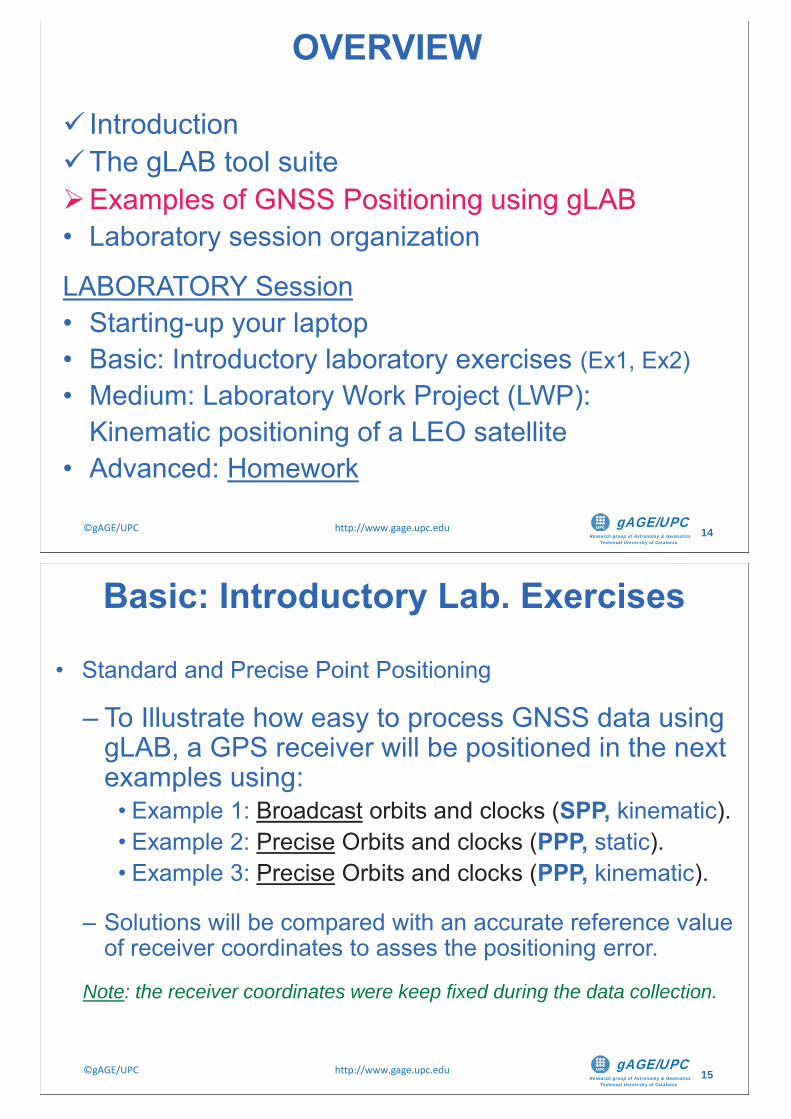
• Standard and Precise Point Positioning
– To Illustrate how easy to process GNSS data using gLAB, a GPS receiver will be positioned in the next examples using:
• Example 1: Broadcast orbits and clocks (SPP, kinematic).• Example 2: Precise Orbits and clocks (PPP, static).• Example 3: Precise Orbits and clocks (PPP, kinematic).
– Solutions will be compared with an accurate reference value of receiver coordinates to asses the positioning error.
Note: the receiver coordinates were keep fixed during the data collection.
Basic: Introductory Lab. Exercises
Research group of Astronomy & GeomaticsTechnical University of Catalonia
gAGE/UPC ©gAGE/UPC http://www.gage.upc.edu 16
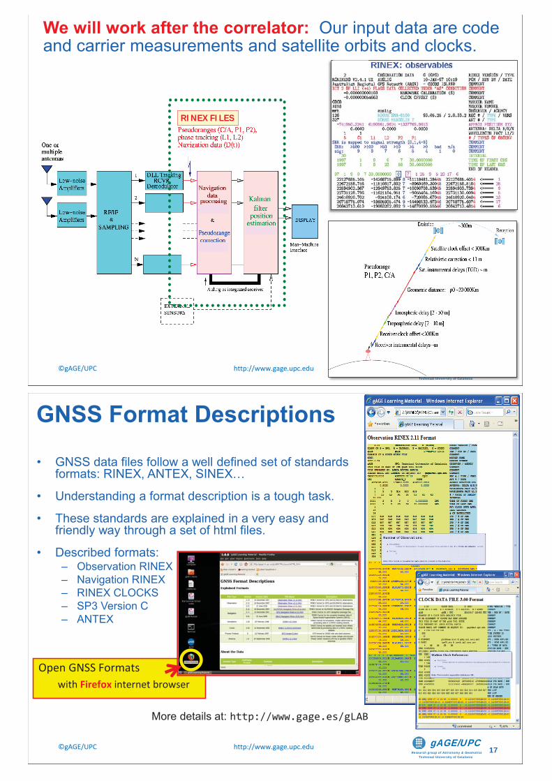
We will work after the correlator: Our input data are code and carrier measurements and satellite orbits and clocks.
16
RINEX FILES
ResearchResearch group fof A tAstronomy && G ticsGeomaticsTechnicTechnicTechnicalalalTechnicTechnicTechnicTechnicTechnicTechnicalalalalalal UniversUniversUnivers yityityityUniversUniversUniversUniversUniversUniversityityityityityity ofofofofofofofofof CatalonCatalonCataloniaiaiaCatalonCatalonCatalonCatalonCatalonCataloniaiaiaiaiaia
gAGE/UPC 1616
Research group of Astronomy & GeomaticsTechnical University of Catalonia
gAGE/UPC ©gAGE/UPC http://www.gage.upc.edu 17
• GNSS data files follow a well defined set of standards formats: RINEX, ANTEX, SINEX…
• Understanding a format description is a tough task.
• These standards are explained in a very easy and friendly way through a set of html files.
• Described formats:– Observation RINEX – Navigation RINEX– RINEX CLOCKS – SP3 Version C– ANTEX
More details at: http://www.gage.es/gLAB
GNSS Format Descriptions
Open GNSS Formatswith Firefox internet browser
Research group of Astronomy & GeomaticsTechnical University of Catalonia
gAGE/UPC ©gAGE/UPC http://www.gage.upc.edu 18
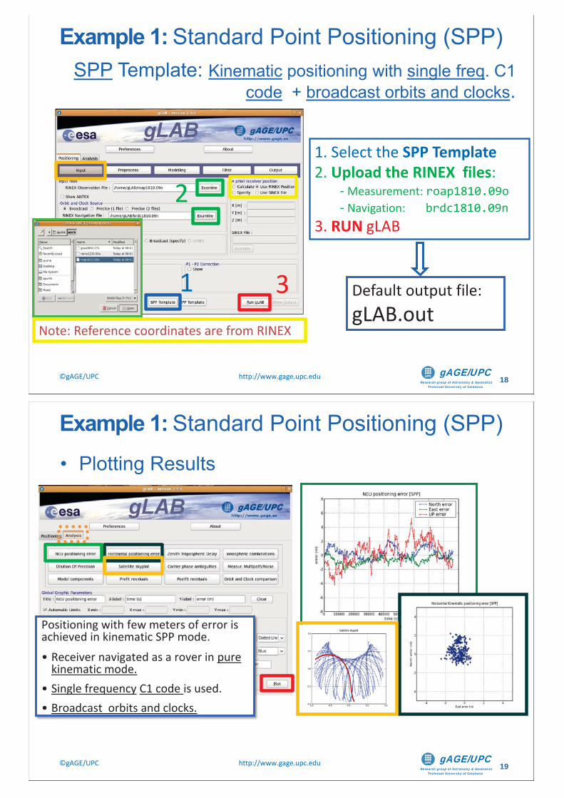
SPP Template: Kinematic positioning with single freq. C1 code + broadcast orbits and clocks.
1. Select the SPP Template 2. Upload the RINEX files:
- Measurement: roap1810.09o- Navigation: brdc1810.09n
3. RUN gLAB
Default output file:gLAB.out
1
2
3Note: Reference coordinates are from RINEX
Example 1: Standard Point Positioning (SPP)
Research group of Astronomy & GeomaticsTechnical University of Catalonia
gAGE/UPC ©gAGE/UPC http://www.gage.upc.edu 19
• Plotting Results
Positioning with few meters of error is achieved in kinematic SPP mode.• Receiver navigated as a rover in pure
kinematic mode.• Single frequency C1 code is used.• Broadcast orbits and clocks.
Example 1: Standard Point Positioning (SPP)
Research group of Astronomy & GeomaticsTechnical University of Catalonia
gAGE/UPC ©gAGE/UPC http://www.gage.upc.edu 20
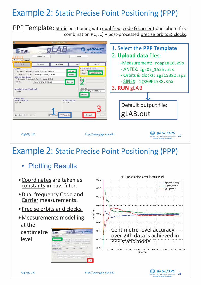
PPP Template: Static positioning with dual freq. code & carrier (ionosphere-free combination PC,LC) + post-processed precise orbits & clocks.
1. Select the PPP Template 2. Upload data files:
-Measurement: roap1810.09o- ANTEX: igs05_1525.atx- Orbits & clocks: igs15382.sp3- SINEX: igs09P1538.snx
3. RUN gLAB
Default output file:gLAB.out 1
2
3
Example 2: Static Precise Point Positioning (PPP)
Research group of Astronomy & GeomaticsTechnical University of Catalonia
gAGE/UPC ©gAGE/UPC http://www.gage.upc.edu 21
• Plotting Results
•Coordinates are taken as constants in nav. filter.
•Dual frequency Code and Carrier measurements.
•Precise orbits and clocks.•Measurements modellingat the centimetrelevel.
Centimetre level accuracy over 24h data is achieved in PPP static mode
Example 2: Static Precise Point Positioning (PPP)
Research group of Astronomy & GeomaticsTechnical University of Catalonia
gAGE/UPC ©gAGE/UPC http://www.gage.upc.edu 22
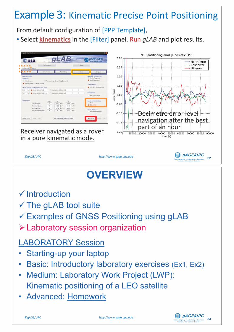
From default configuration of [PPP Template], • Select kinematics in the [Filter] panel. Run gLAB and plot results.
Decimetre error level navigation after the best part of an hourReceiver navigated as a rover
in a pure kinematic mode.
Example 3: Kinematic Precise Point Positioning
Research group of Astronomy & GeomaticsTechnical University of Catalonia
gAGE/UPC ©gAGE/UPC http://www.gage.upc.edu 23
OVERVIEWIntroductionThe gLAB tool suiteExamples of GNSS Positioning using gLABLaboratory session organization
LABORATORY Session• Starting-up your laptop• Basic: Introductory laboratory exercises (Ex1, Ex2)• Medium: Laboratory Work Project (LWP):
Kinematic positioning of a LEO satellite• Advanced: Homework
Research group of Astronomy & GeomaticsTechnical University of Catalonia
gAGE/UPC ©gAGE/UPC http://www.gage.upc.edu 24
• The laboratory session is organized as an assisted activity were a set of exercises must be developed individually or in groups of two.
• As they are conceived as self-learning work, a detailed guide is provided in the slides (pdf file) to develop the exercises.
• A set of questions is presented, and the answers are also included in the slides.
• Teachers will attend individual (or collective) questions that could arise during exercise resolution.
Laboratory session organization
Research group of Astronomy & GeomaticsTechnical University of Catalonia
gAGE/UPC ©gAGE/UPC http://www.gage.upc.edu 25
• The exercises are organized in three different levels of difficulty. The student can choose the level of exercises to do, although at least an introductory exercise is recommended to learn basic gLAB usage.
• 1. Basic: Introductory exercises 1 & 2.They consist of simple exercises to assess the model components for Standard and Precise Point Positioning.“Background information" slides are provided, summarizing the main concepts associated with these exercises.
Brief summaries of fundamentals in backup slides
Laboratory session organization
Research group of Astronomy & GeomaticsTechnical University of Catalonia
gAGE/UPC ©gAGE/UPC http://www.gage.upc.edu 26
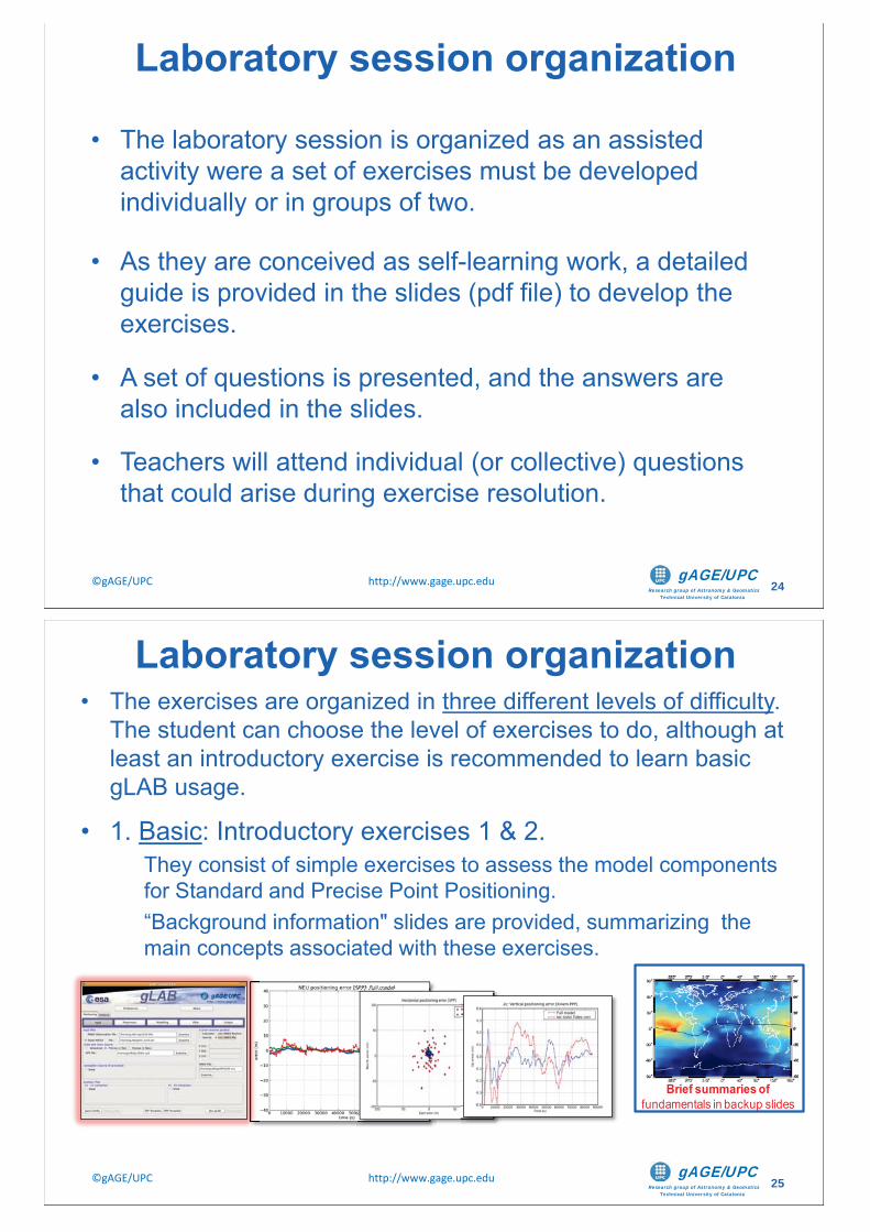
• 2. Medium: Laboratory work project.It consists of the kinematic positioning of a Low Earth Orbit satellite.Different positioning modes are analyzed and different modeling options will be discussed.
Given that session time is limited to 3h, students who feel comfortable using gLAB, can skip part of the previous basic exercises (Ex1, Ex2) and jump to the Lab. Work Project.
Laboratory session organization
Research group of Astronomy & GeomaticsTechnical University of Catalonia
gAGE/UPC ©gAGE/UPC http://www.gage.upc.edu 27
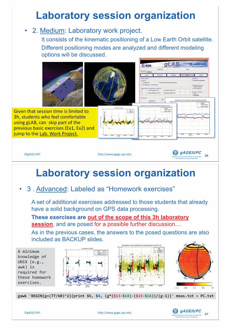
• 3 . Advanced: Labeled as “Homework exercises”
A set of additional exercises addressed to those students that already have a solid background on GPS data processing.These exercises are out of the scope of this 3h laboratory session, and are posed for a possible further discussion…As in the previous cases, the answers to the posed questions are also included as BACKUP slides.
gawk 'BEGIN{g=(77/60)^2}{print $6, $4, (g*($13-$14)-($15-$16))/(g-1)}' meas.txt > PC.txt
A minimum knowledge of UNIX (e.g., awk) is required for these homework exercises.
Laboratory session organization
Research group of Astronomy & GeomaticsTechnical University of Catalonia
gAGE/UPC ©gAGE/UPC http://www.gage.upc.edu 28
IntroductionThe gLAB tool suiteExamples of Positioning with gLABLaboratory session organization
LABORATORY SessionStarting-up your laptop
• Basic: Introductory laboratory exercises (Ex1, Ex2)• Medium: Laboratory Work Project (LWP):
Kinematic positioning of a LEO satellite• Advanced: Homework
OVERVIEW
Research group of Astronomy & GeomaticsTechnical University of Catalonia
gAGE/UPC ©gAGE/UPC http://www.gage.upc.edu 29
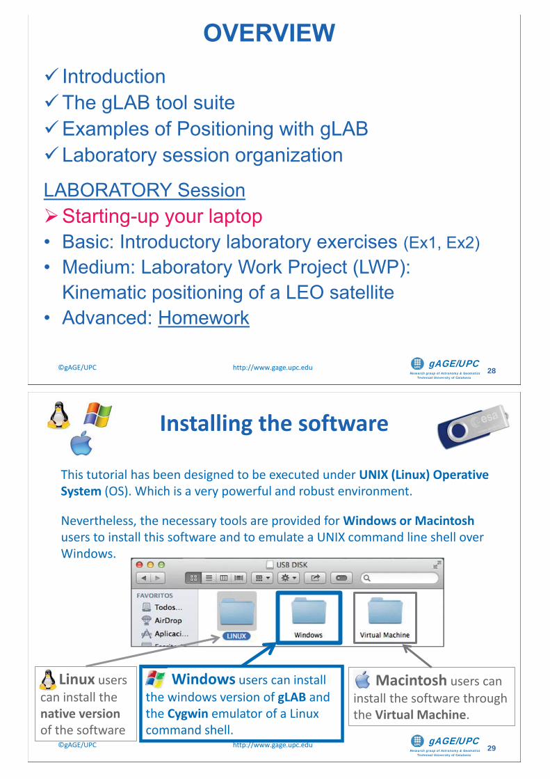
This tutorial has been designed to be executed under UNIX (Linux) Operative System (OS). Which is a very powerful and robust environment.
Nevertheless, the necessary tools are provided for Windows or Macintosh users to install this software and to emulate a UNIX command line shell over Windows.
Installing the software
Macintosh users can install the software through the Virtual Machine.
Windows users can install the windows version of gLAB and the Cygwin emulator of a Linux command shell.
Linux users can install the native version of the software
Research group of Astronomy & GeomaticsTechnical University of Catalonia
gAGE/UPC ©gAGE/UPC http://www.gage.upc.edu 30
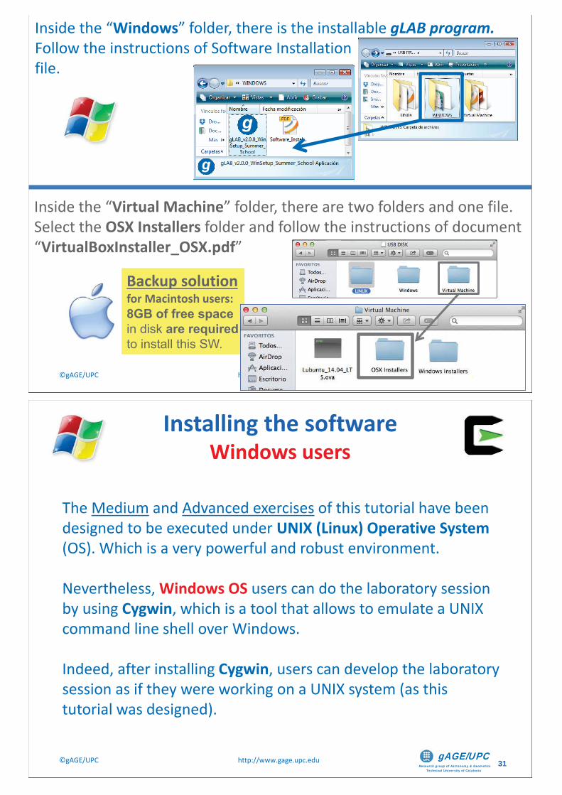
Backup solutionfor Macintosh users:8GB of free space in disk are required to install this SW.
Inside the “Virtual Machine” folder, there are two folders and one file. Select the OSX Installers folder and follow the instructions of document“VirtualBoxInstaller_OSX.pdf”
Inside the “Windows” folder, there is the installable gLAB program. Follow the instructions of Software Installationfile.
Research group of Astronomy & GeomaticsTechnical University of Catalonia
gAGE/UPC ©gAGE/UPC http://www.gage.upc.edu 31
The Medium and Advanced exercises of this tutorial have been designed to be executed under UNIX (Linux) Operative System(OS). Which is a very powerful and robust environment.
Nevertheless, Windows OS users can do the laboratory session by using Cygwin, which is a tool that allows to emulate a UNIX command line shell over Windows.
Indeed, after installing Cygwin, users can develop the laboratory session as if they were working on a UNIX system (as this tutorial was designed).
Installing the softwareWindows users
Research group of Astronomy & GeomaticsTechnical University of Catalonia
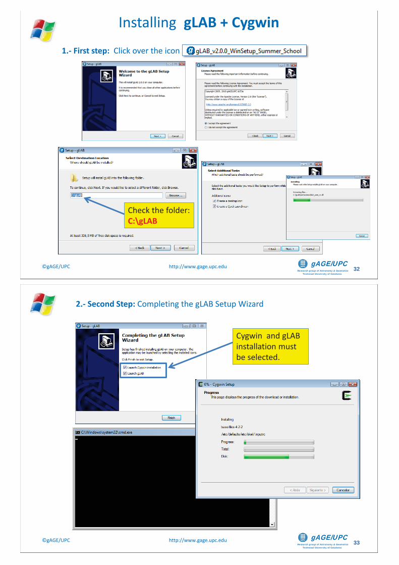
gAGE/UPC ©gAGE/UPC http://www.gage.upc.edu 32
Installing gLAB + Cygwin1.- First step: Click over the icon
Check the folder:C:\gLAB
Research group of Astronomy & GeomaticsTechnical University of Catalonia
gAGE/UPC ©gAGE/UPC http://www.gage.upc.edu 33
2.- Second Step: Completing the gLAB Setup Wizard
Cygwin and gLAB installation must be selected.
Research group of Astronomy & GeomaticsTechnical University of Catalonia
gAGE/UPC ©gAGE/UPC http://www.gage.upc.edu 34
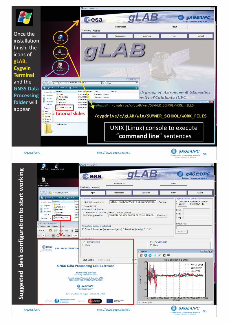
Once the installation finish, the icons of gLAB,CygwinTerminal and the GNSS Data Processing folder will appear.
Tutorial slides /cygdrive/c/gLAB/win/SUMMER_SCHOOL/WORK_FILES
UNIX (Linux) console to execute “command line” sentences
Research group of Astronomy & GeomaticsTechnical University of Catalonia
gAGE/UPC ©gAGE/UPC http://www.gage.upc.edu 35
Sugg
este
d d
esk
conf
igur
atio
n to
star
t wor
king
ESA/ JRC INTERNATIONAL SUMMER SCHOOL ON GNSS 2015 Research group of Astronomy & GeomaticsTechnical University of Catalonia
gAGE/UPC Su
Barcelona, Spain, 31 August - 10 September 2015
Local Organiser: Supported by:
Research group of Astronomy & GeomaticsTechnical University of Catalonia
gAGE/UPC ©gAGE/UPC http://www.gage.upc.edu 36
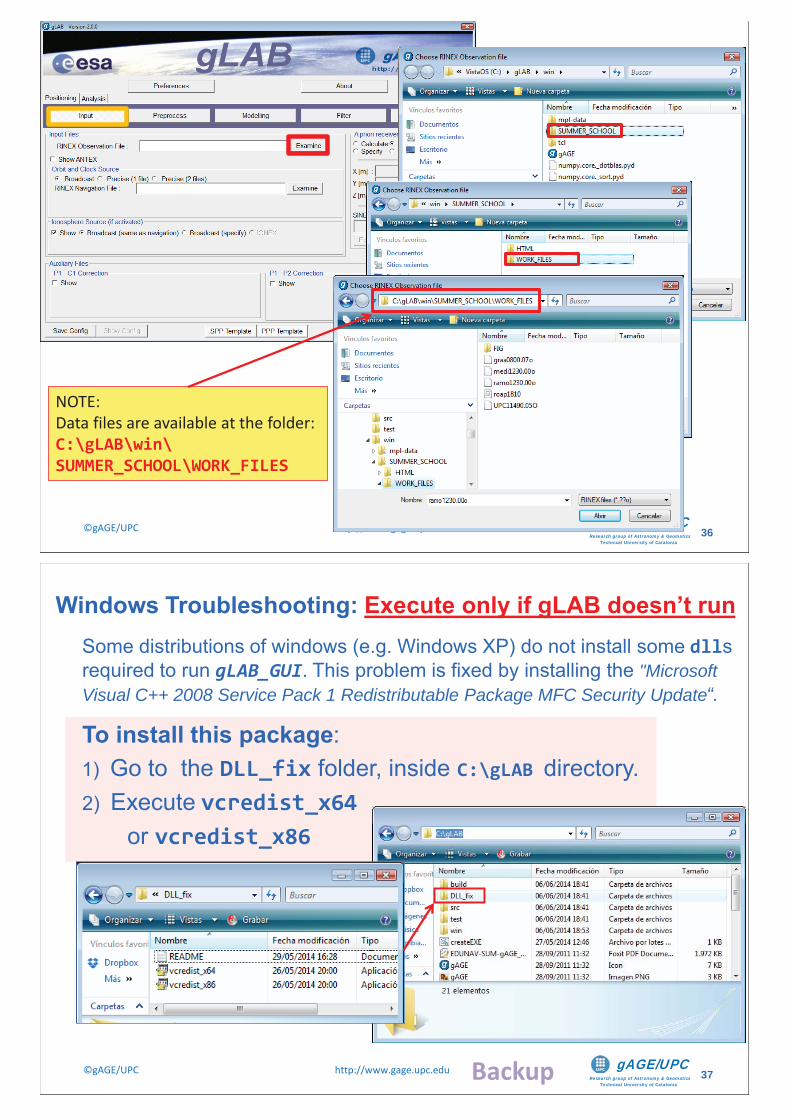
NOTE:Data files are available at the folder:C:\gLAB\win\SUMMER_SCHOOL\WORK_FILES
Research group of Astronomy & GeomaticsTechnical University of Catalonia
gAGE/UPC ©gAGE/UPC http://www.gage.upc.edu 37
Windows Troubleshooting: Execute only if gLAB doesn’t runSome distributions of windows (e.g. Windows XP) do not install some dlls required to run gLAB_GUI. This problem is fixed by installing the "Microsoft Visual C++ 2008 Service Pack 1 Redistributable Package MFC Security Update“.
To install this package:1) Go to the DLL_fix folder, inside C:\gLAB directory. 2) Execute vcredist_x64
or vcredist_x86
Backup
Research group of Astronomy & GeomaticsTechnical University of Catalonia
gAGE/UPC ©gAGE/UPC http://www.gage.upc.edu 38
IntroductionThe gLAB tool suiteExamples of GNSS Positioning using gLABLaboratory session organization
LABORATORY SessionStarting-up your laptopBasic: Introductory laboratory exercises (Ex1, Ex2)
• Medium: Laboratory Work Project (LWP): Kinematic positioning of a LEO satellite
• Advanced: Homework
OVERVIEW
Research group of Astronomy & GeomaticsTechnical University of Catalonia
gAGE/UPC ©gAGE/UPC http://www.gage.upc.edu 39
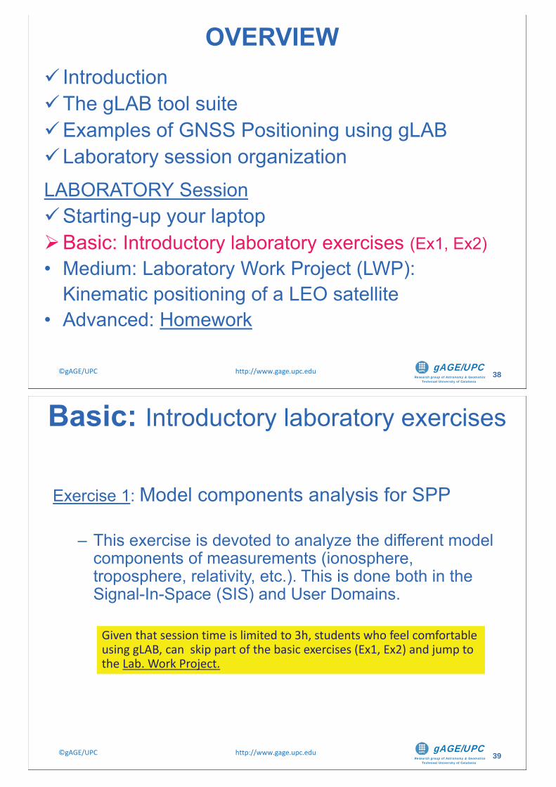
Exercise 1: Model components analysis for SPP
– This exercise is devoted to analyze the different model components of measurements (ionosphere, troposphere, relativity, etc.). This is done both in the Signal-In-Space (SIS) and User Domains.
Basic: Introductory laboratory exercises
Given that session time is limited to 3h, students who feel comfortable using gLAB, can skip part of the basic exercises (Ex1, Ex2) and jump to the Lab. Work Project.
Research group of Astronomy & GeomaticsTechnical University of Catalonia
gAGE/UPC ©gAGE/UPC http://www.gage.upc.edu 40
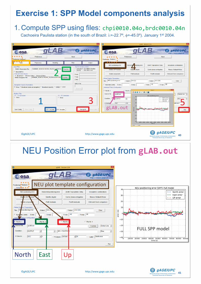
1. Compute SPP using files: chpi0010.04o,brdc0010.04nCachoeira Paulista station (in the south of Brazil: =-22.7º, =-45.0º). January 1st 2004.
Exercise 1: SPP Model components analysis
1
2
3
4
5gLAB.out
Research group of Astronomy & GeomaticsTechnical University of Catalonia
gAGE/UPC ©gAGE/UPC http://www.gage.upc.edu 41
NEU Position Error plot from gLAB.out
North East Up
FULL SPP model
NEU plot template configuration
Research group of Astronomy & GeomaticsTechnical University of Catalonia
gAGE/UPC ©gAGE/UPC http://www.gage.upc.edu 42
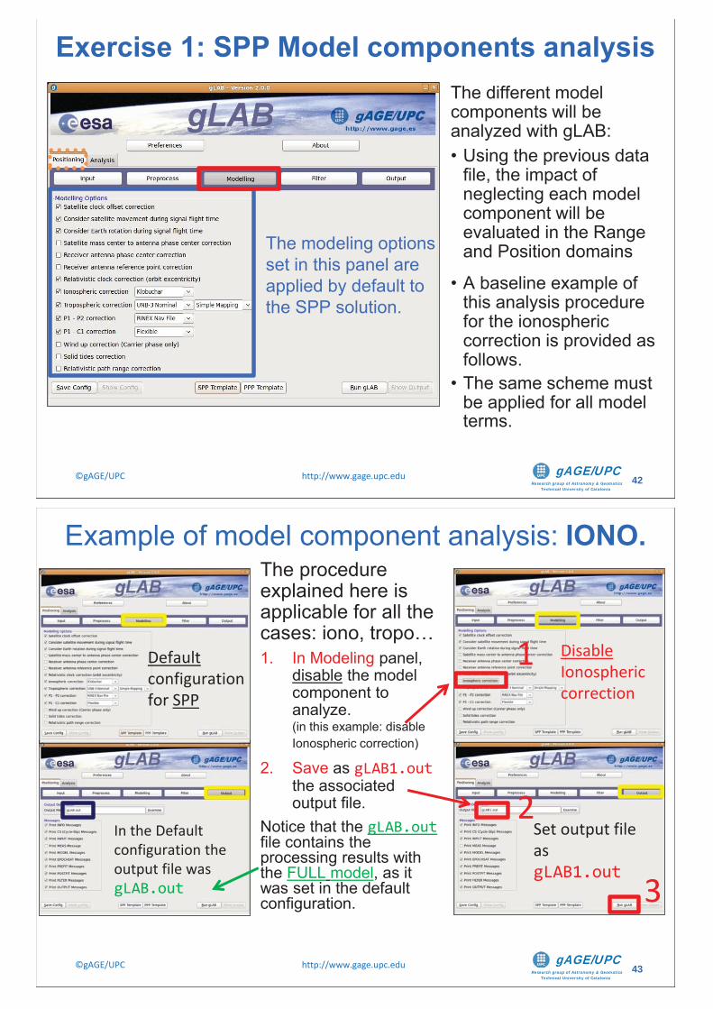
The different model components will be analyzed with gLAB:• Using the previous data
file, the impact of neglecting each model component will be evaluated in the Range and Position domains
• A baseline example of this analysis procedure for the ionosphericcorrection is provided as follows.
• The same scheme must be applied for all model terms.
The modeling options set in this panel are applied by default to the SPP solution.
Exercise 1: SPP Model components analysis
Research group of Astronomy & GeomaticsTechnical University of Catalonia
gAGE/UPC ©gAGE/UPC http://www.gage.upc.edu 43
Example of model component analysis: IONO.
Default configuration for SPP
In the Default configuration the output file was gLAB.out
Set output file as gLAB1.out
Disable Ionosphericcorrection
The procedure explained here is applicable for all the cases: iono, tropo…1. In Modeling panel,
disable the model component to analyze. (in this example: disable Ionospheric correction)
2. Save as gLAB1.outthe associated output file.
Notice that the gLAB.outfile contains the processing results with the FULL model, as it was set in the default configuration.
1
2
3
Research group of Astronomy & GeomaticsTechnical University of Catalonia
gAGE/UPC ©gAGE/UPC http://www.gage.upc.edu 44
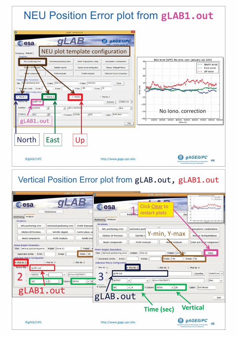
NEU Position Error plot from gLAB1.out
gLAB1.out
North East Up
NEU plot template configuration
No Iono. correction
Research group of Astronomy & GeomaticsTechnical University of Catalonia
gAGE/UPC ©gAGE/UPC http://www.gage.upc.edu 45
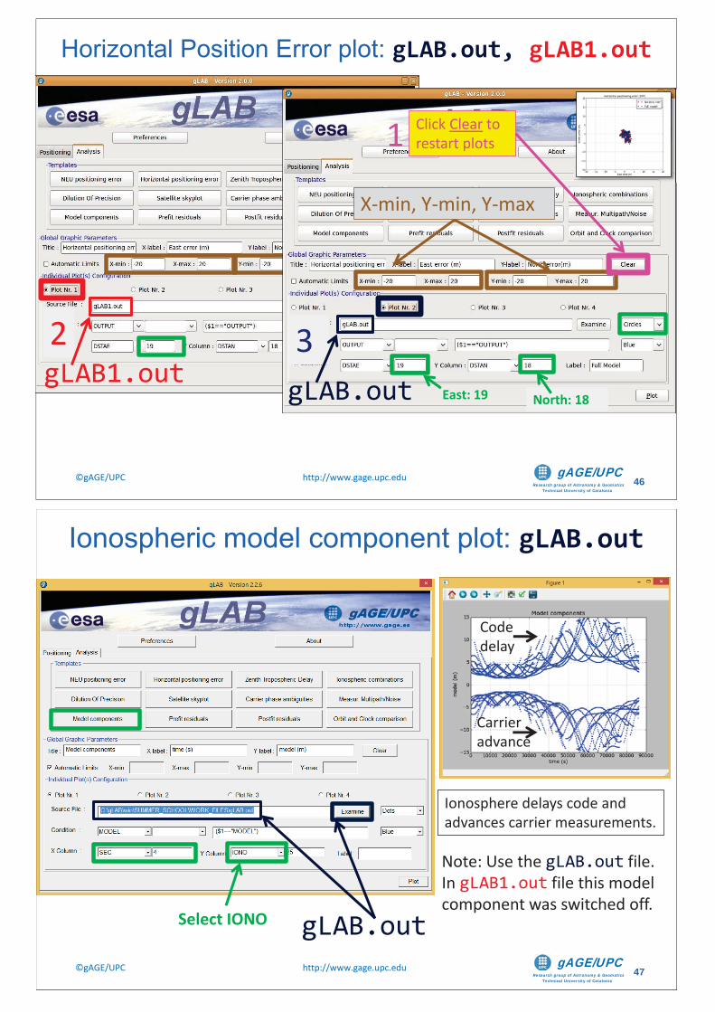
gLAB1.out gLAB.outTime (sec) Vertical
Y-min, Y-max
Vertical Position Error plot from gLAB.out, gLAB1.out
Click Clear to restart plots1
2 3
Research group of Astronomy & GeomaticsTechnical University of Catalonia
gAGE/UPC ©gAGE/UPC http://www.gage.upc.edu 46
Horizontal Position Error plot: gLAB.out, gLAB1.out
gLAB.out East: 19 North: 18
X-min, Y-min, Y-max
Click Clear to restart plots1
2 3gLAB1.out
Research group of Astronomy & GeomaticsTechnical University of Catalonia
gAGE/UPC ©gAGE/UPC http://www.gage.upc.edu 47
Ionospheric model component plot: gLAB.out
gLAB.outSelect IONO
Note: Use the gLAB.out file.In gLAB1.out file this model component was switched off.
Code delay
Ionosphere delays code and advances carrier measurements.
Carrier advance
Research group of Astronomy & GeomaticsTechnical University of Catalonia
gAGE/UPC ©gAGE/UPC http://www.gage.upc.edu 48
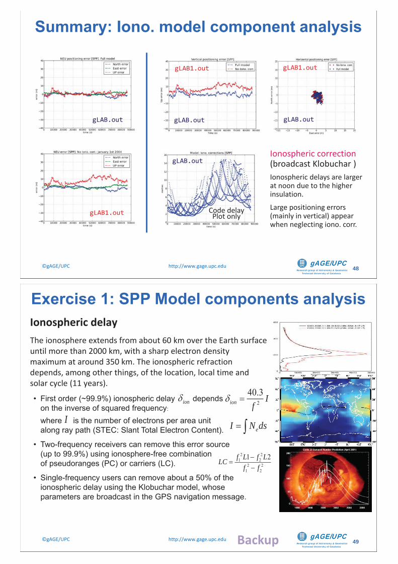
Summary: Iono. model component analysis
gLAB.out
gLAB1.out
gLAB.out
gLAB1.out
gLAB.out
Ionospheric correction (broadcast Klobuchar )Ionospheric delays are larger at noon due to the higher insulation.
Large positioning errors (mainly in vertical) appear when neglecting iono. corr.
Code delay Plot only
gLAB.out
gLAB1.out
Research group of Astronomy & GeomaticsTechnical University of Catalonia
gAGE/UPC ©gAGE/UPC http://www.gage.upc.edu 49
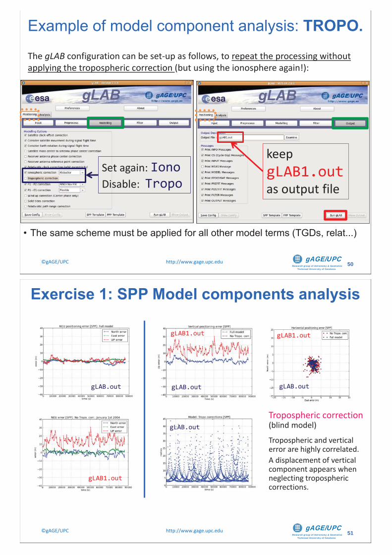
• First order (~99.9%) ionospheric delay depends on the inverse of squared frequency:
where is the number of electrons per area unit along ray path (STEC: Slant Total Electron Content).
• Two-frequency receivers can remove this error source (up to 99.9%) using ionosphere-free combination of pseudoranges (PC) or carriers (LC).
• Single-frequency users can remove about a 50% of the ionospheric delay using the Klobuchar model, whose parameters are broadcast in the GPS navigation message.
240.3
ion If
eI N ds
2 21 2
2 21 2
1 2f L f LLCf f
I
ion
Ionospheric delayThe ionosphere extends from about 60 km over the Earth surface until more than 2000 km, with a sharp electron density maximum at around 350 km. The ionospheric refraction depends, among other things, of the location, local time and solar cycle (11 years).
Exercise 1: SPP Model components analysis
Backup
Research group of Astronomy & GeomaticsTechnical University of Catalonia
gAGE/UPC ©gAGE/UPC http://www.gage.upc.edu 50
keepgLAB1.outas output file
Set again: IonoDisable: Tropo
Example of model component analysis: TROPO.
The gLAB configuration can be set-up as follows, to repeat the processing without applying the tropospheric correction (but using the ionosphere again!):
• The same scheme must be applied for all other model terms (TGDs, relat...)
Research group of Astronomy & GeomaticsTechnical University of Catalonia
gAGE/UPC ©gAGE/UPC http://www.gage.upc.edu 51
gLAB.out
gLAB1.out
gLAB.out
gLAB1.out
gLAB.out gLAB.out
gLAB1.out
Exercise 1: SPP Model components analysis
Tropospheric correction (blind model)
Tropospheric and vertical error are highly correlated. A displacement of vertical component appears when neglecting tropospheric corrections.
Research group of Astronomy & GeomaticsTechnical University of Catalonia
gAGE/UPC ©gAGE/UPC http://www.gage.upc.edu 52
Tropospheric delayThe troposphere is the atmospheric layer placed between Earth’s surface and an
altitude of about 60 km. The effect of troposphere on GNSS signals appears as an extra delay in the
measurement of the signal travelling from satellite to receiver. The tropospheric delay does not depend on frequency and affects both the
pseudorange (code) and carrier phases in the same way. It can be modeled by:– An hydrostatic component, composed of dry gases (mainly nitrogen and oxygen)
in hydrostatic equilibrium. This component can be treated as an ideal gas. Its effects vary with the temperature and atmospheric pressure in a quite predictable manner, and it is the responsible of about 90% of the delay.
– A wet component caused by the water vapor condensed in the form of clouds. It depends on the weather conditions and varies faster than the hydrostatic component and in a quite random way. For high accuracy positioning, this component must be estimated together with the coordinates and other parameters in the navigation filter.
Exercise 1: SPP Model components analysis
Backup
Research group of Astronomy & GeomaticsTechnical University of Catalonia
gAGE/UPC ©gAGE/UPC http://www.gage.upc.edu 53
gLAB.out
gLAB1.out
gLAB.outgLAB1.out
gLAB.out gLAB.out
gLAB1.out
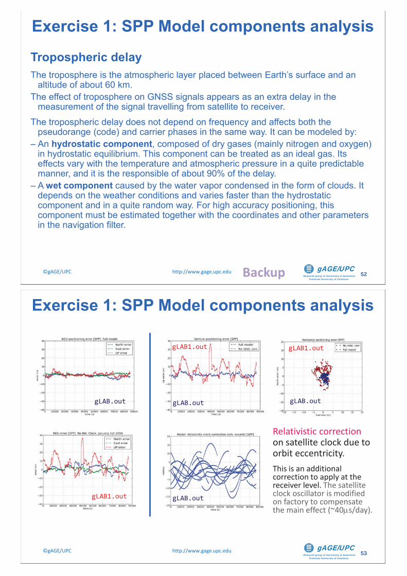
Exercise 1: SPP Model components analysis
Relativistic correction on satellite clock due to orbit eccentricity.This is an additional correction to apply at the receiver level. The satellite clock oscillator is modified on factory to compensate the main effect (~40 s/day).
Research group of Astronomy & GeomaticsTechnical University of Catalonia
gAGE/UPC ©gAGE/UPC http://www.gage.upc.edu 54
Exercise 1: SPP Model components analysis
Relativistic clock correction1) A constant component, depending only on nominal value of satellite’s orbit major semi-axis. It
is corrected modifying satellite’s clock oscillator frequency:
being f0 = 10.23 MHz, we have f=4.464 10-10 f0= 4.57 10-3 Hz. So, satellite should use f’0=10.22999999543 MHz.
2) A periodic component due to orbit eccentricity must be corrected by user receiver:
Being =G ME =3.986005 1014 (m3/s2) the gravitational constant, c =299792458 (m/s) light speed in vacuum, a is orbit’s major semi-axis, e is its eccentricity, E is satellite’s eccentric anomaly, and r and v are satellite’s geocentric position and speed in an inertial system.
2'100 0
20
1 4.464 102
f f v Uf c c
2 sin( ) 2 ( )arel e E metersc c
r v
Backup
Research group of Astronomy & GeomaticsTechnical University of Catalonia
gAGE/UPC ©gAGE/UPC http://www.gage.upc.edu 55
gLAB.out
gLAB1.out
gLAB.outgLAB1.out
gLAB.out gLAB.out
gLAB1.out
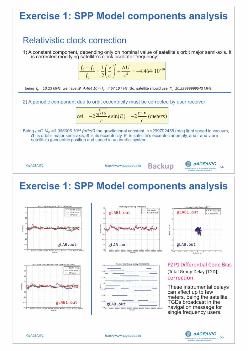
Exercise 1: SPP Model components analysis
P2-P1 Differential Code Bias (Total Group Delay [TGD]) correction.These instrumental delays can affect up to few meters, being the satellite TGDs broadcast in the navigation message for single frequency users.
Research group of Astronomy & GeomaticsTechnical University of Catalonia
gAGE/UPC ©gAGE/UPC http://www.gage.upc.edu 56
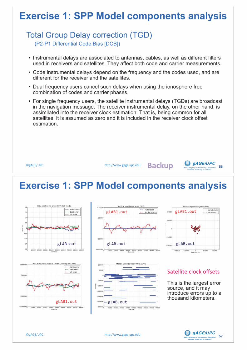
Total Group Delay correction (TGD) (P2-P1 Differential Code Bias [DCB])
• Instrumental delays are associated to antennas, cables, as well as different filters used in receivers and satellites. They affect both code and carrier measurements.
• Code instrumental delays depend on the frequency and the codes used, and are different for the receiver and the satellites.
• Dual frequency users cancel such delays when using the ionosphere free combination of codes and carrier phases.
• For single frequency users, the satellite instrumental delays (TGDs) are broadcast in the navigation message. The receiver instrumental delay, on the other hand, is assimilated into the receiver clock estimation. That is, being common for all satellites, it is assumed as zero and it is included in the receiver clock offset estimation.
Exercise 1: SPP Model components analysis
Backup
Research group of Astronomy & GeomaticsTechnical University of Catalonia
gAGE/UPC ©gAGE/UPC http://www.gage.upc.edu 57
gLAB.out
gLAB1.out
gLAB.outgLAB1.out
gLAB.out gLAB.out
gLAB1.out
Exercise 1: SPP Model components analysis
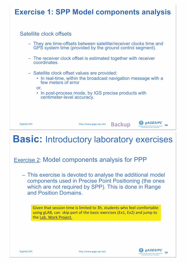
Satellite clock offsets
This is the largest error source, and it may introduce errors up to a thousand kilometers.
Research group of Astronomy & GeomaticsTechnical University of Catalonia
gAGE/UPC ©gAGE/UPC http://www.gage.upc.edu 58
Satellite clock offsets
– They are time-offsets between satellite/receiver clocks time and GPS system time (provided by the ground control segment).
– The receiver clock offset is estimated together with receiver coordinates.
– Satellite clock offset values are provided:• In real-time, within the broadcast navigation message with a
few meters of erroror, • In post-process mode, by IGS precise products with
centimeter-level accuracy.
Exercise 1: SPP Model components analysis
Backup
Research group of Astronomy & GeomaticsTechnical University of Catalonia
gAGE/UPC ©gAGE/UPC http://www.gage.upc.edu 59
Exercise 2: Model components analysis for PPP
– This exercise is devoted to analyse the additional model components used in Precise Point Positioning (the ones which are not required by SPP). This is done in Range and Position Domains.
Basic: Introductory laboratory exercises
Given that session time is limited to 3h, students who feel comfortable using gLAB, can skip part of the basic exercises (Ex1, Ex2) and jump to the Lab. Work Project.
Research group of Astronomy & GeomaticsTechnical University of Catalonia
gAGE/UPC ©gAGE/UPC http://www.gage.upc.edu 60
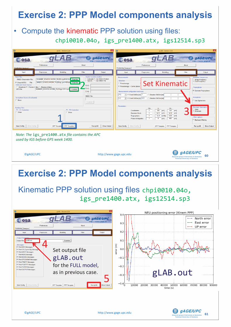
• Compute the kinematic PPP solution using files: chpi0010.04o, igs_pre1400.atx, igs12514.sp3
Note: The igs_pre1400.atx file contains the APC used by IGS before GPS week 1400.
1
2 Set Kinematic
Exercise 2: PPP Model components analysis
3
Research group of Astronomy & GeomaticsTechnical University of Catalonia
gAGE/UPC ©gAGE/UPC http://www.gage.upc.edu 61
Kinematic PPP solution using files chpi0010.04o, igs_pre1400.atx, igs12514.sp3
gLAB.out
Set output file gLAB.outfor the FULL model, as in previous case.
4
5
Exercise 2: PPP Model components analysis
Research group of Astronomy & GeomaticsTechnical University of Catalonia
gAGE/UPC ©gAGE/UPC http://www.gage.upc.edu 62
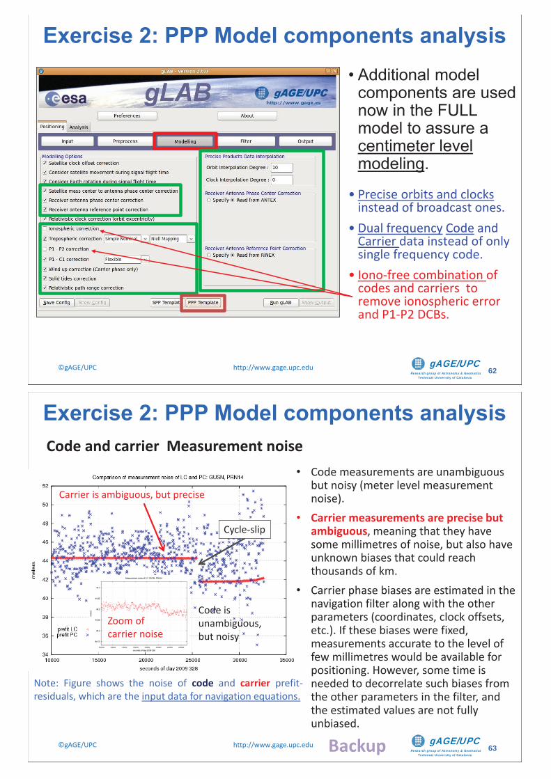
• Additional model components are used now in the FULL model to assure a centimeter level modeling.
• Precise orbits and clocks instead of broadcast ones.
• Dual frequency Code and Carrier data instead of only single frequency code.
• Iono-free combination of codes and carriers to remove ionospheric error and P1-P2 DCBs.
Exercise 2: PPP Model components analysis
Research group of Astronomy & GeomaticsTechnical University of Catalonia
gAGE/UPC ©gAGE/UPC http://www.gage.upc.edu 63
• Code measurements are unambiguous but noisy (meter level measurement noise).
• Carrier measurements are precise but ambiguous, meaning that they have some millimetres of noise, but also have unknown biases that could reach thousands of km.
• Carrier phase biases are estimated in the navigation filter along with the other parameters (coordinates, clock offsets, etc.). If these biases were fixed, measurements accurate to the level of few millimetres would be available for positioning. However, some time is needed to decorrelate such biases from the other parameters in the filter, and the estimated values are not fully unbiased.
Code and carrier Measurement noise
Note: Figure shows the noise of code and carrier prefit-residuals, which are the input data for navigation equations.
Cycle-slip
Code is unambiguous, but noisy
Carrier is ambiguous, but precise
Zoom ofcarrier noise
Exercise 2: PPP Model components analysis
Backup
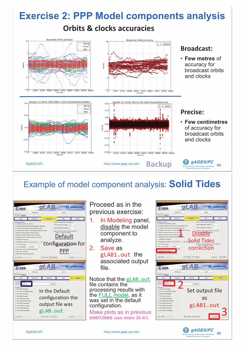
Research group of Astronomy & GeomaticsTechnical University of Catalonia
gAGE/UPC ©gAGE/UPC http://www.gage.upc.edu 64
Exercise 2: PPP Model components analysis
Broadcast:• Few metres of
accuracy for broadcast orbits and clocks
Orbits & clocks accuracies
Precise:• Few centimetres
of accuracy for broadcast orbits and clocks
Backup
Research group of Astronomy & GeomaticsTechnical University of Catalonia
gAGE/UPC ©gAGE/UPC http://www.gage.upc.edu 65
Example of model component analysis: Solid Tides
Default configuration for
PPP
In the Default configuration the output file was gLAB.out
Set output file as
gLAB1.out
DisableSolid Tides correction
Proceed as in the previous exercise:1. In Modeling panel,
disable the model component to analyze.
2. Save as gLAB1.out the associated output file.
Notice that the gLAB.outfile contains the processing results with the FULL model, as it was set in the default configuration.Make plots as in previousexercises (see slides 38-40).
1
2
3
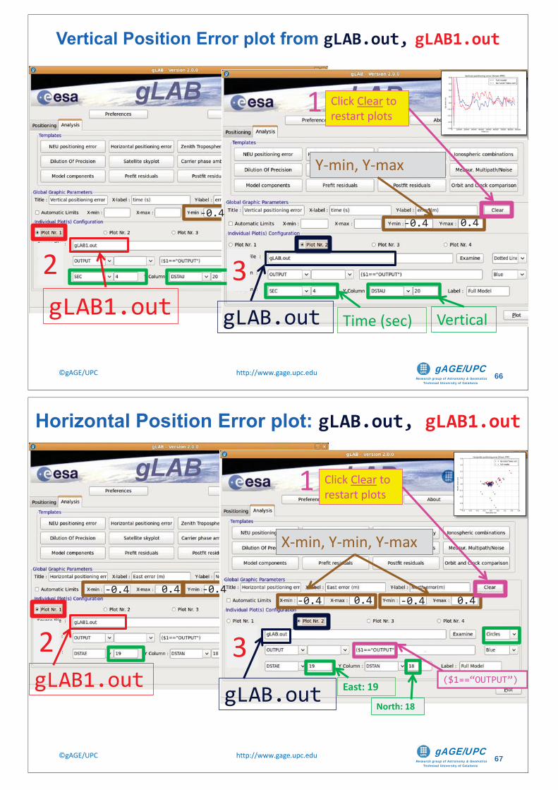
Research group of Astronomy & GeomaticsTechnical University of Catalonia
gAGE/UPC ©gAGE/UPC http://www.gage.upc.edu 66
gLAB1.out gLAB.out Time (sec) Vertical
Y-min, Y-max
Vertical Position Error plot from gLAB.out, gLAB1.out
Click Clear to restart plots
1
2 3
-0.4-0.4 0.4
Research group of Astronomy & GeomaticsTechnical University of Catalonia
gAGE/UPC ©gAGE/UPC http://www.gage.upc.edu 67
Horizontal Position Error plot: gLAB.out, gLAB1.out
gLAB.out East: 19
North: 18
X-min, Y-min, Y-max
($1==“OUTPUT”)
Click Clear to restart plots
1
2 3gLAB1.out
-0.4 0.4 -0.4 0.4-0.4-0.4 0.4
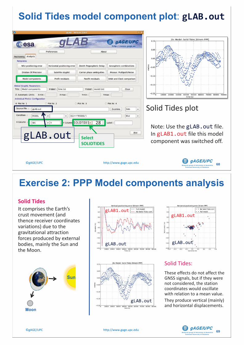
Research group of Astronomy & GeomaticsTechnical University of Catalonia
gAGE/UPC ©gAGE/UPC http://www.gage.upc.edu 68
Solid Tides model component plot: gLAB.out
gLAB.out SelectSOLIDTIDES
Note: Use the gLAB.out file.In gLAB1.out file this model component was switched off.
Solid Tides plot28SOLIDTIDES
Research group of Astronomy & GeomaticsTechnical University of Catalonia
gAGE/UPC ©gAGE/UPC http://www.gage.upc.edu 69
Solid TidesIt comprises the Earth’s crust movement (and thence receiver coordinates variations) due to the gravitational attraction forces produced by external bodies, mainly the Sun and the Moon.
Sun
Moon
gLAB.out
gLAB1.out
gLAB.out
Solid Tides:These effects do not affect the GNSS signals, but if they were not considered, the station coordinates would oscillate with relation to a mean value.They produce vertical (mainly) and horizontal displacements.
Exercise 2: PPP Model components analysis
gLAB.out
gLAB1.out
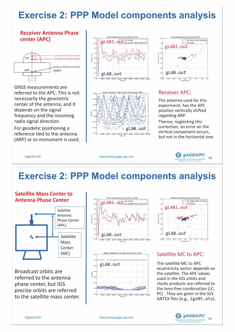
Research group of Astronomy & GeomaticsTechnical University of Catalonia
gAGE/UPC ©gAGE/UPC http://www.gage.upc.edu 70
Receiver Antenna Phase center (APC)
GNSS measurements are referred to the APC. This is not necessarily the geometric center of the antenna, and it depends on the signal frequency and the incoming radio signal direction. For geodetic positioning a reference tied to the antenna (ARP) or to monument is used.
Receiver APC:The antenna used for this experiment, has the APC position vertically shifted regarding ARP.Thence, neglecting this correction, an error on the vertical component occurs, but not in the horizontal one.
(ARP)
APC
ARP
L2 Antenna Phase centerL1 Antenna Phase center
Antenna Reference Point (ARP)
Exercise 2: PPP Model components analysis
gLAB.out
gLAB1.out
gLAB.out
gLAB1.out
gLAB.out
Research group of Astronomy & GeomaticsTechnical University of Catalonia
gAGE/UPC ©gAGE/UPC http://www.gage.upc.edu 71
Satellite Mass Center to Antenna Phase Center
Satellite Mass Center(MC)
Broadcast orbits are referred to the antenna phase center, but IGS precise orbits are referred to the satellite mass center.
gLAB.out
Satellite MC to APC:The satellite MC to APC eccentricity vector depends on the satellite. The APC values used in the IGS orbits and clocks products are referred to the iono-free combination (LC, PC) . They are given in the IGS ANTEX files (e.g., igs05.atx).
Satellite AntennaPhase Center (APC)
Exercise 2: PPP Model components analysis
gLAB.outgLAB.out
gLAB1.out gLAB1.out
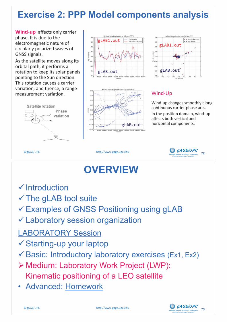
Research group of Astronomy & GeomaticsTechnical University of Catalonia
gAGE/UPC ©gAGE/UPC http://www.gage.upc.edu 72
Wind-up affects only carrier phase. It is due to the electromagnetic nature of circularly polarized waves of GNSS signals.As the satellite moves along its orbital path, it performs a rotation to keep its solar panels pointing to the Sun direction. This rotation causes a carrier variation, and thence, a range measurement variation.
Satellite rotationPhase
variation
gLAB.out
Wind-UpWind-up changes smoothly along continuous carrier phase arcs. In the position domain, wind-up affects both vertical and horizontal components.
Exercise 2: PPP Model components analysis
gLAB.out
gLAB1.out
gLAB.out
gLAB1.out
Research group of Astronomy & GeomaticsTechnical University of Catalonia
gAGE/UPC ©gAGE/UPC http://www.gage.upc.edu 73
IntroductionThe gLAB tool suiteExamples of GNSS Positioning using gLABLaboratory session organization
LABORATORY SessionStarting-up your laptopBasic: Introductory laboratory exercises (Ex1, Ex2)Medium: Laboratory Work Project (LWP): Kinematic positioning of a LEO satellite
• Advanced: Homework
OVERVIEW
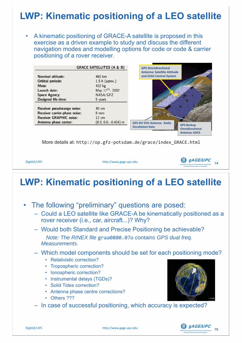
Research group of Astronomy & GeomaticsTechnical University of Catalonia
gAGE/UPC ©gAGE/UPC http://www.gage.upc.edu 74
• A kinematic positioning of GRACE-A satellite is proposed in this exercise as a driven example to study and discuss the different navigation modes and modelling options for code or code & carrier positioning of a rover receiver.
More details at: http://op.gfz-potsdam.de/grace/index_GRACE.html
LWP: Kinematic positioning of a LEO satellite
GPS OmnidirectionalAntenna: Satellite Attitude and Orbit Control System
GPS Backup OmnidirectionalAntenna: AOCS
GPS 45º FOV Antenna: Radio Occultation Data
Research group of Astronomy & GeomaticsTechnical University of Catalonia
gAGE/UPC ©gAGE/UPC http://www.gage.upc.edu 75
• The following “preliminary” questions are posed:– Could a LEO satellite like GRACE-A be kinematically positioned as a
rover receiver (i.e., car, aircraft...)? Why?– Would both Standard and Precise Positioning be achievable?
Note: The RINEX file graa0800.07o contains GPS dual freq. Measurements.
– Which model components should be set for each positioning mode?• Relativistic correction?• Tropospheric correction?• Ionospheric correction?• Instrumental delays (TGDs)?• Solid Tides correction?• Antenna phase centre corrections?• Others ???
– In case of successful positioning, which accuracy is expected?
LWP: Kinematic positioning of a LEO satellite
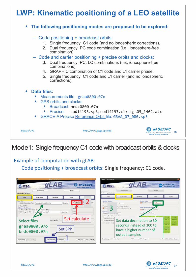
Research group of Astronomy & GeomaticsTechnical University of Catalonia
gAGE/UPC ©gAGE/UPC http://www.gage.upc.edu 76
The following positioning modes are proposed to be explored:
– Code positioning + broadcast orbits:1. Single frequency: C1 code (and no ionospheric corrections).2. Dual frequency: PC code combination (i.e., ionosphere-free
combination).– Code and carrier positioning + precise orbits and clocks:
3. Dual frequency: PC, LC combinations (i.e., ionosphere-free combinations).
4. GRAPHIC combination of C1 code and L1 carrier phase.5. Single frequency: C1 code and L1 carrier (and no ionospheric
corrections).
Data files: Measurements file: graa0800.07oGPS orbits and clocks:
Broadcast: brdc0800.07nPrecise: cod14193.sp3, cod14193.clk, igs05_1402.atx
GRACE-A Precise Reference Orbit file: GRAA_07_080.sp3
LWP: Kinematic positioning of a LEO satellite
Research group of Astronomy & GeomaticsTechnical University of Catalonia
gAGE/UPC ©gAGE/UPC http://www.gage.upc.edu 77
Example of computation with gLAB: Code positioning + broadcast orbits: Single frequency: C1 code.
Set calculateSelect files graa0800.07obrdc0800.07n
Set SPPSet data decimation to 30 seconds instead of 300 to have a higher number of output samples
Mode1: Single frequency C1 code with broadcast orbits & clocks
1
2
Set SPP
3
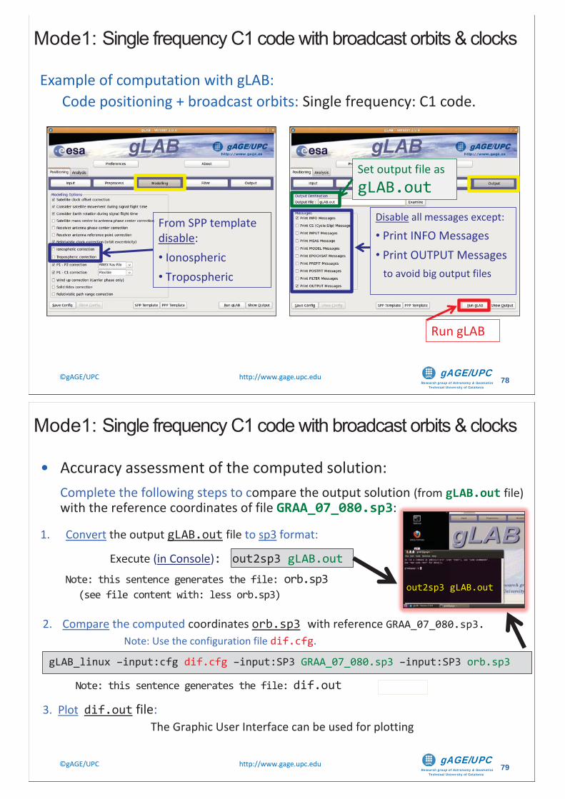
Research group of Astronomy & GeomaticsTechnical University of Catalonia
gAGE/UPC ©gAGE/UPC http://www.gage.upc.edu 78
Example of computation with gLAB: Code positioning + broadcast orbits: Single frequency: C1 code.
Disable all messages except:
• Print INFO Messages• Print OUTPUT Messages
to avoid big output files
Run gLAB
From SPP template disable:• Ionospheric• Tropospheric
Set output file asgLAB.out
Mode1: Single frequency C1 code with broadcast orbits & clocks
Research group of Astronomy & GeomaticsTechnical University of Catalonia
gAGE/UPC ©gAGE/UPC http://www.gage.upc.edu 79
• Accuracy assessment of the computed solution:Complete the following steps to compare the output solution (from gLAB.out file) with the reference coordinates of file GRAA_07_080.sp3:
1. Convert the output gLAB.out file to sp3 format:
Execute (in Console): out2sp3 gLAB.outNote: this sentence generates the file: orb.sp3
(see file content with: less orb.sp3)
:
out2sp3 gLAB.out
2. Compare the computed coordinates orb.sp3 with reference GRAA_07_080.sp3. Note: Use the configuration file dif.cfg.
gLAB_linux –input:cfg dif.cfg –input:SP3 GRAA_07_080.sp3 –input:SP3 orb.sp3
Note: this sentence generates the file: dif.out
3. Plot dif.out file:The Graphic User Interface can be used for plotting
Mode1: Single frequency C1 code with broadcast orbits & clocks
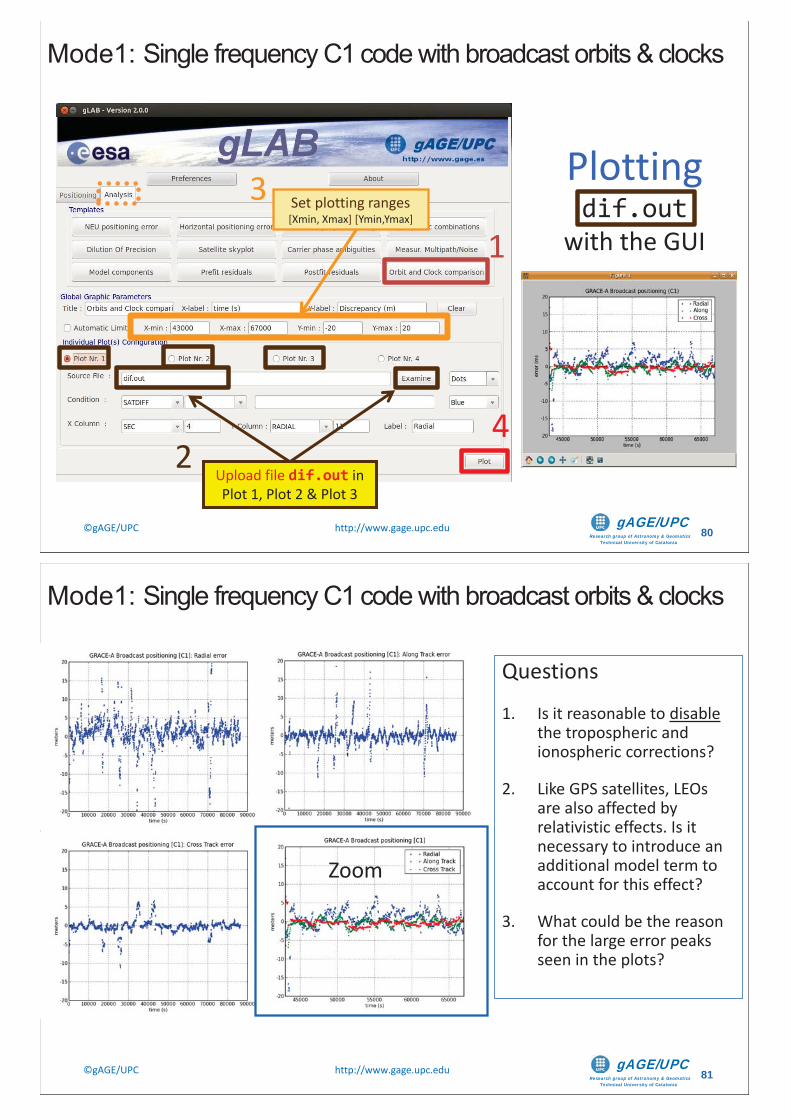
Research group of Astronomy & GeomaticsTechnical University of Catalonia
gAGE/UPC ©gAGE/UPC http://www.gage.upc.edu 80
Set plotting ranges[Xmin, Xmax] [Ymin,Ymax]
Plotting dif.out
with the GUI
Upload file dif.out in Plot 1, Plot 2 & Plot 3
1
2
3
4
Mode1: Single frequency C1 code with broadcast orbits & clocks
Research group of Astronomy & GeomaticsTechnical University of Catalonia
gAGE/UPC ©gAGE/UPC http://www.gage.upc.edu 81
Questions
1. Is it reasonable to disablethe tropospheric and ionospheric corrections?
2. Like GPS satellites, LEOs are also affected by relativistic effects. Is it necessary to introduce an additional model term to account for this effect?
3. What could be the reason for the large error peaks seen in the plots?
Zoom
Mode1: Single frequency C1 code with broadcast orbits & clocks
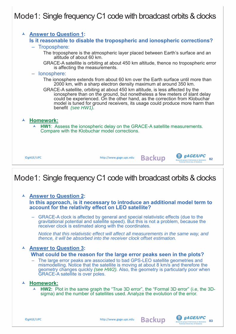
Research group of Astronomy & GeomaticsTechnical University of Catalonia
gAGE/UPC ©gAGE/UPC http://www.gage.upc.edu 82
Answer to Question 1: Is it reasonable to disable the tropospheric and ionospheric corrections?– Troposphere:
The troposphere is the atmospheric layer placed between Earth’s surface and an altitude of about 60 km.
GRACE-A satellite is orbiting at about 450 km altitude, thence no tropospheric error is affecting the measurements.
– Ionosphere:The ionosphere extends from about 60 km over the Earth surface until more than
2000 km, with a sharp electron density maximum at around 350 km. GRACE-A satellite, orbiting at about 450 km altitude, is less affected by the
ionosphere than on the ground, but nonetheless a few meters of slant delay could be experienced. On the other hand, as the correction from Klobucharmodel is tuned for ground receivers, its usage could produce more harm than benefit (see HW1).
Homework:HW1: Assess the ionospheric delay on the GRACE-A satellite measurements. Compare with the Klobuchar model corrections.
Mode1: Single frequency C1 code with broadcast orbits & clocks
Backup
Research group of Astronomy & GeomaticsTechnical University of Catalonia
gAGE/UPC ©gAGE/UPC http://www.gage.upc.edu 83
Answer to Question 2: In this approach, is it necessary to introduce an additional model term to account for the relativity effect on LEO satellite?– GRACE-A clock is affected by general and special relativistic effects (due to the
gravitational potential and satellite speed). But this is not a problem, because the receiver clock is estimated along with the coordinates. Notice that this relativistic effect will affect all measurements in the same way, and thence, it will be absorbed into the receiver clock offset estimation.
Answer to Question 3: What could be the reason for the large error peaks seen in the plots?– The large error peaks are associated to bad GPS-LEO satellite geometries and
mismodelling. Notice that the satellite is moving at about 8 km/s and therefore the geometry changes quickly (see HW2). Also, the geometry is particularly poor when GRACE-A satellite is over poles.
Homework:HW2: Plot in the same graph the “True 3D error”, the “Formal 3D error” (i.e, the 3D-sigma) and the number of satellites used. Analyze the evolution of the error.
Mode1: Single frequency C1 code with broadcast orbits & clocks
Backup
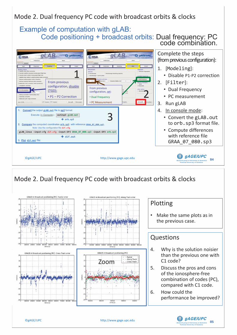
Research group of Astronomy & GeomaticsTechnical University of Catalonia
gAGE/UPC ©gAGE/UPC http://www.gage.upc.edu 84
1. Convert the output gLAB.out file to sp3 format:
Execute (in Console): out2sp3 gLAB.out
orb.sp3
2. Compare the computed coordinates orb.sp3 with reference GRAA_07_080.sp3. Note: Use the configuration file dif.cfg.
gLAB_linux –input:cfg dif.cfg –input:SP3 GRAA_07_080.sp3 –input:SP3 orb.sp3
dif.out3. Plot dif.out file:
Example of computation with gLAB: Code positioning + broadcast orbits: Dual frequency: PC
code combination.
1
3
Complete the steps (from previous configuration):1. [Modeling]:
• Disable P1-P2 correction2. [Filter]:
• Dual Frequency• PC measurement
3. Run gLAB4. In console mode:
• Convert the gLAB.outto orb.sp3 format file.
• Compute differences with reference file GRAA_07_080.sp3
Mode 2. Dual frequency PC code with broadcast orbits & clocks
From previous configuration, disable (TGD):
• P1 – P2 Correction 2From previous configuration, set:
• Dual Frequency
• PC Measurement
Research group of Astronomy & GeomaticsTechnical University of Catalonia
gAGE/UPC ©gAGE/UPC http://www.gage.upc.edu 85
Questions4. Why is the solution noisier
than the previous one with C1 code?
5. Discuss the pros and cons of the ionosphere-free combination of codes (PC), compared with C1 code.
6. How could the performance be improved?
Plotting• Make the same plots as in
the previous case.
Mode 2. Dual frequency PC code with broadcast orbits & clocks
Zoom
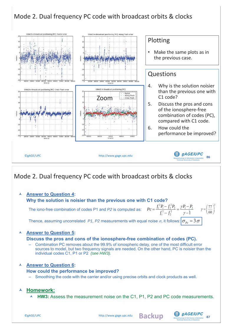
Research group of Astronomy & GeomaticsTechnical University of Catalonia
gAGE/UPC ©gAGE/UPC http://www.gage.upc.edu 86
Questions4. Why is the solution noisier
than the previous one with C1 code?
5. Discuss the pros and cons of the ionosphere-free combination of codes (PC), compared with C1 code.
6. How could the performance be improved?
Plotting• Make the same plots as in
the previous case.
Mode 2. Dual frequency PC code with broadcast orbits & clocks
Zoom
Research group of Astronomy & GeomaticsTechnical University of Catalonia
gAGE/UPC ©gAGE/UPC http://www.gage.upc.edu 87
Answer to Question 4: Why the solution is noisier than the previous one with C1 code?
The iono-free combination of codes P1 and P2 is computed as: ;
Thence, assuming uncorrelated P1, P2 measurements with equal noise , it follows:
Answer to Question 5: Discuss the pros and cons of the ionosphere-free combination of codes (PC).– Combination PC removes about the 99.9% of ionospheric delay, one of the most difficult error
sources to model, but two frequency signals are needed. On the other hand, PC is noisier than the individual codes C1, P1 or P2 (see HW3).
Answer to Question 6: How could the performance be improved?– Smoothing the code with the carrier and/or using precise orbits and clock products as well.
Homework:HW3: Assess the measurement noise on the C1, P1, P2 and PC code measurements.
2 21 1 2 2 1 2
2 21 2 1
f P f P P PPcf f
27760
3Pc
Mode 2. Dual frequency PC code with broadcast orbits & clocks
Backup
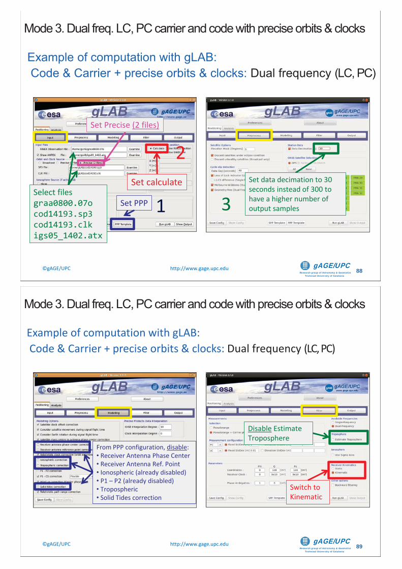
Research group of Astronomy & GeomaticsTechnical University of Catalonia
gAGE/UPC ©gAGE/UPC http://www.gage.upc.edu 88
Example of computation with gLAB: Code & Carrier + precise orbits & clocks: Dual frequency (LC, PC)
Set calculateSelect files graa0800.07ocod14193.sp3cod14193.clkigs05_1402.atx
Set PPP Set SPP
Set data decimation to 30 seconds instead of 300 to have a higher number of output samples
Mode 3. Dual freq. LC, PC carrier and code with precise orbits & clocks
Set Precise (2 files)
1
2
3
Research group of Astronomy & GeomaticsTechnical University of Catalonia
gAGE/UPC ©gAGE/UPC http://www.gage.upc.edu 89
From PPP configuration, disable:• Receiver Antenna Phase Center• Receiver Antenna Ref. Point• Ionospheric (already disabled)• P1 – P2 (already disabled)• Tropospheric• Solid Tides correction
Switch to Kinematic
Disable Estimate Troposphere
Mode 3. Dual freq. LC, PC carrier and code with precise orbits & clocks
Example of computation with gLAB: Code & Carrier + precise orbits & clocks: Dual frequency (LC, PC)
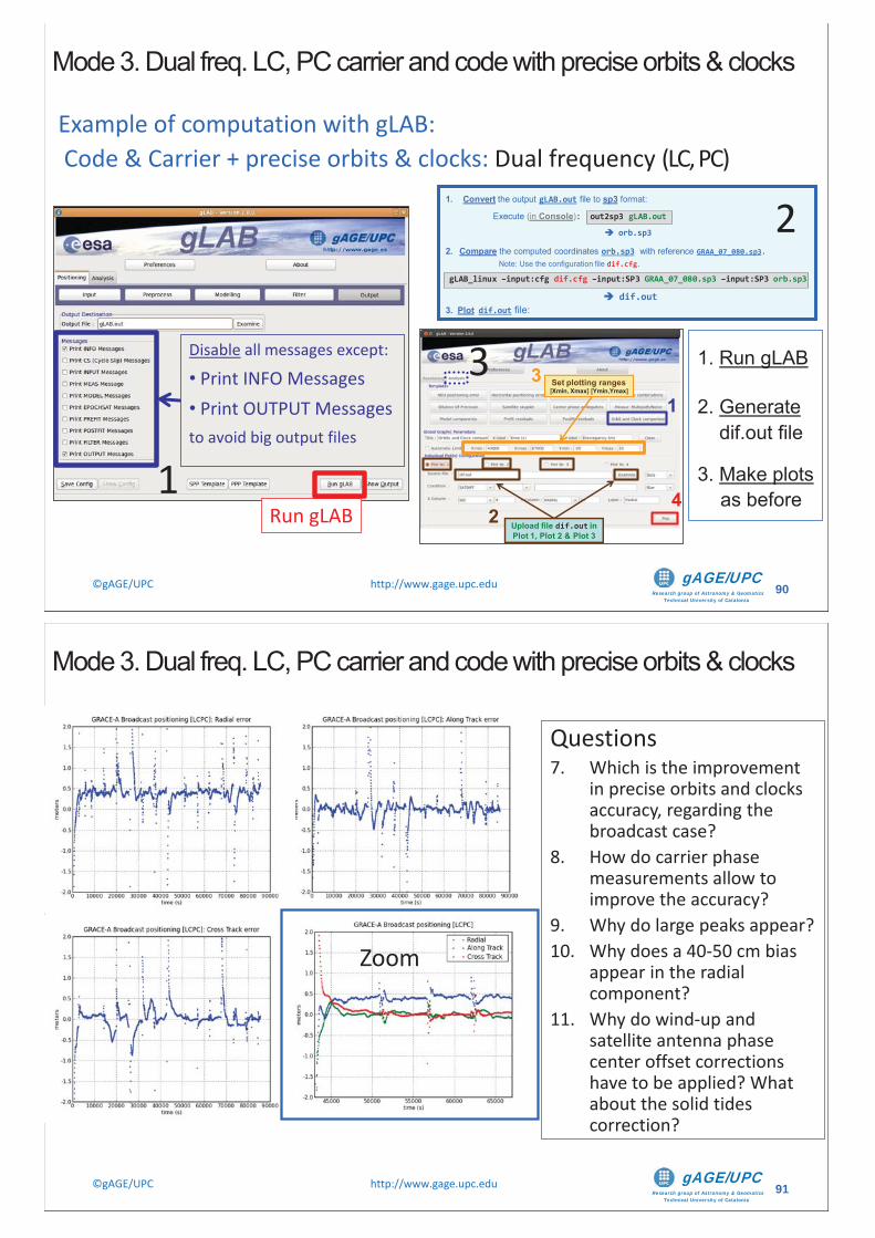
Research group of Astronomy & GeomaticsTechnical University of Catalonia
gAGE/UPC ©gAGE/UPC http://www.gage.upc.edu 90
1. Run gLAB
2. Generatedif.out file
3. Make plotsas before
Set plotting ranges[Xmin, Xmax] [Ymin,Ymax]
Upload file dif.out in Plot 1, Plot 2 & Plot 3
1
2
3
4
1. Convert the output gLAB.out file to sp3 format:
Execute (in Console): out2sp3 gLAB.out
orb.sp3
2. Compare the computed coordinates orb.sp3 with reference GRAA_07_080.sp3. Note: Use the configuration file dif.cfg.
gLAB_linux –input:cfg dif.cfg –input:SP3 GRAA_07_080.sp3 –input:SP3 orb.sp3
dif.out3. Plot dif.out file:
Disable all messages except:
• Print INFO Messages• Print OUTPUT Messagesto avoid big output files
Run gLAB
2
3
1
Mode 3. Dual freq. LC, PC carrier and code with precise orbits & clocks
Example of computation with gLAB: Code & Carrier + precise orbits & clocks: Dual frequency (LC, PC)
Research group of Astronomy & GeomaticsTechnical University of Catalonia
gAGE/UPC ©gAGE/UPC http://www.gage.upc.edu 91
Questions7. Which is the improvement
in precise orbits and clocks accuracy, regarding the broadcast case?
8. How do carrier phase measurements allow to improve the accuracy?
9. Why do large peaks appear?10. Why does a 40-50 cm bias
appear in the radial component?
11. Why do wind-up and satellite antenna phase center offset corrections have to be applied? What about the solid tides correction?
Mode 3. Dual freq. LC, PC carrier and code with precise orbits & clocks
Zoom
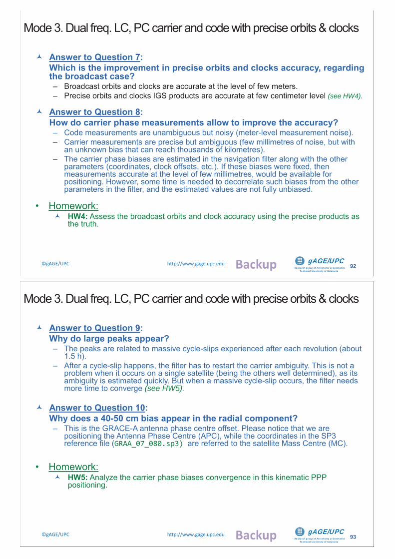
Research group of Astronomy & GeomaticsTechnical University of Catalonia
gAGE/UPC ©gAGE/UPC http://www.gage.upc.edu 92
Answer to Question 7: Which is the improvement in precise orbits and clocks accuracy, regarding the broadcast case?– Broadcast orbits and clocks are accurate at the level of few meters.– Precise orbits and clocks IGS products are accurate at few centimeter level (see HW4).
Answer to Question 8: How do carrier phase measurements allow to improve the accuracy?– Code measurements are unambiguous but noisy (meter-level measurement noise).– Carrier measurements are precise but ambiguous (few millimetres of noise, but with
an unknown bias that can reach thousands of kilometres).– The carrier phase biases are estimated in the navigation filter along with the other
parameters (coordinates, clock offsets, etc.). If these biases were fixed, then measurements accurate at the level of few millimetres, would be available for positioning. However, some time is needed to decorrelate such biases from the other parameters in the filter, and the estimated values are not fully unbiased.
• Homework:HW4: Assess the broadcast orbits and clock accuracy using the precise products as the truth.
Mode 3. Dual freq. LC, PC carrier and code with precise orbits & clocks
Backup
Research group of Astronomy & GeomaticsTechnical University of Catalonia
gAGE/UPC ©gAGE/UPC http://www.gage.upc.edu 93
Answer to Question 9: Why do large peaks appear?– The peaks are related to massive cycle-slips experienced after each revolution (about
1.5 h). – After a cycle-slip happens, the filter has to restart the carrier ambiguity. This is not a
problem when it occurs on a single satellite (being the others well determined), as its ambiguity is estimated quickly. But when a massive cycle-slip occurs, the filter needs more time to converge (see HW5).
Answer to Question 10: Why does a 40-50 cm bias appear in the radial component?– This is the GRACE-A antenna phase centre offset. Please notice that we are
positioning the Antenna Phase Centre (APC), while the coordinates in the SP3 reference file (GRAA_07_080.sp3) are referred to the satellite Mass Centre (MC).
• Homework:HW5: Analyze the carrier phase biases convergence in this kinematic PPP positioning.
Mode 3. Dual freq. LC, PC carrier and code with precise orbits & clocks
Backup
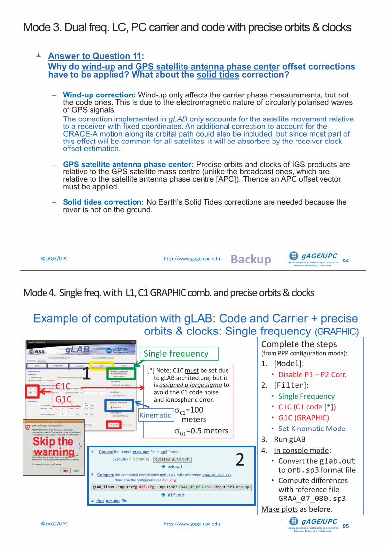
Research group of Astronomy & GeomaticsTechnical University of Catalonia
gAGE/UPC ©gAGE/UPC http://www.gage.upc.edu 94
Answer to Question 11: Why do wind-up and GPS satellite antenna phase center offset corrections have to be applied? What about the solid tides correction?
– Wind-up correction: Wind-up only affects the carrier phase measurements, but not the code ones. This is due to the electromagnetic nature of circularly polarised waves of GPS signals.The correction implemented in gLAB only accounts for the satellite movement relative to a receiver with fixed coordinates. An additional correction to account for the GRACE-A motion along its orbital path could also be included, but since most part of this effect will be common for all satellites, it will be absorbed by the receiver clock offset estimation.
– GPS satellite antenna phase center: Precise orbits and clocks of IGS products are relative to the GPS satellite mass centre (unlike the broadcast ones, which are relative to the satellite antenna phase centre [APC]). Thence an APC offset vector must be applied.
– Solid tides correction: No Earth’s Solid Tides corrections are needed because the rover is not on the ground.
Mode 3. Dual freq. LC, PC carrier and code with precise orbits & clocks
Backup
Research group of Astronomy & GeomaticsTechnical University of Catalonia
gAGE/UPC ©gAGE/UPC http://www.gage.upc.edu 95
Example of computation with gLAB: Code and Carrier + precise orbits & clocks: Single frequency (GRAPHIC)
1. Convert the output gLAB.out file to sp3 format:
Execute (in Console): out2sp3 gLAB.out
orb.sp3
2. Compare the computed coordinates orb.sp3 with reference GRAA_07_080.sp3. Note: Use the configuration file dif.cfg.
gLAB_linux –input:cfg dif.cfg –input:SP3 GRAA_07_080.sp3 –input:SP3 orb.sp3
dif.out3. Plot dif.out file:
From previous configuration, unset:• TGD correction
1
2
Complete the steps (from PPP configuration mode):1. [Model]:
• Disable P1 – P2 Corr.2. [Filter]:
• Single Frequency• C1C (C1 code [*])• G1C (GRAPHIC)• Set Kinematic Mode
3. Run gLAB4. In console mode:
• Convert the glab.outto orb.sp3 format file.
• Compute differences with reference file GRAA_07_080.sp3
Make plots as before.
Mode 4. Single freq. with L1, C1 GRAPHIC comb. and precise orbits & clocks
FroFroFroFrFroFrorFrFrFrFrrFrFFrFFFFFFFFFFFFF m pm pm pm pm pm pmm revrevrevereverever iouiououiouiooioo s s ssssssssconnnoconfigfigurauratiotioon,n,n,n,,,,,,nn,,,,,,,,,,,,,,,,, nnunsuunsunsunsunnunsunsunsunsnsunsnunsuunsunsunsssunsnsssnnunsuuuuuuunssssnnnnunsnnuuuunsunsunsunsuunssunuuu et:et:et:et:et:et:et:eeet:et:etet:tet:tttteeeeeeeet::ttttteeet:teetteet:etet:eteeeet•••• TGDTGDTGDTGDTGDTGDTGDTGDGDGDTGDTGDTGDTGDGDTGDTGTGDGGGTGDTGTGTGDDDGTTGDTGDTGDT DTGGDGGGTT DDGTGDT coccc rre titicticticttiiitittiittitiiiiiiiiiiiiiiiiiiiiiiiiiiiiiiiiiiiiiiiiiiionoonoooononooonononoonnonononononoonnonnnnoooo
111111111111111111111111111111111111111111111111111111111111111111111111111111111111111111111111111111111111111111111111111111111111111111111111111111111111111111111111111111111111111111111111111111111111111111111111111111111111111111111111111111 [*] Note: C1C must be set due to gLAB architecture, but it is assigned a large sigma to avoid the C1 code noise and ionospheric error.
C1=100 meters
G1=0.5 meters
1C1CG1C
Single frequency
Skip thewarning
Kinematic
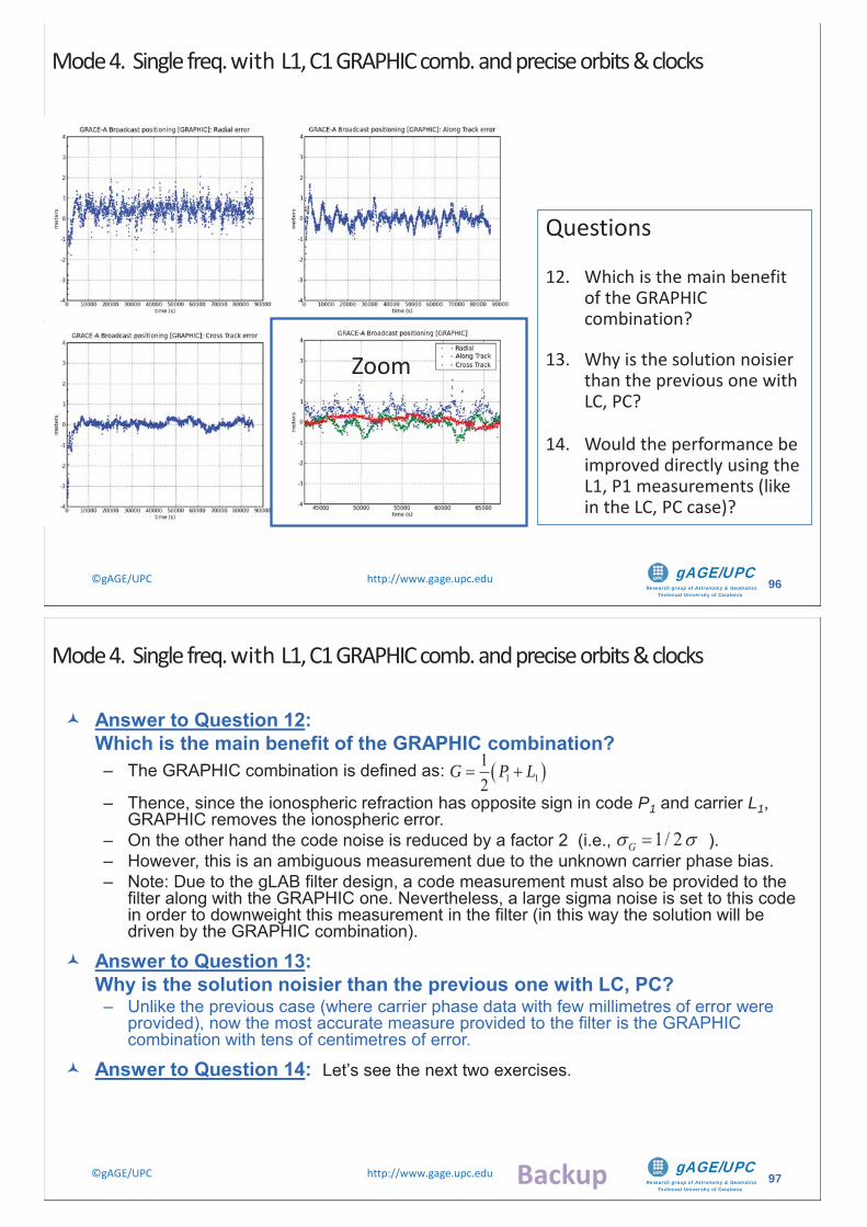
Research group of Astronomy & GeomaticsTechnical University of Catalonia
gAGE/UPC ©gAGE/UPC http://www.gage.upc.edu 96
Mode 4. Single freq. with L1, C1 GRAPHIC comb. and precise orbits & clocks
Questions
12. Which is the main benefit of the GRAPHIC combination?
13. Why is the solution noisier than the previous one with LC, PC?
14. Would the performance be improved directly using the L1, P1 measurements (like in the LC, PC case)?
Zoom
Research group of Astronomy & GeomaticsTechnical University of Catalonia
gAGE/UPC ©gAGE/UPC http://www.gage.upc.edu 97
Answer to Question 12: Which is the main benefit of the GRAPHIC combination?– The GRAPHIC combination is defined as:
– Thence, since the ionospheric refraction has opposite sign in code P1 and carrier L1, GRAPHIC removes the ionospheric error.
– On the other hand the code noise is reduced by a factor 2 (i.e., ).– However, this is an ambiguous measurement due to the unknown carrier phase bias.– Note: Due to the gLAB filter design, a code measurement must also be provided to the
filter along with the GRAPHIC one. Nevertheless, a large sigma noise is set to this code in order to downweight this measurement in the filter (in this way the solution will be driven by the GRAPHIC combination).
Answer to Question 13: Why is the solution noisier than the previous one with LC, PC?– Unlike the previous case (where carrier phase data with few millimetres of error were
provided), now the most accurate measure provided to the filter is the GRAPHIC combination with tens of centimetres of error.
Answer to Question 14: Let’s see the next two exercises.
1 112
G P L
1/ 2G
Mode 4. Single freq. with L1, C1 GRAPHIC comb. and precise orbits & clocks
Backup
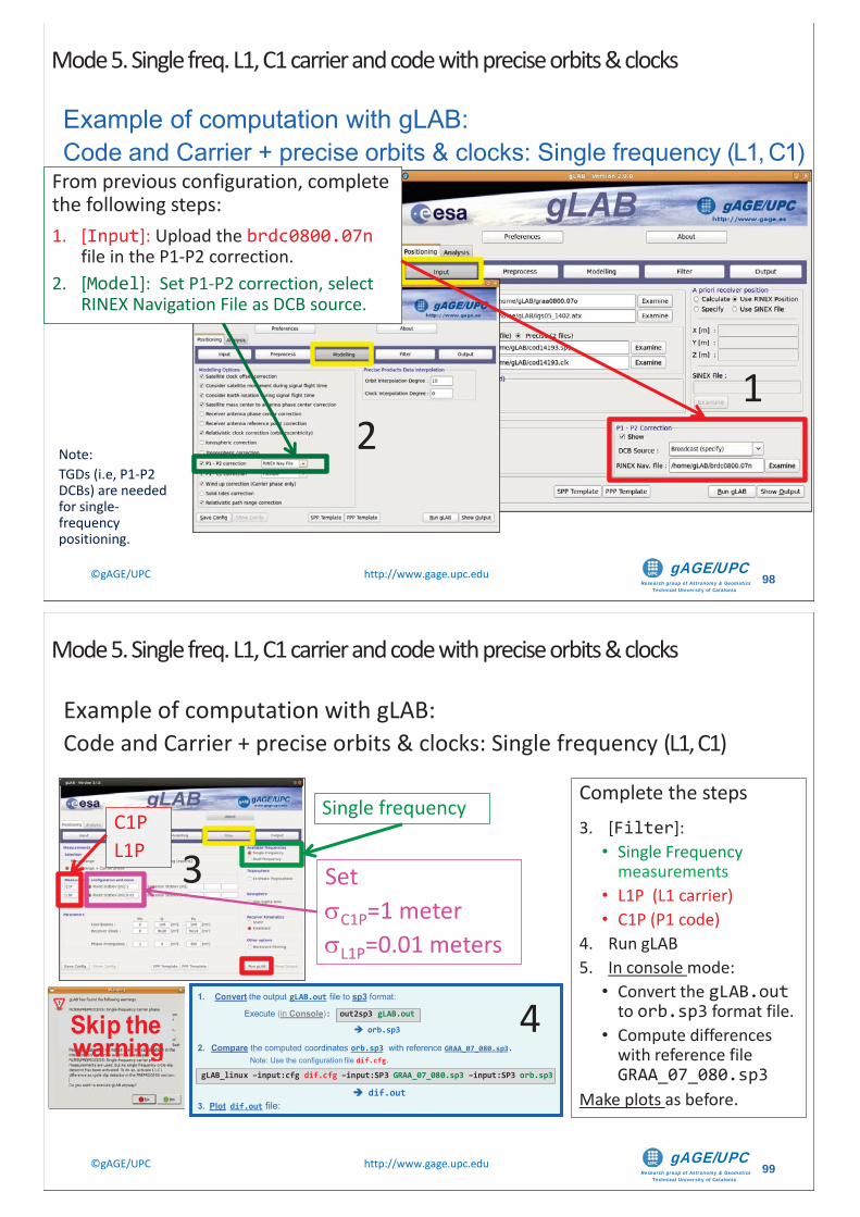
Research group of Astronomy & GeomaticsTechnical University of Catalonia
gAGE/UPC ©gAGE/UPC http://www.gage.upc.edu 98
Example of computation with gLAB: Code and Carrier + precise orbits & clocks: Single frequency (L1, C1)
Mode 5. Single freq. L1, C1 carrier and code with precise orbits & clocks
1
From previous configuration, complete the following steps:1. [Input]: Upload the brdc0800.07n
file in the P1-P2 correction.2. [Model]: Set P1-P2 correction, select
RINEX Navigation File as DCB source.
Note: TGDs (i.e, P1-P2 DCBs) are needed for single-frequency positioning.
21
Research group of Astronomy & GeomaticsTechnical University of Catalonia
gAGE/UPC ©gAGE/UPC http://www.gage.upc.edu 99
1. Convert the output gLAB.out file to sp3 format:
Execute (in Console): out2sp3 gLAB.out
orb.sp3
2. Compare the computed coordinates orb.sp3 with reference GRAA_07_080.sp3. Note: Use the configuration file dif.cfg.
gLAB_linux –input:cfg dif.cfg –input:SP3 GRAA_07_080.sp3 –input:SP3 orb.sp3
dif.out3. Plot dif.out file:
4
Complete the steps 3. [Filter]:
• Single Frequency measurements
• L1P (L1 carrier)• C1P (P1 code)
4. Run gLAB5. In console mode:
• Convert the gLAB.outto orb.sp3 format file.
• Compute differences with reference file GRAA_07_080.sp3
Make plots as before.
3C1PL1P
Single frequency
Set C1P=1 meterL1P=0.01 meters
Skip thewarning
Example of computation with gLAB: Code and Carrier + precise orbits & clocks: Single frequency (L1, C1)
Mode 5. Single freq. L1, C1 carrier and code with precise orbits & clocks
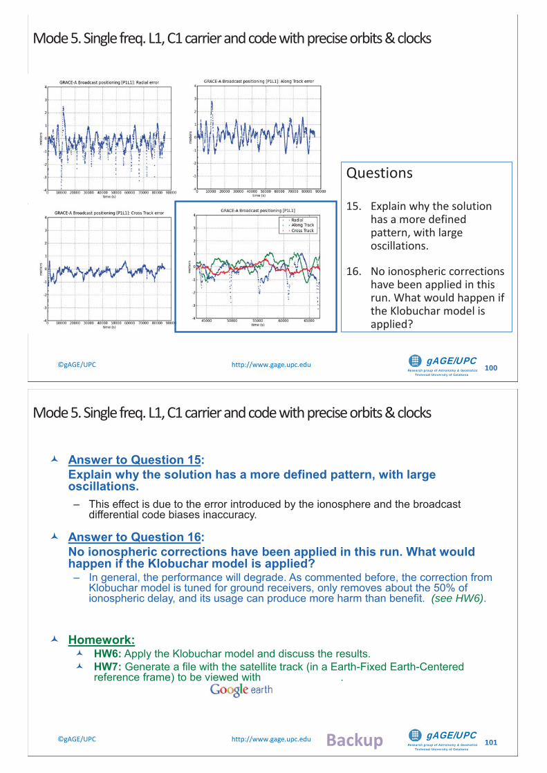
Research group of Astronomy & GeomaticsTechnical University of Catalonia
gAGE/UPC ©gAGE/UPC http://www.gage.upc.edu 100
Questions
15. Explain why the solution has a more defined pattern, with large oscillations.
16. No ionospheric corrections have been applied in this run. What would happen if the Klobuchar model is applied?
Mode 5. Single freq. L1, C1 carrier and code with precise orbits & clocks
Research group of Astronomy & GeomaticsTechnical University of Catalonia
gAGE/UPC ©gAGE/UPC http://www.gage.upc.edu 101
Answer to Question 15: Explain why the solution has a more defined pattern, with large oscillations.– This effect is due to the error introduced by the ionosphere and the broadcast
differential code biases inaccuracy.
Answer to Question 16: No ionospheric corrections have been applied in this run. What would happen if the Klobuchar model is applied?– In general, the performance will degrade. As commented before, the correction from
Klobuchar model is tuned for ground receivers, only removes about the 50% of ionospheric delay, and its usage can produce more harm than benefit. (see HW6).
Homework:HW6: Apply the Klobuchar model and discuss the results.HW7: Generate a file with the satellite track (in a Earth-Fixed Earth-Centeredreference frame) to be viewed with .
Mode 5. Single freq. L1, C1 carrier and code with precise orbits & clocks
Backup
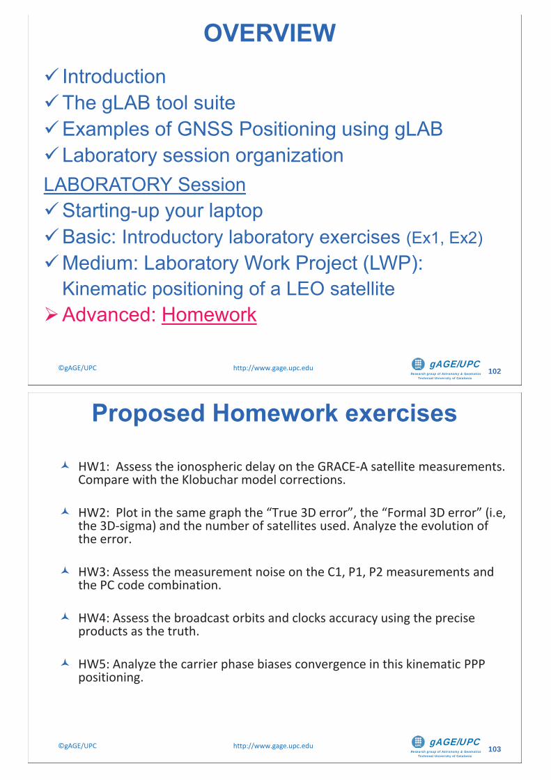
Research group of Astronomy & GeomaticsTechnical University of Catalonia
gAGE/UPC ©gAGE/UPC http://www.gage.upc.edu 102
IntroductionThe gLAB tool suiteExamples of GNSS Positioning using gLABLaboratory session organization
LABORATORY SessionStarting-up your laptopBasic: Introductory laboratory exercises (Ex1, Ex2)Medium: Laboratory Work Project (LWP): Kinematic positioning of a LEO satelliteAdvanced: Homework
OVERVIEW
Research group of Astronomy & GeomaticsTechnical University of Catalonia
gAGE/UPC ©gAGE/UPC http://www.gage.upc.edu 103
Proposed Homework exercises
HW1: Assess the ionospheric delay on the GRACE-A satellite measurements. Compare with the Klobuchar model corrections.
HW2: Plot in the same graph the “True 3D error”, the “Formal 3D error” (i.e, the 3D-sigma) and the number of satellites used. Analyze the evolution of the error.
HW3: Assess the measurement noise on the C1, P1, P2 measurements and the PC code combination.
HW4: Assess the broadcast orbits and clocks accuracy using the precise products as the truth.
HW5: Analyze the carrier phase biases convergence in this kinematic PPP positioning.
Research group of Astronomy & GeomaticsTechnical University of Catalonia
gAGE/UPC ©gAGE/UPC http://www.gage.upc.edu 104
HW6: Apply the Klobuchar model to the L1, P1 positioning with precise orbits and clocks and discuss the results.
HW7: Generate a file with the satellite track (in a Earth-Fixed Earth-Centeredreference frame) to be viewed with .
( ......
Proposed Homework exercises
Research group of Astronomy & GeomaticsTechnical University of Catalonia
gAGE/UPC ©gAGE/UPC http://www.gage.upc.edu 105
Backup slides
Homework help and answers

Research group of Astronomy & GeomaticsTechnical University of Catalonia
gAGE/UPC ©gAGE/UPC http://www.gage.upc.edu 106
Configure gLAB as in Mode 1 and complete the following steps:
1. [Output]: set • Print INPUT Message• Print MODEL Message (see message content in the Tooltips)
2. Run gLAB.
3. Make plots:[Analysis] section:• Click on the preconfigured Ionospheric
combinations option.• Complete the [Plot1, Plot2, Plot3] panels
configuration as indicated in the next slide.
Note: This configuration will provide:Plot 1: L1-L2 as a function of time for ALL sat.Plot 2: L1-L2 as a function of time for PRN16.Plot 3: P2-P1 as a function of time for PRN16
HW1: Assessing the ionospheric delay on the GRACE-A satellite
Backup
Research group of Astronomy & GeomaticsTechnical University of Catalonia
gAGE/UPC ©gAGE/UPC http://www.gage.upc.edu 107
$11-$12 L1-L2$10-$9 P2-P1
$11-$12 L1-L2
Plot 1
Plot 2
Plot 3
HW1: Assessing the ionospheric delay on the GRACE-A satellite
Note: This plot take some time to rise !
Backup
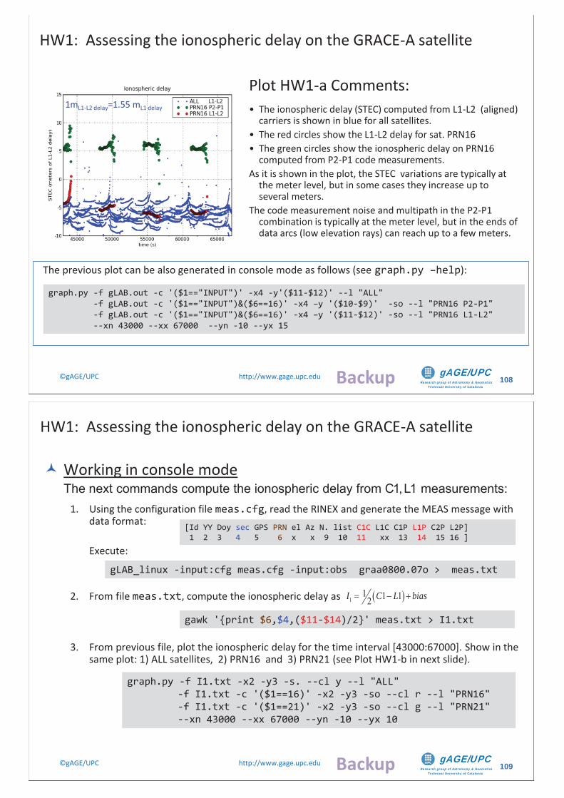
Research group of Astronomy & GeomaticsTechnical University of Catalonia
gAGE/UPC ©gAGE/UPC http://www.gage.upc.edu 108
graph.py -f gLAB.out -c '($1=="INPUT")' -x4 -y'($11-$12)' --l "ALL" -f gLAB.out -c '($1=="INPUT")&($6==16)' -x4 –y '($10-$9)' -so --l "PRN16 P2-P1" -f gLAB.out -c '($1=="INPUT")&($6==16)' -x4 –y '($11-$12)' -so --l "PRN16 L1-L2" --xn 43000 --xx 67000 --yn -10 --yx 15
Plot HW1-a Comments:• The ionospheric delay (STEC) computed from L1-L2 (aligned)
carriers is shown in blue for all satellites.• The red circles show the L1-L2 delay for sat. PRN16• The green circles show the ionospheric delay on PRN16
computed from P2-P1 code measurements.As it is shown in the plot, the STEC variations are typically at
the meter level, but in some cases they increase up to several meters.
The code measurement noise and multipath in the P2-P1 combination is typically at the meter level, but in the ends of data arcs (low elevation rays) can reach up to a few meters.
1mL1-L2 delay=1.55 mL1 delay
The previous plot can be also generated in console mode as follows (see graph.py –help):
HW1: Assessing the ionospheric delay on the GRACE-A satellite
Backup
Research group of Astronomy & GeomaticsTechnical University of Catalonia
gAGE/UPC ©gAGE/UPC http://www.gage.upc.edu 109
Working in console modeThe next commands compute the ionospheric delay from C1, L1 measurements:
1. Using the configuration file meas.cfg, read the RINEX and generate the MEAS message with data format:
Execute:
2. From file meas.txt, compute the ionospheric delay as
3. From previous file, plot the ionospheric delay for the time interval [43000:67000]. Show in the same plot: 1) ALL satellites, 2) PRN16 and 3) PRN21 (see Plot HW1-b in next slide).
graph.py -f I1.txt -x2 -y3 -s. --cl y --l "ALL" -f I1.txt -c '($1==16)' -x2 -y3 -so --cl r --l "PRN16" -f I1.txt -c '($1==21)' -x2 -y3 -so --cl g --l "PRN21" --xn 43000 --xx 67000 --yn -10 --yx 10
gLAB_linux -input:cfg meas.cfg -input:obs graa0800.07o > meas.txt
11 1 12I C L bias
gawk '{print $6,$4,($11-$14)/2}' meas.txt > I1.txt
HW1: Assessing the ionospheric delay on the GRACE-A satellite
[Id YY Doy sec GPS PRN el Az N. list C1C L1C C1P L1P C2P L2P]1 2 3 4 5 6 x x 9 10 11 xx 13 14 15 16 ]
Backup
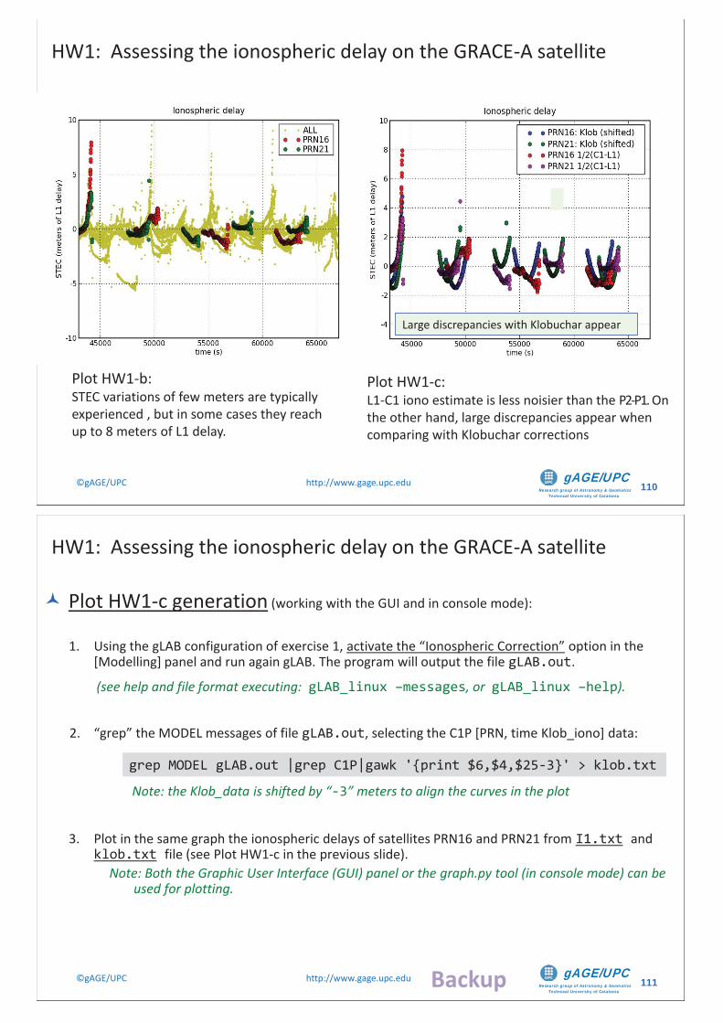
Research group of Astronomy & GeomaticsTechnical University of Catalonia
gAGE/UPC ©gAGE/UPC http://www.gage.upc.edu 110
Plot HW1-b: STEC variations of few meters are typically experienced , but in some cases they reach up to 8 meters of L1 delay.
Plot HW1-c: L1-C1 iono estimate is less noisier than the P2-P1. On the other hand, large discrepancies appear when comparing with Klobuchar corrections
Large discrepancies with Klobuchar appear
HW1: Assessing the ionospheric delay on the GRACE-A satellite
Research group of Astronomy & GeomaticsTechnical University of Catalonia
gAGE/UPC ©gAGE/UPC http://www.gage.upc.edu 111
Plot HW1-c generation (working with the GUI and in console mode):
1. Using the gLAB configuration of exercise 1, activate the “Ionospheric Correction” option in the [Modelling] panel and run again gLAB. The program will output the file gLAB.out.
(see help and file format executing: gLAB_linux –messages, or gLAB_linux –help).
2. “grep” the MODEL messages of file gLAB.out, selecting the C1P [PRN, time Klob_iono] data:
Note: the Klob_data is shifted by “-3” meters to align the curves in the plot
3. Plot in the same graph the ionospheric delays of satellites PRN16 and PRN21 from I1.txt and klob.txt file (see Plot HW1-c in the previous slide).
Note: Both the Graphic User Interface (GUI) panel or the graph.py tool (in console mode) can beused for plotting.
grep MODEL gLAB.out |grep C1P|gawk '{print $6,$4,$25-3}' > klob.txt
HW1: Assessing the ionospheric delay on the GRACE-A satellite
Backup
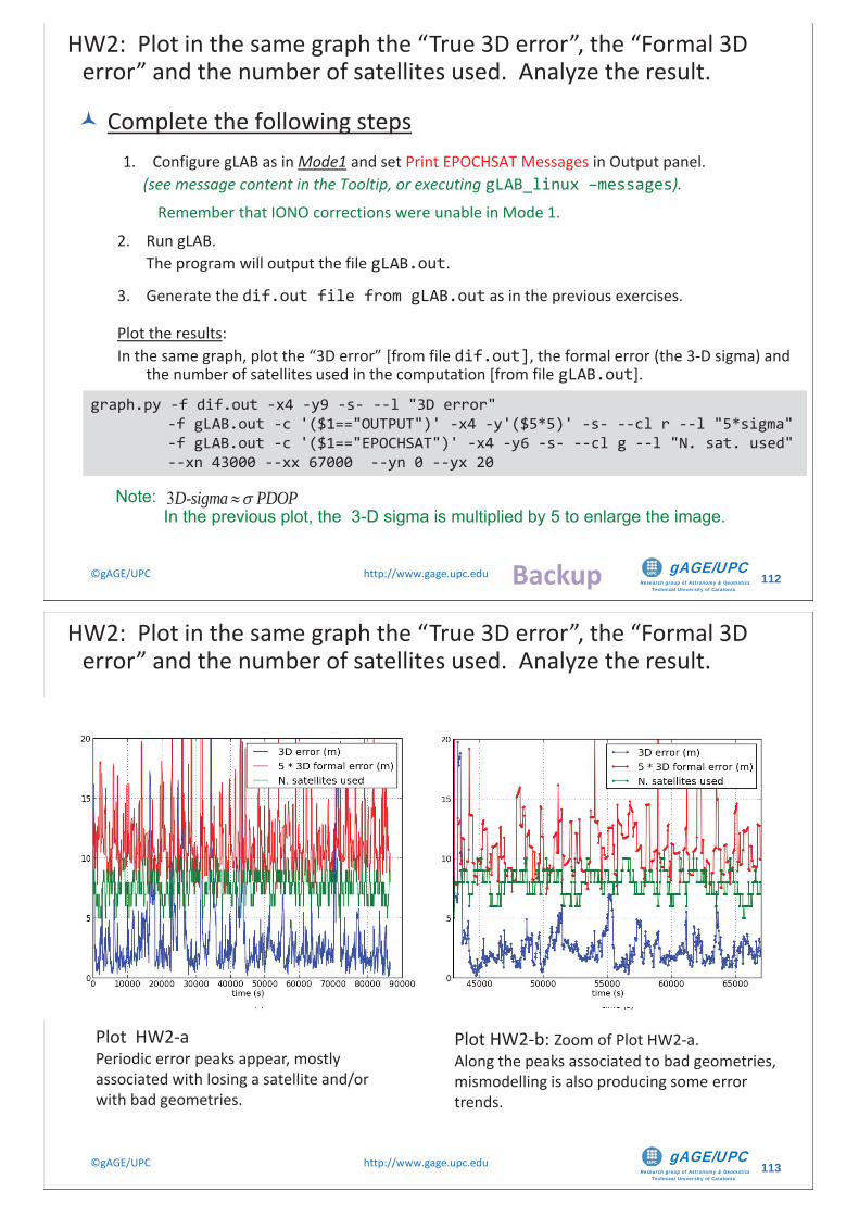
Research group of Astronomy & GeomaticsTechnical University of Catalonia
gAGE/UPC ©gAGE/UPC http://www.gage.upc.edu 112
Complete the following steps1. Configure gLAB as in Mode1 and set Print EPOCHSAT Messages in Output panel.
(see message content in the Tooltip, or executing gLAB_linux –messages).
Remember that IONO corrections were unable in Mode 1.
2. Run gLAB.The program will output the file gLAB.out.
3. Generate the dif.out file from gLAB.out as in the previous exercises.
Plot the results: In the same graph, plot the “3D error” [from file dif.out], the formal error (the 3-D sigma) and
the number of satellites used in the computation [from file gLAB.out].
graph.py -f dif.out -x4 -y9 -s- --l "3D error" -f gLAB.out -c '($1=="OUTPUT")' -x4 -y'($5*5)' -s- --cl r --l "5*sigma" -f gLAB.out -c '($1=="EPOCHSAT")' -x4 -y6 -s- --cl g --l "N. sat. used" --xn 43000 --xx 67000 --yn 0 --yx 20
HW2: Plot in the same graph the “True 3D error”, the “Formal 3D error” and the number of satellites used. Analyze the result.
Note:In the previous plot, the 3-D sigma is multiplied by 5 to enlarge the image.3 -D sigma PDOP
Backup
Research group of Astronomy & GeomaticsTechnical University of Catalonia
gAGE/UPC ©gAGE/UPC http://www.gage.upc.edu 113
Large discrepancies with Klobuchar appearSTEC variations of few meters, but in somecases, reaching up to 8 meters of L1 delay.
Plot HW2-aPeriodic error peaks appear, mostly associated with losing a satellite and/or with bad geometries.
Plot HW2-b: Zoom of Plot HW2-a. Along the peaks associated to bad geometries, mismodelling is also producing some error trends.
HW2: Plot in the same graph the “True 3D error”, the “Formal 3D error” and the number of satellites used. Analyze the result.
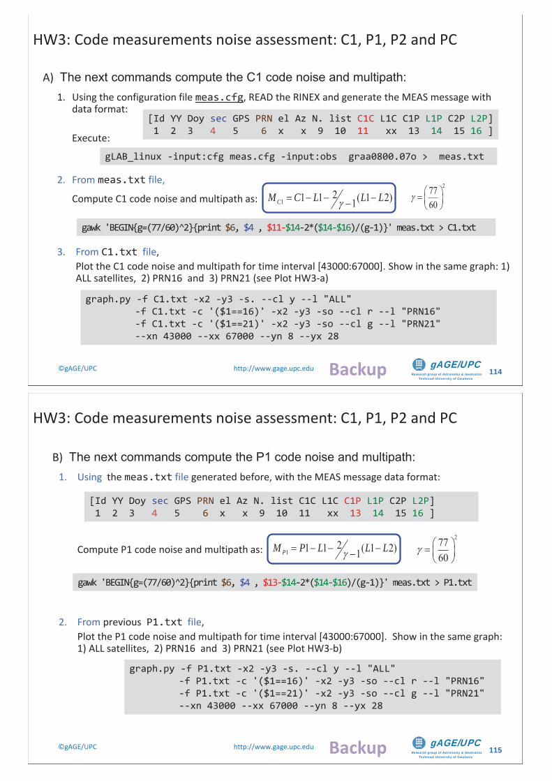
Research group of Astronomy & GeomaticsTechnical University of Catalonia
gAGE/UPC ©gAGE/UPC http://www.gage.upc.edu 114
A) The next commands compute the C1 code noise and multipath:1. Using the configuration file meas.cfg, READ the RINEX and generate the MEAS message with
data format:
Execute:
2. From meas.txt file,
Compute C1 code noise and multipath as:
3. From C1.txt file, Plot the C1 code noise and multipath for time interval [43000:67000]. Show in the same graph: 1) ALL satellites, 2) PRN16 and 3) PRN21 (see Plot HW3-a)
graph.py -f C1.txt -x2 -y3 -s. --cl y --l "ALL" -f C1.txt -c '($1==16)' -x2 -y3 -so --cl r --l "PRN16" -f C1.txt -c '($1==21)' -x2 -y3 -so --cl g --l "PRN21" --xn 43000 --xx 67000 --yn 8 --yx 28
[Id YY Doy sec GPS PRN el Az N. list C1C L1C C1P L1P C2P L2P]1 2 3 4 5 6 x x 9 10 11 xx 13 14 15 16 ]
gLAB_linux -input:cfg meas.cfg -input:obs graa0800.07o > meas.txt
gawk 'BEGIN{g=(77/60) 2}{print $6, $4 , $11-$14-2*($14-$16)/(g-1)}' meas.txt > C1.txt
HW3: Code measurements noise assessment: C1, P1, P2 and PC
121 1 ( 1 2)1CM C L L L
27760
Backup
Research group of Astronomy & GeomaticsTechnical University of Catalonia
gAGE/UPC ©gAGE/UPC http://www.gage.upc.edu 115
B) The next commands compute the P1 code noise and multipath:1. Using the meas.txt file generated before, with the MEAS message data format:
Compute P1 code noise and multipath as:
2. From previous P1.txt file, Plot the P1 code noise and multipath for time interval [43000:67000]. Show in the same graph: 1) ALL satellites, 2) PRN16 and 3) PRN21 (see Plot HW3-b)
graph.py -f P1.txt -x2 -y3 -s. --cl y --l "ALL" -f P1.txt -c '($1==16)' -x2 -y3 -so --cl r --l "PRN16" -f P1.txt -c '($1==21)' -x2 -y3 -so --cl g --l "PRN21" --xn 43000 --xx 67000 --yn 8 --yx 28
[Id YY Doy sec GPS PRN el Az N. list C1C L1C C1P L1P C2P L2P]1 2 3 4 5 6 x x 9 10 11 xx 13 14 15 16 ]
gawk 'BEGIN{g=(77/60) 2}{print $6, $4 , $13-$14-2*($14-$16)/(g-1)}' meas.txt > P1.txt
121 1 ( 1 2)1PM P L L L
27760
HW3: Code measurements noise assessment: C1, P1, P2 and PC
Backup
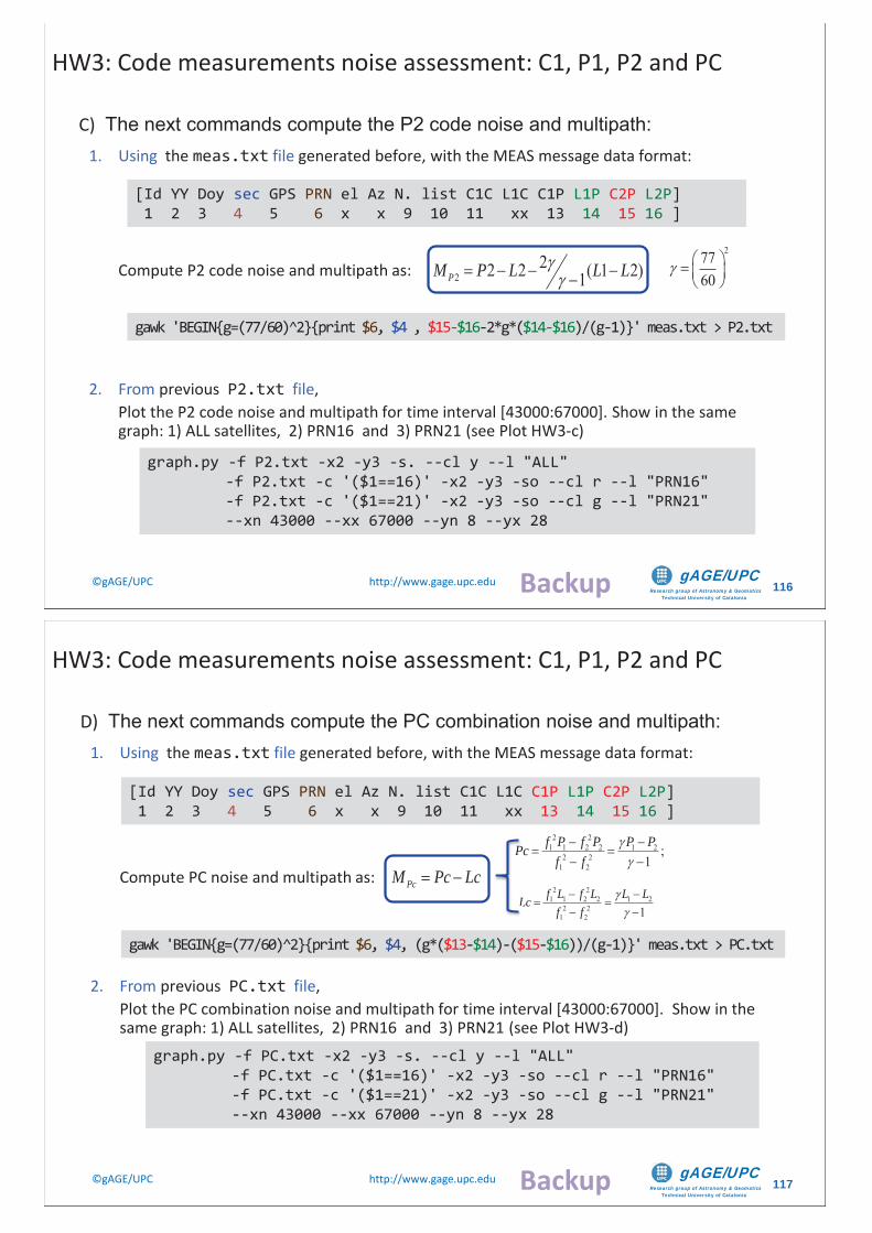
Research group of Astronomy & GeomaticsTechnical University of Catalonia
gAGE/UPC ©gAGE/UPC http://www.gage.upc.edu 116
C) The next commands compute the P2 code noise and multipath:1. Using the meas.txt file generated before, with the MEAS message data format:
Compute P2 code noise and multipath as:
2. From previous P2.txt file, Plot the P2 code noise and multipath for time interval [43000:67000]. Show in the same graph: 1) ALL satellites, 2) PRN16 and 3) PRN21 (see Plot HW3-c)
graph.py -f P2.txt -x2 -y3 -s. --cl y --l "ALL" -f P2.txt -c '($1==16)' -x2 -y3 -so --cl r --l "PRN16" -f P2.txt -c '($1==21)' -x2 -y3 -so --cl g --l "PRN21" --xn 43000 --xx 67000 --yn 8 --yx 28
[Id YY Doy sec GPS PRN el Az N. list C1C L1C C1P L1P C2P L2P]1 2 3 4 5 6 x x 9 10 11 xx 13 14 15 16 ]
gawk 'BEGIN{g=(77/60) 2}{print $6, $4 , $15-$16-2*g*($14-$16)/(g-1)}' meas.txt > P2.txt
222 2 ( 1 2)1PM P L L L
27760
HW3: Code measurements noise assessment: C1, P1, P2 and PC
Backup
Research group of Astronomy & GeomaticsTechnical University of Catalonia
gAGE/UPC ©gAGE/UPC http://www.gage.upc.edu 117
D) The next commands compute the PC combination noise and multipath:1. Using the meas.txt file generated before, with the MEAS message data format:
Compute PC noise and multipath as:
2. From previous PC.txt file, Plot the PC combination noise and multipath for time interval [43000:67000]. Show in the same graph: 1) ALL satellites, 2) PRN16 and 3) PRN21 (see Plot HW3-d)
graph.py -f PC.txt -x2 -y3 -s. --cl y --l "ALL" -f PC.txt -c '($1==16)' -x2 -y3 -so --cl r --l "PRN16" -f PC.txt -c '($1==21)' -x2 -y3 -so --cl g --l "PRN21" --xn 43000 --xx 67000 --yn 8 --yx 28
[Id YY Doy sec GPS PRN el Az N. list C1C L1C C1P L1P C2P L2P]1 2 3 4 5 6 x x 9 10 11 xx 13 14 15 16 ]
PcM Pc Lc2 21 1 2 2 1 2
2 21 2 1
f L f L L LLcf f
gawk 'BEGIN{g=(77/60) 2}{print $6, $4, (g*($13-$14)-($15-$16))/(g-1)}' meas.txt > PC.txt
HW3: Code measurements noise assessment: C1, P1, P2 and PC
2 21 1 2 2 1 2
2 21 2
;1
f P f P P PPcf f
L
P
Backup
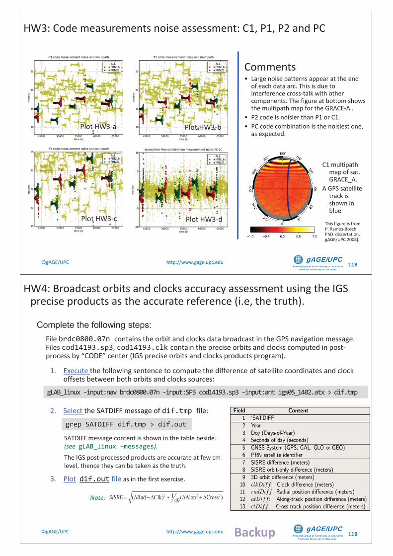
Research group of Astronomy & GeomaticsTechnical University of Catalonia
gAGE/UPC ©gAGE/UPC http://www.gage.upc.edu 118
Comments• Large noise patterns appear at the end
of each data arc. This is due to interference cross-talk with other components. The figure at bottom shows the multipath map for the GRACE-A .
• P2 code is noisier than P1 or C1.• PC code combination is the noisiest one,
as expected.
C1 multipath map of sat. GRACE_A.
A GPS satellite track is shown in blue
This figure is from P. Ramos-Bosch PhD dissertation, gAGE/UPC 2008].
Plot HW3-a Plot HW3-b
Plot HW3-c Plot HW3-d
HW3: Code measurements noise assessment: C1, P1, P2 and PC
Research group of Astronomy & GeomaticsTechnical University of Catalonia
gAGE/UPC ©gAGE/UPC http://www.gage.upc.edu 119
Complete the following steps:File brdc0800.07n contains the orbit and clocks data broadcast in the GPS navigation message. Files cod14193.sp3, cod14193.clk contain the precise orbits and clocks computed in post-process by “CODE” center (IGS precise orbits and clocks products program).
1. Execute the following sentence to compute the difference of satellite coordinates and clock offsets between both orbits and clocks sources:
2. Select the SATDIFF message of dif.tmp file:
3. Plot dif.out file as in the first exercise.
Note:
gLAB_linux -input:nav brdc0800.07n -input:SP3 cod14193.sp3 -input:ant igs05_1402.atx > dif.tmp
HW4: Broadcast orbits and clocks accuracy assessment using the IGS precise products as the accurate reference (i.e, the truth).
grep SATDIFF dif.tmp > dif.out
SATDIFF message content is shown in the table beside.(see gLAB_linux –messages).The IGS post-processed products are accurate at few cm level, thence they can be taken as the truth.
2 2 21( Rad Clk) ( Alon Cross )49SISRE
Backup
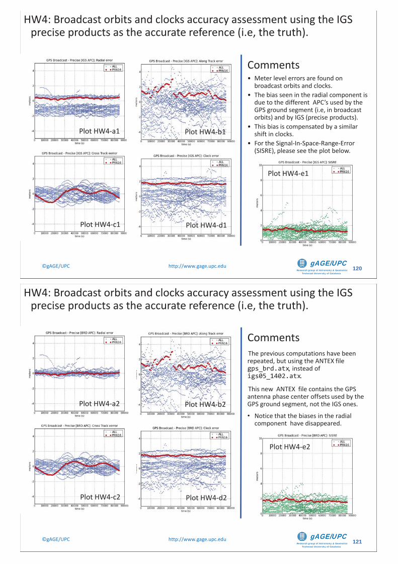
Research group of Astronomy & GeomaticsTechnical University of Catalonia
gAGE/UPC ©gAGE/UPC http://www.gage.upc.edu 120
Comments• Meter level errors are found on
broadcast orbits and clocks.• The bias seen in the radial component is
due to the different APC’s used by the GPS ground segment (i.e, in broadcast orbits) and by IGS (precise products).
• This bias is compensated by a similar shift in clocks.
• For the Signal-In-Space-Range-Error (SISRE), please see the plot below.
Plot HW4-a1 Plot HW4-b1
Plot HW4-c1 Plot HW4-d1
Plot HW4-e1
HW4: Broadcast orbits and clocks accuracy assessment using the IGS precise products as the accurate reference (i.e, the truth).
Research group of Astronomy & GeomaticsTechnical University of Catalonia
gAGE/UPC ©gAGE/UPC http://www.gage.upc.edu 121
CommentsThe previous computations have been repeated, but using the ANTEX file gps_brd.atx, instead of igs05_1402.atx.
This new ANTEX file contains the GPS antenna phase center offsets used by the GPS ground segment, not the IGS ones.
• Notice that the biases in the radial component have disappeared.
Plot HW4-a2 Plot HW4-b2
Plot HW4-c2 Plot HW4-d2
Plot HW4-e2
HW4: Broadcast orbits and clocks accuracy assessment using the IGS precise products as the accurate reference (i.e, the truth).
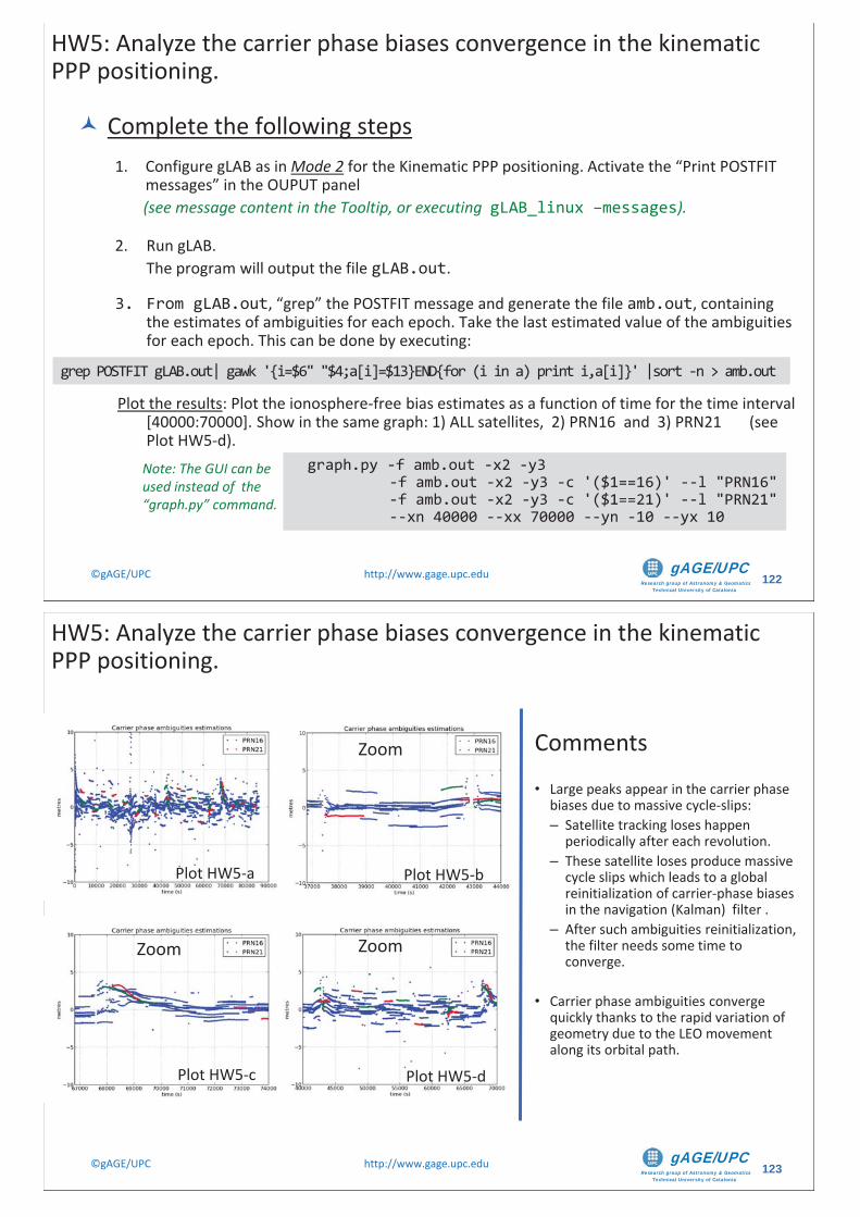
Research group of Astronomy & GeomaticsTechnical University of Catalonia
gAGE/UPC ©gAGE/UPC http://www.gage.upc.edu 122
HW5: Analyze the carrier phase biases convergence in the kinematic PPP positioning.
Plot the results: Plot the ionosphere-free bias estimates as a function of time for the time interval [40000:70000]. Show in the same graph: 1) ALL satellites, 2) PRN16 and 3) PRN21 (see Plot HW5-d).
grep POSTFIT gLAB.out| gawk '{i=$6" "$4;a[i]=$13}END{for (i in a) print i,a[i]}' |sort -n > amb.out
graph.py -f amb.out -x2 -y3 -f amb.out -x2 -y3 -c '($1==16)' --l "PRN16" -f amb.out -x2 -y3 -c '($1==21)' --l "PRN21" --xn 40000 --xx 70000 --yn -10 --yx 10
Note: The GUI can be used instead of the “graph.py” command.
Complete the following steps1. Configure gLAB as in Mode 2 for the Kinematic PPP positioning. Activate the “Print POSTFIT
messages” in the OUPUT panel(see message content in the Tooltip, or executing gLAB_linux –messages).
2. Run gLAB.The program will output the file gLAB.out.
3. From gLAB.out, “grep” the POSTFIT message and generate the file amb.out, containing the estimates of ambiguities for each epoch. Take the last estimated value of the ambiguities for each epoch. This can be done by executing:
Research group of Astronomy & GeomaticsTechnical University of Catalonia
gAGE/UPC ©gAGE/UPC http://www.gage.upc.edu 123
Comments
• Large peaks appear in the carrier phase biases due to massive cycle-slips: – Satellite tracking loses happen
periodically after each revolution.– These satellite loses produce massive
cycle slips which leads to a global reinitialization of carrier-phase biases in the navigation (Kalman) filter .
– After such ambiguities reinitialization, the filter needs some time to converge.
• Carrier phase ambiguities converge quickly thanks to the rapid variation of geometry due to the LEO movement along its orbital path.
Plot HW5-a Plot HW5-b
Plot HW5-c Plot HW5-d
Zoom
ZoomZoom
HW5: Analyze the carrier phase biases convergence in the kinematic PPP positioning.
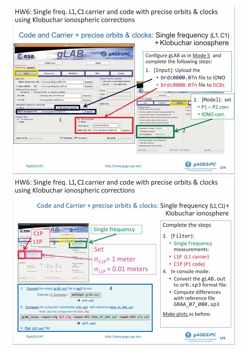
Research group of Astronomy & GeomaticsTechnical University of Catalonia
gAGE/UPC ©gAGE/UPC http://www.gage.upc.edu 124
Code and Carrier + precise orbits & clocks: Single frequency (L1, C1) + Klobuchar ionosphere
1
Configure gLAB as in Mode 5 and complete the following steps:1. [Input]: Upload the
• brdc0800.07n file to IONO• brdc0800.07n file to DCBs
2
2. [Model]: set• P1 – P2 corr.• IONO corr.
HW6: Single freq. L1, C1 carrier and code with precise orbits & clocks using Klobuchar ionospheric corrections
Research group of Astronomy & GeomaticsTechnical University of Catalonia
gAGE/UPC ©gAGE/UPC http://www.gage.upc.edu 125
1. Convert the output gLAB.out file to sp3 format:
Execute (in Console): out2sp3 gLAB.out
orb.sp3
2. Compare the computed coordinates orb.sp3 with reference GRAA_07_080.sp3. Note: Use the configuration file dif.cfg.
gLAB_linux –input:cfg dif.cfg –input:SP3 GRAA_07_080.sp3 –input:SP3 orb.sp3
dif.out3. Plot dif.out file:
4
Complete the steps
3. [Filter]:• Single Frequency
measurements:• L1P (L1 carrier)• C1P (P1 code)
4. In console mode:• Convert the gLAB.out
to orb.sp3 format file.• Compute differences
with reference file GRAA_07_080.sp3
Make plots as before.
3
C1PL1P
Single frequency
Set C1P= 1 meterL1P = 0.01 meters
HW6: Single freq. L1, C1 carrier and code with precise orbits & clocks using Klobuchar ionospheric corrections
Code and Carrier + precise orbits & clocks: Single frequency (L1, C1) + Klobuchar ionosphere
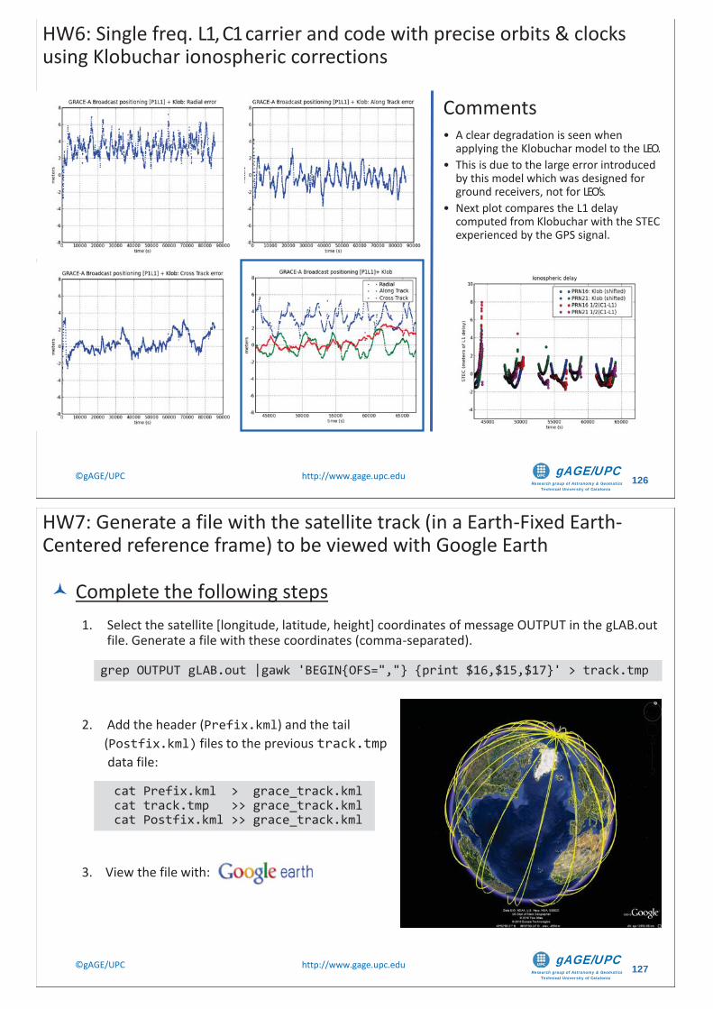
Research group of Astronomy & GeomaticsTechnical University of Catalonia
gAGE/UPC ©gAGE/UPC http://www.gage.upc.edu 126
Comments• A clear degradation is seen when
applying the Klobuchar model to the LEO.• This is due to the large error introduced
by this model which was designed for ground receivers, not for LEO’s.
• Next plot compares the L1 delay computed from Klobuchar with the STEC experienced by the GPS signal.
HW6: Single freq. L1, C1 carrier and code with precise orbits & clocks using Klobuchar ionospheric corrections
Research group of Astronomy & GeomaticsTechnical University of Catalonia
gAGE/UPC ©gAGE/UPC http://www.gage.upc.edu 127
HW7: Generate a file with the satellite track (in a Earth-Fixed Earth-Centered reference frame) to be viewed with Google Earth
Complete the following steps1. Select the satellite [longitude, latitude, height] coordinates of message OUTPUT in the gLAB.out
file. Generate a file with these coordinates (comma-separated).
2. Add the header (Prefix.kml) and the tail (Postfix.kml) files to the previous track.tmpdata file:
3. View the file with:
grep OUTPUT gLAB.out |gawk 'BEGIN{OFS=","} {print $16,$15,$17}' > track.tmp
cat Prefix.kml > grace_track.kmlcat track.tmp >> grace_track.kmlcat Postfix.kml >> grace_track.kml
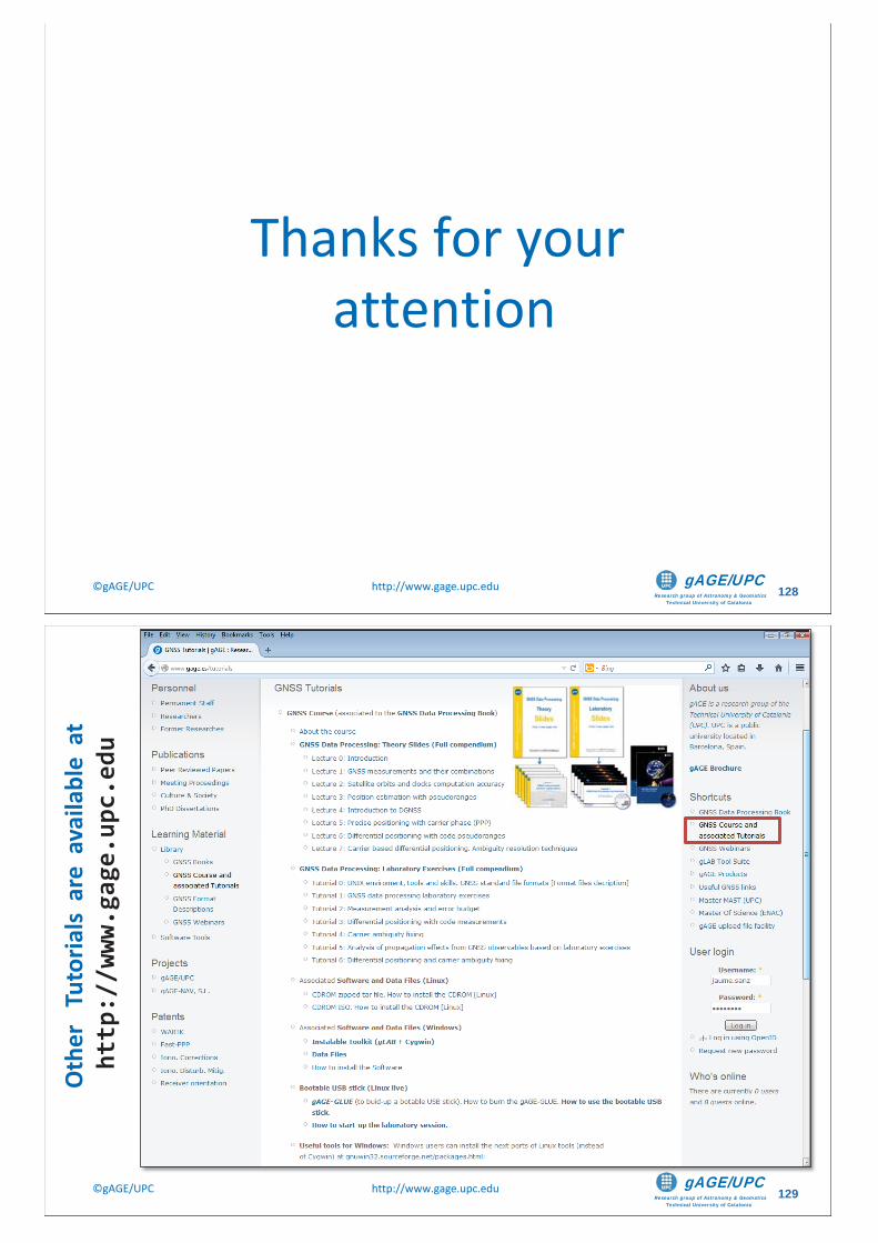
Research group of Astronomy & GeomaticsTechnical University of Catalonia
gAGE/UPC ©gAGE/UPC http://www.gage.upc.edu 128
Thanks for yourattention
Research group of Astronomy & GeomaticsTechnical University of Catalonia
gAGE/UPC ©gAGE/UPC http://www.gage.upc.edu 129
Oth
er
Tuto
rials
are
ava
ilabl
e a
t ht
tp:/
/www
.gag
e.up
c.ed
u
Research group of Astronomy & GeomaticsTechnical University of Catalonia
gAGE/UPC ©gAGE/UPC http://www.gage.upc.edu 130
• The ESA/UPC GNSS-Lab Tool suit (gLAB) has been developed under the ESA Education Office contract N. P1081434.
• The data set of GRACE-A LEO satellite was obtained from the NASA Physical Oceanography Distributed Active Archive Center at the Jet Propulsion Laboratory, California Institute of Technology.
• The other data files used in this study were acquired as part of NASA's Earth Science Data Systems and archived and distributed by the Crustal Dynamics Data Information System (CDDIS).
• To Pere Ramos-Bosch for his fully and generous disposition to perform gLAB updates in his afterhours.
• To Adrià Rovira-Garcia for his contribution to the edition of this material and gLAB updating.
• To Deimos Ibáñez for his contribution to gLAB updating and making the Windows installable version for this tutorial.
Acknowledgements

Research group of Astronomy & GeomaticsTechnical University of Catalonia
gAGE/UPC @ J. Sanz & J.M. Juan 1
Tutorial 2Measurements analysis
and error budget
Contact: [email protected] site: http://www.gage.upc.edu
Slides associated to gLAB version 2.0.0
Research group of Astronomy & GeomaticsTechnical University of Catalonia
gAGE/UPC @ J. Sanz & J.M. Juan 2
Authorship statement
The authorship of this material and the Intellectual Property Rights are owned by J. Sanz Subirana and J.M. Juan Zornoza.
These slides can be obtained either from the server http://www.gage.upc.edu,or [email protected]. Any partial reproduction should be previously authorized by the authors, clearly referring to the slides used.
This authorship statement must be kept intact and unchanged at all times.
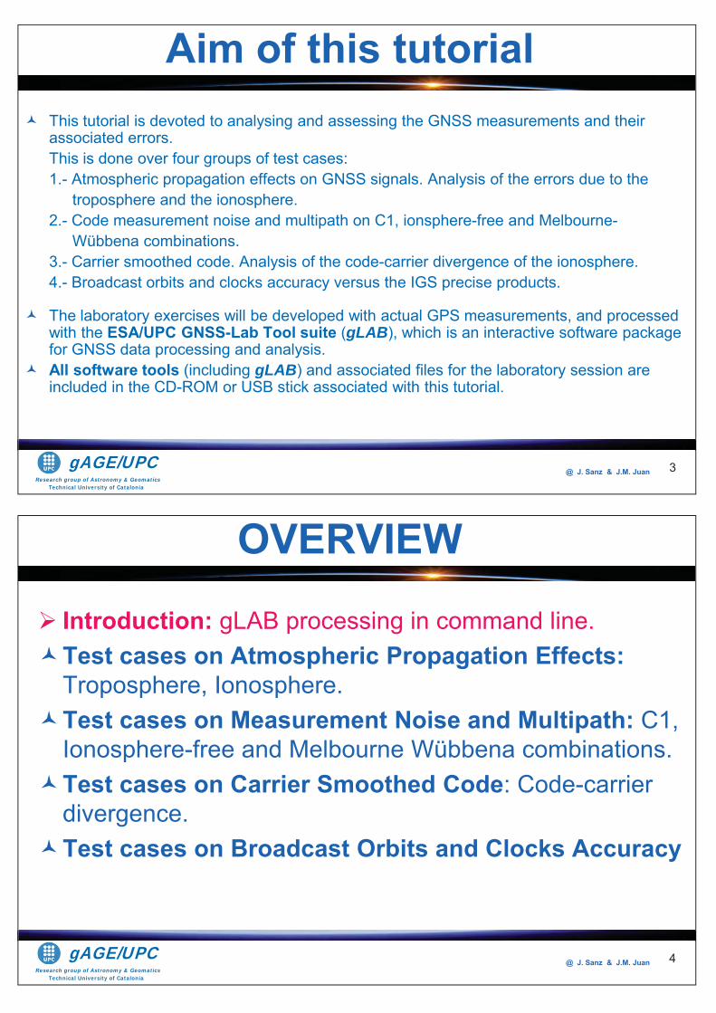
Research group of Astronomy & GeomaticsTechnical University of Catalonia
gAGE/UPC @ J. Sanz & J.M. Juan 3
This tutorial is devoted to analysing and assessing the GNSS measurements and their associated errors. This is done over four groups of test cases: 1.- Atmospheric propagation effects on GNSS signals. Analysis of the errors due to the
troposphere and the ionosphere.2.- Code measurement noise and multipath on C1, ionsphere-free and Melbourne-
Wübbena combinations.3.- Carrier smoothed code. Analysis of the code-carrier divergence of the ionosphere.4.- Broadcast orbits and clocks accuracy versus the IGS precise products.
The laboratory exercises will be developed with actual GPS measurements, and processed with the ESA/UPC GNSS-Lab Tool suite (gLAB), which is an interactive software package for GNSS data processing and analysis. All software tools (including gLAB) and associated files for the laboratory session are included in the CD-ROM or USB stick associated with this tutorial.
Aim of this tutorial
Research group of Astronomy & GeomaticsTechnical University of Catalonia
gAGE/UPC @ J. Sanz & J.M. Juan
Introduction: gLAB processing in command line.Test cases on Atmospheric Propagation Effects:Troposphere, Ionosphere. Test cases on Measurement Noise and Multipath: C1, Ionosphere-free and Melbourne Wübbena combinations.Test cases on Carrier Smoothed Code: Code-carrier divergence.Test cases on Broadcast Orbits and Clocks Accuracy
OVERVIEW
4
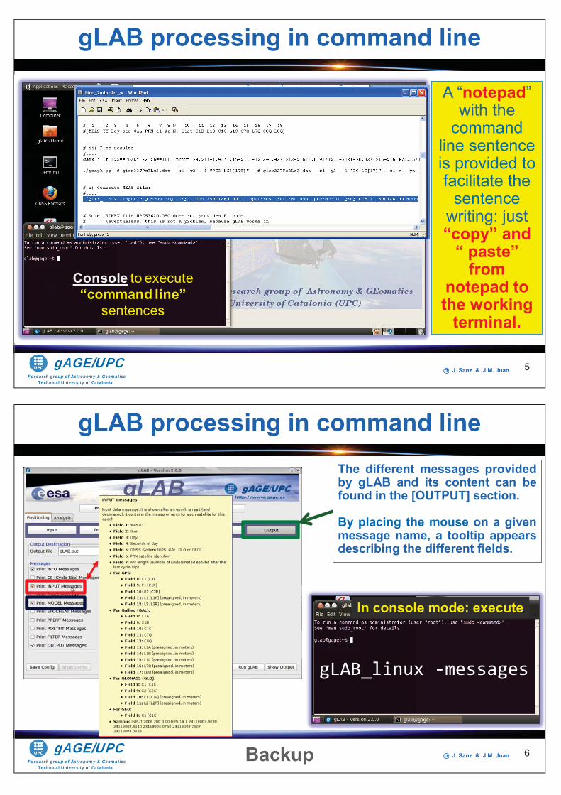
Research group of Astronomy & GeomaticsTechnical University of Catalonia
gAGE/UPC @ J. Sanz & J.M. Juan 5
Console to execute “command line”
sentences
A “notepad”with the
command line sentence is provided to facilitate the
sentence writing: just “copy” and
“ paste” from
notepad to the working
terminal.
gLAB processing in command line
Research group of Astronomy & GeomaticsTechnical University of Catalonia
gAGE/UPC @ J. Sanz & J.M. Juan 6
The different messages providedby gLAB and its content can befound in the [OUTPUT] section.
By placing the mouse on a givenmessage name, a tooltip appearsdescribing the different fields.
Backup
gLAB_linux -messages
In console mode: execute
gLAB processing in command line
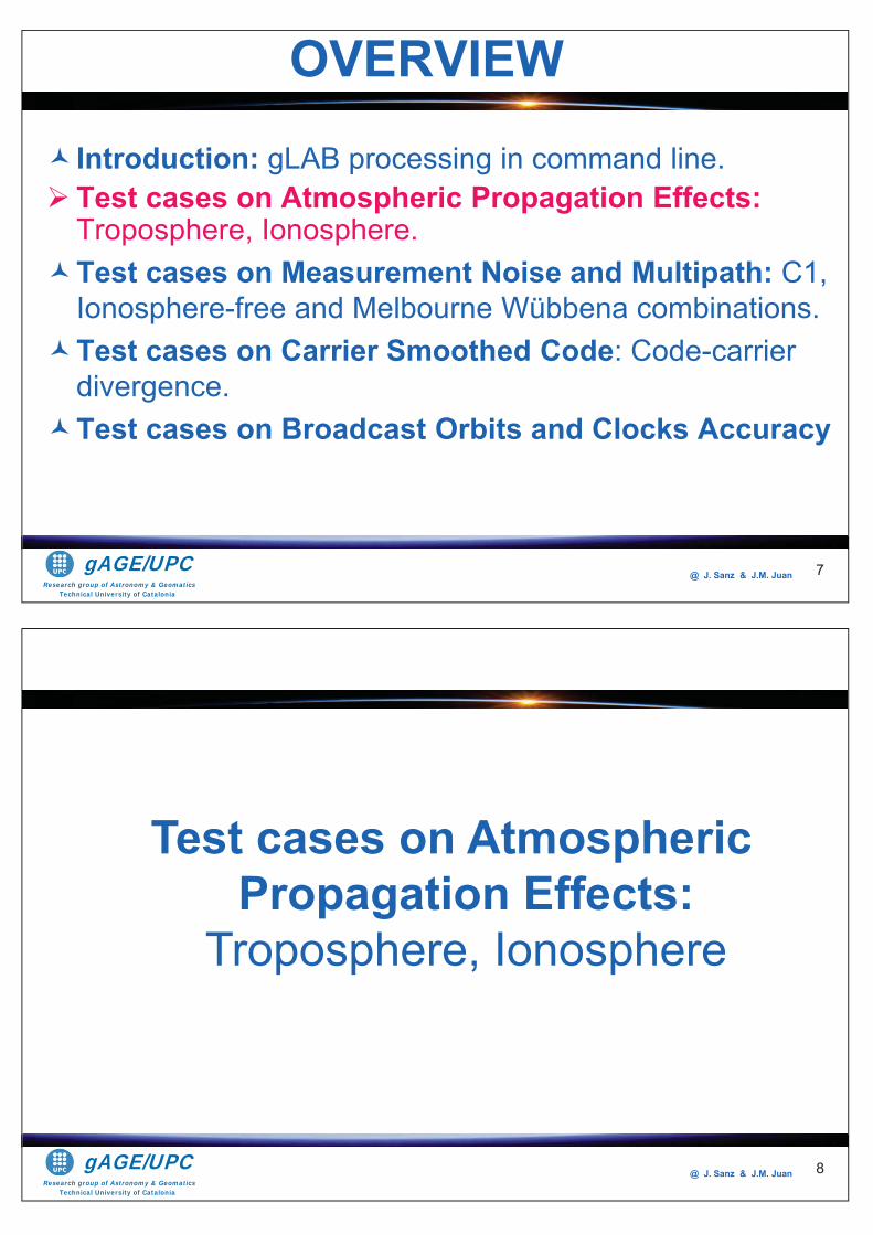
Research group of Astronomy & GeomaticsTechnical University of Catalonia
gAGE/UPC @ J. Sanz & J.M. Juan
Introduction: gLAB processing in command line.Test cases on Atmospheric Propagation Effects: Troposphere, Ionosphere.Test cases on Measurement Noise and Multipath: C1, Ionosphere-free and Melbourne Wübbena combinations.Test cases on Carrier Smoothed Code: Code-carrier divergence.Test cases on Broadcast Orbits and Clocks Accuracy
OVERVIEW
7
Research group of Astronomy & GeomaticsTechnical University of Catalonia
gAGE/UPC @ J. Sanz & J.M. Juan 8
Test cases on Atmospheric Propagation Effects:
Troposphere, Ionosphere
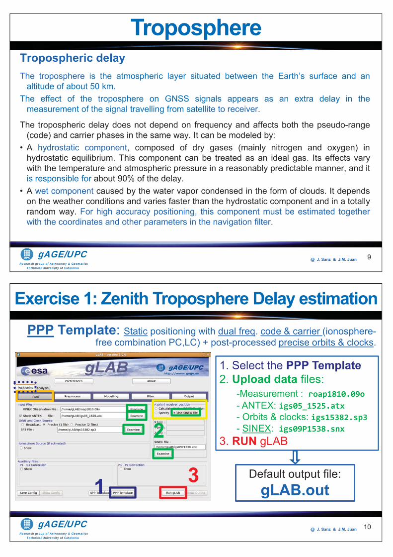
Research group of Astronomy & GeomaticsTechnical University of Catalonia
gAGE/UPC @ J. Sanz & J.M. Juan
Tropospheric delayThe troposphere is the atmospheric layer situated between the Earth’s surface and an
altitude of about 50 km.The effect of the troposphere on GNSS signals appears as an extra delay in the
measurement of the signal travelling from satellite to receiver.
The tropospheric delay does not depend on frequency and affects both the pseudo-range(code) and carrier phases in the same way. It can be modeled by:
• A hydrostatic component, composed of dry gases (mainly nitrogen and oxygen) inhydrostatic equilibrium. This component can be treated as an ideal gas. Its effects varywith the temperature and atmospheric pressure in a reasonably predictable manner, and itis responsible for about 90% of the delay.
• A wet component caused by the water vapor condensed in the form of clouds. It dependson the weather conditions and varies faster than the hydrostatic component and in a totallyrandom way. For high accuracy positioning, this component must be estimated togetherwith the coordinates and other parameters in the navigation filter.
9
Troposphere
Research group of Astronomy & GeomaticsTechnical University of Catalonia
gAGE/UPC @ J. Sanz & J.M. Juan
PPP Template: Static positioning with dual freq. code & carrier (ionosphere-free combination PC,LC) + post-processed precise orbits & clocks.
1. Select the PPP Template 2. Upload data files:
-Measurement : roap1810.09o - ANTEX: igs05_1525.atx - Orbits & clocks: igs15382.sp3 - SINEX: igs09P1538.snx
3. RUN gLAB
Default output file:gLAB.out1
2
3
Exercise 1: Zenith Troposphere Delay estimation
10
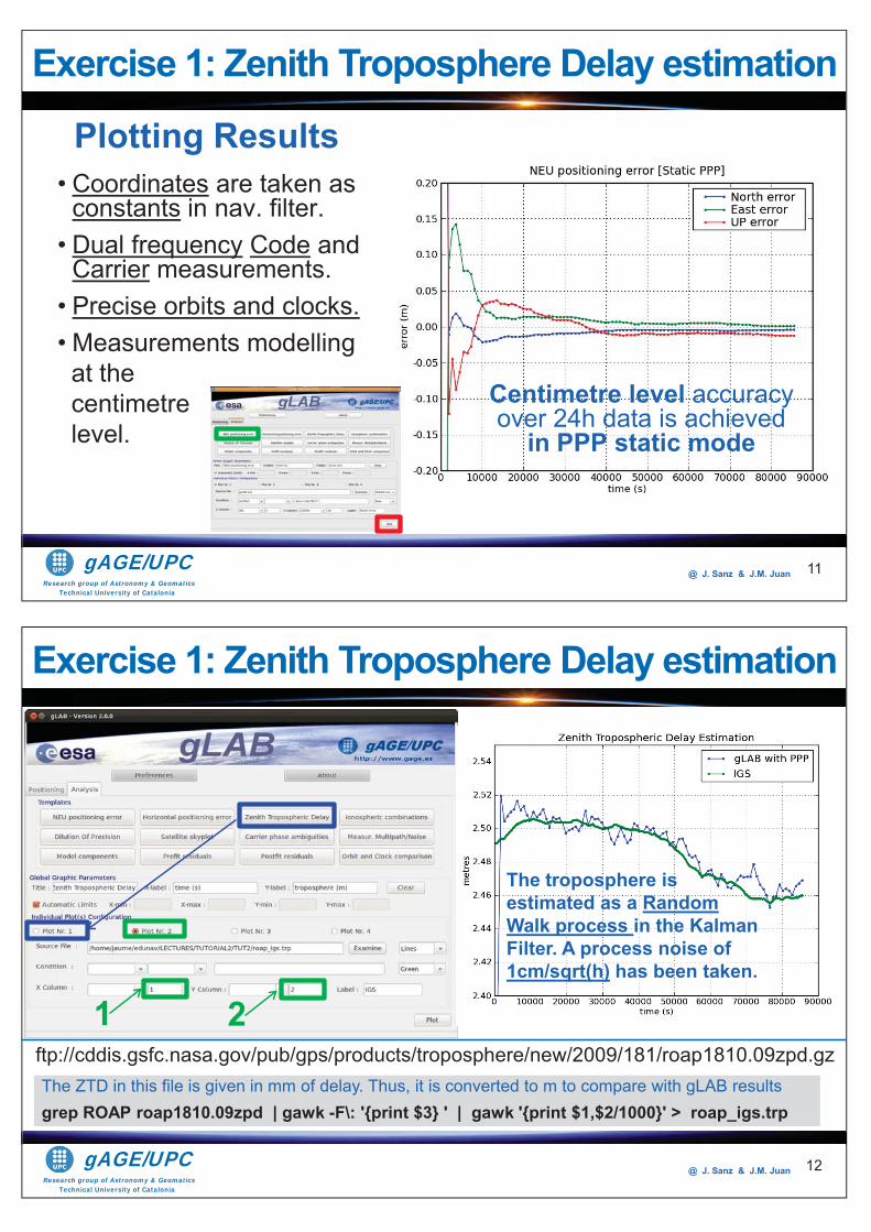
Research group of Astronomy & GeomaticsTechnical University of Catalonia
gAGE/UPC @ J. Sanz & J.M. Juan
Plotting Results• Coordinates are taken as
constants in nav. filter.• Dual frequency Code and
Carrier measurements.• Precise orbits and clocks.• Measurements modellingat the centimetrelevel.
Centimetre level accuracyover 24h data is achieved
in PPP static mode
11
Exercise 1: Zenith Troposphere Delay estimation
Research group of Astronomy & GeomaticsTechnical University of Catalonia
gAGE/UPC @ J. Sanz & J.M. Juan
The ZTD in this file is given in mm of delay. Thus, it is converted to m to compare with gLAB resultsgrep ROAP roap1810.09zpd | gawk -F\: '{print $3} ' | gawk '{print $1,$2/1000}' > roap_igs.trp
ftp://cddis.gsfc.nasa.gov/pub/gps/products/troposphere/new/2009/181/roap1810.09zpd.gz
1 2
The troposphere is estimated as a Random Walk process in the Kalman Filter. A process noise of 1cm/sqrt(h) has been taken.
12
Exercise 1: Zenith Troposphere Delay estimation
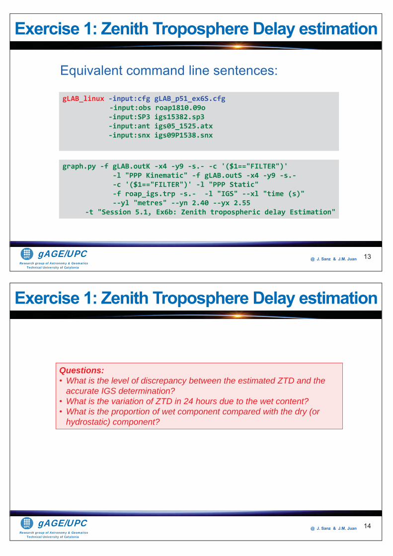
Research group of Astronomy & GeomaticsTechnical University of Catalonia
gAGE/UPC @ J. Sanz & J.M. Juan 13
gLAB_linux -input:cfg gLAB_p51_ex6S.cfg -input:obs roap1810.09o -input:SP3 igs15382.sp3 -input:ant igs05_1525.atx -input:snx igs09P1538.snx
graph.py -f gLAB.outK -x4 -y9 -s.- -c '($1=="FILTER")' -l "PPP Kinematic" -f gLAB.outS -x4 -y9 -s.- -c '($1=="FILTER")' -l "PPP Static" -f roap_igs.trp -s.- -l "IGS" --xl "time (s)" --yl "metres" --yn 2.40 --yx 2.55
-t "Session 5.1, Ex6b: Zenith tropospheric delay Estimation"
Exercise 1: Zenith Troposphere Delay estimation
Equivalent command line sentences:
Research group of Astronomy & GeomaticsTechnical University of Catalonia
gAGE/UPC @ J. Sanz & J.M. Juan 14
Questions: • What is the level of discrepancy between the estimated ZTD and the
accurate IGS determination?• What is the variation of ZTD in 24 hours due to the wet content?• What is the proportion of wet component compared with the dry (or
hydrostatic) component?
Exercise 1: Zenith Troposphere Delay estimation
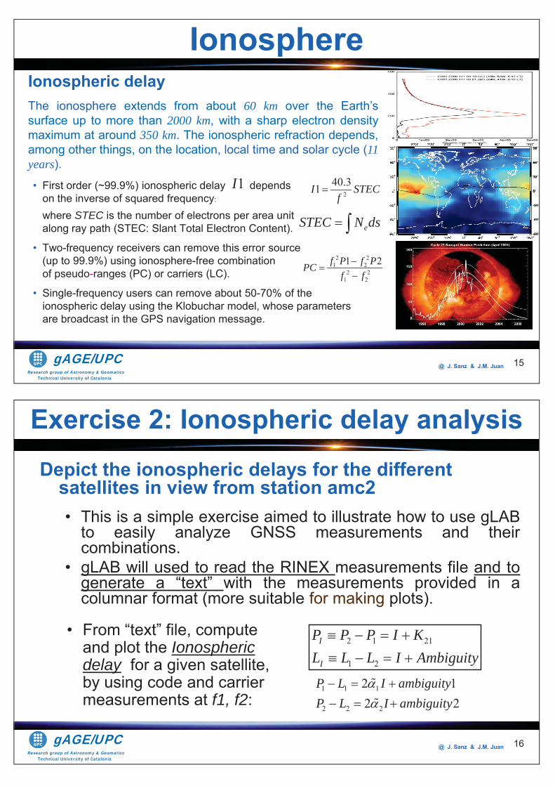
Research group of Astronomy & GeomaticsTechnical University of Catalonia
gAGE/UPC @ J. Sanz & J.M. Juan
• First order (~99.9%) ionospheric delay depends on the inverse of squared frequency:
where STEC is the number of electrons per area unit along ray path (STEC: Slant Total Electron Content).
• Two-frequency receivers can remove this error source (up to 99.9%) using ionosphere-free combination of pseudo-ranges (PC) or carriers (LC).
• Single-frequency users can remove about 50-70% of the ionospheric delay using the Klobuchar model, whose parameters are broadcast in the GPS navigation message.
15
eSTEC N ds
2 21 2
2 21 2
1 2f P f PPCf f
1I
Ionospheric delayThe ionosphere extends from about 60 km over the Earth’ssurface up to more than 2000 km, with a sharp electron densitymaximum at around 350 km. The ionospheric refraction depends,among other things, on the location, local time and solar cycle (11years).
240.31I STECf
Ionosphere
Research group of Astronomy & GeomaticsTechnical University of Catalonia
gAGE/UPC @ J. Sanz & J.M. Juan
Depict the ionospheric delays for the different satellites in view from station amc2 • This is a simple exercise aimed to illustrate how to use gLAB
to easily analyze GNSS measurements and theircombinations.
• gLAB will used to read the RINEX measurements file and togenerate a “text” with the measurements provided in acolumnar format (more suitable for making plots).
Exercise 2: Ionospheric delay analysis
• From “text” file, compute and plot the Ionosphericdelay for a given satellite, by using code and carrier measurements at f1, f2:
2 1 21
1 2
I
I
P P P I KL L L I Ambiguity
1 1 1
2 2 2
2 12 2
P L I ambiguityP L I ambiguity
16
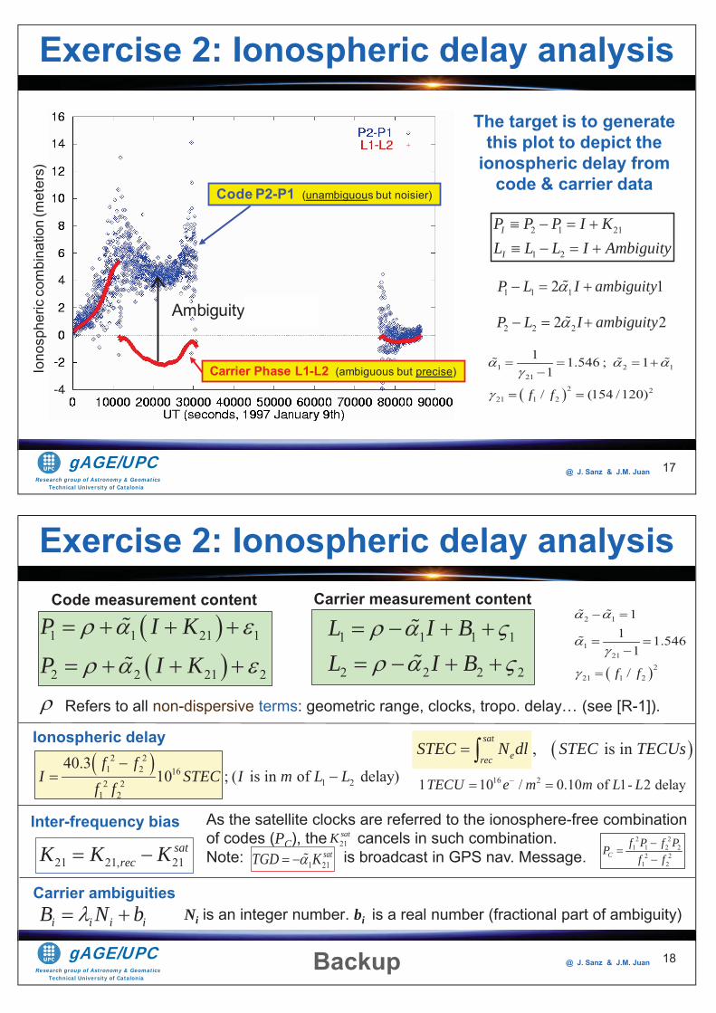
Research group of Astronomy & GeomaticsTechnical University of Catalonia
gAGE/UPC @ J. Sanz & J.M. Juan 17
The target is to generate this plot to depict the
ionospheric delay from code & carrier data
2 1 21
1 2
I
I
P P P I KL L L I Ambiguity
1 1 12 1P L I ambiguity
1 2 121
2 221 1 2
1 1.546 ; 11
/ (154 /120)f f
2 2 22 2P L I ambiguity
Carrier Phase L1-L2 (ambiguous but precise)
Code P2-P1 (unambiguous but noisier)
Ambiguity= P L
Iono
sphe
ric c
ombi
natio
n (m
eter
s)Exercise 2: Ionospheric delay analysis
Research group of Astronomy & GeomaticsTechnical University of Catalonia
gAGE/UPC @ J. Sanz & J.M. Juan 18
1 1 21 1
2 2 21 2
P I K
P I K1 1 1 1
2 2 2 2
L I BL I B
, is in sat
erecSTEC N dl STEC TECUs
16 21 10 / 0.10 of 1- 2 delayTECU e m m L L
2 21 2 16
1 22 21 2
40.310 ; ( is in of delay)
f fI STEC I m L L
f f
21 21, 21sat
recK K K
As the satellite clocks are referred to the ionosphere-free combination of codes (PC), the cancels in such combination. Note: is broadcast in GPS nav. Message.1 21
satTGD K
Refers to all non-dispersive terms: geometric range, clocks, tropo. delay… (see [R-1]).
Ionospheric delay
Inter-frequency bias21satK 2 2
1 1 2 22 2
1 2C
f P f PPf f
i i i iB N bCarrier ambiguities
Ni is an integer number. bi is a real number (fractional part of ambiguity)
2 1
121
221 1 2
11 1.546
1
/f f
Code measurement content Carrier measurement content
Backup
Exercise 2: Ionospheric delay analysis
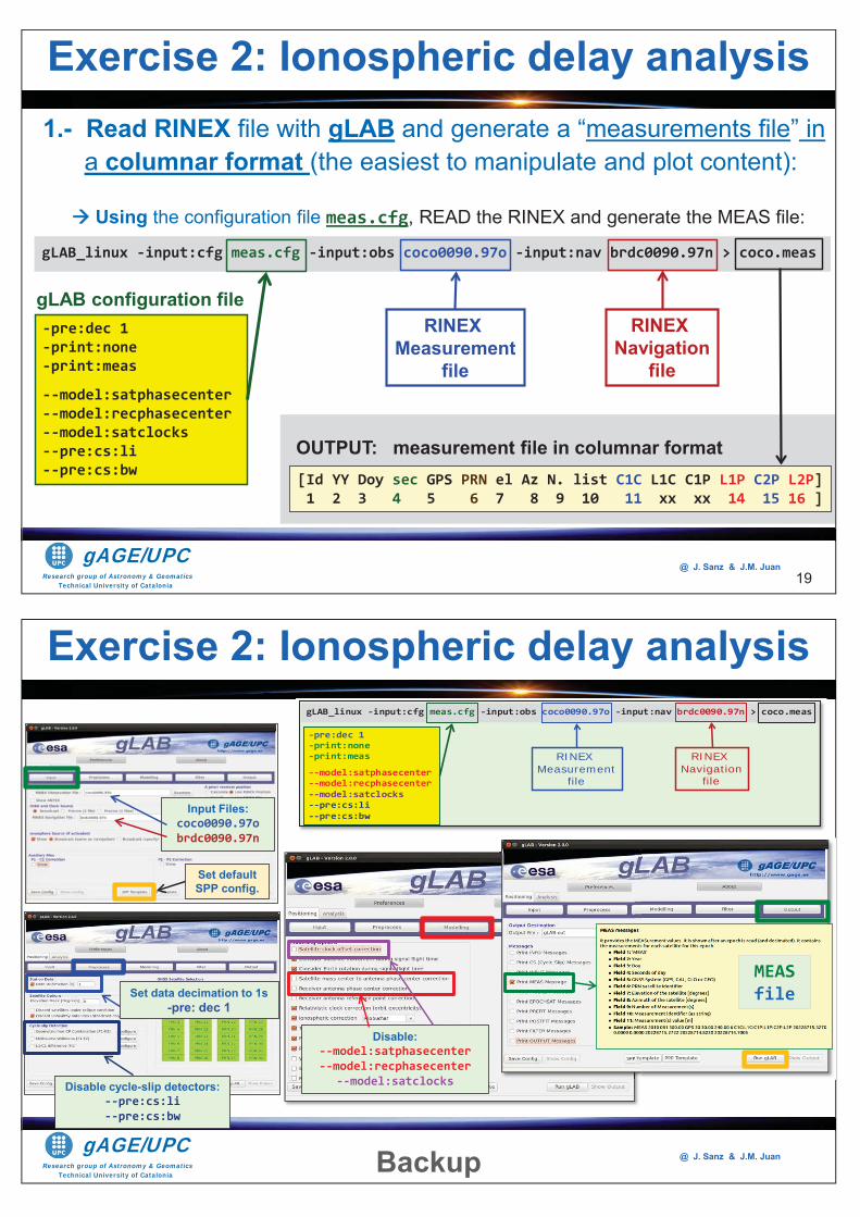
Research group of Astronomy & GeomaticsTechnical University of Catalonia
gAGE/UPC @ J. Sanz & J.M. Juan
1.- Read RINEX file with gLAB and generate a “measurements file” in a columnar format (the easiest to manipulate and plot content):
Using the configuration file meas.cfg, READ the RINEX and generate the MEAS file:
19
[Id YY Doy sec GPS PRN el Az N. list C1C L1C C1P L1P C2P L2P] 1 2 3 4 5 6 7 8 9 10 11 xx xx 14 15 16 ]
gLAB_linux -input:cfg meas.cfg -input:obs coco0090.97o -input:nav brdc0090.97n > coco.meas
-pre:dec 1 -print:none -print:meas
--model:satphasecenter --model:recphasecenter --model:satclocks --pre:cs:li --pre:cs:bw
gLAB configuration fileRINEX
Measurementfile
RINEX Navigation
file
OUTPUT: measurement file in columnar format
Exercise 2: Ionospheric delay analysis
Research group of Astronomy & GeomaticsTechnical University of Catalonia
gAGE/UPC @ J. Sanz & J.M. Juan
gLAB_linux -input:cfg meas.cfg -input:obs coco0090.97o -input:nav brdc0090.97n > coco.meas
-pre:dec 1-print:none-print:meas
--model:satphasecenter--model:recphasecenter--model:satclocks--pre:cs:li--pre:cs:bw
RINEX Measurement
file
RINEX Navigation
file
Disable:--model:satphasecenter --model:recphasecenter
--model:satclocks
Set data decimation to 1s-pre: dec 1
Disable cycle-slip detectors:--pre:cs:li --pre:cs:bw
Input Files:coco0090.97obrdc0090.97n
MEAS file
Set default SPP config.
Backup
Exercise 2: Ionospheric delay analysis
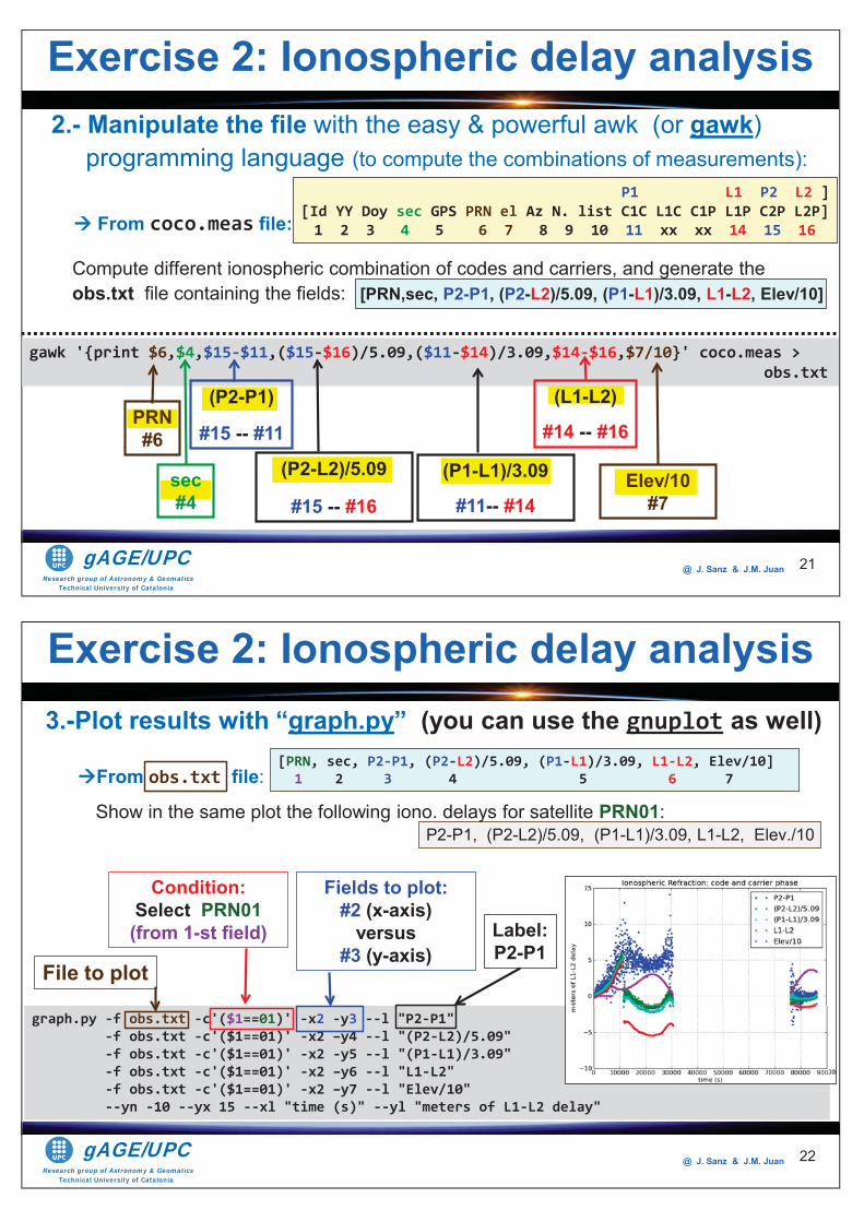
Research group of Astronomy & GeomaticsTechnical University of Catalonia
gAGE/UPC @ J. Sanz & J.M. Juan
2.- Manipulate the file with the easy & powerful awk (or gawk) programming language (to compute the combinations of measurements):
From coco.meas file:
Compute different ionospheric combination of codes and carriers, and generate the obs.txt file containing the fields: [PRN,sec, P2-P1, (P2-L2)/5.09, (P1-L1)/3.09, L1-L2, Elev/10]
21
gawk '{print $6,$4,$15-$11,($15-$16)/5.09,($11-$14)/3.09,$14-$16,$7/10}' coco.meas > obs.txt
PRN#6
sec#4
(P2-P1)
#15 -- #11
(P2-L2)/5.09
#15 -- #16
(P1-L1)/3.09
#11-- #14
(L1-L2)
#14 -- #16
Elev/10#7
P1 L1 P2 L2 ] [Id YY Doy sec GPS PRN el Az N. list C1C L1C C1P L1P C2P L2P] 1 2 3 4 5 6 7 8 9 10 11 xx xx 14 15 16
Exercise 2: Ionospheric delay analysis
Research group of Astronomy & GeomaticsTechnical University of Catalonia
gAGE/UPC @ J. Sanz & J.M. Juan
3.-Plot results with “graph.py” (you can use the gnuplot as well)
From obs.txt file:
Show in the same plot the following iono. delays for satellite PRN01: P2-P1, (P2-L2)/5.09, (P1-L1)/3.09, L1-L2, Elev./10
22
graph.py -f obs.txt -c'($1==01)' -x2 -y3 --l "P2-P1" -f obs.txt -c'($1==01)' -x2 –y4 --l "(P2-L2)/5.09" -f obs.txt -c'($1==01)' -x2 -y5 --l "(P1-L1)/3.09" -f obs.txt -c'($1==01)' -x2 –y6 --l "L1-L2" -f obs.txt -c'($1==01)' -x2 –y7 --l "Elev/10" --yn -10 --yx 15 --xl "time (s)" --yl "meters of L1-L2 delay"
[PRN, sec, P2-P1, (P2-L2)/5.09, (P1-L1)/3.09, L1-L2, Elev/10] 1 2 3 4 5 6 7
File to plot
Condition:Select PRN01
(from 1-st field)
Fields to plot:#2 (x-axis)
versus#3 (y-axis)
Label:P2-P1
Exercise 2: Ionospheric delay analysis
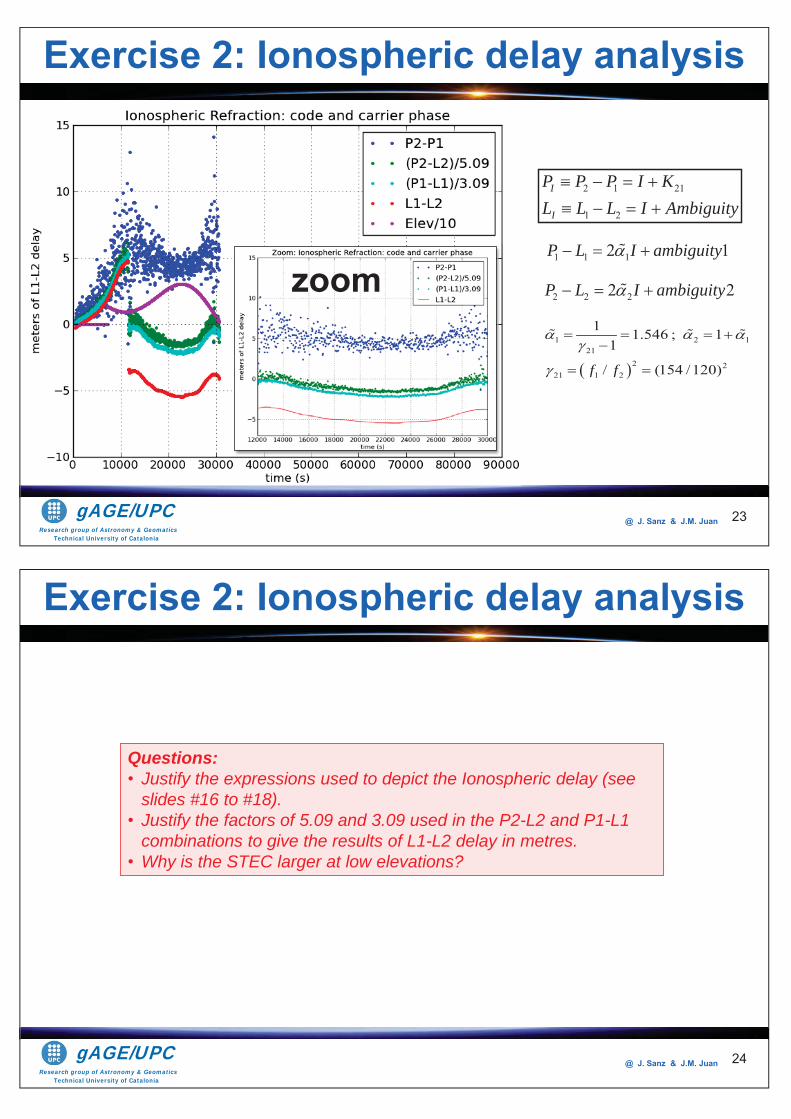
Research group of Astronomy & GeomaticsTechnical University of Catalonia
gAGE/UPC @ J. Sanz & J.M. Juan 23
zoom
2 1 21
1 2
I
I
P P P I KL L L I Ambiguity
1 1 12 1P L I ambiguity
1 2 121
2 221 1 2
1 1.546 ; 11
/ (154 /120)f f
2 2 22 2P L I ambiguity
Exercise 2: Ionospheric delay analysis
Research group of Astronomy & GeomaticsTechnical University of Catalonia
gAGE/UPC @ J. Sanz & J.M. Juan 24
Questions: • Justify the expressions used to depict the Ionospheric delay (see
slides #16 to #18).• Justify the factors of 5.09 and 3.09 used in the P2-L2 and P1-L1
combinations to give the results of L1-L2 delay in metres.• Why is the STEC larger at low elevations?
Exercise 2: Ionospheric delay analysis
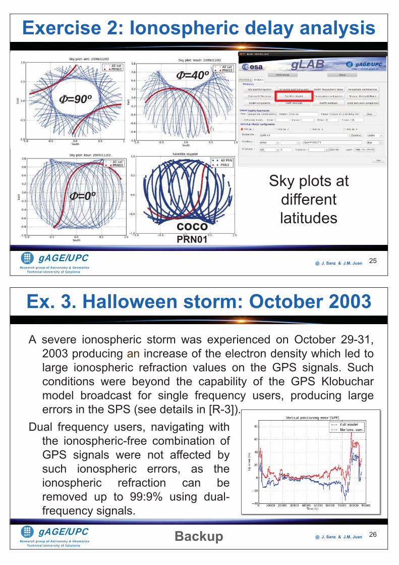
Research group of Astronomy & GeomaticsTechnical University of Catalonia
gAGE/UPC @ J. Sanz & J.M. Juan 25
cocoPRN01
Sky plots at different latitudes
=90º
=40º
=0º
Exercise 2: Ionospheric delay analysis
Research group of Astronomy & GeomaticsTechnical University of Catalonia
gAGE/UPC @ J. Sanz & J.M. Juan
A severe ionospheric storm was experienced on October 29-31,2003 producing an increase of the electron density which led tolarge ionospheric refraction values on the GPS signals. Suchconditions were beyond the capability of the GPS Klobucharmodel broadcast for single frequency users, producing largeerrors in the SPS (see details in [R-3]).
26
Ex. 3. Halloween storm: October 2003
Dual frequency users, navigating withthe ionospheric-free combination ofGPS signals were not affected bysuch ionospheric errors, as theionospheric refraction can beremoved up to 99:9% using dual-frequency signals.
.
Backup
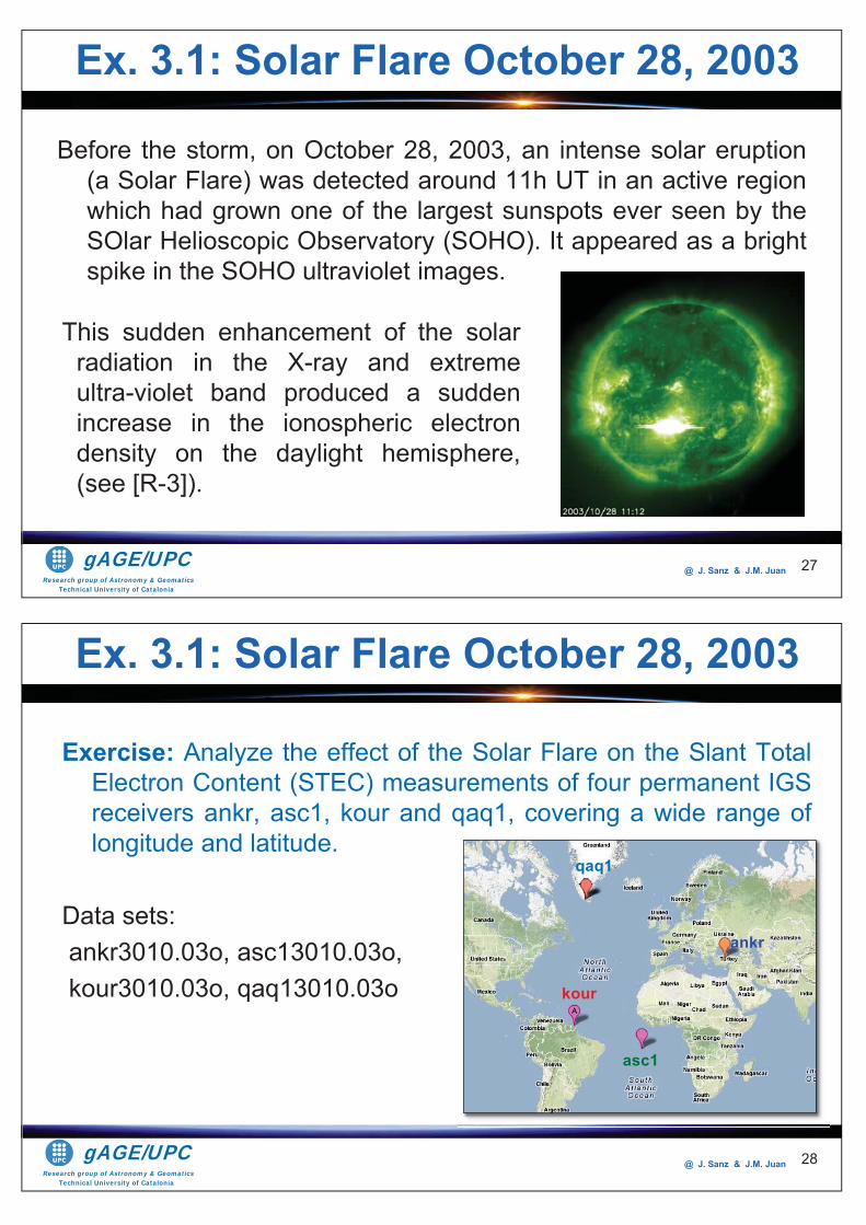
Research group of Astronomy & GeomaticsTechnical University of Catalonia
gAGE/UPC @ J. Sanz & J.M. Juan
Before the storm, on October 28, 2003, an intense solar eruption(a Solar Flare) was detected around 11h UT in an active regionwhich had grown one of the largest sunspots ever seen by theSOlar Helioscopic Observatory (SOHO). It appeared as a brightspike in the SOHO ultraviolet images.
27
This sudden enhancement of the solarradiation in the X-ray and extremeultra-violet band produced a suddenincrease in the ionospheric electrondensity on the daylight hemisphere,(see [R-3]).
Ex. 3.1: Solar Flare October 28, 2003
Research group of Astronomy & GeomaticsTechnical University of Catalonia
gAGE/UPC @ J. Sanz & J.M. Juan
Exercise: Analyze the effect of the Solar Flare on the Slant TotalElectron Content (STEC) measurements of four permanent IGSreceivers ankr, asc1, kour and qaq1, covering a wide range oflongitude and latitude.
Data sets: ankr3010.03o, asc13010.03o,kour3010.03o, qaq13010.03o
28
ankr
qaq1
kour
asc1
Ex. 3.1: Solar Flare October 28, 2003
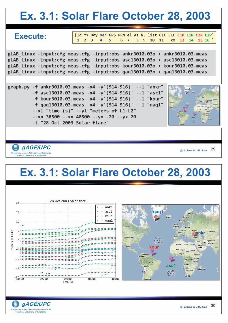
Research group of Astronomy & GeomaticsTechnical University of Catalonia
gAGE/UPC @ J. Sanz & J.M. Juan
Execute:
gLAB_linux -input:cfg meas.cfg -input:obs ankr3010.03o > ankr3010.03.meas gLAB_linux -input:cfg meas.cfg -input:obs asc13010.03o > asc13010.03.meas gLAB_linux -input:cfg meas.cfg -input:obs kour3010.03o > kour3010.03.meas gLAB_linux -input:cfg meas.cfg -input:obs qaq13010.03o > qaq13010.03.meas
graph.py -f ankr3010.03.meas -x4 -y'($14-$16)' --l "ankr" -f asc13010.03.meas -x4 -y'($14-$16)' --l "asc1" -f kour3010.03.meas -x4 -y'($14-$16)' --l "kour" -f qaq13010.03.meas -x4 -y'($14-$16)' --l "qaq1" --xl "time (s)" --yl "meters of L1-L2" --xn 38500 --xx 40500 --yn -20 --yx 20 -t "28 Oct 2003 Solar flare"
ankr
qaq1
kour
asc1
[Id YY Doy sec GPS PRN el Az N. list C1C L1C C1P L1P C2P L2P] 1 2 3 4 5 6 7 8 9 10 11 xx 13 14 15 16 ]
29
Ex. 3.1: Solar Flare October 28, 2003
Research group of Astronomy & GeomaticsTechnical University of Catalonia
gAGE/UPC @ J. Sanz & J.M. Juan 30
ankr
qaq1
kour
asc1
Ex. 3.1: Solar Flare October 28, 2003
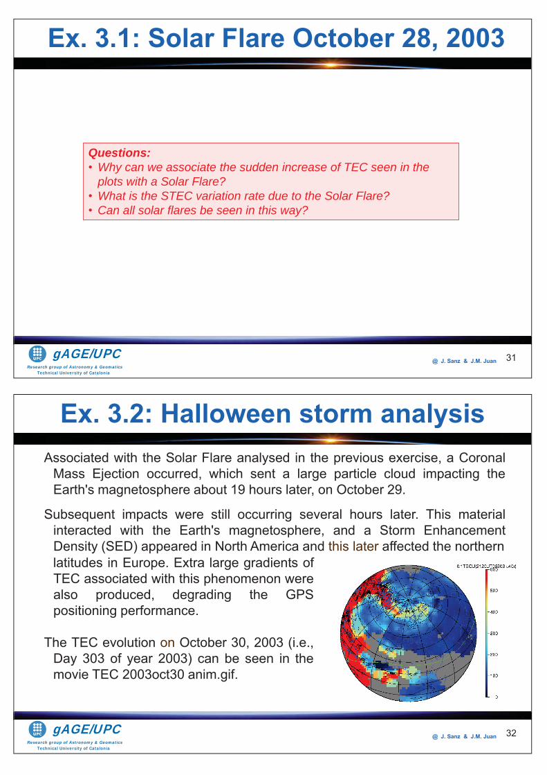
Research group of Astronomy & GeomaticsTechnical University of Catalonia
gAGE/UPC @ J. Sanz & J.M. Juan 31
Questions: • Why can we associate the sudden increase of TEC seen in the
plots with a Solar Flare?• What is the STEC variation rate due to the Solar Flare?• Can all solar flares be seen in this way?
Ex. 3.1: Solar Flare October 28, 2003
Research group of Astronomy & GeomaticsTechnical University of Catalonia
gAGE/UPC @ J. Sanz & J.M. Juan 32
Associated with the Solar Flare analysed in the previous exercise, a CoronalMass Ejection occurred, which sent a large particle cloud impacting theEarth's magnetosphere about 19 hours later, on October 29.
Subsequent impacts were still occurring several hours later. This materialinteracted with the Earth's magnetosphere, and a Storm EnhancementDensity (SED) appeared in North America and this later affected the northernlatitudes in Europe. Extra large gradients ofTEC associated with this phenomenon werealso produced, degrading the GPSpositioning performance.
The TEC evolution on October 30, 2003 (i.e.,Day 303 of year 2003) can be seen in themovie TEC 2003oct30 anim.gif.
Ex. 3.2: Halloween storm analysis
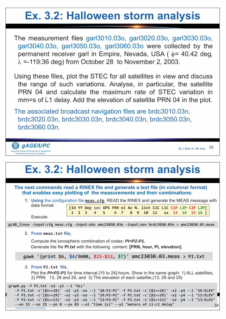
Research group of Astronomy & GeomaticsTechnical University of Catalonia
gAGE/UPC @ J. Sanz & J.M. Juan 33
The measurement files garl3010.03o, garl3020.03o, garl3030.03o,garl3040.03o, garl3050.03o, garl3060.03o were collected by thepermanent receiver garl in Empire, Nevada, USA ( = 40.42 deg
=-119:36 deg) from October 28 to November 2, 2003.
Using these files, plot the STEC for all satellites in view and discussthe range of such variations. Analyse, in particular, the satellitePRN 04 and calculate the maximum rate of STEC variation inmm=s of L1 delay. Add the elevation of satellite PRN 04 in the plot.
The associated broadcast navigation files are brdc3010.03n, brdc3020.03n, brdc3030.03n, brdc3040.03n, brdc3050.03n, brdc3060.03n.
Ex. 3.2: Halloween storm analysis
Research group of Astronomy & GeomaticsTechnical University of Catalonia
gAGE/UPC @ J. Sanz & J.M. Juan
The next commands read a RINEX file and generate a text file (in columnar format) that enables easy plotting of the measurements and their combinations:
1. Using the configuration file meas.cfg, READ the RINEX and generate the MEAS message with data format:
Execute:
2. From meas.txt file, Compute the ionospheric combination of codes: PI=P2-P1.
Generate the file PI.txt with the following content: [PRN, hour, PI, elevation]
3. From PI.txt file,Plot the PI=P2-P1 for time interval [15 to 24].hours. Show in the same graph: 1) ALL satellites, 2) PRN 13, 28 and 29, and 3) The elevation of each satellite.(13, 28 and 29)
34
[Id YY Doy sec GPS PRN el Az N. list C1C L1C C1P L1P C2P L2P] 1 2 3 4 5 6 7 8 9 10 11 xx 13 14 15 16 ]
gawk '{print $6, $4/3600, $15-$13, $7}' amc23030.03.meas > PI.txt
Backup
gLAB_linux -input:cfg meas.cfg -input:obs amc23030.03o -input:nav brdc3030.03n > amc23030.03.meas
graph.py -f PI.txt -x2 -y3 --l "ALL" -f PI.txt -c'($1==28)' -x2 -y3 -so --l "28:P2-P1" -f PI.txt -c'($1==28)' -x2 -y4 --l "29:ELEV" -f PI.txt -c'($1==29)' -x2 -y3 -so --l "29:P2-P1" -f PI.txt -c'($1==29)' -x2 -y4 --l "13:ELEV" -f PI.txt -c'($1==13)' -x2 -y3 -so --l "13:P2-P1" -f PI.txt -c'($1==13)' -x2 -y4 --l "13:ELEV" --xn 15 --xx 25 --yn 0 --yx 85 --xl "time (s)" --yl "meters of L1-L2 delay" 34
Ex. 3.2: Halloween storm analysis
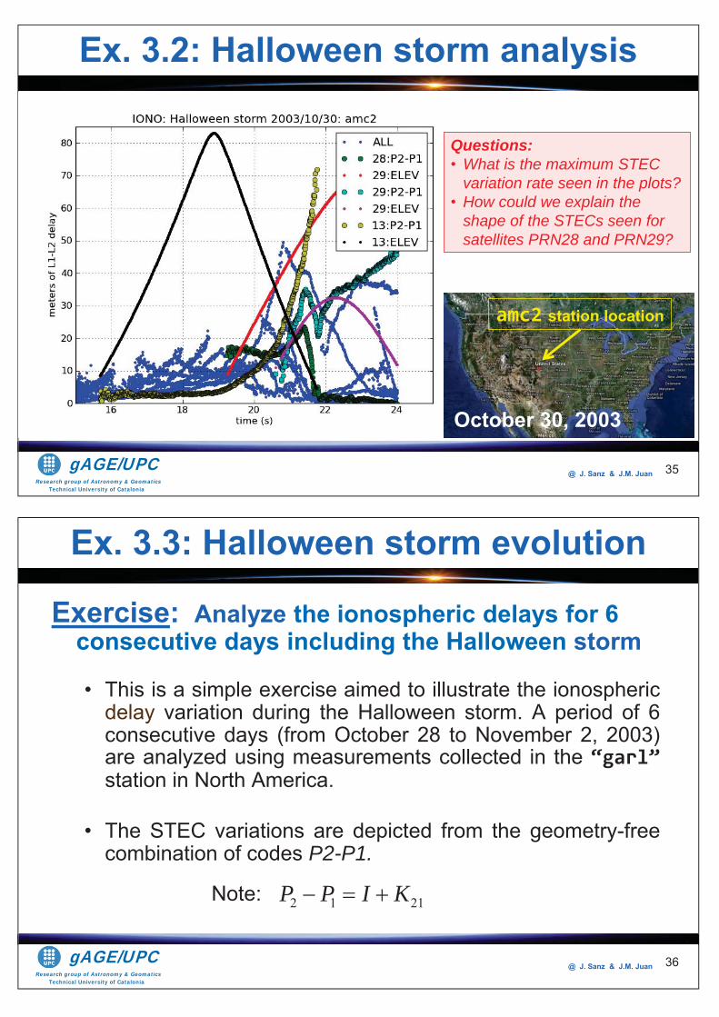
Research group of Astronomy & GeomaticsTechnical University of Catalonia
gAGE/UPC @ J. Sanz & J.M. Juan 35
amc2 station location
October 30, 2003
Ex. 3.2: Halloween storm analysis
Questions: • What is the maximum STEC
variation rate seen in the plots?• How could we explain the
shape of the STECs seen for satellites PRN28 and PRN29?
Research group of Astronomy & GeomaticsTechnical University of Catalonia
gAGE/UPC @ J. Sanz & J.M. Juan
Exercise: Analyze the ionospheric delays for 6 consecutive days including the Halloween storm
• This is a simple exercise aimed to illustrate the ionosphericdelay variation during the Halloween storm. A period of 6consecutive days (from October 28 to November 2, 2003)are analyzed using measurements collected in the “garl” station in North America.
• The STEC variations are depicted from the geometry-freecombination of codes P2-P1.
Note:
36
Ex. 3.3: Halloween storm evolution
2 1 21P P I K
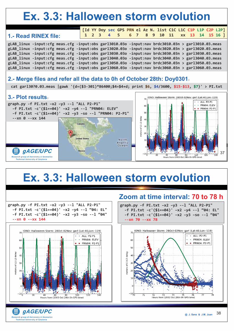
Research group of Astronomy & GeomaticsTechnical University of Catalonia
gAGE/UPC @ J. Sanz & J.M. Juan
gLAB_linux -input:cfg meas.cfg -input:obs garl3010.03o -input:nav brdc3010.03n > garl3010.03.meas gLAB_linux -input:cfg meas.cfg -input:obs garl3020.03o -input:nav brdc3020.03n > garl3020.03.meas gLAB_linux -input:cfg meas.cfg -input:obs garl3030.03o -input:nav brdc3030.03n > garl3030.03.meas gLAB_linux -input:cfg meas.cfg -input:obs garl3040.03o -input:nav brdc3040.03n > garl3040.03.meas gLAB_linux -input:cfg meas.cfg -input:obs garl3050.03o -input:nav brdc3050.03n > garl3050.03.meas gLAB_linux -input:cfg meas.cfg -input:obs garl3060.03o -input:nav brdc3060.03n > garl3060.03.meas
graph.py -f PI.txt –x2 –y3 --l "ALL P2-P1" -f PI.txt -c'($1==04)' –x2 –y4 --l "PRN04: ELEV" -f PI.txt -c'($1==04)' –x2 –y3 –so --l "PRN04: P2-P1" --xn 0 --xx 144
@@@@@@@@@@@@@@@@@@@@@@@@@@@@@@@@@@@@@@@@@@@@@@@@@@@@@@@@@@@@@@@@@@@@@@@@@@@@@@@@@@@@@@ JJJJ. SanSanSannSannnnnnnnnnnzzzzzzzzzzzzzzzzzzzzz &&&& JJJJ.MMMMMMMMMMMMMMMM....... JuaJJJJJJJJJJJJJJJJJuaJJJJJJJJJJJuauaauJ aaannnnnnnnn
cat garl30?0.03.meas |gawk '{d=($3-301)*86400;$4=$4+d; print $6, $4/3600, $15-$13, $7}' > PI.txt
2.- Merge files and refer all the data to 0h of October 28th: Doy0301:
3.- Plot results:
1.- Read RINEX file: [Id YY Doy sec GPS PRN el Az N. list C1C L1C C1P L1P C2P L2P] 1 2 3 4 5 6 7 8 9 10 11 xx 13 14 15 16 ]
Ex. 3.3: Halloween storm evolution
37
Research group of Astronomy & GeomaticsTechnical University of Catalonia
gAGE/UPC @ J. Sanz & J.M. Juan
Zoom at time interval: 70 to 78 h graph.py -f PI.txt –x2 –y3 --l "ALL P2-P1" -f PI.txt -c'($1==04)' –x2 –y4 --l “04: EL" -f PI.txt -c'($1==04)' –x2 –y3 –so --l “04" --xn 0 --xx 144
graph.py -f PI.txt –x2 –y3 --l "ALL P2-P1" -f PI.txt -c'($1==04)' –x2 –y4 --l “04: EL" -f PI.txt -c'($1==04)' –x2 –y3 –so --l “04" --xn 70 --xx 78
Ex. 3.3: Halloween storm evolution
38
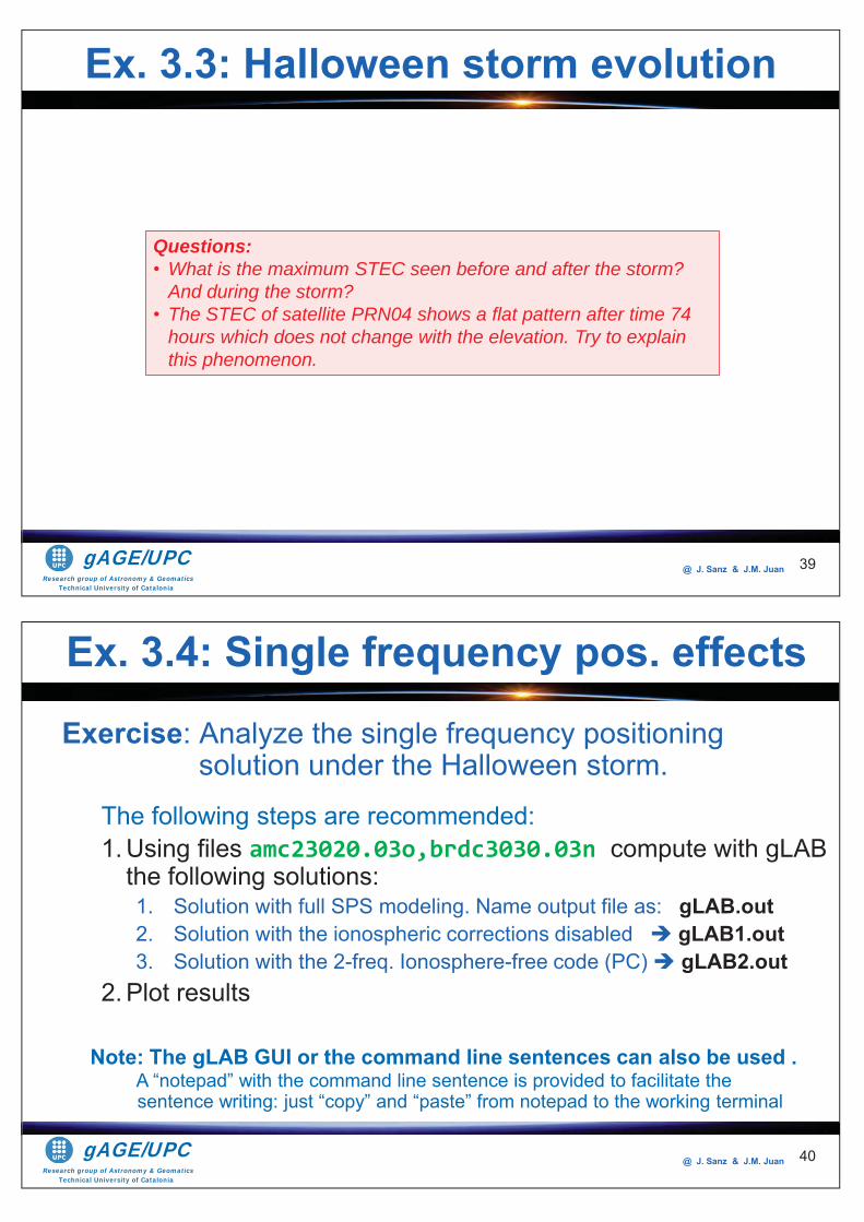
Research group of Astronomy & GeomaticsTechnical University of Catalonia
gAGE/UPC @ J. Sanz & J.M. Juan 39
Questions: • What is the maximum STEC seen before and after the storm?
And during the storm? • The STEC of satellite PRN04 shows a flat pattern after time 74
hours which does not change with the elevation. Try to explain this phenomenon.
Ex. 3.3: Halloween storm evolution
Research group of Astronomy & GeomaticsTechnical University of Catalonia
gAGE/UPC @ J. Sanz & J.M. Juan
Exercise: Analyze the single frequency positioning solution under the Halloween storm.
The following steps are recommended:1. Using files amc23020.03o,brdc3030.03n compute with gLAB
the following solutions:1. Solution with full SPS modeling. Name output file as: gLAB.out2. Solution with the ionospheric corrections disabled gLAB1.out3. Solution with the 2-freq. Ionosphere-free code (PC) gLAB2.out
2. Plot results
40
Ex. 3.4: Single frequency pos. effects
Note: The gLAB GUI or the command line sentences can also be used . A “notepad” with the command line sentence is provided to facilitate the sentence writing: just “copy” and “paste” from notepad to the working terminal
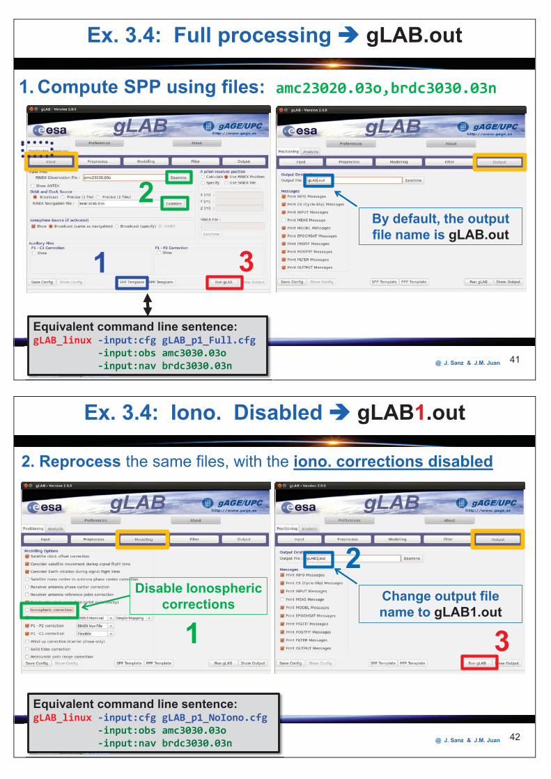
Research group of Astronomy & GeomaticsTechnical University of Catalonia
gAGE/UPC @ J. Sanz & J.M. Juan 41
1. Compute SPP using files: amc23020.03o,brdc3030.03n
1
2
3
TechnTechnicalical UniveUnive yyrsityrsity ofof CatalCataloniaoniaRR
TechnTechnicalicalTechnTechnicalical UniveUniversityrsityUniveUniversityrsity ofofofof CatalCataloniaoniaCatalCataloniaonia
Equivalent command line sentence:gLAB_linux -input:cfg gLAB_p1_Full.cfg -input:obs amc3030.03o -input:nav brdc3030.03n
By default, the output file name is gLAB.out
Ex. 3.4: Full processing gLAB.out
Research group of Astronomy & GeomaticsTechnical University of Catalonia
gAGE/UPC @ J. Sanz & J.M. Juan 42
Ex. 3.4: Iono. Disabled gLAB1.out
Change output file name to gLAB1.out
Disable Ionospheric corrections
31
2
2. Reprocess the same files, with the iono. corrections disabled
TechnTechnicalical UniveUnive yyrsityrsity ofof CatalCataloniaoniaRR
TechnTechnicalicalTechnTechnicalical UniveUniversityrsityUniveUniversityrsity ofofofof CatalCataloniaoniaCatalCataloniaonia
Equivalent command line sentence:gLAB_linux -input:cfg gLAB_p1_NoIono.cfg -input:obs amc3030.03o -input:nav brdc3030.03n
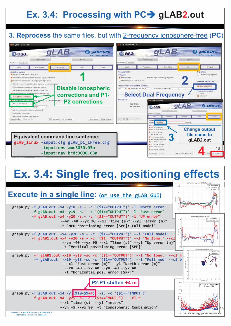
Research group of Astronomy & GeomaticsTechnical University of Catalonia
gAGE/UPC @ J. Sanz & J.M. Juan 43@@@@@@@@@@@@ JJJ... SanSanSanzz & J.M. JuaJuaJJuannn 43
3. Reprocess the same files, but with 2-frequency ionosphere-free (PC)
Ex. 3.4: Processing with PC gLAB2.out
Disable Ionospheric corrections and P1-
P2 corrections
1Select Dual Frequency
2
Change output file name to gLAB2.out 3
4TechnTechnicalical UniveUnive yyrsityrsity ofof CatalCataloniaonia
RRRTechnTechnicalicalTechnical UniveUniversityrsityUniversity ofofof CatalCataloniaoniaCatalonia
Equivalent command line sentence:gLAB_linux -input:cfg gLAB_p1_IFree.cfg -input:obs amc3030.03o -input:nav brdc3030.03n
43
Research group of Astronomy & GeomaticsTechnical University of Catalonia
gAGE/UPC @ J. Sanz & J.M. Juan
graph.py -f gLAB.out -x4 -y18 -s.- -c '($1=="OUTPUT")' -l "North error" -f gLAB.out -x4 -y19 -s.- -c '($1=="OUTPUT")' -l "East error" -f gLAB.out -x4 -y20 -s.- -c '($1=="OUTPUT")' -l "UP error" --yn -40 --yx 70 --xl "time (s)" --yl "error (m)" -t "NEU positioning error [SPP]: Full model"
44
Execute in a single line: (or use the gLAB GUI)
graph.py -f gLAB.out -x4 -y20 -s.- -c '($1=="OUTPUT")' --l "Full model" -f gLAB1.out -x4 -y20 -s.- -c '($1=="OUTPUT")' --l "No Iono." --cl r --yn -40 --yx 90 --xl "Time (s)" --yl "Up error (m)" -t "Vertical positioning error [SPP]"
graph.py -f gLAB1.out -x19 -y18 -so -c '($1=="OUTPUT")' --l "No Iono." --cl r -f gLAB.out -x19 -y18 -so -c '($1=="OUTPUT")' --l "Full mod" --cl b --xl "East error (m)" --yl "North error (m)" --xn -40 --xx 40 --yn -40 --yx 40 -t "Horizontal pos. error [SPP]"
graph.py -f gLAB.out -x4 -y'($10-$9+4)' -s. -c '($1=="INPUT")' -f gLAB.out -x4 -y25 -s. -c '($1=="MODEL")' --cl r --xl "time (s)" --yl "meters" --yn -5 --yx 80 -t "Ionospheric Combination"
@@@@@ JJJJJJJJJJJJJJJJJJJJJJJJJJJJJJJJJ. SSannananSaaaSaaSSaSannSSS nnSSSanSSSanSSSSSanSSSSanSanSSanSSSanSannnSanSannSanSannSanSannSSSaSSanannnSSananSSanSanaaSaSaSSS nnaaaSanSSSSSSSS nSannaaSSSaaaaaaSSSSSSannnnnSanannnaaaaaaaSSSSSSSSSSSSSSSSSSSSSSSSSSSSSSSSSSS zzzzzzzzzzzzzzzzzzzzzzzz &&&&&&&&&&&&&&&&&&&&&&&&&&&&&&&&&&&&&&&&&&&&&&&&&&&&&&&&&&&&&&&&&&&&&&&&&&&&&&&&&&& JJJJJJJJJJJJJJJJJJJJJJJJJJJJJJJJJJJJJJJJJJJJJJJJJJJJJJJJJJJJJJJJJJJJJJJJJJJJ..................MMMMMMMMMMMMMMMMMMMMMMMMMMMMMMMMMMMMMMMMMMMMMMMMMMMMMMMMMMMMMMMMMMMMMMMMMMMMMMMMMMM... JuauJuaJuaJJuaJuaJuJuaJuJuuJJ aJJJJJJJ n 4444444444444444444444444444444444444444444444444444444444444444444444444444444444444444444444444444444
P2-P1 shifted +4 m
r
44
Ex. 3.4: Single freq. positioning effects
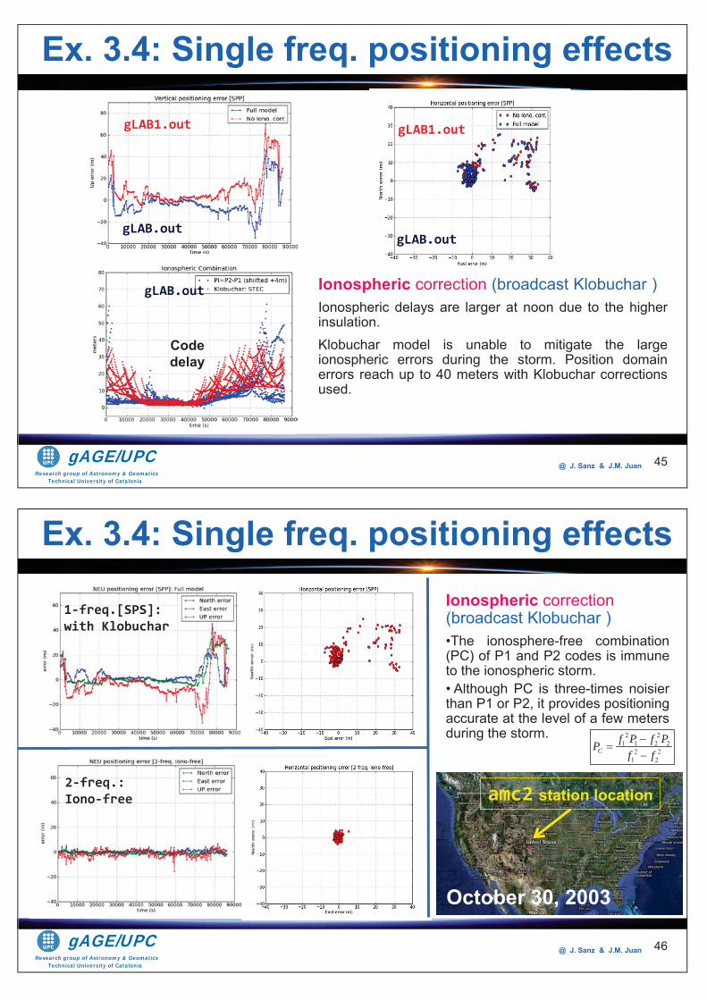
Research group of Astronomy & GeomaticsTechnical University of Catalonia
gAGE/UPC @ J. Sanz & J.M. Juan 45
gLAB.out
gLAB1.out
gLAB.out
Code delay
gLAB.out
gLAB1.out
Ionospheric correction (broadcast Klobuchar )Ionospheric delays are larger at noon due to the higherinsulation.Klobuchar model is unable to mitigate the largeionospheric errors during the storm. Position domainerrors reach up to 40 meters with Klobuchar correctionsused.
Ex. 3.4: Single freq. positioning effects
Research group of Astronomy & GeomaticsTechnical University of Catalonia
gAGE/UPC @ J. Sanz & J.M. Juan 46
2-freq.: Iono-free
1-freq.[SPS]: with Klobuchar
amc2 station location
October 30, 2003
Ionospheric correction(broadcast Klobuchar )•The ionosphere-free combination(PC) of P1 and P2 codes is immuneto the ionospheric storm.• Although PC is three-times noisierthan P1 or P2, it provides positioningaccurate at the level of a few metersduring the storm.
2 21 1 2 2
2 21 2
Cf P f PP
f f
Ex. 3.4: Single freq. positioning effects
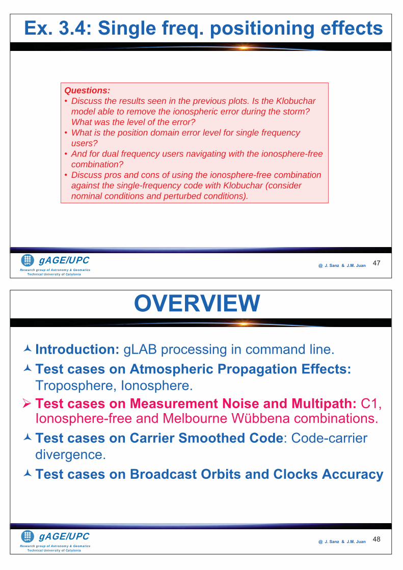
Research group of Astronomy & GeomaticsTechnical University of Catalonia
gAGE/UPC @ J. Sanz & J.M. Juan 47
Questions: • Discuss the results seen in the previous plots. Is the Klobuchar
model able to remove the ionospheric error during the storm? What was the level of the error?
• What is the position domain error level for single frequency users?
• And for dual frequency users navigating with the ionosphere-free combination?
• Discuss pros and cons of using the ionosphere-free combination against the single-frequency code with Klobuchar (consider nominal conditions and perturbed conditions).
Ex. 3.4: Single freq. positioning effects
Research group of Astronomy & GeomaticsTechnical University of Catalonia
gAGE/UPC @ J. Sanz & J.M. Juan
Introduction: gLAB processing in command line.Test cases on Atmospheric Propagation Effects:Troposphere, Ionosphere. Test cases on Measurement Noise and Multipath: C1, Ionosphere-free and Melbourne Wübbena combinations.Test cases on Carrier Smoothed Code: Code-carrier divergence.Test cases on Broadcast Orbits and Clocks Accuracy
OVERVIEW
48
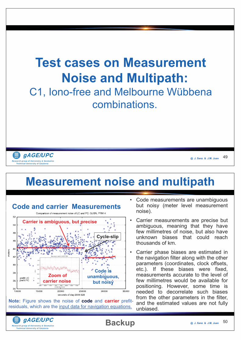
Research group of Astronomy & GeomaticsTechnical University of Catalonia
gAGE/UPC @ J. Sanz & J.M. Juan 49
Test cases on Measurement Noise and Multipath:
C1, Iono-free and Melbourne Wübbena combinations.
Research group of Astronomy & GeomaticsTechnical University of Catalonia
gAGE/UPC @ J. Sanz & J.M. Juan 50
• Code measurements are unambiguousbut noisy (meter level measurementnoise).
• Carrier measurements are precise butambiguous, meaning that they havefew millimetres of noise, but also haveunknown biases that could reachthousands of km.
• Carrier phase biases are estimated inthe navigation filter along with the otherparameters (coordinates, clock offsets,etc.). If these biases were fixed,measurements accurate to the level offew millimetres would be available forpositioning. However, some time isneeded to decorrelate such biasesfrom the other parameters in the filter,and the estimated values are not fullyunbiased.
Code and carrier Measurements
Note: Figure shows the noise of code and carrier prefit-residuals, which are the input data for navigation equations.
Cycle-slip
Code is unambiguous,
but noisy
Carrier is ambiguous, but precise
Zoom ofcarrier noise
Backup
Measurement noise and multipath
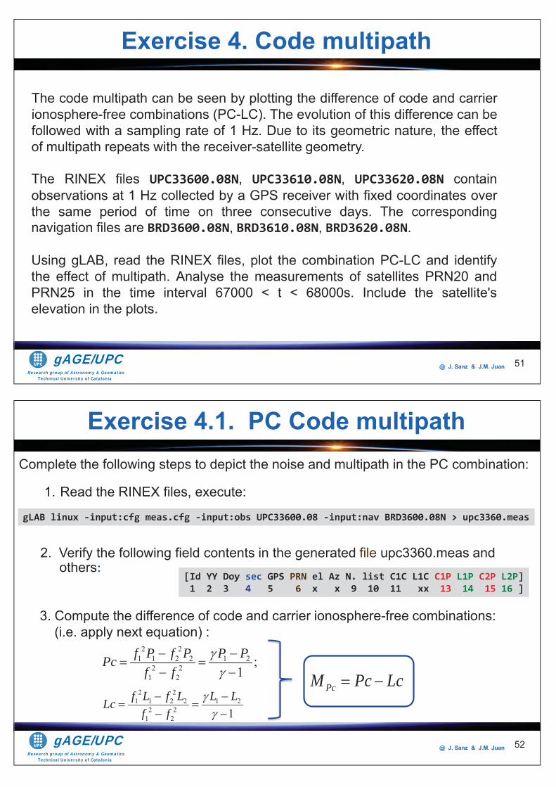
Research group of Astronomy & GeomaticsTechnical University of Catalonia
gAGE/UPC @ J. Sanz & J.M. Juan 51
The code multipath can be seen by plotting the difference of code and carrierionosphere-free combinations (PC-LC). The evolution of this difference can befollowed with a sampling rate of 1 Hz. Due to its geometric nature, the effectof multipath repeats with the receiver-satellite geometry.
The RINEX files UPC33600.08N, UPC33610.08N, UPC33620.08N containobservations at 1 Hz collected by a GPS receiver with fixed coordinates overthe same period of time on three consecutive days. The correspondingnavigation files are BRD3600.08N, BRD3610.08N, BRD3620.08N.
Using gLAB, read the RINEX files, plot the combination PC-LC and identifythe effect of multipath. Analyse the measurements of satellites PRN20 andPRN25 in the time interval 67000 < t < 68000s. Include the satellite'selevation in the plots.
Exercise 4. Code multipath
Research group of Astronomy & GeomaticsTechnical University of Catalonia
gAGE/UPC @ J. Sanz & J.M. Juan
Complete the following steps to depict the noise and multipath in the PC combination:
1. Read the RINEX files, execute:
52
[Id YY Doy sec GPS PRN el Az N. list C1C L1C C1P L1P C2P L2P] 1 2 3 4 5 6 x x 9 10 11 xx 13 14 15 16 ]
gLAB linux -input:cfg meas.cfg -input:obs UPC33600.08 -input:nav BRD3600.08N > upc3360.meas
Exercise 4.1. PC Code multipath
2. Verify the following field contents in the generated file upc3360.meas and others:
3. Compute the difference of code and carrier ionosphere-free combinations: (i.e. apply next equation) :
PcM Pc Lc2 2
1 1 2 2 1 22 2
1 2 1f L f L L LLc
f f
2 21 1 2 2 1 2
2 21 2
;1
f P f P P PPcf f
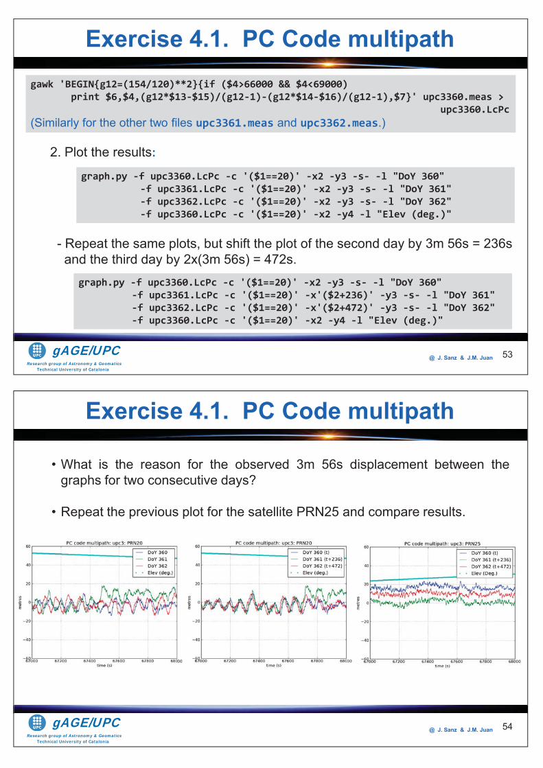
Research group of Astronomy & GeomaticsTechnical University of Catalonia
gAGE/UPC @ J. Sanz & J.M. Juan 53
graph.py -f upc3360.LcPc -c '($1==20)' -x2 -y3 -s- -l "DoY 360" -f upc3361.LcPc -c '($1==20)' -x2 -y3 -s- -l "DoY 361" -f upc3362.LcPc -c '($1==20)' -x2 -y3 -s- -l "DoY 362" -f upc3360.LcPc -c '($1==20)' -x2 -y4 -l "Elev (deg.)"
gawk 'BEGIN{g12=(154/120)**2}{if ($4>66000 && $4<69000) print $6,$4,(g12*$13-$15)/(g12-1)-(g12*$14-$16)/(g12-1),$7}' upc3360.meas > upc3360.LcPc (Similarly for the other two files upc3361.meas and upc3362.meas.)
2. Plot the results:
- Repeat the same plots, but shift the plot of the second day by 3m 56s = 236s and the third day by 2x(3m 56s) = 472s.
graph.py -f upc3360.LcPc -c '($1==20)' -x2 -y3 -s- -l "DoY 360" -f upc3361.LcPc -c '($1==20)' -x'($2+236)' -y3 -s- -l "DoY 361" -f upc3362.LcPc -c '($1==20)' -x'($2+472)' -y3 -s- -l "DoY 362" -f upc3360.LcPc -c '($1==20)' -x2 -y4 -l "Elev (deg.)"
Exercise 4.1. PC Code multipath
Research group of Astronomy & GeomaticsTechnical University of Catalonia
gAGE/UPC @ J. Sanz & J.M. Juan 54
• What is the reason for the observed 3m 56s displacement between thegraphs for two consecutive days?
• Repeat the previous plot for the satellite PRN25 and compare results.
Exercise 4.1. PC Code multipath
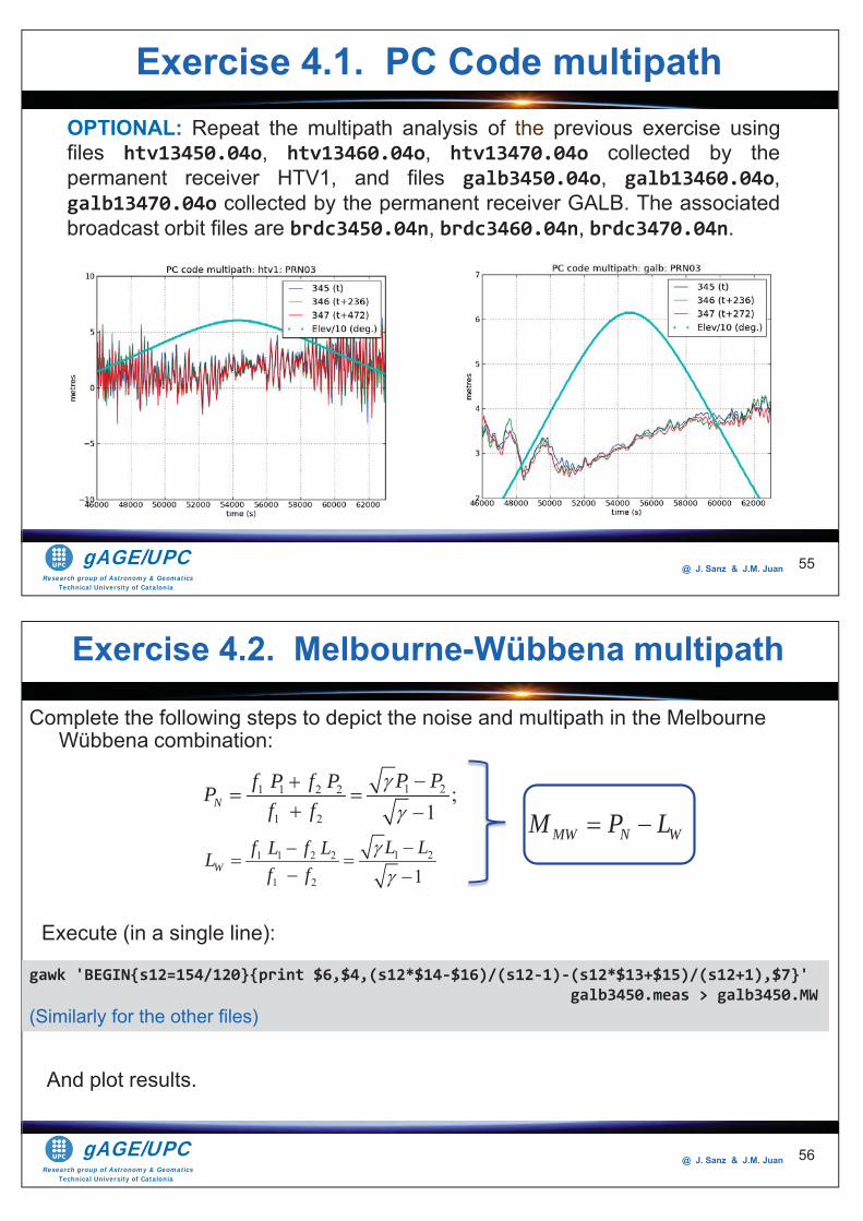
Research group of Astronomy & GeomaticsTechnical University of Catalonia
gAGE/UPC @ J. Sanz & J.M. Juan 55
OPTIONAL: Repeat the multipath analysis of the previous exercise usingfiles htv13450.04o, htv13460.04o, htv13470.04o collected by thepermanent receiver HTV1, and files galb3450.04o, galb13460.04o,galb13470.04o collected by the permanent receiver GALB. The associatedbroadcast orbit files are brdc3450.04n, brdc3460.04n, brdc3470.04n.
Exercise 4.1. PC Code multipath
Research group of Astronomy & GeomaticsTechnical University of Catalonia
gAGE/UPC @ J. Sanz & J.M. Juan
Complete the following steps to depict the noise and multipath in the Melbourne Wübbena combination:
56
Exercise 4.2. Melbourne-Wübbena multipath
Execute (in a single line):
MW N WM P L1 21 1 2 2
1 2 1WL Lf L f LL
f f
1 21 1 2 2
1 2
;1N
P Pf P f PPf f
gawk 'BEGIN{s12=154/120}{print $6,$4,(s12*$14-$16)/(s12-1)-(s12*$13+$15)/(s12+1),$7}' galb3450.meas > galb3450.MW (Similarly for the other files)
And plot results.
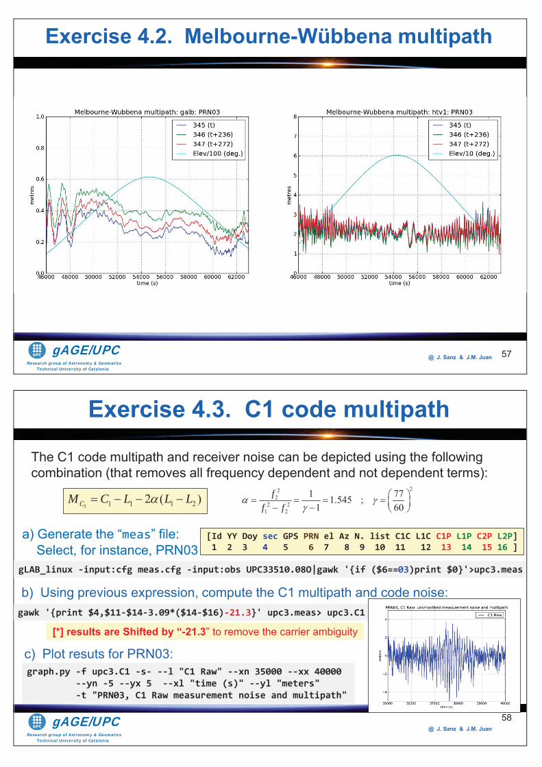
Research group of Astronomy & GeomaticsTechnical University of Catalonia
gAGE/UPC @ J. Sanz & J.M. Juan 57
Exercise 4.2. Melbourne-Wübbena multipath
Research group of Astronomy & GeomaticsTechnical University of Catalonia
gAGE/UPC @ J. Sanz & J.M. Juan
58
The C1 code multipath and receiver noise can be depicted using the following combination (that removes all frequency dependent and not dependent terms):
a) Generate the “meas” file: Select, for instance, PRN03
1 1 1 1 22 ( )CM C L L L
gLAB_linux -input:cfg meas.cfg -input:obs UPC33510.08O|gawk '{if ($6==03)print $0}'>upc3.meas
gawk '{print $4,$11-$14-3.09*($14-$16)-21.3}' upc3.meas> upc3.C1
c) Plot resuts for PRN03:
222
2 21 2
1 771.545 ;1 60
ff f
graph.py -f upc3.C1 -s- --l "C1 Raw" --xn 35000 --xx 40000 --yn -5 --yx 5 --xl "time (s)" --yl "meters" -t "PRN03, C1 Raw measurement noise and multipath"
[*] results are Shifted by “-21.3” to remove the carrier ambiguity
[Id YY Doy sec GPS PRN el Az N. list C1C L1C C1P L1P C2P L2P] 1 2 3 4 5 6 7 8 9 10 11 12 13 14 15 16 ]
b) Using previous expression, compute the C1 multipath and code noise:
Exercise 4.3. C1 code multipath
Research group of Astronomy & GeomaticsTechnical University of Catalonia
gAGE/UPC @ J. Sanz & J.M. Juan
Introduction: gLAB processing in command line.Test cases on Atmospheric Propagation Effects:Troposphere, Ionosphere.Test cases on Measurement Noise and Multipath: C1, Ionosphere-free and Melbourne Wübbena combinations.Test cases on Carrier Smoothed Code: Code-carrier divergence.Test cases on Broadcast Orbits and Clocks Accuracy
OVERVIEW
59
Research group of Astronomy & GeomaticsTechnical University of Catalonia
gAGE/UPC @ J. Sanz & J.M. Juan 60
Test cases on Carrier Smoothed Code:
Code-carrier divergence

Research group of Astronomy & GeomaticsTechnical University of Catalonia
gAGE/UPC @ J. Sanz & J.M. Juan 61
The noisy code P can be smoothed with the precise (but ambiguous) carrier Lmeasurements. This carrier smoothing can be done in real-time applying theHatch filter.
The previous algorithm can be interpreted as real-time alignment of carrier with code:
where
Carrier smoothed code
where [ if ], and [ if ].
1 1ˆ( ) ( ) ( 1) ( ) ( 1)
ˆThe algorithm is initialised with: (1) (1).
n k k N n N k N
nP k P k P k L k L kn n
P P
( )
1 1ˆ( ) ( ) ( 1) ( ) ( 1)
( )k
nP k P k P k L k L kn nL k P L
( ) ( 1)
1 1 1( ) ( ) ( ) ( )k k
nP L P k L k P L P k L kn n n
Carrier Phase L (ambiguous but precise)
Code P (unambiguous but noisier)
Ambiguity= P L
Iono
sphe
ricco
mbi
natio
n(m
eter
s)
Research group of Astronomy & GeomaticsTechnical University of Catalonia
gAGE/UPC @ J. Sanz & J.M. Juan 62
The noisy code can be smoothed with the precise (but ambiguous) carriermeasurements. This carrier smoothing can be done in real-time applying theHatch filter.
The smoothing depends on the time smoothing constant or filter length. The morethe filter length is used, the more smoothed the code is, but (with singlefrequency measurements) a higher code-carrier divergence error is induced bythe ionosphere.
This is because the ionospheric refraction has an opposite sign on code andcarrier, its effect being twice on the difference of code and carrier. This doubleionospheric refraction is propagated forward through the filter, producing a bias.
The error induced by the code-carrier divergence of the ionosphere on thesingle frequency smoothed codes is assessed in this exercise for different filter
lengths.
Carrier smoothed code
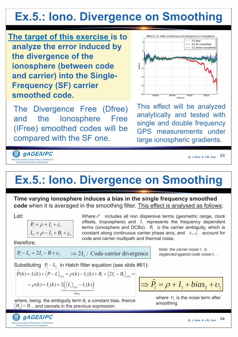
Research group of Astronomy & GeomaticsTechnical University of Catalonia
gAGE/UPC @ J. Sanz & J.M. Juan 63
The target of this exercise is to analyze the error induced by the divergence of the ionosphere (between code and carrier) into the Single-Frequency (SF) carrier smoothed code.
Ex.5.: Iono. Divergence on Smoothing
This effect will be analyzedanalytically and tested withsingle and double frequencyGPS measurements underlarge ionospheric gradients.
The Divergence Free (Dfree)and the Ionosphere Free(IFree) smoothed codes will becompared with the SF one.
Research group of Astronomy & GeomaticsTechnical University of Catalonia
gAGE/UPC @ J. Sanz & J.M. Juan
Where includes all non dispersive terms (geometric range, clockoffsets, troposphere) and represents the frequency dependentterms (ionosphere and DCBs). is the carrier ambiguity, which isconstant along continuous carrier phase arcs, and account forcode and carrier multipath and thermal noise.
64
Time varying ionosphere induces a bias in the single frequency smoothed code when it is averaged in the smoothing filter. This effect is analysed as follows:
Let:
Ex.5.: Iono. Divergence on Smoothing
1 1 1
1 1 1 1
P IL I B
1I1B
1 1,
therefore,
1 1 1 12P L I B 12 : Code-carrier divergenceI
Substituting in Hatch filter equation (see slide #61):1 1P L
1 1 1ˆ
IP I bias
where, being the ambiguity term a constant bias, thence , and cancels in the previous expression
1B1 1B B
1 1 1 1( ) ( )
1 1 1( )
ˆ ( ) ( ) ( ) ( ) 2
( ) ( ) 2 ( )
I
k k
k
bias
P k L k P L k I k B I B
k I k I I k
where is the noise term after smoothing
1
Note: the carrier noise is neglected against code noise .1
1
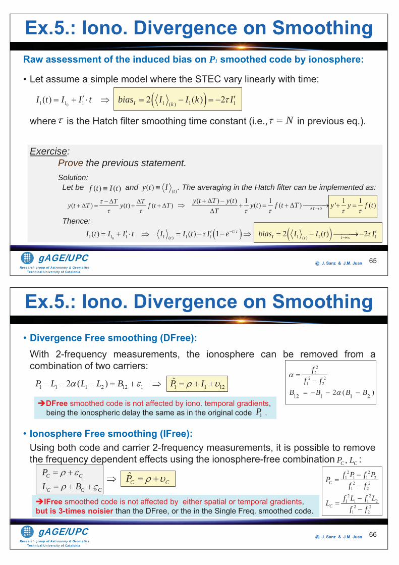
Research group of Astronomy & GeomaticsTechnical University of Catalonia
gAGE/UPC @ J. Sanz & J.M. Juan 65
Raw assessment of the induced bias on P1 smoothed code by ionosphere:
• Let assume a simple model where the STEC vary linearly with time:
where is the Hatch filter smoothing time constant (i.e., in previous eq.).
Exercise: Prove the previous statement.Solution: Let be and . The averaging in the Hatch filter can be implemented as:
Thence:
Ex.5.: Iono. Divergence on Smoothing
01 1 1 1 1 1( )( ) 2 ( ) 2I kI t I I t bias I I k I
N
( ) ( )f t I t ( )( )t
y t I
( ) ( ) ( )T Ty t T y t f t T 0( ) ( ) 1 1 1 1( ) ( ) ' ( )T
y t T y t y t f t T y y f tT
0
/1 1 1 1 1 1 1 1 1( ) ( )( ) ( ) 1 2 ( ) 2t
I tt tI t I I t I I t I e bias I I t I
Research group of Astronomy & GeomaticsTechnical University of Catalonia
gAGE/UPC @ J. Sanz & J.M. Juan 66
• Divergence Free smoothing (DFree):With 2-frequency measurements, the ionosphere can be removed from acombination of two carriers:
Ex.5.: Iono. Divergence on Smoothing
1 1 1 2 12 1 1 1 12ˆ2 ( )P L L L B P I
22
2 21 2
ff f
12 1 1 22 ( )B B B B
• Ionosphere Free smoothing (IFree):Using both code and carrier 2-frequency measurements, it is possible to removethe frequency dependent effects using the ionosphere-free combination :
C C
C C C
PL B
2 21 1 1 2
2 21 2
2 21 1 1 2
2 21 2
C
C
f P f PPf f
f L f LLf f
,C CP L
C CP
DFree smoothed code is not affected by iono. temporal gradients, being the ionospheric delay the same as in the original code .1P
IFree smoothed code is not affected by either spatial or temporal gradients,but is 3-times noisier than the DFree, or the in the Single Freq. smoothed code.
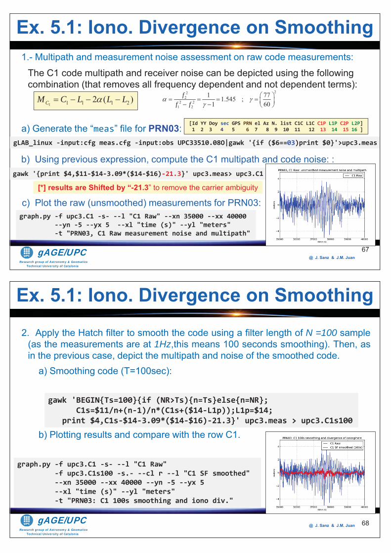
Research group of Astronomy & GeomaticsTechnical University of Catalonia
gAGE/UPC @ J. Sanz & J.M. Juan
67
Ex. 5.1: Iono. Divergence on Smoothing 1.- Multipath and measurement noise assessment on raw code measurements:
The C1 code multipath and receiver noise can be depicted using the following combination (that removes all frequency dependent and not dependent terms):
a) Generate the “meas” file for PRN03:
1 1 1 1 22 ( )CM C L L L
gLAB_linux -input:cfg meas.cfg -input:obs UPC33510.08O|gawk '{if ($6==03)print $0}'>upc3.meas
gawk '{print $4,$11-$14-3.09*($14-$16)-21.3}' upc3.meas> upc3.C1
c) Plot the raw (unsmoothed) measurements for PRN03:
222
2 21 2
1 771.545 ;1 60
ff f
graph.py -f upc3.C1 -s- --l "C1 Raw" --xn 35000 --xx 40000 --yn -5 --yx 5 --xl "time (s)" --yl "meters" -t "PRN03, C1 Raw measurement noise and multipath"
[*] results are Shifted by “-21.3” to remove the carrier ambiguity
[Id YY Doy sec GPS PRN el Az N. list C1C L1C C1P L1P C2P L2P] 1 2 3 4 5 6 7 8 9 10 11 12 13 14 15 16 ]
b) Using previous expression, compute the C1 multipath and code noise: :
Research group of Astronomy & GeomaticsTechnical University of Catalonia
gAGE/UPC @ J. Sanz & J.M. Juan 68
Ex. 5.1: Iono. Divergence on Smoothing
2. Apply the Hatch filter to smooth the code using a filter length of N =100 sample(as the measurements are at 1Hz,this means 100 seconds smoothing). Then, asin the previous case, depict the multipath and noise of the smoothed code.
a) Smoothing code (T=100sec):
b) Plotting results and compare with the row C1.
gawk 'BEGIN{Ts=100}{if (NR>Ts){n=Ts}else{n=NR}; C1s=$11/n+(n-1)/n*(C1s+($14-L1p));L1p=$14; print $4,C1s-$14-3.09*($14-$16)-21.3}' upc3.meas > upc3.C1s100
graph.py -f upc3.C1 -s- --l "C1 Raw" -f upc3.C1s100 -s.- --cl r --l "C1 SF smoothed" --xn 35000 --xx 40000 --yn -5 --yx 5 --xl "time (s)" --yl "meters" -t "PRN03: C1 100s smoothing and iono div."
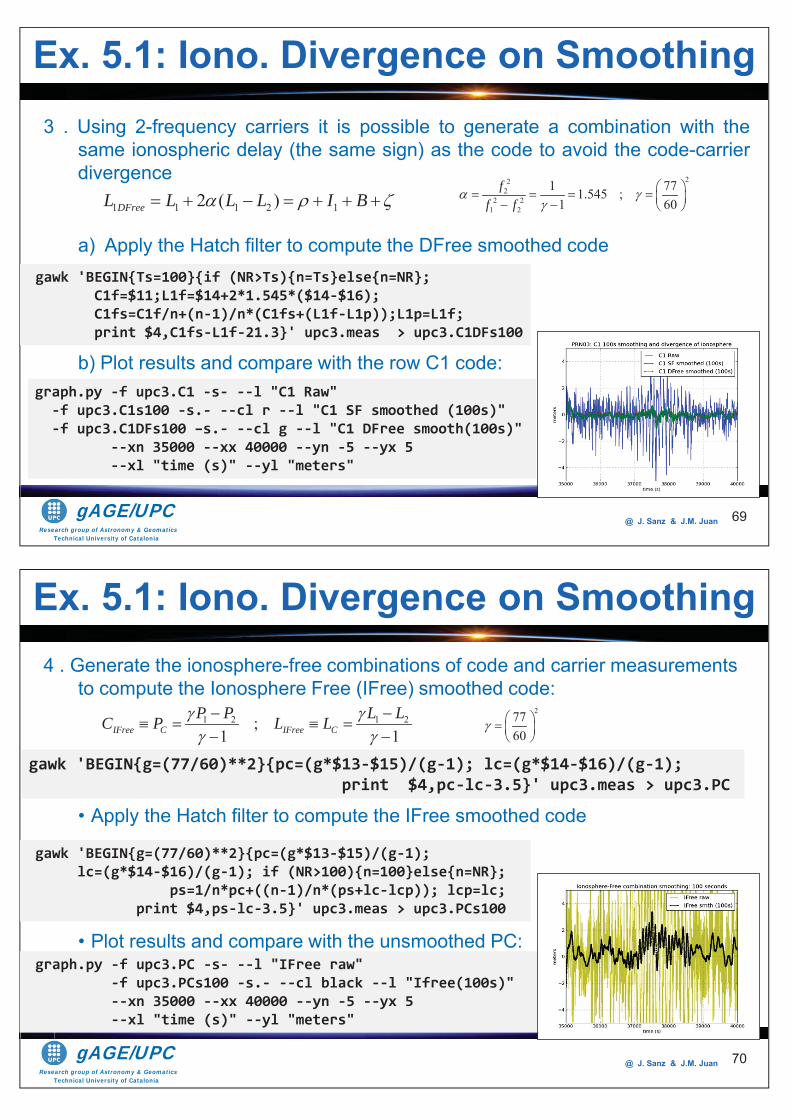
Research group of Astronomy & GeomaticsTechnical University of Catalonia
gAGE/UPC @ J. Sanz & J.M. Juan 69
Ex. 5.1: Iono. Divergence on Smoothing 3 . Using 2-frequency carriers it is possible to generate a combination with the
same ionospheric delay (the same sign) as the code to avoid the code-carrierdivergence
a) Apply the Hatch filter to compute the DFree smoothed code
b) Plot results and compare with the row C1 code:
gawk 'BEGIN{Ts=100}{if (NR>Ts){n=Ts}else{n=NR}; C1f=$11;L1f=$14+2*1.545*($14-$16); C1fs=C1f/n+(n-1)/n*(C1fs+(L1f-L1p));L1p=L1f; print $4,C1fs-L1f-21.3}' upc3.meas > upc3.C1DFs100
1 1 1 2 12 ( )DFreeL L L L I B22
22 2
1 2
1 771.545 ;1 60
ff f
graph.py -f upc3.C1 -s- --l "C1 Raw" -f upc3.C1s100 -s.- --cl r --l "C1 SF smoothed (100s)" -f upc3.C1DFs100 –s.- --cl g --l "C1 DFree smooth(100s)" --xn 35000 --xx 40000 --yn -5 --yx 5 --xl "time (s)" --yl "meters"
Research group of Astronomy & GeomaticsTechnical University of Catalonia
gAGE/UPC @ J. Sanz & J.M. Juan 70
Ex. 5.1: Iono. Divergence on Smoothing 4 . Generate the ionosphere-free combinations of code and carrier measurements
to compute the Ionosphere Free (IFree) smoothed code:
• Apply the Hatch filter to compute the IFree smoothed code
• Plot results and compare with the unsmoothed PC:
gawk 'BEGIN{g=(77/60)**2}{pc=(g*$13-$15)/(g-1); lc=(g*$14-$16)/(g-1); print $4,pc-lc-3.5}' upc3.meas > upc3.PC
27760
1 2 1 2;1 1IFree C IFree C
P P L LC P L L
gawk 'BEGIN{g=(77/60)**2}{pc=(g*$13-$15)/(g-1); lc=(g*$14-$16)/(g-1); if (NR>100){n=100}else{n=NR}; ps=1/n*pc+((n-1)/n*(ps+lc-lcp)); lcp=lc; print $4,ps-lc-3.5}' upc3.meas > upc3.PCs100
graph.py -f upc3.PC -s- --l "IFree raw" -f upc3.PCs100 -s.- --cl black --l "Ifree(100s)" --xn 35000 --xx 40000 --yn -5 --yx 5 --xl "time (s)" --yl "meters"
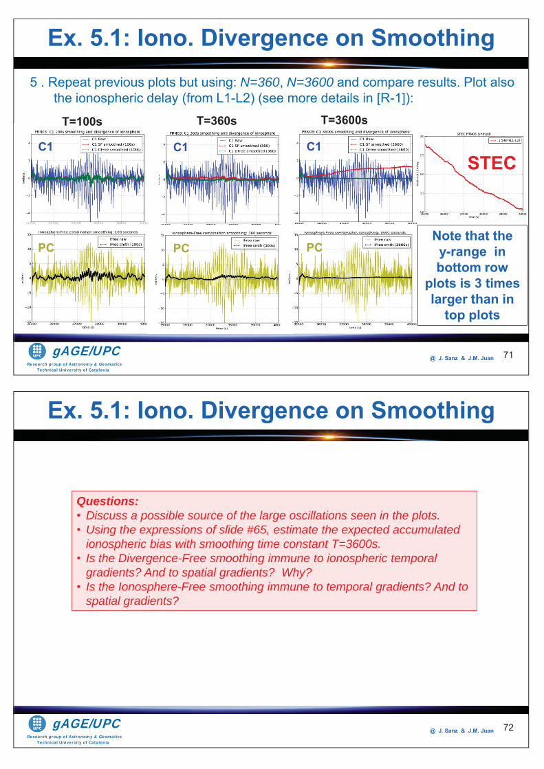
Research group of Astronomy & GeomaticsTechnical University of Catalonia
gAGE/UPC @ J. Sanz & J.M. Juan 71
Ex. 5.1: Iono. Divergence on Smoothing 5 . Repeat previous plots but using: N=360, N=3600 and compare results. Plot also
the ionospheric delay (from L1-L2) (see more details in [R-1]):
STEC
Note that the y-range in bottom row
plots is 3 times larger than in
top plots
T=100s T=360s T=3600s
C1
PC
C1
PC
C1
PC
Research group of Astronomy & GeomaticsTechnical University of Catalonia
gAGE/UPC @ J. Sanz & J.M. Juan 72
Questions: • Discuss a possible source of the large oscillations seen in the plots.• Using the expressions of slide #65, estimate the expected accumulated
ionospheric bias with smoothing time constant T=3600s.• Is the Divergence-Free smoothing immune to ionospheric temporal
gradients? And to spatial gradients? Why?• Is the Ionosphere-Free smoothing immune to temporal gradients? And to
spatial gradients?
Ex. 5.1: Iono. Divergence on Smoothing
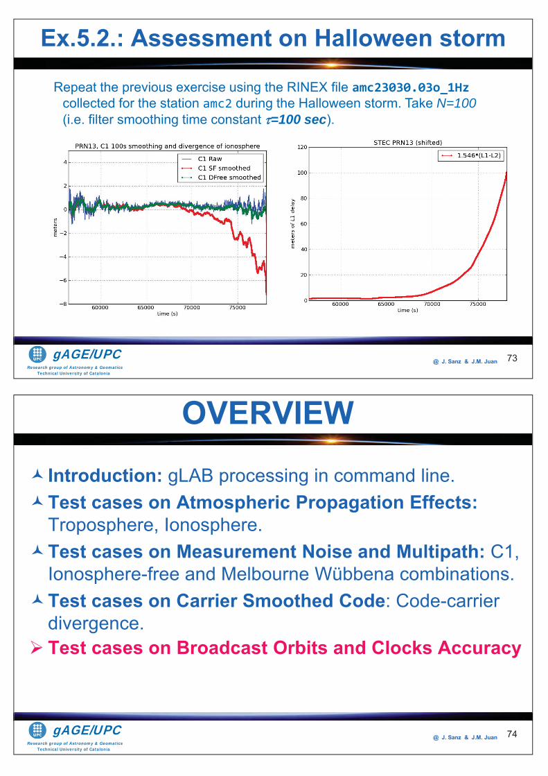
Research group of Astronomy & GeomaticsTechnical University of Catalonia
gAGE/UPC @ J. Sanz & J.M. Juan 73
Repeat the previous exercise using the RINEX file amc23030.03o_1Hz collected for the station amc2 during the Halloween storm. Take N=100(i.e. filter smoothing time constant =100 sec).
Ex.5.2.: Assessment on Halloween storm
Research group of Astronomy & GeomaticsTechnical University of Catalonia
gAGE/UPC @ J. Sanz & J.M. Juan
Introduction: gLAB processing in command line.Test cases on Atmospheric Propagation Effects:Troposphere, Ionosphere.Test cases on Measurement Noise and Multipath: C1, Ionosphere-free and Melbourne Wübbena combinations.Test cases on Carrier Smoothed Code: Code-carrier divergence.Test cases on Broadcast Orbits and Clocks Accuracy
OVERVIEW
74
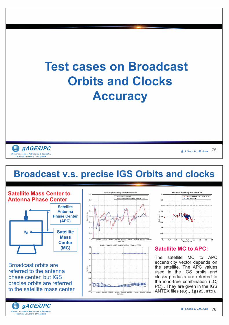
Research group of Astronomy & GeomaticsTechnical University of Catalonia
gAGE/UPC @ J. Sanz & J.M. Juan 75
Test cases on Broadcast Orbits and Clocks
Accuracy
Research group of Astronomy & GeomaticsTechnical University of Catalonia
gAGE/UPC @ J. Sanz & J.M. Juan
Satellite Mass Center to Antenna Phase Center
76
Satellite Mass
Center(MC)
Broadcast orbits are referred to the antenna phase center, but IGS precise orbits are referred to the satellite mass center.
Satellite MC to APC:The satellite MC to APCeccentricity vector depends onthe satellite. The APC valuesused in the IGS orbits andclocks products are referred tothe iono-free combination (LC,PC) . They are given in the IGSANTEX files (e.g., igs05.atx).
Satellite Antenna
Phase Center (APC)
Broadcast v.s. precise IGS Orbits and clocks
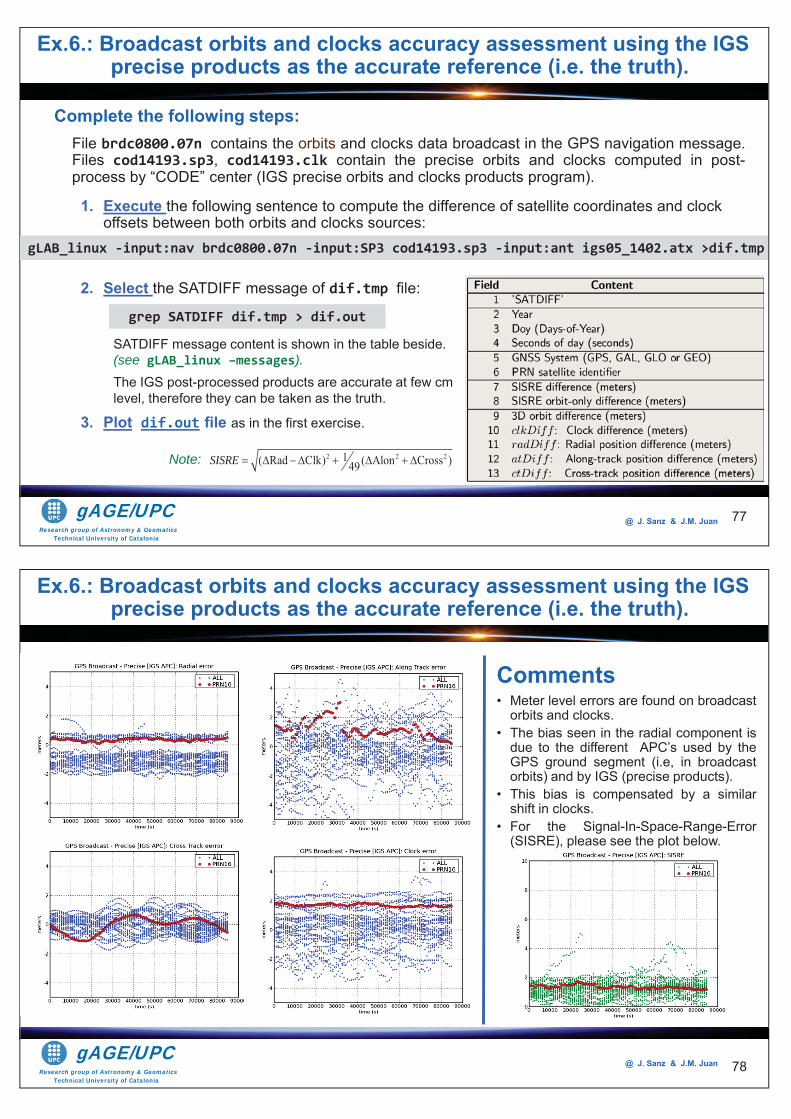
Research group of Astronomy & GeomaticsTechnical University of Catalonia
gAGE/UPC @ J. Sanz & J.M. Juan
Complete the following steps:File brdc0800.07n contains the orbits and clocks data broadcast in the GPS navigation message.Files cod14193.sp3, cod14193.clk contain the precise orbits and clocks computed in post-process by “CODE” center (IGS precise orbits and clocks products program).
1. Execute the following sentence to compute the difference of satellite coordinates and clock offsets between both orbits and clocks sources:
2. Select the SATDIFF message of dif.tmp file:
3. Plot dif.out file as in the first exercise.
Note:
77
gLAB_linux -input:nav brdc0800.07n -input:SP3 cod14193.sp3 -input:ant igs05_1402.atx >dif.tmp
Ex.6.: Broadcast orbits and clocks accuracy assessment using the IGS precise products as the accurate reference (i.e. the truth).
grep SATDIFF dif.tmp > dif.out
SATDIFF message content is shown in the table beside.(see gLAB_linux –messages).The IGS post-processed products are accurate at few cm level, therefore they can be taken as the truth.
2 2 21( Rad Clk) ( Alon Cross )49SISRE
Research group of Astronomy & GeomaticsTechnical University of Catalonia
gAGE/UPC @ J. Sanz & J.M. Juan 78
Comments• Meter level errors are found on broadcast
orbits and clocks.• The bias seen in the radial component is
due to the different APC’s used by theGPS ground segment (i.e, in broadcastorbits) and by IGS (precise products).
• This bias is compensated by a similarshift in clocks.
• For the Signal-In-Space-Range-Error(SISRE), please see the plot below.
Ex.6.: Broadcast orbits and clocks accuracy assessment using the IGS precise products as the accurate reference (i.e. the truth).
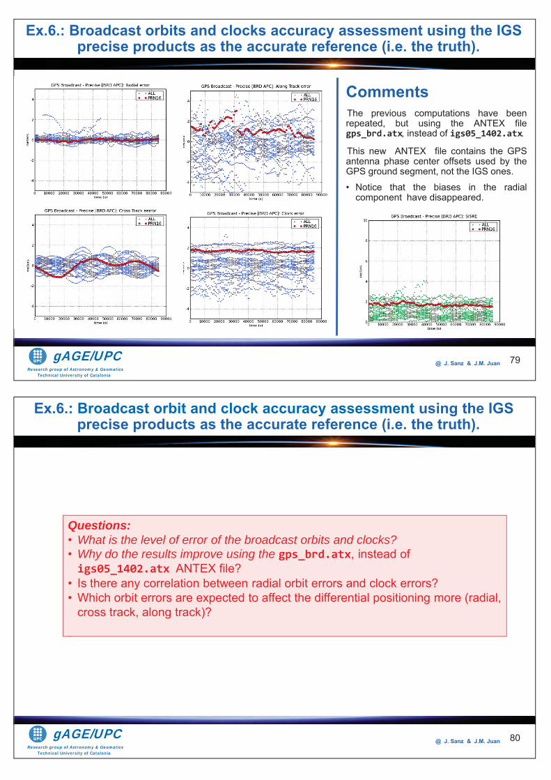
Research group of Astronomy & GeomaticsTechnical University of Catalonia
gAGE/UPC @ J. Sanz & J.M. Juan
CommentsThe previous computations have beenrepeated, but using the ANTEX filegps_brd.atx, instead of igs05_1402.atx.
This new ANTEX file contains the GPSantenna phase center offsets used by theGPS ground segment, not the IGS ones.• Notice that the biases in the radial
component have disappeared.
79
Ex.6.: Broadcast orbits and clocks accuracy assessment using the IGS precise products as the accurate reference (i.e. the truth).
Research group of Astronomy & GeomaticsTechnical University of Catalonia
gAGE/UPC @ J. Sanz & J.M. Juan 80
Questions: • What is the level of error of the broadcast orbits and clocks?• Why do the results improve using the gps_brd.atx, instead of igs05_1402.atx ANTEX file?
• Is there any correlation between radial orbit errors and clock errors?• Which orbit errors are expected to affect the differential positioning more (radial,
cross track, along track)?
Ex.6.: Broadcast orbit and clock accuracy assessment using the IGS precise products as the accurate reference (i.e. the truth).

Research group of Astronomy & GeomaticsTechnical University of Catalonia
gAGE/UPC @ J. Sanz & J.M. Juan 81
Thanks for yourattention
Research group of Astronomy & GeomaticsTechnical University of Catalonia
gAGE/UPC @ J. Sanz & J.M. Juan 82
R-1: J. Sanz-Subirana, J.M. Jaun-Zoroza, M. Hernández-Pajares. GNSS Data processing.Volume-I and Volume-II. ESA Publications Division, 2012.R-2: J. Sanz-Subirana, J.M. Jaun-Zoroza, M. Hernández-Pajares. Tutorial on GNSS DataProcessing Laboratory Exercises. ESAInternational Summer School on GNSS, 2010.R-3: Hernández-Pajares M., J.M. Juan, J. Sanz, "EGNOS Test Bed IonosphericCorrections Under the October and November 2003 Storms", IEEE Transactions onGeoscience and Remote Sensing, Vol.43(10), pp.2283-2293, 2005.
Bibliography
Research group of Astronomy & GeomaticsTechnical University of Catalonia
gAGE/UPC @ J. Sanz & J.M. Juan
The ESA/UPC GNSS-Lab Tool suite (gLAB) has beendeveloped under the ESA Education Office contract N.P1081434.The other data files used in this study were acquired as part ofNASA's Earth Science Data Systems and archived anddistributed by the Crustal Dynamics Data Information System(CDDIS).To Adrià Rovira-Garcia for his contribution to the edition of thismaterial and gLAB updating.
83
Acknowledgements

Research group of Astronomy & GeomaticsTechnical University of Catalonia
gAGE/UPC @ J. Sanz & J.M. Juan 1
Tutorial 3Differential Positioning
with code measurements
Contact: [email protected] site: http://www.gage.upc.edu
Slides associated to gLAB version 2.0.0
Research group of Astronomy & GeomaticsTechnical University of Catalonia
gAGE/UPC @ J. Sanz & J.M. Juan 3
This tutorial is devoted to analysing and assessing the differential positioning with code pseudorange measurements. Four different permanent receivers and two baselines 280km and 51km are considered.
The atmospheric effects on differential positioning are the subject of the first session. The differential tropospheric and ionospheric delays are analysed for the two baselines considered and the absolute and differential user solution are computed and assessed.
The ephemeris error on differential positioning is the subject of the second session. A 2000 metres of Along-Track error is simulated by manipulating the broadcast message, and the impact of this error on range and user domains is assessed for absolute and differential positioning. A theoretical expression to predict the range error on a given baseline is also verified in the last part of this session. Detailed guidelines for self-learning students are provided in this tutorial and in its associated notepad text file.
All software tools (including gLAB) and associated files for the laboratory session are included in the CD-ROM or USB stick associated with this tutorial.
Aim of this tutorial
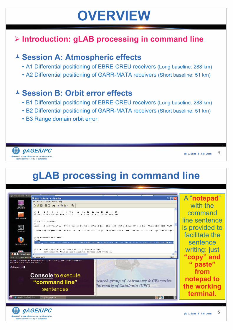
Research group of Astronomy & GeomaticsTechnical University of Catalonia
gAGE/UPC @ J. Sanz & J.M. Juan
Introduction: gLAB processing in command line
Session A: Atmospheric effects• A1 Differential positioning of EBRE-CREU receivers (Long baseline: 288 km) • A2 Differential positioning of GARR-MATA receivers (Short baseline: 51 km)
Session B: Orbit error effects• B1 Differential positioning of EBRE-CREU receivers (Long baseline: 288 km) • B2 Differential positioning of GARR-MATA receivers (Short baseline: 51 km)• B3 Range domain orbit error.
OVERVIEW
4
Research group of Astronomy & GeomaticsTechnical University of Catalonia
gAGE/UPC @ J. Sanz & J.M. Juan 5
Console to execute “command line”
sentences
A “notepad” with the
command line sentence is provided to facilitate the
sentence writing: just “copy” and
“ paste” from
notepad to the working
terminal.
gLAB processing in command line
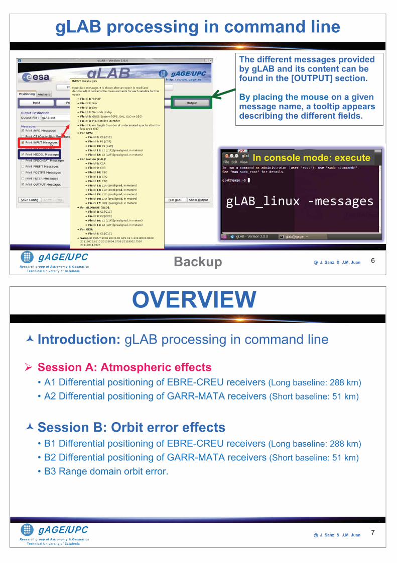
Research group of Astronomy & GeomaticsTechnical University of Catalonia
gAGE/UPC @ J. Sanz & J.M. Juan 6
The different messages provided by gLAB and its content can be found in the [OUTPUT] section.
By placing the mouse on a given message name, a tooltip appears describing the different fields.
Backup
gLAB_linux -messages
In console mode: execute
gLAB processing in command line
Research group of Astronomy & GeomaticsTechnical University of Catalonia
gAGE/UPC @ J. Sanz & J.M. Juan
Introduction: gLAB processing in command line
Session A: Atmospheric effects• A1 Differential positioning of EBRE-CREU receivers (Long baseline: 288 km) • A2 Differential positioning of GARR-MATA receivers (Short baseline: 51 km)
Session B: Orbit error effects• B1 Differential positioning of EBRE-CREU receivers (Long baseline: 288 km) • B2 Differential positioning of GARR-MATA receivers (Short baseline: 51 km)• B3 Range domain orbit error.
OVERVIEW
7
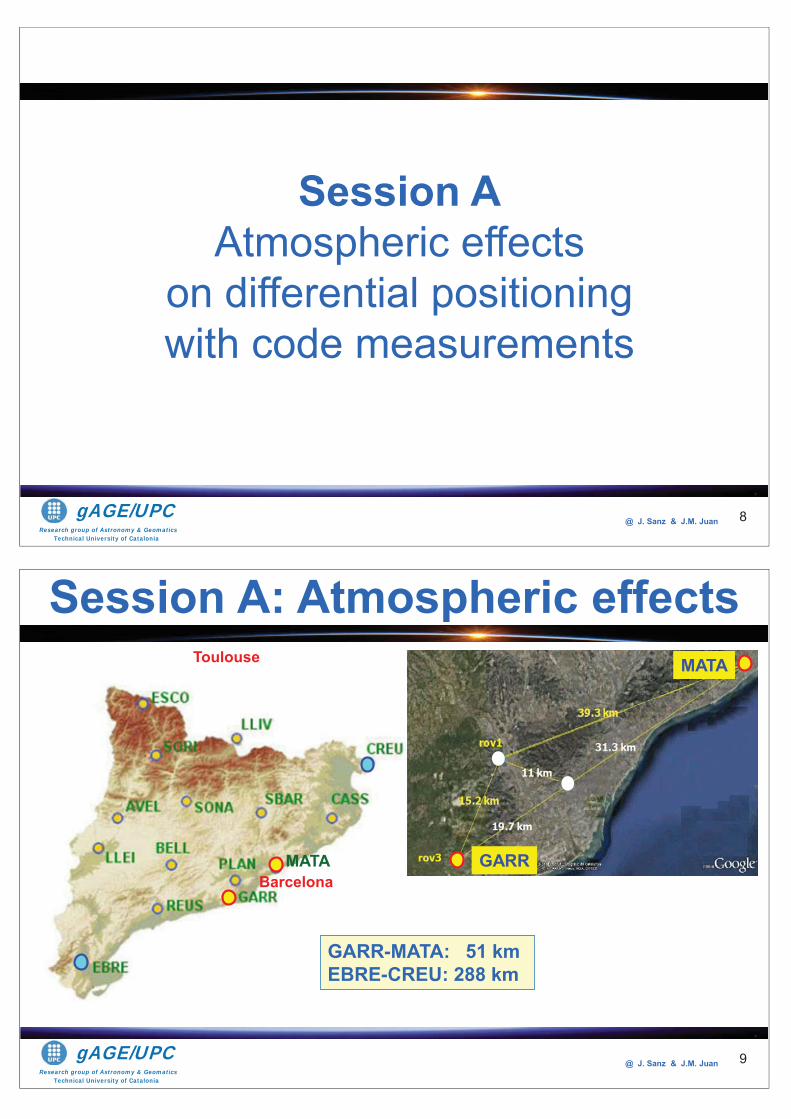
Research group of Astronomy & GeomaticsTechnical University of Catalonia
gAGE/UPC @ J. Sanz & J.M. Juan 8
Session AAtmospheric effects
on differential positioning with code measurements
Research group of Astronomy & GeomaticsTechnical University of Catalonia
gAGE/UPC @ J. Sanz & J.M. Juan 9
MATA
GARR
GARR-MATA: 51 kmEBRE-CREU: 288 km
Barcelona
Toulouse
MATA
Session A: Atmospheric effects
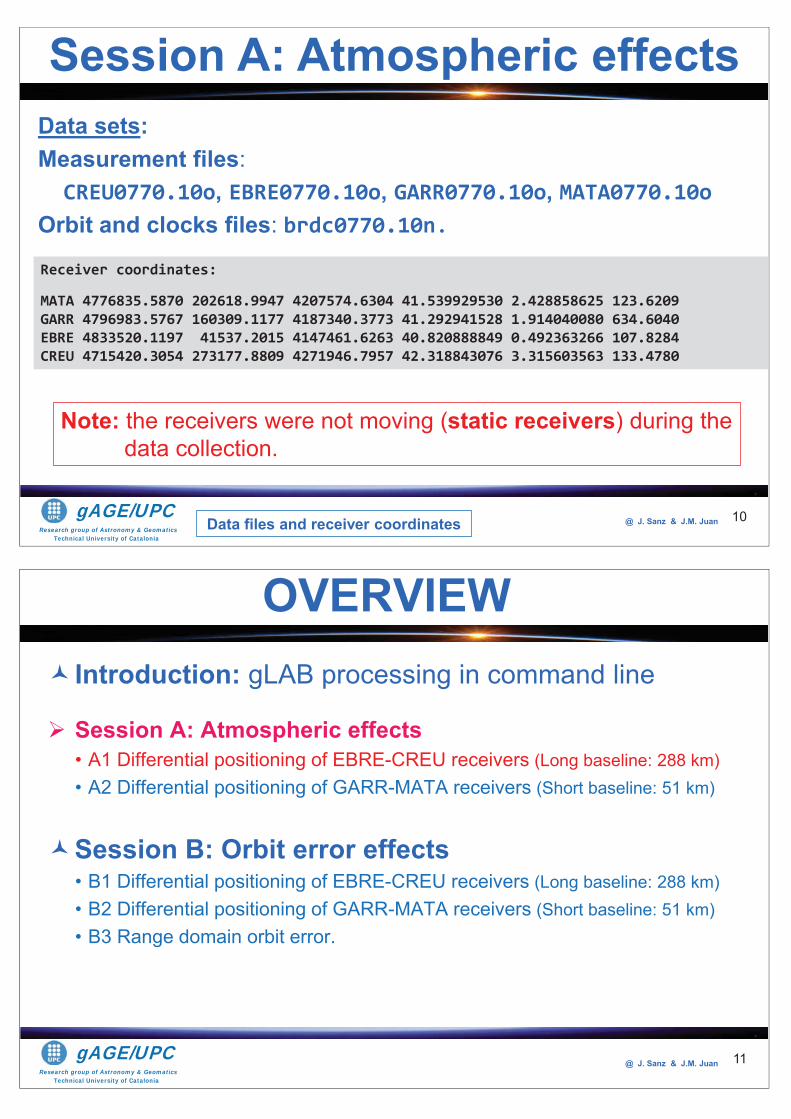
Research group of Astronomy & GeomaticsTechnical University of Catalonia
gAGE/UPC @ J. Sanz & J.M. Juan
Data sets:Measurement files:
CREU0770.10o, EBRE0770.10o, GARR0770.10o, MATA0770.10oOrbit and clocks files: brdc0770.10n.
10
Receiver coordinates:
MATA 4776835.5870 202618.9947 4207574.6304 41.539929530 2.428858625 123.6209GARR 4796983.5767 160309.1177 4187340.3773 41.292941528 1.914040080 634.6040EBRE 4833520.1197 41537.2015 4147461.6263 40.820888849 0.492363266 107.8284CREU 4715420.3054 273177.8809 4271946.7957 42.318843076 3.315603563 133.4780
Data files and receiver coordinates
Session A: Atmospheric effects
Note: the receivers were not moving (static receivers) during the data collection.
Research group of Astronomy & GeomaticsTechnical University of Catalonia
gAGE/UPC @ J. Sanz & J.M. Juan
Introduction: gLAB processing in command line
Session A: Atmospheric effects• A1 Differential positioning of EBRE-CREU receivers (Long baseline: 288 km) • A2 Differential positioning of GARR-MATA receivers (Short baseline: 51 km)
Session B: Orbit error effects• B1 Differential positioning of EBRE-CREU receivers (Long baseline: 288 km) • B2 Differential positioning of GARR-MATA receivers (Short baseline: 51 km)• B3 Range domain orbit error.
OVERVIEW
11
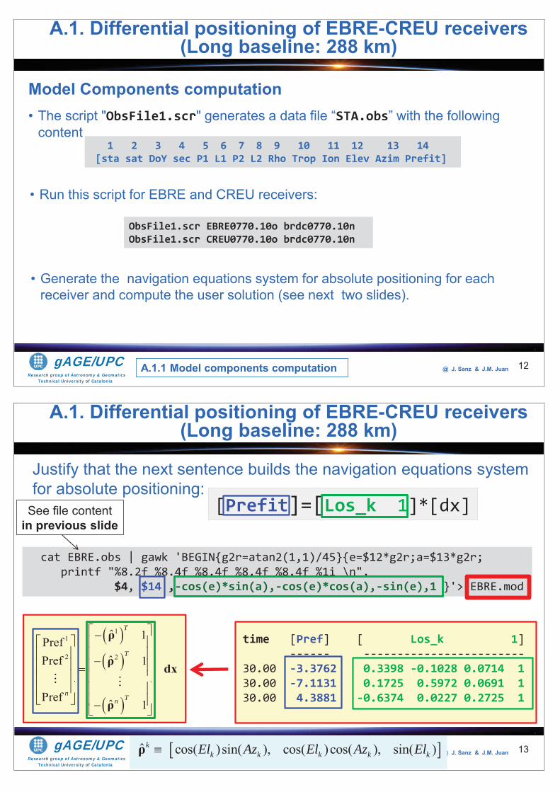
Research group of Astronomy & GeomaticsTechnical University of Catalonia
gAGE/UPC @ J. Sanz & J.M. Juan
Model Components computation• The script "ObsFile1.scr" generates a data file “STA.obs” with the following
content
12
1 2 3 4 5 6 7 8 9 10 11 12 13 14[sta sat DoY sec P1 L1 P2 L2 Rho Trop Ion Elev Azim Prefit]
• Run this script for EBRE and CREU receivers:
ObsFile1.scr EBRE0770.10o brdc0770.10nObsFile1.scr CREU0770.10o brdc0770.10n
• Generate the navigation equations system for absolute positioning for each receiver and compute the user solution (see next two slides).
A.1.1 Model components computation
A.1. Differential positioning of EBRE-CREU receivers (Long baseline: 288 km)
Research group of Astronomy & GeomaticsTechnical University of Catalonia
gAGE/UPC @ J. Sanz & J.M. Juan 13
cat EBRE.obs | gawk 'BEGIN{g2r=atan2(1,1)/45}{e=$12*g2r;a=$13*g2r;printf "%8.2f %8.4f %8.4f %8.4f %8.4f %1i \n",
$4, $14 ,-cos(e)*sin(a),-cos(e)*cos(a),-sin(e),1 }'> EBRE.mod
Justify that the next sentence builds the navigation equations system for absolute positioning:
[Prefit]=[Los_k 1]*[dx]
time [Pref] [ Los_k 1] ------ ------------------------
30.00 -3.3762 0.3398 -0.1028 0.0714 130.00 -7.1131 0.1725 0.5972 0.0691 1 30.00 4.3881 -0.6374 0.0227 0.2725 1
11
2 2
ˆ 1PrefˆPref 1
Pref ˆ 1
T
T
n Tn
ρ
ρ dx
ρ
ˆ cos( )sin( ), cos( )cos( ), sin( )kk k k k kEl Az El Az Elρ
See file content in previous slide
A.1. Differential positioning of EBRE-CREU receivers (Long baseline: 288 km)
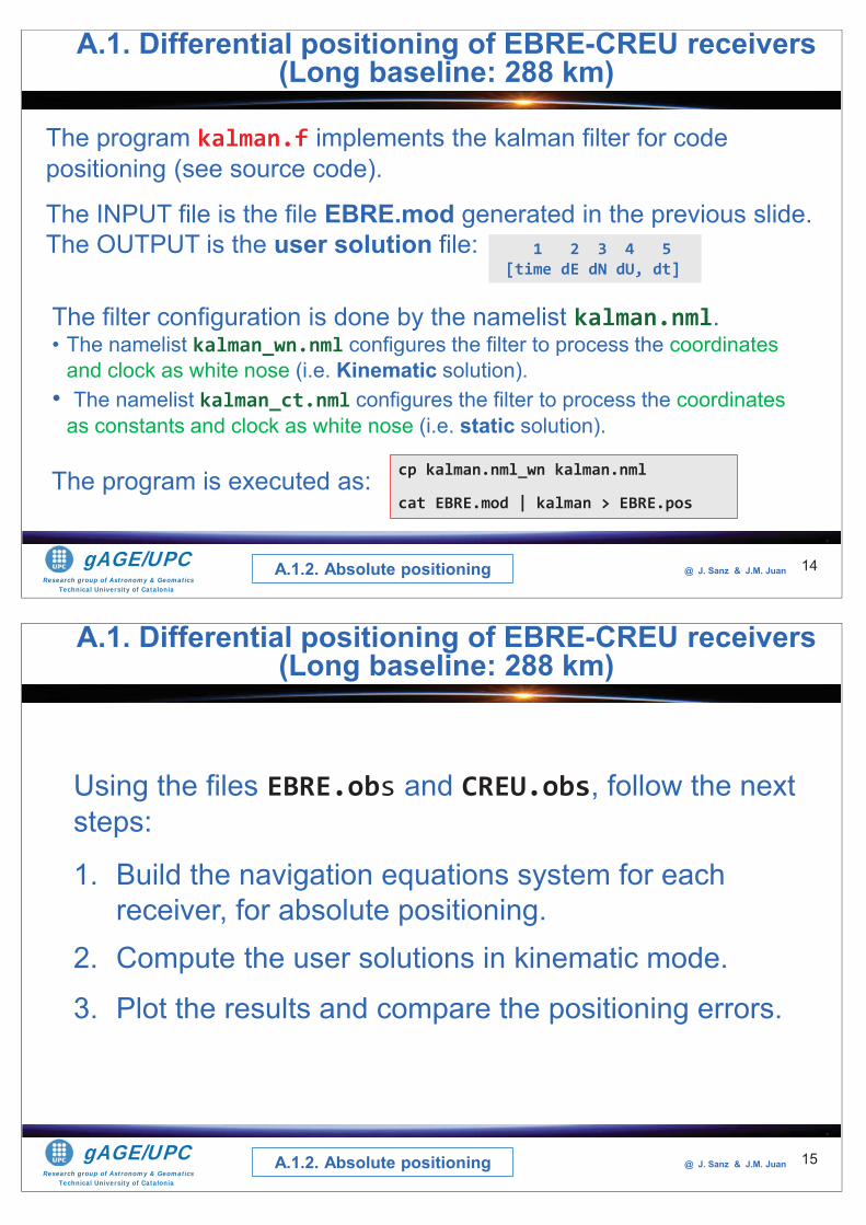
Research group of Astronomy & GeomaticsTechnical University of Catalonia
gAGE/UPC @ J. Sanz & J.M. Juan 14
The program kalman.f implements the kalman filter for code positioning (see source code).
The INPUT file is the file EBRE.mod generated in the previous slide. The OUTPUT is the user solution file: 1 2 3 4 5
[time dE dN dU, dt]
The filter configuration is done by the namelist kalman.nml.• The namelist kalman_wn.nml configures the filter to process the coordinates
and clock as white nose (i.e. Kinematic solution).• The namelist kalman_ct.nml configures the filter to process the coordinates
as constants and clock as white nose (i.e. static solution).
The program is executed as: cp kalman.nml_wn kalman.nml
cat EBRE.mod | kalman > EBRE.pos
A.1. Differential positioning of EBRE-CREU receivers (Long baseline: 288 km)
A.1.2. Absolute positioning
Research group of Astronomy & GeomaticsTechnical University of Catalonia
gAGE/UPC @ J. Sanz & J.M. Juan 15
Using the files EBRE.obs and CREU.obs, follow the next steps:
1. Build the navigation equations system for each receiver, for absolute positioning.
2. Compute the user solutions in kinematic mode.
3. Plot the results and compare the positioning errors.
A.1. Differential positioning of EBRE-CREU receivers (Long baseline: 288 km)
A.1.2. Absolute positioning

Research group of Astronomy & GeomaticsTechnical University of Catalonia
gAGE/UPC @ J. Sanz & J.M. Juan
2.- Computing the user solution for absolute positioning:
16
cp kalman.nml_wn kalman.nml
cat EBRE.mod | kalman > EBRE.pos
3.- Plotting results:graph.py -f EBRE.pos -x1 -y2 -s.- -l "North error"
-f EBRE.pos -x1 -y3 -s.- -l "East error" -f EBRE.pos -x1 -y4 -s.- -l "UP error" --xl "time (s)" --yl "error (m)" --yn -8 --yx 8 -t "EBRE: Standard Point Positioning"
1.- Building the navigation equations system for absolute positioning: cat EBRE.obs | gawk 'BEGIN{g2r=atan2(1,1)/45}{e=$12*g2r;a=$13*g2r;
printf "%8.2f %8.4f %8.4f %8.4f %8.4f %1i \n",$4, $14 ,-cos(e)*sin(a),-cos(e)*cos(a),-sin(e),1 }'> EBRE.mod
A.1. Differential positioning of EBRE-CREU receivers (Long baseline: 288 km)
A.1.2. Absolute positioning
Research group of Astronomy & GeomaticsTechnical University of Catalonia
gAGE/UPC @ J. Sanz & J.M. Juan
2.- Computing the user solution for absolute positioning:
17
cp kalman.nml_wn kalman.nml
cat CREU.mod | kalman > CREU.pos
3.- Plotting results:graph.py -f CREU.pos -x1 -y2 -s.- -l "North error"
-f CREU.pos -x1 -y3 -s.- -l "East error" -f CREU.pos -x1 -y4 -s.- -l "UP error" --xl "time (s)" --yl "error (m)" --yn -8 --yx 8 -t "CREU: Standard Point Positioning"
1.- Building the navigation equations system for absolute positioning: cat CREU.obs | gawk 'BEGIN{g2r=atan2(1,1)/45}{e=$12*g2r;a=$13*g2r;
printf "%8.2f %8.4f %8.4f %8.4f %8.4f %1i \n",$4, $14 ,-cos(e)*sin(a),-cos(e)*cos(a),-sin(e),1 }'> CREU.mod
A.1. Differential positioning of EBRE-CREU receivers (Long baseline: 288 km)
A.1.2. Absolute positioning
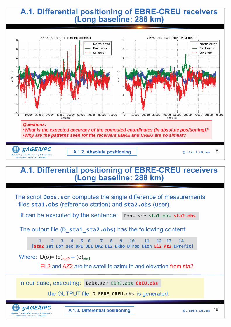
Research group of Astronomy & GeomaticsTechnical University of Catalonia
gAGE/UPC @ J. Sanz & J.M. Juan 18
A.1. Differential positioning of EBRE-CREU receivers (Long baseline: 288 km)
A.1.2. Absolute positioning
Questions: •What is the expected accuracy of the computed coordinates (in absolute positioning)?•Why are the patterns seen for the receivers EBRE and CREU are so similar?
Research group of Astronomy & GeomaticsTechnical University of Catalonia
gAGE/UPC @ J. Sanz & J.M. Juan
The script Dobs.scr computes the single difference of measurementsfiles sta1.obs (reference station) and sta2.obs (user).
19
The output file (D_sta1_sta2.obs) has the following content:
1 2 3 4 5 6 7 8 9 10 11 12 13 14[sta2 sat DoY sec DP1 DL1 DP2 DL2 DRho DTrop DIon El2 Az2 DPrefit]
It can be executed by the sentence: Dobs.scr sta1.obs sta2.obs
Where: D(o)= (o)sta2 -- (o)sta1
EL2 and AZ2 are the satellite azimuth and elevation from sta2.
In our case, executing: Dobs.scr EBRE.obs CREU.obs
the OUTPUT file is generated. D_EBRE_CREU.obs
A.1. Differential positioning of EBRE-CREU receivers (Long baseline: 288 km)
A.1.3. Differential positioning
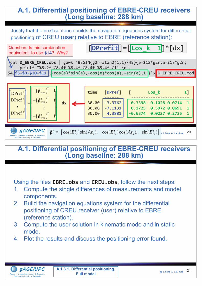
Research group of Astronomy & GeomaticsTechnical University of Catalonia
gAGE/UPC @ J. Sanz & J.M. Juan 20
cat D_EBRE_CREU.obs | gawk 'BEGIN{g2r=atan2(1,1)/45}{e=$12*g2r;a=$13*g2r;printf "%8.2f %8.4f %8.4f %8.4f %8.4f %1i \n",
$4,$5-$9-$10-$11 ,-cos(e)*sin(a),-cos(e)*cos(a),-sin(e),1 }'> D_EBRE_CREU.mod
Justify that the next sentence builds the navigation equations system for differential positioning of CREU (user) relative to EBRE (reference station):
[DPrefit]=[Los_k 1]*[dx]
11 creu
2 2creu
creu
ˆ 1DPrefˆDPref 1
DPref ˆ 1
T
T
n Tn
ρ
ρ dx
ρ
ˆ cos( )sin( ), cos( )cos( ), sin( )kk k k k kEl Az El Az Elρ
Question: Is this combination equivalent to use $14? Why?
A.1. Differential positioning of EBRE-CREU receivers (Long baseline: 288 km)
time [DPref] [ Los_k 1] ------ ------------------------
30.00 -3.3762 0.3398 -0.1028 0.0714 130.00 -7.1131 0.1725 0.5972 0.0691 1 30.00 4.3881 -0.6374 0.0227 0.2725 1
Research group of Astronomy & GeomaticsTechnical University of Catalonia
gAGE/UPC @ J. Sanz & J.M. Juan 21
Using the files EBRE.obs and CREU.obs, follow the next steps:1. Compute the single differences of measurements and model
components.2. Build the navigation equations system for the differential
positioning of CREU receiver (user) relative to EBRE (reference station).
3. Compute the user solution in kinematic mode and in static mode.
4. Plot the results and discuss the positioning error found.
A.1. Differential positioning of EBRE-CREU receivers (Long baseline: 288 km)
A.1.3.1. Differential positioning.Full model
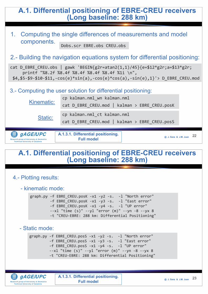
Research group of Astronomy & GeomaticsTechnical University of Catalonia
gAGE/UPC @ J. Sanz & J.M. Juan
3.- Computing the user solution for differential positioning:
22
cp kalman.nml_wn kalman.nmlcat D_EBRE_CREU.mod | kalman > EBRE_CREU.posK
2.- Building the navigation equations system for differential positioning: cat D_EBRE_CREU.obs | gawk 'BEGIN{g2r=atan2(1,1)/45}{e=$12*g2r;a=$13*g2r;
printf "%8.2f %8.4f %8.4f %8.4f %8.4f %1i \n",$4,$5-$9-$10-$11,-cos(e)*sin(a),-cos(e)*cos(a),-sin(e),1}'> D_EBRE_CREU.mod
1. Computing the single differences of measurements and model components.
Dobs.scr EBRE.obs CREU.obs
cp kalman.nml_ct kalman.nmlcat D_EBRE_CREU.mod | kalman > EBRE_CREU.posS
Kinematic:
Static:
A.1. Differential positioning of EBRE-CREU receivers (Long baseline: 288 km)
A.1.3.1. Differential positioning.Full model
Research group of Astronomy & GeomaticsTechnical University of Catalonia
gAGE/UPC @ J. Sanz & J.M. Juan 23
4.- Plotting results:
- kinematic mode:graph.py -f EBRE_CREU.posK -x1 -y2 -s. -l "North error"
-f EBRE_CREU.posK -x1 -y3 -s. -l "East error" -f EBRE_CREU.posK -x1 -y4 -s. -l "UP error" --xl "time (s)" --yl "error (m)" --yn -8 --yx 8 -t "CREU-EBRE: 288 km: Differential Positioning"
- Static mode:graph.py -f EBRE_CREU.posS -x1 -y2 -s. -l "North error"
-f EBRE_CREU.posS -x1 -y3 -s. -l "East error" -f EBRE_CREU.posS -x1 -y4 -s. -l "UP error" --xl "time (s)" --yl "error (m)" --yn -8 --yx 8 -t "CREU-EBRE: 288 km: Differential Positioning"
A.1. Differential positioning of EBRE-CREU receivers (Long baseline: 288 km)
A.1.3.1. Differential positioning.Full model
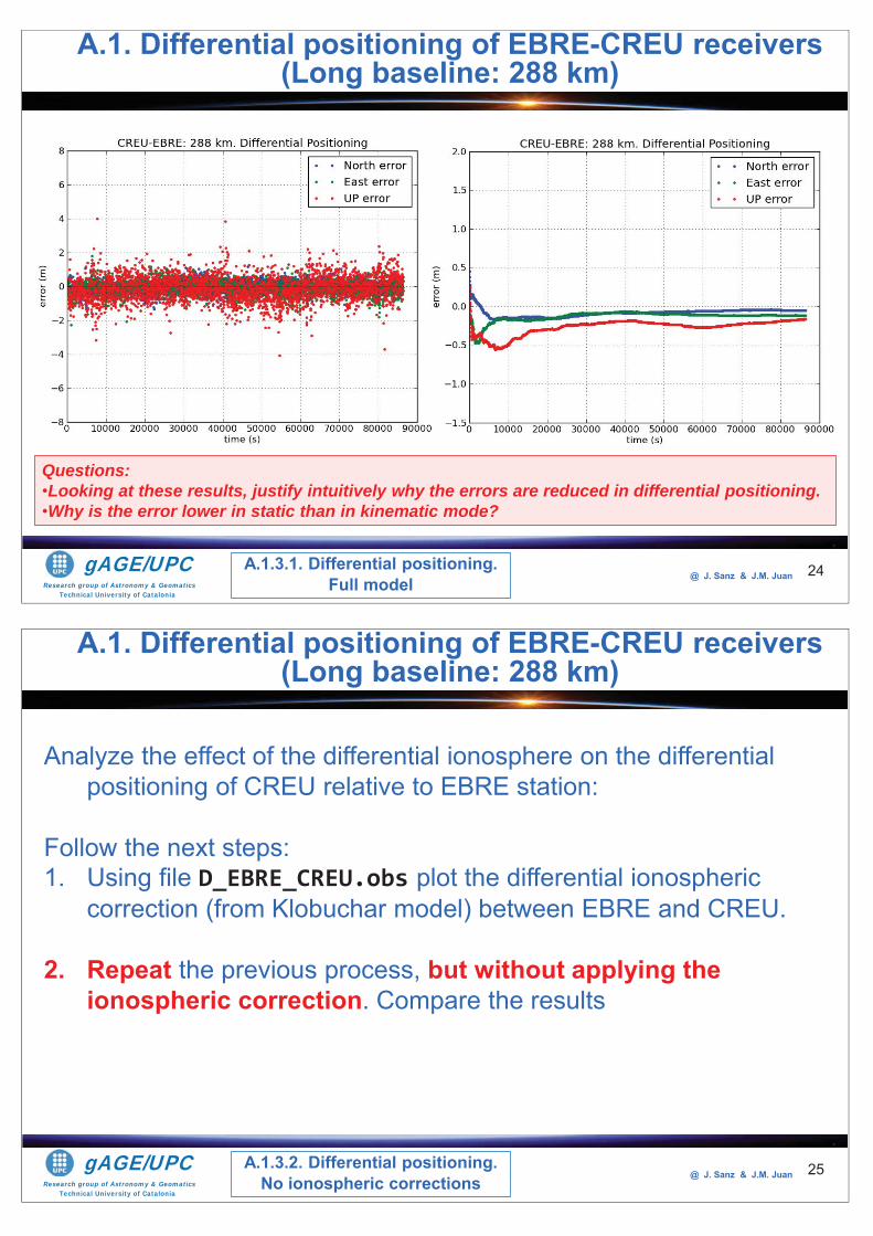
Research group of Astronomy & GeomaticsTechnical University of Catalonia
gAGE/UPC @ J. Sanz & J.M. Juan 24
A.1. Differential positioning of EBRE-CREU receivers (Long baseline: 288 km)
A.1.3.1. Differential positioning.Full model
Questions: •Looking at these results, justify intuitively why the errors are reduced in differential positioning.•Why is the error lower in static than in kinematic mode?
Research group of Astronomy & GeomaticsTechnical University of Catalonia
gAGE/UPC @ J. Sanz & J.M. Juan 25
Analyze the effect of the differential ionosphere on the differential positioning of CREU relative to EBRE station:
Follow the next steps:1. Using file D_EBRE_CREU.obs plot the differential ionospheric
correction (from Klobuchar model) between EBRE and CREU.
2. Repeat the previous process, but without applying the ionospheric correction. Compare the results
A.1. Differential positioning of EBRE-CREU receivers (Long baseline: 288 km)
A.1.3.2. Differential positioning.No ionospheric corrections
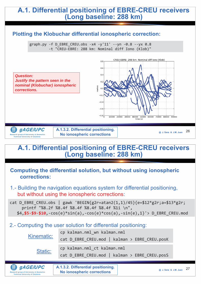
Research group of Astronomy & GeomaticsTechnical University of Catalonia
gAGE/UPC @ J. Sanz & J.M. Juan 26
Plotting the Klobuchar differential ionospheric correction:
graph.py -f D_EBRE_CREU.obs -x4 -y'11' --yn -0.8 --yx 0.8 -t "CREU-EBRE: 288 km: Nominal diff Iono (Klob)"
A.1. Differential positioning of EBRE-CREU receivers (Long baseline: 288 km)
A.1.3.2. Differential positioning.No ionospheric corrections
Question: Justify the pattern seen in the nominal (Klobuchar) ionospheric corrections.
Research group of Astronomy & GeomaticsTechnical University of Catalonia
gAGE/UPC @ J. Sanz & J.M. Juan
2.- Computing the user solution for differential positioning:
27
cp kalman.nml_wn kalman.nmlcat D_EBRE_CREU.mod | kalman > EBRE_CREU.posK
cat D_EBRE_CREU.obs | gawk 'BEGIN{g2r=atan2(1,1)/45}{e=$12*g2r;a=$13*g2r;printf "%8.2f %8.4f %8.4f %8.4f %8.4f %1i \n",
$4,$5-$9-$10,-cos(e)*sin(a),-cos(e)*cos(a),-sin(e),1}'> D_EBRE_CREU.mod
Computing the differential solution, but without using ionospheric corrections:
cp kalman.nml_ct kalman.nmlcat D_EBRE_CREU.mod | kalman > EBRE_CREU.posS
Kinematic:
Static:
1.- Building the navigation equations system for differential positioning, but without using the ionospheric corrections:
A.1. Differential positioning of EBRE-CREU receivers (Long baseline: 288 km)
A.1.3.2. Differential positioning.No ionospheric corrections
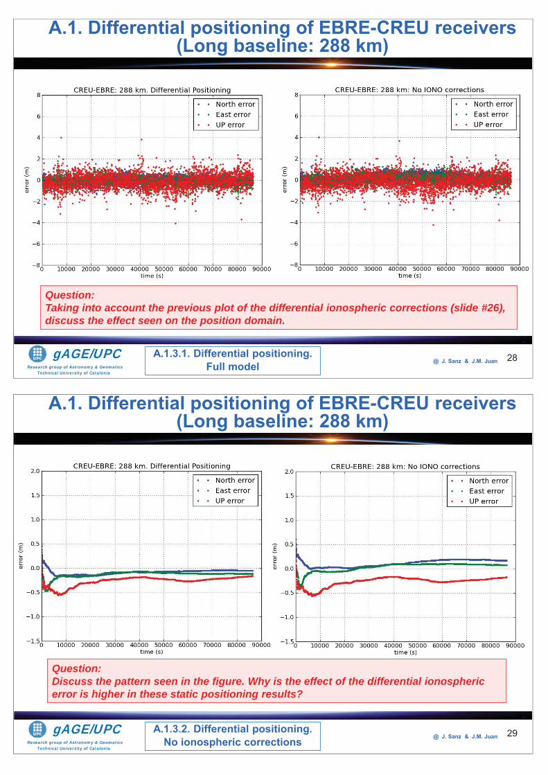
Research group of Astronomy & GeomaticsTechnical University of Catalonia
gAGE/UPC @ J. Sanz & J.M. Juan 28
A.1. Differential positioning of EBRE-CREU receivers (Long baseline: 288 km)
A.1.3.1. Differential positioning.Full model
Question: Taking into account the previous plot of the differential ionospheric corrections (slide #26), discuss the effect seen on the position domain.
Research group of Astronomy & GeomaticsTechnical University of Catalonia
gAGE/UPC @ J. Sanz & J.M. Juan 29
A.1. Differential positioning of EBRE-CREU receivers (Long baseline: 288 km)
A.1.3.2. Differential positioning.No ionospheric corrections
Question: Discuss the pattern seen in the figure. Why is the effect of the differential ionospheric error is higher in these static positioning results?
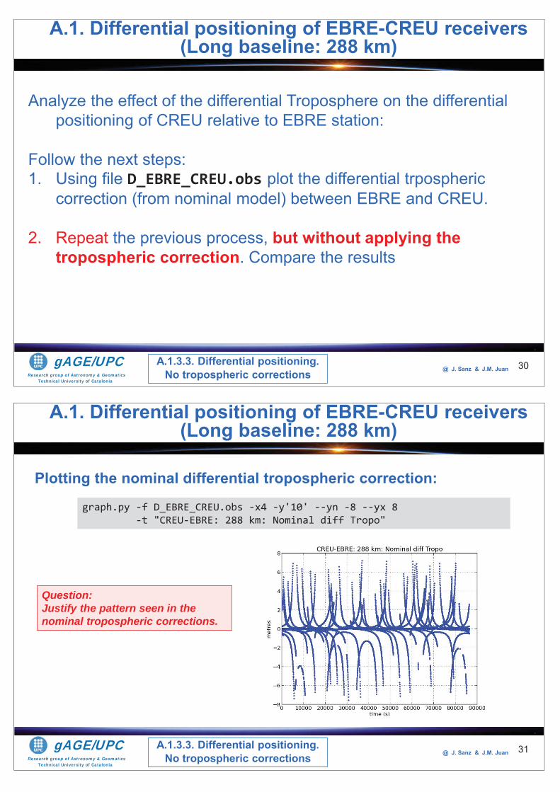
Research group of Astronomy & GeomaticsTechnical University of Catalonia
gAGE/UPC @ J. Sanz & J.M. Juan 30
Analyze the effect of the differential Troposphere on the differential positioning of CREU relative to EBRE station:
Follow the next steps:1. Using file D_EBRE_CREU.obs plot the differential trpospheric
correction (from nominal model) between EBRE and CREU.
2. Repeat the previous process, but without applying the tropospheric correction. Compare the results
A.1. Differential positioning of EBRE-CREU receivers (Long baseline: 288 km)
A.1.3.3. Differential positioning.No tropospheric corrections
Research group of Astronomy & GeomaticsTechnical University of Catalonia
gAGE/UPC @ J. Sanz & J.M. Juan 31
Plotting the nominal differential tropospheric correction:
graph.py -f D_EBRE_CREU.obs -x4 -y'10' --yn -8 --yx 8 -t "CREU-EBRE: 288 km: Nominal diff Tropo"
A.1. Differential positioning of EBRE-CREU receivers (Long baseline: 288 km)
A.1.3.3. Differential positioning.No tropospheric corrections
Question: Justify the pattern seen in the nominal tropospheric corrections.
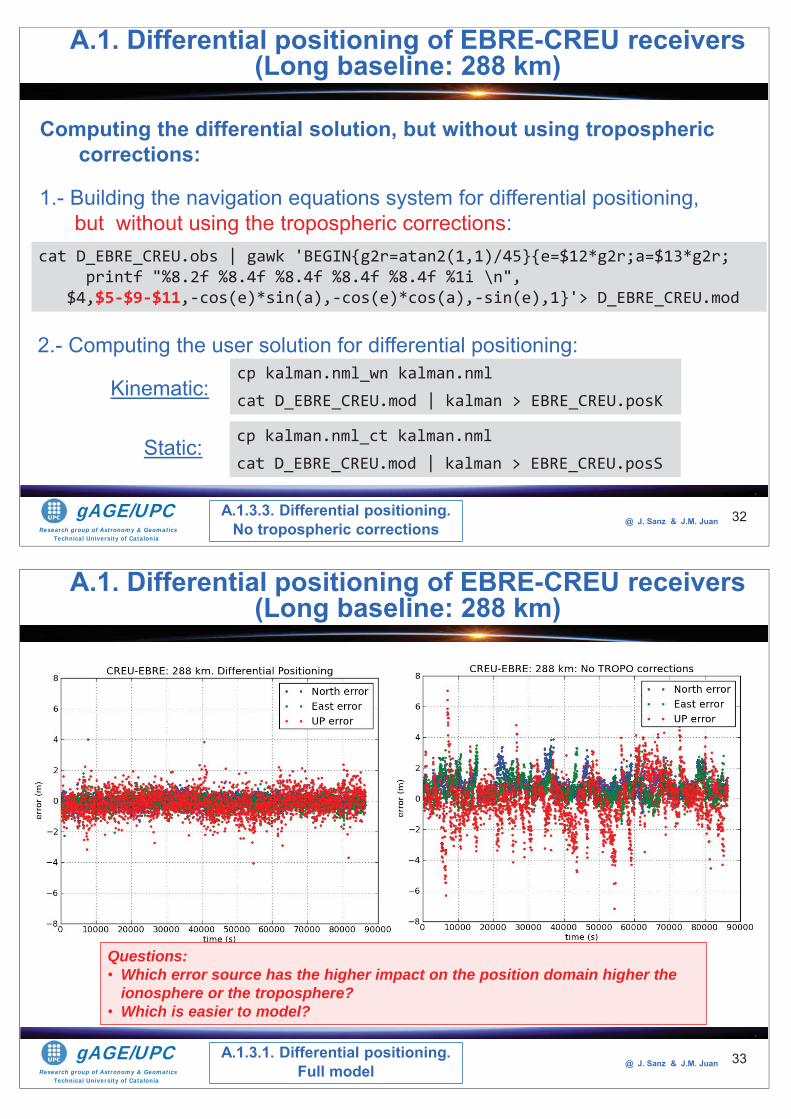
Research group of Astronomy & GeomaticsTechnical University of Catalonia
gAGE/UPC @ J. Sanz & J.M. Juan
2.- Computing the user solution for differential positioning:
32
cp kalman.nml_wn kalman.nmlcat D_EBRE_CREU.mod | kalman > EBRE_CREU.posK
cat D_EBRE_CREU.obs | gawk 'BEGIN{g2r=atan2(1,1)/45}{e=$12*g2r;a=$13*g2r;printf "%8.2f %8.4f %8.4f %8.4f %8.4f %1i \n",
$4,$5-$9-$11,-cos(e)*sin(a),-cos(e)*cos(a),-sin(e),1}'> D_EBRE_CREU.mod
Computing the differential solution, but without using tropospheric corrections:
cp kalman.nml_ct kalman.nmlcat D_EBRE_CREU.mod | kalman > EBRE_CREU.posS
Kinematic:
Static:
1.- Building the navigation equations system for differential positioning, but without using the tropospheric corrections:
A.1. Differential positioning of EBRE-CREU receivers (Long baseline: 288 km)
A.1.3.3. Differential positioning.No tropospheric corrections
Research group of Astronomy & GeomaticsTechnical University of Catalonia
gAGE/UPC @ J. Sanz & J.M. Juan 33
A.1. Differential positioning of EBRE-CREU receivers (Long baseline: 288 km)
A.1.3.1. Differential positioning.Full model
Questions: • Which error source has the higher impact on the position domain higher the
ionosphere or the troposphere?• Which is easier to model?
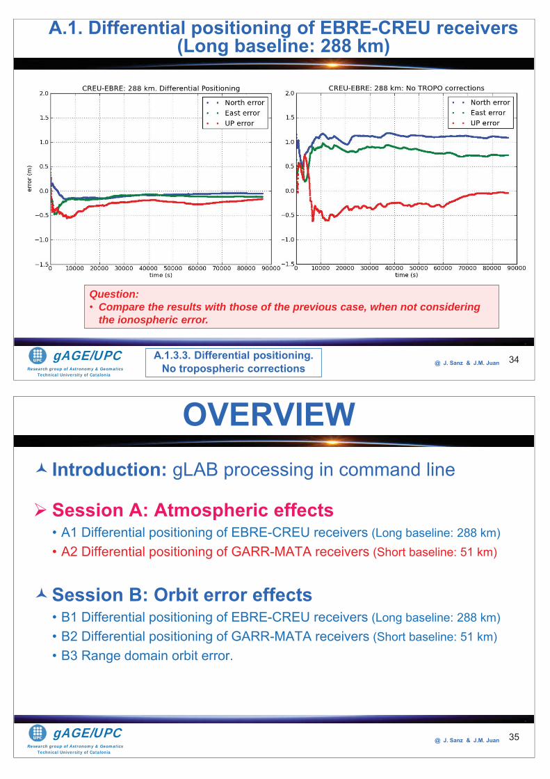
Research group of Astronomy & GeomaticsTechnical University of Catalonia
gAGE/UPC @ J. Sanz & J.M. Juan 34
A.1. Differential positioning of EBRE-CREU receivers (Long baseline: 288 km)
A.1.3.3. Differential positioning.No tropospheric corrections
Question: • Compare the results with those of the previous case, when not considering
the ionospheric error.
Research group of Astronomy & GeomaticsTechnical University of Catalonia
gAGE/UPC @ J. Sanz & J.M. Juan
Introduction: gLAB processing in command line
Session A: Atmospheric effects• A1 Differential positioning of EBRE-CREU receivers (Long baseline: 288 km) • A2 Differential positioning of GARR-MATA receivers (Short baseline: 51 km)
Session B: Orbit error effects• B1 Differential positioning of EBRE-CREU receivers (Long baseline: 288 km) • B2 Differential positioning of GARR-MATA receivers (Short baseline: 51 km)• B3 Range domain orbit error.
OVERVIEW
35
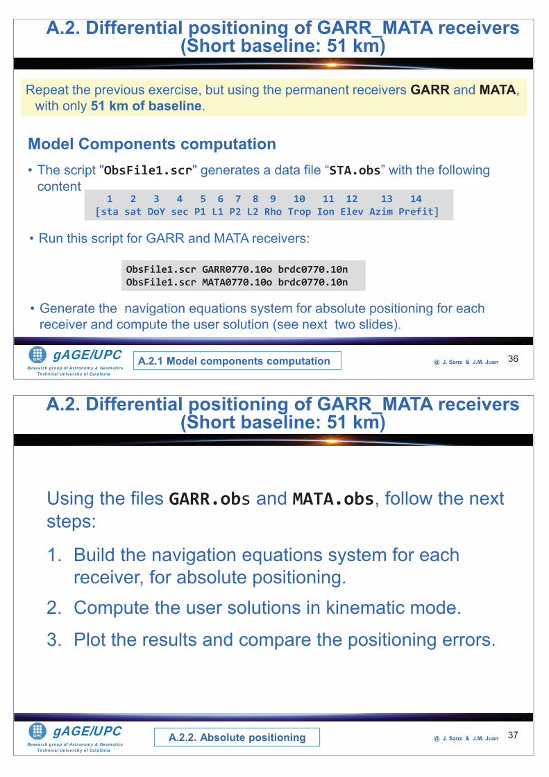
Research group of Astronomy & GeomaticsTechnical University of Catalonia
gAGE/UPC @ J. Sanz & J.M. Juan
Model Components computation• The script "ObsFile1.scr" generates a data file “STA.obs” with the following
content
36
1 2 3 4 5 6 7 8 9 10 11 12 13 14[sta sat DoY sec P1 L1 P2 L2 Rho Trop Ion Elev Azim Prefit]
• Run this script for GARR and MATA receivers:
ObsFile1.scr GARR0770.10o brdc0770.10nObsFile1.scr MATA0770.10o brdc0770.10n
• Generate the navigation equations system for absolute positioning for each receiver and compute the user solution (see next two slides).
A.2.1 Model components computation
A.2. Differential positioning of GARR_MATA receivers (Short baseline: 51 km)
Repeat the previous exercise, but using the permanent receivers GARR and MATA, with only 51 km of baseline.
Research group of Astronomy & GeomaticsTechnical University of Catalonia
gAGE/UPC @ J. Sanz & J.M. Juan 37
Using the files GARR.obs and MATA.obs, follow the next steps:
1. Build the navigation equations system for each receiver, for absolute positioning.
2. Compute the user solutions in kinematic mode.
3. Plot the results and compare the positioning errors.
A.2.2. Absolute positioning
A.2. Differential positioning of GARR_MATA receivers (Short baseline: 51 km)
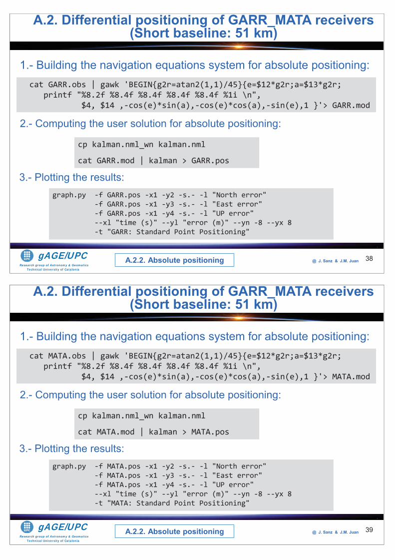
Research group of Astronomy & GeomaticsTechnical University of Catalonia
gAGE/UPC @ J. Sanz & J.M. Juan
2.- Computing the user solution for absolute positioning:
38
cp kalman.nml_wn kalman.nml
cat GARR.mod | kalman > GARR.pos
3.- Plotting the results:graph.py -f GARR.pos -x1 -y2 -s.- -l "North error"
-f GARR.pos -x1 -y3 -s.- -l "East error" -f GARR.pos -x1 -y4 -s.- -l "UP error" --xl "time (s)" --yl "error (m)" --yn -8 --yx 8 -t "GARR: Standard Point Positioning"
1.- Building the navigation equations system for absolute positioning: cat GARR.obs | gawk 'BEGIN{g2r=atan2(1,1)/45}{e=$12*g2r;a=$13*g2r;
printf "%8.2f %8.4f %8.4f %8.4f %8.4f %1i \n",$4, $14 ,-cos(e)*sin(a),-cos(e)*cos(a),-sin(e),1 }'> GARR.mod
A.2.2. Absolute positioning
A.2. Differential positioning of GARR_MATA receivers (Short baseline: 51 km)
Research group of Astronomy & GeomaticsTechnical University of Catalonia
gAGE/UPC @ J. Sanz & J.M. Juan
2.- Computing the user solution for absolute positioning:
39
cp kalman.nml_wn kalman.nml
cat MATA.mod | kalman > MATA.pos
3.- Plotting the results:graph.py -f MATA.pos -x1 -y2 -s.- -l "North error"
-f MATA.pos -x1 -y3 -s.- -l "East error" -f MATA.pos -x1 -y4 -s.- -l "UP error" --xl "time (s)" --yl "error (m)" --yn -8 --yx 8 -t "MATA: Standard Point Positioning"
1.- Building the navigation equations system for absolute positioning: cat MATA.obs | gawk 'BEGIN{g2r=atan2(1,1)/45}{e=$12*g2r;a=$13*g2r;
printf "%8.2f %8.4f %8.4f %8.4f %8.4f %1i \n",$4, $14 ,-cos(e)*sin(a),-cos(e)*cos(a),-sin(e),1 }'> MATA.mod
A.2.2. Absolute positioning
A.2. Differential positioning of GARR_MATA receivers (Short baseline: 51 km)
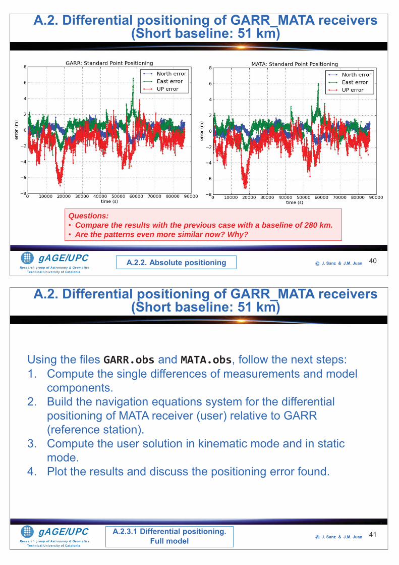
Research group of Astronomy & GeomaticsTechnical University of Catalonia
gAGE/UPC @ J. Sanz & J.M. Juan 40A.2.2. Absolute positioning
A.2. Differential positioning of GARR_MATA receivers (Short baseline: 51 km)
Questions: • Compare the results with the previous case with a baseline of 280 km.• Are the patterns even more similar now? Why?
Research group of Astronomy & GeomaticsTechnical University of Catalonia
gAGE/UPC @ J. Sanz & J.M. Juan 41
Using the files GARR.obs and MATA.obs, follow the next steps:1. Compute the single differences of measurements and model
components.2. Build the navigation equations system for the differential
positioning of MATA receiver (user) relative to GARR (reference station).
3. Compute the user solution in kinematic mode and in static mode.
4. Plot the results and discuss the positioning error found.
A.2.3.1 Differential positioning.Full model
A.2. Differential positioning of GARR_MATA receivers (Short baseline: 51 km)
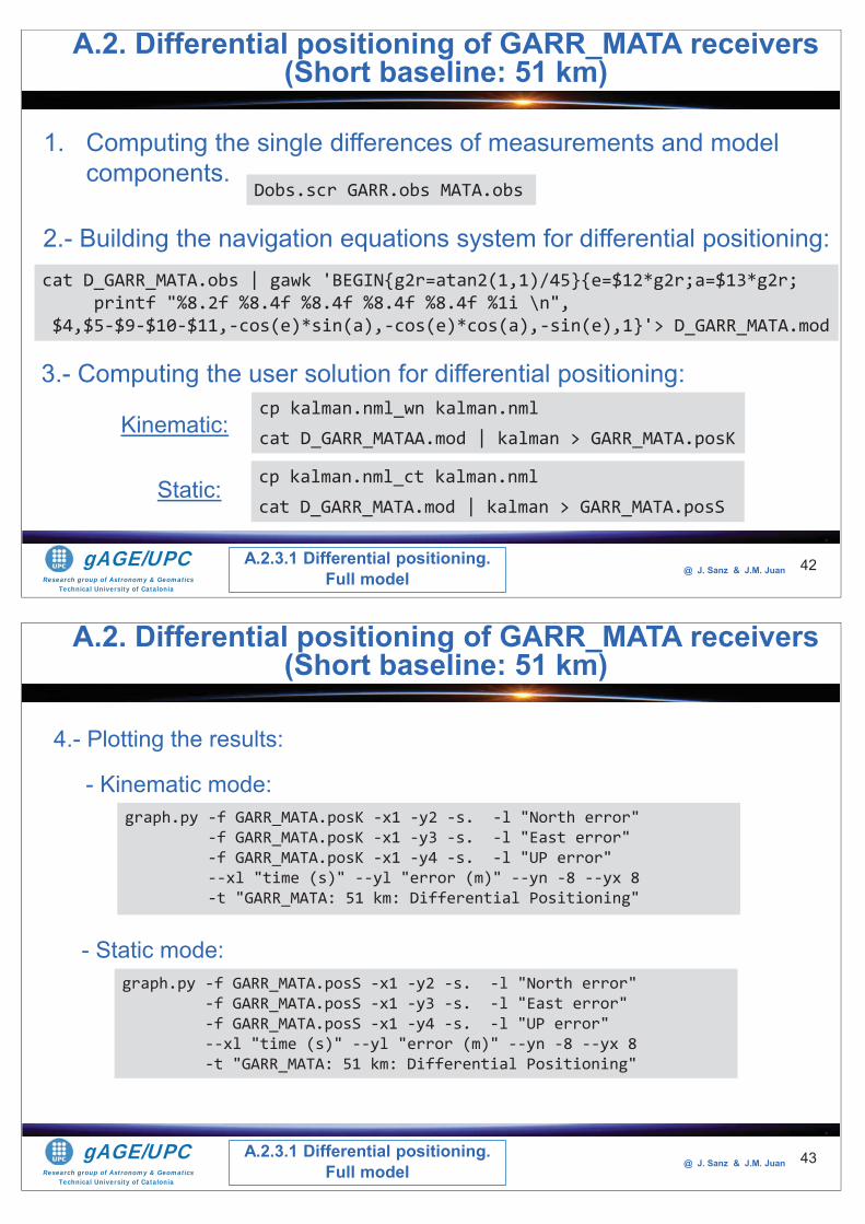
Research group of Astronomy & GeomaticsTechnical University of Catalonia
gAGE/UPC @ J. Sanz & J.M. Juan
3.- Computing the user solution for differential positioning:
42
cp kalman.nml_wn kalman.nmlcat D_GARR_MATAA.mod | kalman > GARR_MATA.posK
2.- Building the navigation equations system for differential positioning: cat D_GARR_MATA.obs | gawk 'BEGIN{g2r=atan2(1,1)/45}{e=$12*g2r;a=$13*g2r;
printf "%8.2f %8.4f %8.4f %8.4f %8.4f %1i \n",$4,$5-$9-$10-$11,-cos(e)*sin(a),-cos(e)*cos(a),-sin(e),1}'> D_GARR_MATA.mod
1. Computing the single differences of measurements and model components.
Dobs.scr GARR.obs MATA.obs
cp kalman.nml_ct kalman.nmlcat D_GARR_MATA.mod | kalman > GARR_MATA.posS
Kinematic:
Static:
A.2.3.1 Differential positioning.Full model
A.2. Differential positioning of GARR_MATA receivers (Short baseline: 51 km)
Research group of Astronomy & GeomaticsTechnical University of Catalonia
gAGE/UPC @ J. Sanz & J.M. Juan 43
4.- Plotting the results:
- Kinematic mode:graph.py -f GARR_MATA.posK -x1 -y2 -s. -l "North error"
-f GARR_MATA.posK -x1 -y3 -s. -l "East error" -f GARR_MATA.posK -x1 -y4 -s. -l "UP error" --xl "time (s)" --yl "error (m)" --yn -8 --yx 8 -t "GARR_MATA: 51 km: Differential Positioning"
- Static mode:graph.py -f GARR_MATA.posS -x1 -y2 -s. -l "North error"
-f GARR_MATA.posS -x1 -y3 -s. -l "East error" -f GARR_MATA.posS -x1 -y4 -s. -l "UP error" --xl "time (s)" --yl "error (m)" --yn -8 --yx 8 -t "GARR_MATA: 51 km: Differential Positioning"
A.2.3.1 Differential positioning.Full model
A.2. Differential positioning of GARR_MATA receivers (Short baseline: 51 km)
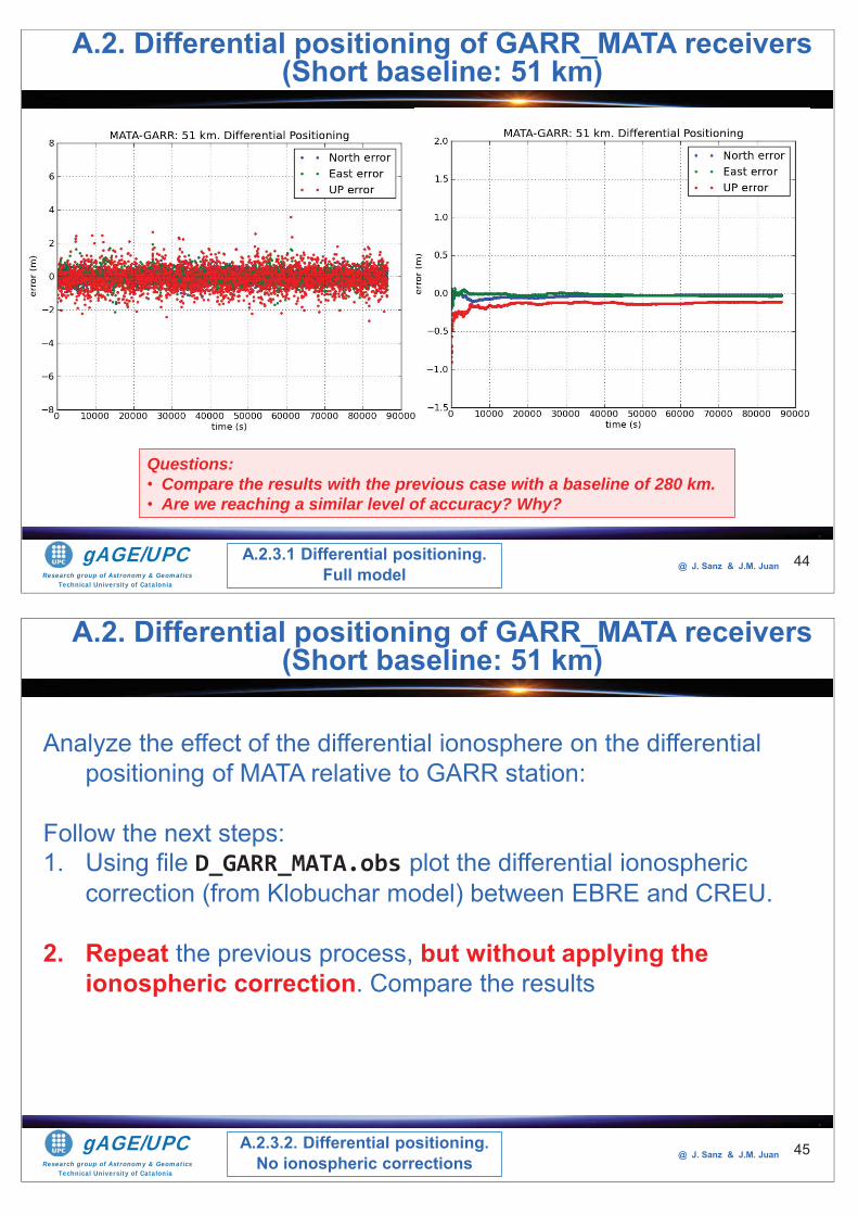
Research group of Astronomy & GeomaticsTechnical University of Catalonia
gAGE/UPC @ J. Sanz & J.M. Juan 44A.2.3.1 Differential positioning.
Full model
A.2. Differential positioning of GARR_MATA receivers (Short baseline: 51 km)
Questions: • Compare the results with the previous case with a baseline of 280 km.• Are we reaching a similar level of accuracy? Why?
Research group of Astronomy & GeomaticsTechnical University of Catalonia
gAGE/UPC @ J. Sanz & J.M. Juan 45
Analyze the effect of the differential ionosphere on the differential positioning of MATA relative to GARR station:
Follow the next steps:1. Using file D_GARR_MATA.obs plot the differential ionospheric
correction (from Klobuchar model) between EBRE and CREU.
2. Repeat the previous process, but without applying the ionospheric correction. Compare the results
A.2.3.2. Differential positioning.No ionospheric corrections
A.2. Differential positioning of GARR_MATA receivers (Short baseline: 51 km)
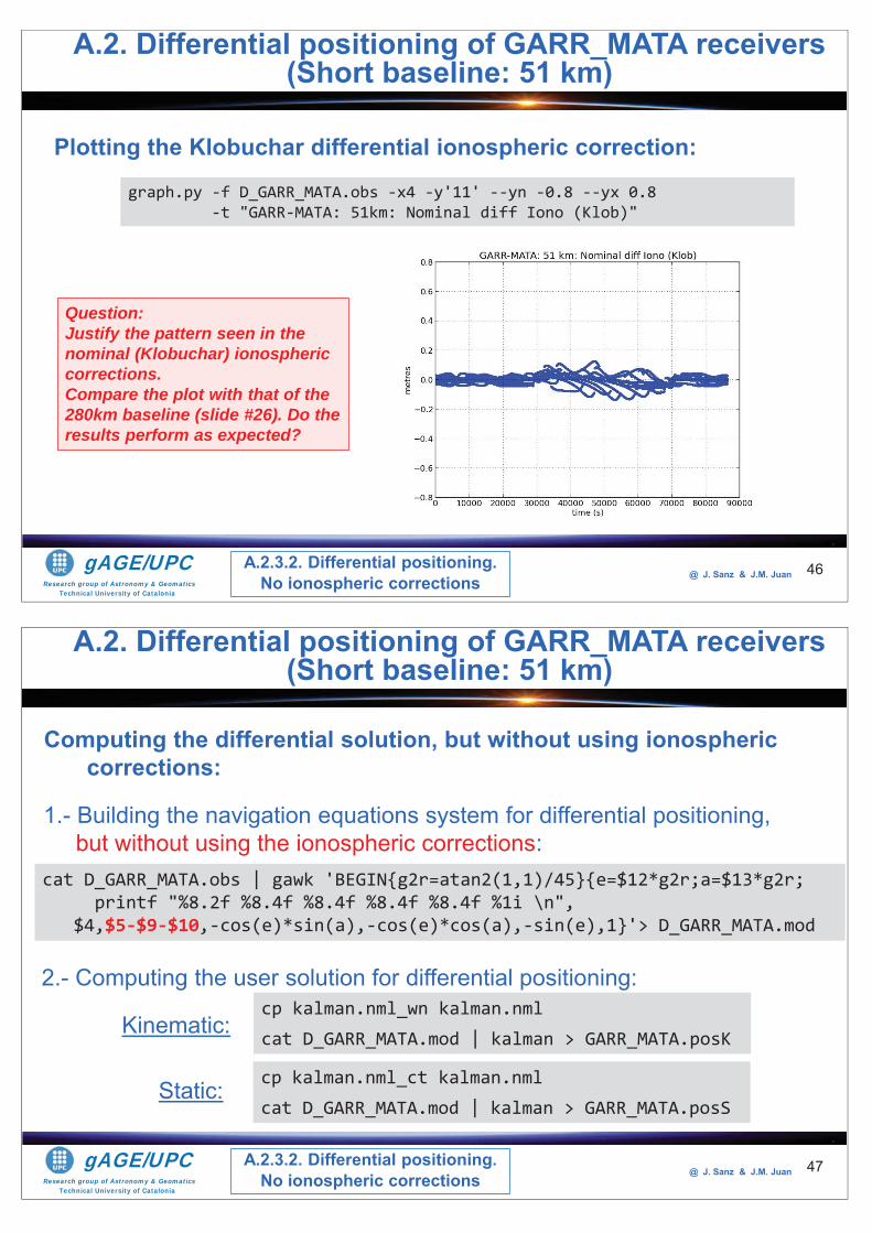
Research group of Astronomy & GeomaticsTechnical University of Catalonia
gAGE/UPC @ J. Sanz & J.M. Juan 46
Plotting the Klobuchar differential ionospheric correction:
graph.py -f D_GARR_MATA.obs -x4 -y'11' --yn -0.8 --yx 0.8 -t "GARR-MATA: 51km: Nominal diff Iono (Klob)"
A.2. Differential positioning of GARR_MATA receivers (Short baseline: 51 km)
A.2.3.2. Differential positioning.No ionospheric corrections
Question: Justify the pattern seen in the nominal (Klobuchar) ionospheric corrections.Compare the plot with that of the 280km baseline (slide #26). Do the results perform as expected?
Research group of Astronomy & GeomaticsTechnical University of Catalonia
gAGE/UPC @ J. Sanz & J.M. Juan
2.- Computing the user solution for differential positioning:
47
cp kalman.nml_wn kalman.nmlcat D_GARR_MATA.mod | kalman > GARR_MATA.posK
cat D_GARR_MATA.obs | gawk 'BEGIN{g2r=atan2(1,1)/45}{e=$12*g2r;a=$13*g2r;printf "%8.2f %8.4f %8.4f %8.4f %8.4f %1i \n",
$4,$5-$9-$10,-cos(e)*sin(a),-cos(e)*cos(a),-sin(e),1}'> D_GARR_MATA.mod
Computing the differential solution, but without using ionospheric corrections:
cp kalman.nml_ct kalman.nmlcat D_GARR_MATA.mod | kalman > GARR_MATA.posS
Kinematic:
Static:
1.- Building the navigation equations system for differential positioning, but without using the ionospheric corrections:
A.2.3.2. Differential positioning.No ionospheric corrections
A.2. Differential positioning of GARR_MATA receivers (Short baseline: 51 km)
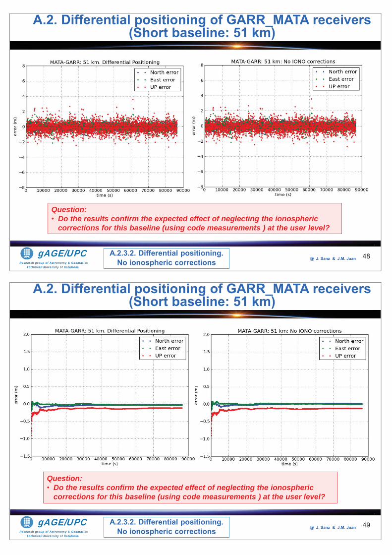
Research group of Astronomy & GeomaticsTechnical University of Catalonia
gAGE/UPC @ J. Sanz & J.M. Juan 48
A.2. Differential positioning of GARR_MATA receivers (Short baseline: 51 km)
A.2.3.2. Differential positioning.No ionospheric corrections
Question: • Do the results confirm the expected effect of neglecting the ionospheric
corrections for this baseline (using code measurements ) at the user level?
Research group of Astronomy & GeomaticsTechnical University of Catalonia
gAGE/UPC @ J. Sanz & J.M. Juan 49A.2.3.2. Differential positioning.
No ionospheric corrections
A.2. Differential positioning of GARR_MATA receivers (Short baseline: 51 km)
Question: • Do the results confirm the expected effect of neglecting the ionospheric
corrections for this baseline (using code measurements ) at the user level?
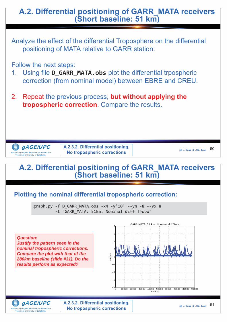
Research group of Astronomy & GeomaticsTechnical University of Catalonia
gAGE/UPC @ J. Sanz & J.M. Juan 50
Analyze the effect of the differential Troposphere on the differential positioning of MATA relative to GARR station:
Follow the next steps:1. Using file D_GARR_MATA.obs plot the differential trpospheric
correction (from nominal model) between EBRE and CREU.
2. Repeat the previous process, but without applying the tropospheric correction. Compare the results.
A.2.3.2. Differential positioning.No tropospheric corrections
A.2. Differential positioning of GARR_MATA receivers (Short baseline: 51 km)
Research group of Astronomy & GeomaticsTechnical University of Catalonia
gAGE/UPC @ J. Sanz & J.M. Juan 51
Plotting the nominal differential tropospheric correction:
graph.py -f D_GARR_MATA.obs -x4 -y'10' --yn -8 --yx 8 -t "GARR_MATA: 51km: Nominal diff Tropo"
A.2. Differential positioning of GARR_MATA receivers (Short baseline: 51 km)
A.2.3.2. Differential positioning.No tropospheric corrections
Question: Justify the pattern seen in the nominal tropospheric corrections.Compare the plot with that of the 280km baseline (slide #31). Do the results perform as expected?
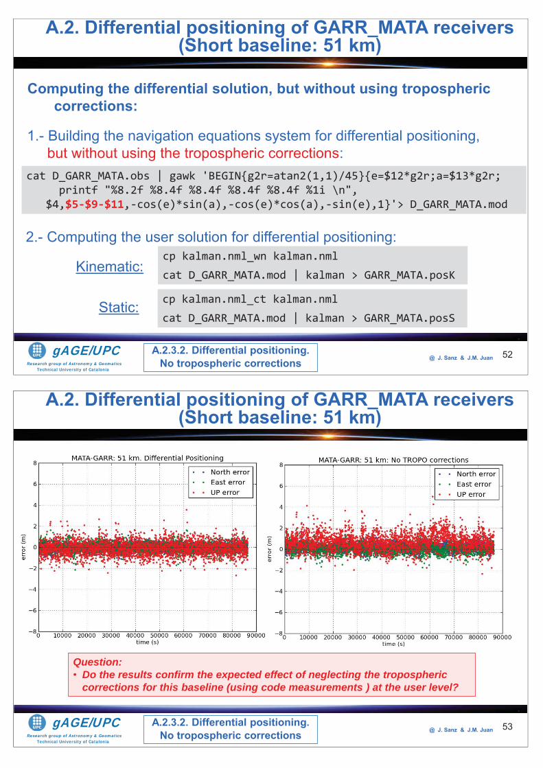
Research group of Astronomy & GeomaticsTechnical University of Catalonia
gAGE/UPC @ J. Sanz & J.M. Juan
2.- Computing the user solution for differential positioning:
52
cp kalman.nml_wn kalman.nmlcat D_GARR_MATA.mod | kalman > GARR_MATA.posK
cat D_GARR_MATA.obs | gawk 'BEGIN{g2r=atan2(1,1)/45}{e=$12*g2r;a=$13*g2r;printf "%8.2f %8.4f %8.4f %8.4f %8.4f %1i \n",
$4,$5-$9-$11,-cos(e)*sin(a),-cos(e)*cos(a),-sin(e),1}'> D_GARR_MATA.mod
Computing the differential solution, but without using tropospheric corrections:
cp kalman.nml_ct kalman.nmlcat D_GARR_MATA.mod | kalman > GARR_MATA.posS
Kinematic:
Static:
1.- Building the navigation equations system for differential positioning, but without using the tropospheric corrections:
A.2. Differential positioning of GARR_MATA receivers (Short baseline: 51 km)
A.2.3.2. Differential positioning.No tropospheric corrections
Research group of Astronomy & GeomaticsTechnical University of Catalonia
gAGE/UPC @ J. Sanz & J.M. Juan 53
A.2. Differential positioning of GARR_MATA receivers (Short baseline: 51 km)
A.2.3.2. Differential positioning.No tropospheric corrections
Question: • Do the results confirm the expected effect of neglecting the tropospheric
corrections for this baseline (using code measurements ) at the user level?
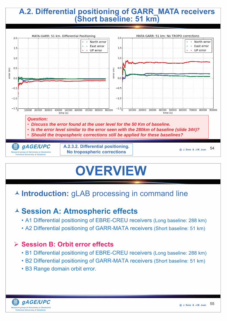
Research group of Astronomy & GeomaticsTechnical University of Catalonia
gAGE/UPC @ J. Sanz & J.M. Juan 54
A.2. Differential positioning of GARR_MATA receivers (Short baseline: 51 km)
A.2.3.2. Differential positioning.No tropospheric corrections
Question: • Discuss the error found at the user level for the 50 Km of baseline. • Is the error level similar to the error seen with the 280km of baseline (slide 34#)?• Should the tropospheric corrections still be applied for these baselines?
Research group of Astronomy & GeomaticsTechnical University of Catalonia
gAGE/UPC @ J. Sanz & J.M. Juan
Introduction: gLAB processing in command line
Session A: Atmospheric effects• A1 Differential positioning of EBRE-CREU receivers (Long baseline: 288 km) • A2 Differential positioning of GARR-MATA receivers (Short baseline: 51 km)
Session B: Orbit error effects• B1 Differential positioning of EBRE-CREU receivers (Long baseline: 288 km) • B2 Differential positioning of GARR-MATA receivers (Short baseline: 51 km)• B3 Range domain orbit error.
OVERVIEW
55
Research group of Astronomy & GeomaticsTechnical University of Catalonia
gAGE/UPC @ J. Sanz & J.M. Juan 56
Session B
Differential positioningOrbit errors
Research group of Astronomy & GeomaticsTechnical University of Catalonia
gAGE/UPC @ J. Sanz & J.M. Juan 57
The target of this exercise is to asses the satellite orbit error on absolute and differential positioning.
This will be done by modifying the broadcast orbit parameters to generate an Along-track orbit error of about 2000m and, positioning two receivers with these corrupted orbits.
The user positioning error using the original and the corrupted orbits will be compared for absolute and differential positioning, with the receivers and baselines used in the previous session.
B. Differential positioning.Orbit error
B. Orbit error effect on Differential positioning.
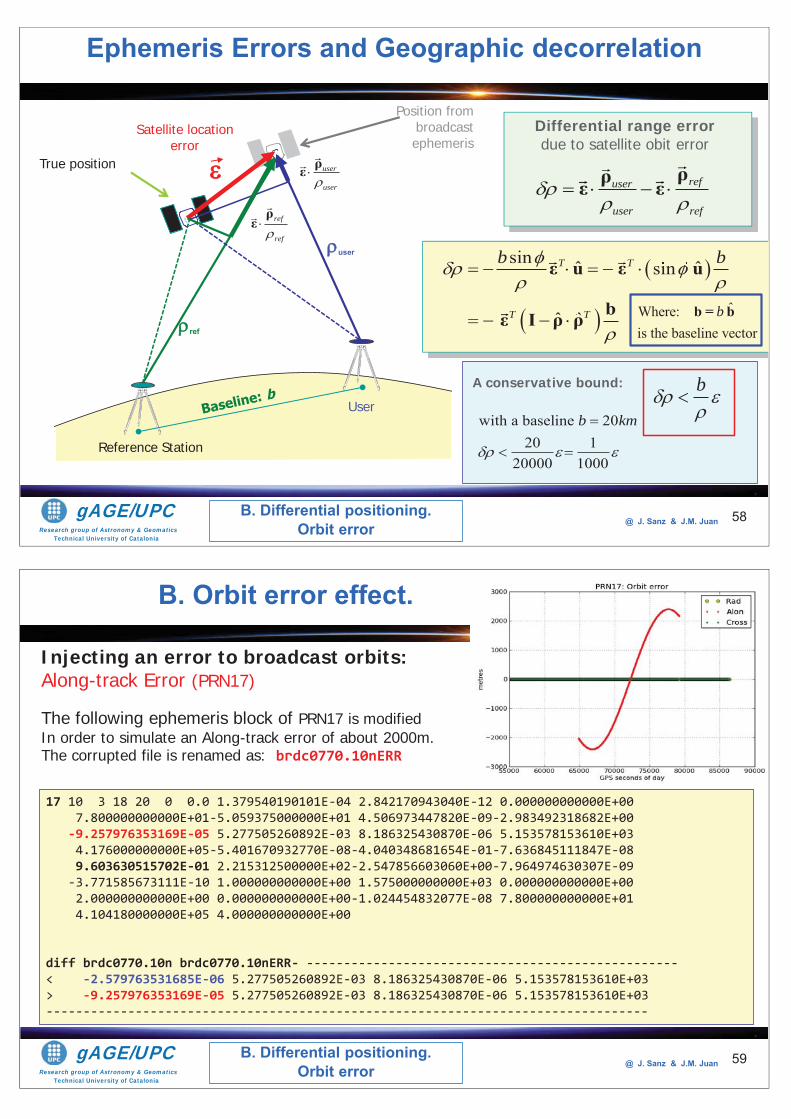
Research group of Astronomy & GeomaticsTechnical University of Catalonia
gAGE/UPC @ J. Sanz & J.M. Juan 58
True position
Reference Station
Ephemeris Errors and Geographic decorrelation
Satellite location error
Position from broadcast ephemeris
User
ref
user
user
ρε
ref
ref
ρε
user
refuser
user ref
ρρε ε
Differential range error due to satellite obit error
with a baseline 2020 1
20000 1000
b km
A conservative bound: b
sin ˆ ˆsin
ˆ ˆ
ˆ ˆˆ sin
ˆ ˆ
T T
T T
b bε u ε u
bε I ρ ρˆWhere:
is the baseline vectorbb = b
B. Differential positioning.Orbit error
Research group of Astronomy & GeomaticsTechnical University of Catalonia
gAGE/UPC @ J. Sanz & J.M. Juan 59
Injecting an error to broadcast orbits:Along-track Error (PRN17)
The following ephemeris block of PRN17 is modifiedIn order to simulate an Along-track error of about 2000m.The corrupted file is renamed as: brdc0770.10nERR
17 10 3 18 20 0 0.0 1.379540190101E-04 2.842170943040E-12 0.000000000000E+007.800000000000E+01-5.059375000000E+01 4.506973447820E-09-2.983492318682E+00
-9.257976353169E-05 5.277505260892E-03 8.186325430870E-06 5.153578153610E+034.176000000000E+05-5.401670932770E-08-4.040348681654E-01-7.636845111847E-089.603630515702E-01 2.215312500000E+02-2.547856603060E+00-7.964974630307E-09
-3.771585673111E-10 1.000000000000E+00 1.575000000000E+03 0.000000000000E+002.000000000000E+00 0.000000000000E+00-1.024454832077E-08 7.800000000000E+014.104180000000E+05 4.000000000000E+00
diff brdc0770.10n brdc0770.10nERR- --------------------------------------------------< -2.579763531685E-06 5.277505260892E-03 8.186325430870E-06 5.153578153610E+03> -9.257976353169E-05 5.277505260892E-03 8.186325430870E-06 5.153578153610E+03---------------------------------------------------------------------------------
B. Orbit error effect.
B. Differential positioning.Orbit error
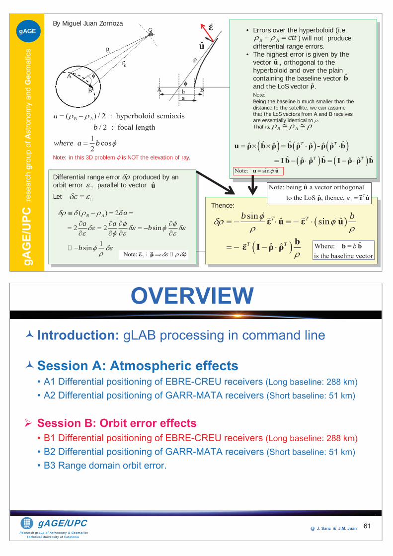
gAG
E/U
PC re
sear
ch g
roup
of A
stro
nom
y an
d G
eom
atic
sgAGE
Master of Science in GNSS J. Sanz Subirana, JM. Juan Zornoza, M. Hernández-Pajares,
• Errors over the hyperboloid (i.e. ) will not produce
differential range errors.• The highest error is given by the
vector , orthogonal to the hyperboloid and over the plain containing the baseline vector and the LoS vector .Note: Being the baseline b much smaller than the distance to the satellite, we can assume that the LoS vectors from A and B receives are essentially identical to .That is,
u
ρb
uB A ctt
( ) / 2 : hyperboloid semiaxis/ 2 : focal length
1 cos2
B Aab
where a b
B A
( ) 2
2 2 sin
1sin
B A aa a b
bsinb
ˆ ˆ ˆˆ ˆ ˆ ˆ ˆ ˆ
ˆ ˆ ˆˆ ˆ ˆ ˆ
T T
T T
u ρ b ρ b ρ ρ -ρ ρ b
Ib ρ ρ b I ρ ρ b
ε
sin ˆ ˆsin
ˆ ˆ
ˆ ˆˆ sin
ˆ ˆ
T T
T T
b bε u ε u
bε I ρ ρ
Differential range error produced by anorbit error parallel to vector Let
Thence:
Note: ε ρε ρε
ˆNote: being a vector orthogonalˆ ˆ to the LoS , thence, ˆT
uρ ε u
u
ˆWhere: is the baseline vector
bb = b
ˆNote: sin u u
By Miguel Juan Zornoza
Note: in this 3D problem is NOT the elevation of ray.
Research group of Astronomy & GeomaticsTechnical University of Catalonia
gAGE/UPC @ J. Sanz & J.M. Juan
Introduction: gLAB processing in command line
Session A: Atmospheric effects• A1 Differential positioning of EBRE-CREU receivers (Long baseline: 288 km) • A2 Differential positioning of GARR-MATA receivers (Short baseline: 51 km)
Session B: Orbit error effects• B1 Differential positioning of EBRE-CREU receivers (Long baseline: 288 km)• B2 Differential positioning of GARR-MATA receivers (Short baseline: 51 km)• B3 Range domain orbit error.
OVERVIEW
61
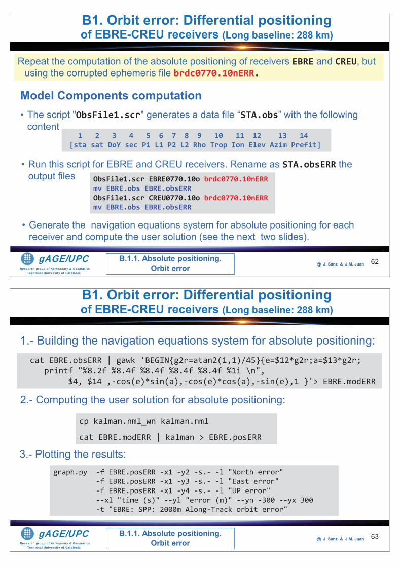
Research group of Astronomy & GeomaticsTechnical University of Catalonia
gAGE/UPC @ J. Sanz & J.M. Juan
Model Components computation• The script "ObsFile1.scr" generates a data file “STA.obs” with the following
content
62
1 2 3 4 5 6 7 8 9 10 11 12 13 14[sta sat DoY sec P1 L1 P2 L2 Rho Trop Ion Elev Azim Prefit]
• Run this script for EBRE and CREU receivers. Rename as STA.obsERR the output files ObsFile1.scr EBRE0770.10o brdc0770.10nERR
mv EBRE.obs EBRE.obsERRObsFile1.scr CREU0770.10o brdc0770.10nERRmv EBRE.obs EBRE.obsERR
• Generate the navigation equations system for absolute positioning for each receiver and compute the user solution (see the next two slides).
Repeat the computation of the absolute positioning of receivers EBRE and CREU, but using the corrupted ephemeris file brdc0770.10nERR.
B1. Orbit error: Differential positioning of EBRE-CREU receivers (Long baseline: 288 km)
B.1.1. Absolute positioning.Orbit error
Research group of Astronomy & GeomaticsTechnical University of Catalonia
gAGE/UPC @ J. Sanz & J.M. Juan
2.- Computing the user solution for absolute positioning:
63
cp kalman.nml_wn kalman.nml
cat EBRE.modERR | kalman > EBRE.posERR
3.- Plotting the results:graph.py -f EBRE.posERR -x1 -y2 -s.- -l "North error"
-f EBRE.posERR -x1 -y3 -s.- -l "East error" -f EBRE.posERR -x1 -y4 -s.- -l "UP error" --xl "time (s)" --yl "error (m)" --yn -300 --yx 300 -t "EBRE: SPP: 2000m Along-Track orbit error"
1.- Building the navigation equations system for absolute positioning: cat EBRE.obsERR | gawk 'BEGIN{g2r=atan2(1,1)/45}{e=$12*g2r;a=$13*g2r;
printf "%8.2f %8.4f %8.4f %8.4f %8.4f %1i \n",$4, $14 ,-cos(e)*sin(a),-cos(e)*cos(a),-sin(e),1 }'> EBRE.modERR
B1. Orbit error: Differential positioning of EBRE-CREU receivers (Long baseline: 288 km)
B.1.1. Absolute positioning.Orbit error
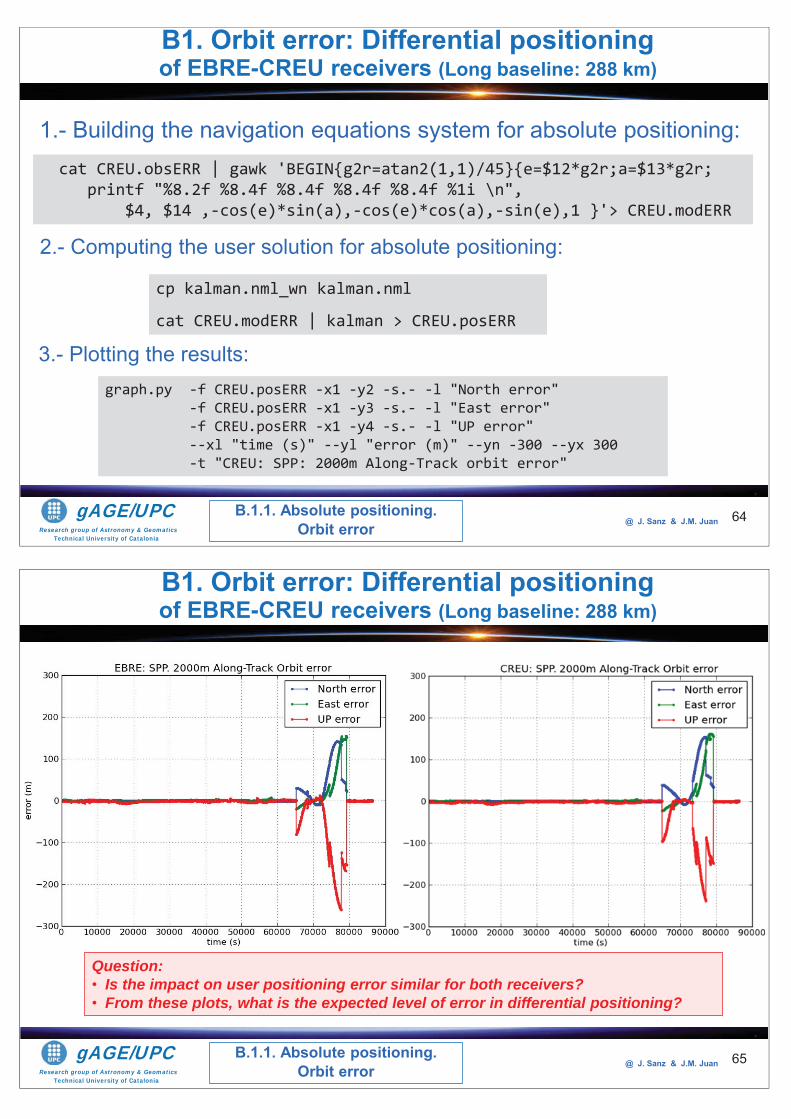
Research group of Astronomy & GeomaticsTechnical University of Catalonia
gAGE/UPC @ J. Sanz & J.M. Juan
2.- Computing the user solution for absolute positioning:
64
cp kalman.nml_wn kalman.nml
cat CREU.modERR | kalman > CREU.posERR
3.- Plotting the results:graph.py -f CREU.posERR -x1 -y2 -s.- -l "North error"
-f CREU.posERR -x1 -y3 -s.- -l "East error" -f CREU.posERR -x1 -y4 -s.- -l "UP error" --xl "time (s)" --yl "error (m)" --yn -300 --yx 300 -t "CREU: SPP: 2000m Along-Track orbit error"
1.- Building the navigation equations system for absolute positioning: cat CREU.obsERR | gawk 'BEGIN{g2r=atan2(1,1)/45}{e=$12*g2r;a=$13*g2r;
printf "%8.2f %8.4f %8.4f %8.4f %8.4f %1i \n",$4, $14 ,-cos(e)*sin(a),-cos(e)*cos(a),-sin(e),1 }'> CREU.modERR
B1. Orbit error: Differential positioning of EBRE-CREU receivers (Long baseline: 288 km)
B.1.1. Absolute positioning.Orbit error
Research group of Astronomy & GeomaticsTechnical University of Catalonia
gAGE/UPC @ J. Sanz & J.M. Juan 65
B1. Orbit error: Differential positioning of EBRE-CREU receivers (Long baseline: 288 km)
B.1.1. Absolute positioning.Orbit error
Question: • Is the impact on user positioning error similar for both receivers?• From these plots, what is the expected level of error in differential positioning?
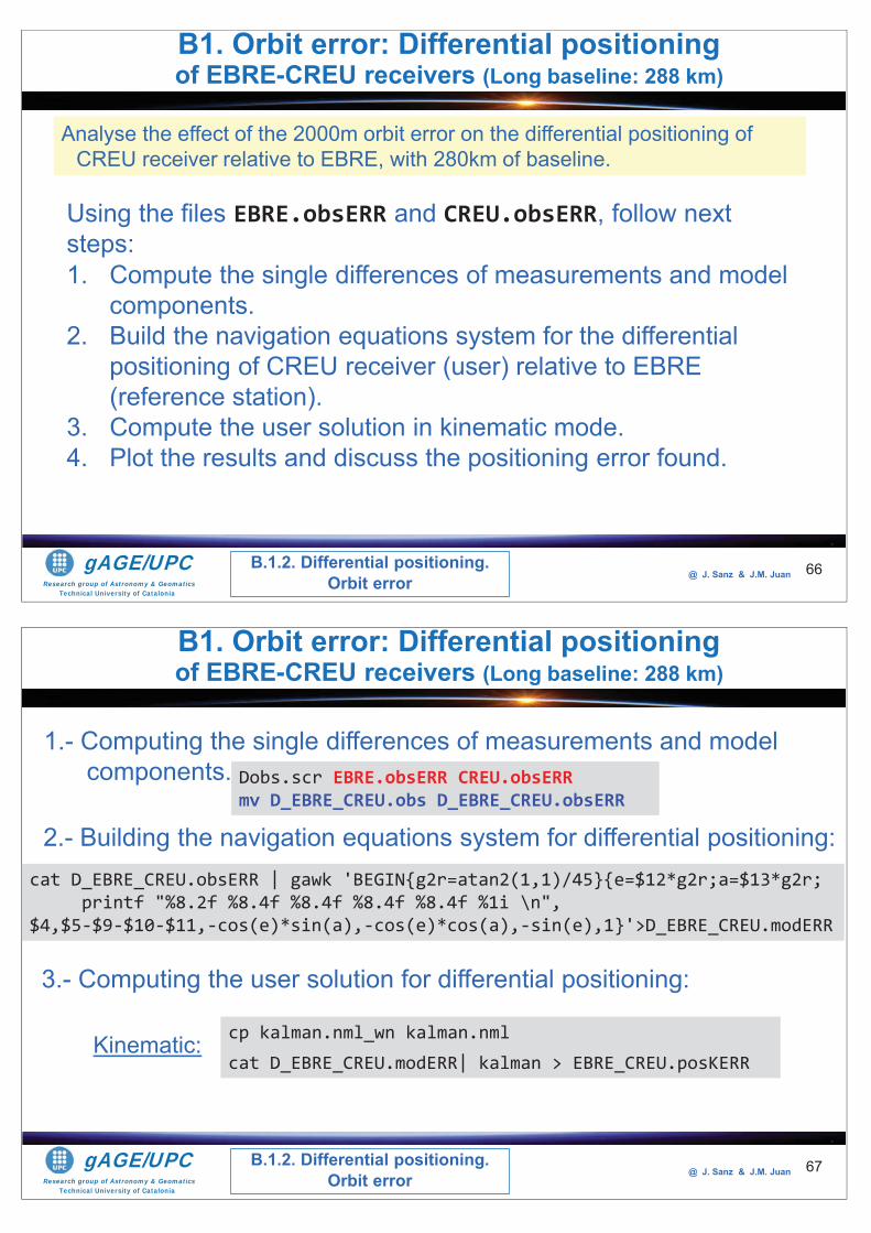
Research group of Astronomy & GeomaticsTechnical University of Catalonia
gAGE/UPC @ J. Sanz & J.M. Juan 66
Using the files EBRE.obsERR and CREU.obsERR, follow next steps:1. Compute the single differences of measurements and model
components.2. Build the navigation equations system for the differential
positioning of CREU receiver (user) relative to EBRE (reference station).
3. Compute the user solution in kinematic mode.4. Plot the results and discuss the positioning error found.
Analyse the effect of the 2000m orbit error on the differential positioning of CREU receiver relative to EBRE, with 280km of baseline.
B1. Orbit error: Differential positioning of EBRE-CREU receivers (Long baseline: 288 km)
B.1.2. Differential positioning.Orbit error
Research group of Astronomy & GeomaticsTechnical University of Catalonia
gAGE/UPC @ J. Sanz & J.M. Juan
3.- Computing the user solution for differential positioning:
67
cp kalman.nml_wn kalman.nmlcat D_EBRE_CREU.modERR| kalman > EBRE_CREU.posKERR
2.- Building the navigation equations system for differential positioning: cat D_EBRE_CREU.obsERR | gawk 'BEGIN{g2r=atan2(1,1)/45}{e=$12*g2r;a=$13*g2r;
printf "%8.2f %8.4f %8.4f %8.4f %8.4f %1i \n",$4,$5-$9-$10-$11,-cos(e)*sin(a),-cos(e)*cos(a),-sin(e),1}'>D_EBRE_CREU.modERR
1.- Computing the single differences of measurements and model components. Dobs.scr EBRE.obsERR CREU.obsERR
mv D_EBRE_CREU.obs D_EBRE_CREU.obsERR
Kinematic:
B1. Orbit error: Differential positioning of EBRE-CREU receivers (Long baseline: 288 km)
B.1.2. Differential positioning.Orbit error
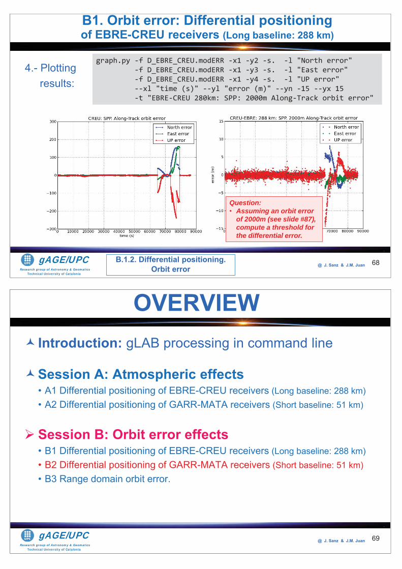
Research group of Astronomy & GeomaticsTechnical University of Catalonia
gAGE/UPC @ J. Sanz & J.M. Juan 68
4.- Plotting results:
graph.py -f D_EBRE_CREU.modERR -x1 -y2 -s. -l "North error" -f D_EBRE_CREU.modERR -x1 -y3 -s. -l "East error" -f D_EBRE_CREU.modERR -x1 -y4 -s. -l "UP error" --xl "time (s)" --yl "error (m)" --yn -15 --yx 15 -t "EBRE-CREU 280km: SPP: 2000m Along-Track orbit error"
B1. Orbit error: Differential positioning of EBRE-CREU receivers (Long baseline: 288 km)
B.1.2. Differential positioning.Orbit error
Question: • Assuming an orbit error
of 2000m (see slide #87), compute a threshold for the differential error.
Research group of Astronomy & GeomaticsTechnical University of Catalonia
gAGE/UPC @ J. Sanz & J.M. Juan
Introduction: gLAB processing in command line
Session A: Atmospheric effects• A1 Differential positioning of EBRE-CREU receivers (Long baseline: 288 km) • A2 Differential positioning of GARR-MATA receivers (Short baseline: 51 km)
Session B: Orbit error effects• B1 Differential positioning of EBRE-CREU receivers (Long baseline: 288 km) • B2 Differential positioning of GARR-MATA receivers (Short baseline: 51 km)• B3 Range domain orbit error.
OVERVIEW
69

Research group of Astronomy & GeomaticsTechnical University of Catalonia
gAGE/UPC @ J. Sanz & J.M. Juan
Model Components computation• The script "ObsFile1.scr" generates a data file “STA.obs” with the following
content
70
1 2 3 4 5 6 7 8 9 10 11 12 13 14[sta sat DoY sec P1 L1 P2 L2 Rho Trop Ion Elev Azim Prefit]
• Run this script for GARR and MATA receivers. Rename as STA.obsERR the output files ObsFile1.scr GARR0770.10o brdc0770.10nERR
mv GARR.obs GARR.obsERRObsFile1.scr MATA0770.10o brdc0770.10nERRmv MATA.obs MATA.obsERR
• Generate the navigation equations system for absolute positioning for each receiver and compute the user solution (see next two slides).
Repeat the computation of the absolute positioning of receivers GARR and MATA, but using the corrupted ephemeris file brdc0770.10nERR.
B2. Orbit error: Differential positioning of GARR-MATA receivers (Short baseline: 51 km)
B.2.1. Absolute positioning.Orbit error
Research group of Astronomy & GeomaticsTechnical University of Catalonia
gAGE/UPC @ J. Sanz & J.M. Juan
2.- Computing the user solution for absolute positioning:
71
cp kalman.nml_wn kalman.nml
cat GARR.modERR | kalman > GARR.posERR
3.- Plotting the results:graph.py -f GARR.posERR -x1 -y2 -s.- -l "North error"
-f GARR.posERR -x1 -y3 -s.- -l "East error" -f GARR.posERR -x1 -y4 -s.- -l "UP error" --xl "time (s)" --yl "error (m)" --yn -300 --yx 300 -t "GARR: SPP: 2000m Along-Track orbit error"
1.- Building the navigation equations system for absolute positioning: cat GARR.obsERR | gawk 'BEGIN{g2r=atan2(1,1)/45}{e=$12*g2r;a=$13*g2r;
printf "%8.2f %8.4f %8.4f %8.4f %8.4f %1i \n",$4, $14 ,-cos(e)*sin(a),-cos(e)*cos(a),-sin(e),1 }'> GARR.modERR
B2. Orbit error: Differential positioning of GARR-MATA receivers (Short baseline: 51 km)
B.2.1. Absolute positioning.Orbit error
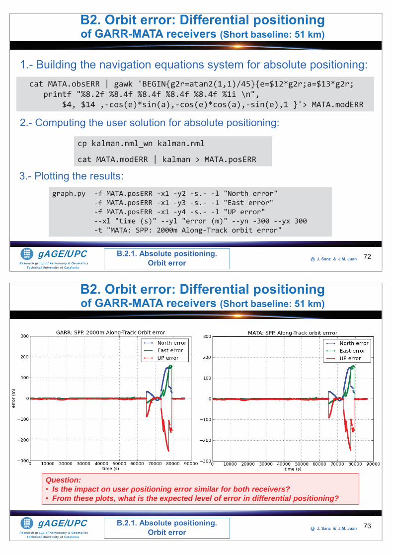
Research group of Astronomy & GeomaticsTechnical University of Catalonia
gAGE/UPC @ J. Sanz & J.M. Juan
2.- Computing the user solution for absolute positioning:
72
cp kalman.nml_wn kalman.nml
cat MATA.modERR | kalman > MATA.posERR
3.- Plotting the results:graph.py -f MATA.posERR -x1 -y2 -s.- -l "North error"
-f MATA.posERR -x1 -y3 -s.- -l "East error" -f MATA.posERR -x1 -y4 -s.- -l "UP error" --xl "time (s)" --yl "error (m)" --yn -300 --yx 300 -t "MATA: SPP: 2000m Along-Track orbit error"
1.- Building the navigation equations system for absolute positioning: cat MATA.obsERR | gawk 'BEGIN{g2r=atan2(1,1)/45}{e=$12*g2r;a=$13*g2r;
printf "%8.2f %8.4f %8.4f %8.4f %8.4f %1i \n",$4, $14 ,-cos(e)*sin(a),-cos(e)*cos(a),-sin(e),1 }'> MATA.modERR
B2. Orbit error: Differential positioning of GARR-MATA receivers (Short baseline: 51 km)
B.2.1. Absolute positioning.Orbit error
Research group of Astronomy & GeomaticsTechnical University of Catalonia
gAGE/UPC @ J. Sanz & J.M. Juan 73
B2. Orbit error: Differential positioning of GARR-MATA receivers (Short baseline: 51 km)
B.2.1. Absolute positioning.Orbit error
Question: • Is the impact on user positioning error similar for both receivers?• From these plots, what is the expected level of error in differential positioning?
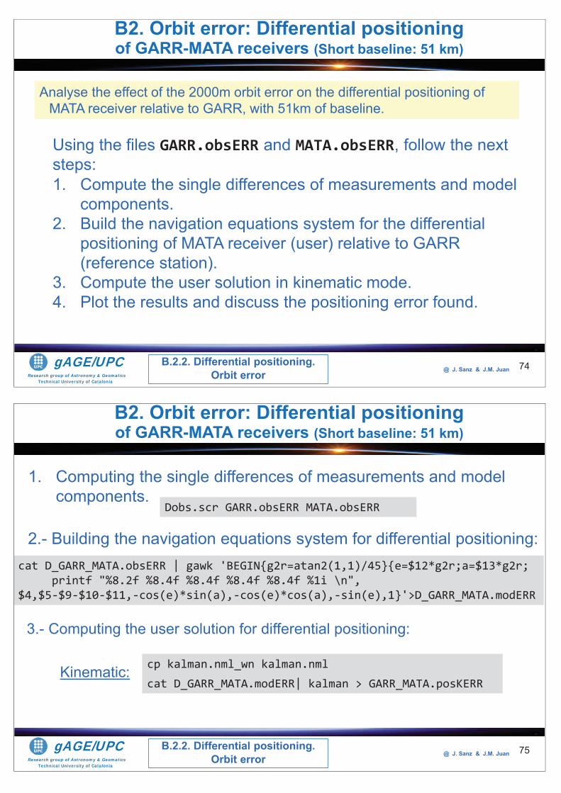
Research group of Astronomy & GeomaticsTechnical University of Catalonia
gAGE/UPC @ J. Sanz & J.M. Juan 74
Using the files GARR.obsERR and MATA.obsERR, follow the next steps:1. Compute the single differences of measurements and model
components.2. Build the navigation equations system for the differential
positioning of MATA receiver (user) relative to GARR (reference station).
3. Compute the user solution in kinematic mode.4. Plot the results and discuss the positioning error found.
Analyse the effect of the 2000m orbit error on the differential positioning of MATA receiver relative to GARR, with 51km of baseline.
B.2.2. Differential positioning.Orbit error
B2. Orbit error: Differential positioning of GARR-MATA receivers (Short baseline: 51 km)
Research group of Astronomy & GeomaticsTechnical University of Catalonia
gAGE/UPC @ J. Sanz & J.M. Juan
3.- Computing the user solution for differential positioning:
75
cp kalman.nml_wn kalman.nmlcat D_GARR_MATA.modERR| kalman > GARR_MATA.posKERR
2.- Building the navigation equations system for differential positioning: cat D_GARR_MATA.obsERR | gawk 'BEGIN{g2r=atan2(1,1)/45}{e=$12*g2r;a=$13*g2r;
printf "%8.2f %8.4f %8.4f %8.4f %8.4f %1i \n",$4,$5-$9-$10-$11,-cos(e)*sin(a),-cos(e)*cos(a),-sin(e),1}'>D_GARR_MATA.modERR
1. Computing the single differences of measurements and model components.
Dobs.scr GARR.obsERR MATA.obsERR
Kinematic:
B.2.2. Differential positioning.Orbit error
B2. Orbit error: Differential positioning of GARR-MATA receivers (Short baseline: 51 km)
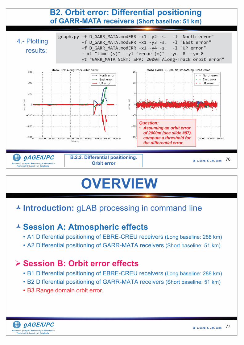
Research group of Astronomy & GeomaticsTechnical University of Catalonia
gAGE/UPC @ J. Sanz & J.M. Juan 76
4.- Plotting results:
graph.py -f D_GARR_MATA.modERR -x1 -y2 -s. -l "North error" -f D_GARR_MATA.modERR -x1 -y3 -s. -l "East error" -f D_GARR_MATA.modERR -x1 -y4 -s. -l "UP error" --xl "time (s)" --yl "error (m)" --yn -8 --yx 8 -t "GARR_MATA 51km: SPP: 2000m Along-Track orbit error"
B.2.2. Differential positioning.Orbit error
B2. Orbit error: Differential positioning of GARR-MATA receivers (Short baseline: 51 km)
Question: • Assuming an orbit error
of 2000m (see slide #87), compute a threshold for the differential error.
Research group of Astronomy & GeomaticsTechnical University of Catalonia
gAGE/UPC @ J. Sanz & J.M. Juan
Introduction: gLAB processing in command line
Session A: Atmospheric effects• A1 Differential positioning of EBRE-CREU receivers (Long baseline: 288 km) • A2 Differential positioning of GARR-MATA receivers (Short baseline: 51 km)
Session B: Orbit error effects• B1 Differential positioning of EBRE-CREU receivers (Long baseline: 288 km) • B2 Differential positioning of GARR-MATA receivers (Short baseline: 51 km)• B3 Range domain orbit error.
OVERVIEW
77
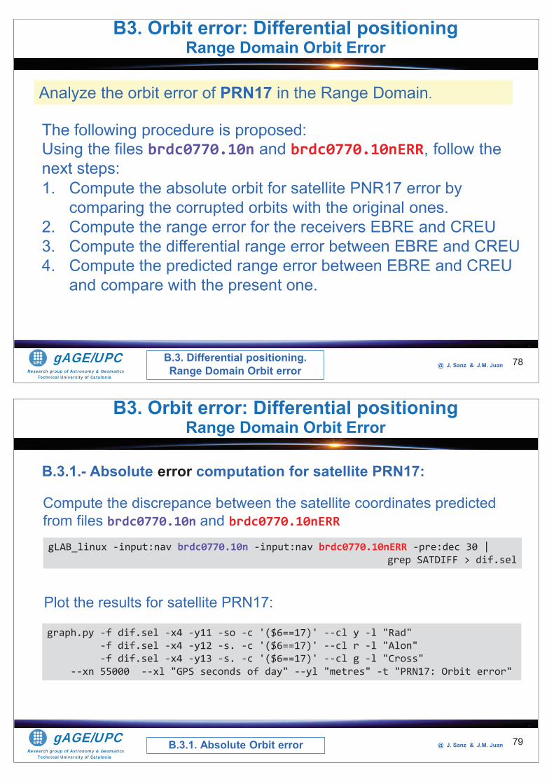
Research group of Astronomy & GeomaticsTechnical University of Catalonia
gAGE/UPC @ J. Sanz & J.M. Juan 78
The following procedure is proposed:Using the files brdc0770.10n and brdc0770.10nERR, follow the next steps:1. Compute the absolute orbit for satellite PNR17 error by
comparing the corrupted orbits with the original ones.2. Compute the range error for the receivers EBRE and CREU3. Compute the differential range error between EBRE and CREU4. Compute the predicted range error between EBRE and CREU
and compare with the present one.
Analyze the orbit error of PRN17 in the Range Domain.
B.3. Differential positioning.Range Domain Orbit error
B3. Orbit error: Differential positioning Range Domain Orbit Error
Research group of Astronomy & GeomaticsTechnical University of Catalonia
gAGE/UPC @ J. Sanz & J.M. Juan 79
B.3.1.- Absolute error computation for satellite PRN17:
gLAB_linux -input:nav brdc0770.10n -input:nav brdc0770.10nERR -pre:dec 30 |grep SATDIFF > dif.sel
B.3.1. Absolute Orbit error
B3. Orbit error: Differential positioning Range Domain Orbit Error
graph.py -f dif.sel -x4 -y11 -so -c '($6==17)' --cl y -l "Rad" -f dif.sel -x4 -y12 -s. -c '($6==17)' --cl r -l "Alon" -f dif.sel -x4 -y13 -s. -c '($6==17)' --cl g -l "Cross"
--xn 55000 --xl "GPS seconds of day" --yl "metres" -t "PRN17: Orbit error"
Compute the discrepance between the satellite coordinates predicted from files brdc0770.10n and brdc0770.10nERR
Plot the results for satellite PRN17:
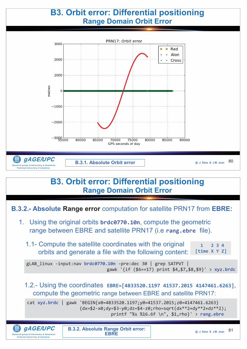
Research group of Astronomy & GeomaticsTechnical University of Catalonia
gAGE/UPC @ J. Sanz & J.M. Juan 80B.3.1. Absolute Orbit error
B3. Orbit error: Differential positioning Range Domain Orbit Error
Research group of Astronomy & GeomaticsTechnical University of Catalonia
gAGE/UPC @ J. Sanz & J.M. Juan 81
B.3.2.- Absolute Range error computation for satellite PRN17 from EBRE:
gLAB_linux -input:nav brdc0770.10n -pre:dec 30 | grep SATPVT | gawk '{if ($6==17) print $4,$7,$8,$9}' > xyz.brdc
B.3.2. Absolute Range Orbit error: EBRE
B3. Orbit error: Differential positioning Range Domain Orbit Error
1. Using the original orbits brdc0770.10n, compute the geometric range between EBRE and satellite PRN17 (i.e rang.ebre file).
1.1- Compute the satellite coordinates with the original orbits and generate a file with the following content:
1 2 3 4[time X Y Z]
cat xyz.brdc | gawk 'BEGIN{x0=4833520.1197;y0=41537.2015;z0=4147461.6263}{dx=$2-x0;dy=$3-y0;dz=$4-z0;rho=sqrt(dx**2+dy**2+dz**2);
printf "%s %16.6f \n", $1,rho}' > rang.ebre
1.2.- Using the coordinates EBRE=[4833520.1197 41537.2015 4147461.6263], compute the geometric range between EBRE and satellite PRN17:
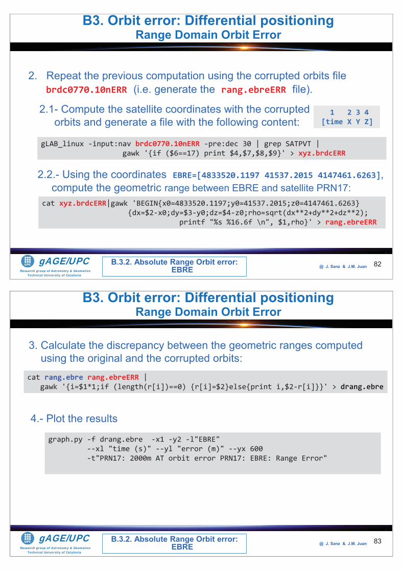
Research group of Astronomy & GeomaticsTechnical University of Catalonia
gAGE/UPC @ J. Sanz & J.M. Juan 82
gLAB_linux -input:nav brdc0770.10nERR -pre:dec 30 | grep SATPVT |gawk '{if ($6==17) print $4,$7,$8,$9}' > xyz.brdcERR
B3. Orbit error: Differential positioning Range Domain Orbit Error
2. Repeat the previous computation using the corrupted orbits file brdc0770.10nERR (i.e. generate the rang.ebreERR file).
2.1- Compute the satellite coordinates with the corrupted orbits and generate a file with the following content:
1 2 3 4[time X Y Z]
cat xyz.brdcERR|gawk 'BEGIN{x0=4833520.1197;y0=41537.2015;z0=4147461.6263}{dx=$2-x0;dy=$3-y0;dz=$4-z0;rho=sqrt(dx**2+dy**2+dz**2);
printf "%s %16.6f \n", $1,rho}' > rang.ebreERR
2.2.- Using the coordinates EBRE=[4833520.1197 41537.2015 4147461.6263], compute the geometric range between EBRE and satellite PRN17:
B.3.2. Absolute Range Orbit error: EBRE
Research group of Astronomy & GeomaticsTechnical University of Catalonia
gAGE/UPC @ J. Sanz & J.M. Juan 83
cat rang.ebre rang.ebreERR | gawk '{i=$1*1;if (length(r[i])==0) {r[i]=$2}else{print i,$2-r[i]}}' > drang.ebre
B3. Orbit error: Differential positioning Range Domain Orbit Error
3. Calculate the discrepancy between the geometric ranges computed using the original and the corrupted orbits:
graph.py -f drang.ebre -x1 -y2 -l"EBRE" --xl "time (s)" --yl "error (m)" --yx 600 -t"PRN17: 2000m AT orbit error PRN17: EBRE: Range Error"
4.- Plot the results
B.3.2. Absolute Range Orbit error: EBRE
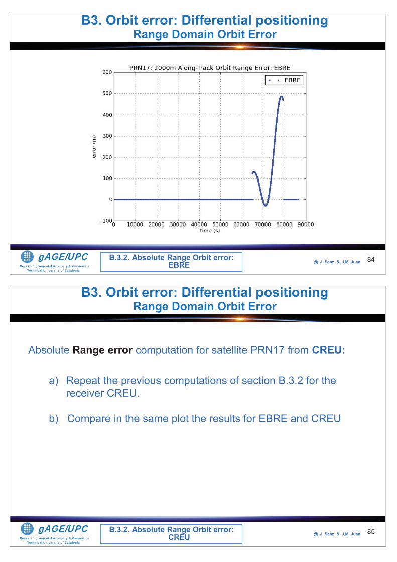
Research group of Astronomy & GeomaticsTechnical University of Catalonia
gAGE/UPC @ J. Sanz & J.M. Juan 84
B3. Orbit error: Differential positioning Range Domain Orbit Error
B.3.2. Absolute Range Orbit error: EBRE
Research group of Astronomy & GeomaticsTechnical University of Catalonia
gAGE/UPC @ J. Sanz & J.M. Juan 85
Absolute Range error computation for satellite PRN17 from CREU:
a) Repeat the previous computations of section B.3.2 for the receiver CREU.
b) Compare in the same plot the results for EBRE and CREU
B.3.2. Absolute Range Orbit error: CREU
B3. Orbit error: Differential positioning Range Domain Orbit Error
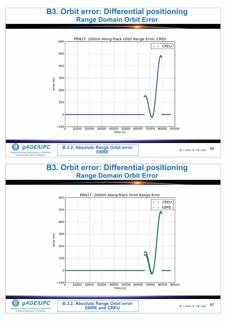
Research group of Astronomy & GeomaticsTechnical University of Catalonia
gAGE/UPC @ J. Sanz & J.M. Juan 86
B3. Orbit error: Differential positioning Range Domain Orbit Error
B.3.2. Absolute Range Orbit error: EBRE
Research group of Astronomy & GeomaticsTechnical University of Catalonia
gAGE/UPC @ J. Sanz & J.M. Juan 87
B3. Orbit error: Differential positioning Range Domain Orbit Error
B.3.2. Absolute Range Orbit error: EBRE and CREU
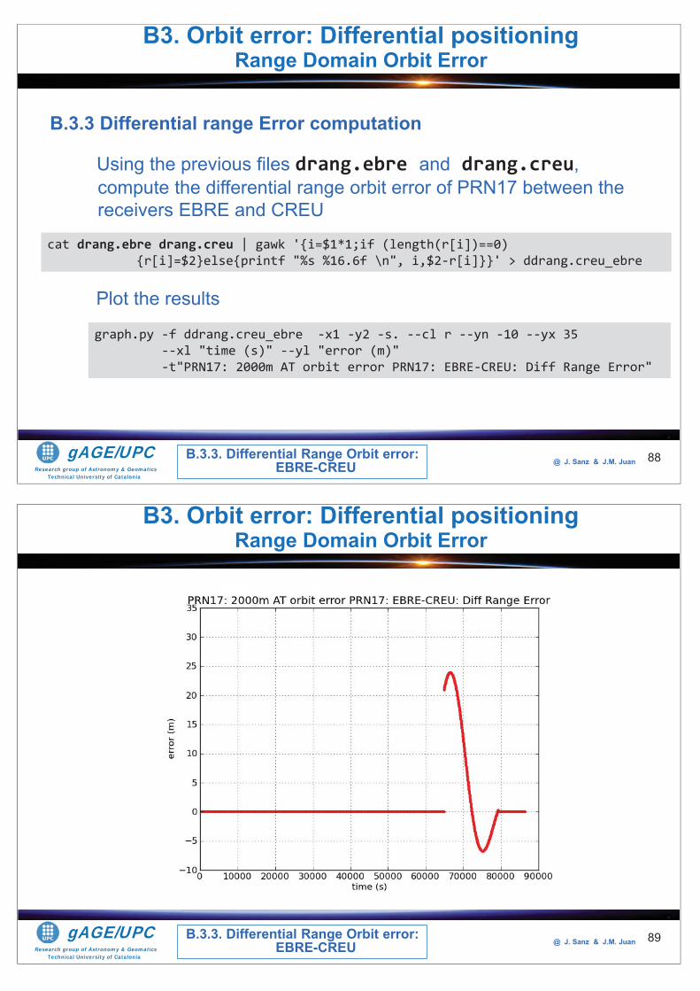
Research group of Astronomy & GeomaticsTechnical University of Catalonia
gAGE/UPC @ J. Sanz & J.M. Juan 88
B3. Orbit error: Differential positioning Range Domain Orbit Error
B.3.3. Differential Range Orbit error: EBRE-CREU
B.3.3 Differential range Error computation
Using the previous files drang.ebre and drang.creu, compute the differential range orbit error of PRN17 between the receivers EBRE and CREU
cat drang.ebre drang.creu | gawk '{i=$1*1;if (length(r[i])==0) {r[i]=$2}else{printf "%s %16.6f \n", i,$2-r[i]}}' > ddrang.creu_ebre
graph.py -f ddrang.creu_ebre -x1 -y2 -s. --cl r --yn -10 --yx 35 --xl "time (s)" --yl "error (m)" -t"PRN17: 2000m AT orbit error PRN17: EBRE-CREU: Diff Range Error"
Plot the results
Research group of Astronomy & GeomaticsTechnical University of Catalonia
gAGE/UPC @ J. Sanz & J.M. Juan 89
B3. Orbit error: Differential positioning Range Domain Orbit Error
B.3.3. Differential Range Orbit error: EBRE-CREU
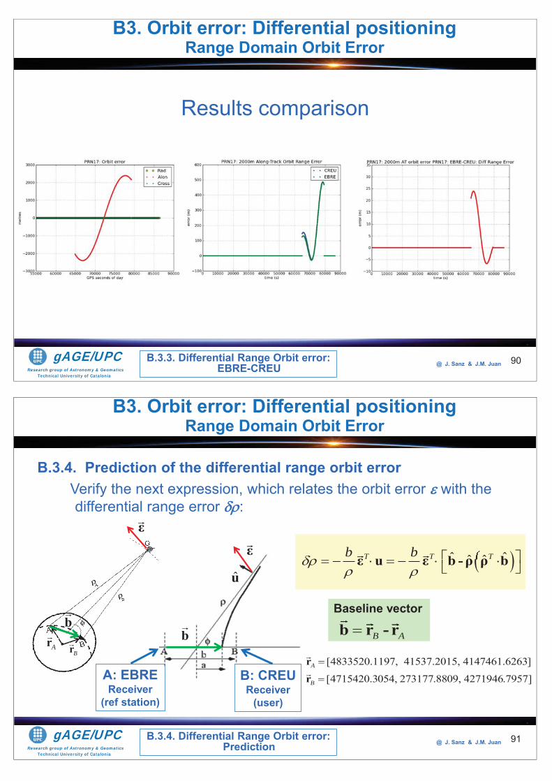
Research group of Astronomy & GeomaticsTechnical University of Catalonia
gAGE/UPC @ J. Sanz & J.M. Juan 90
B3. Orbit error: Differential positioning Range Domain Orbit Error
B.3.3. Differential Range Orbit error: EBRE-CREU
Results comparison
Research group of Astronomy & GeomaticsTechnical University of Catalonia
gAGE/UPC @ J. Sanz & J.M. Juan 91
u
ε
B.3.4. Prediction of the differential range orbit errorVerify the next expression, which relates the orbit error with the differential range error :
B3. Orbit error: Differential positioning Range Domain Orbit Error
B.3.4. Differential Range Orbit error: Prediction
ˆ ˆˆ ˆˆ ˆ ˆT T Tb bε u ε b -ρ ρ b
B: CREUReceiver
(user)
A: EBREReceiver
(ref station)
b B Ab r - rBaseline vector
[4833520.1197, 41537.2015, 4147461.6263][4833Ar[4715420.3054, 273177.8809, 4271946.7957][4715Br
ArBr
ε
b
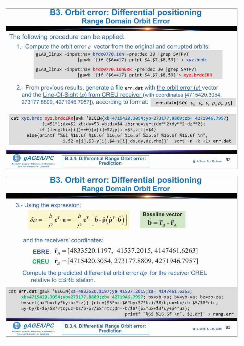
Research group of Astronomy & GeomaticsTechnical University of Catalonia
gAGE/UPC @ J. Sanz & J.M. Juan 92
The following procedure can be applied:
B3. Orbit error: Differential positioning Range Domain Orbit Error
1.- Compute the orbit error vector from the original and corrupted orbits:gLAB_linux -input:nav brdc0770.10n -pre:dec 30 |grep SATPVT
|gawk '{if ($6==17) print $4,$7,$8,$9}' > xyz.brdc
gLAB_linux -input:nav brdc0770.10nERR -pre:dec 30 |grep SATPVT |gawk '{if ($6==17) print $4,$7,$8,$9}'> xyz.brdcERR
2.- From previous results, generate a file err.dat with the orbit error ( ) vector and the Line-Of-Sight ( ) from CREU receiver (with coordinates [4715420.3054, 273177.8809, 4271946.7957]), according to format:
cat xyz.brdc xyz.brdcERR|awk 'BEGIN{xb=4715420.3054;yb=273177.8809;zb= 4271946.7957} {i=$1*1;dx=$2-xb;dy=$3-yb;dz=$4-zb;rho=sqrt(dx**2+dy**2+dz**2); if (length(x[i])==0){x[i]=$2;y[i]=$3;z[i]=$4}
else{printf "%6i %16.6f %16.6f %16.6f %16.6f %16.6f %16.6f %16.6f \n", i,$2-x[i],$3-y[i],$4-z[i],dx,dy,dz,rho}}' |sort -n -k +1> err.dat
err.dat=[sec x y z x y z]
B.3.4. Differential Range Orbit error: Prediction
Research group of Astronomy & GeomaticsTechnical University of Catalonia
gAGE/UPC @ J. Sanz & J.M. Juan 93
3.- Using the expression:
B3. Orbit error: Differential positioning Range Domain Orbit Error
B.3.4. Differential Range Orbit error: Prediction
and the receivers’ coordinates:
ˆ ˆˆ ˆˆ ˆ ˆT T Tb bε u ε b -ρ ρ bB Ab r - r
Baseline vector
[4833520.1197, 41537.2015, 4147461.6263][4833Ar[4715420.3054, 273177.8809, 4271946.7957][4715Br
Compute the predicted differential orbit error d for the receiver CREU relative to EBRE station.
CREU:EBRE:
cat err.dat|gawk 'BEGIN{xa=4833520.1197;ya=41537.2015;za= 4147461.6263; xb=4715420.3054;yb=273177.8809;zb= 4271946.7957; bx=xb-xa; by=yb-ya; bz=zb-za; b=sqrt(bx*bx+by*by+bz*cz)} {rtc=($5*bx+$6*by+$7*bz)/$8/b;ux=bx/cb-$5/$8*rtc; uy=by/b-$6/$8*rtc;uz=bz/b-$7/$8*rtc;dr=-b/$8*($2*ux+$3*uy+$4*uz);
printf "%6i %16.6f \n", $1,dr}' > rang.err
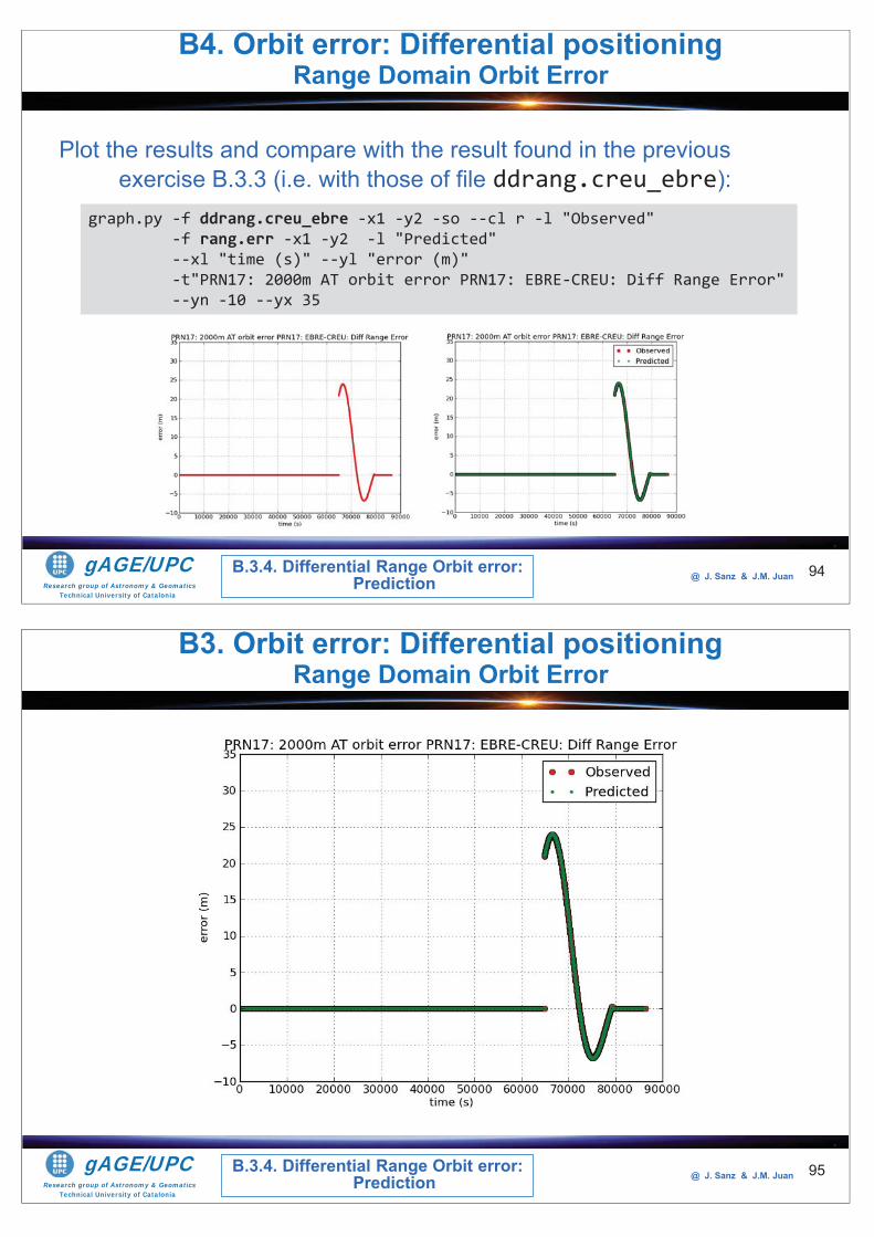
Research group of Astronomy & GeomaticsTechnical University of Catalonia
gAGE/UPC @ J. Sanz & J.M. Juan 94
Plot the results and compare with the result found in the previous exercise B.3.3 (i.e. with those of file ddrang.creu_ebre):
B4. Orbit error: Differential positioning Range Domain Orbit Error
B.3.4. Differential Range Orbit error: Prediction
graph.py -f ddrang.creu_ebre -x1 -y2 -so --cl r -l "Observed" -f rang.err -x1 -y2 -l "Predicted" --xl "time (s)" --yl "error (m)" -t"PRN17: 2000m AT orbit error PRN17: EBRE-CREU: Diff Range Error" --yn -10 --yx 35
Research group of Astronomy & GeomaticsTechnical University of Catalonia
gAGE/UPC @ J. Sanz & J.M. Juan 95
B3. Orbit error: Differential positioning Range Domain Orbit Error
B.3.4. Differential Range Orbit error: Prediction
Research group of Astronomy & GeomaticsTechnical University of Catalonia
gAGE/UPC @ J. Sanz & J.M. Juan 96
Thanks for yourattention
Research group of Astronomy & GeomaticsTechnical University of Catalonia
gAGE/UPC @ J. Sanz & J.M. Juan
• To Institut Cartografic de Catalunya for the data files of receivers EBRE, CREU, GARR and MATA.
• To Adrià Rovira-Garcia for his contribution to the editing of this material and gLAB updating and integrating this learning material into the GLUE.
The ESA/UPC GNSS-Lab Tool suite (gLAB) has been developed under the ESA Education Office contract N. P1081434.
Acknowledgements
Research group of Astronomy & GeomaticsTechnical University of Catalonia
gAGE/UPC @ J. Sanz & J.M. Juan 1
Tutorial 4Carrier ambiguity fixing
Contact: [email protected] site: http://www.gage.upc.edu
Slides associated to gLAB version 2.0.0
Research group of Astronomy & GeomaticsTechnical University of Catalonia
gAGE/UPC @ J. Sanz & J.M. Juan 3
This tutorial is devoted to analyse and assess the ambiguity fixing and the differential positioning with carrier phase measurements (L1, L2). Two receivers UPC1 and UPC2 with a baseline of about 40 metres are considered.
This study includes ambiguity fixing using the “cascade method” (i.e., fixing one at a time) and with the LAMBDA method.
The effect of synchronization errors between the reference station and the user is and its effect on the navigation and ambiguity fixing is also analysed
All software tools (including gLAB) and associated files for the laboratory session are included in the CD-ROM or USB stick associated with this tutorial.
Aim of this tutorial
Research group of Astronomy & GeomaticsTechnical University of Catalonia
gAGE/UPC @ J. Sanz & J.M. Juan
Introduction: gLAB processing in command line.
Preliminary computations: Data files.
Session A: Fixing DD ambiguities one at a time: UPC1-UPC2.
Session B: Assessing the fixed ambiguities in navigation: Differential positioning of UPC1-UPC2 receivers.
Session C: Fixing DD ambiguities with LAMBDA method.
Note: UPC1-UPC2 receivers baseline: 37.95 metres.
OVERVIEW
4
Research group of Astronomy & GeomaticsTechnical University of Catalonia
gAGE/UPC @ J. Sanz & J.M. Juan
Introduction: gLAB processing in command line.Preliminary computations: Data files.
Session A: Fixing DD ambiguities one at a time: UPC1-UPC2.
Session B: Assessing the fixed ambiguities in navigation: Differential positioning of UPC1-UPC2 receivers.
Session C: Fixing DD ambiguities with LAMBDA method.
Note: UPC1-UPC2 receivers baseline: 37.95 metres.
OVERVIEW
5
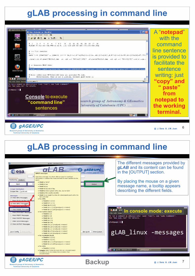
Research group of Astronomy & GeomaticsTechnical University of Catalonia
gAGE/UPC @ J. Sanz & J.M. Juan 6
Console to execute “command line”
sentences
A “notepad” with the
command line sentence is provided to facilitate the
sentence writing: just “copy” and
“ paste” from
notepad to the working
terminal.
gLAB processing in command line
Research group of Astronomy & GeomaticsTechnical University of Catalonia
gAGE/UPC @ J. Sanz & J.M. Juan 7
The different messages provided by gLAB and its content can be found in the [OUTPUT] section.
By placing the mouse on a given message name, a tooltip appears describing the different fields.
Backup
gLAB_linux -messages
In console mode: execute
gLAB processing in command line
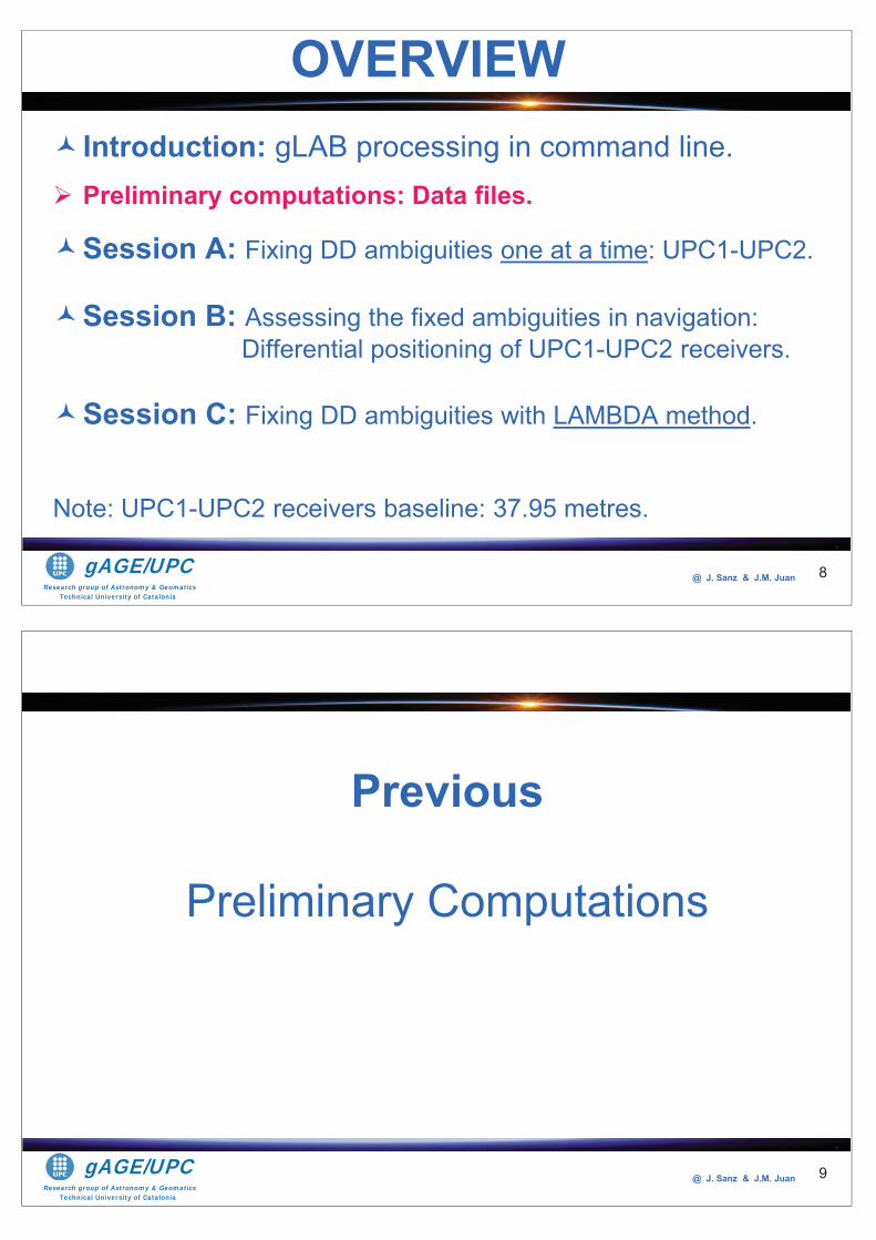
Research group of Astronomy & GeomaticsTechnical University of Catalonia
gAGE/UPC @ J. Sanz & J.M. Juan
Introduction: gLAB processing in command line.Preliminary computations: Data files.
Session A: Fixing DD ambiguities one at a time: UPC1-UPC2.
Session B: Assessing the fixed ambiguities in navigation: Differential positioning of UPC1-UPC2 receivers.
Session C: Fixing DD ambiguities with LAMBDA method.
Note: UPC1-UPC2 receivers baseline: 37.95 metres.
OVERVIEW
8
Research group of Astronomy & GeomaticsTechnical University of Catalonia
gAGE/UPC @ J. Sanz & J.M. Juan 9
Previous
Preliminary Computations
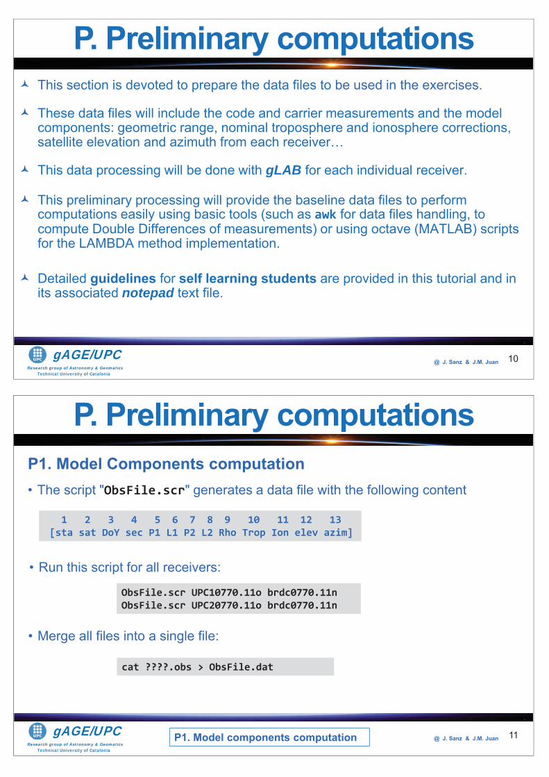
Research group of Astronomy & GeomaticsTechnical University of Catalonia
gAGE/UPC @ J. Sanz & J.M. Juan 10
This section is devoted to prepare the data files to be used in the exercises.
These data files will include the code and carrier measurements and the model components: geometric range, nominal troposphere and ionosphere corrections, satellite elevation and azimuth from each receiver…
This data processing will be done with gLAB for each individual receiver.
This preliminary processing will provide the baseline data files to perform computations easily using basic tools (such as awk for data files handling, to compute Double Differences of measurements) or using octave (MATLAB) scripts for the LAMBDA method implementation.
Detailed guidelines for self learning students are provided in this tutorial and in its associated notepad text file.
P. Preliminary computations
Research group of Astronomy & GeomaticsTechnical University of Catalonia
gAGE/UPC @ J. Sanz & J.M. Juan
P1. Model Components computation• The script "ObsFile.scr" generates a data file with the following content
11
P. Preliminary computations
1 2 3 4 5 6 7 8 9 10 11 12 13[sta sat DoY sec P1 L1 P2 L2 Rho Trop Ion elev azim]
• Run this script for all receivers:
ObsFile.scr UPC10770.11o brdc0770.11nObsFile.scr UPC20770.11o brdc0770.11n
• Merge all files into a single file:
cat ????.obs > ObsFile.dat
P1. Model components computation
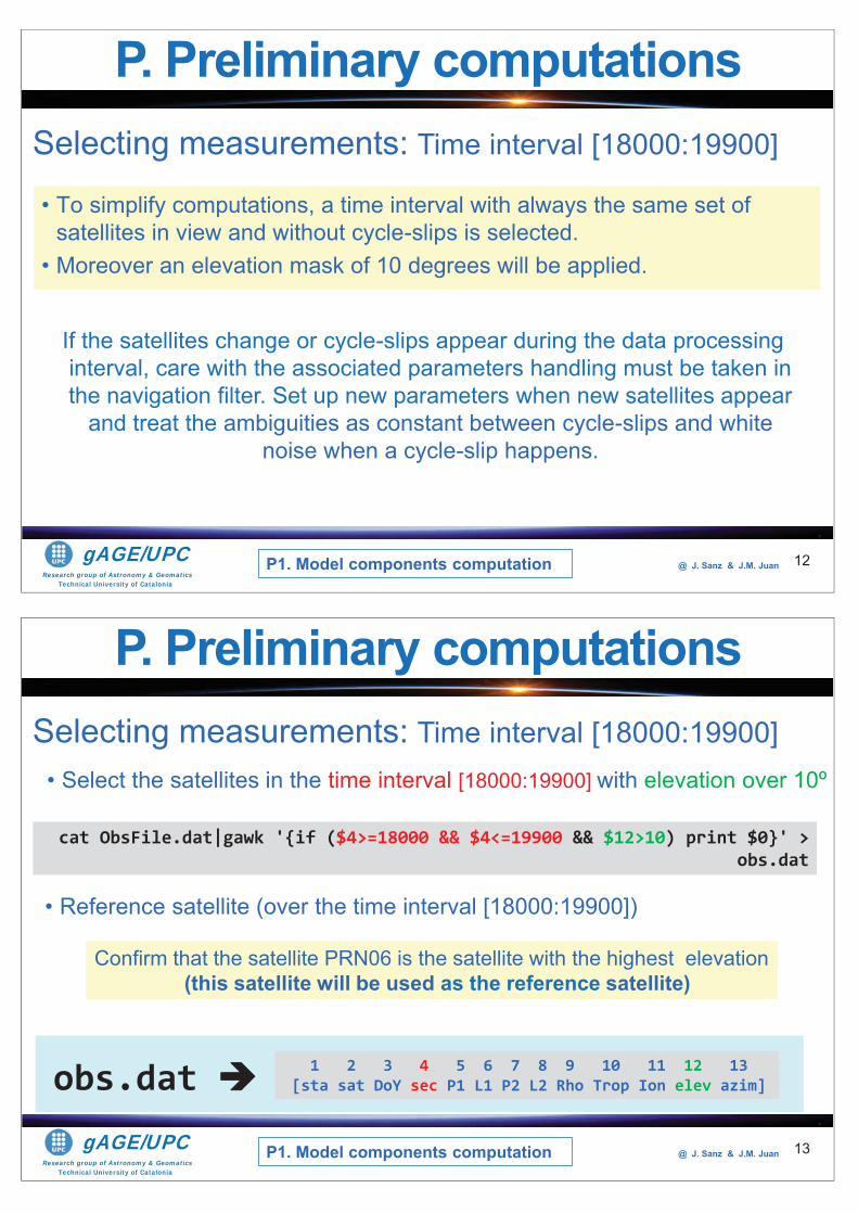
Research group of Astronomy & GeomaticsTechnical University of Catalonia
gAGE/UPC @ J. Sanz & J.M. Juan
• To simplify computations, a time interval with always the same set of satellites in view and without cycle-slips is selected.
• Moreover an elevation mask of 10 degrees will be applied.
12
P. Preliminary computationsSelecting measurements: Time interval [18000:19900]
If the satellites change or cycle-slips appear during the data processing interval, care with the associated parameters handling must be taken in the navigation filter. Set up new parameters when new satellites appear
and treat the ambiguities as constant between cycle-slips and white noise when a cycle-slip happens.
P1. Model components computation
Research group of Astronomy & GeomaticsTechnical University of Catalonia
gAGE/UPC @ J. Sanz & J.M. Juan
• Select the satellites in the time interval [18000:19900] with elevation over 10º
13
P. Preliminary computations
Confirm that the satellite PRN06 is the satellite with the highest elevation (this satellite will be used as the reference satellite)
cat ObsFile.dat|gawk '{if ($4>=18000 && $4<=19900 && $12>10) print $0}' > obs.dat
• Reference satellite (over the time interval [18000:19900])
Selecting measurements: Time interval [18000:19900]
1 2 3 4 5 6 7 8 9 10 11 12 13[sta sat DoY sec P1 L1 P2 L2 Rho Trop Ion elev azim]obs.dat
P1. Model components computation
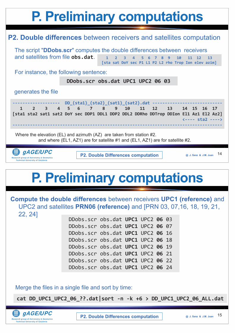
Research group of Astronomy & GeomaticsTechnical University of Catalonia
gAGE/UPC @ J. Sanz & J.M. Juan
P2. Double differences between receivers and satellites computation
14
1 2 3 4 5 6 7 8 9 10 11 12 13[sta sat DoY sec P1 L1 P2 L2 rho Trop Ion elev azim]
The script "DDobs.scr" computes the double differences between receivers and satellites from file obs.dat.
For instance, the following sentence:DDobs.scr obs.dat UPC1 UPC2 06 03
------------------- DD_{sta1}_{sta2}_{sat1}_{sat2}.dat ----------------------------1 2 3 4 5 6 7 8 9 10 11 12 13 14 15 16 17
[sta1 sta2 sat1 sat2 DoY sec DDP1 DDL1 DDP2 DDL2 DDRho DDTrop DDIon El1 Az1 El2 Az2]<---- sta2 ---->
------------------------------------------------------------------------------------
generates the file
Where the elevation (EL) and azimuth (AZ) are taken from station #2.and where (EL1, AZ1) are for satellite #1 and (EL1, AZ1) are for satellite #2.
P2. Double Differences computation
P. Preliminary computations
Research group of Astronomy & GeomaticsTechnical University of Catalonia
gAGE/UPC @ J. Sanz & J.M. Juan
Compute the double differences between receivers UPC1 (reference) and UPC2 and satellites PRN06 (reference) and [PRN 03, 07,16, 18, 19, 21, 22, 24]
15
DDobs.scr obs.dat UPC1 UPC2 06 03DDobs.scr obs.dat UPC1 UPC2 06 07DDobs.scr obs.dat UPC1 UPC2 06 16DDobs.scr obs.dat UPC1 UPC2 06 18DDobs.scr obs.dat UPC1 UPC2 06 19DDobs.scr obs.dat UPC1 UPC2 06 21DDobs.scr obs.dat UPC1 UPC2 06 22DDobs.scr obs.dat UPC1 UPC2 06 24
Merge the files in a single file and sort by time:
cat DD_UPC1_UPC2_06_??.dat|sort -n -k +6 > DD_UPC1_UPC2_06_ALL.dat
P. Preliminary computations
P2. Double Differences computation
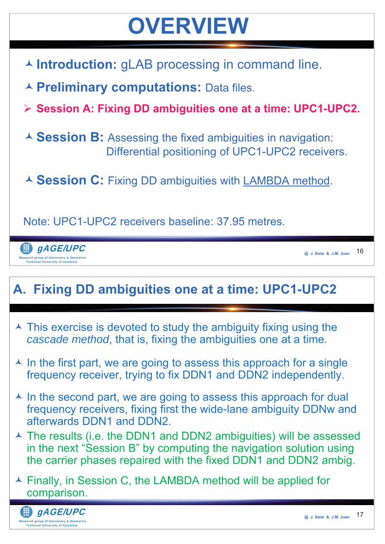
Research group of Astronomy & GeomaticsTechnical University of Catalonia
gAGE/UPC @ J. Sanz & J.M. Juan
Introduction: gLAB processing in command line.
Preliminary computations: Data files.
Session A: Fixing DD ambiguities one at a time: UPC1-UPC2.
Session B: Assessing the fixed ambiguities in navigation: Differential positioning of UPC1-UPC2 receivers.
Session C: Fixing DD ambiguities with LAMBDA method.
Note: UPC1-UPC2 receivers baseline: 37.95 metres.
OVERVIEW
16
Research group of Astronomy & GeomaticsTechnical University of Catalonia
gAGE/UPC @ J. Sanz & J.M. Juan 17
This exercise is devoted to study the ambiguity fixing using the cascade method, that is, fixing the ambiguities one at a time.
In the first part, we are going to assess this approach for a single frequency receiver, trying to fix DDN1 and DDN2 independently.
In the second part, we are going to assess this approach for dual frequency receivers, fixing first the wide-lane ambiguity DDNw and afterwards DDN1 and DDN2.The results (i.e. the DDN1 and DDN2 ambiguities) will be assessed in the next “Session B” by computing the navigation solution using the carrier phases repaired with the fixed DDN1 and DDN2 ambig.
Finally, in Session C, the LAMBDA method will be applied for comparison.
A. Fixing DD ambiguities one at a time: UPC1-UPC2
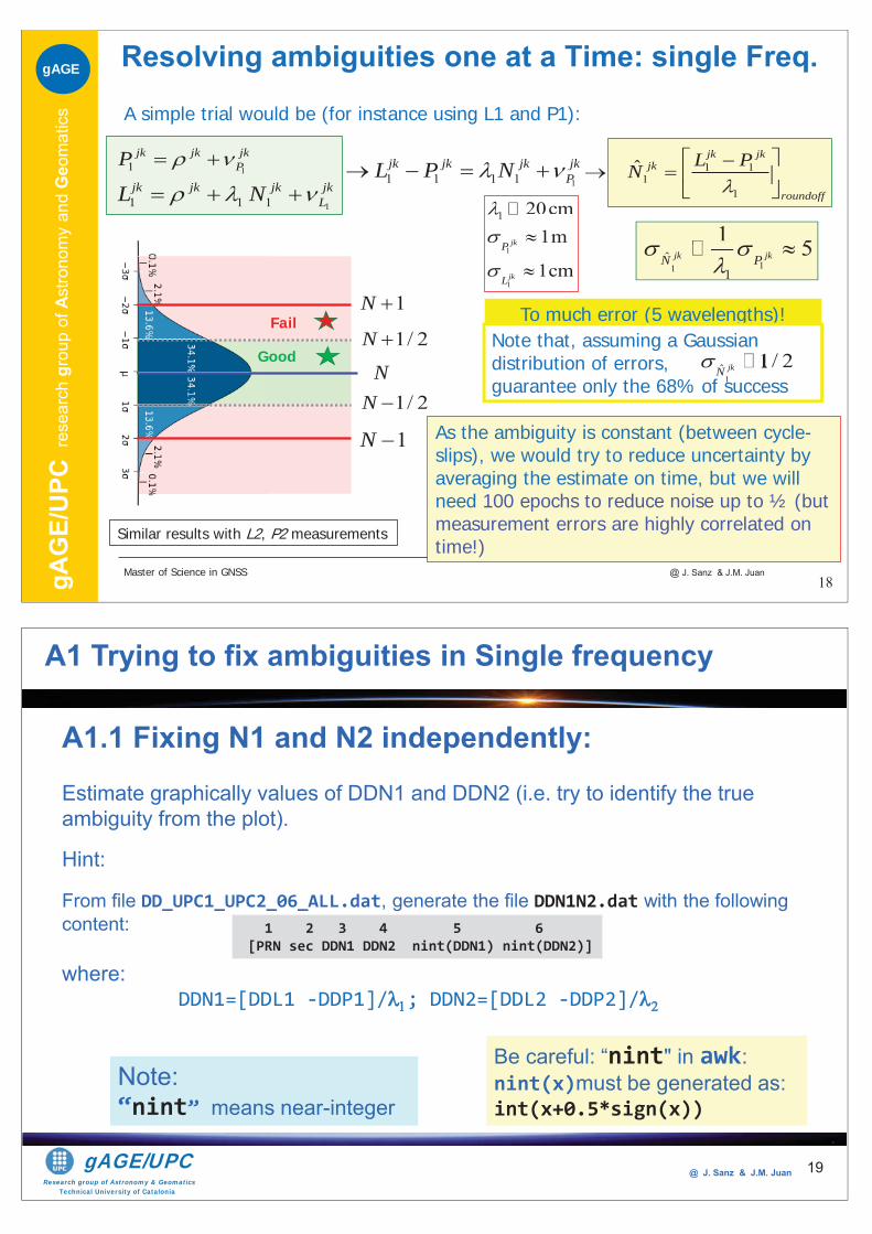
gAG
E/U
PC re
sear
ch g
roup
of A
stro
nom
y an
d G
eom
atic
sgAGE
Master of Science in GNSS @ J. Sanz & J.M. Juan
11ˆ
1
1 51jk jkN P
18
Resolving ambiguities one at a Time: single Freq.
A simple trial would be (for instance using L1 and P1):
To much error (5 wavelengths)!
11 1 1jk jk jk jk
LL N11
jk jk jkPP 1 1
11
ˆjk jk
jk
roundoff
L PN11 1 1 1
jk jk jk jkPL P N
1
1
1 20cm1m
1cm
20cmjk
jk
P
L
1N
1N
1/ 2N
1/ 2N
Note that, assuming a Gaussian distribution of errors, guarantee only the 68% of success 1
ˆ 1/ 2 1/ 2jkNN
As the ambiguity is constant (between cycle-slips), we would try to reduce uncertainty by averaging the estimate on time, but we will need 100 epochs to reduce noise up to ½ (but measurement errors are highly correlated on time!)
Good
Fail
Similar results with L2, P2 measurements
Research group of Astronomy & GeomaticsTechnical University of Catalonia
gAGE/UPC @ J. Sanz & J.M. Juan 19
A1 Trying to fix ambiguities in Single frequency
A1.1 Fixing N1 and N2 independently:Estimate graphically values of DDN1 and DDN2 (i.e. try to identify the true ambiguity from the plot).
Hint:
From file DD_UPC1_UPC2_06_ALL.dat, generate the file DDN1N2.dat with the following content:
where:DDN1=[DDL1 -DDP1]/ ; DDN2=[DDL2 -DDP2]/
1 2 3 4 5 6[PRN sec DDN1 DDN2 nint(DDN1) nint(DDN2)]
Be careful: “nint" in awk:nint(x)must be generated as: int(x+0.5*sign(x))
Note:“nint” means near-integer
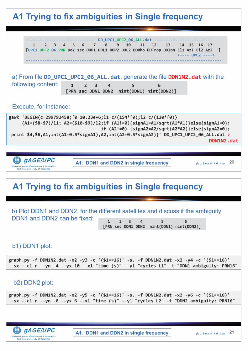
Research group of Astronomy & GeomaticsTechnical University of Catalonia
gAGE/UPC @ J. Sanz & J.M. Juan 20
a) From file DD_UPC1_UPC2_06_ALL.dat, generate the file DDN1N2.dat with the following content:
gawk 'BEGIN{c=299792458;f0=10.23e+6;l1=c/(154*f0);l2=c/(120*f0)}{A1=($8-$7)/l1; A2=($10-$9)/l2;if (A1!=0){signA1=A1/sqrt(A1*A1)}else{signA1=0};
if (A2!=0) {signA2=A2/sqrt(A2*A2)}else{signA2=0};print $4,$6,A1,int(A1+0.5*signA1),A2,int(A2+0.5*signA2)}' DD_UPC1_UPC2_06_ALL.dat >
DDN1N2.dat
A1. DDN1 and DDN2 in single frequency
1 2 3 4 5 6[PRN sec DDN1 DDN2 nint(DDN1) nint(DDN2)]
Execute, for instance:
----------------------------- DD_UPC1_UPC2_06_ALL.dat ------------------------1 2 3 4 5 6 7 8 9 10 11 12 13 14 15 16 17
[UPC1 UPC2 06 PRN DoY sec DDP1 DDL1 DDP2 DDL2 DDRho DDTrop DDIon El1 Az1 El2 Az2 ]<---- UPC2 ---->
------------------------------------------------------------------------------------
A1 Trying to fix ambiguities in Single frequency
Research group of Astronomy & GeomaticsTechnical University of Catalonia
gAGE/UPC @ J. Sanz & J.M. Juan 21
graph.py -f DDN1N2.dat -x2 -y3 -c '($1==16)' -s. -f DDN1N2.dat -x2 -y4 -c '($1==16)' -sx --cl r --yn -4 --yx 10 --xl "time (s)" --yl "cycles L1" -t "DDN1 ambiguity: PRN16"
b1) DDN1 plot:
graph.py -f DDN1N2.dat -x2 -y5 -c '($1==16)' -s. -f DDN1N2.dat -x2 -y6 -c '($1==16)' -sx --cl r --yn -8 --yx 6 --xl "time (s)" --yl "cycles L2" -t "DDN2 ambiguity: PRN16"
b2) DDN2 plot:
b) Plot DDN1 and DDN2 for the different satellites and discuss if the ambiguity DDN1 and DDN2 can be fixed: 1 2 3 4 5 6
[PRN sec DDN1 DDN2 nint(DDN1) nint(DDN2)]
A1. DDN1 and DDN2 in single frequency
A1 Trying to fix ambiguities in Single frequency
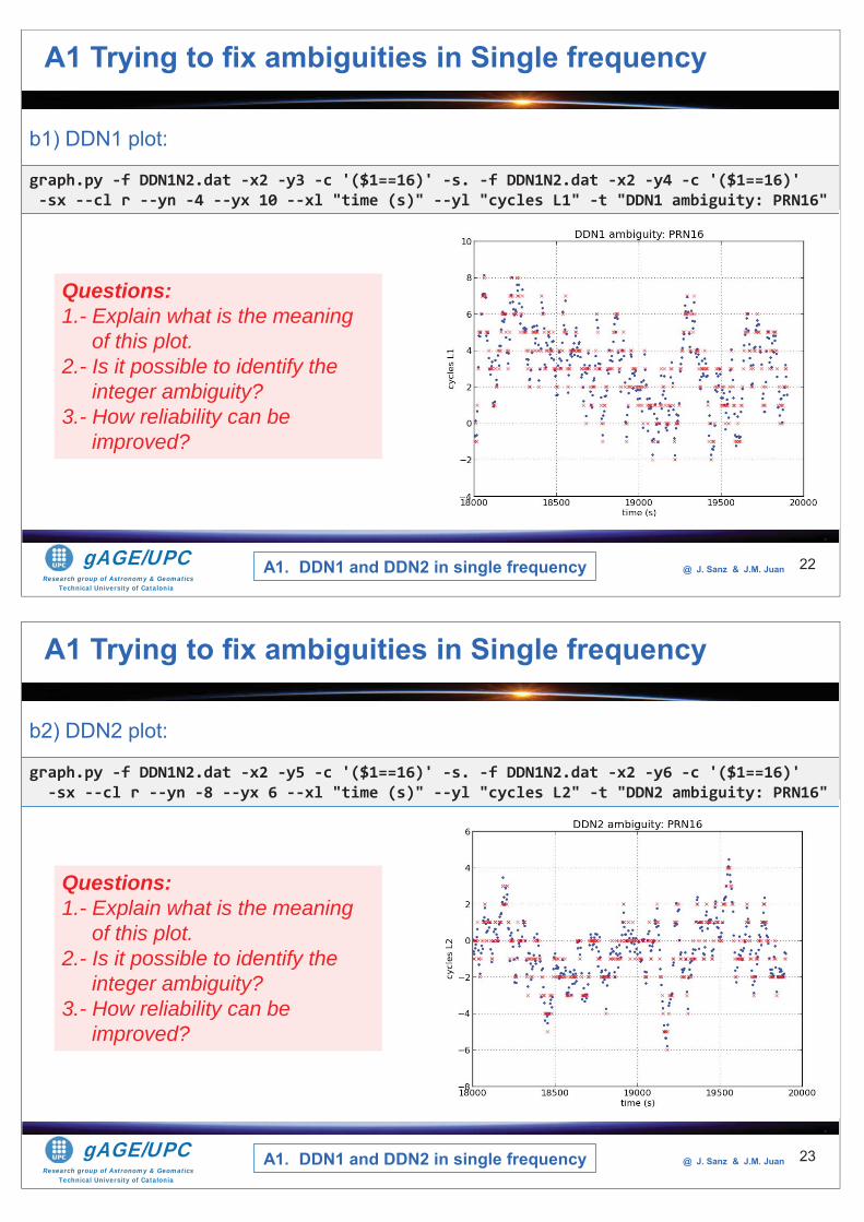
Research group of Astronomy & GeomaticsTechnical University of Catalonia
gAGE/UPC @ J. Sanz & J.M. Juan 22
b1) DDN1 plot:
graph.py -f DDN1N2.dat -x2 -y3 -c '($1==16)' -s. -f DDN1N2.dat -x2 -y4 -c '($1==16)' -sx --cl r --yn -4 --yx 10 --xl "time (s)" --yl "cycles L1" -t "DDN1 ambiguity: PRN16"
Questions:1.- Explain what is the meaning
of this plot.2.- Is it possible to identify the
integer ambiguity?3.- How reliability can be
improved?
A1. DDN1 and DDN2 in single frequency
A1 Trying to fix ambiguities in Single frequency
Research group of Astronomy & GeomaticsTechnical University of Catalonia
gAGE/UPC @ J. Sanz & J.M. Juan 23
b2) DDN2 plot:
graph.py -f DDN1N2.dat -x2 -y5 -c '($1==16)' -s. -f DDN1N2.dat -x2 -y6 -c '($1==16)' -sx --cl r --yn -8 --yx 6 --xl "time (s)" --yl "cycles L2" -t "DDN2 ambiguity: PRN16"
Questions:1.- Explain what is the meaning
of this plot.2.- Is it possible to identify the
integer ambiguity?3.- How reliability can be
improved?
A1. DDN1 and DDN2 in single frequency
A1 Trying to fix ambiguities in Single frequency
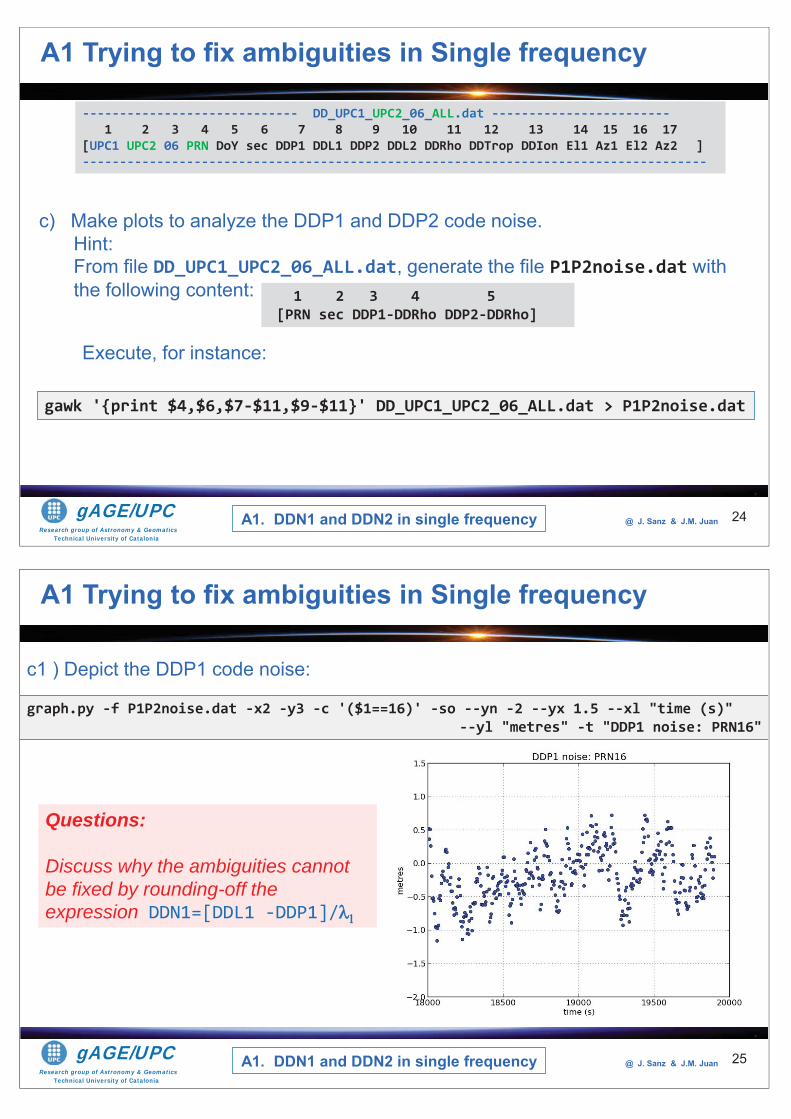
Research group of Astronomy & GeomaticsTechnical University of Catalonia
gAGE/UPC @ J. Sanz & J.M. Juan 24
c) Make plots to analyze the DDP1 and DDP2 code noise.Hint:From file DD_UPC1_UPC2_06_ALL.dat, generate the file P1P2noise.dat with the following content:
gawk '{print $4,$6,$7-$11,$9-$11}' DD_UPC1_UPC2_06_ALL.dat > P1P2noise.dat
----------------------------- DD_UPC1_UPC2_06_ALL.dat ------------------------1 2 3 4 5 6 7 8 9 10 11 12 13 14 15 16 17
[UPC1 UPC2 06 PRN DoY sec DDP1 DDL1 DDP2 DDL2 DDRho DDTrop DDIon El1 Az1 El2 Az2 ]------------------------------------------------------------------------------------
Execute, for instance:
1 2 3 4 5[PRN sec DDP1-DDRho DDP2-DDRho]
A1. DDN1 and DDN2 in single frequency
A1 Trying to fix ambiguities in Single frequency
Research group of Astronomy & GeomaticsTechnical University of Catalonia
gAGE/UPC @ J. Sanz & J.M. Juan 25
c1 ) Depict the DDP1 code noise:
graph.py -f P1P2noise.dat -x2 -y3 -c '($1==16)' -so --yn -2 --yx 1.5 --xl "time (s)" --yl "metres" -t "DDP1 noise: PRN16"
Questions:
Discuss why the ambiguities cannot be fixed by rounding-off the expression DDN1=[DDL1 -DDP1]/
A1. DDN1 and DDN2 in single frequency
A1 Trying to fix ambiguities in Single frequency
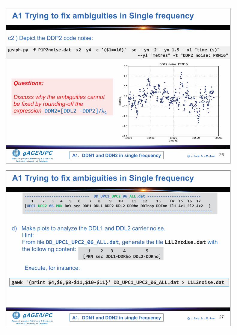
Research group of Astronomy & GeomaticsTechnical University of Catalonia
gAGE/UPC @ J. Sanz & J.M. Juan 26
c2 ) Depict the DDP2 code noise:
graph.py -f P1P2noise.dat -x2 -y4 -c '($1==16)' -so --yn -2 --yx 1.5 --xl "time (s)" --yl "metres" -t "DDP2 noise: PRN16"
A1. DDN1 and DDN2 in single frequency
A1 Trying to fix ambiguities in Single frequency
Questions:
Discuss why the ambiguities cannot be fixed by rounding-off the expression DDN2=[DDL2 –DDP2]/
Research group of Astronomy & GeomaticsTechnical University of Catalonia
gAGE/UPC @ J. Sanz & J.M. Juan 27
d) Make plots to analyze the DDL1 and DDL2 carrier noise.Hint:From file DD_UPC1_UPC2_06_ALL.dat, generate the file L1L2noise.dat with the following content:
gawk '{print $4,$6,$8-$11,$10-$11}' DD_UPC1_UPC2_06_ALL.dat > L1L2noise.dat
----------------------------- DD_UPC1_UPC2_06_ALL.dat ------------------------1 2 3 4 5 6 7 8 9 10 11 12 13 14 15 16 17
[UPC1 UPC2 06 PRN DoY sec DDP1 DDL1 DDP2 DDL2 DDRho DDTrop DDIon El1 Az1 El2 Az2 ]------------------------------------------------------------------------------------
Execute, for instance:
1 2 3 4 5[PRN sec DDL1-DDRho DDL2-DDRho]
A1. DDN1 and DDN2 in single frequency
A1 Trying to fix ambiguities in Single frequency
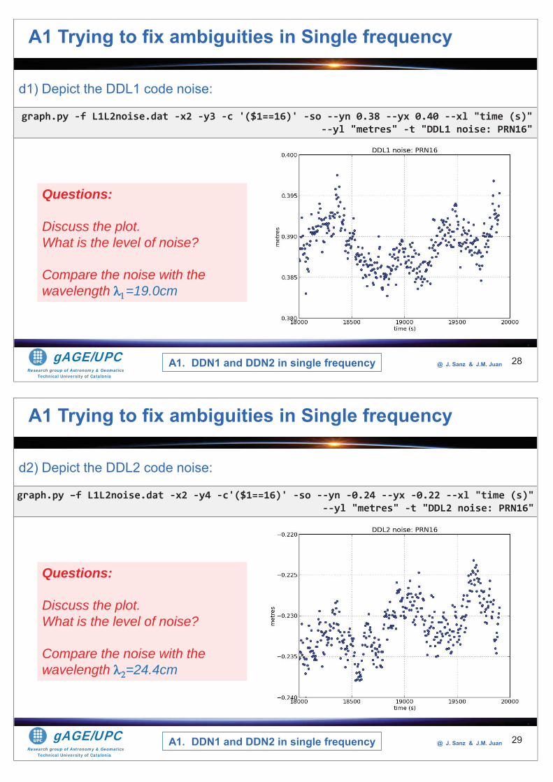
Research group of Astronomy & GeomaticsTechnical University of Catalonia
gAGE/UPC @ J. Sanz & J.M. Juan 28
d1) Depict the DDL1 code noise:
graph.py -f L1L2noise.dat -x2 -y3 -c '($1==16)' -so --yn 0.38 --yx 0.40 --xl "time (s)" --yl "metres" -t "DDL1 noise: PRN16"
Questions:
Discuss the plot.What is the level of noise?
Compare the noise with the wavelength =19.0cm
A1. DDN1 and DDN2 in single frequency
A1 Trying to fix ambiguities in Single frequency
Research group of Astronomy & GeomaticsTechnical University of Catalonia
gAGE/UPC @ J. Sanz & J.M. Juan 29
d2) Depict the DDL2 code noise:
graph.py –f L1L2noise.dat -x2 -y4 -c'($1==16)' -so --yn -0.24 --yx -0.22 --xl "time (s)" --yl "metres" -t "DDL2 noise: PRN16"
Questions:
Discuss the plot.What is the level of noise?
Compare the noise with the wavelength =24.4cm
A1. DDN1 and DDN2 in single frequency
A1 Trying to fix ambiguities in Single frequency
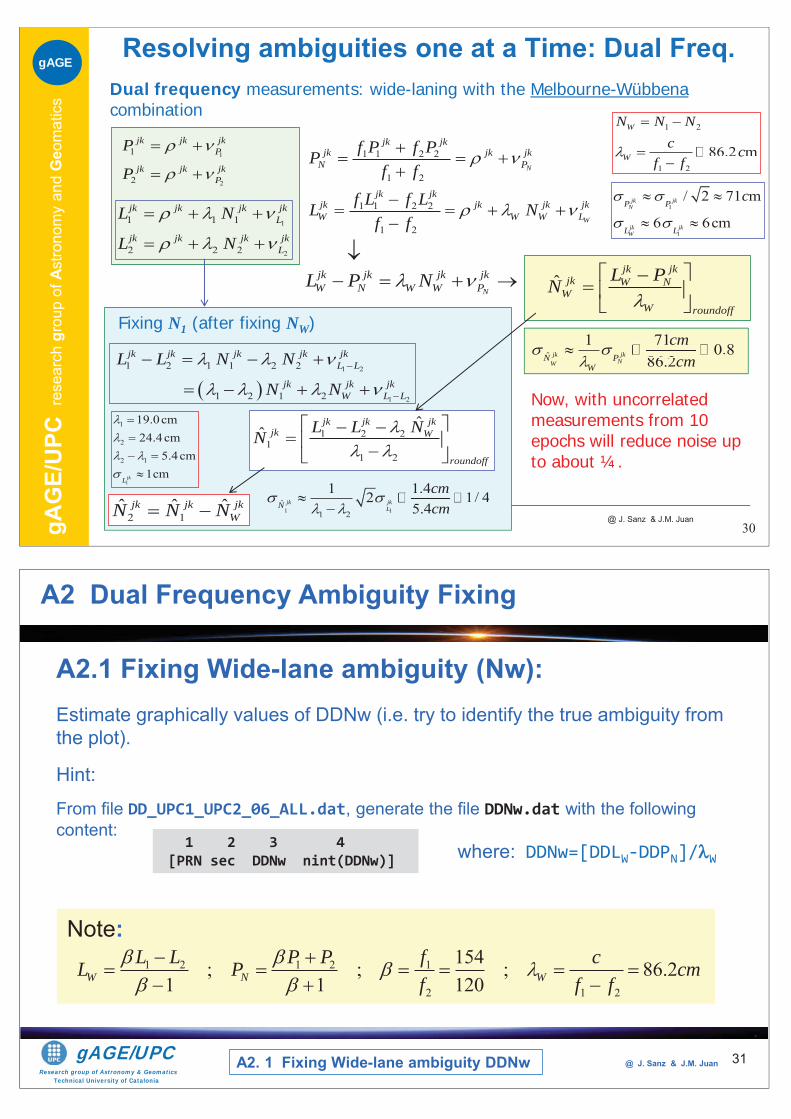
gAG
E/U
PC re
sear
ch g
roup
of A
stro
nom
y an
d G
eom
atic
sgAGE
Master of Science in GNSS @ J. Sanz & J.M. Juan30
Resolving ambiguities one at a Time: Dual Freq. Dual frequency measurements: wide-laning with the Melbourne-Wübbenacombination
1
2
1 1 1
2 2 2
jk jk jk jkL
jk jk jk jkL
L N
L N
1
2
1
2
jk jk jkP
jk jk jkP
P
P
ˆjk jk
jk W NW
W roundoff
L PN
1 1 2 2
1 2
1 1 2 2
1 2
N
W
jk jkjk jk jk
N P
jk jkjk jk jk jkW W W L
f P f PPf f
f L f LL Nf f
1 2
1 2
86.2 m86.2 m
W
W
N N Nc c
f f
Now, with uncorrelated measurements from 10 epochs will reduce noise up to about ¼.
ˆ1 71 0.8
86.271 0.8
86 2jk jkNW
N PW
cmcm
N
jk jk jk jkW N W W PL P N
1 2
1 2
1 2 1 1 2 2
1 2 1 2
jk jk jk jk jkL L
jk jk jkW L L
L L N N
N N
1
1
/ 2 71 m
6 6cm
jk jkN
jk jkW
P P
L L
c
1 2 21
1 2
ˆˆjk jk jk
jk W
roundoff
L L NN
Fixing N1 (after fixing NW)
1 1ˆ
1 2
1 1.42 1/ 45.41.4 1/ 41.45 4jk jk
LN
cmcm
2 1ˆ ˆ ˆjk jk jk
WN N N
1
1
2
2 1
19.0cm24.4cm
5.4cm1cmjkL
Research group of Astronomy & GeomaticsTechnical University of Catalonia
gAGE/UPC @ J. Sanz & J.M. Juan 31
A2 Dual Frequency Ambiguity Fixing
A2.1 Fixing Wide-lane ambiguity (Nw):Estimate graphically values of DDNw (i.e. try to identify the true ambiguity from the plot).
Hint:
From file DD_UPC1_UPC2_06_ALL.dat, generate the file DDNw.dat with the following content:
where: DDNw=[DDLW-DDPN]/ W1 2 3 4
[PRN sec DDNw nint(DDNw)]
1 2 1 2 1
2 1 2
154; ; ; 86.21 1 120W N W
L L P P f cL P cmf f f
Note:
A2. 1 Fixing Wide-lane ambiguity DDNw

Research group of Astronomy & GeomaticsTechnical University of Catalonia
gAGE/UPC @ J. Sanz & J.M. Juan 32
a) From file DD_UPC1_UPC2_06_ALL.dat, generate the file DDNw.dat with the following content: where: DDNw=[DDLW-DDPN]/ W
cat DD_UPC1_UPC2_06_ALL.dat| gawk 'BEGIN{s12=154/120} {mw=(s12*$8-$10)/(s12-1)-(s12*$7+$9)/(s12+1);if(mw!=0){sign=mw/sqrt(mw*mw)} else{sign=0};printf "%02i %i %14.4f %i \n", $4,$6, mw/0.862,int(mw/0.862+0.5*sign)}'>
DDNw.dat
Execute, for instance:
----------------------------- DD_UPC1_UPC2_06_ALL.dat ------------------------1 2 3 4 5 6 7 8 9 10 11 12 13 14 15 16 17
[UPC1 UPC2 06 PRN DoY sec DDP1 DDL1 DDP2 DDL2 DDRho DDTrop DDIon El1 Az1 El2 Az2 ]------------------------------------------------------------------------------------
1 2 3 4[PRN sec DDNw nint(DDNw)]
A2 Dual Frequency Ambiguity Fixing
A2. 1 Fixing Wide-lane ambiguity DDNw
Research group of Astronomy & GeomaticsTechnical University of Catalonia
gAGE/UPC @ J. Sanz & J.M. Juan 33
graph.py -f DDNw.dat -x2 -y3 -c '($1==03)' -s. -f DDNw.dat -x2 -y4 -c '($1==03)' -sx --cl r --yn -1 --yx 7 --xl "time (s)" --yl "cycles Lw" -t "DDNw ambiguity: PRN03"
b) Plot DDNw for the different satellites and discuss if the ambiguity DDNw can be fixed: 1 2 3 4
[PRN sec DDNw nint(DDNw)]
graph.py -f DDNw.dat -x2 -y3 -c '($1==07)' -s. -f DDNw.dat -x2 -y4 -c '($1==07)' -sx --cl r --yn -4 --yx 4 --xl "time (s)" --yl "cycles Lw" -t "DDNw ambiguity: PRN07"
- Example PRN03 plot:
- Example PRN07 plot:
A2 Dual Frequency Ambiguity Fixing
A2. 1 Fixing Wide-lane ambiguity DDNw
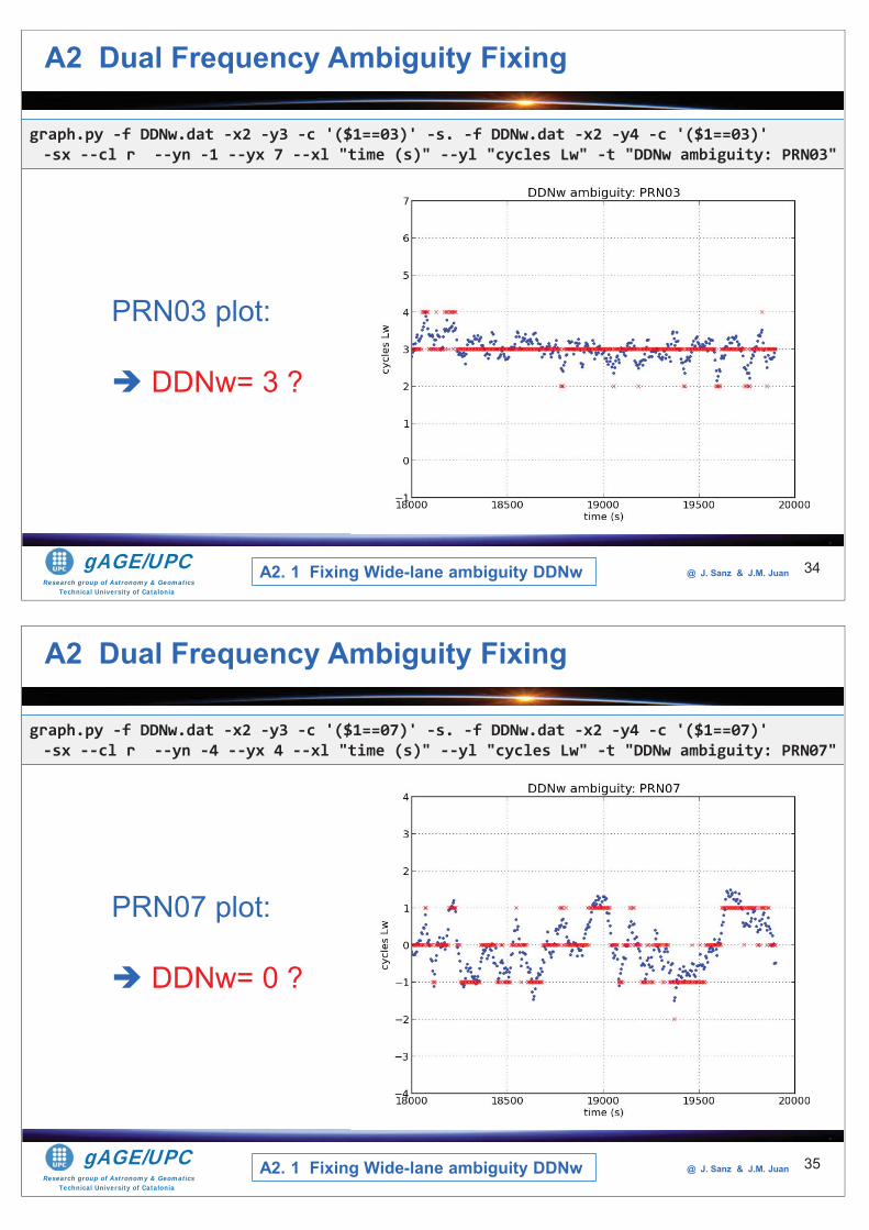
Research group of Astronomy & GeomaticsTechnical University of Catalonia
gAGE/UPC @ J. Sanz & J.M. Juan 34
graph.py -f DDNw.dat -x2 -y3 -c '($1==03)' -s. -f DDNw.dat -x2 -y4 -c '($1==03)' -sx --cl r --yn -1 --yx 7 --xl "time (s)" --yl "cycles Lw" -t "DDNw ambiguity: PRN03"
PRN03 plot:
DDNw= 3 ?
A2 Dual Frequency Ambiguity Fixing
A2. 1 Fixing Wide-lane ambiguity DDNw
Research group of Astronomy & GeomaticsTechnical University of Catalonia
gAGE/UPC @ J. Sanz & J.M. Juan 35
PRN07 plot:
DDNw= 0 ?
A2 Dual Frequency Ambiguity Fixing
A2. 1 Fixing Wide-lane ambiguity DDNw
graph.py -f DDNw.dat -x2 -y3 -c '($1==07)' -s. -f DDNw.dat -x2 -y4 -c '($1==07)' -sx --cl r --yn -4 --yx 4 --xl "time (s)" --yl "cycles Lw" -t "DDNw ambiguity: PRN07"
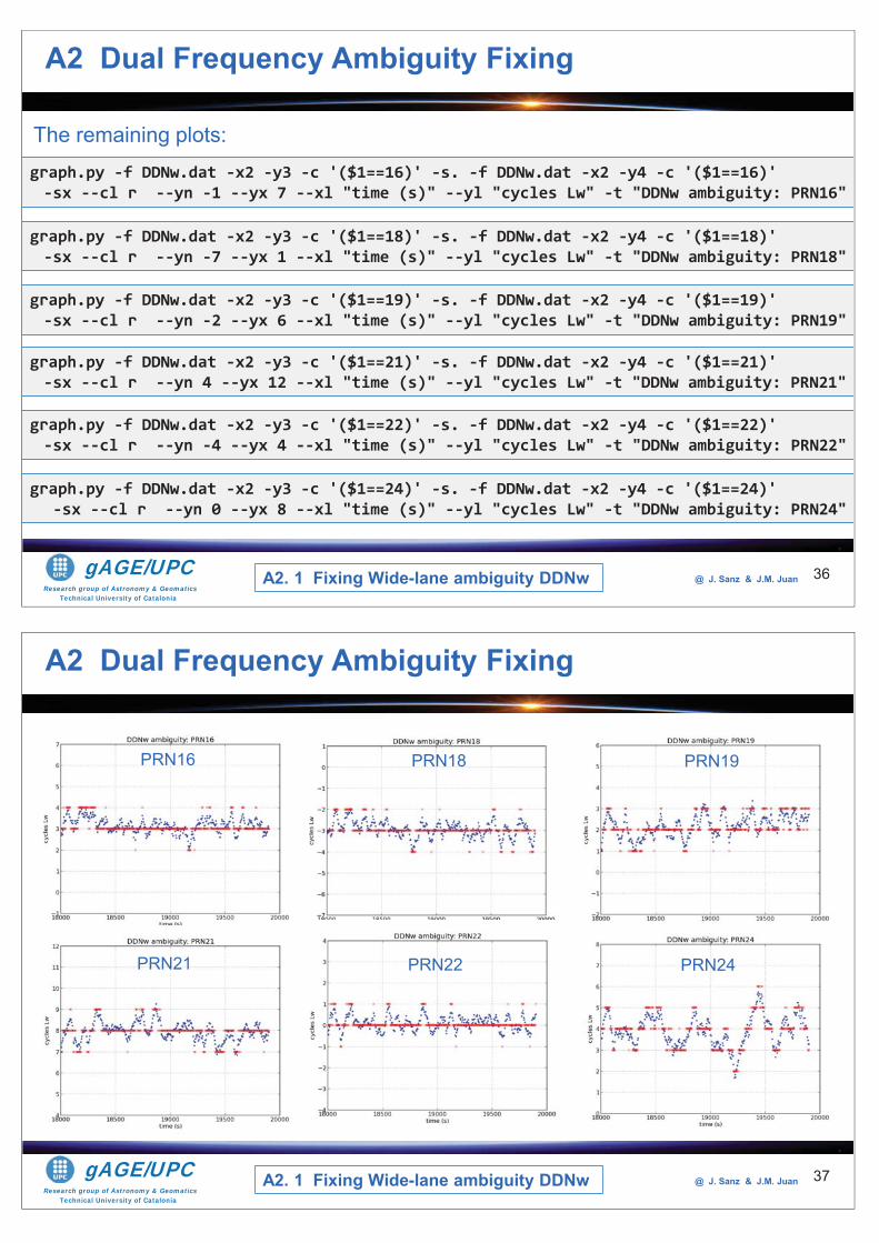
Research group of Astronomy & GeomaticsTechnical University of Catalonia
gAGE/UPC @ J. Sanz & J.M. Juan 36
graph.py -f DDNw.dat -x2 -y3 -c '($1==19)' -s. -f DDNw.dat -x2 -y4 -c '($1==19)' -sx --cl r --yn -2 --yx 6 --xl "time (s)" --yl "cycles Lw" -t "DDNw ambiguity: PRN19"
graph.py -f DDNw.dat -x2 -y3 -c '($1==21)' -s. -f DDNw.dat -x2 -y4 -c '($1==21)' -sx --cl r --yn 4 --yx 12 --xl "time (s)" --yl "cycles Lw" -t "DDNw ambiguity: PRN21"
graph.py -f DDNw.dat -x2 -y3 -c '($1==22)' -s. -f DDNw.dat -x2 -y4 -c '($1==22)' -sx --cl r --yn -4 --yx 4 --xl "time (s)" --yl "cycles Lw" -t "DDNw ambiguity: PRN22"
graph.py -f DDNw.dat -x2 -y3 -c '($1==24)' -s. -f DDNw.dat -x2 -y4 -c '($1==24)' -sx --cl r --yn 0 --yx 8 --xl "time (s)" --yl "cycles Lw" -t "DDNw ambiguity: PRN24"
graph.py -f DDNw.dat -x2 -y3 -c '($1==16)' -s. -f DDNw.dat -x2 -y4 -c '($1==16)' -sx --cl r --yn -1 --yx 7 --xl "time (s)" --yl "cycles Lw" -t "DDNw ambiguity: PRN16"
graph.py -f DDNw.dat -x2 -y3 -c '($1==18)' -s. -f DDNw.dat -x2 -y4 -c '($1==18)' -sx --cl r --yn -7 --yx 1 --xl "time (s)" --yl "cycles Lw" -t "DDNw ambiguity: PRN18"
The remaining plots:
A2 Dual Frequency Ambiguity Fixing
A2. 1 Fixing Wide-lane ambiguity DDNw
Research group of Astronomy & GeomaticsTechnical University of Catalonia
gAGE/UPC @ J. Sanz & J.M. Juan 37
A2 Dual Frequency Ambiguity Fixing
A2. 1 Fixing Wide-lane ambiguity DDNw
PRN16 PRN18 PRN19
PRN21 PRN22 PRN24
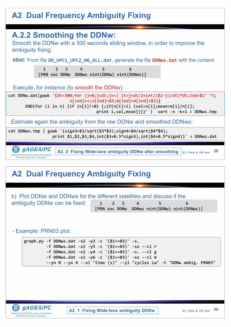
Research group of Astronomy & GeomaticsTechnical University of Catalonia
gAGE/UPC @ J. Sanz & J.M. Juan 38
Hint: From file DD_UPC1_UPC2_06_ALL.dat, generate the file DDNws.dat with the content:
cat DDNw.dat|gawk '{dt=300;for (j=0;j<dt;j++) {t=j+dt/2+int(($2-j)/dt)*dt;ind=$1" "t; n[ind]++;v[ind]=$3;m[ind]=m[ind]+$3}}
END{for (i in n) {if (n[i]!=0) {;if(n[i]>1) {val=v[i];mean=m[i]/n[i]; print i,val,mean}}}}' | sort -n -k+1 > DDNws.tmp
Execute, for instance (to smooth the DDNw):
1 2 3 4 5 6 [PRN sec DDNw DDNws nint(DDNw) nint(DDNws)]
A.2.2 Smoothing the DDNw:Smooth the DDNw with a 300 seconds sliding window, in order to improve the ambiguity fixing.
cat DDNws.tmp | gawk '{sign3=$3/sqrt($3*$3);sign4=$4/sqrt($4*$4);print $1,$2,$3,$4,int($3+0.5*sign3),int($4+0.5*sign4)}' > DDNws.dat
Estimate again the ambiguity from the raw DDNw and smoothed DDNws:
A2 Dual Frequency Ambiguity Fixing
A2. 2 Fixing Wide-lane ambiguity DDNw after smoothing
Research group of Astronomy & GeomaticsTechnical University of Catalonia
gAGE/UPC @ J. Sanz & J.M. Juan 39
graph.py -f DDNws.dat -x2 -y3 -c '($1==03)' -s. -f DDNws.dat -x2 -y5 -c '($1==03)' -sx --cl r -f DDNws.dat -x2 -y4 -c '($1==03)' -s. --cl g -f DDNws.dat -x2 -y6 -c '($1==03)' -sx --cl m --yn 0 --yx 6 --xl "time (s)" --yl "cycles Lw" -t "DDNw ambig. PRN03"
b) Plot DDNw and DDNws for the different satellites and discuss if the ambiguity DDNw can be fixed:
- Example: PRN03 plot:
1 2 3 4 5 6 [PRN sec DDNw DDNws nint(DDNw) nint(DDNws)]
A2 Dual Frequency Ambiguity Fixing
A2. 1 Fixing Wide-lane ambiguity DDNw
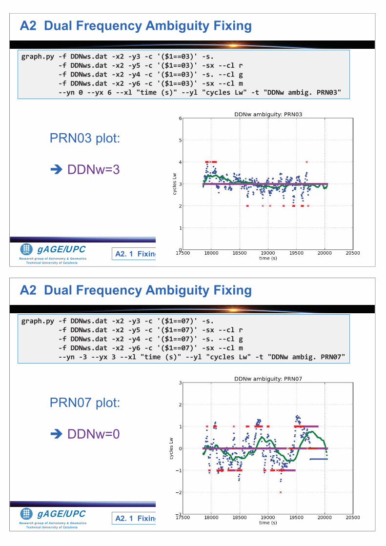
Research group of Astronomy & GeomaticsTechnical University of Catalonia
gAGE/UPC @ J. Sanz & J.M. Juan 40
graph.py -f DDNws.dat -x2 -y3 -c '($1==03)' -s. -f DDNws.dat -x2 -y5 -c '($1==03)' -sx --cl r -f DDNws.dat -x2 -y4 -c '($1==03)' -s. --cl g -f DDNws.dat -x2 -y6 -c '($1==03)' -sx --cl m --yn 0 --yx 6 --xl "time (s)" --yl "cycles Lw" -t "DDNw ambig. PRN03"
PRN03 plot:
DDNw=3
A2 Dual Frequency Ambiguity Fixing
A2. 1 Fixing Wide-lane ambiguity DDNw
Research group of Astronomy & GeomaticsTechnical University of Catalonia
gAGE/UPC @ J. Sanz & J.M. Juan 41
graph.py -f DDNws.dat -x2 -y3 -c '($1==07)' -s. -f DDNws.dat -x2 -y5 -c '($1==07)' -sx --cl r -f DDNws.dat -x2 -y4 -c '($1==07)' -s. --cl g -f DDNws.dat -x2 -y6 -c '($1==07)' -sx --cl m --yn -3 --yx 3 --xl "time (s)" --yl "cycles Lw" -t "DDNw ambig. PRN07"
PRN07 plot:
DDNw=0
A2 Dual Frequency Ambiguity Fixing
A2. 1 Fixing Wide-lane ambiguity DDNw
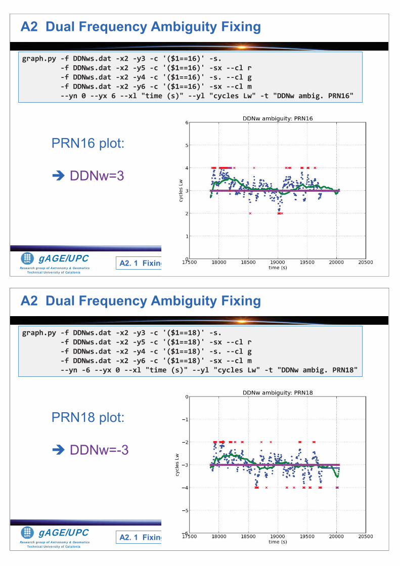
Research group of Astronomy & GeomaticsTechnical University of Catalonia
gAGE/UPC @ J. Sanz & J.M. Juan 42
graph.py -f DDNws.dat -x2 -y3 -c '($1==16)' -s. -f DDNws.dat -x2 -y5 -c '($1==16)' -sx --cl r -f DDNws.dat -x2 -y4 -c '($1==16)' -s. --cl g -f DDNws.dat -x2 -y6 -c '($1==16)' -sx --cl m --yn 0 --yx 6 --xl "time (s)" --yl "cycles Lw" -t "DDNw ambig. PRN16"
PRN16 plot:
DDNw=3
A2 Dual Frequency Ambiguity Fixing
A2. 1 Fixing Wide-lane ambiguity DDNw
Research group of Astronomy & GeomaticsTechnical University of Catalonia
gAGE/UPC @ J. Sanz & J.M. Juan 43
graph.py -f DDNws.dat -x2 -y3 -c '($1==18)' -s. -f DDNws.dat -x2 -y5 -c '($1==18)' -sx --cl r -f DDNws.dat -x2 -y4 -c '($1==18)' -s. --cl g -f DDNws.dat -x2 -y6 -c '($1==18)' -sx --cl m --yn -6 --yx 0 --xl "time (s)" --yl "cycles Lw" -t "DDNw ambig. PRN18"
PRN18 plot:
DDNw=-3
A2 Dual Frequency Ambiguity Fixing
A2. 1 Fixing Wide-lane ambiguity DDNw
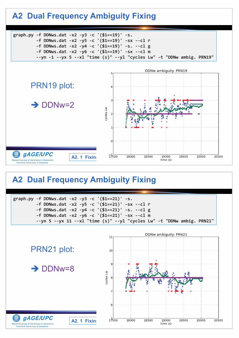
Research group of Astronomy & GeomaticsTechnical University of Catalonia
gAGE/UPC @ J. Sanz & J.M. Juan 44
graph.py -f DDNws.dat -x2 -y3 -c '($1==19)' -s. -f DDNws.dat -x2 -y5 -c '($1==19)' -sx --cl r -f DDNws.dat -x2 -y4 -c '($1==19)' -s. --cl g -f DDNws.dat -x2 -y6 -c '($1==19)' -sx --cl m --yn -1 --yx 5 --xl "time (s)" --yl "cycles Lw" -t "DDNw ambig. PRN19"
PRN19 plot:
DDNw=2
A2 Dual Frequency Ambiguity Fixing
A2. 1 Fixing Wide-lane ambiguity DDNw
Research group of Astronomy & GeomaticsTechnical University of Catalonia
gAGE/UPC @ J. Sanz & J.M. Juan 45
graph.py -f DDNws.dat -x2 -y3 -c '($1==21)' -s. -f DDNws.dat -x2 -y5 -c '($1==21)' -sx --cl r -f DDNws.dat -x2 -y4 -c '($1==21)' -s. --cl g -f DDNws.dat -x2 -y6 -c '($1==21)' -sx --cl m --yn 5 --yx 11 --xl "time (s)" --yl "cycles Lw" -t "DDNw ambig. PRN21"
PRN21 plot:
DDNw=8
A2 Dual Frequency Ambiguity Fixing
A2. 1 Fixing Wide-lane ambiguity DDNw
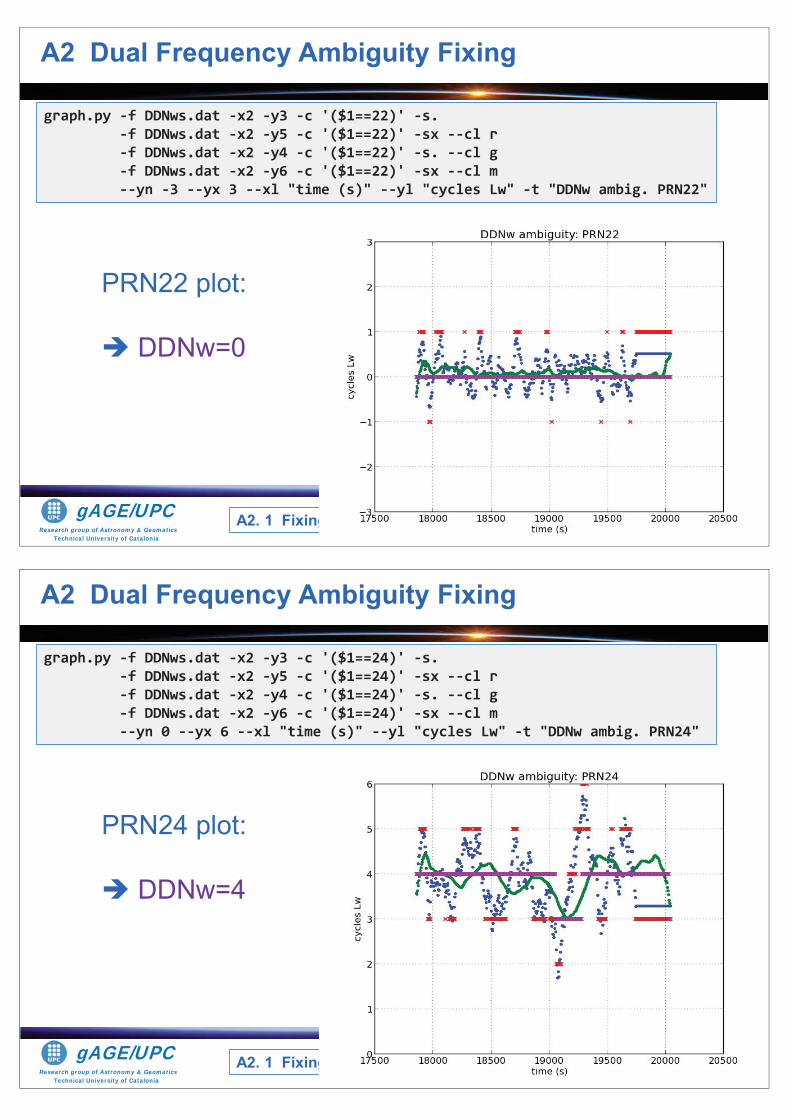
Research group of Astronomy & GeomaticsTechnical University of Catalonia
gAGE/UPC @ J. Sanz & J.M. Juan 46
graph.py -f DDNws.dat -x2 -y3 -c '($1==22)' -s. -f DDNws.dat -x2 -y5 -c '($1==22)' -sx --cl r -f DDNws.dat -x2 -y4 -c '($1==22)' -s. --cl g -f DDNws.dat -x2 -y6 -c '($1==22)' -sx --cl m --yn -3 --yx 3 --xl "time (s)" --yl "cycles Lw" -t "DDNw ambig. PRN22"
PRN22 plot:
DDNw=0
A2 Dual Frequency Ambiguity Fixing
A2. 1 Fixing Wide-lane ambiguity DDNw
Research group of Astronomy & GeomaticsTechnical University of Catalonia
gAGE/UPC @ J. Sanz & J.M. Juan 47
PRN24 plot:
DDNw=4
graph.py -f DDNws.dat -x2 -y3 -c '($1==24)' -s. -f DDNws.dat -x2 -y5 -c '($1==24)' -sx --cl r -f DDNws.dat -x2 -y4 -c '($1==24)' -s. --cl g -f DDNws.dat -x2 -y6 -c '($1==24)' -sx --cl m --yn 0 --yx 6 --xl "time (s)" --yl "cycles Lw" -t "DDNw ambig. PRN24"
A2 Dual Frequency Ambiguity Fixing
A2. 1 Fixing Wide-lane ambiguity DDNw
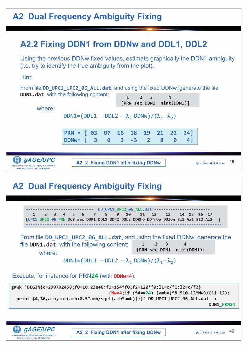
Research group of Astronomy & GeomaticsTechnical University of Catalonia
gAGE/UPC @ J. Sanz & J.M. Juan 48
A2 Dual Frequency Ambiguity Fixing
A2.2 Fixing DDN1 from DDNw and DDL1, DDL2Using the previous DDNw fixed values, estimate graphically the DDN1 ambiguity (i.e. try to identify the true ambiguity from the plot).
Hint:
From file DD_UPC1_UPC2_06_ALL.dat, and using the fixed DDNw, generate the file DDN1.dat with the following content:
where:DDN1=(DDL1 DDL2 2 DDNw)/( 1 2)
1 2 3 4[PRN sec DDN1 nint(DDN1)]
PRN = [ 03 07 16 18 19 21 22 24]DDNw= [ 3 0 3 -3 2 8 0 4]
A2. 2 Fixing DDN1 after fixing DDNw
Research group of Astronomy & GeomaticsTechnical University of Catalonia
gAGE/UPC @ J. Sanz & J.M. Juan 49
gawk 'BEGIN{c=299792458;f0=10.23e+6;f1=154*f0;f2=120*f0;l1=c/f1;l2=c/f2}{Nw=4;if ($4==24) {amb=($8-$10-l2*Nw)/(l1-l2);
print $4,$6,amb,int(amb+0.5*amb/sqrt(amb*amb))}}' DD_UPC1_UPC2_06_ALL.dat > DDN1_PRN24
Execute, for instance for PRN24 (with DDNw=4):
----------------------------- DD_UPC1_UPC2_06_ALL.dat ------------------------1 2 3 4 5 6 7 8 9 10 11 12 13 14 15 16 17
[UPC1 UPC2 06 PRN DoY sec DDP1 DDL1 DDP2 DDL2 DDRho DDTrop DDIon El1 Az1 El2 Az2 ]------------------------------------------------------------------------------------
From file DD_UPC1_UPC2_06_ALL.dat, and using the fixed DDNw, generate the file DDN1.dat with the following content:
where:DDN1=(DDL1 DDL2 2 DDNw)/( 1 2)
1 2 3 4[PRN sec DDN1 nint(DDN1)]
A2 Dual Frequency Ambiguity Fixing
A2. 2 Fixing DDN1 after fixing DDNw
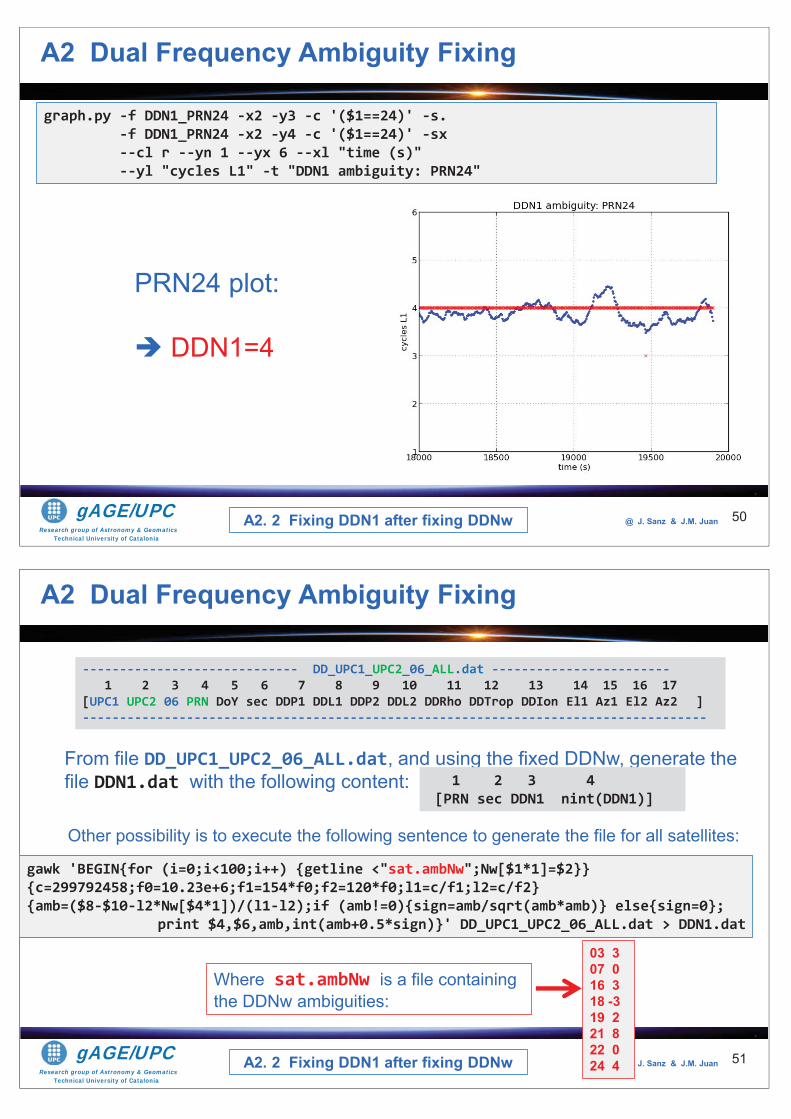
Research group of Astronomy & GeomaticsTechnical University of Catalonia
gAGE/UPC @ J. Sanz & J.M. Juan 50
graph.py -f DDN1_PRN24 -x2 -y3 -c '($1==24)' -s. -f DDN1_PRN24 -x2 -y4 -c '($1==24)' -sx --cl r --yn 1 --yx 6 --xl "time (s)" --yl "cycles L1" -t "DDN1 ambiguity: PRN24"
A2 Dual Frequency Ambiguity Fixing
A2. 2 Fixing DDN1 after fixing DDNw
PRN24 plot:
DDN1=4
Research group of Astronomy & GeomaticsTechnical University of Catalonia
gAGE/UPC @ J. Sanz & J.M. Juan 51
gawk 'BEGIN{for (i=0;i<100;i++) {getline <"sat.ambNw";Nw[$1*1]=$2}} {c=299792458;f0=10.23e+6;f1=154*f0;f2=120*f0;l1=c/f1;l2=c/f2}{amb=($8-$10-l2*Nw[$4*1])/(l1-l2);if (amb!=0){sign=amb/sqrt(amb*amb)} else{sign=0};
print $4,$6,amb,int(amb+0.5*sign)}' DD_UPC1_UPC2_06_ALL.dat > DDN1.dat
Other possibility is to execute the following sentence to generate the file for all satellites:
----------------------------- DD_UPC1_UPC2_06_ALL.dat ------------------------1 2 3 4 5 6 7 8 9 10 11 12 13 14 15 16 17
[UPC1 UPC2 06 PRN DoY sec DDP1 DDL1 DDP2 DDL2 DDRho DDTrop DDIon El1 Az1 El2 Az2 ]------------------------------------------------------------------------------------
From file DD_UPC1_UPC2_06_ALL.dat, and using the fixed DDNw, generate the file DDN1.dat with the following content: 1 2 3 4
[PRN sec DDN1 nint(DDN1)]
Where sat.ambNw is a file containing the DDNw ambiguities:
03 307 016 318 -319 2 21 822 024 4
A2 Dual Frequency Ambiguity Fixing
A2. 2 Fixing DDN1 after fixing DDNw
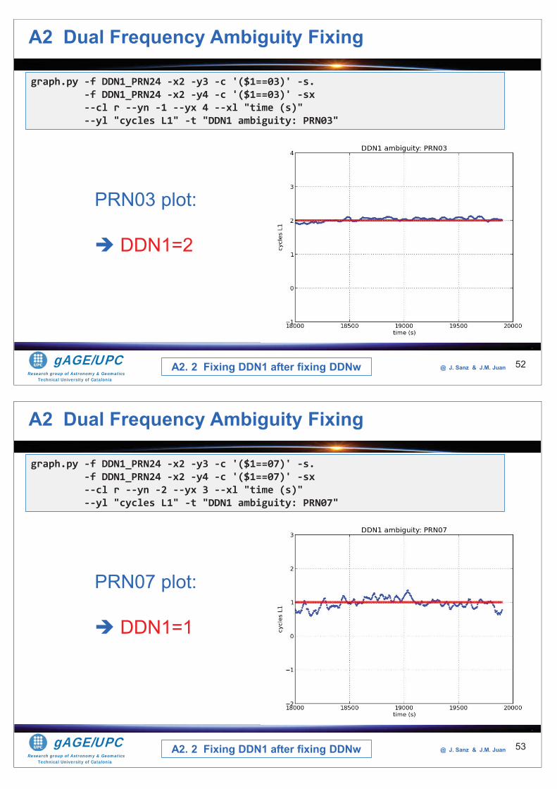
Research group of Astronomy & GeomaticsTechnical University of Catalonia
gAGE/UPC @ J. Sanz & J.M. Juan 52
graph.py -f DDN1_PRN24 -x2 -y3 -c '($1==03)' -s. -f DDN1_PRN24 -x2 -y4 -c '($1==03)' -sx --cl r --yn -1 --yx 4 --xl "time (s)" --yl "cycles L1" -t "DDN1 ambiguity: PRN03"
A2 Dual Frequency Ambiguity Fixing
A2. 2 Fixing DDN1 after fixing DDNw
PRN03 plot:
DDN1=2
Research group of Astronomy & GeomaticsTechnical University of Catalonia
gAGE/UPC @ J. Sanz & J.M. Juan 53
PRN07 plot:
DDN1=1
graph.py -f DDN1_PRN24 -x2 -y3 -c '($1==07)' -s. -f DDN1_PRN24 -x2 -y4 -c '($1==07)' -sx --cl r --yn -2 --yx 3 --xl "time (s)" --yl "cycles L1" -t "DDN1 ambiguity: PRN07"
A2 Dual Frequency Ambiguity Fixing
A2. 2 Fixing DDN1 after fixing DDNw
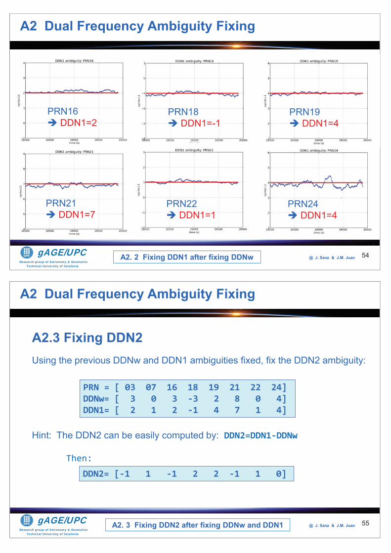
Research group of Astronomy & GeomaticsTechnical University of Catalonia
gAGE/UPC @ J. Sanz & J.M. Juan 54
A2 Dual Frequency Ambiguity Fixing
A2. 2 Fixing DDN1 after fixing DDNw
PRN16DDN1=2
PRN18DDN1=-1
PRN19DDN1=4
PRN21DDN1=7
PRN22DDN1=1
PRN24DDN1=4
Research group of Astronomy & GeomaticsTechnical University of Catalonia
gAGE/UPC @ J. Sanz & J.M. Juan 55
A2 Dual Frequency Ambiguity Fixing
A2.3 Fixing DDN2Using the previous DDNw and DDN1 ambiguities fixed, fix the DDN2 ambiguity:
Hint: The DDN2 can be easily computed by: DDN2=DDN1-DDNw
Then:
PRN = [ 03 07 16 18 19 21 22 24]DDNw= [ 3 0 3 -3 2 8 0 4]DDN1= [ 2 1 2 -1 4 7 1 4]
DDN2= [-1 1 -1 2 2 -1 1 0]
A2. 3 Fixing DDN2 after fixing DDNw and DDN1
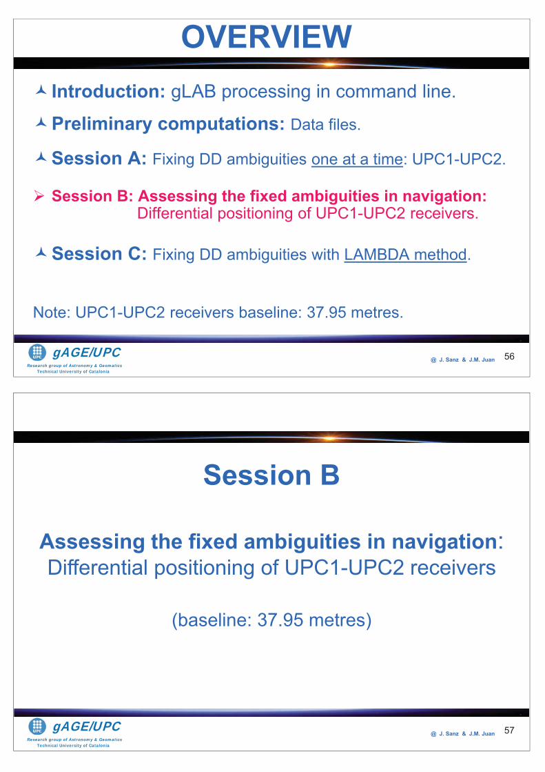
Research group of Astronomy & GeomaticsTechnical University of Catalonia
gAGE/UPC @ J. Sanz & J.M. Juan
Introduction: gLAB processing in command line.
Preliminary computations: Data files.
Session A: Fixing DD ambiguities one at a time: UPC1-UPC2.
Session B: Assessing the fixed ambiguities in navigation: Differential positioning of UPC1-UPC2 receivers.
Session C: Fixing DD ambiguities with LAMBDA method.
Note: UPC1-UPC2 receivers baseline: 37.95 metres.
OVERVIEW
56
Research group of Astronomy & GeomaticsTechnical University of Catalonia
gAGE/UPC @ J. Sanz & J.M. Juan 57
Session B
Assessing the fixed ambiguities in navigation: Differential positioning of UPC1-UPC2 receivers
(baseline: 37.95 metres)
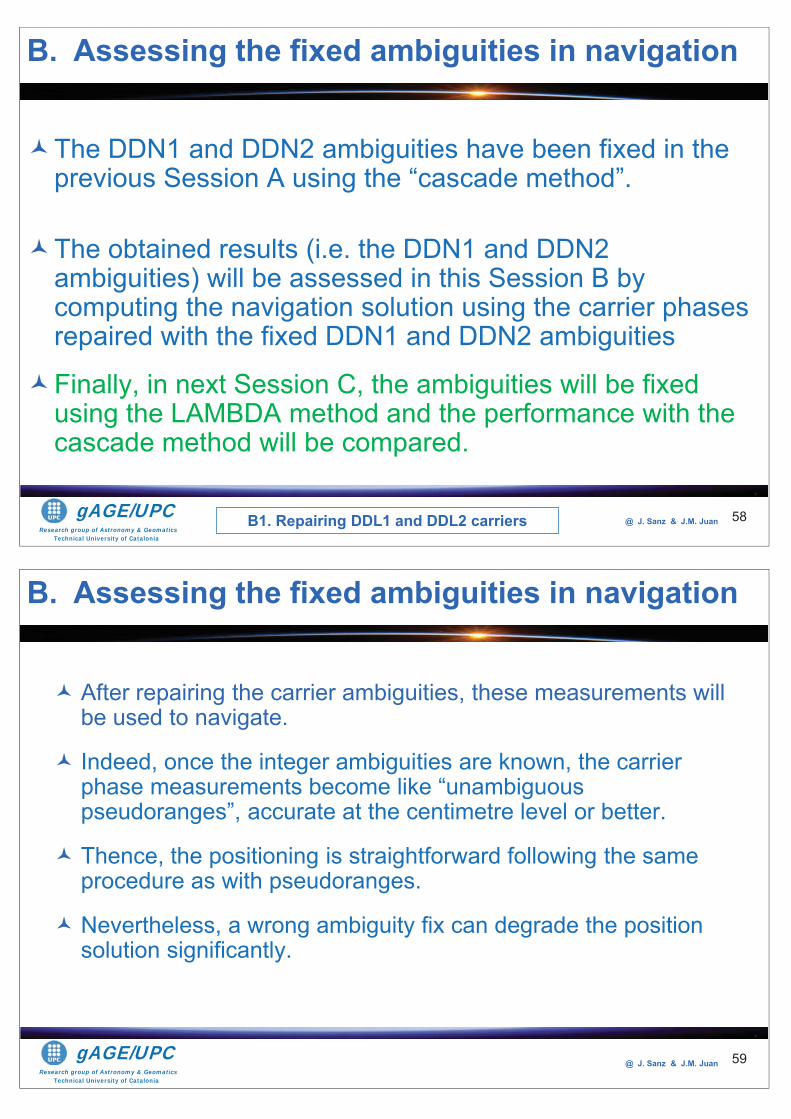
Research group of Astronomy & GeomaticsTechnical University of Catalonia
gAGE/UPC @ J. Sanz & J.M. Juan 58
The DDN1 and DDN2 ambiguities have been fixed in the previous Session A using the “cascade method”.
The obtained results (i.e. the DDN1 and DDN2 ambiguities) will be assessed in this Session B by computing the navigation solution using the carrier phases repaired with the fixed DDN1 and DDN2 ambiguities
Finally, in next Session C, the ambiguities will be fixed using the LAMBDA method and the performance with the cascade method will be compared.
B. Assessing the fixed ambiguities in navigation
B1. Repairing DDL1 and DDL2 carriers
Research group of Astronomy & GeomaticsTechnical University of Catalonia
gAGE/UPC @ J. Sanz & J.M. Juan 59
After repairing the carrier ambiguities, these measurements will be used to navigate.
Indeed, once the integer ambiguities are known, the carrier phase measurements become like “unambiguous pseudoranges”, accurate at the centimetre level or better.
Thence, the positioning is straightforward following the same procedure as with pseudoranges.
Nevertheless, a wrong ambiguity fix can degrade the position solution significantly.
B. Assessing the fixed ambiguities in navigation
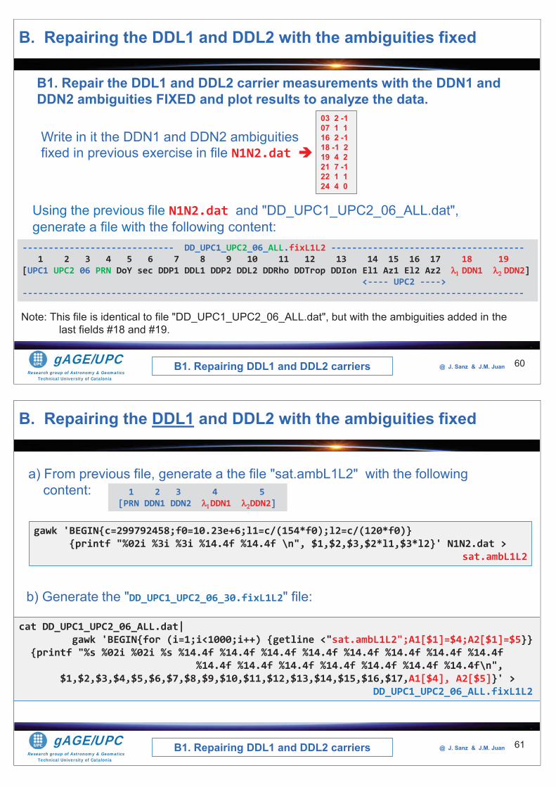
Research group of Astronomy & GeomaticsTechnical University of Catalonia
gAGE/UPC @ J. Sanz & J.M. Juan 60
B1. Repair the DDL1 and DDL2 carrier measurements with the DDN1 and DDN2 ambiguities FIXED and plot results to analyze the data.
03 2 -107 1 116 2 -118 -1 219 4 2 21 7 -122 1 124 4 0
Using the previous file N1N2.dat and "DD_UPC1_UPC2_06_ALL.dat",generate a file with the following content:
----------------------------- DD_UPC1_UPC2_06_ALL.fixL1L2 -------------------------------------1 2 3 4 5 6 7 8 9 10 11 12 13 14 15 16 17 18 19
[UPC1 UPC2 06 PRN DoY sec DDP1 DDL1 DDP2 DDL2 DDRho DDTrop DDIon El1 Az1 El2 Az2 DDN1 DDN2]<---- UPC2 ---->
------------------------------------------------------------------------------------------------
Note: This file is identical to file "DD_UPC1_UPC2_06_ALL.dat", but with the ambiguities added in the last fields #18 and #19.
B. Repairing the DDL1 and DDL2 with the ambiguities fixed
B1. Repairing DDL1 and DDL2 carriers
Write in it the DDN1 and DDN2 ambiguities fixed in previous exercise in file N1N2.dat
Research group of Astronomy & GeomaticsTechnical University of Catalonia
gAGE/UPC @ J. Sanz & J.M. Juan 61
gawk 'BEGIN{c=299792458;f0=10.23e+6;l1=c/(154*f0);l2=c/(120*f0)}{printf "%02i %3i %3i %14.4f %14.4f \n", $1,$2,$3,$2*l1,$3*l2}' N1N2.dat >
sat.ambL1L2
a) From previous file, generate a the file "sat.ambL1L2" with the following content:
cat DD_UPC1_UPC2_06_ALL.dat|gawk 'BEGIN{for (i=1;i<1000;i++) {getline <"sat.ambL1L2";A1[$1]=$4;A2[$1]=$5}}
{printf "%s %02i %02i %s %14.4f %14.4f %14.4f %14.4f %14.4f %14.4f %14.4f %14.4f %14.4f %14.4f %14.4f %14.4f %14.4f %14.4f %14.4f\n",
$1,$2,$3,$4,$5,$6,$7,$8,$9,$10,$11,$12,$13,$14,$15,$16,$17,A1[$4], A2[$5]}' > DD_UPC1_UPC2_06_ALL.fixL1L2
b) Generate the "DD_UPC1_UPC2_06_30.fixL1L2" file:
B1. Repairing DDL1 and DDL2 carriers
1 2 3 4 5[PRN DDN1 DDN2 DDN1 DDN2]
B. Repairing the DDL1 and DDL2 with the ambiguities fixed
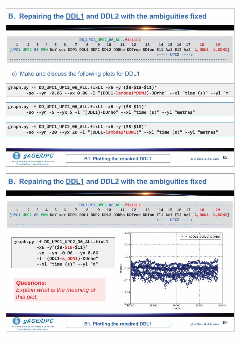
Research group of Astronomy & GeomaticsTechnical University of Catalonia
gAGE/UPC @ J. Sanz & J.M. Juan 62
graph.py -f DD_UPC1_UPC2_06_ALL.fixL1 -x6 -y'($8-$18-$11)' -so --yn -0.06 --yx 0.06 -l "(DDL1-lambda1*DDN1)-DDrho" --xl "time (s)" --yl "m"
c) Make and discuss the following plots for DDL1
graph.py -f DD_UPC1_UPC2_06_ALL.fixL1 -x6 -y'($8-$11)' -so --yn -5 --yx 5 -l "(DDL1)-DDrho" --xl "time (s)" --yl "metres"
graph.py -f DD_UPC1_UPC2_06_ALL.fixL1 -x6 -y'($8-$18)' -so --yn -20 --yx 20 -l "(DDL1-lambda1*DDN1)" --xl "time (s)" --yl "metres"
B. Repairing the DDL1 and DDL2 with the ambiguities fixed
B1. Plotting the repaired DDL1
----------------------------- DD_UPC1_UPC2_06_ALL.fixL1L2 -------------------------------------1 2 3 4 5 6 7 8 9 10 11 12 13 14 15 16 17 18 19
[UPC1 UPC2 06 PRN DoY sec DDP1 DDL1 DDP2 DDL2 DDRho DDTrop DDIon El1 Az1 El2 Az2 DDN1 DDN2]<---- UPC2 ---->
------------------------------------------------------------------------------------------------
Research group of Astronomy & GeomaticsTechnical University of Catalonia
gAGE/UPC @ J. Sanz & J.M. Juan 63
graph.py -f DD_UPC1_UPC2_06_ALL.fixL1 -x6 -y'($8-$18-$11)' -so --yn -0.06 --yx 0.06 -l "(DDL1- DDN1)-DDrho" --xl "time (s)" --yl "m"
Questions:Explain what is the meaning of this plot.
----------------------------- DD_UPC1_UPC2_06_ALL.fixL1L2 -------------------------------------1 2 3 4 5 6 7 8 9 10 11 12 13 14 15 16 17 18 19
[UPC1 UPC2 06 PRN DoY sec DDP1 DDL1 DDP2 DDL2 DDRho DDTrop DDIon El1 Az1 El2 Az2 DDN1 DDN2]<---- UPC2 ---->
------------------------------------------------------------------------------------------------
B. Repairing the DDL1 and DDL2 with the ambiguities fixed
B1. Plotting the repaired DDL1
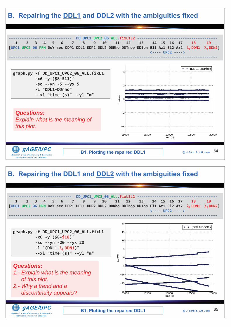
Research group of Astronomy & GeomaticsTechnical University of Catalonia
gAGE/UPC @ J. Sanz & J.M. Juan 64
graph.py -f DD_UPC1_UPC2_06_ALL.fixL1 -x6 -y'($8-$11)' -so --yn -5 --yx 5 -l "DDL1-DDrho" --xl "time (s)" --yl "m"
Questions:Explain what is the meaning of this plot.
----------------------------- DD_UPC1_UPC2_06_ALL.fixL1L2 -------------------------------------1 2 3 4 5 6 7 8 9 10 11 12 13 14 15 16 17 18 19
[UPC1 UPC2 06 PRN DoY sec DDP1 DDL1 DDP2 DDL2 DDRho DDTrop DDIon El1 Az1 El2 Az2 DDN1 DDN2]<---- UPC2 ---->
------------------------------------------------------------------------------------------------
B. Repairing the DDL1 and DDL2 with the ambiguities fixed
B1. Plotting the repaired DDL1
Research group of Astronomy & GeomaticsTechnical University of Catalonia
gAGE/UPC @ J. Sanz & J.M. Juan 65
graph.py -f DD_UPC1_UPC2_06_ALL.fixL1 -x6 -y'($8-$18)' -so --yn -20 --yx 20 -l "(DDL1- DDN1)" --xl "time (s)" --yl "m"
Questions:1.- Explain what is the meaning
of this plot.2.- Why a trend and a
discontinuity appears?
----------------------------- DD_UPC1_UPC2_06_ALL.fixL1L2 -------------------------------------1 2 3 4 5 6 7 8 9 10 11 12 13 14 15 16 17 18 19
[UPC1 UPC2 06 PRN DoY sec DDP1 DDL1 DDP2 DDL2 DDRho DDTrop DDIon El1 Az1 El2 Az2 DDN1 DDN2]<---- UPC2 ---->
------------------------------------------------------------------------------------------------
B. Repairing the DDL1 and DDL2 with the ambiguities fixed
B1. Plotting the repaired DDL1
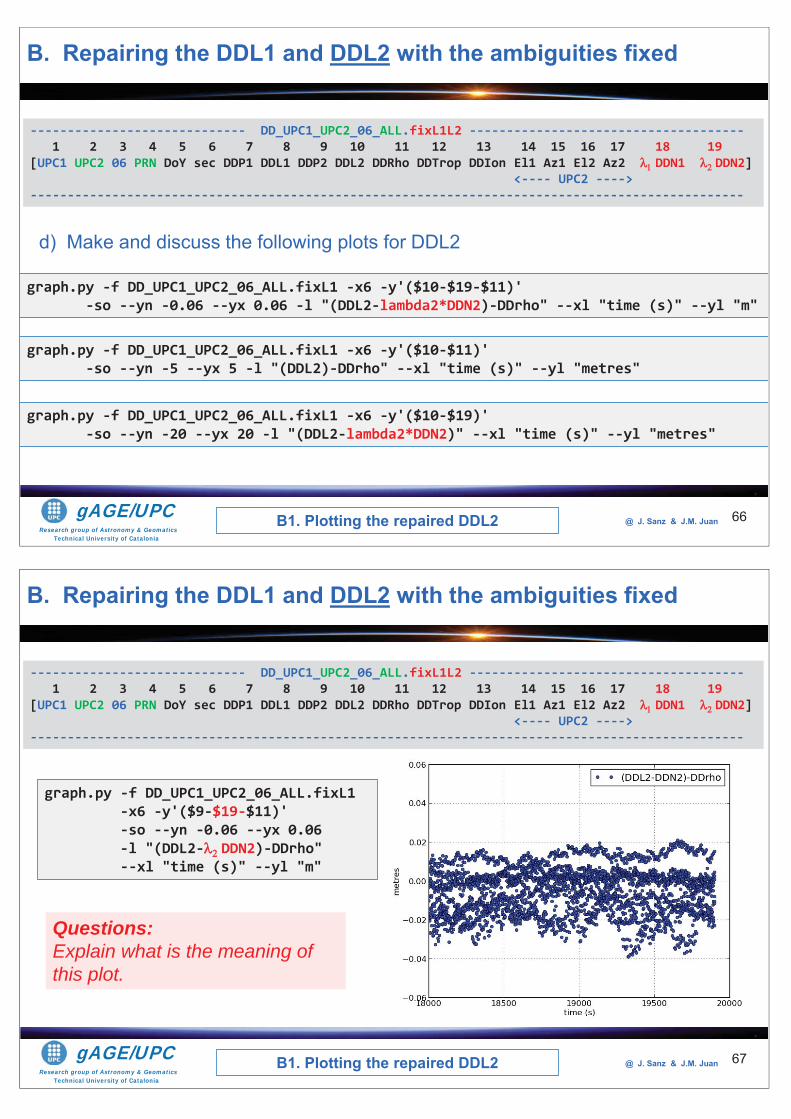
Research group of Astronomy & GeomaticsTechnical University of Catalonia
gAGE/UPC @ J. Sanz & J.M. Juan 66
graph.py -f DD_UPC1_UPC2_06_ALL.fixL1 -x6 -y'($10-$19-$11)' -so --yn -0.06 --yx 0.06 -l "(DDL2-lambda2*DDN2)-DDrho" --xl "time (s)" --yl "m"
d) Make and discuss the following plots for DDL2
graph.py -f DD_UPC1_UPC2_06_ALL.fixL1 -x6 -y'($10-$11)' -so --yn -5 --yx 5 -l "(DDL2)-DDrho" --xl "time (s)" --yl "metres"
graph.py -f DD_UPC1_UPC2_06_ALL.fixL1 -x6 -y'($10-$19)' -so --yn -20 --yx 20 -l "(DDL2-lambda2*DDN2)" --xl "time (s)" --yl "metres"
B. Repairing the DDL1 and DDL2 with the ambiguities fixed
B1. Plotting the repaired DDL2
----------------------------- DD_UPC1_UPC2_06_ALL.fixL1L2 -------------------------------------1 2 3 4 5 6 7 8 9 10 11 12 13 14 15 16 17 18 19
[UPC1 UPC2 06 PRN DoY sec DDP1 DDL1 DDP2 DDL2 DDRho DDTrop DDIon El1 Az1 El2 Az2 DDN1 DDN2]<---- UPC2 ---->
------------------------------------------------------------------------------------------------
Research group of Astronomy & GeomaticsTechnical University of Catalonia
gAGE/UPC @ J. Sanz & J.M. Juan 67
graph.py -f DD_UPC1_UPC2_06_ALL.fixL1 -x6 -y'($9-$19-$11)' -so --yn -0.06 --yx 0.06 -l "(DDL2- DDN2)-DDrho" --xl "time (s)" --yl "m"
Questions:Explain what is the meaning of this plot.
----------------------------- DD_UPC1_UPC2_06_ALL.fixL1L2 -------------------------------------1 2 3 4 5 6 7 8 9 10 11 12 13 14 15 16 17 18 19
[UPC1 UPC2 06 PRN DoY sec DDP1 DDL1 DDP2 DDL2 DDRho DDTrop DDIon El1 Az1 El2 Az2 DDN1 DDN2]<---- UPC2 ---->
------------------------------------------------------------------------------------------------
B. Repairing the DDL1 and DDL2 with the ambiguities fixed
B1. Plotting the repaired DDL2
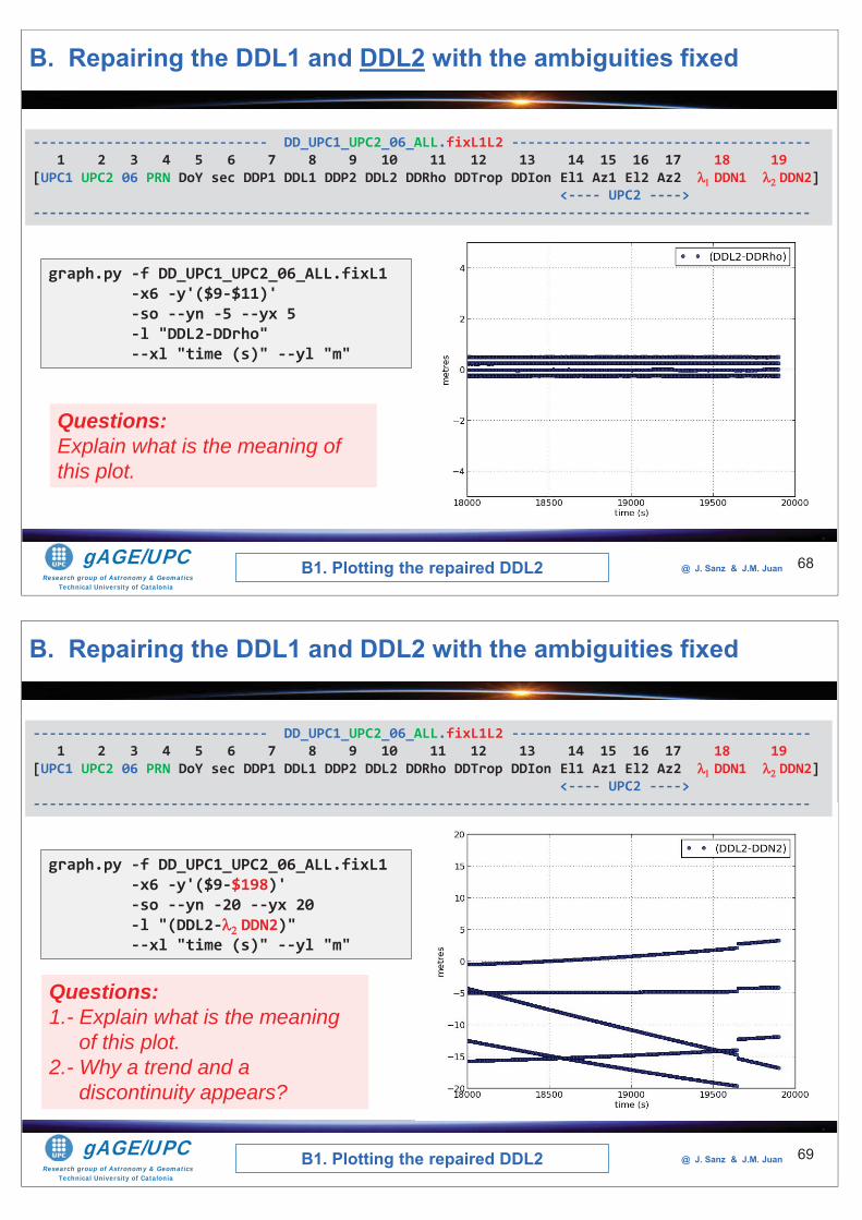
Research group of Astronomy & GeomaticsTechnical University of Catalonia
gAGE/UPC @ J. Sanz & J.M. Juan 68
graph.py -f DD_UPC1_UPC2_06_ALL.fixL1 -x6 -y'($9-$11)' -so --yn -5 --yx 5 -l "DDL2-DDrho" --xl "time (s)" --yl "m"
Questions:Explain what is the meaning of this plot.
----------------------------- DD_UPC1_UPC2_06_ALL.fixL1L2 -------------------------------------1 2 3 4 5 6 7 8 9 10 11 12 13 14 15 16 17 18 19
[UPC1 UPC2 06 PRN DoY sec DDP1 DDL1 DDP2 DDL2 DDRho DDTrop DDIon El1 Az1 El2 Az2 DDN1 DDN2]<---- UPC2 ---->
------------------------------------------------------------------------------------------------
B. Repairing the DDL1 and DDL2 with the ambiguities fixed
B1. Plotting the repaired DDL2
Research group of Astronomy & GeomaticsTechnical University of Catalonia
gAGE/UPC @ J. Sanz & J.M. Juan 69
graph.py -f DD_UPC1_UPC2_06_ALL.fixL1 -x6 -y'($9-$198)' -so --yn -20 --yx 20 -l "(DDL2- DDN2)" --xl "time (s)" --yl "m"
----------------------------- DD_UPC1_UPC2_06_ALL.fixL1L2 -------------------------------------1 2 3 4 5 6 7 8 9 10 11 12 13 14 15 16 17 18 19
[UPC1 UPC2 06 PRN DoY sec DDP1 DDL1 DDP2 DDL2 DDRho DDTrop DDIon El1 Az1 El2 Az2 DDN1 DDN2]<---- UPC2 ---->
------------------------------------------------------------------------------------------------
B. Repairing the DDL1 and DDL2 with the ambiguities fixed
B1. Plotting the repaired DDL2
Questions:1.- Explain what is the meaning
of this plot.2.- Why a trend and a
discontinuity appears?
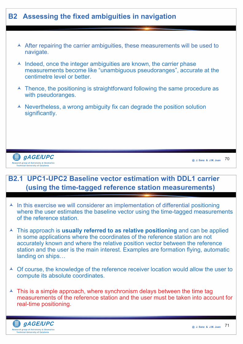
Research group of Astronomy & GeomaticsTechnical University of Catalonia
gAGE/UPC @ J. Sanz & J.M. Juan 70
After repairing the carrier ambiguities, these measurements will be used to navigate.
Indeed, once the integer ambiguities are known, the carrier phase measurements become like “unambiguous pseudoranges”, accurate at the centimetre level or better.
Thence, the positioning is straightforward following the same procedure as with pseudoranges.
Nevertheless, a wrong ambiguity fix can degrade the position solution significantly.
B2 Assessing the fixed ambiguities in navigation
Research group of Astronomy & GeomaticsTechnical University of Catalonia
gAGE/UPC @ J. Sanz & J.M. Juan 71
In this exercise we will considerer an implementation of differential positioning where the user estimates the baseline vector using the time-tagged measurements of the reference station.
This approach is usually referred to as relative positioning and can be applied in some applications where the coordinates of the reference station are not accurately known and where the relative position vector between the reference station and the user is the main interest. Examples are formation flying, automatic landing on ships…
Of course, the knowledge of the reference receiver location would allow the user to compute its absolute coordinates.
This is a simple approach, where synchronism delays between the time tag measurements of the reference station and the user must be taken into account for real-time positioning.
B2.1 UPC1-UPC2 Baseline vector estimation with DDL1 carrier(using the time-tagged reference station measurements)
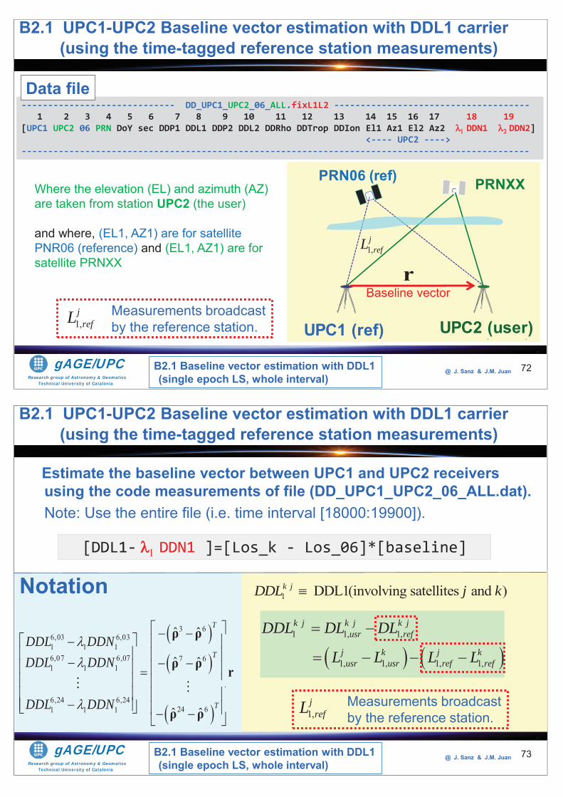
Research group of Astronomy & GeomaticsTechnical University of Catalonia
gAGE/UPC @ J. Sanz & J.M. Juan 72
Where the elevation (EL) and azimuth (AZ) are taken from station UPC2 (the user)
and where, (EL1, AZ1) are for satellite PNR06 (reference) and (EL1, AZ1) are for satellite PRNXX
B2.1 UPC1-UPC2 Baseline vector estimation with DDL1 carrier(using the time-tagged reference station measurements)
----------------------------- DD_UPC1_UPC2_06_ALL.fixL1L2 -------------------------------------1 2 3 4 5 6 7 8 9 10 11 12 13 14 15 16 17 18 19
[UPC1 UPC2 06 PRN DoY sec DDP1 DDL1 DDP2 DDL2 DDRho DDTrop DDIon El1 Az1 El2 Az2 DDN1 DDN2]<---- UPC2 ---->
------------------------------------------------------------------------------------------------
IND3 (user)IND2 (ref)
PRN06 (ref) PRNXX
UPC1 (ref) UPC2 (user)
Data file
Measurements broadcast by the reference station.1,
jrefL
1,jrefL
Baseline vectorr
B2.1 Baseline vector estimation with DDL1 (single epoch LS, whole interval)
Research group of Astronomy & GeomaticsTechnical University of Catalonia
gAGE/UPC @ J. Sanz & J.M. Juan 73
1 DDL1(involving satellites and )k jDDL j k
1 1, 1,
1, 1, 1, 1,
k j k j k jusr ref
j k j kusr usr ref ref
DDL DL DL
L L L L
1,jrefL Measurements broadcast
by the reference station.
[DDL1- DDN1 ]=[Los_k - Los_06]*[baseline]
3 66,03 6,031 1 16,07 6,07 7 61 1 1
6,24 6,2424 61 1 1
ˆ ˆ
ˆ ˆ
ˆ ˆ
T
T
T
DDL DDNDDL DDN
DDL DDN
ρ ρ
ρ ρ r
ρ ρ
Notation
Estimate the baseline vector between UPC1 and UPC2 receivers using the code measurements of file (DD_UPC1_UPC2_06_ALL.dat). Note: Use the entire file (i.e. time interval [18000:19900]).
B2.1 UPC1-UPC2 Baseline vector estimation with DDL1 carrier(using the time-tagged reference station measurements)
B2.1 Baseline vector estimation with DDL1 (single epoch LS, whole interval)
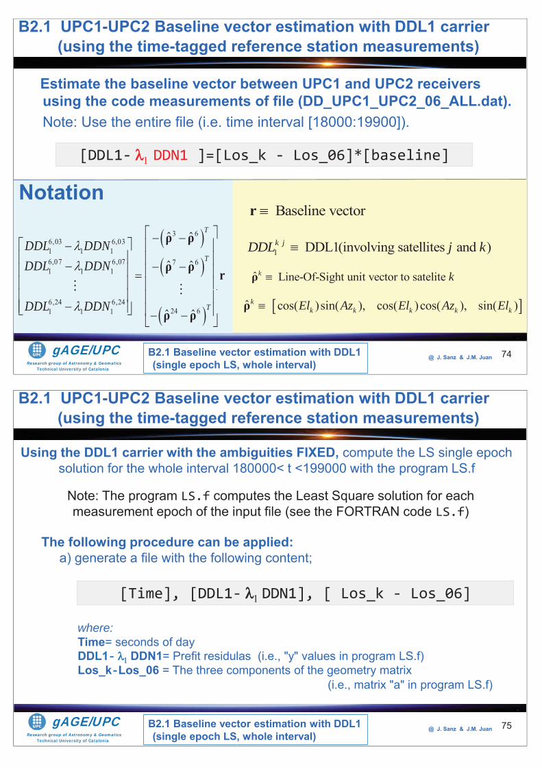
Research group of Astronomy & GeomaticsTechnical University of Catalonia
gAGE/UPC @ J. Sanz & J.M. Juan
Estimate the baseline vector between UPC1 and UPC2 receivers using the code measurements of file (DD_UPC1_UPC2_06_ALL.dat). Note: Use the entire file (i.e. time interval [18000:19900]).
74
[DDL1- DDN1 ]=[Los_k - Los_06]*[baseline]
3 66,03 6,031 1 16,07 6,07 7 61 1 1
6,24 6,2424 61 1 1
ˆ ˆ
ˆ ˆ
ˆ ˆ
T
T
T
DDL DDNDDL DDN
DDL DDN
ρ ρ
ρ ρ r
ρ ρ
1 DDL1(involving satellites and )k jDDL j k
ˆ Line-Of-Sight unit vector to satelite k kρ
ˆ cos( )sin( ), cos( )cos( ), sin( )kk k k k kEl Az El Az Elρ
Baseline vectorrNotation
B2.1 UPC1-UPC2 Baseline vector estimation with DDL1 carrier(using the time-tagged reference station measurements)
B2.1 Baseline vector estimation with DDL1 (single epoch LS, whole interval)
Research group of Astronomy & GeomaticsTechnical University of Catalonia
gAGE/UPC @ J. Sanz & J.M. Juan 75
Using the DDL1 carrier with the ambiguities FIXED, compute the LS single epoch solution for the whole interval 180000< t <199000 with the program LS.f
Note: The program LS.f computes the Least Square solution for eachmeasurement epoch of the input file (see the FORTRAN code LS.f)
The following procedure can be applied:a) generate a file with the following content;
[Time], [DDL1- DDN1], [ Los_k - Los_06]
where:Time= seconds of day DDL1- DDN1= Prefit residulas (i.e., "y" values in program LS.f)Los_k-Los_06 = The three components of the geometry matrix
(i.e., matrix "a" in program LS.f)
B2.1 Baseline vector estimation with DDL1 (single epoch LS, whole interval)
B2.1 UPC1-UPC2 Baseline vector estimation with DDL1 carrier(using the time-tagged reference station measurements)
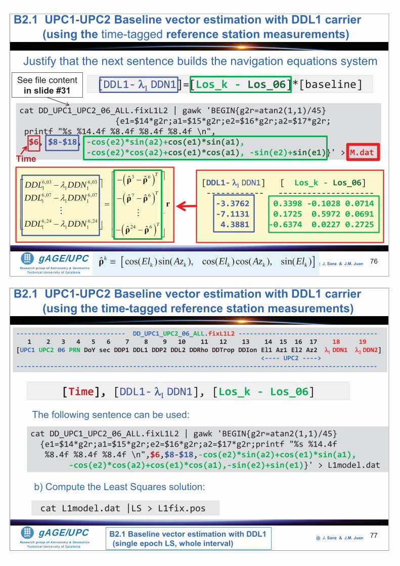
Research group of Astronomy & GeomaticsTechnical University of Catalonia
gAGE/UPC @ J. Sanz & J.M. Juan 76
cat DD_UPC1_UPC2_06_ALL.fixL1L2 | gawk 'BEGIN{g2r=atan2(1,1)/45} {e1=$14*g2r;a1=$15*g2r;e2=$16*g2r;a2=$17*g2r;
printf "%s %14.4f %8.4f %8.4f %8.4f \n",$6, $8-$18, -cos(e2)*sin(a2)+cos(e1)*sin(a1),
-cos(e2)*cos(a2)+cos(e1)*cos(a1), -sin(e2)+sin(e1)}' > M.dat
Justify that the next sentence builds the navigation equations system
[DDL1- DDN1]=[Los_k - Los_06]*[baseline]
[DDL1- DDN1] [ Los_k - Los_06] ------------ ---------------------3.3762 0.3398 -0.1028 0.0714-7.1131 0.1725 0.5972 0.0691 4.3881 -0.6374 0.0227 0.2725
3 66,03 6,031 1 16,07 6,07 7 61 1 1
6,24 6,2424 61 1 1
ˆ ˆ
ˆ ˆ
ˆ ˆ
T
T
T
DDL DDNDDL DDN
DDL DDN
ρ ρ
ρ ρ r
ρ ρ
ˆ cos( )sin( ), cos( )cos( ), sin( )kk k k k kEl Az El Az Elρ
B2.1 UPC1-UPC2 Baseline vector estimation with DDL1 carrier(using the time-tagged reference station measurements)
See file content in slide #31
Time
Research group of Astronomy & GeomaticsTechnical University of Catalonia
gAGE/UPC @ J. Sanz & J.M. Juan 77
The following sentence can be used:
cat DD_UPC1_UPC2_06_ALL.fixL1L2 | gawk 'BEGIN{g2r=atan2(1,1)/45} {e1=$14*g2r;a1=$15*g2r;e2=$16*g2r;a2=$17*g2r;printf "%s %14.4f%8.4f %8.4f %8.4f \n",$6,$8-$18,-cos(e2)*sin(a2)+cos(e1)*sin(a1),
-cos(e2)*cos(a2)+cos(e1)*cos(a1),-sin(e2)+sin(e1)}' > L1model.dat
[Time], [DDL1- DDN1], [Los_k - Los_06]
b) Compute the Least Squares solution:
cat L1model.dat |LS > L1fix.pos
B2.1 UPC1-UPC2 Baseline vector estimation with DDL1 carrier(using the time-tagged reference station measurements)
B2.1 Baseline vector estimation with DDL1 (single epoch LS, whole interval)
----------------------------- DD_UPC1_UPC2_06_ALL.fixL1L2 -------------------------------------1 2 3 4 5 6 7 8 9 10 11 12 13 14 15 16 17 18 19
[UPC1 UPC2 06 PRN DoY sec DDP1 DDL1 DDP2 DDL2 DDRho DDTrop DDIon El1 Az1 El2 Az2 DDN1 DDN2]<---- UPC2 ---->
------------------------------------------------------------------------------------------------
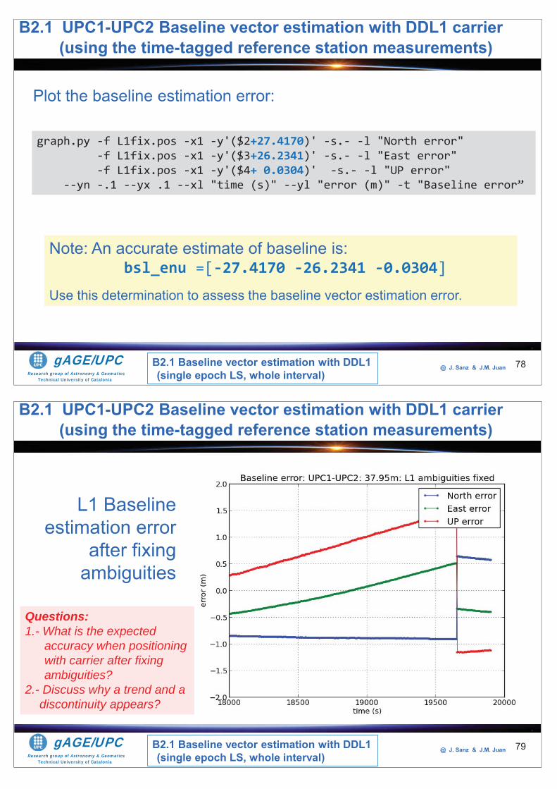
Research group of Astronomy & GeomaticsTechnical University of Catalonia
gAGE/UPC @ J. Sanz & J.M. Juan 78
Plot the baseline estimation error:
graph.py -f L1fix.pos -x1 -y'($2+27.4170)' -s.- -l "North error" -f L1fix.pos -x1 -y'($3+26.2341)' -s.- -l "East error" -f L1fix.pos -x1 -y'($4+ 0.0304)' -s.- -l "UP error"
--yn -.1 --yx .1 --xl "time (s)" --yl "error (m)" -t "Baseline error”
Note: An accurate estimate of baseline is:bsl_enu =[-27.4170 -26.2341 -0.0304]
Use this determination to assess the baseline vector estimation error.
B2.1 Baseline vector estimation with DDL1 (single epoch LS, whole interval)
B2.1 UPC1-UPC2 Baseline vector estimation with DDL1 carrier(using the time-tagged reference station measurements)
Research group of Astronomy & GeomaticsTechnical University of Catalonia
gAGE/UPC @ J. Sanz & J.M. Juan 79
L1 Baseline estimation error
after fixing ambiguities
B2.1 UPC1-UPC2 Baseline vector estimation with DDL1 carrier(using the time-tagged reference station measurements)
B2.1 Baseline vector estimation with DDL1 (single epoch LS, whole interval)
Questions:1.- What is the expected
accuracy when positioning with carrier after fixing ambiguities?
2.- Discuss why a trend and a discontinuity appears?
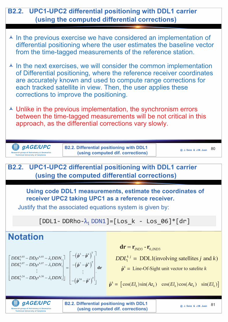
Research group of Astronomy & GeomaticsTechnical University of Catalonia
gAGE/UPC @ J. Sanz & J.M. Juan 80
In the previous exercise we have considered an implementation of differential positioning where the user estimates the baseline vector from the time-tagged measurements of the reference station.
In the next exercises, we will consider the common implementation of Differential positioning, where the reference receiver coordinates are accurately known and used to compute range corrections for each tracked satellite in view. Then, the user applies these corrections to improve the positioning.
Unlike in the previous implementation, the synchronism errors between the time-tagged measurements will be not critical in this approach, as the differential corrections vary slowly.
B2.2. UPC1-UPC2 differential positioning with DDL1 carrier(using the computed differential corrections)
B2.2. Differential positioning with DDL1 (using computed dif. corrections)
Research group of Astronomy & GeomaticsTechnical University of Catalonia
gAGE/UPC @ J. Sanz & J.M. Juan
Using code DDL1 measurements, estimate the coordinates of receiver UPC2 taking UPC1 as a reference receiver.
Justify that the associated equations system is given by:
81
1 DDL1(involving satellites and )k jDDL j kˆ Line-Of-Sight unit vector to satelite k kρ
ˆ cos( )sin( ) cos( )cos( ) sin( )kk k k k kEl Az El Az Elρ
3 0, 3-IND INDdr r rNotation
[DDL1- DDRho- DDN1]=[Los_k - Los_06]*[dr]
3 66,03 6,031 1 16,07 6,07 7 61 1 1
6,24 6,3024 61 1 1
ˆ ˆ
ˆ ˆ
ˆ ˆ
T
T
T
DDL DD DDNDDL DD DDN
DDL DD DDN
ρ ρ
ρ ρ dr
ρ ρ
B2.2. Differential positioning with DDL1 (using computed dif. corrections)
B2.2. UPC1-UPC2 differential positioning with DDL1 carrier(using the computed differential corrections)
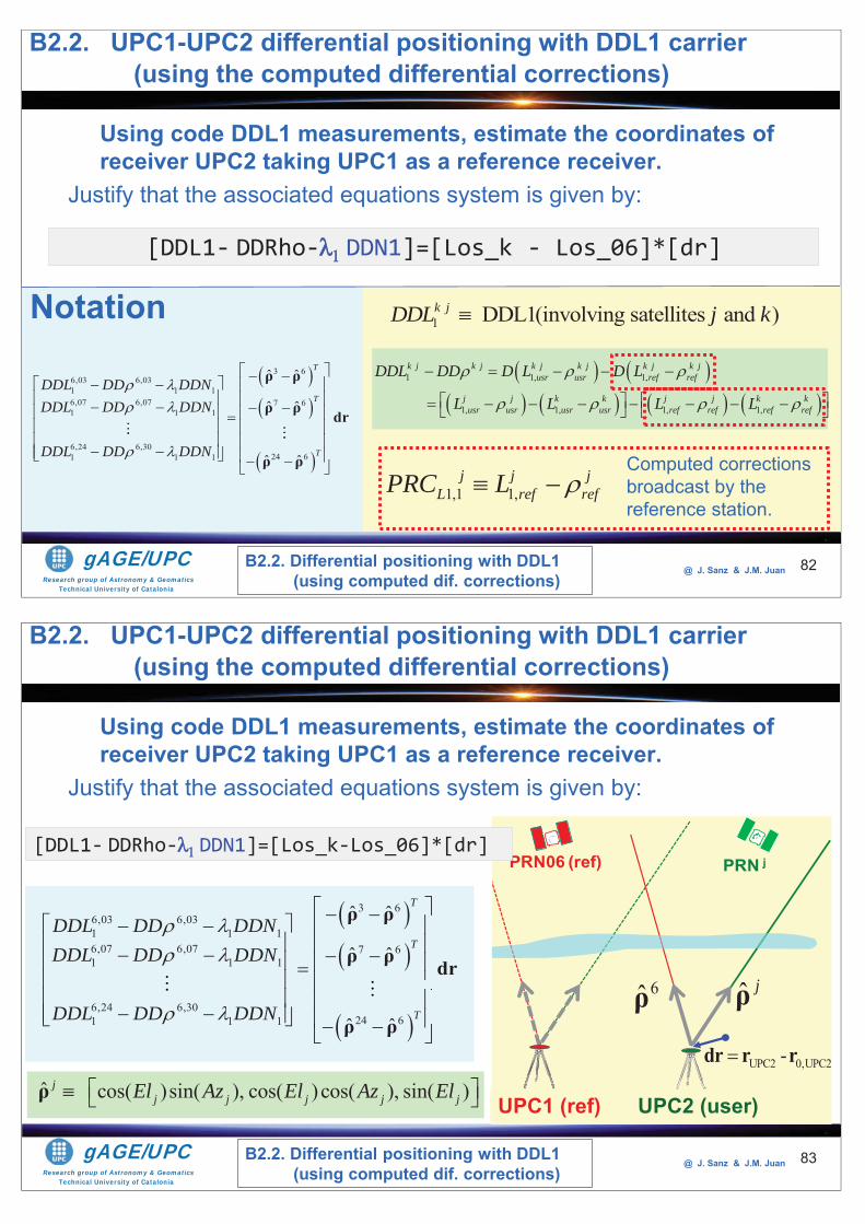
Research group of Astronomy & GeomaticsTechnical University of Catalonia
gAGE/UPC @ J. Sanz & J.M. Juan
Using code DDL1 measurements, estimate the coordinates of receiver UPC2 taking UPC1 as a reference receiver.
Justify that the associated equations system is given by:
82
[DDL1- DDRho- DDN1]=[Los_k - Los_06]*[dr]
Notation
1,1 1,j j j
L ref refPRC LComputed corrections broadcast by the reference station.
3 66,03 6,031 1 16,07 6,07 7 61 1 1
6,24 6,3024 61 1 1
ˆ ˆ
ˆ ˆ
ˆ ˆ
T
T
T
DDL DD DDNDDL DD DDN
DDL DD DDN
ρ ρ
ρ ρ dr
ρ ρ
1 1, 1,
1, 1, 1, 1,
k j k j k j k j k j k jusr usr ref ref
j j k k j j k kusr usr usr usr ref ref ref ref
DDL DD D L D L
L L L L
1 DDL1(involving satellites and )k jDDL j k
B2.2. Differential positioning with DDL1 (using computed dif. corrections)
B2.2. UPC1-UPC2 differential positioning with DDL1 carrier(using the computed differential corrections)
Research group of Astronomy & GeomaticsTechnical University of Catalonia
gAGE/UPC @ J. Sanz & J.M. Juan
IND3 (user)IND2 (ref)
PRN06 (ref) PRN j
83
[DDL1- DDRho- DDN1]=[Los_k-Los_06]*[dr]
6ρ ˆ jρ
UPC2 0,UPC2-dr r rˆ cos( )sin( ), cos( )cos( ), sin( )j
j j j j jEl Az El Az Elρ
3 66,03 6,031 1 16,07 6,07 7 61 1 1
6,24 6,3024 61 1 1
ˆ ˆ
ˆ ˆ
ˆ ˆ
T
T
T
DDL DD DDNDDL DD DDN
DDL DD DDN
ρ ρ
ρ ρ dr
ρ ρ
UPC1 (ref) UPC2 (user)
B2.2. Differential positioning with DDL1 (using computed dif. corrections)
B2.2. UPC1-UPC2 differential positioning with DDL1 carrier(using the computed differential corrections)
Using code DDL1 measurements, estimate the coordinates of receiver UPC2 taking UPC1 as a reference receiver.
Justify that the associated equations system is given by:
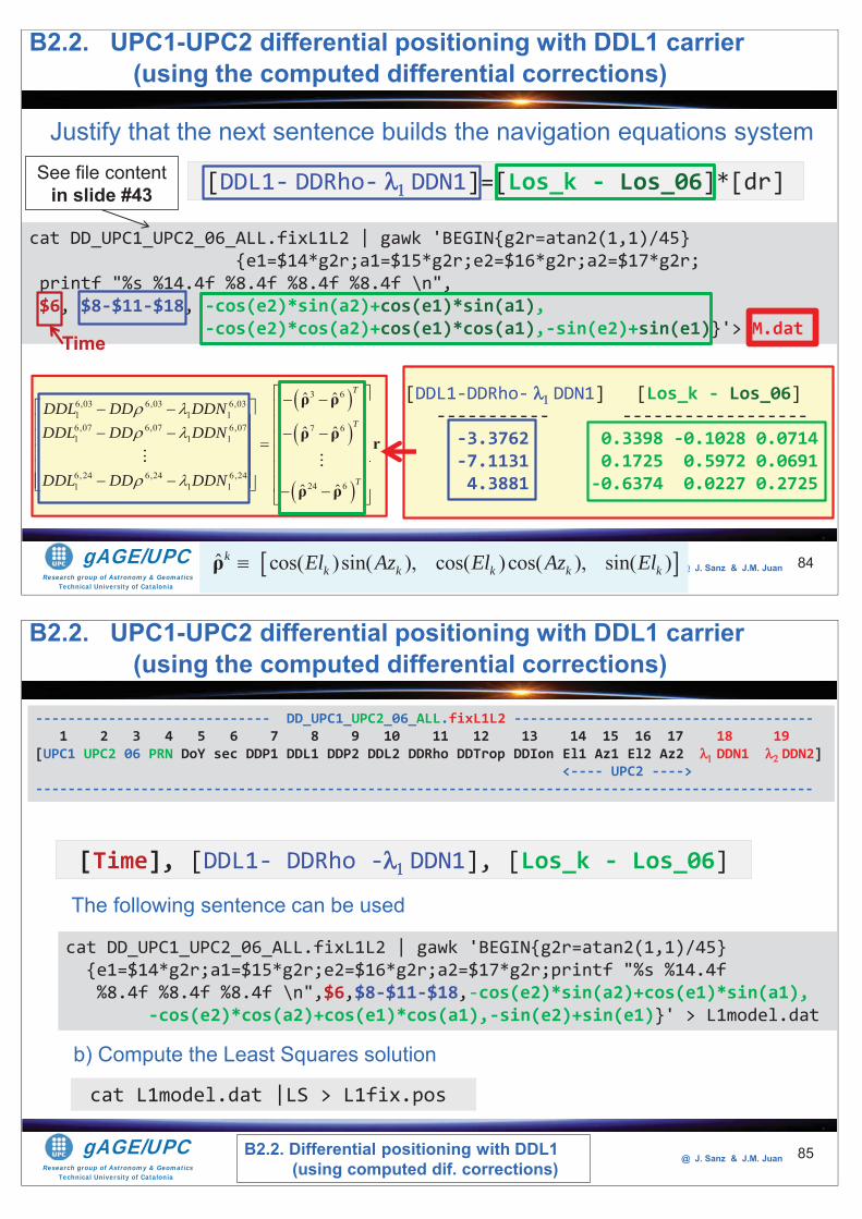
Research group of Astronomy & GeomaticsTechnical University of Catalonia
gAGE/UPC @ J. Sanz & J.M. Juan 84
cat DD_UPC1_UPC2_06_ALL.fixL1L2 | gawk 'BEGIN{g2r=atan2(1,1)/45} {e1=$14*g2r;a1=$15*g2r;e2=$16*g2r;a2=$17*g2r;
printf "%s %14.4f %8.4f %8.4f %8.4f \n",$6, $8-$11-$18, -cos(e2)*sin(a2)+cos(e1)*sin(a1),
-cos(e2)*cos(a2)+cos(e1)*cos(a1),-sin(e2)+sin(e1)}'> M.dat
Justify that the next sentence builds the navigation equations system
[DDL1- DDRho- DDN1]=[Los_k - Los_06]*[dr]
[DDL1-DDRho- DDN1] [Los_k - Los_06] ----------- -------------------3.3762 0.3398 -0.1028 0.0714-7.1131 0.1725 0.5972 0.0691 4.3881 -0.6374 0.0227 0.2725
3 66,03 6,03 6,031 1 16,07 6,07 6,07 7 61 1 1
6,24 6,24 6,2424 61 1 1
ˆ ˆ
ˆ ˆ
ˆ ˆ
T
T
T
DDL DD DDNDDL DD DDN
DDL DD DDN
ρ ρ
ρ ρ r
ρ ρ
ˆ cos( )sin( ), cos( )cos( ), sin( )kk k k k kEl Az El Az Elρ
See file content in slide #43
Time
B2.2. UPC1-UPC2 differential positioning with DDL1 carrier(using the computed differential corrections)
Research group of Astronomy & GeomaticsTechnical University of Catalonia
gAGE/UPC @ J. Sanz & J.M. Juan 85
The following sentence can be used
cat DD_UPC1_UPC2_06_ALL.fixL1L2 | gawk 'BEGIN{g2r=atan2(1,1)/45} {e1=$14*g2r;a1=$15*g2r;e2=$16*g2r;a2=$17*g2r;printf "%s %14.4f%8.4f %8.4f %8.4f \n",$6,$8-$11-$18,-cos(e2)*sin(a2)+cos(e1)*sin(a1),
-cos(e2)*cos(a2)+cos(e1)*cos(a1),-sin(e2)+sin(e1)}' > L1model.dat
[Time], [DDL1- DDRho - DDN1], [Los_k - Los_06]
b) Compute the Least Squares solution
cat L1model.dat |LS > L1fix.pos
----------------------------- DD_UPC1_UPC2_06_ALL.fixL1L2 -------------------------------------1 2 3 4 5 6 7 8 9 10 11 12 13 14 15 16 17 18 19
[UPC1 UPC2 06 PRN DoY sec DDP1 DDL1 DDP2 DDL2 DDRho DDTrop DDIon El1 Az1 El2 Az2 DDN1 DDN2]<---- UPC2 ---->
------------------------------------------------------------------------------------------------
B2.2. Differential positioning with DDL1 (using computed dif. corrections)
B2.2. UPC1-UPC2 differential positioning with DDL1 carrier(using the computed differential corrections)
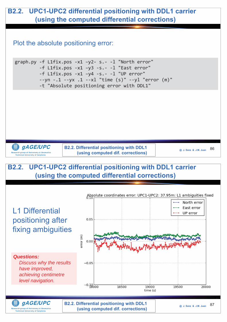
Research group of Astronomy & GeomaticsTechnical University of Catalonia
gAGE/UPC @ J. Sanz & J.M. Juan 86
Plot the absolute positioning error:
graph.py -f L1fix.pos -x1 –y2- s.- -l "North error" -f L1fix.pos -x1 –y3 -s.- -l "East error" -f L1fix.pos -x1 –y4 -s.- -l "UP error" --yn -.1 --yx .1 --xl "time (s)" --yl "error (m)" -t "Absolute positioning error with DDL1"
B2.2. Differential positioning with DDL1 (using computed dif. corrections)
B2.2. UPC1-UPC2 differential positioning with DDL1 carrier(using the computed differential corrections)
Research group of Astronomy & GeomaticsTechnical University of Catalonia
gAGE/UPC @ J. Sanz & J.M. Juan 87
L1 Differential positioning after fixing ambiguities
Questions:Discuss why the results have improved, achieving centimetre level navigation.
B2.2. Differential positioning with DDL1 (using computed dif. corrections)
B2.2. UPC1-UPC2 differential positioning with DDL1 carrier(using the computed differential corrections)
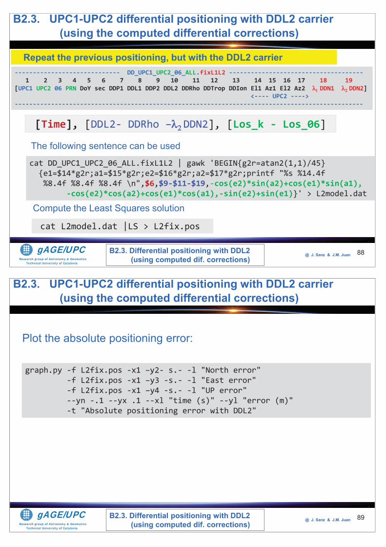
Research group of Astronomy & GeomaticsTechnical University of Catalonia
gAGE/UPC @ J. Sanz & J.M. Juan 88
The following sentence can be used
cat DD_UPC1_UPC2_06_ALL.fixL1L2 | gawk 'BEGIN{g2r=atan2(1,1)/45} {e1=$14*g2r;a1=$15*g2r;e2=$16*g2r;a2=$17*g2r;printf "%s %14.4f%8.4f %8.4f %8.4f \n",$6,$9-$11-$19,-cos(e2)*sin(a2)+cos(e1)*sin(a1),
-cos(e2)*cos(a2)+cos(e1)*cos(a1),-sin(e2)+sin(e1)}' > L2model.dat
[Time], [DDL2- DDRho – DDN2], [Los_k - Los_06]
Compute the Least Squares solution
cat L2model.dat |LS > L2fix.pos
----------------------------- DD_UPC1_UPC2_06_ALL.fixL1L2 -------------------------------------1 2 3 4 5 6 7 8 9 10 11 12 13 14 15 16 17 18 19
[UPC1 UPC2 06 PRN DoY sec DDP1 DDL1 DDP2 DDL2 DDRho DDTrop DDIon El1 Az1 El2 Az2 DDN1 DDN2]<---- UPC2 ---->
------------------------------------------------------------------------------------------------
B2.3. Differential positioning with DDL2 (using computed dif. corrections)
B2.3. UPC1-UPC2 differential positioning with DDL2 carrier(using the computed differential corrections)
Repeat the previous positioning, but with the DDL2 carrier
Research group of Astronomy & GeomaticsTechnical University of Catalonia
gAGE/UPC @ J. Sanz & J.M. Juan 89
Plot the absolute positioning error:
graph.py -f L2fix.pos -x1 –y2- s.- -l "North error" -f L2fix.pos -x1 –y3 -s.- -l "East error" -f L2fix.pos -x1 –y4 -s.- -l "UP error" --yn -.1 --yx .1 --xl "time (s)" --yl "error (m)" -t "Absolute positioning error with DDL2"
B2.3. Differential positioning with DDL2 (using computed dif. corrections)
B2.3. UPC1-UPC2 differential positioning with DDL2 carrier(using the computed differential corrections)
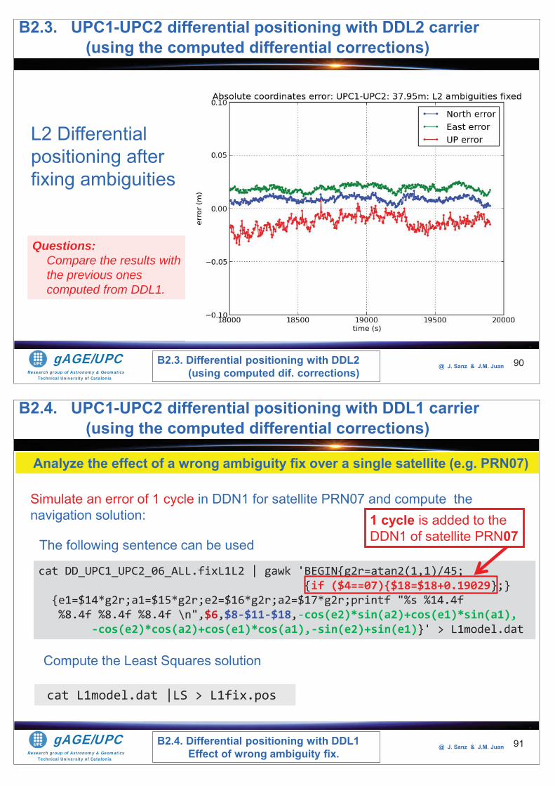
Research group of Astronomy & GeomaticsTechnical University of Catalonia
gAGE/UPC @ J. Sanz & J.M. Juan 90
L2 Differential positioning after fixing ambiguities
Questions:Compare the results with the previous ones computed from DDL1.
B2.3. Differential positioning with DDL2 (using computed dif. corrections)
B2.3. UPC1-UPC2 differential positioning with DDL2 carrier(using the computed differential corrections)
Research group of Astronomy & GeomaticsTechnical University of Catalonia
gAGE/UPC @ J. Sanz & J.M. Juan 91
The following sentence can be used
cat DD_UPC1_UPC2_06_ALL.fixL1L2 | gawk 'BEGIN{g2r=atan2(1,1)/45; {if ($4==07){$18=$18+0.19029};}
{e1=$14*g2r;a1=$15*g2r;e2=$16*g2r;a2=$17*g2r;printf "%s %14.4f%8.4f %8.4f %8.4f \n",$6,$8-$11-$18,-cos(e2)*sin(a2)+cos(e1)*sin(a1),
-cos(e2)*cos(a2)+cos(e1)*cos(a1),-sin(e2)+sin(e1)}' > L1model.dat
Compute the Least Squares solution
cat L1model.dat |LS > L1fix.pos
B2.4. Differential positioning with DDL1 Effect of wrong ambiguity fix.
B2.4. UPC1-UPC2 differential positioning with DDL1 carrier(using the computed differential corrections)
Analyze the effect of a wrong ambiguity fix over a single satellite (e.g. PRN07)
Simulate an error of 1 cycle in DDN1 for satellite PRN07 and compute the navigation solution: 1 cycle is added to the
DDN1 of satellite PRN07
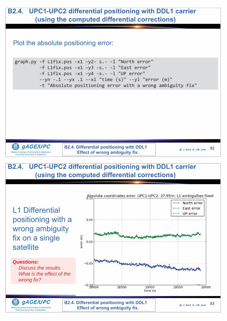
Research group of Astronomy & GeomaticsTechnical University of Catalonia
gAGE/UPC @ J. Sanz & J.M. Juan 92
Plot the absolute positioning error:
graph.py -f L1fix.pos -x1 –y2- s.- -l "North error" -f L1fix.pos -x1 –y3 -s.- -l "East error" -f L1fix.pos -x1 –y4 -s.- -l "UP error" --yn -.1 --yx .1 --xl "time (s)" --yl "error (m)" -t "Absolute positioning error with a wrong ambiguity fix"
B2.4. Differential positioning with DDL1 Effect of wrong ambiguity fix.
B2.4. UPC1-UPC2 differential positioning with DDL1 carrier(using the computed differential corrections)
Research group of Astronomy & GeomaticsTechnical University of Catalonia
gAGE/UPC @ J. Sanz & J.M. Juan 93
L1 Differential positioning with a wrong ambiguity fix on a single satellite
Questions:Discuss the results. What is the effect of the wrong fix?
B2.4. Differential positioning with DDL1 Effect of wrong ambiguity fix.
B2.4. UPC1-UPC2 differential positioning with DDL1 carrier(using the computed differential corrections)
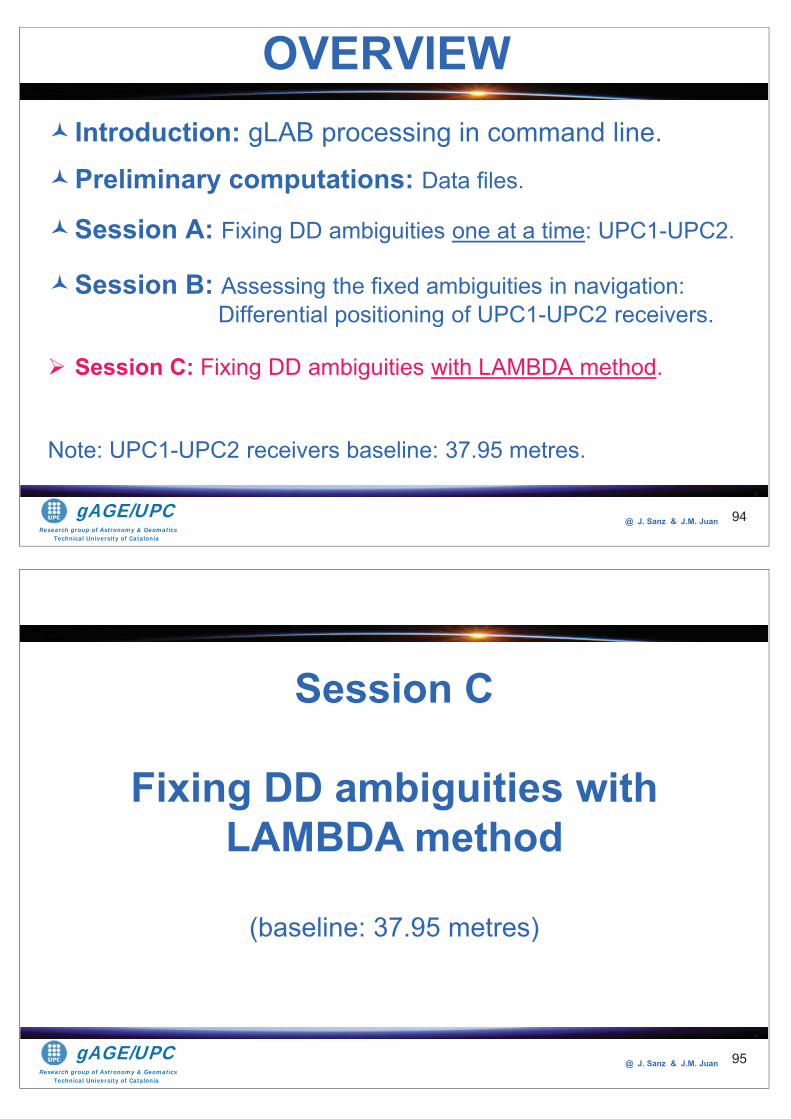
Research group of Astronomy & GeomaticsTechnical University of Catalonia
gAGE/UPC @ J. Sanz & J.M. Juan
Introduction: gLAB processing in command line.
Preliminary computations: Data files.
Session A: Fixing DD ambiguities one at a time: UPC1-UPC2.
Session B: Assessing the fixed ambiguities in navigation: Differential positioning of UPC1-UPC2 receivers.
Session C: Fixing DD ambiguities with LAMBDA method.
Note: UPC1-UPC2 receivers baseline: 37.95 metres.
OVERVIEW
94
Research group of Astronomy & GeomaticsTechnical University of Catalonia
gAGE/UPC @ J. Sanz & J.M. Juan 95
Session C
Fixing DD ambiguities with LAMBDA method
(baseline: 37.95 metres)
Research group of Astronomy & GeomaticsTechnical University of Catalonia
gAGE/UPC @ J. Sanz & J.M. Juan 96
Apply the LAMBDA method to fix the ambiguities.
Consider only the two epochs: t1=18000 and t2=18015.
Note: To avoid the synchronization issues, consider the Differential Positioning using the computed differential corrections, instead of the time-tagged measurements.
That is, we are going to solve the following navigation equations systems:
1. Navigating with L1 carrier, to fix DDN1:[DDL1-DDRho]=[Los_k-Los_06]*dr + [ A ]*[ *DDN1]
2. Navigating with L2 carrier, to fix DDN2:
[DDL2-DDRho]=[Los_k-Los_06]*dr + [ A ]*[ *DDN2]
C Fixing the DDN1 and DDN2 ambiguities with LAMBDA Method
C. Fixing DDN1 and DDN2 ambiguities with LAMBDA
gAG
E/U
PC re
sear
ch g
roup
of A
stro
nom
y an
d G
eom
atic
s
gAGE
Master of Science in GNSS @ J. Sanz & J.M. Juan97
Consider again the previous problem of estimating , a 3-vector of real numbers , and a (K-1)-vector of integers, which are solution of
rN
y G r AN νThe solution comprises the following steps:
1. Obtain the float solution and its covariance matrix:
2. Find the integer vector N which minimizes the cost function
a) Decorrelation: Using the Z transform, the ambiguity search space is re-parametrized to decorrelate the float ambiguities.
b) Integer ambiguities estimation (e.g. by rounding or by using sequential conditional least-squares adjustment, together with a discrete search strategy).
c) Using the Z-1 transform, the ambiguities are transformed to the original ambiguity space.
3. Obtain the ‘fixed’ solution r, from the fixed ambiguities N.
ˆ;ˆ
rN
ˆ ˆˆ ,
ˆ ˆˆ ,
r r N
r N N
P P
P P
1ˆ ˆN NW P
ˆ
2
ˆˆ ˆ ˆ( )
Tc
NNW
N N N N N W N N
y AN G r ν
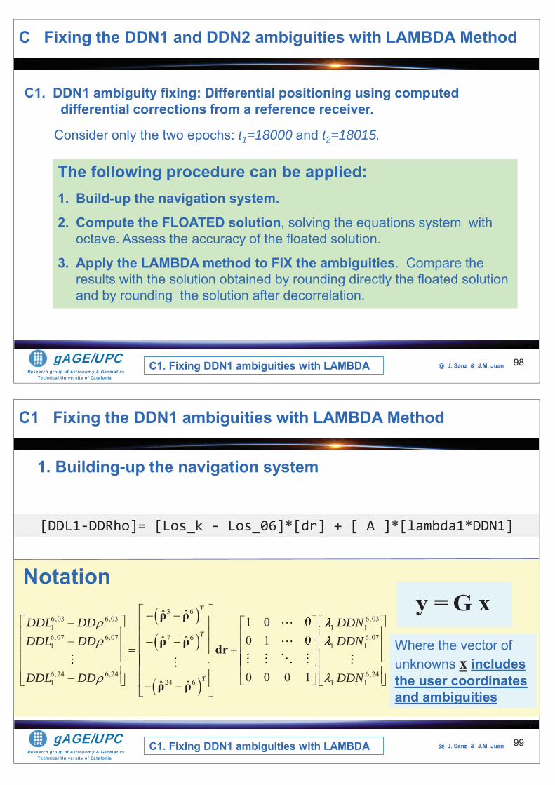
Research group of Astronomy & GeomaticsTechnical University of Catalonia
gAGE/UPC @ J. Sanz & J.M. Juan 98
C1. DDN1 ambiguity fixing: Differential positioning using computed differential corrections from a reference receiver.
Consider only the two epochs: t1=18000 and t2=18015.
The following procedure can be applied:1. Build-up the navigation system.
2. Compute the FLOATED solution, solving the equations system with octave. Assess the accuracy of the floated solution.
3. Apply the LAMBDA method to FIX the ambiguities. Compare the results with the solution obtained by rounding directly the floated solution and by rounding the solution after decorrelation.
C1. Fixing DDN1 ambiguities with LAMBDA
C Fixing the DDN1 and DDN2 ambiguities with LAMBDA Method
Research group of Astronomy & GeomaticsTechnical University of Catalonia
gAGE/UPC @ J. Sanz & J.M. Juan
1. Building-up the navigation system
99
[DDL1-DDRho]= [Los_k - Los_06]*[dr] + [ A ]*[lambda1*DDN1]
3 66,03 6,03 6,031 1 16,07 6,07 6,077 61 1 1
6,24 6,24 6,2424 61 1 1
ˆ ˆ 1 0 00 1 0ˆ ˆ
0 0 0 1ˆ ˆ
T
T
T
DDL DD DDNDDL DD DDN
DDL DD DDN
ρ ρ
ρ ρ dr
ρ ρ
1110 111
11110
Notation
Where the vector of unknowns x includes the user coordinates and ambiguities
y =G x
C1 Fixing the DDN1 ambiguities with LAMBDA Method
C1. Fixing DDN1 ambiguities with LAMBDA
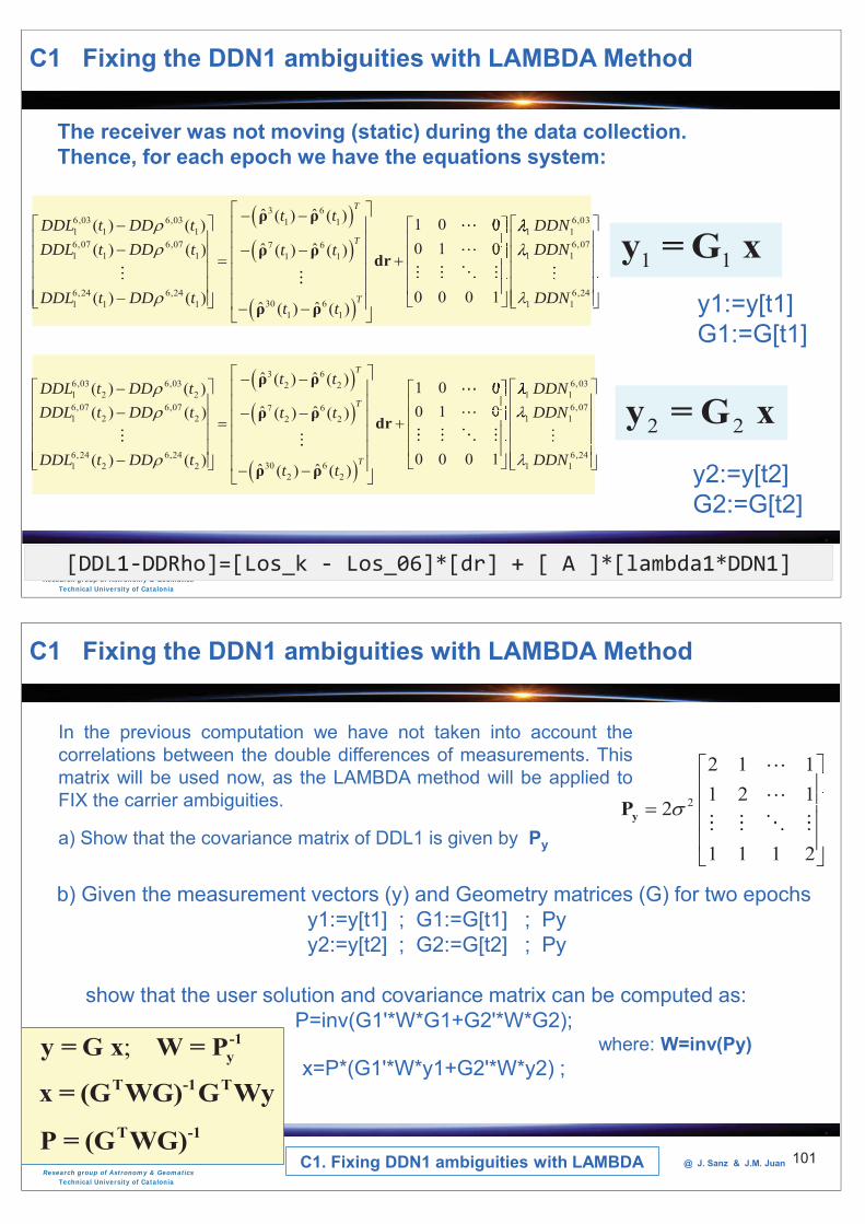
Research group of Astronomy & GeomaticsTechnical University of Catalonia
gAGE/UPC @ J. Sanz & J.M. Juan 100[DDL1-DDRho]=[Los_k - Los_06]*[dr] + [ A ]*[lambda1*DDN1]
3 66,03 6,03 6,031 11 1 1 1 16,07 6,07 7 61 1 1 11 1
6,24 6,2430 61 1 1
1 1
ˆ ˆ( ) ( ) 1 0 0( ) ( )0 1 0ˆ ˆ( ) ( ) ( ) ( )
0 0 0 1( ) ( ) ˆ ˆ( ) ( )
T
T
T
t tDDL t DD t DDNDDL t DD t t t
DDL t DD tt t
ρ ρ
ρ ρ dr
ρ ρ
11110
1110000 6,071
6,241 1
DDN
DDN
3 66,03 6,03 6,032 21 2 2 1 16,07 6,07 7 61 2 2 12 2
6,24 6,2430 61 2 2
2 2
ˆ ˆ( ) ( ) 1 0 0( ) ( )0 1 0ˆ ˆ( ) ( ) ( ) ( )
0 0 0 1( ) ( ) ˆ ˆ( ) ( )
T
T
T
t tDDL t DD t DDNDDL t DD t t t
DDL t DD tt t
ρ ρ
ρ ρ dr
ρ ρ
11110
1110000 6,071
6,241 1
DDN
DDN
1 1y =G xy1:=y[t1] G1:=G[t1]
2 2y = G xy2:=y[t2] G2:=G[t2]
The receiver was not moving (static) during the data collection. Thence, for each epoch we have the equations system:
C1 Fixing the DDN1 ambiguities with LAMBDA Method
Research group of Astronomy & GeomaticsTechnical University of Catalonia
gAGE/UPC @ J. Sanz & J.M. Juan 101
In the previous computation we have not taken into account thecorrelations between the double differences of measurements. Thismatrix will be used now, as the LAMBDA method will be applied toFIX the carrier ambiguities.
a) Show that the covariance matrix of DDL1 is given by Py
2
2 1 11 2 1
2
1 1 1 2
1111
yP
b) Given the measurement vectors (y) and Geometry matrices (G) for two epochsy1:=y[t1] ; G1:=G[t1] ; Pyy2:=y[t2] ; G2:=G[t2] ; Py
show that the user solution and covariance matrix can be computed as:P=inv(G1'*W*G1+G2'*W*G2);
where: W=inv(Py)x=P*(G1'*W*y1+G2'*W*y2) ;
; -1yy = G x W = P
T -1 Tx = (G WG) G WyT -1P = (G WG)
C1 Fixing the DDN1 ambiguities with LAMBDA Method
C1. Fixing DDN1 ambiguities with LAMBDA
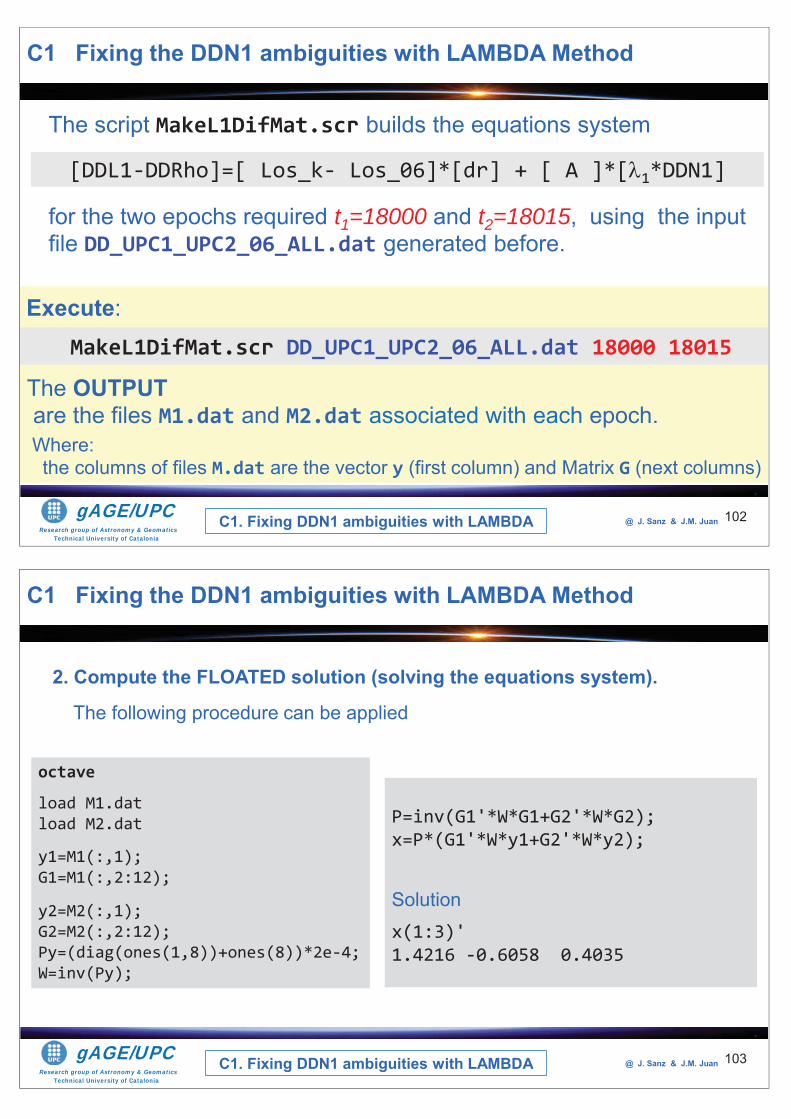
Research group of Astronomy & GeomaticsTechnical University of Catalonia
gAGE/UPC @ J. Sanz & J.M. Juan 102
The script MakeL1DifMat.scr builds the equations system
The OUTPUTare the files M1.dat and M2.dat associated with each epoch.
for the two epochs required t1=18000 and t2=18015, using the input file DD_UPC1_UPC2_06_ALL.dat generated before.
[DDL1-DDRho]=[ Los_k- Los_06]*[dr] + [ A ]*[ 1*DDN1]
MakeL1DifMat.scr DD_UPC1_UPC2_06_ALL.dat 18000 18015
Execute:
Where: the columns of files M.dat are the vector y (first column) and Matrix G (next columns)
C1 Fixing the DDN1 ambiguities with LAMBDA Method
C1. Fixing DDN1 ambiguities with LAMBDA
Research group of Astronomy & GeomaticsTechnical University of Catalonia
gAGE/UPC @ J. Sanz & J.M. Juan 103
2. Compute the FLOATED solution (solving the equations system).
The following procedure can be applied
octave
load M1.datload M2.dat
y1=M1(:,1);G1=M1(:,2:12);
y2=M2(:,1);G2=M2(:,2:12);Py=(diag(ones(1,8))+ones(8))*2e-4;W=inv(Py);
P=inv(G1'*W*G1+G2'*W*G2);x=P*(G1'*W*y1+G2'*W*y2);
Solutionx(1:3)'1.4216 -0.6058 0.4035
C1 Fixing the DDN1 ambiguities with LAMBDA Method
C1. Fixing DDN1 ambiguities with LAMBDA
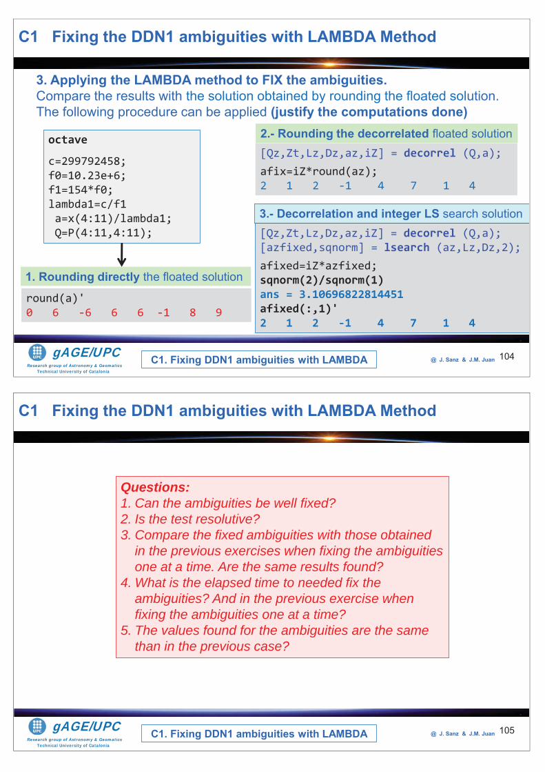
Research group of Astronomy & GeomaticsTechnical University of Catalonia
gAGE/UPC @ J. Sanz & J.M. Juan 104
3. Applying the LAMBDA method to FIX the ambiguities. Compare the results with the solution obtained by rounding the floated solution. The following procedure can be applied (justify the computations done)
octave
c=299792458;f0=10.23e+6;f1=154*f0;lambda1=c/f1a=x(4:11)/lambda1;Q=P(4:11,4:11); [Qz,Zt,Lz,Dz,az,iZ] = decorrel (Q,a);
[azfixed,sqnorm] = lsearch (az,Lz,Dz,2);afixed=iZ*azfixed;sqnorm(2)/sqnorm(1)ans = 3.10696822814451afixed(:,1)'2 1 2 -1 4 7 1 4
round(a)'0 6 -6 6 6 -1 8 9
1. Rounding directly the floated solution
3.- Decorrelation and integer LS search solution
[Qz,Zt,Lz,Dz,az,iZ] = decorrel (Q,a);afix=iZ*round(az);2 1 2 -1 4 7 1 4
2.- Rounding the decorrelated floated solution
C1 Fixing the DDN1 ambiguities with LAMBDA Method
C1. Fixing DDN1 ambiguities with LAMBDA
Research group of Astronomy & GeomaticsTechnical University of Catalonia
gAGE/UPC @ J. Sanz & J.M. Juan 105
Questions: 1. Can the ambiguities be well fixed?2. Is the test resolutive?3. Compare the fixed ambiguities with those obtained
in the previous exercises when fixing the ambiguities one at a time. Are the same results found?
4. What is the elapsed time to needed fix the ambiguities? And in the previous exercise when fixing the ambiguities one at a time?
5. The values found for the ambiguities are the same than in the previous case?
C1 Fixing the DDN1 ambiguities with LAMBDA Method
C1. Fixing DDN1 ambiguities with LAMBDA
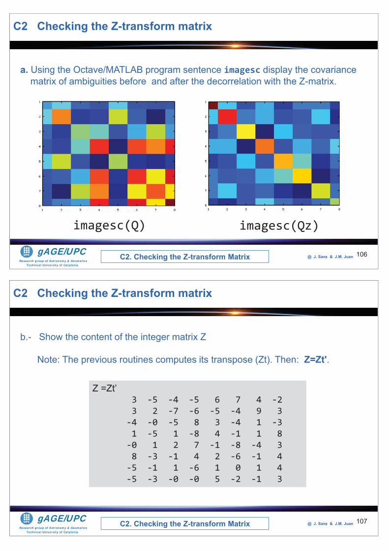
Research group of Astronomy & GeomaticsTechnical University of Catalonia
gAGE/UPC @ J. Sanz & J.M. Juan 106
C2 Checking the Z-transform matrix
C2. Checking the Z-transform Matrix
a. Using the Octave/MATLAB program sentence imagesc display the covariance matrix of ambiguities before and after the decorrelation with the Z-matrix.
imagesc(Q) imagesc(Qz)
Research group of Astronomy & GeomaticsTechnical University of Catalonia
gAGE/UPC @ J. Sanz & J.M. Juan 107
C2 Checking the Z-transform matrix
C2. Checking the Z-transform Matrix
b.- Show the content of the integer matrix Z
Note: The previous routines computes its transpose (Zt). Then: Z=Zt'.
Z =Zt’3 -5 -4 -5 6 7 4 -23 2 -7 -6 -5 -4 9 3
-4 -0 -5 8 3 -4 1 -31 -5 1 -8 4 -1 1 8
-0 1 2 7 -1 -8 -4 38 -3 -1 4 2 -6 -1 4
-5 -1 1 -6 1 0 1 4-5 -3 -0 -0 5 -2 -1 3
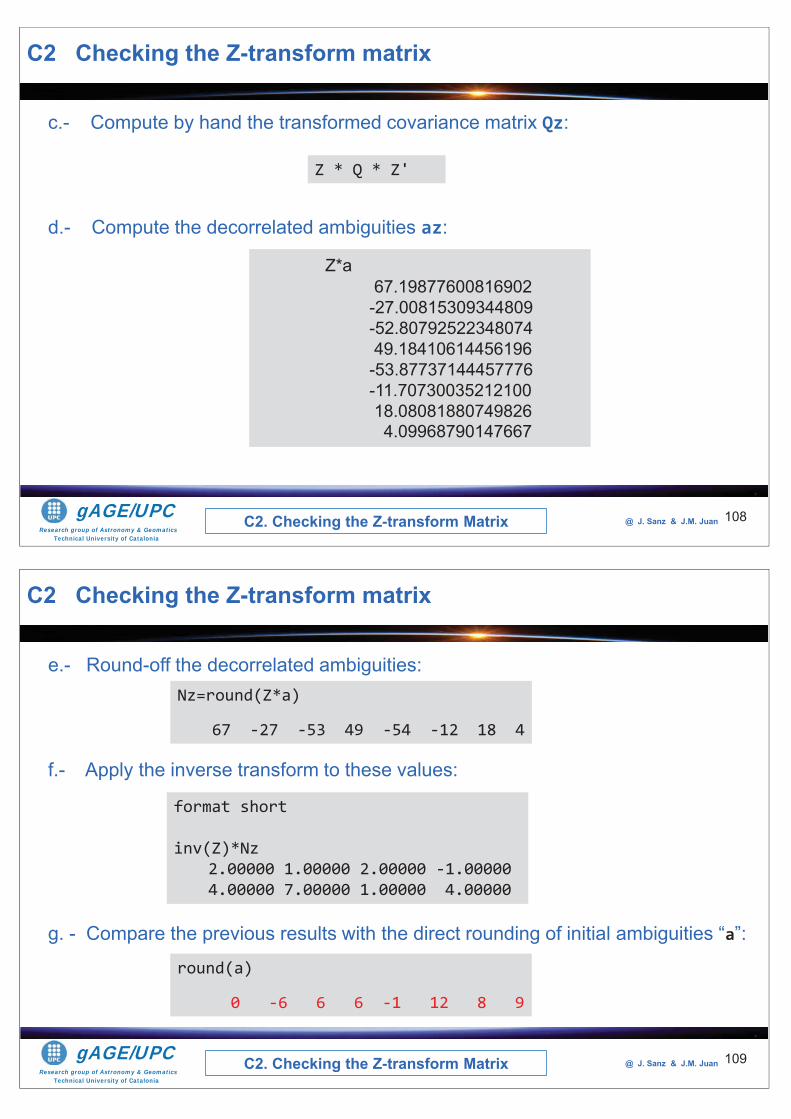
Research group of Astronomy & GeomaticsTechnical University of Catalonia
gAGE/UPC @ J. Sanz & J.M. Juan 108
C2 Checking the Z-transform matrix
C2. Checking the Z-transform Matrix
c.- Compute by hand the transformed covariance matrix Qz:
d.- Compute the decorrelated ambiguities az:
Z * Q * Z'
Z*a67.19877600816902
-27.00815309344809-52.8079252234807449.18410614456196
-53.87737144457776-11.7073003521210018.080818807498264.09968790147667
Research group of Astronomy & GeomaticsTechnical University of Catalonia
gAGE/UPC @ J. Sanz & J.M. Juan 109
C2 Checking the Z-transform matrix
C2. Checking the Z-transform Matrix
e.- Round-off the decorrelated ambiguities:
f.- Apply the inverse transform to these values:
g. - Compare the previous results with the direct rounding of initial ambiguities “a”:
Nz=round(Z*a)
67 -27 -53 49 -54 -12 18 4
format short
inv(Z)*Nz2.00000 1.00000 2.00000 -1.00000 4.00000 7.00000 1.00000 4.00000
round(a)
0 -6 6 6 -1 12 8 9
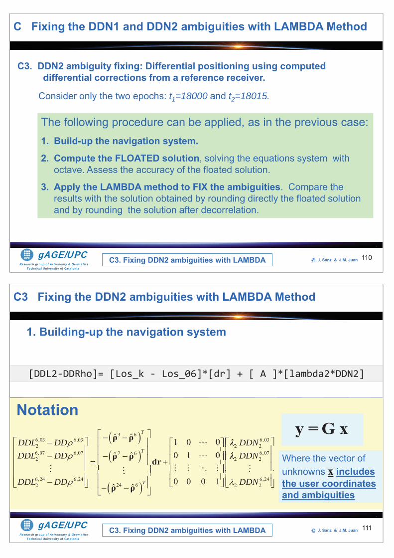
Research group of Astronomy & GeomaticsTechnical University of Catalonia
gAGE/UPC @ J. Sanz & J.M. Juan 110
C3. DDN2 ambiguity fixing: Differential positioning using computed differential corrections from a reference receiver.
Consider only the two epochs: t1=18000 and t2=18015.
The following procedure can be applied, as in the previous case:1. Build-up the navigation system.
2. Compute the FLOATED solution, solving the equations system with octave. Assess the accuracy of the floated solution.
3. Apply the LAMBDA method to FIX the ambiguities. Compare the results with the solution obtained by rounding directly the floated solution and by rounding the solution after decorrelation.
C3. Fixing DDN2 ambiguities with LAMBDA
C Fixing the DDN1 and DDN2 ambiguities with LAMBDA Method
Research group of Astronomy & GeomaticsTechnical University of Catalonia
gAGE/UPC @ J. Sanz & J.M. Juan
1. Building-up the navigation system
111
[DDL2-DDRho]= [Los_k - Los_06]*[dr] + [ A ]*[lambda2*DDN2]
3 66,03 6,03 6,032 2 26,07 6,07 6,077 62 2 2
6,24 6,24 6,2424 62 2 2
ˆ ˆ 1 0 00 1 0ˆ ˆ
0 0 0 1ˆ ˆ
T
T
T
DDL DD DDNDDL DD DDN
DDL DD DDN
ρ ρ
ρ ρ dr
ρ ρ
2220 222
22220
Notation
Where the vector of unknowns x includes the user coordinates and ambiguities
y =G x
C3 Fixing the DDN2 ambiguities with LAMBDA Method
C3. Fixing DDN2 ambiguities with LAMBDA
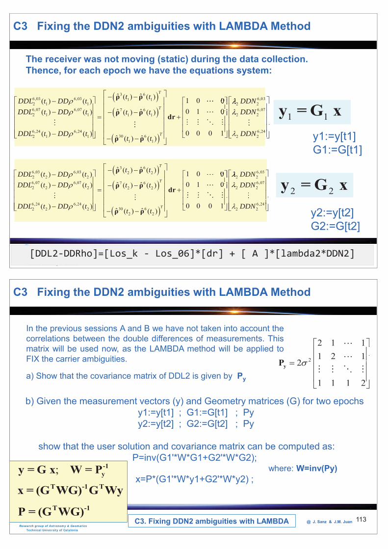
Research group of Astronomy & GeomaticsTechnical University of Catalonia
gAGE/UPC @ J. Sanz & J.M. Juan 112[DDL2-DDRho]=[Los_k - Los_06]*[dr] + [ A ]*[lambda2*DDN2]
3 66,03 6,03 6,031 12 1 1 2 26,07 6,07 7 62 1 1 21 1
6,24 6,2430 62 1 1
1 1
ˆ ˆ( ) ( ) 1 0 0( ) ( )0 1 0ˆ ˆ( ) ( ) ( ) ( )
0 0 0 1( ) ( ) ˆ ˆ( ) ( )
T
T
T
t tDDL t DD t DDNDDL t DD t t t
DDL t DD tt t
ρ ρ
ρ ρ dr
ρ ρ
22220
2220000 6,072
6,242 2
DDN
DDN
3 66,03 6,03 6,032 22 2 2 2 26,07 6,07 7 62 2 2 22 2
6,24 6,2430 62 2 2
2 2
ˆ ˆ( ) ( ) 1 0 0( ) ( )0 1 0ˆ ˆ( ) ( ) ( ) ( )
0 0 0 1( ) ( ) ˆ ˆ( ) ( )
T
T
T
t tDDL t DD t DDNDDL t DD t t t
DDL t DD tt t
ρ ρ
ρ ρ dr
ρ ρ
22220
2220000 6,072
6,242 2
DDN
DDN
1 1y =G xy1:=y[t1] G1:=G[t1]
2 2y = G xy2:=y[t2] G2:=G[t2]
The receiver was not moving (static) during the data collection. Thence, for each epoch we have the equations system:
C3 Fixing the DDN2 ambiguities with LAMBDA Method
Research group of Astronomy & GeomaticsTechnical University of Catalonia
gAGE/UPC @ J. Sanz & J.M. Juan 113
In the previous sessions A and B we have not taken into account thecorrelations between the double differences of measurements. Thismatrix will be used now, as the LAMBDA method will be applied toFIX the carrier ambiguities.
a) Show that the covariance matrix of DDL2 is given by Py
2
2 1 11 2 1
2
1 1 1 2
1111
yP
b) Given the measurement vectors (y) and Geometry matrices (G) for two epochsy1:=y[t1] ; G1:=G[t1] ; Pyy2:=y[t2] ; G2:=G[t2] ; Py
show that the user solution and covariance matrix can be computed as:P=inv(G1'*W*G1+G2'*W*G2);
where: W=inv(Py)x=P*(G1'*W*y1+G2'*W*y2) ;
; -1yy = G x W = P
T -1 Tx = (G WG) G WyT -1P = (G WG)
C3 Fixing the DDN2 ambiguities with LAMBDA Method
C3. Fixing DDN2 ambiguities with LAMBDA
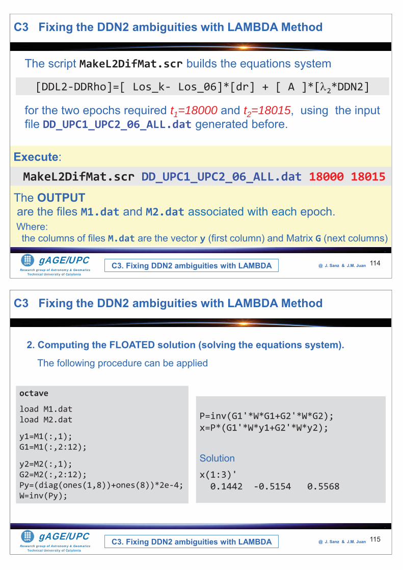
Research group of Astronomy & GeomaticsTechnical University of Catalonia
gAGE/UPC @ J. Sanz & J.M. Juan 114
The script MakeL2DifMat.scr builds the equations system
The OUTPUTare the files M1.dat and M2.dat associated with each epoch.
for the two epochs required t1=18000 and t2=18015, using the input file DD_UPC1_UPC2_06_ALL.dat generated before.
[DDL2-DDRho]=[ Los_k- Los_06]*[dr] + [ A ]*[ 2*DDN2]
MakeL2DifMat.scr DD_UPC1_UPC2_06_ALL.dat 18000 18015Execute:
Where: the columns of files M.dat are the vector y (first column) and Matrix G (next columns)
C3 Fixing the DDN2 ambiguities with LAMBDA Method
C3. Fixing DDN2 ambiguities with LAMBDA
Research group of Astronomy & GeomaticsTechnical University of Catalonia
gAGE/UPC @ J. Sanz & J.M. Juan 115
2. Computing the FLOATED solution (solving the equations system).
The following procedure can be applied
octave
load M1.datload M2.dat
y1=M1(:,1);G1=M1(:,2:12);
y2=M2(:,1);G2=M2(:,2:12);Py=(diag(ones(1,8))+ones(8))*2e-4;W=inv(Py);
P=inv(G1'*W*G1+G2'*W*G2);x=P*(G1'*W*y1+G2'*W*y2);
Solutionx(1:3)'
0.1442 -0.5154 0.5568
C3 Fixing the DDN2 ambiguities with LAMBDA Method
C3. Fixing DDN2 ambiguities with LAMBDA
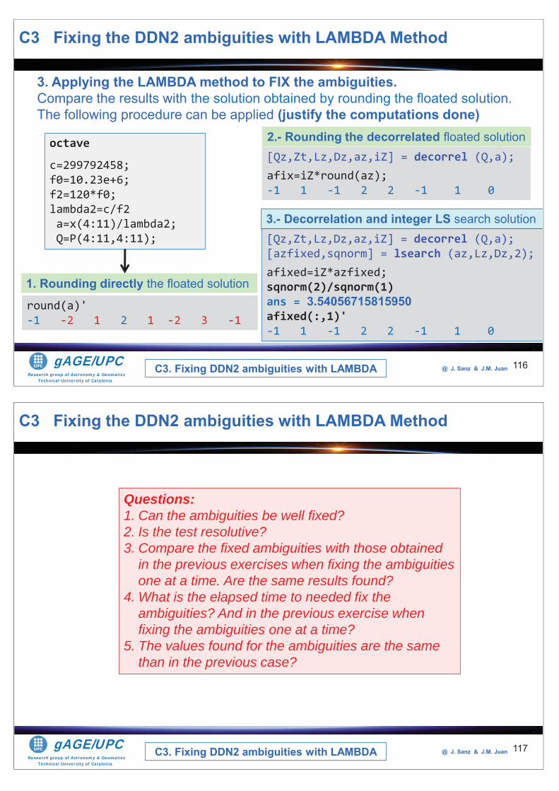
Research group of Astronomy & GeomaticsTechnical University of Catalonia
gAGE/UPC @ J. Sanz & J.M. Juan 116
3. Applying the LAMBDA method to FIX the ambiguities. Compare the results with the solution obtained by rounding the floated solution. The following procedure can be applied (justify the computations done)
octave
c=299792458;f0=10.23e+6;f2=120*f0;lambda2=c/f2a=x(4:11)/lambda2;Q=P(4:11,4:11); [Qz,Zt,Lz,Dz,az,iZ] = decorrel (Q,a);
[azfixed,sqnorm] = lsearch (az,Lz,Dz,2);afixed=iZ*azfixed;sqnorm(2)/sqnorm(1)ans = 3.54056715815950afixed(:,1)'-1 1 -1 2 2 -1 1 0
round(a)'-1 -2 1 2 1 -2 3 -1
1. Rounding directly the floated solution
3.- Decorrelation and integer LS search solution
[Qz,Zt,Lz,Dz,az,iZ] = decorrel (Q,a);afix=iZ*round(az);-1 1 -1 2 2 -1 1 0
2.- Rounding the decorrelated floated solution
C3 Fixing the DDN2 ambiguities with LAMBDA Method
C3. Fixing DDN2 ambiguities with LAMBDA
Research group of Astronomy & GeomaticsTechnical University of Catalonia
gAGE/UPC @ J. Sanz & J.M. Juan 117
Questions: 1. Can the ambiguities be well fixed?2. Is the test resolutive?3. Compare the fixed ambiguities with those obtained
in the previous exercises when fixing the ambiguities one at a time. Are the same results found?
4. What is the elapsed time to needed fix the ambiguities? And in the previous exercise when fixing the ambiguities one at a time?
5. The values found for the ambiguities are the same than in the previous case?
C3 Fixing the DDN2 ambiguities with LAMBDA Method
C3. Fixing DDN2 ambiguities with LAMBDA
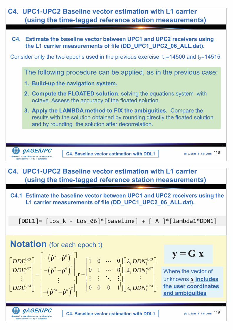
Research group of Astronomy & GeomaticsTechnical University of Catalonia
gAGE/UPC @ J. Sanz & J.M. Juan 118
C4. Estimate the baseline vector between UPC1 and UPC2 receivers using the L1 carrier measurements of file (DD_UPC1_UPC2_06_ALL.dat).
Consider only the two epochs used in the previous exercise: t1=14500 and t2=14515
C4. Baseline vector estimation with DDL1
C4. UPC1-UPC2 Baseline vector estimation with L1 carrier(using the time-tagged reference station measurements)
The following procedure can be applied, as in the previous case:1. Build-up the navigation system.
2. Compute the FLOATED solution, solving the equations system with octave. Assess the accuracy of the floated solution.
3. Apply the LAMBDA method to FIX the ambiguities. Compare the results with the solution obtained by rounding directly the floated solution and by rounding the solution after decorrelation.
Research group of Astronomy & GeomaticsTechnical University of Catalonia
gAGE/UPC @ J. Sanz & J.M. Juan
C4.1 Estimate the baseline vector between UPC1 and UPC2 receivers using the L1 carrier measurements of file (DD_UPC1_UPC2_06_ALL.dat).
119
[DDL1]= [Los_k - Los_06]*[baseline] + [ A ]*[lambda1*DDN1]
3 66,03 6,031 1 16,07 6,077 61 1 1
6,24 6,2424 61 1 1
ˆ ˆ 1 0 00 1 0ˆ ˆ
0 0 0 1ˆ ˆ
T
T
T
DDL DDNDDL DDN
DDL DDN
ρ ρ
ρ ρ r
ρ ρ
1110 111
11110
Notation (for each epoch t)
Where the vector of unknowns x includes the user coordinates and ambiguities
y =G x
C4. Baseline vector estimation with DDL1
C4. UPC1-UPC2 Baseline vector estimation with L1 carrier(using the time-tagged reference station measurements)

Research group of Astronomy & GeomaticsTechnical University of Catalonia
gAGE/UPC @ J. Sanz & J.M. Juan 120[DDL1]=[Los_k - Los_06]*[baseline] + [ A ]*[lambda1*DDN1]
3 66,03 6,031 11 1 1 16,07 6,077 61 1 1 11 1
6,24 6,2424 61 1 1 1
1 1
ˆ ˆ( ) ( ) 1 0 0( )0 1 0ˆ ˆ( ) ( ) ( )
0 0 0 1( ) ˆ ˆ( ) ( )
T
T
T
t tDDL t DDNDDL t DDNt t
DDL t DDNt t
ρ ρ
ρ ρ r
ρ ρ
1110 111
11110
3 66,03 6,032 21 2 1 16,07 6,077 61 2 1 12 2
6,24 6,2424 61 2 1 1
2 2
ˆ ˆ( ) ( ) 1 0 0( )0 1 0ˆ ˆ( ) ( ) ( )
0 0 0 1( ) ˆ ˆ( ) ( )
T
T
T
t tDDL t DDNDDL t DDNt t
DDL t DDNt t
ρ ρ
ρ ρ r
ρ ρ
1110 111
11110
1 1y =G xy1:=y[t1] G1:=G[t1]
2 2y = G xy2:=y[t2] G2:=G[t2]
The receiver was not moving (static) during the data collection. Therefore, for each epoch we have the equations system:
C4. UPC1-UPC2 Baseline vector estimation with L1 carrier(using the time-tagged reference station measurements)
Research group of Astronomy & GeomaticsTechnical University of Catalonia
gAGE/UPC @ J. Sanz & J.M. JuanC4. Baseline vector estimation with DDL1 121
In the previous sessions A and B we have not taken into account thecorrelations between the double differences of measurements. Thismatrix will be used now, as the LAMBDA method will be applied toFIX the carrier ambiguities.
a) Show that the covariance matrix of DDL1 is given by Py
2
2 1 11 2 1
2
1 1 1 2
1111
yP
b) Given the measurement vectors (y) and Geometry matrices (G) for two epochsy1:=y[t1] ; G1:=G[t1] ; Pyy2:=y[t2] ; G2:=G[t2] ; Py
show that the user solution and covariance matrix can be computed as:P=inv(G1'*W*G1+G2'*W*G2);
where: W=inv(Py)x=P*(G1'*W*y1+G2'*W*y2) ;
; -1yy = G x W = P
T -1 Tx = (G WG) G WyT -1P = (G WG)
C4. UPC1-UPC2 Baseline vector estimation with L1 carrier(using the time-tagged reference station measurements)
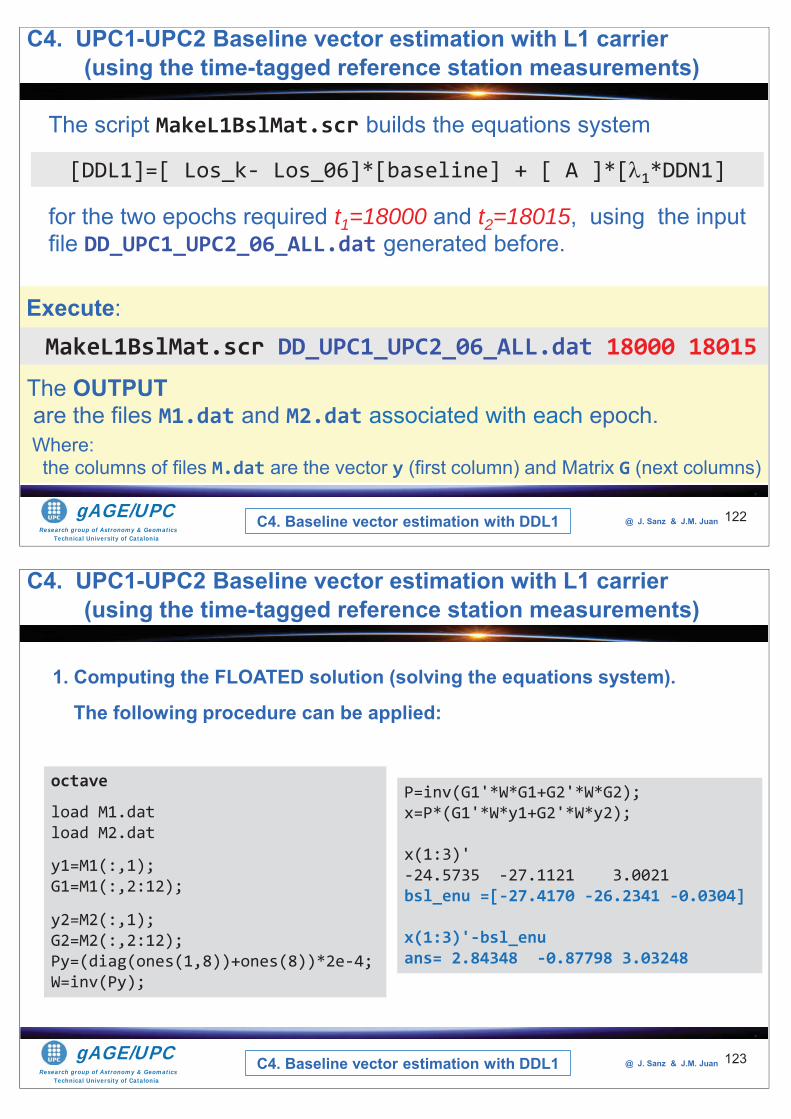
Research group of Astronomy & GeomaticsTechnical University of Catalonia
gAGE/UPC @ J. Sanz & J.M. Juan 122
The script MakeL1BslMat.scr builds the equations system
The OUTPUTare the files M1.dat and M2.dat associated with each epoch.
for the two epochs required t1=18000 and t2=18015, using the input file DD_UPC1_UPC2_06_ALL.dat generated before.
[DDL1]=[ Los_k- Los_06]*[baseline] + [ A ]*[ 1*DDN1]
MakeL1BslMat.scr DD_UPC1_UPC2_06_ALL.dat 18000 18015Execute:
Where: the columns of files M.dat are the vector y (first column) and Matrix G (next columns)
C4. Baseline vector estimation with DDL1
C4. UPC1-UPC2 Baseline vector estimation with L1 carrier(using the time-tagged reference station measurements)
Research group of Astronomy & GeomaticsTechnical University of Catalonia
gAGE/UPC @ J. Sanz & J.M. Juan 123
1. Computing the FLOATED solution (solving the equations system).
The following procedure can be applied:
octave
load M1.datload M2.dat
y1=M1(:,1);G1=M1(:,2:12);
y2=M2(:,1);G2=M2(:,2:12);Py=(diag(ones(1,8))+ones(8))*2e-4;W=inv(Py);
P=inv(G1'*W*G1+G2'*W*G2);x=P*(G1'*W*y1+G2'*W*y2);
x(1:3)'-24.5735 -27.1121 3.0021bsl_enu =[-27.4170 -26.2341 -0.0304]
x(1:3)'-bsl_enuans= 2.84348 -0.87798 3.03248
C4. UPC1-UPC2 Baseline vector estimation with L1 carrier(using the time-tagged reference station measurements)
C4. Baseline vector estimation with DDL1
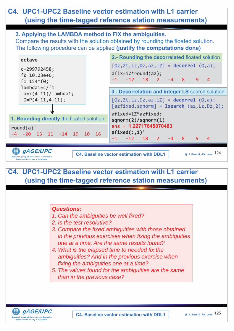
Research group of Astronomy & GeomaticsTechnical University of Catalonia
gAGE/UPC @ J. Sanz & J.M. Juan 124
3. Applying the LAMBDA method to FIX the ambiguities. Compare the results with the solution obtained by rounding the floated solution. The following procedure can be applied (justify the computations done)
octave
c=299792458;f0=10.23e+6;f1=154*f0;lambda1=c/f1a=x(4:11)/lambda1;Q=P(4:11,4:11); [Qz,Zt,Lz,Dz,az,iZ] = decorrel (Q,a);
[azfixed,sqnorm] = lsearch (az,Lz,Dz,2);afixed=iZ*azfixed;sqnorm(2)/sqnorm(1)ans = 1.22717645070483afixed(:,1)'-1 -12 18 2 -4 8 9 4
round(a)'-4 -20 13 11 -14 19 10 16
1. Rounding directly the floated solution
3.- Decorrelation and integer LS search solution
[Qz,Zt,Lz,Dz,az,iZ] = decorrel (Q,a);afix=iZ*round(az);-1 -12 18 2 -4 8 9 4
2.- Rounding the decorrelated floated solution
C4. UPC1-UPC2 Baseline vector estimation with L1 carrier(using the time-tagged reference station measurements)
C4. Baseline vector estimation with DDL1
Research group of Astronomy & GeomaticsTechnical University of Catalonia
gAGE/UPC @ J. Sanz & J.M. Juan 125
Questions: 1. Can the ambiguities be well fixed?2. Is the test resolutive?3. Compare the fixed ambiguities with those obtained
in the previous exercises when fixing the ambiguities one at a time. Are the same results found?
4. What is the elapsed time to needed fix the ambiguities? And in the previous exercise when fixing the ambiguities one at a time?
5. The values found for the ambiguities are the same than in the previous case?
C4. UPC1-UPC2 Baseline vector estimation with L1 carrier(using the time-tagged reference station measurements)
C4. Baseline vector estimation with DDL1
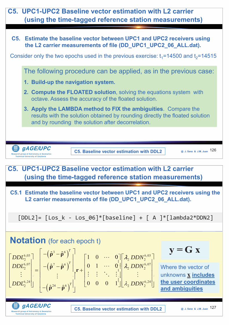
Research group of Astronomy & GeomaticsTechnical University of Catalonia
gAGE/UPC @ J. Sanz & J.M. Juan 126
C5. Estimate the baseline vector between UPC1 and UPC2 receivers using the L2 carrier measurements of file (DD_UPC1_UPC2_06_ALL.dat).
Consider only the two epochs used in the previous exercise: t1=14500 and t2=14515
C5. UPC1-UPC2 Baseline vector estimation with L2 carrier(using the time-tagged reference station measurements)
The following procedure can be applied, as in the previous case:1. Build-up the navigation system.
2. Compute the FLOATED solution, solving the equations system with octave. Assess the accuracy of the floated solution.
3. Apply the LAMBDA method to FIX the ambiguities. Compare the results with the solution obtained by rounding directly the floated solution and by rounding the solution after decorrelation.
C5. Baseline vector estimation with DDL2
Research group of Astronomy & GeomaticsTechnical University of Catalonia
gAGE/UPC @ J. Sanz & J.M. Juan
C5.1 Estimate the baseline vector between UPC1 and UPC2 receivers using the L2 carrier measurements of file (DD_UPC1_UPC2_06_ALL.dat).
127
[DDL2]= [Los_k - Los_06]*[baseline] + [ A ]*[lambda2*DDN2]
3 66,03 6,032 2 26,07 6,077 62 2 2
6,24 6,2424 62 2 2
ˆ ˆ 1 0 00 1 0ˆ ˆ
0 0 0 1ˆ ˆ
T
T
T
DDL DDNDDL DDN
DDL DDN
ρ ρ
ρ ρ r
ρ ρ
2220 222
22220
Notation (for each epoch t)
Where the vector of unknowns x includes the user coordinates and ambiguities
y =G x
C5. UPC1-UPC2 Baseline vector estimation with L2 carrier(using the time-tagged reference station measurements)
C5. Baseline vector estimation with DDL2
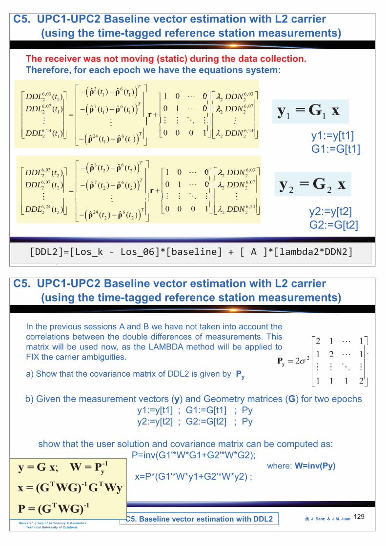
Research group of Astronomy & GeomaticsTechnical University of Catalonia
gAGE/UPC @ J. Sanz & J.M. Juan 128[DDL2]=[Los_k - Los_06]*[baseline] + [ A ]*[lambda2*DDN2]
3 66,03 6,031 12 1 2 26,07 6,077 62 1 2 21 1
6,24 6,2424 62 1 2 2
1 1
ˆ ˆ( ) ( ) 1 0 0( )0 1 0ˆ ˆ( ) ( ) ( )
0 0 0 1( ) ˆ ˆ( ) ( )
T
T
T
t tDDL t DDNDDL t DDNt t
DDL t DDNt t
ρ ρ
ρ ρ r
ρ ρ
2220 222
22220
3 66,03 6,032 22 2 2 26,07 6,077 62 2 2 22 2
6,24 6,2424 62 2 2 2
2 2
ˆ ˆ( ) ( ) 1 0 0( )0 1 0ˆ ˆ( ) ( ) ( )
0 0 0 1( ) ˆ ˆ( ) ( )
T
T
T
t tDDL t DDNDDL t DDNt t
DDL t DDNt t
ρ ρ
ρ ρ r
ρ ρ
2220 222
22220
1 1y =G xy1:=y[t1] G1:=G[t1]
2 2y = G xy2:=y[t2] G2:=G[t2]
The receiver was not moving (static) during the data collection. Therefore, for each epoch we have the equations system:
C5. UPC1-UPC2 Baseline vector estimation with L2 carrier(using the time-tagged reference station measurements)
Research group of Astronomy & GeomaticsTechnical University of Catalonia
gAGE/UPC @ J. Sanz & J.M. JuanC5. Baseline vector estimation with DDL2 129
In the previous sessions A and B we have not taken into account thecorrelations between the double differences of measurements. Thismatrix will be used now, as the LAMBDA method will be applied toFIX the carrier ambiguities.
a) Show that the covariance matrix of DDL2 is given by Py
2
2 1 11 2 1
2
1 1 1 2
1111
yP
b) Given the measurement vectors (y) and Geometry matrices (G) for two epochsy1:=y[t1] ; G1:=G[t1] ; Pyy2:=y[t2] ; G2:=G[t2] ; Py
show that the user solution and covariance matrix can be computed as:P=inv(G1'*W*G1+G2'*W*G2);
where: W=inv(Py)x=P*(G1'*W*y1+G2'*W*y2) ;
; -1yy = G x W = P
T -1 Tx = (G WG) G WyT -1P = (G WG)
C5. UPC1-UPC2 Baseline vector estimation with L2 carrier(using the time-tagged reference station measurements)
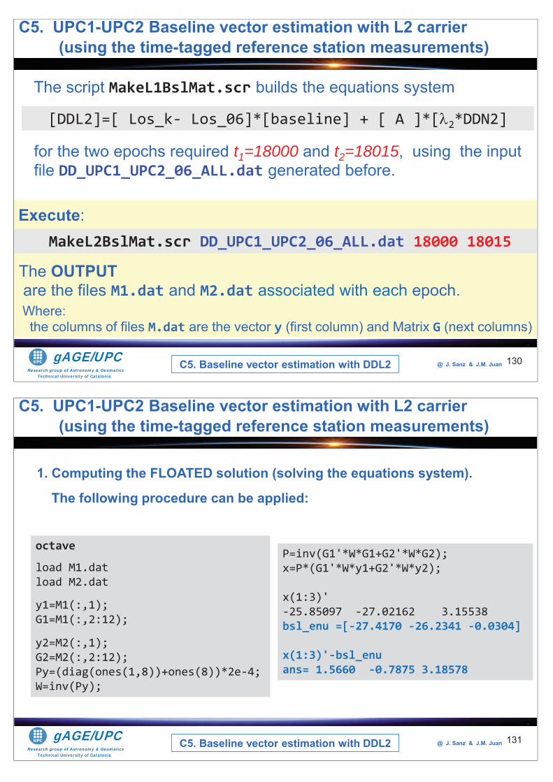
Research group of Astronomy & GeomaticsTechnical University of Catalonia
gAGE/UPC @ J. Sanz & J.M. Juan 130
The script MakeL1BslMat.scr builds the equations system
The OUTPUTare the files M1.dat and M2.dat associated with each epoch.
for the two epochs required t1=18000 and t2=18015, using the input file DD_UPC1_UPC2_06_ALL.dat generated before.
[DDL2]=[ Los_k- Los_06]*[baseline] + [ A ]*[ 2*DDN2]
MakeL2BslMat.scr DD_UPC1_UPC2_06_ALL.dat 18000 18015
Execute:
Where: the columns of files M.dat are the vector y (first column) and Matrix G (next columns)
C5. UPC1-UPC2 Baseline vector estimation with L2 carrier(using the time-tagged reference station measurements)
C5. Baseline vector estimation with DDL2
Research group of Astronomy & GeomaticsTechnical University of Catalonia
gAGE/UPC @ J. Sanz & J.M. Juan 131
1. Computing the FLOATED solution (solving the equations system).
The following procedure can be applied:
octave
load M1.datload M2.dat
y1=M1(:,1);G1=M1(:,2:12);
y2=M2(:,1);G2=M2(:,2:12);Py=(diag(ones(1,8))+ones(8))*2e-4;W=inv(Py);
P=inv(G1'*W*G1+G2'*W*G2);x=P*(G1'*W*y1+G2'*W*y2);
x(1:3)'-25.85097 -27.02162 3.15538 bsl_enu =[-27.4170 -26.2341 -0.0304]
x(1:3)'-bsl_enuans= 1.5660 -0.7875 3.18578
C5. UPC1-UPC2 Baseline vector estimation with L2 carrier(using the time-tagged reference station measurements)
C5. Baseline vector estimation with DDL2
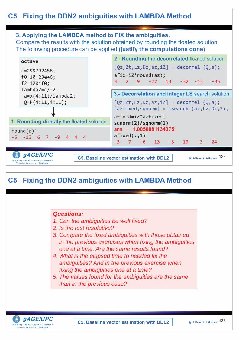
Research group of Astronomy & GeomaticsTechnical University of Catalonia
gAGE/UPC @ J. Sanz & J.M. Juan 132
3. Applying the LAMBDA method to FIX the ambiguities. Compare the results with the solution obtained by rounding the floated solution. The following procedure can be applied (justify the computations done)
octave
c=299792458;f0=10.23e+6;f2=120*f0;lambda2=c/f2a=x(4:11)/lambda2;Q=P(4:11,4:11); [Qz,Zt,Lz,Dz,az,iZ] = decorrel (Q,a);
[azfixed,sqnorm] = lsearch (az,Lz,Dz,2);afixed=iZ*azfixed;sqnorm(2)/sqnorm(1)ans = 1.00508811343751afixed(:,1)'-3 7 -6 13 -3 19 -3 24
round(a)'-5 -13 6 7 -9 4 4 4
1. Rounding directly the floated solution
3.- Decorrelation and integer LS search solution
[Qz,Zt,Lz,Dz,az,iZ] = decorrel (Q,a);afix=iZ*round(az);3 2 9 -27 13 -32 -13 -35
2.- Rounding the decorrelated floated solution
C5 Fixing the DDN2 ambiguities with LAMBDA Method
C5. Baseline vector estimation with DDL2
Research group of Astronomy & GeomaticsTechnical University of Catalonia
gAGE/UPC @ J. Sanz & J.M. Juan 133
Questions: 1. Can the ambiguities be well fixed?2. Is the test resolutive?3. Compare the fixed ambiguities with those obtained
in the previous exercises when fixing the ambiguities one at a time. Are the same results found?
4. What is the elapsed time to needed fix the ambiguities? And in the previous exercise when fixing the ambiguities one at a time?
5. The values found for the ambiguities are the same than in the previous case?
C5 Fixing the DDN2 ambiguities with LAMBDA Method
C5. Baseline vector estimation with DDL2
Research group of Astronomy & GeomaticsTechnical University of Catalonia
gAGE/UPC @ J. Sanz & J.M. Juan 134
Thanks for yourattention
Research group of Astronomy & GeomaticsTechnical University of Catalonia
gAGE/UPC @ J. Sanz & J.M. Juan
• To the University of Delft for the MATLAB files of LAMBDA method.• To Adrià Rovira-Garcia for his contribution to the editing of this material
and gLAB updating and integrating this learning material into the GLUE.
The ESA/UPC GNSS-Lab Tool suite (gLAB) has been developed under theESA Education Office contract N. P1081434.
Acknowledgements

Research group of Astronomy & GeomaticsTechnical University of Catalonia
gAGE/UPC @ J. Sanz & J.M. Juan 1
Tutorial 5Analysis of propagation effects from
GNSS observables based on laboratory exercises
Contact: [email protected] site: http://www.gage.upc.edu
Slides associated to gLAB version 2.0.0
Research group of Astronomy & GeomaticsTechnical University of Catalonia
gAGE/UPC @ J. Sanz & J.M. Juan
Authorship statement
The authorship of this material and the Intellectual Property Rights are owned by J. Sanz Subirana and J.M. Juan Zornoza.
These slides can be obtained either from the server http://www.gage.upc.edu,or [email protected]. Any partial reproduction should be previously authorized by the authors, clearly referring to the slides used.
This authorship statement must be kept intact and unchanged at all times.
2
Research group of Astronomy & GeomaticsTechnical University of Catalonia
gAGE/UPC @ J. Sanz & J.M. Juan
IntroductionThe gLAB tool suiteExamples of GNSS Data Processing using gLABLaboratory session organization
LABORATORY SessionStarting up your laptopBasic: Introductory lab exercises: Iono & Posit, SF, storm,TIDs
Medium: Laboratory Work Projects: LWP1 to LWP4Advanced: Homework
OVERVIEW
3
Research group of Astronomy & GeomaticsTechnical University of Catalonia
gAGE/UPC @ J. Sanz & J.M. Juan 4
This tutorial is devoted to analysing and assessing different issues associated with GNSS signal propagation effects in the atmosphere. The laboratory exercises will be developed with actual GPS measurements, and processed with the ESA/UPC GNSS-Lab Tool suite (gLAB), which is an interactive software package for GNSS data processing and analysis. All software tools (including gLAB) and associated files for the laboratory session are included in the USB stick delivered to those who attend the lecture.The laboratory session will consist of a set of exercises organized in three different levels of difficulty (Basic, Medium and Advanced). A set of introductory examples range from a first glance assessment of the ionosphere effects on single frequency positioning, and Zenith Tropospheric Delays estimate to showing different perturbation effects in the ionosphere (Solar Flair, Halloween storm, TIDs). Electron density profiles (Ne) retrieval, bending effects analysis (phase excess rate depicture), as well as in-depth analysis of the code-carrier ionosphere divergence on single-frequency smoothed codes and the second order ionospheric effects are analysed in detail in four Laboratory Work Projects. Other topics are given as homework.The target is to provide the participants with a wide range of selected exercises to choose from, according their interests and their level of knowledge of these topics.
Introduction

Research group of Astronomy & GeomaticsTechnical University of Catalonia
gAGE/UPC @ J. Sanz & J.M. Juan
IntroductionThe gLAB tool suiteExamples of GNSS Data Processing using gLABLaboratory session organization
LABORATORY SessionStarting up your laptopBasic: Introductory lab exercises: Iono & Posit, SF, storm,TIDs
Medium: Laboratory Work Projects: LWP1 to LWP4Advanced: Homework
OVERVIEW
5
Research group of Astronomy & GeomaticsTechnical University of Catalonia
gAGE/UPC @ J. Sanz & J.M. Juan 6
gLAB has been developed under the ESA Education Office contract N. P1081434.
The gLAB Tool suite
Main features:• High Accuracy Positioning
capability.• Fully configurable.• Easy to use.• Access to internal computations.
The GNSS-Lab Tool suite (gLAB) is an interactive multipurpose educational and professional package for GNSS Data Processing and Analysis.

Research group of Astronomy & GeomaticsTechnical University of Catalonia
gAGE/UPC @ J. Sanz & J.M. Juan 7
Students/Newcomers:• Easy to use: Intuitive GUI.• Explanations: Tooltips over the different GUI options.• Guidelines: Several error and warning messages.
Templates for pre-configured processing.
Professionals/Experts:• Powerful tool with High Accuracy Positioning capability.• Fast to configure and use: Templates and carefully chosen defaults.• Can be executed in command-line and included in batch processing.
The gLAB Tool suite
Research group of Astronomy & GeomaticsTechnical University of Catalonia
gAGE/UPC @ J. Sanz & J.M. Juan 8
In order to widen the tool availability, gLAB Software has been designed to work in both Windows and Linux environments.
The package contains:• Windows binaries (with an installable file).• Linux .tgz file.• Source code (to compile it in both Linux and Windows OS)
under an Apache 2.0 license.• Example data files.• Software User Manual.• HTML files describing the standard formats.
hh group o
gA
The gLAB Tool suite
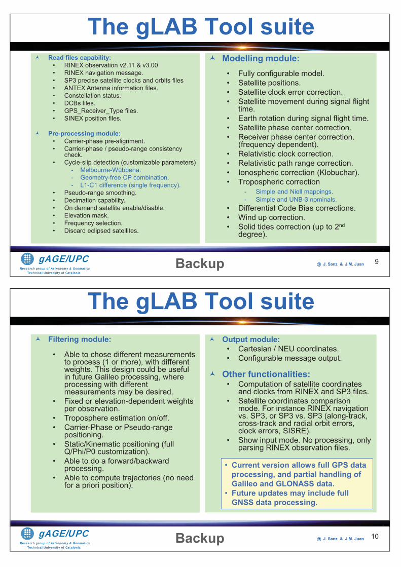
Research group of Astronomy & GeomaticsTechnical University of Catalonia
gAGE/UPC @ J. Sanz & J.M. Juan
Modelling module:• Fully configurable model.• Satellite positions.• Satellite clock error correction.• Satellite movement during signal flight
time.• Earth rotation during signal flight time.• Satellite phase center correction.• Receiver phase center correction.
(frequency dependent).• Relativistic clock correction.• Relativistic path range correction.• Ionospheric correction (Klobuchar).• Tropospheric correction
- Simple and Niell mappings.- Simple and UNB-3 nominals.
• Differential Code Bias corrections.• Wind up correction.• Solid tides correction (up to 2nd
degree).
9
Read files capability:• RINEX observation v2.11 & v3.00• RINEX navigation message.• SP3 precise satellite clocks and orbits files• ANTEX Antenna information files.• Constellation status.• DCBs files.• GPS_Receiver_Type files.• SINEX position files.
Pre-processing module:• Carrier-phase pre-alignment.• Carrier-phase / pseudo-range consistency
check.• Cycle-slip detection (customizable parameters)
- Melbourne-Wübbena.- Geometry-free CP combination.- L1-C1 difference (single frequency).
• Pseudo-range smoothing.• Decimation capability.• On demand satellite enable/disable.• Elevation mask.• Frequency selection.• Discard eclipsed satellites.
The gLAB Tool suite
Backup
Research group of Astronomy & GeomaticsTechnical University of Catalonia
gAGE/UPC @ J. Sanz & J.M. Juan 10
Filtering module:
• Able to chose different measurements to process (1 or more), with different weights. This design could be useful in future Galileo processing, where processing with different measurements may be desired.
• Fixed or elevation-dependent weights per observation.
• Troposphere estimation on/off.• Carrier-Phase or Pseudo-range
positioning.• Static/Kinematic positioning (full
Q/Phi/P0 customization).• Able to do a forward/backward
processing.• Able to compute trajectories (no need
for a priori position).
Output module:• Cartesian / NEU coordinates.• Configurable message output.
Other functionalities:• Computation of satellite coordinates
and clocks from RINEX and SP3 files.• Satellite coordinates comparison
mode. For instance RINEX navigation vs. SP3, or SP3 vs. SP3 (along-track, cross-track and radial orbit errors, clock errors, SISRE).
• Show input mode. No processing, only parsing RINEX observation files.
• Current version allows full GPS data processing, and partial handling of Galileo and GLONASS data.
• Future updates may include full GNSS data processing.
The gLAB Tool suite
Backup

Research group of Astronomy & GeomaticsTechnical University of Catalonia
gAGE/UPC @ J. Sanz & J.M. Juan
GNSS learning material package
• GNSS Book: Complete book with theory, practical examples, and with a Laboratory course on GNSS Data Processing & Analysis [R-1].
• gLAB tool suite: Source code and binary software files, plus configuration files, allowing processing GNSS data from standard formats. The options are fully configurable through a GUI.
• gAGE-GLUE: Bootable USB stick with a full environment ready to use; based on LINUX (Ubuntu) OS.
Image courtesy of USAF Research Laboratory
GPS Data Processing: Code and PhaseAlgorithms, Techniques and Recipes
Research group of Astronomy & GeomaticsSatellite Navigation, LLC
http://www.gage.es
gAGE-NAV Manuel Hernández PajaresJosé Miguel Juan Zornoza
Jaume Sanz Subirana
11
Includes three different parts, allowing participants to follow either a guided or a self-learning GNSS course:
Research group of Astronomy & GeomaticsTechnical University of Catalonia
gAGE/UPC @ J. Sanz & J.M. Juan
IntroductionThe gLAB tool suiteExamples of GNSS processing using gLABLaboratory session organization
LABORATORY SessionStarting up your laptopBasic: Introductory lab exercises: Iono & Posit, SF, storm,TIDs
Medium: Laboratory Work Projects: LWP1 to LWP4Advanced: Homework
OVERVIEW
12
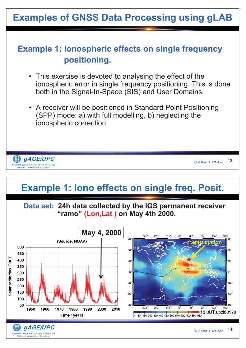
Research group of Astronomy & GeomaticsTechnical University of Catalonia
gAGE/UPC @ J. Sanz & J.M. Juan
Example 1: Ionospheric effects on single frequency positioning.
• This exercise is devoted to analysing the effect of the ionospheric error in single frequency positioning. This is done both in the Signal-In-Space (SIS) and User Domains.
• A receiver will be positioned in Standard Point Positioning (SPP) mode: a) with full modelling, b) neglecting the ionospheric correction.
13
Examples of GNSS Data Processing using gLAB
Research group of Astronomy & GeomaticsTechnical University of Catalonia
gAGE/UPC @ J. Sanz & J.M. Juan
May 4, 2000
Data set: 24h data collected by the IGS permanent receiver “ramo” (Lon,Lat ) on May 4th 2000.
Example 1: Iono effects on single freq. Posit.
14
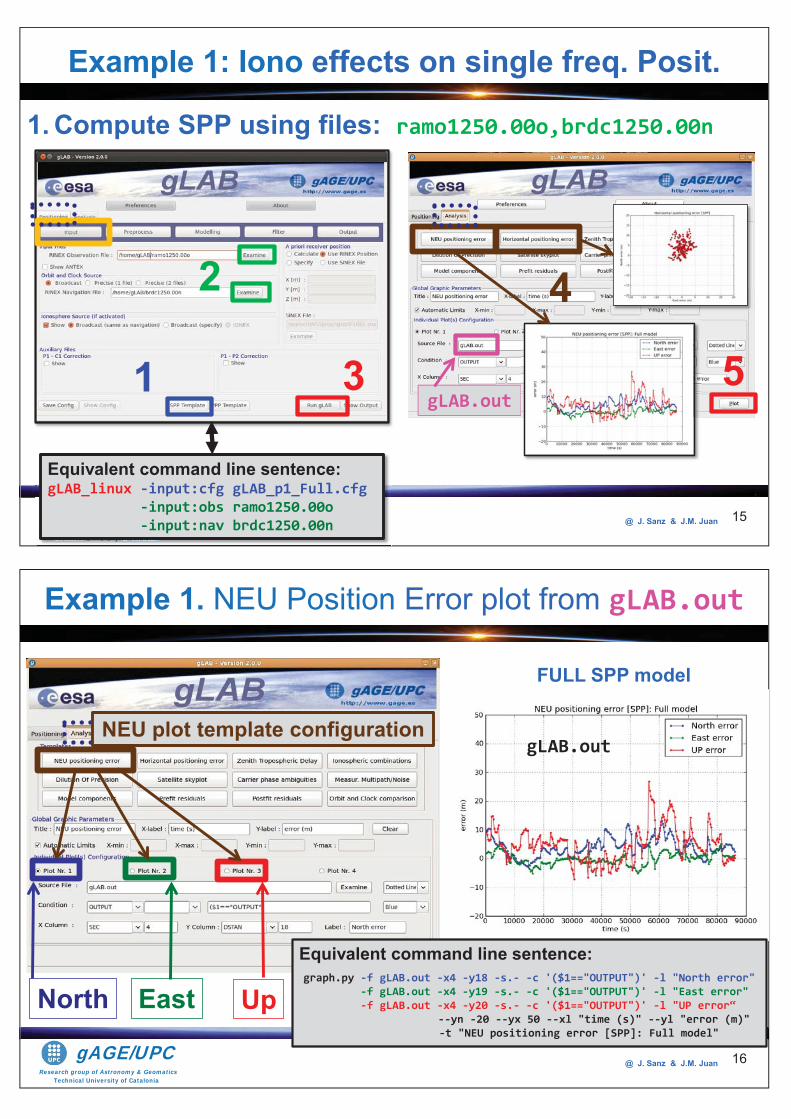
Research group of Astronomy & GeomaticsTechnical University of Catalonia
gAGE/UPC @ J. Sanz & J.M. Juan
1. Compute SPP using files: ramo1250.00o,brdc1250.00n
15
1
2
3
4
5gLAB.out
ecTechn caical U eUnive yyys yrsity oof Ca aCatalo aoniaRR
TechnTechnicalicalTechnTechnicalical UniveUniversityrsityUniveUniversityrsity ofofofof CatalCataloniaoniaCatalCataloniaonia
Equivalent command line sentence:gLAB_linux -input:cfg gLAB_p1_Full.cfg -input:obs ramo1250.00o -input:nav brdc1250.00n
Example 1: Iono effects on single freq. Posit.
Research group of Astronomy & GeomaticsTechnical University of Catalonia
gAGE/UPC @ J. Sanz & J.M. Juan 16
Example 1. NEU Position Error plot from gLAB.out
North East Up
FULL SPP model
NEU plot template configuration
Equivalent command line sentence:
graph.py -f gLAB.out -x4 -y18 -s.- -c '($1=="OUTPUT")' -l "North error" -f gLAB.out -x4 -y19 -s.- -c '($1=="OUTPUT")' -l "East error"
-f gLAB.out -x4 -y20 -s.- -c '($1=="OUTPUT")' -l "UP error“ --yn -20 --yx 50 --xl "time (s)" --yl "error (m)" -t "NEU positioning error [SPP]: Full model"
gLAB.out
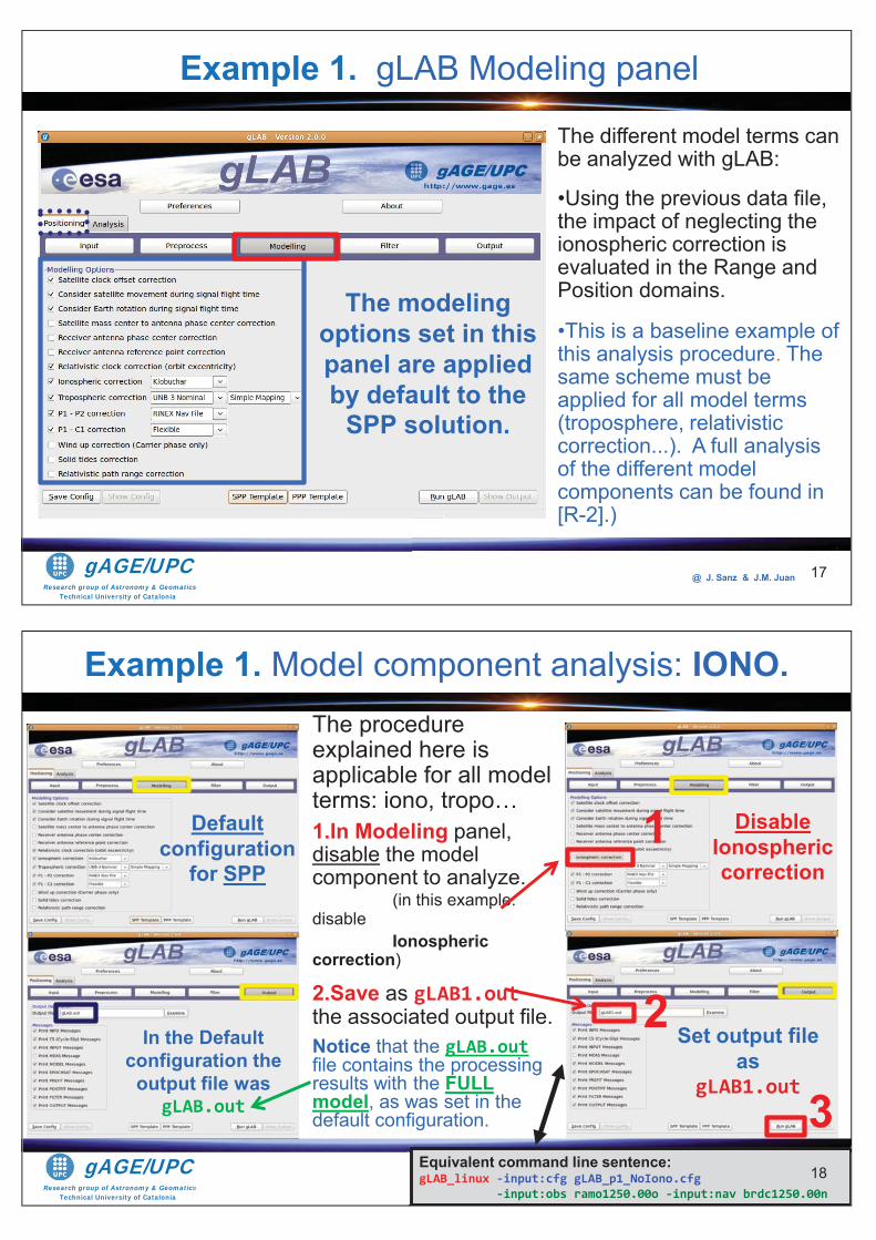
Research group of Astronomy & GeomaticsTechnical University of Catalonia
gAGE/UPC @ J. Sanz & J.M. Juan
The different model terms can be analyzed with gLAB:
•Using the previous data file, the impact of neglecting the ionospheric correction is evaluated in the Range and Position domains.
•This is a baseline example of this analysis procedure. The same scheme must be applied for all model terms (troposphere, relativistic correction...). A full analysis of the different model components can be found in [R-2].)
The modeling options set in this panel are applied by default to the
SPP solution.
17
Example 1. gLAB Modeling panel
Research group of Astronomy & GeomaticsTechnical University of Catalonia
gAGE/UPC @ J. Sanz & J.M. Juan 18
Example 1. Model component analysis: IONO.
Default configuration
for SPP
In the Default configuration the
output file was gLAB.out
icsics
C
Set output file as
gLAB1.out
z &
Disable Ionosphericcorrection
The procedure explained here is applicable for all model terms: iono, tropo…1.In Modeling panel, disable the model component to analyze.
(in this example: disable
Ionospheric correction)
2.Save as gLAB1.out the associated output file.Notice that the gLAB.outfile contains the processing results with the FULLmodel, as was set in the default configuration.
1
2
3Equivalent command line sentence:gLAB_linux -input:cfg gLAB_p1_NoIono.cfg -input:obs ramo1250.00o -input:nav brdc1250.00n
18
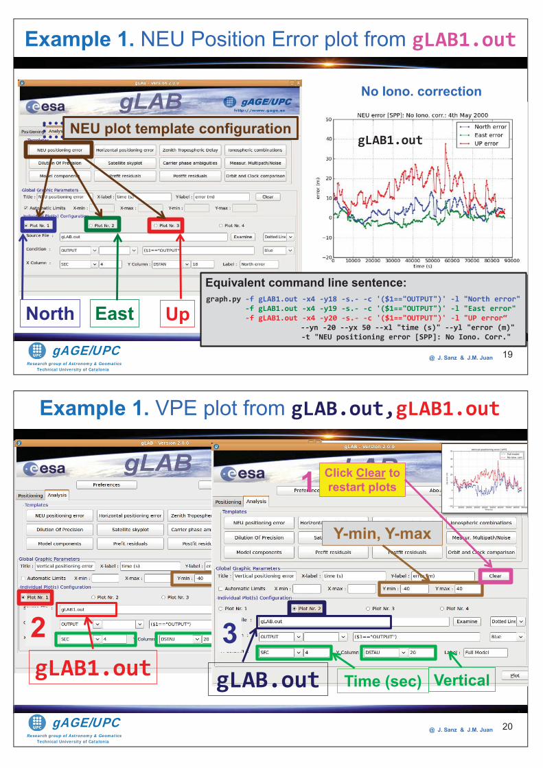
Research group of Astronomy & GeomaticsTechnical University of Catalonia
gAGE/UPC @ J. Sanz & J.M. Juan 19
Example 1. NEU Position Error plot from gLAB1.out
North East Up
No Iono. correction
NEU plot template configuration
Equivalent command line sentence:
graph.py -f gLAB1.out -x4 -y18 -s.- -c '($1=="OUTPUT")' -l "North error" -f gLAB1.out -x4 -y19 -s.- -c '($1=="OUTPUT")' -l "East error"
-f gLAB1.out -x4 -y20 -s.- -c '($1=="OUTPUT")' -l "UP error“ --yn -20 --yx 50 --xl "time (s)" --yl "error (m)" -t "NEU positioning error [SPP]: No Iono. Corr."
gLAB1.out
Research group of Astronomy & GeomaticsTechnical University of Catalonia
gAGE/UPC @ J. Sanz & J.M. Juan 20
gLAB1.out gLAB.out Time (sec) Vertical
Y-min, Y-max
Example 1. VPE plot from gLAB.out,gLAB1.out
Click Clear to restart plots1
2 3
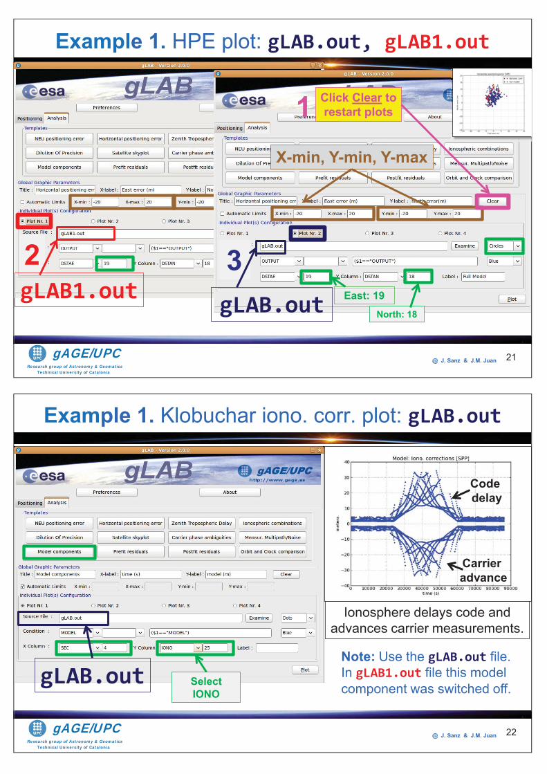
Research group of Astronomy & GeomaticsTechnical University of Catalonia
gAGE/UPC @ J. Sanz & J.M. Juan 21
Example 1. HPE plot: gLAB.out, gLAB1.out
gLAB.out East: 19North: 18
X-min, Y-min, Y-max
Click Clear to restart plots1
2 3gLAB1.out
Research group of Astronomy & GeomaticsTechnical University of Catalonia
gAGE/UPC @ J. Sanz & J.M. Juan 22
Example 1. Klobuchar iono. corr. plot: gLAB.out
gLAB.out SelectIONO
Note: Use the gLAB.out file.In gLAB1.out file this model component was switched off.
Code delay
Ionosphere delays code and advances carrier measurements.
Carrier advance
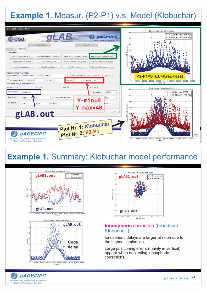
Research group of Astronomy & GeomaticsTechnical University of Catalonia
gAGE/UPC @ J. Sanz & J.M. Juan@@@@@@@@@@@@@@@@ JJJ... SanSannSannnnnnnzzz &&&&&&&&&&&&&&&& JJJJJJJJJJJJJJJJJJJJJJJJJJ...MMMMMMMMMMMMMMMM... JuaJuaaJuaaaaaaaaJJJJJJ nnn 23
Example 1. Measur. (P2-P1) v.s. Model (Klobuchar)
gLAB.out
Y-min=0 Y-max=40
P2-P1=STEC+Krec+Ksat
Research group of Astronomy & GeomaticsTechnical University of Catalonia
gAGE/UPC @ J. Sanz & J.M. Juan 24
Example 1. Summary: Klobuchar model performance
gLAB.out
gLAB1.out
gLAB.out
Code delay
gLAB.out
gLAB1.out
Ionospheric correction (broadcast Klobuchar )Ionospheric delays are larger at noon due to the higher illumination. Large positioning errors (mainly in vertical) appear when neglecting ionosphericcorrections.
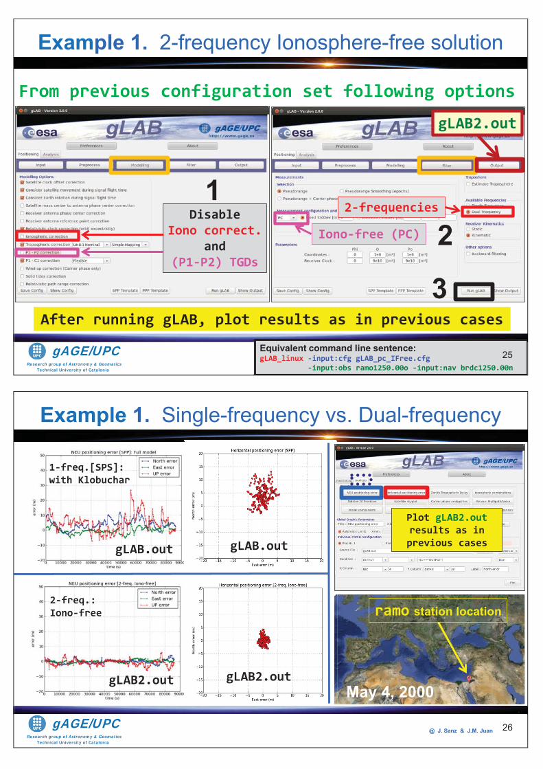
Research group of Astronomy & GeomaticsTechnical University of Catalonia
gAGE/UPC @ J. Sanz & J.M. Juan
From previous configuration set following options
25
Disable Iono correct.
and (P1-P2) TGDs
1Iono-free (PC)
2-frequencies
2
3After running gLAB, plot results as in previous cases
Equivalent command line sentence:gLAB_linux -input:cfg gLAB_pc_IFree.cfg -input:obs ramo1250.00o -input:nav brdc1250.00n
gLAB2.out
Example 1. 2-frequency Ionosphere-free solution
25
Research group of Astronomy & GeomaticsTechnical University of Catalonia
gAGE/UPC @ J. Sanz & J.M. Juan 26
2-freq.: Iono-free
1-freq.[SPS]: with Klobuchar
ramo station location
Plot gLAB2.out results as in previous cases
May 4, 2000
gLAB.out gLAB.out
gLAB2.out gLAB2.out
Example 1. Single-frequency vs. Dual-frequency
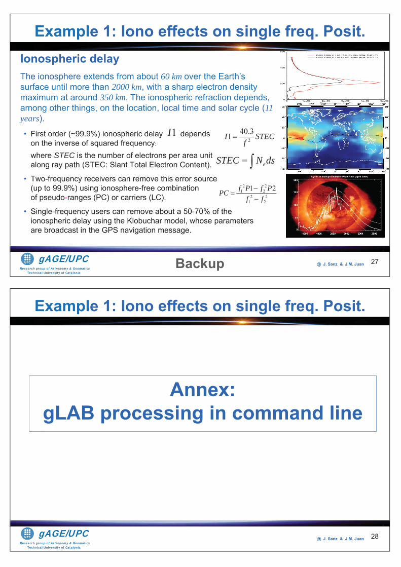
Research group of Astronomy & GeomaticsTechnical University of Catalonia
gAGE/UPC @ J. Sanz & J.M. Juan
• First order (~99.9%) ionospheric delay depends on the inverse of squared frequency:
where STEC is the number of electrons per area unit along ray path (STEC: Slant Total Electron Content).
• Two-frequency receivers can remove this error source (up to 99.9%) using ionosphere-free combination of pseudo-ranges (PC) or carriers (LC).
• Single-frequency users can remove about a 50-70% of the ionospheric delay using the Klobuchar model, whose parameters are broadcast in the GPS navigation message.
27
eSTEC N ds
2 21 2
2 21 2
1 2f P f PPCf f
1I
Ionospheric delayThe ionosphere extends from about 60 km over the Earth’s surface until more than 2000 km, with a sharp electron density maximum at around 350 km. The ionospheric refraction depends, among other things, on the location, local time and solar cycle (11 years).
Backup
240.31I STECf
Example 1: Iono effects on single freq. Posit.
Research group of Astronomy & GeomaticsTechnical University of Catalonia
gAGE/UPC @ J. Sanz & J.M. Juan 28
Annex: gLAB processing in command line
Example 1: Iono effects on single freq. Posit.
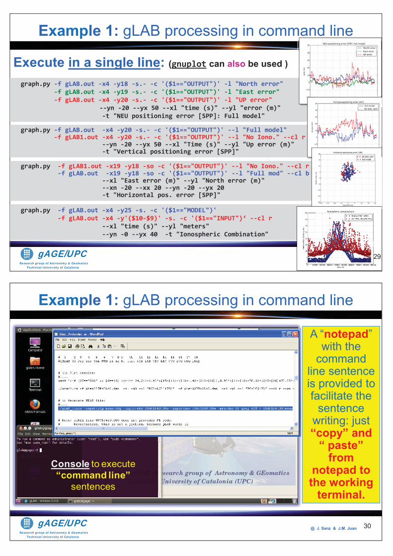
Research group of Astronomy & GeomaticsTechnical University of Catalonia
gAGE/UPC @ J. Sanz & J.M. Juan 29
Execute in a single line: (gnuplot can also be used )
graph.py -f gLAB.out -x4 -y20 -s.- -c '($1=="OUTPUT")' --l "Full model" -f gLAB1.out -x4 -y20 -s.- -c '($1=="OUTPUT")' --l "No Iono." --cl r --yn -20 --yx 50 --xl "Time (s)" --yl "Up error (m)" -t "Vertical positioning error [SPP]"
graph.py -f gLAB1.out -x19 -y18 -so -c '($1=="OUTPUT")' --l "No Iono." --cl r -f gLAB.out -x19 -y18 -so -c '($1=="OUTPUT")' --l "Full mod" --cl b --xl "East error (m)" --yl "North error (m)" --xn -20 --xx 20 --yn -20 --yx 20 -t "Horizontal pos. error [SPP]"
graph.py -f gLAB.out -x4 -y25 -s. -c '($1=="MODEL")' -f gLAB.out -x4 -y'($10-$9)' -s. -c '($1=="INPUT")‘ --cl r --xl "time (s)" --yl "meters" --yn -0 --yx 40 -t "Ionospheric Combination"
graph.py -f gLAB.out -x4 -y18 -s.- -c '($1=="OUTPUT")' -l "North error" -f gLAB.out -x4 -y19 -s.- -c '($1=="OUTPUT")' -l "East error" -f gLAB.out -x4 -y20 -s.- -c '($1=="OUTPUT")' -l "UP error" --yn -20 --yx 50 --xl "time (s)" --yl "error (m)" -t "NEU positioning error [SPP]: Full model"
Example 1: gLAB processing in command line
@@@@@@@@@@@@@@@@@@@@@@@@@@@@@@@@@@@@@@@@@@@@@@@@@@@@@@@@@@@@@@@@@@@@@@@@@@@@@@@@@@@@@@@@@@@@@@@@@@@@@@@@@@@@@@@@@@@@@@@@@@@@@@@@@@@@@ JJJJJJJJJJJJJJJJJJJJJJJJJJJJJJJJJJJJJJJJJJJJJJJJJJJJJJJJJJJJJJJJJJJJJJJJJJJ........... SanSannSanSanSanSanSaSanaSanSanaaaaSanSanSanSanSanSananSannnSanaSanaanaaaaaSanSanSSSSSanSanSanSannaaaaSaSSSSSannSanaaSaaSSSSSanSanSanSannaanaaSSSSaSSSSSSannnaaanSSSSSanSSaSSSSSSaSannanSSSSSannSanaannaSaSannanannaSSSSSSS naSSSSaSaS nnaaSSSaSanaaSSaaSaSSSSSSS zzzzz &&& JJJ.MMM. uaJuaJuaJuaJuauaaaJuaJuauauauuuauJuauuJuuaJuaaJuaaaJuauuuJuauauauJuuJuauaauuJuuuauaaaaaJuauuuauauuJuuaaauaaaaauauauuJuuuuuuaauaaaaaaJuauuuuuaaauaauuuuJuJuaJuaJuaJ auuJJuauauauJuaJJJuaaaauuJJJuJuaaaaauuJJJ aaJJJJJJJJJ nnnnnnnnnnnnnnnnnnnnnnnnnnnnnnnnnnnnnnnnnnnnnnnnnnnnnnnn 22929292929299292929292929999292922229999299929222999992999929222222999999292222292999999929299292999922229292922229999999299999922222222222999999292999292929222929292999299292929292929929992929292992999999929292929929292929299229999999929292992222229999999992922222229999929222222299222299922922292929299222299999922222999999292929922999992222222229222222929292922992922229229922222 29
Research group of Astronomy & GeomaticsTechnical University of Catalonia
gAGE/UPC @ J. Sanz & J.M. Juan 30
Console to execute “command line”
sentences
Example 1: gLAB processing in command line
A “notepad”with the
command line sentence is provided to facilitate the
sentence writing: just “copy” and
“ paste” from
notepad to the working
terminal.
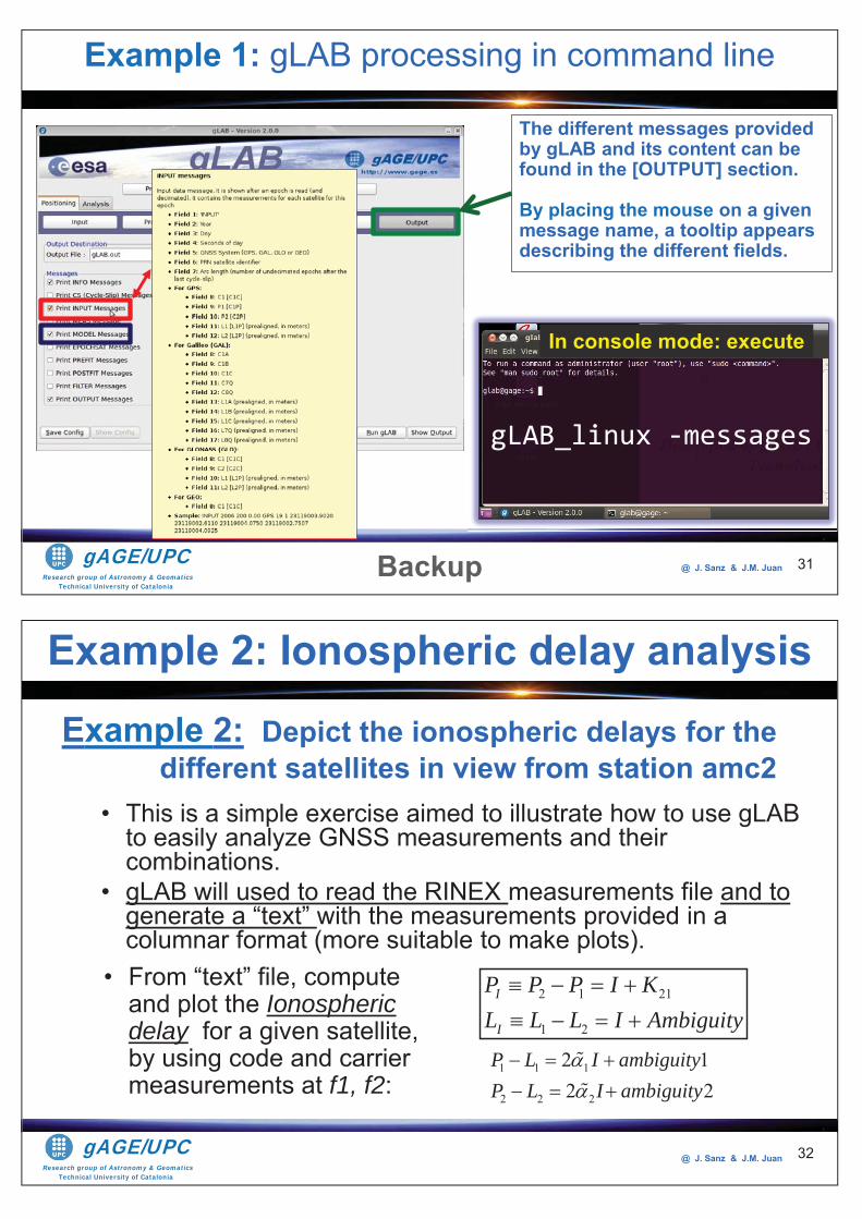
Research group of Astronomy & GeomaticsTechnical University of Catalonia
gAGE/UPC @ J. Sanz & J.M. Juan 31
The different messages provided by gLAB and its content can be found in the [OUTPUT] section.
By placing the mouse on a given message name, a tooltip appears describing the different fields.
Backup
gLAB_linux -messages
In console mode: execute
Example 1: gLAB processing in command line
Research group of Astronomy & GeomaticsTechnical University of Catalonia
gAGE/UPC @ J. Sanz & J.M. Juan
Example 2: Depict the ionospheric delays for the different satellites in view from station amc2
• This is a simple exercise aimed to illustrate how to use gLAB to easily analyze GNSS measurements and their combinations.
• gLAB will used to read the RINEX measurements file and to generate a “text” with the measurements provided in a columnar format (more suitable to make plots).
Example 2: Ionospheric delay analysis
• From “text” file, compute and plot the Ionosphericdelay for a given satellite, by using code and carrier measurements at f1, f2:
2 1 21
1 2
I
I
P P P I KL L L I Ambiguity
1 1 1
2 2 2
2 12 2
P L I ambiguityP L I ambiguity
32
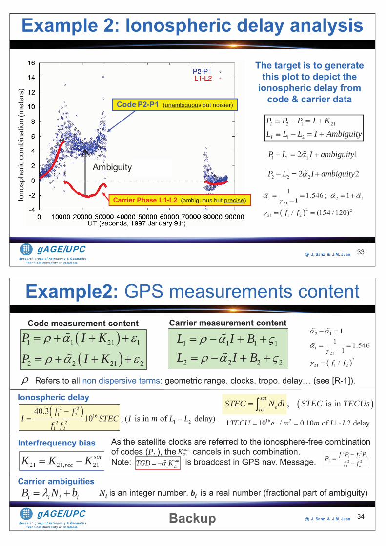
Research group of Astronomy & GeomaticsTechnical University of Catalonia
gAGE/UPC @ J. Sanz & J.M. Juan 33
Example 2: Ionospheric delay analysis
The target is to generate this plot to depict the
ionospheric delay from code & carrier data
2 1 21
1 2
I
I
P P P I KL L L I Ambiguity
1 1 12 1P L I ambiguity
1 2 121
2 221 1 2
1 1.546 ; 11
/ (154 /120)f f
2 2 22 2P L I ambiguity
Carrier Phase L1-L2 (ambiguous but precise)
Code P2-P1 (unambiguous but noisier)
Ambiguity= P L
Iono
sphe
ric c
ombi
natio
n (m
eter
s)
Research group of Astronomy & GeomaticsTechnical University of Catalonia
gAGE/UPC @ J. Sanz & J.M. Juan 34
Example2: GPS measurements content
1 1 21 1
2 2 21 2
P I K
P I K1 1 1 1
2 2 2 2
L I BL I B
, is in sat
erecSTEC N dl STEC TECUs
16 21 10 / 0.10 of 1- 2 delayTECU e m m L L
2 21 2 16
1 22 21 2
40.310 ; ( is in of delay)
f fI STEC I m L L
f f
21 21, 21sat
recK K K
As the satellite clocks are referred to the ionosphere-free combination of codes (PC), the cancels in such combination. Note: is broadcast in GPS nav. Message.1 21
satTGD K
Refers to all non dispersive terms: geometric range, clocks, tropo. delay… (see [R-1]).
Ionospheric delay
Interfrequency bias21satK 2 2
1 1 2 22 2
1 2C
f P f PPf f
i i i iB N bCarrier ambiguities
Ni is an integer number. bi is a real number (fractional part of ambiguity)
2 1
121
221 1 2
11 1.546
1
/f f
Code measurement content Carrier measurement content
Backup
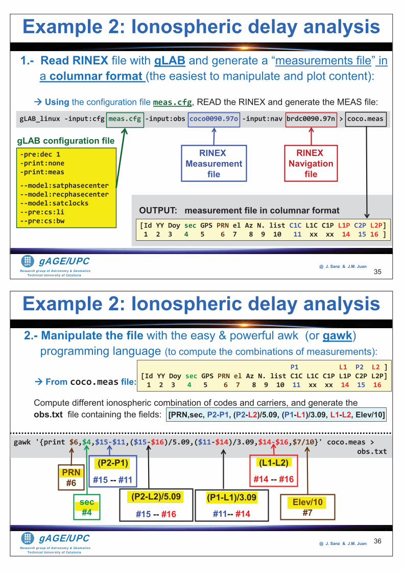
Research group of Astronomy & GeomaticsTechnical University of Catalonia
gAGE/UPC @ J. Sanz & J.M. Juan
1.- Read RINEX file with gLAB and generate a “measurements file” in a columnar format (the easiest to manipulate and plot content):
Using the configuration file meas.cfg, READ the RINEX and generate the MEAS file:
35
[Id YY Doy sec GPS PRN el Az N. list C1C L1C C1P L1P C2P L2P] 1 2 3 4 5 6 7 8 9 10 11 xx xx 14 15 16 ]
gLAB_linux -input:cfg meas.cfg -input:obs coco0090.97o -input:nav brdc0090.97n > coco.meas
Example 2: Ionospheric delay analysis
-pre:dec 1 -print:none -print:meas
--model:satphasecenter --model:recphasecenter --model:satclocks --pre:cs:li --pre:cs:bw
gLAB configuration fileRINEX
Measurementfile
RINEX Navigation
file
OUTPUT: measurement file in columnar format
Research group of Astronomy & GeomaticsTechnical University of Catalonia
gAGE/UPC @ J. Sanz & J.M. Juan
2.- Manipulate the file with the easy & powerful awk (or gawk) programming language (to compute the combinations of measurements):
From coco.meas file:
Compute different ionospheric combination of codes and carriers, and generate the obs.txt file containing the fields: [PRN,sec, P2-P1, (P2-L2)/5.09, (P1-L1)/3.09, L1-L2, Elev/10]
36
gawk '{print $6,$4,$15-$11,($15-$16)/5.09,($11-$14)/3.09,$14-$16,$7/10}' coco.meas > obs.txt
Example 2: Ionospheric delay analysis
PRN#6
sec#4
(P2-P1)
#15 -- #11
(P2-L2)/5.09
#15 -- #16
(P1-L1)/3.09
#11-- #14
(L1-L2)
#14 -- #16
Elev/10#7
P1 L1 P2 L2 ] [Id YY Doy sec GPS PRN el Az N. list C1C L1C C1P L1P C2P L2P] 1 2 3 4 5 6 7 8 9 10 11 xx xx 14 15 16
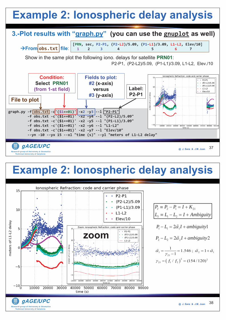
Research group of Astronomy & GeomaticsTechnical University of Catalonia
gAGE/UPC @ J. Sanz & J.M. Juan
3.-Plot results with “graph.py” (you can use the gnuplot as well)
From obs.txt file:
Show in the same plot the following iono. delays for satellite PRN01: P2-P1, (P2-L2)/5.09, (P1-L1)/3.09, L1-L2, Elev./10
37
graph.py -f obs.txt -c'($1==01)' -x2 -y3 --l "P2-P1" -f obs.txt -c'($1==01)' -x2 –y4 --l "(P2-L2)/5.09" -f obs.txt -c'($1==01)' -x2 -y5 --l "(P1-L1)/3.09" -f obs.txt -c'($1==01)' -x2 –y6 --l "L1-L2" -f obs.txt -c'($1==01)' -x2 –y7 --l "Elev/10" --yn -10 --yx 15 --xl "time (s)" --yl "meters of L1-L2 delay"
Example 2: Ionospheric delay analysis
[PRN, sec, P2-P1, (P2-L2)/5.09, (P1-L1)/3.09, L1-L2, Elev/10] 1 2 3 4 5 6 7
File to plot
Condition:Select PRN01
(from 1-st field)
Fields to plot:#2 (x-axis)
versus#3 (y-axis)
Label:P2-P1
Research group of Astronomy & GeomaticsTechnical University of Catalonia
gAGE/UPC @ J. Sanz & J.M. Juan 38
Example 2: Ionospheric delay analysis
zoom
2 1 21
1 2
I
I
P P P I KL L L I Ambiguity
1 1 12 1P L I ambiguity
1 2 121
2 221 1 2
1 1.546 ; 11
/ (154 /120)f f
2 2 22 2P L I ambiguity
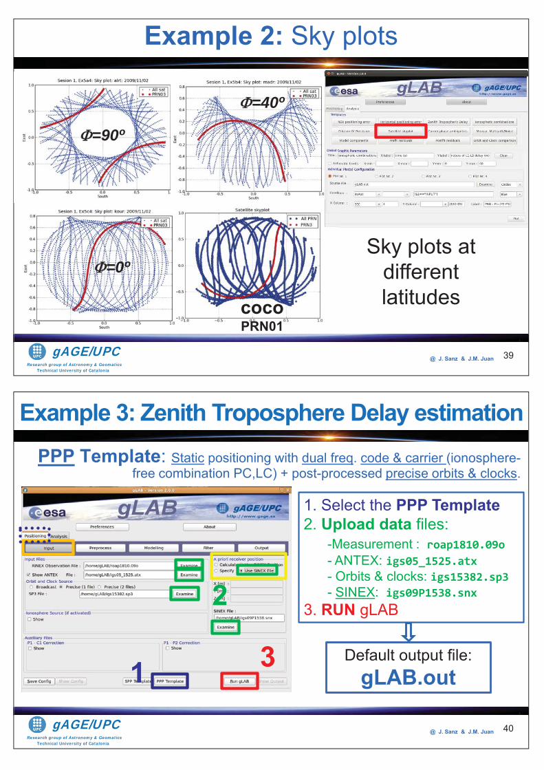
Research group of Astronomy & GeomaticsTechnical University of Catalonia
gAGE/UPC @ J. Sanz & J.M. Juan 39
cocoPRN01
Sky plots at different latitudes
Example 2: Sky plots
=90º
=40º
=0º
Research group of Astronomy & GeomaticsTechnical University of Catalonia
gAGE/UPC @ J. Sanz & J.M. Juan
PPP Template: Static positioning with dual freq. code & carrier (ionosphere-free combination PC,LC) + post-processed precise orbits & clocks.
1. Select the PPP Template 2. Upload data files:
-Measurement : roap1810.09o - ANTEX: igs05_1525.atx - Orbits & clocks: igs15382.sp3 - SINEX: igs09P1538.snx
3. RUN gLAB
Default output file:gLAB.out1
2
3
Example 3: Zenith Troposphere Delay estimation
40
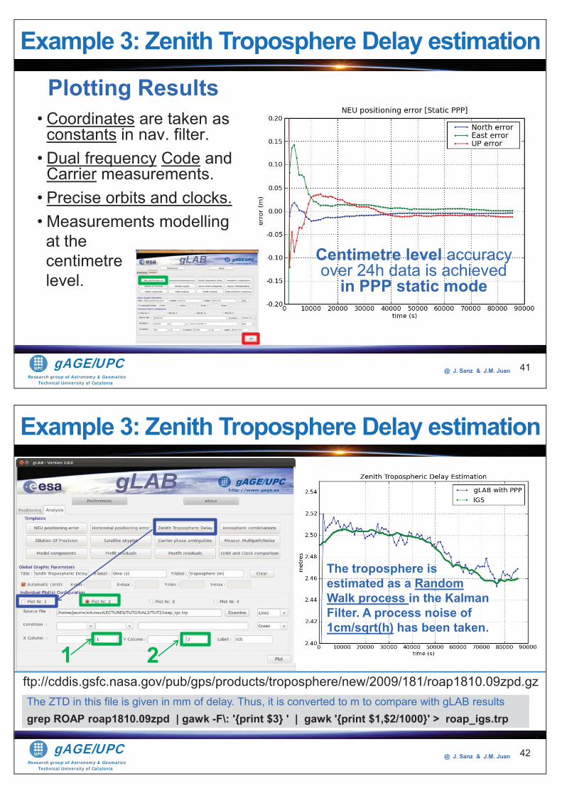
Research group of Astronomy & GeomaticsTechnical University of Catalonia
gAGE/UPC @ J. Sanz & J.M. Juan
Plotting Results• Coordinates are taken as
constants in nav. filter.• Dual frequency Code and
Carrier measurements.• Precise orbits and clocks.• Measurements modellingat the centimetrelevel.
Centimetre level accuracyover 24h data is achieved
in PPP static mode
Example 3: Zenith Troposphere Delay estimation
41
Research group of Astronomy & GeomaticsTechnical University of Catalonia
gAGE/UPC @ J. Sanz & J.M. Juan
Example 3: Zenith Troposphere Delay estimation
The ZTD in this file is given in mm of delay. Thus, it is converted to m to compare with gLAB resultsgrep ROAP roap1810.09zpd | gawk -F\: '{print $3} ' | gawk '{print $1,$2/1000}' > roap_igs.trp
ftp://cddis.gsfc.nasa.gov/pub/gps/products/troposphere/new/2009/181/roap1810.09zpd.gz
1 2
The troposphere is estimated as a Random Walk process in the Kalman Filter. A process noise of 1cm/sqrt(h) has been taken.
42
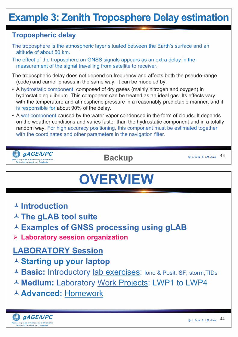
Research group of Astronomy & GeomaticsTechnical University of Catalonia
gAGE/UPC @ J. Sanz & J.M. Juan
Tropospheric delayThe troposphere is the atmospheric layer situated between the Earth’s surface and an
altitude of about 50 km. The effect of the troposphere on GNSS signals appears as an extra delay in the
measurement of the signal travelling from satellite to receiver.
The tropospheric delay does not depend on frequency and affects both the pseudo-range (code) and carrier phases in the same way. It can be modeled by:
• A hydrostatic component, composed of dry gases (mainly nitrogen and oxygen) in hydrostatic equilibrium. This component can be treated as an ideal gas. Its effects vary with the temperature and atmospheric pressure in a reasonably predictable manner, and it is responsible for about 90% of the delay.
• A wet component caused by the water vapor condensed in the form of clouds. It depends on the weather conditions and varies faster than the hydrostatic component and in a totally random way. For high accuracy positioning, this component must be estimated together with the coordinates and other parameters in the navigation filter.
Backup
Example 3: Zenith Troposphere Delay estimation
43
Research group of Astronomy & GeomaticsTechnical University of Catalonia
gAGE/UPC @ J. Sanz & J.M. Juan
IntroductionThe gLAB tool suiteExamples of GNSS processing using gLABLaboratory session organization
LABORATORY SessionStarting up your laptopBasic: Introductory lab exercises: Iono & Posit, SF, storm,TIDs
Medium: Laboratory Work Projects: LWP1 to LWP4Advanced: Homework
OVERVIEW
44
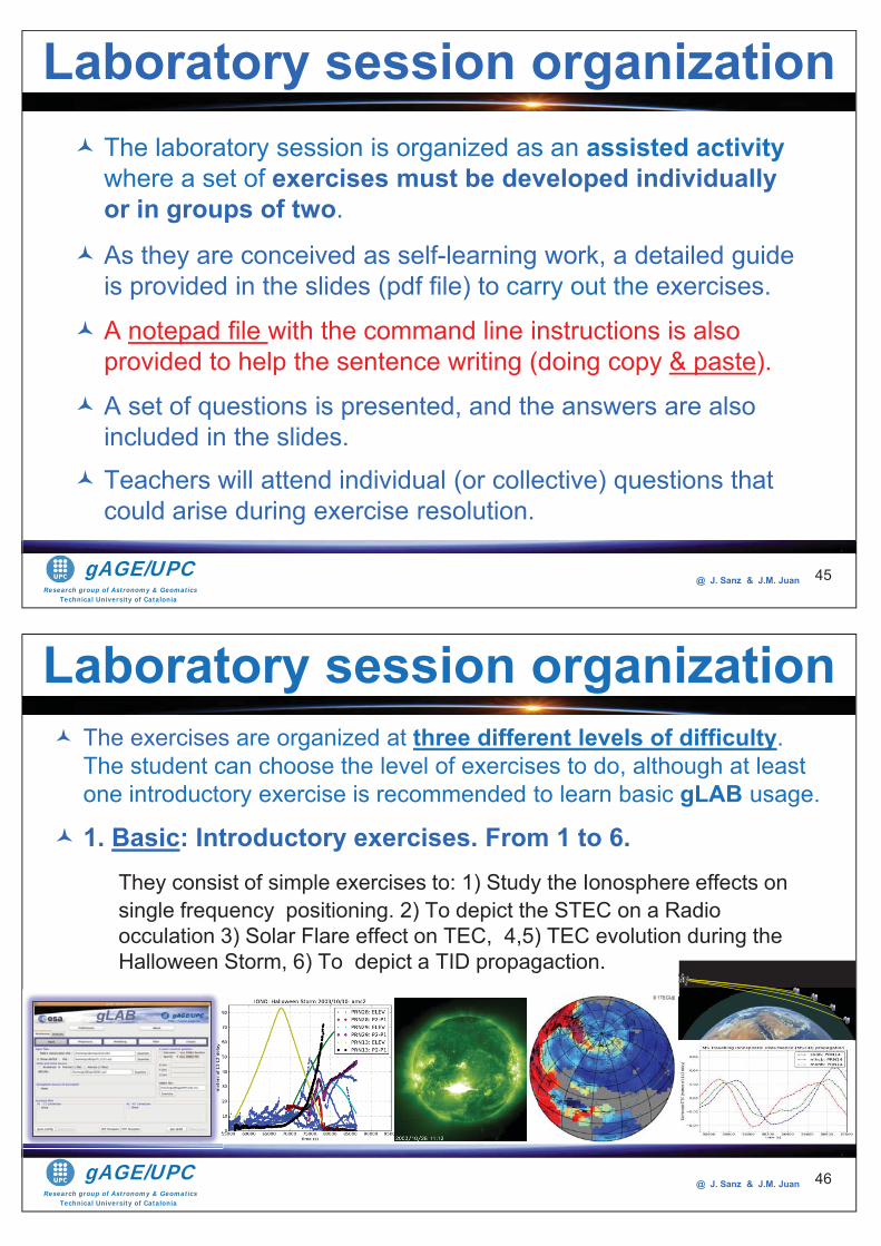
Research group of Astronomy & GeomaticsTechnical University of Catalonia
gAGE/UPC @ J. Sanz & J.M. Juan
The laboratory session is organized as an assisted activity where a set of exercises must be developed individually or in groups of two.
As they are conceived as self-learning work, a detailed guide is provided in the slides (pdf file) to carry out the exercises.
A notepad file with the command line instructions is also provided to help the sentence writing (doing copy & paste).
A set of questions is presented, and the answers are also included in the slides.Teachers will attend individual (or collective) questions that could arise during exercise resolution.
Laboratory session organization
45
Research group of Astronomy & GeomaticsTechnical University of Catalonia
gAGE/UPC @ J. Sanz & J.M. Juan
The exercises are organized at three different levels of difficulty.The student can choose the level of exercises to do, although at least one introductory exercise is recommended to learn basic gLAB usage.
1. Basic: Introductory exercises. From 1 to 6.They consist of simple exercises to: 1) Study the Ionosphere effects on single frequency positioning. 2) To depict the STEC on a Radio occulation 3) Solar Flare effect on TEC, 4,5) TEC evolution during the Halloween Storm, 6) To depict a TID propagaction.
Laboratory session organization
G Pa
46
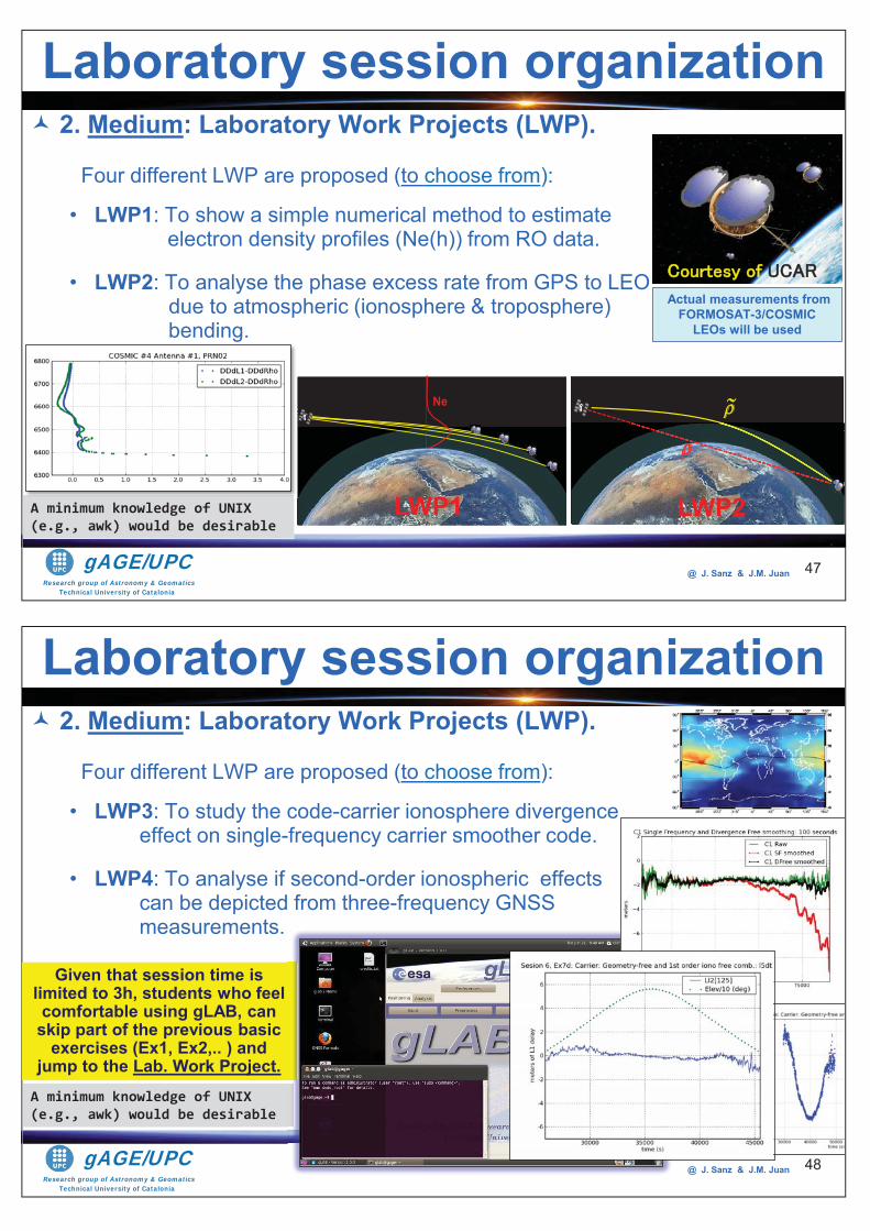
Research group of Astronomy & GeomaticsTechnical University of Catalonia
gAGE/UPC @ J. Sanz & J.M. Juan
G Pa
A minimum knowledge of UNIX (e.g., awk) would be desirable
2. Medium: Laboratory Work Projects (LWP).
Four different LWP are proposed (to choose from):
• LWP1: To show a simple numerical method to estimate electron density profiles (Ne(h)) from RO data.
• LWP2: To analyse the phase excess rate from GPS to LEO due to atmospheric (ionosphere & troposphere) bending.
Laboratory session organization
G Pa
Ne
LWP1 LWP2
Actual measurements from FORMOSAT-3/COSMIC
LEOs will be used
aa
47
Research group of Astronomy & GeomaticsTechnical University of Catalonia
gAGE/UPC @ J. Sanz & J.M. Juan
A minimum knowledge of UNIX (e.g., awk) would be desirable
Given that session time is limited to 3h, students who feel comfortable using gLAB, can
skip part of the previous basic exercises (Ex1, Ex2,.. ) and
jump to the Lab. Work Project.
2. Medium: Laboratory Work Projects (LWP).
Four different LWP are proposed (to choose from):
• LWP3: To study the code-carrier ionosphere divergence effect on single-frequency carrier smoother code.
• LWP4: To analyse if second-order ionospheric effects can be depicted from three-frequency GNSS measurements.
Laboratory session organization
f f
48
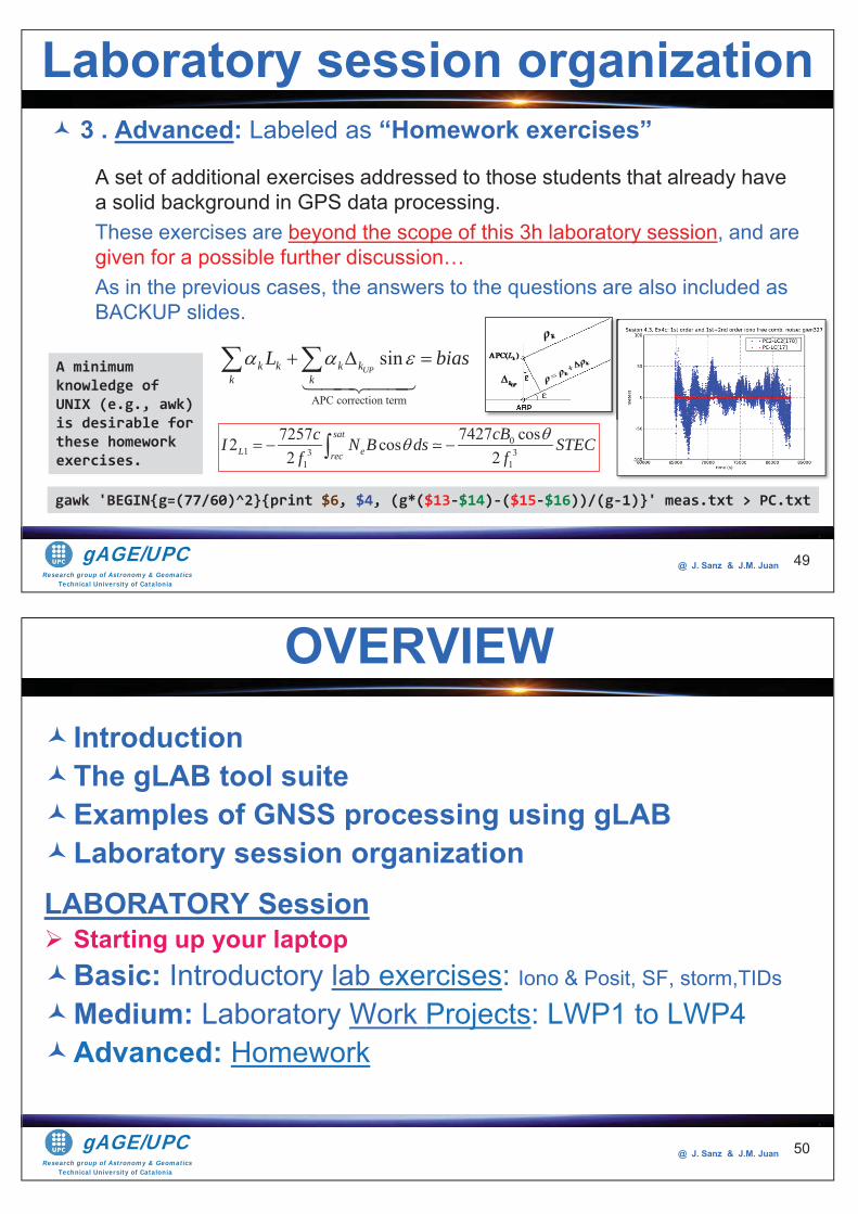
Research group of Astronomy & GeomaticsTechnical University of Catalonia
gAGE/UPC @ J. Sanz & J.M. Juan
3 . Advanced: Labeled as “Homework exercises”
A set of additional exercises addressed to those students that already have a solid background in GPS data processing.These exercises are beyond the scope of this 3h laboratory session, and are given for a possible further discussion…As in the previous cases, the answers to the questions are also included as BACKUP slides.
gawk 'BEGIN{g=(77/60)^2}{print $6, $4, (g*($13-$14)-($15-$16))/(g-1)}' meas.txt > PC.txt
A minimum knowledge of UNIX (e.g., awk) is desirable for these homework exercises.
Laboratory session organization
APC correction term
sinUPk k k k
k kL bias
01 3 3
1 1
7427 cos72572 cos2 2
sat
L erec
cBcI N B ds STECf f
49
Research group of Astronomy & GeomaticsTechnical University of Catalonia
gAGE/UPC @ J. Sanz & J.M. Juan
IntroductionThe gLAB tool suiteExamples of GNSS processing using gLABLaboratory session organization
LABORATORY SessionStarting up your laptopBasic: Introductory lab exercises: Iono & Posit, SF, storm,TIDs
Medium: Laboratory Work Projects: LWP1 to LWP4Advanced: Homework
OVERVIEW
50
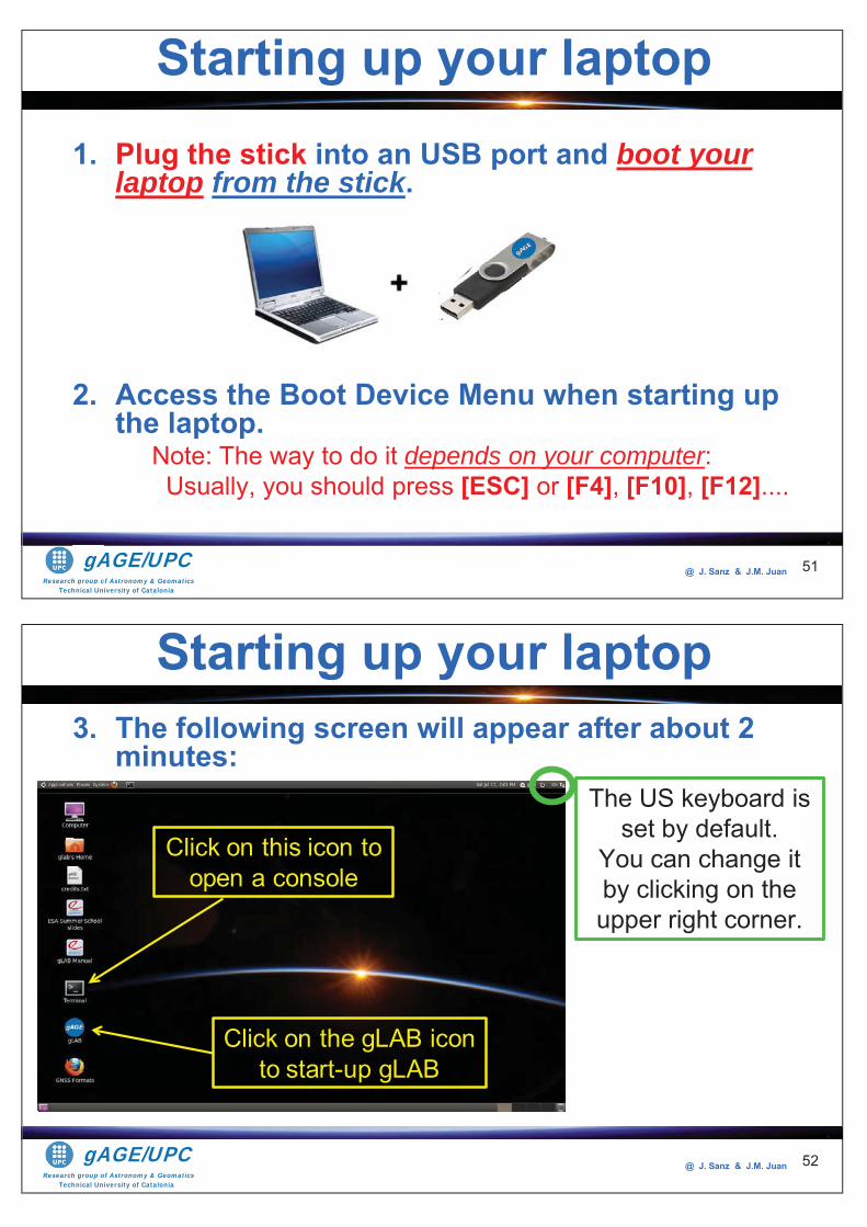
Research group of Astronomy & GeomaticsTechnical University of Catalonia
gAGE/UPC @ J. Sanz & J.M. Juan 51
1. Plug the stick into an USB port and boot your laptop from the stick.
2. Access the Boot Device Menu when starting up the laptop.
Note: The way to do it depends on your computer:Usually, you should press [ESC] or [F4], [F10], [F12]....
hh group o
gA
Starting up your laptop
Research group of Astronomy & GeomaticsTechnical University of Catalonia
gAGE/UPC @ J. Sanz & J.M. Juan
3. The following screen will appear after about 2 minutes:
52
The US keyboard is set by default.
You can change it by clicking on the upper right corner.
Click on the gLAB icon to start-up gLAB
Click on this icon to open a console
Starting up your laptop
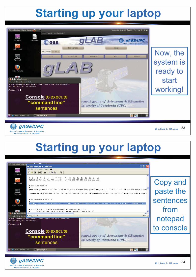
Research group of Astronomy & GeomaticsTechnical University of Catalonia
gAGE/UPC @ J. Sanz & J.M. Juan 53
Now, the system is ready to
start working!
Console to execute “command line”
sentences
Starting up your laptop
Research group of Astronomy & GeomaticsTechnical University of Catalonia
gAGE/UPC @ J. Sanz & J.M. Juan 54
Copy and paste the sentences
from notepad
to consoleConsole to execute “command line”
sentences
Starting up your laptop
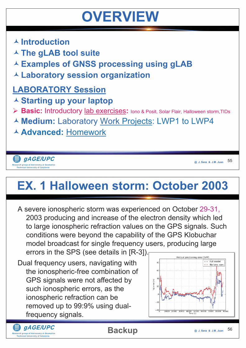
Research group of Astronomy & GeomaticsTechnical University of Catalonia
gAGE/UPC @ J. Sanz & J.M. Juan
IntroductionThe gLAB tool suiteExamples of GNSS processing using gLABLaboratory session organization
LABORATORY SessionStarting up your laptopBasic: Introductory lab exercises: Iono & Posit, Solar Flair, Halloween storm,TIDs
Medium: Laboratory Work Projects: LWP1 to LWP4Advanced: Homework
OVERVIEW
55
Research group of Astronomy & GeomaticsTechnical University of Catalonia
gAGE/UPC @ J. Sanz & J.M. Juan
A severe ionospheric storm was experienced on October 29-31,2003 producing and increase of the electron density which led to large ionospheric refraction values on the GPS signals. Such conditions were beyond the capability of the GPS Klobuchar model broadcast for single frequency users, producing large errors in the SPS (see details in [R-3]).
56
EX. 1 Halloween storm: October 2003
Dual frequency users, navigating with the ionospheric-free combination of GPS signals were not affected by such ionospheric errors, as the ionospheric refraction can be removed up to 99:9% using dual-frequency signals.
.
Backup
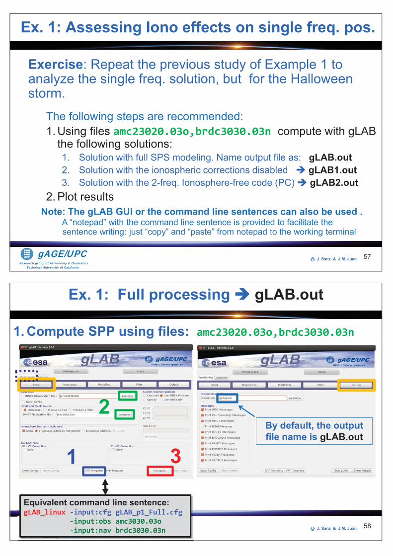
Research group of Astronomy & GeomaticsTechnical University of Catalonia
gAGE/UPC @ J. Sanz & J.M. Juan
Exercise: Repeat the previous study of Example 1 to analyze the single freq. solution, but for the Halloween storm.
The following steps are recommended:1. Using files amc23020.03o,brdc3030.03n compute with gLAB
the following solutions:1. Solution with full SPS modeling. Name output file as: gLAB.out2. Solution with the ionospheric corrections disabled gLAB1.out3. Solution with the 2-freq. Ionosphere-free code (PC) gLAB2.out
2. Plot results
57
Ex. 1: Assessing Iono effects on single freq. pos.
Note: The gLAB GUI or the command line sentences can also be used . A “notepad” with the command line sentence is provided to facilitate the sentence writing: just “copy” and “paste” from notepad to the working terminal
Research group of Astronomy & GeomaticsTechnical University of Catalonia
gAGE/UPC @ J. Sanz & J.M. Juan 58
1. Compute SPP using files: amc23020.03o,brdc3030.03n
1
2
3
Technical Unive yyrsity of CataloniaRR
TechnTechnicalicalTechnTechnicalical UniveUniversityrsityUniveUniversityrsity ofofofof CatalCataloniaoniaCatalCataloniaonia
Equivalent command line sentence:gLAB_linux -input:cfg gLAB_p1_Full.cfg -input:obs amc3030.03o -input:nav brdc3030.03n
By default, the output file name is gLAB.out
Ex. 1: Full processing gLAB.out
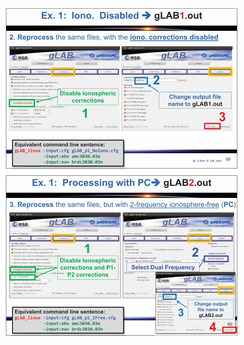
Research group of Astronomy & GeomaticsTechnical University of Catalonia
gAGE/UPC @ J. Sanz & J.M. Juan 59
Ex. 1: Iono. Disabled gLAB1.out
Change output file name to gLAB1.out
Disable Ionospheric corrections
31
2
2. Reprocess the same files, with the iono. corrections disabled
ecTechn caical U eUnive yyys yrsity oof Ca aCatalo aoniaRR
TechnTechnicalicalTechnTechnicalical UniveUniversityrsityUniveUniversityrsity ofofofof CatalCataloniaoniaCatalCataloniaonia
Equivalent command line sentence:gLAB_linux -input:cfg gLAB_p1_NoIono.cfg -input:obs amc3030.03o -input:nav brdc3030.03n
Research group of Astronomy & GeomaticsTechnical University of Catalonia
gAGE/UPC @ J. Sanz & J.M. Juan 60@@@@@@@@@ JJJ... SanSanSanzz & J.M. JuaJuaJuaJ nnn 60
3. Reprocess the same files, but with 2-frequency ionosphere-free (PC)
Ex. 1: Processing with PC gLAB2.out
Disable Ionospheric corrections and P1-
P2 corrections
1Select Dual Frequency
2
Change output file name to gLAB2.out 3
4Technical Unive yyrsity of Catalonia
RRRTechnTechnicalicalTechnical UniveUniversityrsityUniversity ofofof CatalCataloniaoniaCatalonia
Equivalent command line sentence:gLAB_linux -input:cfg gLAB_p1_IFree.cfg -input:obs amc3030.03o -input:nav brdc3030.03n
60
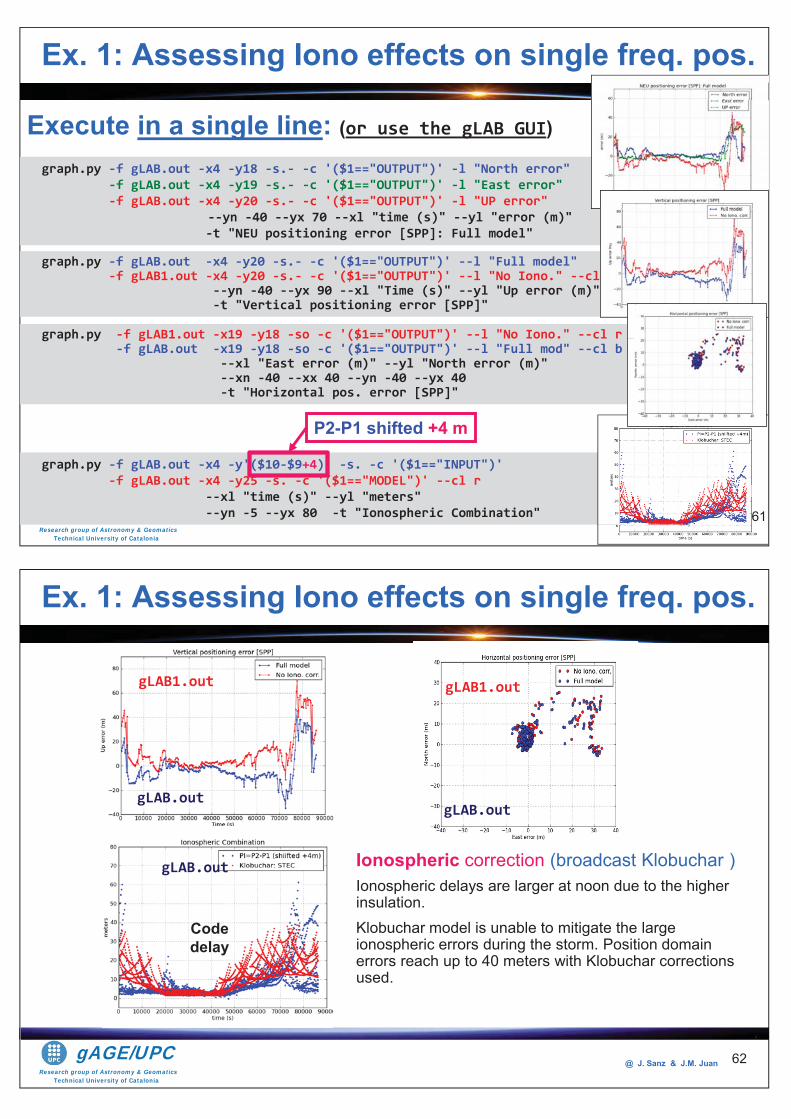
Research group of Astronomy & GeomaticsTechnical University of Catalonia
gAGE/UPC @ J. Sanz & J.M. Juan
graph.py -f gLAB.out -x4 -y18 -s.- -c '($1=="OUTPUT")' -l "North error" -f gLAB.out -x4 -y19 -s.- -c '($1=="OUTPUT")' -l "East error" -f gLAB.out -x4 -y20 -s.- -c '($1=="OUTPUT")' -l "UP error" --yn -40 --yx 70 --xl "time (s)" --yl "error (m)" -t "NEU positioning error [SPP]: Full model"
61
Execute in a single line: (or use the gLAB GUI)
graph.py -f gLAB.out -x4 -y20 -s.- -c '($1=="OUTPUT")' --l "Full model" -f gLAB1.out -x4 -y20 -s.- -c '($1=="OUTPUT")' --l "No Iono." --cl r --yn -40 --yx 90 --xl "Time (s)" --yl "Up error (m)" -t "Vertical positioning error [SPP]"
graph.py -f gLAB1.out -x19 -y18 -so -c '($1=="OUTPUT")' --l "No Iono." --cl r -f gLAB.out -x19 -y18 -so -c '($1=="OUTPUT")' --l "Full mod" --cl b --xl "East error (m)" --yl "North error (m)" --xn -40 --xx 40 --yn -40 --yx 40 -t "Horizontal pos. error [SPP]"
graph.py -f gLAB.out -x4 -y'($10-$9+4)' -s. -c '($1=="INPUT")' -f gLAB.out -x4 -y25 -s. -c '($1=="MODEL")' --cl r --xl "time (s)" --yl "meters" --yn -5 --yx 80 -t "Ionospheric Combination"
@@@@@ JJJJJJJJJJJJJJJJJJJJJJJJJJJJJJJJJJJJJJJJ... nnSannSananSaaaaSaSaSSSSannnSaSSanSanSSSanSSSSSanSSanSSSSanSSaSSaSSSanSSSaSSanSanSannSannSananSannnSanSaanSaSSSannSanSanSSaanSaSSaaSanSSSSSS nnnSaaanSSSSSS nnSanSSaanaaaaSSSSSanSannnnnanaaaaaSSSSSSSSSSSSSSSSSSSSSSSSSSSSSSSSSSSSSSSSSSSSSS zzzzzzzzzzzzzzzzzzzzzzzzzzzz &&&&&&&&&&&&&&&&&&&&&&&&&&&&&&&&&&&&&&&&&&&&&&&&&&&&&&&&&&&&&&&&&&&&&&&&&&&&&&&&&& JJJJJJJJJJJJJJJJJJJJJJJJJJJJJJJJJJJJJJJJJJJJJJJJJJJJJJJJJJJJJJJJJJJJJJJJJJJJJJJ..................MMMMMMMMMMMMMMMMMMMMMMMMMMMMMMMMMMMMMMMMMMMMMMMMMMMMMMMMMMMMMMMMMMMMMMMMMMMMMMMMMMMMMMMM..... JuauJuaJuaJuaJuaJuaJuaJuaJuJuJuJ aJJ n 616161616161616161616161616161616161616161661616161661616166161666166611111161111111111116
P2-P1 shifted +4 m
r
Ex. 1: Assessing Iono effects on single freq. pos.
61
Research group of Astronomy & GeomaticsTechnical University of Catalonia
gAGE/UPC @ J. Sanz & J.M. Juan 62
gLAB.out
gLAB1.out
gLAB.out
Code delay
gLAB.out
gLAB1.out
Ionospheric correction (broadcast Klobuchar )Ionospheric delays are larger at noon due to the higher insulation. Klobuchar model is unable to mitigate the large ionospheric errors during the storm. Position domain errors reach up to 40 meters with Klobuchar corrections used.
Ex. 1: Assessing Iono effects on single freq. pos.
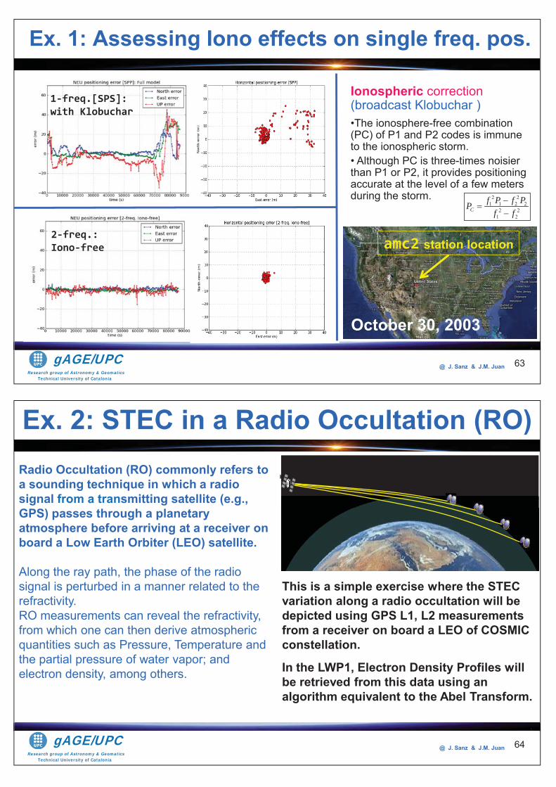
Research group of Astronomy & GeomaticsTechnical University of Catalonia
gAGE/UPC @ J. Sanz & J.M. Juan 63
2-freq.: Iono-free
1-freq.[SPS]: with Klobuchar
amc2 station location
October 30, 2003
Ionospheric correction(broadcast Klobuchar )•The ionosphere-free combination (PC) of P1 and P2 codes is immune to the ionospheric storm. • Although PC is three-times noisier than P1 or P2, it provides positioning accurate at the level of a few meters during the storm.
Ex. 1: Assessing Iono effects on single freq. pos.
2 21 1 2 2
2 21 2
Cf P f PP
f f
Research group of Astronomy & GeomaticsTechnical University of Catalonia
gAGE/UPC @ J. Sanz & J.M. Juan
Radio Occultation (RO) commonly refers to a sounding technique in which a radio signal from a transmitting satellite (e.g., GPS) passes through a planetary atmosphere before arriving at a receiver on board a Low Earth Orbiter (LEO) satellite.
Along the ray path, the phase of the radio signal is perturbed in a manner related to the refractivity.RO measurements can reveal the refractivity, from which one can then derive atmospheric quantities such as Pressure, Temperature and the partial pressure of water vapor; and electron density, among others.
Ex. 2: STEC in a Radio Occultation (RO)
This is a simple exercise where the STEC variation along a radio occultation will be depicted using GPS L1, L2 measurements from a receiver on board a LEO of COSMIC constellation.
In the LWP1, Electron Density Profiles will be retrieved from this data using an algorithm equivalent to the Abel Transform.
G Pa
64
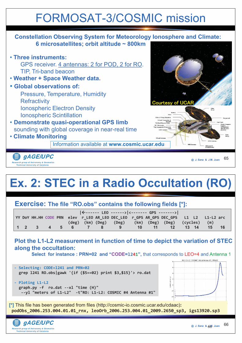
Research group of Astronomy & GeomaticsTechnical University of Catalonia
gAGE/UPC @ J. Sanz & J.M. Juan
FORMOSAT-3/COSMIC mission
65
Constellation Observing System for Meteorology Ionosphere and Climate: 6 microsatellites; orbit altitude ~ 800km
• Three instruments:GPS receiver. 4 antennas: 2 for POD, 2 for RO. TIP, Tri-band beacon
• Weather + Space Weather data. Global observations of:
Pressure, Temperature, HumidityRefractivityIonospheric Electron DensityIonospheric Scintillation
• Demonstrate quasi-operational GPS limb sounding with global coverage in near-real time
• Climate Monitoring Information available at www.cosmic.ucar.edu
Research group of Astronomy & GeomaticsTechnical University of Catalonia
gAGE/UPC @ J. Sanz & J.M. Juan 6666
Exercise: The file “RO.obs” contains the following fields [*]: | ------ LEO ------>|<------- GPS ------->| YY DoY HH.HH CODE PRN elev r_LEO AR_LEO DEC_LEO r_GPS AR_GPS DEC_GPS L1 L2 L1-L2 arc (deg) (km) (Deg) (Deg) (km) (Deg) (Deg) (cycles) (m) 1 2 3 4 5 6 7 8 9 10 11 12 13 14 15 16
Plot the L1-L2 measurement in function of time to depict the variation of STEC along the occultation: Select for instance : PRN=02 and “CODE=l241”, that corresponds to LEO=4 and Antenna 1 - Selecting: CODE=l241 and PRN=02 grep l241 RO.obs|gawk '{if ($5==02) print $3,$15}'> ro.dat - Ploting L1-L2 graph.py -f ro.dat --xl "time (H)" --yl "meters of L1-L2" -t"RO: L1-L2: COSMIC #4 Antenna #1"
Ex. 2: STEC in a Radio Occultation (RO)
p
[*] This file has been generated from files (http://cosmic-io.cosmic.ucar.edu/cdaac): podObs_2006.253.004.01.01_rnx, leoOrb_2006.253.004.01_2009.2650_sp3, igs13920.sp3
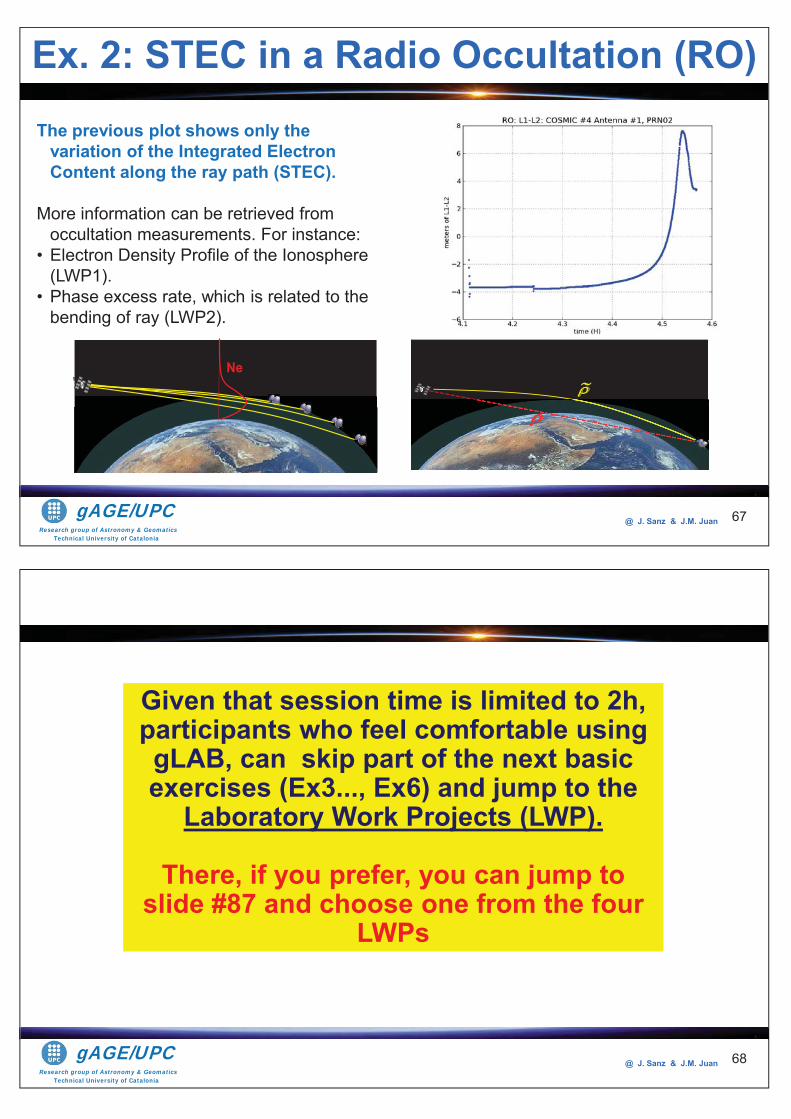
Research group of Astronomy & GeomaticsTechnical University of Catalonia
gAGE/UPC @ J. Sanz & J.M. Juan 67
The previous plot shows only the variation of the Integrated Electron Content along the ray path (STEC).
More information can be retrieved from occultation measurements. For instance:
• Electron Density Profile of the Ionosphere (LWP1).
• Phase excess rate, which is related to the bending of ray (LWP2).
G Pa
NeG P
a
Ex. 2: STEC in a Radio Occultation (RO)
Research group of Astronomy & GeomaticsTechnical University of Catalonia
gAGE/UPC @ J. Sanz & J.M. Juan 68
Given that session time is limited to 2h, participants who feel comfortable using gLAB, can skip part of the next basic exercises (Ex3..., Ex6) and jump to the
Laboratory Work Projects (LWP).
There, if you prefer, you can jump to slide #87 and choose one from the four
LWPs
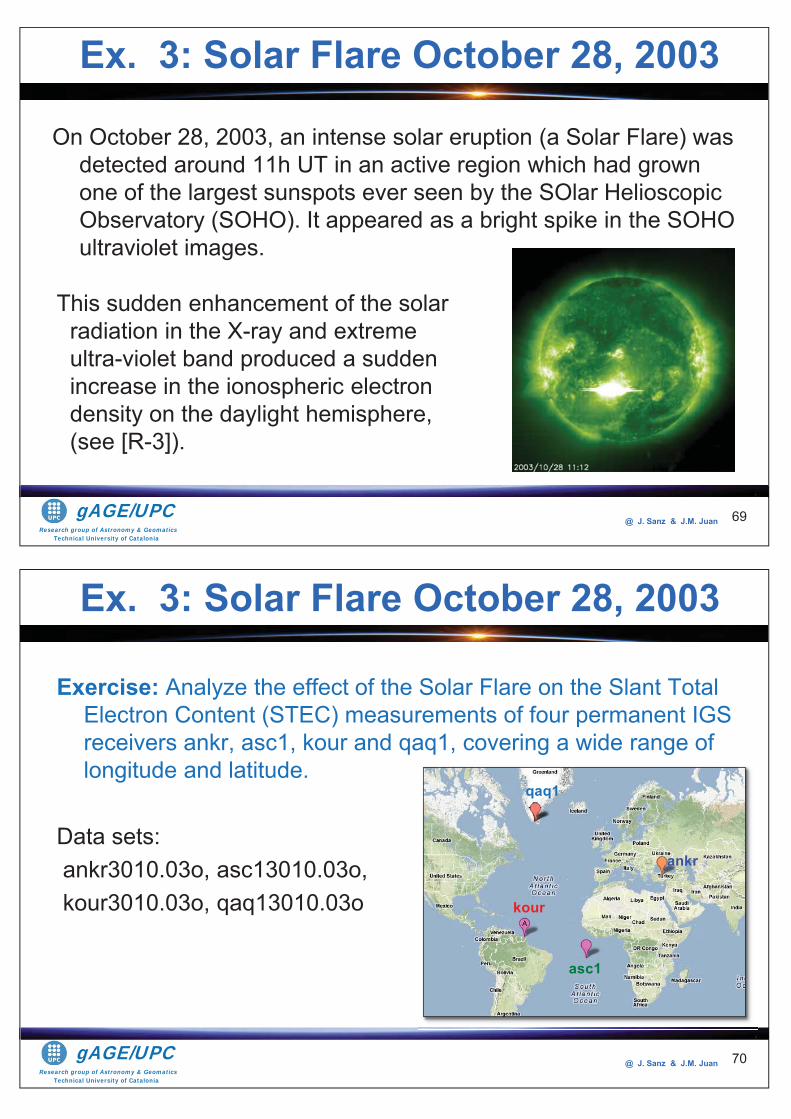
Research group of Astronomy & GeomaticsTechnical University of Catalonia
gAGE/UPC @ J. Sanz & J.M. Juan
On October 28, 2003, an intense solar eruption (a Solar Flare) was detected around 11h UT in an active region which had grown one of the largest sunspots ever seen by the SOlar Helioscopic Observatory (SOHO). It appeared as a bright spike in the SOHO ultraviolet images.
69
This sudden enhancement of the solar radiation in the X-ray and extreme ultra-violet band produced a sudden increase in the ionospheric electron density on the daylight hemisphere, (see [R-3]).
Ex. 3: Solar Flare October 28, 2003
Research group of Astronomy & GeomaticsTechnical University of Catalonia
gAGE/UPC @ J. Sanz & J.M. Juan
Exercise: Analyze the effect of the Solar Flare on the Slant Total Electron Content (STEC) measurements of four permanent IGS receivers ankr, asc1, kour and qaq1, covering a wide range of longitude and latitude.
Data sets: ankr3010.03o, asc13010.03o,kour3010.03o, qaq13010.03o
70
Ex. 3: Solar Flare October 28, 2003
ankr
qaq1
kour
asc1
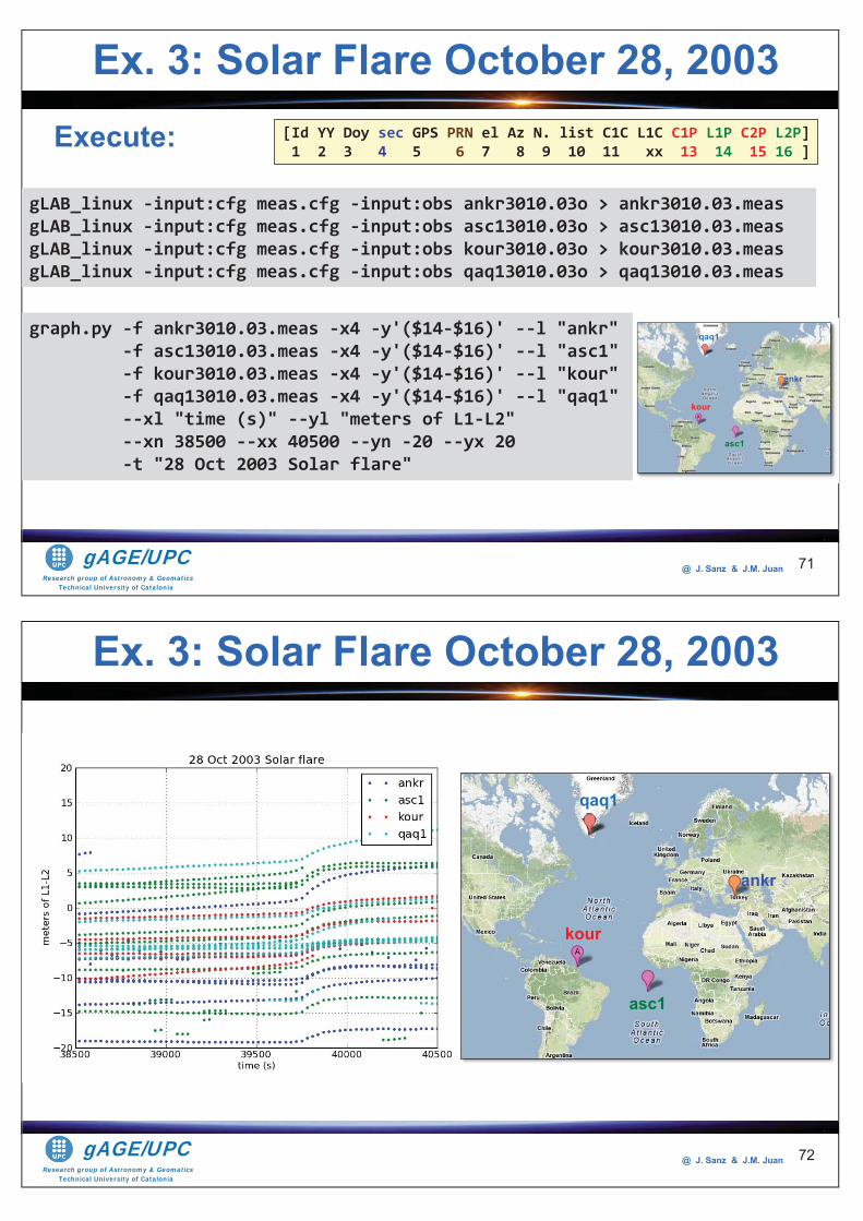
Research group of Astronomy & GeomaticsTechnical University of Catalonia
gAGE/UPC @ J. Sanz & J.M. Juan
Execute:
gLAB_linux -input:cfg meas.cfg -input:obs ankr3010.03o > ankr3010.03.meas gLAB_linux -input:cfg meas.cfg -input:obs asc13010.03o > asc13010.03.meas gLAB_linux -input:cfg meas.cfg -input:obs kour3010.03o > kour3010.03.meas gLAB_linux -input:cfg meas.cfg -input:obs qaq13010.03o > qaq13010.03.meas
graph.py -f ankr3010.03.meas -x4 -y'($14-$16)' --l "ankr" -f asc13010.03.meas -x4 -y'($14-$16)' --l "asc1" -f kour3010.03.meas -x4 -y'($14-$16)' --l "kour" -f qaq13010.03.meas -x4 -y'($14-$16)' --l "qaq1" --xl "time (s)" --yl "meters of L1-L2" --xn 38500 --xx 40500 --yn -20 --yx 20 -t "28 Oct 2003 Solar flare"
ankr
qaq1
kour
asc1
[Id YY Doy sec GPS PRN el Az N. list C1C L1C C1P L1P C2P L2P] 1 2 3 4 5 6 7 8 9 10 11 xx 13 14 15 16 ]
Ex. 3: Solar Flare October 28, 2003
71
Research group of Astronomy & GeomaticsTechnical University of Catalonia
gAGE/UPC @ J. Sanz & J.M. Juan 72
ankr
qaq1
kour
asc1
Ex. 3: Solar Flare October 28, 2003
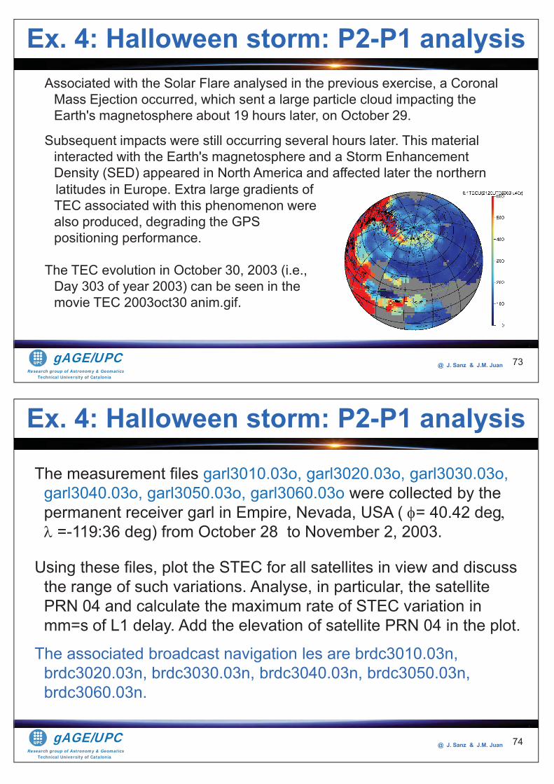
Research group of Astronomy & GeomaticsTechnical University of Catalonia
gAGE/UPC @ J. Sanz & J.M. Juan 73
Associated with the Solar Flare analysed in the previous exercise, a Coronal Mass Ejection occurred, which sent a large particle cloud impacting the Earth's magnetosphere about 19 hours later, on October 29.
Subsequent impacts were still occurring several hours later. This material interacted with the Earth's magnetosphere and a Storm Enhancement Density (SED) appeared in North America and affected later the northern
latitudes in Europe. Extra large gradients of TEC associated with this phenomenon were also produced, degrading the GPS positioning performance.
The TEC evolution in October 30, 2003 (i.e., Day 303 of year 2003) can be seen in the movie TEC 2003oct30 anim.gif.
Ex. 4: Halloween storm: P2-P1 analysis
Research group of Astronomy & GeomaticsTechnical University of Catalonia
gAGE/UPC @ J. Sanz & J.M. Juan 74
The measurement files garl3010.03o, garl3020.03o, garl3030.03o, garl3040.03o, garl3050.03o, garl3060.03o were collected by the permanent receiver garl in Empire, Nevada, USA ( = 40.42 deg
=-119:36 deg) from October 28 to November 2, 2003.
Using these files, plot the STEC for all satellites in view and discuss the range of such variations. Analyse, in particular, the satellite PRN 04 and calculate the maximum rate of STEC variation in mm=s of L1 delay. Add the elevation of satellite PRN 04 in the plot.
The associated broadcast navigation les are brdc3010.03n, brdc3020.03n, brdc3030.03n, brdc3040.03n, brdc3050.03n, brdc3060.03n.
Ex. 4: Halloween storm: P2-P1 analysis
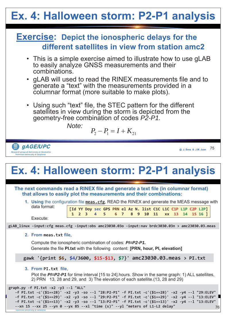
Research group of Astronomy & GeomaticsTechnical University of Catalonia
gAGE/UPC @ J. Sanz & J.M. Juan
Exercise: Depict the ionospheric delays for the different satellites in view from station amc2
• This is a simple exercise aimed to illustrate how to use gLAB to easily analyze GNSS measurements and their combinations.
• gLAB will used to read the RINEX measurements file and to generate a “text” with the measurements provided in a columnar format (more suitable to make plots).
• Using such “text” file, the STEC pattern for the different satellites in view during the storm is depicted from the geometry-free combination of codes P2-P1.
Note:
75
Ex. 4: Halloween storm: P2-P1 analysis
2 1 21P P I K
Research group of Astronomy & GeomaticsTechnical University of Catalonia
gAGE/UPC @ J. Sanz & J.M. Juan
The next commands read a RINEX file and generate a text file (in columnar format) that allows to easily plot the measurements and their combinations:
1. Using the configuration file meas.cfg, READ the RINEX and generate the MEAS message with data format:
Execute:
2. From meas.txt file, Compute the ionospheric combination of codes: PI=P2-P1.
Generate the file PI.txt with the following content: [PRN, hour, PI, elevation]
3. From PI.txt file,Plot the PI=P2-P1 for time interval [15 to 24].hours. Show in the same graph: 1) ALL satellites, 2) PRN 13, 28 and 29, and 3) The elevation of each satellite.(13, 28 and 29)
76
[Id YY Doy sec GPS PRN el Az N. list C1C L1C C1P L1P C2P L2P] 1 2 3 4 5 6 7 8 9 10 11 xx 13 14 15 16 ]
gawk '{print $6, $4/3600, $15-$13, $7}' amc23030.03.meas > PI.txt
Backup
gLAB_linux -input:cfg meas.cfg -input:obs amc23030.03o -input:nav brdc3030.03n > amc23030.03.meas
graph.py -f PI.txt -x2 -y3 --l "ALL" -f PI.txt -c'($1==28)' -x2 -y3 -so --l "28:P2-P1" -f PI.txt -c'($1==28)' -x2 -y4 --l "29:ELEV" -f PI.txt -c'($1==29)' -x2 -y3 -so --l "29:P2-P1" -f PI.txt -c'($1==29)' -x2 -y4 --l "13:ELEV" -f PI.txt -c'($1==13)' -x2 -y3 -so --l "13:P2-P1" -f PI.txt -c'($1==13)' -x2 -y4 --l "13:ELEV" --xn 15 --xx 25 --yn 0 --yx 85 --xl "time (s)" --yl "meters of L1-L2 delay"
Ex. 4: Halloween storm: P2-P1 analysis
76
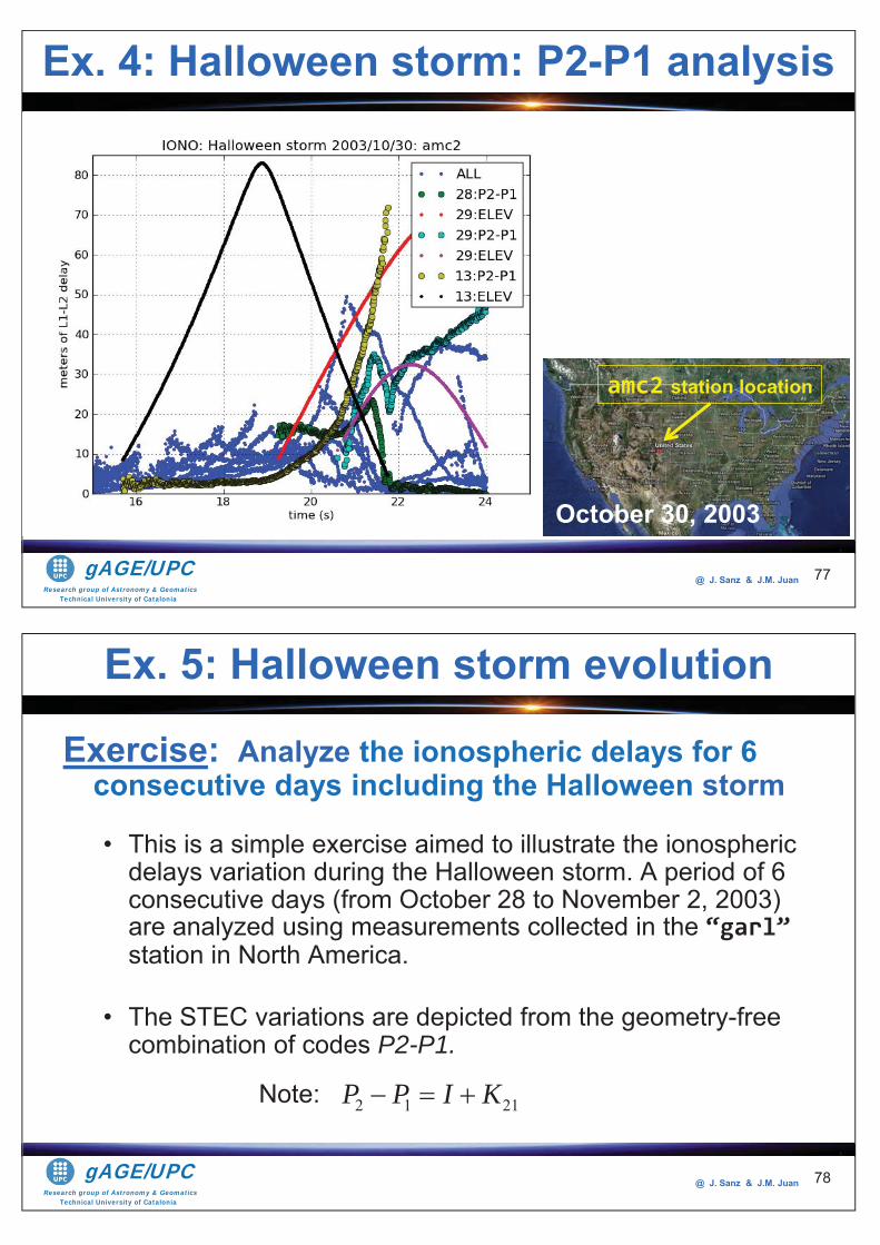
Research group of Astronomy & GeomaticsTechnical University of Catalonia
gAGE/UPC @ J. Sanz & J.M. Juan 77
Ex. 4: Halloween storm: P2-P1 analysis
amc2 station location
October 30, 2003
Research group of Astronomy & GeomaticsTechnical University of Catalonia
gAGE/UPC @ J. Sanz & J.M. Juan
Exercise: Analyze the ionospheric delays for 6 consecutive days including the Halloween storm
• This is a simple exercise aimed to illustrate the ionospheric delays variation during the Halloween storm. A period of 6 consecutive days (from October 28 to November 2, 2003) are analyzed using measurements collected in the “garl” station in North America.
• The STEC variations are depicted from the geometry-free combination of codes P2-P1.
Note:
78
Ex. 5: Halloween storm evolution
2 1 21P P I K
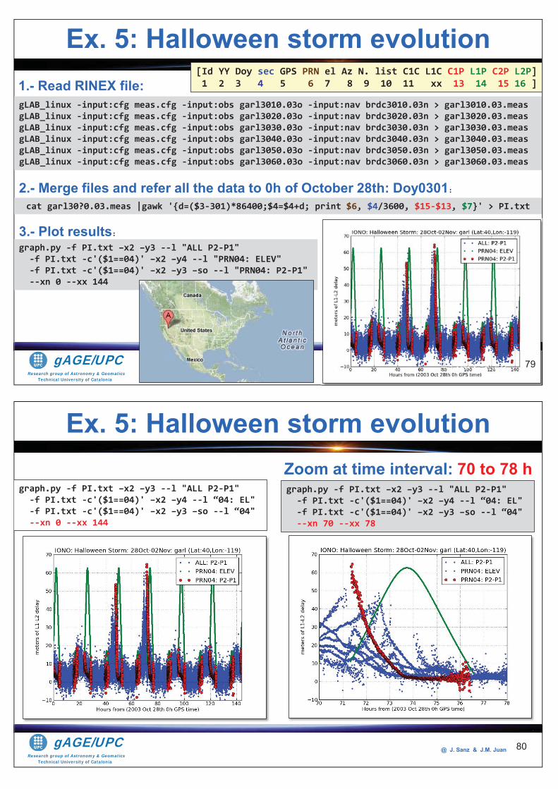
Research group of Astronomy & GeomaticsTechnical University of Catalonia
gAGE/UPC @ J. Sanz & J.M. Juan
gLAB_linux -input:cfg meas.cfg -input:obs garl3010.03o -input:nav brdc3010.03n > garl3010.03.meas gLAB_linux -input:cfg meas.cfg -input:obs garl3020.03o -input:nav brdc3020.03n > garl3020.03.meas gLAB_linux -input:cfg meas.cfg -input:obs garl3030.03o -input:nav brdc3030.03n > garl3030.03.meas gLAB_linux -input:cfg meas.cfg -input:obs garl3040.03o -input:nav brdc3040.03n > garl3040.03.meas gLAB_linux -input:cfg meas.cfg -input:obs garl3050.03o -input:nav brdc3050.03n > garl3050.03.meas gLAB_linux -input:cfg meas.cfg -input:obs garl3060.03o -input:nav brdc3060.03n > garl3060.03.meas
graph.py -f PI.txt –x2 –y3 --l "ALL P2-P1" -f PI.txt -c'($1==04)' –x2 –y4 --l "PRN04: ELEV" -f PI.txt -c'($1==04)' –x2 –y3 –so --l "PRN04: P2-P1" --xn 0 --xx 144
@@@@@@@@@@@@@@@@@@@@@@@@@@@@@@@@@@@@@@@@@@@@@@@@@@@@@@@@@@@@@@@@@@@@@@@@@@@@@@@@@@ JJJJ. SanSanSannSannnnnnnnnnnzzzzzzzzzzzzzzzzzzzzz &&&& JJJJ.MMMMMMMMMMMMMMMM....... JuaJJJJJJJJJJJJJJJJJJJJJJJJuaJuauaauJ aaaaannnnnnnnnnn
cat garl30?0.03.meas |gawk '{d=($3-301)*86400;$4=$4+d; print $6, $4/3600, $15-$13, $7}' > PI.txt
2.- Merge files and refer all the data to 0h of October 28th: Doy0301:
3.- Plot results:
1.- Read RINEX file: [Id YY Doy sec GPS PRN el Az N. list C1C L1C C1P L1P C2P L2P] 1 2 3 4 5 6 7 8 9 10 11 xx 13 14 15 16 ]
Ex. 5: Halloween storm evolution
79
Research group of Astronomy & GeomaticsTechnical University of Catalonia
gAGE/UPC @ J. Sanz & J.M. Juan
Zoom at time interval: 70 to 78 h graph.py -f PI.txt –x2 –y3 --l "ALL P2-P1" -f PI.txt -c'($1==04)' –x2 –y4 --l “04: EL" -f PI.txt -c'($1==04)' –x2 –y3 –so --l “04" --xn 0 --xx 144
graph.py -f PI.txt –x2 –y3 --l "ALL P2-P1" -f PI.txt -c'($1==04)' –x2 –y4 --l “04: EL" -f PI.txt -c'($1==04)' –x2 –y3 –so --l “04" --xn 70 --xx 78
Ex. 5: Halloween storm evolution
80
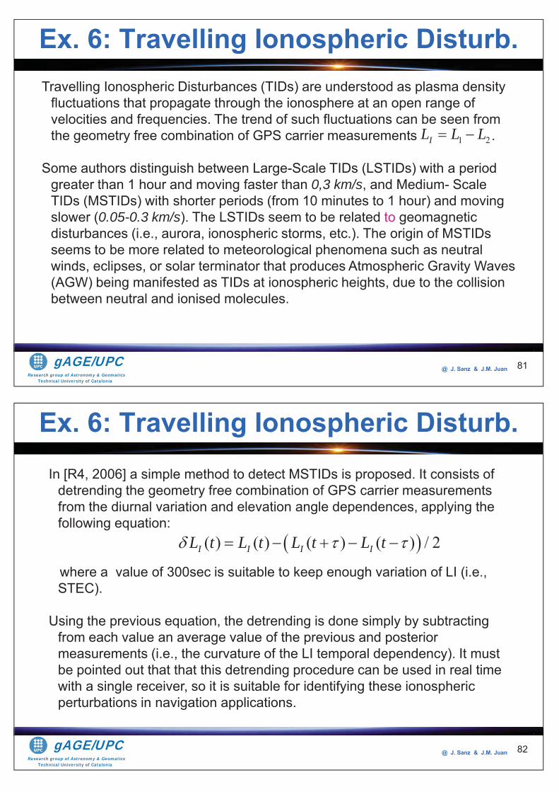
Research group of Astronomy & GeomaticsTechnical University of Catalonia
gAGE/UPC @ J. Sanz & J.M. Juan 81
Travelling Ionospheric Disturbances (TIDs) are understood as plasma density fluctuations that propagate through the ionosphere at an open range of velocities and frequencies. The trend of such fluctuations can be seen from the geometry free combination of GPS carrier measurements .
Some authors distinguish between Large-Scale TIDs (LSTIDs) with a period greater than 1 hour and moving faster than 0,3 km/s, and Medium- Scale TIDs (MSTIDs) with shorter periods (from 10 minutes to 1 hour) and moving slower (0.05-0.3 km/s). The LSTIDs seem to be related to geomagnetic disturbances (i.e., aurora, ionospheric storms, etc.). The origin of MSTIDs seems to be more related to meteorological phenomena such as neutral winds, eclipses, or solar terminator that produces Atmospheric Gravity Waves (AGW) being manifested as TIDs at ionospheric heights, due to the collision between neutral and ionised molecules.
Ex. 6: Travelling Ionospheric Disturb.
1 2IL L L
Research group of Astronomy & GeomaticsTechnical University of Catalonia
gAGE/UPC @ J. Sanz & J.M. Juan 82
In [R4, 2006] a simple method to detect MSTIDs is proposed. It consists of detrending the geometry free combination of GPS carrier measurements from the diurnal variation and elevation angle dependences, applying the following equation:
where a value of 300sec is suitable to keep enough variation of LI (i.e., STEC).
Using the previous equation, the detrending is done simply by subtracting from each value an average value of the previous and posterior measurements (i.e., the curvature of the LI temporal dependency). It must be pointed out that that this detrending procedure can be used in real time with a single receiver, so it is suitable for identifying these ionospheric perturbations in navigation applications.
Ex. 6: Travelling Ionospheric Disturb.
( ) ( ) ( ) ( ) / 2I I I IL t L t L t L t
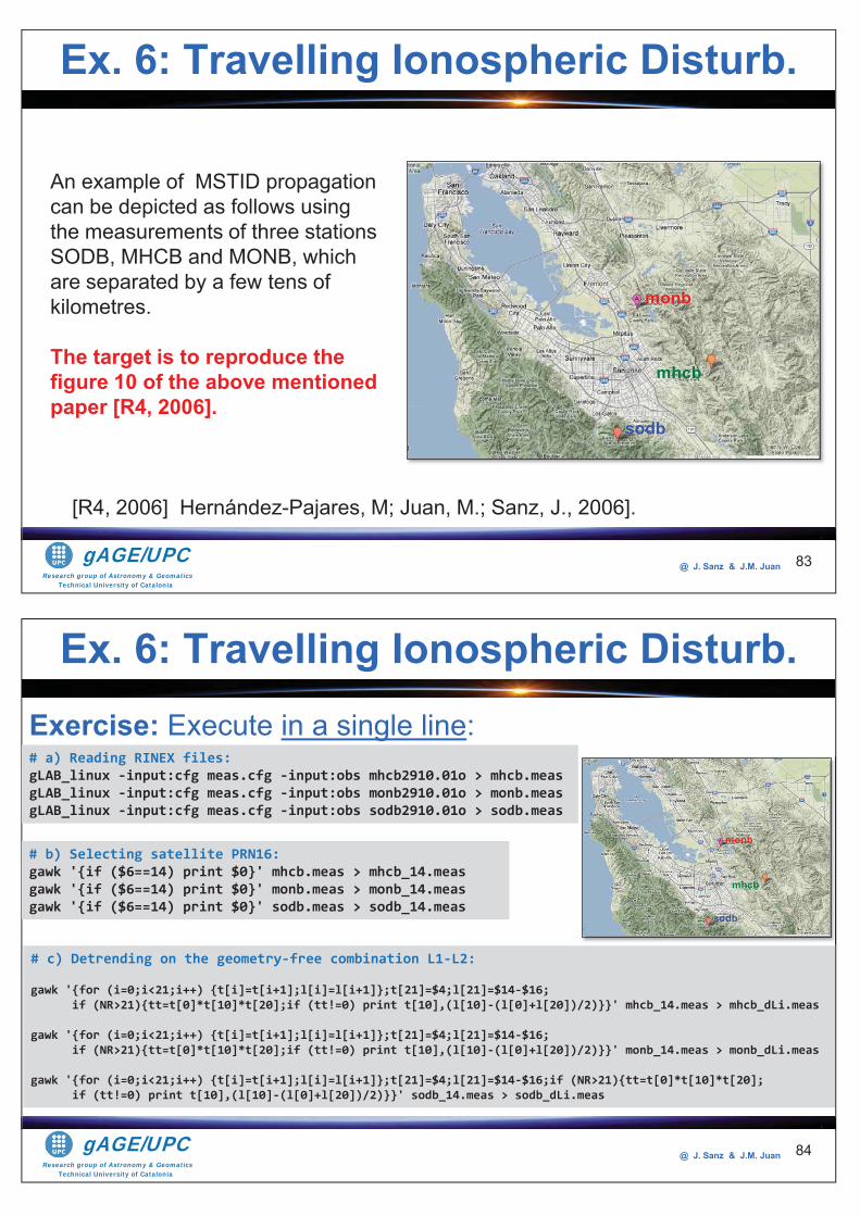
Research group of Astronomy & GeomaticsTechnical University of Catalonia
gAGE/UPC @ J. Sanz & J.M. Juan 83
An example of MSTID propagation can be depicted as follows using the measurements of three stations SODB, MHCB and MONB, which are separated by a few tens of kilometres.
The target is to reproduce the figure 10 of the above mentioned paper [R4, 2006].
Ex. 6: Travelling Ionospheric Disturb.
[R4, 2006] Hernández-Pajares, M; Juan, M.; Sanz, J., 2006].
sodb
mhcb
monb
Research group of Astronomy & GeomaticsTechnical University of Catalonia
gAGE/UPC @ J. Sanz & J.M. Juan
Exercise: Execute in a single line:# a) Reading RINEX files: gLAB_linux -input:cfg meas.cfg -input:obs mhcb2910.01o > mhcb.meas gLAB_linux -input:cfg meas.cfg -input:obs monb2910.01o > monb.meas gLAB_linux -input:cfg meas.cfg -input:obs sodb2910.01o > sodb.meas
# b) Selecting satellite PRN16: gawk '{if ($6==14) print $0}' mhcb.meas > mhcb_14.meas gawk '{if ($6==14) print $0}' monb.meas > monb_14.meas gawk '{if ($6==14) print $0}' sodb.meas > sodb_14.meas
# c) Detrending on the geometry-free combination L1-L2: gawk '{for (i=0;i<21;i++) {t[i]=t[i+1];l[i]=l[i+1]};t[21]=$4;l[21]=$14-$16; if (NR>21){tt=t[0]*t[10]*t[20];if (tt!=0) print t[10],(l[10]-(l[0]+l[20])/2)}}' mhcb_14.meas > mhcb_dLi.meas gawk '{for (i=0;i<21;i++) {t[i]=t[i+1];l[i]=l[i+1]};t[21]=$4;l[21]=$14-$16; if (NR>21){tt=t[0]*t[10]*t[20];if (tt!=0) print t[10],(l[10]-(l[0]+l[20])/2)}}' monb_14.meas > monb_dLi.meas gawk '{for (i=0;i<21;i++) {t[i]=t[i+1];l[i]=l[i+1]};t[21]=$4;l[21]=$14-$16;if (NR>21){tt=t[0]*t[10]*t[20]; if (tt!=0) print t[10],(l[10]-(l[0]+l[20])/2)}}' sodb_14.meas > sodb_dLi.meas
sodb
mhcb
monb
Ex. 6: Travelling Ionospheric Disturb.
84
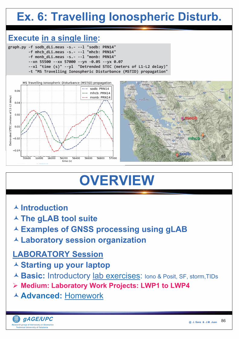
Research group of Astronomy & GeomaticsTechnical University of Catalonia
gAGE/UPC @ J. Sanz & J.M. Juan
Execute in a single line:graph.py -f sodb_dLi.meas -s.- --l "sodb: PRN14" -f mhcb_dLi.meas -s.- --l "mhcb: PRN14" -f monb_dLi.meas -s.- --l "monb: PRN14" --xn 55500 --xx 57000 --yn -0.05 --yx 0.07 --xl "time (s)" --yl "Detrended STEC (meters of L1-L2 delay)" -t "MS Travelling Ionospheric Disturbance (MSTID) propagation"
ResearchResearch group fof A tAstronomy && GeomaticsGeomaticsTechnicalTechnical UniversityUniversity ofof CataloniaCatalonia
gggggggggggggggggggggAAAAAAAAAAAAAAAAAAGGGGGEEEEEEEEEEEEE//////////////UUUUPPPPCCCCCCCCCCCCCCCCCC sodb
mhcb
monb
Ex. 6: Travelling Ionospheric Disturb.
85
Research group of Astronomy & GeomaticsTechnical University of Catalonia
gAGE/UPC @ J. Sanz & J.M. Juan
IntroductionThe gLAB tool suiteExamples of GNSS processing using gLABLaboratory session organization
LABORATORY SessionStarting up your laptopBasic: Introductory lab exercises: Iono & Posit, SF, storm,TIDsMedium: Laboratory Work Projects: LWP1 to LWP4Advanced: Homework
OVERVIEW
86
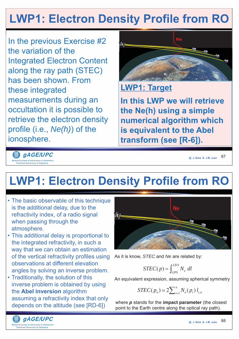
Research group of Astronomy & GeomaticsTechnical University of Catalonia
gAGE/UPC @ J. Sanz & J.M. Juan 87
In the previous Exercise #2 the variation of the Integrated Electron Content along the ray path (STEC) has been shown. From these integrated measurements during an occultation it is possible to retrieve the electron density profile (i.e., Ne(h)) of the ionosphere.
LWP1: Electron Density Profile from ROG P
aNe
LWP1: TargetIn this LWP we will retrieve the Ne(h) using a simple numerical algorithm which is equivalent to the Abel transform (see [R-6]).
Research group of Astronomy & GeomaticsTechnical University of Catalonia
gAGE/UPC @ J. Sanz & J.M. Juan 88
• The basic observable of this technique is the additional delay, due to the refractivity index, of a radio signal when passing through the atmosphere.
• This additional delay is proportional to the integrated refractivity, in such a way that we can obtain an estimation of the vertical refractivity profiles using observations at different elevation angles by solving an inverse problem.
• Traditionally, the solution of this inverse problem is obtained by using the Abel inversion algorithm assuming a refractivity index that only depends on the altitude (see [RD-6])
LWP1: Electron Density Profile from RO
G Pa
Ne
An equivalent expression, assuming spherical symmetry
where p stands for the impact parameter (the closest point to the Earth centre along the optical ray path).
As it is know, STEC and Ne are related by:
( )LEO
eGPSSTEC p N dl
,1( ) 2 ( )n
n e i i niSTEC p N p l
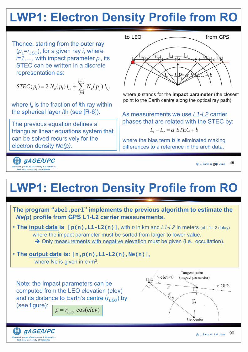
Research group of Astronomy & GeomaticsTechnical University of Catalonia
gAGE/UPC @ J. Sanz & J.M. Juan 8989
LWP1: Electron Density Profile from RO
where p stands for the impact parameter (the closest point to the Earth centre along the optical ray path).
Thence, starting from the outer ray (p1=rLEO), for a given ray i, where i=1,…, with impact parameter pi, its STEC can be written in a discrete representation as:
where lii is the fraction of ith ray within the spherical layer ith (see [R-6]).
The previous equation defines a triangular linear equations system that can be solved recursively for the electron density Ne(p).
As measurements we use L1-L2 carrier phases that are related with the STEC by:
where the bias term b is eliminated making differences to a reference in the arch data.
1
, ,1
( ) 2 ( ) ( )j i
i e i i i e j i jj
STEC p N p l N p l
1 2L L STEC b
1 2L L STEC b
Research group of Astronomy & GeomaticsTechnical University of Catalonia
gAGE/UPC @ J. Sanz & J.M. Juan 90
The program “abel.perl” implements the previous algorithm to estimate the Ne(p) profile from GPS L1-L2 carrier measurements.• The input data is [p(n),L1-L2(n)], with p in km and L1-L2 in meters (of L1-L2 delay)
where the impact parameter must be sorted from larger to lower value.Only measurements with negative elevation must be given (i.e., occultation).
• The output data is: [n,p(n),L1-L2(n),Ne(n)], where Ne is given in e-/m3.
LWP1: Electron Density Profile from RO
Note: the Impact parameters can be computed from the LEO elevation (elev) and its distance to Earth’s centre (rLEO) by (see figure):
cos( )LEOp r elev
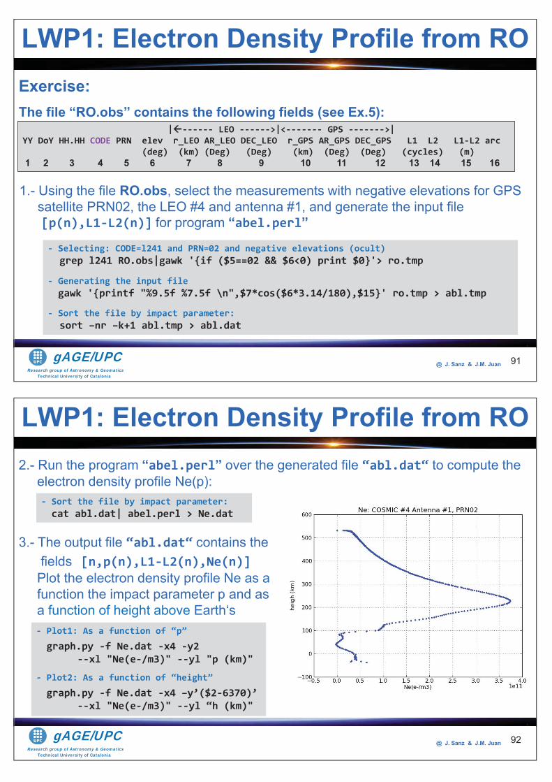
Research group of Astronomy & GeomaticsTechnical University of Catalonia
gAGE/UPC @ J. Sanz & J.M. Juan 91
- Selecting: CODE=l241 and PRN=02 and negative elevations (ocult) grep l241 RO.obs|gawk '{if ($5==02 && $6<0) print $0}'> ro.tmp
- Generating the input file gawk '{printf "%9.5f %7.5f \n",$7*cos($6*3.14/180),$15}' ro.tmp > abl.tmp
- Sort the file by impact parameter: sort –nr –k+1 abl.tmp > abl.dat
LWP1: Electron Density Profile from RO
1.- Using the file RO.obs, select the measurements with negative elevations for GPS satellite PRN02, the LEO #4 and antenna #1, and generate the input file [p(n),L1-L2(n)] for program “abel.perl”
Exercise: The file “RO.obs” contains the following fields (see Ex.5): | ------ LEO ------>|<------- GPS ------->| YY DoY HH.HH CODE PRN elev r_LEO AR_LEO DEC_LEO r_GPS AR_GPS DEC_GPS L1 L2 L1-L2 arc (deg) (km) (Deg) (Deg) (km) (Deg) (Deg) (cycles) (m) 1 2 3 4 5 6 7 8 9 10 11 12 13 14 15 16
Research group of Astronomy & GeomaticsTechnical University of Catalonia
gAGE/UPC @ J. Sanz & J.M. Juan 92
- Sort the file by impact parameter: cat abl.dat| abel.perl > Ne.dat
LWP1: Electron Density Profile from RO2.- Run the program “abel.perl” over the generated file “abl.dat“ to compute the electron density profile Ne(p):
3.- The output file “abl.dat“ contains the fields [n,p(n),L1-L2(n),Ne(n)] Plot the electron density profile Ne as a function the impact parameter p and as a function of height above Earth‘s
- Plot1: As a function of “p”
graph.py -f Ne.dat -x4 -y2 --xl "Ne(e-/m3)" --yl "p (km)"
- Plot2: As a function of “height”
graph.py -f Ne.dat -x4 –y’($2-6370)’ --xl "Ne(e-/m3)" --yl “h (km)"
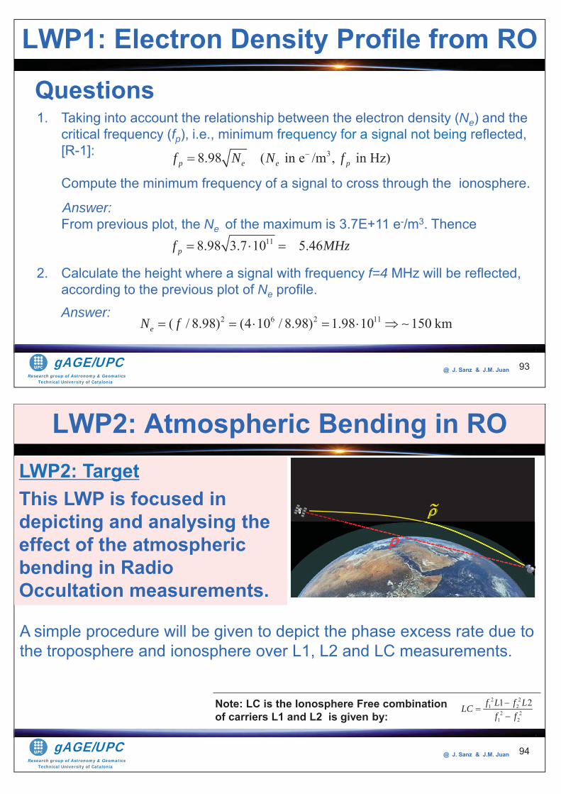
Research group of Astronomy & GeomaticsTechnical University of Catalonia
gAGE/UPC @ J. Sanz & J.M. Juan 93
LWP1: Electron Density Profile from RO
1. Taking into account the relationship between the electron density (Ne) and the critical frequency (fp), i.e., minimum frequency for a signal not being reflected, [R-1]:
Compute the minimum frequency of a signal to cross through the ionosphere.
Answer: From previous plot, the Ne of the maximum is 3.7E+11 e-/m3. Thence
2. Calculate the height where a signal with frequency f=4 MHz will be reflected, according to the previous plot of Ne profile.Answer:
38.98 ( in e /m , in Hz)p e e pf N N f
Questions
118.98 3.7 10 5.46pf MHz
2 6 2 11( / 8.98) (4 10 / 8.98) 1.98 10 150 kmeN f
Research group of Astronomy & GeomaticsTechnical University of Catalonia
gAGE/UPC @ J. Sanz & J.M. Juan 94
LWP2: Atmospheric Bending in ROLWP2: TargetThis LWP is focused in depicting and analysing the effect of the atmospheric bending in Radio Occultation measurements.
A simple procedure will be given to depict the phase excess rate due to the troposphere and ionosphere over L1, L2 and LC measurements.
2 21 2
2 21 2
1 2f L f LLCf f
Note: LC is the Ionosphere Free combination of carriers L1 and L2 is given by:
G Pa
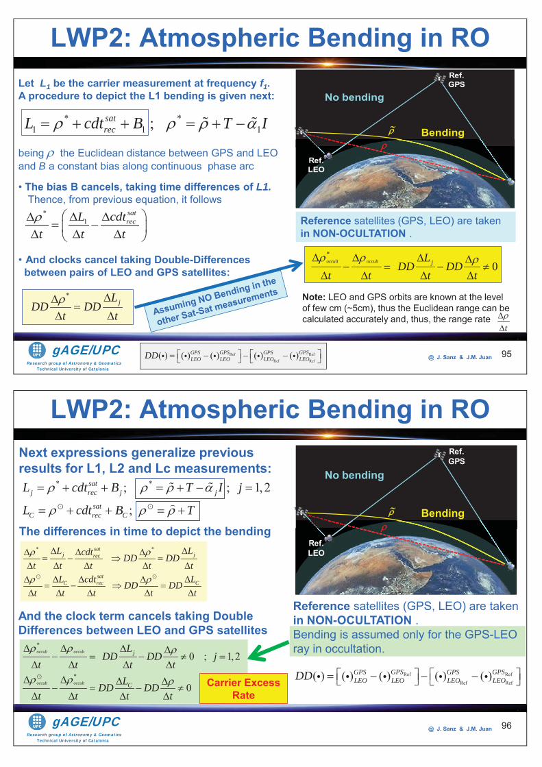
Research group of Astronomy & GeomaticsTechnical University of Catalonia
gAGE/UPC @ J. Sanz & J.M. Juan 95
LWP2: Atmospheric Bending in RO
being the Euclidean distance between GPS and LEO and B a constant bias along continuous phase arc
• The bias B cancels, taking time differences of L1.Thence, from previous equation, it follows
Let L1 be the carrier measurement at frequency f1.A procedure to depict the L1 bending is given next:
G Pa
G Pa
No bending
Bending
Ref. GPS
Ref. LEO
Ref Ref
Ref Ref( ) ( ) ( ) ( ) ( )GPS GPSGPS GPS
LEO LEO LEO LEODD
Reference satellites (GPS, LEO) are taken in NON-OCULTATION .
*jL
DD DDt t
* *1 1 1;sat
recL cdt B T I
• And clocks cancel taking Double-Differences between pairs of LEO and GPS satellites:
*1
satreccdtL
t t t
Note: LEO and GPS orbits are known at the level of few cm (~5cm), thus the Euclidean range can be calculated accurately and, thus, the range rate
t
*
0occult occult jLDD DD
t t t t
Research group of Astronomy & GeomaticsTechnical University of Catalonia
gAGE/UPC @ J. Sanz & J.M. Juan 96
LWP2: Atmospheric Bending in RO
* *satj jrec
satC rec C
L Lcdt DD DDt t t t t
L cdt LDD DDt t t t t
*
*
0 ; 1, 2
0
occult occult
occult occult
j
C
LDD DD j
t t t tLDD DD
t t t t
G Pa
G Pa
No bending
Bending
Ref. GPS
Ref. LEO
Ref Ref
Ref Ref( ) ( ) ( ) ( ) ( )GPS GPSGPS GPS
LEO LEO LEO LEODD
And the clock term cancels taking Double Differences between LEO and GPS satellites
Reference satellites (GPS, LEO) are taken in NON-OCULTATION .Bending is assumed only for the GPS-LEO ray in occultation.
* *; ; 1, 2
;
satj rec j j
satC rec C
L cdt B T I j
L cdt B T
Next expressions generalize previous results for L1, L2 and Lc measurements:
The differences in time to depict the bending
Carrier Excess Rate
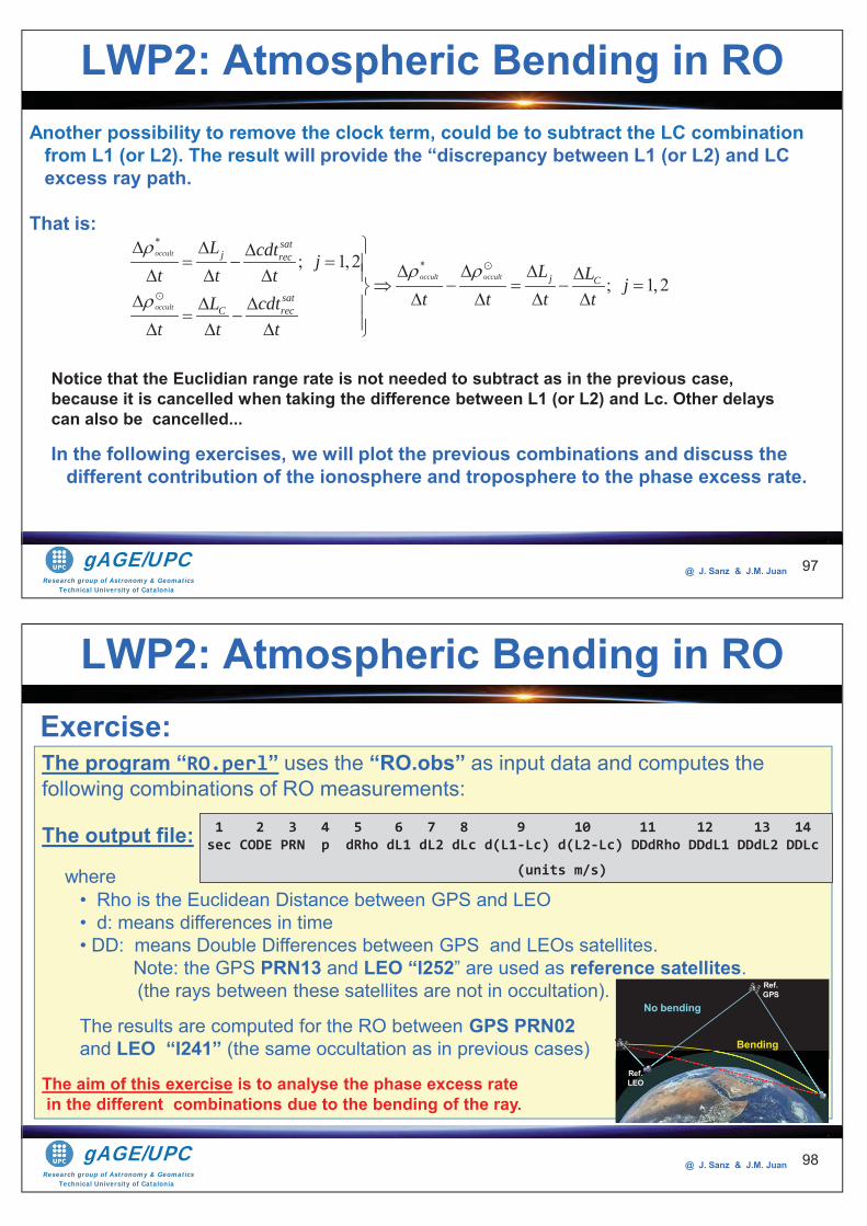
Research group of Astronomy & GeomaticsTechnical University of Catalonia
gAGE/UPC @ J. Sanz & J.M. Juan 97
LWP2: Atmospheric Bending in ROAnother possibility to remove the clock term, could be to subtract the LC combination
from L1 (or L2). The result will provide the “discrepancy between L1 (or L2) and LC excess ray path.
That is:
Notice that the Euclidian range rate is not needed to subtract as in the previous case, because it is cancelled when taking the difference between L1 (or L2) and Lc. Other delays can also be cancelled...
*
*; 1, 2; 1, 2
occult
occult occult
occult
satj rec
j Csat
C rec
L cdt j L Lt t t jt t t tL cdt
t t t
In the following exercises, we will plot the previous combinations and discuss the different contribution of the ionosphere and troposphere to the phase excess rate.
Research group of Astronomy & GeomaticsTechnical University of Catalonia
gAGE/UPC @ J. Sanz & J.M. Juan 98
The program “RO.perl” uses the “RO.obs” as input data and computes the following combinations of RO measurements:
The output file:
where • Rho is the Euclidean Distance between GPS and LEO • d: means differences in time • DD: means Double Differences between GPS and LEOs satellites.
Note: the GPS PRN13 and LEO “l252” are used as reference satellites. (the rays between these satellites are not in occultation).
The results are computed for the RO between GPS PRN02and LEO “l241” (the same occultation as in previous cases)
The aim of this exercise is to analyse the phase excess ratein the different combinations due to the bending of the ray.
LWP2: Atmospheric Bending in RO
1 2 3 4 5 6 7 8 9 10 11 12 13 14 sec CODE PRN p dRho dL1 dL2 dLc d(L1-Lc) d(L2-Lc) DDdRho DDdL1 DDdL2 DDLc
(units m/s)
G Pa
G Pa
No bending
Bending
Ref. GPS
Ref. LEO
Exercise:
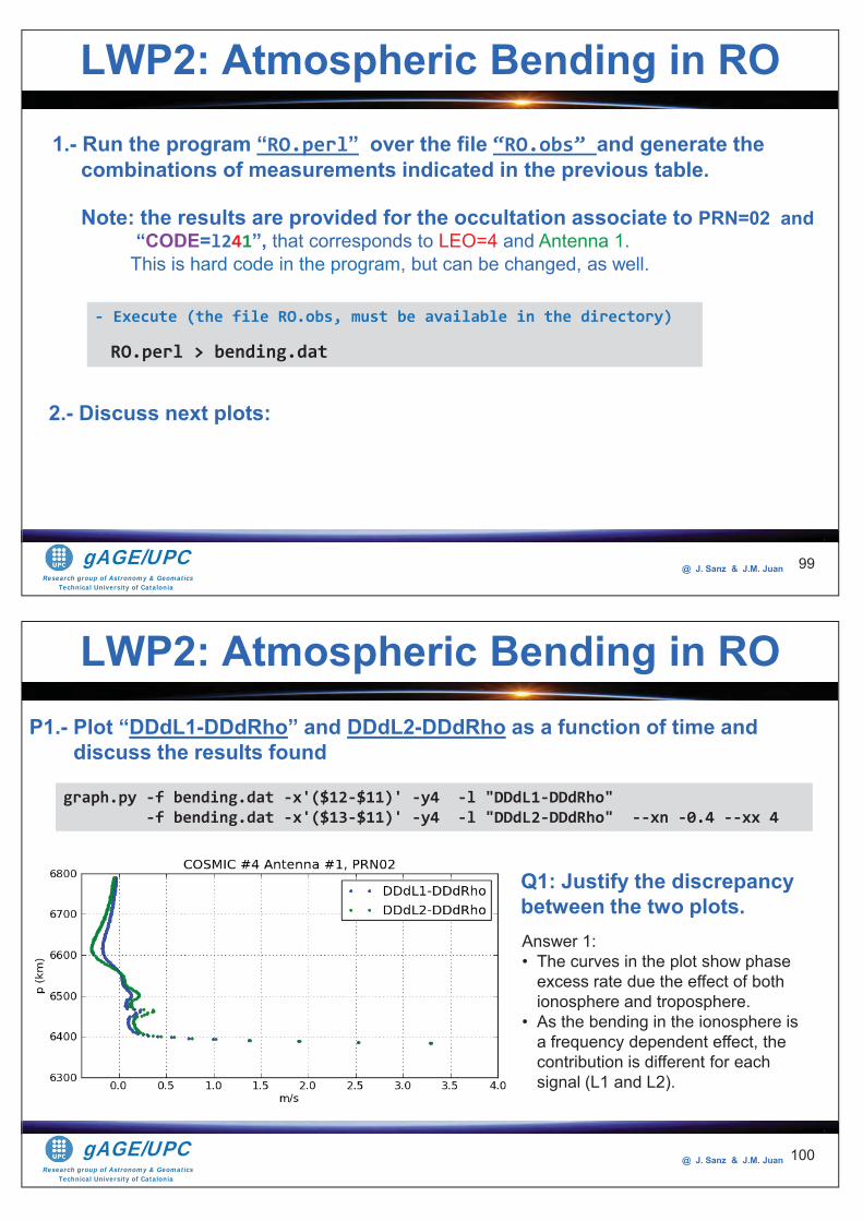
Research group of Astronomy & GeomaticsTechnical University of Catalonia
gAGE/UPC @ J. Sanz & J.M. Juan 99
1.- Run the program “RO.perl” over the file “RO.obs” and generate the combinations of measurements indicated in the previous table.
Note: the results are provided for the occultation associate to PRN=02 and “CODE=l241”, that corresponds to LEO=4 and Antenna 1. This is hard code in the program, but can be changed, as well.
- Execute (the file RO.obs, must be available in the directory)
RO.perl > bending.dat
LWP2: Atmospheric Bending in RO
2.- Discuss next plots:
Research group of Astronomy & GeomaticsTechnical University of Catalonia
gAGE/UPC @ J. Sanz & J.M. Juan 100
graph.py -f bending.dat -x'($12-$11)' -y4 -l "DDdL1-DDdRho" -f bending.dat -x'($13-$11)' -y4 -l "DDdL2-DDdRho" --xn -0.4 --xx 4
LWP2: Atmospheric Bending in ROP1.- Plot “DDdL1-DDdRho” and DDdL2-DDdRho as a function of time and
discuss the results found
Q1: Justify the discrepancy between the two plots. Answer 1: • The curves in the plot show phase
excess rate due the effect of both ionosphere and troposphere.
• As the bending in the ionosphere is a frequency dependent effect, the contribution is different for each signal (L1 and L2).
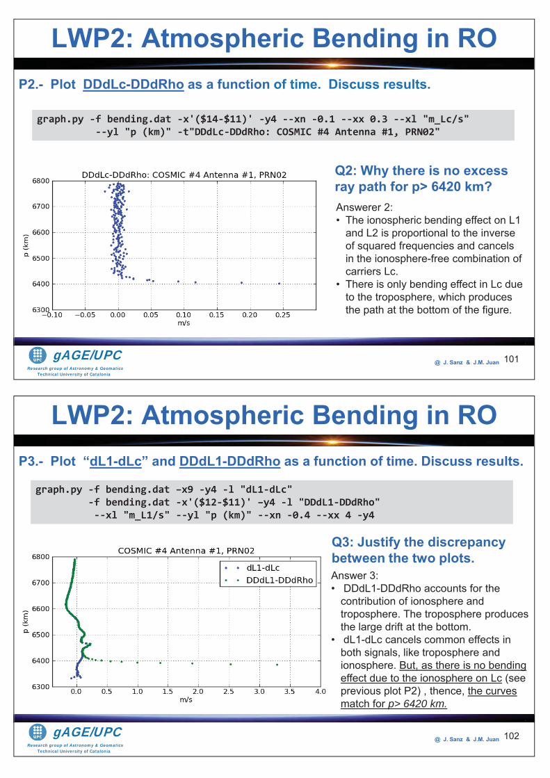
Research group of Astronomy & GeomaticsTechnical University of Catalonia
gAGE/UPC @ J. Sanz & J.M. Juan 101
graph.py -f bending.dat -x'($14-$11)' -y4 --xn -0.1 --xx 0.3 --xl "m_Lc/s" --yl "p (km)" -t"DDdLc-DDdRho: COSMIC #4 Antenna #1, PRN02"
LWP2: Atmospheric Bending in ROP2.- Plot DDdLc-DDdRho as a function of time. Discuss results.
Q2: Why there is no excess ray path for p> 6420 km?Answerer 2: • The ionospheric bending effect on L1
and L2 is proportional to the inverse of squared frequencies and cancels in the ionosphere-free combination of carriers Lc.
• There is only bending effect in Lc dueto the troposphere, which produces the path at the bottom of the figure.
Research group of Astronomy & GeomaticsTechnical University of Catalonia
gAGE/UPC @ J. Sanz & J.M. Juan 102
LWP2: Atmospheric Bending in ROP3.- Plot “dL1-dLc” and DDdL1-DDdRho as a function of time. Discuss results.
graph.py -f bending.dat –x9 -y4 -l "dL1-dLc" -f bending.dat -x'($12-$11)' –y4 -l "DDdL1-DDdRho" --xl "m_L1/s" --yl "p (km)" --xn -0.4 --xx 4 -y4
Q3: Justify the discrepancy between the two plots. Answer 3: • DDdL1-DDdRho accounts for the
contribution of ionosphere and troposphere. The troposphere produces the large drift at the bottom.
• dL1-dLc cancels common effects in both signals, like troposphere and ionosphere. But, as there is no bending effect due to the ionosphere on Lc (see previous plot P2) , thence, the curves match for p> 6420 km.
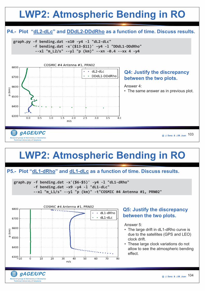
Research group of Astronomy & GeomaticsTechnical University of Catalonia
gAGE/UPC @ J. Sanz & J.M. Juan 103
LWP2: Atmospheric Bending in RO
graph.py -f bending.dat –x10 -y4 -l "dL2-dLc" -f bending.dat -x'($13-$11)' –y4 -l "DDdL1-DDdRho" --xl "m_L2/s" --yl "p (km)" --xn -0.4 --xx 4 -y4
Q4: Justify the discrepancy between the two plots. Answer 4:• The same answer as in previous plot.
P4.- Plot “dL2-dLc” and DDdL2-DDdRho as a function of time. Discuss results.
Research group of Astronomy & GeomaticsTechnical University of Catalonia
gAGE/UPC @ J. Sanz & J.M. Juan 104
LWP2: Atmospheric Bending in RO
graph.py -f bending.dat -x'($6-$5)' -y4 -l "dL1-dRho" -f bending.dat –x9 -y4 -l "dL1-dLc" --xl "m_L1/s" --yl "p (km)" -t"COSMIC #4 Antenna #1, PRN02"
P5.- Plot “dL1-dRho” and dL1-dLc as a function of time. Discuss results.
Q5: Justify the discrepancy between the two plots. Answer 5: • The large drift in dL1-dRho curve is
due to the satellites (GPS and LEO) clock drift.
• These large clock variations do not allow to see the atmospheric bending effect.
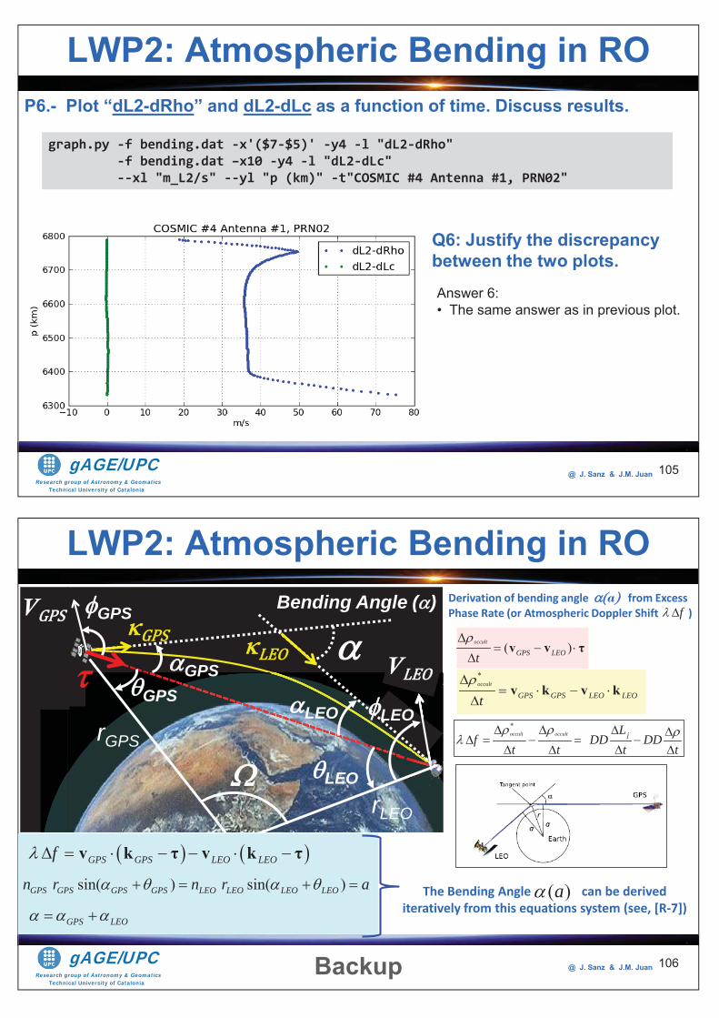
Research group of Astronomy & GeomaticsTechnical University of Catalonia
gAGE/UPC @ J. Sanz & J.M. Juan 105
LWP2: Atmospheric Bending in RO
graph.py -f bending.dat -x'($7-$5)' -y4 -l "dL2-dRho" -f bending.dat –x10 -y4 -l "dL2-dLc" --xl "m_L2/s" --yl "p (km)" -t"COSMIC #4 Antenna #1, PRN02"
P6.- Plot “dL2-dRho” and dL2-dLc as a function of time. Discuss results.
Q6: Justify the discrepancy between the two plots. Answer 6: • The same answer as in previous plot.
Research group of Astronomy & GeomaticsTechnical University of Catalonia
gAGE/UPC @ J. Sanz & J.M. Juan
vGPS vLEOGPS LEOG P
a LLLLLLEEEEEEEEEOOOOOOGPPPPPPPPPPPSSSSSS OGPS
LEO
Bending Angle ( )
rGPS
rLEO
LWP2: Atmospheric Bending in RO
Backup
GPS VGPS LEO VLEO GPS
GPS
LEOLEO
*occult occult jL
f DD DDt t t t
Derivation of bending angle a from Excess Phase Rate (or Atmospheric Doppler Shift )
( )occult
GPS LEOtv v
*occult
GPS GPS LEO LEOtv k v k
sin( ) sin( )GPS GPS GPS GPS LEO LEO LEO LEOn r n r a
GPS GPS LEO LEOf v k
GPS LEO
( )aThe Bending Angle can be derived iteratively from this equations system (see, [R-7])
f
106
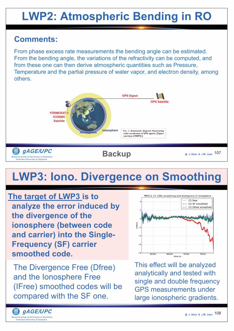
Research group of Astronomy & GeomaticsTechnical University of Catalonia
gAGE/UPC @ J. Sanz & J.M. Juan 107
LWP2: Atmospheric Bending in RO
Comments:From phase excess rate measurements the bending angle can be estimated.From the bending angle, the variations of the refractivity can be computed, and from these one can then derive atmospheric quantities such as Pressure, Temperature and the partial pressure of water vapor, and electron density, among others.
Backup
Research group of Astronomy & GeomaticsTechnical University of Catalonia
gAGE/UPC @ J. Sanz & J.M. Juan 108
The target of LWP3 is to analyze the error induced by the divergence of the ionosphere (between code and carrier) into the Single-Frequency (SF) carrier smoothed code.
LWP3: Iono. Divergence on Smoothing
This effect will be analyzed analytically and tested with single and double frequency GPS measurements under large ionospheric gradients.
The Divergence Free (Dfree) and the Ionosphere Free (IFree) smoothed codes will be compared with the SF one.
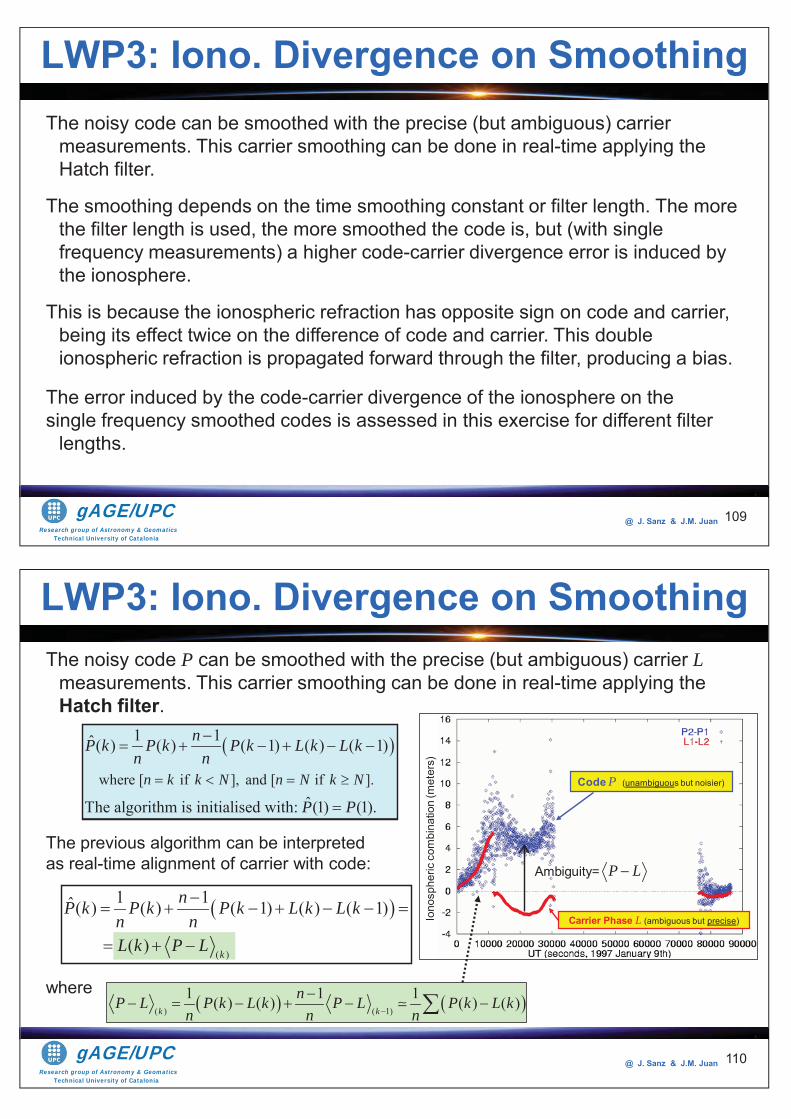
Research group of Astronomy & GeomaticsTechnical University of Catalonia
gAGE/UPC @ J. Sanz & J.M. Juan 109
The noisy code can be smoothed with the precise (but ambiguous) carrier measurements. This carrier smoothing can be done in real-time applying the Hatch filter.
The smoothing depends on the time smoothing constant or filter length. The more the filter length is used, the more smoothed the code is, but (with single frequency measurements) a higher code-carrier divergence error is induced by the ionosphere.
This is because the ionospheric refraction has opposite sign on code and carrier, being its effect twice on the difference of code and carrier. This double ionospheric refraction is propagated forward through the filter, producing a bias.
The error induced by the code-carrier divergence of the ionosphere on thesingle frequency smoothed codes is assessed in this exercise for different filter
lengths.
LWP3: Iono. Divergence on Smoothing
Research group of Astronomy & GeomaticsTechnical University of Catalonia
gAGE/UPC @ J. Sanz & J.M. Juan 110
The noisy code P can be smoothed with the precise (but ambiguous) carrier Lmeasurements. This carrier smoothing can be done in real-time applying the Hatch filter.
The previous algorithm can be interpreted as real-time alignment of carrier with code:
where
LWP3: Iono. Divergence on Smoothing
where [ if ], and [ if ].
1 1ˆ( ) ( ) ( 1) ( ) ( 1)
ˆThe algorithm is initialised with: (1) (1).
n k k N n N k N
nP k P k P k L k L kn n
P P
( )
1 1ˆ( ) ( ) ( 1) ( ) ( 1)
( )k
nP k P k P k L k L kn nL k P L
( ) ( 1)
1 1 1( ) ( ) ( ) ( )k k
nP L P k L k P L P k L kn n n
Carrier Phase L (ambiguous but precise)
Code P (unambiguous but noisier)
Ambiguity= P L
Iono
sphe
ricco
mbi
natio
n(m
eter
s)
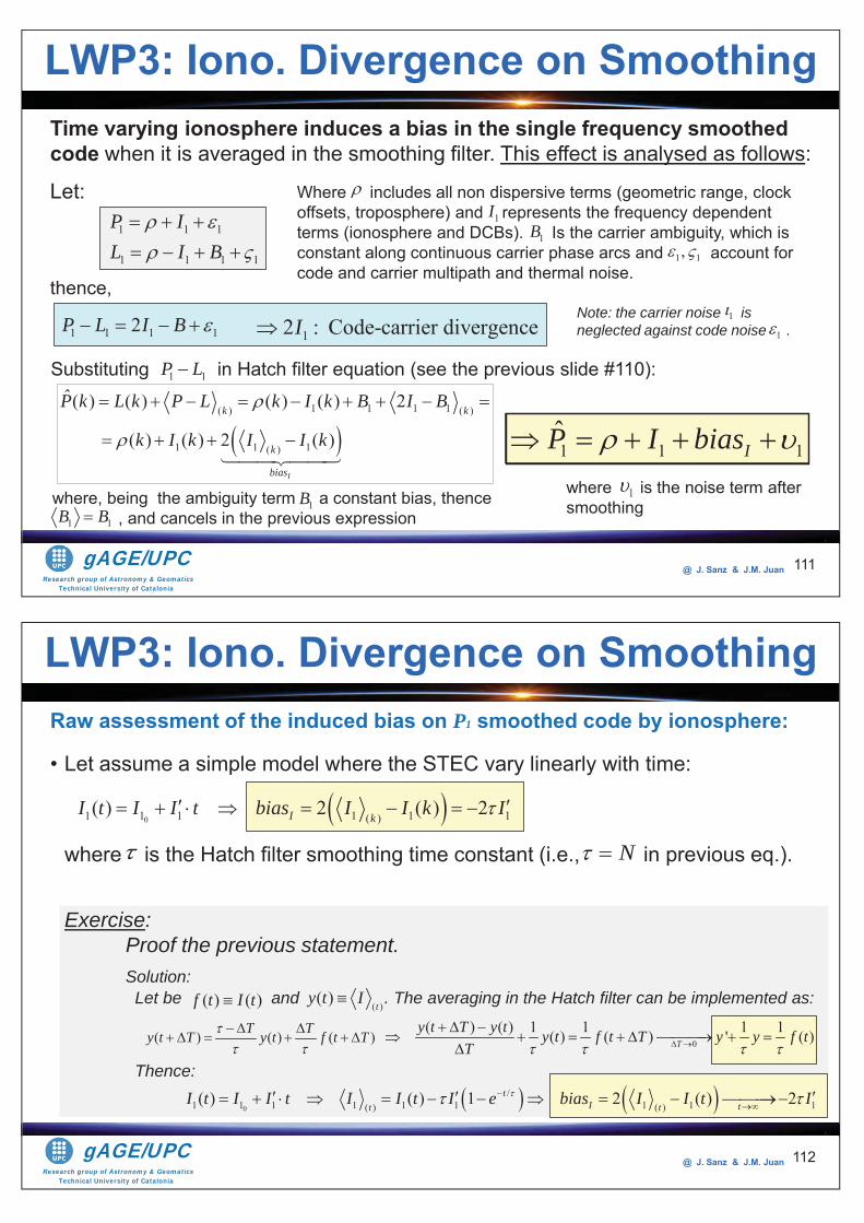
Research group of Astronomy & GeomaticsTechnical University of Catalonia
gAGE/UPC @ J. Sanz & J.M. Juan 111
Time varying ionosphere induces a bias in the single frequency smoothed code when it is averaged in the smoothing filter. This effect is analysed as follows:
Let:
LWP3: Iono. Divergence on Smoothing
1 1 1
1 1 1 1
P IL I B
thence,
1 1 1 12P L I B 12 : Code-carrier divergenceI
Substituting in Hatch filter equation (see the previous slide #110):1 1P L
1 1 1ˆ
IP I bias
where, being the ambiguity term a constant bias, thence , and cancels in the previous expression
1B1 1B B
1 1 1 1( ) ( )
1 1 1( )
ˆ ( ) ( ) ( ) ( ) 2
( ) ( ) 2 ( )
I
k k
k
bias
P k L k P L k I k B I B
k I k I I k
where is the noise term after smoothing
1
Note: the carrier noise is neglected against code noise .1
1
1I1B
1 1,
Where includes all non dispersive terms (geometric range, clock offsets, troposphere) and represents the frequency dependent terms (ionosphere and DCBs). Is the carrier ambiguity, which is constant along continuous carrier phase arcs and account for code and carrier multipath and thermal noise.
Research group of Astronomy & GeomaticsTechnical University of Catalonia
gAGE/UPC @ J. Sanz & J.M. Juan 112
Raw assessment of the induced bias on P1 smoothed code by ionosphere:
• Let assume a simple model where the STEC vary linearly with time:
where is the Hatch filter smoothing time constant (i.e., in previous eq.).
Exercise: Proof the previous statement.Solution: Let be and . The averaging in the Hatch filter can be implemented as:
Thence:
LWP3: Iono. Divergence on Smoothing
01 1 1 1 1 1( )( ) 2 ( ) 2I kI t I I t bias I I k I
N
( ) ( )f t I t ( )( )t
y t I
( ) ( ) ( )T Ty t T y t f t T 0( ) ( ) 1 1 1 1( ) ( ) ' ( )T
y t T y t y t f t T y y f tT
0
/1 1 1 1 1 1 1 1 1( ) ( )( ) ( ) 1 2 ( ) 2t
I tt tI t I I t I I t I e bias I I t I
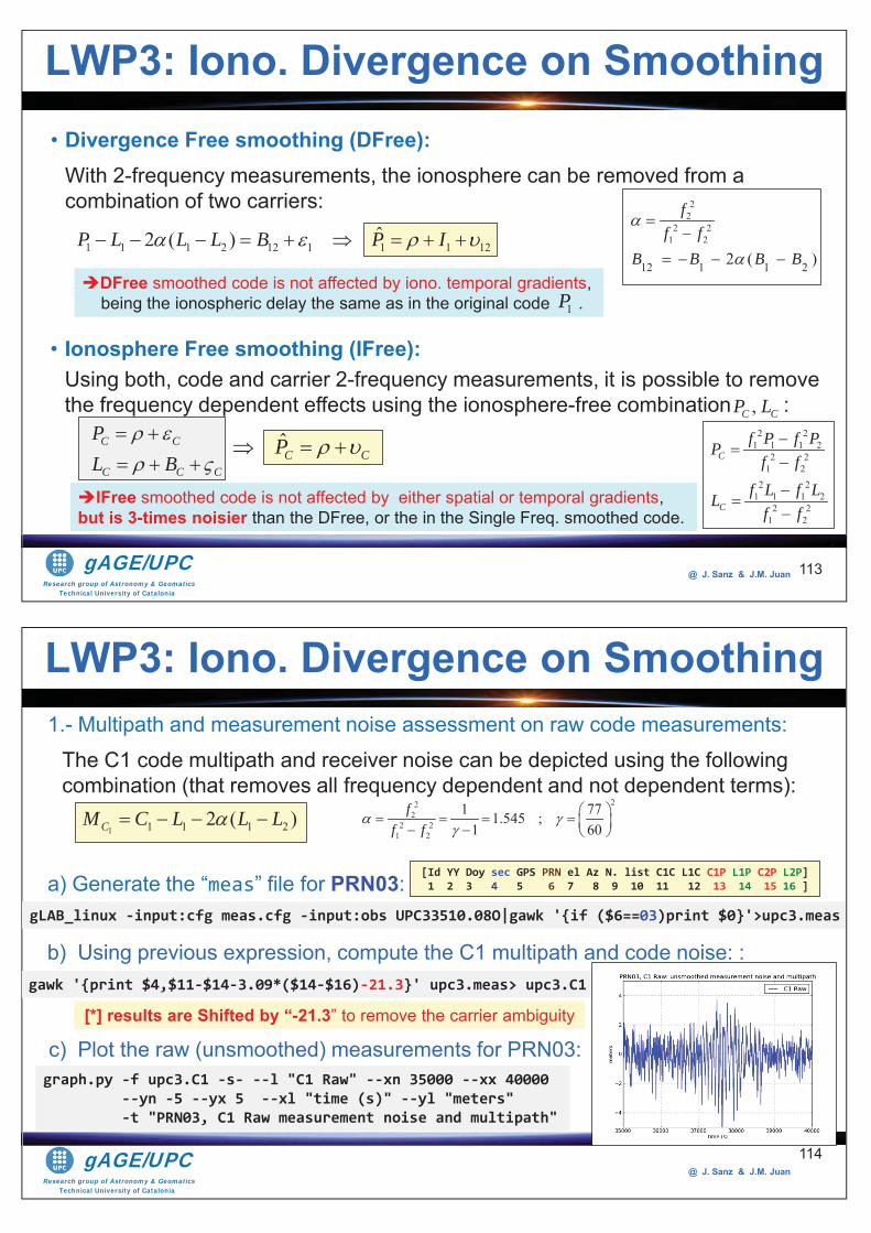
Research group of Astronomy & GeomaticsTechnical University of Catalonia
gAGE/UPC @ J. Sanz & J.M. Juan 113
• Divergence Free smoothing (DFree):With 2-frequency measurements, the ionosphere can be removed from a combination of two carriers:
LWP3: Iono. Divergence on Smoothing
1 1 1 2 12 1 1 1 12ˆ2 ( )P L L L B P I
22
2 21 2
ff f
12 1 1 22 ( )B B B B
• Ionosphere Free smoothing (IFree):Using both, code and carrier 2-frequency measurements, it is possible to remove the frequency dependent effects using the ionosphere-free combination :
C C
C C C
PL B
2 21 1 1 2
2 21 2
2 21 1 1 2
2 21 2
C
C
f P f PPf f
f L f LLf f
,C CP L
C CP
DFree smoothed code is not affected by iono. temporal gradients, being the ionospheric delay the same as in the original code .1P
IFree smoothed code is not affected by either spatial or temporal gradients,but is 3-times noisier than the DFree, or the in the Single Freq. smoothed code.
Research group of Astronomy & GeomaticsTechnical University of Catalonia
gAGE/UPC @ J. Sanz & J.M. Juan
114
LWP3: Iono. Divergence on Smoothing 1.- Multipath and measurement noise assessment on raw code measurements:
The C1 code multipath and receiver noise can be depicted using the following combination (that removes all frequency dependent and not dependent terms):
a) Generate the “meas” file for PRN03:
1 1 1 1 22 ( )CM C L L L
gLAB_linux -input:cfg meas.cfg -input:obs UPC33510.08O|gawk '{if ($6==03)print $0}'>upc3.meas
gawk '{print $4,$11-$14-3.09*($14-$16)-21.3}' upc3.meas> upc3.C1
c) Plot the raw (unsmoothed) measurements for PRN03:
222
2 21 2
1 771.545 ;1 60
ff f
graph.py -f upc3.C1 -s- --l "C1 Raw" --xn 35000 --xx 40000 --yn -5 --yx 5 --xl "time (s)" --yl "meters" -t "PRN03, C1 Raw measurement noise and multipath"
[*] results are Shifted by “-21.3” to remove the carrier ambiguity
[Id YY Doy sec GPS PRN el Az N. list C1C L1C C1P L1P C2P L2P] 1 2 3 4 5 6 7 8 9 10 11 12 13 14 15 16 ]
b) Using previous expression, compute the C1 multipath and code noise: :
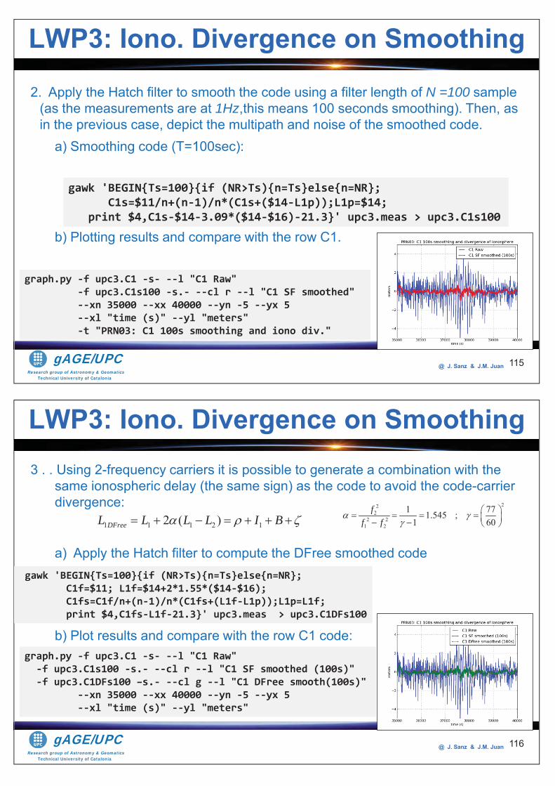
Research group of Astronomy & GeomaticsTechnical University of Catalonia
gAGE/UPC @ J. Sanz & J.M. Juan 115
LWP3: Iono. Divergence on Smoothing
2. Apply the Hatch filter to smooth the code using a filter length of N =100 sample (as the measurements are at 1Hz,this means 100 seconds smoothing). Then, as in the previous case, depict the multipath and noise of the smoothed code.
a) Smoothing code (T=100sec):
b) Plotting results and compare with the row C1.
gawk 'BEGIN{Ts=100}{if (NR>Ts){n=Ts}else{n=NR}; C1s=$11/n+(n-1)/n*(C1s+($14-L1p));L1p=$14; print $4,C1s-$14-3.09*($14-$16)-21.3}' upc3.meas > upc3.C1s100
graph.py -f upc3.C1 -s- --l "C1 Raw" -f upc3.C1s100 -s.- --cl r --l "C1 SF smoothed" --xn 35000 --xx 40000 --yn -5 --yx 5 --xl "time (s)" --yl "meters" -t "PRN03: C1 100s smoothing and iono div."
Research group of Astronomy & GeomaticsTechnical University of Catalonia
gAGE/UPC @ J. Sanz & J.M. Juan 116
LWP3: Iono. Divergence on Smoothing 3 . . Using 2-frequency carriers it is possible to generate a combination with the
same ionospheric delay (the same sign) as the code to avoid the code-carrier divergence:
a) Apply the Hatch filter to compute the DFree smoothed code
b) Plot results and compare with the row C1 code:
gawk 'BEGIN{Ts=100}{if (NR>Ts){n=Ts}else{n=NR}; C1f=$11; L1f=$14+2*1.55*($14-$16); C1fs=C1f/n+(n-1)/n*(C1fs+(L1f-L1p));L1p=L1f; print $4,C1fs-L1f-21.3}' upc3.meas > upc3.C1DFs100
222
2 21 2
1 771.545 ;1 60
ff f
graph.py -f upc3.C1 -s- --l "C1 Raw" -f upc3.C1s100 -s.- --cl r --l "C1 SF smoothed (100s)" -f upc3.C1DFs100 –s.- --cl g --l "C1 DFree smooth(100s)" --xn 35000 --xx 40000 --yn -5 --yx 5 --xl "time (s)" --yl "meters"
1 1 1 2 12 ( )DFreeL L L L I B
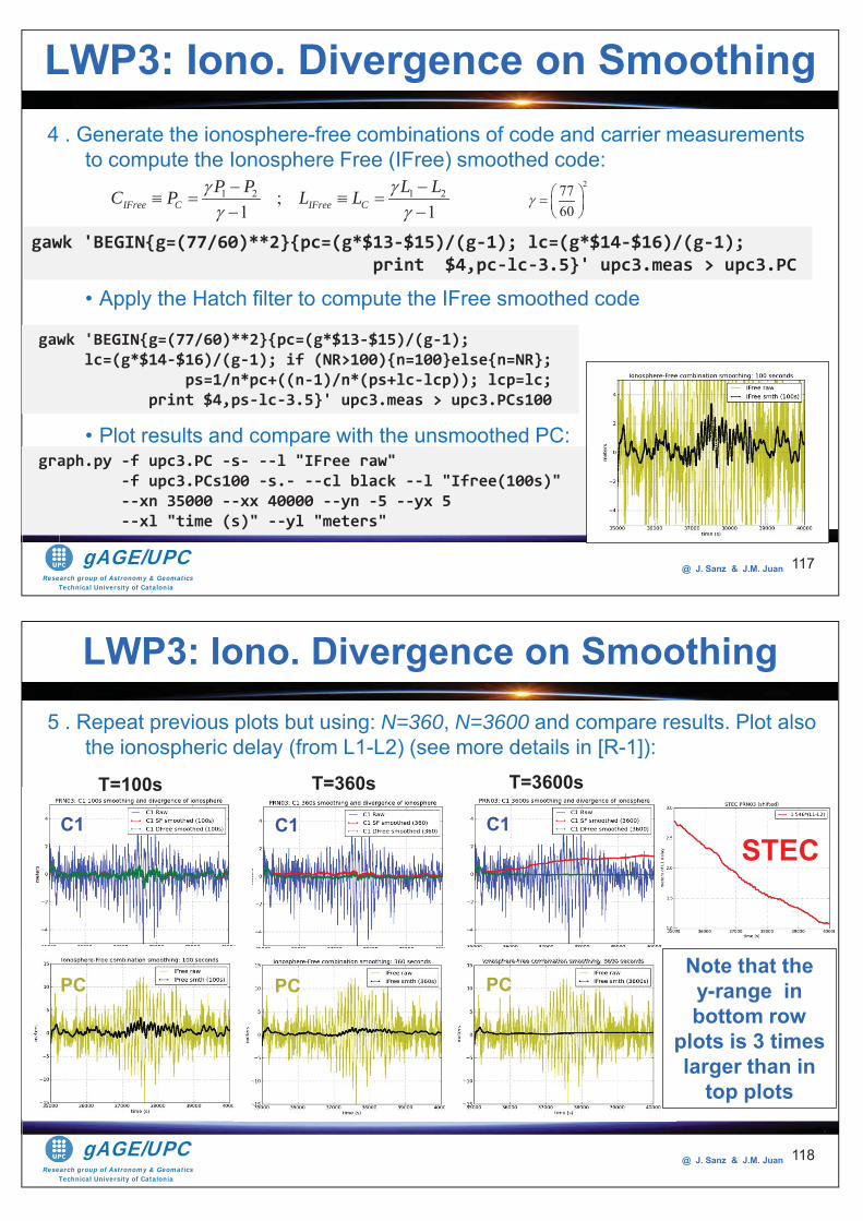
Research group of Astronomy & GeomaticsTechnical University of Catalonia
gAGE/UPC @ J. Sanz & J.M. Juan 117
LWP3: Iono. Divergence on Smoothing 4 . Generate the ionosphere-free combinations of code and carrier measurements
to compute the Ionosphere Free (IFree) smoothed code:
• Apply the Hatch filter to compute the IFree smoothed code
• Plot results and compare with the unsmoothed PC:
gawk 'BEGIN{g=(77/60)**2}{pc=(g*$13-$15)/(g-1); lc=(g*$14-$16)/(g-1); print $4,pc-lc-3.5}' upc3.meas > upc3.PC
27760
1 2 1 2;1 1IFree C IFree C
P P L LC P L L
gawk 'BEGIN{g=(77/60)**2}{pc=(g*$13-$15)/(g-1); lc=(g*$14-$16)/(g-1); if (NR>100){n=100}else{n=NR}; ps=1/n*pc+((n-1)/n*(ps+lc-lcp)); lcp=lc; print $4,ps-lc-3.5}' upc3.meas > upc3.PCs100
graph.py -f upc3.PC -s- --l "IFree raw" -f upc3.PCs100 -s.- --cl black --l "Ifree(100s)" --xn 35000 --xx 40000 --yn -5 --yx 5 --xl "time (s)" --yl "meters"
Research group of Astronomy & GeomaticsTechnical University of Catalonia
gAGE/UPC @ J. Sanz & J.M. Juan 118
LWP3: Iono. Divergence on Smoothing 5 . Repeat previous plots but using: N=360, N=3600 and compare results. Plot also
the ionospheric delay (from L1-L2) (see more details in [R-1]):
STEC
Note that the y-range in bottom row
plots is 3 times larger than in
top plots
T=100s T=360s T=3600s
C1
PC
C1
PC
C1
PC
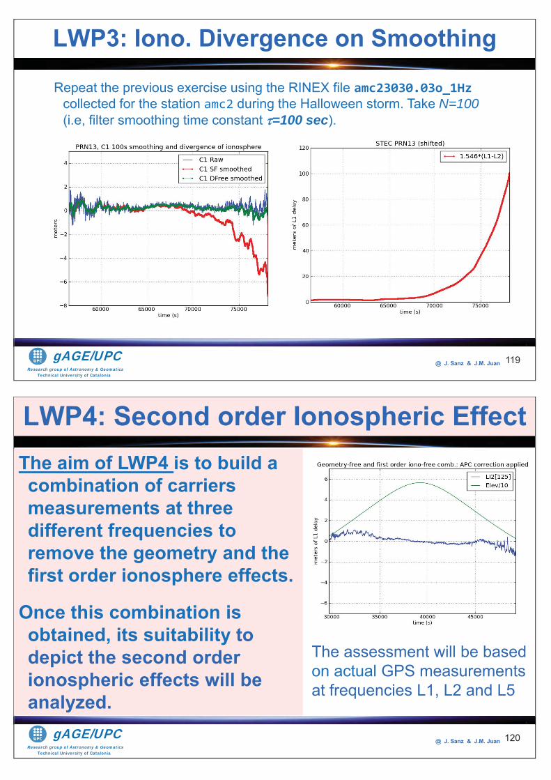
Research group of Astronomy & GeomaticsTechnical University of Catalonia
gAGE/UPC @ J. Sanz & J.M. Juan 119
Repeat the previous exercise using the RINEX file amc23030.03o_1Hz collected for the station amc2 during the Halloween storm. Take N=100(i.e, filter smoothing time constant =100 sec).
LWP3: Iono. Divergence on Smoothing
Research group of Astronomy & GeomaticsTechnical University of Catalonia
gAGE/UPC @ J. Sanz & J.M. Juan 120
The aim of LWP4 is to build a combination of carriers measurements at three different frequencies to remove the geometry and the first order ionosphere effects.
Once this combination is obtained, its suitability to depict the second order ionospheric effects will be analyzed.
LWP4: Second order Ionospheric Effect
The assessment will be based on actual GPS measurements at frequencies L1, L2 and L5
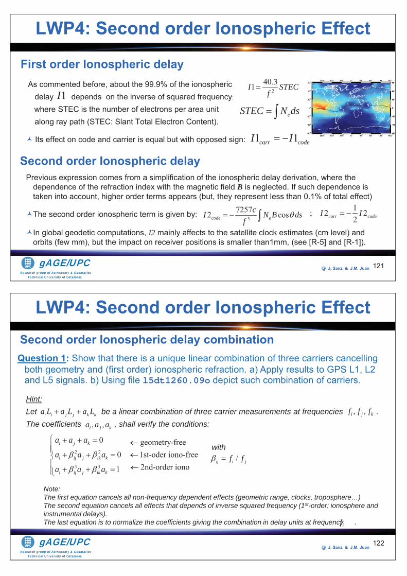
Research group of Astronomy & GeomaticsTechnical University of Catalonia
gAGE/UPC @ J. Sanz & J.M. Juan
As commented before, about the 99.9% of the ionospheric delay depends on the inverse of squared frequency:
where STEC is the number of electrons per area unit along ray path (STEC: Slant Total Electron Content).
Its effect on code and carrier is equal but with opposed sign:
121
240.31I STECf
eSTEC N ds1I
First order Ionospheric delay
1 1carr codeI I
Second order Ionospheric delayPrevious expression comes from a simplification of the ionospheric delay derivation, where the
dependence of the refraction index with the magnetic field B is neglected. If such dependence is taken into account, higher order terms appears (but, they represent less than 0.1% of total effect)
The second order ionospheric term is given by:
In global geodetic computations, I2 mainly affects to the satellite clock estimates (cm level) and orbits (few mm), but the impact on receiver positions is smaller than1mm, (see [R-5] and [R-1]).
372572 coscode e
cI N B dsf
1; 2 22carr codeI I
LWP4: Second order Ionospheric Effect
Research group of Astronomy & GeomaticsTechnical University of Catalonia
gAGE/UPC @ J. Sanz & J.M. Juan
122
, ,i j kf f f
/ij i jf fwith
Question 1: Show that there is a unique linear combination of three carriers cancelling both geometry and (first order) ionospheric refraction. a) Apply results to GPS L1, L2 and L5 signals. b) Using file l5dt1260.09o depict such combination of carriers.
i i j j k ka L a L a L, ,i j ka a a
2 2
3 3
0 geometry-free0 1st-oder iono-free
2nd-order iono1
i j k
i ij j ik k
i ij j ik k
a a a
a a a
a a a
Note: The first equation cancels all non-frequency dependent effects (geometric range, clocks, troposphere…)The second equation cancels all effects that depends of inverse squared frequency (1st-order: ionosphere and instrumental delays).The last equation is to normalize the coefficients giving the combination in delay units at frequency .if
Second order Ionospheric delay combination
Hint:Let be a linear combination of three carrier measurements at frequencies .The coefficients , shall verify the conditions:
LWP4: Second order Ionospheric Effect
estiooth g
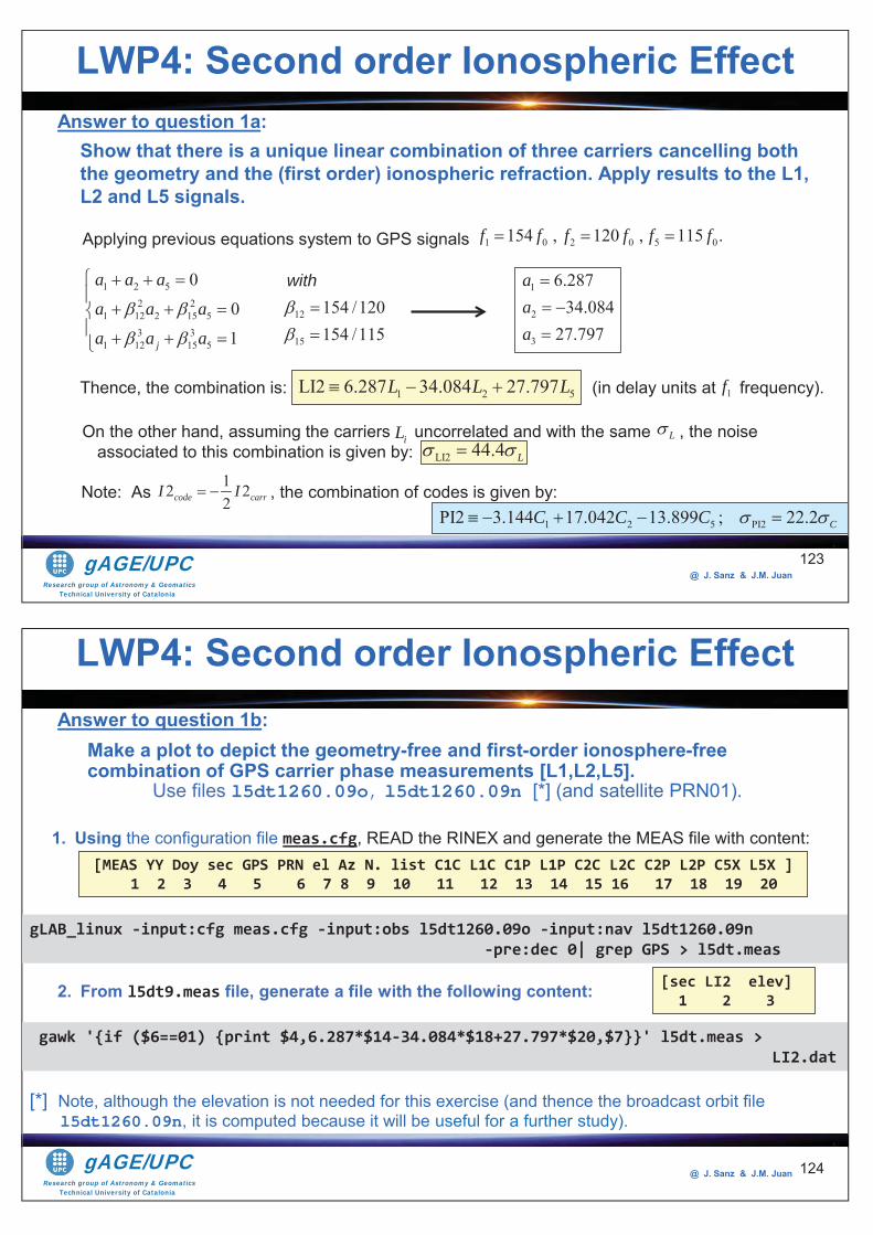
Research group of Astronomy & GeomaticsTechnical University of Catalonia
gAGE/UPC @ J. Sanz & J.M. Juan
123
12
15
154 /120154 /115
with1 2 52 2
1 12 2 15 53 3
1 12 15 5
001j
a a aa a aa a a
Thence, the combination is: (in delay units at frequency).
Answer to question 1a:Show that there is a unique linear combination of three carriers cancelling both the geometry and the (first order) ionospheric refraction. Apply results to the L1, L2 and L5 signals.
1 0 2 0 5 0154 , 120 , 115 .f f f f f fApplying previous equations system to GPS signals
1
2
3
6.28734.084
27.797
aaa
1 2 5LI2 6.287 34.084 27.797L L L
LI2 44.4 L
1f
On the other hand, assuming the carriers uncorrelated and with the same , the noise associated to this combination is given by:
iL L
Note: As , the combination of codes is given by:
1 2 5 PI2PI2 3.144 17.042 13.899 ; 22.2 CC C C
12 22code carrI I
LWP4: Second order Ionospheric Effect
theL2
Research group of Astronomy & GeomaticsTechnical University of Catalonia
gAGE/UPC @ J. Sanz & J.M. Juan 124
gLAB_linux -input:cfg meas.cfg -input:obs l5dt1260.09o -input:nav l5dt1260.09n -pre:dec 0| grep GPS > l5dt.meas
[MEAS YY Doy sec GPS PRN el Az N. list C1C L1C C1P L1P C2C L2C C2P L2P C5X L5X ] 1 2 3 4 5 6 7 8 9 10 11 12 13 14 15 16 17 18 19 20
1. Using the configuration file meas.cfg, READ the RINEX and generate the MEAS file with content:
gawk '{if ($6==01) {print $4,6.287*$14-34.084*$18+27.797*$20,$7}}' l5dt.meas > LI2.dat
2. From l5dt9.meas file, generate a file with the following content: [sec LI2 elev] 1 2 3
Answer to question 1b:Make a plot to depict the geometry-free and first-order ionosphere-free combination of GPS carrier phase measurements [L1,L2,L5].
Use files l5dt1260.09o, l5dt1260.09n [*] (and satellite PRN01).
[*] Note, although the elevation is not needed for this exercise (and thence the broadcast orbit file l5dt1260.09n, it is computed because it will be useful for a further study).
LWP4: Second order Ionospheric Effect
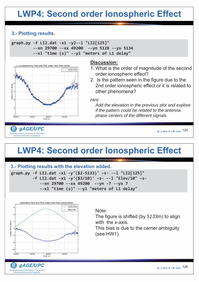
Research group of Astronomy & GeomaticsTechnical University of Catalonia
gAGE/UPC @ J. Sanz & J.M. Juan 125
graph.py -f LI2.dat -x1 -y2--l "LI2[125]" --xn 29700 --xx 49200 --yn 5128 --yx 5134 --xl "time (s)" --yl "meters of L1 delay"
3.- Plotting results:
Discussion:1. What is the order of magnitude of the second
order ionospheric effect?2. Is the pattern seen in the figure due to the
2nd order ionospheric effect or it is related to other phenomena?
Hint:Add the elevation in the previous plot and explore if the pattern could be related to the antenna phase centers of the different signals.
LWP4: Second order Ionospheric Effect
Research group of Astronomy & GeomaticsTechnical University of Catalonia
gAGE/UPC @ J. Sanz & J.M. Juan 126
graph.py -f LI2.dat -x1 -y'($2-5133)' –s- --l "LI2[125]" -f LI2.dat -x1 -y'($3/10)' –s- --l "Elev/10" –s- --xn 29700 --xx 49200 --yn -7 --yx 7 --xl "time (s)" --yl "meters of L1 delay"
3.- Plotting results with the elevation added:
Note: The figure is shifted (by 5133m) to align with the x-axis.This bias is due to the carrier ambiguity(see HW1).
LWP4: Second order Ionospheric Effect
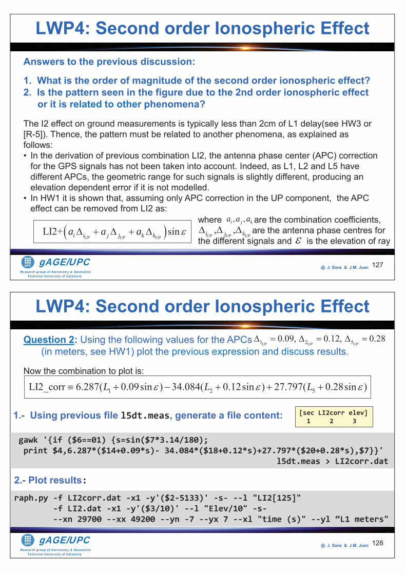
Research group of Astronomy & GeomaticsTechnical University of Catalonia
gAGE/UPC @ J. Sanz & J.M. Juan 127
Answers to the previous discussion:
1. What is the order of magnitude of the second order ionospheric effect?2. Is the pattern seen in the figure due to the 2nd order ionospheric effect
or it is related to other phenomena?
The I2 effect on ground measurements is typically less than 2cm of L1 delay(see HW3 or [R-5]). Thence, the pattern must be related to another phenomena, as explained as follows:• In the derivation of previous combination LI2, the antenna phase center (APC) correction
for the GPS signals has not been taken into account. Indeed, as L1, L2 and L5 have different APCs, the geometric range for such signals is slightly different, producing an elevation dependent error if it is not modelled.
• In HW1 it is shown that, assuming only APC correction in the UP component, the APC effect can be removed from LI2 as:
LI2+ sinUP UP UPi i j j k ka a a
where are the combination coefficients, are the antenna phase centres for the different signals and is the elevation of ray
, ,i j ka a a, ,
UP UP UPi j k
LWP4: Second order Ionospheric Effect
Research group of Astronomy & GeomaticsTechnical University of Catalonia
gAGE/UPC @ J. Sanz & J.M. Juan 128
Question 2: Using the following values for the APCs (in meters, see HW1) plot the previous expression and discuss results.
Now the combination to plot is:
1 2 50.09, 0.12, 0.28UP UP UP
1 2 5LI2_corr 6.287( 0.09sin ) 34.084( 0.12sin ) 27.797( 0.28sin )L L L
gawk '{if ($6==01) {s=sin($7*3.14/180); print $4,6.287*($14+0.09*s)- 34.084*($18+0.12*s)+27.797*($20+0.28*s),$7}}' l5dt.meas > LI2corr.dat
1.- Using previous file l5dt.meas, generate a file content: [sec LI2corr elev] 1 2 3
raph.py -f LI2corr.dat -x1 -y'($2-5133)' -s- --l "LI2[125]" -f LI2.dat -x1 -y'($3/10)' --l "Elev/10" -s- --xn 29700 --xx 49200 --yn -7 --yx 7 --xl "time (s)" --yl “L1 meters"
2.- Plot results:
LWP4: Second order Ionospheric Effect
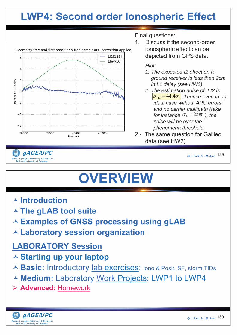
Research group of Astronomy & GeomaticsTechnical University of Catalonia
gAGE/UPC @ J. Sanz & J.M. Juan 129
Final questions:1. Discuss if the second-order
ionospheric effect can be depicted from GPS data.Hint:1. The expected I2 effect on a
ground receiver is less than 2cm in L1 delay (see HW3)
2. The estimation noise of LI2 is . .Thence even in an ideal case without APC errors and no carrier multipath (take for instance ), the noise will be over the phenomena threshold. 2.- The same question for Galileo
data (see HW2).
LI2 44.4 L
2L mm
LWP4: Second order Ionospheric Effect
Research group of Astronomy & GeomaticsTechnical University of Catalonia
gAGE/UPC @ J. Sanz & J.M. Juan
IntroductionThe gLAB tool suiteExamples of GNSS processing using gLABLaboratory session organization
LABORATORY SessionStarting up your laptopBasic: Introductory lab exercises: Iono & Posit, SF, storm,TIDs
Medium: Laboratory Work Projects: LWP1 to LWP4Advanced: Homework
OVERVIEW
130
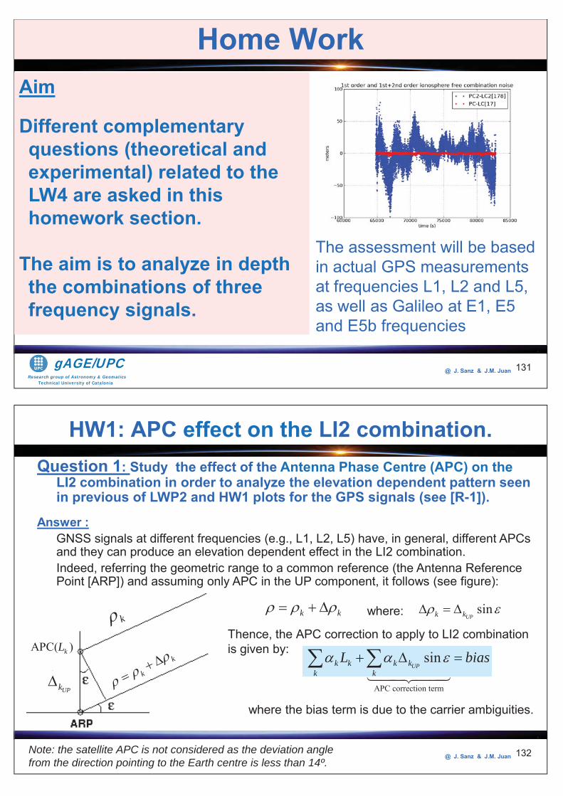
Research group of Astronomy & GeomaticsTechnical University of Catalonia
gAGE/UPC @ J. Sanz & J.M. Juan 131
Aim
Different complementary questions (theoretical and experimental) related to the LW4 are asked in this homework section.
The aim is to analyze in depth the combinations of three frequency signals.
Home Work
The assessment will be based in actual GPS measurements at frequencies L1, L2 and L5, as well as Galileo at E1, E5 and E5b frequencies
Research group of Astronomy & GeomaticsTechnical University of Catalonia
gAGE/UPC @ J. Sanz & J.M. Juan 132
Question 1: Study the effect of the Antenna Phase Centre (APC) on the LI2 combination in order to analyze the elevation dependent pattern seen in previous of LWP2 and HW1 plots for the GPS signals (see [R-1]).
Answer :GNSS signals at different frequencies (e.g., L1, L2, L5) have, in general, different APCs and they can produce an elevation dependent effect in the LI2 combination. Indeed, referring the geometric range to a common reference (the Antenna Reference Point [ARP]) and assuming only APC in the UP component, it follows (see figure):
k k sinUPk kk
where:
k
k
UPk
APC( )kLThence, the APC correction to apply to LI2 combination is given by:
APC correction term
sinUPk k k k
k kL bias
where the bias term is due to the carrier ambiguities.
Note: the satellite APC is not considered as the deviation angle from the direction pointing to the Earth centre is less than 14º.
HW1: APC effect on the LI2 combination.
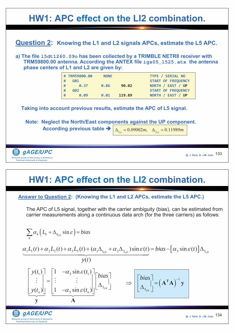
Research group of Astronomy & GeomaticsTechnical University of Catalonia
gAGE/UPC @ J. Sanz & J.M. Juan 133
Question 2: Knowing the L1 and L2 signals APCs, estimate the L5 APC.
a) The file l5dt1260.09o has been collected by a TRIMBLE NETR8 receiver with TRM59800.00 antenna. According the ANTEX file igs05_1525.atx the antenna phase centers of L1 and L2 are given by:
Taking into account previous results, estimate the APC of L5 signal.
Note: Neglect the North/East components against the UP component. According previous table
# TRM59800.00 NONE TYPE / SERIAL NO # G01 START OF FREQUENCY # 0.37 0.86 90.02 NORTH / EAST / UP # G02 START OF FREQUENCY # 0.09 0.01 119.89 NORTH / EAST / UP
HW1: APC effect on the LI2 combination.
1 20.09002 , 0.11989UP UP
m m
Research group of Astronomy & GeomaticsTechnical University of Catalonia
gAGE/UPC @ J. Sanz & J.M. Juan 134
Answer to Question 2: (Knowing the L1 and L2 APCs, estimate the L5 APC.)
The APC of L5 signal, together with the carrier ambiguity (bias), can be estimated from carrier measurements along a continuous data arch (for the three carriers) as follows:
1 1 2 2 5 5 1 1 2 2 5 5( ) ( ) ( ) ( )sin ( ) sin ( )
( )UP UP UP
L t L t L t t bias t
y t
1 5 1
55
( ) 1 sin ( )
( ) 1 sin ( ) UPn n
y t tbias
y t t
y A
1
5UP
bias TA A y
sinUPk k k
kL bias
HW1: APC effect on the LI2 combination.
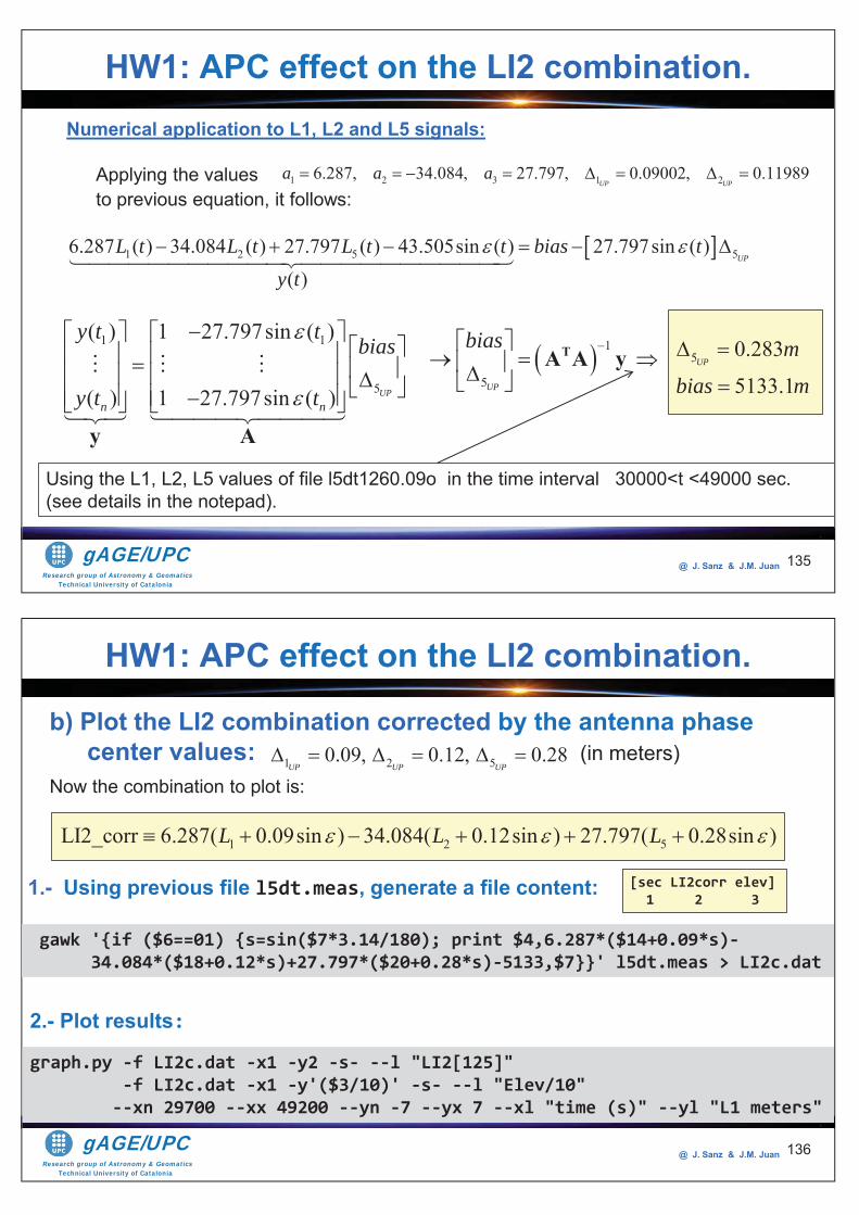
Research group of Astronomy & GeomaticsTechnical University of Catalonia
gAGE/UPC @ J. Sanz & J.M. Juan 135
Numerical application to L1, L2 and L5 signals:
Applying the valuesto previous equation, it follows:
1 2 5 56.287 ( ) 34.084 ( ) 27.797 ( ) 43.505sin ( ) 27.797sin ( )( )
UPL t L t L t t bias t
y t
1 1
5
( ) 1 27.797sin ( )
( ) 1 27.797sin ( ) UPn n
y t tbias
y t t
y A
1
5UP
bias TA A y 5 0.2835133.1
UPm
bias m
Using the L1, L2, L5 values of file l5dt1260.09o in the time interval 30000<t <49000 sec.(see details in the notepad).
1 2 3 1 26.287, 34.084, 27.797, 0.09002, 0.11989UP UP
a a a
HW1: APC effect on the LI2 combination.
Research group of Astronomy & GeomaticsTechnical University of Catalonia
gAGE/UPC @ J. Sanz & J.M. Juan 136
b) Plot the LI2 combination corrected by the antenna phase center values: (in meters)
Now the combination to plot is:1 2 50.09, 0.12, 0.28
UP UP UP
1 2 5LI2_corr 6.287( 0.09sin ) 34.084( 0.12sin ) 27.797( 0.28sin )L L L
gawk '{if ($6==01) {s=sin($7*3.14/180); print $4,6.287*($14+0.09*s)- 34.084*($18+0.12*s)+27.797*($20+0.28*s)-5133,$7}}' l5dt.meas > LI2c.dat
1.- Using previous file l5dt.meas, generate a file content: [sec LI2corr elev] 1 2 3
graph.py -f LI2c.dat -x1 -y2 -s- --l "LI2[125]" -f LI2c.dat -x1 -y'($3/10)' -s- --l "Elev/10" --xn 29700 --xx 49200 --yn -7 --yx 7 --xl "time (s)" --yl "L1 meters"
2.- Plot results:
HW1: APC effect on the LI2 combination.
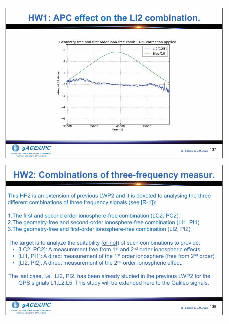
Research group of Astronomy & GeomaticsTechnical University of Catalonia
gAGE/UPC @ J. Sanz & J.M. Juan 137
HW1: APC effect on the LI2 combination.
Research group of Astronomy & GeomaticsTechnical University of Catalonia
gAGE/UPC @ J. Sanz & J.M. Juan 138
This HP2 is an extension of previous LWP2 and it is devoted to analysing the three different combinations of three frequency signals (see [R-1]):
1.The first and second order ionosphere-free combination (LC2, PC2).2.The geometry-free and second-order ionosphere-free combination (LI1, PI1).3.The geometry-free and first-order ionosphere-free combination (LI2, PI2).
HW2: Combinations of three-frequency measur.
The target is to analyze the suitability (or not) of such combinations to provide:• [LC2, PC2]: A measurement free from 1st and 2nd order ionospheric effects.• [LI1, PI1]: A direct measurement of the 1st order ionosphere (free from 2nd order). • [LI2, PI2]: A direct measurement of the 2nd order ionospheric effect.
The last case, i.e. LI2, PI2, has been already studied in the previous LWP2 for the GPS signals L1,L2,L5. This study will be extended here to the Galileo signals.
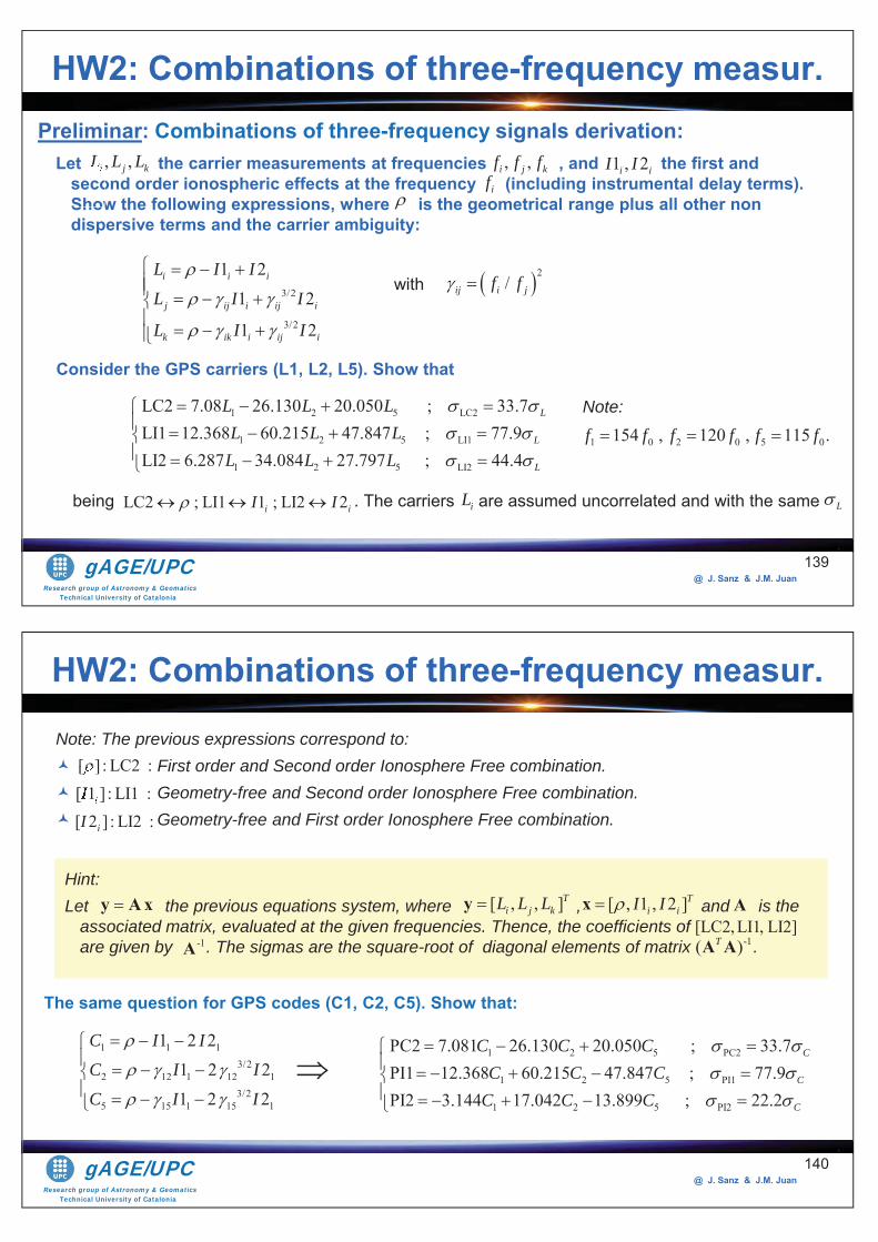
Research group of Astronomy & GeomaticsTechnical University of Catalonia
gAGE/UPC @ J. Sanz & J.M. Juan
139
Let the carrier measurements at frequencies , and the first and second order ionospheric effects at the frequency (including instrumental delay terms). Show the following expressions, where is the geometrical range plus all other non dispersive terms and the carrier ambiguity:
, ,i j kL L L , ,i j kf f f 1 , 2i iI Iif
3/2
3/2
1 21 2
1 2
i i i
j ij i ij i
k ik i ij i
L I IL I I
L I I
2/ij i jf fwith
Consider the GPS carriers (L1, L2, L5). Show that
1 2 5 LC2
1 2 5 LI1
1 2 5 LI2
LC2 7.08 26.130 20.050 ; 33.7LI1 12.368 60.215 47.847 ; 77.9LI2 6.287 34.084 27.797 ; 44.4
L
L
L
L L LL L L
L L L
being . The carriers are assumed uncorrelated and with the same iLLC2 ; LI1 1 ; LI2 2i iI I L
Note:
1 0 2 0 5 0154 , 120 , 115 .f f f f f f
HW2: Combinations of three-frequency measur.Preliminar: Combinations of three-frequency signals derivation:
et secoShow
Research group of Astronomy & GeomaticsTechnical University of Catalonia
gAGE/UPC @ J. Sanz & J.M. Juan
140
Note: The previous expressions correspond to: First order and Second order Ionosphere Free combination. Geometry-free and Second order Ionosphere Free combination. Geometry-free and First order Ionosphere Free combination.
Hint:Let the previous equations system, where , and is the
associated matrix, evaluated at the given frequencies. Thence, the coefficients of are given by . The sigmas are the square-root of diagonal elements of matrix .
[LC2,LI1, LI2]
[ ] : LC2 :[ 1 ] : LI1 :iI[ 2 ] : LI2 :iI
y Ax [ , , ]Ti j kL L Ly [ , 1 , 2 ]T
i iI Ix A
-1A -1( )TA A
1 2 5 PC2
1 2 5 PI1
1 2 5 PI2
PC2 7.081 26.130 20.050 ; 33.7PI1 12.368 60.215 47.847 ; 77.9PI2 3.144 17.042 13.899 ; 22.2
C
C
C
C C CC C C
C C C
The same question for GPS codes (C1, C2, C5). Show that:
1 1 13/2
2 12 1 12 13/2
5 15 1 15 1
1 2 21 2 21 2 2
C I IC I IC I I
HW2: Combinations of three-frequency measur.
[ ] : [ 1 ] i[
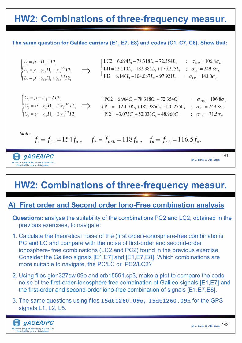
Research group of Astronomy & GeomaticsTechnical University of Catalonia
gAGE/UPC @ J. Sanz & J.M. Juan
141
1 7 8 PC2
1 7 8 PI1
1 7 8 PI2
PC2 6.964 78.318 72.354 ; 106.8PI1 12.110 182.385 170.275 ; 249.8PI2 3.073 52.033 48.960 ; 71.5
C
C
C
C C CC C C
C C C
The same question for Galileo carriers (E1, E7, E8) and codes (C1, C7, C8). Show that:
1 1 13/2
7 17 1 17 13/2
8 18 1 18 1
1 2 21 2 21 2 2
C I IC I IC I I
1 2 5 LC2
1 2 5 LI1
1 2 5 LI2
LC2 6.694 78.318 72.354 ; 106.8LI1 12.110 182.385 170.275 ; 249.8LI2 6.146 104.067 97.921 ; 143.0
L
L
L
L L LL L L
L L L
1 1 13/2
7 17 1 17 13/2
8 18 1 18 1
1 21 21 2
L I IL I IL I I
Note:
1 1 0 7 5 0 8 5 0154 , 118 , 116.5 .E E b Ef f f f f f f f f
HW2: Combinations of three-frequency measur.
Research group of Astronomy & GeomaticsTechnical University of Catalonia
gAGE/UPC @ J. Sanz & J.M. Juan 142
Questions: analyse the suitability of the combinations PC2 and LC2, obtained in the previous exercises, to navigate:
1. Calculate the theoretical noise of the (first order)-ionosphere-free combinations PC and LC and compare with the noise of first-order and second-order ionosphere- free combinations (LC2 and PC2) found in the previous exercise. Consider the Galileo signals [E1,E7] and [E1,E7,E8]. Which combinations are more suitable to navigate, the PC/LC or PC2/LC2?
2. Using files gien327sw.09o and orb15591.sp3, make a plot to compare the code noise of the first-order-ionosphere free combination of Galileo signals [E1,E7] and the first-order and second-order iono-free combination of signals [E1,E7,E8].
3. The same questions using files l5dt1260.09o, l5dt1260.09n for the GPS signals L1, L2, L5.
HW2: Combinations of three-frequency measur.
A) First order and Second order Iono-Free combination analysis
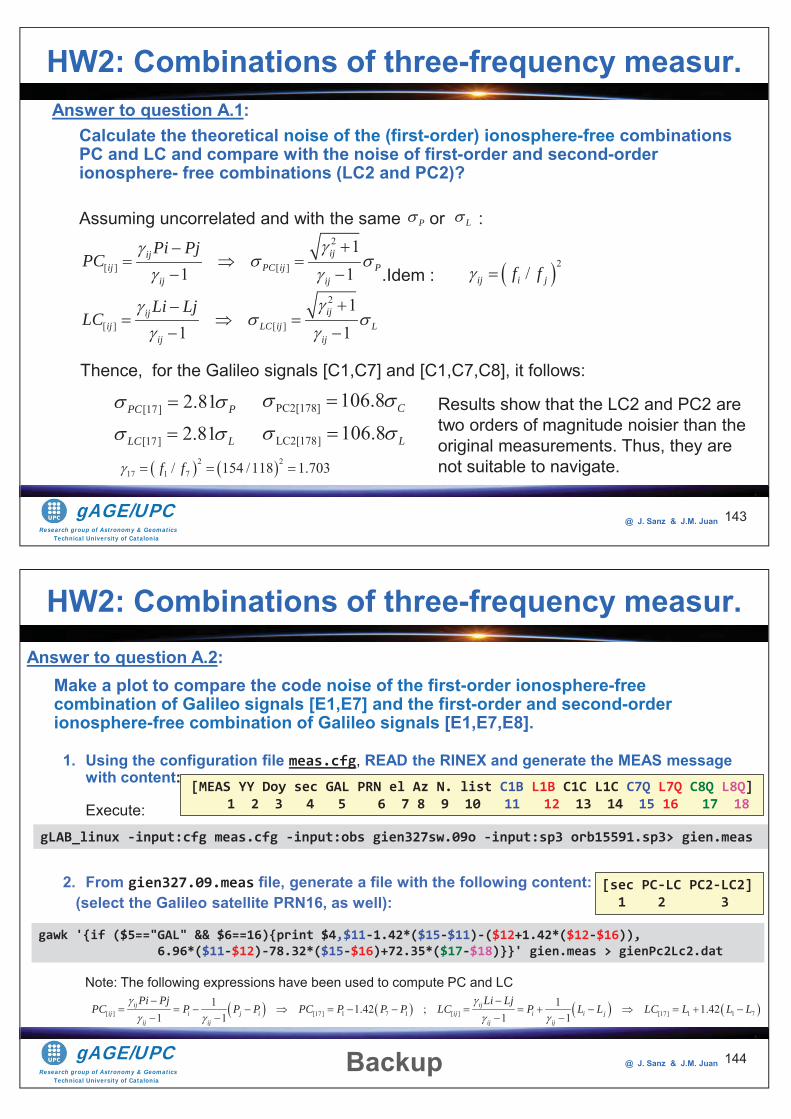
Research group of Astronomy & GeomaticsTechnical University of Catalonia
gAGE/UPC @ J. Sanz & J.M. Juan 143
Answer to question A.1:Calculate the theoretical noise of the (first-order) ionosphere-free combinations PC and LC and compare with the noise of first-order and second-order ionosphere- free combinations (LC2 and PC2)?
Assuming uncorrelated and with the same or :
P L
2
[ ] [ ]
11 1
ijijij PC ij P
ij ij
Pi PjPC 2
/ij i jf f.Idem :
Thence, for the Galileo signals [C1,C7] and [C1,C7,C8], it follows:
[17]
[17]
2.812.81
PC P
LC L
PC2[178]
LC2[178]
106.8106.8
C
L
Results show that the LC2 and PC2 are two orders of magnitude noisier than the original measurements. Thus, they are not suitable to navigate.
2
[ ] [ ]
11 1
ijijij LC ij L
ij ij
Li LjLC
2 217 1 7/ 154 /118 1.703f f
HW2: Combinations of three-frequency measur.
Research group of Astronomy & GeomaticsTechnical University of Catalonia
gAGE/UPC @ J. Sanz & J.M. Juan
Answer to question A.2:Make a plot to compare the code noise of the first-order ionosphere-free combination of Galileo signals [E1,E7] and the first-order and second-order ionosphere-free combination of Galileo signals [E1,E7,E8].
1. Using the configuration file meas.cfg, READ the RINEX and generate the MEAS message with content:
Execute:
2. From gien327.09.meas file, generate a file with the following content: (select the Galileo satellite PRN16, as well):
Note: The following expressions have been used to compute PC and LC
144
[MEAS YY Doy sec GAL PRN el Az N. list C1B L1B C1C L1C C7Q L7Q C8Q L8Q] 1 2 3 4 5 6 7 8 9 10 11 12 13 14 15 16 17 18
gawk '{if ($5=="GAL" && $6==16){print $4,$11-1.42*($15-$11)-($12+1.42*($12-$16)), 6.96*($11-$12)-78.32*($15-$16)+72.35*($17-$18)}}' gien.meas > gienPc2Lc2.dat
Backup
gLAB_linux -input:cfg meas.cfg -input:obs gien327sw.09o -input:sp3 orb15591.sp3> gien.meas
[sec PC-LC PC2-LC2] 1 2 3
[ ] [17] 1 7 1 [ ] [17] 1 1 71 11.42 ; 1.42
1 1 1 1ij ij
ij i j i ij i i jij ij ij ij
Pi Pj Li LjPC P P P PC P P P LC P L L LC L L L
HW2: Combinations of three-frequency measur.
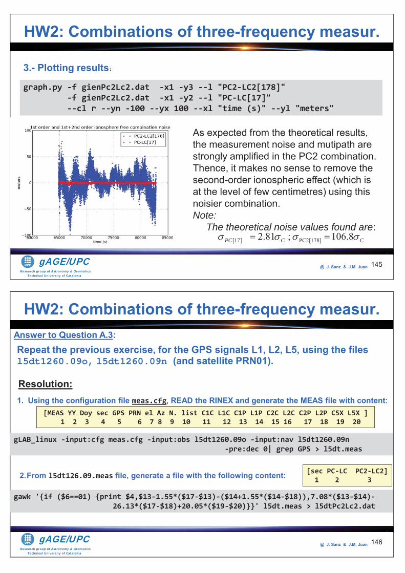
Research group of Astronomy & GeomaticsTechnical University of Catalonia
gAGE/UPC @ J. Sanz & J.M. Juan 145
graph.py -f gienPc2Lc2.dat -x1 -y3 --l "PC2-LC2[178]" -f gienPc2Lc2.dat -x1 -y2 --l "PC-LC[17]" --cl r --yn -100 --yx 100 --xl "time (s)" --yl "meters"
3.- Plotting results:
[17] PC2[178]2.81 ; 106.8PC C C
As expected from the theoretical results, the measurement noise and mutipath are strongly amplified in the PC2 combination. Thence, it makes no sense to remove the second-order ionospheric effect (which is at the level of few centimetres) using this noisier combination.Note: The theoretical noise values found are:
HW2: Combinations of three-frequency measur.
Research group of Astronomy & GeomaticsTechnical University of Catalonia
gAGE/UPC @ J. Sanz & J.M. Juan 146
Answer to Question A.3:Repeat the previous exercise, for the GPS signals L1, L2, L5, using the filesl5dt1260.09o, l5dt1260.09n (and satellite PRN01).
gLAB_linux -input:cfg meas.cfg -input:obs l5dt1260.09o -input:nav l5dt1260.09n -pre:dec 0| grep GPS > l5dt.meas
gawk '{if ($6==01) {print $4,$13-1.55*($17-$13)-($14+1.55*($14-$18)),7.08*($13-$14)- 26.13*($17-$18)+20.05*($19-$20)}}' l5dt.meas > l5dtPc2Lc2.dat
[MEAS YY Doy sec GPS PRN el Az N. list C1C L1C C1P L1P C2C L2C C2P L2P C5X L5X ] 1 2 3 4 5 6 7 8 9 10 11 12 13 14 15 16 17 18 19 20
1. Using the configuration file meas.cfg, READ the RINEX and generate the MEAS file with content:
2.From l5dt126.09.meas file, generate a file with the following content: [sec PC-LC PC2-LC2] 1 2 3
Resolution:
HW2: Combinations of three-frequency measur.
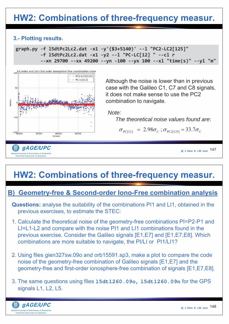
Research group of Astronomy & GeomaticsTechnical University of Catalonia
gAGE/UPC @ J. Sanz & J.M. Juan 147
graph.py -f l5dtPc2Lc2.dat -x1 -y'($3+5140)' --l "PC2-LC2[125]" -f l5dtPc2Lc2.dat -x1 -y2 --l "PC-LC[12] " --cl r --xn 29700 --xx 49200 --yn -100 --yx 100 --xl "time(s)" --yl "m"
3.- Plotting results:
[12] PC2[125]2.98 ; 33.7PC C C
Although the noise is lower than in previous case with the Galileo C1, C7 and C8 signals, it does not make sense to use the PC2 combination to navigate.
HW2: Combinations of three-frequency measur.
Note: The theoretical noise values found are:
Research group of Astronomy & GeomaticsTechnical University of Catalonia
gAGE/UPC @ J. Sanz & J.M. Juan 148
Questions: analyse the suitability of the combinations PI1 and LI1, obtained in the previous exercises, to estimate the STEC:
1. Calculate the theoretical noise of the geometry-free combinations PI=P2-P1 and LI=L1-L2 and compare with the noise PI1 and LI1 combinations found in the previous exercise. Consider the Galileo signals [E1,E7] and [E1,E7,E8]. Which combinations are more suitable to navigate, the PI/LI or PI1/LI1?
2. Using files gien327sw.09o and orb15591.sp3, make a plot to compare the code noise of the geometry-free combination of Galileo signals [E1,E7] and the geometry-free and first-order ionosphere-free combination of signals [E1,E7,E8].
3. The same questions using files l5dt1260.09o, l5dt1260.09n for the GPS signals L1, L2, L5.
HW2: Combinations of three-frequency measur.
B) Geometry-free & Second-order Iono-Free combination analysis
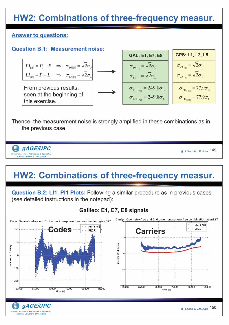
Research group of Astronomy & GeomaticsTechnical University of Catalonia
gAGE/UPC @ J. Sanz & J.M. Juan 149
Answer to questions:
Question B.1: Measurement noise:
Thence, the measurement noise is strongly amplified in these combinations as in the previous case.
[ ] [ ]
[ ] [ ]
2
2ij j i PI ij P
ij i j LI ij L
PI P P
LI P L
[178]
[178]
PI1
LI1
249.8
249.8C
L
[17 ]
[17 ]
2
2
PI C
LI L
[12]
[12]
2
2
PI C
LI L
[125]
[125]
PI1
LI1
77.9
77.9C
L
GAL: E1, E7, E8 GPS: L1, L2, L5
From previous results, seen at the beginning of this exercise.
HW2: Combinations of three-frequency measur.
Research group of Astronomy & GeomaticsTechnical University of Catalonia
gAGE/UPC @ J. Sanz & J.M. Juan 150
Question B.2: LI1, PI1 Plots: Following a similar procedure as in previous cases (see detailed instructions in the notepad):
Carriers
Galileo: E1, E7, E8 signals
HW2: Combinations of three-frequency measur.
Codes
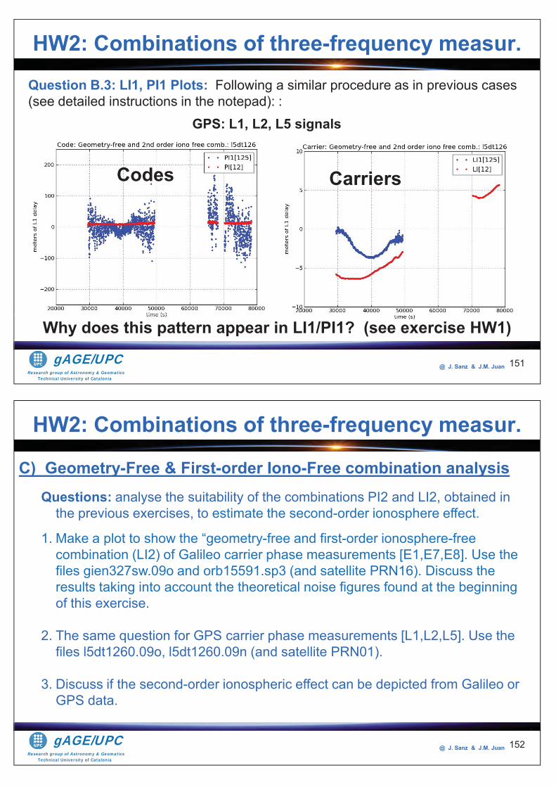
Research group of Astronomy & GeomaticsTechnical University of Catalonia
gAGE/UPC @ J. Sanz & J.M. Juan 151
Question B.3: LI1, PI1 Plots: Following a similar procedure as in previous cases (see detailed instructions in the notepad): :
GPS: L1, L2, L5 signals
Why does this pattern appear in LI1/PI1? (see exercise HW1)
HW2: Combinations of three-frequency measur.
CarriersCodes
Research group of Astronomy & GeomaticsTechnical University of Catalonia
gAGE/UPC @ J. Sanz & J.M. Juan 152
Questions: analyse the suitability of the combinations PI2 and LI2, obtained in the previous exercises, to estimate the second-order ionosphere effect.
1. Make a plot to show the “geometry-free and first-order ionosphere-free combination (LI2) of Galileo carrier phase measurements [E1,E7,E8]. Use the files gien327sw.09o and orb15591.sp3 (and satellite PRN16). Discuss the results taking into account the theoretical noise figures found at the beginning of this exercise.
2. The same question for GPS carrier phase measurements [L1,L2,L5]. Use the files l5dt1260.09o, l5dt1260.09n (and satellite PRN01).
3. Discuss if the second-order ionospheric effect can be depicted from Galileo or GPS data.
HW2: Combinations of three-frequency measur.
C) Geometry-Free & First-order Iono-Free combination analysis
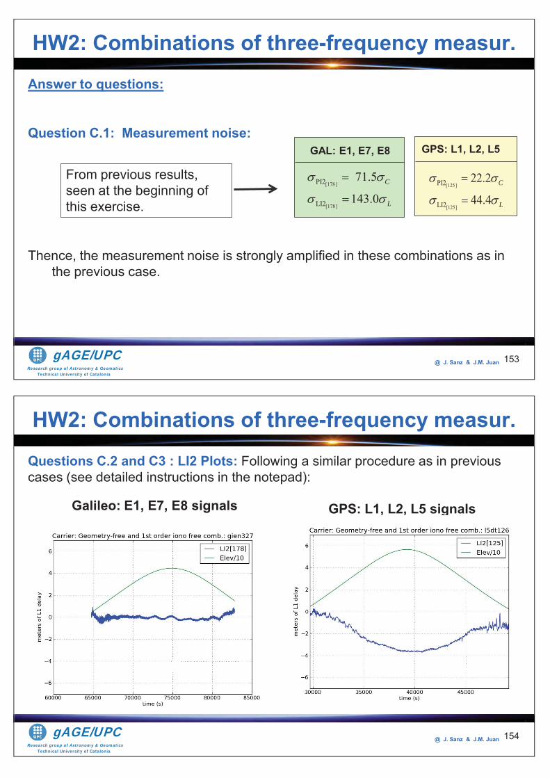
Research group of Astronomy & GeomaticsTechnical University of Catalonia
gAGE/UPC @ J. Sanz & J.M. Juan 153
Answer to questions:
Question C.1: Measurement noise:
Thence, the measurement noise is strongly amplified in these combinations as in the previous case.
[178]
[178]
PI2
LI2
71.5
143.0C
L
[125]
[125]
PI2
LI2
22.2
44.4C
L
GAL: E1, E7, E8 GPS: L1, L2, L5
From previous results, seen at the beginning of this exercise.
HW2: Combinations of three-frequency measur.
Research group of Astronomy & GeomaticsTechnical University of Catalonia
gAGE/UPC @ J. Sanz & J.M. Juan 154
Questions C.2 and C3 : LI2 Plots: Following a similar procedure as in previous cases (see detailed instructions in the notepad):
Galileo: E1, E7, E8 signals
HW2: Combinations of three-frequency measur.
Carriers
GPS: L1, L2, L5 signals
CarriersCCCCCCCCCCCCCCCCCarriiiiiiiiers
g
Carrieeeeeeeeeeeeeeers
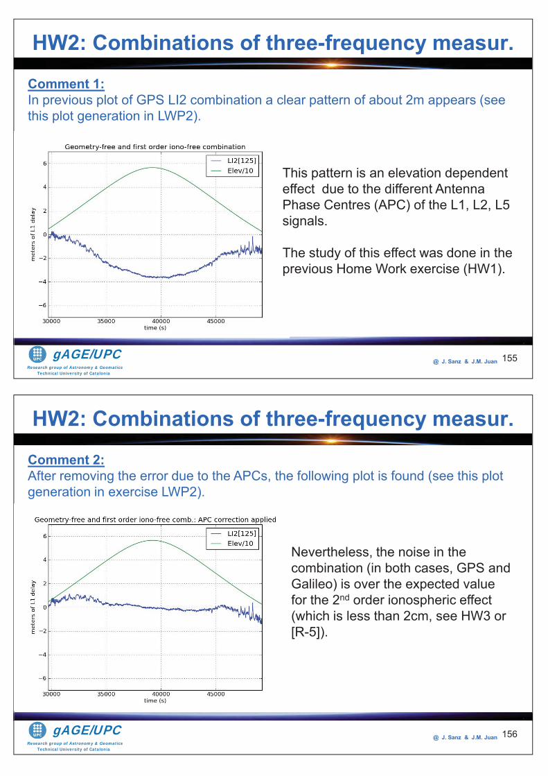
Research group of Astronomy & GeomaticsTechnical University of Catalonia
gAGE/UPC @ J. Sanz & J.M. Juan 155
Comment 1:In previous plot of GPS LI2 combination a clear pattern of about 2m appears (see this plot generation in LWP2).
HW2: Combinations of three-frequency measur.
This pattern is an elevation dependent effect due to the different Antenna Phase Centres (APC) of the L1, L2, L5 signals.
The study of this effect was done in the previous Home Work exercise (HW1).
Research group of Astronomy & GeomaticsTechnical University of Catalonia
gAGE/UPC @ J. Sanz & J.M. Juan 156
Comment 2:After removing the error due to the APCs, the following plot is found (see this plot generation in exercise LWP2).
HW2: Combinations of three-frequency measur.
Nevertheless, the noise in the combination (in both cases, GPS and Galileo) is over the expected value for the 2nd order ionospheric effect (which is less than 2cm, see HW3 or [R-5]).
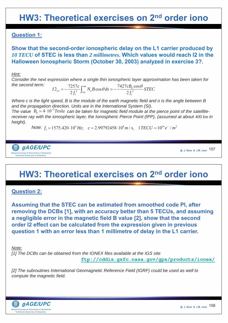
Research group of Astronomy & GeomaticsTechnical University of Catalonia
gAGE/UPC @ J. Sanz & J.M. Juan 157
Question 1:
Show that the second-order ionospheric delay on the L1 carrier produced by 10 TECU of STEC is less than 2 millimetres. Which values would reach I2 in the Halloween Ionospheric Storm (October 30, 2003) analyzed in exercise 3?.
Hint:Consider the next expression where a single thin ionospheric layer approximation has been taken for the second term:
Where c is the light speed, B is the module of the earth magnetic field and o is the angle between B and the propagation direction. Units are in the International System (SI).The value can be taken for magnetic field module at the pierce point of the satellite-receiver ray with the ionospheric layer, the Ionospheric Pierce Point (IPP), (assumed at about 400 km in height). Note:
HW3: Theoretical exercises on 2nd order iono
01 3 3
1 1
7427 cos72572 cos2 2
sat
L erec
cBcI N B ds STECf f
6 8 16 21 1575.420 10 ; 2.99792458 10 / , 1 10 /f Hz c m s TECU e m
50 4 10B Tesla
Research group of Astronomy & GeomaticsTechnical University of Catalonia
gAGE/UPC @ J. Sanz & J.M. Juan 158
Question 2:
Assuming that the STEC can be estimated from smoothed code PI, after removing the DCBs [1], with an accuracy better than 5 TECUs, and assuming a negligible error in the magnetic field B value [2], show that the second order I2 effect can be calculated from the expression given in previous question 1 with an error less than 1 millimetre of delay in the L1 carrier.
Note:[1] The DCBs can be obtained from the IONEX files available at the IGS site
ftp://cddis.gsfc.nasa.gov/gps/products/ionex/[2] The subroutines International Geomagnetic Reference Field (IGRF) could be used as well to compute the magnetic field.
HW3: Theoretical exercises on 2nd order iono
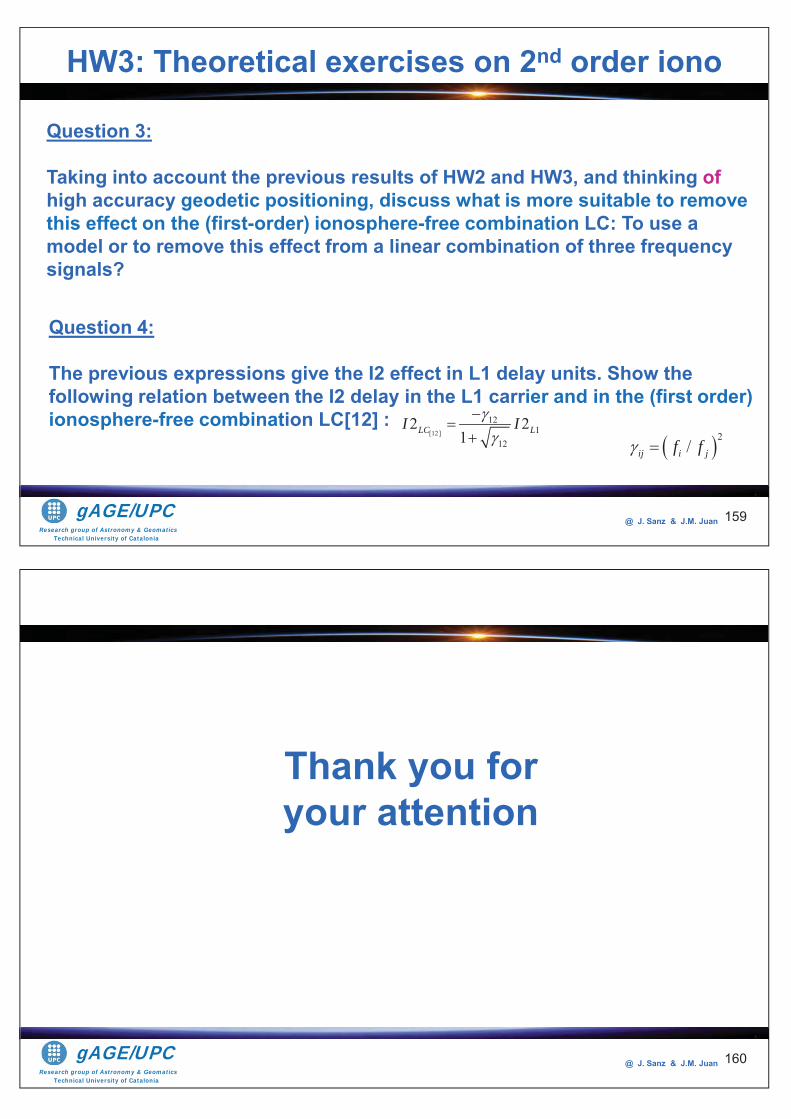
Research group of Astronomy & GeomaticsTechnical University of Catalonia
gAGE/UPC @ J. Sanz & J.M. Juan 159
Question 3:
Taking into account the previous results of HW2 and HW3, and thinking ofhigh accuracy geodetic positioning, discuss what is more suitable to remove this effect on the (first-order) ionosphere-free combination LC: To use a model or to remove this effect from a linear combination of three frequency signals?
HW3: Theoretical exercises on 2nd order iono
Question 4:
The previous expressions give the I2 effect in L1 delay units. Show the following relation between the I2 delay in the L1 carrier and in the (first order) ionosphere-free combination LC[12] :
[12]
121
12
2 21LC LI I
2/ij i jf f
Research group of Astronomy & GeomaticsTechnical University of Catalonia
gAGE/UPC @ J. Sanz & J.M. Juan 160
Thank you for your attention
Research group of Astronomy & GeomaticsTechnical University of Catalonia
gAGE/UPC @ J. Sanz & J.M. Juan 161
R-1: J. Sanz-Subirana, J.M. Jaun-Zoroza, M. Hernández-Pajares. GNSS Data processing. Volume-I and Volume-II. ESA Publications Division, 2012.R-2: J. Sanz-Subirana, J.M. Jaun-Zoroza, M. Hernández-Pajares. Tutorial on GNSS Data Processing Laboratory Exercises. ESAInternational Summer School on GNSS, 2010.R-3: Hernández-Pajares M., J.M. Juan, J. Sanz, "EGNOS Test Bed Ionospheric Corrections Under the October and November 2003 Storms", IEEE Transactions on Geoscience and Remote Sensing, Vol.43(10), pp.2283-2293, 2005.R-4: Hernández-Pajares M., J.M. Juan, J. Sanz, "Medium Scale Traveling Disturbances Affecting GPS Measurements: Spatial and Temporal Analysis", Journal of Geophysical Research, Space Physics, Vol.111, A07-S11, 2006, (doi:10.1029/2005JA011471).R-5: Hernández-Pajares M., J.M. Juan, J. Sanz, "Second-order ionospheric term in GPS: Implementation and impact on geodetic estimates", Journal of Geophysical Research, Solid Earth, Vol.112, pp.1-16, 2007, (doi:10.1029/2006JB004707).R-6: Hernández-Pajares M., J.M. Juan, J. Sanz, "Improving the Abel inversion by adding ground data LEO to radio occultations in the ionospheric sounding", Geophysical Research Letters Vol. 27(16), pp. 2743-2746, 2000.R-7: Hajj GA, Kursinsky ER, Romans, LJ, Bertier WI, Leroy SS. “ A technical description of atmospheric sounding by GPS occultation”. JASTP, Vo.l 64, pp 451-469, 2002.
RRese
Bibliography
Research group of Astronomy & GeomaticsTechnical University of Catalonia
gAGE/UPC @ J. Sanz & J.M. Juan
The ESA/UPC GNSS-Lab Tool suite (gLAB) has been developed under the ESA Education Office contract N. P1081434.The other data files used in this study were acquired as part of NASA's Earth Science Data Systems and archived and distributed by the Crustal Dynamics Data Information System (CDDIS). To the NSPO/UCAR Agency for the FORMOSAT-3/COSMIC data.To Adrià Rovira-Garcia for his contribution to the editing of this material and gLAB updating and integrating this learning material into the GLUE.
162
Acknowledgements

Research group of Astronomy & GeomaticsTechnical University of Catalonia
gAGE/UPC @ J. Sanz & J.M. Juan 1
Tutorial 6Differential Positioning and
carrier ambiguity fixingContact: [email protected]
Web site: http://www.gage.upc.edu
Slides associated to gLAB version 2.0.0
Research group of Astronomy & GeomaticsTechnical University of Catalonia
gAGE/UPC @ J. Sanz & J.M. Juan 2
Authorship statement
The authorship of this material and the Intellectual Property Rights are owned by J. Sanz Subirana and J.M. Juan Zornoza.
These slides can be obtained either from the server http://www.gage.upc.edu, or [email protected]. Any partial reproduction should be previously authorized by the authors, clearly referring to the slides used.
This authorship statement must be kept intact and unchanged at all times.
5 March 2017
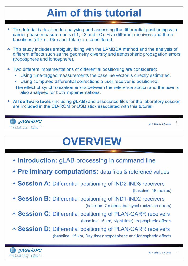
Research group of Astronomy & GeomaticsTechnical University of Catalonia
gAGE/UPC @ J. Sanz & J.M. Juan 3
This tutorial is devoted to analysing and assessing the differential positioning with carrier phase measurements (L1, L2 and LC). Five different receivers and three baselines (of 7m, 18m and 15km) are considered.
This study includes ambiguity fixing with the LAMBDA method and the analysis of different effects such as the geometry diversity and atmospheric propagation errors (troposphere and ionosphere).
Two different implementations of differential positioning are considered:• Using time-tagged measurements the baseline vector is directly estimated.• Using computed differential corrections a user receiver is positioned. The effect of synchronization errors between the reference station and the user is
also analysed for both implementations.
All software tools (including gLAB) and associated files for the laboratory session are included in the CD-ROM or USB stick associated with this tutorial.
Aim of this tutorial
Research group of Astronomy & GeomaticsTechnical University of Catalonia
gAGE/UPC @ J. Sanz & J.M. Juan
Introduction: gLAB processing in command line
Preliminary computations: data files & reference values
Session A: Differential positioning of IND2-IND3 receivers (baseline: 18 metres)
Session B: Differential positioning of IND1-IND2 receivers (baseline: 7 metres, but synchronization errors)
Session C: Differential positioning of PLAN-GARR receivers(baseline: 15 km, Night time): tropospheric effects
Session D: Differential positioning of PLAN-GARR receivers(baseline: 15 km, Day time): tropospheric and Ionospheric effects
OVERVIEW
4
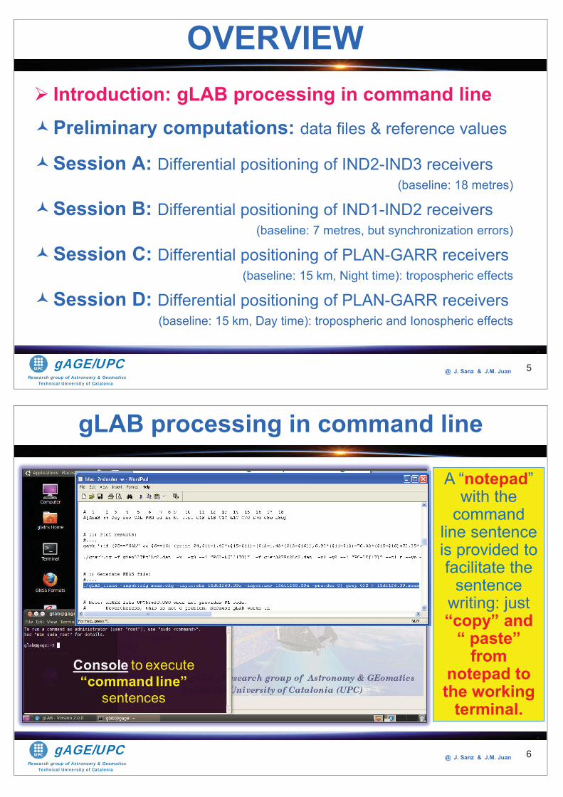
Research group of Astronomy & GeomaticsTechnical University of Catalonia
gAGE/UPC @ J. Sanz & J.M. Juan
Introduction: gLAB processing in command linePreliminary computations: data files & reference values
Session A: Differential positioning of IND2-IND3 receivers (baseline: 18 metres)
Session B: Differential positioning of IND1-IND2 receivers (baseline: 7 metres, but synchronization errors)
Session C: Differential positioning of PLAN-GARR receivers(baseline: 15 km, Night time): tropospheric effects
Session D: Differential positioning of PLAN-GARR receivers(baseline: 15 km, Day time): tropospheric and Ionospheric effects
OVERVIEW
5
Research group of Astronomy & GeomaticsTechnical University of Catalonia
gAGE/UPC @ J. Sanz & J.M. Juan 6
Console to execute “command line”
sentences
A “notepad” with the
command line sentence is provided to facilitate the
sentence writing: just “copy” and
“ paste” from
notepad to the working
terminal.
gLAB processing in command line
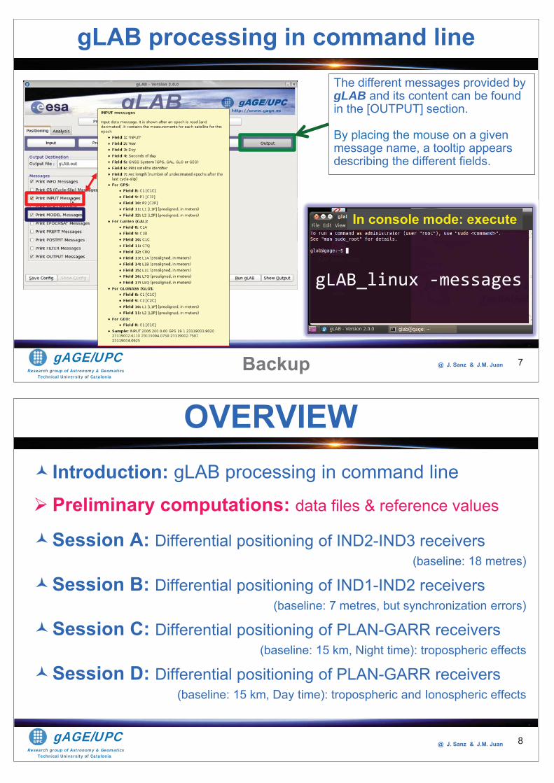
Research group of Astronomy & GeomaticsTechnical University of Catalonia
gAGE/UPC @ J. Sanz & J.M. Juan 7
The different messages provided by gLAB and its content can be found in the [OUTPUT] section.
By placing the mouse on a given message name, a tooltip appears describing the different fields.
Backup
gLAB_linux -messages
In console mode: execute
gLAB processing in command line
Research group of Astronomy & GeomaticsTechnical University of Catalonia
gAGE/UPC @ J. Sanz & J.M. Juan
Introduction: gLAB processing in command line
Preliminary computations: data files & reference values
Session A: Differential positioning of IND2-IND3 receivers (baseline: 18 metres)
Session B: Differential positioning of IND1-IND2 receivers (baseline: 7 metres, but synchronization errors)
Session C: Differential positioning of PLAN-GARR receivers(baseline: 15 km, Night time): tropospheric effects
Session D: Differential positioning of PLAN-GARR receivers(baseline: 15 km, Day time): tropospheric and Ionospheric effects
OVERVIEW
8

Research group of Astronomy & GeomaticsTechnical University of Catalonia
gAGE/UPC @ J. Sanz & J.M. Juan 9
Previous
Preliminary Computations
Research group of Astronomy & GeomaticsTechnical University of Catalonia
gAGE/UPC @ J. Sanz & J.M. Juan 10
This section is devoted to computing the reference values (receivers coordinates) and to preparing the data files to be used in the exercises.
These data files will include the code and carrier measurements and the model components: geometric range, nominal troposphere and ionosphere corrections, satellite elevation and azimuth from each receiver…
This data processing will be done with gLAB for each individual receiver.
This preliminary processing will provide the baseline data files to perform computations easily using basic tools (such as awk for data files handling, to compute Double Differences of measurements) or using octave (MATLAB) scripts for the LAMBDA method implementation.
Detailed guidelines for self learning students are provided in this tutorial and in its associated notepad text file.
P. Preliminary computations
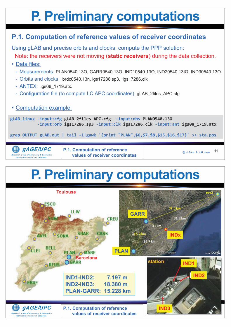
Research group of Astronomy & GeomaticsTechnical University of Catalonia
gAGE/UPC @ J. Sanz & J.M. Juan
P.1. Computation of reference values of receiver coordinatesUsing gLAB and precise orbits and clocks, compute the PPP solution:Note: the receivers were not moving (static receivers) during the data collection.
• Data files: - Measurements: PLAN0540.13O, GARR0540.13O, IND10540.13O, IND20540.13IO, IND30540.13O.- Orbits and clocks: brdc0540.13n, igs17286.sp3, igs17286.clk - ANTEX: igs08_1719.atx.- Configuration file (to compute LC APC coordinates): gLAB_2files_APC.cfg
• Computation example:
11
P. Preliminary computations
gLAB_linux -input:cfg gLAB_2files_APC.cfg -input:obs PLAN0540.13O-input:orb igs17286.sp3 -input:clk igs17286.clk -input:ant igs08_1719.atx
grep OUTPUT gLAB.out | tail -1|gawk '{print "PLAN",$6,$7,$8,$15,$16,$17}' >> sta.pos
P.1. Computation of reference values of receiver coordinates
Research group of Astronomy & GeomaticsTechnical University of Catalonia
gAGE/UPC @ J. Sanz & J.M. Juan 12P.1. Computation of reference
values of receiver coordinates
P. Preliminary computations
@@@@@@@@@@ JJJJJJJ. nannananaaaaSaSaSaSaSaSaSaSaSSaaSSSanaaaSanaSanaaaaSaSSaSaaaaanaaaaaSSaanaannanaSSSSS zzzzzzzz &&&&&&&&&& JJJJJJJ..MM. uaJuaannnnnnnnnnnnnnnnnnnnnnnnnnnnnnnnnnnnnnnnnnn 2222222212221211111112222221121121221212212112221112122122212121222121222112211222222222222122222222222222121212121222212222222222222222222122122222222212222122
PLAN
GARR
INDx
IND1
IND2
IND3
IND1-IND2: 7.197 mIND2-IND3: 18.380 m PLAN-GARR: 15.228 km
Barcelona
Toulouse
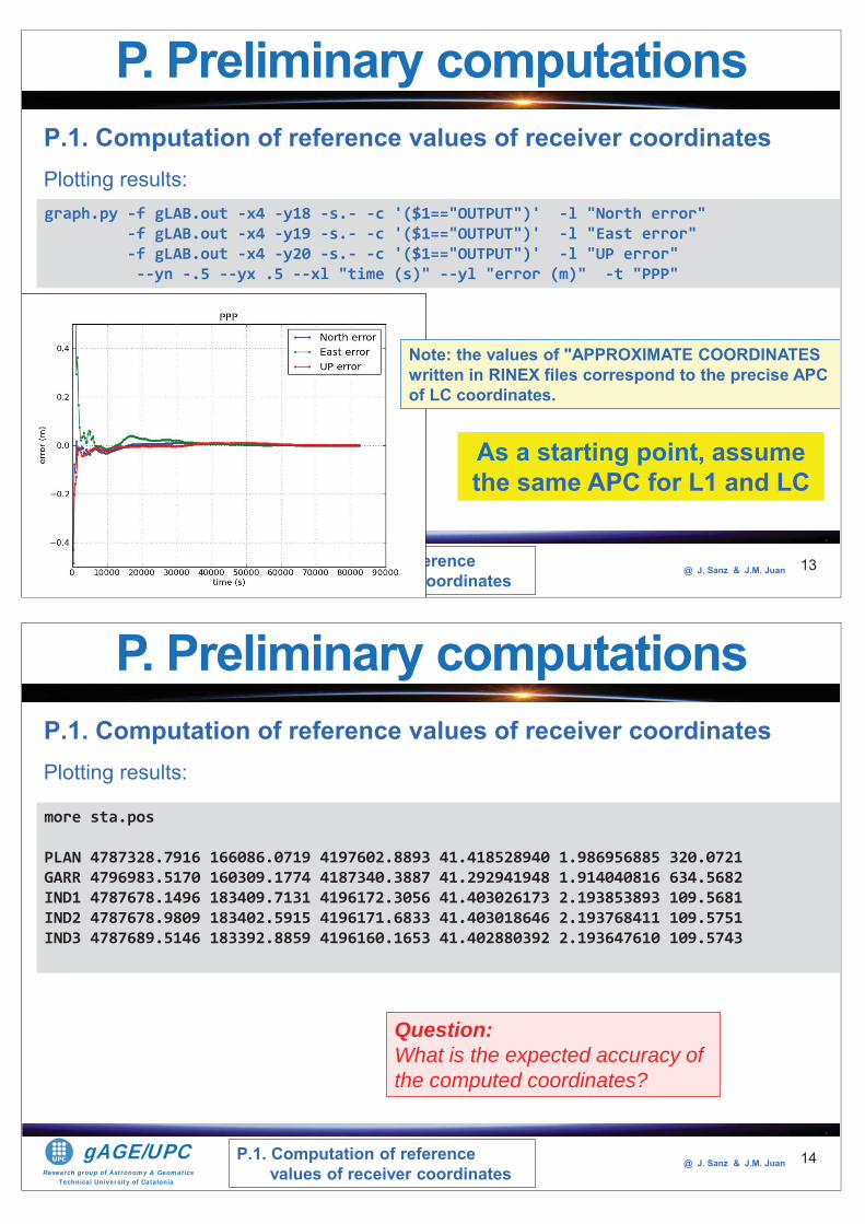
Research group of Astronomy & GeomaticsTechnical University of Catalonia
gAGE/UPC @ J. Sanz & J.M. Juan
P.1. Computation of reference values of receiver coordinates
P.1. Computation of reference values of receiver coordinatesPlotting results:
13
P. Preliminary computations
graph.py -f gLAB.out -x4 -y18 -s.- -c '($1=="OUTPUT")' -l "North error" -f gLAB.out -x4 -y19 -s.- -c '($1=="OUTPUT")' -l "East error" -f gLAB.out -x4 -y20 -s.- -c '($1=="OUTPUT")' -l "UP error" --yn -.5 --yx .5 --xl "time (s)" --yl "error (m)" -t "PPP"
Note: the values of "APPROXIMATE COORDINATES written in RINEX files correspond to the precise APC of LC coordinates.
As a starting point, assume the same APC for L1 and LC
Research group of Astronomy & GeomaticsTechnical University of Catalonia
gAGE/UPC @ J. Sanz & J.M. Juan
P.1. Computation of reference values of receiver coordinatesPlotting results:
14
P. Preliminary computations
more sta.pos
PLAN 4787328.7916 166086.0719 4197602.8893 41.418528940 1.986956885 320.0721GARR 4796983.5170 160309.1774 4187340.3887 41.292941948 1.914040816 634.5682IND1 4787678.1496 183409.7131 4196172.3056 41.403026173 2.193853893 109.5681IND2 4787678.9809 183402.5915 4196171.6833 41.403018646 2.193768411 109.5751IND3 4787689.5146 183392.8859 4196160.1653 41.402880392 2.193647610 109.5743
Question: What is the expected accuracy of the computed coordinates?
P.1. Computation of reference values of receiver coordinates
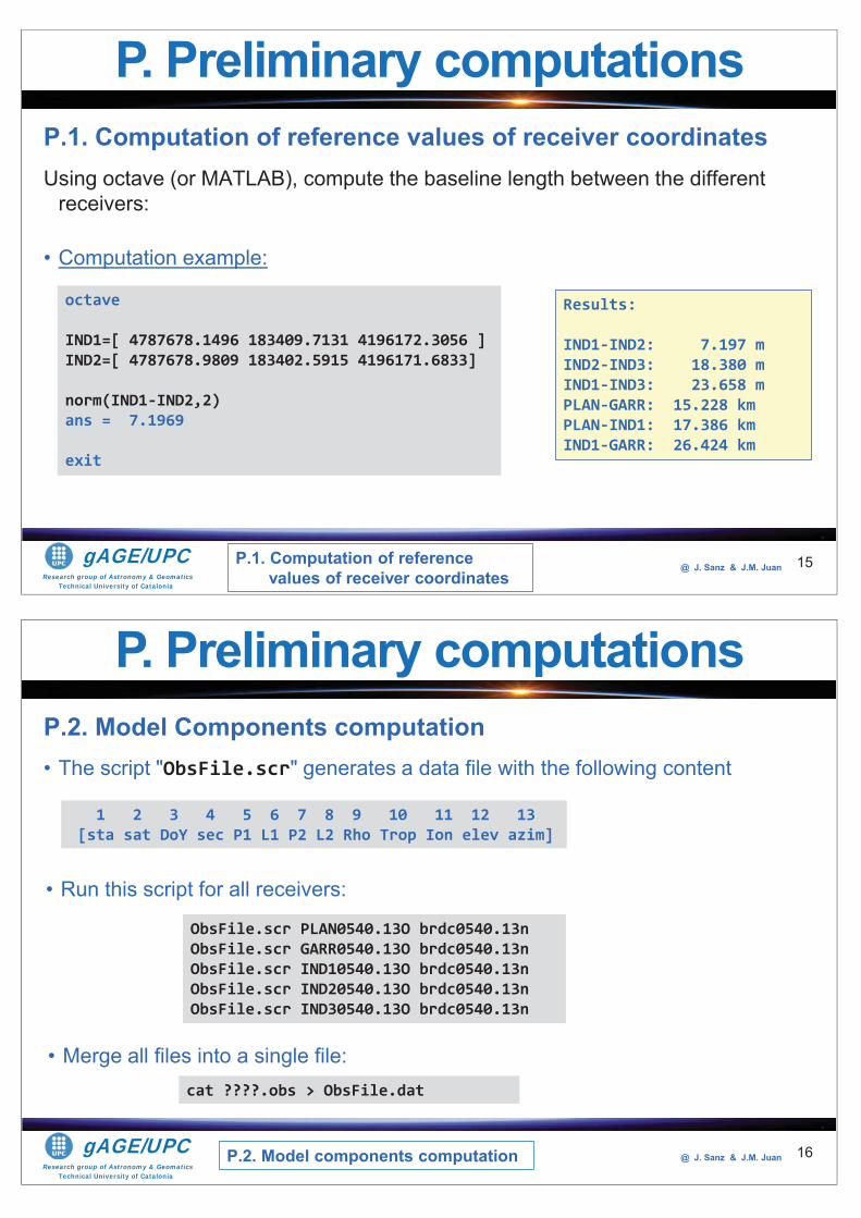
Research group of Astronomy & GeomaticsTechnical University of Catalonia
gAGE/UPC @ J. Sanz & J.M. Juan
P.1. Computation of reference values of receiver coordinatesUsing octave (or MATLAB), compute the baseline length between the different
receivers:
• Computation example:
15
P. Preliminary computations
octave
IND1=[ 4787678.1496 183409.7131 4196172.3056 ]IND2=[ 4787678.9809 183402.5915 4196171.6833]
norm(IND1-IND2,2)ans = 7.1969
exit
Results:
IND1-IND2: 7.197 mIND2-IND3: 18.380 m IND1-IND3: 23.658 m PLAN-GARR: 15.228 kmPLAN-IND1: 17.386 kmIND1-GARR: 26.424 km
P.1. Computation of reference values of receiver coordinates
Research group of Astronomy & GeomaticsTechnical University of Catalonia
gAGE/UPC @ J. Sanz & J.M. Juan
P.2. Model Components computation• The script "ObsFile.scr" generates a data file with the following content
16
P. Preliminary computations
1 2 3 4 5 6 7 8 9 10 11 12 13[sta sat DoY sec P1 L1 P2 L2 Rho Trop Ion elev azim]
• Run this script for all receivers:
ObsFile.scr PLAN0540.13O brdc0540.13nObsFile.scr GARR0540.13O brdc0540.13nObsFile.scr IND10540.13O brdc0540.13nObsFile.scr IND20540.13O brdc0540.13nObsFile.scr IND30540.13O brdc0540.13n
• Merge all files into a single file:cat ????.obs > ObsFile.dat
P.2. Model components computation
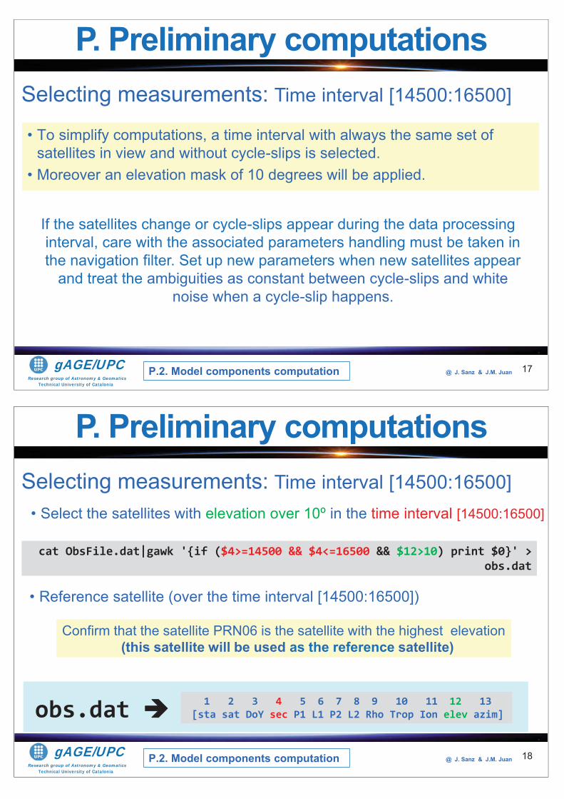
Research group of Astronomy & GeomaticsTechnical University of Catalonia
gAGE/UPC @ J. Sanz & J.M. Juan
• To simplify computations, a time interval with always the same set of satellites in view and without cycle-slips is selected.
• Moreover an elevation mask of 10 degrees will be applied.
17
P. Preliminary computationsSelecting measurements: Time interval [14500:16500]
P.2. Model components computation
If the satellites change or cycle-slips appear during the data processing interval, care with the associated parameters handling must be taken in the navigation filter. Set up new parameters when new satellites appear
and treat the ambiguities as constant between cycle-slips and white noise when a cycle-slip happens.
Research group of Astronomy & GeomaticsTechnical University of Catalonia
gAGE/UPC @ J. Sanz & J.M. Juan
• Select the satellites with elevation over 10º in the time interval [14500:16500]
18
P. Preliminary computations
Confirm that the satellite PRN06 is the satellite with the highest elevation (this satellite will be used as the reference satellite)
cat ObsFile.dat|gawk '{if ($4>=14500 && $4<=16500 && $12>10) print $0}' > obs.dat
• Reference satellite (over the time interval [14500:16500])
Selecting measurements: Time interval [14500:16500]
1 2 3 4 5 6 7 8 9 10 11 12 13[sta sat DoY sec P1 L1 P2 L2 Rho Trop Ion elev azim]obs.dat
P.2. Model components computation
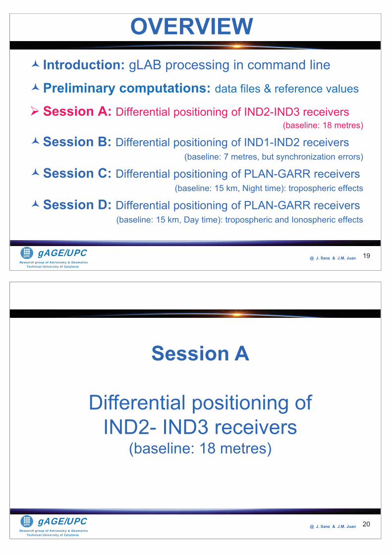
Research group of Astronomy & GeomaticsTechnical University of Catalonia
gAGE/UPC @ J. Sanz & J.M. Juan
Introduction: gLAB processing in command line
Preliminary computations: data files & reference values
Session A: Differential positioning of IND2-IND3 receivers (baseline: 18 metres)
Session B: Differential positioning of IND1-IND2 receivers (baseline: 7 metres, but synchronization errors)
Session C: Differential positioning of PLAN-GARR receivers(baseline: 15 km, Night time): tropospheric effects
Session D: Differential positioning of PLAN-GARR receivers(baseline: 15 km, Day time): tropospheric and Ionospheric effects
OVERVIEW
19
Research group of Astronomy & GeomaticsTechnical University of Catalonia
gAGE/UPC @ J. Sanz & J.M. Juan 20
Session A
Differential positioning of IND2- IND3 receivers
(baseline: 18 metres)
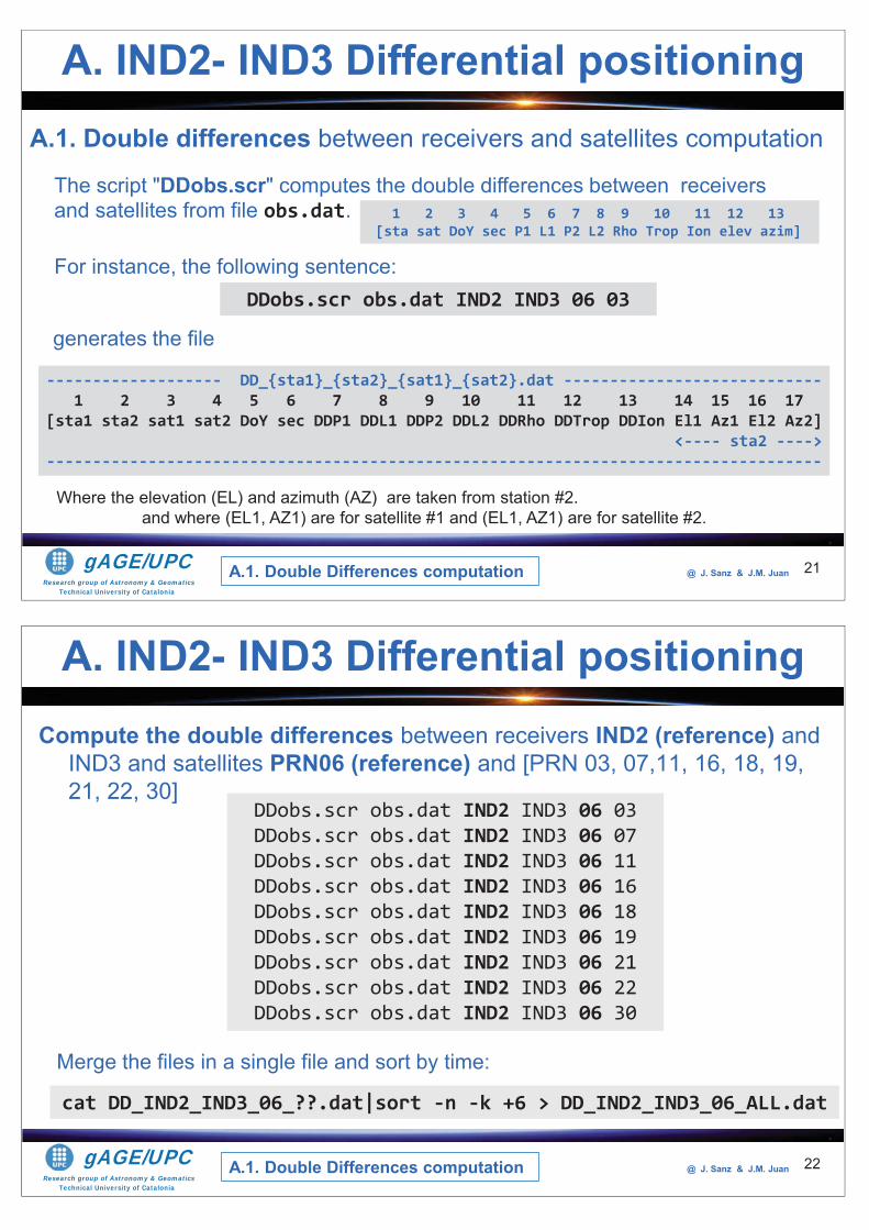
Research group of Astronomy & GeomaticsTechnical University of Catalonia
gAGE/UPC @ J. Sanz & J.M. Juan
A.1. Double differences between receivers and satellites computation
21
A. IND2- IND3 Differential positioning
1 2 3 4 5 6 7 8 9 10 11 12 13[sta sat DoY sec P1 L1 P2 L2 Rho Trop Ion elev azim]
DDobs.scr obs.dat IND2 IND3 06 03
------------------- DD_{sta1}_{sta2}_{sat1}_{sat2}.dat ----------------------------1 2 3 4 5 6 7 8 9 10 11 12 13 14 15 16 17
[sta1 sta2 sat1 sat2 DoY sec DDP1 DDL1 DDP2 DDL2 DDRho DDTrop DDIon El1 Az1 El2 Az2]<---- sta2 ---->
------------------------------------------------------------------------------------
generates the file
Where the elevation (EL) and azimuth (AZ) are taken from station #2.and where (EL1, AZ1) are for satellite #1 and (EL1, AZ1) are for satellite #2.
A.1. Double Differences computation
The script "DDobs.scr" computes the double differences between receivers and satellites from file obs.dat.
For instance, the following sentence:
Research group of Astronomy & GeomaticsTechnical University of Catalonia
gAGE/UPC @ J. Sanz & J.M. Juan
Compute the double differences between receivers IND2 (reference) and IND3 and satellites PRN06 (reference) and [PRN 03, 07,11, 16, 18, 19, 21, 22, 30]
22
A. IND2- IND3 Differential positioning
DDobs.scr obs.dat IND2 IND3 06 03DDobs.scr obs.dat IND2 IND3 06 07DDobs.scr obs.dat IND2 IND3 06 11DDobs.scr obs.dat IND2 IND3 06 16DDobs.scr obs.dat IND2 IND3 06 18DDobs.scr obs.dat IND2 IND3 06 19DDobs.scr obs.dat IND2 IND3 06 21DDobs.scr obs.dat IND2 IND3 06 22DDobs.scr obs.dat IND2 IND3 06 30
Merge the files in a single file and sort by time:
cat DD_IND2_IND3_06_??.dat|sort -n -k +6 > DD_IND2_IND3_06_ALL.dat
A.1. Double Differences computation
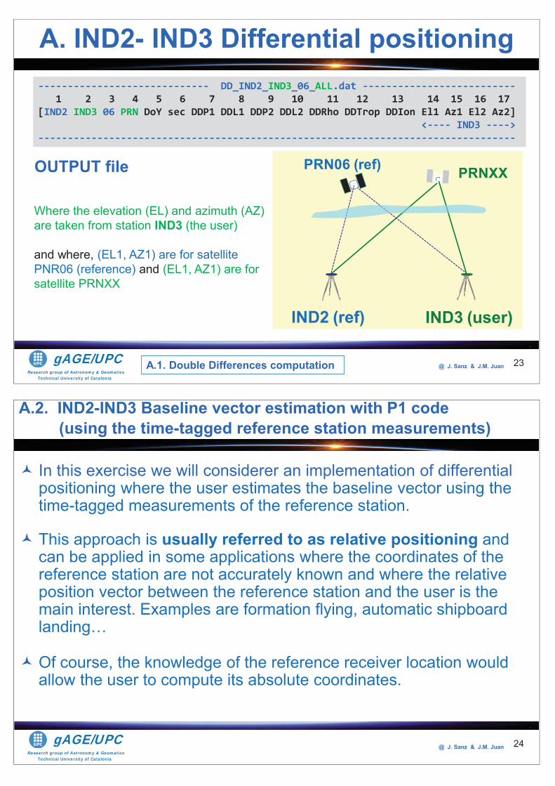
Research group of Astronomy & GeomaticsTechnical University of Catalonia
gAGE/UPC @ J. Sanz & J.M. Juan 23
----------------------------- DD_IND2_IND3_06_ALL.dat --------------------------1 2 3 4 5 6 7 8 9 10 11 12 13 14 15 16 17
[IND2 IND3 06 PRN DoY sec DDP1 DDL1 DDP2 DDL2 DDRho DDTrop DDIon El1 Az1 El2 Az2]<---- IND3 ---->
---------------------------------------------------------------------------------
OUTPUT file
Where the elevation (EL) and azimuth (AZ) are taken from station IND3 (the user)
and where, (EL1, AZ1) are for satellite PNR06 (reference) and (EL1, AZ1) are for satellite PRNXX
IND3 (user)IND2 (ref)
PRN06 (ref) PRNXX
A. IND2- IND3 Differential positioning
A.1. Double Differences computation
Research group of Astronomy & GeomaticsTechnical University of Catalonia
gAGE/UPC @ J. Sanz & J.M. Juan 24
In this exercise we will considerer an implementation of differential positioning where the user estimates the baseline vector using the time-tagged measurements of the reference station.
This approach is usually referred to as relative positioning and can be applied in some applications where the coordinates of the reference station are not accurately known and where the relative position vector between the reference station and the user is the main interest. Examples are formation flying, automatic shipboard landing…
Of course, the knowledge of the reference receiver location would allow the user to compute its absolute coordinates.
A.2. IND2-IND3 Baseline vector estimation with P1 code(using the time-tagged reference station measurements)
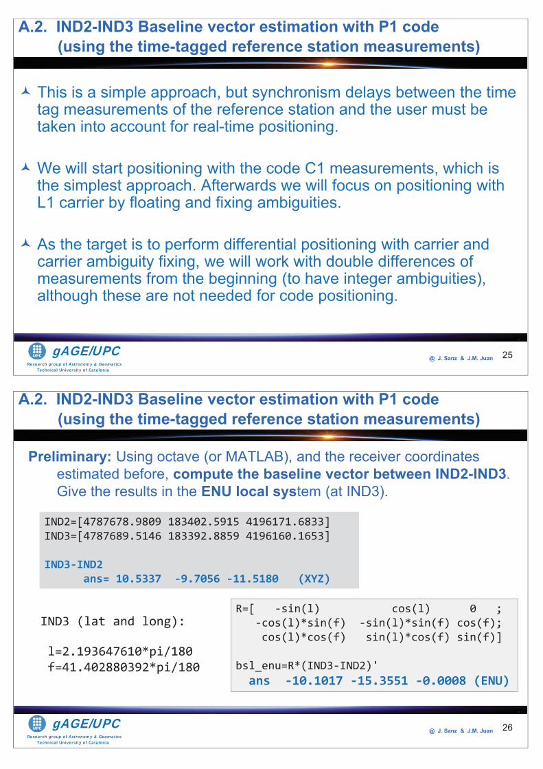
Research group of Astronomy & GeomaticsTechnical University of Catalonia
gAGE/UPC @ J. Sanz & J.M. Juan 25
This is a simple approach, but synchronism delays between the time tag measurements of the reference station and the user must be taken into account for real-time positioning.
We will start positioning with the code C1 measurements, which is the simplest approach. Afterwards we will focus on positioning with L1 carrier by floating and fixing ambiguities.
As the target is to perform differential positioning with carrier and carrier ambiguity fixing, we will work with double differences of measurements from the beginning (to have integer ambiguities), although these are not needed for code positioning.
A.2. IND2-IND3 Baseline vector estimation with P1 code(using the time-tagged reference station measurements)
Research group of Astronomy & GeomaticsTechnical University of Catalonia
gAGE/UPC @ J. Sanz & J.M. Juan
Preliminary: Using octave (or MATLAB), and the receiver coordinates estimated before, compute the baseline vector between IND2-IND3. Give the results in the ENU local system (at IND3).
26
IND2=[4787678.9809 183402.5915 4196171.6833]IND3=[4787689.5146 183392.8859 4196160.1653]
IND3-IND2ans= 10.5337 -9.7056 -11.5180 (XYZ)
R=[ -sin(l) cos(l) 0 ; -cos(l)*sin(f) -sin(l)*sin(f) cos(f); cos(l)*cos(f) sin(l)*cos(f) sin(f)]
bsl_enu=R*(IND3-IND2)' ans -10.1017 -15.3551 -0.0008 (ENU)
IND3 (lat and long):
l=2.193647610*pi/180f=41.402880392*pi/180
A.2. IND2-IND3 Baseline vector estimation with P1 code(using the time-tagged reference station measurements)
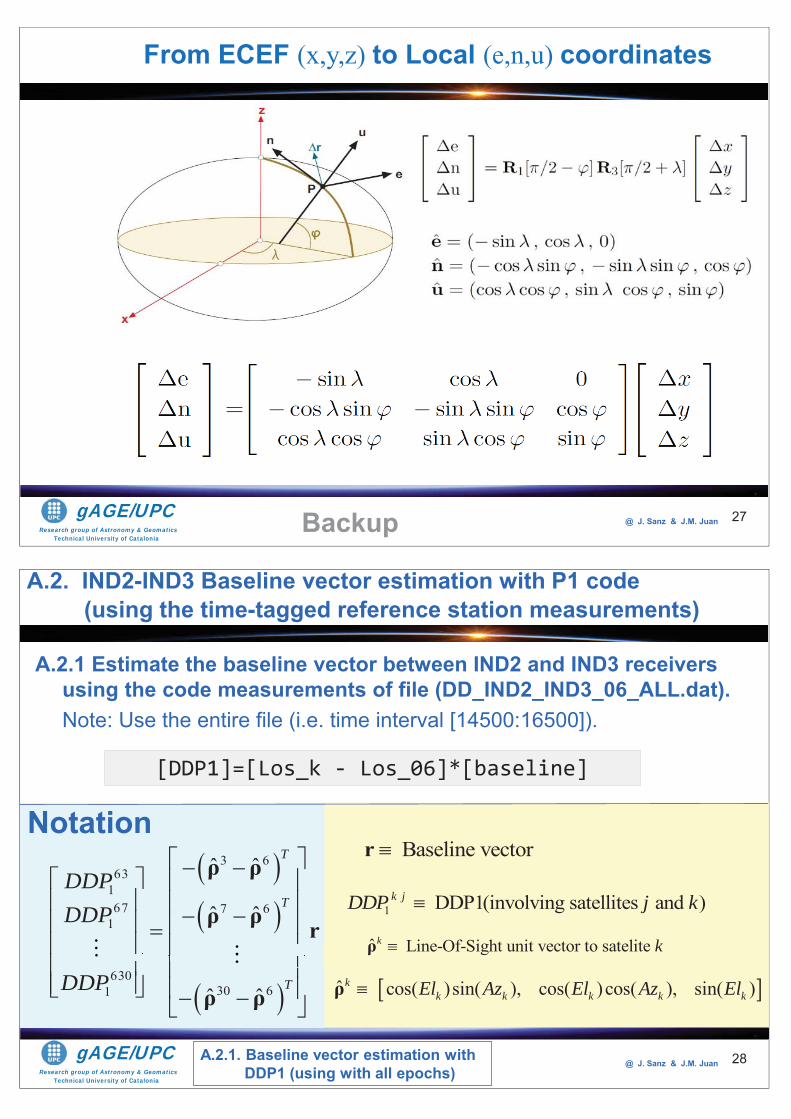
Research group of Astronomy & GeomaticsTechnical University of Catalonia
gAGE/UPC @ J. Sanz & J.M. Juan 27
From ECEF (x,y,z) to Local (e,n,u) coordinates
Backup
Research group of Astronomy & GeomaticsTechnical University of Catalonia
gAGE/UPC @ J. Sanz & J.M. Juan
A.2.1 Estimate the baseline vector between IND2 and IND3 receivers using the code measurements of file (DD_IND2_IND3_06_ALL.dat). Note: Use the entire file (i.e. time interval [14500:16500]).
28
[DDP1]=[Los_k - Los_06]*[baseline]
3 663
167 7 6
1
63030 61
ˆ ˆ
ˆ ˆ
ˆ ˆ
T
T
T
DDPDDP
DDP
ρ ρ
ρ ρ r
ρ ρ
1 DDP1(involving satellites and )k jDDP j k
ˆ Line-Of-Sight unit vector to satelite k kρ
ˆ cos( )sin( ), cos( )cos( ), sin( )kk k k k kEl Az El Az Elρ
Baseline vectorrNotation
A.2.1. Baseline vector estimation with DDP1 (using with all epochs)
A.2. IND2-IND3 Baseline vector estimation with P1 code(using the time-tagged reference station measurements)
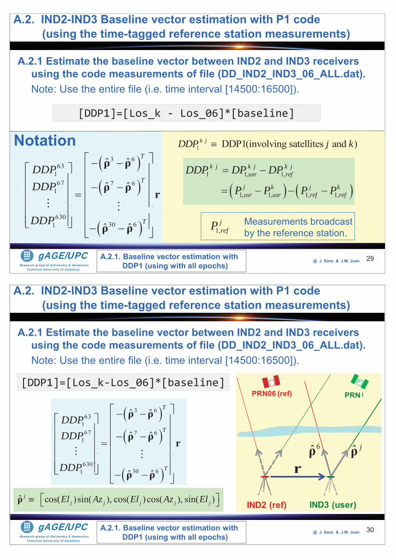
Research group of Astronomy & GeomaticsTechnical University of Catalonia
gAGE/UPC @ J. Sanz & J.M. Juan
A.2.1 Estimate the baseline vector between IND2 and IND3 receivers using the code measurements of file (DD_IND2_IND3_06_ALL.dat). Note: Use the entire file (i.e. time interval [14500:16500]).
29
[DDP1]=[Los_k - Los_06]*[baseline]
3 663
167 7 6
1
63030 61
ˆ ˆ
ˆ ˆ
ˆ ˆ
T
T
T
DDPDDP
DDP
ρ ρ
ρ ρ r
ρ ρ
1 DDP1(involving satellites and )k jDDP j kNotation
A.2.1. Baseline vector estimation with DDP1 (using with all epochs)
A.2. IND2-IND3 Baseline vector estimation with P1 code(using the time-tagged reference station measurements)
1 1, 1,
1, 1, 1, 1,
k j k j k jusr ref
j k j kusr usr ref ref
DDP DP DP
P P P P
1,jrefP Measurements broadcast
by the reference station.
Research group of Astronomy & GeomaticsTechnical University of Catalonia
gAGE/UPC @ J. Sanz & J.M. Juan
IND3 (user)IND2 (ref)
PRN06 (ref) PRN j
A.2.1 Estimate the baseline vector between IND2 and IND3 receivers using the code measurements of file (DD_IND2_IND3_06_ALL.dat). Note: Use the entire file (i.e. time interval [14500:16500]).
30
3 663
167 7 6
1
63030 61
ˆ ˆ
ˆ ˆ
ˆ ˆ
T
T
T
DDPDDP
DDP
ρ ρ
ρ ρ r
ρ ρ
6ρ ˆ jρr
A.2. IND2-IND3 Baseline vector estimation with P1 code(using the time-tagged reference station measurements)
A.2.1. Baseline vector estimation with DDP1 (using with all epochs)
[DDP1]=[Los_k-Los_06]*[baseline]
ˆ cos( )sin( ), cos( )cos( ), sin( )jj j j j jEl Az El Az Elρ
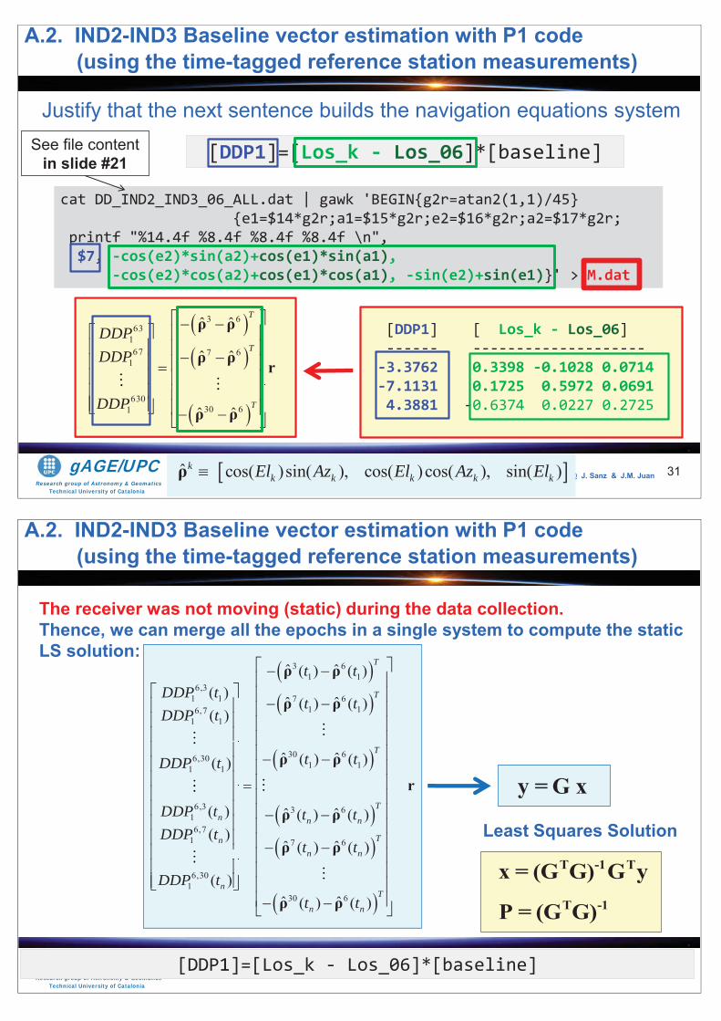
Research group of Astronomy & GeomaticsTechnical University of Catalonia
gAGE/UPC @ J. Sanz & J.M. Juan 31
cat DD_IND2_IND3_06_ALL.dat | gawk 'BEGIN{g2r=atan2(1,1)/45} {e1=$14*g2r;a1=$15*g2r;e2=$16*g2r;a2=$17*g2r;
printf "%14.4f %8.4f %8.4f %8.4f \n",$7, -cos(e2)*sin(a2)+cos(e1)*sin(a1),
-cos(e2)*cos(a2)+cos(e1)*cos(a1), -sin(e2)+sin(e1)}' > M.dat
Justify that the next sentence builds the navigation equations system
[DDP1]=[Los_k - Los_06]*[baseline]
[DDP1] [ Los_k - Los_06] ------ ---------------------3.3762 0.3398 -0.1028 0.0714-7.1131 0.1725 0.5972 0.0691 4.3881 -0.6374 0.0227 0.2725
3 663
167 7 6
1
63030 61
ˆ ˆ
ˆ ˆ
ˆ ˆ
T
T
T
DDPDDP
DDP
ρ ρ
ρ ρ r
ρ ρ
ˆ cos( )sin( ), cos( )cos( ), sin( )kk k k k kEl Az El Az Elρ
A.2. IND2-IND3 Baseline vector estimation with P1 code(using the time-tagged reference station measurements)
See file content in slide #21
Research group of Astronomy & GeomaticsTechnical University of Catalonia
gAGE/UPC @ J. Sanz & J.M. Juan 32[DDP1]=[Los_k - Los_06]*[baseline]
3 61 1
6,31 1 7 6
1 16,71 1
30 66,301 11 1
6,3 3 616,7
1 7 6
6,301
30
ˆ ˆ( ) ( )( ) ˆ ˆ( ) ( )( )
ˆ ˆ( ) ( )( )
( ) ˆ ˆ( ) ( )( )
ˆ ˆ( ) ( )
( )ˆ ( )
T
T
T
Tn n n
Tnn n
n
n
t tDDP t
t tDDP t
t tDDP t
DDP t t tDDP t
t t
DDP tt
ρ ρ
ρ ρ
ρ ρ
ρ ρ
ρ ρ
ρ 6ˆ ( )T
nt
r
ρ
The receiver was not moving (static) during the data collection. Thence, we can merge all the epochs in a single system to compute the static LS solution:
y =G x
T -1 Tx = (G G) G yT -1P = (G G)
Least Squares Solution
A.2. IND2-IND3 Baseline vector estimation with P1 code(using the time-tagged reference station measurements)
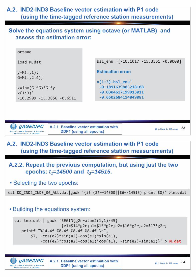
Research group of Astronomy & GeomaticsTechnical University of Catalonia
gAGE/UPC @ J. Sanz & J.M. Juan
Solve the equations system using octave (or MATLAB) and assess the estimation error:
33
octave
load M.dat
y=M(:,1);G=M(:,2:4);
x=inv(G'*G)*G'*yx(1:3)'-10.2909 -15.3856 -0.6511
bsl_enu =[-10.1017 -15.3551 -0.0008]
Estimation error:
x(1:3)-bsl_enu'-0.1891639885218108-0.0304617199913011-0.6502684114849081
A.2. IND2-IND3 Baseline vector estimation with P1 code(using the time-tagged reference station measurements)
A.2.1. Baseline vector estimation with DDP1 (using all epochs)
Research group of Astronomy & GeomaticsTechnical University of Catalonia
gAGE/UPC @ J. Sanz & J.M. Juan
A.2.2. Repeat the previous computation, but using just the two epochs: t1=14500 and t2=14515.
34
cat DD_IND2_IND3_06_ALL.dat|gawk '{if ($6==14500||$6==14515) print $0}‘ >tmp.dat
• Selecting the two epochs:
cat tmp.dat | gawk 'BEGIN{g2r=atan2(1,1)/45} {e1=$14*g2r;a1=$15*g2r;e2=$16*g2r;a2=$17*g2r;
printf "%14.4f %8.4f %8.4f %8.4f \n",$7, -cos(e2)*sin(a2)+cos(e1)*sin(a1),
-cos(e2)*cos(a2)+cos(e1)*cos(a1), -sin(e2)+sin(e1)}' > M.dat
• Building the equations system:
A.2. IND2-IND3 Baseline vector estimation with P1 code(using the time-tagged reference station measurements)
A.2.1. Baseline vector estimation with DDP1 (using all epochs)
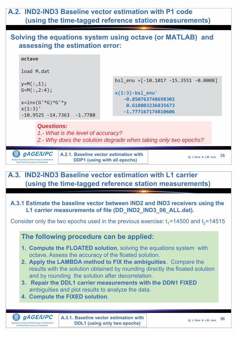
Research group of Astronomy & GeomaticsTechnical University of Catalonia
gAGE/UPC @ J. Sanz & J.M. Juan
Solving the equations system using octave (or MATLAB) and assessing the estimation error:
35
octave
load M.dat
y=M(:,1);G=M(:,2:4);
x=inv(G'*G)*G'*yx(1:3)'-10.9525 -14.7363 -1.7780
bsl_enu =[-10.1017 -15.3551 -0.0008]
x(1:3)-bsl_enu'-0.8507637486983020.618803236835673-1.777167174810606
Questions:1.- What is the level of accuracy?2.- Why does the solution degrade when taking only two epochs?
A.2. IND2-IND3 Baseline vector estimation with P1 code(using the time-tagged reference station measurements)
A.2.1. Baseline vector estimation with DDP1 (using with all epochs)
Research group of Astronomy & GeomaticsTechnical University of Catalonia
gAGE/UPC @ J. Sanz & J.M. Juan 36
A.3.1 Estimate the baseline vector between IND2 and IND3 receivers using the L1 carrier measurements of file (DD_IND2_IND3_06_ALL.dat).
Consider only the two epochs used in the previous exercise: t1=14500 and t2=14515
The following procedure can be applied:1. Compute the FLOATED solution, solving the equations system with
octave. Assess the accuracy of the floated solution.2. Apply the LAMBDA method to FIX the ambiguities. Compare the
results with the solution obtained by rounding directly the floated solution and by rounding the solution after decorrelation.
3. Repair the DDL1 carrier measurements with the DDN1 FIXED ambiguities and plot results to analyze the data.
4. Compute the FIXED solution.
A.3.1. Baseline vector estimation with DDL1 (using only two epochs)
A.3. IND2-IND3 Baseline vector estimation with L1 carrier(using the time-tagged reference station measurements)
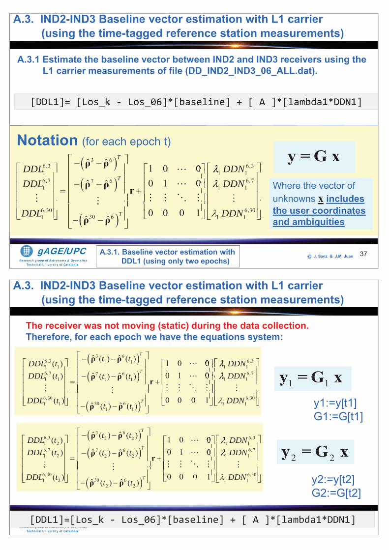
Research group of Astronomy & GeomaticsTechnical University of Catalonia
gAGE/UPC @ J. Sanz & J.M. Juan
A.3.1 Estimate the baseline vector between IND2 and IND3 receivers using the L1 carrier measurements of file (DD_IND2_IND3_06_ALL.dat).
37
[DDL1]= [Los_k - Los_06]*[baseline] + [ A ]*[lambda1*DDN1]
3 66,3 6,31 1 16,7 6,77 61 1 1
6,30 6,3030 61 1 1
ˆ ˆ 1 0 00 1 0ˆ ˆ
0 0 0 1ˆ ˆ
00
T
T
T
DDL DDNDDL DDN
DDL DDN
ρ ρ
ρ ρ r
ρ ρ
Notation (for each epoch t)
Where the vector of unknowns x includes the user coordinates and ambiguities
y =G x
A.3. IND2-IND3 Baseline vector estimation with L1 carrier(using the time-tagged reference station measurements)
A.3.1. Baseline vector estimation with DDL1 (using only two epochs)
Research group of Astronomy & GeomaticsTechnical University of Catalonia
gAGE/UPC @ J. Sanz & J.M. Juan 38[DDL1]=[Los_k - Los_06]*[baseline] + [ A ]*[lambda1*DDN1]
3 66,3 6,31 11 1 1 16,7 6,77 61 1 1 11 1
6,30 6,3030 61 1 1 1
1 1
ˆ ˆ( ) ( ) 1 0 0( )0 1 0ˆ ˆ( ) ( ) ( )
0 0 0 1( ) ˆ ˆ( ) ( )
00
T
T
T
t tDDL t DDNDDL t DDNt t
DDL t DDNt t
ρ ρ
ρ ρ r
ρ ρ
3 66,3 6,32 21 2 1 16,7 6,77 61 2 1 12 2
6,30 6,3030 61 2 1 1
2 2
ˆ ˆ( ) ( ) 1 0 0( )0 1 0ˆ ˆ( ) ( ) ( )
0 0 0 1( ) ˆ ˆ( ) ( )
00
T
T
T
t tDDL t DDNDDL t DDNt t
DDL t DDNt t
ρ ρ
ρ ρ r
ρ ρ
1 1y =G xy1:=y[t1] G1:=G[t1]
2 2y = G xy2:=y[t2] G2:=G[t2]
The receiver was not moving (static) during the data collection. Therefore, for each epoch we have the equations system:
A.3. IND2-IND3 Baseline vector estimation with L1 carrier(using the time-tagged reference station measurements)
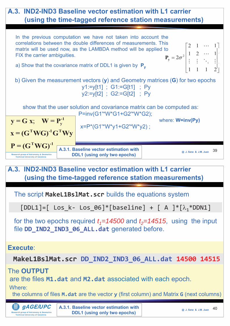
Research group of Astronomy & GeomaticsTechnical University of Catalonia
gAGE/UPC @ J. Sanz & J.M. Juan 39
In the previous computation we have not taken into account thecorrelations between the double differences of measurements. Thismatrix will be used now, as the LAMBDA method will be applied toFIX the carrier ambiguities.
a) Show that the covariance matrix of DDL1 is given by Py
2
2 1 11 2 1
2
1 1 1 2
1111
yP
b) Given the measurement vectors (y) and Geometry matrices (G) for two epochsy1:=y[t1] ; G1:=G[t1] ; Pyy2:=y[t2] ; G2:=G[t2] ; Py
show that the user solution and covariance matrix can be computed as:P=inv(G1'*W*G1+G2'*W*G2);
where: W=inv(Py)x=P*(G1'*W*y1+G2'*W*y2) ;
; -1yy = G x W = P
T -1 Tx = (G WG) G WyT -1P = (G WG)
A.3. IND2-IND3 Baseline vector estimation with L1 carrier(using the time-tagged reference station measurements)
A.3.1. Baseline vector estimation with DDL1 (using only two epochs)
Research group of Astronomy & GeomaticsTechnical University of Catalonia
gAGE/UPC @ J. Sanz & J.M. Juan 40
The script MakeL1BslMat.scr builds the equations system
The OUTPUTare the files M1.dat and M2.dat associated with each epoch.
for the two epochs required t1=14500 and t2=14515, using the input file DD_IND2_IND3_06_ALL.dat generated before.
[DDL1]=[ Los_k- Los_06]*[baseline] + [ A ]*[ 1*DDN1]
MakeL1BslMat.scr DD_IND2_IND3_06_ALL.dat 14500 14515Execute:
Where: the columns of files M.dat are the vector y (first column) and Matrix G (next columns)
A.3. IND2-IND3 Baseline vector estimation with L1 carrier(using the time-tagged reference station measurements)
A.3.1. Baseline vector estimation with DDL1 (using only two epochs)
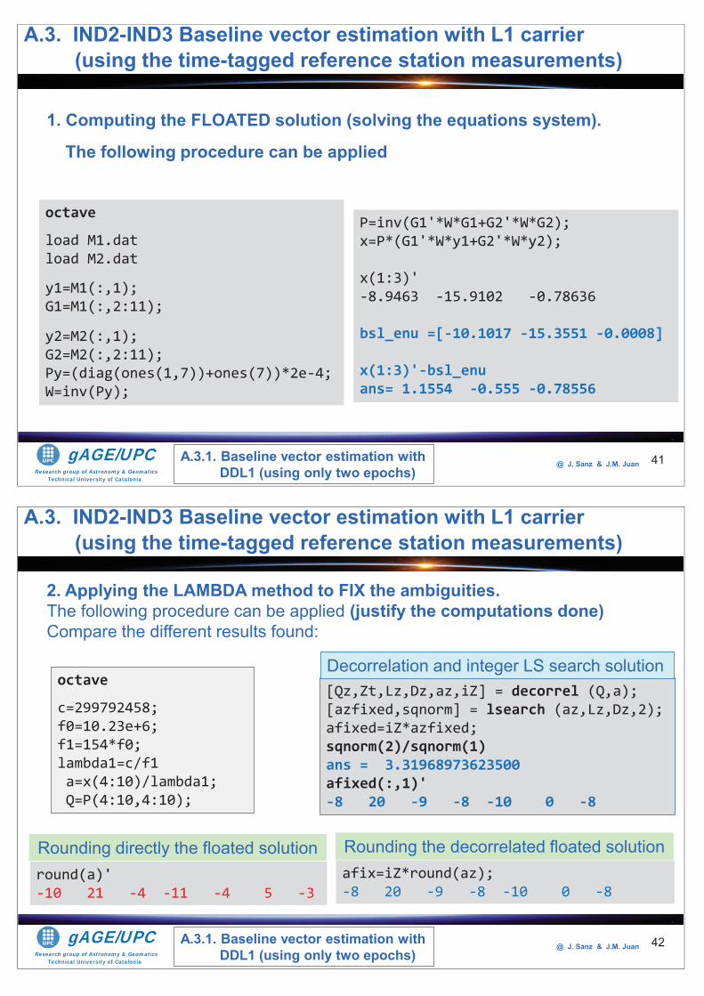
Research group of Astronomy & GeomaticsTechnical University of Catalonia
gAGE/UPC @ J. Sanz & J.M. Juan 41
1. Computing the FLOATED solution (solving the equations system).
The following procedure can be applied
octave
load M1.datload M2.dat
y1=M1(:,1);G1=M1(:,2:11);
y2=M2(:,1);G2=M2(:,2:11);Py=(diag(ones(1,7))+ones(7))*2e-4;W=inv(Py);
P=inv(G1'*W*G1+G2'*W*G2);x=P*(G1'*W*y1+G2'*W*y2);
x(1:3)'-8.9463 -15.9102 -0.78636
bsl_enu =[-10.1017 -15.3551 -0.0008]
x(1:3)'-bsl_enuans= 1.1554 -0.555 -0.78556
A.3. IND2-IND3 Baseline vector estimation with L1 carrier(using the time-tagged reference station measurements)
A.3.1. Baseline vector estimation with DDL1 (using only two epochs)
Research group of Astronomy & GeomaticsTechnical University of Catalonia
gAGE/UPC @ J. Sanz & J.M. Juan 42
2. Applying the LAMBDA method to FIX the ambiguities. The following procedure can be applied (justify the computations done)Compare the different results found:
octave
c=299792458;f0=10.23e+6;f1=154*f0;lambda1=c/f1a=x(4:10)/lambda1;Q=P(4:10,4:10);
afix=iZ*round(az);-8 20 -9 -8 -10 0 -8
[Qz,Zt,Lz,Dz,az,iZ] = decorrel (Q,a);[azfixed,sqnorm] = lsearch (az,Lz,Dz,2);afixed=iZ*azfixed;sqnorm(2)/sqnorm(1)ans = 3.31968973623500afixed(:,1)'-8 20 -9 -8 -10 0 -8
Rounding the decorrelated floated solutionround(a)'-10 21 -4 -11 -4 5 -3
Rounding directly the floated solution
Decorrelation and integer LS search solution
A.3. IND2-IND3 Baseline vector estimation with L1 carrier(using the time-tagged reference station measurements)
A.3.1. Baseline vector estimation with DDL1 (using only two epochs)
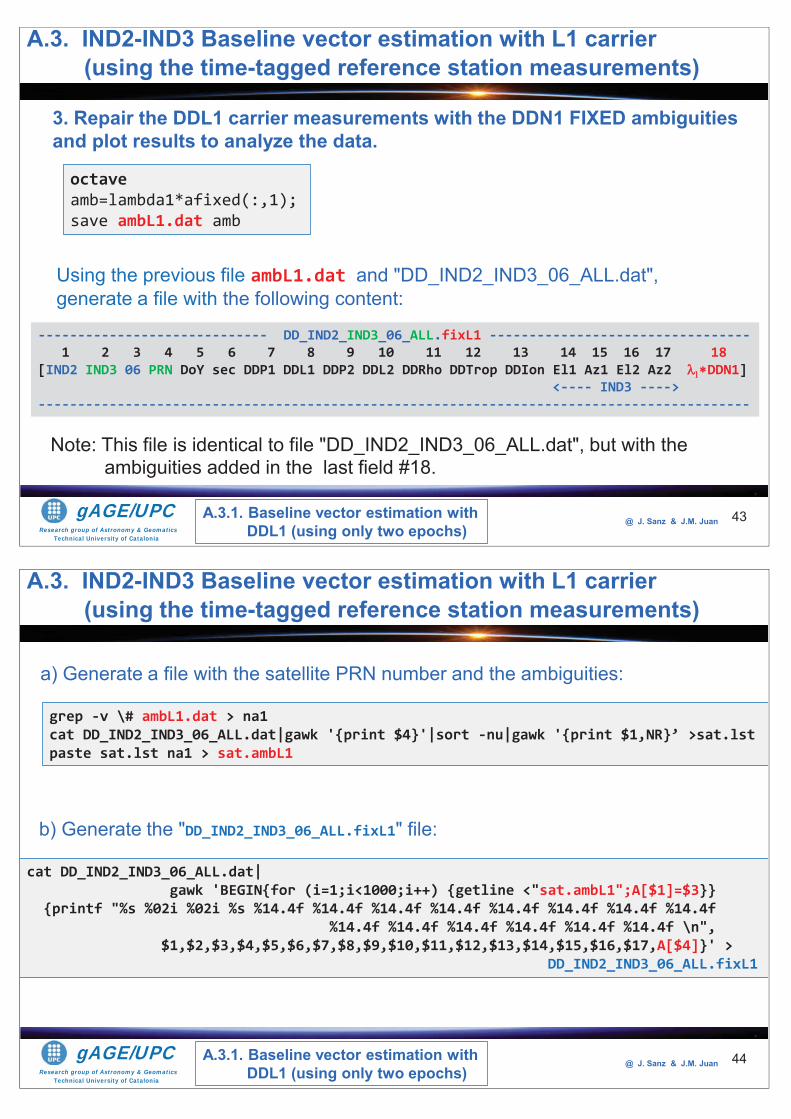
Research group of Astronomy & GeomaticsTechnical University of Catalonia
gAGE/UPC @ J. Sanz & J.M. Juan 43
3. Repair the DDL1 carrier measurements with the DDN1 FIXED ambiguities and plot results to analyze the data.
octaveamb=lambda1*afixed(:,1);save ambL1.dat amb
Using the previous file ambL1.dat and "DD_IND2_IND3_06_ALL.dat",generate a file with the following content:
----------------------------- DD_IND2_IND3_06_ALL.fixL1 ---------------------------------1 2 3 4 5 6 7 8 9 10 11 12 13 14 15 16 17 18
[IND2 IND3 06 PRN DoY sec DDP1 DDL1 DDP2 DDL2 DDRho DDTrop DDIon El1 Az1 El2 Az2 DDN1]<---- IND3 ---->
------------------------------------------------------------------------------------------
Note: This file is identical to file "DD_IND2_IND3_06_ALL.dat", but with the ambiguities added in the last field #18.
A.3. IND2-IND3 Baseline vector estimation with L1 carrier(using the time-tagged reference station measurements)
A.3.1. Baseline vector estimation with DDL1 (using only two epochs)
Research group of Astronomy & GeomaticsTechnical University of Catalonia
gAGE/UPC @ J. Sanz & J.M. Juan 44
grep -v \# ambL1.dat > na1cat DD_IND2_IND3_06_ALL.dat|gawk '{print $4}'|sort -nu|gawk '{print $1,NR}’ >sat.lstpaste sat.lst na1 > sat.ambL1
a) Generate a file with the satellite PRN number and the ambiguities:
cat DD_IND2_IND3_06_ALL.dat|gawk 'BEGIN{for (i=1;i<1000;i++) {getline <"sat.ambL1";A[$1]=$3}}
{printf "%s %02i %02i %s %14.4f %14.4f %14.4f %14.4f %14.4f %14.4f %14.4f %14.4f %14.4f %14.4f %14.4f %14.4f %14.4f %14.4f \n",
$1,$2,$3,$4,$5,$6,$7,$8,$9,$10,$11,$12,$13,$14,$15,$16,$17,A[$4]}' > DD_IND2_IND3_06_ALL.fixL1
b) Generate the "DD_IND2_IND3_06_ALL.fixL1" file:
A.3. IND2-IND3 Baseline vector estimation with L1 carrier(using the time-tagged reference station measurements)
A.3.1. Baseline vector estimation with DDL1 (using only two epochs)
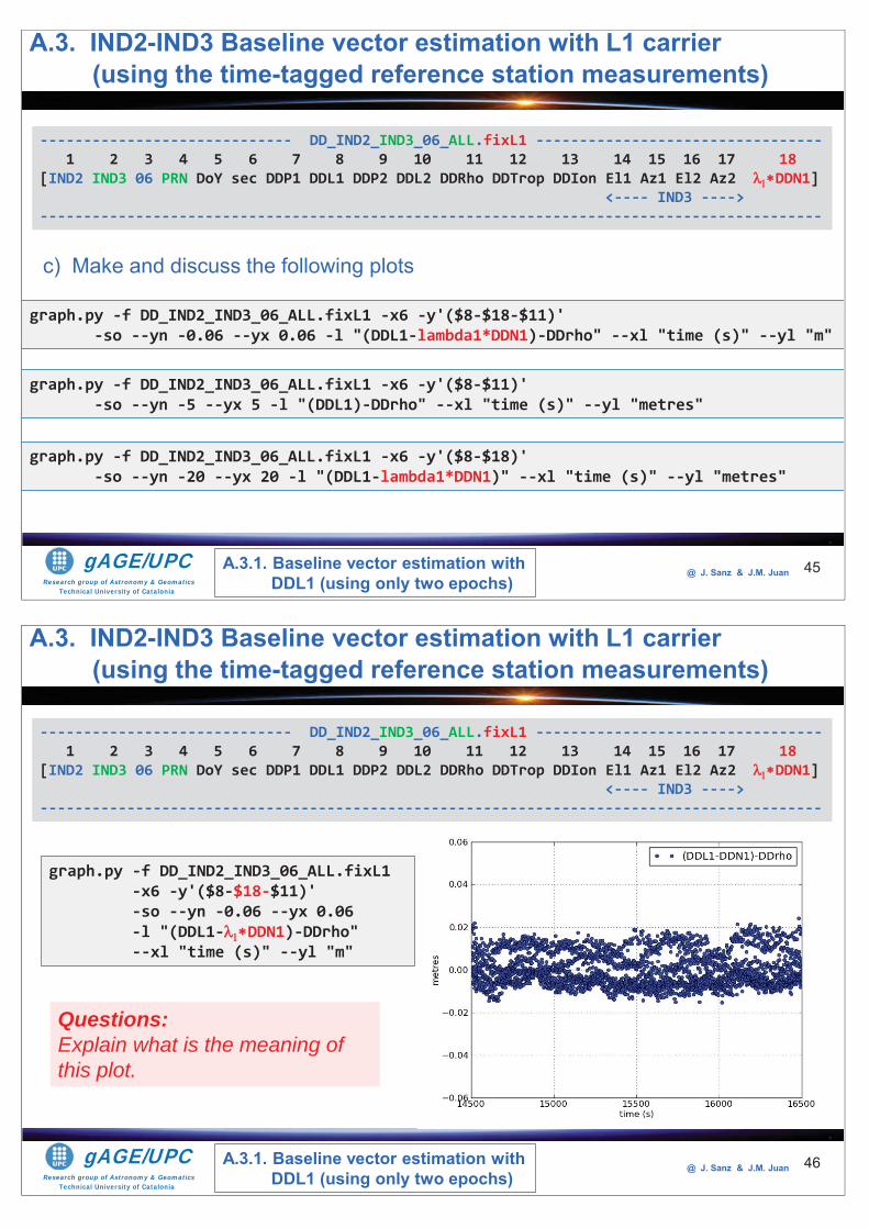
Research group of Astronomy & GeomaticsTechnical University of Catalonia
gAGE/UPC @ J. Sanz & J.M. Juan 45
graph.py -f DD_IND2_IND3_06_ALL.fixL1 -x6 -y'($8-$18-$11)' -so --yn -0.06 --yx 0.06 -l "(DDL1-lambda1*DDN1)-DDrho" --xl "time (s)" --yl "m"
c) Make and discuss the following plots
----------------------------- DD_IND2_IND3_06_ALL.fixL1 ---------------------------------1 2 3 4 5 6 7 8 9 10 11 12 13 14 15 16 17 18
[IND2 IND3 06 PRN DoY sec DDP1 DDL1 DDP2 DDL2 DDRho DDTrop DDIon El1 Az1 El2 Az2 DDN1]<---- IND3 ---->
------------------------------------------------------------------------------------------
graph.py -f DD_IND2_IND3_06_ALL.fixL1 -x6 -y'($8-$11)' -so --yn -5 --yx 5 -l "(DDL1)-DDrho" --xl "time (s)" --yl "metres"
graph.py -f DD_IND2_IND3_06_ALL.fixL1 -x6 -y'($8-$18)' -so --yn -20 --yx 20 -l "(DDL1-lambda1*DDN1)" --xl "time (s)" --yl "metres"
A.3. IND2-IND3 Baseline vector estimation with L1 carrier(using the time-tagged reference station measurements)
A.3.1. Baseline vector estimation with DDL1 (using only two epochs)
Research group of Astronomy & GeomaticsTechnical University of Catalonia
gAGE/UPC @ J. Sanz & J.M. Juan 46
graph.py -f DD_IND2_IND3_06_ALL.fixL1 -x6 -y'($8-$18-$11)' -so --yn -0.06 --yx 0.06 -l "(DDL1- DDN1)-DDrho" --xl "time (s)" --yl "m"
----------------------------- DD_IND2_IND3_06_ALL.fixL1 ---------------------------------1 2 3 4 5 6 7 8 9 10 11 12 13 14 15 16 17 18
[IND2 IND3 06 PRN DoY sec DDP1 DDL1 DDP2 DDL2 DDRho DDTrop DDIon El1 Az1 El2 Az2 DDN1]<---- IND3 ---->
------------------------------------------------------------------------------------------
A.3. IND2-IND3 Baseline vector estimation with L1 carrier(using the time-tagged reference station measurements)
A.3.1. Baseline vector estimation with DDL1 (using only two epochs)
Questions:Explain what is the meaning of this plot.
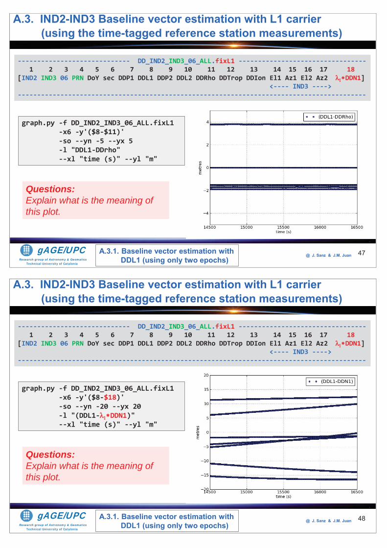
Research group of Astronomy & GeomaticsTechnical University of Catalonia
gAGE/UPC @ J. Sanz & J.M. Juan 47
graph.py -f DD_IND2_IND3_06_ALL.fixL1 -x6 -y'($8-$11)' -so --yn -5 --yx 5 -l "DDL1-DDrho" --xl "time (s)" --yl "m"
----------------------------- DD_IND2_IND3_06_ALL.fixL1 ---------------------------------1 2 3 4 5 6 7 8 9 10 11 12 13 14 15 16 17 18
[IND2 IND3 06 PRN DoY sec DDP1 DDL1 DDP2 DDL2 DDRho DDTrop DDIon El1 Az1 El2 Az2 DDN1]<---- IND3 ---->
------------------------------------------------------------------------------------------
A.3. IND2-IND3 Baseline vector estimation with L1 carrier(using the time-tagged reference station measurements)
A.3.1. Baseline vector estimation with DDL1 (using only two epochs)
Questions:Explain what is the meaning of this plot.
Research group of Astronomy & GeomaticsTechnical University of Catalonia
gAGE/UPC @ J. Sanz & J.M. Juan 48
graph.py -f DD_IND2_IND3_06_ALL.fixL1 -x6 -y'($8-$18)' -so --yn -20 --yx 20 -l "(DDL1- DDN1)" --xl "time (s)" --yl "m"
----------------------------- DD_IND2_IND3_06_ALL.fixL1 ---------------------------------1 2 3 4 5 6 7 8 9 10 11 12 13 14 15 16 17 18
[IND2 IND3 06 PRN DoY sec DDP1 DDL1 DDP2 DDL2 DDRho DDTrop DDIon El1 Az1 El2 Az2 DDN1]<---- IND3 ---->
------------------------------------------------------------------------------------------
A.3. IND2-IND3 Baseline vector estimation with L1 carrier(using the time-tagged reference station measurements)
A.3.1. Baseline vector estimation with DDL1 (using only two epochs)
Questions:Explain what is the meaning of this plot.
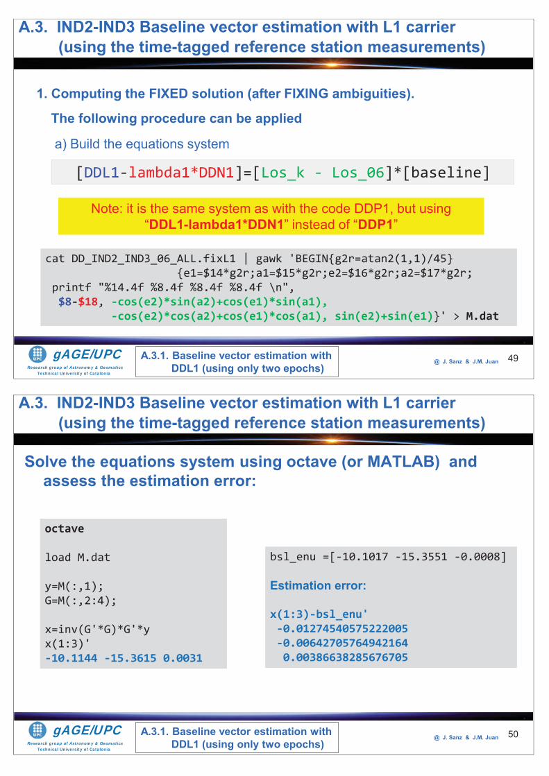
Research group of Astronomy & GeomaticsTechnical University of Catalonia
gAGE/UPC @ J. Sanz & J.M. Juan 49
1. Computing the FIXED solution (after FIXING ambiguities).
The following procedure can be applied
a) Build the equations system
[DDL1-lambda1*DDN1]=[Los_k - Los_06]*[baseline]
Note: it is the same system as with the code DDP1, but using “DDL1-lambda1*DDN1” instead of “DDP1”
cat DD_IND2_IND3_06_ALL.fixL1 | gawk 'BEGIN{g2r=atan2(1,1)/45} {e1=$14*g2r;a1=$15*g2r;e2=$16*g2r;a2=$17*g2r;
printf "%14.4f %8.4f %8.4f %8.4f \n",$8-$18, -cos(e2)*sin(a2)+cos(e1)*sin(a1),
-cos(e2)*cos(a2)+cos(e1)*cos(a1), sin(e2)+sin(e1)}' > M.dat
A.3. IND2-IND3 Baseline vector estimation with L1 carrier(using the time-tagged reference station measurements)
A.3.1. Baseline vector estimation with DDL1 (using only two epochs)
Research group of Astronomy & GeomaticsTechnical University of Catalonia
gAGE/UPC @ J. Sanz & J.M. Juan
Solve the equations system using octave (or MATLAB) and assess the estimation error:
50
octave
load M.dat
y=M(:,1);G=M(:,2:4);
x=inv(G'*G)*G'*yx(1:3)'-10.1144 -15.3615 0.0031
bsl_enu =[-10.1017 -15.3551 -0.0008]
Estimation error:
x(1:3)-bsl_enu'-0.01274540575222005-0.006427057649421640.00386638285676705
A.3. IND2-IND3 Baseline vector estimation with L1 carrier(using the time-tagged reference station measurements)
A.3.1. Baseline vector estimation with DDL1 (using only two epochs)
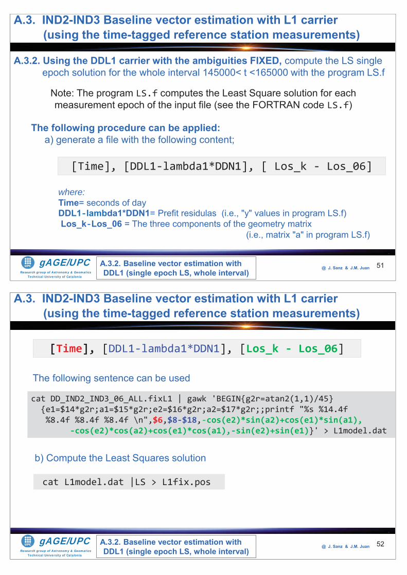
Research group of Astronomy & GeomaticsTechnical University of Catalonia
gAGE/UPC @ J. Sanz & J.M. Juan 51
A.3.2. Using the DDL1 carrier with the ambiguities FIXED, compute the LS single epoch solution for the whole interval 145000< t <165000 with the program LS.f
Note: The program LS.f computes the Least Square solution for eachmeasurement epoch of the input file (see the FORTRAN code LS.f)
The following procedure can be applied:a) generate a file with the following content;
[Time], [DDL1-lambda1*DDN1], [ Los_k - Los_06]
where:Time= seconds of day DDL1-lambda1*DDN1= Prefit residulas (i.e., "y" values in program LS.f)Los_k-Los_06 = The three components of the geometry matrix
(i.e., matrix "a" in program LS.f)
A.3.2. Baseline vector estimation with DDL1 (single epoch LS, whole interval)
A.3. IND2-IND3 Baseline vector estimation with L1 carrier(using the time-tagged reference station measurements)
Research group of Astronomy & GeomaticsTechnical University of Catalonia
gAGE/UPC @ J. Sanz & J.M. Juan 52
The following sentence can be used
cat DD_IND2_IND3_06_ALL.fixL1 | gawk 'BEGIN{g2r=atan2(1,1)/45} {e1=$14*g2r;a1=$15*g2r;e2=$16*g2r;a2=$17*g2r;;printf "%s %14.4f%8.4f %8.4f %8.4f \n",$6,$8-$18,-cos(e2)*sin(a2)+cos(e1)*sin(a1),
-cos(e2)*cos(a2)+cos(e1)*cos(a1),-sin(e2)+sin(e1)}' > L1model.dat
[Time], [DDL1-lambda1*DDN1], [Los_k - Los_06]
b) Compute the Least Squares solution
cat L1model.dat |LS > L1fix.pos
A.3. IND2-IND3 Baseline vector estimation with L1 carrier(using the time-tagged reference station measurements)
A.3.2. Baseline vector estimation with DDL1 (single epoch LS, whole interval)
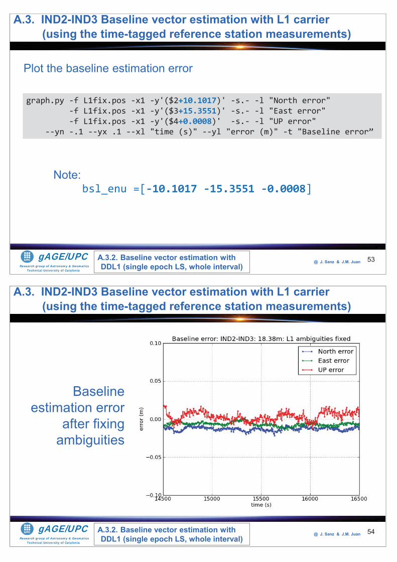
Research group of Astronomy & GeomaticsTechnical University of Catalonia
gAGE/UPC @ J. Sanz & J.M. Juan 53
Plot the baseline estimation error
graph.py -f L1fix.pos -x1 -y'($2+10.1017)' -s.- -l "North error" -f L1fix.pos -x1 -y'($3+15.3551)' -s.- -l "East error" -f L1fix.pos -x1 -y'($4+0.0008)' -s.- -l "UP error"
--yn -.1 --yx .1 --xl "time (s)" --yl "error (m)" -t "Baseline error”
Note:bsl_enu =[-10.1017 -15.3551 -0.0008]
A.3. IND2-IND3 Baseline vector estimation with L1 carrier(using the time-tagged reference station measurements)
A.3.2. Baseline vector estimation with DDL1 (single epoch LS, whole interval)
Research group of Astronomy & GeomaticsTechnical University of Catalonia
gAGE/UPC @ J. Sanz & J.M. Juan 54
Baseline estimation error
after fixing ambiguities
A.3. IND2-IND3 Baseline vector estimation with L1 carrier(using the time-tagged reference station measurements)
A.3.2. Baseline vector estimation with DDL1 (single epoch LS, whole interval)
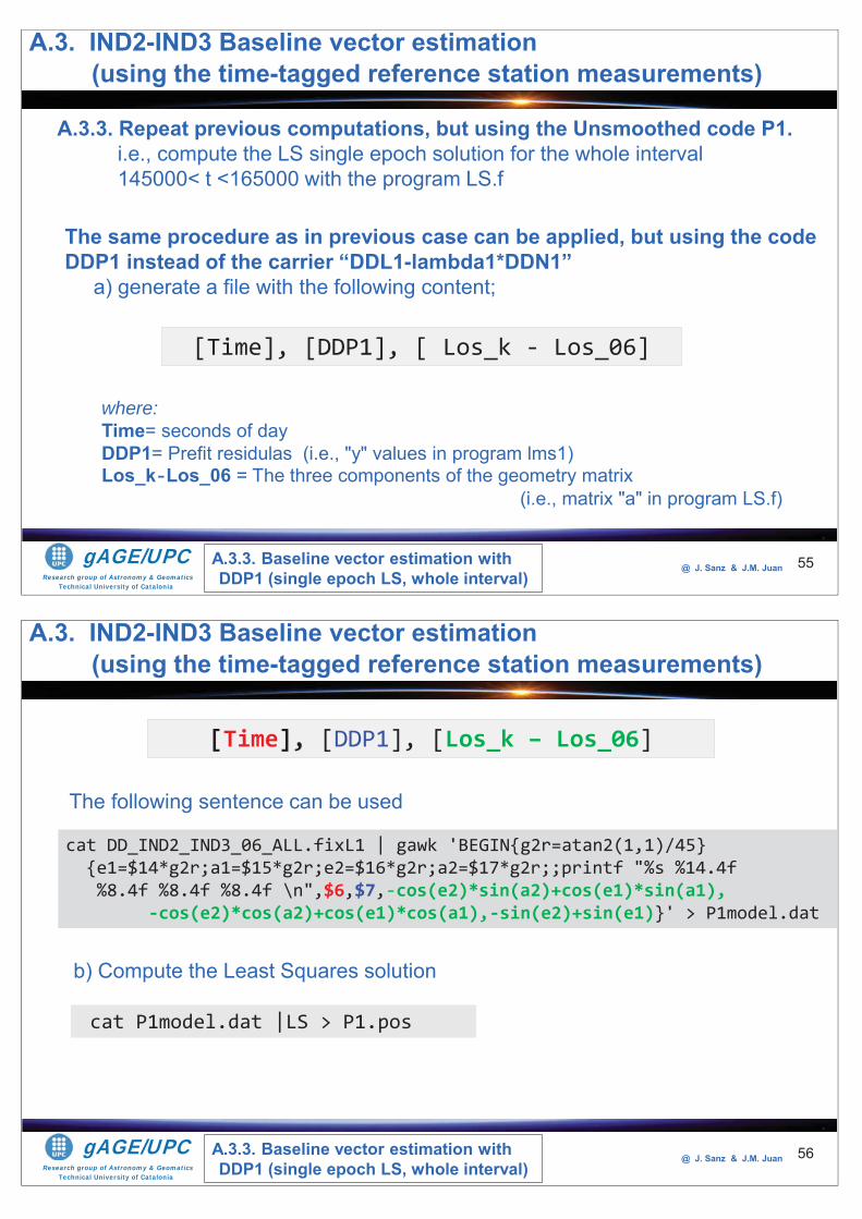
Research group of Astronomy & GeomaticsTechnical University of Catalonia
gAGE/UPC @ J. Sanz & J.M. Juan 55
A.3.3. Repeat previous computations, but using the Unsmoothed code P1. i.e., compute the LS single epoch solution for the whole interval 145000< t <165000 with the program LS.f
The same procedure as in previous case can be applied, but using the code DDP1 instead of the carrier “DDL1-lambda1*DDN1”
a) generate a file with the following content;
[Time], [DDP1], [ Los_k - Los_06]
where:Time= seconds of day DDP1= Prefit residulas (i.e., "y" values in program lms1)Los_k-Los_06 = The three components of the geometry matrix
(i.e., matrix "a" in program LS.f)
A.3. IND2-IND3 Baseline vector estimation (using the time-tagged reference station measurements)
A.3.3. Baseline vector estimation with DDP1 (single epoch LS, whole interval)
Research group of Astronomy & GeomaticsTechnical University of Catalonia
gAGE/UPC @ J. Sanz & J.M. Juan 56
The following sentence can be used
cat DD_IND2_IND3_06_ALL.fixL1 | gawk 'BEGIN{g2r=atan2(1,1)/45} {e1=$14*g2r;a1=$15*g2r;e2=$16*g2r;a2=$17*g2r;;printf "%s %14.4f%8.4f %8.4f %8.4f \n",$6,$7,-cos(e2)*sin(a2)+cos(e1)*sin(a1),
-cos(e2)*cos(a2)+cos(e1)*cos(a1),-sin(e2)+sin(e1)}' > P1model.dat
[Time], [DDP1], [Los_k – Los_06]
b) Compute the Least Squares solution
cat P1model.dat |LS > P1.pos
A.3. IND2-IND3 Baseline vector estimation (using the time-tagged reference station measurements)
A.3.3. Baseline vector estimation with DDP1 (single epoch LS, whole interval)
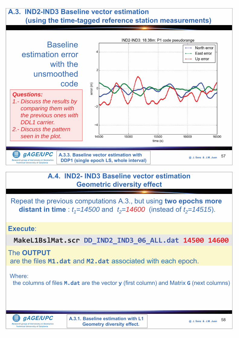
Research group of Astronomy & GeomaticsTechnical University of Catalonia
gAGE/UPC @ J. Sanz & J.M. Juan 57
Baseline estimation error
with the unsmoothed
code Questions: 1.- Discuss the results by
comparing them with the previous ones with DDL1 carrier.
2.- Discuss the pattern seen in the plot.
A.3. IND2-IND3 Baseline vector estimation (using the time-tagged reference station measurements)
A.3.3. Baseline vector estimation with DDP1 (single epoch LS, whole interval)
Research group of Astronomy & GeomaticsTechnical University of Catalonia
gAGE/UPC @ J. Sanz & J.M. Juan
Repeat the previous computations A.3., but using two epochs more distant in time : t1=14500 and t2=14600 (instead of t2=14515).
58
A.4. IND2- IND3 Baseline vector estimation Geometric diversity effect
The OUTPUTare the files M1.dat and M2.dat associated with each epoch.
MakeL1BslMat.scr DD_IND2_IND3_06_ALL.dat 14500 14600Execute:
Where: the columns of files M.dat are the vector y (first column) and Matrix G (next columns)
A.3.1. Baseline estimation with L1 Geometry diversity effect.
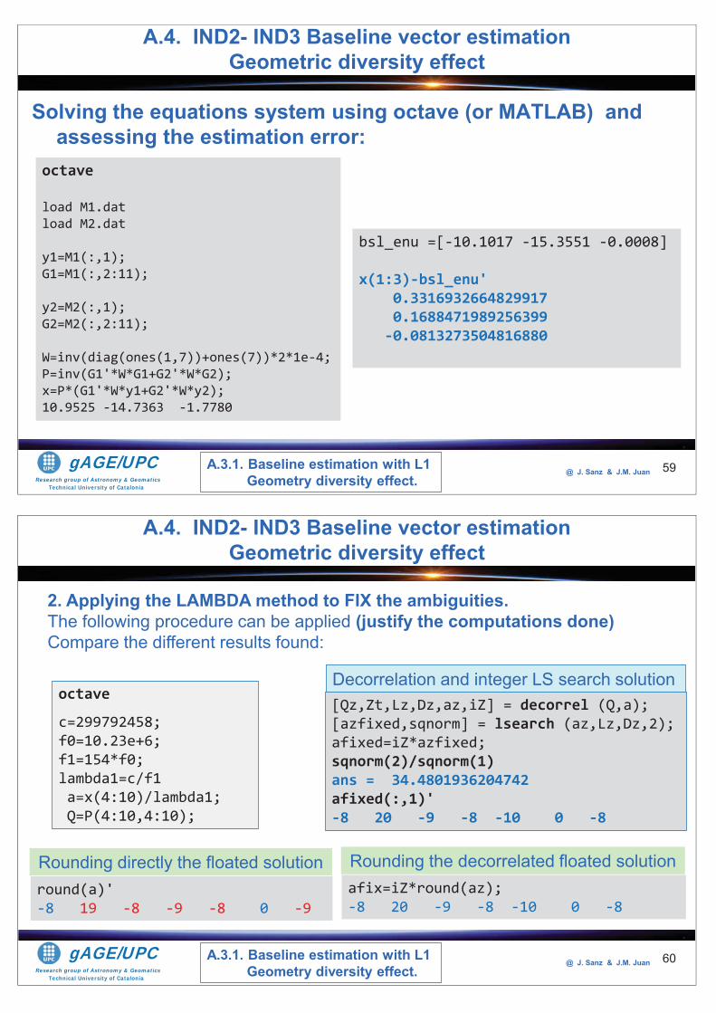
Research group of Astronomy & GeomaticsTechnical University of Catalonia
gAGE/UPC @ J. Sanz & J.M. Juan
Solving the equations system using octave (or MATLAB) and assessing the estimation error:
59
octave
load M1.datload M2.dat
y1=M1(:,1);G1=M1(:,2:11);
y2=M2(:,1);G2=M2(:,2:11);
W=inv(diag(ones(1,7))+ones(7))*2*1e-4;P=inv(G1'*W*G1+G2'*W*G2);x=P*(G1'*W*y1+G2'*W*y2);10.9525 -14.7363 -1.7780
bsl_enu =[-10.1017 -15.3551 -0.0008]
x(1:3)-bsl_enu'0.33169326648299170.1688471989256399-0.0813273504816880
A.3.1. Baseline estimation with L1 Geometry diversity effect.
A.4. IND2- IND3 Baseline vector estimation Geometric diversity effect
Research group of Astronomy & GeomaticsTechnical University of Catalonia
gAGE/UPC @ J. Sanz & J.M. Juan 60
octave
c=299792458;f0=10.23e+6;f1=154*f0;lambda1=c/f1a=x(4:10)/lambda1;Q=P(4:10,4:10);
afix=iZ*round(az);-8 20 -9 -8 -10 0 -8
[Qz,Zt,Lz,Dz,az,iZ] = decorrel (Q,a);[azfixed,sqnorm] = lsearch (az,Lz,Dz,2);afixed=iZ*azfixed;sqnorm(2)/sqnorm(1)ans = 34.4801936204742afixed(:,1)'-8 20 -9 -8 -10 0 -8
Rounding the decorrelated floated solutionround(a)'-8 19 -8 -9 -8 0 -9
Rounding directly the floated solution
Decorrelation and integer LS search solution
A.3.1. Baseline estimation with L1 Geometry diversity effect.
A.4. IND2- IND3 Baseline vector estimation Geometric diversity effect
2. Applying the LAMBDA method to FIX the ambiguities. The following procedure can be applied (justify the computations done)Compare the different results found:
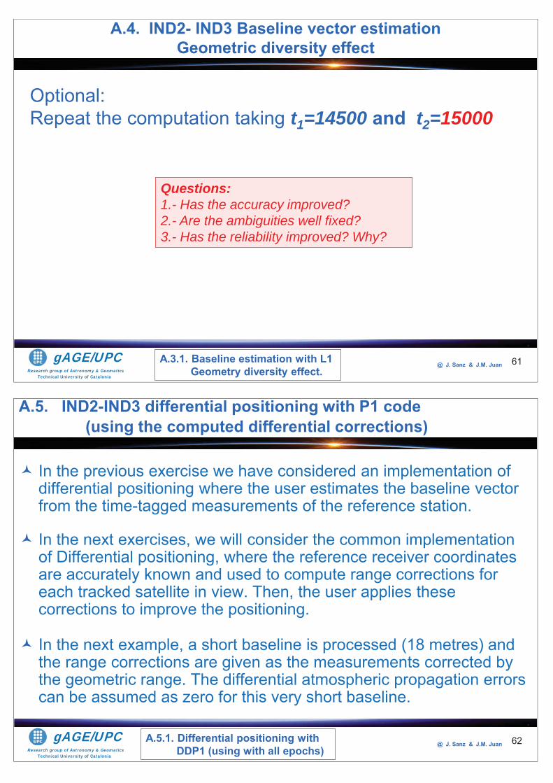
Research group of Astronomy & GeomaticsTechnical University of Catalonia
gAGE/UPC @ J. Sanz & J.M. Juan 61
Optional:Repeat the computation taking t1=14500 and t2=15000
Questions: 1.- Has the accuracy improved?2.- Are the ambiguities well fixed?3.- Has the reliability improved? Why?
A.3.1. Baseline estimation with L1 Geometry diversity effect.
A.4. IND2- IND3 Baseline vector estimation Geometric diversity effect
Research group of Astronomy & GeomaticsTechnical University of Catalonia
gAGE/UPC @ J. Sanz & J.M. Juan 62
In the previous exercise we have considered an implementation of differential positioning where the user estimates the baseline vector from the time-tagged measurements of the reference station.
In the next exercises, we will consider the common implementation of Differential positioning, where the reference receiver coordinates are accurately known and used to compute range corrections for each tracked satellite in view. Then, the user applies these corrections to improve the positioning.
In the next example, a short baseline is processed (18 metres) and the range corrections are given as the measurements corrected by the geometric range. The differential atmospheric propagation errors can be assumed as zero for this very short baseline.
A.5. IND2-IND3 differential positioning with P1 code(using the computed differential corrections)
A.5.1. Differential positioning with DDP1 (using with all epochs)
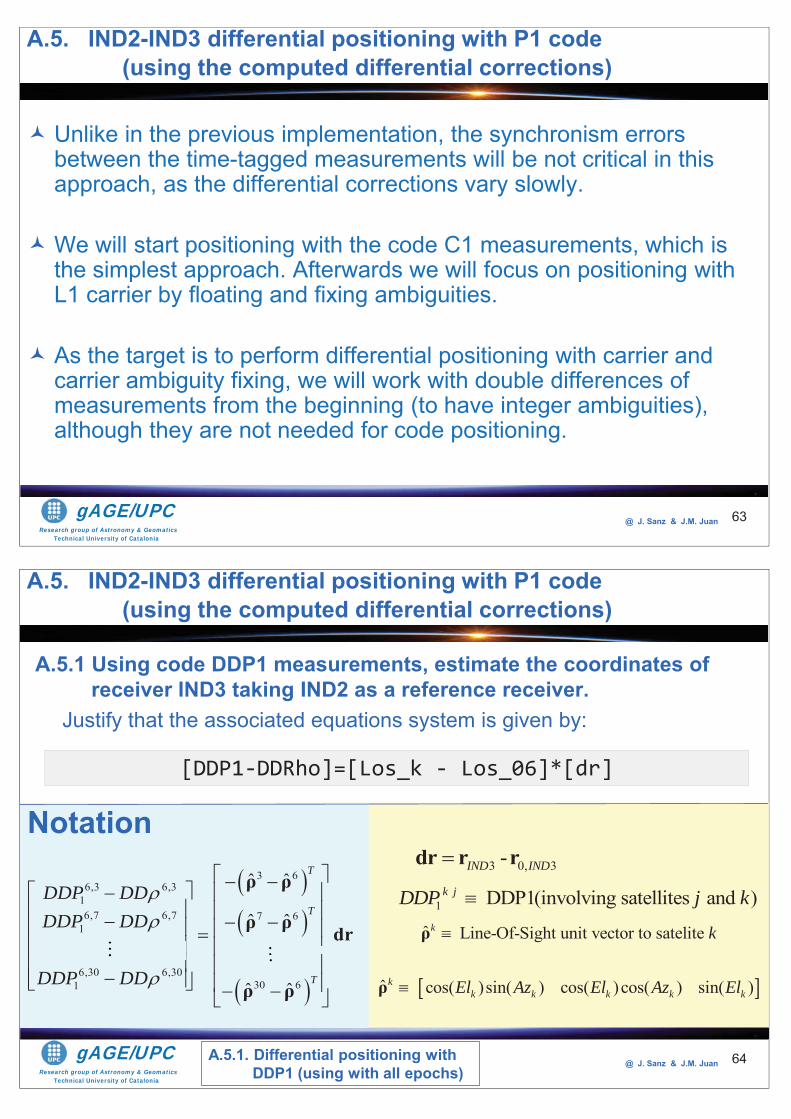
Research group of Astronomy & GeomaticsTechnical University of Catalonia
gAGE/UPC @ J. Sanz & J.M. Juan 63
Unlike in the previous implementation, the synchronism errors between the time-tagged measurements will be not critical in this approach, as the differential corrections vary slowly.
We will start positioning with the code C1 measurements, which is the simplest approach. Afterwards we will focus on positioning with L1 carrier by floating and fixing ambiguities.
As the target is to perform differential positioning with carrier and carrier ambiguity fixing, we will work with double differences of measurements from the beginning (to have integer ambiguities), although they are not needed for code positioning.
A.5. IND2-IND3 differential positioning with P1 code(using the computed differential corrections)
Research group of Astronomy & GeomaticsTechnical University of Catalonia
gAGE/UPC @ J. Sanz & J.M. Juan
A.5.1 Using code DDP1 measurements, estimate the coordinates of receiver IND3 taking IND2 as a reference receiver.
Justify that the associated equations system is given by:
64
[DDP1-DDRho]=[Los_k - Los_06]*[dr]
3 66,3 6,3
16,7 6,7 7 6
1
6,30 6,3030 61
ˆ ˆ
ˆ ˆ
ˆ ˆ
T
T
T
DDP DDDDP DD
DDP DD
ρ ρ
ρ ρ dr
ρ ρ
1 DDP1(involving satellites and )k jDDP j kˆ Line-Of-Sight unit vector to satelite k kρ
ˆ cos( )sin( ) cos( )cos( ) sin( )kk k k k kEl Az El Az Elρ
3 0, 3-IND INDdr r rNotation
A.5.1. Differential positioning with DDP1 (using with all epochs)
A.5. IND2-IND3 differential positioning with P1 code(using the computed differential corrections)
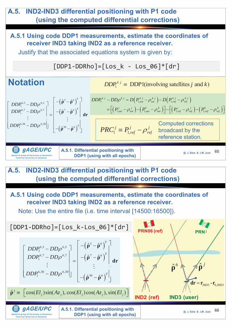
Research group of Astronomy & GeomaticsTechnical University of Catalonia
gAGE/UPC @ J. Sanz & J.M. Juan
A.5.1 Using code DDP1 measurements, estimate the coordinates of receiver IND3 taking IND2 as a reference receiver.
Justify that the associated equations system is given by:
65
[DDP1-DDRho]=[Los_k - Los_06]*[dr]
A.5.1. Differential positioning with DDP1 (using with all epochs)
A.5. IND2-IND3 differential positioning with P1 code(using the computed differential corrections)
Notation
1 1,j j j
ref refPRC PComputed corrections broadcast by the reference station.
3 66,3 6,3
16,7 6,7 7 6
1
6,30 6,3030 61
ˆ ˆ
ˆ ˆ
ˆ ˆ
T
T
T
DDP DDDDP DD
DDP DD
ρ ρ
ρ ρ dr
ρ ρ
1 1, 1,
1, 1, 1, 1,
k j k j k j k j k j k jusr usr ref ref
j j k k j j k kusr usr usr usr ref ref ref ref
DDP DD D P D P
P P P P
1 DDP1(involving satellites and )k jDDP j k
Research group of Astronomy & GeomaticsTechnical University of Catalonia
gAGE/UPC @ J. Sanz & J.M. Juan
IND3 (user)IND2 (ref)
PRN06 (ref) PRN j
A.5.1 Using code DDP1 measurements, estimate the coordinates of receiver IND3 taking IND2 as a reference receiver.
Note: Use the entire file (i.e. time interval [14500:16500]).
66
[DDP1-DDRho]=[Los_k-Los_06]*[dr]
6ρ ˆ jρ
3 66,3 6,3
16,7 6,7 7 6
1
6,30 6,3030 61
ˆ ˆ
ˆ ˆ
ˆ ˆ
T
T
T
DDP DDDDP DD
DDP DD
ρ ρ
ρ ρ dr
ρ ρ
A.5.1. Differential positioning with DDP1 (using with all epochs)
A.5. IND2-IND3 differential positioning with P1 code(using the computed differential corrections)
3 0, 3-IND INDdr r rˆ cos( )sin( ), cos( )cos( ), sin( )j
j j j j jEl Az El Az Elρ
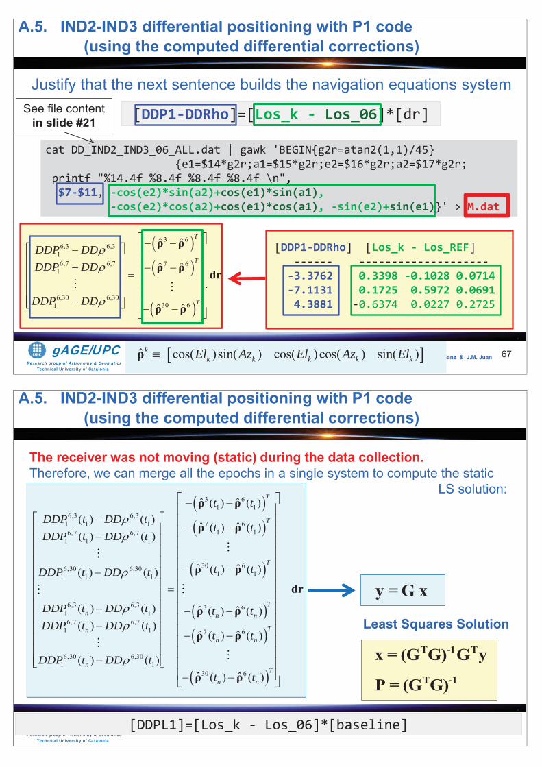
Research group of Astronomy & GeomaticsTechnical University of Catalonia
gAGE/UPC @ J. Sanz & J.M. Juan 67
cat DD_IND2_IND3_06_ALL.dat | gawk 'BEGIN{g2r=atan2(1,1)/45} {e1=$14*g2r;a1=$15*g2r;e2=$16*g2r;a2=$17*g2r;
printf "%14.4f %8.4f %8.4f %8.4f \n",$7-$11, -cos(e2)*sin(a2)+cos(e1)*sin(a1),
-cos(e2)*cos(a2)+cos(e1)*cos(a1), -sin(e2)+sin(e1)}' > M.dat
Justify that the next sentence builds the navigation equations system
[DDP1-DDRho]=[Los_k - Los_06]*[dr]
[DDP1-DDRho] [Los_k - Los_REF] ------ ---------------------3.3762 0.3398 -0.1028 0.0714-7.1131 0.1725 0.5972 0.0691 4.3881 -0.6374 0.0227 0.2725
ˆ cos( )sin( ) cos( )cos( ) sin( )kk k k k kEl Az El Az Elρ
3 66,3 6,3
16,7 6,7 7 6
1
6,30 6,3030 61
ˆ ˆ
ˆ ˆ
ˆ ˆ
T
T
T
DDP DDDDP DD
DDP DD
ρ ρ
ρ ρ dr
ρ ρ
A.5. IND2-IND3 differential positioning with P1 code(using the computed differential corrections)
See file content in slide #21
Research group of Astronomy & GeomaticsTechnical University of Catalonia
gAGE/UPC @ J. Sanz & J.M. Juan 68[DDPL1]=[Los_k - Los_06]*[baseline]
3 61 1
6,3 6,31 1 1 7 6
16,7 6,71 1 1
6,30 6,301 1 1
6,3 6,31 16,7 6,7
1 1
6,30 6,301 1
ˆ ˆ( ) ( )( ) ( ) ˆ ˆ( ) (( ) ( )
( ) ( )
( ) ( )( ) ( )
( ) ( )
T
n
n
n
t tDDP t DD t
tDDP t DD t
DDP t DD t
DDP t DD tDDP t DD t
DDP t DD t
ρ ρ
ρ ρ 1
30 61 1
3 6
7 6
30 6
)
ˆ ˆ( ) ( )
ˆ ˆ( ) ( )
ˆ ˆ( ) ( )
ˆ ˆ( ) ( )
T
T
T
n n
T
n n
T
n n
t
t t
t t
t t
t t
ρ ρdr
ρ ρ
ρ ρ
ρ ρ
The receiver was not moving (static) during the data collection. Therefore, we can merge all the epochs in a single system to compute the static
LS solution:
y =G x
T -1 Tx = (G G) G yT -1P = (G G)
Least Squares Solution
A.5. IND2-IND3 differential positioning with P1 code(using the computed differential corrections)
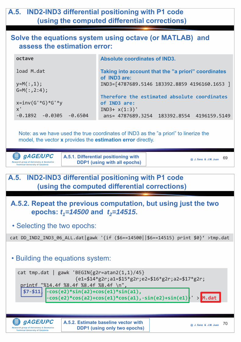
Research group of Astronomy & GeomaticsTechnical University of Catalonia
gAGE/UPC @ J. Sanz & J.M. Juan
Solve the equations system using octave (or MATLAB) and assess the estimation error:
69
octave
load M.dat
y=M(:,1);G=M(:,2:4);
x=inv(G'*G)*G'*yx'-0.1892 -0.0305 -0.6504
Absolute coordinates of IND3.
Taking into account that the ”a priori” coordinates of IND3 are: IND3=[4787689.5146 183392.8859 4196160.1653 ]
Therefore the estimated absolute coordinates of IND3 are:IND3+ x(1:3)'ans= 4787689.3254 183392.8554 4196159.5149
A.5.1. Differential positioning with DDP1 (using with all epochs)
Note: as we have used the true coordinates of IND3 as the ”a priori” to linerize the model, the vector x provides the estimation error directly.
A.5. IND2-IND3 differential positioning with P1 code(using the computed differential corrections)
Research group of Astronomy & GeomaticsTechnical University of Catalonia
gAGE/UPC @ J. Sanz & J.M. Juan
A.5.2. Repeat the previous computation, but using just the two epochs: t1=14500 and t2=14515.
70
cat DD_IND2_IND3_06_ALL.dat|gawk '{if ($6==14500||$6==14515) print $0}‘ >tmp.dat
• Selecting the two epochs:
• Building the equations system:
A.5.2. Estimate baseline vector with DDP1 (using only two epochs)
cat tmp.dat | gawk 'BEGIN{g2r=atan2(1,1)/45} {e1=$14*g2r;a1=$15*g2r;e2=$16*g2r;a2=$17*g2r;
printf "%14.4f %8.4f %8.4f %8.4f \n",$7-$11, -cos(e2)*sin(a2)+cos(e1)*sin(a1),
-cos(e2)*cos(a2)+cos(e1)*cos(a1),-sin(e2)+sin(e1)}' > M.dat
A.5. IND2-IND3 differential positioning with P1 code(using the computed differential corrections)
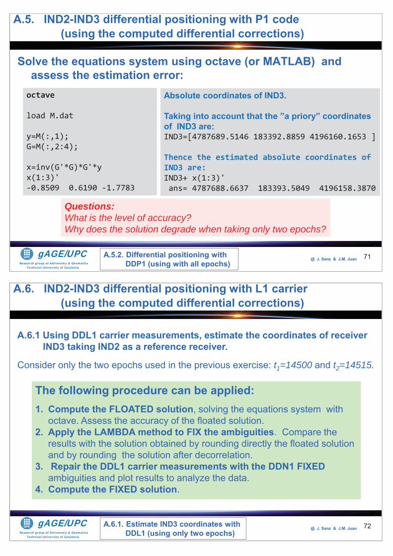
Research group of Astronomy & GeomaticsTechnical University of Catalonia
gAGE/UPC @ J. Sanz & J.M. Juan
Solve the equations system using octave (or MATLAB) and assess the estimation error:
71
octave
load M.dat
y=M(:,1);G=M(:,2:4);
x=inv(G'*G)*G'*yx(1:3)'-0.8509 0.6190 -1.7783
Absolute coordinates of IND3.
Taking into account that the ”a priory” coordinates of IND3 are: IND3=[4787689.5146 183392.8859 4196160.1653 ]
Thence the estimated absolute coordinates of IND3 are:IND3+ x(1:3)'ans= 4787688.6637 183393.5049 4196158.3870
A.5.2. Differential positioning with DDP1 (using with all epochs)
Questions:What is the level of accuracy?Why does the solution degrade when taking only two epochs?
A.5. IND2-IND3 differential positioning with P1 code(using the computed differential corrections)
Research group of Astronomy & GeomaticsTechnical University of Catalonia
gAGE/UPC @ J. Sanz & J.M. Juan 72
A.6.1 Using DDL1 carrier measurements, estimate the coordinates of receiver IND3 taking IND2 as a reference receiver.
Consider only the two epochs used in the previous exercise: t1=14500 and t2=14515.
The following procedure can be applied:1. Compute the FLOATED solution, solving the equations system with
octave. Assess the accuracy of the floated solution.2. Apply the LAMBDA method to FIX the ambiguities. Compare the
results with the solution obtained by rounding directly the floated solution and by rounding the solution after decorrelation.
3. Repair the DDL1 carrier measurements with the DDN1 FIXED ambiguities and plot results to analyze the data.
4. Compute the FIXED solution.
A.6.1. Estimate IND3 coordinates with DDL1 (using only two epochs)
A.6. IND2-IND3 differential positioning with L1 carrier(using the computed differential corrections)
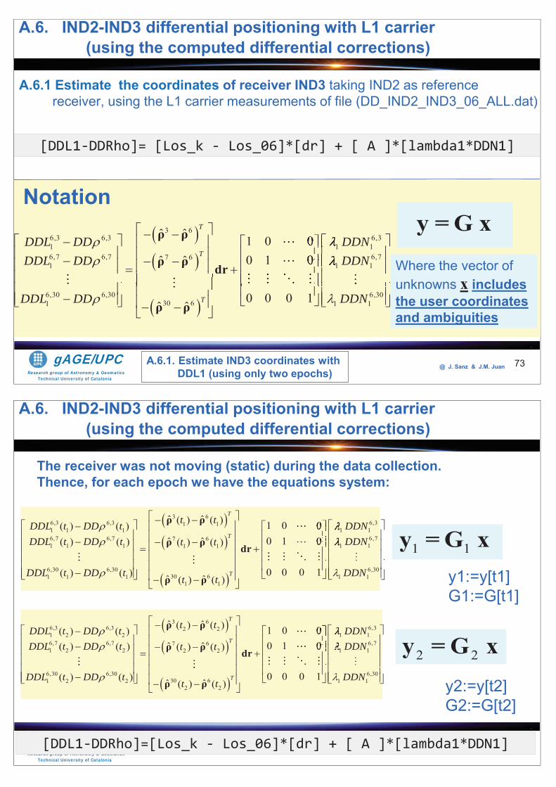
Research group of Astronomy & GeomaticsTechnical University of Catalonia
gAGE/UPC @ J. Sanz & J.M. Juan
A.6.1 Estimate the coordinates of receiver IND3 taking IND2 as reference receiver, using the L1 carrier measurements of file (DD_IND2_IND3_06_ALL.dat)
73
[DDL1-DDRho]= [Los_k - Los_06]*[dr] + [ A ]*[lambda1*DDN1]
3 66,3 6,3 6,31 1 16,7 6,7 6,77 61 1 1
6,30 6,30 6,3030 61 1 1
ˆ ˆ 1 0 00 1 0ˆ ˆ
0 0 0 1ˆ ˆ
T
T
T
DDL DD DDNDDL DD DDN
DDL DD DDN
ρ ρ
ρ ρ dr
ρ ρ
00
Notation
Where the vector of unknowns x includes the user coordinates and ambiguities
y =G x
A.6.1. Estimate IND3 coordinates with DDL1 (using only two epochs)
A.6. IND2-IND3 differential positioning with L1 carrier(using the computed differential corrections)
Research group of Astronomy & GeomaticsTechnical University of Catalonia
gAGE/UPC @ J. Sanz & J.M. Juan 74[DDL1-DDRho]=[Los_k - Los_06]*[dr] + [ A ]*[lambda1*DDN1]
3 66,3 6,3 6,31 11 1 1 1 16,7 6,7 67 61 1 1 1 11 1
6,30 6,3030 61 1 1
1 1
ˆ ˆ( ) ( ) 1 0 0( ) ( )0 1 0ˆ ˆ( ) ( ) ( ) ( )
0 0 0 1( ) ( ) ˆ ˆ( ) ( )
T
T
T
t tDDL t DD t DDNDDL t DD t DDNt t
DDL t DD tt t
ρ ρ
ρ ρ dr
ρ ρ
00 ,7
6,301 1DDN
3 66,3 6,3 6,32 21 2 2 1 16,7 6,7 67 61 2 2 1 12 2
6,30 6,3030 61 2 2
2 2
ˆ ˆ( ) ( ) 1 0 0( ) ( )0 1 0ˆ ˆ( ) ( ) ( ) ( )
0 0 0 1( ) ( ) ˆ ˆ( ) ( )
T
T
T
t tDDL t DD t DDNDDL t DD t DDNt t
DDL t DD tt t
ρ ρ
ρ ρ dr
ρ ρ
00 ,7
6,301 1DDN
1 1y =G xy1:=y[t1] G1:=G[t1]
2 2y = G xy2:=y[t2] G2:=G[t2]
The receiver was not moving (static) during the data collection. Thence, for each epoch we have the equations system:
A.6. IND2-IND3 differential positioning with L1 carrier(using the computed differential corrections)
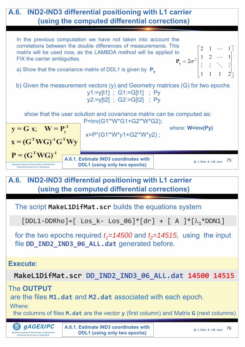
Research group of Astronomy & GeomaticsTechnical University of Catalonia
gAGE/UPC @ J. Sanz & J.M. Juan 75
In the previous computation we have not taken into account thecorrelations between the double differences of measurements. Thismatrix will be used now, as the LAMBDA method will be applied toFIX the carrier ambiguities.
a) Show that the covariance matrix of DDL1 is given by Py
2
2 1 11 2 1
2
1 1 1 2
1111
yP
b) Given the measurement vectors (y) and Geometry matrices (G) for two epochsy1:=y[t1] ; G1:=G[t1] ; Pyy2:=y[t2] ; G2:=G[t2] ; Py
show that the user solution and covariance matrix can be computed as:P=inv(G1'*W*G1+G2'*W*G2);
where: W=inv(Py)x=P*(G1'*W*y1+G2'*W*y2) ;
; -1yy = G x W = P
T -1 Tx = (G WG) G WyT -1P = (G WG) A.6.1. Estimate IND3 coordinates with
DDL1 (using only two epochs)
A.6. IND2-IND3 differential positioning with L1 carrier(using the computed differential corrections)
Research group of Astronomy & GeomaticsTechnical University of Catalonia
gAGE/UPC @ J. Sanz & J.M. Juan 76
The script MakeL1DifMat.scr builds the equations system
The OUTPUTare the files M1.dat and M2.dat associated with each epoch.
for the two epochs required t1=14500 and t2=14515, using the input file DD_IND2_IND3_06_ALL.dat generated before.
[DDL1-DDRho]=[ Los_k- Los_06]*[dr] + [ A ]*[ 1*DDN1]
MakeL1DifMat.scr DD_IND2_IND3_06_ALL.dat 14500 14515Execute:
Where: the columns of files M.dat are the vector y (first column) and Matrix G (next columns)
A.6.1. Estimate IND3 coordinates with DDL1 (using only two epochs)
A.6. IND2-IND3 differential positioning with L1 carrier(using the computed differential corrections)
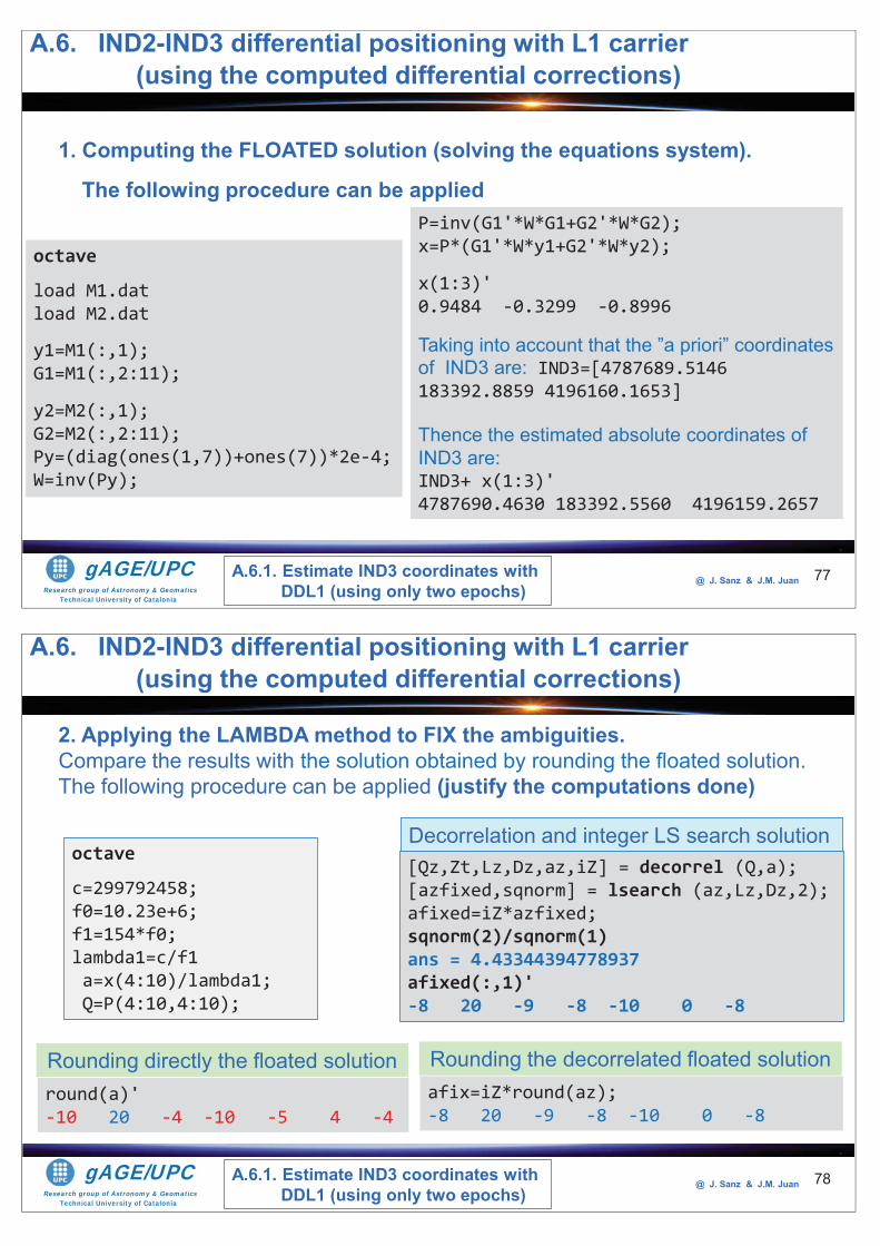
Research group of Astronomy & GeomaticsTechnical University of Catalonia
gAGE/UPC @ J. Sanz & J.M. Juan 77
1. Computing the FLOATED solution (solving the equations system).
The following procedure can be applied
octave
load M1.datload M2.dat
y1=M1(:,1);G1=M1(:,2:11);
y2=M2(:,1);G2=M2(:,2:11);Py=(diag(ones(1,7))+ones(7))*2e-4;W=inv(Py);
P=inv(G1'*W*G1+G2'*W*G2);x=P*(G1'*W*y1+G2'*W*y2);
x(1:3)'0.9484 -0.3299 -0.8996
Taking into account that the ”a priori” coordinates of IND3 are: IND3=[4787689.5146 183392.8859 4196160.1653]
Thence the estimated absolute coordinates of IND3 are:IND3+ x(1:3)'4787690.4630 183392.5560 4196159.2657
A.6.1. Estimate IND3 coordinates with DDL1 (using only two epochs)
A.6. IND2-IND3 differential positioning with L1 carrier(using the computed differential corrections)
Research group of Astronomy & GeomaticsTechnical University of Catalonia
gAGE/UPC @ J. Sanz & J.M. Juan 78
2. Applying the LAMBDA method to FIX the ambiguities. Compare the results with the solution obtained by rounding the floated solution. The following procedure can be applied (justify the computations done)
octave
c=299792458;f0=10.23e+6;f1=154*f0;lambda1=c/f1a=x(4:10)/lambda1;Q=P(4:10,4:10);
afix=iZ*round(az);-8 20 -9 -8 -10 0 -8
[Qz,Zt,Lz,Dz,az,iZ] = decorrel (Q,a);[azfixed,sqnorm] = lsearch (az,Lz,Dz,2);afixed=iZ*azfixed;sqnorm(2)/sqnorm(1)ans = 4.43344394778937afixed(:,1)'-8 20 -9 -8 -10 0 -8
Rounding the decorrelated floated solutionround(a)'-10 20 -4 -10 -5 4 -4
Rounding directly the floated solution
Decorrelation and integer LS search solution
A.6.1. Estimate IND3 coordinates with DDL1 (using only two epochs)
A.6. IND2-IND3 differential positioning with L1 carrier(using the computed differential corrections)
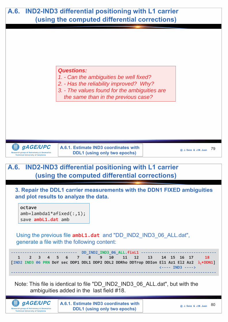
Research group of Astronomy & GeomaticsTechnical University of Catalonia
gAGE/UPC @ J. Sanz & J.M. Juan 79
Questions: 1. - Can the ambiguities be well fixed?2. - Has the reliability improved? Why?3. - The values found for the ambiguities are
the same than in the previous case?
A.6.1. Estimate IND3 coordinates with DDL1 (using only two epochs)
A.6. IND2-IND3 differential positioning with L1 carrier(using the computed differential corrections)
Research group of Astronomy & GeomaticsTechnical University of Catalonia
gAGE/UPC @ J. Sanz & J.M. Juan 80
3. Repair the DDL1 carrier measurements with the DDN1 FIXED ambiguities and plot results to analyze the data.
octaveamb=lambda1*afixed(:,1);save ambL1.dat amb
Using the previous file ambL1.dat and "DD_IND2_IND3_06_ALL.dat",generate a file with the following content:
----------------------------- DD_IND2_IND3_06_ALL.fixL1 ---------------------------------1 2 3 4 5 6 7 8 9 10 11 12 13 14 15 16 17 18
[IND2 IND3 06 PRN DoY sec DDP1 DDL1 DDP2 DDL2 DDRho DDTrop DDIon El1 Az1 El2 Az2 DDN1]<---- IND3 ---->
------------------------------------------------------------------------------------------
Note: This file is identical to file "DD_IND2_IND3_06_ALL.dat", but with the ambiguities added in the last field #18.
A.6.1. Estimate IND3 coordinates with DDL1 (using only two epochs)
A.6. IND2-IND3 differential positioning with L1 carrier(using the computed differential corrections)
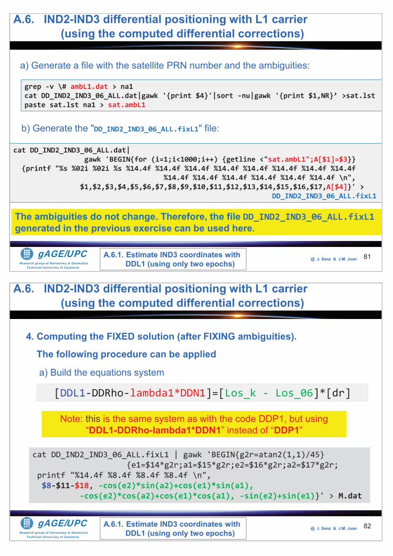
Research group of Astronomy & GeomaticsTechnical University of Catalonia
gAGE/UPC @ J. Sanz & J.M. Juan 81
grep -v \# ambL1.dat > na1cat DD_IND2_IND3_06_ALL.dat|gawk '{print $4}'|sort -nu|gawk '{print $1,NR}’ >sat.lstpaste sat.lst na1 > sat.ambL1
a) Generate a file with the satellite PRN number and the ambiguities:
cat DD_IND2_IND3_06_ALL.dat|gawk 'BEGIN{for (i=1;i<1000;i++) {getline <"sat.ambL1";A[$1]=$3}}
{printf "%s %02i %02i %s %14.4f %14.4f %14.4f %14.4f %14.4f %14.4f %14.4f %14.4f %14.4f %14.4f %14.4f %14.4f %14.4f %14.4f \n",
$1,$2,$3,$4,$5,$6,$7,$8,$9,$10,$11,$12,$13,$14,$15,$16,$17,A[$4]}' > DD_IND2_IND3_06_ALL.fixL1
b) Generate the "DD_IND2_IND3_06_ALL.fixL1" file:
A.6.1. Estimate IND3 coordinates with DDL1 (using only two epochs)
The ambiguities do not change. Therefore, the file DD_IND2_IND3_06_ALL.fixL1generated in the previous exercise can be used here.
A.6. IND2-IND3 differential positioning with L1 carrier(using the computed differential corrections)
Research group of Astronomy & GeomaticsTechnical University of Catalonia
gAGE/UPC @ J. Sanz & J.M. Juan 82
4. Computing the FIXED solution (after FIXING ambiguities).
The following procedure can be applied
a) Build the equations system
[DDL1-DDRho-lambda1*DDN1]=[Los_k - Los_06]*[dr]
Note: this is the same system as with the code DDP1, but using “DDL1-DDRho-lambda1*DDN1” instead of “DDP1”
cat DD_IND2_IND3_06_ALL.fixL1 | gawk 'BEGIN{g2r=atan2(1,1)/45} {e1=$14*g2r;a1=$15*g2r;e2=$16*g2r;a2=$17*g2r;
printf "%14.4f %8.4f %8.4f %8.4f \n",$8-$11-$18, -cos(e2)*sin(a2)+cos(e1)*sin(a1),
-cos(e2)*cos(a2)+cos(e1)*cos(a1), -sin(e2)+sin(e1)}' > M.dat
A.6.1. Estimate IND3 coordinates with DDL1 (using only two epochs)
A.6. IND2-IND3 differential positioning with L1 carrier(using the computed differential corrections)
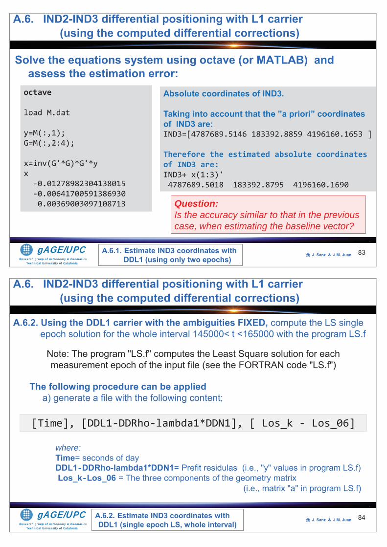
Research group of Astronomy & GeomaticsTechnical University of Catalonia
gAGE/UPC @ J. Sanz & J.M. Juan
Solve the equations system using octave (or MATLAB) and assess the estimation error:
83
octave
load M.dat
y=M(:,1);G=M(:,2:4);
x=inv(G'*G)*G'*yx-0.01278982304138015-0.006417005913869300.00369003097108713
Absolute coordinates of IND3.
Taking into account that the ”a priori” coordinates of IND3 are: IND3=[4787689.5146 183392.8859 4196160.1653 ]
Therefore the estimated absolute coordinates of IND3 are:IND3+ x(1:3)'4787689.5018 183392.8795 4196160.1690
A.6.1. Estimate IND3 coordinates with DDL1 (using only two epochs)
Question: Is the accuracy similar to that in the previous case, when estimating the baseline vector?
A.6. IND2-IND3 differential positioning with L1 carrier(using the computed differential corrections)
Research group of Astronomy & GeomaticsTechnical University of Catalonia
gAGE/UPC @ J. Sanz & J.M. Juan 84
A.6.2. Using the DDL1 carrier with the ambiguities FIXED, compute the LS single epoch solution for the whole interval 145000< t <165000 with the program LS.f
Note: The program "LS.f" computes the Least Square solution for eachmeasurement epoch of the input file (see the FORTRAN code "LS.f")
The following procedure can be applieda) generate a file with the following content;
[Time], [DDL1-DDRho-lambda1*DDN1], [ Los_k - Los_06]
where:Time= seconds of day DDL1-DDRho-lambda1*DDN1= Prefit residulas (i.e., "y" values in program LS.f)Los_k-Los_06 = The three components of the geometry matrix
(i.e., matrix "a" in program LS.f)
A.6.2. Estimate IND3 coordinates with DDL1 (single epoch LS, whole interval)
A.6. IND2-IND3 differential positioning with L1 carrier(using the computed differential corrections)

Research group of Astronomy & GeomaticsTechnical University of Catalonia
gAGE/UPC @ J. Sanz & J.M. Juan 85
The following sentence can be used
cat DD_IND2_IND3_06_ALL.fixL1 | gawk 'BEGIN{g2r=atan2(1,1)/45} {e1=$14*g2r;a1=$15*g2r;e2=$16*g2r;a2=$17*g2r;;printf "%s %14.4f%8.4f %8.4f %8.4f \n",$6,$8-$11-$18,-cos(e2)*sin(a2)+cos(e1)*sin(a1),
-cos(e2)*cos(a2)+cos(e1)*cos(a1),-sin(e2)+sin(e1)}' > L1model.dat
[Time], [DDL1-DDRho-lambda1*DDN1], [Los_k - Los_06]
b) Compute the Least Squares solution
cat L1model.dat |LS > L1fix.pos
A.6.2. Estimate IND3 coordinates with DDL1 (single epoch LS, whole interval)
A.6. IND2-IND3 differential positioning with L1 carrier(using the computed differential corrections)
Research group of Astronomy & GeomaticsTechnical University of Catalonia
gAGE/UPC @ J. Sanz & J.M. Juan 86
Plot the baseline estimation error
graph.py -f L1fix.pos -x1 –y2 -s.- -l "North error" -f L1fix.pos -x1 –y3 -s.- -l "East error" -f L1fix.pos -x1 –y4 -s.- -l "UP error"
--yn -.1 --yx .1 --xl "time (s)" --yl "error (m)" -t “IND2-IND3: 18.38m: L1 ambiguities fixed”
A.6.2. Estimate IND3 coordinates with DDL1 (single epoch LS, whole interval)
A.6. IND2-IND3 differential positioning with L1 carrier(using the computed differential corrections)
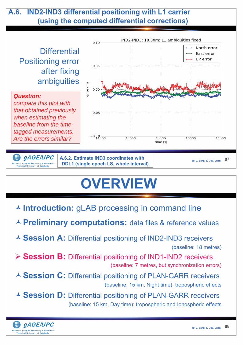
Research group of Astronomy & GeomaticsTechnical University of Catalonia
gAGE/UPC @ J. Sanz & J.M. Juan 87
Differential Positioning error
after fixing ambiguities
A.6.2. Estimate IND3 coordinates with DDL1 (single epoch LS, whole interval)
A.6. IND2-IND3 differential positioning with L1 carrier(using the computed differential corrections)
Question: compare this plot with that obtained previously when estimating the baseline from the time-tagged measurements. Are the errors similar?
Research group of Astronomy & GeomaticsTechnical University of Catalonia
gAGE/UPC @ J. Sanz & J.M. Juan
Introduction: gLAB processing in command line
Preliminary computations: data files & reference values
Session A: Differential positioning of IND2-IND3 receivers (baseline: 18 metres)
Session B: Differential positioning of IND1-IND2 receivers (baseline: 7 metres, but synchronization errors)
Session C: Differential positioning of PLAN-GARR receivers(baseline: 15 km, Night time): tropospheric effects
Session D: Differential positioning of PLAN-GARR receivers(baseline: 15 km, Day time): tropospheric and Ionospheric effects
OVERVIEW
88
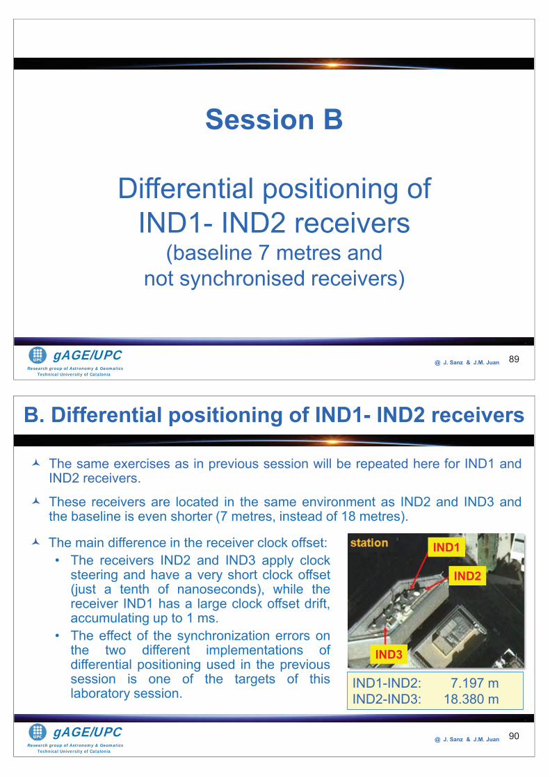
Research group of Astronomy & GeomaticsTechnical University of Catalonia
gAGE/UPC @ J. Sanz & J.M. Juan 89
Session B
Differential positioning of IND1- IND2 receivers
(baseline 7 metres andnot synchronised receivers)
Research group of Astronomy & GeomaticsTechnical University of Catalonia
gAGE/UPC @ J. Sanz & J.M. Juan 90
The same exercises as in previous session will be repeated here for IND1 andIND2 receivers.
These receivers are located in the same environment as IND2 and IND3 andthe baseline is even shorter (7 metres, instead of 18 metres).
B. Differential positioning of IND1- IND2 receivers
The main difference in the receiver clock offset:• The receivers IND2 and IND3 apply clock
steering and have a very short clock offset(just a tenth of nanoseconds), while thereceiver IND1 has a large clock offset drift,accumulating up to 1 ms.
• The effect of the synchronization errors onthe two different implementations ofdifferential positioning used in the previoussession is one of the targets of thislaboratory session.
900000000909090909999990909009090009099909090090900909099900909009090909090000999009090900900900900090090009000090900900090999009000000909000090090000090000099990009000900090009909
IND1
IND2
IND3
IND1-IND2: 7.197 mIND2-IND3: 18.380 m
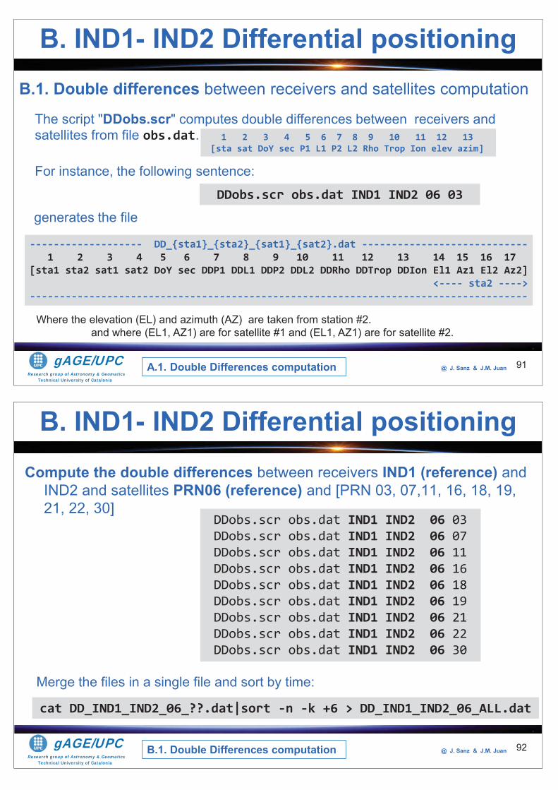
Research group of Astronomy & GeomaticsTechnical University of Catalonia
gAGE/UPC @ J. Sanz & J.M. Juan
B.1. Double differences between receivers and satellites computation
91
B. IND1- IND2 Differential positioning
1 2 3 4 5 6 7 8 9 10 11 12 13[sta sat DoY sec P1 L1 P2 L2 Rho Trop Ion elev azim]
DDobs.scr obs.dat IND1 IND2 06 03
------------------- DD_{sta1}_{sta2}_{sat1}_{sat2}.dat ----------------------------1 2 3 4 5 6 7 8 9 10 11 12 13 14 15 16 17
[sta1 sta2 sat1 sat2 DoY sec DDP1 DDL1 DDP2 DDL2 DDRho DDTrop DDIon El1 Az1 El2 Az2]<---- sta2 ---->
------------------------------------------------------------------------------------
generates the file
Where the elevation (EL) and azimuth (AZ) are taken from station #2.and where (EL1, AZ1) are for satellite #1 and (EL1, AZ1) are for satellite #2.
A.1. Double Differences computation
The script "DDobs.scr" computes double differences between receivers and satellites from file obs.dat.
For instance, the following sentence:
Research group of Astronomy & GeomaticsTechnical University of Catalonia
gAGE/UPC @ J. Sanz & J.M. Juan
Compute the double differences between receivers IND1 (reference) and IND2 and satellites PRN06 (reference) and [PRN 03, 07,11, 16, 18, 19, 21, 22, 30]
92
B. IND1- IND2 Differential positioning
DDobs.scr obs.dat IND1 IND2 06 03DDobs.scr obs.dat IND1 IND2 06 07DDobs.scr obs.dat IND1 IND2 06 11DDobs.scr obs.dat IND1 IND2 06 16DDobs.scr obs.dat IND1 IND2 06 18DDobs.scr obs.dat IND1 IND2 06 19DDobs.scr obs.dat IND1 IND2 06 21DDobs.scr obs.dat IND1 IND2 06 22DDobs.scr obs.dat IND1 IND2 06 30
Merge the files in a single file and sort by time:
cat DD_IND1_IND2_06_??.dat|sort -n -k +6 > DD_IND1_IND2_06_ALL.dat
B.1. Double Differences computation
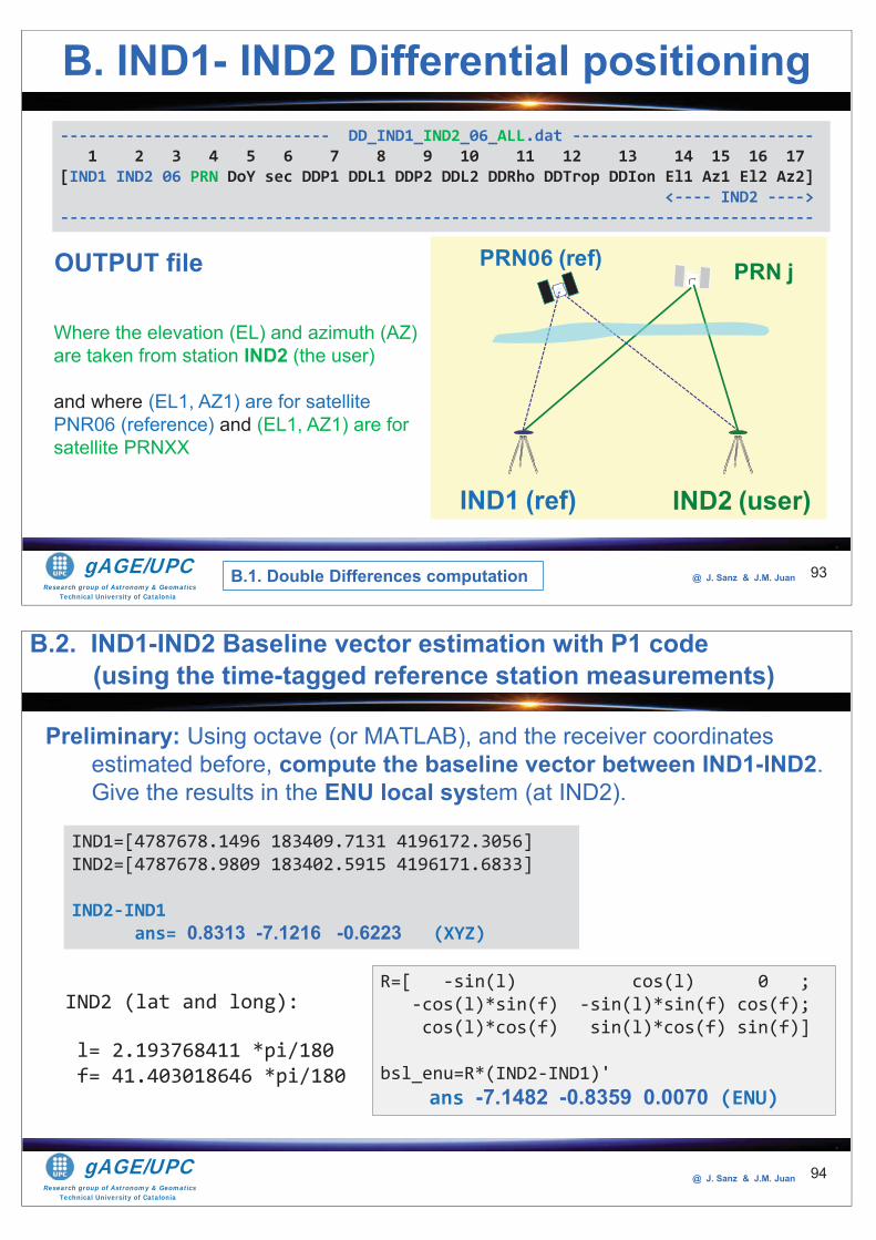
Research group of Astronomy & GeomaticsTechnical University of Catalonia
gAGE/UPC @ J. Sanz & J.M. Juan 93
----------------------------- DD_IND1_IND2_06_ALL.dat --------------------------1 2 3 4 5 6 7 8 9 10 11 12 13 14 15 16 17
[IND1 IND2 06 PRN DoY sec DDP1 DDL1 DDP2 DDL2 DDRho DDTrop DDIon El1 Az1 El2 Az2]<---- IND2 ---->
---------------------------------------------------------------------------------
OUTPUT file
Where the elevation (EL) and azimuth (AZ) are taken from station IND2 (the user)
and where (EL1, AZ1) are for satellite PNR06 (reference) and (EL1, AZ1) are for satellite PRNXX
B. IND1- IND2 Differential positioning
B.1. Double Differences computation
IND2 (user)IND1 (ref)
PRN06 (ref) PRN j
Research group of Astronomy & GeomaticsTechnical University of Catalonia
gAGE/UPC @ J. Sanz & J.M. Juan
Preliminary: Using octave (or MATLAB), and the receiver coordinates estimated before, compute the baseline vector between IND1-IND2. Give the results in the ENU local system (at IND2).
94
IND1=[4787678.1496 183409.7131 4196172.3056]IND2=[4787678.9809 183402.5915 4196171.6833]
IND2-IND1ans= 0.8313 -7.1216 -0.6223 (XYZ)
R=[ -sin(l) cos(l) 0 ; -cos(l)*sin(f) -sin(l)*sin(f) cos(f); cos(l)*cos(f) sin(l)*cos(f) sin(f)]
bsl_enu=R*(IND2-IND1)' ans -7.1482 -0.8359 0.0070 (ENU)
IND2 (lat and long):
l= 2.193768411 *pi/180f= 41.403018646 *pi/180
B.2. IND1-IND2 Baseline vector estimation with P1 code(using the time-tagged reference station measurements)
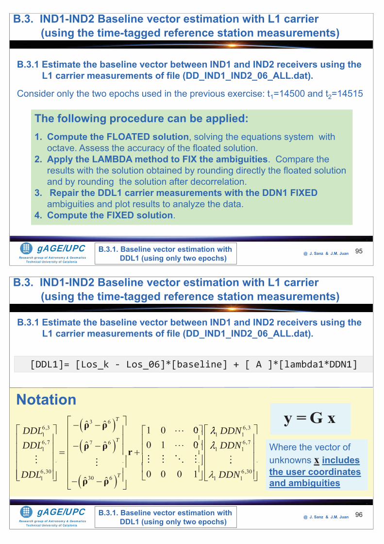
Research group of Astronomy & GeomaticsTechnical University of Catalonia
gAGE/UPC @ J. Sanz & J.M. Juan 95
B.3.1 Estimate the baseline vector between IND1 and IND2 receivers using the L1 carrier measurements of file (DD_IND1_IND2_06_ALL.dat).
Consider only the two epochs used in the previous exercise: t1=14500 and t2=14515
The following procedure can be applied:1. Compute the FLOATED solution, solving the equations system with
octave. Assess the accuracy of the floated solution.2. Apply the LAMBDA method to FIX the ambiguities. Compare the
results with the solution obtained by rounding directly the floated solution and by rounding the solution after decorrelation.
3. Repair the DDL1 carrier measurements with the DDN1 FIXED ambiguities and plot results to analyze the data.
4. Compute the FIXED solution.
B.3.1. Baseline vector estimation with DDL1 (using only two epochs)
B.3. IND1-IND2 Baseline vector estimation with L1 carrier(using the time-tagged reference station measurements)
Research group of Astronomy & GeomaticsTechnical University of Catalonia
gAGE/UPC @ J. Sanz & J.M. Juan
B.3.1 Estimate the baseline vector between IND1 and IND2 receivers using the L1 carrier measurements of file (DD_IND1_IND2_06_ALL.dat).
96
[DDL1]= [Los_k - Los_06]*[baseline] + [ A ]*[lambda1*DDN1]
3 66,3 6,31 1 16,7 6,77 61 1 1
6,30 6,3030 61 1 1
ˆ ˆ 1 0 00 1 0ˆ ˆ
0 0 0 1ˆ ˆ
00
T
T
T
DDL DDNDDL DDN
DDL DDN
ρ ρ
ρ ρ r
ρ ρ
Notation
Where the vector of unknowns x includes the user coordinates and ambiguities
y =G x
B.3. IND1-IND2 Baseline vector estimation with L1 carrier(using the time-tagged reference station measurements)
B.3.1. Baseline vector estimation with DDL1 (using only two epochs)
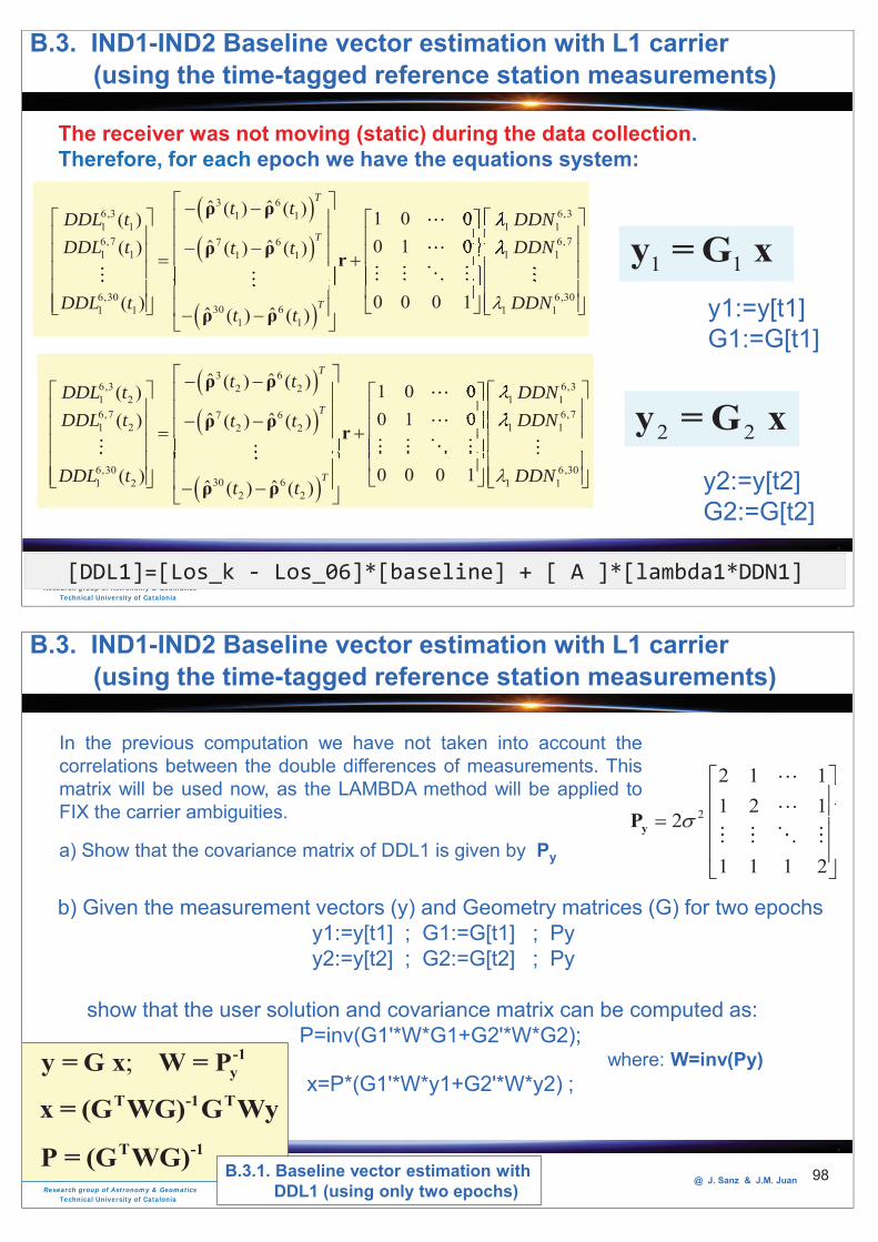
Research group of Astronomy & GeomaticsTechnical University of Catalonia
gAGE/UPC @ J. Sanz & J.M. Juan 97[DDL1]=[Los_k - Los_06]*[baseline] + [ A ]*[lambda1*DDN1]
3 66,3 6,31 11 1 1 16,7 6,77 61 1 1 11 1
6,30 6,3030 61 1 1 1
1 1
ˆ ˆ( ) ( ) 1 0 0( )0 1 0ˆ ˆ( ) ( ) ( )
0 0 0 1( ) ˆ ˆ( ) ( )
T
T
T
t tDDL t DDNDDL t DDNt t
DDL t DDNt t
ρ ρ
ρ ρ r
ρ ρ
00
3 66,3 6,32 21 2 1 16,7 6,77 61 2 1 12 2
6,30 6,3030 61 2 1 1
2 2
ˆ ˆ( ) ( ) 1 0 0( )0 1 0ˆ ˆ( ) ( ) ( )
0 0 0 1( ) ˆ ˆ( ) ( )
00
T
T
T
t tDDL t DDNDDL t DDNt t
DDL t DDNt t
ρ ρ
ρ ρ r
ρ ρ
1 1y =G xy1:=y[t1] G1:=G[t1]
2 2y = G xy2:=y[t2] G2:=G[t2]
The receiver was not moving (static) during the data collection. Therefore, for each epoch we have the equations system:
B.3. IND1-IND2 Baseline vector estimation with L1 carrier(using the time-tagged reference station measurements)
Research group of Astronomy & GeomaticsTechnical University of Catalonia
gAGE/UPC @ J. Sanz & J.M. Juan 98
In the previous computation we have not taken into account thecorrelations between the double differences of measurements. Thismatrix will be used now, as the LAMBDA method will be applied toFIX the carrier ambiguities.
a) Show that the covariance matrix of DDL1 is given by Py
2
2 1 11 2 1
2
1 1 1 2
1111
yP
b) Given the measurement vectors (y) and Geometry matrices (G) for two epochsy1:=y[t1] ; G1:=G[t1] ; Pyy2:=y[t2] ; G2:=G[t2] ; Py
show that the user solution and covariance matrix can be computed as:P=inv(G1'*W*G1+G2'*W*G2);
where: W=inv(Py)x=P*(G1'*W*y1+G2'*W*y2) ;
; -1yy = G x W = P
T -1 Tx = (G WG) G WyT -1P = (G WG)
B.3. IND1-IND2 Baseline vector estimation with L1 carrier(using the time-tagged reference station measurements)
B.3.1. Baseline vector estimation with DDL1 (using only two epochs)
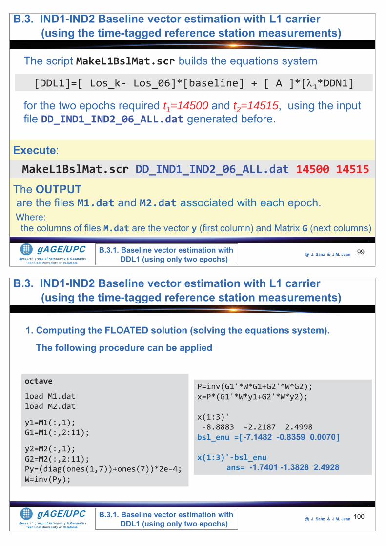
Research group of Astronomy & GeomaticsTechnical University of Catalonia
gAGE/UPC @ J. Sanz & J.M. Juan 99
The script MakeL1BslMat.scr builds the equations system
The OUTPUTare the files M1.dat and M2.dat associated with each epoch.
for the two epochs required t1=14500 and t2=14515, using the input file DD_IND1_IND2_06_ALL.dat generated before.
[DDL1]=[ Los_k- Los_06]*[baseline] + [ A ]*[ 1*DDN1]
MakeL1BslMat.scr DD_IND1_IND2_06_ALL.dat 14500 14515Execute:
Where: the columns of files M.dat are the vector y (first column) and Matrix G (next columns)
B.3. IND1-IND2 Baseline vector estimation with L1 carrier(using the time-tagged reference station measurements)
B.3.1. Baseline vector estimation with DDL1 (using only two epochs)
Research group of Astronomy & GeomaticsTechnical University of Catalonia
gAGE/UPC @ J. Sanz & J.M. Juan 100
1. Computing the FLOATED solution (solving the equations system).
The following procedure can be applied
octave
load M1.datload M2.dat
y1=M1(:,1);G1=M1(:,2:11);
y2=M2(:,1);G2=M2(:,2:11);Py=(diag(ones(1,7))+ones(7))*2e-4;W=inv(Py);
P=inv(G1'*W*G1+G2'*W*G2);x=P*(G1'*W*y1+G2'*W*y2);
x(1:3)'-8.8883 -2.2187 2.4998bsl_enu =[-7.1482 -0.8359 0.0070]
x(1:3)'-bsl_enuans= -1.7401 -1.3828 2.4928
B.3. IND1-IND2 Baseline vector estimation with L1 carrier(using the time-tagged reference station measurements)
B.3.1. Baseline vector estimation with DDL1 (using only two epochs)
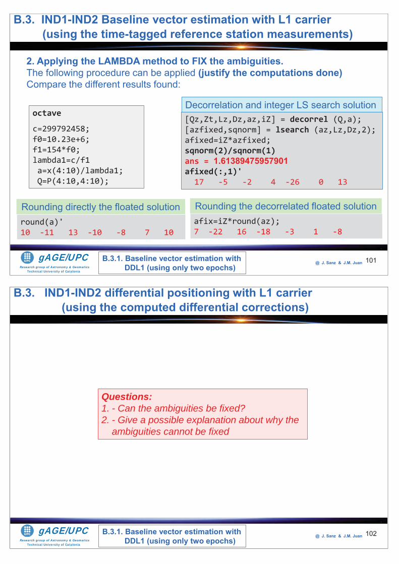
Research group of Astronomy & GeomaticsTechnical University of Catalonia
gAGE/UPC @ J. Sanz & J.M. Juan 101
octave
c=299792458;f0=10.23e+6;f1=154*f0;lambda1=c/f1a=x(4:10)/lambda1;Q=P(4:10,4:10);
afix=iZ*round(az);7 -22 16 -18 -3 1 -8
[Qz,Zt,Lz,Dz,az,iZ] = decorrel (Q,a);[azfixed,sqnorm] = lsearch (az,Lz,Dz,2);afixed=iZ*azfixed;sqnorm(2)/sqnorm(1)ans = 1.61389475957901afixed(:,1)'17 -5 -2 4 -26 0 13
Rounding the decorrelated floated solutionround(a)'10 -11 13 -10 -8 7 10
Rounding directly the floated solution
Decorrelation and integer LS search solution
B.3. IND1-IND2 Baseline vector estimation with L1 carrier(using the time-tagged reference station measurements)
B.3.1. Baseline vector estimation with DDL1 (using only two epochs)
2. Applying the LAMBDA method to FIX the ambiguities. The following procedure can be applied (justify the computations done)Compare the different results found:
Research group of Astronomy & GeomaticsTechnical University of Catalonia
gAGE/UPC @ J. Sanz & J.M. Juan 102
Questions: 1. - Can the ambiguities be fixed?2. - Give a possible explanation about why the
ambiguities cannot be fixed
B.3. IND1-IND2 differential positioning with L1 carrier(using the computed differential corrections)
B.3.1. Baseline vector estimation with DDL1 (using only two epochs)
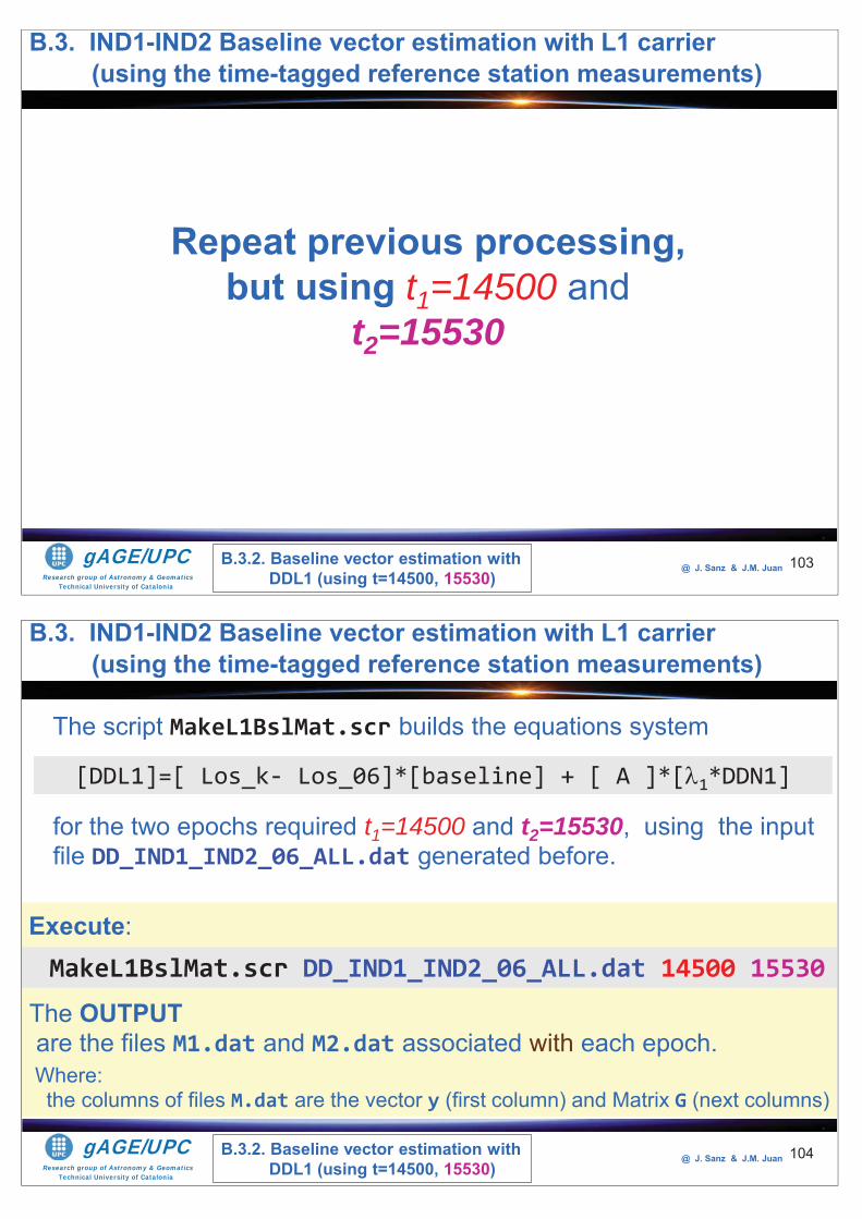
Research group of Astronomy & GeomaticsTechnical University of Catalonia
gAGE/UPC @ J. Sanz & J.M. Juan 103
B.3. IND1-IND2 Baseline vector estimation with L1 carrier(using the time-tagged reference station measurements)
B.3.2. Baseline vector estimation with DDL1 (using t=14500, 15530)
Repeat previous processing, but using t1=14500 and
t2=15530
Research group of Astronomy & GeomaticsTechnical University of Catalonia
gAGE/UPC @ J. Sanz & J.M. Juan 104
The script MakeL1BslMat.scr builds the equations system
The OUTPUTare the files M1.dat and M2.dat associated with each epoch.
for the two epochs required t1=14500 and t2=15530, using the input file DD_IND1_IND2_06_ALL.dat generated before.
[DDL1]=[ Los_k- Los_06]*[baseline] + [ A ]*[ 1*DDN1]
MakeL1BslMat.scr DD_IND1_IND2_06_ALL.dat 14500 15530Execute:
Where: the columns of files M.dat are the vector y (first column) and Matrix G (next columns)
B.3. IND1-IND2 Baseline vector estimation with L1 carrier(using the time-tagged reference station measurements)
B.3.2. Baseline vector estimation with DDL1 (using t=14500, 15530)
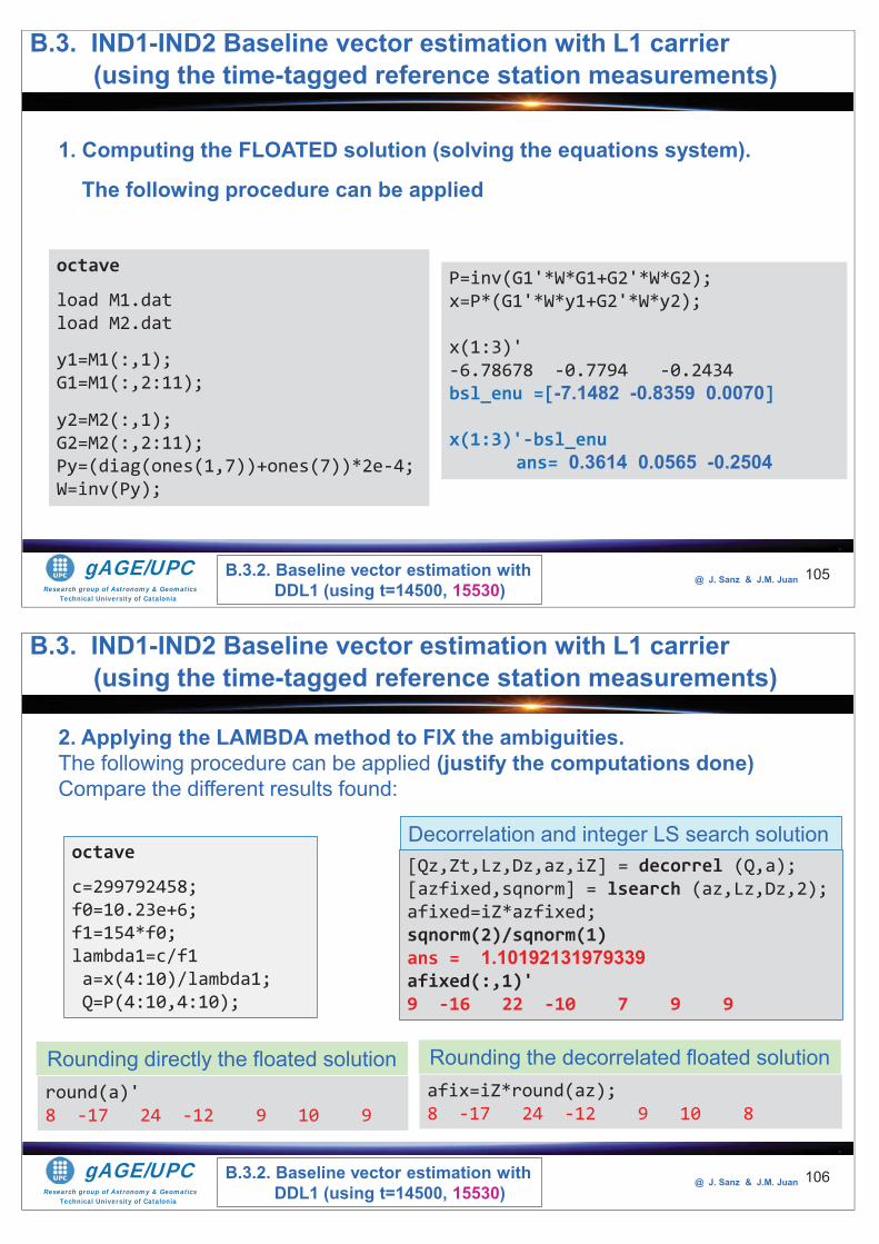
Research group of Astronomy & GeomaticsTechnical University of Catalonia
gAGE/UPC @ J. Sanz & J.M. Juan 105
1. Computing the FLOATED solution (solving the equations system).
The following procedure can be applied
octave
load M1.datload M2.dat
y1=M1(:,1);G1=M1(:,2:11);
y2=M2(:,1);G2=M2(:,2:11);Py=(diag(ones(1,7))+ones(7))*2e-4;W=inv(Py);
P=inv(G1'*W*G1+G2'*W*G2);x=P*(G1'*W*y1+G2'*W*y2);
x(1:3)'-6.78678 -0.7794 -0.2434 bsl_enu =[-7.1482 -0.8359 0.0070]
x(1:3)'-bsl_enuans= 0.3614 0.0565 -0.2504
B.3. IND1-IND2 Baseline vector estimation with L1 carrier(using the time-tagged reference station measurements)
B.3.2. Baseline vector estimation with DDL1 (using t=14500, 15530)
Research group of Astronomy & GeomaticsTechnical University of Catalonia
gAGE/UPC @ J. Sanz & J.M. Juan 106
octave
c=299792458;f0=10.23e+6;f1=154*f0;lambda1=c/f1a=x(4:10)/lambda1;Q=P(4:10,4:10);
afix=iZ*round(az);8 -17 24 -12 9 10 8
[Qz,Zt,Lz,Dz,az,iZ] = decorrel (Q,a);[azfixed,sqnorm] = lsearch (az,Lz,Dz,2);afixed=iZ*azfixed;sqnorm(2)/sqnorm(1)ans = 1.10192131979339afixed(:,1)'9 -16 22 -10 7 9 9
Rounding the decorrelated floated solutionround(a)'8 -17 24 -12 9 10 9
Rounding directly the floated solution
Decorrelation and integer LS search solution
B.3. IND1-IND2 Baseline vector estimation with L1 carrier(using the time-tagged reference station measurements)
B.3.2. Baseline vector estimation with DDL1 (using t=14500, 15530)
2. Applying the LAMBDA method to FIX the ambiguities. The following procedure can be applied (justify the computations done)Compare the different results found:
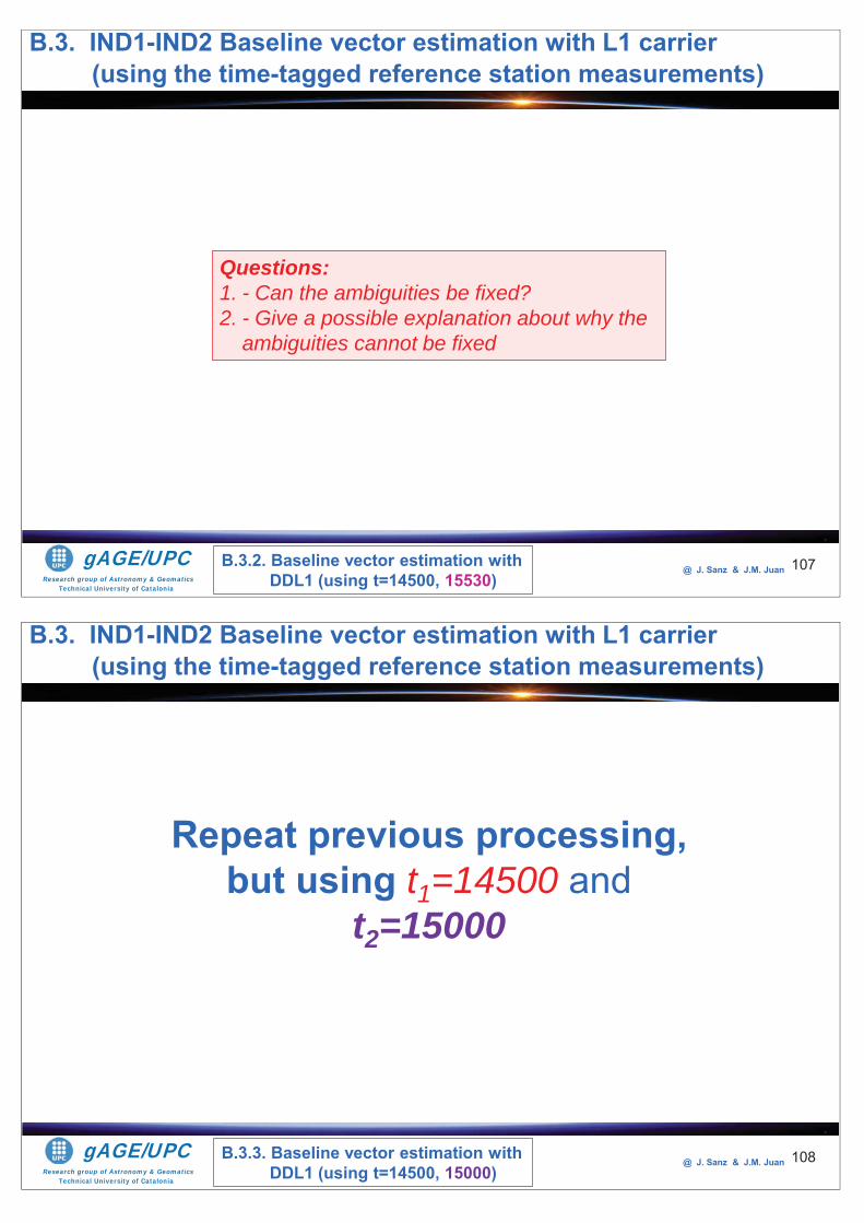
Research group of Astronomy & GeomaticsTechnical University of Catalonia
gAGE/UPC @ J. Sanz & J.M. Juan 107
Questions: 1. - Can the ambiguities be fixed? 2. - Give a possible explanation about why the
ambiguities cannot be fixed
B.3. IND1-IND2 Baseline vector estimation with L1 carrier(using the time-tagged reference station measurements)
B.3.2. Baseline vector estimation with DDL1 (using t=14500, 15530)
Research group of Astronomy & GeomaticsTechnical University of Catalonia
gAGE/UPC @ J. Sanz & J.M. Juan 108
B.3. IND1-IND2 Baseline vector estimation with L1 carrier(using the time-tagged reference station measurements)
Repeat previous processing, but using t1=14500 and
t2=15000
B.3.3. Baseline vector estimation with DDL1 (using t=14500, 15000)
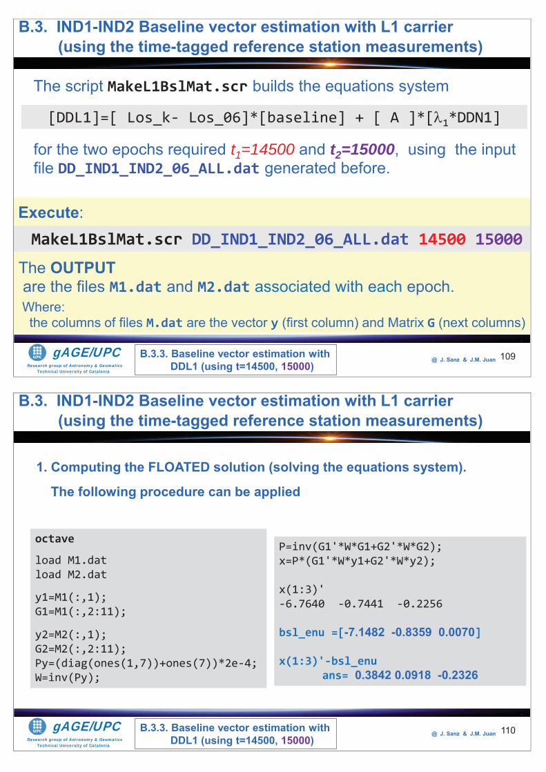
Research group of Astronomy & GeomaticsTechnical University of Catalonia
gAGE/UPC @ J. Sanz & J.M. Juan 109
The script MakeL1BslMat.scr builds the equations system
The OUTPUTare the files M1.dat and M2.dat associated with each epoch.
for the two epochs required t1=14500 and t2=15000, using the input file DD_IND1_IND2_06_ALL.dat generated before.
[DDL1]=[ Los_k- Los_06]*[baseline] + [ A ]*[ 1*DDN1]
MakeL1BslMat.scr DD_IND1_IND2_06_ALL.dat 14500 15000Execute:
Where: the columns of files M.dat are the vector y (first column) and Matrix G (next columns)
B.3. IND1-IND2 Baseline vector estimation with L1 carrier(using the time-tagged reference station measurements)
B.3.3. Baseline vector estimation with DDL1 (using t=14500, 15000)
Research group of Astronomy & GeomaticsTechnical University of Catalonia
gAGE/UPC @ J. Sanz & J.M. Juan 110
1. Computing the FLOATED solution (solving the equations system).
The following procedure can be applied
octave
load M1.datload M2.dat
y1=M1(:,1);G1=M1(:,2:11);
y2=M2(:,1);G2=M2(:,2:11);Py=(diag(ones(1,7))+ones(7))*2e-4;W=inv(Py);
P=inv(G1'*W*G1+G2'*W*G2);x=P*(G1'*W*y1+G2'*W*y2);
x(1:3)'-6.7640 -0.7441 -0.2256
bsl_enu =[-7.1482 -0.8359 0.0070]
x(1:3)'-bsl_enuans= 0.3842 0.0918 -0.2326
B.3. IND1-IND2 Baseline vector estimation with L1 carrier(using the time-tagged reference station measurements)
B.3.3. Baseline vector estimation with DDL1 (using t=14500, 15000)
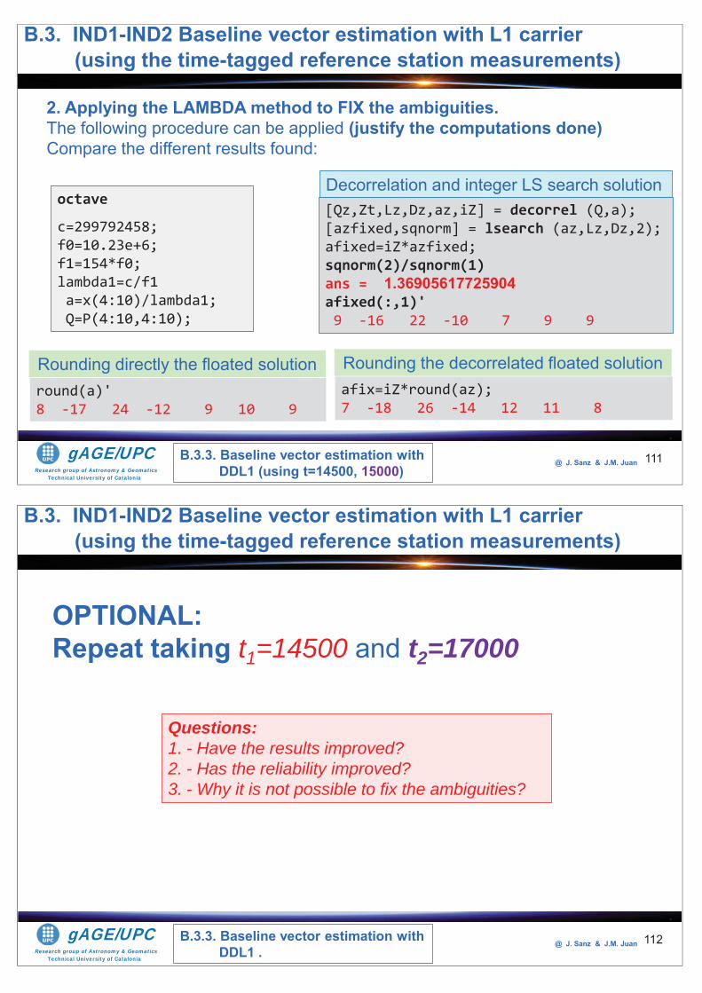
Research group of Astronomy & GeomaticsTechnical University of Catalonia
gAGE/UPC @ J. Sanz & J.M. Juan 111
octave
c=299792458;f0=10.23e+6;f1=154*f0;lambda1=c/f1a=x(4:10)/lambda1;Q=P(4:10,4:10);
afix=iZ*round(az);7 -18 26 -14 12 11 8
[Qz,Zt,Lz,Dz,az,iZ] = decorrel (Q,a);[azfixed,sqnorm] = lsearch (az,Lz,Dz,2);afixed=iZ*azfixed;sqnorm(2)/sqnorm(1)ans = 1.36905617725904afixed(:,1)'9 -16 22 -10 7 9 9
Rounding the decorrelated floated solutionround(a)'8 -17 24 -12 9 10 9
Rounding directly the floated solution
Decorrelation and integer LS search solution
B.3.3. Baseline vector estimation with DDL1 (using t=14500, 15000)
2. Applying the LAMBDA method to FIX the ambiguities. The following procedure can be applied (justify the computations done)Compare the different results found:
B.3. IND1-IND2 Baseline vector estimation with L1 carrier(using the time-tagged reference station measurements)
Research group of Astronomy & GeomaticsTechnical University of Catalonia
gAGE/UPC @ J. Sanz & J.M. Juan 112B.3.3. Baseline vector estimation with
DDL1 .
OPTIONAL:Repeat taking t1=14500 and t2=17000
Questions: 1. - Have the results improved?2. - Has the reliability improved?3. - Why it is not possible to fix the ambiguities?
B.3. IND1-IND2 Baseline vector estimation with L1 carrier(using the time-tagged reference station measurements)
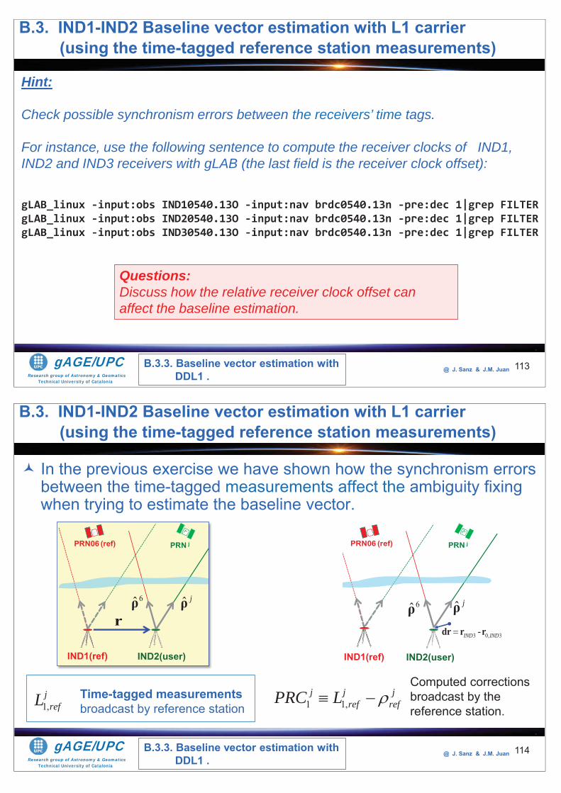
Research group of Astronomy & GeomaticsTechnical University of Catalonia
gAGE/UPC @ J. Sanz & J.M. Juan 113
Hint:
Check possible synchronism errors between the receivers’ time tags.
For instance, use the following sentence to compute the receiver clocks of IND1, IND2 and IND3 receivers with gLAB (the last field is the receiver clock offset):
gLAB_linux -input:obs IND10540.13O -input:nav brdc0540.13n -pre:dec 1|grep FILTERgLAB_linux -input:obs IND20540.13O -input:nav brdc0540.13n -pre:dec 1|grep FILTER gLAB_linux -input:obs IND30540.13O -input:nav brdc0540.13n -pre:dec 1|grep FILTER
Questions: Discuss how the relative receiver clock offset can affect the baseline estimation.
B.3.3. Baseline vector estimation with DDL1 .
B.3. IND1-IND2 Baseline vector estimation with L1 carrier(using the time-tagged reference station measurements)
Research group of Astronomy & GeomaticsTechnical University of Catalonia
gAGE/UPC @ J. Sanz & J.M. Juan 114
In the previous exercise we have shown how the synchronism errors between the time-tagged measurements affect the ambiguity fixing when trying to estimate the baseline vector.
B.3.3. Baseline vector estimation with DDL1 .
IND3 (user)IND2 (ref)
PRN06 (ref) PRN j
r
IND3 (user)IND2 (ref)
PRN06 (ref) PRN j
6ρ ˆ jρ
3 0, 3-IND INDdr r r
1 1,j j j
ref refPRC LComputed corrections broadcast by the reference station.1,
jrefL Time-tagged measurements
broadcast by reference station
6ρ ˆ jρ
B.3. IND1-IND2 Baseline vector estimation with L1 carrier(using the time-tagged reference station measurements)
IND1(ref) IND2(user) IND1(ref) IND2(user)
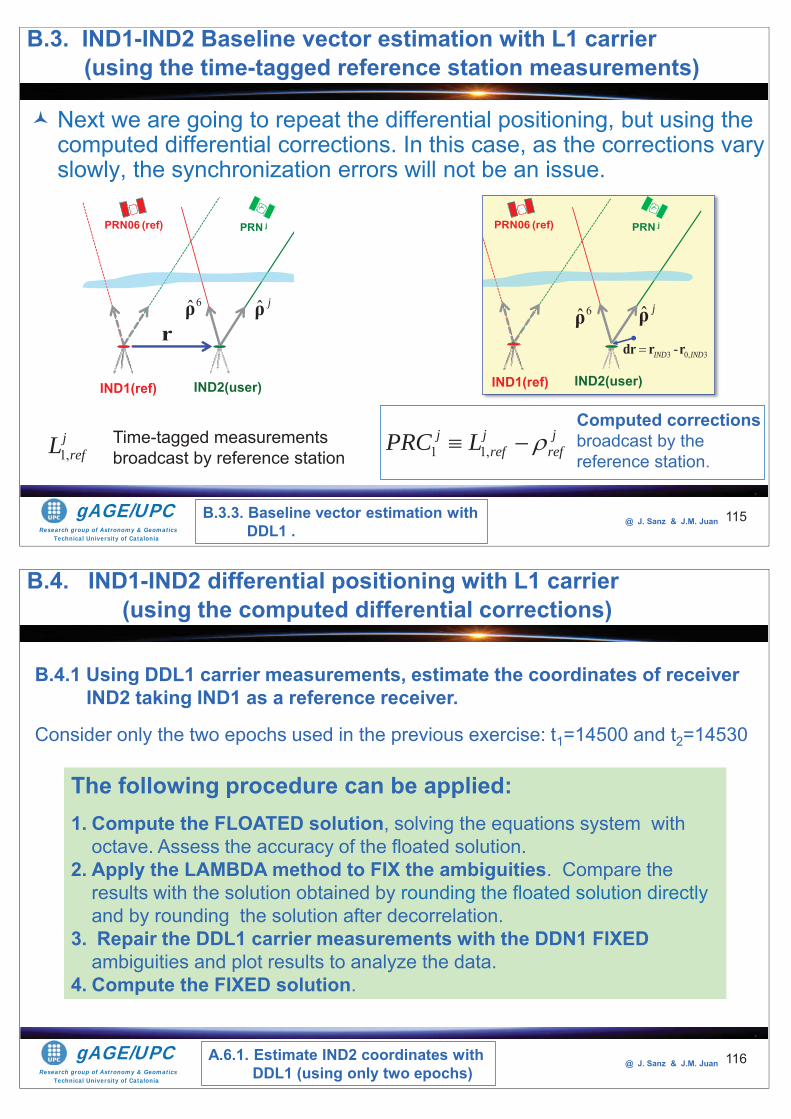
Research group of Astronomy & GeomaticsTechnical University of Catalonia
gAGE/UPC @ J. Sanz & J.M. Juan 115
Next we are going to repeat the differential positioning, but using the computed differential corrections. In this case, as the corrections vary slowly, the synchronization errors will not be an issue.
B.3.3. Baseline vector estimation with DDL1 .
IND3 (user)IND2 (ref)
PRN06 (ref) PRN j
6ρ ˆ jρr
IND3 (user)IND2 (ref)
PRN06 (ref) PRN j
6ρ3 0, 3-IND INDdr r r
1 1,j j j
ref refPRC LComputed corrections broadcast by the reference station.1,
jrefL Time-tagged measurements
broadcast by reference station
ˆ jρ
B.3. IND1-IND2 Baseline vector estimation with L1 carrier(using the time-tagged reference station measurements)
IND1(ref) IND2(user)IND1(ref) IND2(user)
Research group of Astronomy & GeomaticsTechnical University of Catalonia
gAGE/UPC @ J. Sanz & J.M. Juan 116
B.4.1 Using DDL1 carrier measurements, estimate the coordinates of receiver IND2 taking IND1 as a reference receiver.
Consider only the two epochs used in the previous exercise: t1=14500 and t2=14530
The following procedure can be applied:1. Compute the FLOATED solution, solving the equations system with
octave. Assess the accuracy of the floated solution.2. Apply the LAMBDA method to FIX the ambiguities. Compare the
results with the solution obtained by rounding the floated solution directly and by rounding the solution after decorrelation.
3. Repair the DDL1 carrier measurements with the DDN1 FIXED ambiguities and plot results to analyze the data.
4. Compute the FIXED solution.
A.6.1. Estimate IND2 coordinates with DDL1 (using only two epochs)
B.4. IND1-IND2 differential positioning with L1 carrier(using the computed differential corrections)
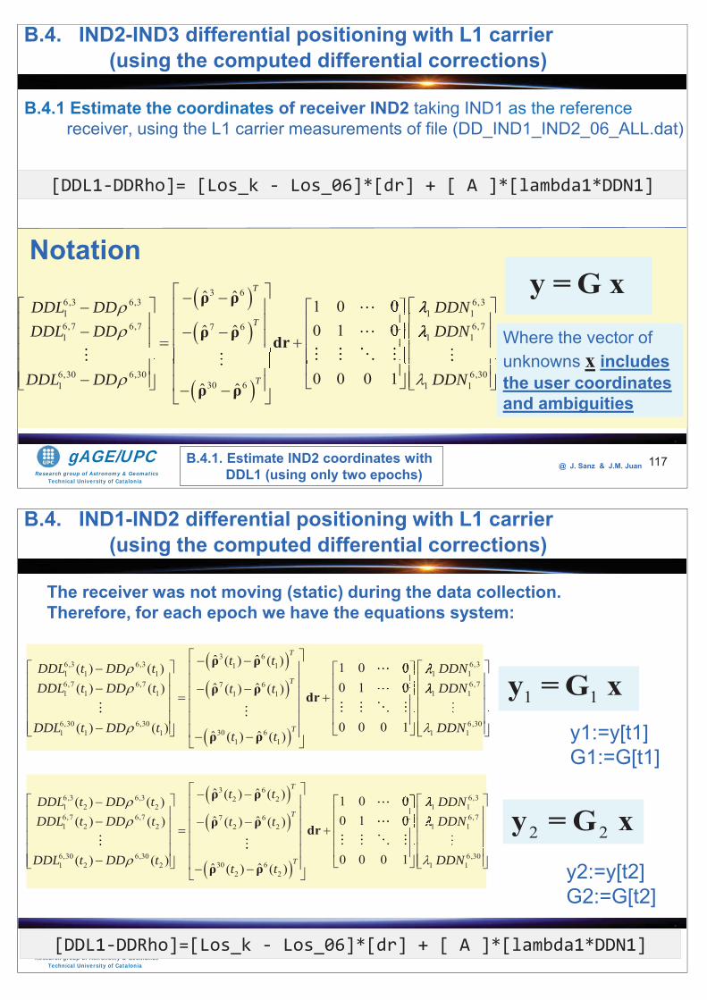
Research group of Astronomy & GeomaticsTechnical University of Catalonia
gAGE/UPC @ J. Sanz & J.M. Juan
B.4.1 Estimate the coordinates of receiver IND2 taking IND1 as the reference receiver, using the L1 carrier measurements of file (DD_IND1_IND2_06_ALL.dat)
117
[DDL1-DDRho]= [Los_k - Los_06]*[dr] + [ A ]*[lambda1*DDN1]
3 66,3 6,3 6,31 1 16,7 6,7 6,77 61 1 1
6,30 6,30 6,3030 61 1 1
ˆ ˆ 1 0 00 1 0ˆ ˆ
0 0 0 1ˆ ˆ
T
T
T
DDL DD DDNDDL DD DDN
DDL DD DDN
ρ ρ
ρ ρ dr
ρ ρ
00
Notation
Where the vector of unknowns x includes the user coordinates and ambiguities
y =G x
B.4.1. Estimate IND2 coordinates with DDL1 (using only two epochs)
B.4. IND2-IND3 differential positioning with L1 carrier(using the computed differential corrections)
Research group of Astronomy & GeomaticsTechnical University of Catalonia
gAGE/UPC @ J. Sanz & J.M. Juan 118[DDL1-DDRho]=[Los_k - Los_06]*[dr] + [ A ]*[lambda1*DDN1]
3 66,3 6,3 6,31 11 1 1 1 16,7 6,7 67 61 1 1 1 11 1
6,30 6,3030 61 1 1
1 1
ˆ ˆ( ) ( ) 1 0 0( ) ( )0 1 0ˆ ˆ( ) ( ) ( ) ( )
0 0 0 1( ) ( ) ˆ ˆ( ) ( )
T
T
T
t tDDL t DD t DDNDDL t DD t DDNt t
DDL t DD tt t
ρ ρ
ρ ρ dr
ρ ρ
00 ,7
6,301 1DDN
3 66,3 6,3 6,32 21 2 2 1 16,7 6,7 67 61 2 2 1 12 2
6,30 6,3030 61 2 2
2 2
ˆ ˆ( ) ( ) 1 0 0( ) ( )0 1 0ˆ ˆ( ) ( ) ( ) ( )
0 0 0 1( ) ( ) ˆ ˆ( ) ( )
T
T
T
t tDDL t DD t DDNDDL t DD t DDNt t
DDL t DD tt t
ρ ρ
ρ ρ dr
ρ ρ
00 ,7
6,301 1DDN
1 1y =G xy1:=y[t1] G1:=G[t1]
2 2y = G xy2:=y[t2] G2:=G[t2]
The receiver was not moving (static) during the data collection. Therefore, for each epoch we have the equations system:
B.4. IND1-IND2 differential positioning with L1 carrier(using the computed differential corrections)

Research group of Astronomy & GeomaticsTechnical University of Catalonia
gAGE/UPC @ J. Sanz & J.M. Juan 119
In the previous computation we have not taken into account thecorrelations between the double differences of measurements. Thismatrix will be used now, as the LAMBDA method will be applied toFIX the carrier ambiguities.
a) Show that the covariance matrix of DDL1 is given by Py
2
2 1 11 2 1
2
1 1 1 2
1111
yP
b) Given the measurement vectors (y) and Geometry matrices (G) for two epochsy1:=y[t1] ; G1:=G[t1] ; Pyy2:=y[t2] ; G2:=G[t2] ; Py
show that the user solution and covariance matrix can be computed as:P=inv(G1'*W*G1+G2'*W*G2);
where: W=inv(Py)x=P*(G1'*W*y1+G2'*W*y2) ;
; -1yy = G x W = P
T -1 Tx = (G WG) G WyT -1P = (G WG) B.4.1. Estimate IND2 coordinates with
DDL1 (using only two epochs)
B.4. IND1-IND2 differential positioning with L1 carrier(using the computed differential corrections)
Research group of Astronomy & GeomaticsTechnical University of Catalonia
gAGE/UPC @ J. Sanz & J.M. Juan 120
The script MakeL1DifMat.scr builds the equations system
The OUTPUTare the files M1.dat and M2.dat associated with each epoch.
for the two epochs required t1=14500 and t2=14530, using the input file DD_IND1_IND2_06_ALL.dat generated before.
[DDL1-DDRho]=[ Los_k- Los_06]*[dr] + [ A ]*[ 1*DDN1]
MakeL1DifMat.scr DD_IND1_IND2_06_ALL.dat 14500 14530Execute:
Where: the columns of files M.dat are the vector y (first column) and Matrix G (next columns)
B.41. Estimate IND2 coordinates with DDL1 (using only two epochs)
B.4. IND1-IND2 differential positioning with L1 carrier(using the computed differential corrections)
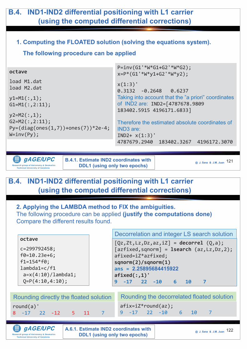
Research group of Astronomy & GeomaticsTechnical University of Catalonia
gAGE/UPC @ J. Sanz & J.M. Juan 121
1. Computing the FLOATED solution (solving the equations system).
The following procedure can be applied
octave
load M1.datload M2.dat
y1=M1(:,1);G1=M1(:,2:11);
y2=M2(:,1);G2=M2(:,2:11);Py=(diag(ones(1,7))+ones(7))*2e-4;W=inv(Py);
P=inv(G1'*W*G1+G2'*W*G2);x=P*(G1'*W*y1+G2'*W*y2);
x(1:3)'0.3132 -0.2648 0.6237Taking into account that the ”a priori” coordinates of IND2 are: IND2=[4787678.9809 183402.5915 4196171.6833]
Therefore the estimated absolute coordinates of IND3 are:IND2+ x(1:3)'4787679.2940 183402.3267 4196172.3070
B.4.1. Estimate IND2 coordinates with DDL1 (using only two epochs)
B.4. IND1-IND2 differential positioning with L1 carrier(using the computed differential corrections)
Research group of Astronomy & GeomaticsTechnical University of Catalonia
gAGE/UPC @ J. Sanz & J.M. Juan 122
octave
c=299792458;f0=10.23e+6;f1=154*f0;lambda1=c/f1a=x(4:10)/lambda1;Q=P(4:10,4:10);
afix=iZ*round(az);9 -17 22 -10 6 10 7
[Qz,Zt,Lz,Dz,az,iZ] = decorrel (Q,a);[azfixed,sqnorm] = lsearch (az,Lz,Dz,2);afixed=iZ*azfixed;sqnorm(2)/sqnorm(1)ans = 2.25895684415922afixed(:,1)'9 -17 22 -10 6 10 7
Rounding the decorrelated floated solutionround(a)'8 -17 22 -12 5 11 7
Rounding directly the floated solution
Decorrelation and integer LS search solution
A.6.1. Estimate IND2 coordinates with DDL1 (using only two epochs)
B.4. IND1-IND2 differential positioning with L1 carrier(using the computed differential corrections)
2. Applying the LAMBDA method to FIX the ambiguities. The following procedure can be applied (justify the computations done)Compare the different results found.
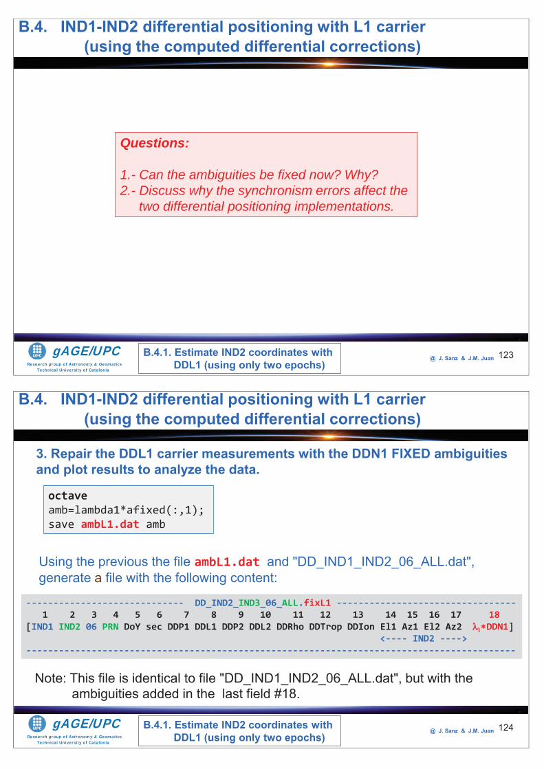
Research group of Astronomy & GeomaticsTechnical University of Catalonia
gAGE/UPC @ J. Sanz & J.M. Juan 123
Questions:
1.- Can the ambiguities be fixed now? Why?2.- Discuss why the synchronism errors affect the
two differential positioning implementations.
B.4.1. Estimate IND2 coordinates with DDL1 (using only two epochs)
B.4. IND1-IND2 differential positioning with L1 carrier(using the computed differential corrections)
Research group of Astronomy & GeomaticsTechnical University of Catalonia
gAGE/UPC @ J. Sanz & J.M. Juan 124
3. Repair the DDL1 carrier measurements with the DDN1 FIXED ambiguities and plot results to analyze the data.
octaveamb=lambda1*afixed(:,1);save ambL1.dat amb
Using the previous the file ambL1.dat and "DD_IND1_IND2_06_ALL.dat",generate a file with the following content:
----------------------------- DD_IND2_IND3_06_ALL.fixL1 ---------------------------------1 2 3 4 5 6 7 8 9 10 11 12 13 14 15 16 17 18
[IND1 IND2 06 PRN DoY sec DDP1 DDL1 DDP2 DDL2 DDRho DDTrop DDIon El1 Az1 El2 Az2 DDN1]<---- IND2 ---->
------------------------------------------------------------------------------------------
Note: This file is identical to file "DD_IND1_IND2_06_ALL.dat", but with the ambiguities added in the last field #18.
B.4.1. Estimate IND2 coordinates with DDL1 (using only two epochs)
B.4. IND1-IND2 differential positioning with L1 carrier(using the computed differential corrections)
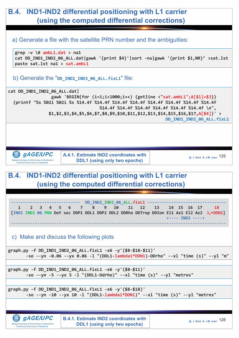
Research group of Astronomy & GeomaticsTechnical University of Catalonia
gAGE/UPC @ J. Sanz & J.M. Juan 125
grep -v \# ambL1.dat > na1cat DD_IND1_IND2_06_ALL.dat|gawk '{print $4}'|sort -nu|gawk '{print $1,NR}’ >sat.lstpaste sat.lst na1 > sat.ambL1
a) Generate a file with the satellite PRN number and the ambiguities:
cat DD_IND1_IND2_06_ALL.dat|gawk 'BEGIN{for (i=1;i<1000;i++) {getline <"sat.ambL1";A[$1]=$3}}
{printf "%s %02i %02i %s %14.4f %14.4f %14.4f %14.4f %14.4f %14.4f %14.4f %14.4f %14.4f %14.4f %14.4f %14.4f %14.4f %14.4f \n",
$1,$2,$3,$4,$5,$6,$7,$8,$9,$10,$11,$12,$13,$14,$15,$16,$17,A[$4]}' > DD_IND1_IND2_06_ALL.fixL1
b) Generate the "DD_IND2_IND3_06_ALL.fixL1" file:
A.4.1. Estimate IND2 coordinates with DDL1 (using only two epochs)
B.4. IND1-IND2 differential positioning with L1 carrier(using the computed differential corrections)
Research group of Astronomy & GeomaticsTechnical University of Catalonia
gAGE/UPC @ J. Sanz & J.M. Juan 126
graph.py -f DD_IND1_IND2_06_ALL.fixL1 -x6 -y'($8-$18-$11)' -so --yn -0.06 --yx 0.06 -l "(DDL1-lambda1*DDN1)-DDrho" --xl "time (s)" --yl "m"
c) Make and discuss the following plots
----------------------------- DD_IND2_IND3_06_ALL.fixL1 ---------------------------------1 2 3 4 5 6 7 8 9 10 11 12 13 14 15 16 17 18
[IND1 IND2 06 PRN DoY sec DDP1 DDL1 DDP2 DDL2 DDRho DDTrop DDIon El1 Az1 El2 Az2 DDN1]<---- IND2 ---->
------------------------------------------------------------------------------------------
graph.py -f DD_IND1_IND2_06_ALL.fixL1 -x6 -y'($8-$11)' -so --yn -5 --yx 5 -l "(DDL1-Ddrho)" --xl "time (s)" --yl "metres"
graph.py -f DD_IND1_IND2_06_ALL.fixL1 -x6 -y'($8-$18)' -so --yn -10 --yx 10 -l "(DDL1-lambda1*DDN1)" --xl "time (s)" --yl "metres"
B.4.1. Estimate IND2 coordinates with DDL1 (using only two epochs)
B.4. IND1-IND2 differential positioning with L1 carrier(using the computed differential corrections)
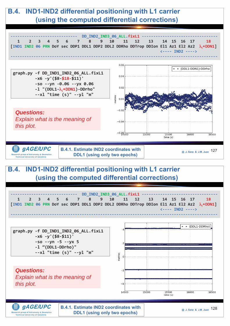
Research group of Astronomy & GeomaticsTechnical University of Catalonia
gAGE/UPC @ J. Sanz & J.M. Juan 127
graph.py -f DD_IND1_IND2_06_ALL.fixL1 -x6 -y'($8-$18-$11)' -so --yn -0.06 --yx 0.06 -l "(DDL1- DDN1)-DDrho" --xl "time (s)" --yl "m"
----------------------------- DD_IND2_IND3_06_ALL.fixL1 ---------------------------------1 2 3 4 5 6 7 8 9 10 11 12 13 14 15 16 17 18
[IND1 IND2 06 PRN DoY sec DDP1 DDL1 DDP2 DDL2 DDRho DDTrop DDIon El1 Az1 El2 Az2 DDN1]<---- IND2 ---->
------------------------------------------------------------------------------------------
B.4.1. Estimate IND2 coordinates with DDL1 (using only two epochs)
B.4. IND1-IND2 differential positioning with L1 carrier(using the computed differential corrections)
Questions:Explain what is the meaning of this plot.
Research group of Astronomy & GeomaticsTechnical University of Catalonia
gAGE/UPC @ J. Sanz & J.M. Juan 128
graph.py -f DD_IND1_IND2_06_ALL.fixL1 -x6 -y'($8-$11)' -so --yn -5 --yx 5 -l ”(DDL1-DDrho)" --xl "time (s)" --yl "m"
----------------------------- DD_IND2_IND3_06_ALL.fixL1 ---------------------------------1 2 3 4 5 6 7 8 9 10 11 12 13 14 15 16 17 18
[IND1 IND2 06 PRN DoY sec DDP1 DDL1 DDP2 DDL2 DDRho DDTrop DDIon El1 Az1 El2 Az2 DDN1]<---- IND2 ---->
------------------------------------------------------------------------------------------
B.4.1. Estimate IND2 coordinates with DDL1 (using only two epochs)
B.4. IND1-IND2 differential positioning with L1 carrier(using the computed differential corrections)
Questions:Explain what is the meaning of this plot.
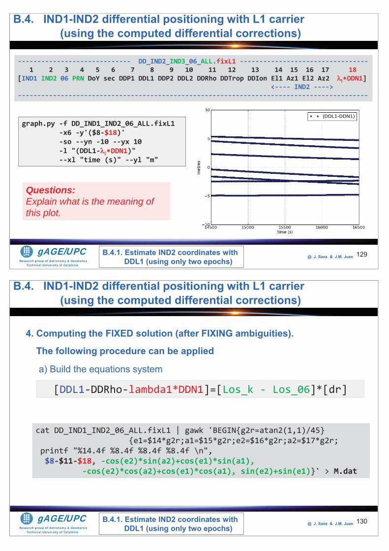
Research group of Astronomy & GeomaticsTechnical University of Catalonia
gAGE/UPC @ J. Sanz & J.M. Juan 129
graph.py -f DD_IND1_IND2_06_ALL.fixL1 -x6 -y'($8-$18)' -so --yn -10 --yx 10 -l "(DDL1- DDN1)" --xl "time (s)" --yl "m"
----------------------------- DD_IND2_IND3_06_ALL.fixL1 ---------------------------------1 2 3 4 5 6 7 8 9 10 11 12 13 14 15 16 17 18
[IND1 IND2 06 PRN DoY sec DDP1 DDL1 DDP2 DDL2 DDRho DDTrop DDIon El1 Az1 El2 Az2 DDN1]<---- IND2 ---->
------------------------------------------------------------------------------------------
B.4.1. Estimate IND2 coordinates with DDL1 (using only two epochs)
B.4. IND1-IND2 differential positioning with L1 carrier(using the computed differential corrections)
Questions:Explain what is the meaning of this plot.
Research group of Astronomy & GeomaticsTechnical University of Catalonia
gAGE/UPC @ J. Sanz & J.M. Juan 130
4. Computing the FIXED solution (after FIXING ambiguities).
The following procedure can be applied
a) Build the equations system
[DDL1-DDRho-lambda1*DDN1]=[Los_k - Los_06]*[dr]
cat DD_IND1_IND2_06_ALL.fixL1 | gawk 'BEGIN{g2r=atan2(1,1)/45} {e1=$14*g2r;a1=$15*g2r;e2=$16*g2r;a2=$17*g2r;
printf "%14.4f %8.4f %8.4f %8.4f \n",$8-$11-$18, -cos(e2)*sin(a2)+cos(e1)*sin(a1),
-cos(e2)*cos(a2)+cos(e1)*cos(a1), sin(e2)+sin(e1)}' > M.dat
B.4.1. Estimate IND2 coordinates with DDL1 (using only two epochs)
B.4. IND1-IND2 differential positioning with L1 carrier(using the computed differential corrections)
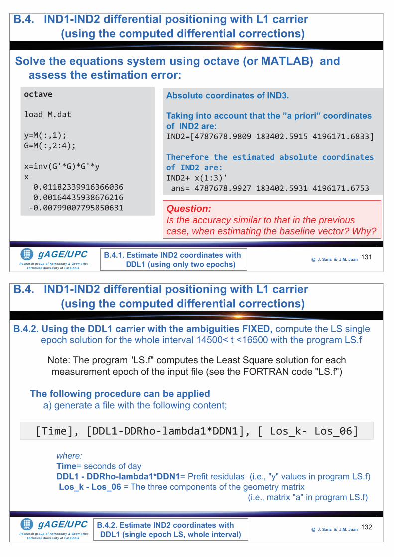
Research group of Astronomy & GeomaticsTechnical University of Catalonia
gAGE/UPC @ J. Sanz & J.M. Juan
Solve the equations system using octave (or MATLAB) and assess the estimation error:
131
octave
load M.dat
y=M(:,1);G=M(:,2:4);
x=inv(G'*G)*G'*yx0.01182339916366036 0.00164435938676216 -0.00799007795850631
Absolute coordinates of IND3.
Taking into account that the ”a priori” coordinates of IND2 are: IND2=[4787678.9809 183402.5915 4196171.6833]
Therefore the estimated absolute coordinates of IND2 are:IND2+ x(1:3)'ans= 4787678.9927 183402.5931 4196171.6753
B.4.1. Estimate IND2 coordinates with DDL1 (using only two epochs)
Question: Is the accuracy similar to that in the previous case, when estimating the baseline vector? Why?
B.4. IND1-IND2 differential positioning with L1 carrier(using the computed differential corrections)
Research group of Astronomy & GeomaticsTechnical University of Catalonia
gAGE/UPC @ J. Sanz & J.M. Juan 132
B.4.2. Using the DDL1 carrier with the ambiguities FIXED, compute the LS single epoch solution for the whole interval 14500< t <16500 with the program LS.f
Note: The program "LS.f" computes the Least Square solution for eachmeasurement epoch of the input file (see the FORTRAN code "LS.f")
The following procedure can be applieda) generate a file with the following content;
[Time], [DDL1-DDRho-lambda1*DDN1], [ Los_k- Los_06]
where:Time= seconds of day DDL1 - DDRho-lambda1*DDN1= Prefit residulas (i.e., "y" values in program LS.f)Los_k - Los_06 = The three components of the geometry matrix
(i.e., matrix "a" in program LS.f)
B.4.2. Estimate IND2 coordinates with DDL1 (single epoch LS, whole interval)
B.4. IND1-IND2 differential positioning with L1 carrier(using the computed differential corrections)
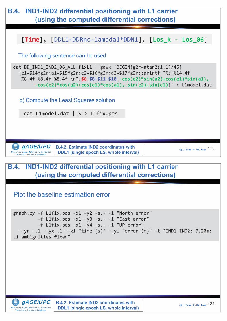
Research group of Astronomy & GeomaticsTechnical University of Catalonia
gAGE/UPC @ J. Sanz & J.M. Juan 133
The following sentence can be used
cat DD_IND1_IND2_06_ALL.fixL1 | gawk 'BEGIN{g2r=atan2(1,1)/45} {e1=$14*g2r;a1=$15*g2r;e2=$16*g2r;a2=$17*g2r;;printf "%s %14.4f%8.4f %8.4f %8.4f \n",$6,$8-$11-$18,-cos(e2)*sin(a2)+cos(e1)*sin(a1),
-cos(e2)*cos(a2)+cos(e1)*cos(a1),-sin(e2)+sin(e1)}' > L1model.dat
[Time], [DDL1-DDRho-lambda1*DDN1], [Los_k - Los_06]
b) Compute the Least Squares solution
cat L1model.dat |LS > L1fix.pos
B.4.2. Estimate IND2 coordinates with DDL1 (single epoch LS, whole interval)
B.4. IND1-IND2 differential positioning with L1 carrier(using the computed differential corrections)
Research group of Astronomy & GeomaticsTechnical University of Catalonia
gAGE/UPC @ J. Sanz & J.M. Juan 134
Plot the baseline estimation error
graph.py -f L1fix.pos -x1 –y2 -s.- -l "North error" -f L1fix.pos -x1 –y3 -s.- -l "East error" -f L1fix.pos -x1 –y4 -s.- -l "UP error"
--yn -.1 --yx .1 --xl "time (s)" --yl "error (m)" -t "IND1-IND2: 7.20m: L1 ambiguities fixed"
B.4.2. Estimate IND2 coordinates with DDL1 (single epoch LS, whole interval)
B.4. IND1-IND2 differential positioning with L1 carrier(using the computed differential corrections)
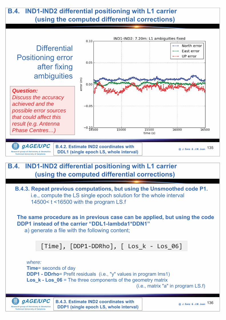
Research group of Astronomy & GeomaticsTechnical University of Catalonia
gAGE/UPC @ J. Sanz & J.M. Juan 135
Differential Positioning error
after fixing ambiguities
B.4.2. Estimate IND2 coordinates with DDL1 (single epoch LS, whole interval)
B.4. IND1-IND2 differential positioning with L1 carrier(using the computed differential corrections)
Question: Discuss the accuracy achieved and the possible error sources that could affect this result (e.g. Antenna Phase Centres…)
Research group of Astronomy & GeomaticsTechnical University of Catalonia
gAGE/UPC @ J. Sanz & J.M. Juan 136
B.4.3. Repeat previous computations, but using the Unsmoothed code P1. i.e., compute the LS single epoch solution for the whole interval 14500< t <16500 with the program LS.f
The same procedure as in previous case can be applied, but using the code DDP1 instead of the carrier “DDL1-lambda1*DDN1”
a) generate a file with the following content;
[Time], [DDP1-DDRho], [ Los_k - Los_06]
where:Time= seconds of day DDP1 - DDrho= Prefit residuals (i.e., "y" values in program lms1)Los_k - Los_06 = The three components of the geometry matrix
(i.e., matrix "a" in program LS.f)
B.4.3. Estimate IND2 coordinates with DDP1 (single epoch LS, whole interval)
B.4. IND1-IND2 differential positioning with L1 carrier(using the computed differential corrections)
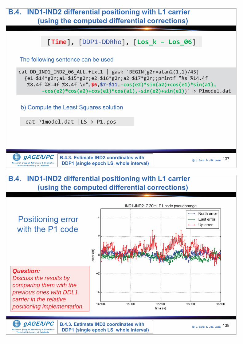
Research group of Astronomy & GeomaticsTechnical University of Catalonia
gAGE/UPC @ J. Sanz & J.M. Juan 137
The following sentence can be used
cat DD_IND1_IND2_06_ALL.fixL1 | gawk 'BEGIN{g2r=atan2(1,1)/45} {e1=$14*g2r;a1=$15*g2r;e2=$16*g2r;a2=$17*g2r;;printf "%s %14.4f%8.4f %8.4f %8.4f \n",$6,$7-$11,-cos(e2)*sin(a2)+cos(e1)*sin(a1),
-cos(e2)*cos(a2)+cos(e1)*cos(a1),-sin(e2)+sin(e1)}' > P1model.dat
[Time], [DDP1-DDRho], [Los_k – Los_06]
b) Compute the Least Squares solution
cat P1model.dat |LS > P1.pos
B.4. IND1-IND2 differential positioning with L1 carrier(using the computed differential corrections)
B.4.3. Estimate IND2 coordinates with DDP1 (single epoch LS, whole interval)
Research group of Astronomy & GeomaticsTechnical University of Catalonia
gAGE/UPC @ J. Sanz & J.M. Juan 138
Positioning error with the P1 code
B.4. IND1-IND2 differential positioning with L1 carrier(using the computed differential corrections)
B.4.3. Estimate IND2 coordinates with DDP1 (single epoch LS, whole interval)
Question: Discuss the results by comparing them with the previous ones with DDL1 carrier in the relative positioning implementation.
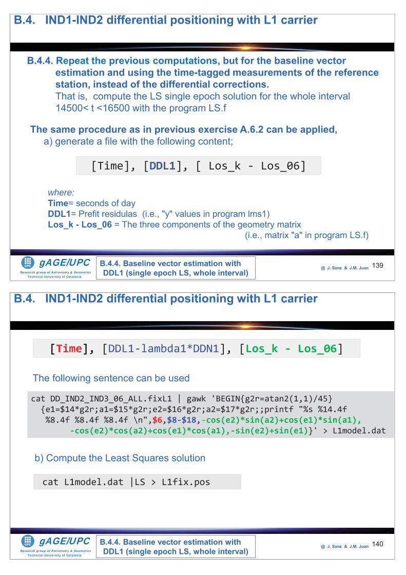
Research group of Astronomy & GeomaticsTechnical University of Catalonia
gAGE/UPC @ J. Sanz & J.M. Juan 139
B.4.4. Repeat the previous computations, but for the baseline vector estimation and using the time-tagged measurements of the reference station, instead of the differential corrections.That is, compute the LS single epoch solution for the whole interval 14500< t <16500 with the program LS.f
The same procedure as in previous exercise A.6.2 can be applied, a) generate a file with the following content;
[Time], [DDL1], [ Los_k - Los_06]
where:Time= seconds of day DDL1= Prefit residulas (i.e., "y" values in program lms1)Los_k - Los_06 = The three components of the geometry matrix
(i.e., matrix "a" in program LS.f)
B.4. IND1-IND2 differential positioning with L1 carrier
B.4.4. Baseline vector estimation with DDL1 (single epoch LS, whole interval)
Research group of Astronomy & GeomaticsTechnical University of Catalonia
gAGE/UPC @ J. Sanz & J.M. Juan 140
The following sentence can be used
cat DD_IND2_IND3_06_ALL.fixL1 | gawk 'BEGIN{g2r=atan2(1,1)/45} {e1=$14*g2r;a1=$15*g2r;e2=$16*g2r;a2=$17*g2r;;printf "%s %14.4f%8.4f %8.4f %8.4f \n",$6,$8-$18,-cos(e2)*sin(a2)+cos(e1)*sin(a1),
-cos(e2)*cos(a2)+cos(e1)*cos(a1),-sin(e2)+sin(e1)}' > L1model.dat
[Time], [DDL1-lambda1*DDN1], [Los_k - Los_06]
b) Compute the Least Squares solution
cat L1model.dat |LS > L1fix.pos
B.4.4. Baseline vector estimation with DDL1 (single epoch LS, whole interval)
B.4. IND1-IND2 differential positioning with L1 carrier
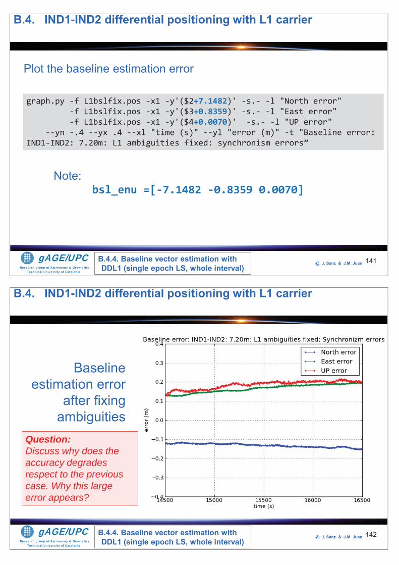
Research group of Astronomy & GeomaticsTechnical University of Catalonia
gAGE/UPC @ J. Sanz & J.M. Juan 141
Plot the baseline estimation error
graph.py -f L1bslfix.pos -x1 -y'($2+7.1482)' -s.- -l "North error" -f L1bslfix.pos -x1 -y'($3+0.8359)' -s.- -l "East error" -f L1bslfix.pos -x1 -y'($4+0.0070)' -s.- -l "UP error"
--yn -.4 --yx .4 --xl "time (s)" --yl "error (m)" -t "Baseline error: IND1-IND2: 7.20m: L1 ambiguities fixed: synchronism errors”
Note:bsl_enu =[-7.1482 -0.8359 0.0070]
B.4. IND1-IND2 differential positioning with L1 carrier
B.4.4. Baseline vector estimation with DDL1 (single epoch LS, whole interval)
Research group of Astronomy & GeomaticsTechnical University of Catalonia
gAGE/UPC @ J. Sanz & J.M. Juan 142
Baseline estimation error
after fixing ambiguities
B.4. IND1-IND2 differential positioning with L1 carrier
B.4.4. Baseline vector estimation with DDL1 (single epoch LS, whole interval)
Question: Discuss why does the accuracy degrades respect to the previous case. Why this large error appears?
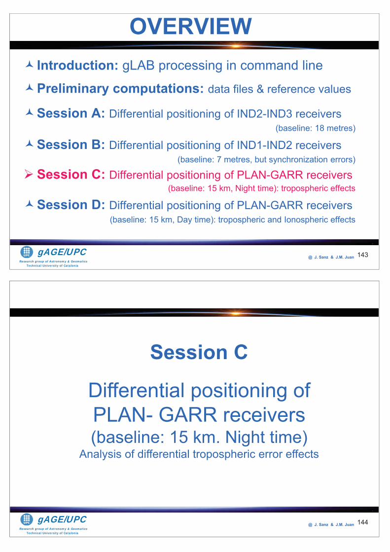
Research group of Astronomy & GeomaticsTechnical University of Catalonia
gAGE/UPC @ J. Sanz & J.M. Juan
Introduction: gLAB processing in command line
Preliminary computations: data files & reference values
Session A: Differential positioning of IND2-IND3 receivers (baseline: 18 metres)
Session B: Differential positioning of IND1-IND2 receivers (baseline: 7 metres, but synchronization errors)
Session C: Differential positioning of PLAN-GARR receivers (baseline: 15 km, Night time): tropospheric effects
Session D: Differential positioning of PLAN-GARR receivers(baseline: 15 km, Day time): tropospheric and Ionospheric effects
OVERVIEW
143
Research group of Astronomy & GeomaticsTechnical University of Catalonia
gAGE/UPC @ J. Sanz & J.M. Juan 144
Session C
Differential positioning of PLAN- GARR receivers(baseline: 15 km. Night time)
Analysis of differential tropospheric error effects
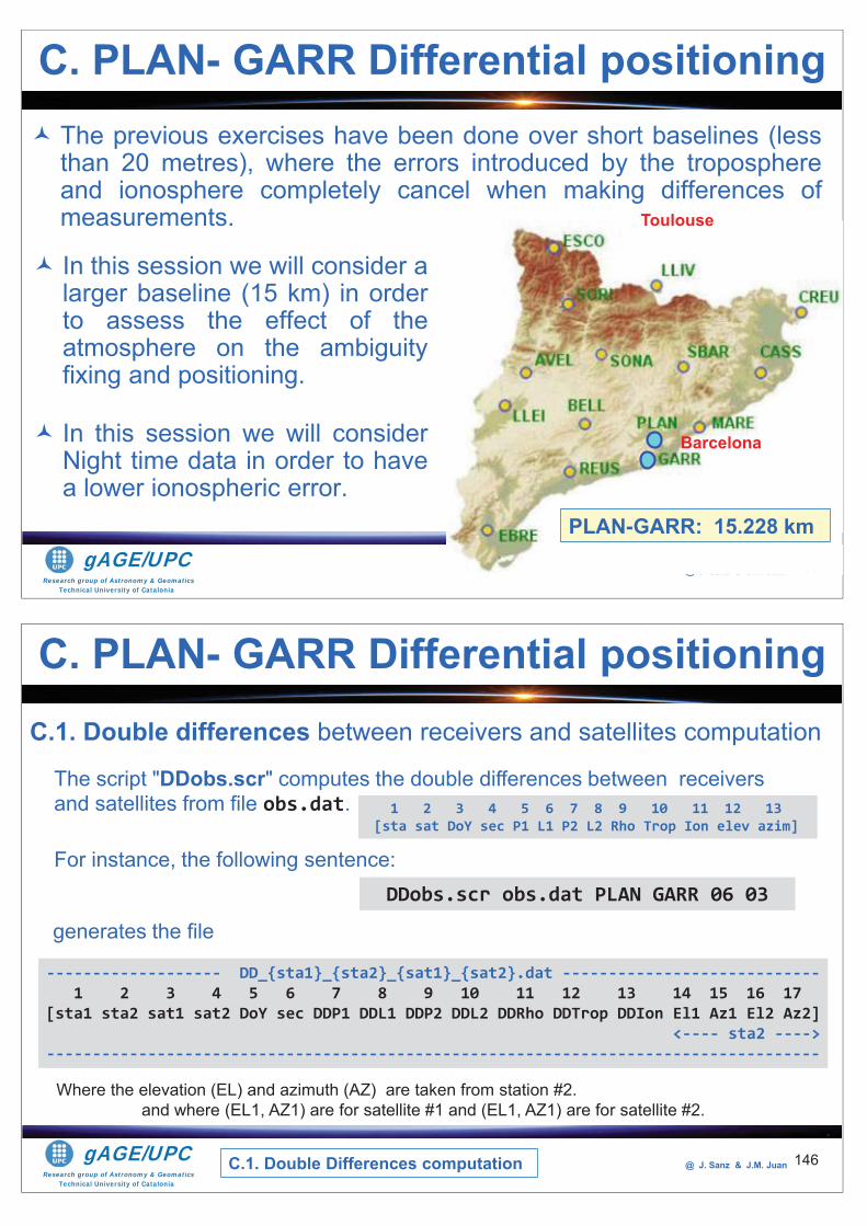
Research group of Astronomy & GeomaticsTechnical University of Catalonia
gAGE/UPC @ J. Sanz & J.M. Juan 145
The previous exercises have been done over short baselines (lessthan 20 metres), where the errors introduced by the troposphereand ionosphere completely cancel when making differences ofmeasurements.
C. PLAN- GARR Differential positioning
In this session we will consider alarger baseline (15 km) in orderto assess the effect of theatmosphere on the ambiguityfixing and positioning.
In this session we will considerNight time data in order to havea lower ionospheric error.
@ J. Sanz & J.M. Juan 145
PLAN-GARR: 15.228 km
Barcelona
Toulouse
Research group of Astronomy & GeomaticsTechnical University of Catalonia
gAGE/UPC @ J. Sanz & J.M. Juan
C.1. Double differences between receivers and satellites computation
146
C. PLAN- GARR Differential positioning
1 2 3 4 5 6 7 8 9 10 11 12 13[sta sat DoY sec P1 L1 P2 L2 Rho Trop Ion elev azim]
DDobs.scr obs.dat PLAN GARR 06 03
------------------- DD_{sta1}_{sta2}_{sat1}_{sat2}.dat ----------------------------1 2 3 4 5 6 7 8 9 10 11 12 13 14 15 16 17
[sta1 sta2 sat1 sat2 DoY sec DDP1 DDL1 DDP2 DDL2 DDRho DDTrop DDIon El1 Az1 El2 Az2]<---- sta2 ---->
------------------------------------------------------------------------------------
generates the file
Where the elevation (EL) and azimuth (AZ) are taken from station #2.and where (EL1, AZ1) are for satellite #1 and (EL1, AZ1) are for satellite #2.
C.1. Double Differences computation
The script "DDobs.scr" computes the double differences between receivers and satellites from file obs.dat.
For instance, the following sentence:
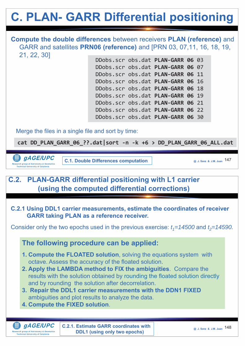
Research group of Astronomy & GeomaticsTechnical University of Catalonia
gAGE/UPC @ J. Sanz & J.M. Juan
Compute the double differences between receivers PLAN (reference) and GARR and satellites PRN06 (reference) and [PRN 03, 07,11, 16, 18, 19, 21, 22, 30]
147
C. PLAN- GARR Differential positioning
DDobs.scr obs.dat PLAN-GARR 06 03DDobs.scr obs.dat PLAN-GARR 06 07DDobs.scr obs.dat PLAN-GARR 06 11DDobs.scr obs.dat PLAN-GARR 06 16DDobs.scr obs.dat PLAN-GARR 06 18DDobs.scr obs.dat PLAN-GARR 06 19DDobs.scr obs.dat PLAN-GARR 06 21DDobs.scr obs.dat PLAN-GARR 06 22DDobs.scr obs.dat PLAN-GARR 06 30
Merge the files in a single file and sort by time:
cat DD_PLAN_GARR_06_??.dat|sort -n -k +6 > DD_PLAN_GARR_06_ALL.dat
C.1. Double Differences computation
Research group of Astronomy & GeomaticsTechnical University of Catalonia
gAGE/UPC @ J. Sanz & J.M. Juan 148
C.2.1 Using DDL1 carrier measurements, estimate the coordinates of receiver GARR taking PLAN as a reference receiver.
Consider only the two epochs used in the previous exercise: t1=14500 and t2=14590.
The following procedure can be applied:1. Compute the FLOATED solution, solving the equations system with
octave. Assess the accuracy of the floated solution.2. Apply the LAMBDA method to FIX the ambiguities. Compare the
results with the solution obtained by rounding the floated solution directly and by rounding the solution after decorrelation.
3. Repair the DDL1 carrier measurements with the DDN1 FIXED ambiguities and plot results to analyze the data.
4. Compute the FIXED solution.
C.2.1. Estimate GARR coordinates with DDL1 (using only two epochs)
C.2. PLAN-GARR differential positioning with L1 carrier(using the computed differential corrections)
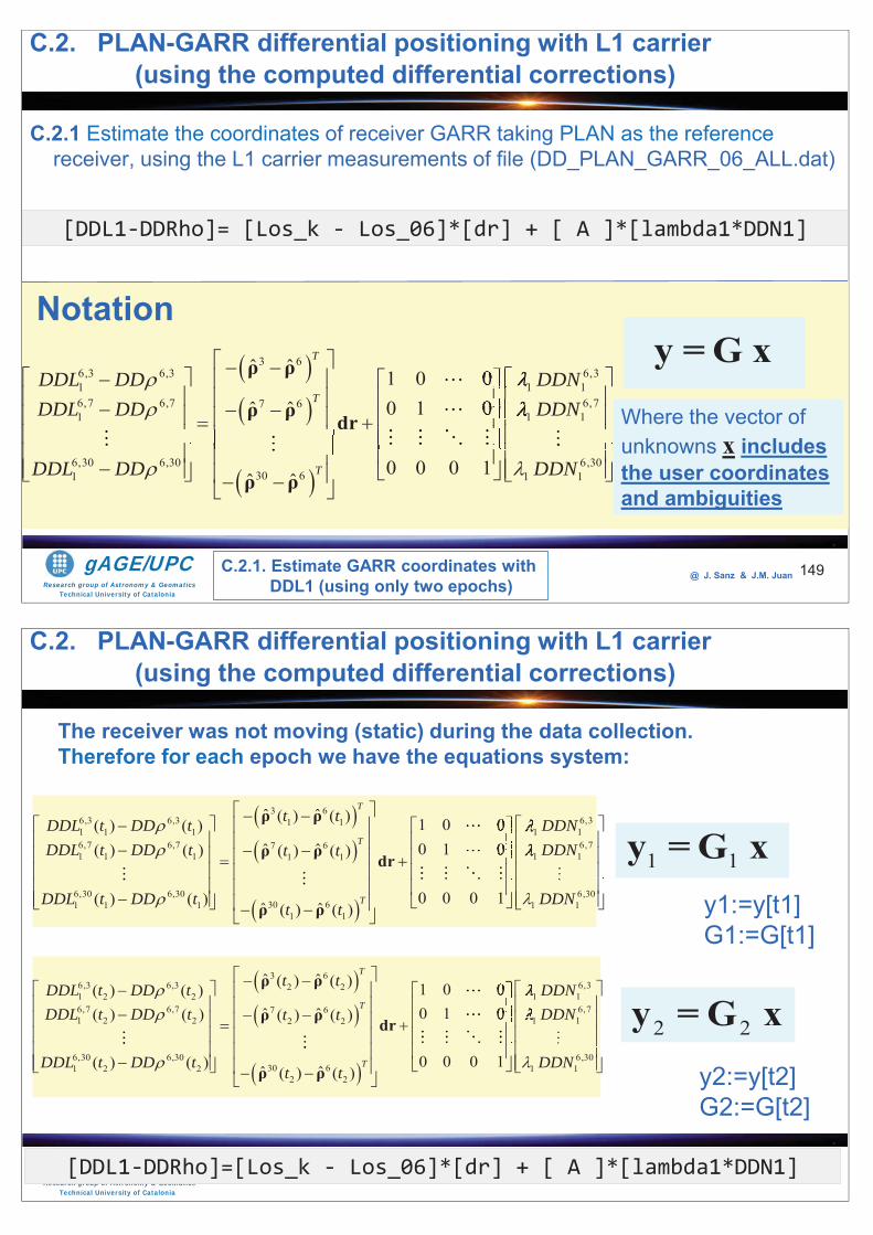
Research group of Astronomy & GeomaticsTechnical University of Catalonia
gAGE/UPC @ J. Sanz & J.M. Juan
C.2.1 Estimate the coordinates of receiver GARR taking PLAN as the reference receiver, using the L1 carrier measurements of file (DD_PLAN_GARR_06_ALL.dat)
149
[DDL1-DDRho]= [Los_k - Los_06]*[dr] + [ A ]*[lambda1*DDN1]
3 66,3 6,3 6,31 1 16,7 6,7 6,77 61 1 1
6,30 6,30 6,3030 61 1 1
ˆ ˆ 1 0 00 1 0ˆ ˆ
0 0 0 1ˆ ˆ
T
T
T
DDL DD DDNDDL DD DDN
DDL DD DDN
ρ ρ
ρ ρ dr
ρ ρ
00
Notation
Where the vector of unknowns x includes the user coordinates and ambiguities
y =G x
C.2.1. Estimate GARR coordinates with DDL1 (using only two epochs)
C.2. PLAN-GARR differential positioning with L1 carrier(using the computed differential corrections)
Research group of Astronomy & GeomaticsTechnical University of Catalonia
gAGE/UPC @ J. Sanz & J.M. Juan 150[DDL1-DDRho]=[Los_k - Los_06]*[dr] + [ A ]*[lambda1*DDN1]
3 66,3 6,3 6,31 11 1 1 1 16,7 6,7 67 61 1 1 1 11 1
6,30 6,3030 61 1 1
1 1
ˆ ˆ( ) ( ) 1 0 0( ) ( )0 1 0ˆ ˆ( ) ( ) ( ) ( )
0 0 0 1( ) ( ) ˆ ˆ( ) ( )
T
T
T
t tDDL t DD t DDNDDL t DD t DDNt t
DDL t DD tt t
ρ ρ
ρ ρ dr
ρ ρ
00 ,7
6,301 1DDN
3 66,3 6,3 6,32 21 2 2 1 16,7 6,7 67 61 2 2 1 12 2
6,30 6,3030 61 2 2
2 2
ˆ ˆ( ) ( ) 1 0 0( ) ( )0 1 0ˆ ˆ( ) ( ) ( ) ( )
0 0 0 1( ) ( ) ˆ ˆ( ) ( )
T
T
T
t tDDL t DD t DDNDDL t DD t DDNt t
DDL t DD tt t
ρ ρ
ρ ρ dr
ρ ρ
00 ,7
6,301 1DDN
1 1y =G xy1:=y[t1] G1:=G[t1]
2 2y = G xy2:=y[t2] G2:=G[t2]
The receiver was not moving (static) during the data collection. Therefore for each epoch we have the equations system:
C.2. PLAN-GARR differential positioning with L1 carrier(using the computed differential corrections)
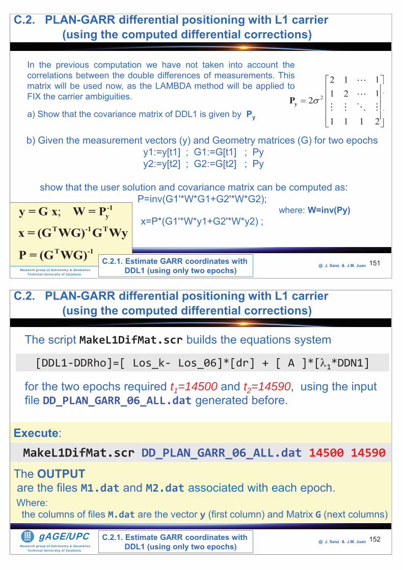
Research group of Astronomy & GeomaticsTechnical University of Catalonia
gAGE/UPC @ J. Sanz & J.M. Juan 151
In the previous computation we have not taken into account thecorrelations between the double differences of measurements. Thismatrix will be used now, as the LAMBDA method will be applied toFIX the carrier ambiguities.
a) Show that the covariance matrix of DDL1 is given by Py
2
2 1 11 2 1
2
1 1 1 2
1111
yP
b) Given the measurement vectors (y) and Geometry matrices (G) for two epochsy1:=y[t1] ; G1:=G[t1] ; Pyy2:=y[t2] ; G2:=G[t2] ; Py
show that the user solution and covariance matrix can be computed as:P=inv(G1'*W*G1+G2'*W*G2);
where: W=inv(Py)x=P*(G1'*W*y1+G2'*W*y2) ;
; -1yy = G x W = P
T -1 Tx = (G WG) G WyT -1P = (G WG) C.2.1. Estimate GARR coordinates with
DDL1 (using only two epochs)
C.2. PLAN-GARR differential positioning with L1 carrier(using the computed differential corrections)
Research group of Astronomy & GeomaticsTechnical University of Catalonia
gAGE/UPC @ J. Sanz & J.M. Juan 152
The script MakeL1DifMat.scr builds the equations system
The OUTPUTare the files M1.dat and M2.dat associated with each epoch.
for the two epochs required t1=14500 and t2=14590, using the input file DD_PLAN_GARR_06_ALL.dat generated before.
[DDL1-DDRho]=[ Los_k- Los_06]*[dr] + [ A ]*[ 1*DDN1]
MakeL1DifMat.scr DD_PLAN_GARR_06_ALL.dat 14500 14590Execute:
Where: the columns of files M.dat are the vector y (first column) and Matrix G (next columns)
C.2.1. Estimate GARR coordinates with DDL1 (using only two epochs)
C.2. PLAN-GARR differential positioning with L1 carrier(using the computed differential corrections)
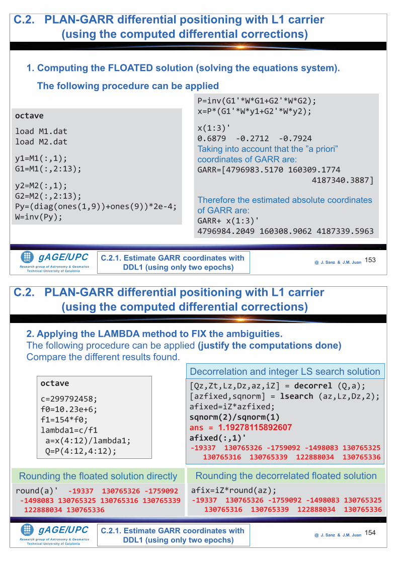
Research group of Astronomy & GeomaticsTechnical University of Catalonia
gAGE/UPC @ J. Sanz & J.M. Juan 153
1. Computing the FLOATED solution (solving the equations system).
The following procedure can be applied
octave
load M1.datload M2.dat
y1=M1(:,1);G1=M1(:,2:13);
y2=M2(:,1);G2=M2(:,2:13);Py=(diag(ones(1,9))+ones(9))*2e-4;W=inv(Py);
P=inv(G1'*W*G1+G2'*W*G2);x=P*(G1'*W*y1+G2'*W*y2);
x(1:3)'0.6879 -0.2712 -0.7924 Taking into account that the ”a priori” coordinates of GARR are: GARR=[4796983.5170 160309.1774
4187340.3887]
Therefore the estimated absolute coordinates of GARR are:GARR+ x(1:3)'4796984.2049 160308.9062 4187339.5963
C.2.1. Estimate GARR coordinates with DDL1 (using only two epochs)
C.2. PLAN-GARR differential positioning with L1 carrier(using the computed differential corrections)
Research group of Astronomy & GeomaticsTechnical University of Catalonia
gAGE/UPC @ J. Sanz & J.M. Juan 154
octave
c=299792458;f0=10.23e+6;f1=154*f0;lambda1=c/f1a=x(4:12)/lambda1;Q=P(4:12,4:12);
afix=iZ*round(az);-19337 130765326 -1759092 -1498083 130765325
130765316 130765339 122888034 130765336
[Qz,Zt,Lz,Dz,az,iZ] = decorrel (Q,a);[azfixed,sqnorm] = lsearch (az,Lz,Dz,2);afixed=iZ*azfixed;sqnorm(2)/sqnorm(1)ans = 1.19278115892607 afixed(:,1)'-19337 130765326 -1759092 -1498083 130765325
130765316 130765339 122888034 130765336
Rounding the decorrelated floated solutionround(a)' -19337 130765326 -1759092-1498083 130765325 130765316 130765339 122888034 130765336
Rounding the floated solution directly
Decorrelation and integer LS search solution
C.2.1. Estimate GARR coordinates with DDL1 (using only two epochs)
C.2. PLAN-GARR differential positioning with L1 carrier(using the computed differential corrections)
2. Applying the LAMBDA method to FIX the ambiguities. The following procedure can be applied (justify the computations done)Compare the different results found.
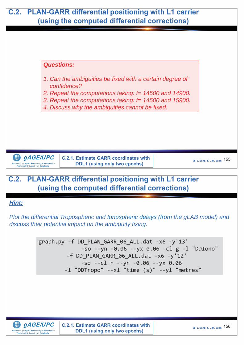
Research group of Astronomy & GeomaticsTechnical University of Catalonia
gAGE/UPC @ J. Sanz & J.M. Juan 155
Questions:
1. Can the ambiguities be fixed with a certain degree of confidence?
2. Repeat the computations taking: t= 14500 and 14900.3. Repeat the computations taking: t= 14500 and 15900.4. Discuss why the ambiguities cannot be fixed.
C.2.1. Estimate GARR coordinates with DDL1 (using only two epochs)
C.2. PLAN-GARR differential positioning with L1 carrier(using the computed differential corrections)
Research group of Astronomy & GeomaticsTechnical University of Catalonia
gAGE/UPC @ J. Sanz & J.M. Juan 156
Hint:
Plot the differential Tropospheric and Ionospheric delays (from the gLAB model) and discuss their potential impact on the ambiguity fixing.
graph.py -f DD_PLAN_GARR_06_ALL.dat -x6 -y'13' -so --yn -0.06 --yx 0.06 –cl g -l "DDIono"
-f DD_PLAN_GARR_06_ALL.dat -x6 -y'12' -so --cl r --yn -0.06 --yx 0.06
-l "DDTropo" --xl "time (s)" --yl "metres"
C.2.1. Estimate GARR coordinates with DDL1 (using only two epochs)
C.2. PLAN-GARR differential positioning with L1 carrier(using the computed differential corrections)
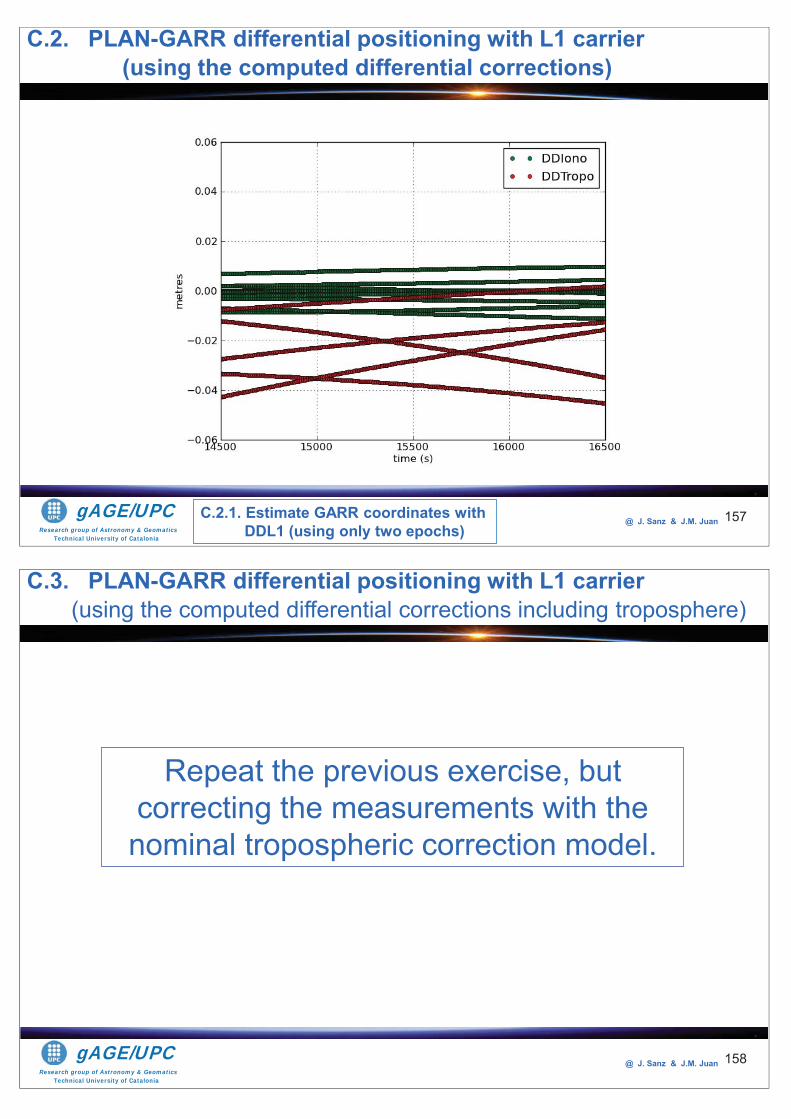
Research group of Astronomy & GeomaticsTechnical University of Catalonia
gAGE/UPC @ J. Sanz & J.M. Juan 157C.2.1. Estimate GARR coordinates with
DDL1 (using only two epochs)
C.2. PLAN-GARR differential positioning with L1 carrier(using the computed differential corrections)
Research group of Astronomy & GeomaticsTechnical University of Catalonia
gAGE/UPC @ J. Sanz & J.M. Juan 158
Repeat the previous exercise, but correcting the measurements with the nominal tropospheric correction model.
C.3. PLAN-GARR differential positioning with L1 carrier(using the computed differential corrections including troposphere)
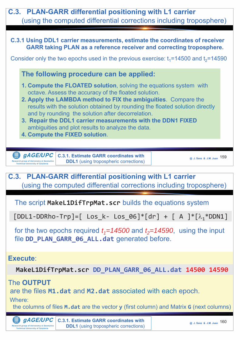
Research group of Astronomy & GeomaticsTechnical University of Catalonia
gAGE/UPC @ J. Sanz & J.M. Juan 159
C.3.1 Using DDL1 carrier measurements, estimate the coordinates of receiver GARR taking PLAN as a reference receiver and correcting troposphere.
Consider only the two epochs used in the previous exercise: t1=14500 and t2=14590
The following procedure can be applied:1. Compute the FLOATED solution, solving the equations system with
octave. Assess the accuracy of the floated solution.2. Apply the LAMBDA method to FIX the ambiguities. Compare the
results with the solution obtained by rounding the floated solution directly and by rounding the solution after decorrelation.
3. Repair the DDL1 carrier measurements with the DDN1 FIXED ambiguities and plot results to analyze the data.
4. Compute the FIXED solution.
C.3.1. Estimate GARR coordinates with DDL1 (using tropospheric corrections)
C.3. PLAN-GARR differential positioning with L1 carrier(using the computed differential corrections including troposphere)
Research group of Astronomy & GeomaticsTechnical University of Catalonia
gAGE/UPC @ J. Sanz & J.M. Juan 160
The script MakeL1DifTrpMat.scr builds the equations system
The OUTPUTare the files M1.dat and M2.dat associated with each epoch.
for the two epochs required t1=14500 and t2=14590, using the input file DD_PLAN_GARR_06_ALL.dat generated before.
[DDL1-DDRho-Trp]=[ Los_k- Los_06]*[dr] + [ A ]*[ 1*DDN1]
MakeL1DifTrpMat.scr DD_PLAN_GARR_06_ALL.dat 14500 14590
Execute:
Where: the columns of files M.dat are the vector y (first column) and Matrix G (next columns)
C.3. PLAN-GARR differential positioning with L1 carrier(using the computed differential corrections including troposphere)
C.3.1. Estimate GARR coordinates with DDL1 (using tropospheric corrections)
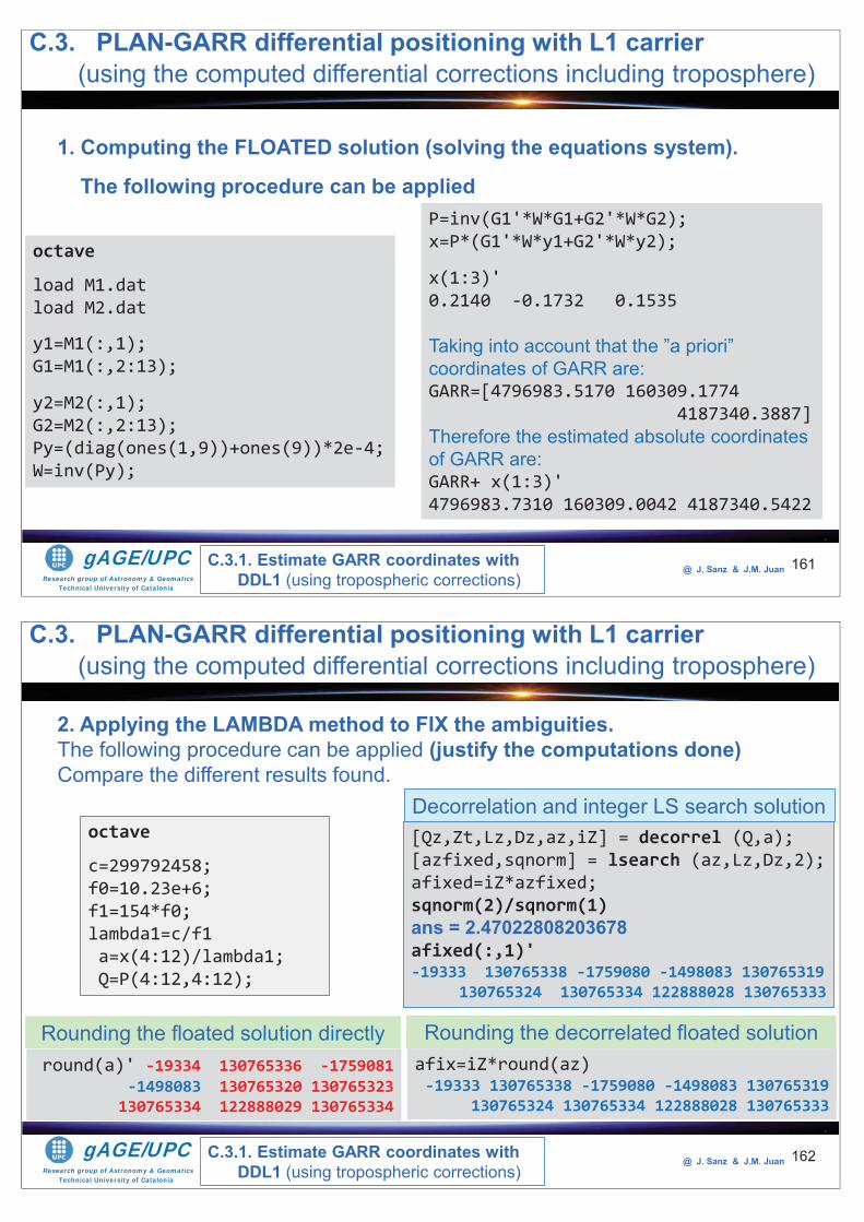
Research group of Astronomy & GeomaticsTechnical University of Catalonia
gAGE/UPC @ J. Sanz & J.M. Juan 161
1. Computing the FLOATED solution (solving the equations system).
The following procedure can be applied
octave
load M1.datload M2.dat
y1=M1(:,1);G1=M1(:,2:13);
y2=M2(:,1);G2=M2(:,2:13);Py=(diag(ones(1,9))+ones(9))*2e-4;W=inv(Py);
P=inv(G1'*W*G1+G2'*W*G2);x=P*(G1'*W*y1+G2'*W*y2);
x(1:3)'0.2140 -0.1732 0.1535
Taking into account that the ”a priori” coordinates of GARR are: GARR=[4796983.5170 160309.1774
4187340.3887]Therefore the estimated absolute coordinates of GARR are:GARR+ x(1:3)'4796983.7310 160309.0042 4187340.5422
C.3. PLAN-GARR differential positioning with L1 carrier(using the computed differential corrections including troposphere)
C.3.1. Estimate GARR coordinates with DDL1 (using tropospheric corrections)
Research group of Astronomy & GeomaticsTechnical University of Catalonia
gAGE/UPC @ J. Sanz & J.M. Juan 162
octave
c=299792458;f0=10.23e+6;f1=154*f0;lambda1=c/f1a=x(4:12)/lambda1;Q=P(4:12,4:12);
afix=iZ*round(az) -19333 130765338 -1759080 -1498083 130765319
130765324 130765334 122888028 130765333
[Qz,Zt,Lz,Dz,az,iZ] = decorrel (Q,a);[azfixed,sqnorm] = lsearch (az,Lz,Dz,2);afixed=iZ*azfixed;sqnorm(2)/sqnorm(1)ans = 2.47022808203678afixed(:,1)' -19333 130765338 -1759080 -1498083 130765319
130765324 130765334 122888028 130765333
Rounding the decorrelated floated solutionround(a)' -19334 130765336 -1759081
-1498083 130765320 130765323 130765334 122888029 130765334
Rounding the floated solution directly
Decorrelation and integer LS search solution
C.3. PLAN-GARR differential positioning with L1 carrier(using the computed differential corrections including troposphere)
C.3.1. Estimate GARR coordinates with DDL1 (using tropospheric corrections)
2. Applying the LAMBDA method to FIX the ambiguities. The following procedure can be applied (justify the computations done)Compare the different results found.
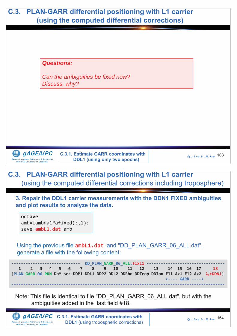
Research group of Astronomy & GeomaticsTechnical University of Catalonia
gAGE/UPC @ J. Sanz & J.M. Juan 163
Questions:
Can the ambiguities be fixed now?Discuss, why?
C.3.1. Estimate GARR coordinates with DDL1 (using only two epochs)
C.3. PLAN-GARR differential positioning with L1 carrier(using the computed differential corrections)
Research group of Astronomy & GeomaticsTechnical University of Catalonia
gAGE/UPC @ J. Sanz & J.M. Juan 164
3. Repair the DDL1 carrier measurements with the DDN1 FIXED ambiguities and plot results to analyze the data.
octaveamb=lambda1*afixed(:,1);save ambL1.dat amb
Using the previous file ambL1.dat and "DD_PLAN_GARR_06_ALL.dat",generate a file with the following content:
----------------------------- DD_PLAN_GARR_06_ALL.fixL1 ---------------------------------1 2 3 4 5 6 7 8 9 10 11 12 13 14 15 16 17 18
[PLAN GARR 06 PRN DoY sec DDP1 DDL1 DDP2 DDL2 DDRho DDTrop DDIon El1 Az1 El2 Az2 DDN1]<---- GARR ---->
------------------------------------------------------------------------------------------
Note: This file is identical to file "DD_PLAN_GARR_06_ALL.dat", but with the ambiguities added in the last field #18.
C.3. PLAN-GARR differential positioning with L1 carrier(using the computed differential corrections including troposphere)
C.3.1. Estimate GARR coordinates with DDL1 (using tropospheric corrections)
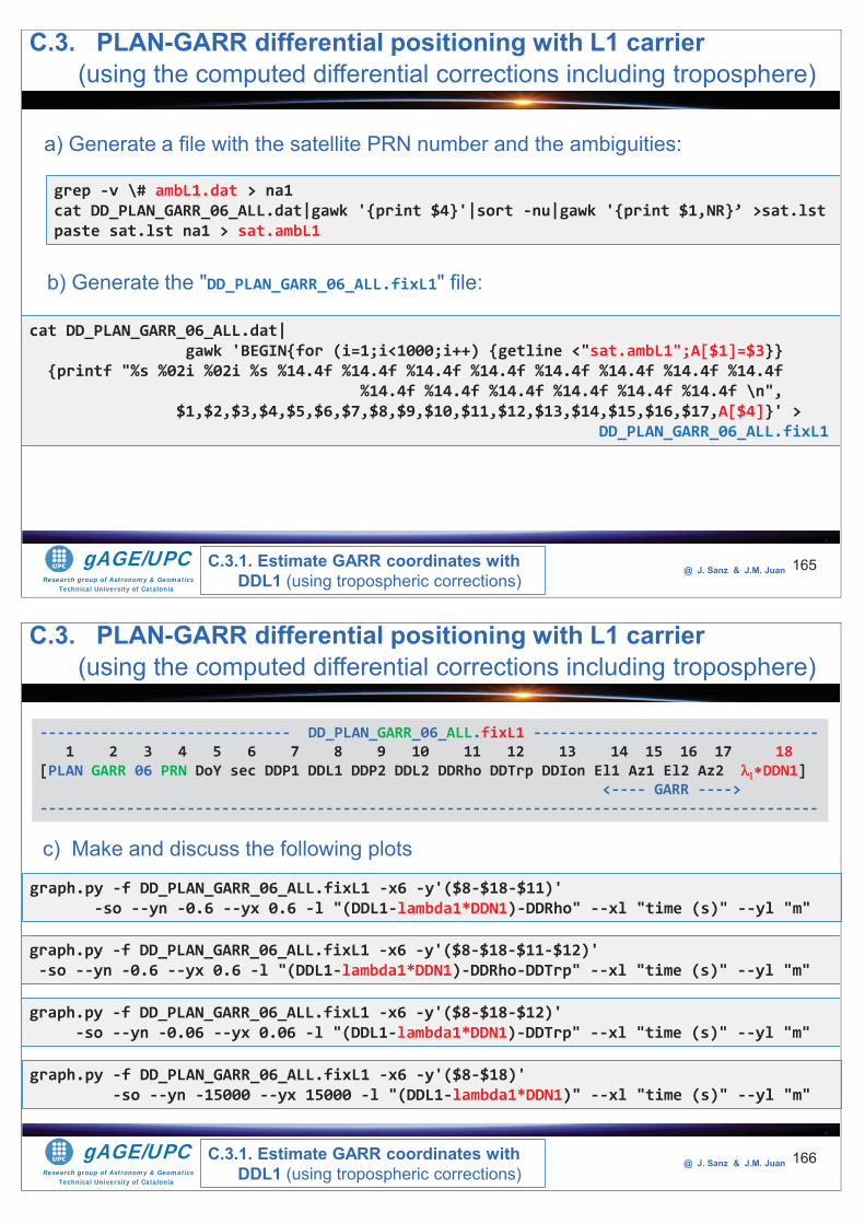
Research group of Astronomy & GeomaticsTechnical University of Catalonia
gAGE/UPC @ J. Sanz & J.M. Juan 165
grep -v \# ambL1.dat > na1cat DD_PLAN_GARR_06_ALL.dat|gawk '{print $4}'|sort -nu|gawk '{print $1,NR}’ >sat.lstpaste sat.lst na1 > sat.ambL1
a) Generate a file with the satellite PRN number and the ambiguities:
cat DD_PLAN_GARR_06_ALL.dat|gawk 'BEGIN{for (i=1;i<1000;i++) {getline <"sat.ambL1";A[$1]=$3}}
{printf "%s %02i %02i %s %14.4f %14.4f %14.4f %14.4f %14.4f %14.4f %14.4f %14.4f %14.4f %14.4f %14.4f %14.4f %14.4f %14.4f \n",
$1,$2,$3,$4,$5,$6,$7,$8,$9,$10,$11,$12,$13,$14,$15,$16,$17,A[$4]}' > DD_PLAN_GARR_06_ALL.fixL1
b) Generate the "DD_PLAN_GARR_06_ALL.fixL1" file:
C.3. PLAN-GARR differential positioning with L1 carrier(using the computed differential corrections including troposphere)
C.3.1. Estimate GARR coordinates with DDL1 (using tropospheric corrections)
Research group of Astronomy & GeomaticsTechnical University of Catalonia
gAGE/UPC @ J. Sanz & J.M. Juan 166
graph.py -f DD_PLAN_GARR_06_ALL.fixL1 -x6 -y'($8-$18-$11)' -so --yn -0.6 --yx 0.6 -l "(DDL1-lambda1*DDN1)-DDRho" --xl "time (s)" --yl "m"
c) Make and discuss the following plots
----------------------------- DD_PLAN_GARR_06_ALL.fixL1 ---------------------------------1 2 3 4 5 6 7 8 9 10 11 12 13 14 15 16 17 18
[PLAN GARR 06 PRN DoY sec DDP1 DDL1 DDP2 DDL2 DDRho DDTrp DDIon El1 Az1 El2 Az2 DDN1]<---- GARR ---->
------------------------------------------------------------------------------------------
graph.py -f DD_PLAN_GARR_06_ALL.fixL1 -x6 -y'($8-$18-$11-$12)' -so --yn -0.6 --yx 0.6 -l "(DDL1-lambda1*DDN1)-DDRho-DDTrp" --xl "time (s)" --yl "m"
C.3. PLAN-GARR differential positioning with L1 carrier(using the computed differential corrections including troposphere)
C.3.1. Estimate GARR coordinates with DDL1 (using tropospheric corrections)
graph.py -f DD_PLAN_GARR_06_ALL.fixL1 -x6 -y'($8-$18-$12)' -so --yn -0.06 --yx 0.06 -l "(DDL1-lambda1*DDN1)-DDTrp" --xl "time (s)" --yl "m"
graph.py -f DD_PLAN_GARR_06_ALL.fixL1 -x6 -y'($8-$18)' -so --yn -15000 --yx 15000 -l "(DDL1-lambda1*DDN1)" --xl "time (s)" --yl "m"
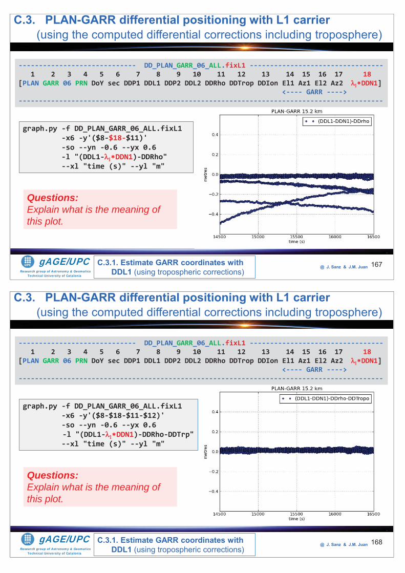
Research group of Astronomy & GeomaticsTechnical University of Catalonia
gAGE/UPC @ J. Sanz & J.M. Juan 167
graph.py -f DD_PLAN_GARR_06_ALL.fixL1 -x6 -y'($8-$18-$11)' -so --yn -0.6 --yx 0.6 -l "(DDL1- DDN1)-DDRho" --xl "time (s)" --yl "m"
C.3. PLAN-GARR differential positioning with L1 carrier(using the computed differential corrections including troposphere)
C.3.1. Estimate GARR coordinates with DDL1 (using tropospheric corrections)
----------------------------- DD_PLAN_GARR_06_ALL.fixL1 ---------------------------------1 2 3 4 5 6 7 8 9 10 11 12 13 14 15 16 17 18
[PLAN GARR 06 PRN DoY sec DDP1 DDL1 DDP2 DDL2 DDRho DDTrop DDIon El1 Az1 El2 Az2 DDN1]<---- GARR ---->
------------------------------------------------------------------------------------------
Questions:Explain what is the meaning of this plot.
Research group of Astronomy & GeomaticsTechnical University of Catalonia
gAGE/UPC @ J. Sanz & J.M. Juan 168
graph.py -f DD_PLAN_GARR_06_ALL.fixL1 -x6 -y'($8-$18-$11-$12)' -so --yn -0.6 --yx 0.6 -l "(DDL1- DDN1)-DDRho-DDTrp"--xl "time (s)" --yl "m"
C.3. PLAN-GARR differential positioning with L1 carrier(using the computed differential corrections including troposphere)
C.3.1. Estimate GARR coordinates with DDL1 (using tropospheric corrections)
----------------------------- DD_PLAN_GARR_06_ALL.fixL1 ---------------------------------1 2 3 4 5 6 7 8 9 10 11 12 13 14 15 16 17 18
[PLAN GARR 06 PRN DoY sec DDP1 DDL1 DDP2 DDL2 DDRho DDTrop DDIon El1 Az1 El2 Az2 DDN1]<---- GARR ---->
------------------------------------------------------------------------------------------
Questions:Explain what is the meaning of this plot.
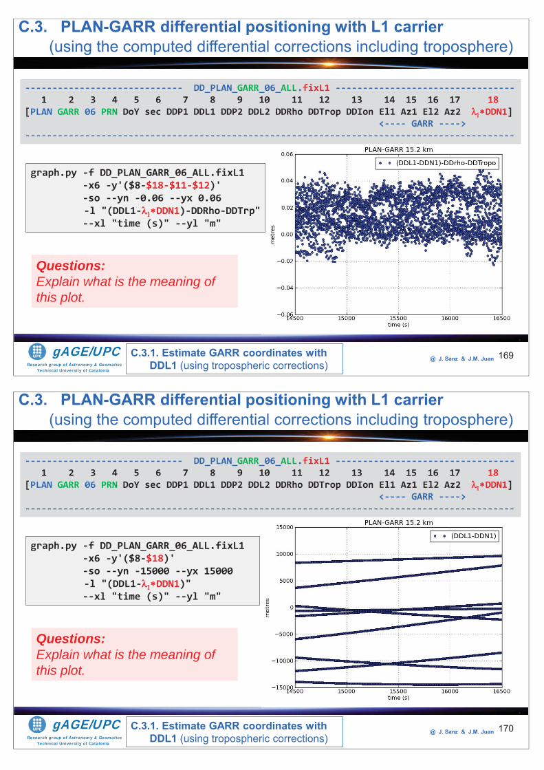
Research group of Astronomy & GeomaticsTechnical University of Catalonia
gAGE/UPC @ J. Sanz & J.M. Juan 169
graph.py -f DD_PLAN_GARR_06_ALL.fixL1 -x6 -y'($8-$18-$11-$12)' -so --yn -0.06 --yx 0.06 -l "(DDL1- DDN1)-DDRho-DDTrp"--xl "time (s)" --yl "m"
C.3. PLAN-GARR differential positioning with L1 carrier(using the computed differential corrections including troposphere)
C.3.1. Estimate GARR coordinates with DDL1 (using tropospheric corrections)
----------------------------- DD_PLAN_GARR_06_ALL.fixL1 ---------------------------------1 2 3 4 5 6 7 8 9 10 11 12 13 14 15 16 17 18
[PLAN GARR 06 PRN DoY sec DDP1 DDL1 DDP2 DDL2 DDRho DDTrop DDIon El1 Az1 El2 Az2 DDN1]<---- GARR ---->
------------------------------------------------------------------------------------------
Questions:Explain what is the meaning of this plot.
Research group of Astronomy & GeomaticsTechnical University of Catalonia
gAGE/UPC @ J. Sanz & J.M. Juan 170
graph.py -f DD_PLAN_GARR_06_ALL.fixL1 -x6 -y'($8-$18)' -so --yn -15000 --yx 15000 -l "(DDL1- DDN1)"--xl "time (s)" --yl "m"
C.3. PLAN-GARR differential positioning with L1 carrier(using the computed differential corrections including troposphere)
C.3.1. Estimate GARR coordinates with DDL1 (using tropospheric corrections)
----------------------------- DD_PLAN_GARR_06_ALL.fixL1 ---------------------------------1 2 3 4 5 6 7 8 9 10 11 12 13 14 15 16 17 18
[PLAN GARR 06 PRN DoY sec DDP1 DDL1 DDP2 DDL2 DDRho DDTrop DDIon El1 Az1 El2 Az2 DDN1]<---- GARR ---->
------------------------------------------------------------------------------------------
Questions:Explain what is the meaning of this plot.
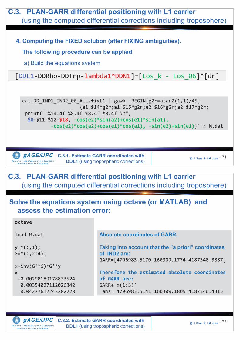
Research group of Astronomy & GeomaticsTechnical University of Catalonia
gAGE/UPC @ J. Sanz & J.M. Juan 171
4. Computing the FIXED solution (after FIXING ambiguities).
The following procedure can be applied
a) Build the equations system
[DDL1-DDRho-DDTrp-lambda1*DDN1]=[Los_k - Los_06]*[dr]
cat DD_IND1_IND2_06_ALL.fixL1 | gawk 'BEGIN{g2r=atan2(1,1)/45} {e1=$14*g2r;a1=$15*g2r;e2=$16*g2r;a2=$17*g2r;
printf "%14.4f %8.4f %8.4f %8.4f \n",$8-$11-$12-$18, -cos(e2)*sin(a2)+cos(e1)*sin(a1),
-cos(e2)*cos(a2)+cos(e1)*cos(a1), -sin(e2)+sin(e1)}' > M.dat
C.3. PLAN-GARR differential positioning with L1 carrier(using the computed differential corrections including troposphere)
C.3.1. Estimate GARR coordinates with DDL1 (using tropospheric corrections)
Research group of Astronomy & GeomaticsTechnical University of Catalonia
gAGE/UPC @ J. Sanz & J.M. Juan
Solve the equations system using octave (or MATLAB) and assess the estimation error:
172
octave
load M.dat
y=M(:,1);G=M(:,2:4);
x=inv(G'*G)*G'*yx-0.00290189178833524 0.00354027112026342 0.04277612243282228
Absolute coordinates of GARR.
Taking into account that the ”a priori” coordinates of IND2 are: GARR=[4796983.5170 160309.1774 4187340.3887]
Therefore the estimated absolute coordinates of GARR are:GARR+ x(1:3)'ans= 4796983.5141 160309.1809 4187340.4315
C.3. PLAN-GARR differential positioning with L1 carrier(using the computed differential corrections including troposphere)
C.3.2. Estimate GARR coordinates with DDL1 (using tropospheric corrections)
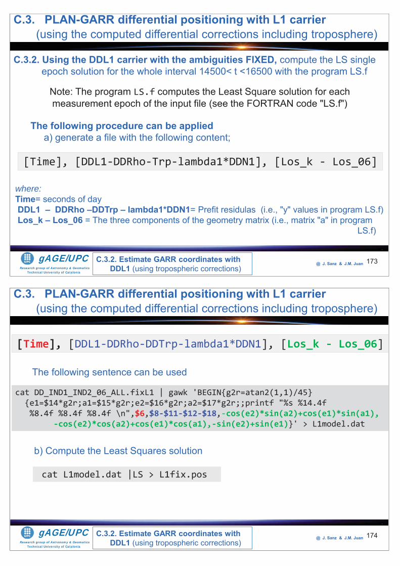
Research group of Astronomy & GeomaticsTechnical University of Catalonia
gAGE/UPC @ J. Sanz & J.M. Juan 173
C.3.2. Using the DDL1 carrier with the ambiguities FIXED, compute the LS single epoch solution for the whole interval 14500< t <16500 with the program LS.f
Note: The program LS.f computes the Least Square solution for eachmeasurement epoch of the input file (see the FORTRAN code "LS.f")
The following procedure can be applieda) generate a file with the following content;
[Time], [DDL1-DDRho-Trp-lambda1*DDN1], [Los_k - Los_06]
where:Time= seconds of day DDL1 – DDRho –DDTrp – lambda1*DDN1= Prefit residulas (i.e., "y" values in program LS.f)Los_k – Los_06 = The three components of the geometry matrix (i.e., matrix "a" in program
LS.f)
C.3. PLAN-GARR differential positioning with L1 carrier(using the computed differential corrections including troposphere)
C.3.2. Estimate GARR coordinates with DDL1 (using tropospheric corrections)
Research group of Astronomy & GeomaticsTechnical University of Catalonia
gAGE/UPC @ J. Sanz & J.M. Juan 174
The following sentence can be used
cat DD_IND1_IND2_06_ALL.fixL1 | gawk 'BEGIN{g2r=atan2(1,1)/45} {e1=$14*g2r;a1=$15*g2r;e2=$16*g2r;a2=$17*g2r;;printf "%s %14.4f%8.4f %8.4f %8.4f \n",$6,$8-$11-$12-$18,-cos(e2)*sin(a2)+cos(e1)*sin(a1),
-cos(e2)*cos(a2)+cos(e1)*cos(a1),-sin(e2)+sin(e1)}' > L1model.dat
[Time], [DDL1-DDRho-DDTrp-lambda1*DDN1], [Los_k - Los_06]
b) Compute the Least Squares solution
cat L1model.dat |LS > L1fix.pos
C.3. PLAN-GARR differential positioning with L1 carrier(using the computed differential corrections including troposphere)
C.3.2. Estimate GARR coordinates with DDL1 (using tropospheric corrections)
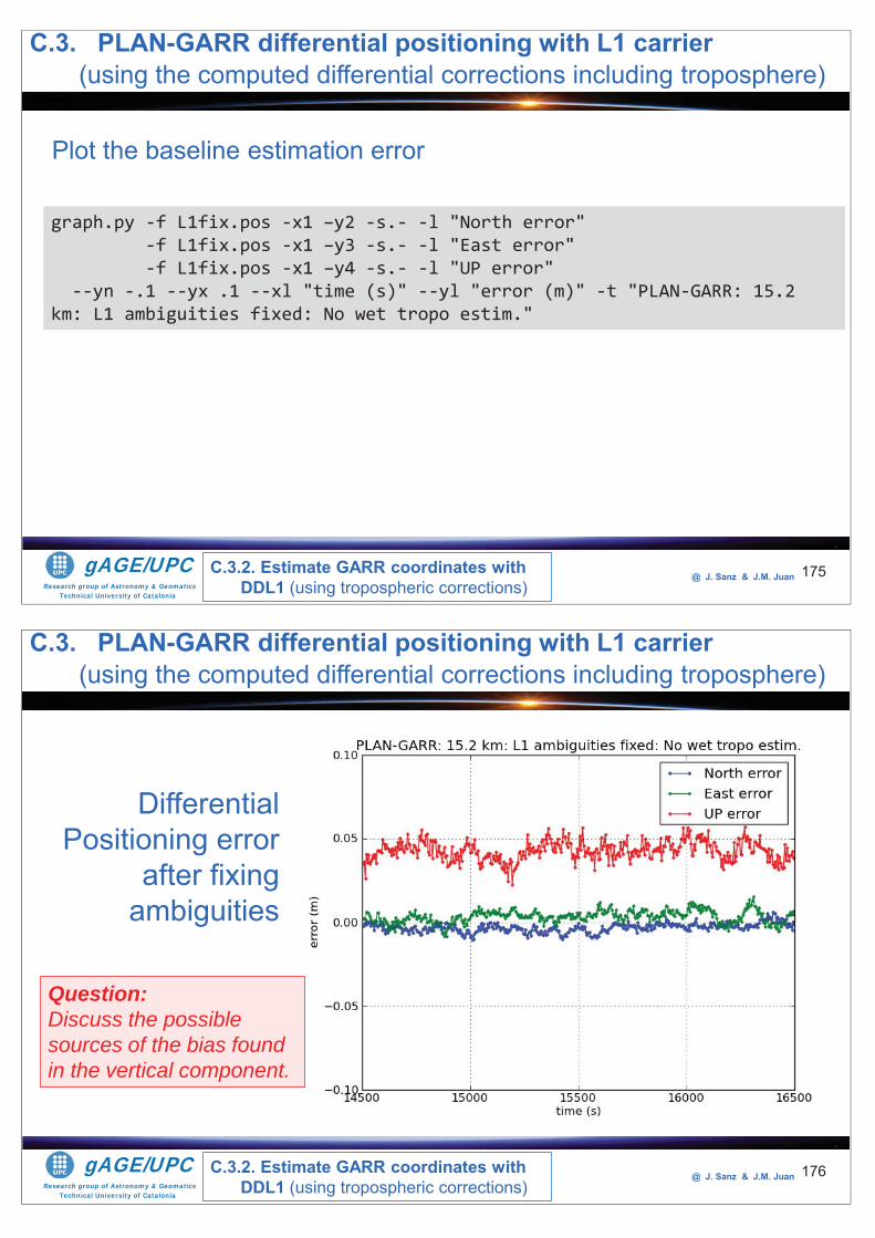
Research group of Astronomy & GeomaticsTechnical University of Catalonia
gAGE/UPC @ J. Sanz & J.M. Juan 175
Plot the baseline estimation error
graph.py -f L1fix.pos -x1 –y2 -s.- -l "North error" -f L1fix.pos -x1 –y3 -s.- -l "East error" -f L1fix.pos -x1 –y4 -s.- -l "UP error"
--yn -.1 --yx .1 --xl "time (s)" --yl "error (m)" -t "PLAN-GARR: 15.2 km: L1 ambiguities fixed: No wet tropo estim."
C.3. PLAN-GARR differential positioning with L1 carrier(using the computed differential corrections including troposphere)
C.3.2. Estimate GARR coordinates with DDL1 (using tropospheric corrections)
Research group of Astronomy & GeomaticsTechnical University of Catalonia
gAGE/UPC @ J. Sanz & J.M. Juan 176
Differential Positioning error
after fixing ambiguities
C.3. PLAN-GARR differential positioning with L1 carrier(using the computed differential corrections including troposphere)
C.3.2. Estimate GARR coordinates with DDL1 (using tropospheric corrections)
Question: Discuss the possible sources of the bias found in the vertical component.
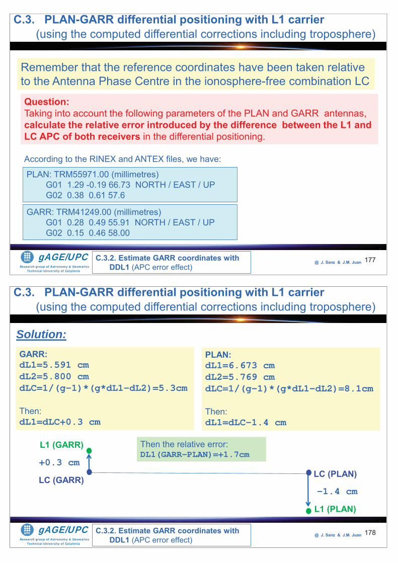
Research group of Astronomy & GeomaticsTechnical University of Catalonia
gAGE/UPC @ J. Sanz & J.M. Juan 177
C.3. PLAN-GARR differential positioning with L1 carrier(using the computed differential corrections including troposphere)
C.3.2. Estimate GARR coordinates with DDL1 (APC error effect)
Remember that the reference coordinates have been taken relative to the Antenna Phase Centre in the ionosphere-free combination LC
Question:Taking into account the following parameters of the PLAN and GARR antennas, calculate the relative error introduced by the difference between the L1 and LC APC of both receivers in the differential positioning.
According to the RINEX and ANTEX files, we have:
GARR: TRM41249.00 (millimetres)G01 0.28 0.49 55.91 NORTH / EAST / UPG02 0.15 0.46 58.00
PLAN: TRM55971.00 (millimetres)G01 1.29 -0.19 66.73 NORTH / EAST / UPG02 0.38 0.61 57.6
Research group of Astronomy & GeomaticsTechnical University of Catalonia
gAGE/UPC @ J. Sanz & J.M. Juan 178
C.3. PLAN-GARR differential positioning with L1 carrier(using the computed differential corrections including troposphere)
C.3.2. Estimate GARR coordinates with DDL1 (APC error effect)
Then the relative error:DL1(GARR-PLAN)=+1.7cm
GARR:dL1=5.591 cmdL2=5.800 cmdLC=1/(g-1)*(g*dL1-dL2)=5.3cmThen:dL1=dLC+0.3 cm
L1 (PLAN)
L1 (GARR)
LC (GARR) LC (PLAN)
PLAN:dL1=6.673 cmdL2=5.769 cmdLC=1/(g-1)*(g*dL1-dL2)=8.1cmThen:dL1=dLC-1.4 cm
+0.3 cm
-1.4 cm
Solution:
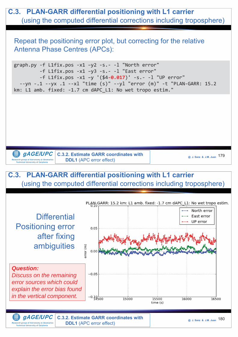
Research group of Astronomy & GeomaticsTechnical University of Catalonia
gAGE/UPC @ J. Sanz & J.M. Juan 179
Repeat the positioning error plot, but correcting for the relative Antenna Phase Centres (APCs):
graph.py -f L1fix.pos -x1 –y2 -s.- -l "North error" -f L1fix.pos -x1 –y3 -s.- -l "East error" -f L1fix.pos -x1 –y '($4-0.017)' -s.- -l "UP error"
--yn -.1 --yx .1 --xl "time (s)" --yl "error (m)" -t "PLAN-GARR: 15.2 km: L1 amb. fixed: -1.7 cm dAPC_L1: No wet tropo estim."
C.3. PLAN-GARR differential positioning with L1 carrier(using the computed differential corrections including troposphere)
C.3.2. Estimate GARR coordinates with DDL1 (APC error effect)
Research group of Astronomy & GeomaticsTechnical University of Catalonia
gAGE/UPC @ J. Sanz & J.M. Juan 180
Differential Positioning error
after fixing ambiguities
C.3. PLAN-GARR differential positioning with L1 carrier(using the computed differential corrections including troposphere)
Question: Discuss on the remaining error sources which could explain the error bias found in the vertical component.
C.3.2. Estimate GARR coordinates with DDL1 (APC error effect)
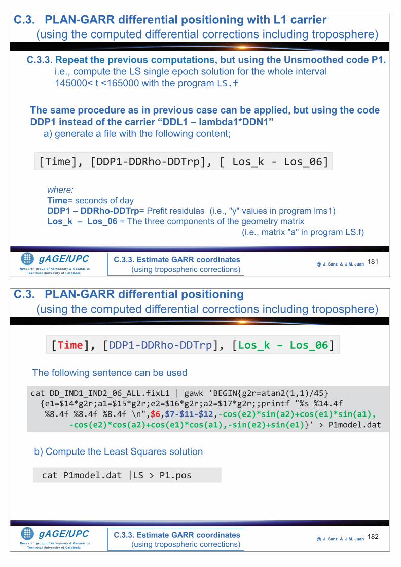
Research group of Astronomy & GeomaticsTechnical University of Catalonia
gAGE/UPC @ J. Sanz & J.M. Juan 181
C.3.3. Repeat the previous computations, but using the Unsmoothed code P1. i.e., compute the LS single epoch solution for the whole interval 145000< t <165000 with the program LS.f
The same procedure as in previous case can be applied, but using the code DDP1 instead of the carrier “DDL1 – lambda1*DDN1”
a) generate a file with the following content;
[Time], [DDP1-DDRho-DDTrp], [ Los_k - Los_06]
where:Time= seconds of day DDP1 – DDRho-DDTrp= Prefit residulas (i.e., "y" values in program lms1)Los_k – Los_06 = The three components of the geometry matrix
(i.e., matrix "a" in program LS.f)
C.3. PLAN-GARR differential positioning with L1 carrier(using the computed differential corrections including troposphere)
C.3.3. Estimate GARR coordinates (using tropospheric corrections)
Research group of Astronomy & GeomaticsTechnical University of Catalonia
gAGE/UPC @ J. Sanz & J.M. Juan 182
The following sentence can be used
cat DD_IND1_IND2_06_ALL.fixL1 | gawk 'BEGIN{g2r=atan2(1,1)/45} {e1=$14*g2r;a1=$15*g2r;e2=$16*g2r;a2=$17*g2r;;printf "%s %14.4f%8.4f %8.4f %8.4f \n",$6,$7-$11-$12,-cos(e2)*sin(a2)+cos(e1)*sin(a1),
-cos(e2)*cos(a2)+cos(e1)*cos(a1),-sin(e2)+sin(e1)}' > P1model.dat
[Time], [DDP1-DDRho-DDTrp], [Los_k – Los_06]
b) Compute the Least Squares solution
cat P1model.dat |LS > P1.pos
C.3. PLAN-GARR differential positioning (using the computed differential corrections including troposphere)
C.3.3. Estimate GARR coordinates (using tropospheric corrections)
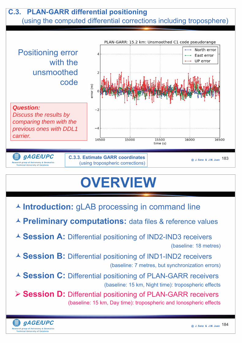
Research group of Astronomy & GeomaticsTechnical University of Catalonia
gAGE/UPC @ J. Sanz & J.M. Juan 183
Positioning error with the
unsmoothed code
Question: Discuss the results by comparing them with the previous ones with DDL1 carrier.
C.3. PLAN-GARR differential positioning (using the computed differential corrections including troposphere)
C.3.3. Estimate GARR coordinates (using tropospheric corrections)
Research group of Astronomy & GeomaticsTechnical University of Catalonia
gAGE/UPC @ J. Sanz & J.M. Juan
Introduction: gLAB processing in command line
Preliminary computations: data files & reference values
Session A: Differential positioning of IND2-IND3 receivers (baseline: 18 metres)
Session B: Differential positioning of IND1-IND2 receivers (baseline: 7 metres, but synchronization errors)
Session C: Differential positioning of PLAN-GARR receivers(baseline: 15 km, Night time): tropospheric effects
Session D: Differential positioning of PLAN-GARR receivers (baseline: 15 km, Day time): tropospheric and Ionospheric effects
OVERVIEW
184
Research group of Astronomy & GeomaticsTechnical University of Catalonia
gAGE/UPC @ J. Sanz & J.M. Juan 185
Session D
Differential positioning of PLAN- GARR receivers
(baseline: 15 km. Day time)Analysis of differential tropospheric
and Ionospheric error effects
Research group of Astronomy & GeomaticsTechnical University of Catalonia
gAGE/UPC @ J. Sanz & J.M. Juan 186
The previous session has been carried out using measurements collected during the night time, when the effect of the ionosphere is lower.The effect of the ionosphere over a baseline of 15km (and in solar maximum conditions) will be assessed in this session using day-time measurements.The exercise will end with the computation of the unambiguous DDSTEC from dual-frequency carrier measurements (after fixing the ambiguities in both carriers).The solutions computed using the DDL1 carrier (with the ambiguity fixed) corrected by the unambiguous DDSTEC and corrected by the nominal Klobuchar model will be compared.Finally, the solution using the unambiguous DDLC carrier (iono-free combination) will be also computed to compare results.
D. Differential positioning of PLAN-GARR receivers
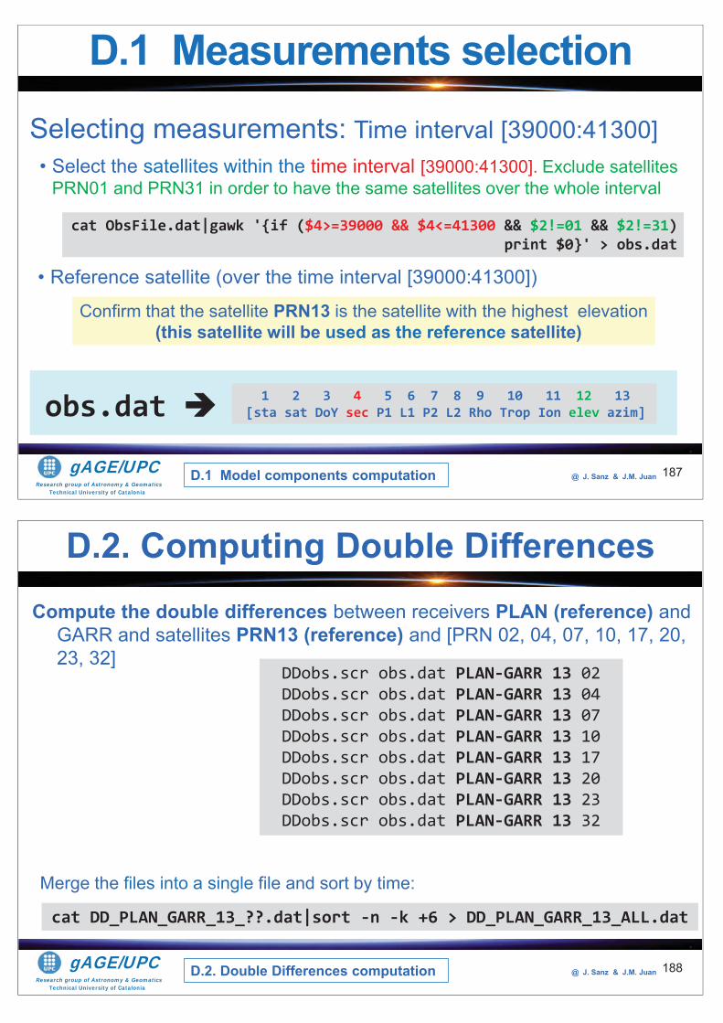
Research group of Astronomy & GeomaticsTechnical University of Catalonia
gAGE/UPC @ J. Sanz & J.M. Juan
• Select the satellites within the time interval [39000:41300]. Exclude satellites PRN01 and PRN31 in order to have the same satellites over the whole interval
187
D.1 Measurements selection
Confirm that the satellite PRN13 is the satellite with the highest elevation (this satellite will be used as the reference satellite)
cat ObsFile.dat|gawk '{if ($4>=39000 && $4<=41300 && $2!=01 && $2!=31) print $0}' > obs.dat
• Reference satellite (over the time interval [39000:41300])
Selecting measurements: Time interval [39000:41300]
1 2 3 4 5 6 7 8 9 10 11 12 13[sta sat DoY sec P1 L1 P2 L2 Rho Trop Ion elev azim]obs.dat
D.1 Model components computation
Research group of Astronomy & GeomaticsTechnical University of Catalonia
gAGE/UPC @ J. Sanz & J.M. Juan
Compute the double differences between receivers PLAN (reference) and GARR and satellites PRN13 (reference) and [PRN 02, 04, 07, 10, 17, 20, 23, 32]
188
DDobs.scr obs.dat PLAN-GARR 13 02DDobs.scr obs.dat PLAN-GARR 13 04DDobs.scr obs.dat PLAN-GARR 13 07DDobs.scr obs.dat PLAN-GARR 13 10DDobs.scr obs.dat PLAN-GARR 13 17DDobs.scr obs.dat PLAN-GARR 13 20DDobs.scr obs.dat PLAN-GARR 13 23DDobs.scr obs.dat PLAN-GARR 13 32
Merge the files into a single file and sort by time:
cat DD_PLAN_GARR_13_??.dat|sort -n -k +6 > DD_PLAN_GARR_13_ALL.dat
D.2. Double Differences computation
D.2. Computing Double Differences

Research group of Astronomy & GeomaticsTechnical University of Catalonia
gAGE/UPC @ J. Sanz & J.M. Juan 189
D.3.1 Using DDL1 carrier measurements, estimate the coordinates of receiver GARR taking PLAN as a reference receiver and correcting troposphere.
Consider only the two epochs used in the previous exercise: t1=39000 and t2=40500.
The following procedure can be applied:1. Compute the FLOATED solution, solving the equations system with
octave. Assess the accuracy of the floated solution.2. Apply the LAMBDA method to FIX the ambiguities. Compare the
results with the solution obtained by rounding the floated solution directly and by rounding the solution after decorrelation.
3. Repair the DDL1 carrier measurements with the DDN1 FIXED ambiguities and plot results to analyze the data.
4. Compute the FIXED solution.
D.3.1. Estimate GARR coordinates with DDL1 (using tropospheric corrections)
D.3. PLAN-GARR differential positioning with L1 carrier(using the computed differential corrections including troposphere)
Research group of Astronomy & GeomaticsTechnical University of Catalonia
gAGE/UPC @ J. Sanz & J.M. Juan 190
The script MakeL1DifTrpMat.scr builds the equations system
The OUTPUTare the files M1.dat and M2.dat associated with each epoch.
for the two epochs required t1=39000 and t2=40500, using the input file DD_PLAN_GARR_13_ALL.dat generated before.
[DDL1-DDRho-Trp]=[ Los_k- Los_13]*[dr] + [ A ]*[ 1*DDN1]
MakeL1DifTrpMat.scr DD_PLAN_GARR_13_ALL.dat 39000 40500
Execute:
Where: the columns of files M.dat are the vector y (first column) and Matrix G (next columns)
D.3. PLAN-GARR differential positioning with L1 carrier(using the computed differential corrections including troposphere)
D.3.1. Estimate GARR coordinates with DDL1 (using tropospheric corrections)
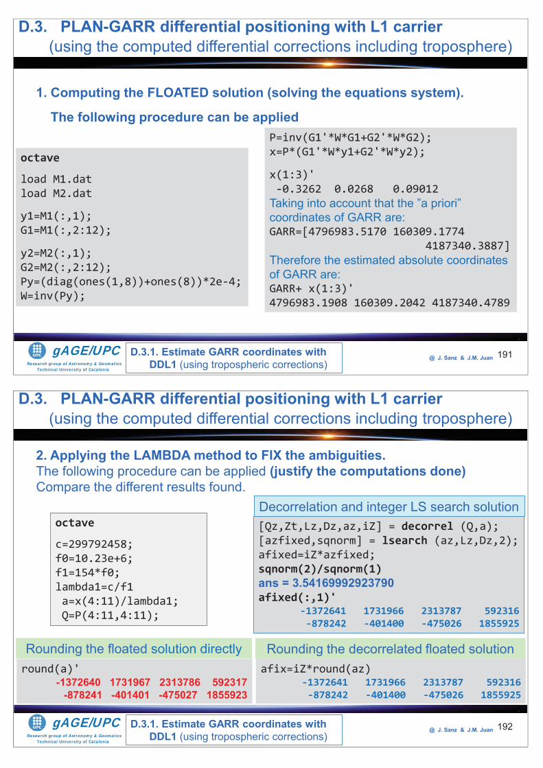
Research group of Astronomy & GeomaticsTechnical University of Catalonia
gAGE/UPC @ J. Sanz & J.M. Juan 191
1. Computing the FLOATED solution (solving the equations system).
The following procedure can be applied
octave
load M1.datload M2.dat
y1=M1(:,1);G1=M1(:,2:12);
y2=M2(:,1);G2=M2(:,2:12);Py=(diag(ones(1,8))+ones(8))*2e-4;W=inv(Py);
P=inv(G1'*W*G1+G2'*W*G2);x=P*(G1'*W*y1+G2'*W*y2);
x(1:3)'-0.3262 0.0268 0.09012
Taking into account that the ”a priori” coordinates of GARR are: GARR=[4796983.5170 160309.1774
4187340.3887]Therefore the estimated absolute coordinates of GARR are:GARR+ x(1:3)'4796983.1908 160309.2042 4187340.4789
D.3. PLAN-GARR differential positioning with L1 carrier(using the computed differential corrections including troposphere)
D.3.1. Estimate GARR coordinates with DDL1 (using tropospheric corrections)
Research group of Astronomy & GeomaticsTechnical University of Catalonia
gAGE/UPC @ J. Sanz & J.M. Juan 192
octave
c=299792458;f0=10.23e+6;f1=154*f0;lambda1=c/f1a=x(4:11)/lambda1;Q=P(4:11,4:11);
afix=iZ*round(az) -1372641 1731966 2313787 592316 -878242 -401400 -475026 1855925
[Qz,Zt,Lz,Dz,az,iZ] = decorrel (Q,a);[azfixed,sqnorm] = lsearch (az,Lz,Dz,2);afixed=iZ*azfixed;sqnorm(2)/sqnorm(1)ans = 3.54169992923790afixed(:,1)'
-1372641 1731966 2313787 592316 -878242 -401400 -475026 1855925
Rounding the decorrelated floated solutionround(a)'
-1372640 1731967 2313786 592317 -878241 -401401 -475027 1855923
Rounding the floated solution directly
Decorrelation and integer LS search solution
D.3. PLAN-GARR differential positioning with L1 carrier(using the computed differential corrections including troposphere)
D.3.1. Estimate GARR coordinates with DDL1 (using tropospheric corrections)
2. Applying the LAMBDA method to FIX the ambiguities. The following procedure can be applied (justify the computations done)Compare the different results found.
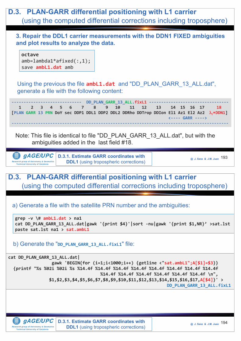
Research group of Astronomy & GeomaticsTechnical University of Catalonia
gAGE/UPC @ J. Sanz & J.M. Juan 193
3. Repair the DDL1 carrier measurements with the DDN1 FIXED ambiguities and plot results to analyze the data.
octaveamb=lambda1*afixed(:,1);save ambL1.dat amb
Using the previous the file ambL1.dat and "DD_PLAN_GARR_13_ALL.dat",generate a file with the following content:
----------------------------- DD_PLAN_GARR_13_ALL.fixL1 ---------------------------------1 2 3 4 5 6 7 8 9 10 11 12 13 14 15 16 17 18
[PLAN GARR 13 PRN DoY sec DDP1 DDL1 DDP2 DDL2 DDRho DDTrop DDIon El1 Az1 El2 Az2 DDN1]<---- GARR ---->
------------------------------------------------------------------------------------------
Note: This file is identical to file "DD_PLAN_GARR_13_ALL.dat", but with the ambiguities added in the last field #18.
D.3. PLAN-GARR differential positioning with L1 carrier(using the computed differential corrections including troposphere)
D.3.1. Estimate GARR coordinates with DDL1 (using tropospheric corrections)
Research group of Astronomy & GeomaticsTechnical University of Catalonia
gAGE/UPC @ J. Sanz & J.M. Juan 194
grep -v \# ambL1.dat > na1cat DD_PLAN_GARR_13_ALL.dat|gawk '{print $4}'|sort -nu|gawk '{print $1,NR}’ >sat.lstpaste sat.lst na1 > sat.ambL1
a) Generate a file with the satellite PRN number and the ambiguities:
cat DD_PLAN_GARR_13_ALL.dat|gawk 'BEGIN{for (i=1;i<1000;i++) {getline <"sat.ambL1";A[$1]=$3}}
{printf "%s %02i %02i %s %14.4f %14.4f %14.4f %14.4f %14.4f %14.4f %14.4f %14.4f %14.4f %14.4f %14.4f %14.4f %14.4f %14.4f \n",
$1,$2,$3,$4,$5,$6,$7,$8,$9,$10,$11,$12,$13,$14,$15,$16,$17,A[$4]}' > DD_PLAN_GARR_13_ALL.fixL1
b) Generate the "DD_PLAN_GARR_13_ALL.fixL1" file:
D.3. PLAN-GARR differential positioning with L1 carrier(using the computed differential corrections including troposphere)
D.3.1. Estimate GARR coordinates with DDL1 (using tropospheric corrections)
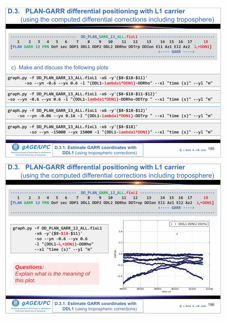
Research group of Astronomy & GeomaticsTechnical University of Catalonia
gAGE/UPC @ J. Sanz & J.M. Juan 195
graph.py -f DD_PLAN_GARR_13_ALL.fixL1 -x6 -y'($8-$18-$11)' -so --yn -0.6 --yx 0.6 -l "(DDL1-lambda1*DDN1)-DDRho" --xl "time (s)" --yl "m"
c) Make and discuss the following plots
----------------------------- DD_PLAN_GARR_13_ALL.fixL1 ---------------------------------1 2 3 4 5 6 7 8 9 10 11 12 13 14 15 16 17 18
[PLAN GARR 13 PRN DoY sec DDP1 DDL1 DDP2 DDL2 DDRho DDTrp DDIon El1 Az1 El2 Az2 DDN1]<---- GARR ---->
------------------------------------------------------------------------------------------
graph.py -f DD_PLAN_GARR_13_ALL.fixL1 -x6 -y'($8-$18-$11-$12)' -so --yn -0.6 --yx 0.6 -l "(DDL1-lambda1*DDN1)-DDRho-DDTrp " --xl "time (s)" --yl "m"
D.3. PLAN-GARR differential positioning with L1 carrier(using the computed differential corrections including troposphere)
D.3.1. Estimate GARR coordinates with DDL1 (using tropospheric corrections)
graph.py -f DD_PLAN_GARR_13_ALL.fixL1 -x6 -y'($8-$18-$12)' -so --yn -0.06 --yx 0.16 -l "(DDL1-lambda1*DDN1)-DDTrp " --xl "time (s)" --yl "m"
graph.py -f DD_PLAN_GARR_13_ALL.fixL1 -x6 -y'($8-$18)' -so --yn -15000 --yx 15000 -l "(DDL1-lambda1*DDN1)" --xl "time (s)" --yl "m"
Research group of Astronomy & GeomaticsTechnical University of Catalonia
gAGE/UPC @ J. Sanz & J.M. Juan 196
graph.py -f DD_PLAN_GARR_13_ALL.fixL1 -x6 -y'($8-$18-$11)' -so --yn -0.6 --yx 0.6 -l "(DDL1- DDN1)-DDRho" --xl "time (s)" --yl "m"
D.3. PLAN-GARR differential positioning with L1 carrier(using the computed differential corrections including troposphere)
D.3.1. Estimate GARR coordinates with DDL1 (using tropospheric corrections)
----------------------------- DD_PLAN_GARR_13_ALL.fixL1 ---------------------------------1 2 3 4 5 6 7 8 9 10 11 12 13 14 15 16 17 18
[PLAN GARR 13 PRN DoY sec DDP1 DDL1 DDP2 DDL2 DDRho DDTrop DDIon El1 Az1 El2 Az2 DDN1]<---- GARR ---->
------------------------------------------------------------------------------------------
Questions:Explain what is the meaning of this plot.
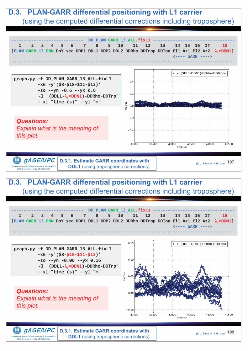
Research group of Astronomy & GeomaticsTechnical University of Catalonia
gAGE/UPC @ J. Sanz & J.M. Juan 197
graph.py -f DD_PLAN_GARR_13_ALL.fixL1 -x6 -y'($8-$18-$11-$12)' -so --yn -0.6 --yx 0.6 -l "(DDL1- DDN1)-DDRho-DDTrp"--xl "time (s)" --yl "m"
D.3. PLAN-GARR differential positioning with L1 carrier(using the computed differential corrections including troposphere)
D.3.1. Estimate GARR coordinates with DDL1 (using tropospheric corrections)
----------------------------- DD_PLAN_GARR_13_ALL.fixL1 ---------------------------------1 2 3 4 5 6 7 8 9 10 11 12 13 14 15 16 17 18
[PLAN GARR 13 PRN DoY sec DDP1 DDL1 DDP2 DDL2 DDRho DDTrop DDIon El1 Az1 El2 Az2 DDN1]<---- GARR ---->
------------------------------------------------------------------------------------------
Questions:Explain what is the meaning of this plot.
Research group of Astronomy & GeomaticsTechnical University of Catalonia
gAGE/UPC @ J. Sanz & J.M. Juan 198
graph.py -f DD_PLAN_GARR_13_ALL.fixL1 -x6 -y'($8-$18-$11-$12)' -so --yn -0.06 --yx 0.16 -l "(DDL1- DDN1)-DDRho-DDTrp"--xl "time (s)" --yl "m"
D.3. PLAN-GARR differential positioning with L1 carrier(using the computed differential corrections including troposphere)
D.3.1. Estimate GARR coordinates with DDL1 (using tropospheric corrections)
----------------------------- DD_PLAN_GARR_13_ALL.fixL1 ---------------------------------1 2 3 4 5 6 7 8 9 10 11 12 13 14 15 16 17 18
[PLAN GARR 13 PRN DoY sec DDP1 DDL1 DDP2 DDL2 DDRho DDTrop DDIon El1 Az1 El2 Az2 DDN1]<---- GARR ---->
------------------------------------------------------------------------------------------
Questions:Explain what is the meaning of this plot.
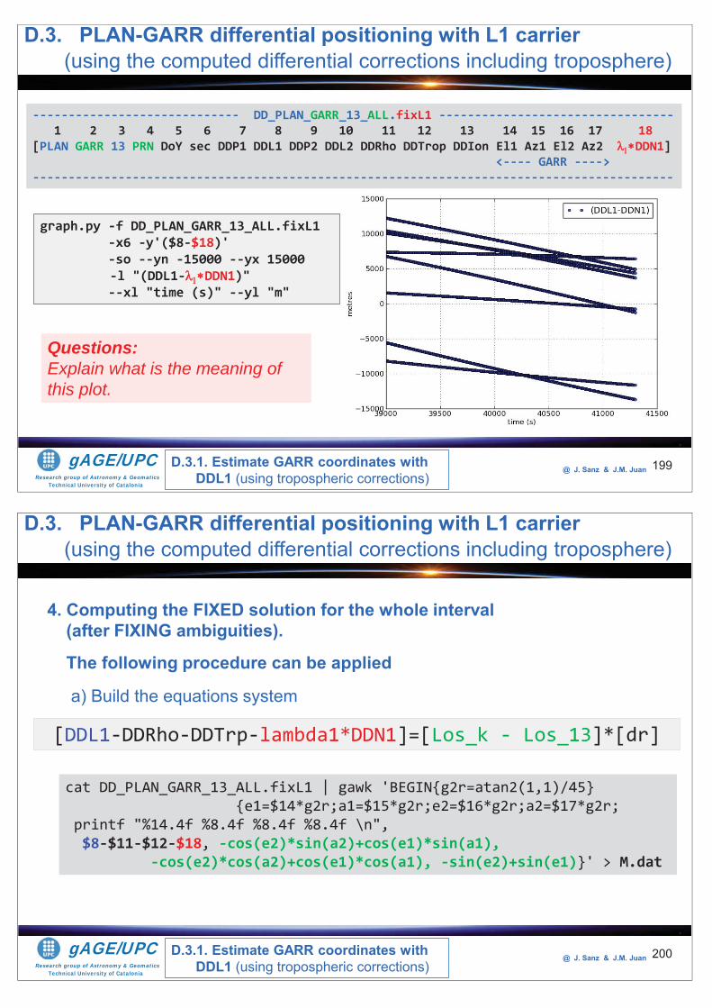
Research group of Astronomy & GeomaticsTechnical University of Catalonia
gAGE/UPC @ J. Sanz & J.M. Juan 199
graph.py -f DD_PLAN_GARR_13_ALL.fixL1 -x6 -y'($8-$18)' -so --yn -15000 --yx 15000 -l "(DDL1- DDN1)"--xl "time (s)" --yl "m"
D.3. PLAN-GARR differential positioning with L1 carrier(using the computed differential corrections including troposphere)
D.3.1. Estimate GARR coordinates with DDL1 (using tropospheric corrections)
----------------------------- DD_PLAN_GARR_13_ALL.fixL1 ---------------------------------1 2 3 4 5 6 7 8 9 10 11 12 13 14 15 16 17 18
[PLAN GARR 13 PRN DoY sec DDP1 DDL1 DDP2 DDL2 DDRho DDTrop DDIon El1 Az1 El2 Az2 DDN1]<---- GARR ---->
------------------------------------------------------------------------------------------
Questions:Explain what is the meaning of this plot.
Research group of Astronomy & GeomaticsTechnical University of Catalonia
gAGE/UPC @ J. Sanz & J.M. Juan 200
4. Computing the FIXED solution for the whole interval (after FIXING ambiguities).
The following procedure can be applied
a) Build the equations system
[DDL1-DDRho-DDTrp-lambda1*DDN1]=[Los_k - Los_13]*[dr]
cat DD_PLAN_GARR_13_ALL.fixL1 | gawk 'BEGIN{g2r=atan2(1,1)/45} {e1=$14*g2r;a1=$15*g2r;e2=$16*g2r;a2=$17*g2r;
printf "%14.4f %8.4f %8.4f %8.4f \n",$8-$11-$12-$18, -cos(e2)*sin(a2)+cos(e1)*sin(a1),
-cos(e2)*cos(a2)+cos(e1)*cos(a1), -sin(e2)+sin(e1)}' > M.dat
D.3. PLAN-GARR differential positioning with L1 carrier(using the computed differential corrections including troposphere)
D.3.1. Estimate GARR coordinates with DDL1 (using tropospheric corrections)
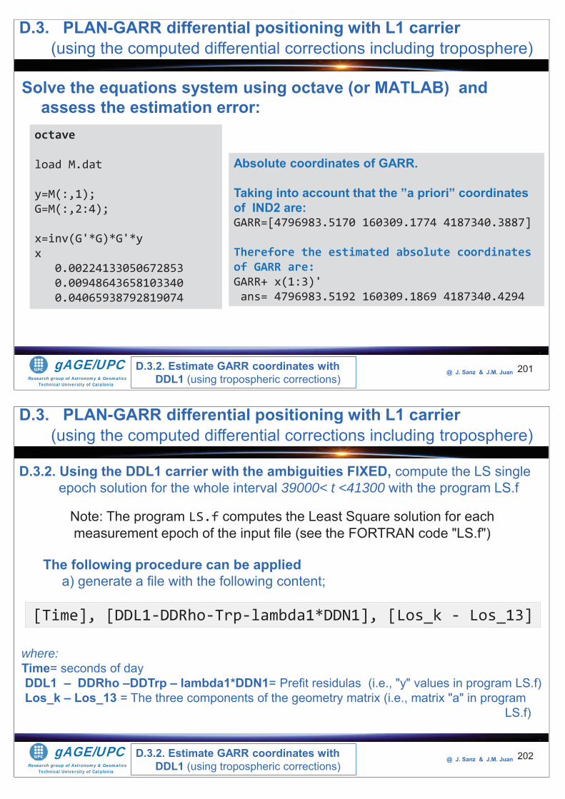
Research group of Astronomy & GeomaticsTechnical University of Catalonia
gAGE/UPC @ J. Sanz & J.M. Juan
Solve the equations system using octave (or MATLAB) and assess the estimation error:
201
octave
load M.dat
y=M(:,1);G=M(:,2:4);
x=inv(G'*G)*G'*yx
0.00224133050672853 0.00948643658103340 0.04065938792819074
Absolute coordinates of GARR.
Taking into account that the ”a priori” coordinates of IND2 are: GARR=[4796983.5170 160309.1774 4187340.3887]
Therefore the estimated absolute coordinates of GARR are:GARR+ x(1:3)'ans= 4796983.5192 160309.1869 4187340.4294
D.3. PLAN-GARR differential positioning with L1 carrier(using the computed differential corrections including troposphere)
D.3.2. Estimate GARR coordinates with DDL1 (using tropospheric corrections)
Research group of Astronomy & GeomaticsTechnical University of Catalonia
gAGE/UPC @ J. Sanz & J.M. Juan 202
D.3.2. Using the DDL1 carrier with the ambiguities FIXED, compute the LS single epoch solution for the whole interval 39000< t <41300 with the program LS.f
Note: The program LS.f computes the Least Square solution for eachmeasurement epoch of the input file (see the FORTRAN code "LS.f")
The following procedure can be applieda) generate a file with the following content;
[Time], [DDL1-DDRho-Trp-lambda1*DDN1], [Los_k - Los_13]
where:Time= seconds of day DDL1 – DDRho –DDTrp – lambda1*DDN1= Prefit residulas (i.e., "y" values in program LS.f)Los_k – Los_13 = The three components of the geometry matrix (i.e., matrix "a" in program
LS.f)
D.3. PLAN-GARR differential positioning with L1 carrier(using the computed differential corrections including troposphere)
D.3.2. Estimate GARR coordinates with DDL1 (using tropospheric corrections)
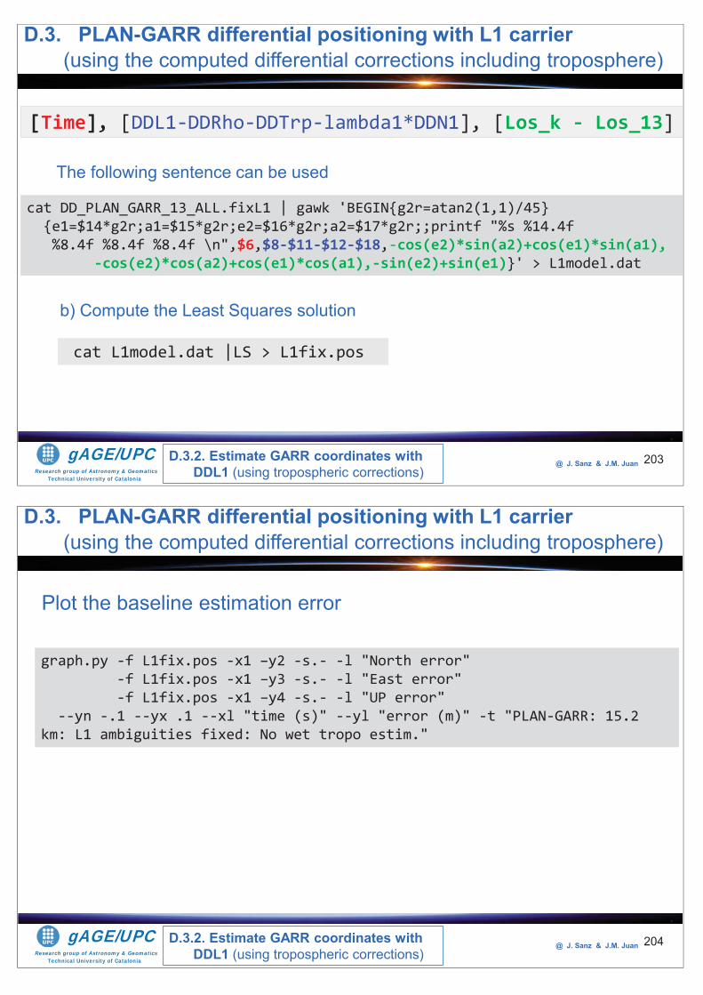
Research group of Astronomy & GeomaticsTechnical University of Catalonia
gAGE/UPC @ J. Sanz & J.M. Juan 203
The following sentence can be used
cat DD_PLAN_GARR_13_ALL.fixL1 | gawk 'BEGIN{g2r=atan2(1,1)/45} {e1=$14*g2r;a1=$15*g2r;e2=$16*g2r;a2=$17*g2r;;printf "%s %14.4f%8.4f %8.4f %8.4f \n",$6,$8-$11-$12-$18,-cos(e2)*sin(a2)+cos(e1)*sin(a1),
-cos(e2)*cos(a2)+cos(e1)*cos(a1),-sin(e2)+sin(e1)}' > L1model.dat
[Time], [DDL1-DDRho-DDTrp-lambda1*DDN1], [Los_k - Los_13]
b) Compute the Least Squares solution
cat L1model.dat |LS > L1fix.pos
D.3. PLAN-GARR differential positioning with L1 carrier(using the computed differential corrections including troposphere)
D.3.2. Estimate GARR coordinates with DDL1 (using tropospheric corrections)
Research group of Astronomy & GeomaticsTechnical University of Catalonia
gAGE/UPC @ J. Sanz & J.M. Juan 204
Plot the baseline estimation error
graph.py -f L1fix.pos -x1 –y2 -s.- -l "North error" -f L1fix.pos -x1 –y3 -s.- -l "East error" -f L1fix.pos -x1 –y4 -s.- -l "UP error"
--yn -.1 --yx .1 --xl "time (s)" --yl "error (m)" -t "PLAN-GARR: 15.2 km: L1 ambiguities fixed: No wet tropo estim."
D.3. PLAN-GARR differential positioning with L1 carrier(using the computed differential corrections including troposphere)
D.3.2. Estimate GARR coordinates with DDL1 (using tropospheric corrections)
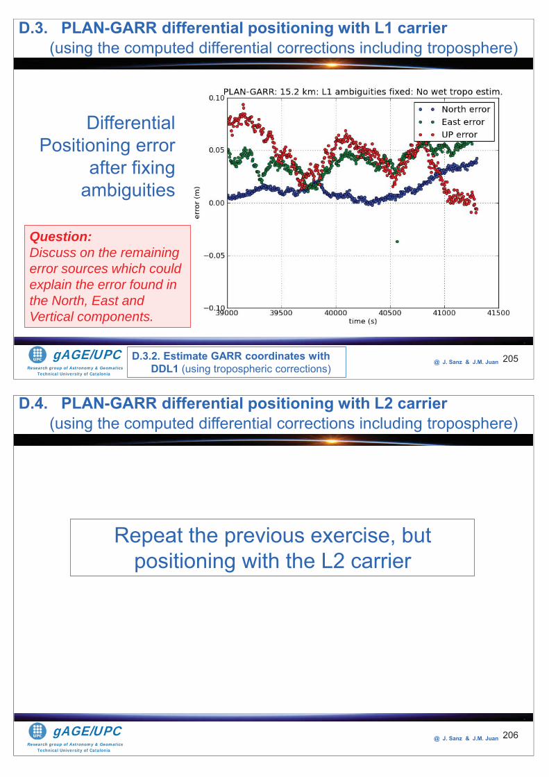
Research group of Astronomy & GeomaticsTechnical University of Catalonia
gAGE/UPC @ J. Sanz & J.M. Juan 205
Differential Positioning error
after fixing ambiguities
D.3. PLAN-GARR differential positioning with L1 carrier(using the computed differential corrections including troposphere)
D.3.2. Estimate GARR coordinates with DDL1 (using tropospheric corrections)
Question: Discuss on the remaining error sources which could explain the error found in the North, East and Vertical components.
Research group of Astronomy & GeomaticsTechnical University of Catalonia
gAGE/UPC @ J. Sanz & J.M. Juan 206
Repeat the previous exercise, but positioning with the L2 carrier
D.4. PLAN-GARR differential positioning with L2 carrier(using the computed differential corrections including troposphere)
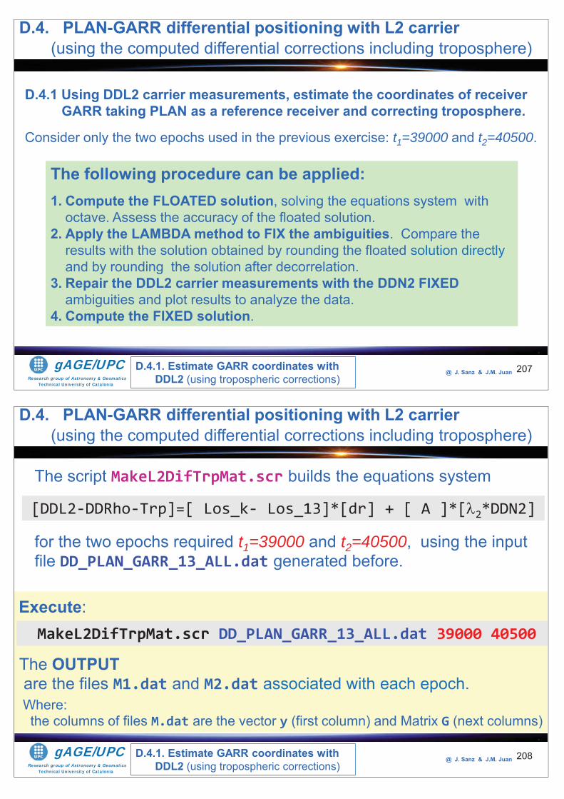
Research group of Astronomy & GeomaticsTechnical University of Catalonia
gAGE/UPC @ J. Sanz & J.M. Juan 207
D.4.1 Using DDL2 carrier measurements, estimate the coordinates of receiver GARR taking PLAN as a reference receiver and correcting troposphere.
Consider only the two epochs used in the previous exercise: t1=39000 and t2=40500.
The following procedure can be applied:1. Compute the FLOATED solution, solving the equations system with
octave. Assess the accuracy of the floated solution.2. Apply the LAMBDA method to FIX the ambiguities. Compare the
results with the solution obtained by rounding the floated solution directly and by rounding the solution after decorrelation.
3. Repair the DDL2 carrier measurements with the DDN2 FIXED ambiguities and plot results to analyze the data.
4. Compute the FIXED solution.
D.4.1. Estimate GARR coordinates with DDL2 (using tropospheric corrections)
D.4. PLAN-GARR differential positioning with L2 carrier(using the computed differential corrections including troposphere)
Research group of Astronomy & GeomaticsTechnical University of Catalonia
gAGE/UPC @ J. Sanz & J.M. Juan 208
The script MakeL2DifTrpMat.scr builds the equations system
The OUTPUTare the files M1.dat and M2.dat associated with each epoch.
for the two epochs required t1=39000 and t2=40500, using the input file DD_PLAN_GARR_13_ALL.dat generated before.
[DDL2-DDRho-Trp]=[ Los_k- Los_13]*[dr] + [ A ]*[ 2*DDN2]
MakeL2DifTrpMat.scr DD_PLAN_GARR_13_ALL.dat 39000 40500
Execute:
Where: the columns of files M.dat are the vector y (first column) and Matrix G (next columns)
D.4. PLAN-GARR differential positioning with L2 carrier(using the computed differential corrections including troposphere)
D.4.1. Estimate GARR coordinates with DDL2 (using tropospheric corrections)
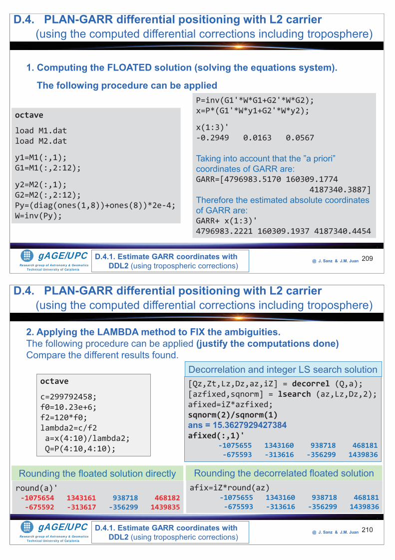
Research group of Astronomy & GeomaticsTechnical University of Catalonia
gAGE/UPC @ J. Sanz & J.M. Juan 209
1. Computing the FLOATED solution (solving the equations system).
The following procedure can be applied
octave
load M1.datload M2.dat
y1=M1(:,1);G1=M1(:,2:12);
y2=M2(:,1);G2=M2(:,2:12);Py=(diag(ones(1,8))+ones(8))*2e-4;W=inv(Py);
P=inv(G1'*W*G1+G2'*W*G2);x=P*(G1'*W*y1+G2'*W*y2);
x(1:3)'-0.2949 0.0163 0.0567
Taking into account that the ”a priori” coordinates of GARR are: GARR=[4796983.5170 160309.1774
4187340.3887]Therefore the estimated absolute coordinates of GARR are:GARR+ x(1:3)'4796983.2221 160309.1937 4187340.4454
D.4. PLAN-GARR differential positioning with L2 carrier(using the computed differential corrections including troposphere)
D.4.1. Estimate GARR coordinates with DDL2 (using tropospheric corrections)
Research group of Astronomy & GeomaticsTechnical University of Catalonia
gAGE/UPC @ J. Sanz & J.M. Juan 210
octave
c=299792458;f0=10.23e+6;f2=120*f0;lambda2=c/f2a=x(4:10)/lambda2;Q=P(4:10,4:10);
afix=iZ*round(az) -1075655 1343160 938718 468181 -675593 -313616 -356299 1439836
[Qz,Zt,Lz,Dz,az,iZ] = decorrel (Q,a);[azfixed,sqnorm] = lsearch (az,Lz,Dz,2);afixed=iZ*azfixed;sqnorm(2)/sqnorm(1)ans = 15.3627929427384afixed(:,1)'
-1075655 1343160 938718 468181 -675593 -313616 -356299 1439836
Rounding the decorrelated floated solutionround(a)' -1075654 1343161 938718 468182-675592 -313617 -356299 1439835
Rounding the floated solution directly
Decorrelation and integer LS search solution
D.4. PLAN-GARR differential positioning with L2 carrier(using the computed differential corrections including troposphere)
D.4.1. Estimate GARR coordinates with DDL2 (using tropospheric corrections)
2. Applying the LAMBDA method to FIX the ambiguities. The following procedure can be applied (justify the computations done)Compare the different results found.
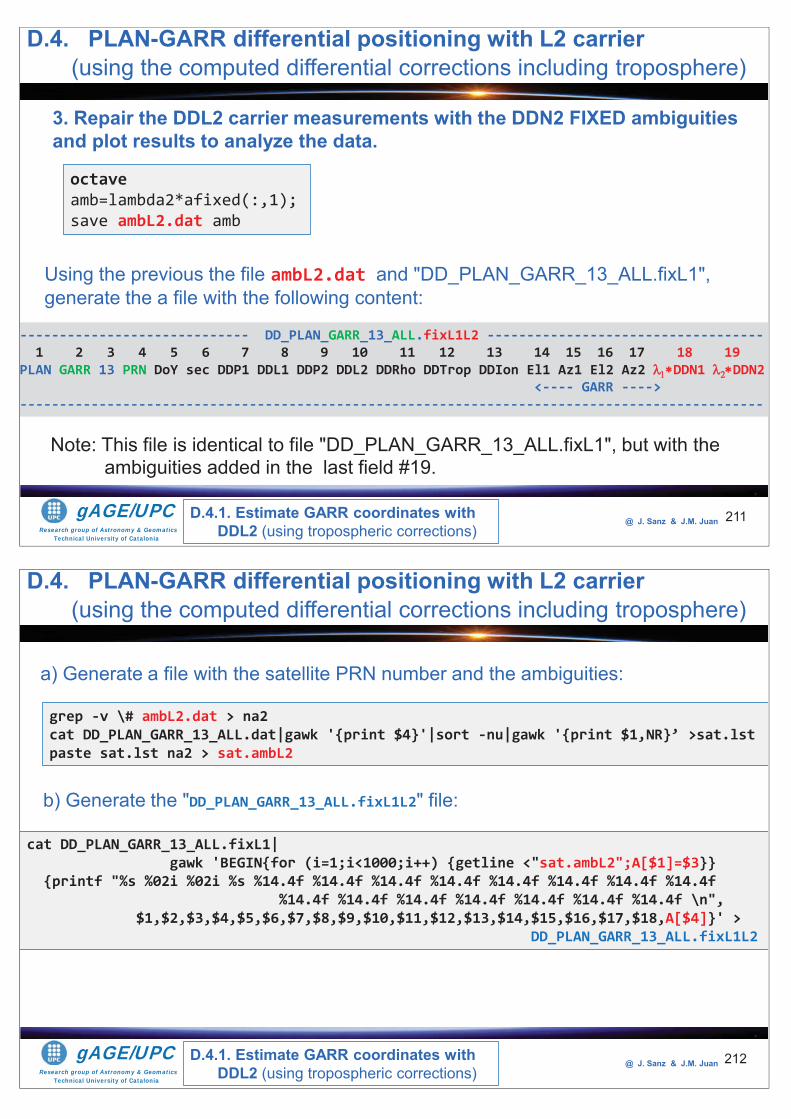
Research group of Astronomy & GeomaticsTechnical University of Catalonia
gAGE/UPC @ J. Sanz & J.M. Juan 211
3. Repair the DDL2 carrier measurements with the DDN2 FIXED ambiguities and plot results to analyze the data.
octaveamb=lambda2*afixed(:,1);save ambL2.dat amb
Using the previous the file ambL2.dat and "DD_PLAN_GARR_13_ALL.fixL1",generate the a file with the following content:
----------------------------- DD_PLAN_GARR_13_ALL.fixL1L2 -----------------------------------1 2 3 4 5 6 7 8 9 10 11 12 13 14 15 16 17 18 19
PLAN GARR 13 PRN DoY sec DDP1 DDL1 DDP2 DDL2 DDRho DDTrop DDIon El1 Az1 El2 Az2 DDN1 DDN2<---- GARR ---->
----------------------------------------------------------------------------------------------
Note: This file is identical to file "DD_PLAN_GARR_13_ALL.fixL1", but with the ambiguities added in the last field #19.
D.4. PLAN-GARR differential positioning with L2 carrier(using the computed differential corrections including troposphere)
D.4.1. Estimate GARR coordinates with DDL2 (using tropospheric corrections)
Research group of Astronomy & GeomaticsTechnical University of Catalonia
gAGE/UPC @ J. Sanz & J.M. Juan 212
grep -v \# ambL2.dat > na2cat DD_PLAN_GARR_13_ALL.dat|gawk '{print $4}'|sort -nu|gawk '{print $1,NR}’ >sat.lstpaste sat.lst na2 > sat.ambL2
a) Generate a file with the satellite PRN number and the ambiguities:
cat DD_PLAN_GARR_13_ALL.fixL1|gawk 'BEGIN{for (i=1;i<1000;i++) {getline <"sat.ambL2";A[$1]=$3}}
{printf "%s %02i %02i %s %14.4f %14.4f %14.4f %14.4f %14.4f %14.4f %14.4f %14.4f %14.4f %14.4f %14.4f %14.4f %14.4f %14.4f %14.4f \n",
$1,$2,$3,$4,$5,$6,$7,$8,$9,$10,$11,$12,$13,$14,$15,$16,$17,$18,A[$4]}' >DD_PLAN_GARR_13_ALL.fixL1L2
b) Generate the "DD_PLAN_GARR_13_ALL.fixL1L2" file:
D.4. PLAN-GARR differential positioning with L2 carrier(using the computed differential corrections including troposphere)
D.4.1. Estimate GARR coordinates with DDL2 (using tropospheric corrections)
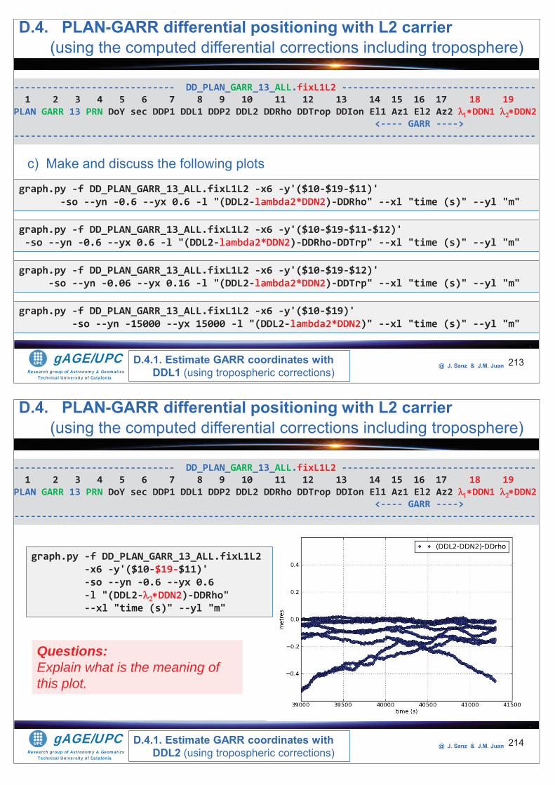
Research group of Astronomy & GeomaticsTechnical University of Catalonia
gAGE/UPC @ J. Sanz & J.M. Juan 213
graph.py -f DD_PLAN_GARR_13_ALL.fixL1L2 -x6 -y'($10-$19-$11)' -so --yn -0.6 --yx 0.6 -l "(DDL2-lambda2*DDN2)-DDRho" --xl "time (s)" --yl "m"
c) Make and discuss the following plots
graph.py -f DD_PLAN_GARR_13_ALL.fixL1L2 -x6 -y'($10-$19-$11-$12)' -so --yn -0.6 --yx 0.6 -l "(DDL2-lambda2*DDN2)-DDRho-DDTrp" --xl "time (s)" --yl "m"
D.4. PLAN-GARR differential positioning with L2 carrier(using the computed differential corrections including troposphere)
D.4.1. Estimate GARR coordinates with DDL1 (using tropospheric corrections)
graph.py -f DD_PLAN_GARR_13_ALL.fixL1L2 -x6 -y'($10-$19-$12)' -so --yn -0.06 --yx 0.16 -l "(DDL2-lambda2*DDN2)-DDTrp" --xl "time (s)" --yl "m"
----------------------------- DD_PLAN_GARR_13_ALL.fixL1L2 -----------------------------------1 2 3 4 5 6 7 8 9 10 11 12 13 14 15 16 17 18 19
PLAN GARR 13 PRN DoY sec DDP1 DDL1 DDP2 DDL2 DDRho DDTrop DDIon El1 Az1 El2 Az2 DDN1 DDN2<---- GARR ---->
----------------------------------------------------------------------------------------------
graph.py -f DD_PLAN_GARR_13_ALL.fixL1L2 -x6 -y'($10-$19)' -so --yn -15000 --yx 15000 -l "(DDL2-lambda2*DDN2)" --xl "time (s)" --yl "m"
Research group of Astronomy & GeomaticsTechnical University of Catalonia
gAGE/UPC @ J. Sanz & J.M. Juan 214
graph.py -f DD_PLAN_GARR_13_ALL.fixL1L2 -x6 -y'($10-$19-$11)' -so --yn -0.6 --yx 0.6 -l "(DDL2- DDN2)-DDRho" --xl "time (s)" --yl "m"
D.4. PLAN-GARR differential positioning with L2 carrier(using the computed differential corrections including troposphere)
D.4.1. Estimate GARR coordinates with DDL2 (using tropospheric corrections)
----------------------------- DD_PLAN_GARR_13_ALL.fixL1L2 -----------------------------------1 2 3 4 5 6 7 8 9 10 11 12 13 14 15 16 17 18 19
PLAN GARR 13 PRN DoY sec DDP1 DDL1 DDP2 DDL2 DDRho DDTrop DDIon El1 Az1 El2 Az2 DDN1 DDN2<---- GARR ---->
----------------------------------------------------------------------------------------------
Questions:Explain what is the meaning of this plot.
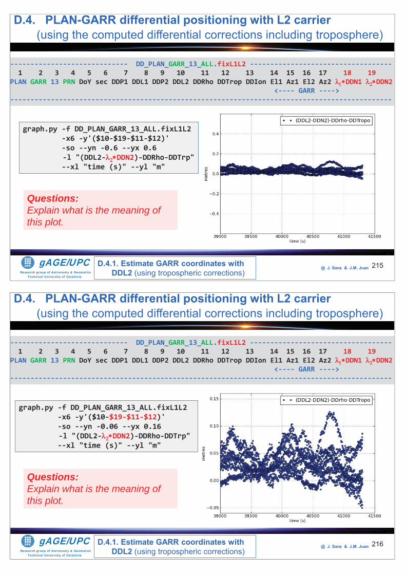
Research group of Astronomy & GeomaticsTechnical University of Catalonia
gAGE/UPC @ J. Sanz & J.M. Juan 215
graph.py -f DD_PLAN_GARR_13_ALL.fixL1L2 -x6 -y'($10-$19-$11-$12)' -so --yn -0.6 --yx 0.6 -l "(DDL2- DDN2)-DDRho-DDTrp"--xl "time (s)" --yl "m"
D.4. PLAN-GARR differential positioning with L2 carrier(using the computed differential corrections including troposphere)
D.4.1. Estimate GARR coordinates with DDL2 (using tropospheric corrections)
----------------------------- DD_PLAN_GARR_13_ALL.fixL1L2 -----------------------------------1 2 3 4 5 6 7 8 9 10 11 12 13 14 15 16 17 18 19
PLAN GARR 13 PRN DoY sec DDP1 DDL1 DDP2 DDL2 DDRho DDTrop DDIon El1 Az1 El2 Az2 DDN1 DDN2<---- GARR ---->
----------------------------------------------------------------------------------------------
Questions:Explain what is the meaning of this plot.
Research group of Astronomy & GeomaticsTechnical University of Catalonia
gAGE/UPC @ J. Sanz & J.M. Juan 216
graph.py -f DD_PLAN_GARR_13_ALL.fixL1L2 -x6 -y'($10-$19-$11-$12)' -so --yn -0.06 --yx 0.16 -l "(DDL2- DDN2)-DDRho-DDTrp"--xl "time (s)" --yl "m"
D.4. PLAN-GARR differential positioning with L2 carrier(using the computed differential corrections including troposphere)
D.4.1. Estimate GARR coordinates with DDL2 (using tropospheric corrections)
----------------------------- DD_PLAN_GARR_13_ALL.fixL1L2 -----------------------------------1 2 3 4 5 6 7 8 9 10 11 12 13 14 15 16 17 18 19
PLAN GARR 13 PRN DoY sec DDP1 DDL1 DDP2 DDL2 DDRho DDTrop DDIon El1 Az1 El2 Az2 DDN1 DDN2<---- GARR ---->
----------------------------------------------------------------------------------------------
Questions:Explain what is the meaning of this plot.
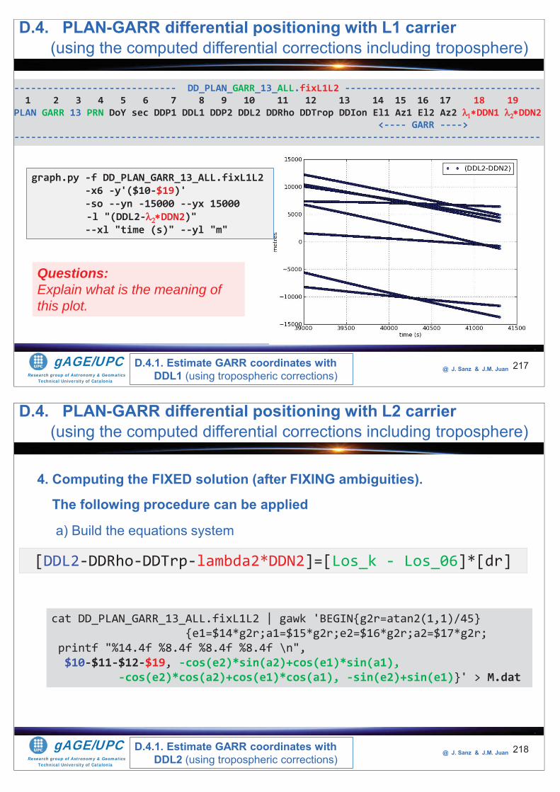
Research group of Astronomy & GeomaticsTechnical University of Catalonia
gAGE/UPC @ J. Sanz & J.M. Juan 217
graph.py -f DD_PLAN_GARR_13_ALL.fixL1L2 -x6 -y'($10-$19)' -so --yn -15000 --yx 15000 -l "(DDL2- DDN2)"--xl "time (s)" --yl "m"
D.4. PLAN-GARR differential positioning with L1 carrier(using the computed differential corrections including troposphere)
D.4.1. Estimate GARR coordinates with DDL1 (using tropospheric corrections)
----------------------------- DD_PLAN_GARR_13_ALL.fixL1L2 -----------------------------------1 2 3 4 5 6 7 8 9 10 11 12 13 14 15 16 17 18 19
PLAN GARR 13 PRN DoY sec DDP1 DDL1 DDP2 DDL2 DDRho DDTrop DDIon El1 Az1 El2 Az2 DDN1 DDN2<---- GARR ---->
----------------------------------------------------------------------------------------------
Questions:Explain what is the meaning of this plot.
Research group of Astronomy & GeomaticsTechnical University of Catalonia
gAGE/UPC @ J. Sanz & J.M. Juan 218
4. Computing the FIXED solution (after FIXING ambiguities).
The following procedure can be applied
a) Build the equations system
[DDL2-DDRho-DDTrp-lambda2*DDN2]=[Los_k - Los_06]*[dr]
cat DD_PLAN_GARR_13_ALL.fixL1L2 | gawk 'BEGIN{g2r=atan2(1,1)/45} {e1=$14*g2r;a1=$15*g2r;e2=$16*g2r;a2=$17*g2r;
printf "%14.4f %8.4f %8.4f %8.4f \n",$10-$11-$12-$19, -cos(e2)*sin(a2)+cos(e1)*sin(a1),
-cos(e2)*cos(a2)+cos(e1)*cos(a1), -sin(e2)+sin(e1)}' > M.dat
D.4. PLAN-GARR differential positioning with L2 carrier(using the computed differential corrections including troposphere)
D.4.1. Estimate GARR coordinates with DDL2 (using tropospheric corrections)
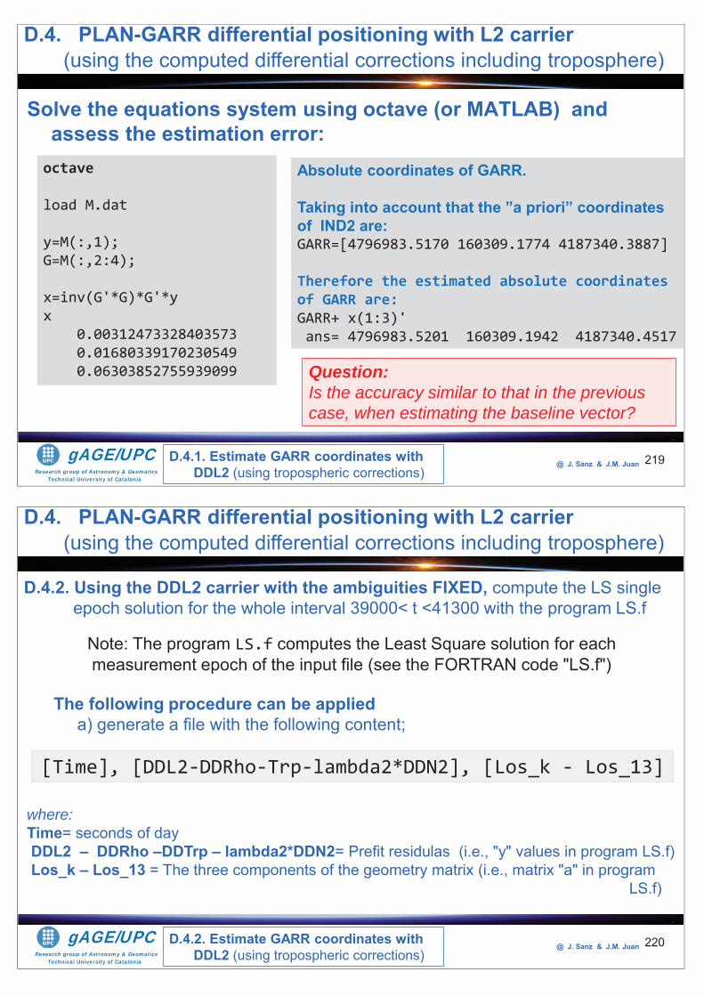
Research group of Astronomy & GeomaticsTechnical University of Catalonia
gAGE/UPC @ J. Sanz & J.M. Juan
Solve the equations system using octave (or MATLAB) and assess the estimation error:
219
octave
load M.dat
y=M(:,1);G=M(:,2:4);
x=inv(G'*G)*G'*yx
0.00312473328403573 0.01680339170230549 0.06303852755939099
Absolute coordinates of GARR.
Taking into account that the ”a priori” coordinates of IND2 are: GARR=[4796983.5170 160309.1774 4187340.3887]
Therefore the estimated absolute coordinates of GARR are:GARR+ x(1:3)'ans= 4796983.5201 160309.1942 4187340.4517
Question: Is the accuracy similar to that in the previous case, when estimating the baseline vector?
D.4. PLAN-GARR differential positioning with L2 carrier(using the computed differential corrections including troposphere)
D.4.1. Estimate GARR coordinates with DDL2 (using tropospheric corrections)
Research group of Astronomy & GeomaticsTechnical University of Catalonia
gAGE/UPC @ J. Sanz & J.M. Juan 220
D.4.2. Using the DDL2 carrier with the ambiguities FIXED, compute the LS single epoch solution for the whole interval 39000< t <41300 with the program LS.f
Note: The program LS.f computes the Least Square solution for eachmeasurement epoch of the input file (see the FORTRAN code "LS.f")
The following procedure can be applieda) generate a file with the following content;
[Time], [DDL2-DDRho-Trp-lambda2*DDN2], [Los_k - Los_13]
where:Time= seconds of day DDL2 – DDRho –DDTrp – lambda2*DDN2= Prefit residulas (i.e., "y" values in program LS.f)Los_k – Los_13 = The three components of the geometry matrix (i.e., matrix "a" in program
LS.f)
D.4. PLAN-GARR differential positioning with L2 carrier(using the computed differential corrections including troposphere)
D.4.2. Estimate GARR coordinates with DDL2 (using tropospheric corrections)
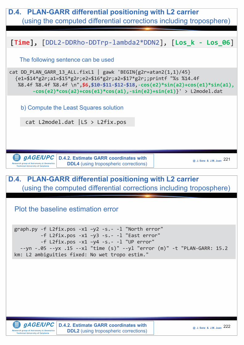
Research group of Astronomy & GeomaticsTechnical University of Catalonia
gAGE/UPC @ J. Sanz & J.M. Juan 221
The following sentence can be used
cat DD_PLAN_GARR_13_ALL.fixL1 | gawk 'BEGIN{g2r=atan2(1,1)/45} {e1=$14*g2r;a1=$15*g2r;e2=$16*g2r;a2=$17*g2r;;printf "%s %14.4f%8.4f %8.4f %8.4f \n",$6,$10-$11-$12-$18,-cos(e2)*sin(a2)+cos(e1)*sin(a1),
-cos(e2)*cos(a2)+cos(e1)*cos(a1),-sin(e2)+sin(e1)}' > L2model.dat
[Time], [DDL2-DDRho-DDTrp-lambda2*DDN2], [Los_k - Los_06]
b) Compute the Least Squares solution
cat L2model.dat |LS > L2fix.pos
D.4. PLAN-GARR differential positioning with L2 carrier(using the computed differential corrections including troposphere)
D.4.2. Estimate GARR coordinates with DDL4 (using tropospheric corrections)
Research group of Astronomy & GeomaticsTechnical University of Catalonia
gAGE/UPC @ J. Sanz & J.M. Juan 222
Plot the baseline estimation error
graph.py -f L2fix.pos -x1 –y2 -s.- -l "North error" -f L2fix.pos -x1 –y3 -s.- -l "East error" -f L2fix.pos -x1 –y4 -s.- -l "UP error"
--yn -.05 --yx .15 --xl "time (s)" --yl "error (m)" -t "PLAN-GARR: 15.2 km: L2 ambiguities fixed: No wet tropo estim."
D.4. PLAN-GARR differential positioning with L2 carrier(using the computed differential corrections including troposphere)
D.4.2. Estimate GARR coordinates with DDL2 (using tropospheric corrections)
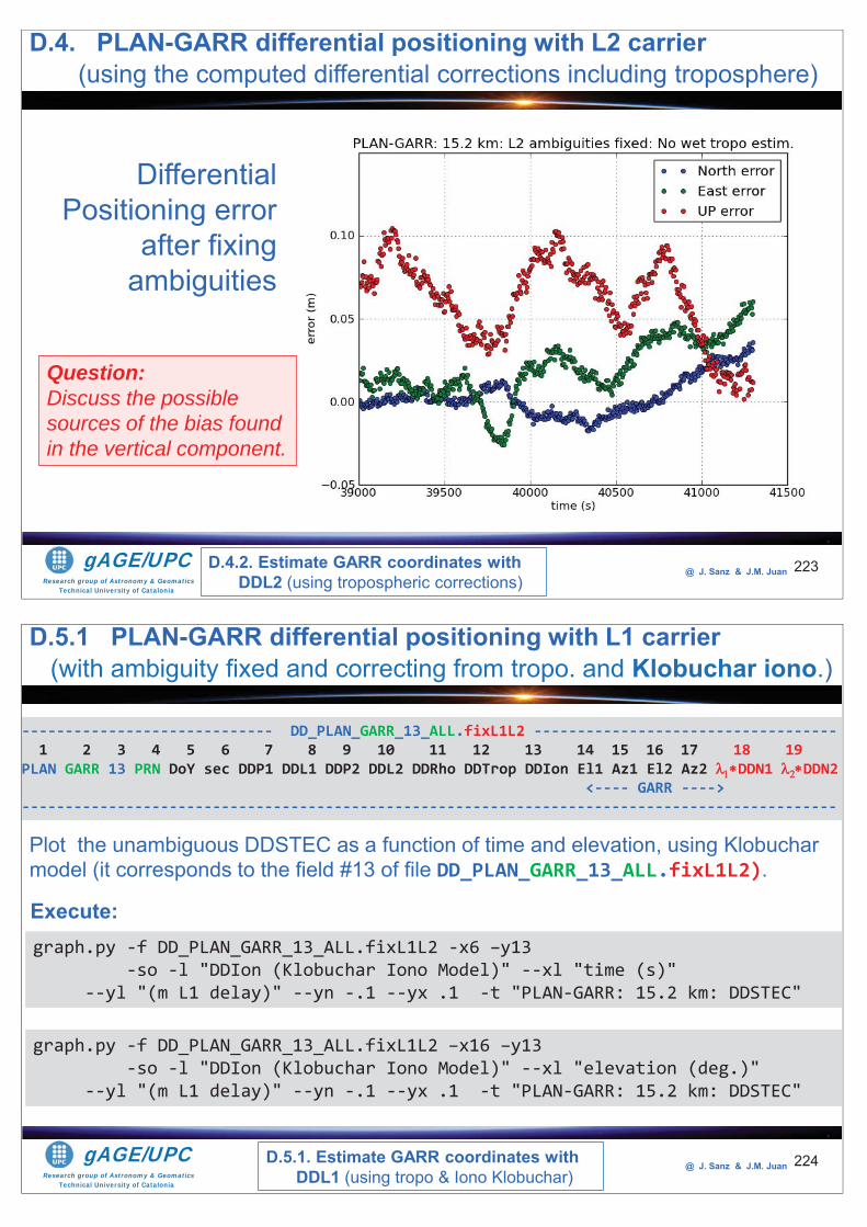
Research group of Astronomy & GeomaticsTechnical University of Catalonia
gAGE/UPC @ J. Sanz & J.M. Juan 223
Differential Positioning error
after fixing ambiguities
D.4. PLAN-GARR differential positioning with L2 carrier(using the computed differential corrections including troposphere)
D.4.2. Estimate GARR coordinates with DDL2 (using tropospheric corrections)
Question: Discuss the possible sources of the bias found in the vertical component.
Research group of Astronomy & GeomaticsTechnical University of Catalonia
gAGE/UPC @ J. Sanz & J.M. Juan 224
Plot the unambiguous DDSTEC as a function of time and elevation, using Klobucharmodel (it corresponds to the field #13 of file DD_PLAN_GARR_13_ALL.fixL1L2).
graph.py -f DD_PLAN_GARR_13_ALL.fixL1L2 -x6 –y13 -so -l "DDIon (Klobuchar Iono Model)" --xl "time (s)"
--yl "(m L1 delay)" --yn -.1 --yx .1 -t "PLAN-GARR: 15.2 km: DDSTEC"
----------------------------- DD_PLAN_GARR_13_ALL.fixL1L2 -----------------------------------1 2 3 4 5 6 7 8 9 10 11 12 13 14 15 16 17 18 19
PLAN GARR 13 PRN DoY sec DDP1 DDL1 DDP2 DDL2 DDRho DDTrop DDIon El1 Az1 El2 Az2 DDN1 DDN2<---- GARR ---->
----------------------------------------------------------------------------------------------
graph.py -f DD_PLAN_GARR_13_ALL.fixL1L2 –x16 –y13-so -l "DDIon (Klobuchar Iono Model)" --xl "elevation (deg.)"
--yl "(m L1 delay)" --yn -.1 --yx .1 -t "PLAN-GARR: 15.2 km: DDSTEC"
Execute:
D.5.1 PLAN-GARR differential positioning with L1 carrier(with ambiguity fixed and correcting from tropo. and Klobuchar iono.)
D.5.1. Estimate GARR coordinates with DDL1 (using tropo & Iono Klobuchar)
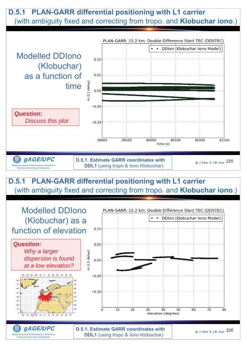
Research group of Astronomy & GeomaticsTechnical University of Catalonia
gAGE/UPC @ J. Sanz & J.M. Juan 225
Modelled DDIono(Klobuchar)
as a function of time
Question: Discuss this plot
D.5.1 PLAN-GARR differential positioning with L1 carrier(with ambiguity fixed and correcting from tropo. and Klobuchar iono.)
D.5.1. Estimate GARR coordinates with DDL1 (using tropo & Iono Klobuchar)
Research group of Astronomy & GeomaticsTechnical University of Catalonia
gAGE/UPC @ J. Sanz & J.M. Juan 226
Modelled DDIono(Klobuchar) as a
function of elevationQuestion:
Why a larger dispersion is found at a low elevation?
D.5.1 PLAN-GARR differential positioning with L1 carrier(with ambiguity fixed and correcting from tropo. and Klobuchar iono.)
D.5.1. Estimate GARR coordinates with DDL1 (using tropo & Iono Klobuchar)
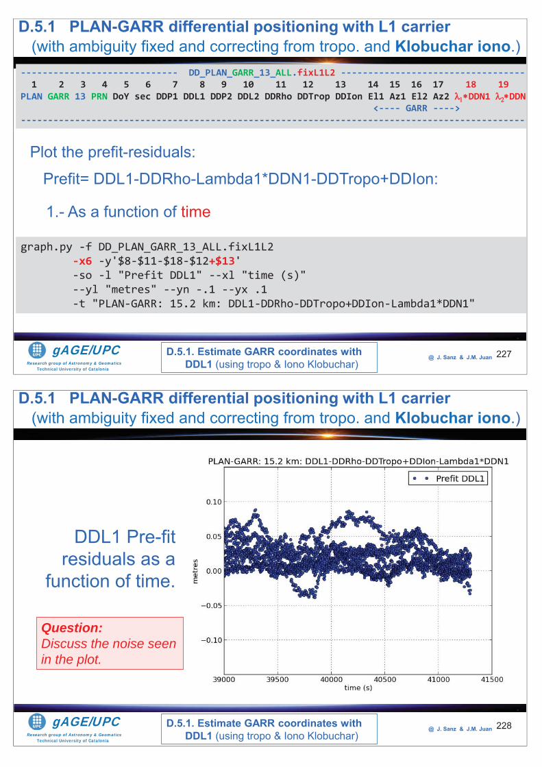
Research group of Astronomy & GeomaticsTechnical University of Catalonia
gAGE/UPC @ J. Sanz & J.M. Juan 227
Plot the prefit-residuals:Prefit= DDL1-DDRho-Lambda1*DDN1-DDTropo+DDIon:
graph.py -f DD_PLAN_GARR_13_ALL.fixL1L2 -x6 -y'$8-$11-$18-$12+$13' -so -l "Prefit DDL1" --xl "time (s)" --yl "metres" --yn -.1 --yx .1 -t "PLAN-GARR: 15.2 km: DDL1-DDRho-DDTropo+DDIon-Lambda1*DDN1"
----------------------------- DD_PLAN_GARR_13_ALL.fixL1L2 -----------------------------------1 2 3 4 5 6 7 8 9 10 11 12 13 14 15 16 17 18 19
PLAN GARR 13 PRN DoY sec DDP1 DDL1 DDP2 DDL2 DDRho DDTrop DDIon El1 Az1 El2 Az2 DDN1 DDN2<---- GARR ---->
----------------------------------------------------------------------------------------------
1.- As a function of time
D.5.1 PLAN-GARR differential positioning with L1 carrier(with ambiguity fixed and correcting from tropo. and Klobuchar iono.)
D.5.1. Estimate GARR coordinates with DDL1 (using tropo & Iono Klobuchar)
Research group of Astronomy & GeomaticsTechnical University of Catalonia
gAGE/UPC @ J. Sanz & J.M. Juan 228
DDL1 Pre-fit residuals as a
function of time.
Question: Discuss the noise seen in the plot.
D.5.1 PLAN-GARR differential positioning with L1 carrier(with ambiguity fixed and correcting from tropo. and Klobuchar iono.)
D.5.1. Estimate GARR coordinates with DDL1 (using tropo & Iono Klobuchar)
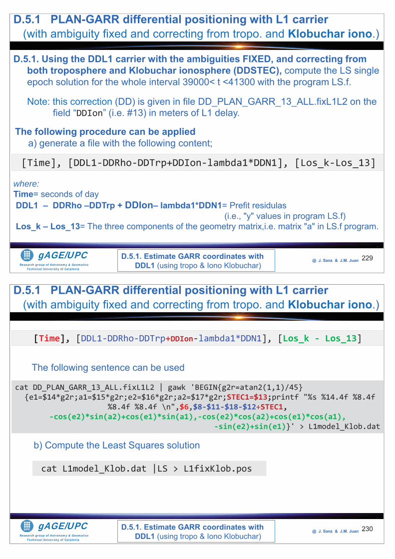
Research group of Astronomy & GeomaticsTechnical University of Catalonia
gAGE/UPC @ J. Sanz & J.M. Juan 229
The following procedure can be applieda) generate a file with the following content;
[Time], [DDL1-DDRho-DDTrp+DDIon-lambda1*DDN1], [Los_k-Los_13]
where:Time= seconds of dayDDL1 – DDRho –DDTrp + DDIon– lambda1*DDN1= Prefit residulas
(i.e., "y" values in program LS.f)Los_k – Los_13= The three components of the geometry matrix,i.e. matrix "a" in LS.f program.
D.5.1. Estimate GARR coordinates with DDL1 (using tropo & Iono Klobuchar)
D.5.1 PLAN-GARR differential positioning with L1 carrier(with ambiguity fixed and correcting from tropo. and Klobuchar iono.)
D.5.1. Using the DDL1 carrier with the ambiguities FIXED, and correcting from both troposphere and Klobuchar ionosphere (DDSTEC), compute the LS single epoch solution for the whole interval 39000< t <41300 with the program LS.f.
Note: this correction (DD) is given in file DD_PLAN_GARR_13_ALL.fixL1L2 on thefield “DDIon” (i.e. #13) in meters of L1 delay.
Research group of Astronomy & GeomaticsTechnical University of Catalonia
gAGE/UPC @ J. Sanz & J.M. Juan 230
The following sentence can be used
cat DD_PLAN_GARR_13_ALL.fixL1L2 | gawk 'BEGIN{g2r=atan2(1,1)/45}{e1=$14*g2r;a1=$15*g2r;e2=$16*g2r;a2=$17*g2r;STEC1=$13;printf "%s %14.4f %8.4f
%8.4f %8.4f \n",$6,$8-$11-$18-$12+STEC1,-cos(e2)*sin(a2)+cos(e1)*sin(a1),-cos(e2)*cos(a2)+cos(e1)*cos(a1),
-sin(e2)+sin(e1)}' > L1model_Klob.dat
[Time], [DDL1-DDRho-DDTrp+DDIon-lambda1*DDN1], [Los_k - Los_13]
b) Compute the Least Squares solution
cat L1model_Klob.dat |LS > L1fixKlob.pos
D.5.1. Estimate GARR coordinates with DDL1 (using tropo & Iono Klobuchar)
D.5.1 PLAN-GARR differential positioning with L1 carrier(with ambiguity fixed and correcting from tropo. and Klobuchar iono.)
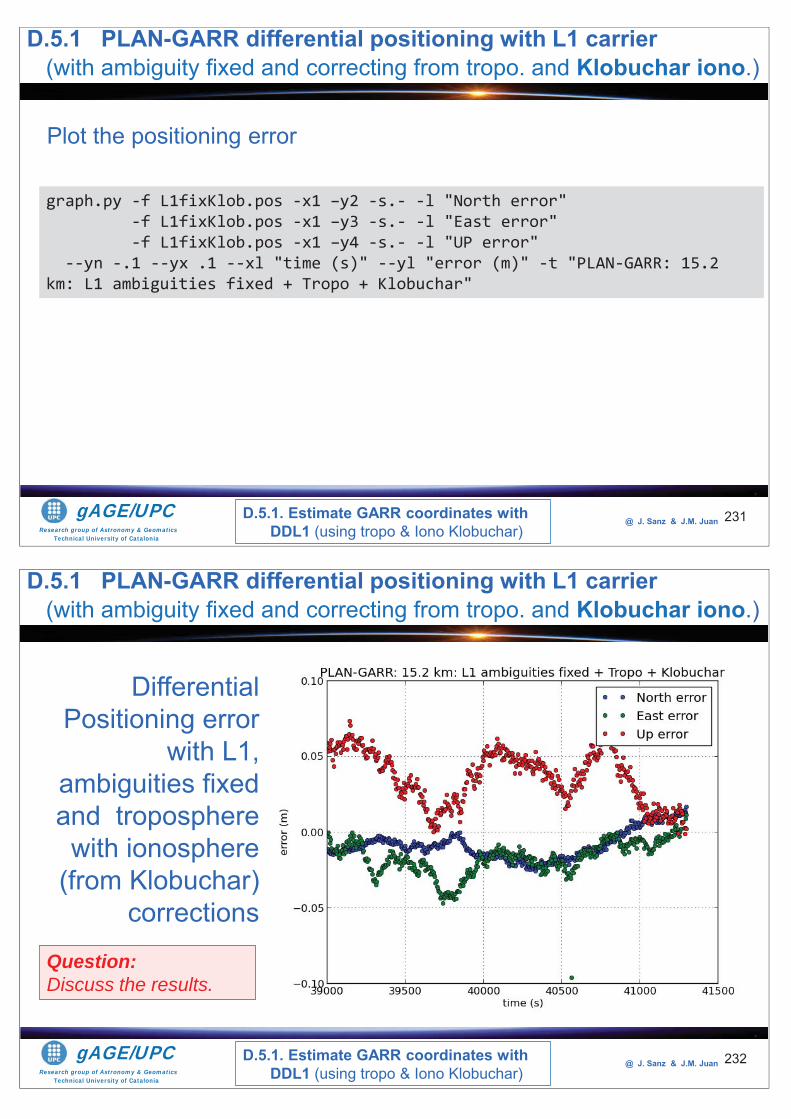
Research group of Astronomy & GeomaticsTechnical University of Catalonia
gAGE/UPC @ J. Sanz & J.M. Juan 231
Plot the positioning error
graph.py -f L1fixKlob.pos -x1 –y2 -s.- -l "North error" -f L1fixKlob.pos -x1 –y3 -s.- -l "East error" -f L1fixKlob.pos -x1 –y4 -s.- -l "UP error"
--yn -.1 --yx .1 --xl "time (s)" --yl "error (m)" -t "PLAN-GARR: 15.2 km: L1 ambiguities fixed + Tropo + Klobuchar"
D.5.1. Estimate GARR coordinates with DDL1 (using tropo & Iono Klobuchar)
D.5.1 PLAN-GARR differential positioning with L1 carrier(with ambiguity fixed and correcting from tropo. and Klobuchar iono.)
Research group of Astronomy & GeomaticsTechnical University of Catalonia
gAGE/UPC @ J. Sanz & J.M. Juan 232
Differential Positioning error
with L1, ambiguities fixed and troposphere
with ionosphere (from Klobuchar)
corrections
Question: Discuss the results.
D.5.1. Estimate GARR coordinates with DDL1 (using tropo & Iono Klobuchar)
D.5.1 PLAN-GARR differential positioning with L1 carrier(with ambiguity fixed and correcting from tropo. and Klobuchar iono.)
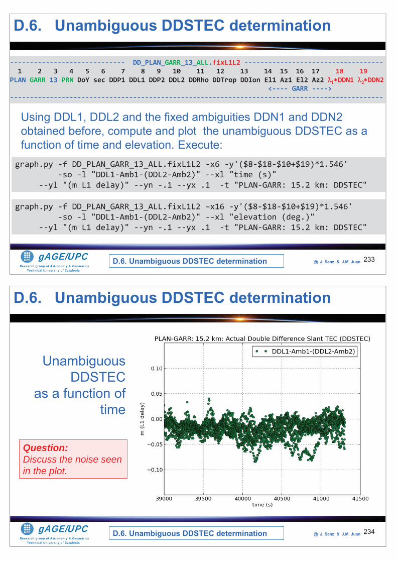
Research group of Astronomy & GeomaticsTechnical University of Catalonia
gAGE/UPC @ J. Sanz & J.M. Juan 233
D.6. Unambiguous DDSTEC determination
D.6. Unambiguous DDSTEC determination
Using DDL1, DDL2 and the fixed ambiguities DDN1 and DDN2 obtained before, compute and plot the unambiguous DDSTEC as a function of time and elevation. Execute:
graph.py -f DD_PLAN_GARR_13_ALL.fixL1L2 -x6 -y'($8-$18-$10+$19)*1.546' -so -l "DDL1-Amb1-(DDL2-Amb2)" --xl "time (s)"
--yl "(m L1 delay)" --yn -.1 --yx .1 -t "PLAN-GARR: 15.2 km: DDSTEC"
----------------------------- DD_PLAN_GARR_13_ALL.fixL1L2 -----------------------------------1 2 3 4 5 6 7 8 9 10 11 12 13 14 15 16 17 18 19
PLAN GARR 13 PRN DoY sec DDP1 DDL1 DDP2 DDL2 DDRho DDTrop DDIon El1 Az1 El2 Az2 DDN1 DDN2<---- GARR ---->
----------------------------------------------------------------------------------------------
graph.py -f DD_PLAN_GARR_13_ALL.fixL1L2 –x16 -y'($8-$18-$10+$19)*1.546' -so -l "DDL1-Amb1-(DDL2-Amb2)" --xl "elevation (deg.)"
--yl "(m L1 delay)" --yn -.1 --yx .1 -t "PLAN-GARR: 15.2 km: DDSTEC"
Research group of Astronomy & GeomaticsTechnical University of Catalonia
gAGE/UPC @ J. Sanz & J.M. Juan 234
Unambiguous DDSTEC
as a function of time
Question: Discuss the noise seen in the plot.
D.6. Unambiguous DDSTEC determination
D.6. Unambiguous DDSTEC determination
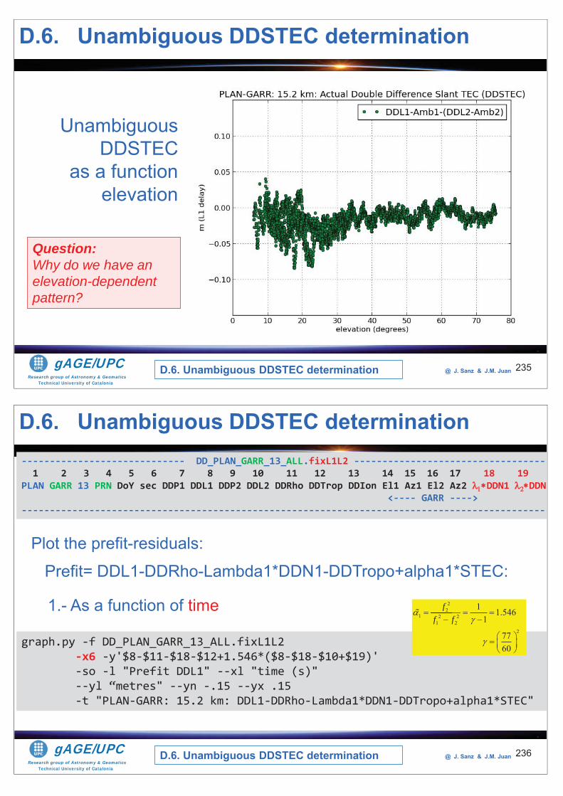
Research group of Astronomy & GeomaticsTechnical University of Catalonia
gAGE/UPC @ J. Sanz & J.M. Juan 235
Unambiguous DDSTEC
as a function elevation
Question: Why do we have an elevation-dependent pattern?
D.6. Unambiguous DDSTEC determination
D.6. Unambiguous DDSTEC determination
Research group of Astronomy & GeomaticsTechnical University of Catalonia
gAGE/UPC @ J. Sanz & J.M. Juan 236
Plot the prefit-residuals:Prefit= DDL1-DDRho-Lambda1*DDN1-DDTropo+alpha1*STEC:
graph.py -f DD_PLAN_GARR_13_ALL.fixL1L2 -x6 -y'$8-$11-$18-$12+1.546*($8-$18-$10+$19)' -so -l "Prefit DDL1" --xl "time (s)" --yl “metres" --yn -.15 --yx .15 -t "PLAN-GARR: 15.2 km: DDL1-DDRho-Lambda1*DDN1-DDTropo+alpha1*STEC"
----------------------------- DD_PLAN_GARR_13_ALL.fixL1L2 -----------------------------------1 2 3 4 5 6 7 8 9 10 11 12 13 14 15 16 17 18 19
PLAN GARR 13 PRN DoY sec DDP1 DDL1 DDP2 DDL2 DDRho DDTrop DDIon El1 Az1 El2 Az2 DDN1 DDN2<---- GARR ---->
----------------------------------------------------------------------------------------------
1.- As a function of time
D.6. Unambiguous DDSTEC determination
D.6. Unambiguous DDSTEC determination
22
1 2 21 2
2
1 1.5461
7760
ff f
21 2
f2
f 2
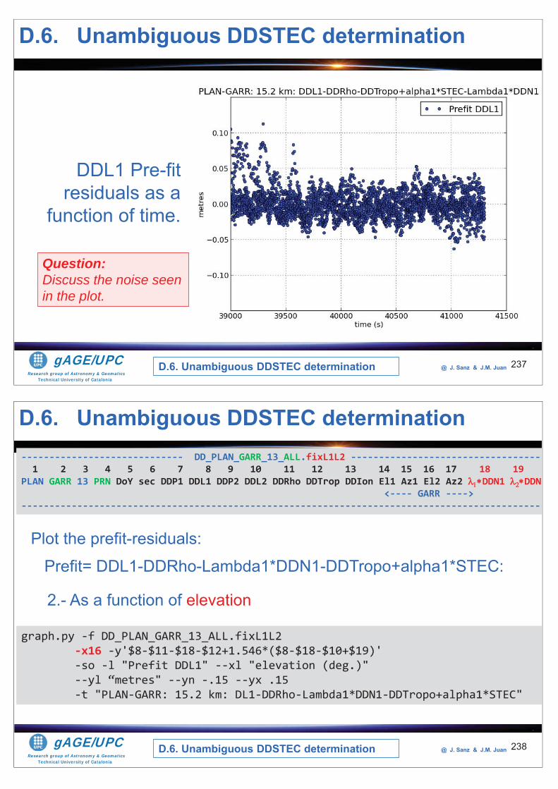
Research group of Astronomy & GeomaticsTechnical University of Catalonia
gAGE/UPC @ J. Sanz & J.M. Juan 237
DDL1 Pre-fit residuals as a
function of time.
Question: Discuss the noise seen in the plot.
D.6. Unambiguous DDSTEC determination
D.6. Unambiguous DDSTEC determination
Research group of Astronomy & GeomaticsTechnical University of Catalonia
gAGE/UPC @ J. Sanz & J.M. Juan 238
graph.py -f DD_PLAN_GARR_13_ALL.fixL1L2 -x16 -y'$8-$11-$18-$12+1.546*($8-$18-$10+$19)' -so -l "Prefit DDL1" --xl "elevation (deg.)" --yl “metres" --yn -.15 --yx .15 -t "PLAN-GARR: 15.2 km: DL1-DDRho-Lambda1*DDN1-DDTropo+alpha1*STEC"
----------------------------- DD_PLAN_GARR_13_ALL.fixL1L2 -----------------------------------1 2 3 4 5 6 7 8 9 10 11 12 13 14 15 16 17 18 19
PLAN GARR 13 PRN DoY sec DDP1 DDL1 DDP2 DDL2 DDRho DDTrop DDIon El1 Az1 El2 Az2 DDN1 DDN2<---- GARR ---->
----------------------------------------------------------------------------------------------
2.- As a function of elevation
Plot the prefit-residuals:Prefit= DDL1-DDRho-Lambda1*DDN1-DDTropo+alpha1*STEC:
D.6. Unambiguous DDSTEC determination
D.6. Unambiguous DDSTEC determination
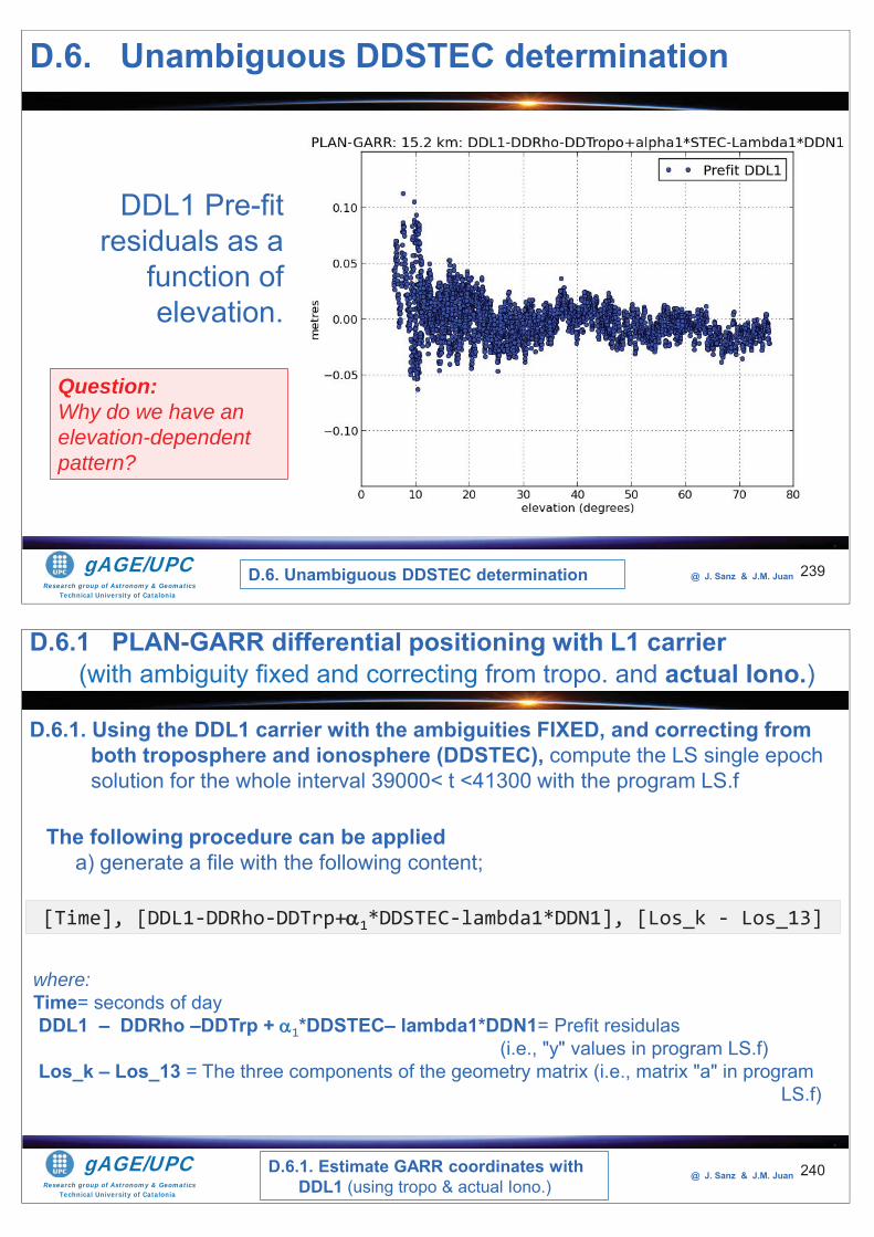
Research group of Astronomy & GeomaticsTechnical University of Catalonia
gAGE/UPC @ J. Sanz & J.M. Juan 239
DDL1 Pre-fit residuals as a
function of elevation.
Question: Why do we have an elevation-dependent pattern?
D.6. Unambiguous DDSTEC determination
D.6. Unambiguous DDSTEC determination
Research group of Astronomy & GeomaticsTechnical University of Catalonia
gAGE/UPC @ J. Sanz & J.M. Juan 240
D.6.1. Using the DDL1 carrier with the ambiguities FIXED, and correcting from both troposphere and ionosphere (DDSTEC), compute the LS single epoch solution for the whole interval 39000< t <41300 with the program LS.f
The following procedure can be applieda) generate a file with the following content;
[Time], [DDL1-DDRho-DDTrp+ 1*DDSTEC-lambda1*DDN1], [Los_k - Los_13]
where:Time= seconds of dayDDL1 – DDRho –DDTrp + 1*DDSTEC– lambda1*DDN1= Prefit residulas
(i.e., "y" values in program LS.f)Los_k – Los_13 = The three components of the geometry matrix (i.e., matrix "a" in program
LS.f)
D.6.1 PLAN-GARR differential positioning with L1 carrier(with ambiguity fixed and correcting from tropo. and actual Iono.)
D.6.1. Estimate GARR coordinates with DDL1 (using tropo & actual Iono.)
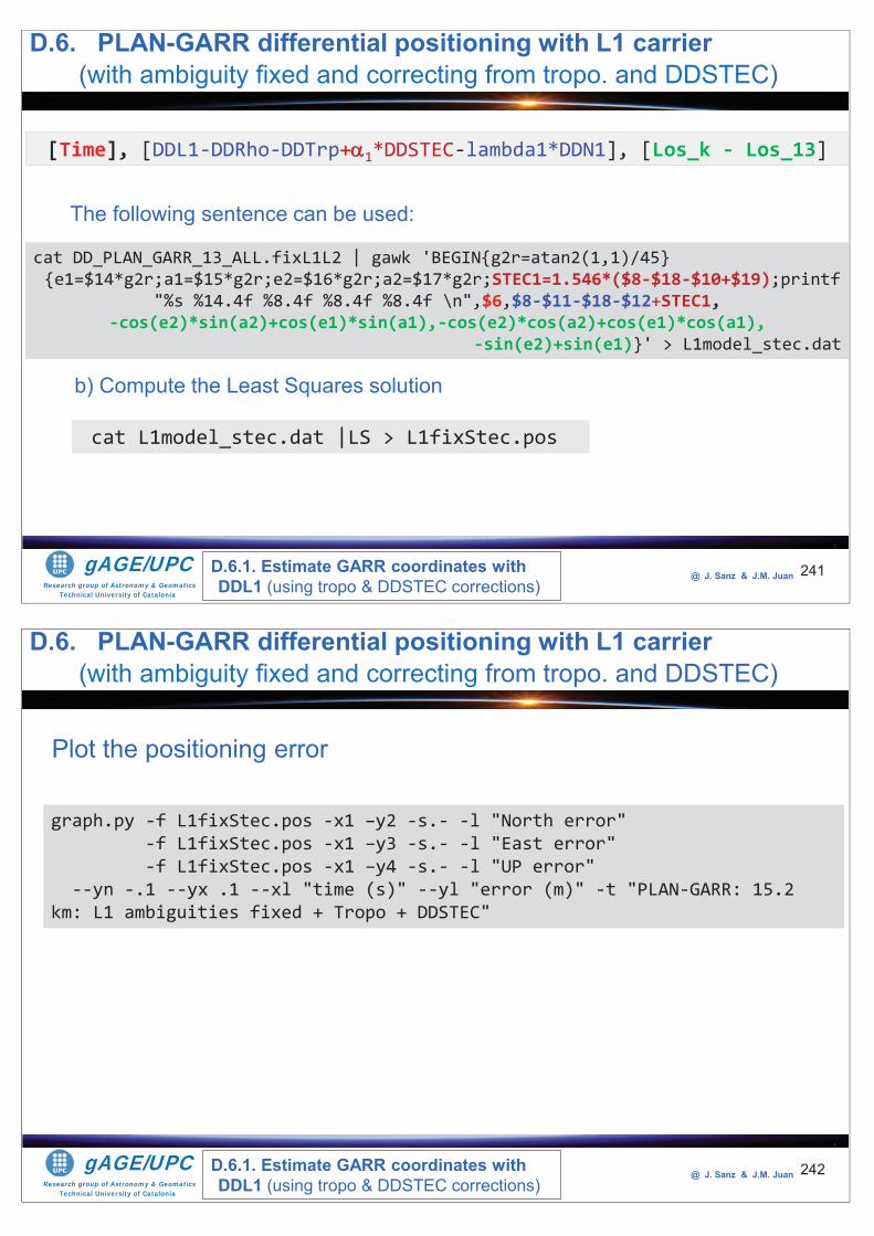
Research group of Astronomy & GeomaticsTechnical University of Catalonia
gAGE/UPC @ J. Sanz & J.M. Juan 241
The following sentence can be used:
cat DD_PLAN_GARR_13_ALL.fixL1L2 | gawk 'BEGIN{g2r=atan2(1,1)/45}{e1=$14*g2r;a1=$15*g2r;e2=$16*g2r;a2=$17*g2r;STEC1=1.546*($8-$18-$10+$19);printf
"%s %14.4f %8.4f %8.4f %8.4f \n",$6,$8-$11-$18-$12+STEC1,-cos(e2)*sin(a2)+cos(e1)*sin(a1),-cos(e2)*cos(a2)+cos(e1)*cos(a1),
-sin(e2)+sin(e1)}' > L1model_stec.dat
[Time], [DDL1-DDRho-DDTrp+ 1*DDSTEC-lambda1*DDN1], [Los_k - Los_13]
b) Compute the Least Squares solution
cat L1model_stec.dat |LS > L1fixStec.pos
D.6. PLAN-GARR differential positioning with L1 carrier(with ambiguity fixed and correcting from tropo. and DDSTEC)
D.6.1. Estimate GARR coordinates with DDL1 (using tropo & DDSTEC corrections)
Research group of Astronomy & GeomaticsTechnical University of Catalonia
gAGE/UPC @ J. Sanz & J.M. Juan 242
Plot the positioning error
graph.py -f L1fixStec.pos -x1 –y2 -s.- -l "North error" -f L1fixStec.pos -x1 –y3 -s.- -l "East error" -f L1fixStec.pos -x1 –y4 -s.- -l "UP error"
--yn -.1 --yx .1 --xl "time (s)" --yl "error (m)" -t "PLAN-GARR: 15.2 km: L1 ambiguities fixed + Tropo + DDSTEC"
D.6. PLAN-GARR differential positioning with L1 carrier(with ambiguity fixed and correcting from tropo. and DDSTEC)
D.6.1. Estimate GARR coordinates with DDL1 (using tropo & DDSTEC corrections)
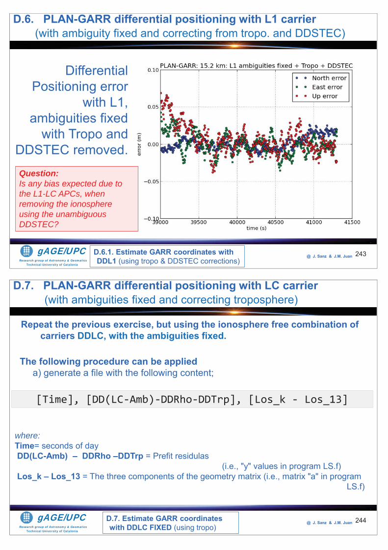
Research group of Astronomy & GeomaticsTechnical University of Catalonia
gAGE/UPC @ J. Sanz & J.M. Juan 243
Differential Positioning error
with L1, ambiguities fixed
with Tropo and DDSTEC removed.Question: Is any bias expected due to the L1-LC APCs, when removing the ionosphere using the unambiguous DDSTEC?
D.6. PLAN-GARR differential positioning with L1 carrier(with ambiguity fixed and correcting from tropo. and DDSTEC)
D.6.1. Estimate GARR coordinates with DDL1 (using tropo & DDSTEC corrections)
Research group of Astronomy & GeomaticsTechnical University of Catalonia
gAGE/UPC @ J. Sanz & J.M. Juan 244
Repeat the previous exercise, but using the ionosphere free combination of carriers DDLC, with the ambiguities fixed.
The following procedure can be applieda) generate a file with the following content;
[Time], [DD(LC-Amb)-DDRho-DDTrp], [Los_k - Los_13]
where:Time= seconds of day DD(LC-Amb) – DDRho –DDTrp = Prefit residulas
(i.e., "y" values in program LS.f)Los_k – Los_13 = The three components of the geometry matrix (i.e., matrix "a" in program
LS.f)
D.7. PLAN-GARR differential positioning with LC carrier(with ambiguities fixed and correcting troposphere)
D.7. Estimate GARR coordinates with DDLC FIXED (using tropo)
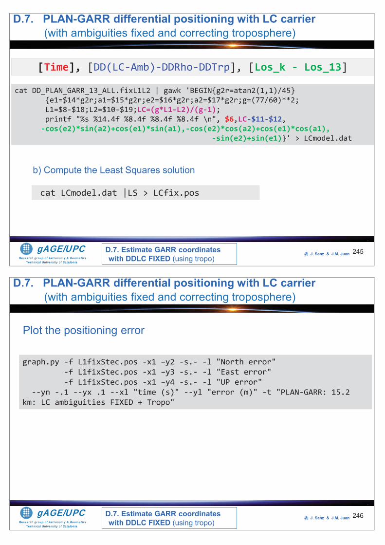
Research group of Astronomy & GeomaticsTechnical University of Catalonia
gAGE/UPC @ J. Sanz & J.M. Juan 245
The following sentence can be used:cat DD_PLAN_GARR_13_ALL.fixL1L2 | gawk 'BEGIN{g2r=atan2(1,1)/45} {e1=$14*g2r;a1=$15*g2r;e2=$16*g2r;a2=$17*g2r;g=(77/60)**2;L1=$8-$18;L2=$10-$19;LC=(g*L1-L2)/(g-1);printf "%s %14.4f %8.4f %8.4f %8.4f \n", $6,LC-$11-$12,-cos(e2)*sin(a2)+cos(e1)*sin(a1),-cos(e2)*cos(a2)+cos(e1)*cos(a1),
-sin(e2)+sin(e1)}' > LCmodel.dat
[Time], [DD(LC-Amb)-DDRho-DDTrp], [Los_k - Los_13]
b) Compute the Least Squares solution
cat LCmodel.dat |LS > LCfix.pos
D.7. Estimate GARR coordinates with DDLC FIXED (using tropo)
D.7. PLAN-GARR differential positioning with LC carrier(with ambiguities fixed and correcting troposphere)
Research group of Astronomy & GeomaticsTechnical University of Catalonia
gAGE/UPC @ J. Sanz & J.M. Juan 246
Plot the positioning error
graph.py -f L1fixStec.pos -x1 –y2 -s.- -l "North error" -f L1fixStec.pos -x1 –y3 -s.- -l "East error" -f L1fixStec.pos -x1 –y4 -s.- -l "UP error"
--yn -.1 --yx .1 --xl "time (s)" --yl "error (m)" -t "PLAN-GARR: 15.2 km: LC ambiguities FIXED + Tropo"
D.7. Estimate GARR coordinates with DDLC FIXED (using tropo)
D.7. PLAN-GARR differential positioning with LC carrier(with ambiguities fixed and correcting troposphere)
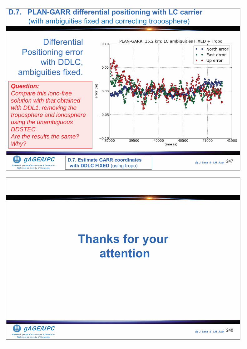
Research group of Astronomy & GeomaticsTechnical University of Catalonia
gAGE/UPC @ J. Sanz & J.M. Juan 247
Differential Positioning error
with DDLC, ambiguities fixed.
Question: Compare this iono-free solution with that obtained with DDL1, removing the troposphere and ionosphere using the unambiguous DDSTEC. Are the results the same? Why?
D.7. PLAN-GARR differential positioning with LC carrier(with ambiguities fixed and correcting troposphere)
D.7. Estimate GARR coordinates with DDLC FIXED (using tropo)
Research group of Astronomy & GeomaticsTechnical University of Catalonia
gAGE/UPC @ J. Sanz & J.M. Juan 248
Thanks for yourattention

Research group of Astronomy & GeomaticsTechnical University of Catalonia
gAGE/UPC @ J. Sanz & J.M. Juan
• To the University of Delft for the MATLAB files of LAMBDA method.• To the INDRA company and Institut Cartogràfic de Catalunya for the
data files of receivers IND1,IND2, IND2 and PLAN, GARR, respectively.• To Adrià Rovira-Garcia for his contribution to the editing of this material
and gLAB updating and integrating this learning material into the GLUE.
The ESA/UPC GNSS-Lab Tool suite (gLAB) has been developed under theESA Education Office contract N. P1081434.
Acknowledgements

List of Acronyms
List of Acronyms
AGW Atmospheric Gravity Waves
ANTEX ANTenna EXchange format
APC Antenna Phase Centre
ARP Antenna Reference Point
ASCII American Standard Code for Information Interchange
A/S Anti-Spoofing
C/A Coarse/Acquisition
CDDIS Crustal Dynamics Data Information System
CODE Centre for Orbit Determination in Europe
CRF Celestial Reference Frame
CRS Conventional Celestial Reference System
CS Cycle Slip
DAT Data Analysis Tool
DCB Differential Code Bias
DLL Dynamic Link Library
DLR Deutsches Zentrum fur Luft- und Raumfahrt
DOP Dilution Of Precision
DoY Day of Year
DPC Data Processing Core
ECEF Earth-Centred, Earth-Fixed
ECI Earth-Centred Inertial
EMR Energy Mines and Resources
ENU East North Up
ESA European Space Agency
gAGE Research group of Astronomy and Geomatics
319
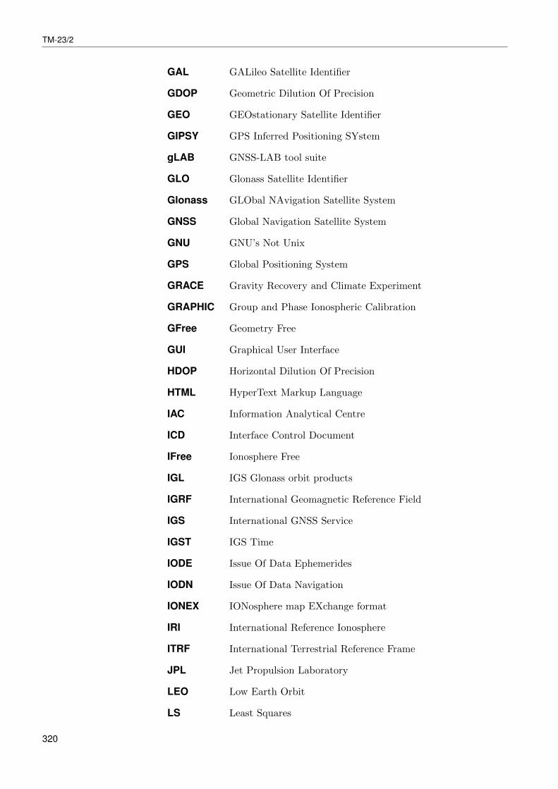
TM-23/2
GAL GALileo Satellite Identifier
GDOP Geometric Dilution Of Precision
GEO GEOstationary Satellite Identifier
GIPSY GPS Inferred Positioning SYstem
gLAB GNSS-LAB tool suite
GLO Glonass Satellite Identifier
Glonass GLObal NAvigation Satellite System
GNSS Global Navigation Satellite System
GNU GNU’s Not Unix
GPS Global Positioning System
GRACE Gravity Recovery and Climate Experiment
GRAPHIC Group and Phase Ionospheric Calibration
GFree Geometry Free
GUI Graphical User Interface
HDOP Horizontal Dilution Of Precision
HTML HyperText Markup Language
IAC Information Analytical Centre
ICD Interface Control Document
IFree Ionosphere Free
IGL IGS Glonass orbit products
IGRF International Geomagnetic Reference Field
IGS International GNSS Service
IGST IGS Time
IODE Issue Of Data Ephemerides
IODN Issue Of Data Navigation
IONEX IONosphere map EXchange format
IRI International Reference Ionosphere
ITRF International Terrestrial Reference Frame
JPL Jet Propulsion Laboratory
LEO Low Earth Orbit
LS Least Squares
320

List of Acronyms
LSTIDs Large-Scale TIDs
MC Satellite Mass Centre
MCC Mission Control Centre
MJD Modified Julian Day
MM Monument Marker
MSDOS Microsoft Disk Operating System
MSTID Medium-Scale Travelling Ionospheric Disturbance
MSTIDs Medium-Scale Travelling Ionospheric Disturbances
MW Melbourne–Wubbena
NANU Notice Advisory to NAVSTAR Users
NASA National Aeronautics and Space Administration
NEU North East Up
NGA National Geospatial-Intelligence Agency
NSE Navigation System Error
OS Operating System
PCO Phase Centre Offset
PCV Phase Centre Variation
PDOP Precision Dilution Of Precision
PNG Portable Network Graphics
PPP Precise Point Positioning
PRN Pseudo-Random Noise
PVT Position, Velocity, Time
PZ-90 Parametry Zemli 1990 (Parameters of Earth 1990)
RINEX Receiver INdependent EXchange format
RK4 Fourth-order Runge–Kutta
RMS Root Mean Square
RO Radio Occultation
S/A Selective Availability
SBAS Satellite-Based Augmentation System
SED Storm Enhancement Density
SINEX Solution (Software/technique) INdependent EXchange format
321
TM-23/2
SIS Signal In Space
SISRE Signal In Space Range Error
SOHO SOlar Helioscopic Observatory
SP3 Standard Product #3
SPP Standard Point Positioning
SPS Standard Positioning Service
SSI Signal Strength Indicator
STEC Slant Total Electron Content
STROP Slant TROPospheric delay
SU Soviet Union
SV Space Vehicle
SVN Space Vehicle Number
TDOP Time Dilution Of Precision
TEC Total Electron Content
TECU Total Electron Content Unit
TGD Total Group Delay
TID Travelling Ionospheric Disturbance
TRF Terrestrial Reference Frame
TRS Conventional Terrestrial Reference System
TUM Technische Universitat Munchen
UPC Technical University of Catalonia
USNO United States Naval Observatory
UTC Coordinated Universal Time
VDOP Vertical Dilution Of Precision
WGS-84 World Geodetic System 84
ZTD Zenith Tropospheric Delay
322