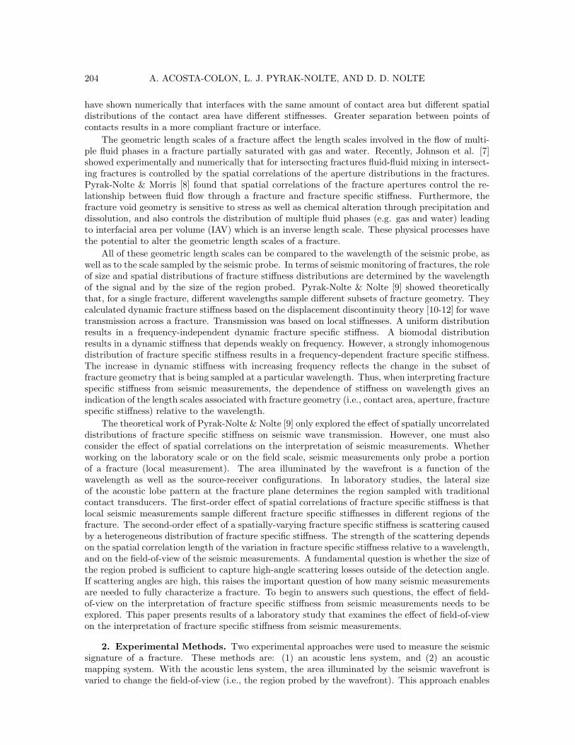
Proceedings of the Project Review, Geo-Mathematical Imaging Group (Purdue University, West Lafayette IN),Vol. 1 (2008) pp. 203-220.

LABORATORY-SCALE STUDY OF FIELD-OF-VIEW AND THE SEISMIC

INTERPRETATION OF FRACTURE SPECIFIC STIFFNESS

ANGEL ACOSTA-COLON∗, LAURA J. PYRAK-NOLTE† , AND DAVID D. NOLTE‡

Abstract. The effects of the scale of measurement, i.e., the field-of-view, on the interpretation of fractureproperties from seismic wave propagation was investigated using an acoustic lens system to produce pseudo-collimatedwavefronts. The incident wavefront had a controllable beam diameter that set the field-of-view at 15 mm, 30 mmand 60 mm. At a smaller scale, traditional acoustic scans were used to probe the fracture in 2 mm increments. Thislaboratory approach was applied to two limestone samples, each containing a single induced fracture, and comparedto an acrylic control sample. From the analysis of the average coherent sum of the signals measured on each scale, weobserved that the scale of the field-of-view affected the interpretation of fracture specific stiffness. Many small-scalemeasurements of the seismic response of a fracture, when summed, did not predict the large-scale response of thefracture. The change from a frequency-independent to a frequency-dependent fracture stiffness occurs when the scaleof the field-of-view exceeds the spatial correlation length associated with fracture geometry. A frequency-independentfracture specific stiffness is not sufficient to classify a fracture as homogeneous. A non-uniform spatial distributionof fracture specific stiffness and overlapping geometric scales in a fracture cause a scale-dependent seismic responsewhich requires measurements at different field-of-views to fully characterize the fracture.

1. Introduction. The scaling behavior of the hydraulic and seismic properties of a fracturedetermines how properties observed on the laboratory size (typically less than tens of cm) relate tothe same properties measured at larger sizes. In describing the scaling behavior of fracture prop-erties, the length scales of the fracture geometry (apertures, contact areas, spatial correlations),fluid phase distribution (wetting and non-wetting phase areas, interfacial areas), must be character-ized and compared to the length scales associated with the seismic probe (wavelength, beam size,divergence angle, field-of-view).

For fractures in rock, measurements on the laboratory scale encompass several different lengthscales that include the size of the sample and the size of the fracture. A single fracture can beviewed as two rough surfaces in contact that produce regions of contact and open voids in a quasi-two-dimensional fashion. This fracture geometry has many length scales that are described contactarea and its spatial distribution, as well as by the size (aperture) and spatial distribution of thevoid space. From laboratory measurements, Pyrak-Nolte et al. (1997) [1] found that the aperturedistribution of natural fracture networks in whole-drill coal cores were spatially correlated over 10mm to 30 mm, i.e., distances that were comparable to the size of the core samples. However,asperities on natural joint surfaces have been observed to be correlated over only about 0.5 mm [2]from surface roughness measurements. These two quoted values for correlation lengths vary by upto two orders of magnitude. The spatial correlation lengths are likely to be a function of rock type,but this needs to be verified experimentally. The observation that correlation lengths are smaller oron the same order as the sample size may explain why core samples often predict different hydraulic-mechanical behavior than is observed in the field. If a fracture on the core scale is correlated overa few centimeters, the same fracture on the field scale may behave as an uncorrelated fracture.

An additional length scale that is necessary to consider when investigating the scaling behavior ofseismic wave propagation across single fractures is the spatial variation in fracture specific stiffness.Fracture specific stiffness is defined as the ratio of the increment of stress to the increment ofdisplacement caused by the deformation of the void space in the fracture. As stress on the fractureincreases, the contact area between the two fracture surfaces also increases, raising the stiffness ofthe fracture. Fracture specific stiffness depends on the elastic properties of the rock and dependscritically on the amount and distribution of contact area in a fracture that arises from two roughsurfaces in contact [3-5]. Kendall & Tabor [6] showed experimentally and Hopkins et al. [4,5]

∗Department of Earth and Atmospheric Sciences, Purdue University, West Lafayette, Indiana 47907 (aa-costate@purdue.edu).

†Department of Physics, Purdue University, West Lafayette, Indiana 47907, Department of Earth and AtmosphericSciences, Purdue University, West Lafayette, Indiana 47907 (ljpn@physics.purdue.edu).

‡Department of Physics, Purdue University, West Lafayette, Indiana 47907 (nolte@physics.purdue.edu).

203

204 A. ACOSTA-COLON, L. J. PYRAK-NOLTE, AND D. D. NOLTE

have shown numerically that interfaces with the same amount of contact area but different spatialdistributions of the contact area have different stiffnesses. Greater separation between points ofcontacts results in a more compliant fracture or interface.

The geometric length scales of a fracture affect the length scales involved in the flow of multi-ple fluid phases in a fracture partially saturated with gas and water. Recently, Johnson et al. [7]showed experimentally and numerically that for intersecting fractures fluid-fluid mixing in intersect-ing fractures is controlled by the spatial correlations of the aperture distributions in the fractures.Pyrak-Nolte & Morris [8] found that spatial correlations of the fracture apertures control the re-lationship between fluid flow through a fracture and fracture specific stiffness. Furthermore, thefracture void geometry is sensitive to stress as well as chemical alteration through precipitation anddissolution, and also controls the distribution of multiple fluid phases (e.g. gas and water) leadingto interfacial area per volume (IAV) which is an inverse length scale. These physical processes havethe potential to alter the geometric length scales of a fracture.

All of these geometric length scales can be compared to the wavelength of the seismic probe, aswell as to the scale sampled by the seismic probe. In terms of seismic monitoring of fractures, the roleof size and spatial distributions of fracture stiffness distributions are determined by the wavelengthof the signal and by the size of the region probed. Pyrak-Nolte & Nolte [9] showed theoreticallythat, for a single fracture, different wavelengths sample different subsets of fracture geometry. Theycalculated dynamic fracture stiffness based on the displacement discontinuity theory [10-12] for wavetransmission across a fracture. Transmission was based on local stiffnesses. A uniform distributionresults in a frequency-independent dynamic fracture specific stiffness. A biomodal distributionresults in a dynamic stiffness that depends weakly on frequency. However, a strongly inhomogenousdistribution of fracture specific stiffness results in a frequency-dependent fracture specific stiffness.The increase in dynamic stiffness with increasing frequency reflects the change in the subset offracture geometry that is being sampled at a particular wavelength. Thus, when interpreting fracturespecific stiffness from seismic measurements, the dependence of stiffness on wavelength gives anindication of the length scales associated with fracture geometry (i.e., contact area, aperture, fracturespecific stiffness) relative to the wavelength.

The theoretical work of Pyrak-Nolte & Nolte [9] only explored the effect of spatially uncorrelateddistributions of fracture specific stiffness on seismic wave transmission. However, one must alsoconsider the effect of spatial correlations on the interpretation of seismic measurements. Whetherworking on the laboratory scale or on the field scale, seismic measurements only probe a portionof a fracture (local measurement). The area illuminated by the wavefront is a function of thewavelength as well as the source-receiver configurations. In laboratory studies, the lateral sizeof the acoustic lobe pattern at the fracture plane determines the region sampled with traditionalcontact transducers. The first-order effect of spatial correlations of fracture specific stiffness is thatlocal seismic measurements sample different fracture specific stiffnesses in different regions of thefracture. The second-order effect of a spatially-varying fracture specific stiffness is scattering causedby a heterogeneous distribution of fracture specific stiffness. The strength of the scattering dependson the spatial correlation length of the variation in fracture specific stiffness relative to a wavelength,and on the field-of-view of the seismic measurements. A fundamental question is whether the size ofthe region probed is sufficient to capture high-angle scattering losses outside of the detection angle.If scattering angles are high, this raises the important question of how many seismic measurementsare needed to fully characterize a fracture. To begin to answers such questions, the effect of field-of-view on the interpretation of fracture specific stiffness from seismic measurements needs to beexplored. This paper presents results of a laboratory study that examines the effect of field-of-viewon the interpretation of fracture specific stiffness from seismic measurements.

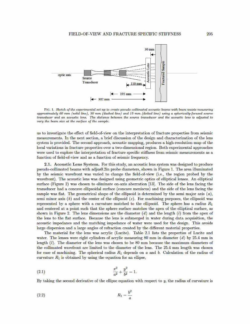
2. Experimental Methods. Two experimental approaches were used to measure the seismicsignature of a fracture. These methods are: (1) an acoustic lens system, and (2) an acousticmapping system. With the acoustic lens system, the area illuminated by the seismic wavefront isvaried to change the field-of-view (i.e., the region probed by the wavefront). This approach enables

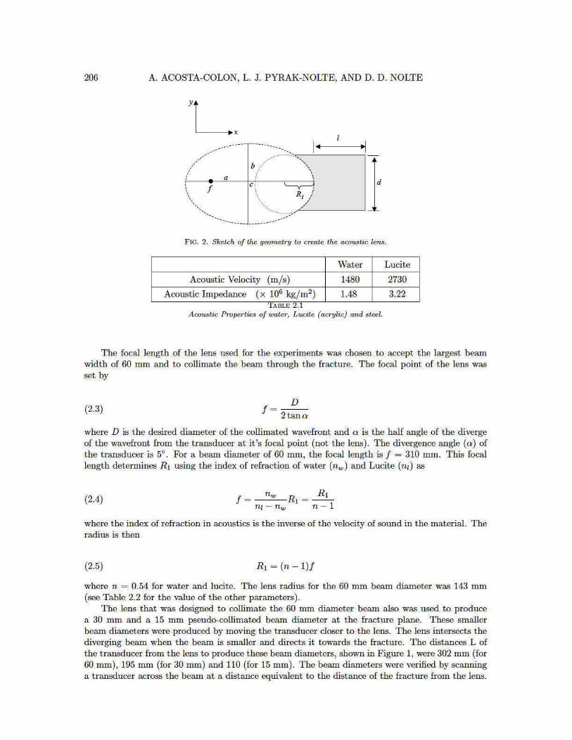
FIELD-OF-VIEW AND FRACTURE SPECIFIC STIFFNESS 207

Design Value

R1 143.02mm

a 202.52mm

b 170.19mm

l 25.4mm

d 80mm

material LuciteTable 2.2

Values for the design of the acoustic lens.

(a) 110 mm (b) 195 mm

(c) 302 mm

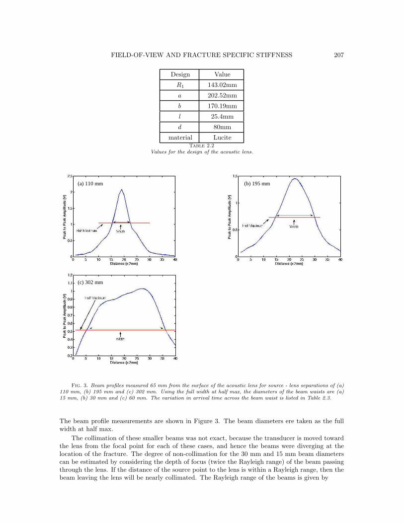
Fig. 3. Beam profiles measured 65 mm from the surface of the acoustic lens for source - lens separations of (a)110 mm, (b) 195 mm and (c) 302 mm. Using the full width at half max, the diameters of the beam waists are (a)15 mm, (b) 30 mm and (c) 60 mm. The variation in arrival time across the beam waist is listed in Table 2.3.

The beam profile measurements are shown in Figure 3. The beam diameters ere taken as the fullwidth at half max.

The collimation of these smaller beams was not exact, because the transducer is moved towardthe lens from the focal point for each of these cases, and hence the beams were diverging at thelocation of the fracture. The degree of non-collimation for the 30 mm and 15 mm beam diameterscan be estimated by considering the depth of focus (twice the Rayleigh range) of the beam passingthrough the lens. If the distance of the source point to the lens is within a Rayleigh range, then thebeam leaving the lens will be nearly collimated. The Rayleigh range of the beams is given by

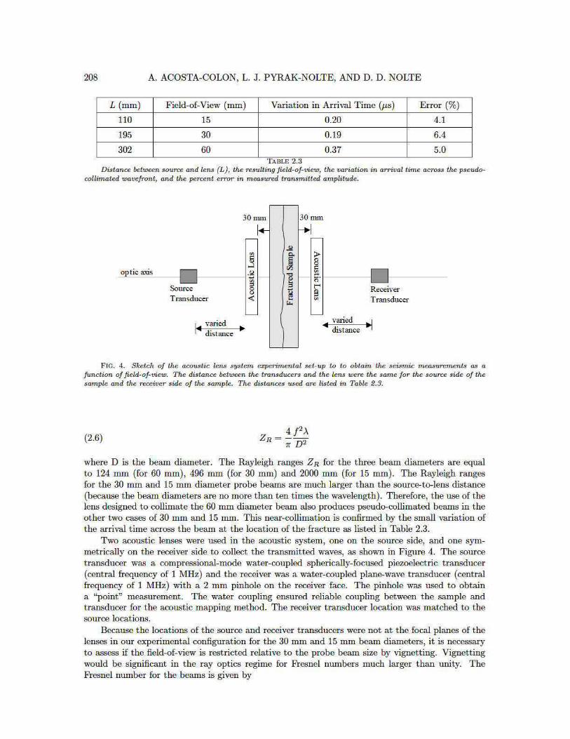
FIELD-OF-VIEW AND FRACTURE SPECIFIC STIFFNESS 209

(2.7) NF =D2

Lλ

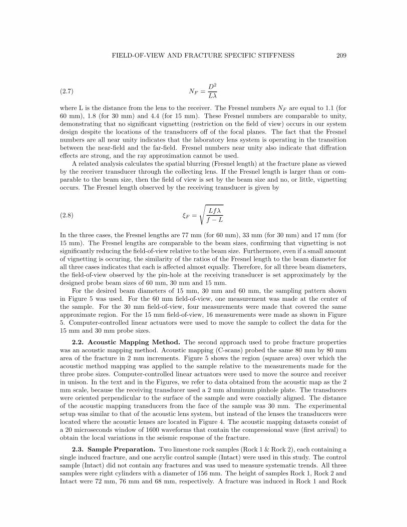
where L is the distance from the lens to the receiver. The Fresnel numbers NF are equal to 1.1 (for60 mm), 1.8 (for 30 mm) and 4.4 (for 15 mm). These Fresnel numbers are comparable to unity,demonstrating that no significant vignetting (restriction on the field of view) occurs in our systemdesign despite the locations of the transducers off of the focal planes. The fact that the Fresnelnumbers are all near unity indicates that the laboratory lens system is operating in the transitionbetween the near-field and the far-field. Fresnel numbers near unity also indicate that diffrationeffects are strong, and the ray approximation cannot be used.

A related analysis calculates the spatial blurring (Fresnel length) at the fracture plane as viewedby the receiver transducer through the collecting lens. If the Fresnel length is larger than or com-parable to the beam size, then the field of view is set by the beam size and no, or little, vignettingoccurs. The Fresnel length observed by the receiving transducer is given by

(2.8) ξF =

√

Lfλ

f − L

In the three cases, the Fresnel lengths are 77 mm (for 60 mm), 33 mm (for 30 mm) and 17 mm (for15 mm). The Fresnel lengths are comparable to the beam sizes, confirming that vignetting is notsignificantly reducing the field-of-view relative to the beam size. Furthermore, even if a small amountof vignetting is occuring, the similarity of the ratios of the Fresnel length to the beam diameter forall three cases indicates that each is affected almost equally. Therefore, for all three beam diameters,the field-of-view observed by the pin-hole at the receiving transducer is set approximately by thedesigned probe beam sizes of 60 mm, 30 mm and 15 mm.

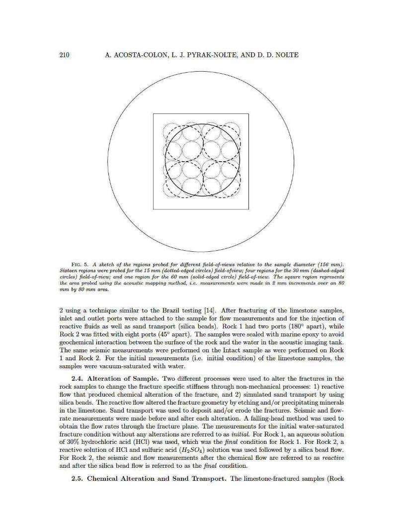
For the desired beam diameters of 15 mm, 30 mm and 60 mm, the sampling pattern shownin Figure 5 was used. For the 60 mm field-of-view, one measurement was made at the center ofthe sample. For the 30 mm field-of-view, four measurements were made that covered the sameapproximate region. For the 15 mm field-of-view, 16 measurements were made as shown in Figure5. Computer-controlled linear actuators were used to move the sample to collect the data for the15 mm and 30 mm probe sizes.

2.2. Acoustic Mapping Method. The second approach used to probe fracture propertieswas an acoustic mapping method. Acoustic mapping (C-scans) probed the same 80 mm by 80 mmarea of the fracture in 2 mm increments. Figure 5 shows the region (square area) over which theacoustic method mapping was applied to the sample relative to the measurements made for thethree probe sizes. Computer-controlled linear actuators were used to move the source and receiverin unison. In the text and in the Figures, we refer to data obtained from the acoustic map as the 2mm scale, because the receiving transducer used a 2 mm aluminum pinhole plate. The transducerswere oriented perpendicular to the surface of the sample and were coaxially aligned. The distanceof the acoustic mapping transducers from the face of the sample was 30 mm. The experimentalsetup was similar to that of the acoustic lens system, but instead of the lenses the transducers werelocated where the acoustic lenses are located in Figure 4. The acoustic mapping datasets consist ofa 20 microseconds window of 1600 waveforms that contain the compressional wave (first arrival) toobtain the local variations in the seismic response of the fracture.

2.3. Sample Preparation. Two limestone rock samples (Rock 1 & Rock 2), each containing asingle induced fracture, and one acrylic control sample (Intact) were used in this study. The controlsample (Intact) did not contain any fractures and was used to measure systematic trends. All threesamples were right cylinders with a diameter of 156 mm. The height of samples Rock 1, Rock 2 andIntact were 72 mm, 76 mm and 68 mm, respectively. A fracture was induced in Rock 1 and Rock

FIELD-OF-VIEW AND FRACTURE SPECIFIC STIFFNESS 211

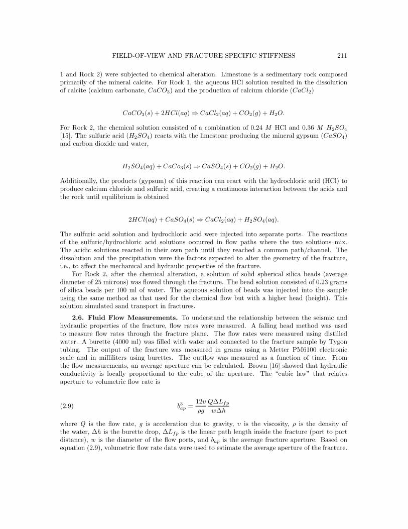
1 and Rock 2) were subjected to chemical alteration. Limestone is a sedimentary rock composedprimarily of the mineral calcite. For Rock 1, the aqueous HCl solution resulted in the dissolutionof calcite (calcium carbonate, CaCO3) and the production of calcium chloride (CaCl2)

CaCO3(s) + 2HCl(aq) ⇒ CaCl2(aq) + CO2(g) + H2O.

For Rock 2, the chemical solution consisted of a combination of 0.24 M HCl and 0.36 M H2SO4

[15]. The sulfuric acid (H2SO4) reacts with the limestone producing the mineral gypsum (CaSO4)and carbon dioxide and water,

H2SO4(aq) + CaCo3(s) ⇒ CaSO4(s) + CO2(g) + H2O.

Additionally, the products (gypsum) of this reaction can react with the hydrochloric acid (HCl) toproduce calcium chloride and sulfuric acid, creating a continuous interaction between the acids andthe rock until equilibrium is obtained

2HCl(aq) + CaSO4(s) ⇒ CaCl2(aq) + H2SO4(aq).

The sulfuric acid solution and hydrochloric acid were injected into separate ports. The reactionsof the sulfuric/hydrochloric acid solutions occurred in flow paths where the two solutions mix.The acidic solutions reacted in their own path until they reached a common path/channel. Thedissolution and the precipitation were the factors expected to alter the geometry of the fracture,i.e., to affect the mechanical and hydraulic properties of the fracture.

For Rock 2, after the chemical alteration, a solution of solid spherical silica beads (averagediameter of 25 microns) was flowed through the fracture. The bead solution consisted of 0.23 gramsof silica beads per 100 ml of water. The aqueous solution of beads was injected into the sampleusing the same method as that used for the chemical flow but with a higher head (height). Thissolution simulated sand transport in fractures.

2.6. Fluid Flow Measurements. To understand the relationship between the seismic andhydraulic properties of the fracture, flow rates were measured. A falling head method was usedto measure flow rates through the fracture plane. The flow rates were measured using distilledwater. A burette (4000 ml) was filled with water and connected to the fracture sample by Tygontubing. The output of the fracture was measured in grams using a Metter PM6100 electronicscale and in milliliters using burettes. The outflow was measured as a function of time. Fromthe flow measurements, an average aperture can be calculated. Brown [16] showed that hydraulicconductivity is locally proportional to the cube of the aperture. The “cubic law” that relatesaperture to volumetric flow rate is

(2.9) b3ap =

12υ

ρg

Q∆Lfp

w∆h

where Q is the flow rate, g is acceleration due to gravity, υ is the viscosity, ρ is the density ofthe water, ∆h is the burette drop, ∆Lfp is the linear path length inside the fracture (port to portdistance), w is the diameter of the flow ports, and bap is the average fracture aperture. Based onequation (2.9), volumetric flow rate data were used to estimate the average aperture of the fracture.

212 A. ACOSTA-COLON, L. J. PYRAK-NOLTE, AND D. D. NOLTE

3. DATA ANALYSIS.

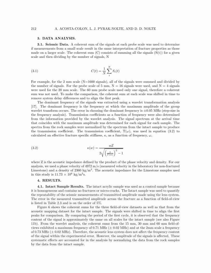
3.1. Seismic Data. A coherent sum of the signals at each probe scale was used to determineif measurements from a small scale result in the same interpretation of fracture properties as thosemade on a larger scale. The coherent sum (C) consists of summing all the signals (S(t)) for a givenscale and then dividing by the number of signals, N

(3.1) C(t) =1

N

N∑

i

Si(t)

For example, for the 2 mm scale (N=1600 signals), all of the signals were summed and divided bythe number of signals. For the probe scale of 5 mm, N = 16 signals were used, and N = 4 signalswere used for the 20 mm scale. The 60 mm probe scale used only one signal, therefore a coherentsum was not used. To make the comparison, the coherent sum at each scale was shifted in time toremove system delay differences and to align the first peak.

The dominant frequency of the signals was extracted using a wavelet transformation analysis[17]. The dominant frequency is the frequency at which the maximum amplitude of the groupwavelet transform occurs. The error in choosing the dominant frequency is ±0.05 MHz (step-size inthe frequency analysis). Transmission coefficients as a function of frequency were also determinedfrom the information provided by the wavelet analysis. The signal spectrum at the arrival timethat coincides with the maximum amplitude was determined for each signal for each sample. Thespectra from the rock samples were normalized by the spectrum from the intact sample to producethe transmission coefficient. The transmission coefficient, T(ω), was used in equation (3.2) tocalculated an effective fracture specific stiffness, κ, as a function of frequency, ω,

(3.2) κ(w) =wZ

2

√

(

1T (w)

)2

− 1

where Z is the acoustic impedance defined by the product of the phase velocity and density. For ouranalysis, we used a phase velocity of 4972 m/s (measured velocity in the laboratory for non-fracturedLimestone) and a density of 2360 kg/m3. The acoustic impedance for the Limestone samples usedin this study is 11.73 × 106 kg/m2s.

4. RESULTS.

4.1. Intact Sample Results. The intact acrylic sample was used as a control sample becauseit is homogeneous and contains no fractures or micro-cracks. The Intact sample was used to quantifythe repeatability of the seismic measurements of transmitted amplitude made using the lens system.The error in the measured transmitted amplitude across the fracture as a function of field-of-viewis listed in Table 2.3 and is on the order of 5%.

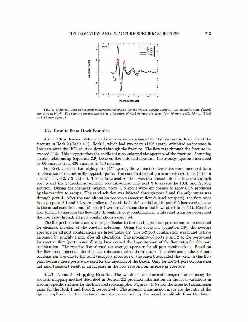
Figure 6 shows the coherent sums for the three field-of-view datasets as well as that from theacoustic mapping dataset for the intact sample. The signals were shifted in time to align the firstpeaks for comparison. By comparing the period of the first cycle, it is observed that the frequencycontent of the signal is approximately the same on all scales for the intact sample (see also Figure11b). From the wavelet analysis, the coherent sums from the 15 mm, 30 mm and 60 mm field-of-views exhibited a maximum frequency of 0.71 MHz (± 0.02 MHz) and at the 2mm scale a frequencyof 0.73 MHz (± 0.02 MHz). Therefore, the acoustic lens system does not affect the frequency contentof the signal within the experimental error. However, the amplitude of the signals is affected. Thesesystematic effects are accounted for in the analysis by normalizing the data from the rock samplesby the data from the intact sample.

214 A. ACOSTA-COLON, L. J. PYRAK-NOLTE, AND D. D. NOLTE

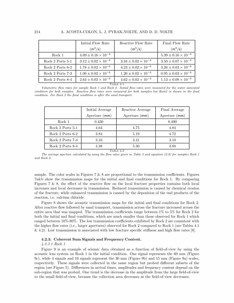
Initial Flow Rate Reactive Flow Rate Final Flow Rate

(m3/s) (m3/s) (m3/s)

Rock 1 4.09 ± 0.16 × 10−8 5.39 ± 0.16 × 10−8

Rock 2 Ports 5-1 3.12 ± 0.02 × 10−6 3.34 ± 0.02 × 10−6 3.50 ± 0.07 × 10−6

Rock 2 Ports 6-2 1.78 ± 0.02 × 10−6 4.23 ± 0.02 × 10−6 3.26 ± 0.03 × 10−6

Rock 2 Ports 7-3 1.00 ± 0.02 × 10−6 1.26 ± 0.02 × 10−6 0.95 ± 0.03 × 10−6

Rock 2 Ports 8-4 2.64 ± 0.02 × 10−6 4.62 ± 0.02 × 10−6 1.13 ± 0.08 × 10−6

Table 4.1

Volumetric flow rates for sample Rock 1 and Rock 2. Initial flow rates were measured for the water saturatedcondition for both samples. Reactive flow rates were measured for both samples but Rock1 is shown in the finalcondition. For Rock 2 the final condition is after the sand transport.

Initial Average Reactive Average Final Average

Aperture (mm) Aperture (mm) Aperture (mm)

Rock 1 0.430 0.490

Rock 2 Ports 5-1 4.64 4.75 4.84

Rock 2 Ports 6-2 3.84 5.19 4.72

Rock 2 Ports 7-3 3.16 3.41 3.10

Rock 2 Ports 8-4 4.38 5.30 3.88Table 4.2

The average aperture calculated by using the flow rates given in Table 3 and equation (2.9) for samples Rock 1and Rock 2.

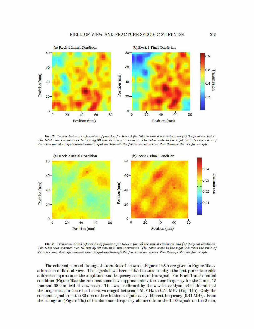
sample. The color scales in Figures 7 & 8 are proportional to the transmission coefficients. Figures7a&b show the transmission maps for the initial and final conditions for Rock 1. By comparingFigures 7 & 8, the effect of the reactive flow on the local fracture properties contains both localincreases and local decreases in transmission. Reduced transmission is caused by chemical erosionof the fracture, while enhanced transmission is caused by the deposition of the end products of thereaction, i.e. calcium chloride.

Figure 8 shows the acoustic transmission maps for the initial and final conditions for Rock 2.After reactive flow followed by sand transport, transmission across the fracture increased across theentire area that was mapped. The transmission coefficients range between 1% to 5% for Rock 2 forboth the initial and final conditions, which are much smaller than those observed for Rock 1 whichranged between 10%-80%. The low transmission coefficients exhibited by Rock 2 are consistent withthe higher flow rates (i.e., larger apertures) observed for Rock 2 compared to Rock 1 (see Tables 4.1& 4.2). Low transmission is associated with low fracture specific stiffness and high flow rates [8].

4.2.3. Coherent Sum Signals and Frequency Content.

4.2.3.1 Rock 1

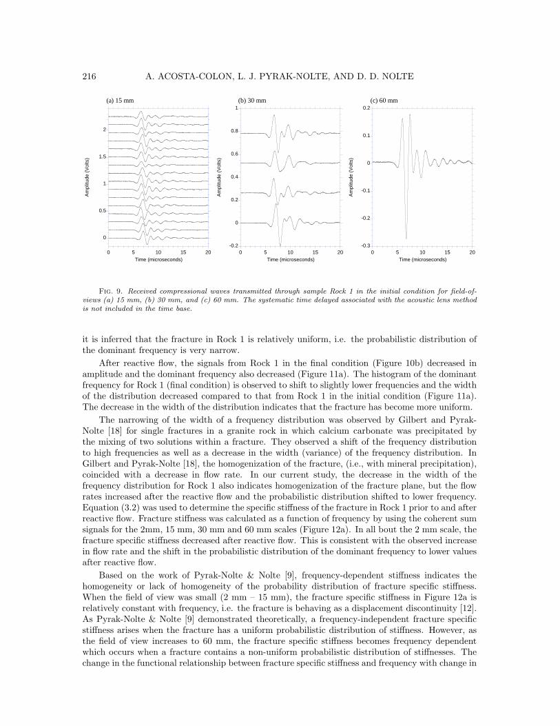
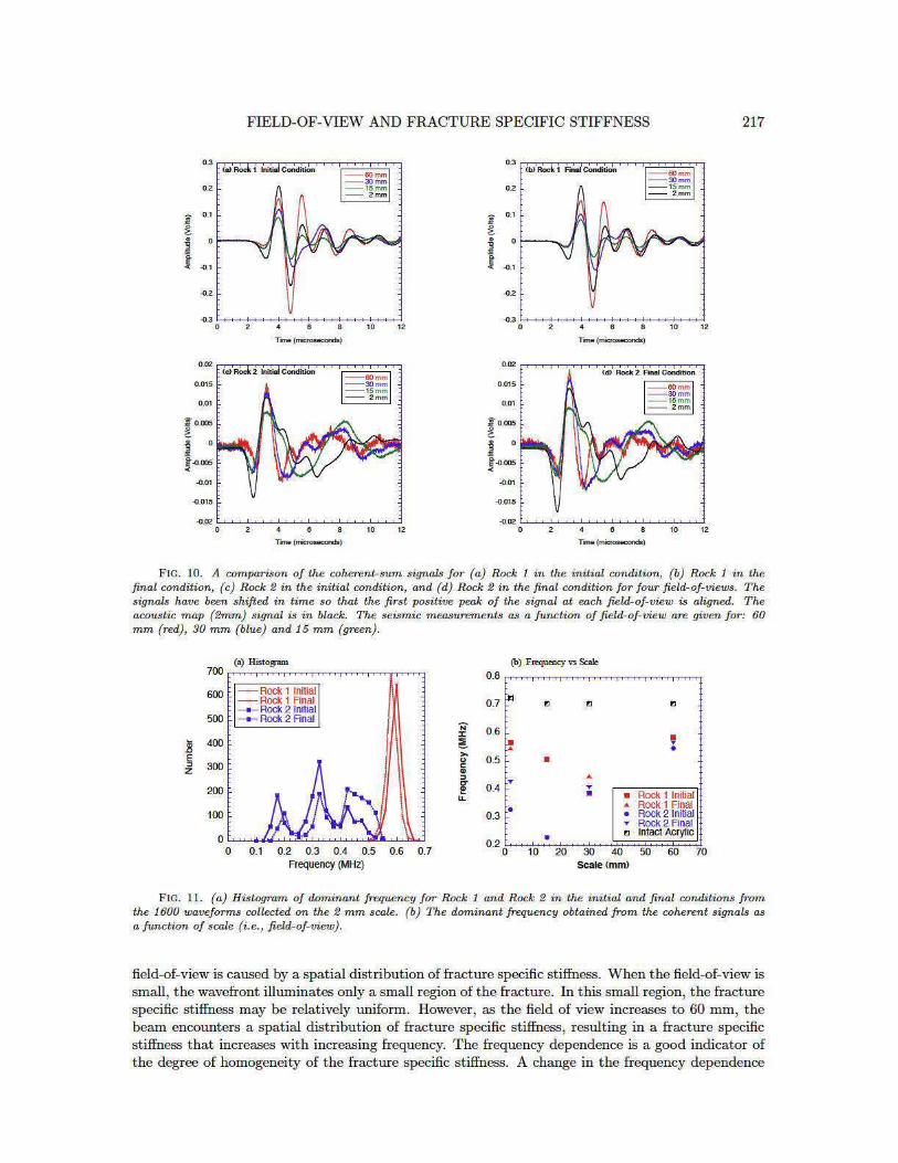
Figure 9 is an example of seismic data obtained as a function of field-of-view by using theacoustic lens system on Rock 1 in the initial condition. One signal represents the 60 mm (Figure9c), while 4 signals and 16 signals represent the 30 mm (Figure 9b) and 15 mm (Figure 9a) scales,respectively. These signals were collected in the same region but probed different subsets of theregion (see Figure 5). Differences in arrival times, amplitudes and frequency content depend on thesub-region that was probed. One trend is the decrease in the amplitude from the large field-of-viewto the small field-of-view, because the collection area decreases as the field-of-view decreases.

216 A. ACOSTA-COLON, L. J. PYRAK-NOLTE, AND D. D. NOLTE

0

0.5

1

1.5

2

0 5 10 15 20

Am

plitu

de (

Vol

ts)

Time (microseconds)

-0.2

0

0.2

0.4

0.6

0.8

1

0 5 10 15 20

Am

plitu

de (

Vol

ts)

Time (microseconds)

-0.3

-0.2

-0.1

0

0.1

0.2

0 5 10 15 20

Am

plitu

de (

Vol

ts)

Time (microseconds)

(a) 15 mm (b) 30 mm (c) 60 mm

Fig. 9. Received compressional waves transmitted through sample Rock 1 in the initial condition for field-of-views (a) 15 mm, (b) 30 mm, and (c) 60 mm. The systematic time delayed associated with the acoustic lens methodis not included in the time base.

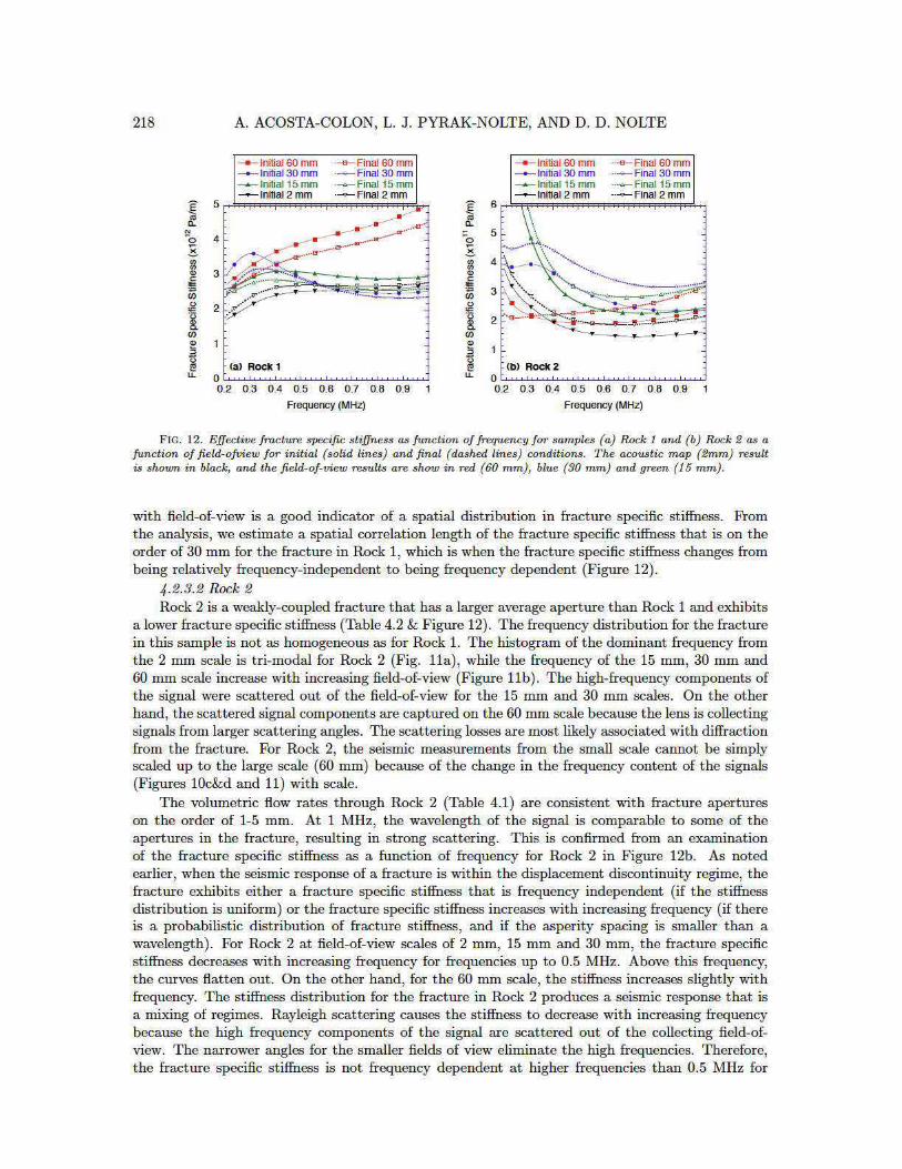
it is inferred that the fracture in Rock 1 is relatively uniform, i.e. the probabilistic distribution ofthe dominant frequency is very narrow.

After reactive flow, the signals from Rock 1 in the final condition (Figure 10b) decreased inamplitude and the dominant frequency also decreased (Figure 11a). The histogram of the dominantfrequency for Rock 1 (final condition) is observed to shift to slightly lower frequencies and the widthof the distribution decreased compared to that from Rock 1 in the initial condition (Figure 11a).The decrease in the width of the distribution indicates that the fracture has become more uniform.

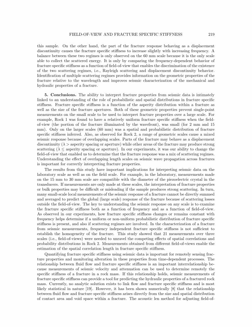
The narrowing of the width of a frequency distribution was observed by Gilbert and Pyrak-Nolte [18] for single fractures in a granite rock in which calcium carbonate was precipitated bythe mixing of two solutions within a fracture. They observed a shift of the frequency distributionto high frequencies as well as a decrease in the width (variance) of the frequency distribution. InGilbert and Pyrak-Nolte [18], the homogenization of the fracture, (i.e., with mineral precipitation),coincided with a decrease in flow rate. In our current study, the decrease in the width of thefrequency distribution for Rock 1 also indicates homogenization of the fracture plane, but the flowrates increased after the reactive flow and the probabilistic distribution shifted to lower frequency.Equation (3.2) was used to determine the specific stiffness of the fracture in Rock 1 prior to and afterreactive flow. Fracture stiffness was calculated as a function of frequency by using the coherent sumsignals for the 2mm, 15 mm, 30 mm and 60 mm scales (Figure 12a). In all bout the 2 mm scale, thefracture specific stiffness decreased after reactive flow. This is consistent with the observed increasein flow rate and the shift in the probabilistic distribution of the dominant frequency to lower valuesafter reactive flow.

Based on the work of Pyrak-Nolte & Nolte [9], frequency-dependent stiffness indicates thehomogeneity or lack of homogeneity of the probability distribution of fracture specific stiffness.When the field of view was small (2 mm – 15 mm), the fracture specific stiffness in Figure 12a isrelatively constant with frequency, i.e. the fracture is behaving as a displacement discontinuity [12].As Pyrak-Nolte & Nolte [9] demonstrated theoretically, a frequency-independent fracture specificstiffness arises when the fracture has a uniform probabilistic distribution of stiffness. However, asthe field of view increases to 60 mm, the fracture specific stiffness becomes frequency dependentwhich occurs when a fracture contains a non-uniform probabilistic distribution of stiffnesses. Thechange in the functional relationship between fracture specific stiffness and frequency with change in

FIELD-OF-VIEW AND FRACTURE SPECIFIC STIFFNESS 219

this sample. On the other hand, the part of the fracture response behaving as a displacementdiscontinuity causes the fracture specific stiffness to increase slightly with increasing frequency. Abalance between these two regimes is only observed on the 60 mm scale because it is the only scaleable to collect the scattered energy. It is only by comparing the frequency-dependent behavior offracture specific stiffness as a function of field-of-view that enables the discrimination of the existenceof the two scattering regimes, i.e., Rayleigh scattering and displacement discontinuity behavior.Identification of multiple scattering regimes provides information on the geometric properties of thefracture relative to the wavelength and improves seismic characterization of the mechanical andhydraulic properties of a fracture.

5. Conclusions. The ability to interpret fracture properties from seismic data is intimatelylinked to an understanding of the role of probabilistic and spatial distributions in fracture specificstiffness. Fracture specific stiffness is a function of the asperity distribution within a fracture aswell as the size of the fracture apertures. Both of these geometric properties prevent single-pointmeasurements on the small scale to be used to interpret fracture properties over a large scale. Forexample, Rock 1 was found to have a relatively uniform fracture specific stiffness when the field-of-view (the portion of the fracture illuminated by the wavefront), was small (for 2 mm and 15mm). Only on the larger scales (60 mm) was a spatial and probabilistic distribution of fracturespecific stiffness inferred. Also, as observed for Rock 2, a range of geometric scales cause a mixedseismic response because of overlapping scales. Parts of the fracture may behave as a displacementdiscontinuity (λ > asperity spacing or aperture) while other areas of the fracture may produce strongscattering (λ ≤ asperity spacing or aperture). In our experiments, it was our ability to change thefield-of-view that enabled us to determine that the fracture response was a mix of scattering regimes.Understanding the effect of overlapping length scales on seismic wave propagation across fracturesis important for correctly interpreting fracture properties.

The results from this study have important implications for interpreting seismic data on thelaboratory scale as well as on the field scale. For example, in the laboratory, measurements madeon the 15 mm to 30 mm scale are compatible with the diameter of the piezoelectric crystal in thetransducers. If measurements are only made at these scales, the interpretation of fracture propertiesor bulk properties may be difficult or misleading if the sample produces strong scattering. In turn,many small-scale local measurements of the seismic response of a fracture cannot be directly summedand averaged to predict the global (large scale) response of the fracture because of scattering lossesoutside the field-of-view. The key to understanding the seismic response on any scale is to examinethe fracture specific stiffness both as a function of frequency and as a function of field-of-view.As observed in our experiments, how fracture specific stiffness changes or remains constant withfrequency helps determine if a uniform or non-uniform probabilistic distribution of fracture specificstiffness is present, and also if scattering regimes are involved. In the characterization of a fracturefrom seismic measurements, frequency independent fracture specific stiffness is not sufficient toestablish the homogeneity of the fracture. This study showed that 21 measurements over threescales (i.e., field-of-views) were needed to unravel the competing effects of spatial correlations andprobability distributions in Rock 2. Measurements obtained from different field-of-views enable theestimation of the spatial correlation length in fracture specific stiffness.

Quantifying fracture specific stiffness using seismic data is important for remotely sensing frac-ture properties and monitoring alteration in these properties from time-dependent processes. Therelationship between fluid flow and fracture specific stiffness is an important interrelationship be-cause measurements of seismic velocity and attenuation can be used to determine remotely thespecific stiffness of a fracture in a rock mass. If this relationship holds, seismic measurements offracture specific stiffness can provide a tool for predicting the hydraulic properties of a fractured rockmass. Currently, no analytic solution exists to link flow and fracture specific stiffness and is mostlikely statistical in nature [19]. However, it has been shown numerically [8] that the relationshipbetween fluid flow and fracture specific stiffness arises directly from the size and spatial distributionof contact area and void space within a fracture. The acoustic len method for adjusting field-of-

220 A. ACOSTA-COLON, L. J. PYRAK-NOLTE, AND D. D. NOLTE

view demonstrated that information on spatial distributions in fracture properties is achievable fromseismic measurements.

Acknowledgments. The authors wish to acknowledge support of this work by the GeosciencesResearch Program, Office of Basic Energy Sciences US Department of Energy (DEFG02-97ER1478508). Also AAC acknowledges the Rock Physics Group at Purdue University for the help during thiswork.

REFERENCES

[1] Pyrak-Nolte, L.J., C.D. Montemagno, and D.D. Nolte, Volumetric imaging of aperture distributions inconnected fracture networks. Geophysical Research Letters, 1997. 24(18): p. 2343-2346.

[2] Brown, S.R., R.L. Kranz, and B.P. Bonner, Correlation between surfaces of natural rock joints. GeophysicalResearch Letters, 1986. 13: p. 1430-1434.

[3] Brown, S.R. and C.H. Scholz, Closure of random surfaces in contact. Journal of Geophysical Research, 1985.90: p. 5531.

[4] Hopkins, D.L., The Effect of Surface Roughness on Joint Stiffness, Aperture and Acoustic Wave Propagation.1990, University of California, Berkeley: Berkeley.

[5] Hopkins, D.L., N.G.W. Cook, and L.R. Myer. Fracture stiffness and aperture as a function of applied stressand contact geometry. in 28th US Symposium on Rock Mechanics. 1987. Tucson, Arizona: A. A. Balkema.

[6] Kendall, K. and D. Tabor, An ultrasonic study of the area of contact between stationary and sliding surfaces.Proc. Royal Soc. London, Series A., 1971. 323: p. 321-340.

[7] Johnson, J., S.R. Brown, and H.W. Stockman, Fluid flow and mixing in rough-walled fracture intersections.Journal of Geophysical Research, 2006. 111(B12206): p. doi:10.1029/2005JB004087.

[8] Pyrak-Nolte, L.J. and J.P. Morris, Single fractures under normal stress: The relation between fracturespecific stiffness and fluid flow. International Journal of Rock Mechanics and Mining Sciences, 2000. 37(1-2): p. 245-262.

[9] Pyrak-Nolte, L.J. and D.D. Nolte, Frequency-Dependence of Fracture Stiffness. Geophysical Research Let-ters, 1992. 19(3): p. 325-328.

[10] Schoenberg, M., Elastic wave behavior across linear slip interfaces. Journal of the Acoustical Society ofAmerica, 1980. 5(68): p. 1516-1521.

[11] Gu, B.L., K.T. Nihei, L.R. Myer, and L.J. Pyrak-Nolte, Fracture interface waves. Journal of GeophysicalResearch-Solid Earth, 1996. 101(B1): p. 827-835.

[12] Pyrak-Nolte, L.J., L.R. Myer, and N.G.W. Cook, Transmission of Seismic-Waves across Single NaturalFractures. Journal of Geophysical Research-Solid Earth and Planets, 1990. 95(B6): p. 8617-8638.

[13] Dunn, F. and F.J. Fry, Acoustic elliptic lenses - an historical note. Journal of the Acoustical Society ofAmerica, 1980. 68(1): p. 350-351.

[14] Jaeger, J.C. and N.G.W. Cook, Fundamentals of Rock Mechancis. 1972, London: Methuen & Co, KTD.[15] Singurindy, O. and B. Berkowitz, Evolution of the hydraulic conductivity by precipitation and dissolution

in carbonate rock. Water Resources Research, 2003. 39(1): p. 1016.[16] Brown, S.R., Fluid flow through rock joints: The effect of surface roughness. Journal of Geophysical Research,

1987. 92: p. 1337-1347.[17] Nolte, D.D., Pyrak-Nolte, L. J., Beachy, J., and C. Ziegler, Transition from the displacement discon-

tinuity limit to the resonant scattering regime for fracture interface waves. International Journal of RockMechanics and Mining Sciences, 2000. 37(1-2): p. 219-230.

[18] Gilbert, Z., and L. J. Pyrak-Nolte, Seismic monitoring of fracture alteration by mineral deposition. in 6thNorth American Rock Mechanics Symposium. 2004. Houston, Texas.

[19] Jaeger, J.C., N.G.W. Cook, and R. Zimmerman, Fundamentals of Rock Mechanics, 4th Edition. 2007:Wiley-Blackwell.