Labs For Collaborative Statistics - Teegarden2.2.pdf... · Chapter 1 Candy Lab 1 Candy Lab Name: 1.1 Student Learning Outcomes The student will construct Relative requencyF ables.T

Labs For Collaborative Statistics -Teegarden

By:Mary Teegarden

Labs For Collaborative Statistics -Teegarden

By:Mary Teegarden

Online:< http://cnx.org/content/col10562/1.2/ >

C O N N E X I O N S

Rice University, Houston, Texas

This selection and arrangement of content as a collection is copyrighted by Mary Teegarden. It is licensed under the

Creative Commons Attribution 2.0 license (http://creativecommons.org/licenses/by/2.0/).

Collection structure revised: August 18, 2008

PDF generated: October 26, 2012

For copyright and attribution information for the modules contained in this collection, see p. 54.

Table of Contents

1 Candy Lab . . . . . . . . . . . . . . . . . . . . . . . . . . . . . . . . . . . . . . . . . . . . . . . . . . . . . . . . . . . . . . . . . . . . . . . . . . . . . . . . . . . . . . . . . 12 Descriptive Statistics: Descriptive Statistics Lab (edited: Teegarden) . . . . . . . . . . . . . . . . . . . . . . . 53 Probability Topics: Probability Lab (edited: Teegarden) . . . . . . . . . . . . . . . . . . . . . . . . . . . . . . . . . . . . . 74 Discrete Random Variables: Lab I (edited: Teegarden) . . . . . . . . . . . . . . . . . . . . . . . . . . . . . . . . . . . . . . 115 Continuous Random Variables: Lab I . . . . . . . . . . . . . . . . . . . . . . . . . . . . . . . . . . . . . . . . . . . . . . . . . . . . . . . . . . 156 Normal Distribution: Normal Distribution Lab I (edited: Teegarden) . . . . . . . . . . . . . . . . . . . . . 177 Central Limit Theorem: Central Limit Theorem Lab I (edited: Teegar-

den) . . . . . . . . . . . . . . . . . . . . . . . . . . . . . . . . . . . . . . . . . . . . . . . . . . . . . . . . . . . . . . . . . . . . . . . . . . . . . . . . . . . . . . . . . . . . 198 Con�dence Intervals: Con�dence Interval Lab I (edited: Teegarden) . . . . . . . . . . . . . . . . . . . . . . 259 Con�dence Intervals: Con�dence Interval Lab II (edited: Teegarden) . . . . . . . . . . . . . . . . . . . . . 2910 Con�dence Intervals: Con�dence Interval Lab III (edited: Teegarden) . . . . . . . . . . . . . . . . . . . 3111 Hypothesis Testing of Single Mean and Single Proportion: Lab (Edited:

Teegarden) 02 . . . . . . . . . . . . . . . . . . . . . . . . . . . . . . . . . . . . . . . . . . . . . . . . . . . . . . . . . . . . . . . . . . . . . . . . . . . . . . . . . 3512 Hypothesis Testing of Two Means and Two Proportions: Lab I (edited:

Teegarden 02) . . . . . . . . . . . . . . . . . . . . . . . . . . . . . . . . . . . . . . . . . . . . . . . . . . . . . . . . . . . . . . . . . . . . . . . . . . . . . . . . . 3913 The Chi-Square Distribution: Lab I (edited: Teegarden) . . . . . . . . . . . . . . . . . . . . . . . . . . . . . . . . . . . 4314 The Chi-Square Distribution: Lab II (edited: Teegarden) . . . . . . . . . . . . . . . . . . . . . . . . . . . . . . . . . . 4515 Linear Regression and Correlation: Regression Lab II (edited: Teegar-

den) . . . . . . . . . . . . . . . . . . . . . . . . . . . . . . . . . . . . . . . . . . . . . . . . . . . . . . . . . . . . . . . . . . . . . . . . . . . . . . . . . . . . . . . . . . . . 4716 Collaborative Statistics: Group Project - Teegarden . . . . . . . . . . . . . . . . . . . . . . . . . . . . . . . . . . . . . . . . 51Index . . . . . . . . . . . . . . . . . . . . . . . . . . . . . . . . . . . . . . . . . . . . . . . . . . . . . . . . . . . . . . . . . . . . . . . . . . . . . . . . . . . . . . . . . . . . . . . . 53Attributions . . . . . . . . . . . . . . . . . . . . . . . . . . . . . . . . . . . . . . . . . . . . . . . . . . . . . . . . . . . . . . . . . . . . . . . . . . . . . . . . . . . . . . . . . 54

iv

Available for free at Connexions <http://cnx.org/content/col10562/1.2>

Chapter 1

Candy Lab1

Candy LabName:

1.1 Student Learning Outcomes

• The student will construct Relative Frequency Tables.• The student will interpret results and their di�erences from di�erent data groupings.• The student will illustrate the data using pie charts and bar graphs.

1.1.1 General Directions

In class, answer the initial questions on the lines provided and complete the tables. The write-up questionsshould be answered in paragraph form and typed. The graphs must be generated in Minitab and maythen be copied into the write-up or attached at the end of the lab. To save paper, please copy the graphsand paste them into Word so that more than one graph can be printed per page.

1.2 Data Collection

Before you open your candy, make you �rst prediction about the distribution of the colors of this candy. Thisprediction will be made with no knowledge about the color distribution except your personal experience.(There are no wrong answers.)

1. How many candies do you think there are in your package?2. Which color do you think will occur the most often?3. Which color do you think will occur the least?

1.2.1 Open your candy and sort them by color. DO NOT EAT ANY AT THIS

TIME!

1. How many candies do you have?2. Which color occurred the most often?3. Which color occurred the least?4. Based on your individual sample, what do you think the actual color distribution is for this candy?

Predict a % for each color and explain your reasoning. You can only base your prediction on what you seein your sample, not what you know about the candy.

1This content is available online at <http://cnx.org/content/m17323/1.2/>.


1

2 CHAPTER 1. CANDY LAB

YOU MAY NOW EAT YOUR CANDY NOW

1.3 Summarizing the Data

Complete the three relative frequency tables below using your personal data, your group data and the classdata.

1.4

1.4.1 Individual Bag Frequency Table

Color Frequency Relative Frequency

Table 1.1

1.4.2 Group Color Frequency Table


Table 1.2


3

1.5

1.5.1 Class Frequency Table


Table 1.3

1.5.2 Graphs

1. Illustrate the data for each set (individual, group, class) by inputting the colors in C1, individual fre-quencies in C2, group frequencies in C3, and class frequencies in C4 and create a pie and bar chart foreach.

2. You may copy the graphs into the write-up or attach them to your Lab. If you choose not to includethe graphs in the body of the write-up, please copy and paste them into a Word document so as not toprintout 6 pages of graphs.

1.5.3 Write � up

Answer the following questions in paragraph form. To compare/contrast the data you should refer to atleast three key values. Either where the data is similar or where it is very di�erent. Be sure to use theinformation from your charts and graphs to justify your statements using the data.

1. Using the tables and graphs, compare/contrast the results for your data and the group's combineddata. Use at least three examples to justify your answer.

2. Using the tables and graphs, compare/contrast the results for your data and the class' combineddata. Use at least three examples to justify your answer.

3. Using the tables and graphs, compare/contrast the results for the group's combined data and theclass' combined data. Use at least three examples to justify your answer.

4. Which of the three data sets would you use to best predict the distribution of colors for this candy?Why? What would you predict the actual distribution for this candy may be?


4 CHAPTER 1. CANDY LAB


Chapter 2

Descriptive Statistics: DescriptiveStatistics Lab (edited: Teegarden)1

Descriptive Statistics LabName:

2.1 A. Student Learning Objectives

• The student will construct a histogram and a box plot.• The student will calculate univariate statistics.• The student will examine the graphs to interpret what the data implies.

2.2 B. Collect the Data

Record the number of pairs of shoes you own:1. Randomly survey 20 people. Record their values. Survey Results_____ _____ _____ _____ _____ _____ _____ _____ _____ __________ _____ _____ _____ _____ _____ _____ _____ _____ _____2. Construct a histogram using Minitab. Choose an appropriate scale and use boundary values (cut

points).3. Calculate the following: Be sure to include the formulas and the appropriate values. Show your work• x=• s =4. Are the data discrete or continuous? How do you know? Use complete sentences.5. Describe the shape of the histogram. Use 2 � 3 complete sentences.

2.3 C. Analyze the Data

1. Determine the following and show your work where appropriate:• Minimum value =• Median =• Maximum value =• First quartile =• Third quartile =



5

6CHAPTER 2. DESCRIPTIVE STATISTICS: DESCRIPTIVE STATISTICS

LAB (EDITED: TEEGARDEN)

• IQR =2. Using Minitab, construct a box plot of data.3. What does the shape of the box plot imply about the concentration of data? Use 2 � 3 complete

sentences.4. What does the IQR represent in this problem? (reference your values)5. Are there any potential outliers? Which value(s) is (are) it (they)?Use the formula to calculate the two end values used to determine if a data value is an outlier.upper =lower =6. Show your work to �nd the value that is 1.5 standard deviations:a. Above the mean:b. Below the mean:c. What percent of the data does Chebyshev's theorem state lies within 1.5 standard deviations of the

mean? (show your work.)d. What percentage of your data actually falls within 1.5 standard deviations of the mean? How does

this compare to the value you calculated in part c above?7. How does the standard deviation help you to determine concentration of the data and whether or not

there are potential outliers?


Chapter 3

Probability Topics: Probability Lab(edited: Teegarden)1

Probability Lab

3.1 I. Student Learning Outcomes:

• The student will calculate theoretical and empirical probabilities.• The student will appraise the di�erences between the two types of probabilities.• The student will demonstrate an understanding of long-term probabilities.

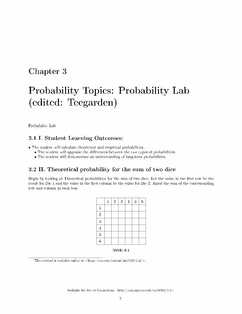
3.2 II. Theoretical probability for the sum of two dice

Begin by looking at Theoretical probabilities for the sum of two dice. Let the value in the �rst row be theresult for Die 1 and the value in the �rst column be the value for Die 2. Input the sum of the correspondingrow and column in each box.

+ 1 2 3 4 5 6

1

2

3

4

5

6

Table 3.1



7

8CHAPTER 3. PROBABILITY TOPICS: PROBABILITY LAB (EDITED:

TEEGARDEN)

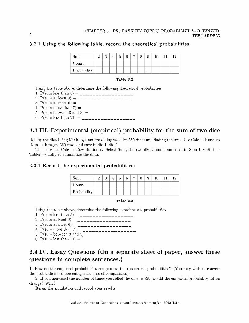
3.2.1 Using the following table, record the theoretical probabilities.

Sum 2 3 4 5 6 7 8 9 10 11 12

Count

Probability

Table 3.2

Using the table above, determine the following theoretical probabilities1. P(sum less than 5) = _________________2. P(sum at least 9) = _________________3. P(sum at most 6) = _________________4. P(sum more than 7) = _________________5. P(sum between 3 and 8) = _________________6. P(sum less than 11) = _________________

3.3 III. Experimental (empirical) probability for the sum of two dice

Rolling the dice Using Minitab, simulate rolling two dice 360 times and �nding the sum. Use Calc→ RandomData → Integer, 360 rows and save in die 1, die 2.

Then use the Calc → Row Statistics. Select Sum, the two die columns and save in Sum Use Stat →Tables → Tally to summarize the data.

3.3.1 Record the experimental probabilities:

Sum 2 3 4 5 6 7 8 9 10 11 12

Count

Probability

Table 3.3

Using the table above, determine the following experimental probabilities1. P(sum less than 5) = _________________2. P(sum at least 9) = _________________3. P(sum at most 6) = _________________4. P(sum more than 7) = _________________5. P(sum between 3 and 8) = _________________6. P(sum less than 11) = _________________

3.4 IV. Essay Questions (On a separate sheet of paper, answer thesequestions in complete sentences.)

1. How do the empirical probabilities compare to the theoretical probabilities? (You may wish to convertthe probabilities to percentages for ease of comparison.)

2. If you increased the number of times you rolled the dice to 720, would the empirical probability valueschange? Why?

Rerun the simulation and record your results.


9

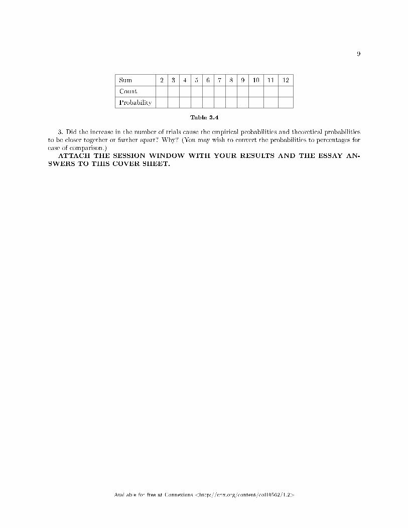
Sum 2 3 4 5 6 7 8 9 10 11 12

Count

Probability

Table 3.4

3. Did the increase in the number of trials cause the empirical probabilities and theoretical probabilitiesto be closer together or farther apart? Why? (You may wish to convert the probabilities to percentages forease of comparison.)

ATTACH THE SESSION WINDOW WITH YOUR RESULTS AND THE ESSAY AN-SWERS TO THIS COVER SHEET.


10CHAPTER 3. PROBABILITY TOPICS: PROBABILITY LAB (EDITED:

TEEGARDEN)


Chapter 4

Discrete Random Variables: Lab I(edited: Teegarden)1

Discrete Probability LabName:

4.1 Student Learning Outcomes:

• The student will compare empirical data and a theoretical distribution to determine if everyday exper-iment �ts a discrete distribution.

• The student will demonstrate an understanding of long-term probabilities.

Procedure: The experiment procedure is to pick one card from a deck of shu�ed cards.

1. The theoretical probability of picking a diamond from a deck is:2. Shu�e a deck of cards and pick one card from it and record whether it was a diamond or not a diamond.3. Put the card back and reshu�e.4. Do this a total of 10 times and record the number of diamonds picked.5. What is the experimental probability of drawing a diamond?6. How does the experimental probability compare to the theoretical probability? (high/low/about the

same)

Using Minitab, simulate this experiment (drawing a card 10 times and recording the number of diamonds)for a total of 50 times. Use Calc -> Random data -> Binomial.



11

12CHAPTER 4. DISCRETE RANDOM VARIABLES: LAB I (EDITED:

TEEGARDEN)

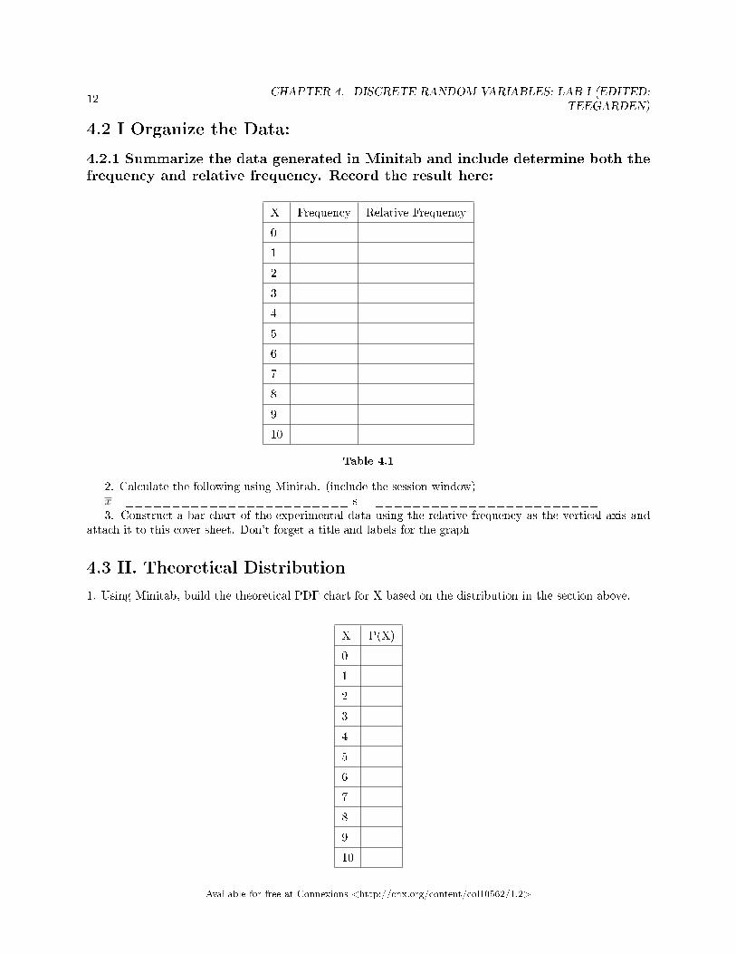
4.2 I Organize the Data:

4.2.1 Summarize the data generated in Minitab and include determine both the

frequency and relative frequency. Record the result here:

X Frequency Relative Frequency

0

1

2

3

4

5

6

7

8

9

10

Table 4.1

2. Calculate the following using Minitab. (include the session window)x= ________________________ s = ________________________3. Construct a bar chart of the experimental data using the relative frequency as the vertical axis and

attach it to this cover sheet. Don't forget a title and labels for the graph

4.3 II. Theoretical Distribution

1. Using Minitab, build the theoretical PDF chart for X based on the distribution in the section above.

X P(X)

0

1

2

3

4

5

6

7

8

9

10


13

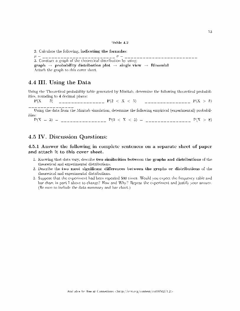
Table 4.2

2. Calculate the following, indicating the formulas:µ = ________________________ σ = ________________________3. Constuct a graph of the theoretical distribution by using:graph → probability distribution plot → single view → BinomialAttach the graph to this cover sheet.

4.4 III. Using the Data

Using the Theoretical probability table generated by Minitab, determine the following theoretical probabil-ities, rounding to 4 decimal places:

P(X = 3) =_______________ P(2 < X < 5) = _______________ P(X > 8)_______________

Using the data from the Minitab simulation, determine the following empirical (experimental) probabil-ities:

P(X = 3) = _______________ P(2 < X < 5) = _______________ P(X > 8)_______________

4.5 IV. Discussion Questions:

4.5.1 Answer the following in complete sentences on a separate sheet of paper

and attach it to this cover sheet.

1. Knowing that data vary, describe two similarities between the graphs and distributions of thetheoretical and experimental distributions.

2. Describe the two most signi�cant di�erences between the graphs or distributions of thetheoretical and experimental distributions.

3. Suppose that the experiment had been repeated 500 times. Would you expect the frequency table andbar chart in part I above to change? How and Why? Repeat the experiment and justify your answer.(Be sure to include the data summary and bar chart.)


14CHAPTER 4. DISCRETE RANDOM VARIABLES: LAB I (EDITED:

TEEGARDEN)


Chapter 5

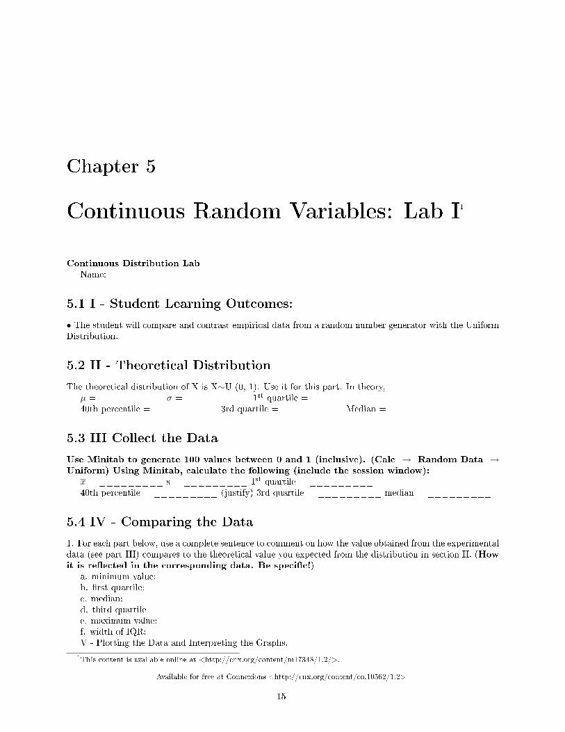
Continuous Random Variables: Lab I1

Continuous Distribution LabName:

5.1 I - Student Learning Outcomes:

• The student will compare and contrast empirical data from a random number generator with the UniformDistribution.

5.2 II - Theoretical Distribution

The theoretical distribution of X is X∼U (0, 1). Use it for this part. In theory,µ = _________ σ = _________ 1st quartile = _________40th percentile = _________ 3rd quartile = _________Median = _________

5.3 III Collect the Data

Use Minitab to generate 100 values between 0 and 1 (inclusive). (Calc → Random Data →Uniform) Using Minitab, calculate the following (include the session window):

x = _________ s = _________ 1st quartile = _________40th percentile = _________ (justify) 3rd quartile = _________ median = _________

5.4 IV - Comparing the Data

1. For each part below, use a complete sentence to comment on how the value obtained from the experimentaldata (see part III) compares to the theoretical value you expected from the distribution in section II. (Howit is re�ected in the corresponding data. Be speci�c!)

a. minimum value:b. �rst quartile:c. median:d. third quartilee. maximum value:f. width of IQR:V - Plotting the Data and Interpreting the Graphs.



15

16 CHAPTER 5. CONTINUOUS RANDOM VARIABLES: LAB I

1. What does the probability graph for the theoretical distribution look like? Draw it here and label theaxis.

2. Use Minitab to construct a histogram a using 5 bars and density as the y-axis value. Be sure to attachthe graphs to this lab.

a. Describe the shape of the histogram. Use 2 - 3 complete sentences. (Keep it simple. Does the graphgo straight across, does it have a V shape, does it have a hump in the middle or at either end, etc.? Oneway to help you determine the shape is to roughly draw a smooth curve through the top of the bars.)

b. How does this histogram compare to the graph of the theoretical uniform distribution? Draw thehorizontal line which represents the theoretical distribution on the histogram for ease of comparison. Besure to use 2 � 3 complete sentences.

3. Draw the box plot for the theoretical distribution and label the axis.4. Construct a box plot of the experimental data using Minitab and attach the graph.a. Do you notice any potential outliers? _________If so, which values are they? _________b. Numerically justify your answer using the appropriate formulas.c. How does this plot compare to the box plot of the theoretical uniform distribution? Be sure to use 2

� 3 complete sentences.

5.5 VI - Increasing the sample size. Repeat the simulation with 500data values.

1. Using Minitab, calculate the following (include the session window):x = _________ s = _________ 1st quartile = _________40th percentile = _________ (justify) 3rd quartile = _________ median = _________2. Does this data appear to re�ect the theoretical data more closely than the original? Be sure to use 2

� 3 complete sentences. (Be speci�c.)3. Create a histogram with 5 bars and using density for the y-axis and box plot for this data. (attach to

this lab)4. How do these compare to the theoretical distribution? Be sure to use 2 � 3 complete sentences. (Be

speci�c.)


Chapter 6

Normal Distribution: NormalDistribution Lab I (edited: Teegarden)1

Normal Distribution LabName:

6.1 I Student Learning Outcome:

* The student will compare and contrast empirical data and a theoretical distribution.* Find Probabilities for speci�c Normal Distributions

6.2 II The Situation

It is generally accepted that the mean body temperature is 98.6 degrees. If a sample of size 100 resulted ina sample mean of 98.3 degrees with a standard deviation of 0.64 degrees. Does this sample suggest that themean body temperature is actually lower than 98.6 degrees?

6.3 III Simulation: To answer the question, complete the followingsimulation.

Using Minitab (Calc -> Random Data-> Normal), generate 100 values from a normally distributed pop-ulation with a mean of 98.6 degrees and a standard deviation of 0.64 degrees (using the sample standarddeviation given in the situation since the population deviation is unknown). Repeat the simulation 9 moretimes for a total of 10. (Requesting the data be stored in c2-c10 will generate the remaining 9 columns ofdata with one command. )

6.4 IV Data Collection

Use Stats -> Basic Stats -> Display Descriptive and select all 10 columns to determine the sample mean foreach data set. Record the values below and include the session window with this lab.

x1 = _________ x2 = _________ x3 = _________ x4 = _________x5 = _________ x6 = _________ x7 = _________ x8 = _________x9 = _________ x10 = _________



17

18CHAPTER 6. NORMAL DISTRIBUTION: NORMAL DISTRIBUTION LAB I

(EDITED: TEEGARDEN)

6.5 V Analyze the Data � Using complete sentences.

Based on your simulation, do you think that a sample of size 100 with a mean temperature of 98.3 isreasonable? Answer using 2 � 3 complete sentences.

6.6 VI Finding Probabilities for Normal Distribution

For each of the following, �rst write the question in symbolic form and then using Minitab (Calc -> Probability Distributions -> Normal), �nd the probabilities. (attach your session window to thislab)_____________________

1. Given a population with a normal distribution, a mean of 0, and a standard deviation of 1, �nd theprobability of a value less than 1.25 _____________________

2. Given a population with a normal distribution, a mean of 25, and a standard deviation of 3, �nd theprobability of a value greater than 21.25._____________________

3. Given a population with a normal distribution, a mean of 100, and a standard deviation of 20, �ndthe probability of a value between 87 and 122._____________________

4. Given a population with a normal distribution, a mean of 150, and a standard deviation of 35, whatvalue has an area of 0.34 to the left?_____________________

5. Given a population with a normal distribution, a mean of 150, and a standard deviation of 35, whatvalue has an area of 0.34 to the right?_____________________

6. Given a population with a normal distribution, a mean of 15, and a standard deviation of 2, whatvalue has an area of 0.8 to the left?_____________________

7. Given a population with a normal distribution, a mean of 200, and a standard deviation of 15, whichtwo values form the upper and lower boundary of the middle 80%?___________________


Chapter 7

Central Limit Theorem: Central LimitTheorem Lab I (edited: Teegarden)1

Class Time:Name:


• The student will examine properties of the Central Limit Theorem.

7.2 Collect the Data

1. Using the random number generator in minitab, simulate the tossing of a single die 60 times. Calc ->Random Data -> Integer

2. Using Stat -> Tables -> Tally, summarize the data3. Construct a histogram using Minitab and then sketch the graph using a ruler and pencil. Scale the

axes.



19

20CHAPTER 7. CENTRAL LIMIT THEOREM: CENTRAL LIMIT THEOREM

LAB I (EDITED: TEEGARDEN)

Figure 7.1

4. Caluclate the following:

a. x =b. s =c. n = 1 (single die)

5. Draw a smooth curve through the tops of the bars of the histogram. Use 1 � 2 complete sentences todescribe the general shape of the curve.

7.3 Collecting Averages of Pairs

Repeat steps 1 - 5 (of the section above titled "Collect the Data") with one exception. Instead of recordingthe value of a single die, record the average of two dice. Use Minitab and generate 50 rows with two columns.Then use the Calc -> Row Statistics and select mean. Then use Stats -> Tables -> Tally to summarize thedata.

1. Construct a histogram. Scale the axes using the same scaling you did for the section titled "Collectingthe Data". Sketch the graph using a ruler and a pencil.


21

Figure 7.2

2. Calculate the following:

a. x =b. s =c. n = 2 (surveying one person at a time)

3. Draw a smooth curve through tops of the bars of the histogram. Use 1 � 2 complete sentences todescribe the general shape of the curve.

7.4 Collecting Averages of Groups of Five

Repeat steps 1 � 5 (of part I) with one exception. Instead of recording the value for a single die, record theaverage value for each of the 50 groups of 5 die tosses.

1. Generate �fty groups of 5 die tosses. Record the values of the average of their value.2. Construct a histogram. Scale the axes using the same scaling you did for section titled "Collect the

Data". Sketch the graph using a ruler and a pencil.




Figure 7.3


a. x =b. s =c. n = 5 (surveying �ve people at a time)

4. Draw a smooth curve through tops of the bars of the histogram. Use 1 � 2 complete sentences todescribe the general shape of the curve.

7.5 Collecting Averages of Groups of 20

Repeat steps 1 � 5 (of part I) recording the average value for each of the 50 groups of 20 die tosses.

1. Generate �fty groups of 20 die tosses. Record the values of the average of their value.2. Construct a histogram. Scale the axes using the same scaling you did for section titled "Collect the

Data". Sketch the graph using a ruler and a pencil.


23

Figure 7.4

3. Calculate the following4. Draw a smooth curve through tops of the bars of the histogram. Use 1 � 2 complete sentences to

describe the general shape of the curve.

7.6 Discussion Questions

1. As n changed, why did the shape of the distribution of the data change? Use 1 � 2 complete sentencesto explain what happened.

2. In the section titled "Collect the Data", what was the approximate distribution of the data? X ∼3. In the section titled "Collecting Averages of Groups of Five", what was the approximate distribution

of the data? X ∼4. In the section titled "Collecting Averages of Groups of Twenty", what was the approximate distribution

of the data? X ∼5. In 1 � 2 complete sentences, explain any di�erences in your answers to previous three questions.





Chapter 8

Con�dence Intervals: Con�denceInterval Lab I (edited: Teegarden)1

Class Time:Name:


• The student will calculate the 90% con�dence interval for the average cost of a home in the area inwhich this school is located.

• The student will interpret con�dence intervals.• The student will examine the e�ects that changing conditions has on the con�dence interval.


Check the Real Estate section in your local newspaper or website. (Note: many papers only list them oneday per week. Also, we will assume that homes come up for sale randomly.) Record the sales prices for 35randomly selected homes recently listed in the county.

1. Complete the table:

__________ __________ __________ __________ __________

__________ __________ __________ __________ __________

__________ __________ __________ __________ __________

__________ __________ __________ __________ __________

__________ __________ __________ __________ __________

__________ __________ __________ __________ __________

__________ __________ __________ __________ __________

Table 8.1



25

26CHAPTER 8. CONFIDENCE INTERVALS: CONFIDENCE INTERVAL LAB I

(EDITED: TEEGARDEN)

8.3 Describe the Data

1. Compute the following:

a. x =b. sx =c. n =

2. De�ne the Random Variable X, in words. X =3. State the estimated distribution to use. Use both words and symbols.

8.4 Find the Con�dence Interval

1. Calculate the con�dence interval and the error bound.

a. Con�dence Interval:b. Error Bound:

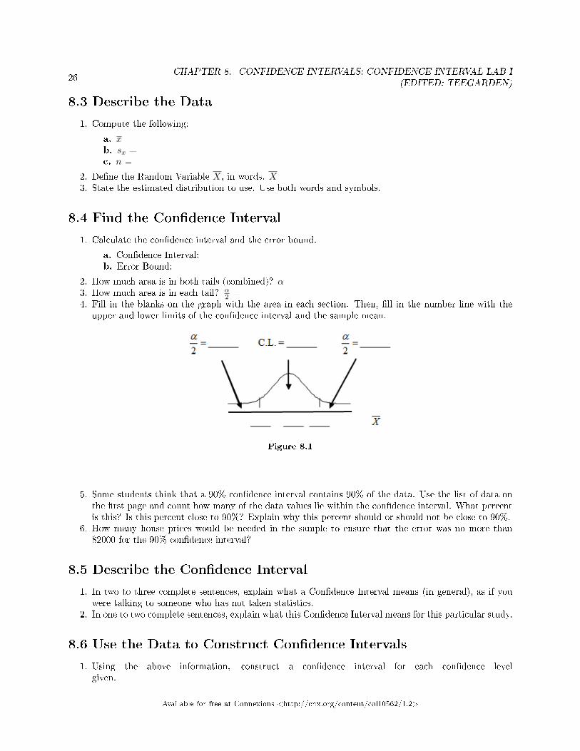
2. How much area is in both tails (combined)? α =3. How much area is in each tail? α

2 =4. Fill in the blanks on the graph with the area in each section. Then, �ll in the number line with the

upper and lower limits of the con�dence interval and the sample mean.

Figure 8.1

5. Some students think that a 90% con�dence interval contains 90% of the data. Use the list of data onthe �rst page and count how many of the data values lie within the con�dence interval. What percentis this? Is this percent close to 90%? Explain why this percent should or should not be close to 90%.

6. How many house prices would be needed in the sample to ensure that the error was no more than$2000 for the 90% con�dence interval?

8.5 Describe the Con�dence Interval

1. In two to three complete sentences, explain what a Con�dence Interval means (in general), as if youwere talking to someone who has not taken statistics.

2. In one to two complete sentences, explain what this Con�dence Interval means for this particular study.

8.6 Use the Data to Construct Con�dence Intervals

1. Using the above information, construct a con�dence interval for each con�dence levelgiven.


27

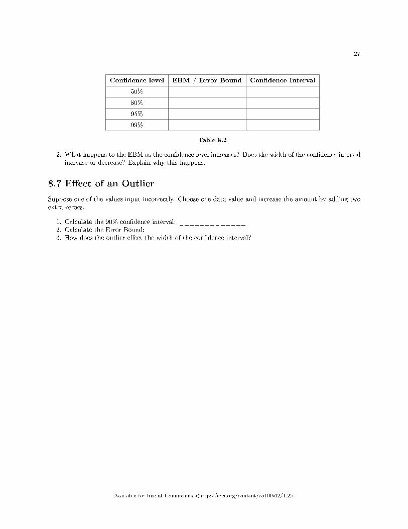
Con�dence level EBM / Error Bound Con�dence Interval

50%

80%

95%

99%

Table 8.2

2. What happens to the EBM as the con�dence level increases? Does the width of the con�dence intervalincrease or decrease? Explain why this happens.

8.7 E�ect of an Outlier

Suppose one of the values input incorrectly. Choose one data value and increase the amount by adding twoextra zeroes.

1. Calculate the 90% con�dence interval: _____________2. Calculate the Error Bound: ____________3. How does the outlier e�ect the width of the con�dence interval?


28CHAPTER 8. CONFIDENCE INTERVALS: CONFIDENCE INTERVAL LAB I

(EDITED: TEEGARDEN)


Chapter 9

Con�dence Intervals: Con�denceInterval Lab II (edited: Teegarden)1

Class Time:Name:


• The student will calculate the 90% con�dence interval for proportion of students in this school thatwere born in this state.

• The student will interpret con�dence intervals.• The student will examine the e�ects that changing conditions has on the con�dence interval.


1. Survey the students in your class, asking them if they were born in this state. Let X = the numberthat were born in this state.

a. n =____________b. x =____________

2. De�ne the Random Variable P ' in words.3. State the estimated distribution to use.

9.3 Find the Con�dence Interval and Error Bound

1. Calculate the con�dence interval and the error bound.

a. Con�dence Interval:b. Error Bound:

2. How much area is in both tails (combined)? α=3. How much area is in each tail? α

2 =4. Fill in the blanks on the graph with the area in each section. Then, �ll in the number line with the

upper and lower limits of the con�dence interval and the sample proportion.



29

30CHAPTER 9. CONFIDENCE INTERVALS: CONFIDENCE INTERVAL LAB

II (EDITED: TEEGARDEN)

Figure 9.1

5. How large a sample would be needed to ensure that the error for the 90% con�dence interval is only5%? Use the previous data as an estimate for p.

6. Recalculate the sample size assuming there is no previous data.

9.4 Describe the Con�dence Interval

1. In two to three complete sentences, explain what a Con�dence Interval means (in general), as if youwere talking to someone who has not taken statistics.

2. In one to two complete sentences, explain what this Con�dence Interval means for this particular study.3. Using the above information, construct a con�dence interval for each given con�dence level

given.

Con�dence level EBP / Error Bound Con�dence Interval

50%

80%

95%

99%

Table 9.1

4. What happens to the EBP as the con�dence level increases? Does the width of the con�dence intervalincrease or decrease? Explain why this happens.


Chapter 10

Con�dence Intervals: Con�denceInterval Lab III (edited: Teegarden)1

Class Time:Name:


• The student will calculate a 90% con�dence interval using the given data.• The student will examine the relationship between the con�dence level and the percent of constructed

intervals that contain the population average.



31


III (EDITED: TEEGARDEN)

10.2 Given:

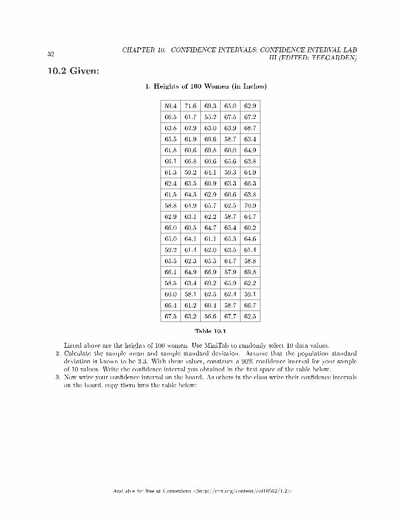
1. Heights of 100 Women (in Inches)

59.4 71.6 69.3 65.0 62.9

66.5 61.7 55.2 67.5 67.2

63.8 62.9 63.0 63.9 68.7

65.5 61.9 69.6 58.7 63.4

61.8 60.6 69.8 60.0 64.9

66.1 66.8 60.6 65.6 63.8

61.3 59.2 64.1 59.3 64.9

62.4 63.5 60.9 63.3 66.3

61.5 64.3 62.9 60.6 63.8

58.8 64.9 65.7 62.5 70.9

62.9 63.1 62.2 58.7 64.7

66.0 60.5 64.7 65.4 60.2

65.0 64.1 61.1 65.3 64.6

59.2 61.4 62.0 63.5 61.4

65.5 62.3 65.5 64.7 58.8

66.1 64.9 66.9 57.9 69.8

58.5 63.4 69.2 65.9 62.2

60.0 58.1 62.5 62.4 59.1

66.4 61.2 60.4 58.7 66.7

67.5 63.2 56.6 67.7 62.5

Table 10.1

Listed above are the heights of 100 women. Use MiniTab to randomly select 10 data values.2. Calculate the sample mean and sample standard deviation. Assume that the population standard

deviation is known to be 3.3. With these values, construct a 90% con�dence interval for your sampleof 10 values. Write the con�dence interval you obtained in the �rst space of the table below.

3. Now write your con�dence interval on the board. As others in the class write their con�dence intervalson the board, copy them into the table below:


33

90% Con�dence Intervals

__________ __________ __________ __________ __________

__________ __________ __________ __________ __________

__________ __________ __________ __________ __________

__________ __________ __________ __________ __________

__________ __________ __________ __________ __________

__________ __________ __________ __________ __________

__________ __________ __________ __________ __________

__________ __________ __________ __________ __________

Table 10.2


1. The actual population mean for the 100 heights given above is µ = 63.4. Using the class listing ofcon�dence intervals, count how many of them contain the population mean µ; i.e., for how manyintervals does the value of µ lie between the endpoints of the con�dence interval?

2. Divide this number by the total number of con�dence intervals generated by the class to determine thepercent of con�dence intervals that contain the mean µ. Write this percent below.

3. Is the percent of con�dence intervals that contain the population mean µ close to 90%?4. Suppose we had generated 100 con�dence intervals. What do you think would happen to the percent

of con�dence intervals that contained the population mean?5. When we construct a 90% con�dence interval, we say that we are 90% con�dent that the truepopulation mean lies within the con�dence interval. Using complete sentences, explain whatwe mean by this phrase.

6. Some students think that a 90% con�dence interval contains 90% of the data. Use the list of data givenon the �rst page and count how many of the data values lie within the con�dence interval that yougenerated on that page. How many of the 100 data values lie within your con�dence interval? Whatpercent is this? Is this percent close to 90%?

7. Explain why it does not make sense to count data values that lie in a con�dence interval. Think aboutthe random variable that is being used in the problem.

8. Suppose you obtained the heights of 10 women and calculated a con�dence interval from this informa-tion. Without knowing the population mean µ, would you have any way of knowing for certain ifyour interval actually contained the value of µ? Explain.

note: This lab was designed and contributed by Diane Mathios.



III (EDITED: TEEGARDEN)


Chapter 11

Hypothesis Testing of Single Mean andSingle Proportion: Lab (Edited:Teegarden) 021

Class Time:Name:


• The student will select the appropriate distributions to use in each case.• The student will conduct hypothesis tests and interpret the results.

11.2 Television Survey

The data in the Testbook.mtw �le lists the cost of 62 books required for classes in Summer 2008 at MesaCollege. Students believe that they are spending on average $100 for their textbooks. Using the data fornew books as the sample, conduct a hypothesis test to determine if the average cost of new textbooks atMesa is lower.

1. Ho:2. Ha:3. In words, de�ne the random variable. __________ =4. The distribution to use for the test is:5. Calculate the test statistic using your data.6. Draw a graph and label it appropriately.

a. Graph:



35

36CHAPTER 11. HYPOTHESIS TESTING OF SINGLE MEAN AND SINGLE

PROPORTION: LAB (EDITED: TEEGARDEN) 02

Figure 11.1

b. Calculate the p-value:

7. Do you or do you not reject the null hypothesis? Why?8. Write a clear conclusion using a complete sentence.

11.3 Language Survey

According to the 2000 Census, about 39.5% of Californians and 17.9% of all Americans speak a languageother than English at home. Using your class as the sample, conduct a hypothesis test to determine if thepercent of the students at your school that speak a language other than English at home is di�erent from39.5%.

1. Ho:2. Ha:3. In words, de�ne the random variable. __________ =4. The distribution to use for the test is:5. Calculate the test statistic using your data.6. Draw a graph and label it appropriately. Shade the actual level of signi�cance.

a. Graph:


37

Figure 11.2


7. Do you or do you not reject the null hypothesis? Why?8. Write a clear conclusion using a complete sentence.


38CHAPTER 11. HYPOTHESIS TESTING OF SINGLE MEAN AND SINGLE

PROPORTION: LAB (EDITED: TEEGARDEN) 02


Chapter 12

Hypothesis Testing of Two Means andTwo Proportions: Lab I (edited:Teegarden 02)1

Class Time:Name:


• The student will select the appropriate distributions to use in each case.• The student will conduct hypothesis tests and interpret the results.

12.2 Increasing Stocks Survey

Look at yesterday's newspaper business section. Conduct a hypothesis test to determine if the proportion ofNew York Stock Exchange (NYSE) stocks that increased is greater than the proportion of NASDAQ stocksthat increased. As randomly as possible, choose 40 NYSE stocks and 32 NASDAQ stocks and input thedata into a Minitab worksheet. Complete the following statements.

1. Ho

2. Ha

3. In words, de�ne the Random Variable. ____________=4. The distribution to use for the test is:5. Calculate the test statistic using your data.6. Draw a graph and label it appropriately. Shade the actual level of signi�cance.

a. Graph:



39

40CHAPTER 12. HYPOTHESIS TESTING OF TWO MEANS AND TWO

PROPORTIONS: LAB I (EDITED: TEEGARDEN 02)

Figure 12.1


7. Do you reject or not reject the null hypothesis? Why?8. Write a clear conclusion using a complete sentence.

12.3 Textbook Prices

The data in Textbook.mtw shows the price for both the new and used textbook price for books required forsummer 2008 classes at Mesa College. Is it worthwhile to buy used textbooks?

1. Ho

2. Ha


a. Graph:


41

Figure 12.2



12.4 Shoe Survey

Test whether women have, on average, more pairs of shoes than men. Include all forms of sneakers, shoes,sandals, and boots. Use your class as the sample.

1. Ho

2. Ha


a. Graph:


42CHAPTER 12. HYPOTHESIS TESTING OF TWO MEANS AND TWO

PROPORTIONS: LAB I (EDITED: TEEGARDEN 02)

Figure 12.3




Chapter 13

The Chi-Square Distribution: Lab I(edited: Teegarden)1

Class Time:Name:

13.1 Student Learning Outcome:

• The student will evaluate data collected to determine if they �t either a uniform distribution.


Three car-pooling students claimed that they missed their statistics test because they had a �at tire. On themake-up test the instructor asked them to identify the particular tire that went �at. The instructor assumedthat the distribution would be uniform. To test this assumption,survey the class to determine the numberthe which tire they would select.

Tire Left Front Left Rear Right Front Right Rear

Number Selected

Table 13.1

13.3 Hypothesis Test

Conduct a hypothesis test to determine if the selection of a tire �ts a Uniform Distribution.

1. Ho:2. Ha:3. Calculate the test statistic.4. Find the p-value.5. Sketch a graph of the situation. Label and scale the x-axis. Shade the area corresponding to the

p-value.



43

44CHAPTER 13. THE CHI-SQUARE DISTRIBUTION: LAB I (EDITED:

TEEGARDEN)

Figure 13.1

6. State your decision.7. State your conclusion in a complete sentence.8. If in fact the students did not have a �at tire, do you think they will be caught out? Explain.


Chapter 14

The Chi-Square Distribution: Lab II(edited: Teegarden)1

Class Time:Name:

14.1 Student Learning Outcome:

• The student will evaluate if there is a signi�cant relationship between favorite type of snack and gender.


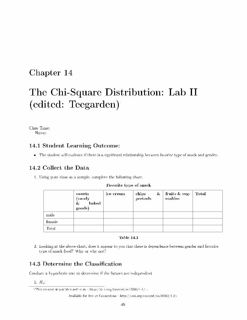
1. Using your class as a sample, complete the following chart.

Favorite type of snack

sweets(candy& bakedgoods)

ice cream chips &pretzels

fruits & veg-etables

Total

male

female

Total

Table 14.1

2. Looking at the above chart, does it appear to you that there is dependence between gender and favoritetype of snack food? Why or why not?

14.3 Determine the Classi�cation

Conduct a hypothesis test to determine if the factors are independent

1. Ho:



45

46CHAPTER 14. THE CHI-SQUARE DISTRIBUTION: LAB II (EDITED:

TEEGARDEN)

2. Ha:3. What distribution should you use for a hypothesis test?4. Why did you choose this distribution?5. Calculate the test statistic.6. Find the p-value.7. Sketch a graph of the situation. Label and scale the x-axis. Shade the area corresponding to the

p-value.

Figure 14.1

8. State your decision.9. State your conclusion in a complete sentence.


1. Is the conclusion of your study the same as or di�erent from your answer to (I2) above?2. Why do you think that occurred?


Chapter 15

Linear Regression and Correlation:Regression Lab II (edited: Teegarden)1

Class Time:Name:


• The student will calculate and construct the line of best �t between two variables.• The student will evaluate the relationship between two variables to determine if that relationship is

signi�cant.


Survey 10 textbooks. Collect bivariate data (number of pages in a textbook, the cost of the textbook).

1. Complete the table.



47

48CHAPTER 15. LINEAR REGRESSION AND CORRELATION: REGRESSION

LAB II (EDITED: TEEGARDEN)

Number of pages Cost of textbook

Figure 15.1

2. Which variable should be the dependent variable and which should be the independent variable? Why?3. Graph �number of pages� vs. �cost.� Plot the points on the graph. Label both axes with words. Scale

both axes.


49

Figure 15.2

Does there appear to be a relationship between the size of the book and it's cost?

15.3 Analyze the Data

Enter your data into your MiniTab. Record the following information.

1. correlation coe�cient = ___________2. p-value = ___________3. Is three signi�cant correlation to use a regression line?


a. a =b. b =c. n =d. equation: y =

2. Obtain the graph using Minitab. Sketch the regression line below.


50CHAPTER 15. LINEAR REGRESSION AND CORRELATION: REGRESSION

LAB II (EDITED: TEEGARDEN)

Figure 15.3

3. Supply an answer for the following senarios:

a. For a textbook with 400 pages, predict the cost:b. For a textbook with 600 pages, predict the cost:


1. Answer each with 1-3 complete sentences.

a. Does the line seem to �t the data? Why?b. What does the correlation imply about the relationship between the number of pages and the

cost?

2. Are there any outliers? If so, which point(s) is an outlier?3. Should the outlier, if it exists, be removed? Why or why not?


Chapter 16

Collaborative Statistics: Group Project -Teegarden1

16.1 Student Learning Objectives

• The student will identify a hypothesis testing problem in print.• The student will conduct a survey to verify or dispute the results of the hypothesis test.• The student will summarize the article, analysis, and conclusions in a report.

16.2 Instructions

As you complete each task below, check it o�. Answer all questions in your summary. This project may bedone in pairs or a group of three. Be sure to ensure that all the students participate equally in the work.This project is worth 20% of your �nal grade.

____ Find an article in a newspaper, magazine or on the internet which makes a claim aboutONE population mean or ONE population proportion. The claim may be based upon a surveythat the article was reporting on. Decide whether this claim is the null or alternate hypothesis.

____ Copy or print out the article and include a copy in your project, along with the source.____ State how you will collect your data. (Convenience sampling is not acceptable.)____ Conduct your survey. You must have more than 50 responses in your sample.

When you hand in your �nal project, attach the tally sheet or the packet of questionnaires thatyou used to collect data. Your data must be real.

____ State the statistics that are a result of your data collection: sample size, sample mean, andsample standard deviation, OR sample size and number of successes.

____ Make 2 copies of the appropriate solution sheet.____ Record the hypothesis test on the solution sheet, based on your experiment. Do a

DRAFT solution �rst on one of the solution sheets and check it over carefully. Have a classmatecheck your solution to see if it is done correctly. Make your decision using a 5% level of signi�cance.Include the 95% con�dence interval on the solution sheet.

____ Create at least two di�erent graphs to illustrate your data. This may be a pie or barchart or may be a histogram or box plot, depending on the nature of your data. Produce graphsthat makes sense for your data and gives useful visual information about your data. Include ananalysis of the graphs in your summary.



51

52CHAPTER 16. COLLABORATIVE STATISTICS: GROUP PROJECT -

TEEGARDEN

____ Write your summary (in complete sentences and paragraphs, with proper grammar andcorrect spelling) that describes the project. The summary MUST include:

1. Brief discussion of the article, including the source.2. Statement of the claim made in the article (one of the hypotheses).3. Detailed description of how, where, and when you collected the data, including the sampling

technique. Did you use cluster, strati�ed, systematic, or simple random sampling (using arandom number generator)? As stated above, convenience sampling is not acceptable.

4. Discuss the shape of your data and the relevant inforamition obtained from your graphs.5. Conclusion about the article claim in light of your hypothesis test. This is the conclusion

of your hypothesis test, stated in words, in the context of the situation in your project insentence form, as if you were writing this conclusion for a non-statistician.

6. Sentence interpreting your con�dence interval in the context of the situation in your project.

16.3 Assignment Checklist

Turn in the following typed (12 point) and stapled packet for your �nal project:

____ Cover sheet containing your name(s), class time, and the name of your study.____ Summary, which includes all items listed on summary checklist.____ Solution sheet neatly and completely �lled out. The solution sheet does not need to be

typed.____ Graphic representation of your data, created following the guidelines discussed above.

Include only graphs which are appropriate and useful.____ Raw data collected AND a table summarizing the sample data (n, xbar and s; or

x, n, and p', as appropriate for your hypotheses). The raw data does not need to be typed, butthe summary does. Hand in the data as you collected it. (Either attach your tally sheet or anenvelope containing your questionnaires.)


INDEX 53

Index of Keywords and Terms

Keywords are listed by the section with that keyword (page numbers are in parentheses). Keywordsdo not necessarily appear in the text of the page. They are merely associated with that section. Ex.apples, � 1.1 (1) Terms are referenced by the page they appear on. Ex. apples, 1

A article, � 16(51)

B box, � 5(15)

C cards, � 4(11)continuous, � 5(15)cumulative, � 1(1)

D data, � 1(1)discrete, � 4(11)distribution, � 4(11), � 5(15)

E elementary, � 2(5), � 3(7), � 4(11), � 5(15),� 6(17), � 7(19), � 8(25), � 9(29), � 10(31),� 11(35), � 12(39), � 13(43), � 14(45), � 15(47),� 16(51)empirical, � 5(15)exercise, � 3(7), � 4(11), � 5(15)experiment, � 4(11)

F frequency, � 1(1)

H histogram, � 5(15)homework, � 3(7), � 4(11)

hypothesis, � 16(51)

L lab, � 3(7), � 4(11), � 5(15)long-term, � 3(7)

P plot, � 5(15)probability, � 3(7), � 4(11)

R random, � 4(11)relative, � 1(1)replacement, � 3(7)

S sampling, � 1(1)statistics, � 1(1), � 2(5), � 3(7), � 4(11),� 5(15), � 6(17), � 7(19), � 8(25), � 9(29),� 10(31), � 11(35), � 12(39), � 13(43), � 14(45),� 15(47), � 16(51)survey, � 16(51)systematic, � 1(1)

T test, � 16(51)

U uniform, � 5(15)

V variable, � 4(11)


54 ATTRIBUTIONS

Attributions

Collection: Labs For Collaborative Statistics - TeegardenEdited by: Mary TeegardenURL: http://cnx.org/content/col10562/1.2/License: http://creativecommons.org/licenses/by/2.0/

Module: "Candy Lab"By: Mary TeegardenURL: http://cnx.org/content/m17323/1.2/Pages: 1-3Copyright: Mary TeegardenLicense: http://creativecommons.org/licenses/by/2.0/Based on: Sampling and Data: Data Collection Lab IBy: Barbara Illowsky, Ph.D., Susan DeanURL: http://cnx.org/content/m16004/1.8/

Module: "Descriptive Statistics: Descriptive Statistics Lab (edited: Teegarden)"By: Mary TeegardenURL: http://cnx.org/content/m17333/1.2/Pages: 5-6Copyright: Mary TeegardenLicense: http://creativecommons.org/licenses/by/2.0/Based on: Descriptive Statistics: Descriptive Statistics LabBy: Barbara Illowsky, Ph.D., Susan DeanURL: http://cnx.org/content/m16299/1.7/

Module: "Probability Topics: Probability Lab (edited: Teegarden)"By: Mary TeegardenURL: http://cnx.org/content/m17335/1.2/Pages: 7-9Copyright: Mary TeegardenLicense: http://creativecommons.org/licenses/by/2.0/Based on: Probability Topics: Probability LabBy: Barbara Illowsky, Ph.D., Susan DeanURL: http://cnx.org/content/m16841/1.5/

Module: "Discrete Random Variables: Lab I (edited: Teegarden)"By: Mary TeegardenURL: http://cnx.org/content/m17336/1.2/Pages: 11-13Copyright: Mary TeegardenLicense: http://creativecommons.org/licenses/by/2.0/Based on: Discrete Random Variables: Lab IBy: Barbara Illowsky, Ph.D., Susan DeanURL: http://cnx.org/content/m16827/1.5/


ATTRIBUTIONS 55

Module: "Continuous Random Variables: Lab I"By: Mary TeegardenURL: http://cnx.org/content/m17348/1.2/Pages: 15-16Copyright: Mary TeegardenLicense: http://creativecommons.org/licenses/by/2.0/Based on: Continuous Random Variables: Lab IBy: Barbara Illowsky, Ph.D., Susan DeanURL: http://cnx.org/content/m16803/1.5/

Module: "Normal Distribution: Normal Distribution Lab I (edited: Teegarden)"By: Mary TeegardenURL: http://cnx.org/content/m17338/1.3/Pages: 17-18Copyright: Mary TeegardenLicense: http://creativecommons.org/licenses/by/2.0/Based on: Normal Distribution: Normal Distribution Lab IBy: Barbara Illowsky, Ph.D., Susan DeanURL: http://cnx.org/content/m16981/1.7/

Module: "Central Limit Theorem: Central Limit Theorem Lab I (edited: Teegarden)"By: Mary TeegardenURL: http://cnx.org/content/m17339/1.1/Pages: 19-23Copyright: Mary TeegardenLicense: http://creativecommons.org/licenses/by/2.0/Based on: Central Limit Theorem: Central Limit Theorem Lab IBy: Barbara Illowsky, Ph.D., Susan DeanURL: http://cnx.org/content/m16950/1.5/

Module: "Con�dence Intervals: Con�dence Interval Lab I (edited: Teegarden)"By: Mary TeegardenURL: http://cnx.org/content/m17340/1.1/Pages: 25-27Copyright: Mary TeegardenLicense: http://creativecommons.org/licenses/by/2.0/Based on: Con�dence Intervals: Con�dence Interval Lab IBy: Barbara Illowsky, Ph.D., Susan DeanURL: http://cnx.org/content/m16960/1.5/

Module: "Con�dence Intervals: Con�dence Interval Lab II (edited: Teegarden)"By: Mary TeegardenURL: http://cnx.org/content/m17341/1.1/Pages: 29-30Copyright: Mary TeegardenLicense: http://creativecommons.org/licenses/by/2.0/Based on: Con�dence Intervals: Con�dence Interval Lab IIBy: Barbara Illowsky, Ph.D., Susan DeanURL: http://cnx.org/content/m16961/1.5/


56 ATTRIBUTIONS

Module: "Con�dence Intervals: Con�dence Interval Lab III (edited: Teegarden)"By: Mary TeegardenURL: http://cnx.org/content/m17342/1.1/Pages: 31-33Copyright: Mary TeegardenLicense: http://creativecommons.org/licenses/by/2.0/Based on: Con�dence Intervals: Con�dence Interval Lab IIIBy: Barbara Illowsky, Ph.D., Susan DeanURL: http://cnx.org/content/m16964/1.5/

Module: "Hypothesis Testing of Single Mean and Single Proportion: Lab (Edited: Teegarden) 02"By: Mary TeegardenURL: http://cnx.org/content/m17354/1.1/Pages: 35-37Copyright: Mary TeegardenLicense: http://creativecommons.org/licenses/by/2.0/Based on: Hypothesis Testing of Single Mean and Single Proportion: Lab (Edited: Teegarden) 02By: Barbara Illowsky, Ph.D., Susan Dean, Mary TeegardenURL: http://cnx.org/content/m17351/1.1/

Module: "Hypothesis Testing of Two Means and Two Proportions: Lab I (edited: Teegarden 02)"By: Mary TeegardenURL: http://cnx.org/content/m17350/1.2/Pages: 39-42Copyright: Mary TeegardenLicense: http://creativecommons.org/licenses/by/2.0/Based on: Hypothesis Testing of Two Means and Two Proportions: Lab IBy: Barbara Illowsky, Ph.D., Susan DeanURL: http://cnx.org/content/m17022/1.6/

Module: "The Chi-Square Distribution: Lab I (edited: Teegarden)"By: Mary TeegardenURL: http://cnx.org/content/m17328/1.1/Pages: 43-44Copyright: Mary TeegardenLicense: http://creativecommons.org/licenses/by/2.0/Based on: The Chi-Square Distribution: Lab IBy: Barbara Illowsky, Ph.D., Susan DeanURL: http://cnx.org/content/m17049/1.4/

Module: "The Chi-Square Distribution: Lab II (edited: Teegarden)"By: Mary TeegardenURL: http://cnx.org/content/m17330/1.1/Pages: 45-46Copyright: Mary TeegardenLicense: http://creativecommons.org/licenses/by/2.0/Based on: The Chi-Square Distribution: Lab IIBy: Barbara Illowsky, Ph.D., Susan DeanURL: http://cnx.org/content/m17050/1.5/


ATTRIBUTIONS 57

Module: "Linear Regression and Correlation: Regression Lab II (edited: Teegarden)"By: Mary TeegardenURL: http://cnx.org/content/m17331/1.1/Pages: 47-50Copyright: Mary TeegardenLicense: http://creativecommons.org/licenses/by/2.0/Based on: Linear Regression and Correlation: Regression Lab IIBy: Barbara Illowsky, Ph.D., Susan DeanURL: http://cnx.org/content/m17087/1.4/

Module: "Collaborative Statistics: Group Project - Teegarden"By: Mary TeegardenURL: http://cnx.org/content/m17356/1.1/Pages: 51-52Copyright: Mary TeegardenLicense: http://creativecommons.org/licenses/by/2.0/Based on: Collaborative Statistics: Projects: Hypothesis Testing ArticleBy: Barbara Illowsky, Ph.D., Susan DeanURL: http://cnx.org/content/m17140/1.5/


Labs For Collaborative Statistics - TeegardenThis is a collection of labs from Collaborative Statistics by Illowski and Dean which have been edited toinclude Minitab activities. In addition the labs are to be done as individual activities.

About ConnexionsSince 1999, Connexions has been pioneering a global system where anyone can create course materials andmake them fully accessible and easily reusable free of charge. We are a Web-based authoring, teaching andlearning environment open to anyone interested in education, including students, teachers, professors andlifelong learners. We connect ideas and facilitate educational communities.

Connexions's modular, interactive courses are in use worldwide by universities, community colleges, K-12schools, distance learners, and lifelong learners. Connexions materials are in many languages, includingEnglish, Spanish, Chinese, Japanese, Italian, Vietnamese, French, Portuguese, and Thai. Connexions is partof an exciting new information distribution system that allows for Print on Demand Books. Connexionshas partnered with innovative on-demand publisher QOOP to accelerate the delivery of printed coursematerials and textbooks into classrooms worldwide at lower prices than traditional academic publishers.

Documents

Labs For Collaborative Statistics - Teegarden2.2.pdf... · Chapter 1 Candy Lab 1 Candy Lab Name: 1.1 Student Learning Outcomes The student will construct Relative requencyF ables.T