AOE 5204

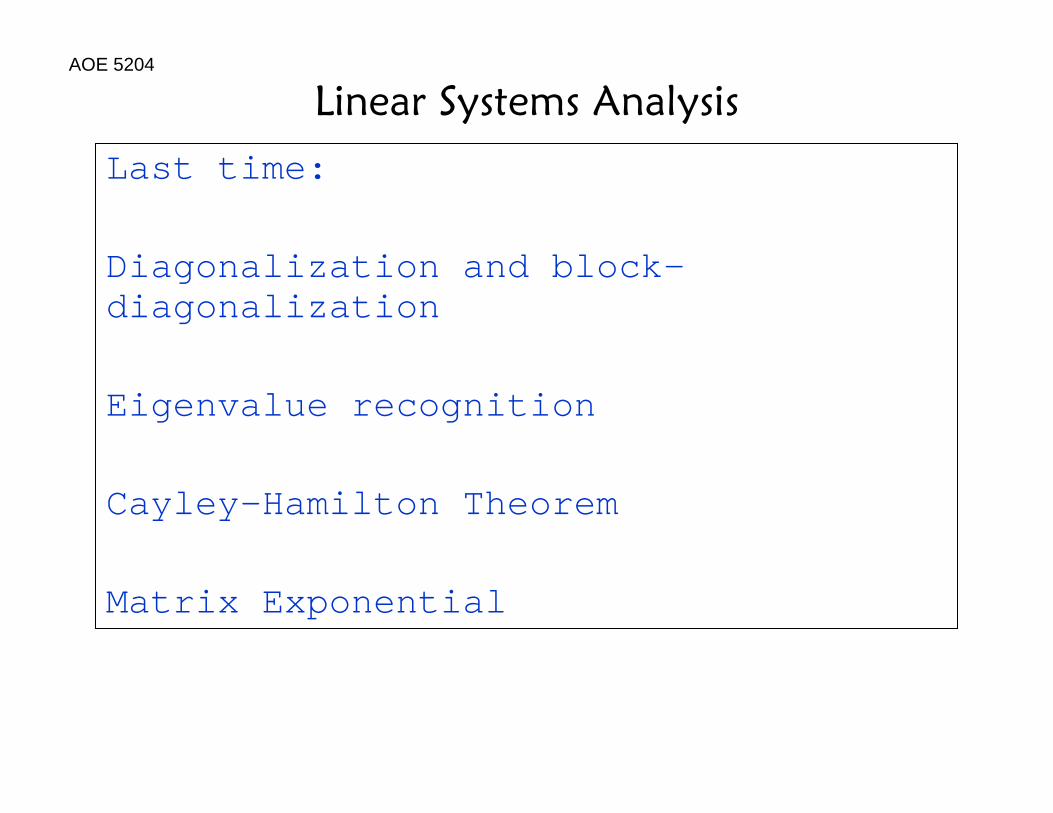
Linear Systems AnalysisLast time:

Diagonalization and block-diagonalization

Eigenvalue recognition

Cayley-Hamilton Theorem

Matrix Exponential

AOE 5204

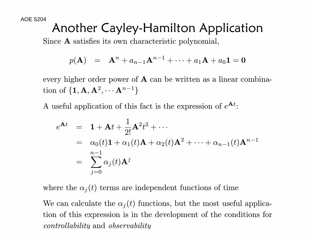
Another Cayley-Hamilton ApplicationSince A satisfies its own characteristic polynomial,

p(A) = An + an−1An−1 + · · ·+ a1A+ a01 = 0

every higher order power of A can be written as a linear combina-

tion of {1,A,A2, · · ·An−1}

A useful application of this fact is the expression of eAt:

eAt = 1+At+1

2!A2t2 + · · ·

= α0(t)1+ α1(t)A+ α2(t)A2 + · · ·+ αn−1(t)A

n−1

=n−1Xj=0

αj(t)Aj

where the αj(t) terms are independent functions of time

We can calculate the αj(t) functions, but the most useful applica-

tion of this expression is in the development of the conditions for

controllability and observability

AOE 5204

Modal AnalysisWe have already seen the modal decomposition that arises when

we diagonalize or block-diagonalize a linear system

A more detailed example:

A =

⎡⎣ 4 −6 −12 −1 −14 −4 −4

⎤⎦has eigenvalues (−3.6252, 1.3126 ± i1.9478) (stable or unstable?),and eigenvectors

E =

⎡⎣ 0.2565 −0.8154 −0.81540.1673 −0.2967 + i0.2740 −0.2967− i0.27400.9520 −0.4109− i0.0556 −0.4109 + i0.0556

⎤⎦Block-diagonalize by defining

Eb = [e1 Re{e2} Im{e2}] and Λb = E−1b AEb

AOE 5204

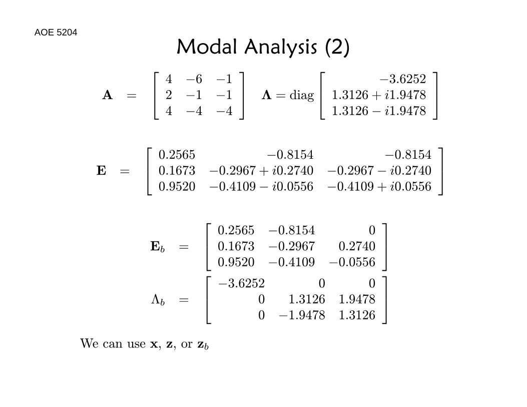
Modal Analysis (2)

A =

⎡⎣ 4 −6 −12 −1 −14 −4 −4

⎤⎦ Λ = diag

⎡⎣ −3.62521.3126 + i1.94781.3126− i1.9478

⎤⎦

E =

⎡⎣ 0.2565 −0.8154 −0.81540.1673 −0.2967 + i0.2740 −0.2967− i0.27400.9520 −0.4109− i0.0556 −0.4109 + i0.0556

⎤⎦

Eb =

⎡⎣ 0.2565 −0.8154 00.1673 −0.2967 0.27400.9520 −0.4109 −0.0556

⎤⎦Λb =

⎡⎣ −3.6252 0 00 1.3126 1.94780 −1.9478 1.3126

⎤⎦We can use x, z, or zb

AOE 5204

Modal Analysis (3)

x = Ax, z = Λz, zb = Λbzb

x is coupled; z is completely decoupled; zb is partially decoupled

With x, one cannot easily see how the three states relate to the

eigenvalues and eigenvectors

With z, the fact that two states are complex-valued makes it diffi-

cult to understand the dynamics

With zb, the coupling between z2 and z3 is natural and easily un-

derstood

Consider the initial condition x(0) = [1 0 0]T

Note that the period of the oscillatory motion is T = 2π/ω, where

ω is the imaginary part of the eigenvalue

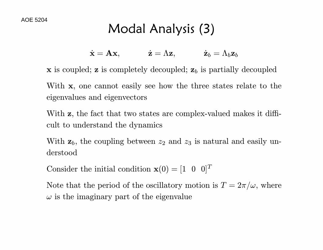
AOE 5204

Modal Analysis (4)

0 0.5 1 1.5 2 2.5 3 3.5−40

−20

0

20

40

60

80

100

t

x

x1

x2

x3

Initial state is x(0) = [1 0 0]T . Even though x2(0) = x3(0), all

three states diverge due to the coupling and the instability

AOE 5204

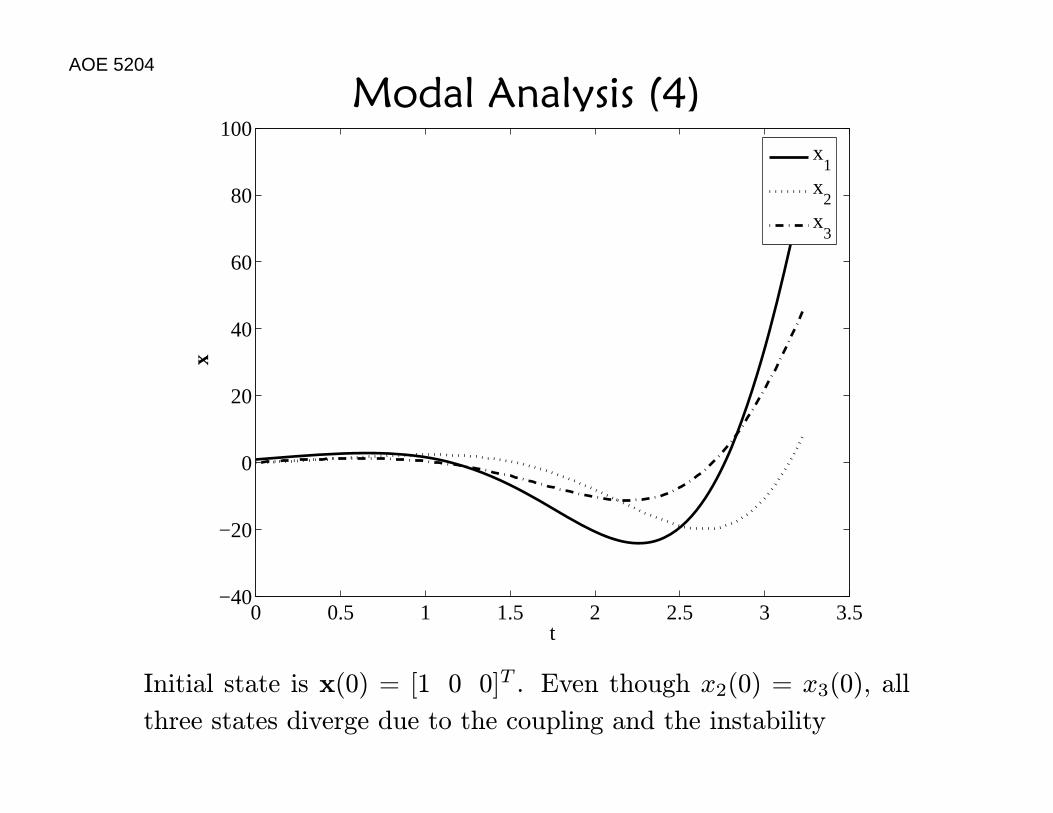
Modal Analysis (5)

0 0.5 1 1.5 2 2.5 3 3.5−100

−80

−60

−40

−20

0

20

40

t

z

z1

z2

z3

Initial state is x(0) = [1 0 0]T ⇒ z(0) = [−0.6897 − 1.4433 −1.1421]T . The state associated with the stable eigenvalue is not

unstable

AOE 5204

Modal Analysis (6)

0 0.5 1 1.5 2 2.5 3 3.5−0.7

−0.6

−0.5

−0.4

−0.3

−0.2

−0.1

0

0.1

t

z

z1

z2

z3

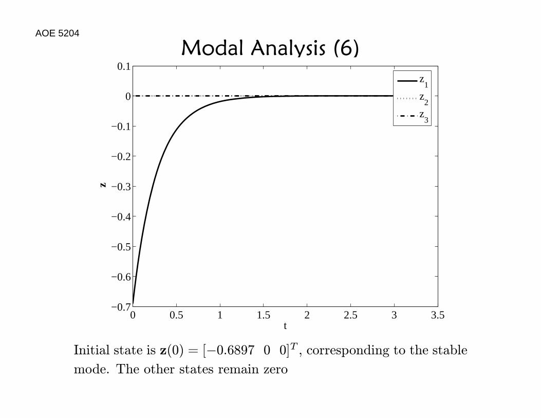
Initial state is z(0) = [−0.6897 0 0]T , corresponding to the stable

mode. The other states remain zero

AOE 5204

Modal Analysis (7)

0 0.5 1 1.5 2 2.5 3 3.5−100

−80

−60

−40

−20

0

20

40

t

z

z1

z2

z3

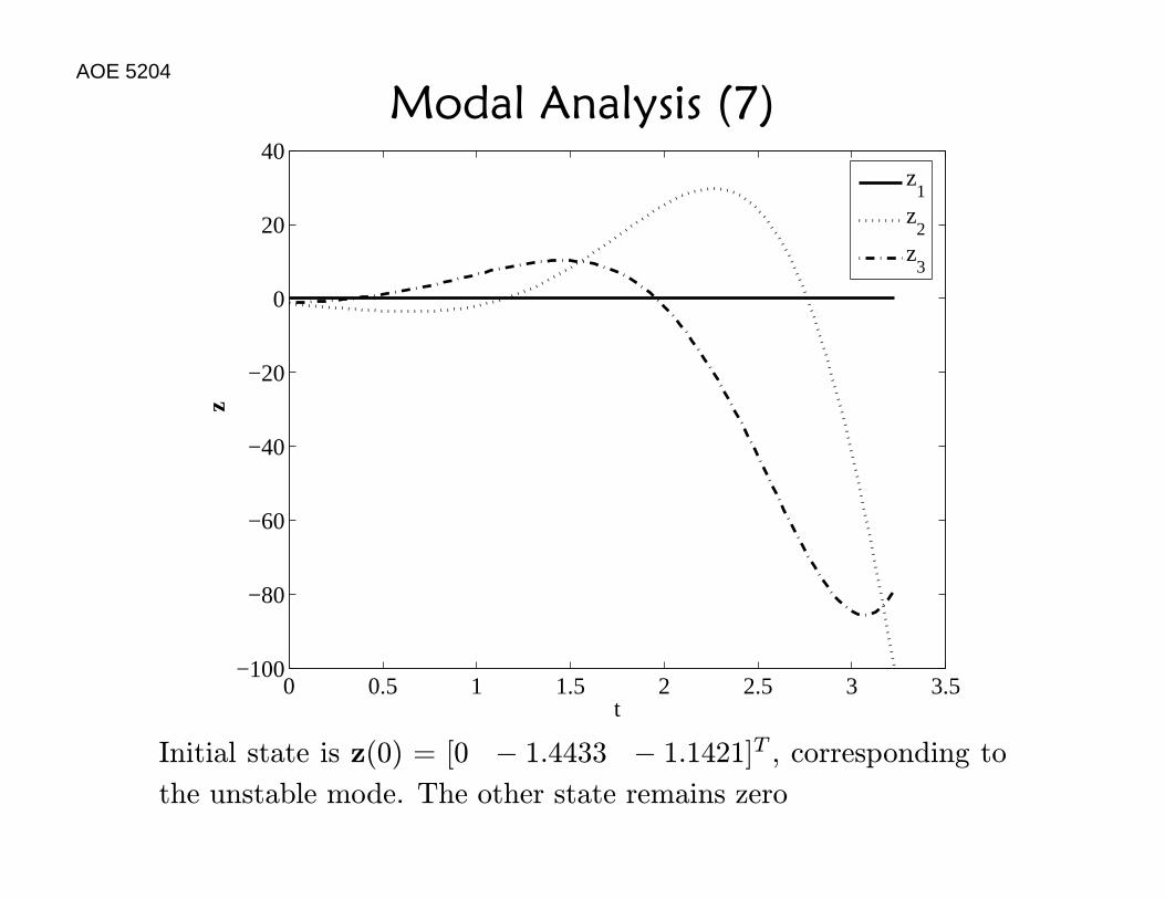
Initial state is z(0) = [0 − 1.4433 − 1.1421]T , corresponding tothe unstable mode. The other state remains zero

AOE 5204

Modal Analysis (8)

Modal analysis is based on block-diagonalizing x = Ax to obtain

zb = Λbzb

Whereas x is coupled, zb is partially decoupled

The real eigenvalues have one-dimensional real modes with expo-

nential (aka first-order) behavior

The complex conjugate eigenvalues have two-dimensional real

modes with exponential+oscillatory (aka second-order) behavior

By decomposing the motion into different modes, we can determine

the behavior of a dynamic system and focus attention on specific

modes of interest

Typically unstable, marginally stable, or barely stable modes are of

the most interest

AOE 5204

Back to the SolutionThe solution to the differential equation x = Ax is x(t) =

eAtx(0) = EeΛtE−1x(0), but what about

x = Ax+Bu ?

Consider the n = p = 1 case

x = ax+ u ⇒ x− ax = u

where a is constant and u is time-varying

One way to solve this first-order ODE is to turn the left-hand side

into a total derivative

Multiply by an unknown function y(t) and determine the form of

y(t) so that the left-hand side is d(xy)/dt

xy − axy = d

dt(xy) = xy + xy

AOE 5204

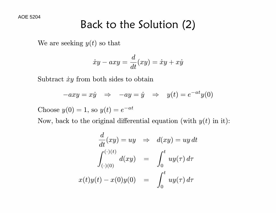
Back to the Solution (2)

We are seeking y(t) so that

xy − axy = d

dt(xy) = xy + xy

Subtract xy from both sides to obtain

−axy = xy ⇒ −ay = y ⇒ y(t) = e−aty(0)

Choose y(0) = 1, so y(t) = e−at

Now, back to the original differential equation (with y(t) in it):

d

dt(xy) = uy ⇒ d(xy) = uy dtZ (·)(t)

(·)(0)d(xy) =

Z t

0

uy(τ) dτ

x(t)y(t)− x(0)y(0) =

Z t

0

uy(τ) dτ

AOE 5204

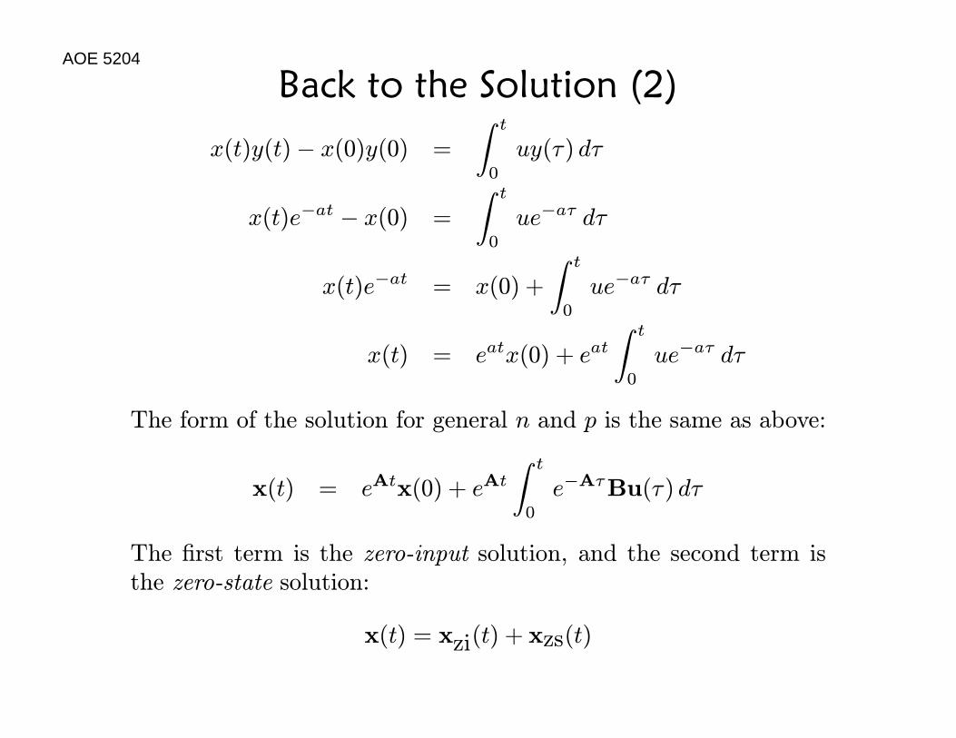
Back to the Solution (2)

x(t)y(t)− x(0)y(0) =

Z t

0

uy(τ) dτ

x(t)e−at − x(0) =

Z t

0

ue−aτ dτ

x(t)e−at = x(0) +

Z t

0

ue−aτ dτ

x(t) = eatx(0) + eatZ t

0

ue−aτ dτ

The form of the solution for general n and p is the same as above:

x(t) = eAtx(0) + eAtZ t

0

e−AτBu(τ) dτ

The first term is the zero-input solution, and the second term isthe zero-state solution:

x(t) = xzi(t) + xzs(t)

AOE 5204

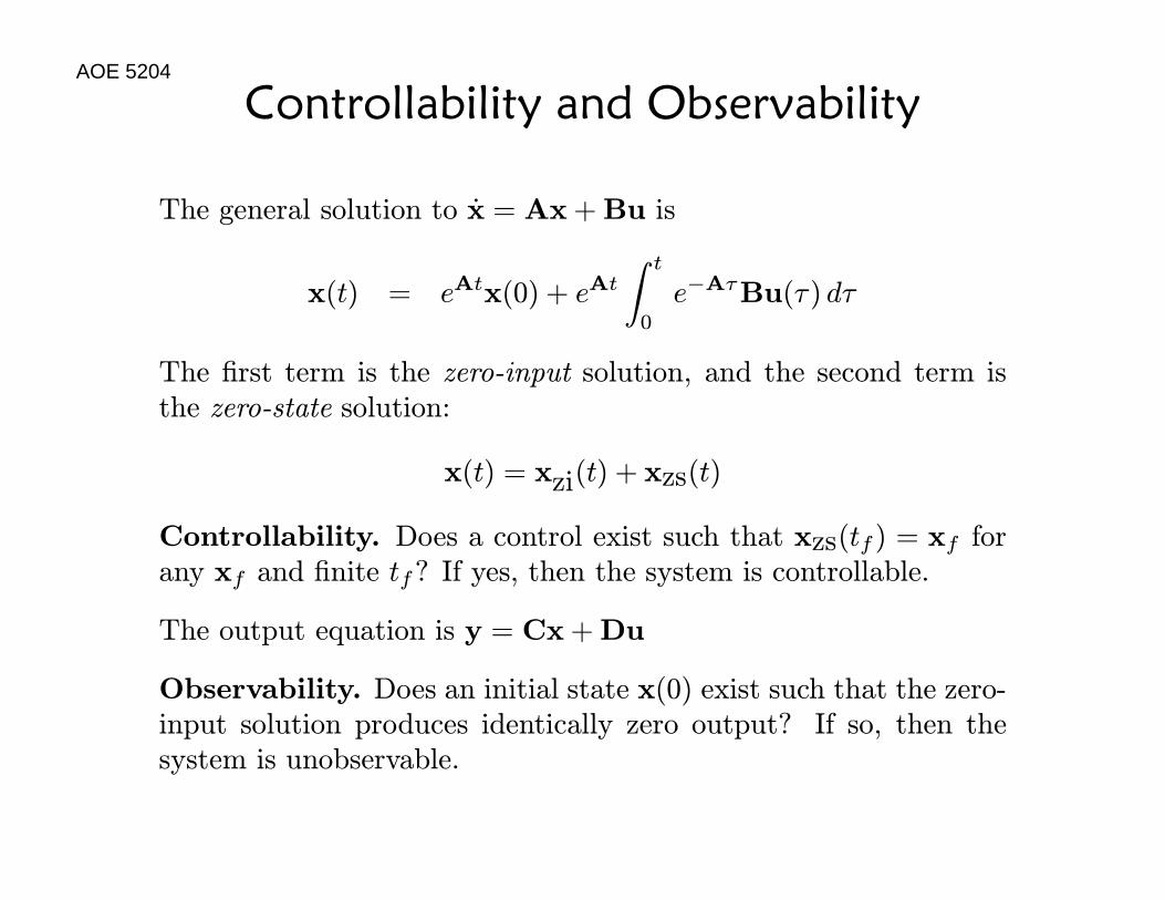
Controllability and Observability

The general solution to x = Ax+Bu is

x(t) = eAtx(0) + eAtZ t

0

e−AτBu(τ) dτ

The first term is the zero-input solution, and the second term isthe zero-state solution:

x(t) = xzi(t) + xzs(t)

Controllability. Does a control exist such that xzs(tf ) = xf forany xf and finite tf? If yes, then the system is controllable.

The output equation is y = Cx+Du

Observability. Does an initial state x(0) exist such that the zero-input solution produces identically zero output? If so, then thesystem is unobservable.

AOE 5204

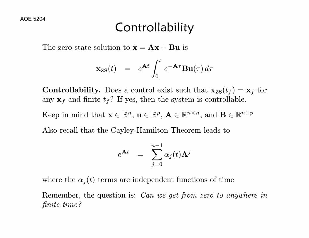
ControllabilityThe zero-state solution to x = Ax+Bu is

xzs(t) = eAtZ t

0

e−AτBu(τ) dτ

Controllability. Does a control exist such that xzs(tf ) = xf forany xf and finite tf? If yes, then the system is controllable.

Keep in mind that x ∈ Rn, u ∈ Rp, A ∈ Rn×n, and B ∈ Rn×p

Also recall that the Cayley-Hamilton Theorem leads to

eAt =n−1Xj=0

αj(t)Aj

where the αj(t) terms are independent functions of time

Remember, the question is: Can we get from zero to anywhere infinite time?

AOE 5204

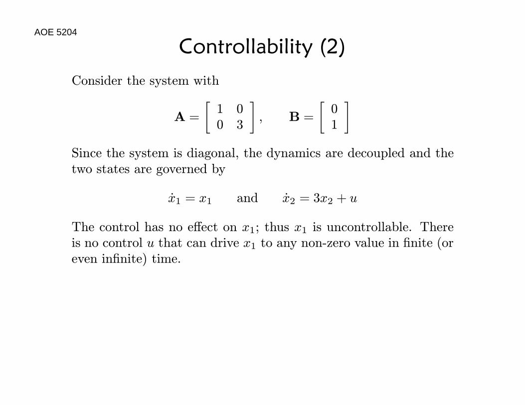
Controllability (2)Consider the system with

A =

∙1 00 3

¸, B =

∙01

¸Since the system is diagonal, the dynamics are decoupled and thetwo states are governed by

x1 = x1 and x2 = 3x2 + u

The control has no effect on x1; thus x1 is uncontrollable. Thereis no control u that can drive x1 to any non-zero value in finite (oreven infinite) time.

AOE 5204

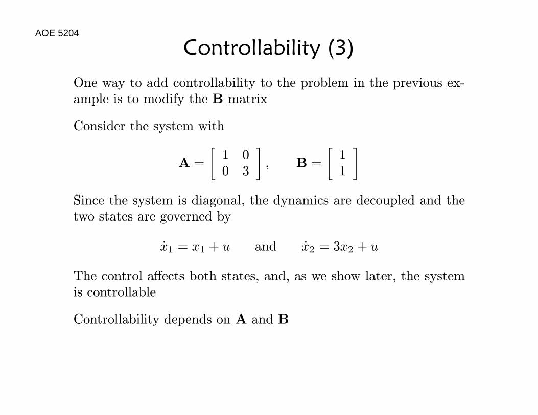
Controllability (3)One way to add controllability to the problem in the previous ex-ample is to modify the B matrix

Consider the system with

A =

∙1 00 3

¸, B =

∙11

¸Since the system is diagonal, the dynamics are decoupled and thetwo states are governed by

x1 = x1 + u and x2 = 3x2 + u

The control affects both states, and, as we show later, the systemis controllable

Controllability depends on A and B

AOE 5204

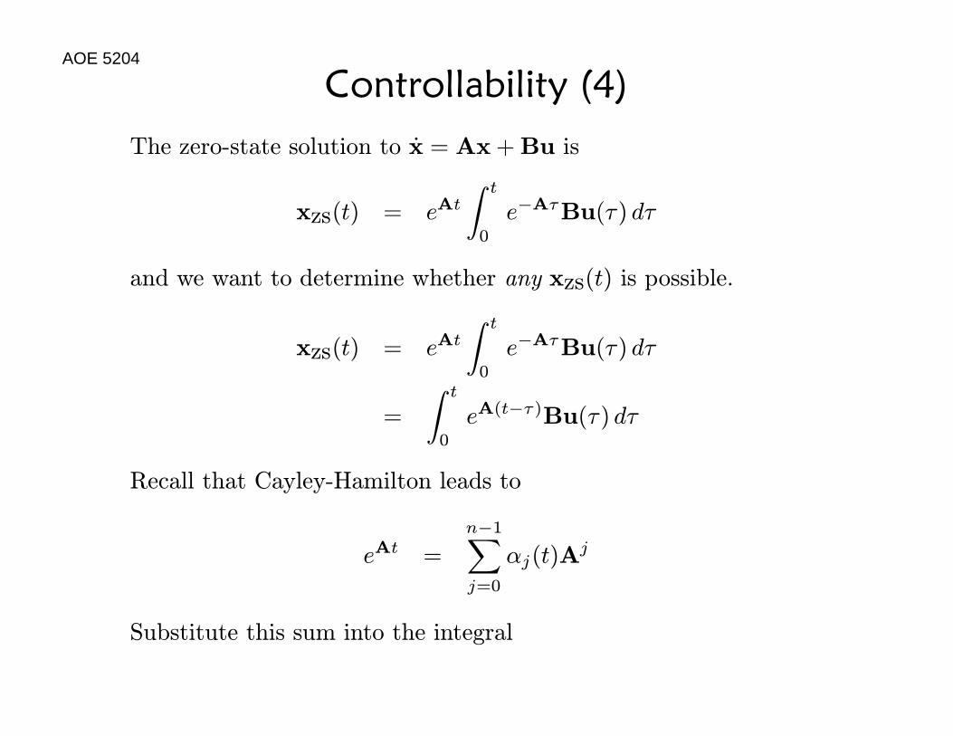
Controllability (4)The zero-state solution to x = Ax+Bu is

xzs(t) = eAtZ t

0

e−AτBu(τ) dτ

and we want to determine whether any xzs(t) is possible.

xzs(t) = eAtZ t

0

e−AτBu(τ) dτ

=

Z t

0

eA(t−τ)Bu(τ) dτ

Recall that Cayley-Hamilton leads to

eAt =n−1Xj=0

αj(t)Aj

Substitute this sum into the integral

AOE 5204

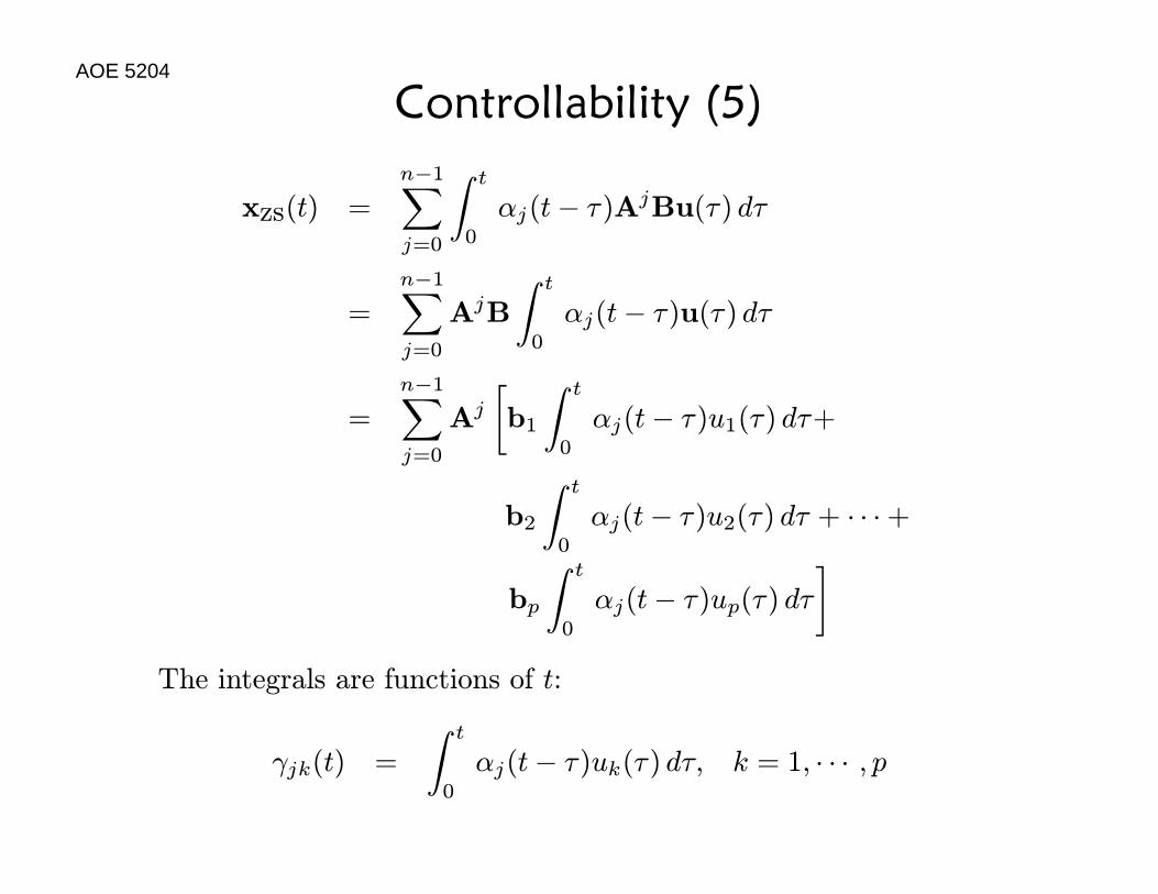
Controllability (5)

xzs(t) =n−1Xj=0

Z t

0

αj(t− τ)AjBu(τ) dτ

=n−1Xj=0

AjB

Z t

0

αj(t− τ)u(τ) dτ

=n−1Xj=0

Aj

∙b1

Z t

0

αj(t− τ)u1(τ) dτ+

b2

Z t

0

αj(t− τ)u2(τ) dτ + · · ·+

bp

Z t

0

αj(t− τ)up(τ) dτ¸

The integrals are functions of t:

γjk(t) =

Z t

0

αj(t− τ)uk(τ) dτ, k = 1, · · · , p

AOE 5204

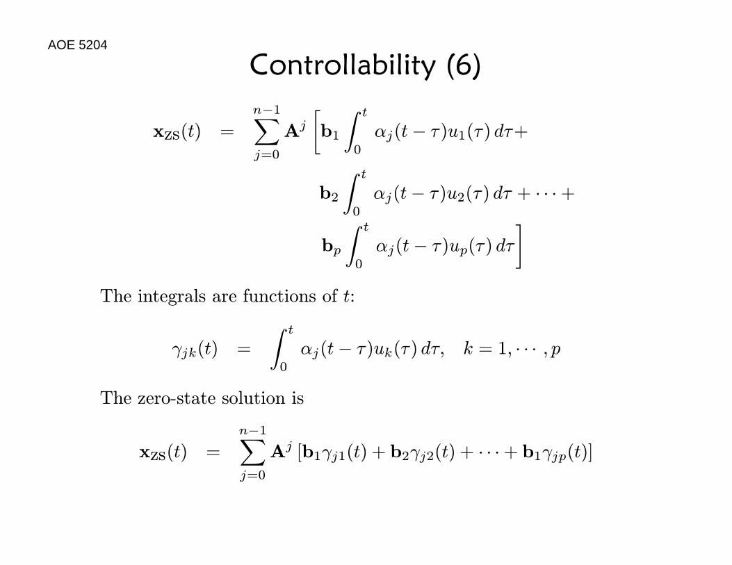
Controllability (6)

xzs(t) =n−1Xj=0

Aj

∙b1

Z t

0

αj(t− τ)u1(τ) dτ+

b2

Z t

0

αj(t− τ)u2(τ) dτ + · · ·+

bp

Z t

0

αj(t− τ)up(τ) dτ¸

The integrals are functions of t:

γjk(t) =

Z t

0

αj(t− τ)uk(τ) dτ, k = 1, · · · , p

The zero-state solution is

xzs(t) =n−1Xj=0

Aj [b1γj1(t) + b2γj2(t) + · · ·+ b1γjp(t)]

AOE 5204

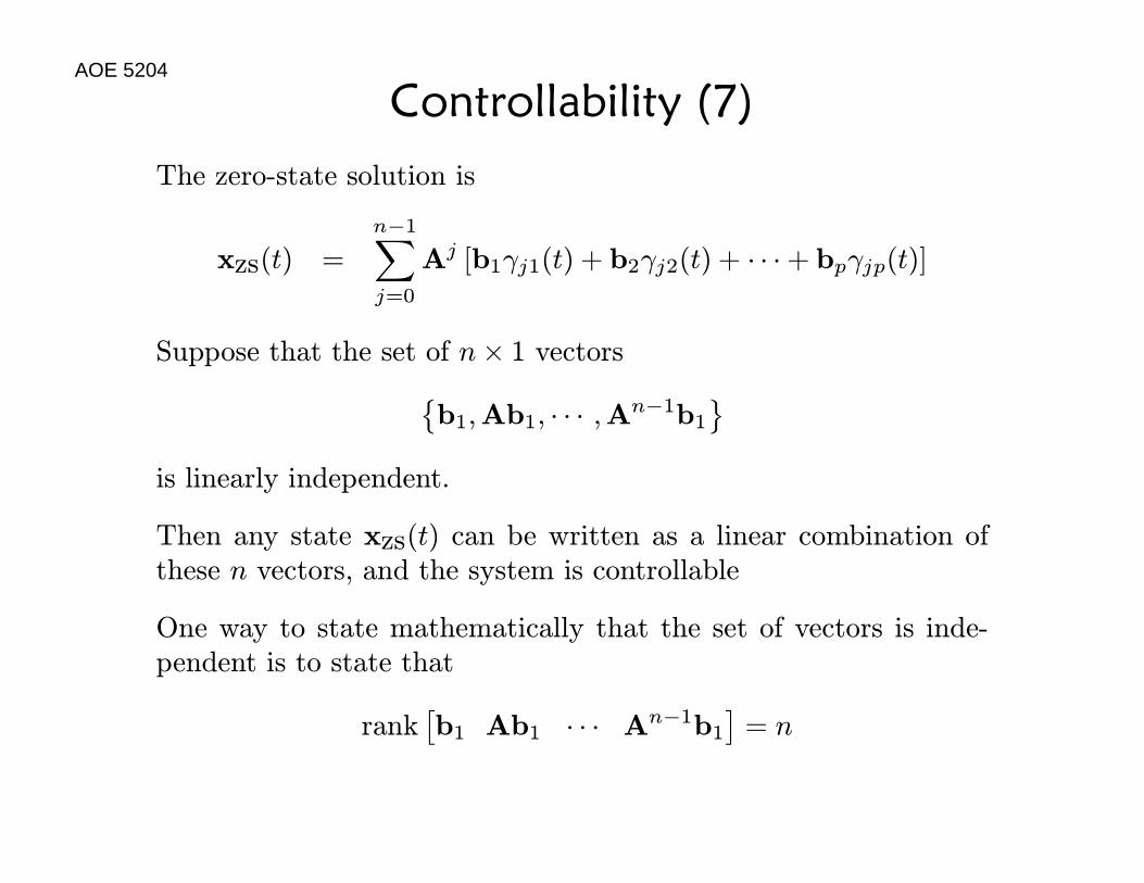
Controllability (7)The zero-state solution is

xzs(t) =n−1Xj=0

Aj [b1γj1(t) + b2γj2(t) + · · ·+ bpγjp(t)]

Suppose that the set of n× 1 vectors©b1,Ab1, · · · ,An−1b1

ªis linearly independent.

Then any state xzs(t) can be written as a linear combination ofthese n vectors, and the system is controllable

One way to state mathematically that the set of vectors is inde-pendent is to state that

rank£b1 Ab1 · · · An−1b1

¤= n

AOE 5204

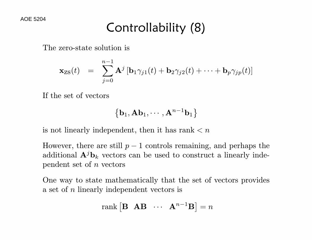
Controllability (8)The zero-state solution is

xzs(t) =n−1Xj=0

Aj [b1γj1(t) + b2γj2(t) + · · ·+ bpγjp(t)]

If the set of vectors ©b1,Ab1, · · · ,An−1b1

ªis not linearly independent, then it has rank < n

However, there are still p− 1 controls remaining, and perhaps theadditional Ajbk vectors can be used to construct a linearly inde-pendent set of n vectors

One way to state mathematically that the set of vectors providesa set of n linearly independent vectors is

rank£B AB · · · An−1B

¤= n

AOE 5204

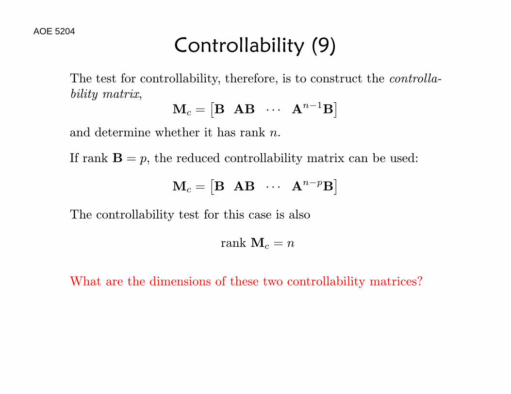
Controllability (9)The test for controllability, therefore, is to construct the controlla-bility matrix,

Mc =£B AB · · · An−1B

¤and determine whether it has rank n.

If rank B = p, the reduced controllability matrix can be used:

Mc =£B AB · · · An−pB

¤The controllability test for this case is also

rank Mc = n

What are the dimensions of these two controllability matrices?

AOE 5204

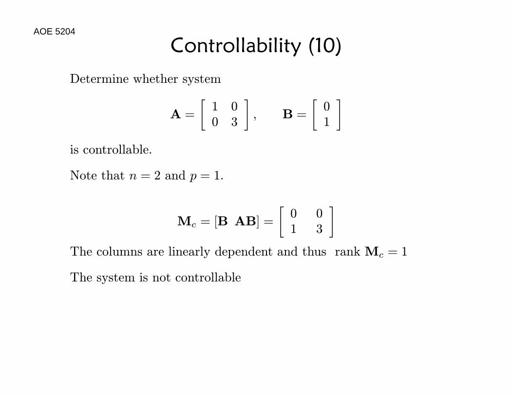
Controllability (10)Determine whether system

A =

∙1 00 3

¸, B =

∙01

¸is controllable.

Note that n = 2 and p = 1.

Mc = [B AB] =

∙01

03

¸The columns are linearly dependent and thus rank Mc = 1

The system is not controllable

AOE 5204

Controllability (11)Determine whether system

A =

∙1 00 3

¸, B =

∙11

¸is controllable.

Note that n = 2 and p = 1.

Mc = [B AB] =

∙11

13

¸The columns are linearly independent and thus rank Mc = 2

The system is controllable

AOE 5204

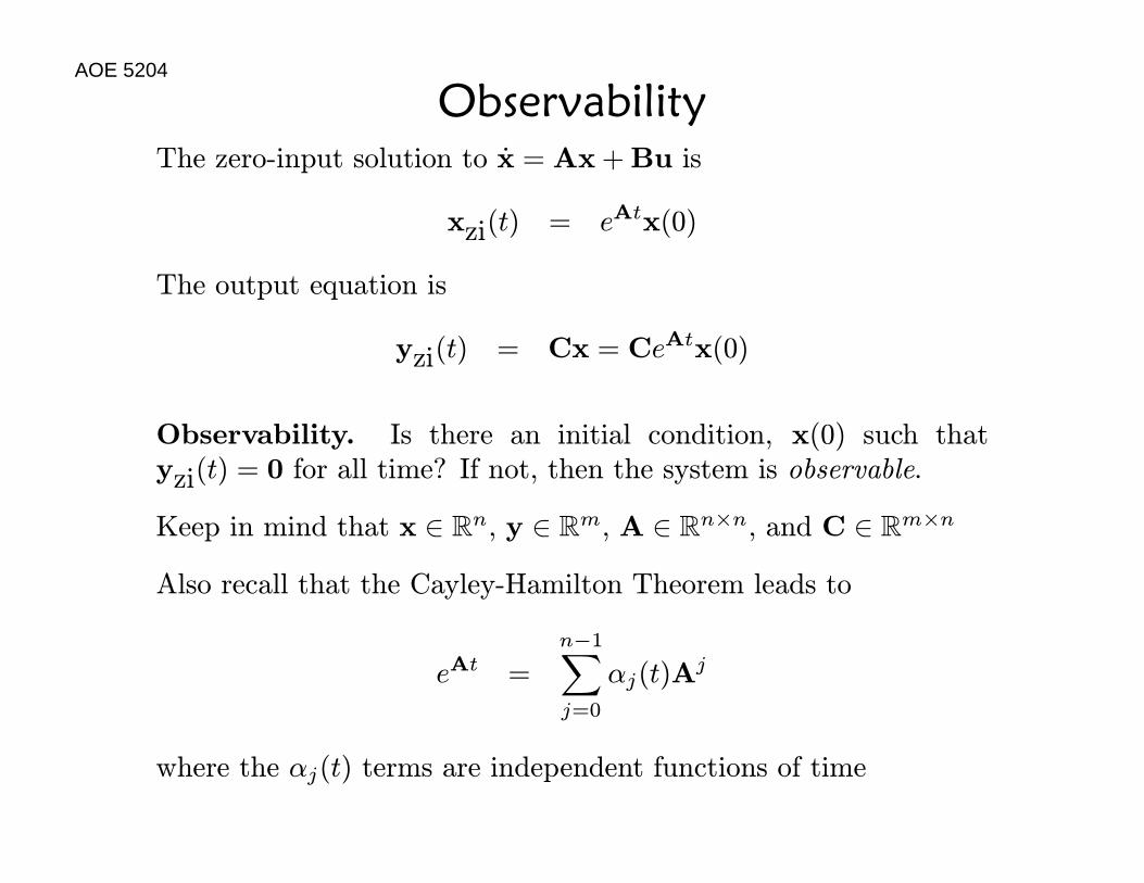
ObservabilityThe zero-input solution to x = Ax+Bu is

xzi(t) = eAtx(0)

The output equation is

yzi(t) = Cx = CeAtx(0)

Observability. Is there an initial condition, x(0) such thatyzi(t) = 0 for all time? If not, then the system is observable.

Keep in mind that x ∈ Rn, y ∈ Rm, A ∈ Rn×n, and C ∈ Rm×n

Also recall that the Cayley-Hamilton Theorem leads to

eAt =n−1Xj=0

αj(t)Aj

where the αj(t) terms are independent functions of time