Embed Size (px)
Citation preview
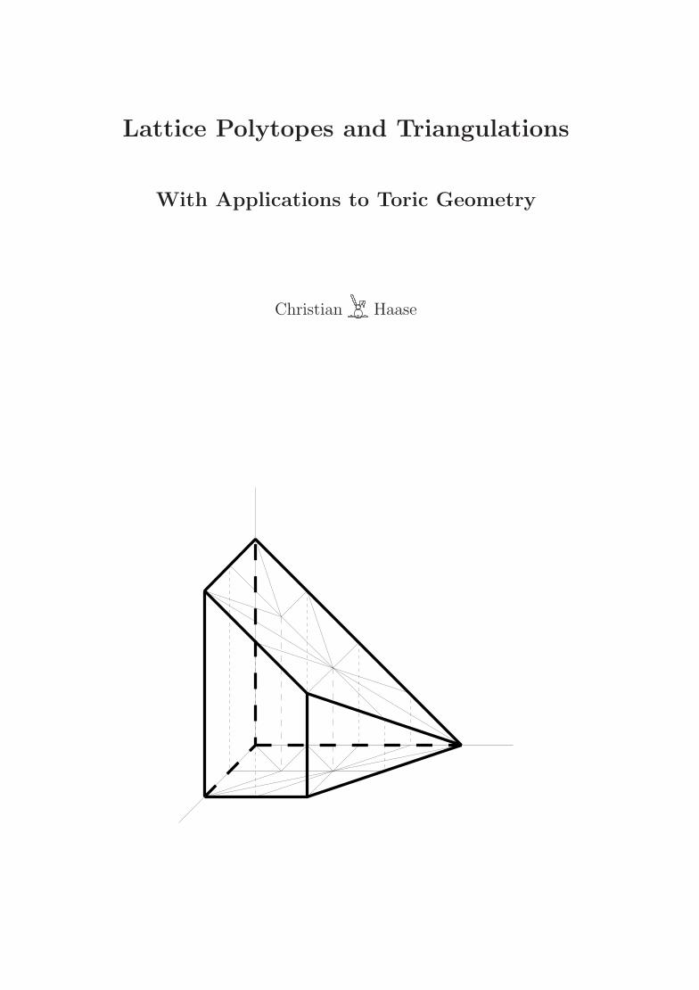
Lattice Polytopes and Triangulations
With Applications to Toric Geometry
Christian Haase

2
Lattice Polytopes and Triangulations
With Applications to Toric Geometry
vorgelegt vonDiplom–Mathematiker
Christian Alexander Haase
Vom Fachbereich Mathematikder Technischen Universitat Berlin
zur Erlangung des akademischen Grades
Doktor der NaturwissenschaftenDr. rer. nat.
genehmigte Dissertation.
Promotionsausschuß:
Vorsitzender: Prof. Dr. Rolf Dieter GrigorieffBerichter: Prof. Dr. Gunter M. ZieglerBerichter: PD. Dr. Klaus Altmann
Tag der wissenschaftlichen Aussprache: 17. Januar 2000
Berlin 2000
D 83

4
5
Thanks!In 1996, I was about to finish being an undergraduate. What should I become asan adult? I could do real–world work and get rich, or I could be a mathematicianand have fun — only where, what, how? At the time, there were no universityposts for graduates, at least not in Berlin. In order to come to an end, I plannednot to take part in any courses anymore, but to “dedicate my full working power”1
to my Diplomarbeit2 in algebraic topology. Nice plan, but as I do not like bigdecisions, I pushed my deadline further and further. Part of this strategy, I couldnot avoid the lecture entitled Discrete structures and their topology, given bya certain professor Gunter Ziegler. This was my first contact with discretemathematics. In a discussion about the perspectives of graduates, this GunterZiegler mentioned that a graduate school could be an alternative to the usualuniversity positions. Then he presented a number of challenging mathematicalproblems to me that could be the subject of a dissertation.
So there was my decision, and there was my deadline: Bettina Felsner,the secretary of the graduate school Algorithmische diskrete Mathematik3,wanted a copy of my Diplomarbeit by January 1997. Suddenly, I really had tofinish quickly. Marion and Volkmar Scholz supplied me with the necessarycopying power and I was admitted. I started my discrete career in a very stim-ulating environment: the Berlin discrete community assembled in the graduateschool and at the TU–Berlin, and remainders of the topological family around myformer advisor professor Elmar Vogt helped me in many tea time discussionsand built up this great atmosphere. One cannot overestimate the contribution ofice cream devouring Bettina Felsner in this context.
Gunter Ziegler taught me how to research, how to give talks and much more.His door was always open for me, even when he had a huge pile of work on his desk.He introduced me to Dimitrios Dais, a very enthusiastic algebraic geometer,who reported lots of known and unknown algebraic geometry to me, preventedme from writing algebraic non–sense, and who co–authored Chapters III and IV.Once written down, this thesis had to pass my referees Carsten Lange, GunterPaul Leiterer, Mark de Longueville, Frank Lutz, Eva–Nuria Muller andCarsten Schultz.
So much about my academic support. Personally, I was supported by mytwo women: My mother Heide Haase did everything one can imagine that amother can do — and a little bit more. In particular, I want to mention her helpconcerning my friends from Y–town4. My girlfriend Kerstin Theurer got medown to earth from time to time. I completely rely on the backing and love shegives to me.
Thank you all, .1From: Richtlinien fur Stipendiaten [GK, p. 2]2Diploma thesis.3Algorithmic discrete mathematics, DFG grant GRK 219/3.4German Bundeswehr.

6
Contents
Chapter I. Introduction 91. What, why, who? 92. Notions from discrete and convex geometry 123. Notions from algebraic and toric geometry 184. From the dictionary 20
Chapter II. Lattice width of empty simplices 231. Introduction 232. Adding one dimension 263. Computer search in dimension 4 31
Chapter III. Crepant resolutions of toric l.c.i.–singularities 391. Introduction 392. Proof of the Main Theorem 423. Applications 45
Chapter IV. Stringy Hodge numbers of hypersurfaces in toric varieties 511. Introduction 512. Symmetric Fano polytopes 583. Pyramids over Fano polytopes 67
Bibliography 79
7

8 CONTENTS
CHAPTER I
Introduction
1. What, why, who?
This is a commercial. I want you to become friends with lattice polytopes.A lattice polytope is the convex hull of finitely many points from a given grid orlattice (usually Zd). The interaction between the combinatorial, geometric andalgebraic information encoded makes them rewarding objects of study: Manyalgebraic or combinatorial results have a proof that uses lattice polytopes, andmethods from the whole mathematical landscape are used to deal with latticepolytope problems.
Triangulations provide an important device in our tool box. In many circum-stances it is useful to split a given lattice polytope into smaller pieces of simplerstructure. The easiest (but by far not easy) species to handle are the simplices:the convex hull of affinely independent points. Usually there are several ways totriangulate a lattice polytope, i.e., to subdivide it into simplices. So it is naturalto ask for ‘good’ triangulations for the specific problem. An example of a crite-rion for a ‘good’ triangulation is unimodularity: a (full dimensional) simplex isunimodular if, by integral affine combinations of its vertices one can reach thewhole lattice. The problem about unimodular triangulations is that they do notalways (only rarely ?) exist.
One of the many applications of lattice polytopes lies in the field of toricgeometry. The discrete geometric object “lattice polytope” has an algebro geo-metric brother, a toric variety. It is amazing how discrete properties find theiralgebraic counterparts, how seemingly combinatorial results have algebraic proofs(and vice versa).
There are many other fields where lattice polytopes show up. Whether youcome from discrete optimization, algebraic geometry, commutative algebra orgeometry of numbers you have already seen them in action. On the other hand,methods from combinatorics, algebra and analysis are assembled in order to tacklelattice polytope problems. But let us get concrete.
For example, in discrete optimization and in geometry of numbers, latticepolytopes arise as the convex hull of the lattice points in a given convex body B.Fundamental problems in the area are the feasibility problem “B ∩ Zd = ∅?”,and, more general, the counting problem “card(B ∩ Zd) = ?”. The answer in
9
10 I. INTRODUCTION
dimension 2, Pick’s famous formula
Vol(P ) = card(P ∩ Z2) − card(∂P ∩ Z2)
2− 1 , P ⊂ R2 a lattice polygon,
follows from the fact that polygons always admit unimodular triangulations. Thisdoes no longer hold in dimensions ≥ 3. Even worse, both above problems proveto be NP-hard when the dimension varies. Though, if the dimension is notconsidered as part of the input, Lenstra [Len83] used the concept of lattice widthand an algorithmic version of the Flatness Theorem (cf. Chapter II) to provide apolynomial time algorithm for the feasibility problem. (The best known flatness–bound has an analytical proof [BLPS98].) Barvinok [Bar94] applied ‘weighted’unimodular triangulations of cones to count lattice points in fixed dimension inpolynomial time.
A unimodular triangulation, if it exists, tells you a lot about the polytope.E.g., the numbers of the simplices of the various dimensions completely deter-mines (and is determined by) the Ehrhart polynomial, which counts lattice pointsin dilations of the polytope.
card(k · P ∩ Zd) = Ehr(P, k) =d∑
i=0
ai(P )ki for k ≥ 0.
Unfortunately, the typical lattice polytope does not admit such nice triangula-tions. One can try to weaken the triangulation property by several dissection orcovering properties [BGT97, FZ99, Seb90]. But even a unimodular cover doesnot always exist. The situation changes if the polytope of concern is enlarged.In [KKMSD73], Knudsen and Mumford proved that each polytope can be mul-tiplied by a factor to obtain a polytope with a unimodular triangulation. Bruns,Gubeladze and Trung [BGT97] show that a unimodular cover exists for all largeenough factors.
In commutative algebra one associates a graded affine semigroup with a lat-tice polytope. The above covering/triangulation properties translate to algebraicproperties of the semigroup ring and its Grobner bases [BG99, BGH+99, BGT97,Stu96].
Interestingly, the meanest examples with respect to these properties are the(non–unimodular) empty lattice simplices, simplices that do not contain any lat-tice points other than the vertices. They correspond to so called terminal singular-ities in toric geometry. White’s Theorem which bounds the lattice width of emptylattice tetrahedra by 1 is the key ingredient in the classification of 3–dimensionalterminal Abelian quotient singularities, i.e., of empty lattice tetrahedra [MS84].
This thesis takes you to three sites in the lattice polytope landscape with afocus on the algebraic geometry borderline. We visit the family of empty latticesimplices (Chapter II), which are flat by Khinchine’s Flatness Theorem. But
1. WHAT, WHY, WHO? 11
they are not as flat as one could expect. We present examples in dimension4, and some constructions how to obtain thick d–simplices from thick (d − 1)–dimensional ones. These results together disprove Barany’s pancake conjecture:thick empty simplices may have huge volume. The results of this chapter haveappeared as [HZ00]. This is joint work with Gunter Ziegler.
At our next stop (Chapter III), we look at those lattice polytopes whose toricbrothers are local complete intersections (l.c.i.). We will see that they are nottypical, in the sense that they do admit unimodular triangulations. So theirbrothers have nice resolutions. This supports the conjecture that any l.c.i. (notnecessarily toric) admits such resolutions. This joint work with Dimitrios Daisand Gunter Ziegler will appear as [DHZ00] (cf. also [DHZ98a]).
The last two locations (Chapter IV) present incidences of the above countingproblem. This time there is no conjecture behind — well, there is one, far behind.Related to the mirror symmetry conjecture from theoretical physics, Batyrev andDais [BD96] constructed certain invariants of varieties, the string theoretic Hodgenumbers. We open a small zoo of examples for which these invariants can actuallybe computed. Therefore we have to evaluate Ehrhart polynomials and some otherdata. This is joint work with Dimitrios Dais [DHa].
This will finish our little journey. It will hopefully convince you of the beautyof the whole area and motivate you to explore the many unknown spots. Butbefore we can really start, we have to work ourselves through a jungle of defini-tions and notation (the next three sections of this chapter.) I have tried to makeit short and painless. Have a nice trip. . .
12 I. INTRODUCTION
2. Notions from discrete and convex geometry
2.1. General notation. The convex hull and the affine hull of a set S ⊂ Rd
are denoted by conv(S) and aff(S), respectively. The dimension dim(S) of S isthe dimension of aff(S); the relative interior relint(S) is the interior with respectto aff(S). A polyhedron Q is a finite intersection of closed halfspaces in Rd. Thesubset F ⊆ Q that minimizes some linear functional on Q is a face of Q; wewrite F ¹ Q, and F ≺ Q if we want to exclude equality (F is a proper face).Zero–dimensional faces are called vertices, 1–dimensional bounded faces are edges,unbounded ones rays and (dim Q − 1)–dimensional faces are facets. The facesof a polyhedron form a partially ordered set (poset) with respect to inclusion.Denote by fk(Q) the number of k–dimensional faces of Q.
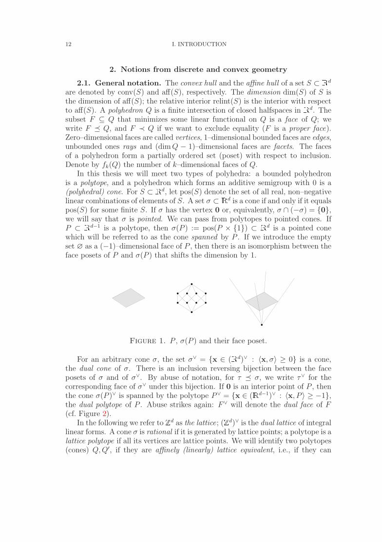
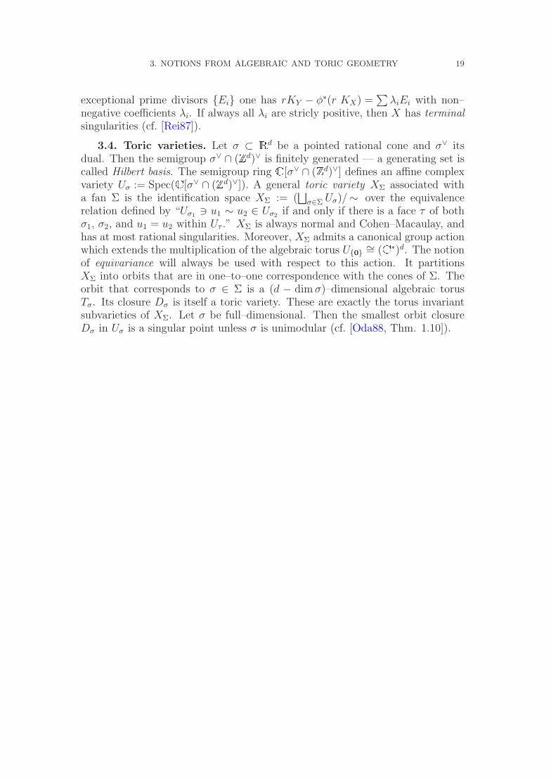
In this thesis we will meet two types of polyhedra: a bounded polyhedronis a polytope, and a polyhedron which forms an additive semigroup with 0 is a(polyhedral) cone. For S ⊂ Rd, let pos(S) denote the set of all real, non–negativelinear combinations of elements of S. A set σ ⊂ Rd is a cone if and only if it equalspos(S) for some finite S. If σ has the vertex 0 or, equivalently, σ ∩ (−σ) = 0,we will say that σ is pointed. We can pass from polytopes to pointed cones. IfP ⊂ Rd−1 is a polytope, then σ(P ) := pos(P × 1) ⊂ Rd is a pointed conewhich will be referred to as the cone spanned by P . If we introduce the emptyset ∅ as a (−1)–dimensional face of P , then there is an isomorphism between theface posets of P and σ(P ) that shifts the dimension by 1.
Figure 1. P , σ(P ) and their face poset.
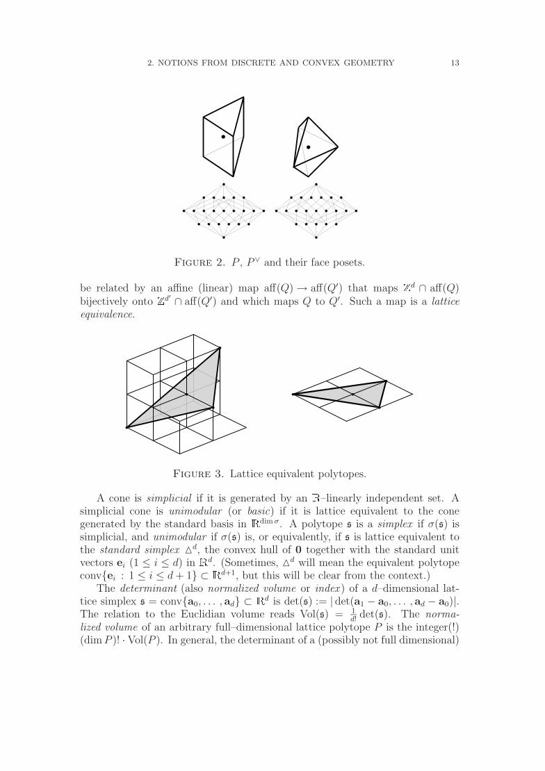
For an arbitrary cone σ, the set σ∨ = x ∈ (Rd)∨ : 〈x, σ〉 ≥ 0 is a cone,the dual cone of σ. There is an inclusion reversing bijection between the faceposets of σ and of σ∨. By abuse of notation, for τ ¹ σ, we write τ∨ for thecorresponding face of σ∨ under this bijection. If 0 is an interior point of P , thenthe cone σ(P )∨ is spanned by the polytope P∨ = x ∈ (Rd−1)∨ : 〈x, P 〉 ≥ −1,the dual polytope of P . Abuse strikes again: F∨ will denote the dual face of F(cf. Figure 2).
In the following we refer to Zd as the lattice; (Zd)∨ is the dual lattice of integrallinear forms. A cone σ is rational if it is generated by lattice points; a polytope is alattice polytope if all its vertices are lattice points. We will identify two polytopes(cones) Q,Q′, if they are affinely (linearly) lattice equivalent, i.e., if they can
2. NOTIONS FROM DISCRETE AND CONVEX GEOMETRY 13
Figure 2. P , P∨ and their face posets.
be related by an affine (linear) map aff(Q) → aff(Q′) that maps Zd ∩ aff(Q)bijectively onto Zd′ ∩ aff(Q′) and which maps Q to Q′. Such a map is a latticeequivalence.
Figure 3. Lattice equivalent polytopes.
A cone is simplicial if it is generated by an R–linearly independent set. Asimplicial cone is unimodular (or basic) if it is lattice equivalent to the conegenerated by the standard basis in Rdim σ. A polytope s is a simplex if σ(s) issimplicial, and unimodular if σ(s) is, or equivalently, if s is lattice equivalent tothe standard simplex Md, the convex hull of 0 together with the standard unitvectors ei (1 ≤ i ≤ d) in Rd. (Sometimes, Md will mean the equivalent polytopeconvei : 1 ≤ i ≤ d + 1 ⊂ Rd+1, but this will be clear from the context.)
The determinant (also normalized volume or index ) of a d–dimensional lat-tice simplex s = conva0, . . . , ad ⊂ Rd is det(s) := | det(a1 − a0, . . . , ad − a0)|.The relation to the Euclidian volume reads Vol(s) = 1
d!det(s). The norma-
lized volume of an arbitrary full–dimensional lattice polytope P is the integer(!)(dim P )! · Vol(P ). In general, the determinant of a (possibly not full dimensional)
14 I. INTRODUCTION
simplex s = conv0, a1, . . . , ak ⊂ Rd is the gcd of all (k × k)–minors of the ma-trix A with columns ai: This gcd is not changed if one applies an integral lineartransformation which differs from the identity only by one off–diagonal entry.These matrices, together with the permutations, generate the group of linear lat-tice equivalences. These can be used to transform A into the form
(A′0
), where A′
is a (k × k)–matrix with det(s) = det(A′).A lattice polytope is empty (also called elementary or lattice point free) if
its vertices are the only lattice points it contains. Every unimodular simplexis empty, but the converse is not true in dimensions d ≥ 3 (cf. the proof ofProposition II.2.1). A lattice polytope, which contains the unique interior latticepoint 0 and whose dual has again integral vertices, is called reflexive.
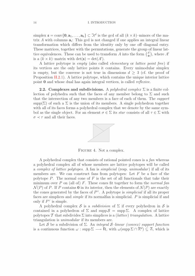
2.2. Complexes and subdivisions. A polyhedral complex Σ is a finite col-lection of polyhedra such that the faces of any member belong to Σ and suchthat the intersection of any two members is a face of each of them. The supportsupp(Σ) of such a Σ is the union of its members. A single polyhedron togetherwith all of its faces forms a polyhedral complex that we denote by the same sym-bol as the single object. For an element σ ∈ Σ its star consists of all τ ∈ Σ withσ ≺ τ and all their faces.
Figure 4. Not a complex.
A polyhedral complex that consists of rational pointed cones is a fan whereasa polyhedral complex all of whose members are lattice polytopes will be calleda complex of lattice polytopes. A fan is simplicial (resp. unimodular) if all of itsmembers are. We can construct fans from polytopes: Let F be a face of thepolytope P . The normal cone of F is the set of all functionals that take theirminimum over P on (all of) F . These cones fit together to form the normal fanN (P ) of P . If P contains 0 in its interior, then the elements of N (P ) are exactlythe cones generated by the faces of P∨. A polytope is simplicial if all its properfaces are simplices and simple if its normalfan is simplicial. P is simplicial if andonly if P∨ is simple.
A polyhedral complex S is a subdivision of Σ if every polyhedron in S iscontained in a polyhedron of Σ and suppS = supp Σ. A complex of latticepolytopes T that subdivides Σ into simplices is a (lattice) triangulation. A latticetriangulation is unimodular if its members are.
Let S be a subdivision of Σ. An integral S–linear (convex) support functionis a continuous function ω : supp Σ −→ R, with ω(supp Σ ∩ Zd) ⊆ Z, which is
2. NOTIONS FROM DISCRETE AND CONVEX GEOMETRY 15
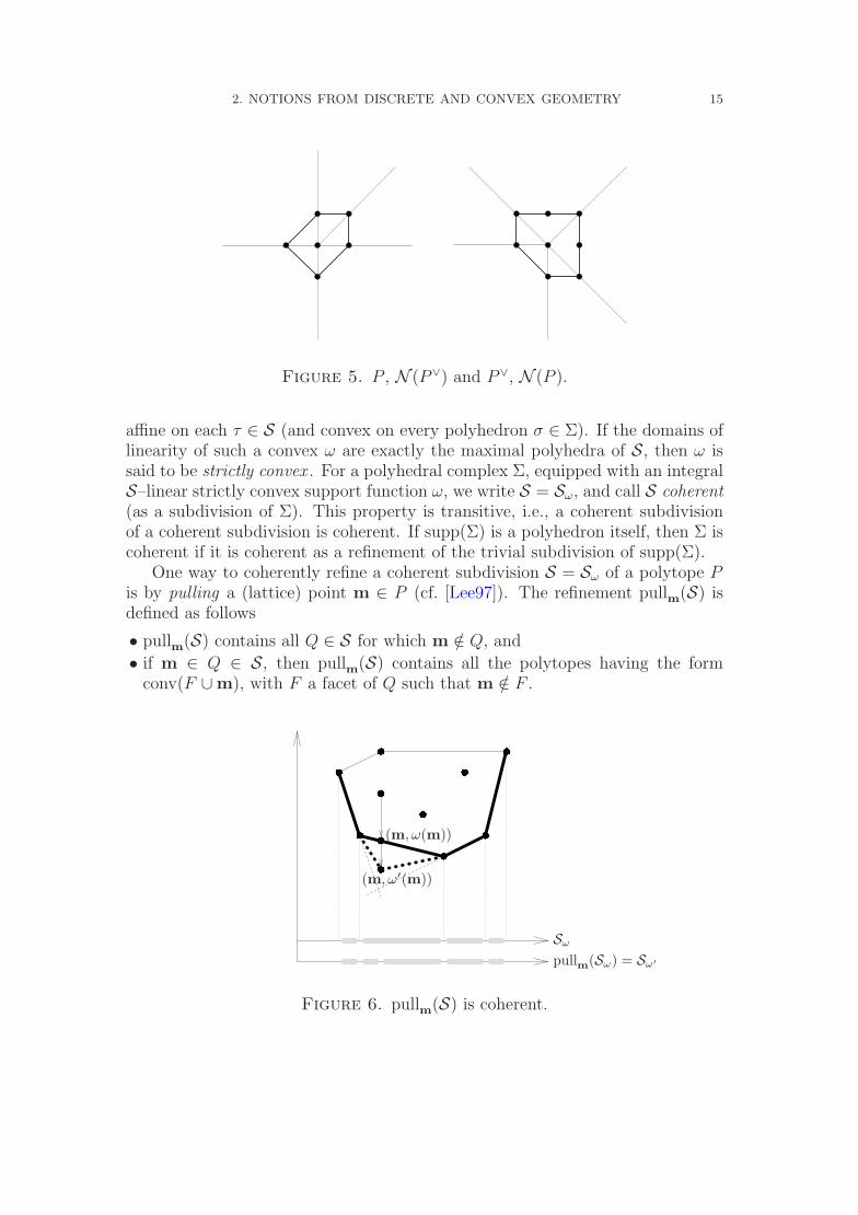
Figure 5. P , N (P∨) and P∨, N (P ).
affine on each τ ∈ S (and convex on every polyhedron σ ∈ Σ). If the domains oflinearity of such a convex ω are exactly the maximal polyhedra of S, then ω issaid to be strictly convex . For a polyhedral complex Σ, equipped with an integralS–linear strictly convex support function ω, we write S = Sω, and call S coherent(as a subdivision of Σ). This property is transitive, i.e., a coherent subdivisionof a coherent subdivision is coherent. If supp(Σ) is a polyhedron itself, then Σ iscoherent if it is coherent as a refinement of the trivial subdivision of supp(Σ).
One way to coherently refine a coherent subdivision S = Sω of a polytope Pis by pulling a (lattice) point m ∈ P (cf. [Lee97]). The refinement pullm(S) isdefined as follows
• pullm(S) contains all Q ∈ S for which m /∈ Q, and
• if m ∈ Q ∈ S, then pullm(S) contains all the polytopes having the formconv(F ∪ m), with F a facet of Q such that m /∈ F .
Sω
pullm(Sω) = Sω′
(m, ω(m))
(m, ω′(m))
Figure 6. pullm(S) is coherent.
16 I. INTRODUCTION
By pulling successively all the lattice points within a given lattice polytopeP one obtains a triangulation into empty simplices. If S = Sω is coherent, thenpullm(S) is obtained by “pulling m from below”. This means that, definingω′(m) = ω(m) − ε for ε small enough, and ω′ = ω on the remaining latticepoints, and extending ω′ by the maximal convex function ω′′ whose values at thelattice points are not greater than the given ones, we get pullm(S) = Sω′′ . Hence,if S is coherent, then so is pullm(S).
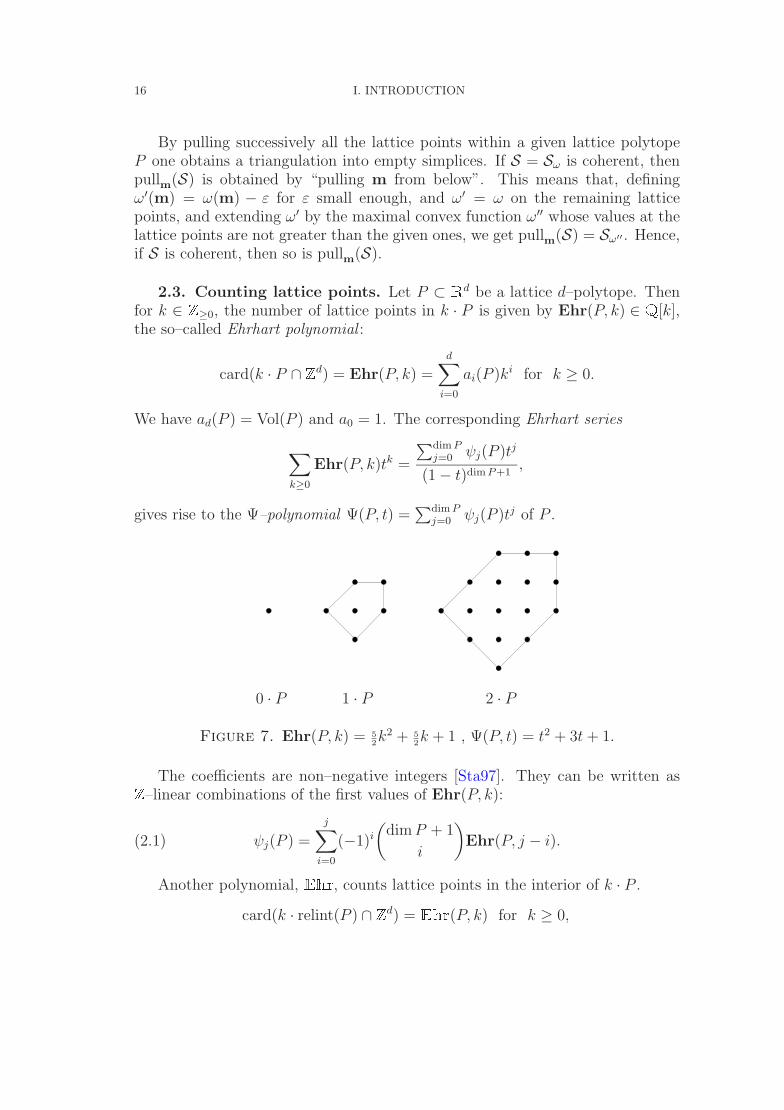
2.3. Counting lattice points. Let P ⊂ Rd be a lattice d–polytope. Thenfor k ∈ Z≥0, the number of lattice points in k · P is given by Ehr(P, k) ∈ Q[k],the so–called Ehrhart polynomial :
card(k · P ∩ Zd) = Ehr(P, k) =d∑
i=0
ai(P )ki for k ≥ 0.
We have ad(P ) = Vol(P ) and a0 = 1. The corresponding Ehrhart series
∑k≥0
Ehr(P, k)tk =
∑dim Pj=0 ψj(P )tj
(1 − t)dim P+1,
gives rise to the Ψ–polynomial Ψ(P, t) =∑dim P
j=0 ψj(P )tj of P .
1 · P 2 · P0 · P
Figure 7. Ehr(P, k) = 52k2 + 5
2k + 1 , Ψ(P, t) = t2 + 3t + 1.
The coefficients are non–negative integers [Sta97]. They can be written asZ–linear combinations of the first values of Ehr(P, k):
ψj(P ) =
j∑i=0
(−1)i
(dim P + 1
i
)Ehr(P, j − i).(2.1)
Another polynomial, Ehr, counts lattice points in the interior of k · P .
card(k · relint(P ) ∩ Zd) = Ehr(P, k) for k ≥ 0,
2. NOTIONS FROM DISCRETE AND CONVEX GEOMETRY 17
with interior Ehrhart series∑k≥0
Ehr(P, k)tk =
∑dim P+1j=1 ϕj(P )tj
(1 − t)dim P+1,
giving rise to the Φ–polynomial. The following well known reciprocity law holds[Ehr77, Sta97].
Ehr(P, k) = (−1)dim PEhr(P,−k).(2.2)
This implies:
2.1. Proposition. For any lattice polytope P , Φ(P, t) = tdim P+1Ψ(P, t−1) or,in other “words”, φj(P ) = ψdim P−j+1(P ).
Proof. The statement is true for the standard simplex. This follows fromEhr(Md, k) =
(k+d
d
), Ehr(Md, k) =
(k−1
d
)and Ψ(Md, t) = 1, Φ(Md, t) = td+1. The
Ehrhart polynomials of these simplices form a basis of Q[k]: any (Ehrhart) poly-
nomial can be written (uniquely) in the form∑dim P
i=0 λi
(k+i
i
). Then, by (2.2), the
interior Ehrhart polynomial is∑dim P
i=0 (−1)d+iλi
(k−1
i
). Hence, Ψ =
∑i λi(1− t)d−i
and Φ =∑
i(−1)d+iλi(1 − t)d−iti+1.
If P is reflexive, then there are no lattice points between k · P and (k + 1) · P .
2.2. Lemma [Hib92]. The lattice polytope P (with 0 in its interior) is reflexiveif and only if for every k ∈ Z≥0
Ehr(P, k + 1) = Ehr(P, k) for k ≥ 0,(2.3)
or, equivalently,
ψj(P ) = ψd−j(P ).
Proof. Equation (2.3) is equivalent to the fact that there is no lattice pointm in the difference set relint((k + 1) · P ) r (k · P ). As
k · P = y ∈ Rd : 〈vi,y〉 ≥ −k (vi vertex of P∨),the existence of such an m would imply that k < 〈vi,m〉 < k + 1 for some i,contradicting the integrality of vi.
Conversely, assume that some vi 6∈ Zd. In this case, choose some latticevector n1 from the interior of the cone pos(Fi), which is generated by the facetFi = y ∈ P : 〈vi,y〉 = −1. If already 〈vi,n1〉 6∈ Z, we are done. Otherwisetake any n2 ∈ Zd with 〈vi,n2〉 6∈ Z (e.g., a suitable coordinate vector). Thenfor large N ∈ Z≥0 the lattice point m = Nn1 + n2 lies in pos(Fi) and satisfies〈vi,m〉 6∈ Z.
18 I. INTRODUCTION
3. Notions from algebraic and toric geometry
3.1. Properties of (local) rings. Let R denote a local Noetherian ringwith maximal ideal m. R is regular if the following equality of Krull dimensionsholds; dim(R) = dim(m/m2). R is normal if it is integrally closed. R is saidto be a complete intersection if there exists a regular local ring R′, such thatR ∼= R′/〈f1, . . . , fq〉 for a finite set f1, . . . , fq ⊂ R′ whose cardinality equalsq = dim(R′) − dim(R). R is called Cohen–Macaulay if depth(R) = dim(R), whereits depth is the maximum of the lengths of all regular sequences whose members
belong to m. Such an R is Gorenstein if Extdim(R)R (R/m, R) ∼= R/m. The hierarchy
of the above types of R’s reads:
regular =⇒ complete intersection =⇒ Gorenstein =⇒ Cohen–Macaulay.
An arbitrary Noetherian ring R and its associated affine scheme Spec(R) arecalled regular, Cohen–Macaulay, Gorenstein, or normal respectively, if all thelocalizations Rm for all maximal ideals m of R are of this type. In particular,if all Rm’s are complete intersections, then one says that R is a local completeintersection (l.c.i.).
3.2. Complex varieties and desingularizations. Throughout the thesiswe consider only complex varieties (X,OX), i.e., integral separated schemes offinite type over C, and work within the analytic category (cf. the GAGA corre-spondence [Ser56]). The algebraic properties of 3.1 can be defined for the wholeX via its affine coverings, and pointwise via the stalks OX,x of the structure sheafat x ∈ X. By Sing(X) = x ∈ X : OX,x non–regular we denote the singularand by Reg(X) = X r Sing(X) the regular locus of X. A partial desingulariza-
tion f : X −→ X of X is a proper holomorphic morphism of complex varieties
with X normal, such that there is a nowhere dense analytic set S ⊂ X, with
S ∩ Sing(X) 6= ∅, whose inverse image f−1(S) ⊂ X is nowhere dense and such
that the restriction of f to X r f−1(S) is biholomorphic. The map f : X −→ Xis called a full desingularization of X (or full resolution of singularities of X) if
Sing(X) ⊆ S and Sing(X) = ∅.
3.3. Divisors. A Weil divisor KX of a normal complex variety X is canonicalif its sheaf OX(KX) of fractional ideals is isomorphic to the sheaf of the (regular incodimension 1) Zariski differentials or, equivalently, if OReg(X)(KX) is isomorphicto the sheaf Ωdim X
Reg(X) of the highest regular differential forms on Reg(X). Asit is known, X is Gorenstein if and only if KX is Cartier, i.e., if and only ifOX(KX) is invertible. A birational morphism f : X ′ −→ X between normalGorenstein complex varieties is called non–discrepant or simply crepant , if the (upto rational equivalence uniquely determined) difference KX′ − f ∗(KX) vanishes.Furthermore, f : X ′ → X is projective if X ′ admits an f–ample Cartier divisor.
Let X be a Q–Gorenstein variety, i.e., rKX is Cartier for some r ∈ Z≥1.Then X has canonical singularities if for every resolution φ : Y → X with
3. NOTIONS FROM ALGEBRAIC AND TORIC GEOMETRY 19
exceptional prime divisors Ei one has rKY − φ∗(r KX) =∑
λiEi with non–negative coefficients λi. If always all λi are stricly positive, then X has terminalsingularities (cf. [Rei87]).
3.4. Toric varieties. Let σ ⊂ Rd be a pointed rational cone and σ∨ itsdual. Then the semigroup σ∨ ∩ (Zd)∨ is finitely generated — a generating set iscalled Hilbert basis. The semigroup ring C[σ∨ ∩ (Zd)∨] defines an affine complexvariety Uσ := Spec(C[σ∨ ∩ (Zd)∨]). A general toric variety XΣ associated witha fan Σ is the identification space XΣ := (
⊔σ∈Σ Uσ)/∼ over the equivalence
relation defined by “Uσ1 3 u1 ∼ u2 ∈ Uσ2 if and only if there is a face τ of bothσ1, σ2, and u1 = u2 within Uτ .” XΣ is always normal and Cohen–Macaulay, andhas at most rational singularities. Moreover, XΣ admits a canonical group actionwhich extends the multiplication of the algebraic torus U0 ∼= (C∗)d. The notionof equivariance will always be used with respect to this action. It partitionsXΣ into orbits that are in one–to–one correspondence with the cones of Σ. Theorbit that corresponds to σ ∈ Σ is a (d − dim σ)–dimensional algebraic torusTσ. Its closure Dσ is itself a toric variety. These are exactly the torus invariantsubvarieties of XΣ. Let σ be full–dimensional. Then the smallest orbit closureDσ in Uσ is a singular point unless σ is unimodular (cf. [Oda88, Thm. 1.10]).
20 I. INTRODUCTION
4. From the dictionary
In this section, we review some entries of the dictionary, that translates be-tween convex and toric geometry. We refer to to the text books [Ewa96, Ful93,KKMSD73, Oda88] for further reading.
4.1. Toric morphisms. Let Σ, Σ′ be fans in Rd respectively Rd′ . A mapof fans between Σ and Σ′ is a linear map φ : Rd → Rd′ with the property thatfor every σ ∈ Σ there is some σ′ ∈ Σ′ such that φ(σ ∩ Zd) ⊆ σ′ ∩ Zd′ . Such a φinduces an equivariant holomorphic map XΣ → XΣ′ (also denoted by φ), whichis proper if and only if φ−1(supp Σ′) = supp Σ. In particular, XΣ is compact ifand only if supp Σ = Rd. An example of a proper equivariant morphism is themap φS induced by a subdivision S of a fan Σ.
4.2. Divisors and projective toric varieties. Invariant prime divisors ofXΣ are (d − 1)–dimensional invariant subvarieties. These are exactly the orbitclosures D% corresponding to the rays % of Σ. So the torus invariant Weil divisorsare formal Z–linear combinations of the D%. Such a divisor
∑λ%D% is Cartier if
and only if for every maximal cone σ ∈ Σ there is an element `σ ∈ (Zd)∨ suchthat λ% = 〈`σ,p(%)〉, for every one–dimensional subcone % of σ, where p(%) is theprimitive lattice vector that generates %.
If supp(Σ) is convex, we can consider Σ as a subdivision of supp(Σ). Thenthe restrictions `σ|σ fit together to a (not necessarily convex) integral Σ–linearsupport function ω`. The Cartier divisor on XΣ that is defined by ω` is ample ifand only if ω` is strictly convex on supp(Σ) in the sense of 2.2. Hence XΣ is quasiprojective if and only if Σ admits a strictly convex support function ω, and themorphism φS induced by a subdivision S is projective if and only if S is coherent.
Figure 8. A ‘divisor’ and an ‘ample divisor’.
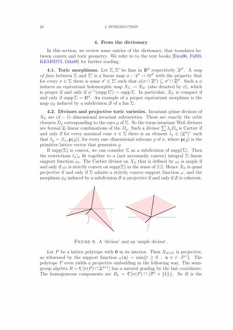
Let P be a lattice polytope with 0 in its interior. Then XN (P ) is projective,as witnessed by the support function ω(x) = mint ≥ 0 : x ∈ t · P∨. Thepolytope P even yields a projective embedding in the following way. The semi-group algebra R = C[σ(P ) ∩ Zd+1] has a natural grading by the last coordinate.The homogeneous components are Rk = C[σ(P ) ∩ (Zd × k)]. So R is the
4. FROM THE DICTIONARY 21
quotient of a polynomial ring by a homogeneously generated ideal, and we haveXN (P )
∼= Proj(R). The dimension of Rk is just Ehr(P, k), and thus the degreeof this embedding is (dim P )! times the leading coefficient of Ehr(P, k), which isthe normalized volume of P .
P × 1
2P × 2
3P × 3
Figure 9. The grading of C[σ(P ) ∩ Zd+1].

22 I. INTRODUCTION
CHAPTER II
Lattice width of empty simplices
1. Introduction
Geometric intuition may suggest that an empty lattice simplex must be “flat”in at least one direction, and if it is not “very flat,” then its volume must bebounded. The concepts of “flat” and “very flat” are made precise using thenotion of lattice width reviewed below. A “flat” simplex will be one whose latticewidth is bounded by a certain constant w(d) that depends only on the dimension,and it will be called “not very flat” if its lattice width is greater than anotherconstant w(d− 1). Using these concepts, we discuss in this chapter the (partial)validity of the geometric intuition.
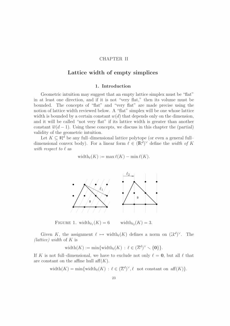
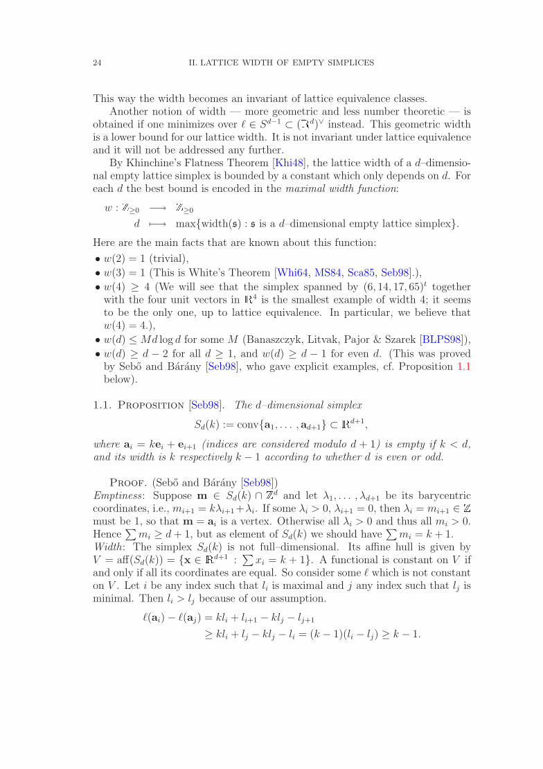
Let K ⊆ Rd be any full–dimensional lattice polytope (or even a general full–dimensional convex body). For a linear form ` ∈ (Rd)∨ define the width of Kwith respect to ` as
width`(K) := max `(K) − min `(K).
s
`1
`2
s
Figure 1. width`1(K) = 6 width`2(K) = 3.
Given K, the assignment ` 7→ width`(K) defines a norm on (Rd)∨. The(lattice) width of K is
width(K) := minwidth`(K) : ` ∈ (Zd)∨ r 0.If K is not full–dimensional, we have to exclude not only ` = 0, but all ` thatare constant on the affine hull aff(K).
width(K) = minwidth`(K) : ` ∈ (Zd)∨, ` not constant on aff(K).
23
24 II. LATTICE WIDTH OF EMPTY SIMPLICES
This way the width becomes an invariant of lattice equivalence classes.Another notion of width — more geometric and less number theoretic — is
obtained if one minimizes over ` ∈ Sd−1 ⊂ (Rd)∨ instead. This geometric widthis a lower bound for our lattice width. It is not invariant under lattice equivalenceand it will not be addressed any further.
By Khinchine’s Flatness Theorem [Khi48], the lattice width of a d–dimensio-nal empty lattice simplex is bounded by a constant which only depends on d. Foreach d the best bound is encoded in the maximal width function:
w : Z≥0 −→ Z≥0
d 7−→ maxwidth(s) : s is a d–dimensional empty lattice simplex.Here are the main facts that are known about this function:
• w(2) = 1 (trivial),
• w(3) = 1 (This is White’s Theorem [Whi64, MS84, Sca85, Seb98].),
• w(4) ≥ 4 (We will see that the simplex spanned by (6, 14, 17, 65)t togetherwith the four unit vectors in R4 is the smallest example of width 4; it seemsto be the only one, up to lattice equivalence. In particular, we believe thatw(4) = 4.),
• w(d) ≤ Md log d for some M (Banaszczyk, Litvak, Pajor & Szarek [BLPS98]),
• w(d) ≥ d − 2 for all d ≥ 1, and w(d) ≥ d − 1 for even d. (This was provedby Sebo and Barany [Seb98], who gave explicit examples, cf. Proposition 1.1below).
1.1. Proposition [Seb98]. The d–dimensional simplex
Sd(k) := conva1, . . . , ad+1 ⊂ Rd+1,
where ai = kei + ei+1 (indices are considered modulo d + 1) is empty if k < d,and its width is k respectively k − 1 according to whether d is even or odd.
Proof. (Sebo and Barany [Seb98])Emptiness : Suppose m ∈ Sd(k) ∩ Zd and let λ1, . . . , λd+1 be its barycentriccoordinates, i.e., mi+1 = kλi+1 +λi. If some λi > 0, λi+1 = 0, then λi = mi+1 ∈ Zmust be 1, so that m = ai is a vertex. Otherwise all λi > 0 and thus all mi > 0.Hence
∑mi ≥ d + 1, but as element of Sd(k) we should have
∑mi = k + 1.
Width: The simplex Sd(k) is not full–dimensional. Its affine hull is given byV = aff(Sd(k)) = x ∈ Rd+1 :
∑xi = k + 1. A functional is constant on V if
and only if all its coordinates are equal. So consider some ` which is not constanton V . Let i be any index such that li is maximal and j any index such that lj isminimal. Then li > lj because of our assumption.
`(ai) − `(aj) = kli + li+1 − klj − lj+1
≥ kli + lj − klj − li = (k − 1)(li − lj) ≥ k − 1.
1. INTRODUCTION 25
Equality can only hold if li − lj = 1 and for every maximal li, li+1 is minimal andvice versa, i.e., if ±` = (l, l + 1, l, l + 1, . . . , l, l + 1) for some l. But this can onlyhappen if d + 1 is even.
Imre Barany (personal communication 1997) related the volume of an emptylattice simplex to its width. He conjectured that the only way an empty simplexcan have arbitrarily high volume is that it is flat like a pancake. More precisely,he claimed that in every fixed dimension the volume of empty lattice simplices ofwidth ≥ 2 is bounded, or equivalently, there are only finitely many equivalenceclasses of such simplices. We will see that this is false in dimensions d ≥ 4. Eventhe weaker conjecture that there are only finitely many different empty latticesimplices of width larger than w(d − 1) is not true for d ≥ 4. However, we offera new guess for a finiteness result in Conjecture 2.7.
26 II. LATTICE WIDTH OF EMPTY SIMPLICES
2. Adding one dimension
The examples in Section 3 of empty 4–simplices of width greater than 1 to-gether with the following proposition show that Barany’s pancake conjecture doesnot hold in dimension d ≥ 5.
2.1. Proposition. Let d ≥ 3. Every empty (d−1)–dimensional lattice simplexs ⊂ Rd is a facet of infinitely many pairwise non–equivalent empty d–dimensionallattice simplices s ⊂ Rd that have at least the same width, width(s) ≥ width(s).
2.2. Corollary. The maximal width function is monotone: w(d) ≥ w(d − 1).¤
2.3. Corollary. For all d ≥ 3, there are infinitely many equivalence classesof d–dimensional empty lattice simplices of width ≥ w(d − 1). ¤
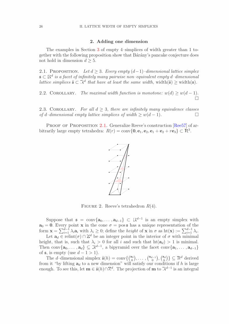
Proof of Proposition 2.1. Generalize Reeve’s construction [Ree57] of ar-bitrarily large empty tetrahedra: R(r) = conv0, e1, e2, e1 + e2 + re3 ⊂ R3.
Figure 2. Reeve’s tetrahedron R(4).
Suppose that s = conva0, . . . , ad−1 ⊂ Rd−1 is an empty simplex witha0 = 0. Every point x in the cone σ = pos s has a unique representation of theform x =
∑d−1i=1 λiai with λi ≥ 0; define the height of x in σ as ht(x) :=
∑d−1i=1 λi.
Let ad ∈ relint(σ) ∩ Zd be an integer point in the interior of σ with minimalheight, that is, such that λi > 0 for all i and such that ht(ad) > 1 is minimal.Then conva0, . . . , ad ⊆ Rd−1, a bipyramid over the facet conva1, . . . , ad−1of s, is empty (use d − 1 > 1).
The d–dimensional simplex s(h) = conv(a0
0
), . . . ,
(ad−1
0
),(ad
h
) ⊆ Rd derived
from it “by lifting ad to a new dimension” will satisfy our conditions if h is largeenough. To see this, let m ∈ s(h)∩Zd. The projection of m to Rd−1 is an integral
2. ADDING ONE DIMENSION 27
point which lies in the bipyramid, so it must be one of the points a0, . . . , ad. Butthe only points of s(h) with such a projection are the vertices.
Any functional ` ∈ (Zd)∨ has the same values on the first d vertices ofs(h) as its restriction `′ to Rd−1 takes on the vertices of s. Hence, we havewidth`(s) ≥ width`′(s). This shows that width`(s)(h) ≥ width(s), unless `′ is zero.In this last case ` has to be an integer multiple of the d–th coordinate function,which takes the values 0 and h on the vertices of s(h). This establishes thatwidth(s)(h) ≥ minh, width(s).For a sharper analysis of the situation we introduce the following concept.
2.4. Definition. A lattice simplex without interior lattice points and with atleast one empty facet is called almost empty. Let w(d) be the maximal widthfunction for almost empty simplices.
The following Proposition in particular shows that w(d) ≤ w(d + 1) is finite.
2.5. Proposition. For any (d − 1)–dimensional almost empty simplex thereare infinitely many pairwise non–equivalent d–dimensional empty simplices of atleast the same width.
As a special case of Proposition 2.5, we get the following infinite family of4–dimensional empty lattice simplices of width 2 > w(3), which disproves thepancake conjecture in dimension 4. For this, write
s[m] := conve1, e2, . . . , ed,m
,
to denote the convex hull of the standard unit vectors together with one additionalvector m ∈ Zd. We always assume that
∑di=1 mi =: D + 1 > 1. (D is the
determinant of s[m].)
2.6. Proposition. For every determinant D ≥ 8, the 4–simplex s[(2, 2, 3, D−6)t], which is the convex hull of the columns of
1 0 0 0 20 1 0 0 20 0 1 0 30 0 0 1 D − 6
,
has width 2. It is empty if and only if gcd(D, 6) = 1. ¤
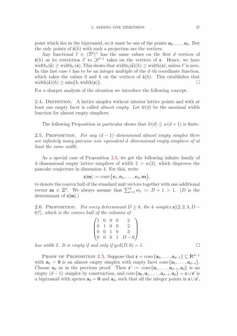
Proof of Proposition 2.5. Suppose that s = conva0, . . . , ad−1 ⊆ Rd−1
with a0 = 0 is an almost empty simplex with empty facet conva1, . . . , ad−1.Choose ad as in the previous proof. Then s′ := conva1, . . . , ad−1, ad is anempty (d− 1)–simplex by construction, and conva0, a1, . . . , ad−1, ad = s∪ s′ isa bipyramid with apexes a0 = 0 and ad, such that all the integer points in s∪ s′,
28 II. LATTICE WIDTH OF EMPTY SIMPLICES
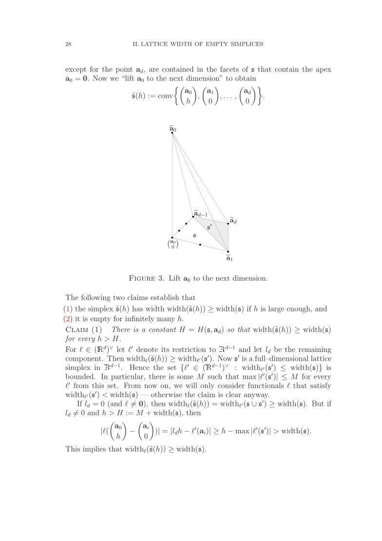
except for the point ad, are contained in the facets of s that contain the apexa0 = 0. Now we “lift a0 to the next dimension” to obtain
s(h) := conv
(a0
h
),
(a1
0
), . . . ,
(ad
0
).
(a0
0
)ad−1
a0
s
a1
ads′
Figure 3. Lift a0 to the next dimension.
The following two claims establish that
(1) the simplex s(h) has width width(s(h)) ≥ width(s) if h is large enough, and
(2) it is empty for infinitely many h.
Claim (1) There is a constant H = H(s, ad) so that width(s(h)) ≥ width(s)for every h > H.
For ` ∈ (Rd)∨ let `′ denote its restriction to Rd−1 and let ld be the remainingcomponent. Then width`(s(h)) ≥ width`′(s
′). Now s′ is a full–dimensional latticesimplex in Rd−1. Hence the set `′ ∈ (Rd−1)∨ : width`′(s
′) ≤ width(s) isbounded. In particular, there is some M such that max |`′(s′)| ≤ M for every`′ from this set. From now on, we will only consider functionals ` that satisfywidth`′(s
′) < width(s) — otherwise the claim is clear anyway.If ld = 0 (and ` 6= 0), then width`(s(h)) = width`′(s ∪ s′) ≥ width(s). But if
ld 6= 0 and h > H := M + width(s), then
|`((a0
h
)−
(ai
0
))| = |ldh − `′(ai)| ≥ h − max |`′(s′)| > width(s).
This implies that width`(s(h)) ≥ width(s).
2. ADDING ONE DIMENSION 29
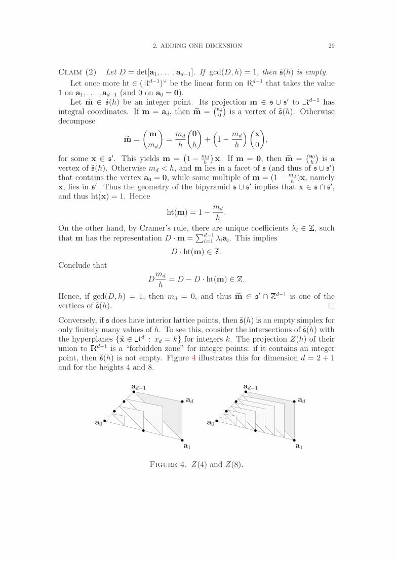
Claim (2) Let D = det[a1, . . . , ad−1]. If gcd(D, h) = 1, then s(h) is empty.
Let once more ht ∈ (Rd−1)∨ be the linear form on Rd−1 that takes the value1 on a1, . . . , ad−1 (and 0 on a0 = 0).
Let m ∈ s(h) be an integer point. Its projection m ∈ s ∪ s′ to Rd−1 hasintegral coordinates. If m = ad, then m =
(ad
0
)is a vertex of s(h). Otherwise
decompose
m =
(m
md
)=
md
h
(0
h
)+
(1 − md
h
) (x
0
),
for some x ∈ s′. This yields m =(1 − md
h
)x. If m = 0, then m =
(a0
h
)is a
vertex of s(h). Otherwise md < h, and m lies in a facet of s (and thus of s ∪ s′)that contains the vertex a0 = 0, while some multiple of m = (1 − md
h)x, namely
x, lies in s′. Thus the geometry of the bipyramid s ∪ s′ implies that x ∈ s ∩ s′,and thus ht(x) = 1. Hence
ht(m) = 1 − md
h.
On the other hand, by Cramer’s rule, there are unique coefficients λi ∈ Z, suchthat m has the representation D · m =
∑d−1i=1 λiai. This implies
D · ht(m) ∈ Z.
Conclude that
Dmd
h= D − D · ht(m) ∈ Z.
Hence, if gcd(D, h) = 1, then md = 0, and thus m ∈ s′ ∩ Zd−1 is one of thevertices of s(h).
Conversely, if s does have interior lattice points, then s(h) is an empty simplex foronly finitely many values of h. To see this, consider the intersections of s(h) withthe hyperplanes x ∈ Rd : xd = k for integers k. The projection Z(h) of theirunion to Rd−1 is a “forbidden zone” for integer points: if it contains an integerpoint, then s(h) is not empty. Figure 4 illustrates this for dimension d = 2 + 1and for the heights 4 and 8.
ad
a1
ad−1
a0
ad
a1
ad−1
a0
Figure 4. Z(4) and Z(8).
30 II. LATTICE WIDTH OF EMPTY SIMPLICES
You can see that Z(h) contains an inner parallel body of s that grows withh and which completely fills the interior of s for h → ∞. So any fixed interiorpoint of s lies in Z(h) if h is large enough.
As promised, we conclude this section with a new modified finiteness conjec-ture. Given some huge wide empty simplex s ⊂ Rd, we can always suppose thatthe smallest facet s lies in Rd−1. Then our simplex is of the form s = s(h) forsome huge h = det(s)/ det(s). One is tempted to believe that h is large enoughto (1): exclude interior lattice points from the projection of s to Rd−1, and (2):assure that any functional that realizes the width must live in Rd−1.
2.7. Conjecture. For every d ≥ 2, there are only finitely many equivalenceclasses of empty d–simplices whose width is greater than w(d − 1), the greatestwidth that can be achieved in dimension d − 1 by almost empty simplices.
This includes the conjecture that the maximal width of the bipyramids in-volved cannot be greater than w.
3. COMPUTER SEARCH IN DIMENSION 4 31
3. Computer search in dimension 4
As already mentioned, 3–dimensional empty simplices always have width 1.The first examples of width 2 simplices in dimensions 4 and 5 were given byUwe Wessels [Wes89]. In this section we describe the search for wide empty4–simplices. The strategy is the following:
1. enumerate all equivalence classes of (possibly) empty simplices,2. check whether or not the simplex is in fact empty, and3. if so, calculate the width.
This relies on the two known results 3.1 and 3.3.
3.1. Theorem [Wes89]. Every empty 4–simplex has at least two unimodularfacets. In particular, every such simplex is equivalent to a simplex of the forms[m]. ¤
(The analogous statement is false in higher dimensions. For example, thesimplex in R5 given by the columns of
0 1 0 0 1 20 0 1 0 1 30 0 0 1 1 40 0 0 0 6 00 0 0 0 0 9
,
is empty, without any unimodular facet [Wes89, p. 21].)We can further restrict our search for empty simplices, as follows.
3.2. Lemma. The simplex s[m] is lattice equivalent to s[m+Dε], where ε ∈ Zd
is any vector with vanishing coordinate sum. In particular, s[m] is equivalent tosome s[m′] with ‖m′‖∞ ≤ D. Furthermore, any orientation preserving latticeequivalence which fixes the vertices ei, is of this type. ¤
Given a determinant D, enumerate sorted 4–tuples m with∑
mi = D + 1 inthe range given by Lemma 3.2. Then test emptiness by the following criterion,which is (up to the range restriction k ≤ D/2) due to Herb Scarf.
3.3. Theorem [Sca85]. The lattice simplex s[m] = conve1, . . . , ed,m of de-
terminant D :=∑d
i=1 mi − 1 > 0 is empty if and only if
d∑i=1
⌈kmi
D
⌉> k + 1(3.1)
holds for all integers k in the range 1 ≤ k ≤ D/2.
32 II. LATTICE WIDTH OF EMPTY SIMPLICES
Proof. Observe thatd∑
i=1
⌈kmi
D
⌉≥ k + 1
always holds, since∑d
i=1
⌈kmi
D
⌉≥
∑di=1
kmi
D= k
D
∑di=1 mi = kD+1
D> k.
Also it is readily checked that∑d
i=1 xi ≥ 1 together with the inequalities∑di=1 xi − 1
Dmj ≤ xj <
∑di=1 xi − 1
Dmj + 1(3.2)
describes the set s r e1, . . . , ed: the weak inequalities describe s and the strictones cut off the vertices ei.
If there is a lattice point x in s r e1, . . . , ed, set k = k(x) :=∑d
i=1 xi − 1.Then by (3.2) x must have the coordinates
xj =
⌈kmj
D
⌉.(3.3)
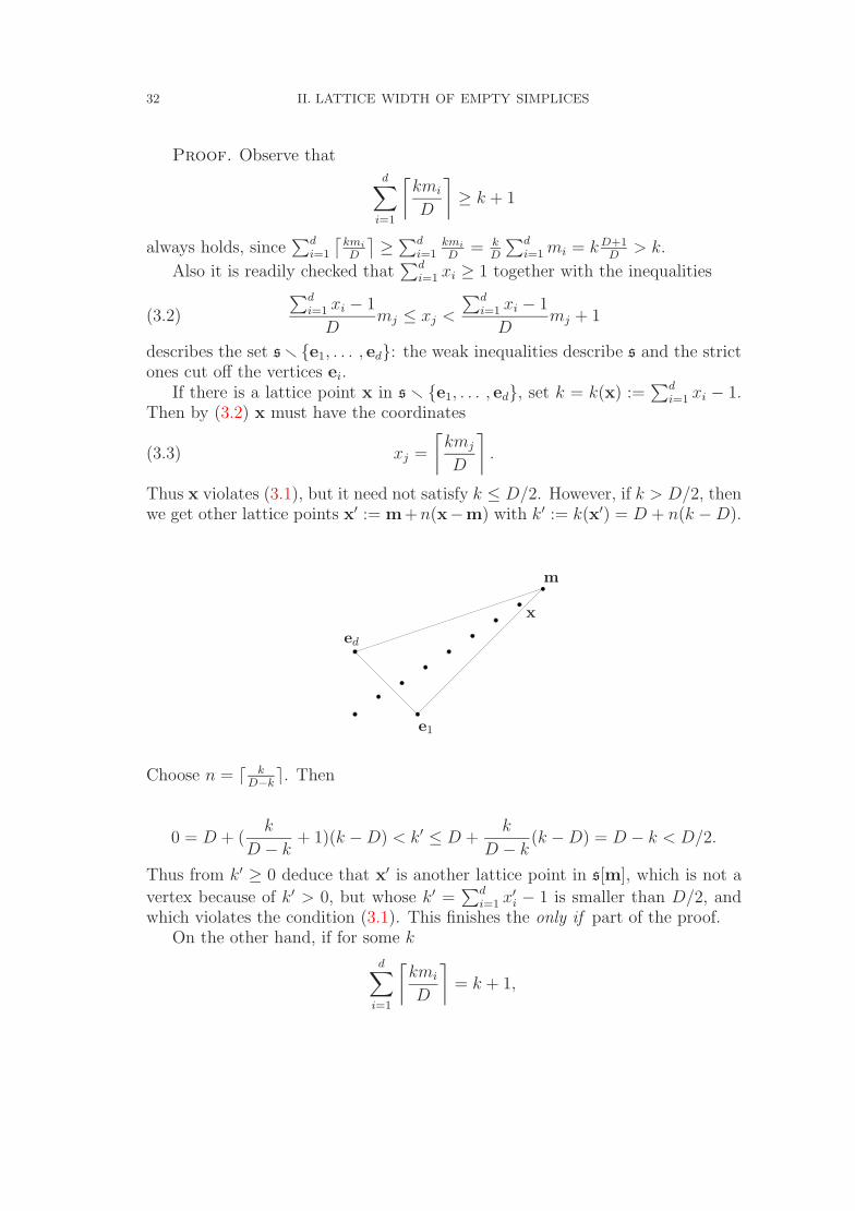
Thus x violates (3.1), but it need not satisfy k ≤ D/2. However, if k > D/2, thenwe get other lattice points x′ := m+n(x−m) with k′ := k(x′) = D + n(k − D).
e1
m
ed
x
Choose n = d kD−k
e. Then
0 = D + (k
D − k+ 1)(k − D) < k′ ≤ D +
k
D − k(k − D) = D − k < D/2.
Thus from k′ ≥ 0 deduce that x′ is another lattice point in s[m], which is not a
vertex because of k′ > 0, but whose k′ =∑d
i=1 x′i − 1 is smaller than D/2, and
which violates the condition (3.1). This finishes the only if part of the proof.On the other hand, if for some k
d∑i=1
⌈kmi
D
⌉= k + 1,
3. COMPUTER SEARCH IN DIMENSION 4 33
then the vector x given by (3.3) satisfies (3.2), and thus provides a lattice pointin s[m] which is not a vertex.
In principle, the width of a lattice simplex can be found by solving an integerprogram, as demonstrated by the following lemma.
3.4. Lemma. Let W be an upper bound for the width of the simplex s[m]. Thenwidth(s[m]) is the optimal value of the following minimization problem:
minimize w subject to
w0 ≤ li ≤ w0 + w for 1 ≤ i ≤ d,
w0 ≤∑d
i=1 limi ≤ w0 + w,∑di=1 liW
i−1 ≥ 1,
(3.4)
with integer variables w, w0, and li. (The values of the li–variables in an optimalsolution yield a linear functional that realizes the width.)
Proof. The width is defined to be the minimal solution to the first con-straints, excluding the zero solution (` = 0, w = w0 = 0). This solution is cut offby the last constraint. We have to see that some ` 6= 0 that realizes the widthof s[m] satisfies this last constraint. By replacing the li by their negatives, we canassure the left hand side of this constraint to be non–negative. If it were zero, thefirst non–zero li would have to be a multiple of W and some other lj would havethe opposite sign, with the effect that |`(ei) − `(ej)| = |li − lj| > |li| ≥ W .
An integer programming formulation as in Lemma 3.4 also shows that the widthof a general lattice simplex can be computed in polynomial time if the dimen-sion is fixed. (A different IP formulation was provided by Sebo [Seb98, § 5].)Somewhat surprisingly, our computational tests using CPLEX∗ showed that theinteger programs of Lemma 3.4 can indeed be solved fast and stably, providedthat W is not too large. We used this for an enumeration of 4–dimensional emptylattice simplices up to determinant D = 350, and also for tests in dimension 5.
However, for larger determinants a less sophisticated criterion proved to befaster. Namely, a simplex s[m] has lattice width greater than w if and only ifthere is no solution to
0 ≤ l′i ≤ w for 1 ≤ i ≤ d,∑di=1 l′imi (mod D) ≤ w,
(l′1, . . . , l′d) 6= (0, . . . , 0).
This is easily derived from the system (3.4) using the substitutions l′i := li − w0.Thus, to test e.g. whether a 4–dimensional simplex has width greater than 2,
∗CPLEX Linear Optimizer 4.0.8 with Mixed Integer & Barrier Solvers; c©CPLEX Opti-mization, Inc., 1989-1995
34 II. LATTICE WIDTH OF EMPTY SIMPLICES
one simply has to see whether there is one of the 34 − 1 = 80 different 4–tuples(l′1, . . . , l′4) ∈ 0, 1, 24 r 0 that satisfies the modular inequality
d∑i=1
l′imi (mod D) ≤ 2.
This method yields a complete list of empty 4–simplices s[m] that have a givendeterminant and width ≥ 3. In order to exclude multiple representatives ofthe same equivalence class, we have to develop an equivalence test. A latticeequivalence that maps s[m] to some s[m′] can either map m to m′ (then it isa transformation as in Lemma 3.2 followed by a permutation of coordinates) orit maps m to some ei. In the latter case, we can — again, up to coordinatepermutations — apply the following Lemma 3.5, to get a transformation thatfixes the ei.
3.5. Lemma. The facet conve1, e2, e3,m of s[m] is unimodular if and onlyif gcd(D,m4) = 1. In that case let p, q ∈ Z such that pm4 − qD = 1. Then theaffine map given by
x 7−→
1 + qm1 qm1 qm1 (q − p)m1
qm2 1 + qm2 qm2 (q − p)m2
qm3 qm2 1 + qm3 (q − p)m3
km4 − q km4 − q km4 − q p − q + k(m4 − D)
x −
qm1
qm2
qm3
km4 − q
(with k = q − p − 1) is lattice preserving and maps
e1 7−→ e1
e2 7−→ e2
e3 7−→ e3
e4 7−→ (−pm1,−pm2,−pm3, p + (p − q + 1)D)t
m 7−→ e4.
¤
The coordinate transformations can be ruled out by sorting the mi and theLemma 3.2 transformations by comparison of the moduli mi (mod D). Thefollowing theorem records our computational results, based on generation andtest of all equivalence classes of empty lattice simplices of determinant D ≤ 1000.It provides evidence for w(4) = 4 as well as for Conjecture 2.7.
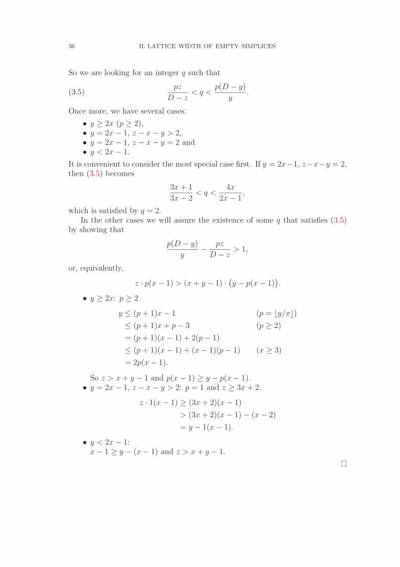
3. COMPUTER SEARCH IN DIMENSION 4 35
3.6. Theorem. Among the 4–dimensional empty lattice simplices of determi-nant D ≤ 1000,
• there are no simplices of width 5 or larger,
• there is a unique equivalence class of simplices of width 4 which is representedby the simplex s[(6, 14, 17, 65)t], whose determinant is D = 101,
• all simplices of width 3 have determinant D ≤ 179, where the (unique) smallestexample, of determinant D = 41, is represented by s[(−10, 4, 23, 25)t], and the(unique) example of determinant D = 179 is represented by s[(20, 36, 53, 71)t].
This result has been found independently by Fermigier and Kantor, and it wasconfirmed by Wahidi [Wah99].
If it were true that every empty 4–simplex of width 3 has determinant ≤ 179,it would follow that w(3) ≤ 2, the latter can be shown directly:
3.7. Proposition. The lattice width of any almost empty tetrahedron is atmost 2, i.e.,
w(3) = 2.
Proof. The almost empty tetrahedron s[(2, 2, 3)t] underlying Proposition 2.6shows that w(3) ≥ 2.
Suppose that there is an almost empty tetrahedron s of width ≥ 3. We firstbring it into normal form: Up to a unimodular transformation, s has vertices0, e1, e2, (x, y, z′)t with z′ ≥ 1 and 0 ≤ x, y < z′. If z′ ≤ x + y − 2, then (1, 1, 1)t
would be an interior point. Hence z′ ≥ x+y−1 and s is equivalent to s[(x, y, z)t]with z = z′ − x − y + 1 ≥ 0.
Let us suppose 0 ≤ x ≤ y ≤ z. Because of width(s) ≥ 3 we know that x ≥ 3,y − x ≥ 2, z − y ≥ 2 and |z − x − y| ≥ 2. From these inequalities we want todeduce that there is an interior lattice point. Therefore, observe that the latticepoint given by (3.3) is interior if and only if both inequalities in (3.2) are strict.In other words, we have to produce some k such that⌈
kx
D
⌉+
⌈ky
D
⌉+
⌈ky
D
⌉= k + 1,
and none of the three fractions is integral. There are two cases.
• z − x − y ≤ −2: (1, 1, 1)t is an interior point (k = 2).• z−x− y ≥ 2: Abbreviate p := by/xc. Then there is an integer q such that
(1, p, q)t is an interior point (k = p + q).
We still have to prove the second claim. It is equivalent to((p + q)x
D< 1 ⇐=
)(p + q)y
D< p and
(p + q)z
D< q.
36 II. LATTICE WIDTH OF EMPTY SIMPLICES
So we are looking for an integer q such that
pz
D − z< q <
p(D − y)
y.(3.5)
Once more, we have several cases:
• y ≥ 2x (p ≥ 2),• y = 2x − 1, z − x − y > 2,• y = 2x − 1, z − x − y = 2 and• y < 2x − 1.
It is convenient to consider the most special case first. If y = 2x−1, z−x−y = 2,then (3.5) becomes
3x + 1
3x − 2< q <
4x
2x − 1,
which is satisfied by q = 2.In the other cases we will assure the existence of some q that satisfies (3.5)
by showing that
p(D − y)
y− pz
D − z> 1,
or, equivalently,
z · p(x − 1) > (x + y − 1) ·(y − p(x − 1)
).
• y ≥ 2x: p ≥ 2
y ≤ (p + 1)x − 1 (p = by/xc)≤ (p + 1)x + p − 3 (p ≥ 2)
= (p + 1)(x − 1) + 2(p − 1)
≤ (p + 1)(x − 1) + (x − 1)(p − 1) (x ≥ 3)
= 2p(x − 1).
So z > x + y − 1 and p(x − 1) ≥ y − p(x − 1).• y = 2x − 1, z − x − y > 2: p = 1 and z ≥ 3x + 2.
z · 1(x − 1) ≥ (3x + 2)(x − 1)
> (3x + 2)(x − 1) − (x − 2)
= y − 1(x − 1).
• y < 2x − 1:x − 1 ≥ y − (x − 1) and z > x + y − 1.
3. COMPUTER SEARCH IN DIMENSION 4 37
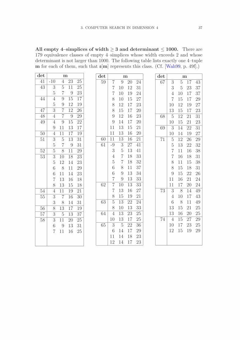
All empty 4–simplices of width ≥ 3 and determinant ≤ 1000. There are179 equivalence classes of empty 4–simplices whose width exceeds 2 and whosedeterminant is not larger than 1000. The following table lists exactly one 4–tuplem for each of them, such that s[m] represents this class. (Cf. [Wah99, p. 49f].)
det m41 -10 4 23 2543 3 5 11 25
5 7 9 2344 4 9 15 17
5 9 12 1947 3 7 12 2648 4 7 9 2949 4 9 15 22
9 11 13 1750 4 11 17 1951 3 5 13 31
5 7 9 3152 5 8 11 2953 3 10 18 23
5 12 14 236 8 11 296 11 14 237 13 16 188 13 15 18
54 4 11 19 2155 3 7 16 30
3 8 14 3156 8 13 17 1957 3 5 13 3758 3 11 20 25
6 9 13 317 11 16 25
det m59 7 9 20 24
7 10 12 317 10 19 248 10 15 278 12 17 238 15 17 209 12 16 239 14 17 20
11 13 15 2111 13 16 20
60 11 13 16 2161 -9 3 27 41
3 5 13 414 7 18 335 7 18 326 8 11 376 9 13 347 9 13 33
62 7 10 13 337 13 16 278 15 19 21
63 5 13 22 248 10 13 33
64 4 13 23 2510 13 17 25
65 3 5 22 366 14 17 29
11 14 18 2312 14 17 23
det m67 3 5 17 43
3 5 23 374 10 17 377 15 17 29
10 12 19 2713 15 17 23
68 5 12 21 3110 15 21 23
69 3 14 22 3110 14 19 27
71 5 12 26 295 13 22 327 11 16 387 16 18 318 11 15 388 15 18 319 15 22 26
11 16 21 2411 17 20 24
73 3 8 14 494 10 17 436 8 11 49
13 15 21 2513 16 20 25
74 4 15 27 2910 17 23 2512 15 19 29
38 II. LATTICE WIDTH OF EMPTY SIMPLICES
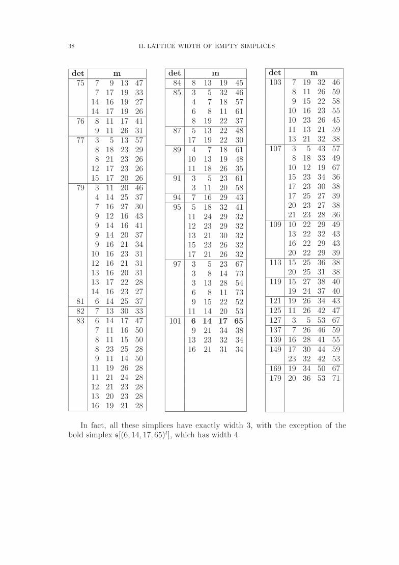
det m75 7 9 13 47
7 17 19 3314 16 19 2714 17 19 26
76 8 11 17 419 11 26 31
77 3 5 13 578 18 23 298 21 23 26
12 17 23 2615 17 20 26
79 3 11 20 464 14 25 377 16 27 309 12 16 439 14 16 419 14 20 379 16 21 34
10 16 23 3112 16 21 3113 16 20 3113 17 22 2814 16 23 27
81 6 14 25 3782 7 13 30 3383 6 14 17 47
7 11 16 508 11 15 508 23 25 289 11 14 50
11 19 26 2811 21 24 2812 21 23 2813 20 23 2816 19 21 28
det m84 8 13 19 4585 3 5 32 46
4 7 18 576 8 11 618 19 22 37
87 5 13 22 4817 19 22 30
89 4 7 18 6110 13 19 4811 18 26 35
91 3 5 23 613 11 20 58
94 7 16 29 4395 5 18 32 41
11 24 29 3212 23 29 3213 21 30 3215 23 26 3217 21 26 32
97 3 5 23 673 8 14 733 13 28 546 8 11 739 15 22 52
11 14 20 53101 6 14 17 65
9 21 34 3813 23 32 3416 21 31 34
det m103 7 19 32 46
8 11 26 599 15 22 58
10 16 23 5510 23 26 4511 13 21 5913 21 32 38
107 3 5 43 578 18 33 49
10 12 19 6715 23 34 3617 23 30 3817 25 27 3920 23 27 3821 23 28 36
109 10 22 29 4913 22 32 4316 22 29 4320 22 29 39
113 15 25 36 3820 25 31 38
119 15 27 38 4019 24 37 40
121 19 26 34 43125 11 26 42 47127 3 5 53 67137 7 26 46 59139 16 28 41 55149 17 30 44 59
23 32 42 53169 19 34 50 67179 20 36 53 71
In fact, all these simplices have exactly width 3, with the exception of thebold simplex s[(6, 14, 17, 65)t], which has width 4.
CHAPTER III
Crepant resolutions of toric l.c.i.–singularities
1. Introduction
1.1. Motivation. In the past two decades crepant birational morphismswere mainly used in algebraic geometry to reduce the canonical singularitiesof algebraic d–folds, d ≥ 3, to Q–factorial terminal singularities, and to treatminimal models in high dimensions. From the late eighties onwards, crepant full
desingularizations Y → Y of projective varieties Y with trivial dualizing sheafand mild singularities (like quotient or toroidal singularities) play also a crucialrole in producing Calabi–Yau manifolds , which serve as internal target spaces fornon–linear super–symmetric sigma models in the framework of physical string–theory. This explains the recent mathematical interest in both local and globalversions of the existence problem of smooth birational models of such Y ’s.
Locally, the high–dimensional McKay correspondence (cf. [IR94, Rei]) for theunderlying spaces Cd/G, G ⊂ SL(d,C), of Gorenstein quotient singularities wasproved by Batyrev [Bat99, Theorem 8.4]. It states that the following two quan-tities are equal:
• the ranks of the non–trivial (=even) cohomology groups H2k(X,C) of the
overlying spaces X of crepant, full desingularizations X → X = Cd/G on theone hand,
• the number of conjugacy classes of G having the weight (also called “age”) kon the other.
Moreover, a one–to–one correspondence of McKay–type is also true for torus–
equivariant, crepant, full desingularizations X → X = Uσ of the underlyingspaces of Gorenstein toric singularities [BD96, §4]. Again, the non–trivial (even)
cohomology groups of the X’s have the “expected” dimensions, which in this caseare determined by the Ehrhart polynomials of the corresponding lattice polytopes(cf. Chapter IV). Thus in both situations the ranks of the cohomology groups of
X’s turn out to be independent of the particular choice of a crepant resolution.Also in both situations, a crepant resolution always exists if d ≤ 3, but not ingeneral: for d ≥ 4 there are, for instance, lots of terminal Gorenstein singularitiesin both classes, such as the toric quotient singularities Uσ(s) for empty simplicess (cf. Chapter II).
39
40 III. CREPANT RESOLUTIONS OF TORIC L.C.I.–SINGULARITIES
We believe that a purely algebraic, sufficient condition for the existence ofprojective, crepant, full resolutions in all dimensions is to require from our singu-larities to be, in addition, local complete intersections (l.c.i.’s). In the toric cat-egory, this conjecture was verified for Abelian quotient singularities in [DHZ98b]via a Theorem by Kei–ichi Watanabe [Wat80]. (For non–Abelian groups acting onCd, it remains open.) Furthermore, Dais, Henk and Ziegler [DHZ98b, cf. §8(iii)]asked for geometric analogues of the joins and dilations occuring in their reduc-tion theorem also for toric non–quotient l.c.i.–singularities. As we shall see below,such a characterization (in a somewhat different context) is indeed possible bymaking use of another beautiful classification theorem due to Haruhisa Nakajima[Nak86], which generalizes Watanabe’s results to the entire class of toric l.c.i.’s.Based on this classification we prove the following:
1.1. Theorem. The underlying spaces of all toric l.c.i.–singularities admit to-rus–equivariant, projective, crepant, full resolutions (i.e., smooth minimal mod-els) in all dimensions.
Families of Gorenstein non–l.c.i. toric singularities that have such special fullresolutions seem to be very rare. This problem is discussed in [DHH98, DHb] forcertain families of Abelian quotient non–l.c.i. singularities.
1.2. Crepant resolutions via triangulations. The divisor KΣ = −∑
D%
on XΣ is canonical. The affine piece Uσ is Gorenstein if and only if the canonicaldivisor is Cartier, i.e., there is an integral linear functional `σ that takes thevalue −1 on all primitive ray generating lattice vectors p(%) (cf. I.4.2). Deduce:
1.2. Proposition. XΣ is Gorenstein if and only if every cone in Σ is equivalentto a cone spanned by some lattice polytope.
Recall that a subdivision S of a fan Σ induces a proper birational morphismφS : XS → XΣ. In this situation, the affine pieces Uσ that cover the overlyingspace XS are smooth if and only if the σ are unimodular:
1.3. Proposition. The morphism φS : XS → XΣ is a full desingularization ifand only if S is a unimodular triangulation.
Also, φS is projective if and only if S is a coherent subdivision of Σ. Pro-jective full desingularizations always exist for any XΣ (see [KKMSD73, §I.2]).Nevertheless, we ask in this section about conditions under which such φS are, inaddition, crepant. This is a local question that only makes sense if both XΣ andXS are (Q–)Gorenstein. So, locally, suppose that the cone σ = σ(P ) ⊂ Rd+1 isspanned by a lattice polytope P ⊂ Rd. Then the canonical divisor KUσ (withO(KUσ) trivial) is defined by the linear functional x 7→ −xd+1. The pull back
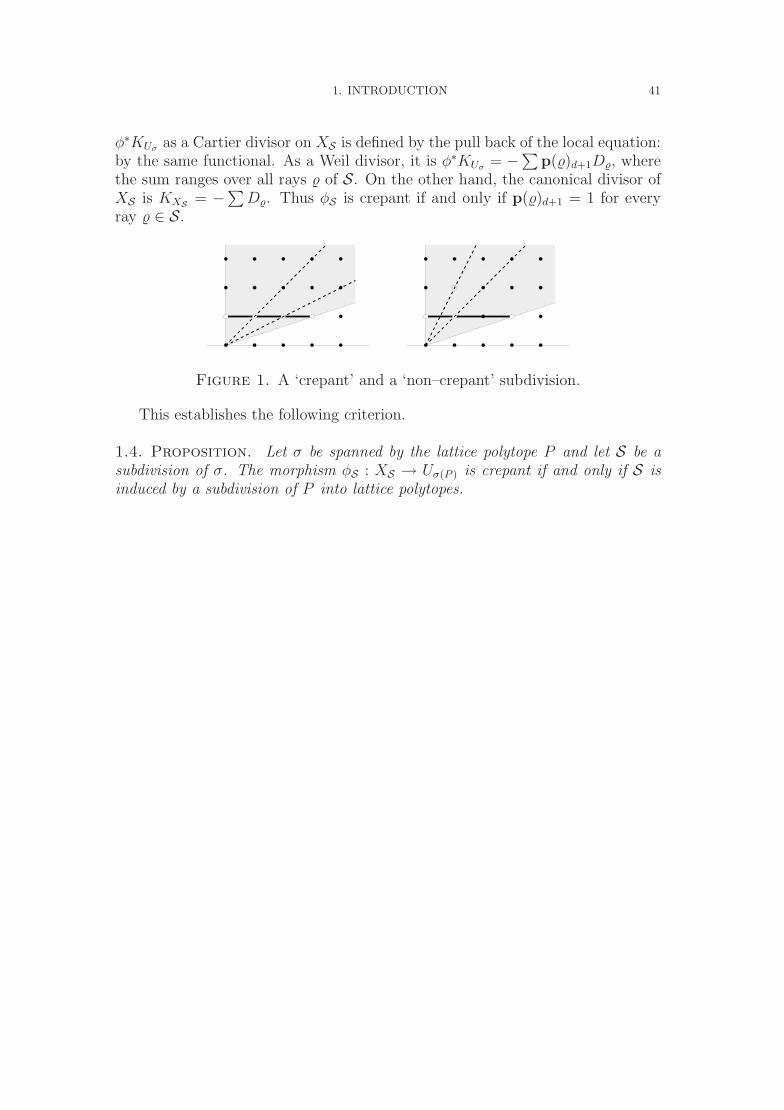
1. INTRODUCTION 41
φ∗KUσ as a Cartier divisor on XS is defined by the pull back of the local equation:by the same functional. As a Weil divisor, it is φ∗KUσ = −
∑p(%)d+1D%, where
the sum ranges over all rays % of S. On the other hand, the canonical divisor ofXS is KXS = −
∑D%. Thus φS is crepant if and only if p(%)d+1 = 1 for every
ray % ∈ S.
Figure 1. A ‘crepant’ and a ‘non–crepant’ subdivision.
This establishes the following criterion.
1.4. Proposition. Let σ be spanned by the lattice polytope P and let S be asubdivision of σ. The morphism φS : XS → Uσ(P ) is crepant if and only if S isinduced by a subdivision of P into lattice polytopes.
42 III. CREPANT RESOLUTIONS OF TORIC L.C.I.–SINGULARITIES
2. Proof of the Main Theorem
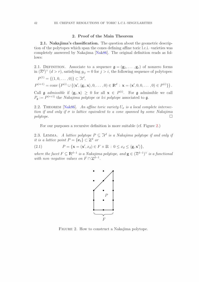
2.1. Nakajima’s classification. The question about the geometric descrip-tion of the polytopes which span the cones defining affine toric l.c.i.–varieties wascompletely answered by Nakajima [Nak86]. The original definition reads as fol-lows:
2.1. Definition. Associate to a sequence g = (g1, . . . ,gr) of nonzero formsin (Zd)∨ (d > r), satisfying gij = 0 for j > i, the following sequence of polytopes:
P (1) = (1, 0, . . . , 0) ⊂ Rd,
P (i+1) = conv(P (i) ∪ (x′, 〈gi,x〉, 0, . . . , 0) ∈ Rd : x = (x′, 0, 0, . . . , 0) ∈ P (i)
).
Call g admissible if 〈gi,x〉 ≥ 0 for all x ∈ P (i). For g admissible we callPg := P (r+1) the Nakajima polytope or lci polytope associated to g.
2.2. Theorem [Nak86]. An affine toric variety Uσ is a local complete intersec-tion if and only if σ is lattice equivalent to a cone spanned by some Nakajimapolytope. ¤
For our purposes a recursive definition is more suitable (cf. Figure 2.)
2.3. Lemma. A lattice polytope P ⊆ Rd is a Nakajima polytope if and only ifit is a lattice point P = e1 ⊂ Zd or
P = x = (x′, xd) ∈ F ×R : 0 ≤ xd ≤ 〈g,x′〉,(2.1)
where the facet F ⊆ Rd−1 is a Nakajima polytope, and g ∈ (Zd−1)∨ is a functionalwith non–negative values on F ∩ Zd−1.
P
F
Figure 2. How to construct a Nakajima polytope.
2. PROOF OF THE MAIN THEOREM 43
Proof. Let g be an admissible sequence. Then the corresponding Nakajimapolytope Pg has the following description by inequalities:
Pg = x ∈ Rd : x1 = 1 and 0 ≤ xi+1 ≤ 〈gi,x〉 for 1 ≤ i ≤ d − 1,(2.2)
so that Pg can be reconstructed from the facet F = Pg′ and g = gr, where g′
is the truncated sequence (g1, . . . ,gr−1). Conversely, given the situation (2.1),F is some Pg′ . Then we can append g to g′ and obtain an admissible sequencefor P .
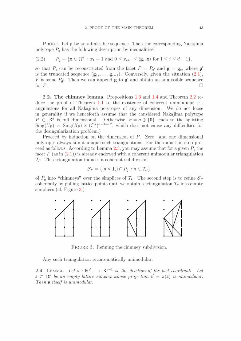
2.2. The chimney lemma. Propositions 1.3 and 1.4 and Theorem 2.2 re-duce the proof of Theorem 1.1 to the existence of coherent unimodular tri-angulations for all Nakajima polytopes of any dimension. We do not loosein generality if we henceforth assume that the considered Nakajima polytopeP ⊂ Rd is full–dimensional. (Otherwise, σ = σ ⊕ 0 leads to the splittingSing(UP ) = Sing(Xσ) × (C∗)d−dim P , which does not cause any difficulties forthe desingularization problem.)
Proceed by induction on the dimension of P . Zero– and one–dimensionalpolytopes always admit unique such triangulations. For the induction step pro-ceed as follows: According to Lemma 2.3, you may assume that for a given Pg thefacet F (as in (2.1)) is already endowed with a coherent unimodular triangulationTF . This triangulation induces a coherent subdivision
SP = (s ×R) ∩ Pg : s ∈ TF
of Pg into “chimneys” over the simplices of TF . The second step is to refine SP
coherently by pulling lattice points until we obtain a triangulation TP into emptysimplices (cf. Figure 3.)
Figure 3. Refining the chimney subdivision.
Any such triangulation is automatically unimodular:
2.4. Lemma. Let π : Rd −→ Rd−1 be the deletion of the last coordinate. Lets ⊂ Rd be an empty lattice simplex whose projection s′ = π(s) is unimodular.Then s itself is unimodular.
44 III. CREPANT RESOLUTIONS OF TORIC L.C.I.–SINGULARITIES
Proof. We can assume that s is full–dimensional. After a lattice equivalenceof Rd−1 we can suppose that s′ =Md−1 is the standard (d − 1)–simplex. After atranslation in the last coordinate, s contains the origin. Now we can shift the linesπ−1(ei) independently such that we finally obtain a simplex with non–negativelast coordinate that contains Md−1 ×0. The fact that s is empty implies thatthe additional vertex has last coordinate 1.
Proof of Theorem 1.1. By construction, all simplices of TP are emptybecause P ∩ Zd coincides with the set of vertices of TP (we pulled them all.)Since their projections under π are the unimodular simplices of TF , they havethemselves to be unimodular by the Chimney Lemma 2.4.
3. APPLICATIONS 45
3. Applications
3.1. Computing Betti numbers. This paragraph is, in a sense, a sneakpreview of Chapter IV. We are interested in the rational cohomology groups ofthe crepant resolutions XT as constructed in the previous section. They do infact not depend on the particular choice of a triangulation, in odd dimensionsthey are trivial and the ranks in even dimensions are determined by the ψ–vectorsof the faces of P (cf. Proposition IV.1.5.) The even cohomology ranks of the fiberover the distinguished point Dσ(P ) ∈ Uσ(P ) are just the entries of the ψ–vector ofP (cf. the remark after the proof of Proposition IV.1.5.)
From the description (2.2) of Pg by inequalities, one deduces for its dilations:
k · Pg = x ∈ Rd : x1 = k and 0 ≤ xi+1 ≤ 〈gi,x〉 for 1 ≤ i ≤ d − 1.
Thus, the Ehrhart polynomial and the ψ–vector (by (I.2.1)) of Pg are given by
Ehr(Pg, k) =
ng1,1∑ν1=0
ng2,1+ν1g2,2∑ν2=0
· · ·ngd,1+
∑νigd−1,i∑
νd=0
1 , respectively
ψj(Pg) =
j∑i=0
(−1)i
(dim Pg + 1
i
) (j−i)g1,1∑ν1=0
(j−i)g2,1+ν1g2,2∑ν2=0
· · ·(j−i)gd,1+
∑νigd−1,i∑
νd=0
1 .
For instance, the Ehrhart polynomial of the d–dimensional Nakajima polytopePg for d ≤ 3 equals
Ehr(Pg, k) = g1,1k + 1, for d = 1,
Ehr(Pg, k) = ( 12g2,2g
21,1 + g2,1g1,1) k2 + (g1,1 + 1
2g2,2g1,1 + g2,1)k + 1, for d = 2,
Ehr(Pg, k) = (g3,1g2,1g1,1 + 12g3,2g2,1g
21,1 + 1
2g3,3g
22,1g1,1 + 1
6g3,3g
22,2g
31,1
+ 12g3,3g2,2g2,1g
21,1 + 1
2g3,1g2,2g
21,1 + 1
3g3,2g2,2g
31,1) k3
+ (g2,1g1,1 + 12g3,3g
22,1 + 1
2g3,1g2,2g1,1 + 1
4g3,3g
22,2g
21,1 + g3,1g2,1
+ 12g2,2g
21,1 + 1
2g3,2g
21,1 + 1
2g3,2g2,2g
21,1 + 1
4g3,3g2,2g
21,1
+ 12g3,3g2,1g1,1 + g3,1g1,1 + 1
2g3,2g2,1g1,1 + 1
2g3,3g2,2g2,1g1,1) k2
+ ( 12g3,2g1,1 + g2,1 + g1,1 + 1
2g3,3g2,1 + 1
2g2,2g1,1 + g3,1 + 1
12g3,3g
22,2g1,1
+ 16g3,2g2,2g1,1 + 1
4g3,3g2,2g1,1) k + 1, for d = 3.
This is not a satisfactory formula (It is not nice in the sense of [BP98, § 1].)Nevertheless, in some concrete examples it is possible to compute the desireddata (cf. § 3.3).
3.2. Nakajima polytopes are Koszul. A graded C–algebra R =⊕
i≥0 Ri
is a Koszul algebra if the R–module C ∼= R/m (for m a maximal homogeneous
46 III. CREPANT RESOLUTIONS OF TORIC L.C.I.–SINGULARITIES
ideal) has a linear free resolution, i.e., if there exists an exact sequence
· · · −→ Rni+1ϕi+1−→ Rni
ϕi−→ · · · ϕ2−→ Rn1ϕ1−→ Rn0 −→ R/m −→ 0
of graded free R–modules all of whose matrices (determined by the ϕi’s) haveentries which are forms of degree 1. Every Koszul algebra is generated by itscomponent of degree 1 and is defined by relations of degree 2.
Recall the grading of the algebra R = C[σ(P )∩Zd+1] associated with a latticepolytope P ⊂ Rd by Ri = C[σ(P ) ∩ (Zd+1 × i)] (cf. I.4.2.) Call P Koszul if Ris Koszul. Bruns, Gubeladze and Trung [BGT97] gave a sufficient condition forthe Koszulness of P . In order to formulate it, we need the notion of a non–face ofa lattice triangulation T of P . A subset F ⊂ P ∩Zd−1 is a face (of T ) if conv(F )is; otherwise F is said to be a non–face.
3.1. Proposition [BGT97, 2.1.3.]. If the lattice polytope P has a coherent uni-modular triangulation whose minimal non–faces (with respect to inclusion) consistof 2 points, then P is Koszul. ¤
This property is satisfied for all triangulations obtained from a chimney sub-division as constructed in the previous section.
3.2. Corollary. Nakajima polytopes are Koszul.
Proof. Once more we proceed by induction. Let P = Pg ⊂ Rd be a Naka-jima polytope and F = P ∩ Rd−1 × 0 the Nakajima facet, both triangulated(by TP respectively TF ) as in Section 2. Let π : Rd → Rd−1 denote the projection.By construction π maps faces of TP to faces of TF . Choose a non–face n ⊆ P ∩Zd
of TP . We have to consider two cases:
1. The projection π(n) is a face of TF .2. It is not.
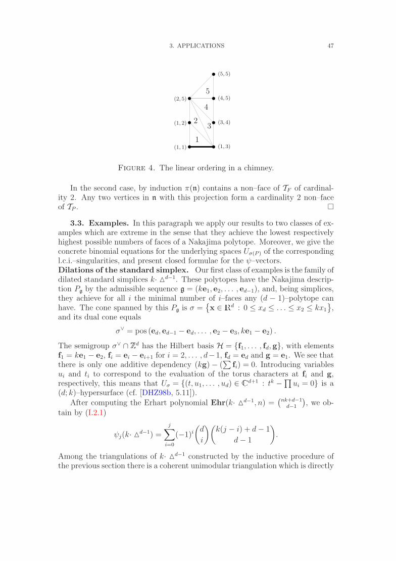
In the first case we stay within the chimney over π(n) ∈ TF . Thus, we mayassume that π(P ) = π(n). For all interior points x of π(P ) the linear orderingof the maximal simplices of TP by their intersections with the line π−1(x) is thesame, say, s1, . . . , sr. Assign to each lattice point m ∈ P ∩ Zd two numbers(m,M): M(m) = maxi : m ∈ si and m(m) = mini : m ∈ si, as illustratedin Figure 4 for a 2–dimensional Nakajima polytope.
Two vertices m,m′ belong to the same maximal simplex si of TP if and onlyif m(m),m(m′) ≤ i ≤ M(m),M(m′). Such an index i can be found if and onlyif m(m) ≤ M(m′) and m(m′) ≤ M(m). Furthermore, if m ∈ si ∩ sj, then alsom ∈ sk for all k between i and j.
Let n↑ ∈ n be a vertex with maximal m and n↓ ∈ n a vertex with minimal M .Since n is a non–face, we have m(n↑) > M(n↓). Hence n↑ and n↓ do not belongto a common maximal simplex, and n↓,n↑ ⊆ n is therefore a non–face of TP .
3. APPLICATIONS 47
(1, 2)
(2, 5)
(1, 1)
(5, 5)
(3, 4)
(1, 3)
(4, 5)
3
1
4
5
2
Figure 4. The linear ordering in a chimney.
In the second case, by induction π(n) contains a non–face of TF of cardinal-ity 2. Any two vertices in n with this projection form a cardinality 2 non–faceof TP .
3.3. Examples. In this paragraph we apply our results to two classes of ex-amples which are extreme in the sense that they achieve the lowest respectivelyhighest possible numbers of faces of a Nakajima polytope. Moreover, we give theconcrete binomial equations for the underlying spaces Uσ(P ) of the correspondingl.c.i.–singularities, and present closed formulae for the ψ–vectors.Dilations of the standard simplex. Our first class of examples is the family ofdilated standard simplices k· Md−1. These polytopes have the Nakajima descrip-tion Pg by the admissible sequence g = (ke1, e2, . . . , ed−1), and, being simplices,they achieve for all i the minimal number of i–faces any (d − 1)–polytope canhave. The cone spanned by this Pg is σ =
x ∈ Rd : 0 ≤ xd ≤ . . . ≤ x2 ≤ kx1
,
and its dual cone equals
σ∨ = pos (ed, ed−1 − ed, . . . , e2 − e3, ke1 − e2) .
The semigroup σ∨ ∩ Zd has the Hilbert basis H = f1, . . . , fd,g, with elementsf1 = ke1 − e2, fi = ei − ei+1 for i = 2, . . . , d−1, fd = ed and g = e1. We see thatthere is only one additive dependency (kg) − (
∑fi) = 0. Introducing variables
ui and ti to correspond to the evaluation of the torus characters at fi and g,respectively, this means that Uσ = (t, u1, . . . , ud) ∈ Cd+1 : tk −
∏ui = 0 is a
(d; k)–hypersurface (cf. [DHZ98b, 5.11]).After computing the Erhart polynomial Ehr(k· Md−1, n) =
(nk+d−1
d−1
), we ob-
tain by (I.2.1)
ψj(k· Md−1) =
j∑i=0
(−1)i
(d
i
)(k(j − i) + d − 1
d − 1
).
Among the triangulations of k· Md−1 constructed by the inductive procedure ofthe previous section there is a coherent unimodular triangulation which is directly
48 III. CREPANT RESOLUTIONS OF TORIC L.C.I.–SINGULARITIES
induced by an infinite hyperplane arrangement. The families of hyperplanes
Hi,j(k) = x ∈ Rd−1 : xi − xj = k (i, j ∈ Z) and
Hi(k) = x ∈ Rd−1 : xi = k (i ∈ Z)
form an arrangement H that triangulates the entire ambient space Rd−1 cohe-rently and unimodularly. Since the facets of k· Md−1 span hyperplanes of H, itis enough to consider the restriction T of this H–triangulation to k· Md−1. Theadvantage of this new triangulation is the uniform nature of its vertex stars.Choose a triangulation–vertex, which is not a vertex of k· Md−1, and translate itto the origin. Then the cones generated by the simplices that contain the givenvertex determine a fan defining an exceptional prime divisor of φT : XT → Uσ. Inparticular, the compactly supported exceptional prime divisors of φT correspondto the vertices lying in the interior of k· Md−1, and the star of each of them isnothing but the H–triangulation of a polytope which is lattice equivalent to thelattice zonotope
W (d−1) = conv([−1, 0]d−1 ∪ [0, 1]d−1
).
This shows that each compactly supported exceptional prime divisor of φT comesfrom the crepant full H–desingularization of a projective toric Fano variety, name-ly XN ((W (d−1))∨). The lattice points in (W (d−1))∨ are the origin together with thed(d − 1) points ±ei and ei − ej, for i 6= j. The corresponding points in thecone σ((W (d−1))∨) form a Hilbert basis, because (W (d−1))∨ admits a unimodularcover (even a triangulation). Hence the target space of the embedding described
in § I.4.2 is Pd(d−1). The degree of this embedding is(2(d−1)
d−1
), the normalized
volume of (W (d−1))∨: The intersection of (W (d−1))∨ with the cube [−1, 0]d− ×[0, 1]d+ (d−+d+ = d−1) is the product of a d− and a d+–dimensional unimodularsimplex that has the normalized volume
(d−1d−
). Coordinate permutations yield(
d−1d−
)such intersections. Adding up, we obtain
∑d−
(d−1d−
)(d−1d−
)=
(2(d−1)
d−1
).
Products of intervals. Our second class of examples is the family of hyper–intervals [0, a] = [0, a1]×· · ·× [0, ad] for integers ai > 0. These polytopes have theNakajima description Pg by the admissible sequence g = (a1e1, . . . , ade1) and forall i achieve the maximal number of i–faces any d–dimensional Nakajima polytopecan have. The cone spanned by this Pg is σ =
x ∈ Rd+1 : 0 ≤ xi ≤ aixd+1
,
σ∨ = pos (e1, . . . , ed, a1ed+1 − e1, . . . , aded+1 − ed) ,
and σ∨ ∩ Zd+1 is generated by H = f1, . . . , fd,g1, . . . ,gd,h with fi = ei
and gi = aied+1 − ei for i = 1, . . . , d, and h = ed+1. The d linear relations(fi + gi) − (aih) = 0 form a basis for the lattice of integral linear dependences ofH. Introducing one variable ui for each fi, vi for gi and t for h, these give rise tothe equations uivi − tai = 0.
3. APPLICATIONS 49
Using the multiplicative behavior of the Ehrhart polynomial for products ofpolytopes, one obtains the following formula for the ψ–vector:
ψj([0, a]) =
j∑i=0
(−1)j
(d + 1
j
) d∏ν=1
((j − i)aν + 1
).
Note that this example also admits the H–triangulation discussed before.
50 III. CREPANT RESOLUTIONS OF TORIC L.C.I.–SINGULARITIES
CHAPTER IV
Stringy Hodge numbers of hypersurfaces in toric varieties
1. Introduction
1.1. Hypersurfaces. The objects of study in this chapter are compacti-fied generic hypersurfaces in projective toric varieties. To define these, we startwith a lattice polytope P ⊂ Rd. Every lattice point m ∈ Zd can be identifiedwith a Laurent monomial tm = tm1
1 . . . tmdd , which is a regular function on the
d–dimensional algebraic torus T = (C∗)d. Consider the Ehr(P, 1)–dimensionalvector space L(P ) of C–linear combinations f =
∑m∈P∩Zd λmtm. The zero locus
Zf → T of such an f is a hypersurface in the torus. The projective toric varietyXP := XN (P ) contains T as an open and dense subset. The closure Zf in thecompactification XP of T is a compactified hypersurface. The data f , Zf andZf are called generic (or, more precisely P–regular) if for every face F ¹ P theintersection Zf ∩ TF with the (dim F )–dimensional torus corresponding to F iseither empty or a smooth hypersurface of TF . The name is justified by the factthat the set of Laurent polynomials f , for which Zf is generic, is open and densein L(P ) with respect to Zariski topology.
In the sequel we only write Z → XP and mean that the respective statementholds for every generic hypersurface. For a comprehensive treatment of theseobjects consult Batyrev [Bat94].
1.2. Hodge numbers. Let X be a compact smooth complex variety. Thenthere is a pure Hodge decomposition of its cohomology.
Hk(X,Q) ⊗C =⊕
p+q=k
Hp,q(X),
such that Hp,q(X) = Hq,p(X) (complex conjugation in C). The dimensions
hp,q(X) := dimCHp,q(X,C)
are called the (usual) Hodge numbers of X (cf. [GH94]). They are symmetric,hp,q = hq,p, they satisfy Serre duality hp,q = hdim X−p,dim X−q, and they vanish un-less 0 ≤ p, q ≤ dim X. For a general complex variety X Deligne [Del71, Del74]constructed a so–called mixed Hodge structure, giving rise to Hodge–Deligne num-bers hp,q(Hk(X,Q)), that agree with the usual ones in the smooth compact case:hp,q(Hk(X,Q)) = δk,p+qh
p,q(X). The same theory can be built on cohomologywith compact support H∗
c(X,Q), which is the right theory for our computations.
51
52 IV. STRINGY HODGE NUMBERS OF HYPERSURFACES IN TORIC VARIETIES
1.1. Definition (Danilov and Khovanskiı [DK87]). Define the E–polynomial ofa complex variety X by
ep,q(X) :=
2 dimCX∑k=0
(−1)khp,q(Hkc (X,Q)) ,
E(X; u, v) :=
dimCX∑p,q=0
ep,q(X)upvq .
Observe that in the smooth compact case ep,q(X) = (−1)p+qhp,q(X), so theHodge numbers can be read off from the E–polynomial. This polynomial has thefollowing nice properties.
1.2. Theorem [DK87].
• E(point; u, v) = 1 .
• E(X1 t X2; u, v) = E(X1; u, v) + E(X2; u, v)for disjoint locally closed subvarieties X1, X2 ⊂ X.
• E(X1 × X2; u, v) = E(X1; u, v) · E(X2; u, v). ¤
So E–polynomials should be easy to compute for nicely stratified varieties.
1.3. Corollary [DK87]. Let φ : X −→ X be a locally trivial fibering (inZariski topology) with fiber F . Then
E(X; u, v) = E(X; u, v) E(F ; u, v).
Proof. We use induction on the cardinality n of a trivializing open coverX =
⋃ni=1 Xi. For n = 1 the assertion is included in Theorem 1.2. For n > 1 de-
compose X = (X ′ r Xn) t (X ′ ∩ Xn) t (Xn r X ′) with X ′ =⋃n−1
i=1 Xi and applythe induction hypothesis to the restrictions of φ.
Theorem 1.2 enables us to calculate the first important E–polynomials.
1.4. Example. The projective line P1 is a smooth compact variety. As areal manifold it is a 2–sphere. The only non–trivial cohomology groups areH0(P1;Q) = H2(P1;Q) = Q. This already determines its Hodge numbers. Theyhave to be h0,0(P1) = h1,1(P1) = 1 and h0,1(P1) = h1,0(P1) = 0. So
E(P1; u, v) = uv + 1 ,E(C = P1 r ∞; u, v) = uv ,E(C∗ = P1 r 0,∞; u, v) = uv − 1 ,E((C∗)d; u, v) = (uv − 1)d .
¤
1. INTRODUCTION 53
A Calabi–Yau variety X is a normal compact variety with at most Gorensteincanonical singularities, KX = 0 and H1(X,OX) = . . . = Hdim X−1(X,OX) = 0.The mirror duality conjecture in theoretical physics suggests that every smoothd–dimensional Calabi–Yau variety X should have a family of “mirror partners”X, whose Hodge numbers satisfy
hp,q(X) = hdim X−p,q(X).(1.1)
Among the many references concerning the mathematical aspects of mirrorsymmetry we recommend [CK99, Mor97].
In many known mirror constructions, mirror partners have singularities. Inthis case the mirror symmetry identity (1.1) is expected to hold for crepant reso-lutions instead — if such exist. One could try to replace smooth crepant desingu-larizations by maximal crepant partial desingularizations. Although these alwaysexist, they are not unique and their cohomology groups and Hodge numbers arenot determined by the underlying spaces. The way out is to consider new Hodgenumbers hp,q
Str instead. They should satisfy three properties:
• hp,qStr(X) = hp,q(X) for smooth X,
• hp,q(X) = hp,qStr(X) for a crepant desingularization X −→ X,
• hp,qStr(X) = hd−p,q
Str (X).
Consider an affine Gorenstein toric variety Uσ(P ) that admits an invariant crepantdesingularization φ : XT → UP induced by a unimodular triangulation T of P .We should have hp,q
Str(Uσ(P )) = hp,q(XT ). So let us calculate the E–polynomialof XT .
1.5. Proposition (Batyrev and Dais [BD96]). Let φ : XT → Uσ(P ) be an in-variant crepant desingularization. Then
E(XT ; u, v) =∑F¹P
E(TF ; u, v)Ψ(F ; uv).(1.2)
Cf. I.2.3 for the Ψ–polynomial of a lattice polytope.
Proof. The stratification Uσ(P ) =⊔
F¹P TF into tori induces a stratification
of XT =⊔
F¹P φ−1(TF ). The stratum φ−1(TF ) is itself stratified by tori Ts ofdimension d − dim s corresponding to simplices s ∈ T with relint s ⊆ relint F .(Denote by fk(Trelint F ) the number of such k–simplices.) Then
E(φ−1(TF ); u, v) =dim F∑k=0
fk(Trelint F )(uv − 1)d−k.
54 IV. STRINGY HODGE NUMBERS OF HYPERSURFACES IN TORIC VARIETIES
On the other hand we can count lattice points in dilations of F by inclusion/ex-clusion
Ψ(F ; uv) = (1 − uv)dim F+1∑n≥0
Ehr(F, n)(uv)n
= (1 − uv)dim F+1∑n≥0
dim F∑k=0
(−1)dim F−kfk(Trelint F )
(n + k
k
)(uv)n
= (1 − uv)dim F+1
dim F∑k=0
(−1)dim F−kfk(Trelint F )1
(1 − uv)k+1
=dim F∑k=0
fk(Trelint F )(uv − 1)dim F−k.
Both expressions differ by a factor (uv − 1)d−dim F = E(TF ; u, v). Hence,
E(φ−1(TF ); u, v) = E(TF ; u, v)Ψ(F ; uv),
E(XT ; u, v) =∑F¹P
E(TF ; u, v)Ψ(F ; uv).
The restriction φ : φ−1(TF ) → TF is TF invariant. In general, given a group Gand a G–equivariant map φ : X ³ G onto G, the group operation (g, x) 7→ gx isan isomorphism G × φ−1(1G) → X. Thus φ−1(TF ) ∼= φ−1(point ∈ TF ) × TF , andwe recover Ψ(F ; uv) as the E–polynomial of any fiber φ−1(point).
The right hand side of (1.2) can also be computed if Uσ(P ) does not admitany crepant desingularization. This motivates the following definition.
1.6. Definition [BD96]. Let X =⊔
Xi be a stratified variety with Gorensteinsingularities such that (X,Xi) is locally isomorphic to (Cd×Uσ(Pi),C
d×0). Thenthe polynomial
EStr(X; u, v) =∑
ep,qStr(X)upvq :=
∑E(Xi; u, v)Ψ(Pi; uv)
is the string theoretic E–polynomial and the numbers hp,qStr(X) := (−1)p+qep,q
Str(X)are the string theoretic Hodge numbers.
Though up to now these are mere formally defined numbers, they have manyproperties which one could expect from cohomology dimensions. They are non–negative and symmetric, they satisfy Serre duality and also our three conditions.It is expected that there is some string theoretic cohomology theory that producesthese numbers [BB96, Remark 4.4]. Also, there already is a more or less concretecandidate, conjectured by Borisov [Bor, 9.23].
1. INTRODUCTION 55
Stringy Hodge numbers are preserved by (maximal) crepant partial desingu-larizations.
1.7. Theorem [BD96, Theorem 6.12]. Let X → X be a maximal crepant par-tial desingularization of a variety X with (at most) toroidal Gorenstein singular-
ities. Then hp,qStr(X) = hp,q
Str(X). ¤
If P is reflexive, then any generic hypersurface Z → XP is Calabi–Yau [Bat94,Theorem 4.1.9]. Good candidates for mirror partners are the generic hypersur-
faces Z∨
→ XP∨ .
1.8. Theorem [BB96, Theorem 4.15]. Any pair of compactified generic hyper-
surfaces Z → XP and Z∨
→ XP∨ satisfies the (stringy) mirror symmetry identity
hp,qStr(Z) = hd−p−1,q
Str (Z∨). ¤
1.3. Danilov–Khovanskiı formulae. In this paragraph we will outline theprincipal ideas of Danilov and Khovanskiı [DK87], who gave formulae for the usualHodge numbers of a generic hypersurface in a smooth projective toric variety interms of the corresponding lattice polytope.
As our toric varieties XP are stratified by tori — one (dimF )–dimensionaltorus for the (d − dim F )–dimensional normal cone corresponding to each faceF ¹ P — we have:
1.9. Proposition. Let P ⊂ Rd be a d–dimensional lattice polytope and XP
the associated projective toric variety. Then
E(XP ; u, v) =∑F¹P
(uv − 1)dim F , and thus
ep,q(XP ) = δp,q(−1)p
d∑k=p
(−1)kfk(P )
(k
p
).
For large p, q this result carries over to generic hypersurfaces Z → XP by thefollowing Lefschetz–type theorem.
1.10. Theorem [DK87]. Let P ⊂ Rd be a d–dimensional lattice polytope andZ → XP a compactified generic hypersurface in the associated projective toricvariety. If p + q > d − 1, then ep,q(Z) = ep+1,q+1(XP ). ¤
For the rest of the section we assume N (P ) to be unimodular. Then both Zand XP are smooth so that Poincare duality holds:
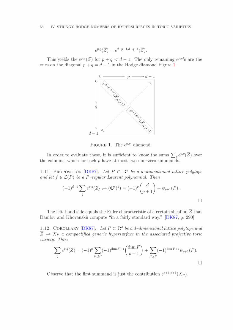
56 IV. STRINGY HODGE NUMBERS OF HYPERSURFACES IN TORIC VARIETIES
ep,q(Z) = ed−p−1,d−q−1(Z).
This yields the ep,q(Z) for p + q < d − 1. The only remaining ep,q’s are theones on the diagonal p + q = d − 1 in the Hodge diamond Figure 1.
e d−p,d−
p(XN
(P) )
e p+1,p+
1(XN
(P) )?
?
p
q
00 d − 1
d − 1
Figure 1. The ep,q–diamond.
In order to evaluate these, it is sufficient to know the sums∑
q ep,q(Z) overthe columns, which for each p have at most two non–zero summands.
1.11. Proposition [DK87]. Let P ⊂ Rd be a d–dimensional lattice polytopeand let f ∈ L(P ) be a P–regular Laurent polynomial. Then
(−1)d−1∑
q
ep,q(Zf → (C∗)d) = (−1)p
(d
p + 1
)+ ψp+1(P ).
¤
The left–hand side equals the Euler characteristic of a certain sheaf on Z thatDanilov and Khovanskiı compute “in a fairly standard way.” [DK87, p. 290]
1.12. Corollary [DK87]. Let P ⊂ Rd be a d–dimensional lattice polytope andZ → XP a compactified generic hypersurface in the associated projective toricvariety. Then∑
q
ep,q(Z) = (−1)p∑F¹P
(−1)dim F+1
(dim F
p + 1
)+
∑F¹P
(−1)dim F+1ψp+1(F ).
¤
Observe that the first summand is just the contribution ep+1,p+1(XP ).
1. INTRODUCTION 57
The following theorem reduces the computation of Hodge numbers to a purelycombinatorial task. It is the main tool for the calculation of string theoretic Hodgenumbers in the next section.
1.13. Theorem [DK87, § 5.5]. Let P be a d–polytope with unimodular normalfan, and let Z → XP be any generic compactified hypersurface. Then the Hodgenumbers hp,q(Z) vanish unless p = q or p + q = d − 1.For 2p > d − 1,
hp,p(Z) = (−1)p
d∑k=p+1
(−1)k+1
(k
p + 1
)fk(P ),
hp,d−p−1(Z) =∑F¹P
(−1)dim F+1ψp+1(F ).
For 2p = d − 1,
hp,p(Z) = (−1)p
d∑k=p+1
(−1)k+1
(k
p + 1
)fk(P ) +
∑F¹P
(−1)dim F+1ψp+1(F ).
For 2p < d − 1 the Hodge numbers may be obtained by duality:
hp,q(Z) = hd−p−1,d−q−1(Z).
¤
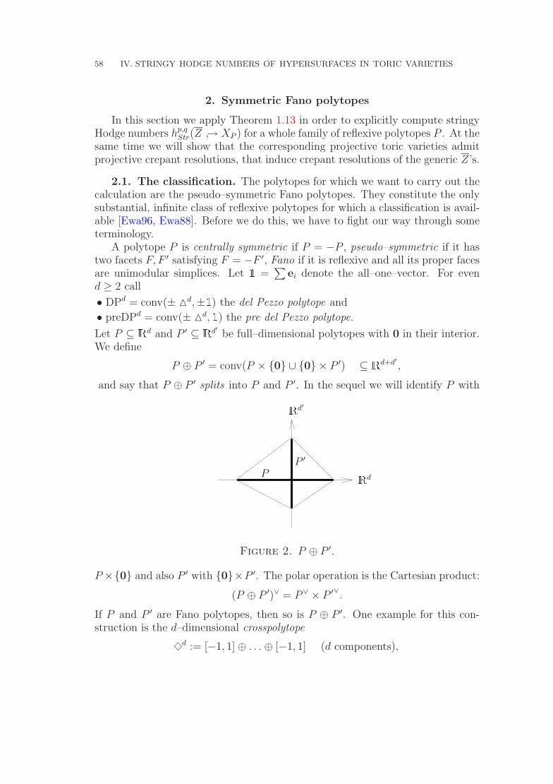
58 IV. STRINGY HODGE NUMBERS OF HYPERSURFACES IN TORIC VARIETIES
2. Symmetric Fano polytopes
In this section we apply Theorem 1.13 in order to explicitly compute stringyHodge numbers hp,q
Str(Z → XP ) for a whole family of reflexive polytopes P . At thesame time we will show that the corresponding projective toric varieties admitprojective crepant resolutions, that induce crepant resolutions of the generic Z’s.
2.1. The classification. The polytopes for which we want to carry out thecalculation are the pseudo–symmetric Fano polytopes. They constitute the onlysubstantial, infinite class of reflexive polytopes for which a classification is avail-able [Ewa96, Ewa88]. Before we do this, we have to fight our way through someterminology.
A polytope P is centrally symmetric if P = −P , pseudo–symmetric if it hastwo facets F, F ′ satisfying F = −F ′, Fano if it is reflexive and all its proper facesare unimodular simplices. Let 1 =
∑ei denote the all–one–vector. For even
d ≥ 2 call
• DPd = conv(± Md,±1) the del Pezzo polytope and
• preDPd = conv(± Md,1) the pre del Pezzo polytope.
Let P ⊆ Rd and P ′ ⊆ Rd′ be full–dimensional polytopes with 0 in their interior.We define
P ⊕ P ′ = conv(P × 0 ∪ 0 × P ′) ⊆ Rd+d′ ,
and say that P ⊕ P ′ splits into P and P ′. In the sequel we will identify P with
Rd
P ′
P
Rd′
Figure 2. P ⊕ P ′.
P ×0 and also P ′ with 0×P ′. The polar operation is the Cartesian product:
(P ⊕ P ′)∨ = P∨ × P ′∨.
If P and P ′ are Fano polytopes, then so is P ⊕ P ′. One example for this con-struction is the d–dimensional crosspolytope
¤d := [−1, 1] ⊕ . . . ⊕ [−1, 1] (d components),
2. SYMMETRIC FANO POLYTOPES 59
with its dual, the d–dimensional ±1–cube, ¤d := [−1, 1]d.Fight won; we can formulate:
2.1. Theorem [Ewa96, Ewa88]. Let P ⊆ Rd be a Fano polytope.
• If P is centrally symmetric, then it is equivalent to
¤d0 ⊕ DPd1 ⊕ . . . ⊕ DPdr .
• If P is pseudo–symmetric, then there is some centrally symmetric Fano poly-tope P ′, such that P is equivalent toP ′ ⊕ preDPd1 ⊕ . . . ⊕ preDPdr . ¤
We will achieve two things. We give give formulae for the hp,qStr of a generic
hypersurface within XP , when P is a pseudo–symmetric Fano polytope, andwe show that there is a crepant desingularization for them. Then our formulaecompute the usual Hodge numbers of these smooth varieties.
Our strategy for the first goal is to compute instead hd−p−1,qStr (Z
∨) of the mir-
ror (Z∨ → XP∨), because N (P∨), whose cones are spanned by the faces of P , isunimodular so that we can apply Theorem 1.13. The input that we need are theψ–vectors of all faces of P∨. So we have to analyze the components ((pre)DPd)∨
and [−1, 1] = [−1, 1]∨, i.e., identify their faces and compute the Ehrhart polyno-mials on the one hand and investigate the behavior of the input data with respectto Cartesian products on the other.
By the results of § III.1.2, the existence of crepant desingularizations boilsdown to the existence of a unimodular triangulation of N (P ) that is induced bytriangulations of the polytopes that span the σ ∈ N (P ), namely the faces of P∨.So, with both tasks we are left with questions about P∨.
2.2. The components. The triangulation part is an application of the upto now inappropriately unpublished Lemma 2.3, due to Francisco Santos (per-sonal communication (1997)). The counting part is based on a nice geometricinclusion/exclusion argument.Triangulations. The interval [−1, 1] admits the obvious coherent unimodulartriangulation, whose unique minimal non–face is the non–edge −1, 1. The factthat the polars of the (pre) del Pezzo’s also admit such triangulations is embed-ded into a more general context. Once more we use the refinement of a givensubdivision by pulling lattice points (cf. § I.2.2).
2.2. Definition. Let P be a lattice polytope and let 〈yi,x〉 ≥ ci be thefacet defining inequalities with primitive integral yi. Then P has facet widthmaxi widthyi
(P ). (Compare Section II.1 for the concept of width with respect toa given functional.)
In particular, P has facet width 1 if for every facet P lies between the hyper-plane spanned by this facet and the next parallel lattice hyperplane.
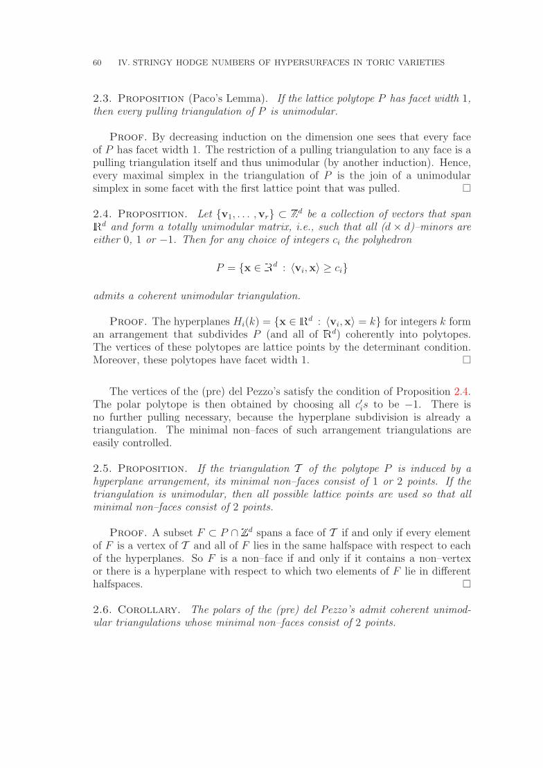
60 IV. STRINGY HODGE NUMBERS OF HYPERSURFACES IN TORIC VARIETIES
2.3. Proposition (Paco’s Lemma). If the lattice polytope P has facet width 1,then every pulling triangulation of P is unimodular.
Proof. By decreasing induction on the dimension one sees that every faceof P has facet width 1. The restriction of a pulling triangulation to any face is apulling triangulation itself and thus unimodular (by another induction). Hence,every maximal simplex in the triangulation of P is the join of a unimodularsimplex in some facet with the first lattice point that was pulled.
2.4. Proposition. Let v1, . . . ,vr ⊂ Zd be a collection of vectors that spanRd and form a totally unimodular matrix, i.e., such that all (d × d)–minors areeither 0, 1 or −1. Then for any choice of integers ci the polyhedron
P = x ∈ Rd : 〈vi,x〉 ≥ ci
admits a coherent unimodular triangulation.
Proof. The hyperplanes Hi(k) = x ∈ Rd : 〈vi,x〉 = k for integers k forman arrangement that subdivides P (and all of Rd) coherently into polytopes.The vertices of these polytopes are lattice points by the determinant condition.Moreover, these polytopes have facet width 1.
The vertices of the (pre) del Pezzo’s satisfy the condition of Proposition 2.4.The polar polytope is then obtained by choosing all c′is to be −1. There isno further pulling necessary, because the hyperplane subdivision is already atriangulation. The minimal non–faces of such arrangement triangulations areeasily controlled.
2.5. Proposition. If the triangulation T of the polytope P is induced by ahyperplane arrangement, its minimal non–faces consist of 1 or 2 points. If thetriangulation is unimodular, then all possible lattice points are used so that allminimal non–faces consist of 2 points.
Proof. A subset F ⊂ P ∩ Zd spans a face of T if and only if every elementof F is a vertex of T and all of F lies in the same halfspace with respect to eachof the hyperplanes. So F is a non–face if and only if it contains a non–vertexor there is a hyperplane with respect to which two elements of F lie in differenthalfspaces.
2.6. Corollary. The polars of the (pre) del Pezzo’s admit coherent unimod-ular triangulations whose minimal non–faces consist of 2 points.
2. SYMMETRIC FANO POLYTOPES 61
Ehrhart polynomials. As a warmup treat the interval [−1, 1]. The Ehrhartpolynomial is Ehr([−1, 1], k) = 2k + 1. Hence ψ0([−1, 1]) = ψ1([−1, 1]) = 1. Fitas we are now, we can endure some more notation. Denote by(
n
k1, . . . , kr
)=
n!
k1! · · · kr!, (k1 + . . . + kr = n),
the multinomial coefficient: the number of ordered partitions of an n–set into rsets of the respective sizes ki. In this notation, our familiar binomial coefficient(
nk
)is also denoted by
(n
k,n−k
)— so far the notational break.
The polar polytopes of the (pre) del Pezzos have the following description byinequalities:
(DPd)∨ = x ∈ [−1, +1]d :∑
xi ∈ [−1, +1] respectively
(preDPd)∨ = x ∈ [−1, +1]d−1 × (−∞, 1] :∑
xi ∈ [−1, +1].They are lattice equivalent to
x ∈ [−1, +1]d+1 :∑
xi = 0 respectively
x ∈ [−1, +1]d × (−∞, 1] :∑
xi = 0.(2.1)
The (pre) del Pezzos are simplicial, such that the ((pre)DPd)∨ are simplepolytopes (d is assumed to be even). This means that every (d − k)–face of thelatter is the intersection of k facets. Consider first the faces of (DPd)∨. The facetdefining inequalities in (2.1) are either of the form xi ≤ 1 or xi ≥ −1. A face Fsatisfies some of these inequalities with equality, say for i ∈ I+ ⊆ 1, . . . , d + 1the first one and for i ∈ I− the second one:
F = x ∈ [−1, +1]d+1 :∑
xi = 0, xi = 1(i ∈ I+), xi = −1(i ∈ I−).
We say that such a face is of type (d; s = card(I−), t = card(I+)). It has dimensiond′ = d − s − t and it is lattice equivalent to
F (d; s, t) = x ∈ [−1, +1]d′+1 :
∑xi = s − t.
If s, t ≤ d/2, then there are(
d+1d′+1,s,t
)such faces (otherwise F (d; s, t) is empty).
In the face poset of (preDPd)∨ there are other faces showing up. The facetdefining inequalities are the same as in the case of (DPd)∨, but the inequalityxd+1 ≥ −1 is missing. So, if d + 1 ∈ I+, the considered face is of type (d; s, t)and there are
(d
d′+1,s,t−1
)such faces, provided s, t ≤ d/2. But if the (d + 1)–st
coordinate is not fixed, we get a new kind of faces. They are equivalent to
F ′(d; s, t) = x ∈ [−1, +1]d′ × (−∞, 1] :
∑xi = s − t.
If s ≤ d/2, then there are(
dd′,s,t
)faces of that kind.
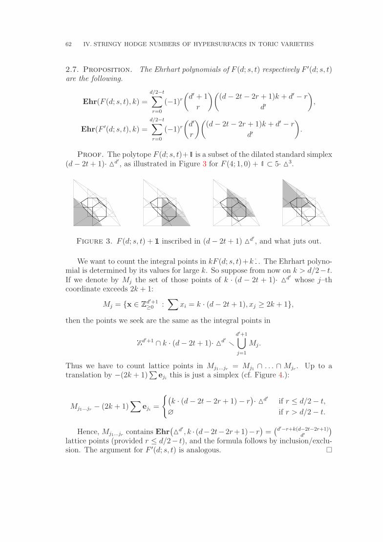
62 IV. STRINGY HODGE NUMBERS OF HYPERSURFACES IN TORIC VARIETIES
2.7. Proposition. The Ehrhart polynomials of F (d; s, t) respectively F ′(d; s, t)are the following.
Ehr(F (d; s, t), k) =
d/2−t∑r=0
(−1)r
(d′ + 1
r
)((d − 2t − 2r + 1)k + d′ − r
d′
),
Ehr(F ′(d; s, t), k) =
d/2−t∑r=0
(−1)r
(d′
r
)((d − 2t − 2r + 1)k + d′ − r
d′
).
Proof. The polytope F (d; s, t)+1 is a subset of the dilated standard simplex(d − 2t + 1)· Md′ , as illustrated in Figure 3 for F (4; 1, 0) + 1 ⊂ 5· M3.
Figure 3. F (d; s, t) + 1 inscribed in (d − 2t + 1) Md′ , and what juts out.
We want to count the integral points in kF (d; s, t)+k1. The Ehrhart polyno-mial is determined by its values for large k. So suppose from now on k > d/2− t.If we denote by Mj the set of those points of k · (d − 2t + 1)· Md′ whose j–thcoordinate exceeds 2k + 1:
Mj = x ∈ Zd′+1≥0 :
∑xi = k · (d − 2t + 1), xj ≥ 2k + 1,
then the points we seek are the same as the integral points in
Zd′+1 ∩ k · (d − 2t + 1)· Md′ rd′+1⋃j=1
Mj.
Thus we have to count lattice points in Mj1...jr = Mj1 ∩ . . . ∩ Mjr . Up to atranslation by −(2k + 1)
∑eji
this is just a simplex (cf. Figure 4.):
Mj1...jr − (2k + 1)∑
eji=
(k · (d − 2t − 2r + 1) − r
)· Md′ if r ≤ d/2 − t,
∅ if r > d/2 − t.
Hence, Mj1...jr contains Ehr(Md′ , k · (d−2t−2r +1)− r
)=
(d′−r+k(d−2t−2r+1)
d′)
lattice points (provided r ≤ d/2− t), and the formula follows by inclusion/exclu-sion. The argument for F ′(d; s, t) is analogous.
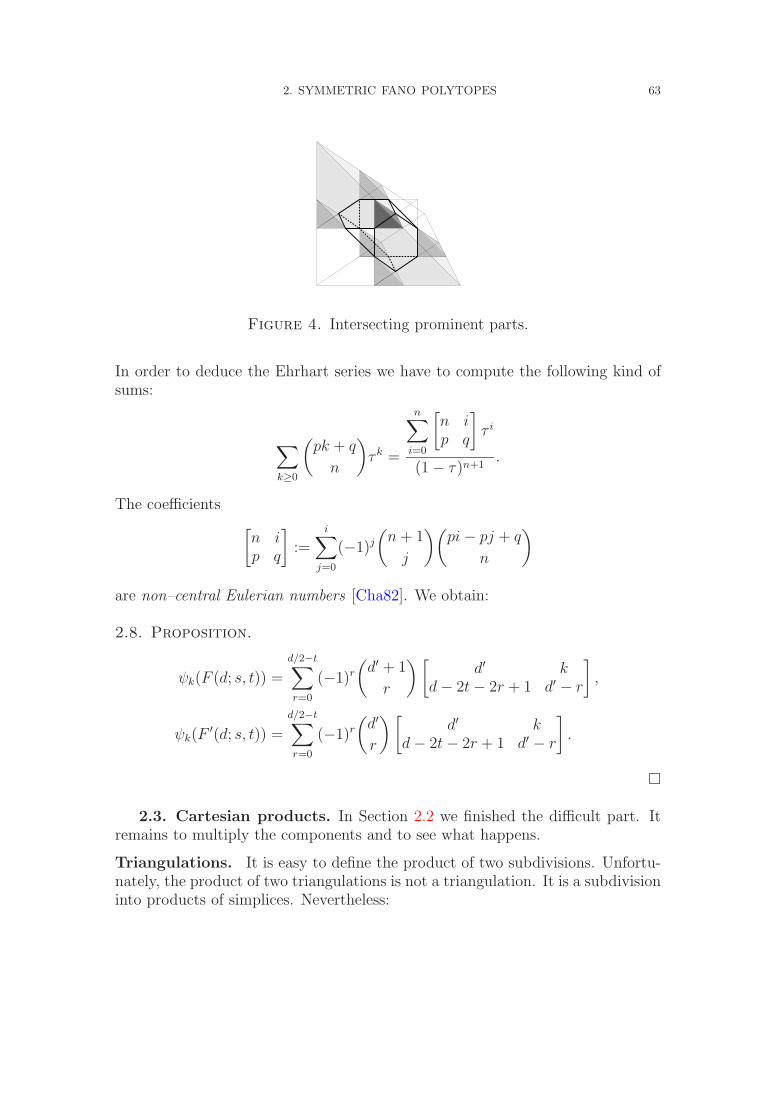
2. SYMMETRIC FANO POLYTOPES 63
Figure 4. Intersecting prominent parts.
In order to deduce the Ehrhart series we have to compute the following kind ofsums:
∑k≥0
(pk + q
n
)τ k =
n∑i=0
[n ip q
]τ i
(1 − τ)n+1.
The coefficients [n ip q
]:=
i∑j=0
(−1)j
(n + 1
j
)(pi − pj + q
n
)are non–central Eulerian numbers [Cha82]. We obtain:
2.8. Proposition.
ψk(F (d; s, t)) =
d/2−t∑r=0
(−1)r
(d′ + 1
r
)[d′ k
d − 2t − 2r + 1 d′ − r
],
ψk(F′(d; s, t)) =
d/2−t∑r=0
(−1)r
(d′
r
)[d′ k
d − 2t − 2r + 1 d′ − r
].
¤
2.3. Cartesian products. In Section 2.2 we finished the difficult part. Itremains to multiply the components and to see what happens.
Triangulations. It is easy to define the product of two subdivisions. Unfortu-nately, the product of two triangulations is not a triangulation. It is a subdivisioninto products of simplices. Nevertheless:
64 IV. STRINGY HODGE NUMBERS OF HYPERSURFACES IN TORIC VARIETIES
2.9. Proposition. Let P and P ′ be lattice polytopes. If both admit a (coherent)unimodular triangulation (whose minimal non–faces consist of 2 points), then sodoes P × P ′.
Proof. Any triangulation that refines the obvious (coherent) subdivisionof P × P ′ into products of unimodular simplices is unimodular, because anytriangulation of Md1 × Md2 is. See e.g. [Stu96, p.72, Ex.(9)] or [Lee97, p. 282].By the way, this product is a Nakajima polytope and it has facet width 1.
In order to preserve the non–face property, we have to be (a little) morecareful. Order the lattice points p1, . . . , pr in P and p′1, . . . , p′s in P ′. Then pullthe lattice points (pi, p
′j) in P × P ′ lexicographically.
Consider a non–face F . If one of its projections to P or P ′ is a non–face, we canlift a non–edge to F . Otherwise, F is a non–face in the staircase triangulationof a product of simplices (cf. [Lee97, p. 282]), i.e., there must be two points(p, p′), (q, q′) ∈ F that are not comparable in lexicographic order.
The Propositions 2.5 and 2.9 generalize a result of Bruns, Gubeladze andTrung [BGT97, Theorem 2.3.10]. Together they imply:
2.10. Corollary. Let P ⊂ Rd be a pseudo–symmetric Fano polytope. Thenits polar P∨ admits a coherent unimodular triangulation whose minimal non–facesconsist of 2 points. In particular, P∨ is Koszul. ¤
Retranslated into algebraic geometry this reads
2.11. Theorem. The toric Fano varieties XP associated with pseudo–sym-metric Fano polytopes P admit projective crepant resolutions. ¤
Ehrhart polynomials. The faces of P ×P ′ are the sets of the form F ×F ′ forfaces F, F ′ of P, P ′. Clearly
Ehr((F × F ′), n) = Ehr(F, n) · Ehr(F ′, n).
In order to calculate the ψ–vector of a general face
F = ¤d ×F (d1; s1, t1)×· · ·×F (dp; sp, tp)×F ′(d′1; s
′1, t
′1)×· · ·×F ′(d′
q; s′q, t
′q),
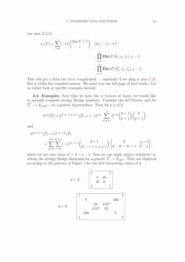
2. SYMMETRIC FANO POLYTOPES 65
one uses (I.2.1):
ψj(F ) =
j∑i=0
(−1)i
(dim F + 1
i
)(2(j − i) + 1)d
·p∏
ν=1
Ehr(F (dν ; sν , tν), j − i)
·q∏
µ=1
Ehr(F ′(d′µ; s′µ, t
′µ), j − i).
This will get a little bit (too) complicated — especially if we plug it into 1.13.But it yields the complete answer. We spare you one full page of bird tracks. Letus rather look at specific examples instead.
2.4. Examples. Now that we have the ψ–vectors at hand, we would liketo actually compute stringy Hodge numbers. Consider the del Pezzos, and let
Z∨
→ X(DPd)∨ be a generic hypersurface. Then for p ≥ d/2,
hp,p(Z) = hd−p−1,d−p−1(Z) = (−1)p+1
d∑k=p+1
2d−k
(d + 1
k + 1
)(k
p + 1
),
and
hp,d−p−1(Z) = hd−p−1,p(Z)
=
d/2∑s,t=0
d/2−t∑r=0
(−1)d′−r+1
(d + 1
d′ − r + 1, s, t, r
) [d′ p + 1
d − 2t − 2r + 1 d′ − r
],
where we set once more d′ = d − s − t. Now we can apply mirror symmetry toobtain the stringy Hodge diamonds for a generic Z → XDPd . They are depictedaccording to the pattern of Figure 1 for the first interesting values of d:
d = 4:
1 16 4646 6
1 1
d = 6:
1 18 386
29 41874187 29
386 81 1
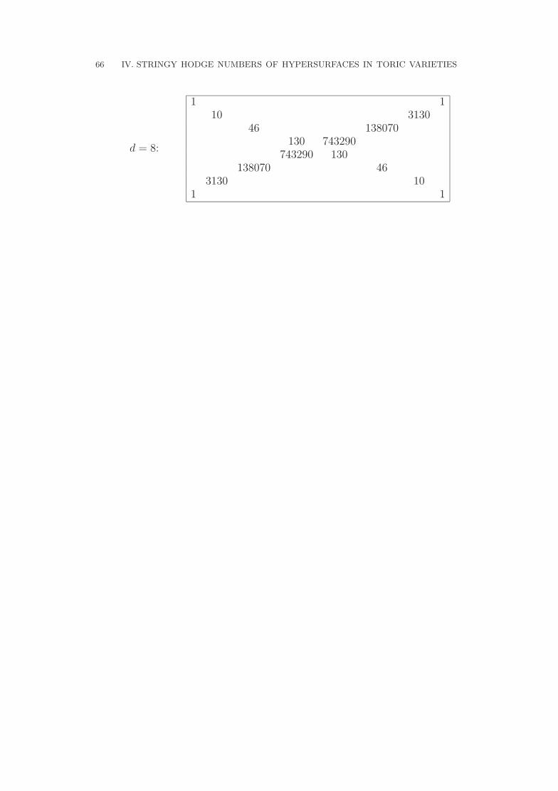
66 IV. STRINGY HODGE NUMBERS OF HYPERSURFACES IN TORIC VARIETIES
d = 8:
1 110 3130
46 138070130 743290
743290 130138070 46
3130 101 1
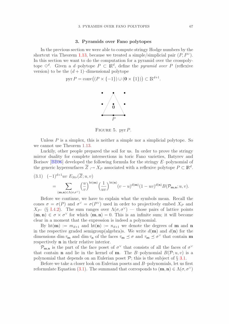
3. PYRAMIDS OVER FANO POLYTOPES 67
3. Pyramids over Fano polytopes
In the previous section we were able to compute stringy Hodge numbers by theshortcut via Theorem 1.13, because we treated a simple/simplicial pair (P, P∨).In this section we want to do the computation for a pyramid over the crosspoly-tope ¤d. Given a d–polytope P ⊂ Rd, define the pyramid over P (reflexiveversion) to be the (d + 1)–dimensional polytope
pyr P = conv((P × −1) ∪ (0 × 1)
)⊂ Rd+1.
P
0
Figure 5. pyr P .
Unless P is a simplex, this is neither a simple nor a simplicial polytope. Sowe cannot use Theorem 1.13.
Luckily, other people prepared the soil for us. In order to prove the stringymirror duality for complete intersections in toric Fano varieties, Batyrev andBorisov [BB96] developed the following formula for the stringy E–polynomial ofthe generic hypersurfaces Z → XP associated with a reflexive polytope P ⊂ Rd.
(3.1) (−1)d+1uv EStr(Z; u, v)
=∑
(m,n)∈Λ(σ,σ∨)
(u
v
)ht(m)( 1
uv
)ht(n)
(v − u)d(m)(1 − uv)d(n)B(Pm,n; u, v).
Before we continue, we have to explain what the symbols mean. Recall thecones σ = σ(P ) and σ∨ = σ(P∨) used in order to projectively embed XP andXP∨ (§ I.4.2). The sum ranges over Λ(σ, σ∨) — those pairs of lattice points(m,n) ∈ σ × σ∨ for which 〈m,n〉 = 0. This is an infinite sum; it will becomeclear in a moment that the expression is indeed a polynomial.
By ht(m) := md+1 and ht(n) := nd+1 we denote the degrees of m and nin the respective graded semigroup(algebra)s. We write d(m) and d(n) for thedimensions dim τm and dim τn of the faces τm ¹ σ and τm ¹ σ∨ that contain mrespectively n in their relative interior.
Pm,n is the part of the face poset of σ∨ that consists of all the faces of σ∨
that contain n and lie in the kernel of m. The B–polynomial B(P; u, v) is apolynomial that depends on an Eulerian poset P; this is the subject of § 3.1.
Before we take a closer look on Eulerian posets and B–polynomials, let us firstreformulate Equation (3.1). The summand that corresponds to (m,n) ∈ Λ(σ, σ∨)
68 IV. STRINGY HODGE NUMBERS OF HYPERSURFACES IN TORIC VARIETIES
only depends on the cones τm spanned by Fm ¹ P respectively τn spanned byFn ¹ P∨ on the one hand and on the heights m := ht(m) and n := ht(n) onthe other. In particular, the poset Pm,n is an interval in the face poset of σ∨;[τn, τ∨
m] := τ ¹ σ∨ : τn ¹ τ ¹ τ∨m. There are Ehr(Fm,m) lattice points with
height m in the relative interior of σm and Ehr(Fn, n) lattice points with heightn in the relative interior of σn.
(−1)d+1uv EStr(Z; u, v)
=∑
τm¹σ
(v − u)dim τm∑m≥0
Ehr(Fm,m)(u
v
)m
·∑
τn≺τ∨m
B([τn, τ∨m]; u, v)
· (1 − uv)dim τn∑n≥0
Ehr(Fn, n)
(1
uv
)n
.
(3.2)
The remaining infinite sums are inner Ehrhart series (cf. § I.2.3) so that we obtain
(−1)d+1uv EStr(Z; u, v)
=∑
Fm¹P
dim Fm+1∑j=1
ϕj(Fm)ujvdim Fm−j+1
·∑
Fn¹F∨m
B([Fn, F∨m]; u, v)
· (−1)dim Fn+1
dim Fn+1∑j=1
ϕj(Fn)(uv)dim Fn−j+1.
(3.3)
This is in fact a polynomial.
3.1. Eulerian posets. Let P be a finite poset with unique minimal ele-ment 0 and unique maximal element 1. An interval is a subposet of the form[p, p′] = q ∈ P : p ≤ q ≤ p′. We will use the shorthand [p, p] to denote theone point poset. Define recursively the Mobius function µ on such posets byµ[p, p] = 1 and
∑q∈[p,p′] µ[p, q] = 0 for p < p′. Call P graded if every maximal
chain has the same length rk(P). If P is graded then so is every interval. De-fine the rank function rk(p) to be the length of a maximal chain in [0, p]. Agraded poset P is Eulerian [Sta97, § 3.14] if for any pair p ≤ p′ in P we haveµ[p, p′] = (−1)rk(p′)−rk(p).
The face poset of a pointed polyhedral cone σ is an example of an Eulerianposet with minimum 0, maximum σ, and rank function rk(τ) = dim τ .
3. PYRAMIDS OVER FANO POLYTOPES 69
3.1. Definition. Let P be an Eulerian poset of rank r. Define recursivelypolynomials G(P; t) by
G(P; t) = 1 if r = 0,
deg G(P; t) < r/2 and∑p∈P
(t − 1)rk(p)G([p, 1]; t) ≡ 0 mod tdr/2e if r ≥ 1.
Use these polynomials to define the polynomial B(P; u, v) by
B(P; u, v) = 1 if r = 0,∑p∈P
B([0, p]; u, v)ur−rk(p)G([p, 1],v
u) = G(P; uv) if r ≥ 1.
One way of producing new posets from old ones is to take the Cartesianproduct with the component–wise partial order. If P and P ′ are Eulerian, thenso is P ×P ′. In the case of face posets, the product operation corresponds to thejoin of cones.
A map H that associates to every (isomorphism class of an) Eulerian posetP an element H(P) of a fixed ring (e.g. Z[t1 . . . tr]) is multiplicative if
H(P × P ′) = H(P)H(P ′)
for every pair of Eulerian posets. Observe that H[p, p] = 1 in an integral domain,unless H vanishes on all Eulerian posets.
3.2. Lemma. Given H,H1, H2, with multiplicative H, such that
H1[p, p] = 1, H2[p, p] = 1, and∑p∈P
H1[0, p]H2[p, 1] = H(P).
Then H1 is multiplicative if and only if H2 is.
Proof. Use induction on the pairs (rk(P), rk(P ′)). Suppose that H1 is mul-tiplicative, and use that intervals in product posets can be decomposed intoproducts [(p, q), (p′, q′)] = [p, p′] × [q, q′].
0 = H(P × P ′) − H(P)H(P ′)
=∑
(p,p′)∈P×P ′H1([0, p] × [0, p′])H2([p, 1] × [p′, 1]) − H1[0, p] H1[0, p
′] H2[p, 1] H2[p′, 1]
= H1([0, 0] × [0, 0])H2(P × P ′) − H1[0, 0] H1[0, 0] H2(P)H2(P ′)
= H2(P × P ′) − H2(P)H2(P ′).
The converse is shown the same way.
3.3. Corollary. The B–polynomial is multiplicative.
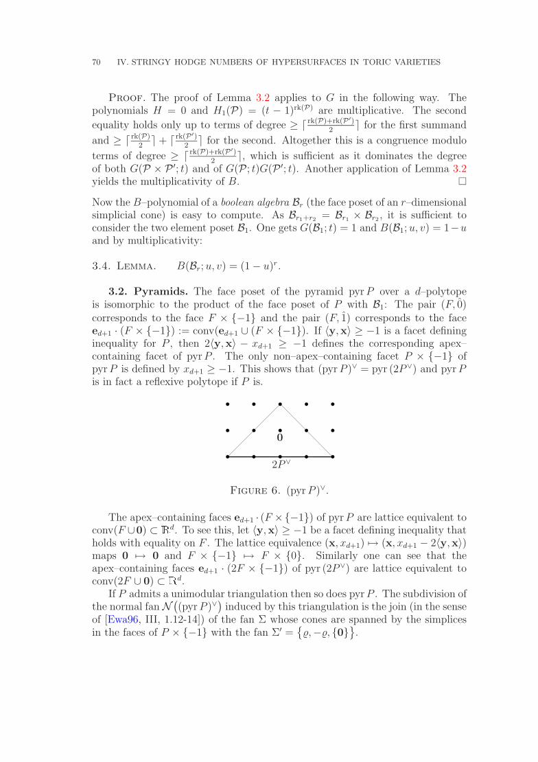
70 IV. STRINGY HODGE NUMBERS OF HYPERSURFACES IN TORIC VARIETIES
Proof. The proof of Lemma 3.2 applies to G in the following way. Thepolynomials H = 0 and H1(P) = (t − 1)rk(P) are multiplicative. The second
equality holds only up to terms of degree ≥ d rk(P)+rk(P ′)2
e for the first summand
and ≥ d rk(P)2
e + d rk(P ′)2
e for the second. Altogether this is a congruence modulo
terms of degree ≥ d rk(P)+rk(P ′)2
e, which is sufficient as it dominates the degreeof both G(P × P ′; t) and of G(P; t)G(P ′; t). Another application of Lemma 3.2yields the multiplicativity of B.
Now the B–polynomial of a boolean algebra Br (the face poset of an r–dimensionalsimplicial cone) is easy to compute. As Br1+r2 = Br1 × Br2 , it is sufficient toconsider the two element poset B1. One gets G(B1; t) = 1 and B(B1; u, v) = 1−uand by multiplicativity:
3.4. Lemma. B(Br; u, v) = (1 − u)r.
3.2. Pyramids. The face poset of the pyramid pyr P over a d–polytopeis isomorphic to the product of the face poset of P with B1: The pair (F, 0)corresponds to the face F × −1 and the pair (F, 1) corresponds to the faceed+1 · (F × −1) := conv(ed+1 ∪ (F × −1). If 〈y,x〉 ≥ −1 is a facet defininginequality for P , then 2〈y,x〉 − xd+1 ≥ −1 defines the corresponding apex–containing facet of pyrP . The only non–apex–containing facet P × −1 ofpyr P is defined by xd+1 ≥ −1. This shows that (pyrP )∨ = pyr (2P∨) and pyr Pis in fact a reflexive polytope if P is.
0
2P∨
Figure 6. (pyr P )∨.
The apex–containing faces ed+1 · (F ×−1) of pyr P are lattice equivalent toconv(F ∪0) ⊂ Rd. To see this, let 〈y,x〉 ≥ −1 be a facet defining inequality thatholds with equality on F . The lattice equivalence (x, xd+1) 7→ (x, xd+1 − 2〈y,x〉)maps 0 7→ 0 and F × −1 7→ F × 0. Similarly one can see that theapex–containing faces ed+1 · (2F × −1) of pyr (2P∨) are lattice equivalent toconv(2F ∪ 0) ⊂ Rd.
If P admits a unimodular triangulation then so does pyrP . The subdivision ofthe normal fan N
((pyr P )∨
)induced by this triangulation is the join (in the sense
of [Ewa96, III, 1.12-14]) of the fan Σ whose cones are spanned by the simplicesin the faces of P × −1 with the fan Σ′ =
%,−%, 0
.
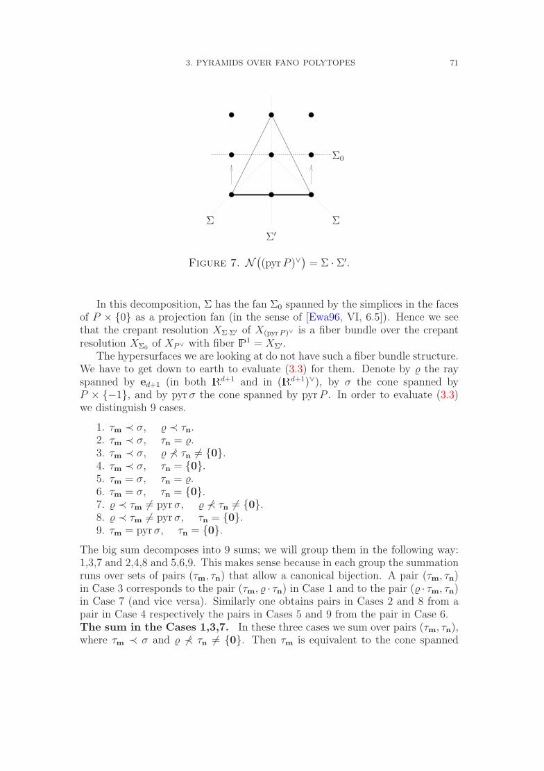
3. PYRAMIDS OVER FANO POLYTOPES 71
ΣΣ
Σ0
Σ′
Figure 7. N((pyr P )∨
)= Σ · Σ′.
In this decomposition, Σ has the fan Σ0 spanned by the simplices in the facesof P × 0 as a projection fan (in the sense of [Ewa96, VI, 6.5]). Hence we seethat the crepant resolution XΣ·Σ′ of X(pyr P )∨ is a fiber bundle over the crepantresolution XΣ0 of XP∨ with fiber P1 = XΣ′ .
The hypersurfaces we are looking at do not have such a fiber bundle structure.We have to get down to earth to evaluate (3.3) for them. Denote by % the rayspanned by ed+1 (in both Rd+1 and in (Rd+1)∨), by σ the cone spanned byP × −1, and by pyr σ the cone spanned by pyr P . In order to evaluate (3.3)we distinguish 9 cases.
1. τm ≺ σ, % ≺ τn.2. τm ≺ σ, τn = %.3. τm ≺ σ, % 6≺ τn 6= 0.4. τm ≺ σ, τn = 0.5. τm = σ, τn = %.6. τm = σ, τn = 0.7. % ≺ τm 6= pyr σ, % 6≺ τn 6= 0.8. % ≺ τm 6= pyr σ, τn = 0.9. τm = pyr σ, τn = 0.
The big sum decomposes into 9 sums; we will group them in the following way:1,3,7 and 2,4,8 and 5,6,9. This makes sense because in each group the summationruns over sets of pairs (τm, τn) that allow a canonical bijection. A pair (τm, τn)in Case 3 corresponds to the pair (τm, % · τn) in Case 1 and to the pair (% · τm, τn)in Case 7 (and vice versa). Similarly one obtains pairs in Cases 2 and 8 from apair in Case 4 respectively the pairs in Cases 5 and 9 from the pair in Case 6.The sum in the Cases 1,3,7. In these three cases we sum over pairs (τm, τn),where τm ≺ σ and % 6≺ τn 6= 0. Then τm is equivalent to the cone spanned
72 IV. STRINGY HODGE NUMBERS OF HYPERSURFACES IN TORIC VARIETIES
by some face Fm ≺ P , and τn is equivalent to the cone spanned by some face∅ 6= Fn ¹ F∨
m ¹ P∨, where duality takes place in Rd.In Case 1 we then have to evaluate the summand for the pair (Fm, ed+1 ·Fn),
in Case 3 for (Fm, Fn), and in Case 7 for (ed+1 · Fm, Fn). Each summand is aproduct of three factors. We investigate how they are affected when ed+1 is joinedto Fm respectively to Fn.
•∑dim Fm+1
j=1 ϕj(Fm)ujvdim Fm−j+1:
The cone % · τm is spanned by (a polytope that is lattice equivalent to) 0 · Fm.
There are Ehr(0 · Fm, k) =∑k−1
j=1 Ehr(Fm, j) lattice points interior to thedilations of this polytope. This affects the ϕ–vector as follows.
∑k≥1
k−1∑j=1
Ehr(F, j)tk =∑j≥1
Ehr(F, j)∑
k≥j+1
tk
=∑j≥1
Ehr(F, j)tj+1
1 − t
=t
1 − t
∑j≥1
Ehr(F, j)tj.
Hence we get a factor u:
dim Fm+2∑j=1
ϕj(ed+1 · Fm)ujvdim Fm−j+2 = u
dim Fm∑j=1
ϕj(Fm)ujvdim Fm−j+1.
• B([τn, τ∨m]; u, v):
% is a face of τm if and only if % on the dual side is not a face of τ∨m. Joining %
to τm corresponds under the above identification of face posets to descendingfrom the pair (F∨
m, 1) to (F∨m, 0). In a similar way, joining % to τn corresponds
to ascending from (Fn, 0) to (Fn, 1). We have the following isomorphisms.
[τn, τ∨m] ∼= B1 × [τn, (% · τm)∨] ∼= B1 × [% · τn, τ∨
m] ∼= B1 × [Fn, F∨m],
where F∨m is once more the face of P∨ dual to Fm. This yields the identities
B([τn, τ∨m]; u, v) = (1 − u)B([τn, (% · τm)∨]; u, v)
= (1 − u)B([% · τn, τ∨m]; u, v)
= (1 − u)B([Fn, F∨m]; u, v).
• (−1)dim Fn+1∑dim Fn+1
j=1 ϕj(Fn)(uv)dim Fn−j+1:For the moment we cannot say anything about this factor but that the signchanges if the dimension of τn rises by 1.
3. PYRAMIDS OVER FANO POLYTOPES 73
Altogether the contribution of the Cases 1,3,7 is∑Fm≺P
∑∅6=Fn¹F∨
m
dim Fm+1∑j=1
ϕj(Fm)ujvdim Fm−j+1(−1)dim Fn+1B([Fn, F∨m]; u, v)
(−
dim Fn+2∑j=1
ϕj(0 · (2Fn))(uv)dim Fn+2−j
+ (1 − u)dim Fn+1∑
j=1
ϕj(Fn)(uv)dim Fn−j+1
+ udim Fn∑
j=1
ϕj(Fn)(uv)dim Fn−j+1
)
=∑
Fm≺P
∑∅6=Fn¹F∨
m
dim Fm+1∑j=1
ϕj(Fm)ujvdim Fm−j+1(−1)dim Fn+1B([Fn, F∨m]; u, v)
·dim Fn+1∑
j=0
(ϕj(Fn) − ϕj+1(0 · (2Fn))
)(uv)dim Fn−j+1.
The sum in the Cases 2,4,8. In these three cases we only sum over τm ≺ σrespectively Fm ≺ P , and take τn = 0 respectively Fn = ∅.
In Case 2 we then have to evaluate the summand for the pair (Fm, ed+1),in Case 4 for (Fm, ∅), and in Case 8 for (0 · Fm, ∅).
•∑dim Fm+1
j=1 ϕj(Fm)ujvdim Fm−j+1:As before joining τm with % gives a factor u.
• B([τn, τ∨m]; u, v):
B([Fn, F∨m]; u, v) in Cases 2 and 8, (1 − u)B([Fn, F∨
m]; u, v) in Case 4.
• (−1)dim Fn+1∑dim Fn+1
j=1 ϕj(Fn)(uv)dim Fn−j+1:Easy: 1 in Cases 4 and 8, −1 in Case 2.
So this contribution is no contribution.
∑Fm≺P
dim Fm+1∑j=1
ϕj(Fm)ujvdim Fm−j+1B([∅, F∨m]; u, v)
(−1 + (1 − u) + u
)= 0.
The sum in the Cases 5,6,9. These three cases contain one pair each;(P, ed+1) in Case 5, (P, ∅) in Case 6, and (pyrP, ∅) in Case 9.
•∑dim Fm+1
j=1 ϕj(Fm)ujvdim Fm−j+1:This time we have to count in pyrP . The intersection of k pyr P with thehyperplane xd+1 = j for j ∈ [−k + 1, k − 1] is equivalent to k−j
2P . Thus,
if k − j = 2i is even, then there are Ehr(P, i) interior lattice points, and, if
74 IV. STRINGY HODGE NUMBERS OF HYPERSURFACES IN TORIC VARIETIES
k − j = 2i − 1 is odd, then there are Ehr(P, i) of them (recall that there areno lattice points between iP and (i + 1)P ).
Ehr(pyr P, k) =k∑
i=1
Ehr(P, i) +k−1∑i=1
Ehr(P, i).
We can once more exchange the summation.
∑k≥1
(k∑
i=1
Ehr(P, i) +k−1∑i=1
Ehr(P, i)
)tk =
∑i≥1
Ehr(P, i)
(tj
1 − t+
tj+1
1 − t
)=
1 + t
1 − t
∑i≥1
Ehr(P, i)ti.
Thus we get a factor of v + u in Case 9.
• B([τn, τ∨m]; u, v):
Easy: 1 in Cases 5 and 9, 1 − u in Case 6.
• (−1)dim Fn+1∑dim Fn+1
j=1 ϕj(Fn)(uv)dim Fn−j+1:Once more 1 in Cases 6 and 9, −1 in Case 5.
So there is a contribution
d+1∑j=1
ϕj(P )ujvd+1−j(−1 + (1 − u) + (u + v)
)=
d+1∑j=1
ϕj(P )ujvd+2−j.
Let us summarize what we have got.
3.5. Theorem. Let P ⊂ Rd be a reflexive d–polytope. The stringy E–poly-nomial EStr(Z; u, v) of a generic hypersurface Z → Xpyr P equals the followingexpression.
(−1)d
uv
(d+1∑j=1
ϕj(P )ujvd+2−j
+∑
Fm≺P
∑∅6=Fn¹F∨
m
dim Fm+1∑j=1
ϕj(Fm)ujvdim Fm−j+1(−1)dim Fn+1B([Fn, F∨m]; u, v)
·dim Fn+1∑
j=0
(ϕj(Fn) − ϕj+1(0 · 2Fn)
)(uv)dim Fn−j+1
).
3. PYRAMIDS OVER FANO POLYTOPES 75
3.6. Corollary. Let P ⊂ Rd be a d–dimensional Fano polytope. The stringyHodge numbers hp,q
Str(Z → Xpyr P ) of a generic hypersurface vanish unless p = qor p + q = d. In the latter cases they are given by
hp,pStr(Z) = (−1)d+1
∑∅6=F¹P∨
(−1)dim F(ψp+1(2F ) − ψp+1(0 · 2F )
),
hp,d−pStr (Z) = ϕp+1(P ),
if 2p 6= d. If 2p = d then one has
hp,pStr(Z) = ϕp+1(P ) + (−1)d+1
∑∅6=F¹P∨
(−1)dim F(ψp+1(2F ) − ψp+1(0 · 2F )
).
Proof. If P is Fano, then all its proper faces are unimodular, with the effectthat ϕj(Fm) = δj,dim Fm+1 and all intervals [Fn, F∨
m] with Fn 6= ∅ are boolean, withthe effect that B([Fn, F∨
m]; u, v) = (1 − u)d−dim Fm−dim Fn−1. Exchange the summa-tion to obtain
(−1)d
uv
(d+1∑j=1
ϕj(P )ujvd+2−j
+∑
∅6=Fn¹P∨(−1)dim Fn+1
dim Fn+1∑j=0
(ϕj(2Fn) − ϕj+1(0 · 2Fn)
)(uv)dim Fn−j+1
·∑
Fm¹F∨n
udim Fm+1(1 − u)d−dim Fm−dim Fn−1
).
The summands of the last sum only depend on dim Fm. Because Fn 6= ∅, F∨n is
a simplex, which has(
d−dim Fn
d′+1
)d′–faces. So this last sum evaluates to
d−dim Fn−1∑d′=−1
(d − dim Fn
d′ + 1
)ud′+1(1 − u)d−dim Fn−d′−1 = 1.
It remains to extract the coefficients of (uv)p and of upvd−p. Use the fact thatϕdim Fn−p(2Fn) = ψp+1(2Fn) and ϕdim Fn−p+1(0 · 2Fn) = ψp+1(0 · 2Fn).
If P = ¤d is the crosspolytope, then two faces of P∨ of the same dimensionare equivalent. Furthermore they are reflexive themselves so that we can computethe expression ψp+1(2F ) − ψp+1(0 · 2F ) as follows.
Ehr(0 · 2F, k) =2k∑
j=0
Ehr(F, j).
76 IV. STRINGY HODGE NUMBERS OF HYPERSURFACES IN TORIC VARIETIES
It is slightly more subtle to exchange the summation.
Ψ(0 · 2F ; t) =∑k≥0
2k∑j=0
Ehr(F, j)tk =∑j≥0
Ehr(F, j)∑
k≥d j2e
tk
=1
1 − t
(∑i≥0
Ehr(F, 2i)ti +∑i≥1
Ehr(F, 2i − 1)ti
)
=1
1 − t
(Ψ(2F ; t) +
∑i≥1
Ehr(F, 2i)ti
)
=1
1 − t
(Ψ(2F ; t) + Φ(2F ; t)
),
where we used Ehr(F, 2i − 1) = Ehr(F, 2i). It follows that
ψp+1(2F ) − ψp+1(0 · 2F ) = −ϕp+1(2F ).
3.7. Corollary. Let Z → Xpyr ¤d be a generic hypersurface. Then
hp,pStr(Z) =
d∑d′=p
(−1)d−d′(
d
d′
)2d−d′ϕp+1(2¤d′),
hp,d−pStr (Z) =
(d
p
),
if 2p 6= d. If 2p = d, then
hp,pStr(Z) =
(d
p
)+
d∑d′=p
(−1)d−d′(
d
d′
)2d−d′ϕp+1(2¤d′).
Proof. After the above considerations, all we have to do is to convince our-selves that
ϕp+1( ¤d) =
(d
p
).
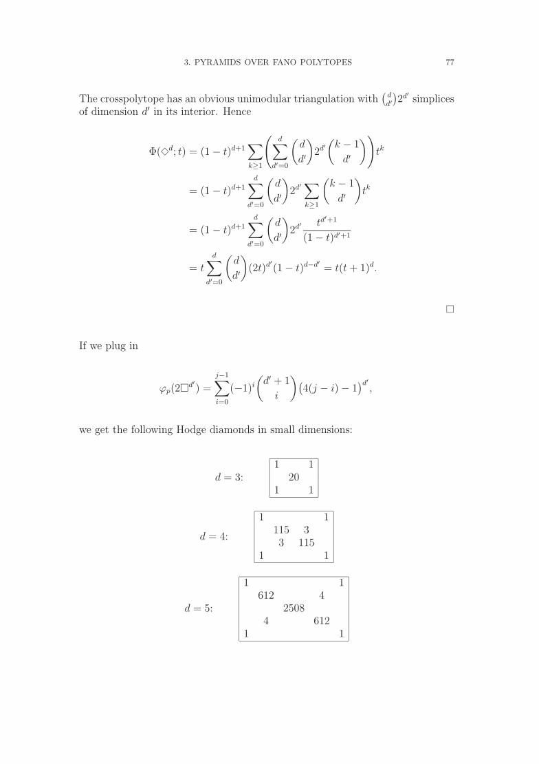
3. PYRAMIDS OVER FANO POLYTOPES 77
The crosspolytope has an obvious unimodular triangulation with(
dd′)2d′ simplices
of dimension d′ in its interior. Hence
Φ( ¤d; t) = (1 − t)d+1∑k≥1
(d∑
d′=0
(d
d′
)2d′
(k − 1
d′
))tk
= (1 − t)d+1
d∑d′=0
(d
d′
)2d′
∑k≥1
(k − 1
d′
)tk
= (1 − t)d+1
d∑d′=0
(d
d′
)2d′ td
′+1
(1 − t)d′+1
= t
d∑d′=0
(d
d′
)(2t)d′(1 − t)d−d′ = t(t + 1)d.
If we plug in
ϕp(2¤d′) =
j−1∑i=0
(−1)i
(d′ + 1
i
)(4(j − i) − 1
)d′,
we get the following Hodge diamonds in small dimensions:
d = 3:1 1
201 1
d = 4:
1 1115 33 115
1 1
d = 5:
1 1612 4
25084 612
1 1
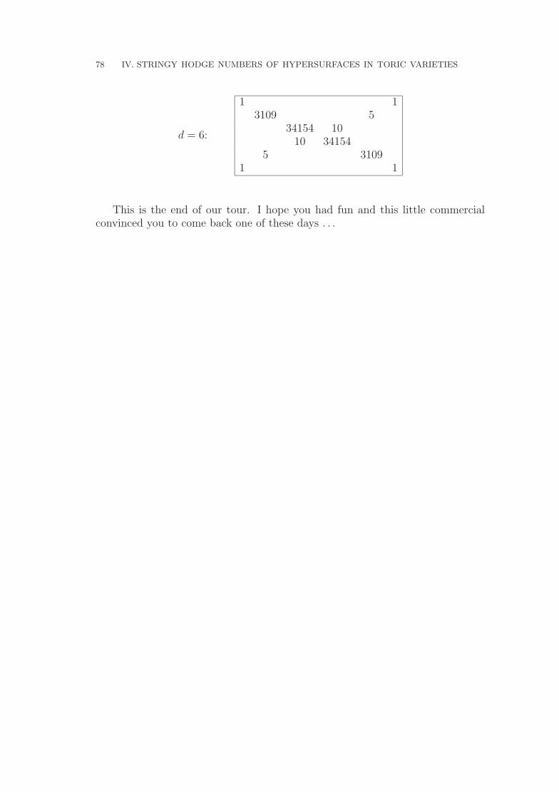
78 IV. STRINGY HODGE NUMBERS OF HYPERSURFACES IN TORIC VARIETIES
d = 6:
1 13109 5
34154 1010 34154
5 31091 1
This is the end of our tour. I hope you had fun and this little commercialconvinced you to come back one of these days . . .
Bibliography
[Bar94] Alexander I. Barvinok. A polynomial time algorithm for counting integral pointsin polyhedra when the dimension is fixed. Math. Oper. Res., 19:769–779, 1994.
[Bat94] Victor V. Batyrev. Dual polyhedra and mirror symmetry for Calabi–Yau hyper-surfaces in toric varieties. J. Alg. Geom., 3:493–535, 1994.
[Bat99] Victor V. Batyrev. Non–Archimedian integrals and stringy Euler numbers of log–terminal pairs. J. European Math. Soc., 1:5–33, 1999.
[BB96] Victor V. Batyrev and Lev A. Borisov. Mirror duality and string–theoretic Hodgenumbers. Inventiones Math., 126:183–203, 1996.
[BD96] Victor V. Batyrev and Dimitrios I. Dais. Strong McKay correspondence, string–theoretic Hodge numbers and mirror symmetry. Topology, 35:901–929, 1996.
[BG99] Winfried Bruns and Joseph Gubeladze. Normality and covering properties of affinesemigroups. J. Reine Angew. Math., 510:161–178, 1999.
[BGH+99] Winfried Bruns, Joseph Gubeladze, Martin Henk, Alexander Martin, and RobertWeismantel. A counterexample to an integer analogue of caratheodory’s theorem.J. Reine Angew. Math., 510:179–185, 1999.
[BGT97] Winfried Bruns, Joseph Gubeladze, and Ngo Viet Trung. Normal polytopes, tri-angulations and Koszul algebras. J. Reine Angew. Math., 485:123–160, 1997.
[BLPS98] Wojciech Banaszczyk, Alexander E. Litvak, Alain Pajor, and StanisÃlaw J. Szarek.The flatness theorem for non–symmetric convex bodies via the local theory ofBanach spaces. Preprint, 1998.
[Bor] Lev A. Borisov. Vertex algebras and mirror symmetry. LANL preprint alg–geom/9809094.
[BP98] Alexander I. Barvinok and James E. Pommersheim. An algorithmic theory oflattice points in polyhedra. Preprint, March 26 1998.
[Cha82] Charalambos A. Charalambides. On the enumeration of certain compositions andrelated sequences of numbers. Fibonacci Q., 20:132–146, 1982.
[CK99] David A. Cox and Sheldon Katz. Mirror Symmetry and Algebraic Geometry, vol-ume 68 of Math. Surveys and Monographs. AMS, 1999.
[Del71] Pierre Deligne. Theorie de Hodge II. Inst. Hautes Etudes Sci. Publ. Math., 40:5–57, 1971.
[Del74] Pierre Deligne. Theorie de Hodge III. Inst. Hautes Etudes Sci. Publ. Math., 44:5–77, 1974.
[DHa] Dimitrios I. Dais and Christian Haase. Stringy Hodge numbers of hypersurfacesin toric Fano varieties. In preparation.
[DHb] Dimitrios I. Dais and Martin Henk. On a series of Gorenstein cyclic quo-tient singularities admitting a unique projective crepant resolution. In G.Ewaldand B.Teissier, editors, Combinatorial Convex Geometry and Toric Varieties.Birkhauser. In print.
79
80 BIBLIOGRAPHY
[DHH98] Dimitrios I. Dais, Utz-Uwe Haus, and Martin Henk. On crepant resolutions of2–parameter series of Gorenstein cyclic quotient singularities. Results in Math.,33:208–265, 1998.
[DHZ98a] Dimitrios I. Dais, Christian Haase, and Gunter M. Ziegler. All toric l.c.i.-singularities admit projective crepant resolutions (long version). Technical Report614/1998, TU–Berlin, 1998.
[DHZ98b] Dimitrios I. Dais, Martin Henk, and Gunter M. Ziegler. All abelian quotient c.i.–singularities admit projective crepant resolutions in all dimensions. Advances inMath., 139:192–239, 1998.
[DHZ00] Dimitrios I. Dais, Christian Haase, and Gunter M. Ziegler. All toric l.c.i.-singularities admit projective crepant resolutions. Tohoku Math. J., to appear2000.
[DK87] V. I. Danilov and Askol’d G. Khovanskiı. Newton polyhedra and an algorithm forcomputing Hodge–Deligne numbers. Math. USSR Izvestiya, 29(2):279–298, 1987.
[Ehr77] Eugene Ehrhart. Polynomes arithmetiques et methode des polyedres en combina-toire, volume 35 of Int. ser. numerical math. Birkhauser, 1977.
[Ewa88] Gunter Ewald. On the classification of toric Fano varieties. Disc. Comp. Geom.,3:49–54, 1988.
[Ewa96] Gunter Ewald. Combinatorial Convexity and Algebraic Geometry, volume 168 ofGTM. Springer–Verlag, 1996.
[Ful93] William Fulton. Introduction to Toric Varieties, volume 131 of Annals of Math.Studies. Princeton University Press, 1993.
[FZ99] Robert T. Firla and Gunter M. Ziegler. Hilbert bases, unimodular triangulations,and binary coverings of rational polyhedral cones. Disc. Comp. Geom., 21:205–216, 1999.
[GH94] Phillip Griffiths and Joseph Harris. Principles of Algebraic Geometry. Wiley clas-sics library. John Wiley & Sons Ltd., 2nd edition, 1994.
[GK] Richtlinien fur Stipendiaten; Graduiertenkolleg ‘Algorithmische Diskrete Mathe-matik’. http://www.inf.fu-berlin.de/graduate-programs/adm/richtlinien.ps.gz.
[Hib92] Takayuki Hibi. Dual polytopes of rational convex polytopes. Combinatorica,12(2):237–240, 1992.
[HZ00] Christian Haase and Gunter M. Ziegler. On the maximal width of empty latticesimplices. Europ. J. Comb., 21:111–119, 2000.
[IR94] Yukari Ito and Miles Reid. The McKay correspondence for finite subgroups ofSL(3, C). In Marco Andreatta and Thomas Peternell, editors, Higher Dimen-sional Complex Varieties, Proc. Int. Conf. Trento, Italy, pages 221–240. de Gruyter(1996), June 1994.
[Khi48] A. Ja. Khinchine. Die quantitative Konzeption der Kroneckerschen Approxi-mationstheorie. (Russian). Izv. Akad. Nauk SSSR, Ser. Mat., 12:113–122, 1948.
[KKMSD73] George R. Kempf, Finn F. Knudsen, David Mumford, and Bernard Saint-Donat.Toroidal Embeddings I, volume 339 of Lecture Notes in Mathematics. Springer–Verlag, 1973.
[Lee97] Carl W. Lee. Subdivisions and triangulations of polytopes. In Jacob E. Goodmanand Joseph O’Rourke, editors, Handbook of Discrete and Computational Geome-try, pages 271–290. CRC–Press, New York, 1997.
[Len83] Hendrik W. Lenstra. Integer programming with a fixed number of variables. Math.Oper. Res., 8:538–548, 1983.
[Mor97] David R. Morrison. Mathematical aspects of mirror symmetry. In Janos Kollar,editor, Complex Algebraic Geometry, volume 3 of IAS/Park City Math. Ser., pages265–340. AMS, 1997.
BIBLIOGRAPHY 81
[MS84] David R. Morrison and Glenn Stevens. Terminal quotient singularities in dimen-sion 3 and 4. Proc. A.M.S., 90:15–20, 1984.
[Nak86] Haruhisa Nakajima. Affine torus embeddings which are complete intersections.Tohoku Math. J., 38:85–98, 1986.
[Oda88] Tadao Oda. Convex Bodies and Algebraic Geometry. An Introduction to the The-ory of Toric Varieties, volume 15 of Ergebnisse der Mathematik und ihrer Gren-zgebiete. Springer–Verlag, 1988.
[Ree57] John E. Reeve. On the volume of lattice polyhedra. Proc. London Math. Soc.,7:378–395, 1957.
[Rei] Miles Reid. McKay correspondence. preprint alg–geom/9702016.[Rei87] Miles Reid. Young person’s guide to canonical singularities. In Spencer J. Bloch,
editor, Algebraic Geometry, Bowdoin 1985, volume 46 of Proc. Symp. Pure Math.,pages 345–414. A.M.S., 1987.
[Sca85] Herbert E. Scarf. Integral polyhedra in three space. Math. Oper. Res., 10:403–438,1985.
[Seb90] Andras Sebo. Hilbert bases, Caratheodory’s theorem and combinatorial optimiza-tion. In Ravindran Kannan and William R. Pulleyblank, editors, Integer Program-ming and Combinatorial Optimization, pages 431–456. Math. Prog. Soc., Univ.Waterloo Press, 1990.
[Seb98] Andras Sebo. An introduction to empty lattice–simplices. Preprint, November1998.
[Ser56] Jean-Pierre Serre. Geometrie algebrique et geometrie analytique. Ann. Inst.Fourier, 6:1–42, 1956.
[Sta97] Richard P. Stanley. Enumerative Combinatorics, volume I. Cambridge UniversityPress, 2nd edition, 1997.
[Stu96] Bernd Sturmfels. Grobner Bases and Convex Polytopes, volume 8 of UniversityLecture Series. A.M.S., 1996.
[Wah99] Elias Wahidi. Berechnung der Weite und Aquivalenz elementarer Gittersimplicesin R4. Master’s thesis, TU–Berlin, 1999.
[Wat80] Kei–ichi Watanabe. Invariant subrings which are complete intersections I. NagoyaMath. J., 77:89–98, 1980.
[Wes89] Uwe Wessels. Die Satze von White und Mordell uber kritische Gitter von Poly-topen in den Dimensionen 4 und 5. Master’s thesis, Ruhr–Universitat Bochum,1989.
[Whi64] G. K. White. Lattice tetrahedra. Canadian J. Math., 16:389–396, 1964.
“Grundsatzlich glaube ichnicht, daß Wahnsinn aufMathematiker beschranktist.” John F. Nash jun.