Embed Size (px)
Citation preview

Learning Data Fusion for Indoor
Localisation
Widyawan
Department of Electronic Engineering
Cork Institute of Technology
A thesis submitted for the degree of
Doctor of Philosophy
October 2009
Learning Data Fusion for Indoor Localisation
Widyawan
Department of Electronic Engineering
Cork Institute of Technology
Supervisor: Dr. Martin Klepal & Dr. Dirk Pesch
A thesis submitted for the degree of
Doctor of Philosophy
October 2009

Declaration
I hereby declare that this submission is my own work and that, to the
best of my knowledge and belief, it contains no material previously
published or written by another person nor material to a substantial
extent has been accepted for the award of any other degree or diploma
of the university of higher learning, except where due acknowledge-
ment has been made in the text.
Signature of Author : ...................................
Certified by : ...................................
Date : ...................................

To Diana, Yasmeen and Rana ...
Foreword
Alhamdulillah, after several years of studies, the moment has come to
close this PhD thesis. I would like to acknowledge the support from
many colleagues I have received throughout that period of time.
First and foremost, I wish to sincerely thank my supervisors, Dr. Mar-
tin Klepal, for the invaluable guidance and help that he was always
willing to give during my research. Thanks to Dr. Dirk Pesch, for
the advice and encouragement during my research and the help for
bringing my family here.
I would also like to offer my gratitude to Dr. Chris Bleakley and Dr.
Alan McGibney as my external and internal reviewers, for their input
perfecting this thesis.
Thanks to Gerald, Danielle, Carl and Chunlei for helping with the
measurements and preparation of the demo in Passau, Munich, Bre-
men and Linz. Thanks to Dr. David Sheehan and Donal for the
proof-reading of my thesis. Thanks to Marteen Wyen and Stephane
for the good discussions we always had. Thanks to Dave Hamilton,
John Harrington and Julie O’Shea for their support during my work.
Thanks to Martin Koubek, Rosta, Yamuna, David Lopez and Gloria,
for the cheers they often gave. I will always welcome you as my guest
in Indonesia. Thanks to all the members of the basket ball lads:
Chong, Ciaran, Susan, Jian, Fei Fei, Boon, Derry, Dave and Anthony
for giving a healthy-break from my cubical desk once a week.
To Sigit, Warsun, Bimo, Neta and Adi, thanks for constantly remind-
ing me that I will never walk alone here. To the Ober’s: Chriss,
Ovie and lovely Kirantje and the Ulman’s: Yulia, Sven and the kids,

thanks for always having the moments to cheer and food to share. To
Salam, Ershad, Kucai, Shukry, Hamid, Silvia and Fabrice, thanks for
the friendship they always offer.
Thanks to Bapak, Pak Jirjis and Ibu for their support and prayers.
For the rest of family members, thanks you all for always caring and
being supportive. And finally to my Diana, Yasmeen and Rana for
their simple, yet amazing love, they deserve more thanks than I can
say.
It has been a long journey not only through illness, being homesick
and after-hours work but also laugh and joy. It is a path worth taken,
a story worth remembrance. Eventually, it finished. I am a Doctor
now.
Acknowledgement
This research was conducted within the context of the WearIT@Work
project (EC IST IP2003 0004216)1 and LocON project (EC FP7 FP7
224148)2.
The author also wishes to acknowledge several partners for their sup-
port during this research as follows
1. Bremen University, Bremen, Germany
2. University of Passau, Passau, Germany
3. DoCoMo Comm. Lab. Europe GmbH, Munich, Germany
4. Lancaster University, Lancaster, United Kingdom
5. Swiss Federal Institute of Technology, ETH Zurich, Switzerland
6. Artesis University College of Antwerp, Antwerp, Belgium
1www.wearitatwork.com2www.ict-locon.eu
Abstract
Indoor localisation systems is evolving towards systems that can take
advantage of any readily available information in the environment
and a mobile device. This type of localisation is called opportunistic
localisation system.
Some aspects of opportunistic indoor localisation systems, utilising
received signal strength (RSS) measurement, need to be enhanced in
terms of accuracy and usability.
Usability is defined as ease of installation and maintenance of the sys-
tem. Before an opportunistic localisation system can be used, system
calibration must be performed. During calibration, RSS measure-
ments throughout the coverage area (called a fingerprint) must be
collected and saved in a database. However, building a fingerprint
database is time consuming and cumbersome. Furthermore, build-
ing fingerprints in a large-scale indoor environment is not a trivial
undertaking and is labour intensive.
Therefore, implementation of opportunistic based localisation with
more advanced algorithms is crucial to the wider adoption of afford-
able, accurate, usable indoor localisation systems.
This research proposes a learning data fusion algorithm based on a
particle filter to increase the accuracy and usability of opportunistic
indoor localisation system. The particle filter algorithm is improved
with map filtering and backtracking particle filtering to further in-
crease accuracy of the system.
To address the usability problem, a learning data fusion algorithm
was devised. This was able to automatically generate and calibrate a
RSS fingerprint. The algorithm maintained the fingerprint up-to-date,
thus achieving self-calibration of the localisation system.
In addition, the algorithm furthermore is used to fuse different sen-
sory data when more fine-grained accuracy is desirable or when a
multi-modal localisation system is required for different application
domains, such as localisation for first-responders in emergency scenar-
ios. The algorithm was used for fusing different localisation modalities
based on wireless local area network (WLAN), pedestrian dead reck-
oning (PDR), ultrasound and wireless sensor network (WSN).
The main contributions of this work are the self-calibration finger-
printing to enhance usability of the opportunistic indoor localisation,
and a collection of algorithms (map filtering, backtracking particle
filter and particle filter-based sensor data fusion) to increase the ac-
curacy of opportunistic indoor localisation system. Those algorithms
advance state of the art and will be described and evaluated in this
thesis.
Contents
Nomenclature x
1 Introduction 1
1.1 Motivation and Thesis . . . . . . . . . . . . . . . . . . . . . . . . 2
1.2 Research Objectives . . . . . . . . . . . . . . . . . . . . . . . . . . 2
1.3 Contribution . . . . . . . . . . . . . . . . . . . . . . . . . . . . . . 3
1.4 Thesis Outline . . . . . . . . . . . . . . . . . . . . . . . . . . . . . 4
2 State of the Art 5
2.1 Classification of Localisation System . . . . . . . . . . . . . . . . 5
2.1.1 Measured Phenomena . . . . . . . . . . . . . . . . . . . . 6
2.1.2 Measured Data Processing . . . . . . . . . . . . . . . . . . 8
2.1.3 Performance . . . . . . . . . . . . . . . . . . . . . . . . . . 11
2.1.4 Summary . . . . . . . . . . . . . . . . . . . . . . . . . . . 12
2.2 Current Approaches to Opportunistic Indoor Localisation . . . . . 13
2.2.1 Current Methods . . . . . . . . . . . . . . . . . . . . . . . 13
2.2.2 Accuracy and Sensor Data Fusion . . . . . . . . . . . . . . 18
2.2.3 Limitations of the Fingerprinting Method . . . . . . . . . . 19
2.2.4 Summary . . . . . . . . . . . . . . . . . . . . . . . . . . . 21
2.3 Summary of Motivation . . . . . . . . . . . . . . . . . . . . . . . 22
3 Particle Filter for Localisation 24
3.1 State Estimation . . . . . . . . . . . . . . . . . . . . . . . . . . . 24
3.1.1 Probabilistic Representation of the Model . . . . . . . . . 25
3.2 Recursive Bayesian Filtering . . . . . . . . . . . . . . . . . . . . . 27
viii
CONTENTS
3.3 Particle Filter . . . . . . . . . . . . . . . . . . . . . . . . . . . . . 28
3.3.1 Resampling . . . . . . . . . . . . . . . . . . . . . . . . . . 30
3.3.2 Summary . . . . . . . . . . . . . . . . . . . . . . . . . . . 32
3.4 Motion Model . . . . . . . . . . . . . . . . . . . . . . . . . . . . . 33
3.5 Measurement Model . . . . . . . . . . . . . . . . . . . . . . . . . 37
3.5.1 Fingerprint . . . . . . . . . . . . . . . . . . . . . . . . . . 37
3.5.2 Algorithm for the Measurement Model . . . . . . . . . . . 38
3.5.3 Intrinsic Parameter of the Measurement Model . . . . . . . 44
3.6 Estimation of Target State . . . . . . . . . . . . . . . . . . . . . . 45
3.7 Conclusion . . . . . . . . . . . . . . . . . . . . . . . . . . . . . . . 46
4 Learning Data Fusion 47
4.1 Map Filtering . . . . . . . . . . . . . . . . . . . . . . . . . . . . . 48
4.1.1 Representation of the Map . . . . . . . . . . . . . . . . . . 48
4.1.2 Algorithm for the Map Filtering . . . . . . . . . . . . . . . 49
4.2 Backtracking Particle Filter . . . . . . . . . . . . . . . . . . . . . 51
4.2.1 Summary . . . . . . . . . . . . . . . . . . . . . . . . . . . 55
4.3 Self-Calibration Fingerprinting . . . . . . . . . . . . . . . . . . . . 55
4.3.1 Algorithm for Self-Calibration Fingerprint . . . . . . . . . 56
4.3.1.1 Initialisation . . . . . . . . . . . . . . . . . . . . 57
4.3.1.2 Fingerprint Prediction . . . . . . . . . . . . . . . 59
4.3.1.3 Trajectory Creation . . . . . . . . . . . . . . . . 61
4.3.1.4 Ranking of Trajectory . . . . . . . . . . . . . . . 63
4.3.1.5 Adjustment of Wall Parameter . . . . . . . . . . 67
4.4 Conclusion . . . . . . . . . . . . . . . . . . . . . . . . . . . . . . . 69
5 Multi Sensor Data Fusion 70
5.1 Fusion of WSN and WLAN . . . . . . . . . . . . . . . . . . . . . 71
5.1.1 Fusion Algorithm of WSN and WLAN . . . . . . . . . . . 71
5.2 Fusion of PDR, Ultrasound & WSN . . . . . . . . . . . . . . . . . 73
5.2.1 Modality . . . . . . . . . . . . . . . . . . . . . . . . . . . . 73
5.2.1.1 Foot-Inertial Pedestrian Dead Reckoning . . . . . 74
5.2.1.2 The Ultrasound Nodes . . . . . . . . . . . . . . . 75
5.2.1.3 WSN RSS-based Localisation . . . . . . . . . . . 76
ix
CONTENTS
5.2.2 Fusion Algorithm . . . . . . . . . . . . . . . . . . . . . . . 77
5.3 Conclusion . . . . . . . . . . . . . . . . . . . . . . . . . . . . . . . 80
6 Evaluation 81
6.1 Accuracy . . . . . . . . . . . . . . . . . . . . . . . . . . . . . . . . 81
6.1.1 System and Tools . . . . . . . . . . . . . . . . . . . . . . . 82
6.1.2 Experimental Setup . . . . . . . . . . . . . . . . . . . . . . 84
6.1.3 Results . . . . . . . . . . . . . . . . . . . . . . . . . . . . . 84
6.1.3.1 Influence of Parameters . . . . . . . . . . . . . . 86
6.1.4 Summary . . . . . . . . . . . . . . . . . . . . . . . . . . . 91
6.2 Usability . . . . . . . . . . . . . . . . . . . . . . . . . . . . . . . . 91
6.2.1 System and Tool . . . . . . . . . . . . . . . . . . . . . . . 91
6.2.2 Experimental Setup . . . . . . . . . . . . . . . . . . . . . . 92
6.2.3 Results . . . . . . . . . . . . . . . . . . . . . . . . . . . . . 93
6.2.4 Summary . . . . . . . . . . . . . . . . . . . . . . . . . . . 95
6.3 Multi Sensor Data Fusion . . . . . . . . . . . . . . . . . . . . . . 97
6.3.1 WLAN & WSN . . . . . . . . . . . . . . . . . . . . . . . . 97
6.3.1.1 Experimental Setup . . . . . . . . . . . . . . . . 97
6.3.1.2 Results . . . . . . . . . . . . . . . . . . . . . . . 97
6.3.2 PDR, Ultrasound & WSN . . . . . . . . . . . . . . . . . . 99
6.3.2.1 Experimental Setup . . . . . . . . . . . . . . . . 99
6.3.2.2 Results . . . . . . . . . . . . . . . . . . . . . . . 100
6.4 Conclusion . . . . . . . . . . . . . . . . . . . . . . . . . . . . . . . 104
7 Conclusion 106
7.1 Summary . . . . . . . . . . . . . . . . . . . . . . . . . . . . . . . 106
7.2 Future Work . . . . . . . . . . . . . . . . . . . . . . . . . . . . . . 112
7.3 Conclusion . . . . . . . . . . . . . . . . . . . . . . . . . . . . . . . 113
References 116
x
List of Publications
[1] Widyawan and M. Klepal, “Real time location and tracking terminal in
IEEE802.11 network,” in Proceedings of the MUCS 2006, Ireland, May 2006.
[2] S. Beauregard, M. Klepal, and Widyawan, “Positioning in WearIT@Work,”
in Proceedings of the Joint ISHTAR/LIAISON Workshop, Athens, Greece,
September 2006.
[3] Widyawan, M. Klepal, and D. Pesch, “RF-based location system in harsh
environment,” in Proceedings of the IFAWC 2007, Tel Aviv, Israel, March
2007.
[4] S. Beauregard, M. Klepal, Widyawan, and D. L. Perez, “Progress in
WearIT@Work positioning technologies,” in Proceedings of the IFAWC, Tel
Aviv, Israel, March 2007.
[5] Widyawan, M. Klepal, and D. Pesch, “Influence of predicted and mea-
sured fingerprint on the accuracy of RSSI-based indoor location systems,” in
Proceedings of the 4th IEEE WPNC 2007, Hannover, Germany, March 2007.
[6] Widyawan, M. Klepal, and D. Pesch, “A bayesian approach for RF-based
indoor localisation,” in Proceedings of the 4th IEEE ISWCS 2007, Trond-
heim, Norway, October 2007.
[7] Widyawan, M. Klepal, and S. Beauregard, “A backtracking particle filter
for fusing building plans with PDR displacement estimates,” in Proceedings
of the 5th IEEE WPNC 2008, Hannover, Germany, 2008.
xi
LIST OF PUBLICATIONS
[8] S. Beauregard, Widyawan, and M. Klepal, “Indoor PDR performance en-
hancement using minimal map information and particle filters,” in Proceed-
ings of the IEEE/ION PLAN, Monterey, California, May 2008.
[9] Widyawan, M. Klepal, S. Beauregard, and D. Pesch, “A novel backtracking
particle filter for pattern matching indoor localization,” in Proceedings of the
1st ACM MELT 2008, San Fransisco, 2008.
[10] W. Najib, M. Klepal, Widyawan, and D. Pesc, “A software development
model for localization system,” in Proceedings of the POCA, Antwerp, Bel-
gium, May 2009.
[11] M. Klepal, M. Weyn, W. Najib, I. Bylemans, S. Wibowo, Widyawan, and
B. Hantono, “OLS - opportunistic localisation system for smart phones de-
vices,” in Proceedings of the SIGCOMM, Barcelona, August 2009.
[12] M. Wyen, M. Klepal, and Widyawan, “Adaptive motion model for a smart
phone based opportunistic localization system,” in Proceedings of the 2nd
ACM MELT, Florida, September 2009.
xii
List of Figures
2.1 Geometric methods for different types of measurements . . . . . . 9
2.2 Dead reckoning principle. . . . . . . . . . . . . . . . . . . . . . . . 11
2.3 Operating environment and accuracy of various localisation systems. 12
2.4 OSM prediction of a fingerprint. . . . . . . . . . . . . . . . . . . . 20
3.1 Graphical representation of hidden Markov model. . . . . . . . . . 25
3.2 PDF of velocity with vt−1 = 0 m/s. . . . . . . . . . . . . . . . . . 34
3.3 Standard deviation of target direction αt. . . . . . . . . . . . . . . 35
3.4 PDF of the direction with αt−1 = 0. . . . . . . . . . . . . . . . . . 36
3.5 Evolution of particles with motion model. . . . . . . . . . . . . . 36
3.6 A fingerprint illustration from 1 AP. . . . . . . . . . . . . . . . . 38
3.7 Gaussian distribution phit. . . . . . . . . . . . . . . . . . . . . . . 39
3.8 Illustration for the calculation of the measurement model. . . . . 42
3.9 Update of the particles distribution with the likelihood observation
function. . . . . . . . . . . . . . . . . . . . . . . . . . . . . . . . . 43
3.10 Acquire parameter from measurements. . . . . . . . . . . . . . . . 44
3.11 Penalty η for missing or extra RSS value. . . . . . . . . . . . . . . 45
4.1 Environment description. . . . . . . . . . . . . . . . . . . . . . . . 49
4.2 Particle evolution without and with map filtering. . . . . . . . . . 50
4.3 Illustration of BPF for opportunistic indoor localisation . . . . . . 53
4.4 Closed loop characteristic of the self-calibration fingerprint. . . . . 56
4.5 Flowchart describing the self-calibration fingerprint algorithm. . . 58
4.6 Wall surrounded by many obstacles. . . . . . . . . . . . . . . . . . 59
4.7 Map with Voronoi graph, APs and initial position of mobile device. 60
xiii
LIST OF FIGURES
4.8 Fingerprint prediction with MWM . . . . . . . . . . . . . . . . . 61
4.9 Trajectory creation of a mobile device with 8m distance travelled 64
4.10 Illustration of fitness function creation with MWM. . . . . . . . . 65
4.11 Illustration of localisation error. . . . . . . . . . . . . . . . . . . . 67
4.12 Map, and fingerprint before and after self-calibration. . . . . . . . 68
5.1 RSS measurements from WLAN and WSN. . . . . . . . . . . . . 72
5.2 Skewed path of PDR caused by heading error. . . . . . . . . . . . 74
5.3 The orange XSens motion sensor is held on by the shoe laces [17]. 75
5.4 Zero velocity updates in pedestrian dead reckoning . . . . . . . . 75
5.5 Components of a Relate ultrasound sensor network. . . . . . . . . 76
5.6 Likelihood observation functions of the ultrasound and WSN mea-
surement . . . . . . . . . . . . . . . . . . . . . . . . . . . . . . . . 79
6.1 Evaluation of opportunistic indoor localisation. . . . . . . . . . . 82
6.2 Diagram and tools for indoor localisation. . . . . . . . . . . . . . 83
6.3 Map with ground truth in EE CIT building. . . . . . . . . . . . . 84
6.4 Location error in proportion to PF. . . . . . . . . . . . . . . . . . 85
6.5 CDF of the error. . . . . . . . . . . . . . . . . . . . . . . . . . . . 86
6.6 Trajectories from different algorithm. . . . . . . . . . . . . . . . . 87
6.7 Influence of standard deviation σ+ . . . . . . . . . . . . . . . . . . 88
6.8 Influence of number of attempts in Map Filtering . . . . . . . . . 89
6.9 Tail influence on BPF accuracy. . . . . . . . . . . . . . . . . . . . 90
6.10 Block diagram of the self-calibration system. . . . . . . . . . . . . 92
6.11 Measurement ground truth for self-calibration fingerprinting. . . . 92
6.12 Fingerprints before and after self-calibration and a manually cali-
brated fingerprint. . . . . . . . . . . . . . . . . . . . . . . . . . . 94
6.13 Histogram and CDF of signal level differences between fingerprints. 95
6.14 CDF of localisation error with different fingerprinting methods. . 96
6.15 Ground-truth for the WLAN and WSN data fusion. . . . . . . . . 97
6.16 Location error and CDF of the WLAN and WSN fusion. . . . . . 98
6.17 Floor plans for the experiments. . . . . . . . . . . . . . . . . . . . 100
6.18 Localisation error with normal and extended search walking mode. 101
6.19 Trajectories for different walking mode with P+R+T. . . . . . . . 102
xiv

LIST OF FIGURES
6.20 Influence of the pre-positioned node on the accuracy. . . . . . . . 103
xv

List of Tables
6.1 Localisation error (metres) . . . . . . . . . . . . . . . . . . . . . . 85
6.2 Localisation error from different fingerprinting methods (metres) . 93
xvi

List of Algorithms
3.1 BayesFilter (p(xt−1|zt−1), zt) . . . . . . . . . . . . . . . . . . . . 28
3.2 Particle Filter (Xt−1, zt) . . . . . . . . . . . . . . . . . . . . . . 29
3.3 Resample (Xt) . . . . . . . . . . . . . . . . . . . . . . . . . . . . 31
3.4 Measurement Model (zt, xt) . . . . . . . . . . . . . . . . . . . 41
3.5 State Estimation(Xt) . . . . . . . . . . . . . . . . . . . . . . . 46
4.1 MapFiltering (xit−1, zt) . . . . . . . . . . . . . . . . . . . . . . . 51
4.2 Backtracking PF (Xt−1, zt) . . . . . . . . . . . . . . . . . . . . 54
4.3 Traverse(v, V, d) . . . . . . . . . . . . . . . . . . . . . . . . . . 63
xvii

Nomenclature
Greek Symbols
α direction
ε localisation error
π ' 3.14 . . .
η penalty
σ standard deviation
$ trajectory weight
Acronyms
ANN Artificial Neural Network
AOA Angle of Arrival
AP Access Point
BPF Backtracking Particle Filter
DECT Digital Enhanced Cordless Telephone
EM Expectation Maximisation
GNSS Global Navigation Satellite System
GPS Global Positioning System
xviii
Nomenclature
KF Kalman Filter
MF Map Filtering
MM Motif Model
MWM Multi Wall Model
NN Nearest Neighbour
OSM One Slope Model
PDA Personal Digital Assistant
PDR Pedestrian Dead Reckoning
PF Particle Filter
RFID Radio Frequency Identification
RSS Received Signal Strength
SIS Sequential Important Sampling
TDOA Time Difference of Arrival
TOA Time of Arrival
TOF Time of Flight
UWB Ultra Wide Band
WLAN Wireless Local Area Network
WSN Wireless Sensor Network
xix
Chapter 1
Introduction
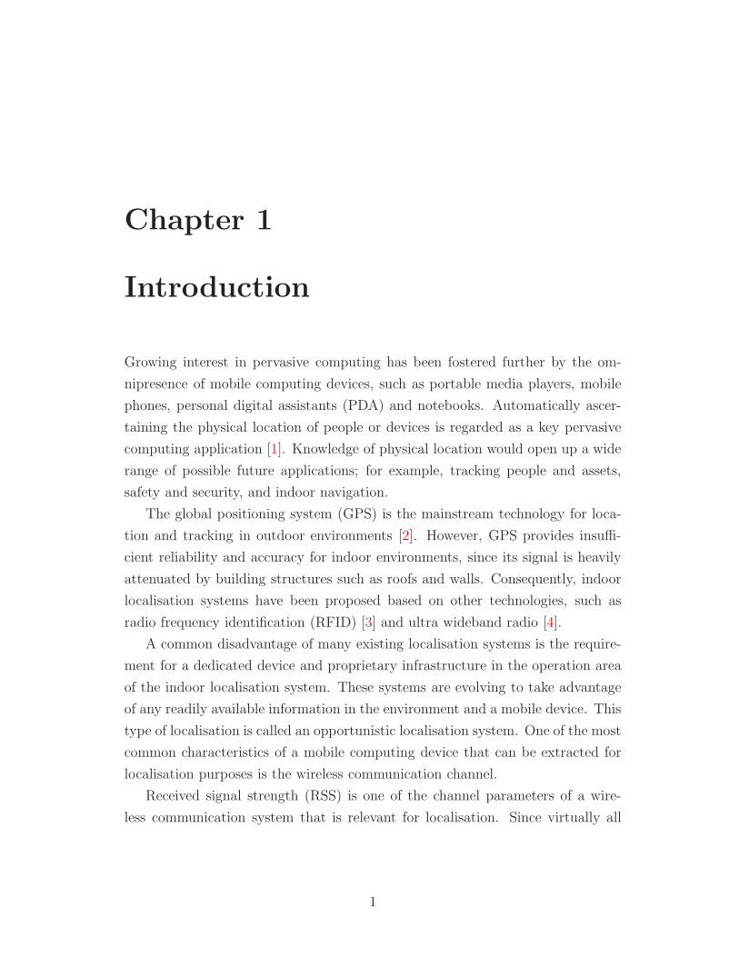
Growing interest in pervasive computing has been fostered further by the om-
nipresence of mobile computing devices, such as portable media players, mobile
phones, personal digital assistants (PDA) and notebooks. Automatically ascer-
taining the physical location of people or devices is regarded as a key pervasive
computing application [1]. Knowledge of physical location would open up a wide
range of possible future applications; for example, tracking people and assets,
safety and security, and indoor navigation.
The global positioning system (GPS) is the mainstream technology for loca-
tion and tracking in outdoor environments [2]. However, GPS provides insuffi-
cient reliability and accuracy for indoor environments, since its signal is heavily
attenuated by building structures such as roofs and walls. Consequently, indoor
localisation systems have been proposed based on other technologies, such as
radio frequency identification (RFID) [3] and ultra wideband radio [4].
A common disadvantage of many existing localisation systems is the require-
ment for a dedicated device and proprietary infrastructure in the operation area
of the indoor localisation system. These systems are evolving to take advantage
of any readily available information in the environment and a mobile device. This
type of localisation is called an opportunistic localisation system. One of the most
common characteristics of a mobile computing device that can be extracted for
localisation purposes is the wireless communication channel.
Received signal strength (RSS) is one of the channel parameters of a wire-
less communication system that is relevant for localisation. Since virtually all
1
1.1 Motivation and Thesis
wireless communication devices are able to obtain and read RSS, the localisation
system can be implemented in the off-the-shelf device with little or no hardware
change. The system becomes a software and algorithmic solution. However, some
aspects of opportunistic indoor localisation systems need to be enhanced, namely
usability1 of the system and accuracy of location estimation. Before a locali-
sation system can be used, system calibration must be performed. During this
calibration, RSS measurements throughout the coverage area must be collected
and saved in a database called a fingerprint.
Building a fingerprint is an expensive undertaking. It is time-consuming and
cumbersome and building a fingerprint in a large-scale indoor environment is
especially labour-intensive. The effort required outweighs the value of having the
localisation system in the first place, thus hindering large scale adoption of such
systems.
1.1 Motivation and Thesis
The development of an algorithm to enhance the accuracy and usability is a
foundation in achieving an affordable, accurate and usable indoor localisation
system. Consequently, this area has received significant research interest in recent
years. However, the proposed solutions are still suboptimal given the problems
they are attempting to address.
The main motivation of the research is to address current drawbacks of the
opportunistic system and to develop a viable algorithm to advance state of the
art of the opportunistic indoor localisation system. It is achieved by enhancing
current approaches based on a particle filter and devising novel algorithms to
enhance accuracy and usability of opportunistic indoor localisation.
1.2 Research Objectives
The main objectives of the research presented here are summarised as follows:
1Usability is defined as the ease to install and to maintain the system.
2
1.3 Contribution
1. A comprehensive review of the state of the art of indoor localisation sys-
tems, with a particular focus on highlighting opportunities for an affordable,
accurate, and usable opportunistic indoor localisation system.
2. Development and evaluation of a filtering algorithm with a Bayesian ap-
proach to enhance the accuracy of opportunistic indoor localisation.
3. Development and evaluation of a learning data fusion algorithm to enhance
the accuracy and usability of opportunistic indoor localisation.
4. Investigation of the sensor data fusion algorithm between different localisa-
tion technologies and also algorithm implementation in different application
domain.
5. Evaluation and comparison of the developed algorithms against current
approaches with a particular focus on the implementation of opportunistic
indoor localisation.
1.3 Contribution
A learning data fusion algorithm is devised to address current problems in op-
portunistic localisation systems. To enable the implementation of a particle filter
into opportunistic indoor localisation, novel motion and measurement models are
developed.
The particle filter-based algorithm is adopted to improve the accuracy of the
opportunistic system. Furthermore, map filtering and backtracking particle filter
algorithm are devised to further improve the accuracy of the opportunistic indoor
localisation system.
One of the most important contributions of this thesis is the self-calibration
fingerprint algorithm. The novelty of the algorithm lies on the ability to automat-
ically build and maintain the fingerprint up-to-date, thus significantly enhance
the usability of the opportunistic indoor localisation.
In addition, the algorithm is used to fuse different sensory data when more
fine-grained accuracy is desirable or when a multi-modal localisation system is re-
quired for different application domains, such as in localisation for first-responders
3

1.4 Thesis Outline
in emergency scenarios. Sensor-specific measurement models are developed to en-
able the fusion.
The application of particle filter-based data fusion for opportunistic indoor
localisation which can also be implemented into different application domain is
one of the original contributions of this research.
It will be demonstrated that this novel algorithm yields significant benefits
not only for improving accuracy but also in the usability of the opportunistic
indoor localisation.
1.4 Thesis Outline
The remainder of this thesis is organised as follows:
• Chapter 2 describes the state of the art in indoor localisation. It will re-
view current systems and algorithms and address current approaches in
opportunistic indoor localisation.
• Chapter 3 discusses one of the contributions of this thesis - a Bayesian ap-
proach for opportunistic indoor localisation. It will present the idea behind
Bayesian inference, and its implementation as the particle filter algorithm.
• Chapter 4 presents the learning data fusion as the major contribution of the
thesis. The proposed algorithms are used to advance further the accuracy
and usability of opportunistic indoor localisation. It will be described how
the algorithm was able to build and refine the fingerprint.
• Chapter 5 describes the sensor data fusion of different localisation technolo-
gies.
• Chapter 6 provides a detailed evaluation of the proposed algorithm.
• Chapter 7 summarises conclusions that can be derived from the work pre-
sented and assesses future perspectives and opportunities for this research.
It also reflects on the overall conclusions that can be drawn from completing
the research presented in this thesis.
4
Chapter 2
State of the Art
A range of localisation systems have been developed to meet distinctive require-
ments of differing applications and operating environments. This domain has
evolved to utilise various physical phenomena and algorithms for location esti-
mation. This chapter describes current approaches towards development of such
localisation systems. Since various localisation systems exist, a localisation clas-
sification taxonomy is developed to make possible a more structured and com-
prehensive review of current approaches.
Section 2.1 describes the classification of localisation systems, which also
presents advantages and disadvantages of each approach. This classification un-
derlines the opportunities for affordable opportunistic indoor localisation systems.
Section 2.2 focuses on current approaches in opportunistic indoor localisa-
tion. It highlights the necessity for an algorithm that enhances the accuracy and
usability of the opportunistic indoor localisation system.
2.1 Classification of Localisation System
A classification was developed using criteria that help to underline the oppor-
tunities for an affordable, accurate, and usable opportunistic indoor localisation
system. These are:
1. Measured phenomena
2. Measured data processing
5
2.1 Classification of Localisation System
3. Performance
2.1.1 Measured Phenomena
Four phenomena which are typically measured to infer location have been iden-
tified:
1. Time of arrival (TOA) and time difference of arrival (TDOA)
2. Angle of arrival (AOA)
3. Received signal strength (RSS)
4. Inertial
Time of Arrival (TOA) and Time Difference of Arrival (TDOA)
Time of arrival (TOA), which is also sometimes called time of flight (TOF), is
the travel time between synchronised transmitting and receiving devices. The
receiver can find the time of arrival by subtracting the time at which the signal
was transmitted from the time at which the signal was received. TOA can be
measured directly using the ultra wideband (UWB) technique [5] [4] or by using
a signalling technique such as spread spectrum [6] [7]. Time difference of arrival
(TDOA) is the time difference of arrival between multiple synchronised transmit-
ters measured at the receiver. GPS is the best-known example of a localisation
system utilising TDOA measurement. Global system for mobile communications
(GSM) localisation can also be implemented using TDOA [8].
The advantage The advantage of TOA and TDOA is that the estimation can
be very accurate (to sub-meter levels). However, the complexity of the hardware
and the time synchronisation required are important disadvantages of localisa-
tion with time measurements [9]. Localisation systems based on this phenomenon
have low affordability.
6
2.1 Classification of Localisation System
Angle of Arrival (AOA)
Angle of arrival (AOA) is a method for obtaining the direction of propaga-
tion of an incident radio-frequency wave. AOA can be measured either with
a mechanically-steered narrow beam width antenna, or with a fixed array of an-
tennas [10] of which the antenna array approach is more common and practical.
Another method for AOA, which has been used for ultrasound waves, is described
in [11]. It used several ultrasound receivers in a device to infer the angle of in-
coming ultrasonic pulse.
The advantage of AOA is that the required number of devices is relatively
low for localisation. Two measurement points are sufficient for two dimensional
(2D) localisation or three measurement points for three dimensional (3D) locali-
sation1. The estimation also can be very accurate. Disadvantages include the
requirement for relatively large and complex hardware and the fact that accuracy
degrades as the mobile target moves further from the measurement unit [12]. The
hardware requirement will make localisation systems based on this phenomenon
have low affordability.
Received Signal Strength (RSS)
RSS is the radio signal power present at the receiver a distance from the trans-
mitter. In general, RSS decreases proportionately with this distance [13]. If
the relationship of distance to signal strength is known, either analytically or
empirically, the distance between two devices can be calculated.
There are several advantages of using RSS for indoor localisation. Firstly, it
can be implemented in wireless communication systems with little or no hardware
change. All that is needed is the capability to obtain and read RSS, which
is provided by virtually all wireless communication devices. The localisation
system can therefore be implemented in off-the-shelf devices. Secondly, it does
not require synchronisation between transmitter and receiver. These advantages
are key factors that contribute to the greater affordability and usability of using
RSS for indoor localisation. The principal disadvantage is that RSS readings
1It assumes a priori knowledge of orientation
7
2.1 Classification of Localisation System
can show large variations due to interference and multipath on the radio channel.
The accuracy is therefore lower than time measurement methods [14].
Inertial
Inertial is a measured phenomenon used to infer the direction, displacement or
velocity of an object for navigational purposes1. A range of instruments can be
utilised for such measurements including accelerometers, magnetometers, gyro-
scopes, compasses or odometers. A more detailed explanation of how the navi-
gational instruments work can be found in [15] [16].
The advantage of using inertial measured phenomena is that the sensors
are independent of any external infrastructure. Therefore, it is suitable for lo-
calisation or navigation where there is no localisation infrastructure inside the
building, such as localisation for first responders [17]. A disadvantage is that
these systems can only provide a relative position; to provide an absolute position
the assistance of another system would be required.
Other
There are a variety of other measured phenomenon that can be used for localisa-
tion, such as images taken from a wearable camera [18] [19] or audio and video
signals [20] as data supplemental to other localisation systems. Since these meth-
ods required specialised and costly hardware, this method has a low affordability.
Therefore, these methods are beyond the scope of the present work and will not
be discussed further here.
2.1.2 Measured Data Processing
Classification based on measured data processing looks into how localisation sys-
tems process measured phenomena to infer location. The most common data
processing methods to infer location are:
1. Geometric
1Navigation is a determination of position and velocity of a moving vehicle.
8
2.1 Classification of Localisation System
2. Fingerprinting
3. Proximity
4. Dead reckoning
Geometric
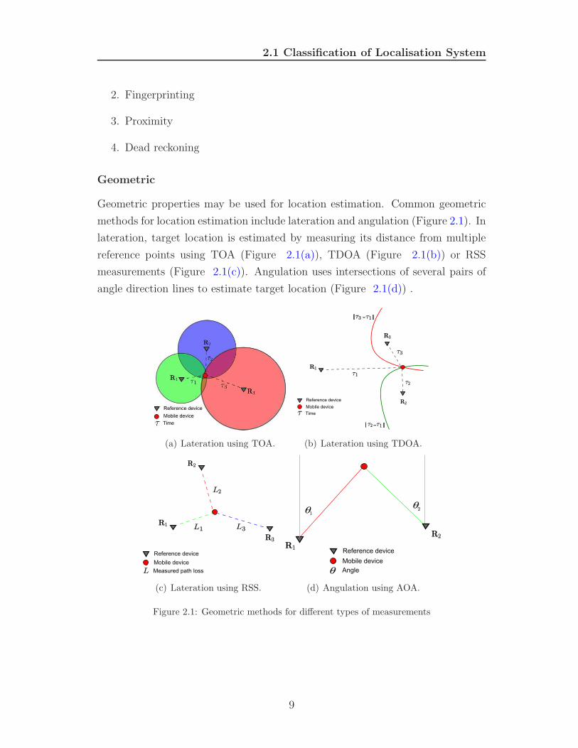
Geometric properties may be used for location estimation. Common geometric
methods for location estimation include lateration and angulation (Figure 2.1). In
lateration, target location is estimated by measuring its distance from multiple
reference points using TOA (Figure 2.1(a)), TDOA (Figure 2.1(b)) or RSS
measurements (Figure 2.1(c)). Angulation uses intersections of several pairs of
angle direction lines to estimate target location (Figure 2.1(d)) .
(a) Lateration using TOA. (b) Lateration using TDOA.
(c) Lateration using RSS. (d) Angulation using AOA.
Figure 2.1: Geometric methods for different types of measurements
9
2.1 Classification of Localisation System
Finding the circles’ intersection points or minimising cost function using the
least-square technique is a straightforward method with TOA [21]. A hyper-
bolic method (Figure 2.1(b)) may be used for TDOA measurements [22] whilst
distances can be calculated from RSS measurements using a radio propagation
model [23].
Fingerprinting
Fingerprinting is a method for mapping measured data (e.g.: RSS) to a known
grid-point throughout the coverage area in the environment. Location is esti-
mated from comparison between real-time RSS measurement and a RSS previ-
ously stored in the fingerprint. Fingerprinting is often used for RSS-based indoor
localisation, especially when analytical correlation between RSS measurement
and distance is not easily established due to multipath and interference [9].
Proximity
The proximity method provides symbolic location in terms of co-location with
a known landmark. Mostly, it relies on the deployment of a dense grid antenna
as the landmark. Mobile device location is determined as the antenna position
which received the strongest signal. The proximity method is widely used for
RFID [3], infra red localisation [24] or GSM positioning with cell identification
(Cell-ID) or cell of origin (COO) method [25].
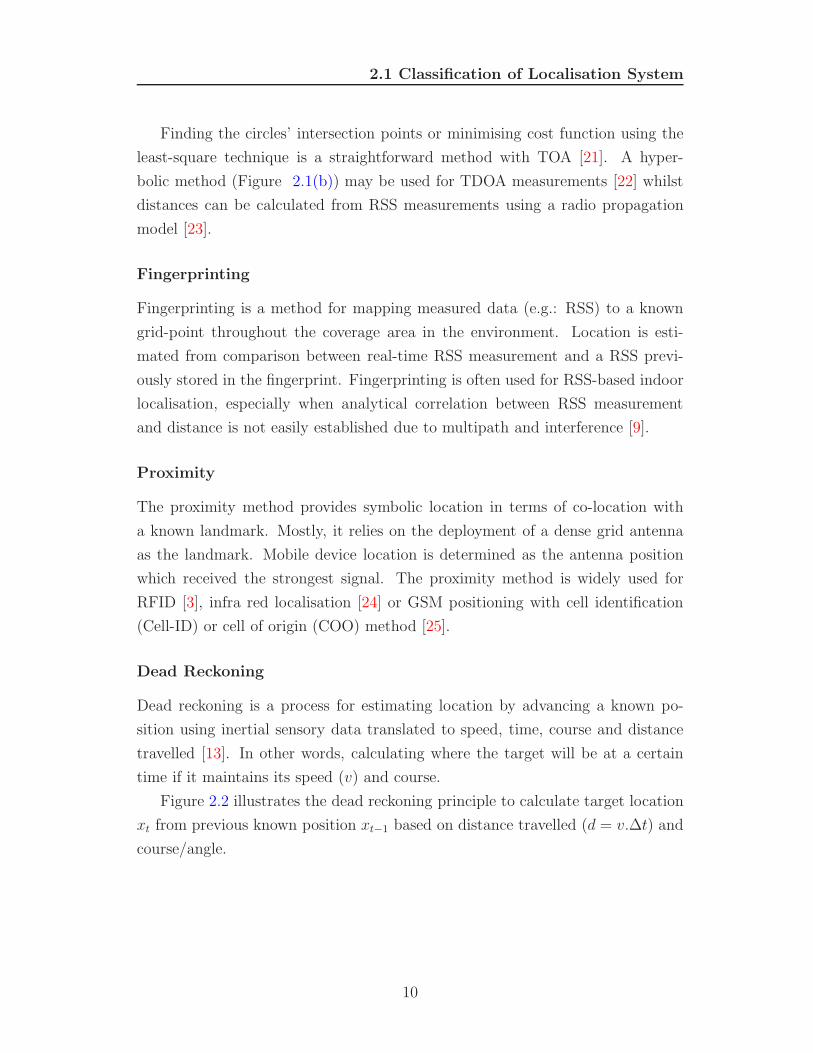
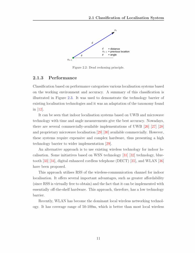
Dead Reckoning
Dead reckoning is a process for estimating location by advancing a known po-
sition using inertial sensory data translated to speed, time, course and distance
travelled [13]. In other words, calculating where the target will be at a certain
time if it maintains its speed (v) and course.
Figure 2.2 illustrates the dead reckoning principle to calculate target location
xt from previous known position xt−1 based on distance travelled (d = v.∆t) and
course/angle.
10
2.1 Classification of Localisation System
Figure 2.2: Dead reckoning principle.
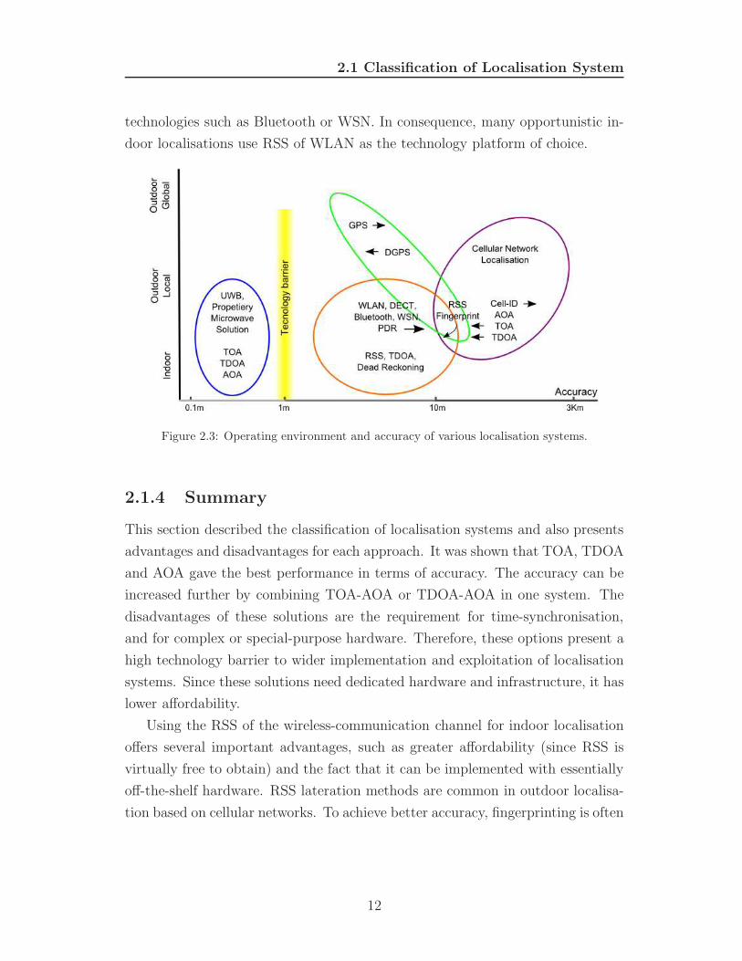
2.1.3 Performance
Classification based on performance categorises various localisation systems based
on the working environment and accuracy. A summary of this classification is
illustrated in Figure 2.3. It was used to demonstrate the technology barrier of
existing localisation technologies and it was an adaptation of the taxonomy found
in [12].
It can be seen that indoor localisation systems based on UWB and microwave
technology with time and angle measurements give the best accuracy. Nowadays,
there are several commercially-available implementations of UWB [26] [27] [28]
and proprietary microwave localisation [29] [30] available commercially. However,
these systems require expensive and complex hardware, thus presenting a high
technology barrier to wider implementation [29].
An alternative approach is to use existing wireless technology for indoor lo-
calisation. Some initiatives based on WSN technology [31] [32] technology, blue-
tooth [33] [34], digital enhanced cordless telephone (DECT) [35], and WLAN [36]
have been proposed.
This approach utilises RSS of the wireless-communication channel for indoor
localisation. It offers several important advantages, such as greater affordability
(since RSS is virtually free to obtain) and the fact that it can be implemented with
essentially off-the-shelf hardware. This approach, therefore, has a low technology
barrier.
Recently, WLAN has become the dominant local wireless networking technol-
ogy. It has coverage range of 50-100m, which is better than most local wireless
11
2.1 Classification of Localisation System
technologies such as Bluetooth or WSN. In consequence, many opportunistic in-
door localisations use RSS of WLAN as the technology platform of choice.
Figure 2.3: Operating environment and accuracy of various localisation systems.
2.1.4 Summary
This section described the classification of localisation systems and also presents
advantages and disadvantages for each approach. It was shown that TOA, TDOA
and AOA gave the best performance in terms of accuracy. The accuracy can be
increased further by combining TOA-AOA or TDOA-AOA in one system. The
disadvantages of these solutions are the requirement for time-synchronisation,
and for complex or special-purpose hardware. Therefore, these options present a
high technology barrier to wider implementation and exploitation of localisation
systems. Since these solutions need dedicated hardware and infrastructure, it has
lower affordability.
Using the RSS of the wireless-communication channel for indoor localisation
offers several important advantages, such as greater affordability (since RSS is
virtually free to obtain) and the fact that it can be implemented with essentially
off-the-shelf hardware. RSS lateration methods are common in outdoor localisa-
tion based on cellular networks. To achieve better accuracy, fingerprinting is often
12
2.2 Current Approaches to Opportunistic Indoor Localisation
preferable, especially when analytical correlation between distance and RSS mea-
surement is difficult to establish, such as in indoor environments. Fingerprinting,
therefore, is method of choice for opportunistic indoor localisation.
The aforementioned advantages make RSS as the phenomenon of choice for
opportunistic indoor localisation. However, the accuracy of RSS-based oppor-
tunistic indoor location still needs to be enhanced to meet requirements of typi-
cal applications. Furthermore, building an RSS fingerprint is not a trivial effort,
especially in large scale indoor environment.
Enhancing the accuracy and usability of opportunistic indoor localisation be-
comes the objective of this research. Furthermore, using single type of measured
phenomenon may not offer required accuracy, but they can be combined to achieve
better accuracy.
WLAN has become the dominant local wireless networking technology. Ac-
cordingly, majority of the opportunistic indoor localisation systems use RSS of
WLAN as the technology platform. The next section will review current ap-
proaches in opportunistic indoor localisation and identify problems that still need
to be addressed.
2.2 Current Approaches to Opportunistic In-
door Localisation
There have been considerable research in the area of opportunistic indoor locali-
sation particularly using WLAN as the technology platform. There are a number
of methods commonly used to infer location from RSS measurement. Those
methods will be presented in the following section.
2.2.1 Current Methods
Nearest Neighbour (NN)
An early implementation, called RADAR [36], adopted a method termed nearest
neighbour (NN) distance in signal space. The location is estimated by a position
13
2.2 Current Approaches to Opportunistic Indoor Localisation
in the fingerprint which has smallest distance (d∗). The distance is governed by
the following expressions:
d∗ = arg minz+∈Z+
M(z+, z) (2.1)
with
M(z+, z) =∑
k∈(z+∩z)
|z+k − zk| (2.2)
where d∗ represents the distance, Z+ represents the fingerprint, z+and z represent
a set of RSS in the fingerprint and measurement, respectively, k represents WLAN
the access point (AP), z+kand zk represent the RSS value in the fingerprint and
measurement, respectively.
The authors offered two approaches to building a fingerprint. First, make
empirical measurements of RSS data throughout the coverage area in the indoor
environment. Second, using a propagation model called multi-wall model (MWM)
as suggested in [37]. Fingerprint prediction with a propagation model is explained
in more detail in section 2.2.3.
The advantage of the NN method is its simplicity and its requirement for
relatively low amount of computational power. The Disadvantages of the NN
methods are that it only takes into account current measurements to estimate
target location, and ignores other information (such as target behaviour, previous
measurements, etc.). This approach often leads to poor estimation accuracy.
Motetrack
Motetrack [38] is a RSS-based indoor localisation using WSN as the technology
platform. It uses a decentralised approach that runs on programmable beacon
nodes. The fingerprint database is replicated across the beacon nodes to minimise
per-node storage overhead and to achieve high robustness to failure.
To infer location, Motetrack extends NN method with a concept of penalty,
termed adaptive signature distance metric. The distance metric is governed by:
d∗ = arg minz+∈Z+
M(z+, z) (2.3)
14
2.2 Current Approaches to Opportunistic Indoor Localisation
with
M(z+, z) =∑
k∈(z+∩z)
|z+k − zk| +∑
k∈(z+−z)
z+k +∑
k∈(z−z+)
zk (2.4)
where d∗ represents the distance, Z+ represents the fingerprint, z+and z rep-
resent a set of RSS in the fingerprint and measurement, respectively, k represents
a WSN beacon node, z+kand zk represent the RSS value in the fingerprint and
measurement, respectively. The advantages of the Motetrack method is its sim-
plicity and speed. The decentralised characteristic also makes it robust to failure.
The disadvantage of the Motetrack is, like NN method, its simple approach to
calculate the distance metric often leads to poor estimation accuracy.
Placelab
Placelab [39] tries to reduce barrier-to-entry to localisation systems by construct-
ing community contributed radio-map. Radio map is a database of beacons po-
sition (GSM towers and WLAN APs).
Many of these beacon databases come from institutions that own a large
number of wireless networking beacons or databases produced by the war-driving
community. War-driving is the act of driving around with a mobile computer
equipped with a GPS device and a radio (typically a WLAN card but sometimes
a GSM phone or Bluetooth device) to collect beacons position.
Distance to known beacons position in the database is inferred by RSS-
lateration method. The location can be calculated with finding the circles’ inter-
section points similarly used in TOA (see section 2.1.2).
The advantages of Placelab is that it can be used to integrate outdoor
and indoor localisation. The effort to build the radio map is also low since it is a
community contributed database. The disadvantage is that it has low accuracy
(15-20m).
Machine Learning
A machine learning approach has also been used for opportunistic indoor local-
isation. An artificial-neural-network (ANN) based classifier was used to infer
15
2.2 Current Approaches to Opportunistic Indoor Localisation
location from WLAN RSS [40]. The fingerprint is used as training data for
ANN to build the localisation estimation model. The aforementioned study uses
three-layer architecture with three input units, eight hidden layer units, and two
outputs.
In [41] and [42], the authors proposed a statistical learning method based
on the support vector machine (SVM) classifier. SVM is a supervised learning
method which is mostly used as classification/regression. It uses a fingerprint as
its training data to build a classification model. During the training phase, SVM
constructs a classifier termed as hyper-plane which in turn is used to estimate
the target location.
An important disadvantage of the machine learning approach is that it
makes several assumptions which may not hold true in all situations [43]. Firstly,
it requires large amounts of labelled data1 to train the system. Secondly, the
learned localisation model is static over time and across space. Moreover, static
location estimation and tracking of moving targets will give significantly differ-
ent results as this method does not properly consider a kinematic model of the
target [12].
Horus
The Horus system [44] [45] proposed a joint clustering technique for location
estimation. Each candidate location is regarded as a class or category. The
fingerprint was stored as a collection of models for the joint probability distri-
butions. The fingerprint is built using probabilistic aggregation, either based
on a histogram method or on a kernel distribution method [46]. The estimated
location is calculated by:
arg maxx
P (x|z) = arg maxx
P (z|x).P (z) (2.5)
where P (x|z) represents conditional probability of location x given measure-
ment z, P (z|x) represents conditional probability of measurement z given location
x, P (z) represents probability of measurement z.
1RSS with ground truth position, analogue to a fingerprint
16
2.2 Current Approaches to Opportunistic Indoor Localisation
The advantage of the Horus method is it can reduce required computational
power by the clustering technique. Disadvantages of the Horus is it needs a large
training data set (fingerprint) to properly construct the joint cluster. Therefore,
it has poor usability. It also does not consider kinematic behaviour of target and
assumed that the cluster probability always has Gaussian distribution, which can
lead to reduced accuracy.
Kalman Filter
The Kalman filter is a probabilistic method based on Bayesian filter. It approxi-
mates the probability distribution of the target location by a Gaussian represen-
tation. It has been widely used in robotic mapping and localisation [47] [48]. The
probability distribution is given by [49]:
p(xt|zt) ≈ N(xt; µt, Et) (2.6)
=1
(2π)d/2|Et|1/2exp
[
−1
2(xt − µt)
T E−1t (xt − µt)
]
(2.7)
where µt is the mean of the distribution, Et is the d x d covariance matrix, d
represents state’s dimension. N(xt; µt, Et) denotes the probability of xt given a
Gaussian with mean µt and covariance Et.
The principal advantages of Kalman filter lie in their computational effi-
ciency compared to other variants of Bayesian filters. It is also suitable for systems
with an accurate sensor measurement. A major disadvantage is that it only can
represent unimodal Gaussian distribution and it only suitable in a system which
has linear observation model and system dynamics.
Particle Filter
Among the family of Bayesian filtering, the most powerful algorithm comes from
a Monte Carlo methods implemented as a particle filter. In [50], particle filtering
is compared to other state of the art algorithms and it gives the best performance
for state estimation. The particle filter robustness lies in the ability to handle
non-linear system with non-Gaussian noise. The particle filter has been widely
implemented in robotic localisation [49] [51].
17
2.2 Current Approaches to Opportunistic Indoor Localisation
The principal advantages of particle filter lie in its ability to handle non-
linear system with non-Gaussian noise. The ability to incorporate a kinematic
of the moving target and its inherent ability to combine various sensor measure-
ments in its probability model make this method is naturally suitable for sensor
data fusion. The disadvantage is that it requires relatively high computational
power.
2.2.2 Accuracy and Sensor Data Fusion
Accuracy
Each method (described in section 2.2.1 previously) has its own claim about
system performance in terms of accuracy. However, it can be problematic to
compare the performance of different methods by this criterion, since they are
usually implemented in different environments and with differing data sets. An
attempt has been made to compare SVM with other methods, such as ANN, kNN
and Bayesian probability in the same experimental platform [42].
The SVM method gave an accuracy of 3.96m with 75% probability, the ANN
gave an accuracy of 4.01m with 75% probability and the kNN gave a value of
3.98m with 75% probability. In [52], the author developed a localisation test-bed
for independently evaluating Ekahau1 software [53] in a laboratory setting. He
reported an x-axis Cartesian error of 5m and y-axis of 4.6m in a typical office
environment with 7 APs.
Sensor Data Fusion
The accuracy of a single technology alone often cannot satisfy requirements for a
higher degre of accuracy. For such situations, an additional localisation technol-
ogy can help improve accuracy by means of sensor data fusion.
Fusion is defined as a technique to combine data from multiple sensors with
related information from associated databases, to achieve improved accuracy and
more specific inferences than could be achieved by the use of a single sensor alone.
1Ekahau is a commercial WLAN-based indoor localisation.
18
2.2 Current Approaches to Opportunistic Indoor Localisation
The data can come from sensors, history values of sensor data, information
sources like a priori knowledge about the environment and human input [54] [55].
Most of the work on the sensor data fusion was performed in the field of
robotic localisation [56] [57].
2.2.3 Limitations of the Fingerprinting Method
Another drawback of opportunistic localisation based on RSS measurements is
the necessity to build a fingerprint. Building a fingerprint database is an exhaus-
tive, time-consuming and cumbersome effort. Furthermore, a fingerprint is also
bound to the indoor environment description and infrastructure at the time the
fingerprint was generated. Therefore, major changes in the environment (move-
ment of large pieces of furniture or appliances, adding or removing walls) will
render a current fingerprint inaccurate and require re-building of a new finger-
print. In other words, the current approach still has poor usability, evaluated from
the effort needed to install and maintain it.
There are two main approaches to overcome this problem: fingerprint predic-
tion with a propagation model and fingerprint modelling with a machine learning
approaches.
Fingerprint Prediction with Propagation Model
In [36] [58] [59] various propagation models such as one slope model (OSM) [60],
multi wall model (WWM) and motif ray tracing model (MM) [61] have been used
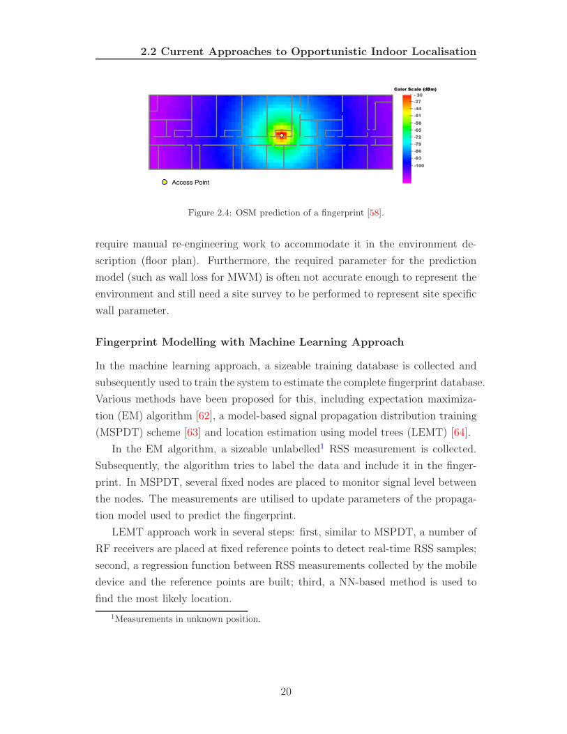
to predict the fingerprint. Figure 2.4 gives an example of a fingerprint prediction
with the OSM model. The signal loss in OSM is given by:
L = L1 + 10nlog(d) (2.8)
where L is a signal loss, L1 (dB) is a reference loss value of 1m distance, n is a
power decay factor (path loss exponent) defining slope, and d is the distance in
meters.
The principal advantage of fingerprint prediction is its speed in predicting
the fingerprint compared to the measured fingerprint. A key disadvantage is
that changes to the indoor environment (such as wall addition or removal) will
19
2.2 Current Approaches to Opportunistic Indoor Localisation
Figure 2.4: OSM prediction of a fingerprint [58].
require manual re-engineering work to accommodate it in the environment de-
scription (floor plan). Furthermore, the required parameter for the prediction
model (such as wall loss for MWM) is often not accurate enough to represent the
environment and still need a site survey to be performed to represent site specific
wall parameter.
Fingerprint Modelling with Machine Learning Approach
In the machine learning approach, a sizeable training database is collected and
subsequently used to train the system to estimate the complete fingerprint database.
Various methods have been proposed for this, including expectation maximiza-
tion (EM) algorithm [62], a model-based signal propagation distribution training
(MSPDT) scheme [63] and location estimation using model trees (LEMT) [64].
In the EM algorithm, a sizeable unlabelled1 RSS measurement is collected.
Subsequently, the algorithm tries to label the data and include it in the finger-
print. In MSPDT, several fixed nodes are placed to monitor signal level between
the nodes. The measurements are utilised to update parameters of the propaga-
tion model used to predict the fingerprint.
LEMT approach work in several steps: first, similar to MSPDT, a number of
RF receivers are placed at fixed reference points to detect real-time RSS samples;
second, a regression function between RSS measurements collected by the mobile
device and the reference points are built; third, a NN-based method is used to
find the most likely location.
1Measurements in unknown position.
20
2.2 Current Approaches to Opportunistic Indoor Localisation
The LEMT method is generally similar to the MSPDT method with the differ-
ence being that instead of using an indoor propagation model, it uses a machine
learning approach to learn regression relationship between RSS and location to
build a complete fingerprint.
These proposed methods offer a considerable advantage in that collection
of the empirical fingerprint data is significantly reduced. In [62], the machine
learning method used 50-75% less data compared to the empirical fingerprint.
The disadvantage of the method is that the learned localisation model is static
over time and/or across space. The model will therefore be rendered inaccurate if
there are changes to the propagation environment or used in other environments.
The system needs then to be re-trained with an updated training database to
reflect the changes. In MSPDT and LEMT, a numbers of dedicated RF receivers
are required to monitor RSS values all time (4-8 devices in their experiments).
2.2.4 Summary
This section described a detailed review of various methods that commonly used
to infer location from RSS measurement. Based on the state of the art, the
particle filter algorithm has been identified as the most viable method for the
opportunistic system. The particle filter robustness lies in the ability to handle
non-linear systems with non-Gaussian noise. The particle filter has been widely
implemented in robotic localisation.
The accuracy of a single technology alone often cannot satisfy requirements for
a higher granularity of accuracy. For such situations, an additional localisation
technology can help improve accuracy by means of sensor data fusion.
A disadvantage of opportunistic localisation based on RSS measurement is
the necessity to build a fingerprint. Building a fingerprint data base is an ex-
haustive, time-consuming and cumbersome effort. Furthermore, a fingerprint is
also bound to the indoor environment description and infrastructure at the time
the fingerprint was generated.
To address the fingerprinting problem, current methods use indoor propaga-
tion modelling or machine learning approach. Nevertheless, the proposed solu-
21
2.3 Summary of Motivation
tions still have many disadvantages which hinder them from fully addressing the
usability problem of the opportunistic system.
2.3 Summary of Motivation
This chapter described the state of the art of current approaches to indoor local-
isation. The developed taxonomy is utilised to help describe the current state of
development of indoor localisation and underlines opportunities for an affordable,
accurate, and usable opportunistic indoor localisation system. It was shown that
localisation system based on time and angle measurement (TOA, TDOA and
AOA) gave best performance in terms of accuracy. However, these solutions need
dedicated hardware and infrastructure, therefore, it has lower affordability.
Utilising the RSS of the wireless-communication channel for opportunistic
indoor localisation offers several advantages, such as affordability (since RSS is
virtually free to obtain) and a low technology barrier to implementation (sec-
tion 2.1). WLAN has become the dominant local wireless networking technology.
Accordingly, opportunistic indoor localisation uses RSS of WLAN as the tech-
nology platform of choice.
However, there are some aspects of the current approaches in opportunistic
indoor localisation that need to be addressed with more research; namely, further
improvement in the accuracy and usability of the system. Furthermore, sensor
data fusion capability is often overlooked in current approaches, even though
accuracy of a single technology platform often cannot satisfy application require-
ments.
Some algorithms try to enhance the accuracy and to address the usability
problem (section 2.2). However, the proposed solutions still have many disad-
vantages which restrict them from fully addressing the usability problem of the
opportunistic system.
Hence, the drawbacks highlighted in the detail review of the state-of-the-art
compound the need to enhance the accuracy and usability of opportunistic indoor
localisation system.
It was found that the most advanced algorithm is the particle filter which
comes from the family of Monte Carlo methods. This thesis offers a solution
22
2.3 Summary of Motivation
of the accuracy problem by adopting a particle filter approach to opportunistic
localisation (chapter 3).
This research also constructs novel algorithms for enhancing not only the
accuracy but also the usability of opportunistic localisation (chapter 4). Further-
more, the algorithm is able to become a framework for the sensor data fusion
between multi modal localisation technologies to improve the accuracy of indoor
localisation system (chapter 5).
The collection of algorithms to improve the accuracy and usability of oppor-
tunistic indoor localisation system are the primary contribution of this thesis.
The first contribution, that is the adoption of particle filter algorithm to oppor-
tunistic indoor localisation, will be described further in the next chapter.
23
Chapter 3
Particle Filter for Localisation
Based on the comprehensive review of the state of the art, it was found that the
particle filter is the most advance algorithm. To achieve one of the thesis objec-
tives, which is improving the accuracy, the particle filter algorithm is adopted to
the opportunistic indoor localisation.
This chapter will describe the Bayesian probability approach implemented as
the particle filter algorithm for opportunistic indoor localisation. Section 3.1 and
3.2 will present the theory that underlies the particle filter.
To enable the implementation of a particle filter into opportunistic indoor
localisation, motion and measurement models have to be devised beforehand.
These probabilistic models are one of the contributions of this research, which
will be explained in section 3.4 and section 3.5 in more detail. Section 3.7 will
conclude the chapter.
3.1 State Estimation
In order to clearly describe the problem during localisation, some terms are used
in the following chapters. These are defined here for clarity and convenience.
Firstly, target, is defined as an entity (e.g.: object, person) of which the state is
being estimated. For example, it can be a person to whom the located mobile
device is attached. Secondly state, is defined as the collection of the aspect of the
target (such as location, velocity, or direction). The state will change over time.
Thirdly, measurement, the observed phenomena obtained from a sensor which
24
3.1 State Estimation
carries information about the state. RSS measurement is utilised for opportunistic
indoor localisation.
The main goal of an indoor localisation system is to estimate an unknown
target’s state based on the observed measurement. To conveniently describe the
evolution of target state and its measurement during localisation, a statistical
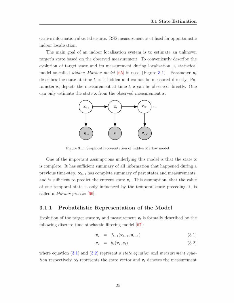
model so-called hidden Markov model [65] is used (Figure 3.1). Parameter xt
describes the state at time t, x is hidden and cannot be measured directly. Pa-
rameter zt depicts the measurement at time t, z can be observed directly. One
can only estimate the state x from the observed measurement z.
Figure 3.1: Graphical representation of hidden Markov model.
One of the important assumptions underlying this model is that the state x
is complete. It has sufficient summary of all information that happened during a
previous time-step. xt−1 has complete summary of past states and measurements,
and is sufficient to predict the current state xt. This assumption, that the value
of one temporal state is only influenced by the temporal state preceding it, is
called a Markov process [66].
3.1.1 Probabilistic Representation of the Model
Evolution of the target state xt and measurement zt is formally described by the
following discrete-time stochastic filtering model [67]:
xt = ft−1(xt−1,nt−1) (3.1)
zt = ht(xt, et) (3.2)
where equation (3.1) and (3.2) represent a state equation and measurement equa-
tion respectively, xt represents the state vector and zt denotes the measurement
25
3.1 State Estimation
vector, ft−1 and ht are known, possibly non-linear, time-varying functions, nt−1
and et are independent and identically-distributed noise.
The evolution of state and measurement is governed by a probabilistic prin-
ciple. In order to obtain xt and zt, probabilistic distributions, from which xt and
zt can be generated, must be specified. In general, xt is stochastically generated
from the previous state xt−1. Since the system is assumed to be Markovian, the
previous state xt−1 is a summary of past states and measurements and is sufficient
to predict the current state xt. This can be expressed in the following equation:
p(xt|x0:t−1, z1:t−1) = p(xt|xt−1) (3.3)
In probabilistic terms, this insight is called transition probability. Transition
probability is a stochastic representation of equation (3.1).
The measurement also can be modelled as a conditional probability of the
state xt. Once again, since xt is complete, it is enough to utilise xt to predict the
potentially noisy measurement zt. The measurement model can be written as:
p(zt|x0:t, z1:t−1) = p(zt|xt) (3.4)
Equation (3.4) is called the measurement probability. It is a probabilistic repre-
sentation of equation (3.2).
Another important concept of the probabilistic representation for the HMM
is posterior probability and prior probability. Posterior probability represents
probability distribution of state xt given all available measurements. It assigns a
probabilistic value to each hypothesis of the true state. Posterior probability is
expressed by:
p(xt|z1:t) = p(xt|zt) (3.5)
This density is the probability distribution over state xt at time t, given all past
measurements z1:t.
Prior probability is a probability calculated based on the previous posterior,
before incorporating measurement at the time t or denoted as zt. This probability
is often referred to as a prediction since it is calculated from the previous posterior.
The prediction probability can be written as:
p(xt|z1:t−1) = p(xt|zt−1) (3.6)
26
3.2 Recursive Bayesian Filtering
Posterior probability can be calculated from the prior by correcting it with the
new measurement zt. This step is often called measurement update or correction.
There are terms that need to be clarified before moving further. Filtering
refers to state estimation xt using measurements up to time t, i.e. {z1, z2, z3, . . . , zt}.Prediction is an a priori form of estimation, using measurement available before t.
Smoothing is estimation using measurements available after t [68].
3.2 Recursive Bayesian Filtering
The general algorithm for calculating the posterior distribution of p(xt|zt) is
given by Bayes’ filter. From a Bayesian perspective, construction of posterior
probability is achieved in two steps: prediction and update. The prediction stage
is performed to obtain the prior probability p(xt|zt−1), whereas the update stage
corrects the prediction with a new measurement to obtain the posterior p(xt|zt).
The prediction is achieved through the the Chapman-Kolmogorov equation [69]:
p(xt|zt−1) =
∫
p(xt|xt−1)p(xt−1|zt−1)dxt−1 (3.7)
When the measurement zt becomes available, Bayes’ rule is utilised for the update
stage:
p(xt|zt) = k−1p(zt|xt)p(xt|zt−1) (3.8)
with normalizing constant:
k =
∫
p(zt|xt)p(xt|zt−1)dxt (3.9)
p(zt|xt) represents the measurement probability, p(xt|xt−1) is the transition prob-
ability and p(xt|zt−1) is the previous posterior probability.
Algorithm 3.1 describes the prediction and update stages of Bayes’ filter. The
algorithm input is the previous posterior and a current measurement. In line 2,
prediction is obtained by integration of two probability distributions: previous
posterior and transition probability. The measurement update is described in line
3, where Bayes’ algorithm updates the prior probability with the measurement
probability. The result is the posterior probability which is returned in line 5
27
3.3 Particle Filter
Algorithm 3.1 BayesFilter (p(xt−1|zt−1), zt)
1: for all xt do
2: p(xt|zt−1)=∫
p(xt|xt−1) p(xt−1|zt−1)dxt−1
3: p(xt|zt)= k−1p(zt|xt) p(xt|zt−1)
4: end for
5: return p(xt|zt)
of the algorithm. The recursive nature of the Bayesian filter is due to the fact
that the posterior probability p(xt|zt) is calculated form the previous posterior
p(xt−1|zt−1).
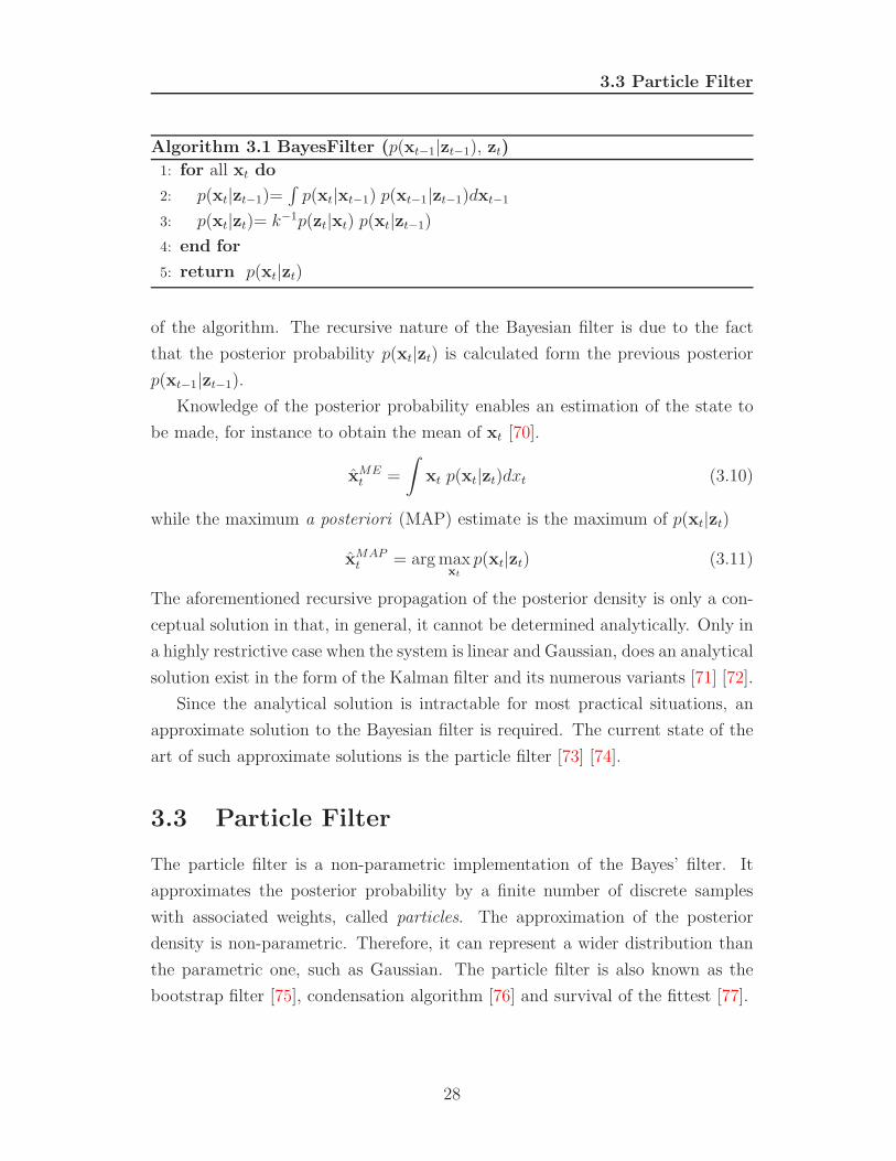
Knowledge of the posterior probability enables an estimation of the state to
be made, for instance to obtain the mean of xt [70].
xMEt =
∫
xt p(xt|zt)dxt (3.10)
while the maximum a posteriori (MAP) estimate is the maximum of p(xt|zt)
xMAPt = arg max
xt
p(xt|zt) (3.11)
The aforementioned recursive propagation of the posterior density is only a con-
ceptual solution in that, in general, it cannot be determined analytically. Only in
a highly restrictive case when the system is linear and Gaussian, does an analytical
solution exist in the form of the Kalman filter and its numerous variants [71] [72].
Since the analytical solution is intractable for most practical situations, an
approximate solution to the Bayesian filter is required. The current state of the
art of such approximate solutions is the particle filter [73] [74].
3.3 Particle Filter
The particle filter is a non-parametric implementation of the Bayes’ filter. It
approximates the posterior probability by a finite number of discrete samples
with associated weights, called particles. The approximation of the posterior
density is non-parametric. Therefore, it can represent a wider distribution than
the parametric one, such as Gaussian. The particle filter is also known as the
bootstrap filter [75], condensation algorithm [76] and survival of the fittest [77].
28
3.3 Particle Filter
The particle filter directly estimates the posterior probability of the state
expressed in the following equation [74]:
p(xt|zt) ≈N
∑
i=1
wtδ(xt − xit) (3.12)
where xit is the i-th sampling point or particle of the posterior probability with
1 < i < N and wit is the weight of the particle. N represents the number of
particles in the particle set, denoted by Xt.
Xt := x1t ,x
2t ,x
3t , . . . ,x
Nt (3.13)
Each particle is a concrete instantiation of the state at time t, or put differ-
ently, each particle is a hypothesis of what the true state xt might be, with a
probability given by its weight.
The property of equation (3.12) holds for N ↑ ∞. In the case of finite N ,
the particles are sampled from a slightly different distribution. However, the
difference is negligible as long as the number of particles is not too small [65].
Based on recent finding [74], N value above 500 is suggested. In this work, N
value of 1000 is used and remain static over time.
Algorithm 3.2 Particle Filter (Xt−1, zt)
1: Xt = Xt = ∅2: for i = 1 to N do
3: sample xit ∼ p(xt|xi
t−1)
4: assign particle weight wit = p(zt|xi
t)
5: end for
6: calculate total weight k =∑N
i=1 wit
7: for i = 1 to N do
8: normalise wit = k−1wi
t
9: Xt = Xt + {xit, w
it}
10: end for
11: Xt = Resample (Xt)
12: return Xt
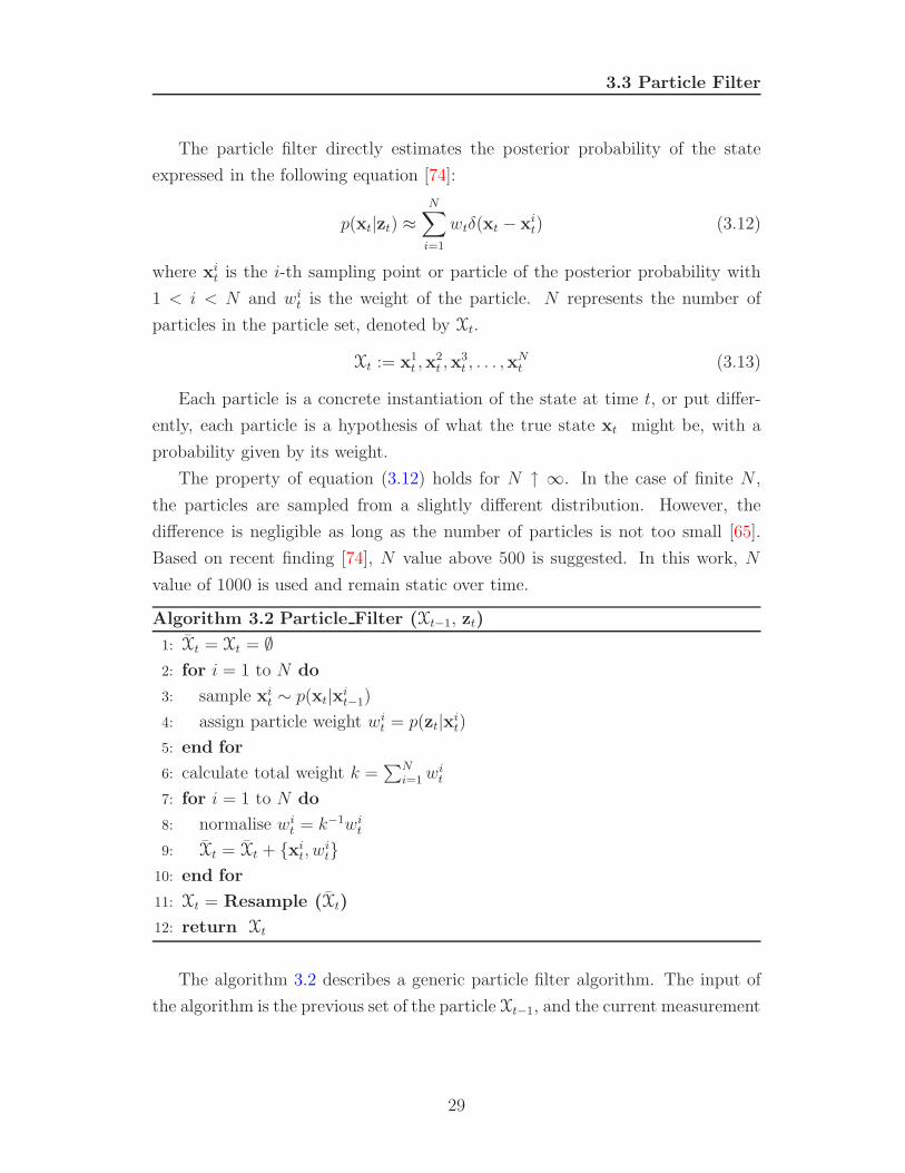
The algorithm 3.2 describes a generic particle filter algorithm. The input of
the algorithm is the previous set of the particle Xt−1, and the current measurement
29
3.3 Particle Filter
zt, whereas the output is the recent particle set Xt. The algorithm will process
every particle xit−1 from the input particle Xt−1 as follows.
1. Line 3 shows the prediction stage of the filter. The particle xit is sampled
from the transition distribution p(xt|xt−1). The set of particles resulting
from this step has a distribution according to (denoted by ∼) the prior
probability p(xt|zt−1).
2. Line 4 describes incorporation of the measurement zt into the particle. It
calculates for each particle xit the importance factor or weight wi
t. The
weight is the probability of particle xit received measurement zt or p(zt|xt).
The construction process of the weight will be described in section 3.5.
3. Lines 7 to 10 are steps required to normalise the weight of the particles.
The result is the set of particles Xt, which is an approximation of posterior
distribution p(xt|zt).
4. Line 11 describes the step which is known as resampling or importance re-
sampling. The resampling procedure is described in algorithm 3.3 in the
next section. After the resampling step, the particle set, which was previ-
ously distributed in a manner equivalent to prior distribution p(xt|zt−1) will
now be changed to particle set Xt which is distributed in proportion to
p(xt|zt).
3.3.1 Resampling
The early implementation of particle filter is called sequential important sampling
(SIS) [78]. Implementation of SIS is similar to algorithm 3.2, but without the
resample step (algorithm 3.2 line 11). The SIS approach suffers an effect which
is called the degeneracy problem.
This occurs when, after some sequence time t, all but one particle has nearly
zero weight. The problem happen since generally impossible to sample directly
from posterior distribution, particles are sampled from related distribution, termed
importance sampling. The choice of importance sampling made the degeneracy
30

3.3 Particle Filter
problem is unavoidable [79]. The degeneracy problem will increase the weight
variance over time and has a harmful effect on accuracy [74].
Resampling is an important step to overcome the degeneracy problem. It will
force the particle to distribute according to the posterior density p(xt|zt).
Algorithm 3.3 Resample (Xt)
1: X∗t = ∅
2: for j = 1 to N do
3: r = random number uniformly distributed on [0,1]
4: s = 0.0
5: for i = 1 to N do
6: s = s + wit
7: if s ≥ r then
8: x∗jt = xi
t
9: w∗jt = 1/N
10: X∗t = X
∗t + {x∗j
t , w∗jt }
11: end if
12: end for
13: end for
14: replacement Xt = X∗t
15: return Xt
Algorithm 3.3 describes a resampling step of particles. It is taken with a slight
modification from [80] to increase the efficiency of the method. The modification
lies in the iteration to draw newly sampled particles. The input of the algorithm
is a set of particles and the output is the new resampled particles.
1. Line 3 shows the generation of random number r.
2. Lines 5 to 8 show the resampling steps. Line 8 shows when a particle is
resampled only if its weight contribution causes the summation in line 6
to exceed or equal to the random sample r. The probability of drawing1
a particle is in proportion to its importance factor. Particles with lower
weight will have a lower chance and some will not be resampled.
1Random selection
31
3.3 Particle Filter
3. Since the resampling process is performed every time step, the new particles
do not need to know the old weight and their weight will be set equally, as
shown in line 9.
4. Line 14 shows when members of particle set Xt is replaced by new resampled
particles.
Although the resampling step reduces the effects of the degeneracy prob-
lem, it introduces other practical problems. Firstly, it limits the opportunity to
implement the algorithm on a parallel computer since all the particles must be
combined. Secondly, the particles that have high weights are statistically selected
many times. This leads to a loss of diversity among the particles as the resultant
sample will contain many repeated points.
This problem, which is known as sample impoverishment, is apparent when
process noise in state dynamics is small1. If the process noise is zero, then using a
particle filter is not entirely appropriate. Particle filtering is a method well suited
to the estimation of dynamic states.
State dynamics of RSS-based opportunistic indoor localisation is large due
to noisy RSS measurement. Therefore, particle filter is well suited for state
estimation in opportunistic system.
3.3.2 Summary
The particle filter, which is a non-parametric implementation of Bayes’ filter, is
well suited for state estimation in opportunistic system for a number of reasons.
Firstly, it is the state of the art algorithm for a non-linear system with non-
Gaussian noise such as in RSS-based opportunistic indoor localisation. Secondly,
it is suitable for state estimation for a system that has large process noise in state
dynamics. Thirdly, the particle filter is the most powerful algorithm to date to
improve the performance of an opportunistic system.
To enable the implementation of a particle filter into opportunistic indoor lo-
calisation, motion and measurement model have to be devised beforehand. These
probabilistic models will be explained in section the following sections.
1Smoothing is one of the approaches to overcome sample impoverishment [81]
32
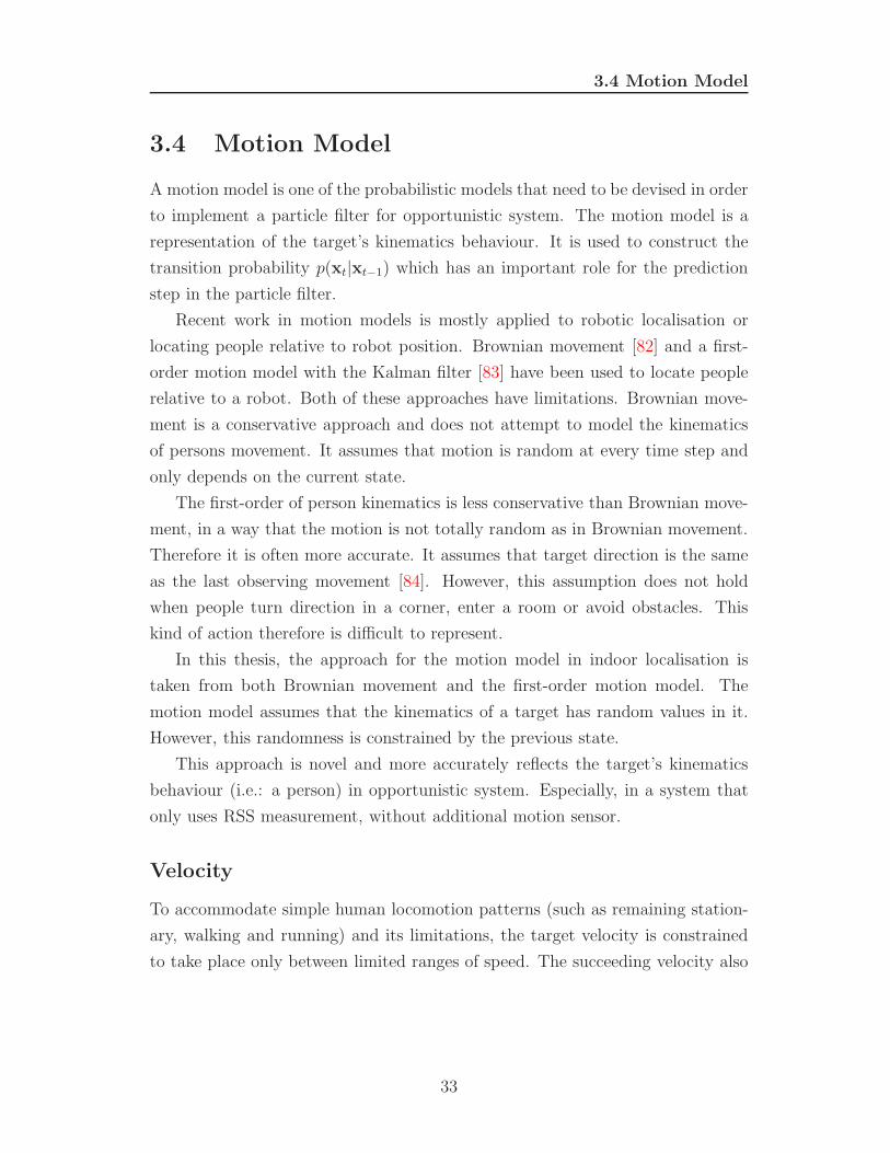
3.4 Motion Model
3.4 Motion Model
A motion model is one of the probabilistic models that need to be devised in order
to implement a particle filter for opportunistic system. The motion model is a
representation of the target’s kinematics behaviour. It is used to construct the
transition probability p(xt|xt−1) which has an important role for the prediction
step in the particle filter.
Recent work in motion models is mostly applied to robotic localisation or
locating people relative to robot position. Brownian movement [82] and a first-
order motion model with the Kalman filter [83] have been used to locate people
relative to a robot. Both of these approaches have limitations. Brownian move-
ment is a conservative approach and does not attempt to model the kinematics
of persons movement. It assumes that motion is random at every time step and
only depends on the current state.
The first-order of person kinematics is less conservative than Brownian move-
ment, in a way that the motion is not totally random as in Brownian movement.
Therefore it is often more accurate. It assumes that target direction is the same
as the last observing movement [84]. However, this assumption does not hold
when people turn direction in a corner, enter a room or avoid obstacles. This
kind of action therefore is difficult to represent.
In this thesis, the approach for the motion model in indoor localisation is
taken from both Brownian movement and the first-order motion model. The
motion model assumes that the kinematics of a target has random values in it.
However, this randomness is constrained by the previous state.
This approach is novel and more accurately reflects the target’s kinematics
behaviour (i.e.: a person) in opportunistic system. Especially, in a system that
only uses RSS measurement, without additional motion sensor.
Velocity
To accommodate simple human locomotion patterns (such as remaining station-
ary, walking and running) and its limitations, the target velocity is constrained
to take place only between limited ranges of speed. The succeeding velocity also
33
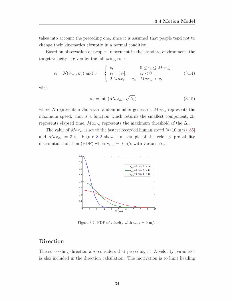
3.4 Motion Model
takes into account the preceding one, since it is assumed that people tend not to
change their kinematics abruptly in a normal condition.
Based on observation of peoples’ movement in the standard environment, the
target velocity is given by the following rule:
vt = N(vt−1, σv) and vt =
vt, 0 ≤ vt ≤ Maxvt
vt = |vt|, vt < 02 Maxvt
− vt, Maxvt< vt
(3.14)
with
σv = min(Max∆t,√
∆t) (3.15)
where N represents a Gaussian random number generator, Maxvtrepresents the
maximum speed. min is a function which returns the smallest component, ∆t
represents elapsed time, Max∆trepresents the maximum threshold of the ∆t.
The value of Maxvtis set to the fastest recorded human speed (≈ 10 m/s) [85]
and Max∆t= 3 s. Figure 3.2 shows an example of the velocity probability
distribution function (PDF) when vt−1 = 0 m/s with various ∆t.
0 1 2 3 4 5 6 7 8 9 100
0.1
0.2
0.3
0.4
0.5
0.6
0.7
0.8
Vt (m/s)
vt−1
= 0 m/s, ∆ t = 1s
vt−1
= 0 m/s, ∆ t = 4s
vt−1
= 0 m/s, ∆ t = 9s
Figure 3.2: PDF of velocity with vt−1 = 0 m/s.
Direction
The succeeding direction also considers that preceding it. A velocity parameter
is also included in the direction calculation. The motivation is to limit heading
34
3.4 Motion Model
variation based on preceding speed, since people tend to slow down when they
want to change their direction of movement. The target direction is given by the
following rule:
αt = N(αt−1, σh) and αt =
αt, −π ≤ αt ≤ παt + 2π, αt < −παt − 2π, αt > π
(3.16)
with
σh = 0.4π − arctan(
√vt−1
2) (3.17)
where αt represents direction at time t, σh represents the direction standard
deviation.
Figure 3.3 shows the σh for different velocities. Figure 3.4 presents PDF of
the direction based on different velocities with αt−1 = 0. It can be seen that the
heading variation is narrower when the velocity is increased.
0 2 4 6 8 100
1
2
3
4
5
6
7
Vt−1
(m/s)
Sta
ndar
d D
evia
tion
of α
t
0.4π − arctan(√
vt−1/2)
π − arctan(√
vt−1/2)
2π − arctan(√
vt−1/2)
Figure 3.3: Standard deviation of target direction αt.
Particle Motion Model
Each particle, which is a hypothesis of the target state in the real world, will have
a kinematic characteristic according to the motion model during the prediction
35
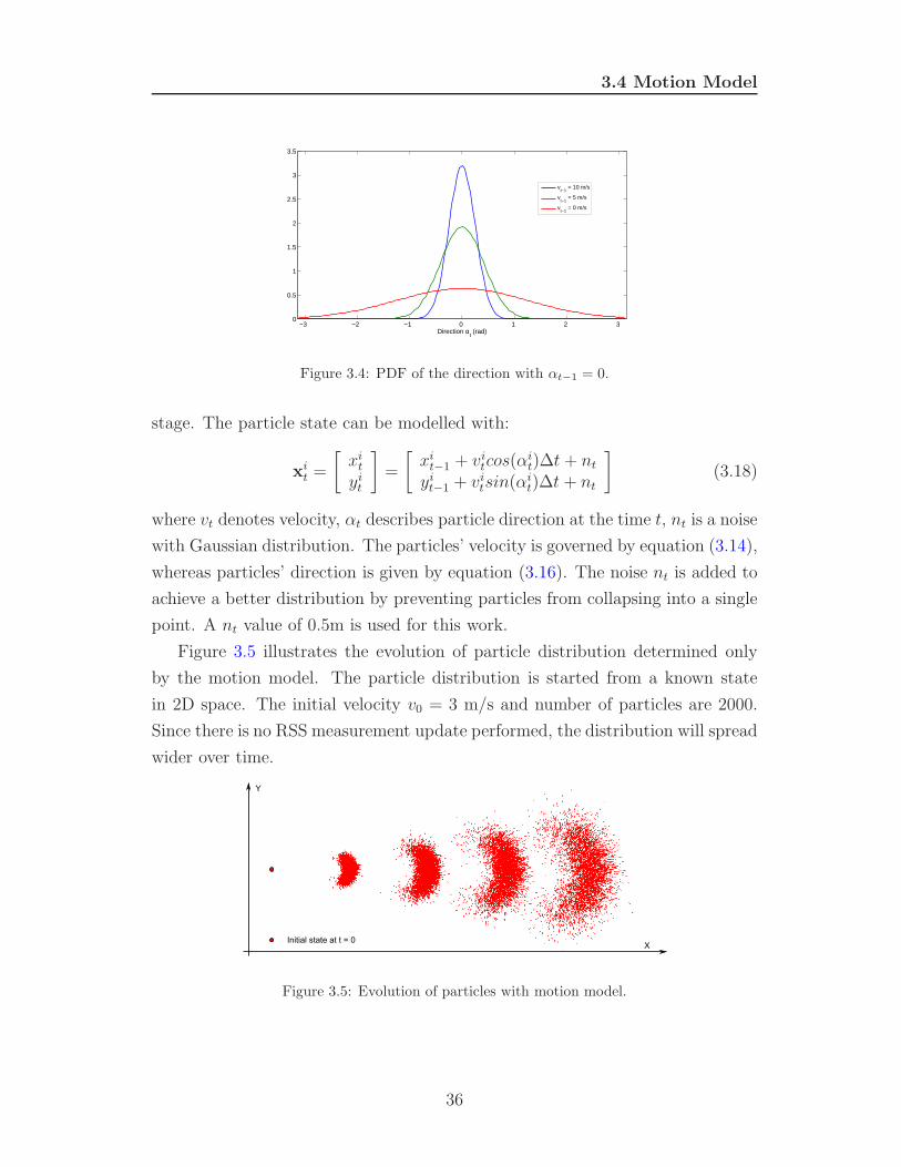
3.4 Motion Model
−3 −2 −1 0 1 2 3 0
0.5
1
1.5
2
2.5
3
3.5
Direction αt (rad)
vt−1
= 10 m/s
vt−1
= 5 m/s
vt−1
= 0 m/s
Figure 3.4: PDF of the direction with αt−1 = 0.
stage. The particle state can be modelled with:
xit =
[
xit
yit
]
=
[
xit−1 + vi
tcos(αit)∆t + nt
yit−1 + vi
tsin(αit)∆t + nt
]
(3.18)
where vt denotes velocity, αt describes particle direction at the time t, nt is a noise
with Gaussian distribution. The particles’ velocity is governed by equation (3.14),
whereas particles’ direction is given by equation (3.16). The noise nt is added to
achieve a better distribution by preventing particles from collapsing into a single
point. A nt value of 0.5m is used for this work.
Figure 3.5 illustrates the evolution of particle distribution determined only
by the motion model. The particle distribution is started from a known state
in 2D space. The initial velocity v0 = 3 m/s and number of particles are 2000.
Since there is no RSS measurement update performed, the distribution will spread
wider over time.
Figure 3.5: Evolution of particles with motion model.
36
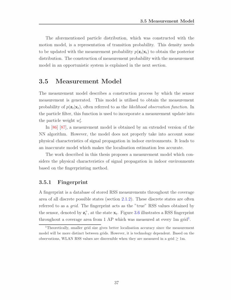
3.5 Measurement Model
The aforementioned particle distribution, which was constructed with the
motion model, is a representation of transition probability. This density needs
to be updated with the measurement probability p(zt|xt) to obtain the posterior
distribution. The construction of measurement probability with the measurement
model in an opportunistic system is explained in the next section.
3.5 Measurement Model
The measurement model describes a construction process by which the sensor
measurement is generated. This model is utilised to obtain the measurement
probability of p(zt|xt), often referred to as the likelihood observation function. In
the particle filter, this function is used to incorporate a measurement update into
the particle weight wit.
In [86] [87], a measurement model is obtained by an extended version of the
NN algorithm. However, the model does not properly take into account some
physical characteristics of signal propagation in indoor environments. It leads to
an inaccurate model which makes the localisation estimation less accurate.
The work described in this thesis proposes a measurement model which con-
siders the physical characteristics of signal propagation in indoor environments
based on the fingerprinting method.
3.5.1 Fingerprint
A fingerprint is a database of stored RSS measurements throughout the coverage
area of all discrete possible states (section 2.1.2). These discrete states are often
referred to as a grid. The fingerprint acts as the ”true” RSS values obtained by
the sensor, denoted by z+t , at the state xt. Figure 3.6 illustrates a RSS fingerprint
throughout a coverage area from 1 AP which was measured at every 1m grid1.
1Theoretically, smaller grid size gives better localisation accuracy since the measurement
model will be more distinct between grids. However, it is technology dependent. Based on the
observations, WLAN RSS values are discernible when they are measured in a grid ≥ 1m.
37
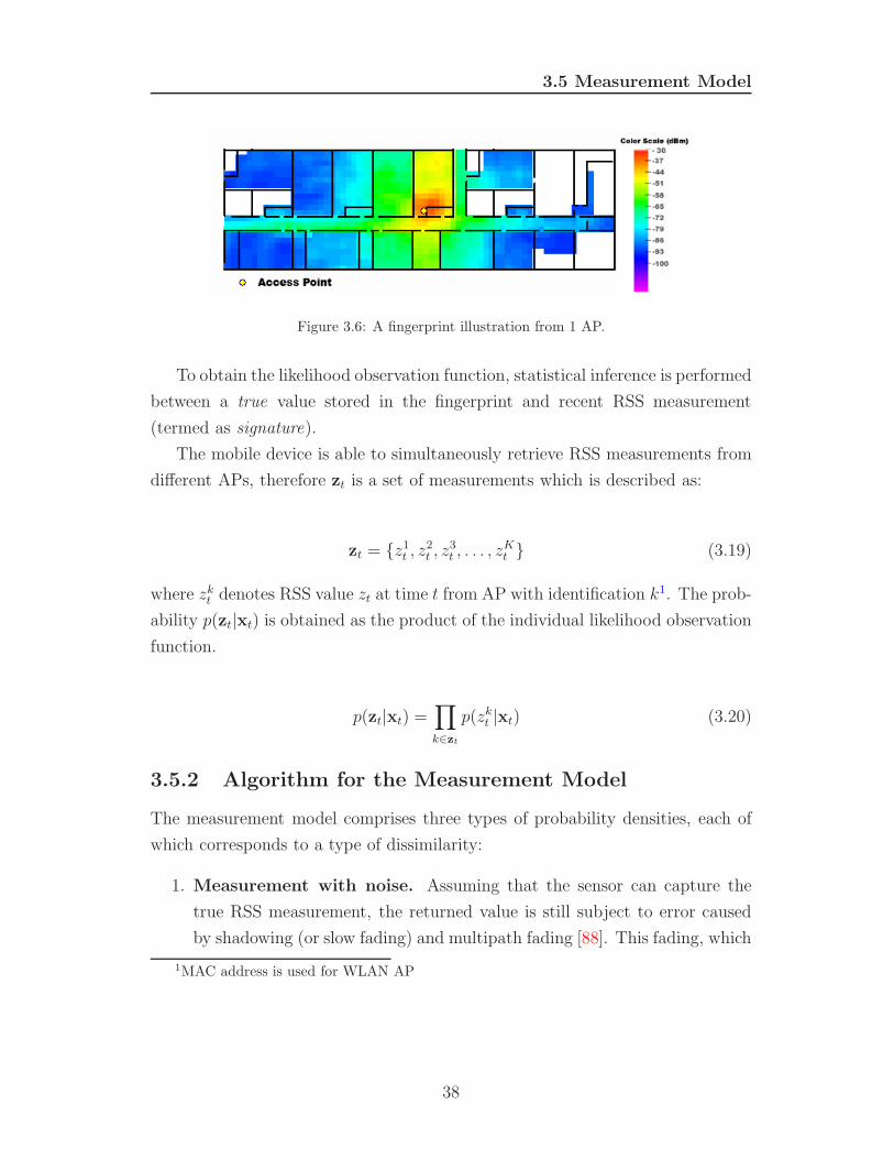
3.5 Measurement Model
Figure 3.6: A fingerprint illustration from 1 AP.
To obtain the likelihood observation function, statistical inference is performed
between a true value stored in the fingerprint and recent RSS measurement
(termed as signature).
The mobile device is able to simultaneously retrieve RSS measurements from
different APs, therefore zt is a set of measurements which is described as:
zt = {z1t , z
2t , z
3t , . . . , z
Kt } (3.19)
where zkt denotes RSS value zt at time t from AP with identification k1. The prob-
ability p(zt|xt) is obtained as the product of the individual likelihood observation
function.
p(zt|xt) =∏
k∈zt
p(zkt |xt) (3.20)
3.5.2 Algorithm for the Measurement Model
The measurement model comprises three types of probability densities, each of
which corresponds to a type of dissimilarity:
1. Measurement with noise. Assuming that the sensor can capture the
true RSS measurement, the returned value is still subject to error caused
by shadowing (or slow fading) and multipath fading [88]. This fading, which
1MAC address is used for WLAN AP
38
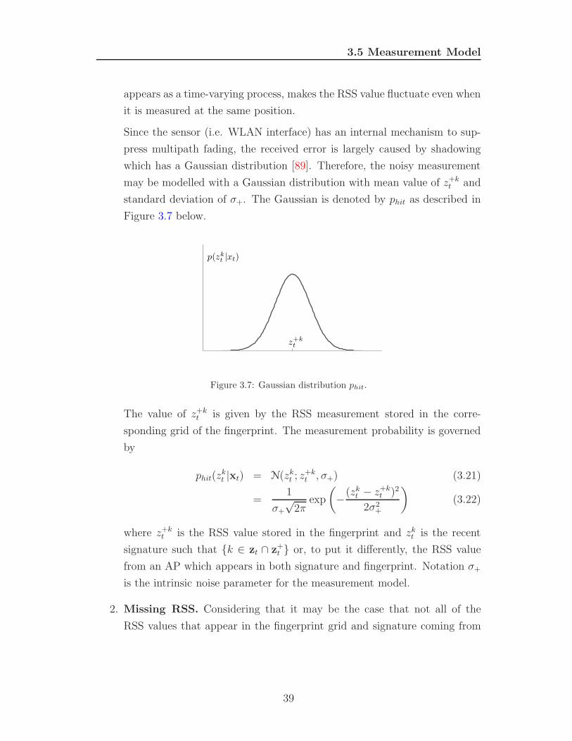
3.5 Measurement Model
appears as a time-varying process, makes the RSS value fluctuate even when
it is measured at the same position.
Since the sensor (i.e. WLAN interface) has an internal mechanism to sup-
press multipath fading, the received error is largely caused by shadowing
which has a Gaussian distribution [89]. Therefore, the noisy measurement
may be modelled with a Gaussian distribution with mean value of z+kt and
standard deviation of σ+. The Gaussian is denoted by phit as described in
Figure 3.7 below.
z+k
t
p(zkt|xt)
Figure 3.7: Gaussian distribution phit.
The value of z+kt is given by the RSS measurement stored in the corre-
sponding grid of the fingerprint. The measurement probability is governed
by
phit(zkt |xt) = N(zk
t ; z+kt , σ+) (3.21)
=1
σ+
√2π
exp
(
−(zkt − z+k
t )2
2σ2+
)
(3.22)
where z+kt is the RSS value stored in the fingerprint and zk
t is the recent
signature such that {k ∈ zt ∩ z+t } or, to put it differently, the RSS value
from an AP which appears in both signature and fingerprint. Notation σ+
is the intrinsic noise parameter for the measurement model.
2. Missing RSS. Considering that it may be the case that not all of the
RSS values that appear in the fingerprint grid and signature coming from
39
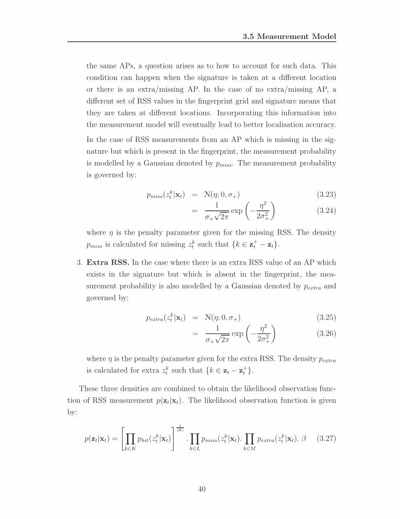
3.5 Measurement Model
the same APs, a question arises as to how to account for such data. This
condition can happen when the signature is taken at a different location
or there is an extra/missing AP. In the case of no extra/missing AP, a
different set of RSS values in the fingerprint grid and signature means that
they are taken at different locations. Incorporating this information into
the measurement model will eventually lead to better localisation accuracy.
In the case of RSS measurements from an AP which is missing in the sig-
nature but which is present in the fingerprint, the measurement probability
is modelled by a Gaussian denoted by pmiss. The measurement probability
is governed by:
pmiss(zkt |xt) = N(η; 0, σ+) (3.23)
=1
σ+
√2π
exp
(
− η2
2σ2+
)
(3.24)
where η is the penalty parameter given for the missing RSS. The density
pmiss is calculated for missing zkt such that {k ∈ z+
t − zt}.
3. Extra RSS. In the case where there is an extra RSS value of an AP which
exists in the signature but which is absent in the fingerprint, the mea-
surement probability is also modelled by a Gaussian denoted by pextra and
governed by:
pextra(zkt |xt) = N(η; 0, σ+) (3.25)
=1
σ+
√2π
exp
(
− η2
2σ2+
)
(3.26)
where η is the penalty parameter given for the extra RSS. The density pextra
is calculated for extra zkt such that {k ∈ zt − z+
t }.
These three densities are combined to obtain the likelihood observation func-
tion of RSS measurement p(zt|xt). The likelihood observation function is given
by:
p(zt|xt) =
[
∏
k∈K
phit(zkt |xt)
]1
|K|
.∏
k∈L
pmiss(zkt |xt).
∏
k∈M
pextra(zkt |xt). β (3.27)
40
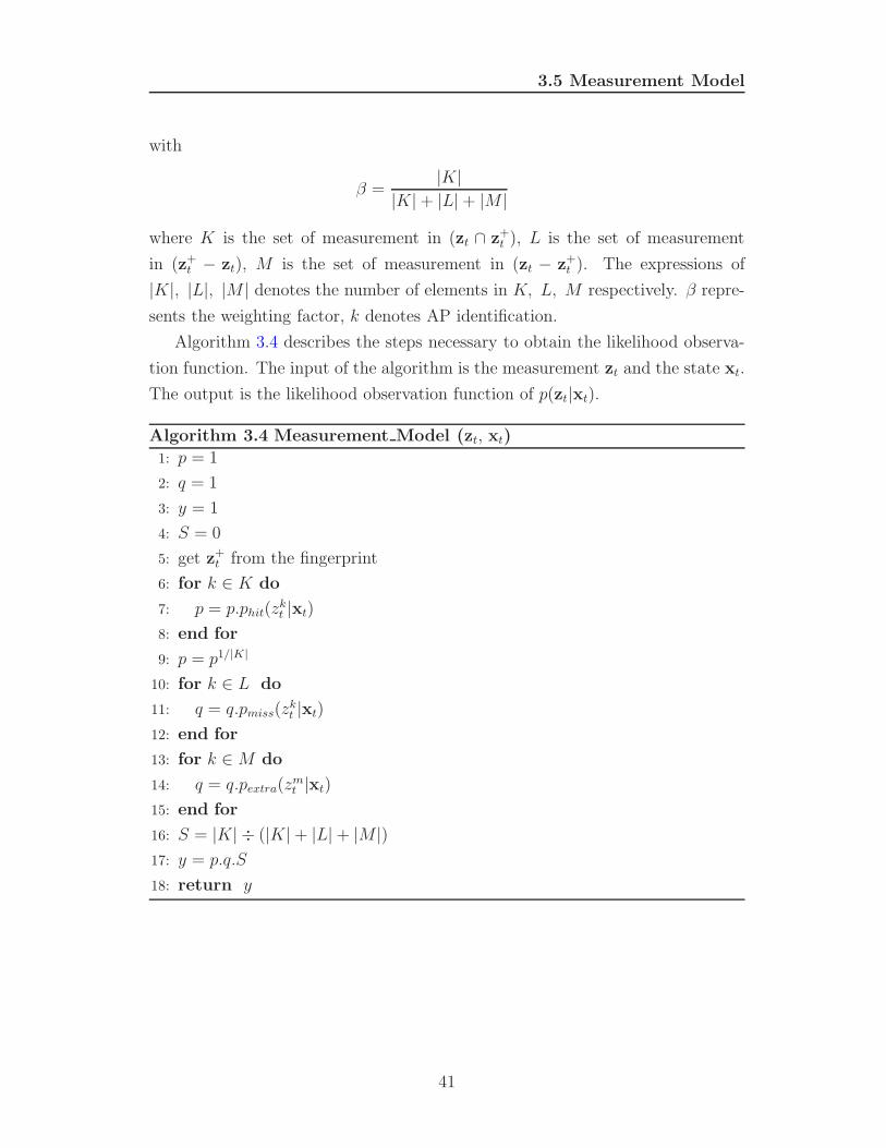
3.5 Measurement Model
with
β =|K|
|K| + |L| + |M |
where K is the set of measurement in (zt ∩ z+t ), L is the set of measurement
in (z+t − zt), M is the set of measurement in (zt − z+
t ). The expressions of
|K|, |L|, |M | denotes the number of elements in K, L, M respectively. β repre-
sents the weighting factor, k denotes AP identification.
Algorithm 3.4 describes the steps necessary to obtain the likelihood observa-
tion function. The input of the algorithm is the measurement zt and the state xt.
The output is the likelihood observation function of p(zt|xt).
Algorithm 3.4 Measurement Model (zt, xt)
1: p = 1
2: q = 1
3: y = 1
4: S = 0
5: get z+t from the fingerprint
6: for k ∈ K do
7: p = p.phit(zkt |xt)
8: end for
9: p = p1/|K|
10: for k ∈ L do
11: q = q.pmiss(zkt |xt)
12: end for
13: for k ∈ M do
14: q = q.pextra(zmt |xt)
15: end for
16: S = |K| ÷ (|K| + |L| + |M |)17: y = p.q.S
18: return y
41
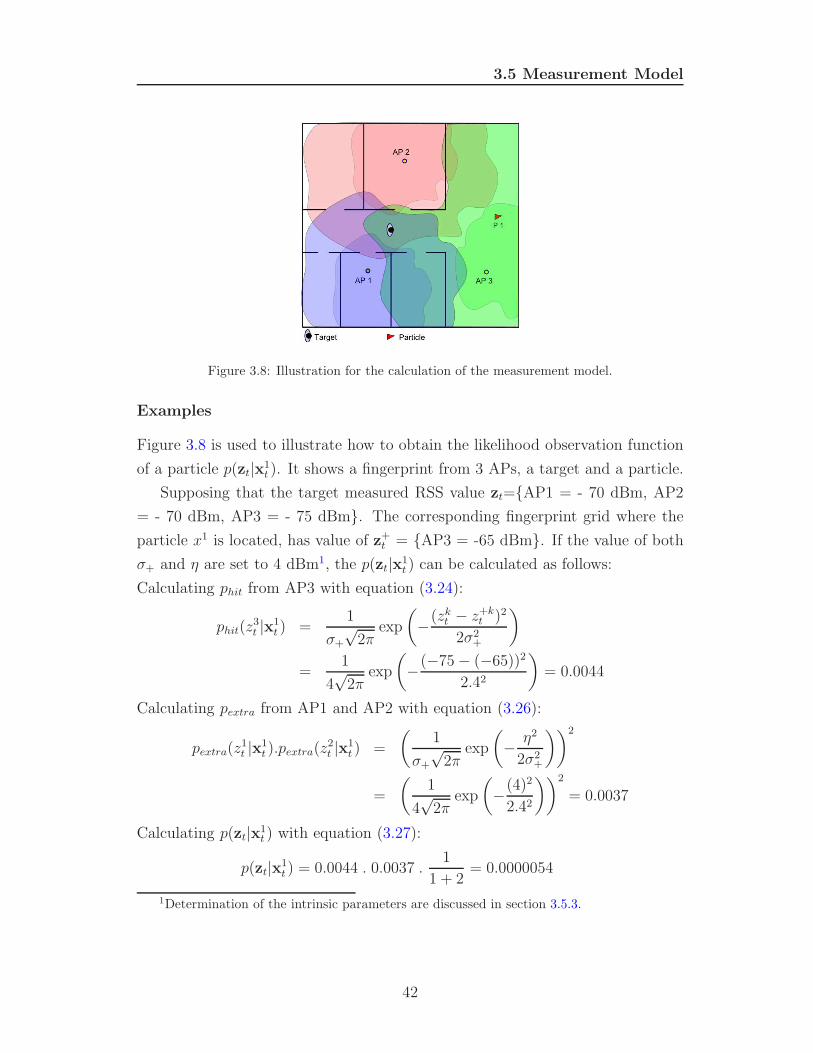
3.5 Measurement Model
Figure 3.8: Illustration for the calculation of the measurement model.
Examples
Figure 3.8 is used to illustrate how to obtain the likelihood observation function
of a particle p(zt|x1t ). It shows a fingerprint from 3 APs, a target and a particle.
Supposing that the target measured RSS value zt={AP1 = - 70 dBm, AP2
= - 70 dBm, AP3 = - 75 dBm}. The corresponding fingerprint grid where the
particle x1 is located, has value of z+t = {AP3 = -65 dBm}. If the value of both
σ+ and η are set to 4 dBm1, the p(zt|x1t ) can be calculated as follows:
Calculating phit from AP3 with equation (3.24):
phit(z3t |x1
t ) =1
σ+
√2π
exp
(
−(zkt − z+k
t )2
2σ2+
)
=1
4√
2πexp
(
−(−75 − (−65))2
2.42
)
= 0.0044
Calculating pextra from AP1 and AP2 with equation (3.26):
pextra(z1t |x1
t ).pextra(z2t |x1
t ) =
(
1
σ+
√2π
exp
(
− η2
2σ2+
))2
=
(
1
4√
2πexp
(
−(4)2
2.42
))2
= 0.0037
Calculating p(zt|x1t ) with equation (3.27):
p(zt|x1t ) = 0.0044 . 0.0037 .
1
1 + 2= 0.0000054
1Determination of the intrinsic parameters are discussed in section 3.5.3.
42
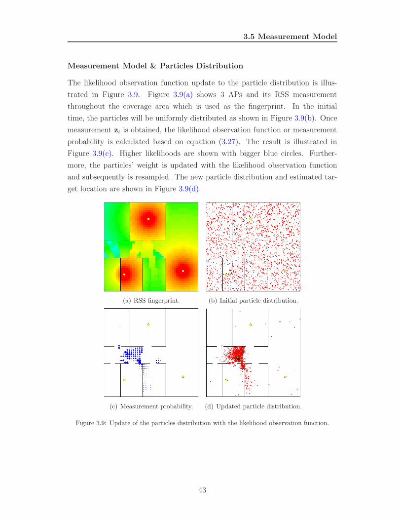
3.5 Measurement Model
Measurement Model & Particles Distribution
The likelihood observation function update to the particle distribution is illus-
trated in Figure 3.9. Figure 3.9(a) shows 3 APs and its RSS measurement
throughout the coverage area which is used as the fingerprint. In the initial
time, the particles will be uniformly distributed as shown in Figure 3.9(b). Once
measurement zt is obtained, the likelihood observation function or measurement
probability is calculated based on equation (3.27). The result is illustrated in
Figure 3.9(c). Higher likelihoods are shown with bigger blue circles. Further-
more, the particles’ weight is updated with the likelihood observation function
and subsequently is resampled. The new particle distribution and estimated tar-
get location are shown in Figure 3.9(d).
(a) RSS fingerprint. (b) Initial particle distribution.
(c) Measurement probability. (d) Updated particle distribution.
Figure 3.9: Update of the particles distribution with the likelihood observation function.
43
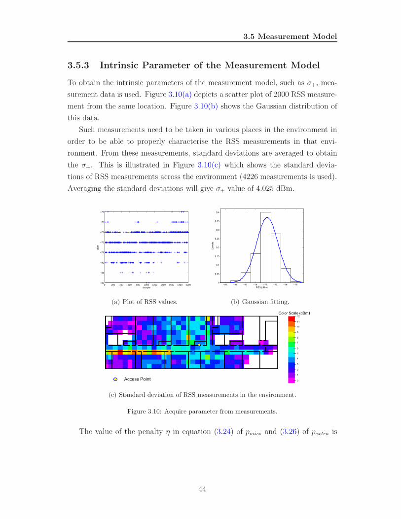
3.5 Measurement Model
3.5.3 Intrinsic Parameter of the Measurement Model
To obtain the intrinsic parameters of the measurement model, such as σ+, mea-
surement data is used. Figure 3.10(a) depicts a scatter plot of 2000 RSS measure-
ment from the same location. Figure 3.10(b) shows the Gaussian distribution of
this data.
Such measurements need to be taken in various places in the environment in
order to be able to properly characterise the RSS measurements in that envi-
ronment. From these measurements, standard deviations are averaged to obtain
the σ+. This is illustrated in Figure 3.10(c) which shows the standard devia-
tions of RSS measurements across the environment (4226 measurements is used).
Averaging the standard deviations will give σ+ value of 4.025 dBm.
0 200 400 600 800 1000 1200 1400 1600 1800 2000−82
−81
−80
−79
−78
−77
−76
−75
Sample
dBm
(a) Plot of RSS values.
−82 −81 −80 −79 −78 −77 −76 −750
0.05
0.1
0.15
0.2
0.25
0.3
0.35
0.4
RSS (dBm)
Den
sity
(b) Gaussian fitting.
(c) Standard deviation of RSS measurements in the environment.
Figure 3.10: Acquire parameter from measurements.
The value of the penalty η in equation (3.24) of pmiss and (3.26) of pextra is
44
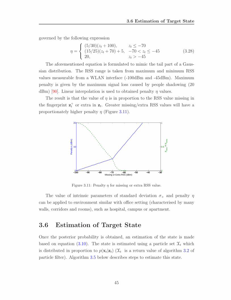
3.6 Estimation of Target State
governed by the following expression
η =
(5/30)(zt + 100), zt ≤ −70(15/25)(zt + 70) + 5, −70 < zt ≤ −4520, zt > −45
(3.28)
The aforementioned equation is formulated to mimic the tail part of a Gaus-
sian distribution. The RSS range is taken from maximum and minimum RSS
values measurable from a WLAN interface (-100dBm and -45dBm). Maximum
penalty is given by the maximum signal loss caused by people shadowing (20
dBm) [90]. Linear interpolation is used to obtained penalty η values.
The result is that the value of η is in proportion to the RSS value missing in
the fingerprint z+t or extra in zt. Greater missing/extra RSS values will have a
proportionately higher penalty η (Figure 3.11).
−100 −90 −80 −70 −60 −50 −40 −300
10
20
Pen
alty
η (
dBm
)
−100 −90 −80 −70 −60 −50 −40 −300
0.5
1
Missing or Extra RSS (dBm)
p mis
s or
p extr
a
Figure 3.11: Penalty η for missing or extra RSS value.
The value of intrinsic parameters of standard deviation σ+ and penalty η
can be applied to environment similar with office setting (characterised by many
walls, corridors and rooms), such as hospital, campus or apartment.
3.6 Estimation of Target State
Once the posterior probability is obtained, an estimation of the state is made
based on equation (3.10). The state is estimated using a particle set Xt which
is distributed in proportion to p(xt|zt) (Xt is a return value of algorithm 3.2 of
particle filter). Algorithm 3.5 below describes steps to estimate this state.
45
3.7 Conclusion
Algorithm 3.5 State Estimation(Xt)
1: xt = 0
2: for i = 1 to |Xt| do
3: xt = xt + xit.w
it
4: end for
5: return xt
3.7 Conclusion
This chapter described the implementation of a particle filter algorithm to im-
prove the accuracy of opportunistic indoor localisation. The ability to deal with
a non-linear and non-Gaussian system, the suitability for estimation of dynamic
state with large process noise, and the robustness of the algorithm make the
particle filter an ideal approach for RSS-based opportunistic system.
Furthermore, motion and measurement models were devised to enable the
implementation of particle filter into opportunistic system. The approach for the
motion model is a combination of the Brownian movement and the first-order
motion model. This approach is novel and more accurately reflects the target’s
kinematics behaviour in opportunistic system. The proposed measurement model
properly considers the physical characteristics of signal propagation in indoor
environments. It leads to more accurate model which in turn leads to more
accurate location estimation.
The implementation of a particle filter in an opportunistic system through
the invention of measurement and motion models is novel and become one of the
research contributions.
To improve further the accuracy of opportunistic indoor localisation, this re-
search looks at other information beyond the available signal in the environment.
This research also advances current approaches in fingerprinting to significantly
enhance the usability of the system.
The collection of algorithms to further increase the accuracy and usability
of the opportunistic system is the next contribution of the research and will be
described in the following chapter.
46
Chapter 4
Learning Data Fusion
The previous chapter presented the implementation of the particle filter to in-
crease the accuracy of opportunistic indoor localisation. It was achieved through
the application of novel measurement and motion models.
To further improve the accuracy, this research examines other information
beyond the available signal in the environment, i.e. map information and particle
trajectory. The fusion1 of extra information, in addition to RSS measurement, is
the distinct characteristic of the algorithms explained in this chapter.
Filtering particle motion with map information is used to further increase the
accuracy of opportunistic system (section 4.1). Moreover, particle trajectory is
fused to refine state estimation with backtracking particle filter algorithm (sec-
tion 4.2).
Furthermore, the research advances current methods in fingerprinting to ad-
dress the usability problem (section 4.3). The novelty of the algorithm lies in
the ability to automatically build and maintain the fingerprint up-to-date, thus
significantly enhancing the usability of the opportunistic indoor localisation.
The collection of algorithm presented in this chapter is one of the most im-
portant contributions of this research.
1See section 2.2.2 for the definition of data fusion.
47
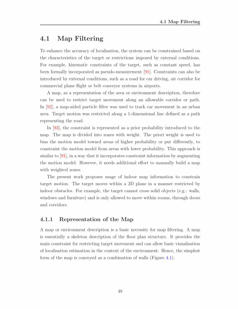
4.1 Map Filtering
4.1 Map Filtering
To enhance the accuracy of localisation, the system can be constrained based on
the characteristics of the target or restrictions imposed by external conditions.
For example, kinematic constraints of the target, such as constant speed, has
been formally incorporated as pseudo-measurement [91]. Constraints can also be
introduced by external conditions, such as a road for car driving, air corridor for
commercial plane flight or belt conveyor systems in airports.
A map, as a representation of the area or environment description, therefore
can be used to restrict target movement along an allowable corridor or path.
In [92], a map-aided particle filter was used to track car movement in an urban
area. Target motion was restricted along a 1-dimensional line defined as a path
representing the road.
In [93], the constraint is represented as a prior probability introduced to the
map. The map is divided into zones with weight. The priori weight is used to
bias the motion model toward areas of higher probability or put differently, to
constraint the motion model from areas with lower probability. This approach is
similar to [91], in a way that it incorporates constraint information by augmenting
the motion model. However, it needs additional effort to manually build a map
with weighted zones.
The present work proposes usage of indoor map information to constrain
target motion. The target moves within a 2D plane in a manner restricted by
indoor obstacles. For example, the target cannot cross solid objects (e.g.: walls,
windows and furniture) and is only allowed to move within rooms, through doors
and corridors.
4.1.1 Representation of the Map
A map or environment description is a basic necessity for map filtering. A map
is essentially a skeleton description of the floor plan structure. It provides the
main constraint for restricting target movement and can allow basic visualisation
of localisation estimation in the context of the environment. Hence, the simplest
form of the map is conveyed as a combination of walls (Figure 4.1).
48
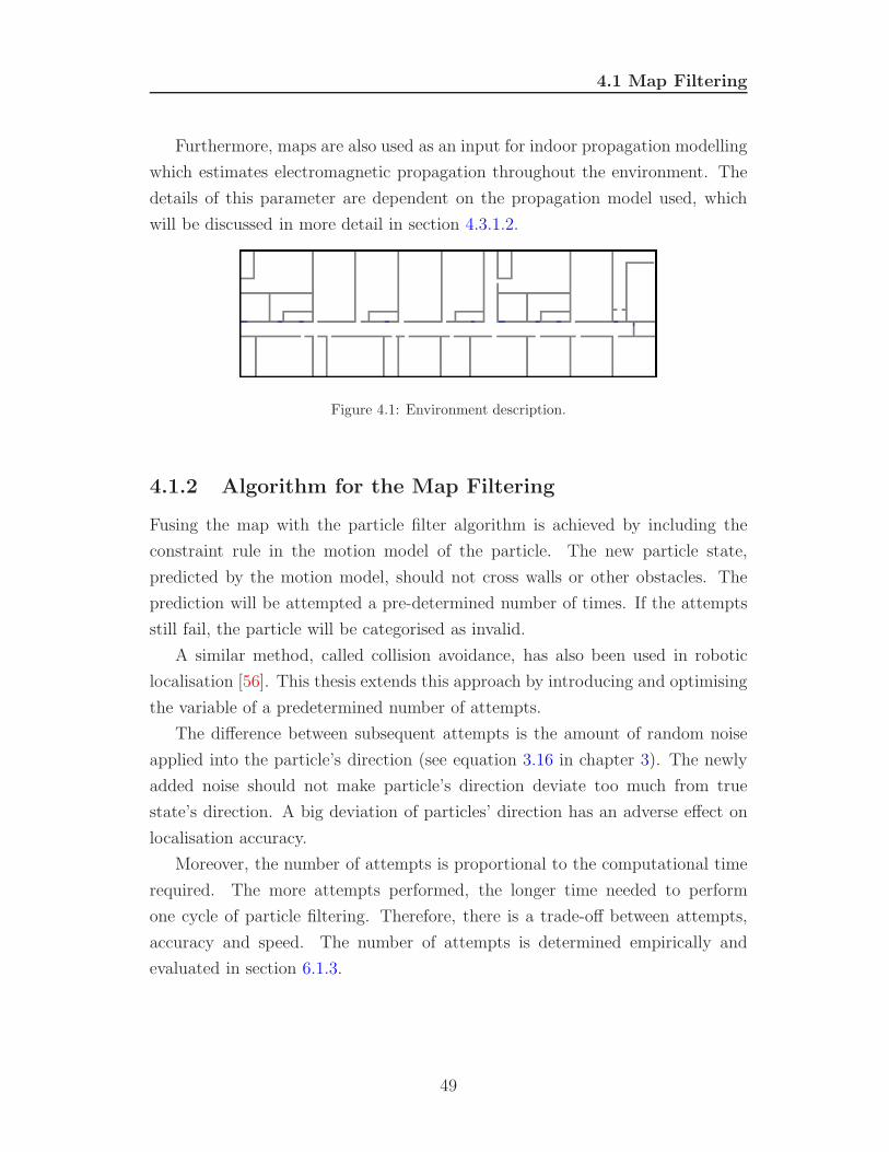
4.1 Map Filtering
Furthermore, maps are also used as an input for indoor propagation modelling
which estimates electromagnetic propagation throughout the environment. The
details of this parameter are dependent on the propagation model used, which
will be discussed in more detail in section 4.3.1.2.
Figure 4.1: Environment description.
4.1.2 Algorithm for the Map Filtering
Fusing the map with the particle filter algorithm is achieved by including the
constraint rule in the motion model of the particle. The new particle state,
predicted by the motion model, should not cross walls or other obstacles. The
prediction will be attempted a pre-determined number of times. If the attempts
still fail, the particle will be categorised as invalid.
A similar method, called collision avoidance, has also been used in robotic
localisation [56]. This thesis extends this approach by introducing and optimising
the variable of a predetermined number of attempts.
The difference between subsequent attempts is the amount of random noise
applied into the particle’s direction (see equation 3.16 in chapter 3). The newly
added noise should not make particle’s direction deviate too much from true
state’s direction. A big deviation of particles’ direction has an adverse effect on
localisation accuracy.
Moreover, the number of attempts is proportional to the computational time
required. The more attempts performed, the longer time needed to perform
one cycle of particle filtering. Therefore, there is a trade-off between attempts,
accuracy and speed. The number of attempts is determined empirically and
evaluated in section 6.1.3.
49
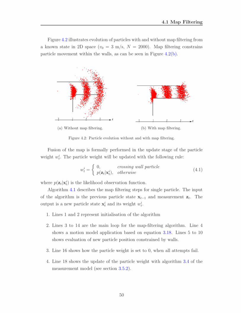
4.1 Map Filtering
Figure 4.2 illustrates evolution of particles with and without map filtering from
a known state in 2D space (v0 = 3 m/s, N = 2000). Map filtering constrains
particle movement within the walls, as can be seen in Figure 4.2(b).
(a) Without map filtering. (b) With map filtering.
Figure 4.2: Particle evolution without and with map filtering.
Fusion of the map is formally performed in the update stage of the particle
weight wit. The particle weight will be updated with the following rule:
wit =
{
0, crossing wall particlep(zt|xi
t), otherwise(4.1)
where p(zt|xit) is the likelihood observation function.
Algorithm 4.1 describes the map filtering steps for single particle. The input
of the algorithm is the previous particle state xt−1 and measurement zt. The
output is a new particle state xit and its weight wi
t.
1. Lines 1 and 2 represent initialisation of the algorithm
2. Lines 3 to 14 are the main loop for the map-filtering algorithm. Line 4
shows a motion model application based on equation 3.18. Lines 5 to 10
shows evaluation of new particle position constrained by walls.
3. Line 16 shows how the particle weight is set to 0, when all attempts fail.
4. Line 18 shows the update of the particle weight with algorithm 3.4 of the
measurement model (see section 3.5.2).
50

4.2 Backtracking Particle Filter
5. Line 20 shows the algorithm return, i.e. current particle state with its
associated weight.
Algorithm 4.1 MapFiltering (xit−1, zt)
1: A = number of attempts
2: c = false
3: for a = 1 to A do
4: given xit−1, predict the particle state xi
t {with the motion model}5: for j = 1 to number of wall do
6: c = particle state xit cross the wallj
7: if c = true then
8: break
9: end if
10: end for
11: if c = false then
12: break
13: end if
14: end for
15: if c = true then
16: wit = 0
17: else
18: wit = p(zt|xt
i) {given by the measurement model}19: end if
20: return xit, wi
t
4.2 Backtracking Particle Filter
Fusing map information to increase the accuracy of the opportunistic system has
been proposed in the previous section. Information that can be fused to further
increase the accuracy is particle trajectory1.
Backtracking particle filter (BPF) is a technique for refining state estimates
based on particle trajectory. Incorporation of the map filtering technique allows
1Trajectory is set of time-ordered states representing the path taken by each particle
51
4.2 Backtracking Particle Filter
the BPF to exploit the long-range geometrical constraints of a map1 and a long-
term likelihood observation function.
If some particles xt are not valid at some time t, the previous state estimates
back to b time steps xt−b can be refined by removing the invalid particle trajec-
tories. This is based on the assumption that an invalid particle is the result of
a particle that follows an invalid trajectory or path. Therefore, recalculation of
the previous state estimation xt−b without invalid trajectories will produce bet-
ter estimates. In order to enable backtracking, each particle has to remember its
state history or trajectory.
BPF implementation for opportunistic localisation is illustrated in the follow-
ing figures. Figure 4.3(a) shows a typical phenomenon when a standard particle
filter is used for opportunistic localisation. It shows the posterior density of the
particles at four time-steps. The position estimates and the ground truth are
shown in the diagram as well.
A particle deemed to be invalid when it is filtered out by the map filtering
technique or by the likelihood function (performed in the 3rd time-step). For
instance, a crossing wall particle will be categorised as invalid by map filtering
technique and its weight is set to zero. A particle is also deemed as invalid
if its weight, given by likelihood function, is very low. The invalid particles
subsequently are not resampled in the 4th time-step.
Figure 4.3(b) shows how the BPF removes the invalid trajectories. Fig-
ure 4.3(c) illustrates the recalculation of the state estimation after backtracking.
It is evident that, under certain conditions, BPF can improve the state estimation
relative to a normal PF. This condition will be evaluated in section 6.1.3.
Algorithm 4.2 describes the steps necessary for BPF:
1. Line 1 refers to the increment of counter B, which shows how many esti-
mations have been made.
2. Line 2 refers to the prediction stage of particle with the motion model.
During the prediction stage, a new particle is sampled from the transition
density p(xt|xt−1) with the map filtering technique. The new particle xt will
save the previous state xt−1.
1A wall used to filter current particle state xit
can affect previous states.
52
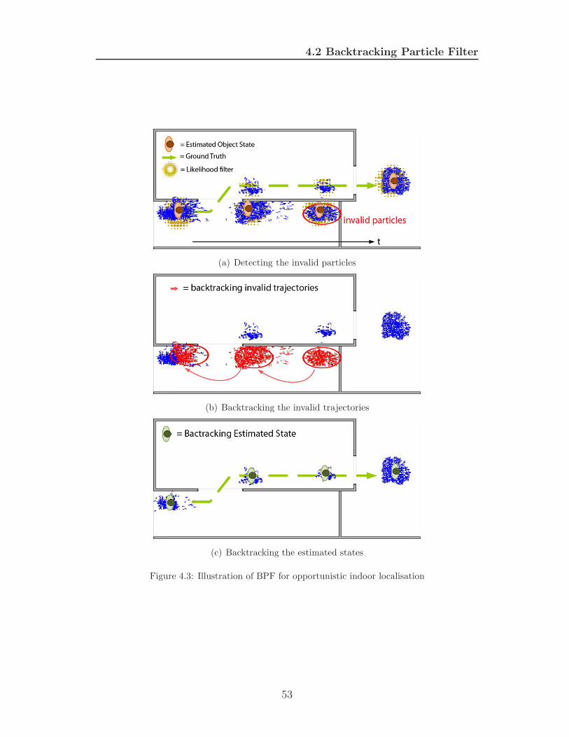
4.2 Backtracking Particle Filter
(a) Detecting the invalid particles
(b) Backtracking the invalid trajectories
(c) Backtracking the estimated states
Figure 4.3: Illustration of BPF for opportunistic indoor localisation
53
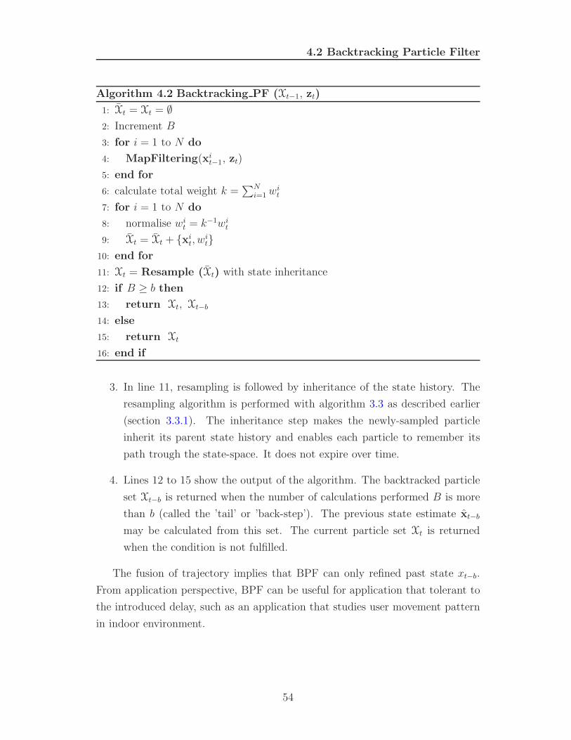
4.2 Backtracking Particle Filter
Algorithm 4.2 Backtracking PF (Xt−1, zt)
1: Xt = Xt = ∅2: Increment B
3: for i = 1 to N do
4: MapFiltering(xit−1, zt)
5: end for
6: calculate total weight k =∑N
i=1 wit
7: for i = 1 to N do
8: normalise wit = k−1wi
t
9: Xt = Xt + {xit, w
it}
10: end for
11: Xt = Resample (Xt) with state inheritance
12: if B ≥ b then
13: return Xt, Xt−b
14: else
15: return Xt
16: end if
3. In line 11, resampling is followed by inheritance of the state history. The
resampling algorithm is performed with algorithm 3.3 as described earlier
(section 3.3.1). The inheritance step makes the newly-sampled particle
inherit its parent state history and enables each particle to remember its
path trough the state-space. It does not expire over time.
4. Lines 12 to 15 show the output of the algorithm. The backtracked particle
set Xt−b is returned when the number of calculations performed B is more
than b (called the ’tail’ or ’back-step’). The previous state estimate xt−b
may be calculated from this set. The current particle set Xt is returned
when the condition is not fulfilled.
The fusion of trajectory implies that BPF can only refined past state xt−b.
From application perspective, BPF can be useful for application that tolerant to
the introduced delay, such as an application that studies user movement pattern
in indoor environment.
54
4.3 Self-Calibration Fingerprinting
4.2.1 Summary
Fusing map information to increase the accuracy of the opportunistic system had
been proposed with the map filtering technique. Information that can be fused
to further increase the accuracy is particle trajectory.
The fusion of particle trajectory is performed with the BPF algorithm. BPF
is a technique for refining state estimates based on particle trajectory histories.
This is based on the assumption that an invalid particle is the result of a particle
that follows an invalid trajectory or path. Therefore, recalculation of the previous
state estimation without invalid trajectories will produce better estimates.
Furthermore, the trajectory concept is expanded further to advance current
fingerprinting methods. Set of hypothetical trajectories are proposed, evaluated
and weighted in self-calibration fingerprinting algorithm to address usability prob-
lem in opportunistic system. The following section will elaborate self-calibration
fingerprinting algorithm in detail.
4.3 Self-Calibration Fingerprinting
The objective of a self-calibration fingerprinting algorithm is to advance current
approaches in fingerprinting in order to address the usability problem of oppor-
tunistic system.
The self-calibration for the opportunistic system eliminates labour-intensive
and cumbersome manual calibration and makes the fingerprint adaptive to any
change in the system or environment configuration. The algorithm maintains the
fingerprint up-to-date, thus achieving self-calibration of the localisation system.
Self-calibration fingerprinting is one of the most important contributions of this
research.
The self-calibration fingerprint takes advantage of a fingerprint prediction
with propagation model. However, it enhances this further by automatically
re-calibrating parameters required for the propagation model across the environ-
ment and time. The algorithm learns from the history of measurement, target
movement pattern and map description to accurately adjust the parameter of the
propagation model.
55
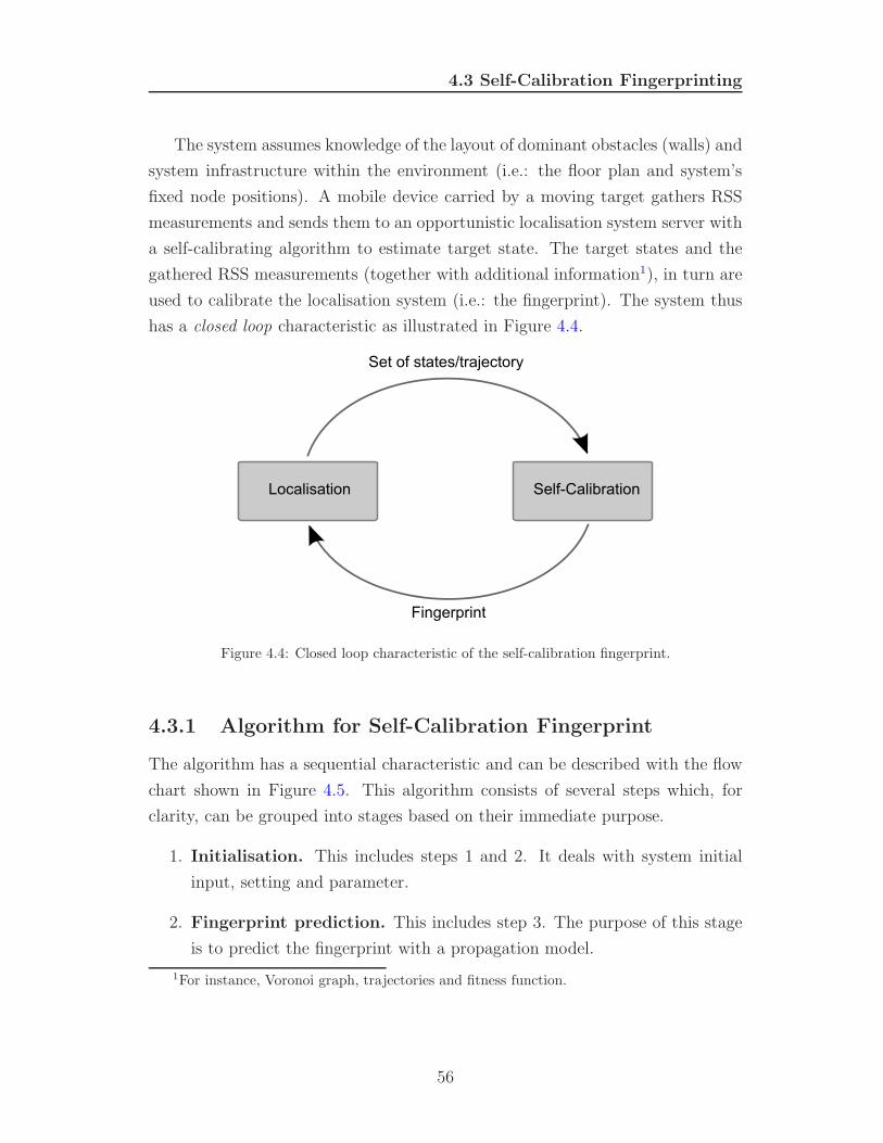
4.3 Self-Calibration Fingerprinting
The system assumes knowledge of the layout of dominant obstacles (walls) and
system infrastructure within the environment (i.e.: the floor plan and system’s
fixed node positions). A mobile device carried by a moving target gathers RSS
measurements and sends them to an opportunistic localisation system server with
a self-calibrating algorithm to estimate target state. The target states and the
gathered RSS measurements (together with additional information1), in turn are
used to calibrate the localisation system (i.e.: the fingerprint). The system thus
has a closed loop characteristic as illustrated in Figure 4.4.
Figure 4.4: Closed loop characteristic of the self-calibration fingerprint.
4.3.1 Algorithm for Self-Calibration Fingerprint
The algorithm has a sequential characteristic and can be described with the flow
chart shown in Figure 4.5. This algorithm consists of several steps which, for
clarity, can be grouped into stages based on their immediate purpose.
1. Initialisation. This includes steps 1 and 2. It deals with system initial
input, setting and parameter.
2. Fingerprint prediction. This includes step 3. The purpose of this stage
is to predict the fingerprint with a propagation model.
1For instance, Voronoi graph, trajectories and fitness function.
56
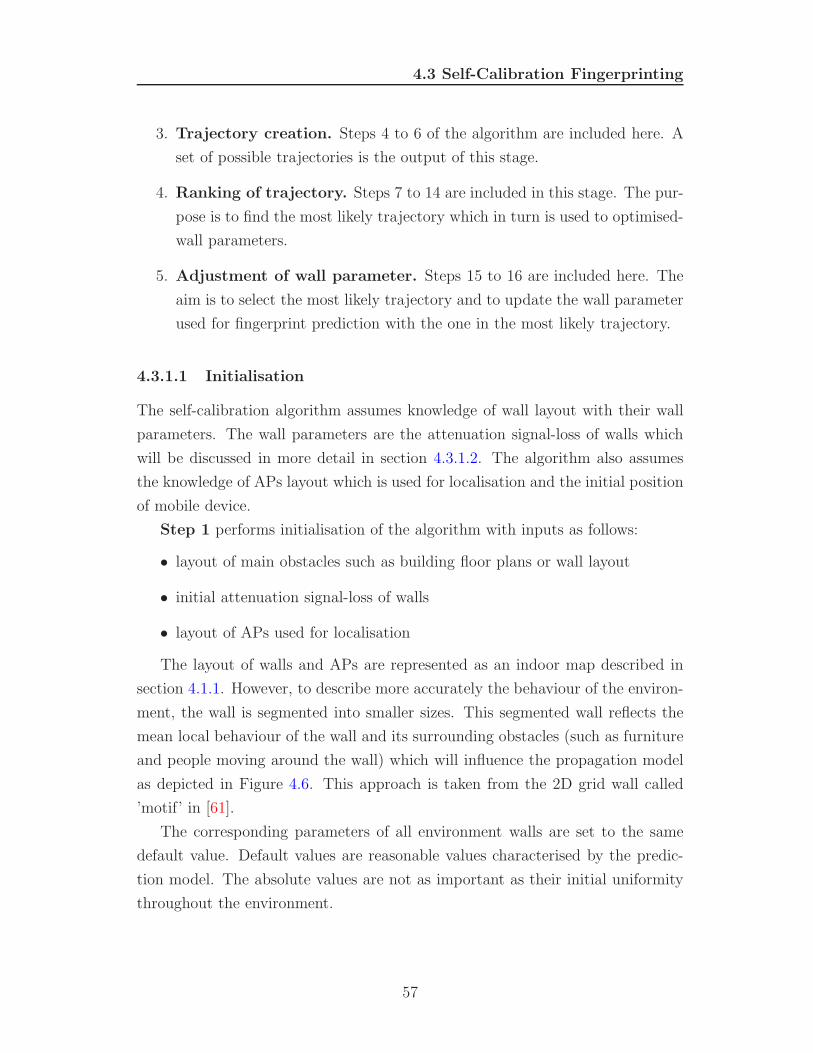
4.3 Self-Calibration Fingerprinting
3. Trajectory creation. Steps 4 to 6 of the algorithm are included here. A
set of possible trajectories is the output of this stage.
4. Ranking of trajectory. Steps 7 to 14 are included in this stage. The pur-
pose is to find the most likely trajectory which in turn is used to optimised-
wall parameters.
5. Adjustment of wall parameter. Steps 15 to 16 are included here. The
aim is to select the most likely trajectory and to update the wall parameter
used for fingerprint prediction with the one in the most likely trajectory.
4.3.1.1 Initialisation
The self-calibration algorithm assumes knowledge of wall layout with their wall
parameters. The wall parameters are the attenuation signal-loss of walls which
will be discussed in more detail in section 4.3.1.2. The algorithm also assumes
the knowledge of APs layout which is used for localisation and the initial position
of mobile device.
Step 1 performs initialisation of the algorithm with inputs as follows:
• layout of main obstacles such as building floor plans or wall layout
• initial attenuation signal-loss of walls
• layout of APs used for localisation
The layout of walls and APs are represented as an indoor map described in
section 4.1.1. However, to describe more accurately the behaviour of the environ-
ment, the wall is segmented into smaller sizes. This segmented wall reflects the
mean local behaviour of the wall and its surrounding obstacles (such as furniture
and people moving around the wall) which will influence the propagation model
as depicted in Figure 4.6. This approach is taken from the 2D grid wall called
’motif’ in [61].
The corresponding parameters of all environment walls are set to the same
default value. Default values are reasonable values characterised by the predic-
tion model. The absolute values are not as important as their initial uniformity
throughout the environment.
57
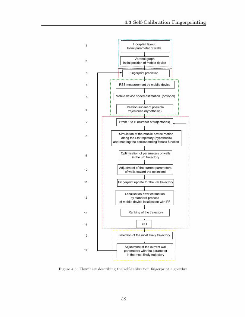
4.3 Self-Calibration Fingerprinting
Figure 4.5: Flowchart describing the self-calibration fingerprint algorithm.
58
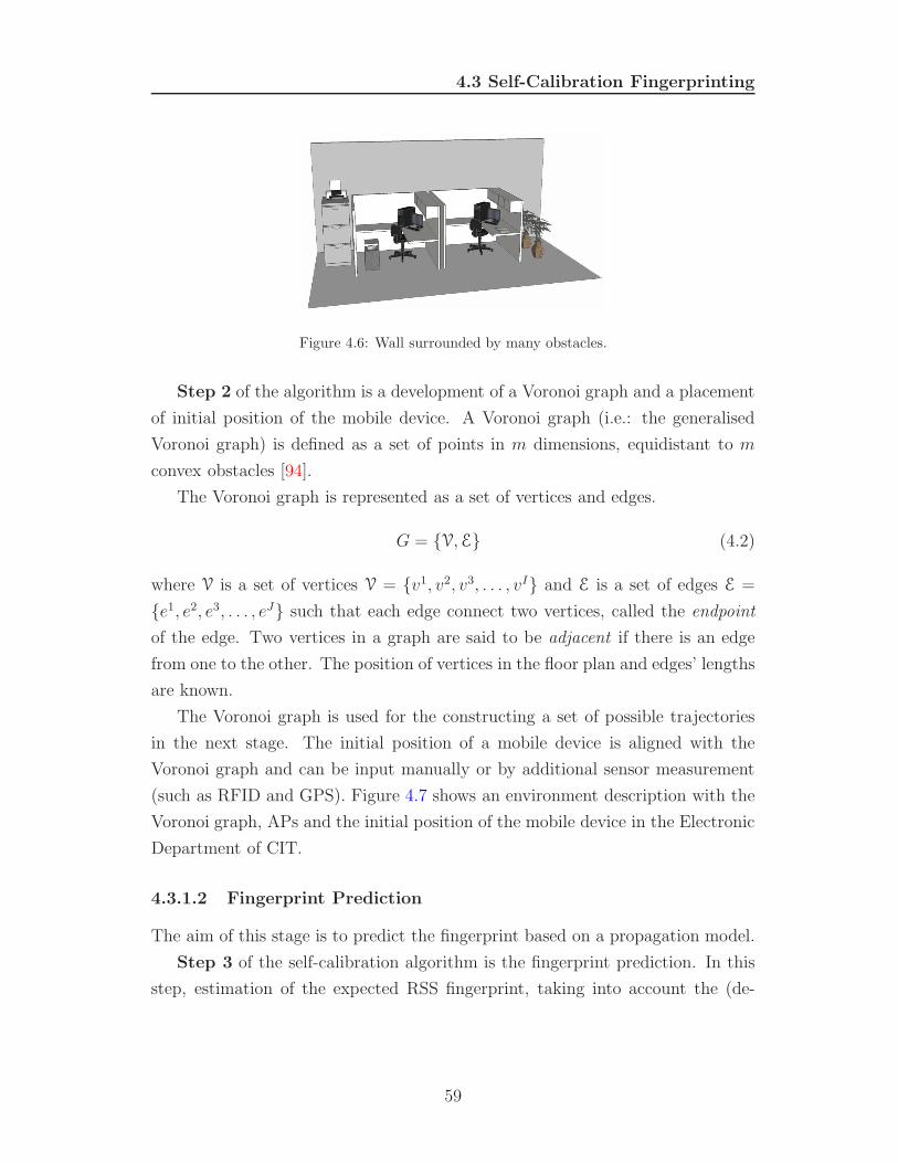
4.3 Self-Calibration Fingerprinting
Figure 4.6: Wall surrounded by many obstacles.
Step 2 of the algorithm is a development of a Voronoi graph and a placement
of initial position of the mobile device. A Voronoi graph (i.e.: the generalised
Voronoi graph) is defined as a set of points in m dimensions, equidistant to m
convex obstacles [94].
The Voronoi graph is represented as a set of vertices and edges.
G = {V, E} (4.2)
where V is a set of vertices V = {v1, v2, v3, . . . , vI} and E is a set of edges E =
{e1, e2, e3, . . . , eJ} such that each edge connect two vertices, called the endpoint
of the edge. Two vertices in a graph are said to be adjacent if there is an edge
from one to the other. The position of vertices in the floor plan and edges’ lengths
are known.
The Voronoi graph is used for the constructing a set of possible trajectories
in the next stage. The initial position of a mobile device is aligned with the
Voronoi graph and can be input manually or by additional sensor measurement
(such as RFID and GPS). Figure 4.7 shows an environment description with the
Voronoi graph, APs and the initial position of the mobile device in the Electronic
Department of CIT.
4.3.1.2 Fingerprint Prediction
The aim of this stage is to predict the fingerprint based on a propagation model.
Step 3 of the self-calibration algorithm is the fingerprint prediction. In this
step, estimation of the expected RSS fingerprint, taking into account the (de-
59
4.3 Self-Calibration Fingerprinting
Figure 4.7: Map with Voronoi graph, APs and initial position of mobile device.
fault) parameters of the wall, is performed by appropriate empirical or physical
propagation models.
A simple empirical approach, the MWM, is utilised for fingerprint prediction.
MWM is chosen because of its simplicity and fast propagation prediction. Fur-
thermore, it allows the application of linear optimisation (section 4.3.1.4). These
factors contribute to the speed of overall algorithm, which is important factor for
increasing the usability of opportunistic system.
In the MWM, the path loss is given by the following equation [95]:
L = L1 + 20 log(d) + Lw + Lf (4.3)
where
Lw =
I∑
i=1
Lwi =
I∑
i=1
aiwki
w (4.4)
Lf = afkf (4.5)
L denotes the predicted signal loss, L1 is the free space loss at a distance of 1 m
from the transmitter, d is the distance from the transmitter to the receiver, Lw
is the contribution of walls to the total signal loss, Lf is the contribution of floors
to the total signal loss. Lwi denotes the contribution of wall of ith type to the
total signal loss, aiw denotes the transmission loss factor of one wall of ith type,
kiw denotes the number of walls of ith type, I is the number of wall types, af is
the transmission loss factor of one floor, kf is the number of floors.
This model takes into account the loss factor of wall and floor depending on
their thickness and material composition. Figure 4.8 shows fingerprint prediction
60
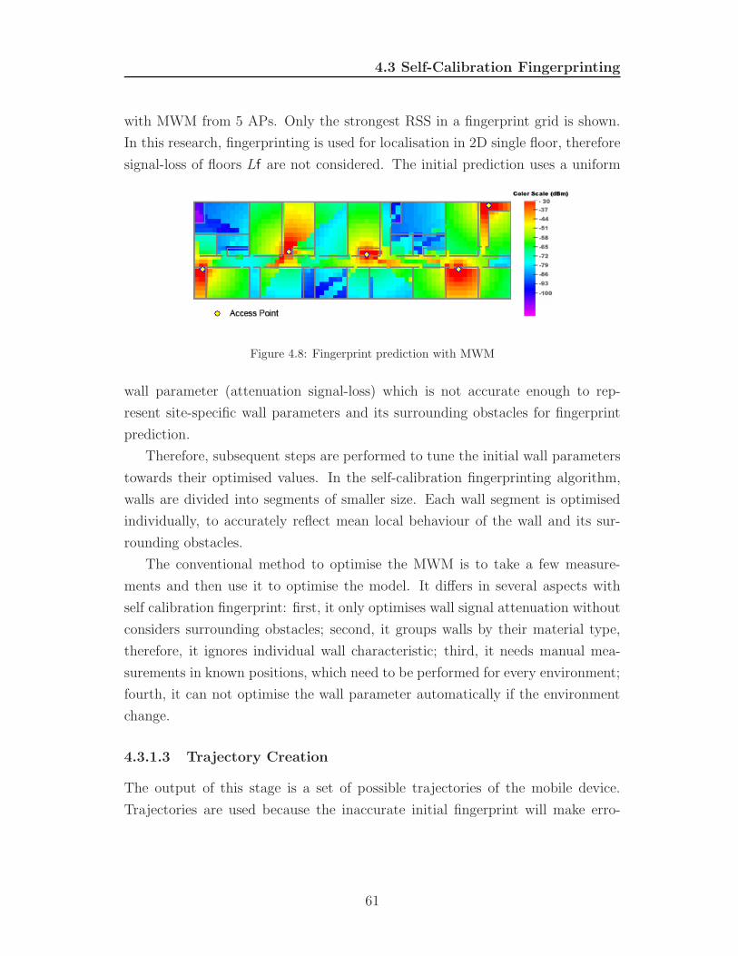
4.3 Self-Calibration Fingerprinting
with MWM from 5 APs. Only the strongest RSS in a fingerprint grid is shown.
In this research, fingerprinting is used for localisation in 2D single floor, therefore
signal-loss of floors Lf are not considered. The initial prediction uses a uniform
Figure 4.8: Fingerprint prediction with MWM
wall parameter (attenuation signal-loss) which is not accurate enough to rep-
resent site-specific wall parameters and its surrounding obstacles for fingerprint
prediction.
Therefore, subsequent steps are performed to tune the initial wall parameters
towards their optimised values. In the self-calibration fingerprinting algorithm,
walls are divided into segments of smaller size. Each wall segment is optimised
individually, to accurately reflect mean local behaviour of the wall and its sur-
rounding obstacles.
The conventional method to optimise the MWM is to take a few measure-
ments and then use it to optimise the model. It differs in several aspects with
self calibration fingerprint: first, it only optimises wall signal attenuation without
considers surrounding obstacles; second, it groups walls by their material type,
therefore, it ignores individual wall characteristic; third, it needs manual mea-
surements in known positions, which need to be performed for every environment;
fourth, it can not optimise the wall parameter automatically if the environment
change.
4.3.1.3 Trajectory Creation
The output of this stage is a set of possible trajectories of the mobile device.
Trajectories are used because the inaccurate initial fingerprint will make erro-
61
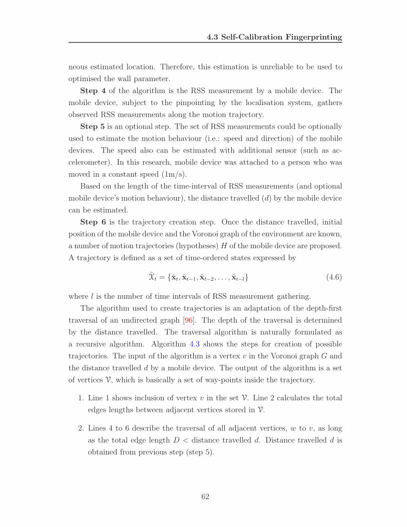
4.3 Self-Calibration Fingerprinting
neous estimated location. Therefore, this estimation is unreliable to be used to
optimised the wall parameter.
Step 4 of the algorithm is the RSS measurement by a mobile device. The
mobile device, subject to the pinpointing by the localisation system, gathers
observed RSS measurements along the motion trajectory.
Step 5 is an optional step. The set of RSS measurements could be optionally
used to estimate the motion behaviour (i.e.: speed and direction) of the mobile
devices. The speed also can be estimated with additional sensor (such as ac-
celerometer). In this research, mobile device was attached to a person who was
moved in a constant speed (1m/s).
Based on the length of the time-interval of RSS measurements (and optional
mobile device’s motion behaviour), the distance travelled (d) by the mobile device
can be estimated.
Step 6 is the trajectory creation step. Once the distance travelled, initial
position of the mobile device and the Voronoi graph of the environment are known,
a number of motion trajectories (hypotheses) H of the mobile device are proposed.
A trajectory is defined as a set of time-ordered states expressed by
Xt = {xt, xt−1, xt−2, . . . , xt−l} (4.6)
where l is the number of time intervals of RSS measurement gathering.
The algorithm used to create trajectories is an adaptation of the depth-first
traversal of an undirected graph [96]. The depth of the traversal is determined
by the distance travelled. The traversal algorithm is naturally formulated as
a recursive algorithm. Algorithm 4.3 shows the steps for creation of possible
trajectories. The input of the algorithm is a vertex v in the Voronoi graph G and
the distance travelled d by a mobile device. The output of the algorithm is a set
of vertices V, which is basically a set of way-points inside the trajectory.
1. Line 1 shows inclusion of vertex v in the set V. Line 2 calculates the total
edges lengths between adjacent vertices stored in V.
2. Lines 4 to 6 describe the traversal of all adjacent vertices, w to v, as long
as the total edge length D < distance travelled d. Distance travelled d is
obtained from previous step (step 5).
62
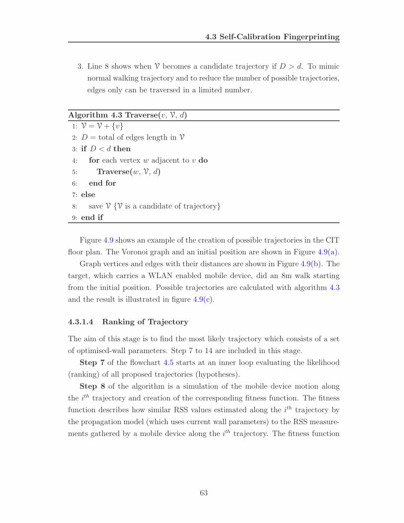
4.3 Self-Calibration Fingerprinting
3. Line 8 shows when V becomes a candidate trajectory if D > d. To mimic
normal walking trajectory and to reduce the number of possible trajectories,
edges only can be traversed in a limited number.
Algorithm 4.3 Traverse(v, V, d)
1: V = V + {v}2: D = total of edges length in V
3: if D < d then
4: for each vertex w adjacent to v do
5: Traverse(w, V, d)
6: end for
7: else
8: save V {V is a candidate of trajectory}9: end if
Figure 4.9 shows an example of the creation of possible trajectories in the CIT
floor plan. The Voronoi graph and an initial position are shown in Figure 4.9(a).
Graph vertices and edges with their distances are shown in Figure 4.9(b). The
target, which carries a WLAN enabled mobile device, did an 8m walk starting
from the initial position. Possible trajectories are calculated with algorithm 4.3
and the result is illustrated in figure 4.9(c).
4.3.1.4 Ranking of Trajectory
The aim of this stage is to find the most likely trajectory which consists of a set
of optimised-wall parameters. Step 7 to 14 are included in this stage.
Step 7 of the flowchart 4.5 starts at an inner loop evaluating the likelihood
(ranking) of all proposed trajectories (hypotheses).
Step 8 of the algorithm is a simulation of the mobile device motion along
the ith trajectory and creation of the corresponding fitness function. The fitness
function describes how similar RSS values estimated along the ith trajectory by
the propagation model (which uses current wall parameters) to the RSS measure-
ments gathered by a mobile device along the ith trajectory. The fitness function
63
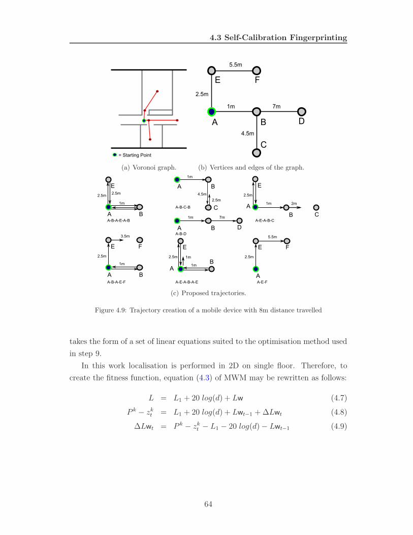
4.3 Self-Calibration Fingerprinting
(a) Voronoi graph. (b) Vertices and edges of the graph.
(c) Proposed trajectories.
Figure 4.9: Trajectory creation of a mobile device with 8m distance travelled
takes the form of a set of linear equations suited to the optimisation method used
in step 9.
In this work localisation is performed in 2D on single floor. Therefore, to
create the fitness function, equation (4.3) of MWM may be rewritten as follows:
L = L1 + 20 log(d) + Lw (4.7)
P k − zkt = L1 + 20 log(d) + Lwt−1 + ∆Lwt (4.8)
∆Lwt = P k − zkt − L1 − 20 log(d) − Lwt−1 (4.9)
64
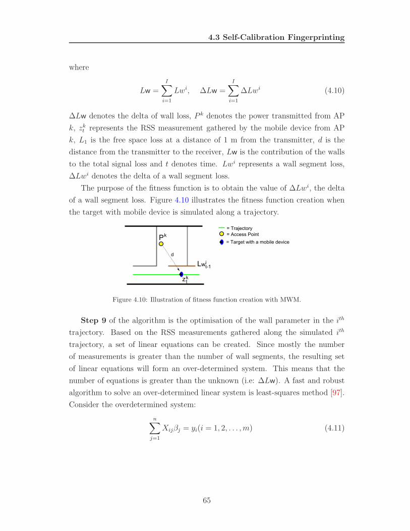
4.3 Self-Calibration Fingerprinting
where
Lw =
I∑
i=1
Lwi, ∆Lw =
I∑
i=1
∆Lwi (4.10)
∆Lw denotes the delta of wall loss, P k denotes the power transmitted from AP
k, zkt represents the RSS measurement gathered by the mobile device from AP
k, L1 is the free space loss at a distance of 1 m from the transmitter, d is the
distance from the transmitter to the receiver, Lw is the contribution of the walls
to the total signal loss and t denotes time. Lwi represents a wall segment loss,
∆Lwi denotes the delta of a wall segment loss.
The purpose of the fitness function is to obtain the value of ∆Lwi, the delta
of a wall segment loss. Figure 4.10 illustrates the fitness function creation when
the target with mobile device is simulated along a trajectory.
Figure 4.10: Illustration of fitness function creation with MWM.
Step 9 of the algorithm is the optimisation of the wall parameter in the ith
trajectory. Based on the RSS measurements gathered along the simulated ith
trajectory, a set of linear equations can be created. Since mostly the number
of measurements is greater than the number of wall segments, the resulting set
of linear equations will form an over-determined system. This means that the
number of equations is greater than the unknown (i.e: ∆Lw). A fast and robust
algorithm to solve an over-determined linear system is least-squares method [97].
Consider the overdetermined system:
n∑
j=1
Xijβj = yi(i = 1, 2, . . . , m) (4.11)
65
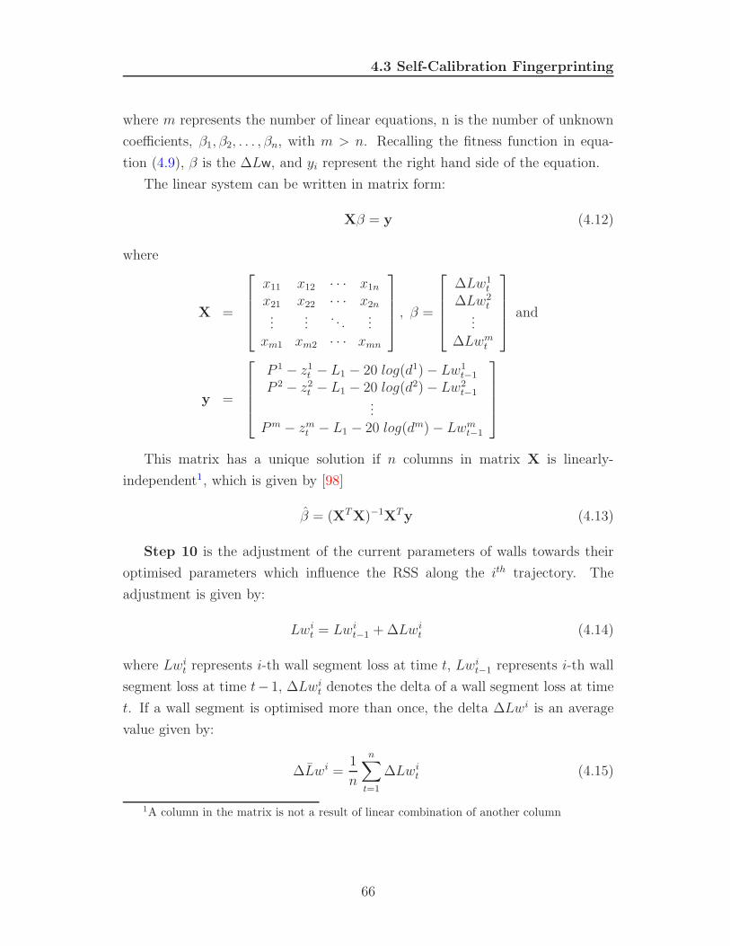
4.3 Self-Calibration Fingerprinting
where m represents the number of linear equations, n is the number of unknown
coefficients, β1, β2, . . . , βn, with m > n. Recalling the fitness function in equa-
tion (4.9), β is the ∆Lw, and yi represent the right hand side of the equation.
The linear system can be written in matrix form:
Xβ = y (4.12)
where
X =
x11 x12 · · · x1n
x21 x22 · · · x2n...
.... . .
...xm1 xm2 · · · xmn
, β =
∆Lw1t
∆Lw2t
...∆Lwm
t
and
y =
P 1 − z1t − L1 − 20 log(d1) − Lw1
t−1
P 2 − z2t − L1 − 20 log(d2) − Lw2
t−1...
P m − zmt − L1 − 20 log(dm) − Lwm
t−1
This matrix has a unique solution if n columns in matrix X is linearly-
independent1, which is given by [98]
β = (XTX)−1XTy (4.13)
Step 10 is the adjustment of the current parameters of walls towards their
optimised parameters which influence the RSS along the ith trajectory. The
adjustment is given by:
Lwit = Lwi
t−1 + ∆Lwit (4.14)
where Lwit represents i-th wall segment loss at time t, Lwi
t−1 represents i-th wall
segment loss at time t− 1, ∆Lwit denotes the delta of a wall segment loss at time
t. If a wall segment is optimised more than once, the delta ∆Lwi is an average
value given by:
∆Lwi =1
n
n∑
t=1
∆Lwit (4.15)
1A column in the matrix is not a result of linear combination of another column
66
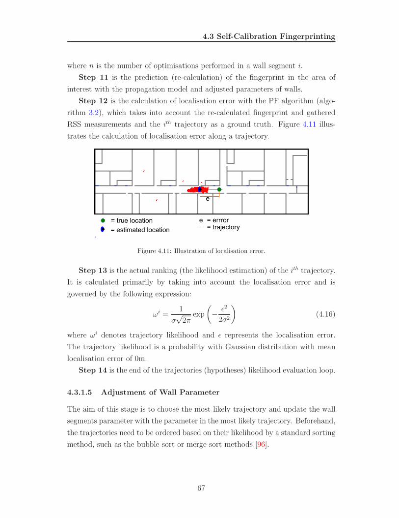
4.3 Self-Calibration Fingerprinting
where n is the number of optimisations performed in a wall segment i.
Step 11 is the prediction (re-calculation) of the fingerprint in the area of
interest with the propagation model and adjusted parameters of walls.
Step 12 is the calculation of localisation error with the PF algorithm (algo-
rithm 3.2), which takes into account the re-calculated fingerprint and gathered
RSS measurements and the ith trajectory as a ground truth. Figure 4.11 illus-
trates the calculation of localisation error along a trajectory.
Figure 4.11: Illustration of localisation error.
Step 13 is the actual ranking (the likelihood estimation) of the ith trajectory.
It is calculated primarily by taking into account the localisation error and is
governed by the following expression:
ωi =1
σ√
2πexp
(
− ε2
2σ2
)
(4.16)
where ωi denotes trajectory likelihood and ε represents the localisation error.
The trajectory likelihood is a probability with Gaussian distribution with mean
localisation error of 0m.
Step 14 is the end of the trajectories (hypotheses) likelihood evaluation loop.
4.3.1.5 Adjustment of Wall Parameter
The aim of this stage is to choose the most likely trajectory and update the wall
segments parameter with the parameter in the most likely trajectory. Beforehand,
the trajectories need to be ordered based on their likelihood by a standard sorting
method, such as the bubble sort or merge sort methods [96].
67
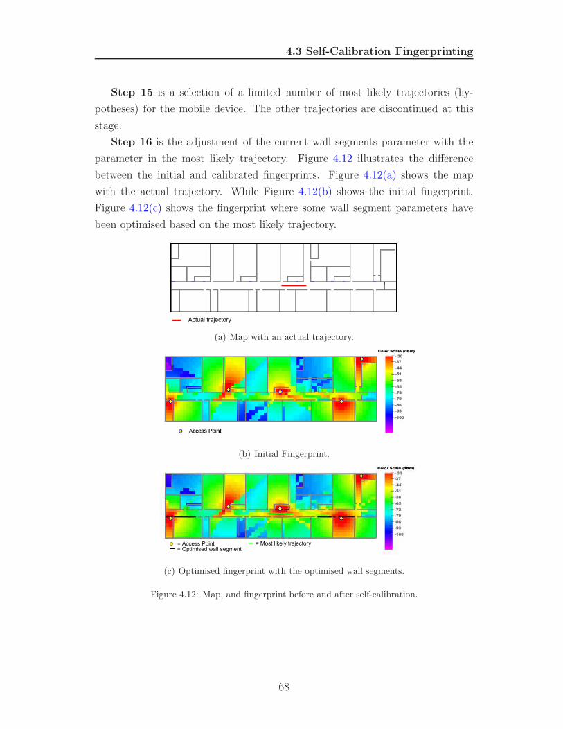
4.3 Self-Calibration Fingerprinting
Step 15 is a selection of a limited number of most likely trajectories (hy-
potheses) for the mobile device. The other trajectories are discontinued at this
stage.
Step 16 is the adjustment of the current wall segments parameter with the
parameter in the most likely trajectory. Figure 4.12 illustrates the difference
between the initial and calibrated fingerprints. Figure 4.12(a) shows the map
with the actual trajectory. While Figure 4.12(b) shows the initial fingerprint,
Figure 4.12(c) shows the fingerprint where some wall segment parameters have
been optimised based on the most likely trajectory.
(a) Map with an actual trajectory.
(b) Initial Fingerprint.
(c) Optimised fingerprint with the optimised wall segments.
Figure 4.12: Map, and fingerprint before and after self-calibration.
68
4.4 Conclusion
4.4 Conclusion
This chapter described the fusion of map information, particle trajectory and
RSS measurement. The fusion is performed to further improve the accuracy of
opportunistic system.
Map information is used to constrain particle motion with the map filtering
algorithm. Fusing the map with the particle filter algorithm is achieved by in-
cluding the constraint rule in the motion model of the particle. The new particle
state, predicted by the motion model, should not cross walls or other obstacles.
Furthermore, the fusion of particle trajectory is performed with BPF algo-
rithm. BPF is a technique for refining state estimates based on particle tra-
jectory histories. Recalculation of the previous state estimation without invalid
trajectories will produce better estimation.
The development of map filtering and backtracking particle filter in oppor-
tunistic system is novel contribution of this research.
Furthermore, this chapter presented an advancement of current fingerprinting
methods with the self-calibration algorithm. The objective of the self-calibration
fingerprinting algorithm is to significantly enhance the usability of an opportunis-
tic system.
The self-calibration algorithm combines several advanced techniques, such as
an indoor propagation model, Voronoi graph, graph traversal, trajectory concept,
linear optimisation with least-square method and a particle filter. This algorithm
advances state-of-the-art fingerprinting methods in several key areas: it removes
the necessity to collect initial training data; it elevates the necessity to place
dedicated RF receivers used for constantly measuring RSS values; it automatically
optimises wall parameter for the propagation model.
Using single type of measured phenomenon may not offer required accuracy,
but they can be fused with other sensor measurements to achieve better accu-
racy. The particle filter algorithm is used to fuse different sensory data when
more fine-grained accuracy is desirable or when required for different application
domains. The next chapter will describe the particle filter-based sensor data
fusion to increase the accuracy of indoor localisation system.
69
Chapter 5
Multi Sensor Data Fusion
The data fusion algorithm presented in the previous chapter fuses RSS mea-
surement, map information and particle trajectory to improve the accuracy of
opportunistic indoor localisation. However, using a single type of measured phe-
nomenon may not offer sufficient accuracy required for a particular application
domain. Fusion with different localisation technologies is needed to enhance the
accuracy of the opportunistic system.
Sensor data fusion1 described in this chapter is conducted in the context of
the Wearit@Work project2. The project investigated indoor localisation systems
required in an industrial setting (car factory) and fire-fighter scenario.
Fusion of WSN and WLAN is investigated to achieve more fine-grained ac-
curacy in an industrial setting (section 5.1). Furthermore, fusion of PDR, ul-
trasound and WSN is investigated for indoor localisation for fire-fighters (sec-
tion 5.2). The fusion of an opportunistic system with different technologies is a
novel approach and one of the contributions of this research.
To enable the implementation of particle filter-based fusion, motion models
and measurement models for different measured phenomenon have to be devised.
The novelty of the algorithm lies in the invented probabilistic models and will be
further described in the following sections.
1See section 2.2.2 for the definition of data fusion.2www.wearitatwork.com
70
5.1 Fusion of WSN and WLAN
5.1 Fusion of WSN and WLAN
WSN based on the IEEE 802.15.4 standard [99], are intended principally for
monitoring and control applications that demand very low power consumption
from a battery source. The range of coverage of a WSN node in indoor use is
typically 10-20m.
Based on the standard, a WSN node provides a measured value, called link
quality indication (LQI), which can be used for localisation purposes. The LQI
can be implemented as RSS, signal-to-noise ratio or a combination of the two.
The LQI of WSN is received for each message data-packet and is the result of
averaging over eight symbols [9]. Furthermore, a WSN receiver typically has no
special mechanism to suppress fading as in WLAN. Both factors make a WSN
RSS measurement provide a potentially better profile for localisation purposes.
Figure 5.1(a) and 5.1(b) show the RSS measurements of WSN and WLAN,
respectively. This illustrates the RSS in every 0.5m grid. The measurement
campaign was performed in a room1 of dimensions 22m x 9m. It can be seen
there is more variation in RSS values of WSN when they were taken at different
points compared to the WLAN counterpart.
In the NN algorithm, the variation makes distance measurement M (equation
2.1) more discernible between fingerprint grids, whereas in the particle filter algo-
rithm, the variation causes more distinctive measurement probability p(zt|xt) be-
tween the grids. Eventually, it leads to a better localisation accuracy. Therefore,
RSS values of WSN was judged to give a better RSS profile for localisation pur-
poses.
In this work, the WSN RSS is used for localisation based on the fingerprint
and distance measurements using RSS lateration (section 5.2).
5.1.1 Fusion Algorithm of WSN and WLAN
The fusion between WSN and WLAN is performed in the calculation of the
particle weight as follows (represented in the algorithm 4.1, steps 15-18, of sec-
1The measurement was performed in power electronic laboratory, ETH Zurich, Switzerland
71
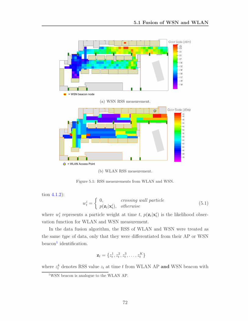
5.1 Fusion of WSN and WLAN
(a) WSN RSS measurement.
(b) WLAN RSS measurement.
Figure 5.1: RSS measurements from WLAN and WSN.
tion 4.1.2):
wit =
{
0, crossing wall particlep(zt|xi
t), otherwise(5.1)
where wit represents a particle weight at time t, p(zt|xi
t) is the likelihood obser-
vation function for WLAN and WSN measurement.
In the data fusion algorithm, the RSS of WLAN and WSN were treated as
the same type of data, only that they were differentiated from their AP or WSN
beacon1 identification.
zt = {z1t , z
2t , z
3t , . . . , z
Kt }
where zkt denotes RSS value zt at time t from WLAN AP and WSN beacon with
1WSN beacon is analogue to the WLAN AP.
72
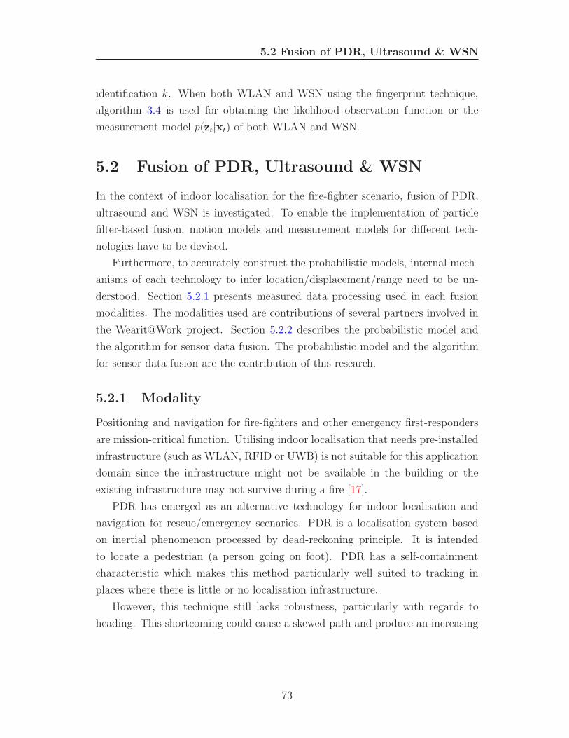
5.2 Fusion of PDR, Ultrasound & WSN
identification k. When both WLAN and WSN using the fingerprint technique,
algorithm 3.4 is used for obtaining the likelihood observation function or the
measurement model p(zt|xt) of both WLAN and WSN.
5.2 Fusion of PDR, Ultrasound & WSN
In the context of indoor localisation for the fire-fighter scenario, fusion of PDR,
ultrasound and WSN is investigated. To enable the implementation of particle
filter-based fusion, motion models and measurement models for different tech-
nologies have to be devised.
Furthermore, to accurately construct the probabilistic models, internal mech-
anisms of each technology to infer location/displacement/range need to be un-
derstood. Section 5.2.1 presents measured data processing used in each fusion
modalities. The modalities used are contributions of several partners involved in
the Wearit@Work project. Section 5.2.2 describes the probabilistic model and
the algorithm for sensor data fusion. The probabilistic model and the algorithm
for sensor data fusion are the contribution of this research.
5.2.1 Modality
Positioning and navigation for fire-fighters and other emergency first-responders
are mission-critical function. Utilising indoor localisation that needs pre-installed
infrastructure (such as WLAN, RFID or UWB) is not suitable for this application
domain since the infrastructure might not be available in the building or the
existing infrastructure may not survive during a fire [17].
PDR has emerged as an alternative technology for indoor localisation and
navigation for rescue/emergency scenarios. PDR is a localisation system based
on inertial phenomenon processed by dead-reckoning principle. It is intended
to locate a pedestrian (a person going on foot). PDR has a self-containment
characteristic which makes this method particularly well suited to tracking in
places where there is little or no localisation infrastructure.
However, this technique still lacks robustness, particularly with regards to
heading. This shortcoming could cause a skewed path and produce an increasing
73
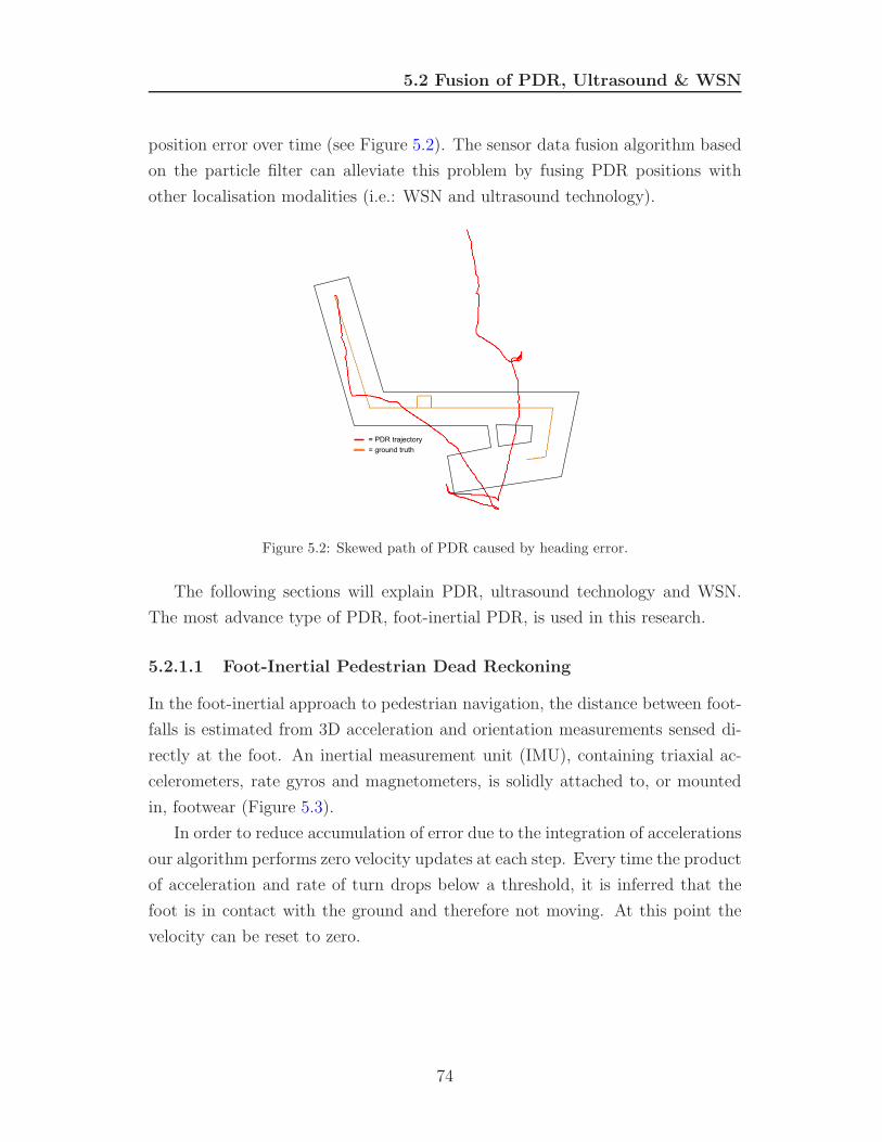
5.2 Fusion of PDR, Ultrasound & WSN
position error over time (see Figure 5.2). The sensor data fusion algorithm based
on the particle filter can alleviate this problem by fusing PDR positions with
other localisation modalities (i.e.: WSN and ultrasound technology).
Figure 5.2: Skewed path of PDR caused by heading error.
The following sections will explain PDR, ultrasound technology and WSN.
The most advance type of PDR, foot-inertial PDR, is used in this research.
5.2.1.1 Foot-Inertial Pedestrian Dead Reckoning
In the foot-inertial approach to pedestrian navigation, the distance between foot-
falls is estimated from 3D acceleration and orientation measurements sensed di-
rectly at the foot. An inertial measurement unit (IMU), containing triaxial ac-
celerometers, rate gyros and magnetometers, is solidly attached to, or mounted
in, footwear (Figure 5.3).
In order to reduce accumulation of error due to the integration of accelerations
our algorithm performs zero velocity updates at each step. Every time the product
of acceleration and rate of turn drops below a threshold, it is inferred that the
foot is in contact with the ground and therefore not moving. At this point the
velocity can be reset to zero.
74
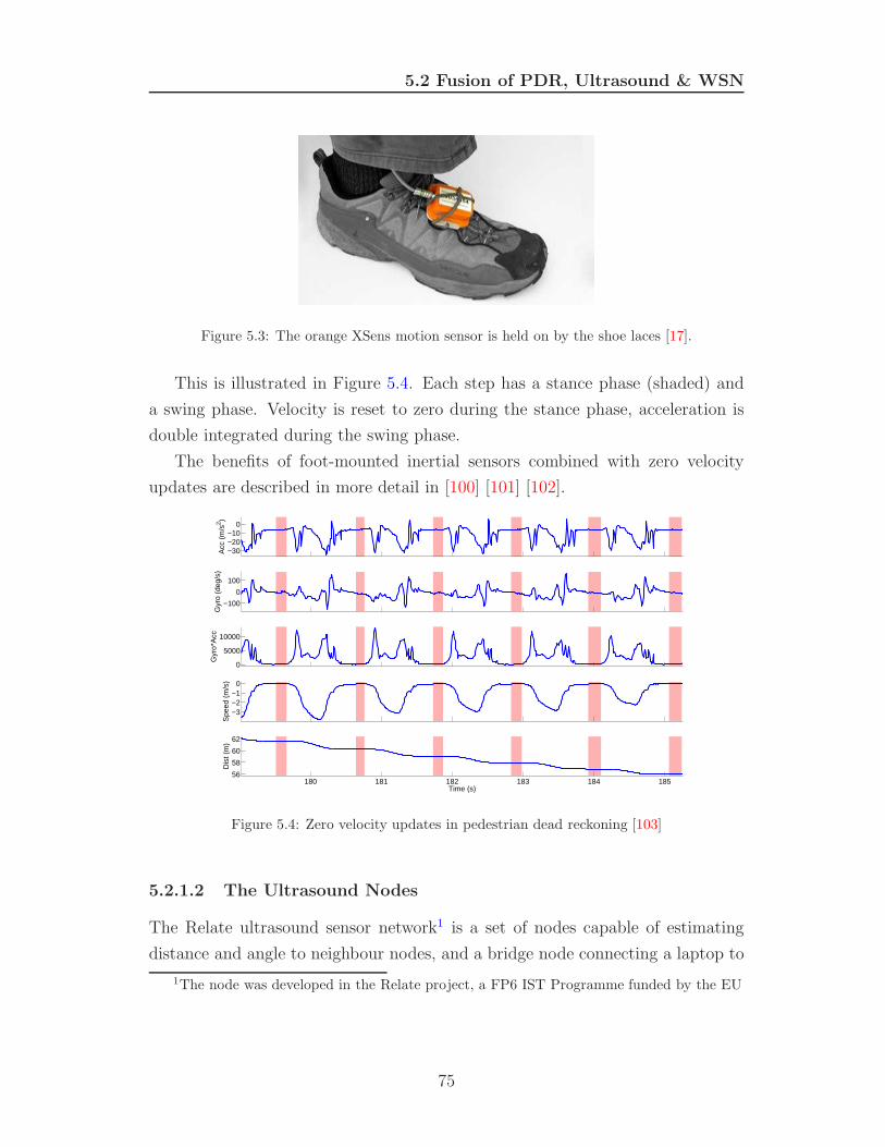
5.2 Fusion of PDR, Ultrasound & WSN
Figure 5.3: The orange XSens motion sensor is held on by the shoe laces [17].
This is illustrated in Figure 5.4. Each step has a stance phase (shaded) and
a swing phase. Velocity is reset to zero during the stance phase, acceleration is
double integrated during the swing phase.
The benefits of foot-mounted inertial sensors combined with zero velocity
updates are described in more detail in [100] [101] [102].
Acc
(m
/s2 )
−30−20−10
0
Gyr
o (d
eg/s
)
−100
0
100
Gyr
o*A
cc
0
5000
10000
Spe
ed (
m/s
)
−3−2−1
0
Dis
t (m
)
Time (s)180 181 182 183 184 185
56
58
60
62
Figure 5.4: Zero velocity updates in pedestrian dead reckoning [103]
5.2.1.2 The Ultrasound Nodes
The Relate ultrasound sensor network1 is a set of nodes capable of estimating
distance and angle to neighbour nodes, and a bridge node connecting a laptop to
1The node was developed in the Relate project, a FP6 IST Programme funded by the EU
75
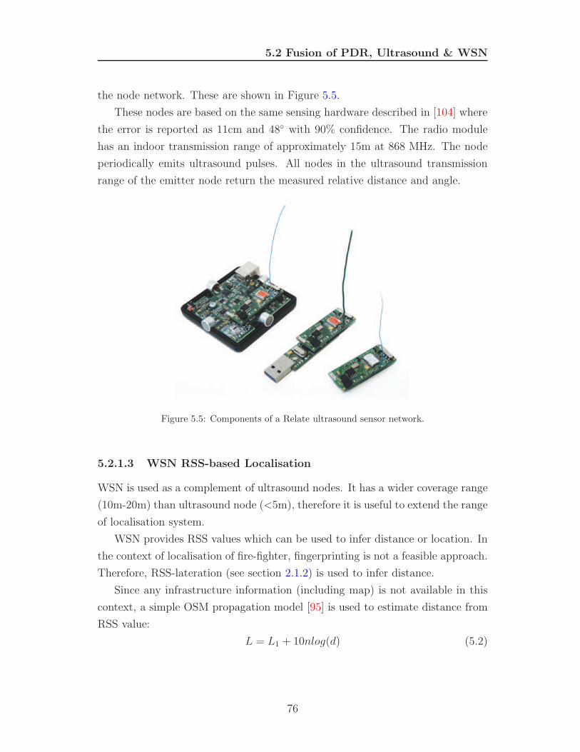
5.2 Fusion of PDR, Ultrasound & WSN
the node network. These are shown in Figure 5.5.
These nodes are based on the same sensing hardware described in [104] where
the error is reported as 11cm and 48◦ with 90% confidence. The radio module
has an indoor transmission range of approximately 15m at 868 MHz. The node
periodically emits ultrasound pulses. All nodes in the ultrasound transmission
range of the emitter node return the measured relative distance and angle.
Figure 5.5: Components of a Relate ultrasound sensor network.
5.2.1.3 WSN RSS-based Localisation
WSN is used as a complement of ultrasound nodes. It has a wider coverage range
(10m-20m) than ultrasound node (<5m), therefore it is useful to extend the range
of localisation system.
WSN provides RSS values which can be used to infer distance or location. In
the context of localisation of fire-fighter, fingerprinting is not a feasible approach.
Therefore, RSS-lateration (see section 2.1.2) is used to infer distance.
Since any infrastructure information (including map) is not available in this
context, a simple OSM propagation model [95] is used to estimate distance from
RSS value:
L = L1 + 10nlog(d) (5.2)
76
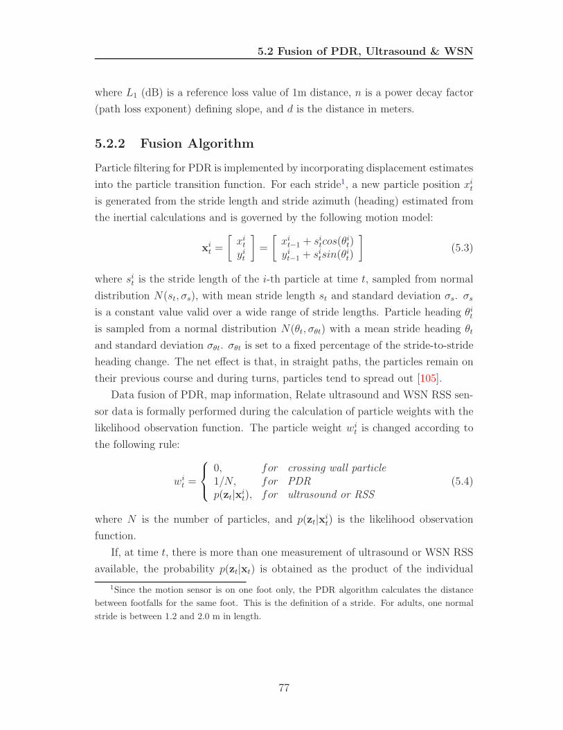
5.2 Fusion of PDR, Ultrasound & WSN
where L1 (dB) is a reference loss value of 1m distance, n is a power decay factor
(path loss exponent) defining slope, and d is the distance in meters.
5.2.2 Fusion Algorithm
Particle filtering for PDR is implemented by incorporating displacement estimates
into the particle transition function. For each stride1, a new particle position xit
is generated from the stride length and stride azimuth (heading) estimated from
the inertial calculations and is governed by the following motion model:
xit =
[
xit
yit
]
=
[
xit−1 + si
tcos(θit)
yit−1 + si
tsin(θit)
]
(5.3)
where sit is the stride length of the i-th particle at time t, sampled from normal
distribution N(st, σs), with mean stride length st and standard deviation σs. σs
is a constant value valid over a wide range of stride lengths. Particle heading θit
is sampled from a normal distribution N(θt, σθt) with a mean stride heading θt
and standard deviation σθt. σθt is set to a fixed percentage of the stride-to-stride
heading change. The net effect is that, in straight paths, the particles remain on
their previous course and during turns, particles tend to spread out [105].
Data fusion of PDR, map information, Relate ultrasound and WSN RSS sen-
sor data is formally performed during the calculation of particle weights with the
likelihood observation function. The particle weight wit is changed according to
the following rule:
wit =
0, for crossing wall particle1/N, for PDRp(zt|xi
t), for ultrasound or RSS(5.4)
where N is the number of particles, and p(zt|xit) is the likelihood observation
function.
If, at time t, there is more than one measurement of ultrasound or WSN RSS
available, the probability p(zt|xt) is obtained as the product of the individual
1Since the motion sensor is on one foot only, the PDR algorithm calculates the distance
between footfalls for the same foot. This is the definition of a stride. For adults, one normal
stride is between 1.2 and 2.0 m in length.
77
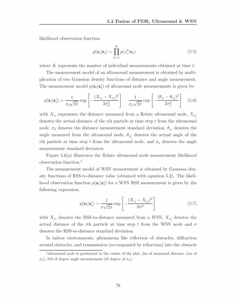
5.2 Fusion of PDR, Ultrasound & WSN
likelihood observation function.
p(zt|xt) =
K∏
k=1
p(zkt |xt) (5.5)
where K represents the number of individual measurements obtained at time t.
The measurement model of an ultrasound measurement is obtained by multi-
plication of two Gaussian density functions of distance and angle measurement.
The measurement model p(zt|xit) of ultrasound node measurements is given by:
p(zt|xit) =
1
σd
√2π
exp
[
−(Xzt
− Xxit)2
2σ2d
]
.1
σa
√2π
exp
[
−(θzt
− θxit)2
2σ2a
]
(5.6)
with Xztrepresents the distance measured from a Relate ultrasound node, Xxi
t
denotes the actual distance of the ith particle at time step t from the ultrasound
node, σd denotes the distance measurement standard deviation, θztdenotes the
angle measured from the ultrasound node, θxit
denotes the actual angle of the
ith particle at time step t from the ultrasound node, and σa denotes the angle
measurement standard deviation.
Figure 5.6(a) illustrates the Relate ultrasound node measurement likelihood
observation function.1
The measurement model of WSN measurement is obtained by Gaussian den-
sity functions of RSS-to-distance value (obtained with equation 5.2). The likeli-
hood observation function p(zt|xit) for a WSN RSS measurement is given by the
following expression:
p(zt|xit) =
1
σ√
2πexp
[
−(Xzt
− Xxit)2
2σ2
]
(5.7)
with Xztdenotes the RSS-to-distance measured from a WSN, Xxi
tdenotes the
actual distance of the ith particle at time step t from the WSN node and σ
denotes the RSS-to-distance standard deviation.
In indoor environments, phenomena like reflection of obstacles, diffraction
around obstacles, and transmission (accompanied by refraction) into the obstacle
1ultrasound node is positioned in the centre of the plot, 2m of measured distance (1m of
σd), 210 of degree angle measurement (45 degree of σa).
78
5.2 Fusion of PDR, Ultrasound & WSN
0
2
4
6
8
100 1 2 3 4 5 6 7 8 9 10
0
2
4x 10
−3
X−Axis
Pro
babi
lity
Y−Axis
(a) Likelihood observation function of ultrasound measurement
0
2
4
6
8
100 1 2 3 4 5 6 7 8 9 10
0
0.5
1x 10
−3
X−axis
Pro
babi
lity
Y−axis
(b) Likelihood observation function of WSN RSS measurement
Figure 5.6: Likelihood observation functions of the ultrasound and WSN measurement
or medium, considerably reduce the reliability of distances computed from RSS
values.
To cope with this, a relatively high value for the standard deviation σ of the
RSS-to-distance measurement (0.5 of d) is used. Figure 5.6(b) illustrates the
WSN node likelihood observation function.1
1WSN node is positioned in the centre, 2m of RSS-to-distance measurement (1m of σ).
79
5.3 Conclusion
5.3 Conclusion
In this chapter, the usage of particle filter-based algorithm for sensor data fusion
of multi-modal localisation technology was described. The sensor data fusion was
investigated to achieve more fine-grained of an opportunistic indoor localisation.
In the context of localisation in car industry, fusion of WSN and WLAN was
investigated. It was found that RSS values of WSN gives distinctive measurement
probability between fingerprinting grids. Eventually, it leads to better localisation
accuracy when WLAN and WSN are fused. In the data fusion algorithm, the RSS
of WLAN and WSN use the same measurement model explained in algorithm 3.4.
Fusion of PDR, ultrasound and WSN was investigated to increase the accuracy
of indoor localisation for the fire-fighters. Motion and measurement models of
PDR, ultrasound and WSN were devised to enable the fusion. Fusion for PDR was
implemented by incorporating displacement estimates into the particle motion
model. Novel motion models based on Gaussian density function were devised
for ultrasound and WSN to enable the fusion.
The fusion of opportunistic systems with different technologies through the
development of sensor-specific probabilistic models is one of the contributions of
this research.
The next chapter will present the evaluation of the developed algorithms in
the opportunistic indoor localisation system.
80
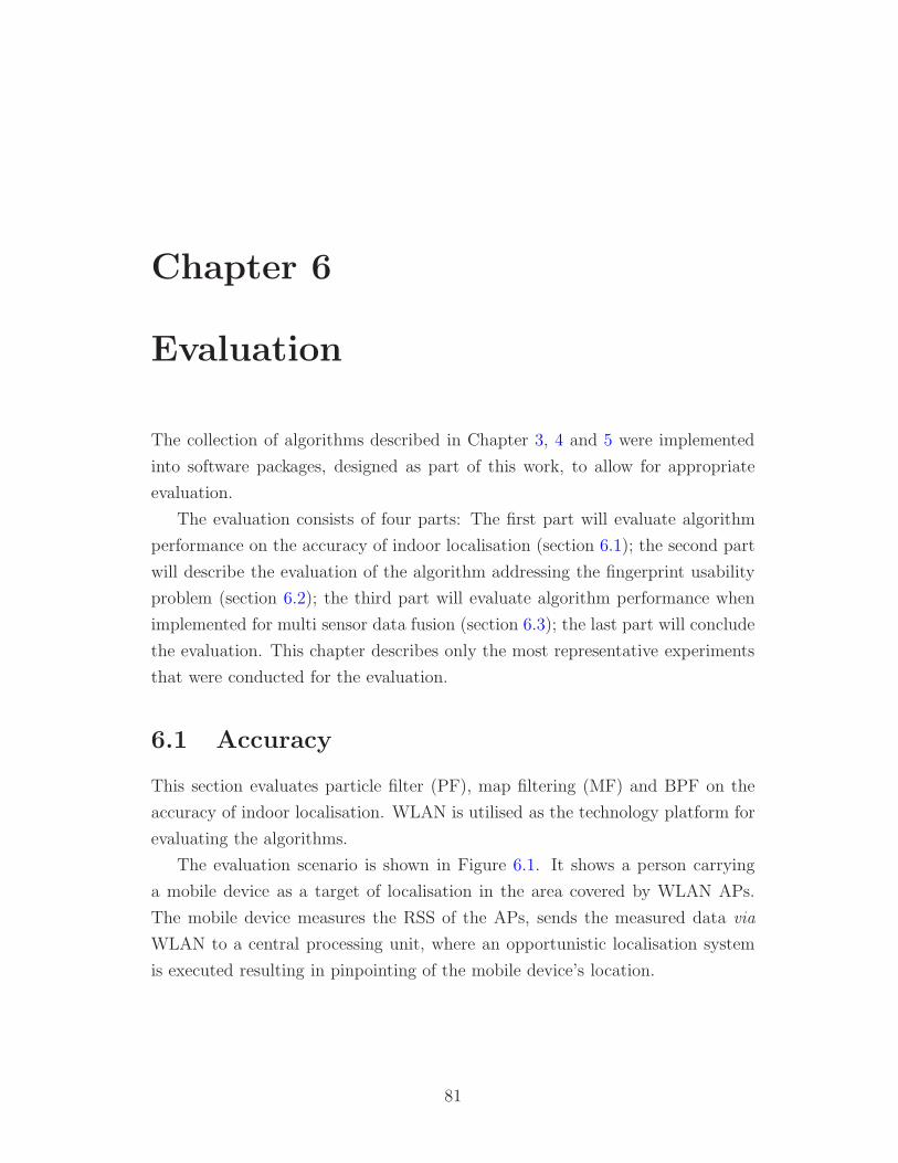
Chapter 6
Evaluation
The collection of algorithms described in Chapter 3, 4 and 5 were implemented
into software packages, designed as part of this work, to allow for appropriate
evaluation.
The evaluation consists of four parts: The first part will evaluate algorithm
performance on the accuracy of indoor localisation (section 6.1); the second part
will describe the evaluation of the algorithm addressing the fingerprint usability
problem (section 6.2); the third part will evaluate algorithm performance when
implemented for multi sensor data fusion (section 6.3); the last part will conclude
the evaluation. This chapter describes only the most representative experiments
that were conducted for the evaluation.
6.1 Accuracy
This section evaluates particle filter (PF), map filtering (MF) and BPF on the
accuracy of indoor localisation. WLAN is utilised as the technology platform for
evaluating the algorithms.
The evaluation scenario is shown in Figure 6.1. It shows a person carrying
a mobile device as a target of localisation in the area covered by WLAN APs.
The mobile device measures the RSS of the APs, sends the measured data via
WLAN to a central processing unit, where an opportunistic localisation system
is executed resulting in pinpointing of the mobile device’s location.
81
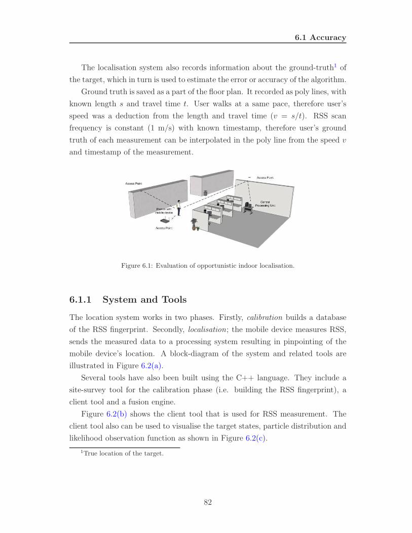
6.1 Accuracy
The localisation system also records information about the ground-truth1 of
the target, which in turn is used to estimate the error or accuracy of the algorithm.
Ground truth is saved as a part of the floor plan. It recorded as poly lines, with
known length s and travel time t. User walks at a same pace, therefore user’s
speed was a deduction from the length and travel time (v = s/t). RSS scan
frequency is constant (1 m/s) with known timestamp, therefore user’s ground
truth of each measurement can be interpolated in the poly line from the speed v
and timestamp of the measurement.
Figure 6.1: Evaluation of opportunistic indoor localisation.
6.1.1 System and Tools
The location system works in two phases. Firstly, calibration builds a database
of the RSS fingerprint. Secondly, localisation; the mobile device measures RSS,
sends the measured data to a processing system resulting in pinpointing of the
mobile device’s location. A block-diagram of the system and related tools are
illustrated in Figure 6.2(a).
Several tools have also been built using the C++ language. They include a
site-survey tool for the calibration phase (i.e. building the RSS fingerprint), a
client tool and a fusion engine.
Figure 6.2(b) shows the client tool that is used for RSS measurement. The
client tool also can be used to visualise the target states, particle distribution and
likelihood observation function as shown in Figure 6.2(c).
1True location of the target.
82
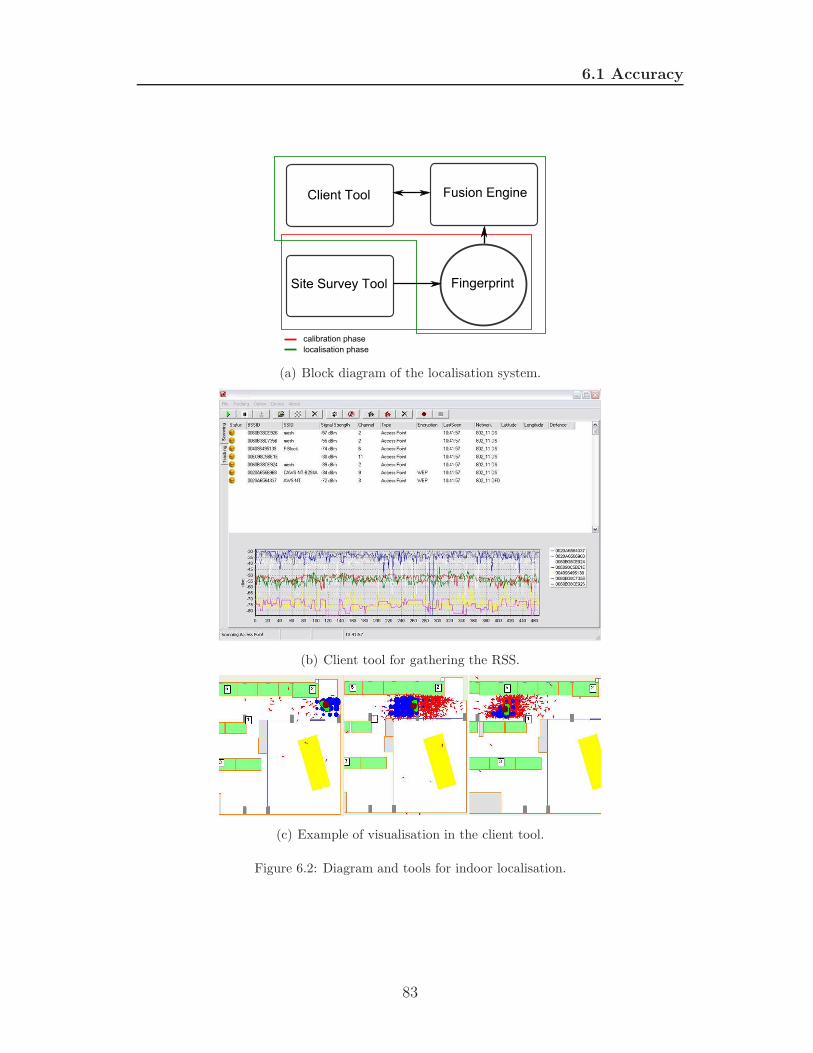
6.1 Accuracy
(a) Block diagram of the localisation system.
(b) Client tool for gathering the RSS.
(c) Example of visualisation in the client tool.
Figure 6.2: Diagram and tools for indoor localisation.
83
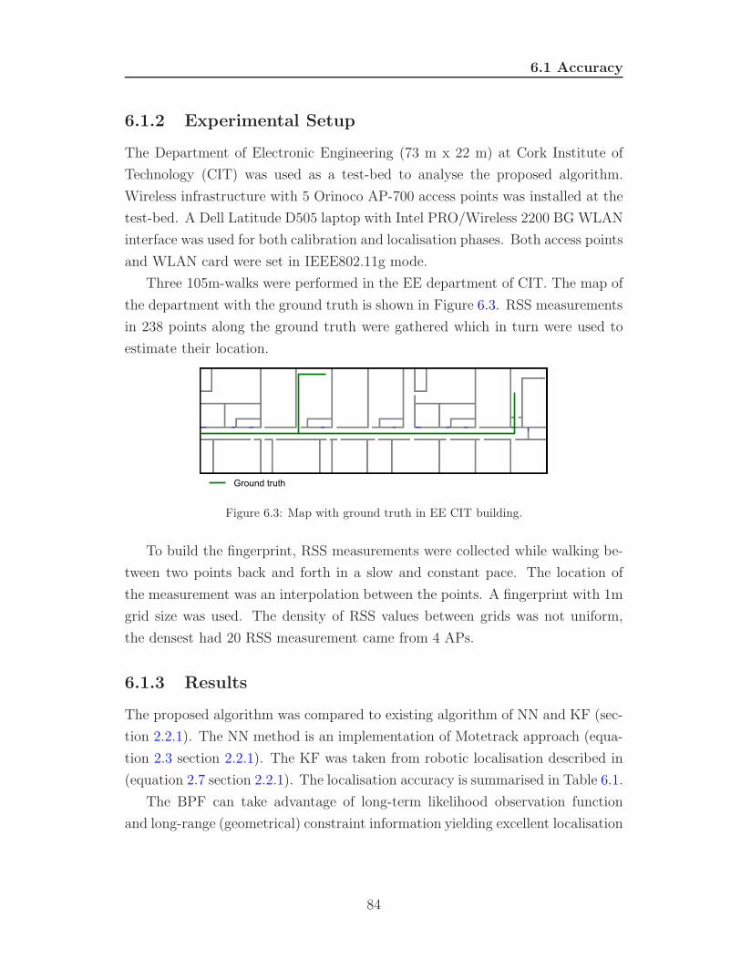
6.1 Accuracy
6.1.2 Experimental Setup
The Department of Electronic Engineering (73 m x 22 m) at Cork Institute of
Technology (CIT) was used as a test-bed to analyse the proposed algorithm.
Wireless infrastructure with 5 Orinoco AP-700 access points was installed at the
test-bed. A Dell Latitude D505 laptop with Intel PRO/Wireless 2200 BG WLAN
interface was used for both calibration and localisation phases. Both access points
and WLAN card were set in IEEE802.11g mode.
Three 105m-walks were performed in the EE department of CIT. The map of
the department with the ground truth is shown in Figure 6.3. RSS measurements
in 238 points along the ground truth were gathered which in turn were used to
estimate their location.
Figure 6.3: Map with ground truth in EE CIT building.
To build the fingerprint, RSS measurements were collected while walking be-
tween two points back and forth in a slow and constant pace. The location of
the measurement was an interpolation between the points. A fingerprint with 1m
grid size was used. The density of RSS values between grids was not uniform,
the densest had 20 RSS measurement came from 4 APs.
6.1.3 Results
The proposed algorithm was compared to existing algorithm of NN and KF (sec-
tion 2.2.1). The NN method is an implementation of Motetrack approach (equa-
tion 2.3 section 2.2.1). The KF was taken from robotic localisation described in
(equation 2.7 section 2.2.1). The localisation accuracy is summarised in Table 6.1.
The BPF can take advantage of long-term likelihood observation function
and long-range (geometrical) constraint information yielding excellent localisation
84
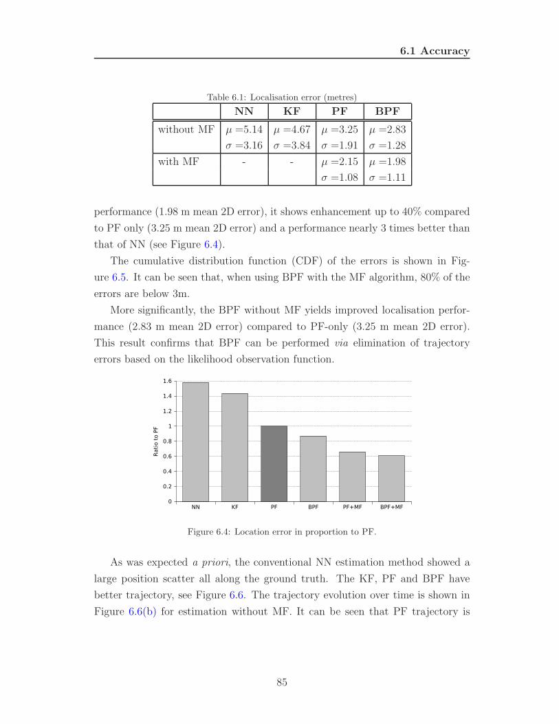
6.1 Accuracy
Table 6.1: Localisation error (metres)
NN KF PF BPF
without MF µ =5.14 µ =4.67 µ =3.25 µ =2.83
σ =3.16 σ =3.84 σ =1.91 σ =1.28
with MF - - µ =2.15 µ =1.98
σ =1.08 σ =1.11
performance (1.98 m mean 2D error), it shows enhancement up to 40% compared
to PF only (3.25 m mean 2D error) and a performance nearly 3 times better than
that of NN (see Figure 6.4).
The cumulative distribution function (CDF) of the errors is shown in Fig-
ure 6.5. It can be seen that, when using BPF with the MF algorithm, 80% of the
errors are below 3m.
More significantly, the BPF without MF yields improved localisation perfor-
mance (2.83 m mean 2D error) compared to PF-only (3.25 m mean 2D error).
This result confirms that BPF can be performed via elimination of trajectory
errors based on the likelihood observation function.
NN KF PF BPF PF+MF BPF+MF0
0.2
0.4
0.6
0.8
1
1.2
1.4
1.6
Rati
o t
o P
F
Figure 6.4: Location error in proportion to PF.
As was expected a priori, the conventional NN estimation method showed a
large position scatter all along the ground truth. The KF, PF and BPF have
better trajectory, see Figure 6.6. The trajectory evolution over time is shown in
Figure 6.6(b) for estimation without MF. It can be seen that PF trajectory is
85
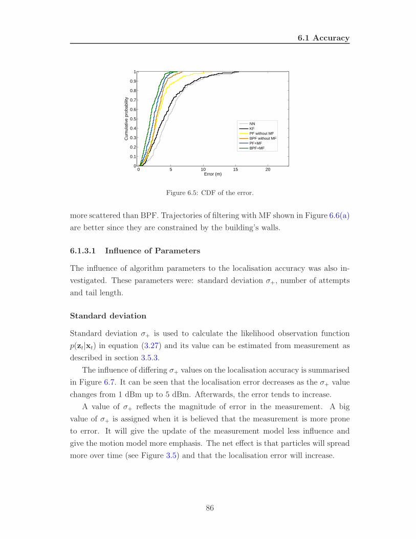
6.1 Accuracy
0 5 10 15 200
0.1
0.2
0.3
0.4
0.5
0.6
0.7
0.8
0.9
1
Error (m)
Cum
ulat
ive
prob
abili
ty
NNKFPF without MFBPF without MFPF+MFBPF+MF
Figure 6.5: CDF of the error.
more scattered than BPF. Trajectories of filtering with MF shown in Figure 6.6(a)
are better since they are constrained by the building’s walls.
6.1.3.1 Influence of Parameters
The influence of algorithm parameters to the localisation accuracy was also in-
vestigated. These parameters were: standard deviation σ+, number of attempts
and tail length.
Standard deviation
Standard deviation σ+ is used to calculate the likelihood observation function
p(zt|xt) in equation (3.27) and its value can be estimated from measurement as
described in section 3.5.3.
The influence of differing σ+ values on the localisation accuracy is summarised
in Figure 6.7. It can be seen that the localisation error decreases as the σ+ value
changes from 1 dBm up to 5 dBm. Afterwards, the error tends to increase.
A value of σ+ reflects the magnitude of error in the measurement. A big
value of σ+ is assigned when it is believed that the measurement is more prone
to error. It will give the update of the measurement model less influence and
give the motion model more emphasis. The net effect is that particles will spread
more over time (see Figure 3.5) and that the localisation error will increase.
86
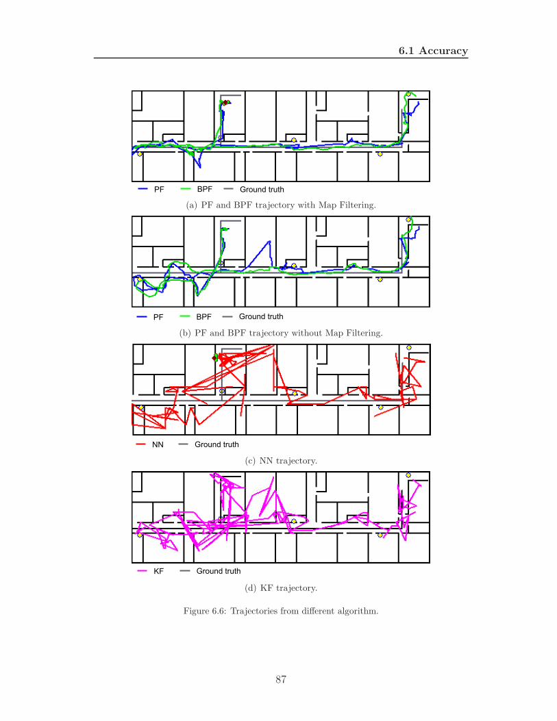
6.1 Accuracy
(a) PF and BPF trajectory with Map Filtering.
(b) PF and BPF trajectory without Map Filtering.
(c) NN trajectory.
(d) KF trajectory.
Figure 6.6: Trajectories from different algorithm.
87
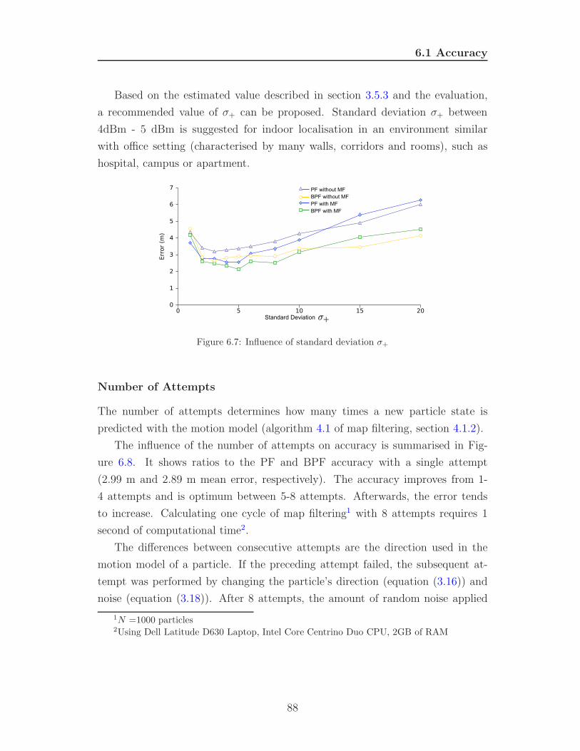
6.1 Accuracy
Based on the estimated value described in section 3.5.3 and the evaluation,
a recommended value of σ+ can be proposed. Standard deviation σ+ between
4dBm - 5 dBm is suggested for indoor localisation in an environment similar
with office setting (characterised by many walls, corridors and rooms), such as
hospital, campus or apartment.
Figure 6.7: Influence of standard deviation σ+
Number of Attempts
The number of attempts determines how many times a new particle state is
predicted with the motion model (algorithm 4.1 of map filtering, section 4.1.2).
The influence of the number of attempts on accuracy is summarised in Fig-
ure 6.8. It shows ratios to the PF and BPF accuracy with a single attempt
(2.99 m and 2.89 m mean error, respectively). The accuracy improves from 1-
4 attempts and is optimum between 5-8 attempts. Afterwards, the error tends
to increase. Calculating one cycle of map filtering1 with 8 attempts requires 1
second of computational time2.
The differences between consecutive attempts are the direction used in the
motion model of a particle. If the preceding attempt failed, the subsequent at-
tempt was performed by changing the particle’s direction (equation (3.16)) and
noise (equation (3.18)). After 8 attempts, the amount of random noise applied
1N =1000 particles2Using Dell Latitude D630 Laptop, Intel Core Centrino Duo CPU, 2GB of RAM
88
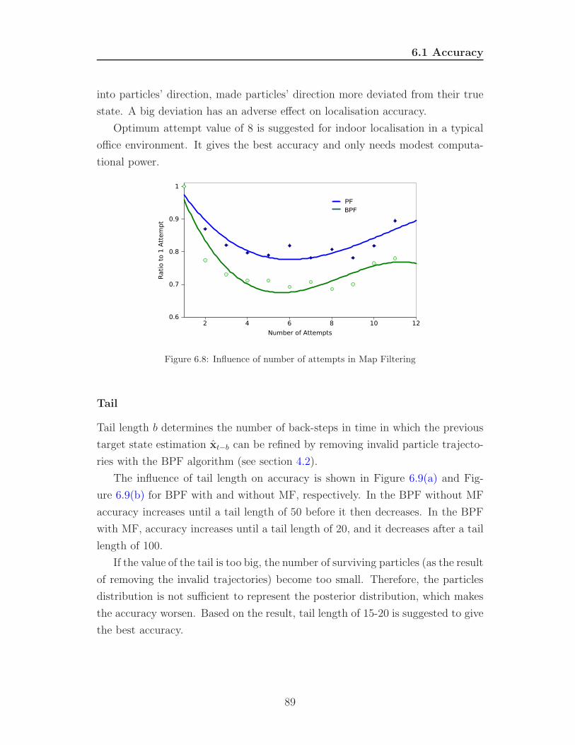
6.1 Accuracy
into particles’ direction, made particles’ direction more deviated from their true
state. A big deviation has an adverse effect on localisation accuracy.
Optimum attempt value of 8 is suggested for indoor localisation in a typical
office environment. It gives the best accuracy and only needs modest computa-
tional power.
Figure 6.8: Influence of number of attempts in Map Filtering
Tail
Tail length b determines the number of back-steps in time in which the previous
target state estimation xt−b can be refined by removing invalid particle trajecto-
ries with the BPF algorithm (see section 4.2).
The influence of tail length on accuracy is shown in Figure 6.9(a) and Fig-
ure 6.9(b) for BPF with and without MF, respectively. In the BPF without MF
accuracy increases until a tail length of 50 before it then decreases. In the BPF
with MF, accuracy increases until a tail length of 20, and it decreases after a tail
length of 100.
If the value of the tail is too big, the number of surviving particles (as the result
of removing the invalid trajectories) become too small. Therefore, the particles
distribution is not sufficient to represent the posterior distribution, which makes
the accuracy worsen. Based on the result, tail length of 15-20 is suggested to give
the best accuracy.
89
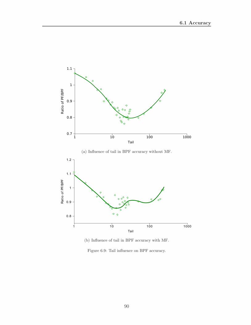
6.1 Accuracy
(a) Influence of tail in BPF accuracy without MF.
(b) Influence of tail in BPF accuracy with MF.
Figure 6.9: Tail influence on BPF accuracy.
90
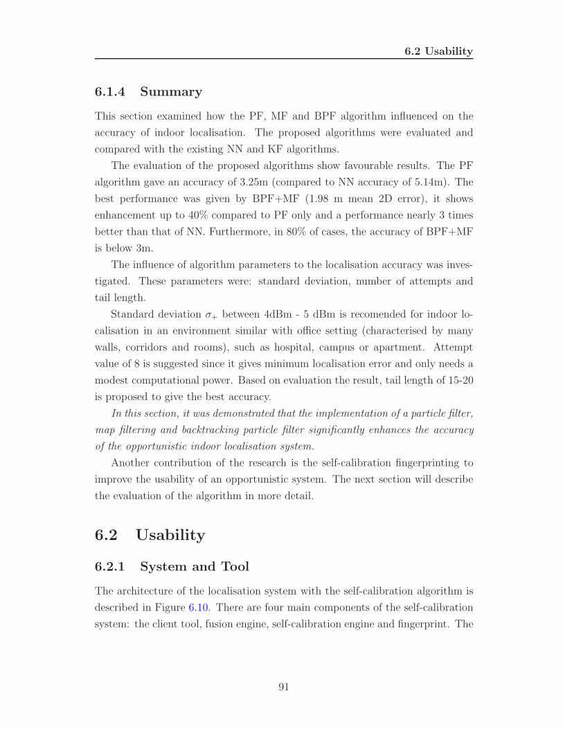
6.2 Usability
6.1.4 Summary
This section examined how the PF, MF and BPF algorithm influenced on the
accuracy of indoor localisation. The proposed algorithms were evaluated and
compared with the existing NN and KF algorithms.
The evaluation of the proposed algorithms show favourable results. The PF
algorithm gave an accuracy of 3.25m (compared to NN accuracy of 5.14m). The
best performance was given by BPF+MF (1.98 m mean 2D error), it shows
enhancement up to 40% compared to PF only and a performance nearly 3 times
better than that of NN. Furthermore, in 80% of cases, the accuracy of BPF+MF
is below 3m.
The influence of algorithm parameters to the localisation accuracy was inves-
tigated. These parameters were: standard deviation, number of attempts and
tail length.
Standard deviation σ+ between 4dBm - 5 dBm is recomended for indoor lo-
calisation in an environment similar with office setting (characterised by many
walls, corridors and rooms), such as hospital, campus or apartment. Attempt
value of 8 is suggested since it gives minimum localisation error and only needs a
modest computational power. Based on evaluation the result, tail length of 15-20
is proposed to give the best accuracy.
In this section, it was demonstrated that the implementation of a particle filter,
map filtering and backtracking particle filter significantly enhances the accuracy
of the opportunistic indoor localisation system.
Another contribution of the research is the self-calibration fingerprinting to
improve the usability of an opportunistic system. The next section will describe
the evaluation of the algorithm in more detail.
6.2 Usability
6.2.1 System and Tool
The architecture of the localisation system with the self-calibration algorithm is
described in Figure 6.10. There are four main components of the self-calibration
system: the client tool, fusion engine, self-calibration engine and fingerprint. The
91
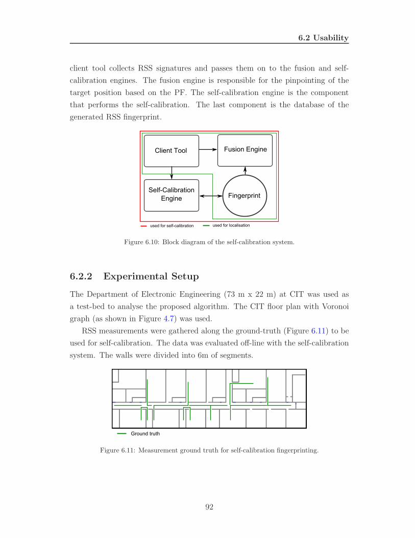
6.2 Usability
client tool collects RSS signatures and passes them on to the fusion and self-
calibration engines. The fusion engine is responsible for the pinpointing of the
target position based on the PF. The self-calibration engine is the component
that performs the self-calibration. The last component is the database of the
generated RSS fingerprint.
Figure 6.10: Block diagram of the self-calibration system.
6.2.2 Experimental Setup
The Department of Electronic Engineering (73 m x 22 m) at CIT was used as
a test-bed to analyse the proposed algorithm. The CIT floor plan with Voronoi
graph (as shown in Figure 4.7) was used.
RSS measurements were gathered along the ground-truth (Figure 6.11) to be
used for self-calibration. The data was evaluated off-line with the self-calibration
system. The walls were divided into 6m of segments.
Figure 6.11: Measurement ground truth for self-calibration fingerprinting.
92
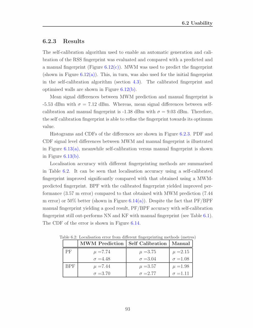
6.2 Usability
6.2.3 Results
The self-calibration algorithm used to enable an automatic generation and cali-
bration of the RSS fingerprint was evaluated and compared with a predicted and
a manual fingerprint (Figure 6.12(c)). MWM was used to predict the fingerprint
(shown in Figure 6.12(a)). This, in turn, was also used for the initial fingerprint
in the self-calibration algorithm (section 4.3). The calibrated fingerprint and
optimised walls are shown in Figure 6.12(b).
Mean signal differences between MWM prediction and manual fingerprint is
-5.53 dBm with σ = 7.12 dBm. Whereas, mean signal differences between self-
calibration and manual fingerprint is -1.38 dBm with σ = 9.03 dBm. Therefore,
the self calibration fingerprint is able to refine the fingerprint towards its optimum
value.
Histograms and CDFs of the differences are shown in Figure 6.2.3. PDF and
CDF signal level differences between MWM and manual fingerprint is illustrated
in Figure 6.13(a), meanwhile self-calibration versus manual fingerprint is shown
in Figure 6.13(b).
Localisation accuracy with different fingerprinting methods are summarised
in Table 6.2. It can be seen that localisation accuracy using a self-calibrated
fingerprint improved significantly compared with that obtained using a MWM-
predicted fingerprint. BPF with the calibrated fingerprint yielded improved per-
formance (3.57 m error) compared to that obtained with MWM prediction (7.44
m error) or 50% better (shown in Figure 6.14(a)). Despite the fact that PF/BPF
manual fingerprint yielding a good result, PF/BPF accuracy with self-calibration
fingerprint still out-performs NN and KF with manual fingerprint (see Table 6.1).
The CDF of the error is shown in Figure 6.14.
Table 6.2: Localisation error from different fingerprinting methods (metres)
MWM Prediction Self Calibration Manual
PF µ =7.74 µ =3.75 µ =2.15
σ =4.48 σ =3.04 σ =1.08
BPF µ =7.44 µ =3.57 µ =1.98
σ =3.70 σ =2.77 σ =1.11
93
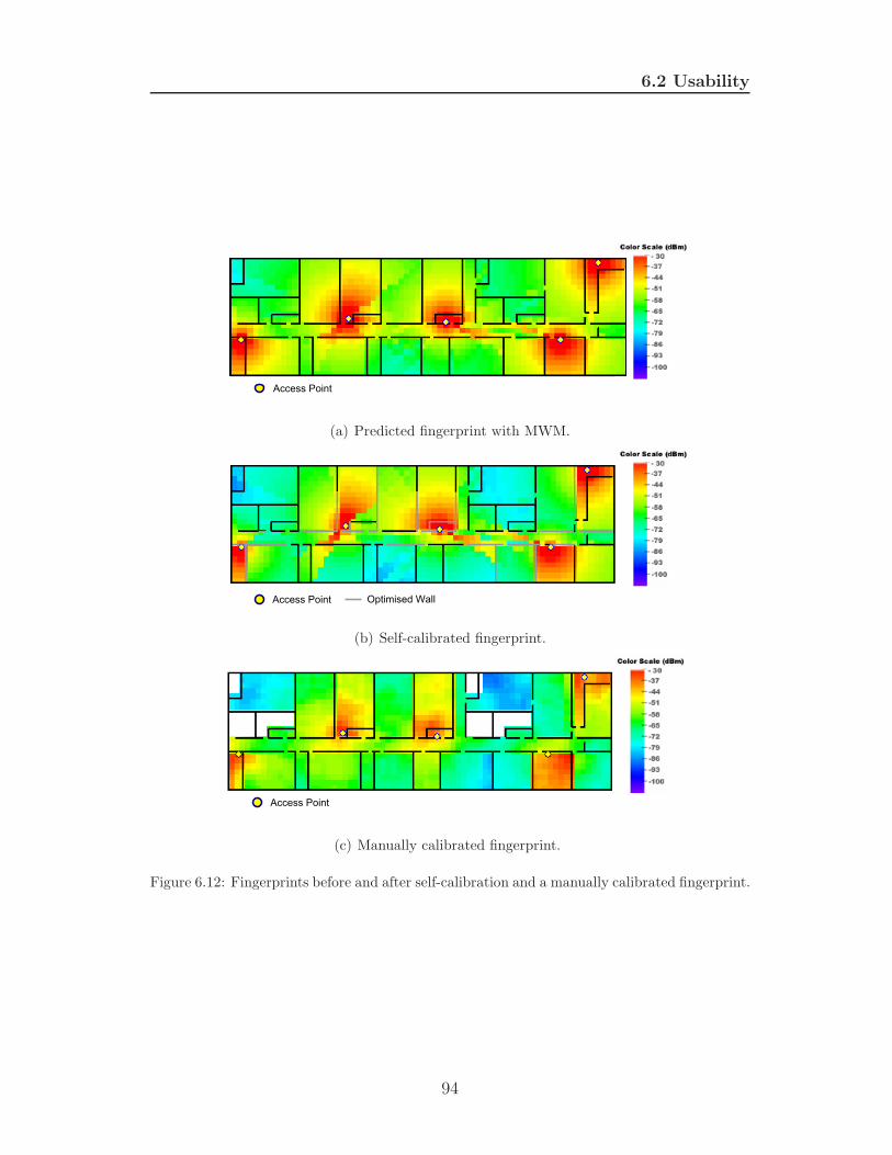
6.2 Usability
(a) Predicted fingerprint with MWM.
(b) Self-calibrated fingerprint.
(c) Manually calibrated fingerprint.
Figure 6.12: Fingerprints before and after self-calibration and a manually calibrated fingerprint.
94
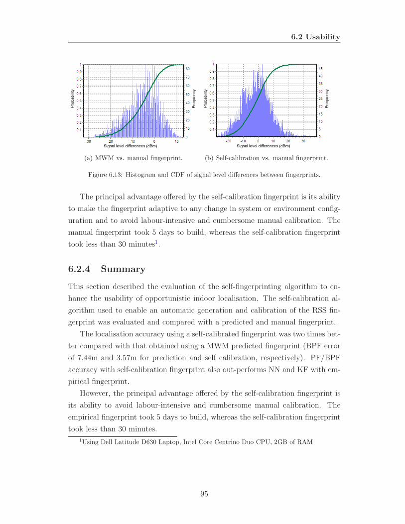
6.2 Usability
(a) MWM vs. manual fingerprint. (b) Self-calibration vs. manual fingerprint.
Figure 6.13: Histogram and CDF of signal level differences between fingerprints.
The principal advantage offered by the self-calibration fingerprint is its ability
to make the fingerprint adaptive to any change in system or environment config-
uration and to avoid labour-intensive and cumbersome manual calibration. The
manual fingerprint took 5 days to build, whereas the self-calibration fingerprint
took less than 30 minutes1.
6.2.4 Summary
This section described the evaluation of the self-fingerprinting algorithm to en-
hance the usability of opportunistic indoor localisation. The self-calibration al-
gorithm used to enable an automatic generation and calibration of the RSS fin-
gerprint was evaluated and compared with a predicted and manual fingerprint.
The localisation accuracy using a self-calibrated fingerprint was two times bet-
ter compared with that obtained using a MWM predicted fingerprint (BPF error
of 7.44m and 3.57m for prediction and self calibration, respectively). PF/BPF
accuracy with self-calibration fingerprint also out-performs NN and KF with em-
pirical fingerprint.
However, the principal advantage offered by the self-calibration fingerprint is
its ability to avoid labour-intensive and cumbersome manual calibration. The
empirical fingerprint took 5 days to build, whereas the self-calibration fingerprint
took less than 30 minutes.
1Using Dell Latitude D630 Laptop, Intel Core Centrino Duo CPU, 2GB of RAM
95
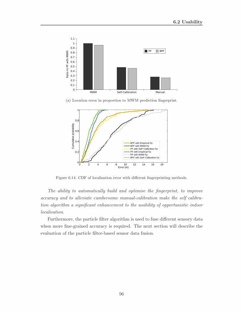
6.2 Usability
(a) Location error in proportion to MWM prediction fingerprint.
0 2 4 6 8 10 12 14 16 180
0.2
0.4
0.6
0.8
1
Error (m)
Cum
ulat
ive
prob
abili
ty
BPF with Empirical FpBPF with MWM FpPF with Self−Calibration FpPF with Empirical FpPF with MWM FpBPF with Self−Calibration Fp
Figure 6.14: CDF of localisation error with different fingerprinting methods.
The ability to automatically build and optimise the fingerprint, to improve
accuracy and to alleviate cumbersome manual-calibration make the self calibra-
tion algorithm a significant enhancement to the usability of opportunistic indoor
localisation.
Furthermore, the particle filter algorithm is used to fuse different sensory data
when more fine-grained accuracy is required. The next section will describe the
evaluation of the particle filter-based sensor data fusion.
96
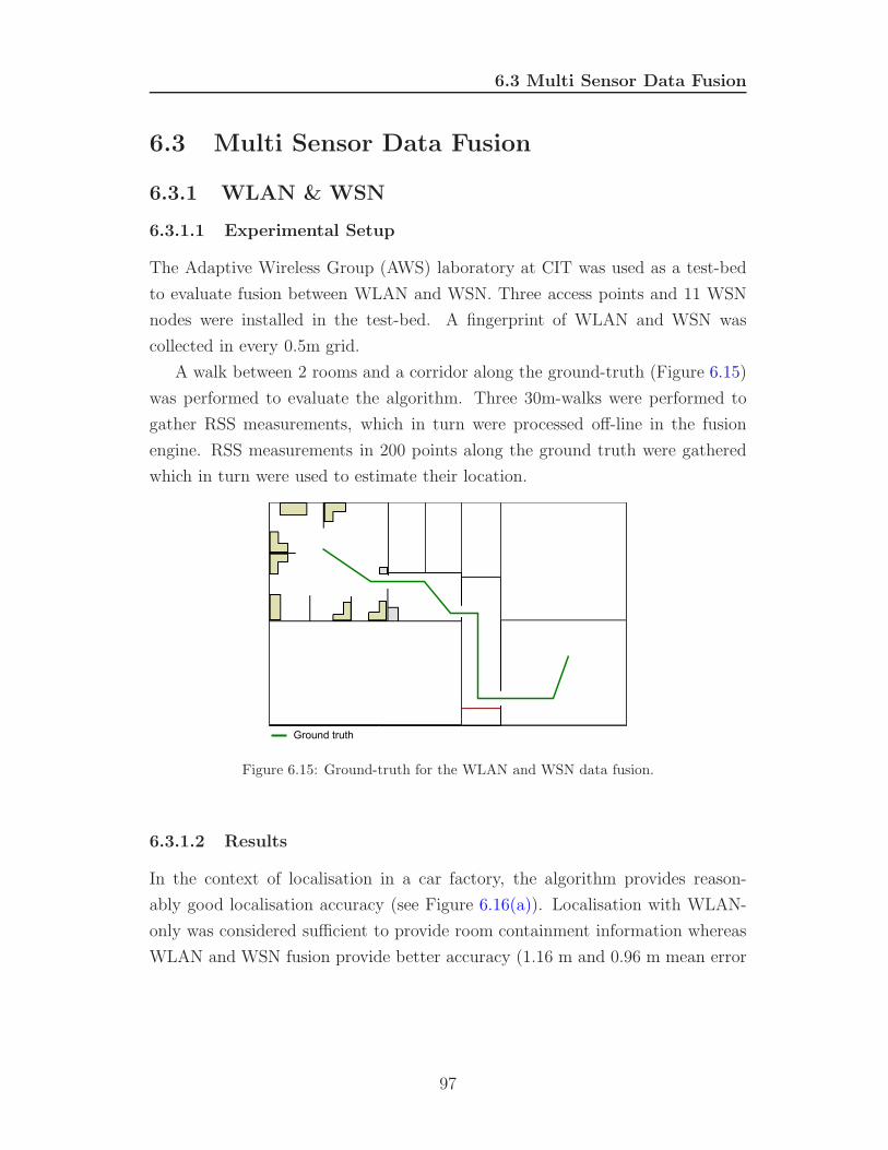
6.3 Multi Sensor Data Fusion
6.3 Multi Sensor Data Fusion
6.3.1 WLAN & WSN
6.3.1.1 Experimental Setup
The Adaptive Wireless Group (AWS) laboratory at CIT was used as a test-bed
to evaluate fusion between WLAN and WSN. Three access points and 11 WSN
nodes were installed in the test-bed. A fingerprint of WLAN and WSN was
collected in every 0.5m grid.
A walk between 2 rooms and a corridor along the ground-truth (Figure 6.15)
was performed to evaluate the algorithm. Three 30m-walks were performed to
gather RSS measurements, which in turn were processed off-line in the fusion
engine. RSS measurements in 200 points along the ground truth were gathered
which in turn were used to estimate their location.
Figure 6.15: Ground-truth for the WLAN and WSN data fusion.
6.3.1.2 Results
In the context of localisation in a car factory, the algorithm provides reason-
ably good localisation accuracy (see Figure 6.16(a)). Localisation with WLAN-
only was considered sufficient to provide room containment information whereas
WLAN and WSN fusion provide better accuracy (1.16 m and 0.96 m mean error
97
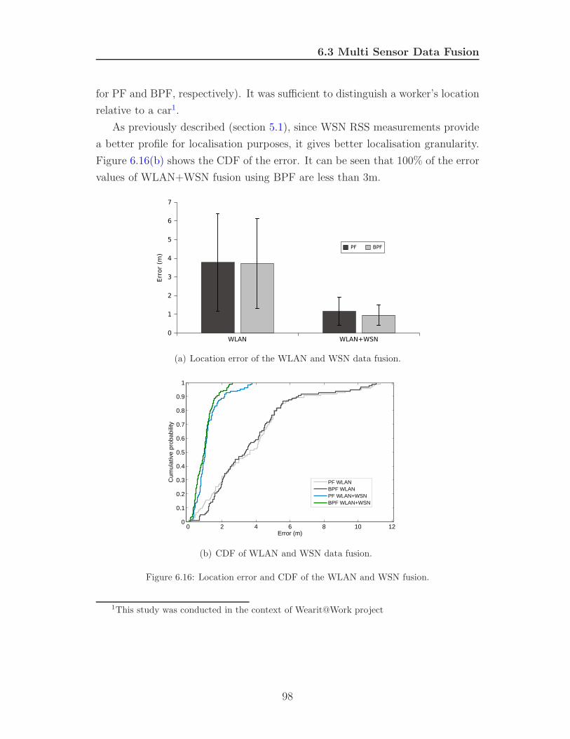
6.3 Multi Sensor Data Fusion
for PF and BPF, respectively). It was sufficient to distinguish a worker’s location
relative to a car1.
As previously described (section 5.1), since WSN RSS measurements provide
a better profile for localisation purposes, it gives better localisation granularity.
Figure 6.16(b) shows the CDF of the error. It can be seen that 100% of the error
values of WLAN+WSN fusion using BPF are less than 3m.
WLAN WLAN+WSN0
1
2
3
4
5
6
7
Err
or
(m)
PF BPF
(a) Location error of the WLAN and WSN data fusion.
0 2 4 6 8 10 120
0.1
0.2
0.3
0.4
0.5
0.6
0.7
0.8
0.9
1
Error (m)
Cum
ulat
ive
prob
abili
ty
PF WLANBPF WLANPF WLAN+WSNBPF WLAN+WSN
(b) CDF of WLAN and WSN data fusion.
Figure 6.16: Location error and CDF of the WLAN and WSN fusion.
1This study was conducted in the context of Wearit@Work project
98
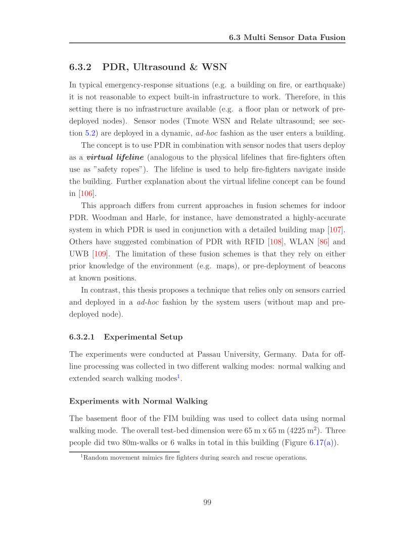
6.3 Multi Sensor Data Fusion
6.3.2 PDR, Ultrasound & WSN
In typical emergency-response situations (e.g. a building on fire, or earthquake)
it is not reasonable to expect built-in infrastructure to work. Therefore, in this
setting there is no infrastructure available (e.g. a floor plan or network of pre-
deployed nodes). Sensor nodes (Tmote WSN and Relate ultrasound; see sec-
tion 5.2) are deployed in a dynamic, ad-hoc fashion as the user enters a building.
The concept is to use PDR in combination with sensor nodes that users deploy
as a virtual lifeline (analogous to the physical lifelines that fire-fighters often
use as ”safety ropes”). The lifeline is used to help fire-fighters navigate inside
the building. Further explanation about the virtual lifeline concept can be found
in [106].
This approach differs from current approaches in fusion schemes for indoor
PDR. Woodman and Harle, for instance, have demonstrated a highly-accurate
system in which PDR is used in conjunction with a detailed building map [107].
Others have suggested combination of PDR with RFID [108], WLAN [86] and
UWB [109]. The limitation of these fusion schemes is that they rely on either
prior knowledge of the environment (e.g. maps), or pre-deployment of beacons
at known positions.
In contrast, this thesis proposes a technique that relies only on sensors carried
and deployed in a ad-hoc fashion by the system users (without map and pre-
deployed node).
6.3.2.1 Experimental Setup
The experiments were conducted at Passau University, Germany. Data for off-
line processing was collected in two different walking modes: normal walking and
extended search walking modes1.
Experiments with Normal Walking
The basement floor of the FIM building was used to collect data using normal
walking mode. The overall test-bed dimension were 65 m x 65 m (4225 m2). Three
people did two 80m-walks or 6 walks in total in this building (Figure 6.17(a)).
1Random movement mimics fire fighters during search and rescue operations.
99
6.3 Multi Sensor Data Fusion
(a) Floor plan of the of the FIM building. (b) Floor plan of the ITZ building.
Figure 6.17: Floor plans for the experiments.
Experiments with Extended Search Inside Rooms
Another data set was recorded on the second floor of the ITZ building. The
overall test-bed dimension was 100 m x 80 m (8000m2). Two people each did
four 400m-walks for this data set or 8 walks in total. The path is described in
Figure 6.17(b).
The PDR location estimate is expected to drift significantly during this type
of movement in a confined space. However, the nearby ultrasound nodes (and the
WSN RSS proximity measurements) will be used to correct the position error.
6.3.2.2 Results
The lifeline performance was evaluated together with the data fusion algorithm,
i.e: PF and BPF. Several combinations of sensory data, (PDR-only(P), PDR +
Relate (P+R), PDR + Tmote (P+T), PDR + Relate + Tmote (P+R+T), were
used to evaluate the performance and contribution of each modality.
The default system configuration is that the lifeline nodes (Relate and Tmote)
are dropped by the user in unknown locations (in absolute location terms).
The localisation accuracy for normal walking mode in the FIM building is sum-
marised in Figure 6.18(a) and for the extended search mode in the ITZ building
100
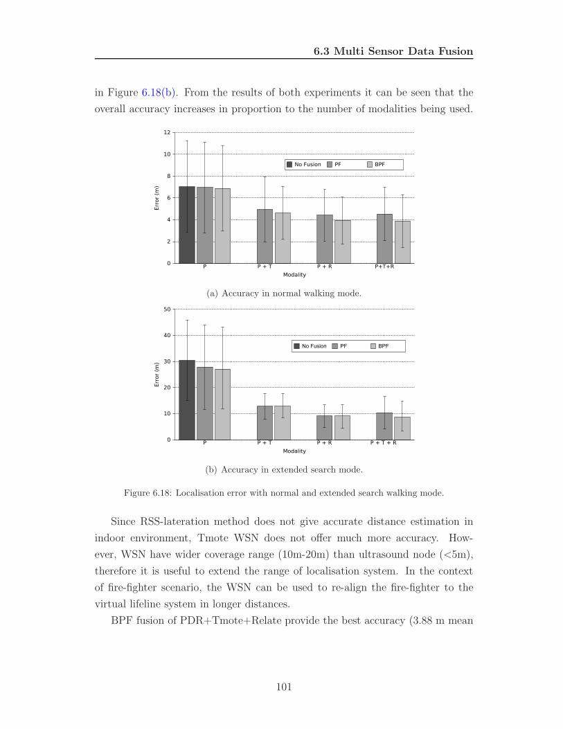
6.3 Multi Sensor Data Fusion
in Figure 6.18(b). From the results of both experiments it can be seen that the
overall accuracy increases in proportion to the number of modalities being used.
P P + T P + R P+T+R
Modality
0
2
4
6
8
10
12
Err
or
(m)
No Fusion PF BPF
(a) Accuracy in normal walking mode.
P P + T P + R P + T + R
Modality
0
10
20
30
40
50
Err
or
(m)
No Fusion PF BPF
(b) Accuracy in extended search mode.
Figure 6.18: Localisation error with normal and extended search walking mode.
Since RSS-lateration method does not give accurate distance estimation in
indoor environment, Tmote WSN does not offer much more accuracy. How-
ever, WSN have wider coverage range (10m-20m) than ultrasound node (<5m),
therefore it is useful to extend the range of localisation system. In the context
of fire-fighter scenario, the WSN can be used to re-align the fire-fighter to the
virtual lifeline system in longer distances.
BPF fusion of PDR+Tmote+Relate provide the best accuracy (3.88 m mean
101
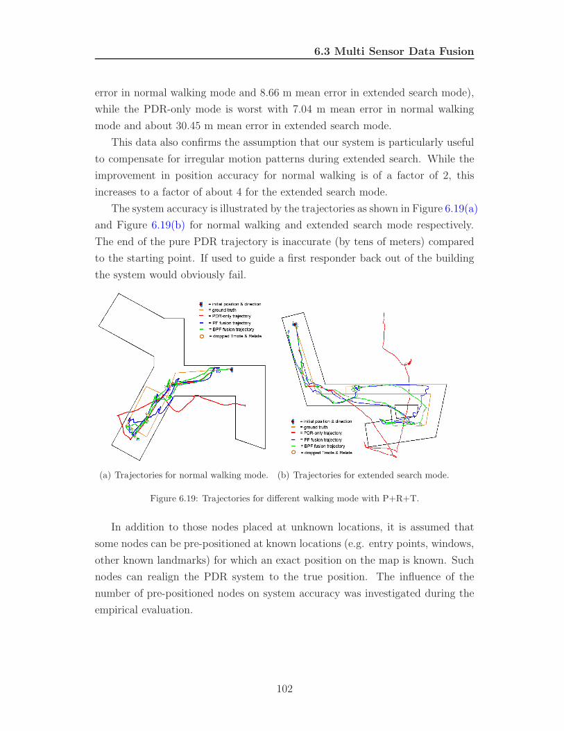
6.3 Multi Sensor Data Fusion
error in normal walking mode and 8.66 m mean error in extended search mode),
while the PDR-only mode is worst with 7.04 m mean error in normal walking
mode and about 30.45 m mean error in extended search mode.
This data also confirms the assumption that our system is particularly useful
to compensate for irregular motion patterns during extended search. While the
improvement in position accuracy for normal walking is of a factor of 2, this
increases to a factor of about 4 for the extended search mode.
The system accuracy is illustrated by the trajectories as shown in Figure 6.19(a)
and Figure 6.19(b) for normal walking and extended search mode respectively.
The end of the pure PDR trajectory is inaccurate (by tens of meters) compared
to the starting point. If used to guide a first responder back out of the building
the system would obviously fail.
(a) Trajectories for normal walking mode. (b) Trajectories for extended search mode.
Figure 6.19: Trajectories for different walking mode with P+R+T.
In addition to those nodes placed at unknown locations, it is assumed that
some nodes can be pre-positioned at known locations (e.g. entry points, windows,
other known landmarks) for which an exact position on the map is known. Such
nodes can realign the PDR system to the true position. The influence of the
number of pre-positioned nodes on system accuracy was investigated during the
empirical evaluation.
102
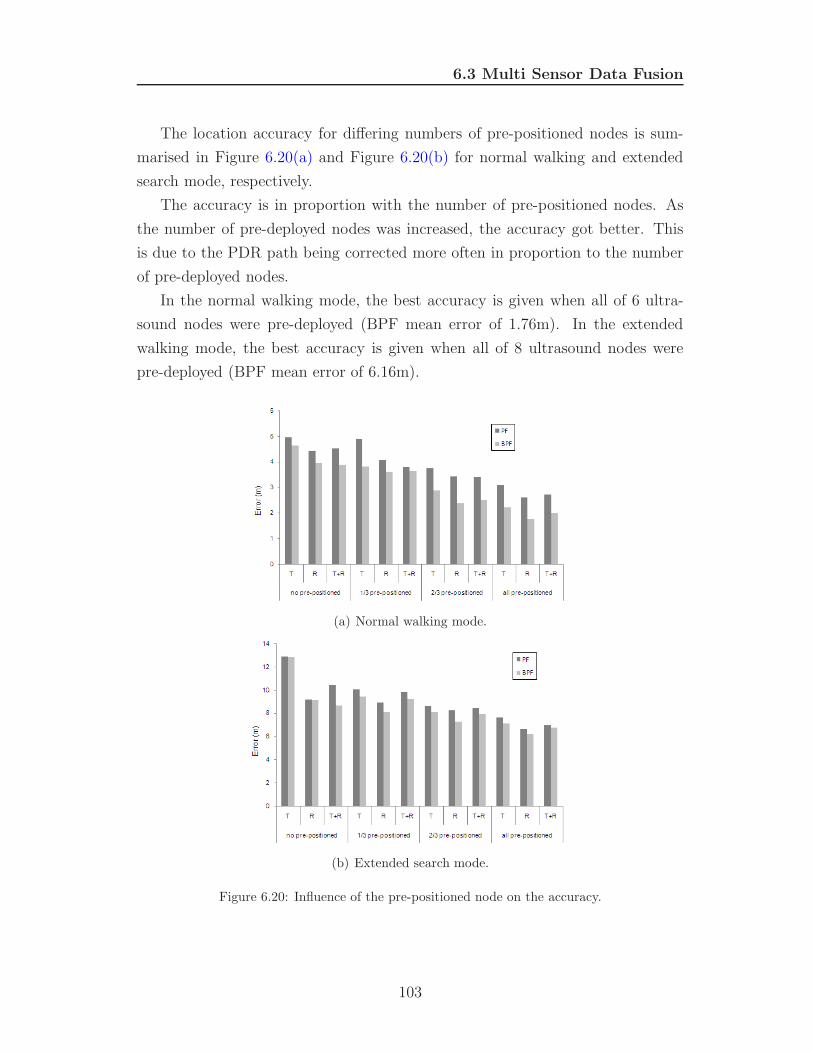
6.3 Multi Sensor Data Fusion
The location accuracy for differing numbers of pre-positioned nodes is sum-
marised in Figure 6.20(a) and Figure 6.20(b) for normal walking and extended
search mode, respectively.
The accuracy is in proportion with the number of pre-positioned nodes. As
the number of pre-deployed nodes was increased, the accuracy got better. This
is due to the PDR path being corrected more often in proportion to the number
of pre-deployed nodes.
In the normal walking mode, the best accuracy is given when all of 6 ultra-
sound nodes were pre-deployed (BPF mean error of 1.76m). In the extended
walking mode, the best accuracy is given when all of 8 ultrasound nodes were
pre-deployed (BPF mean error of 6.16m).
(a) Normal walking mode.
(b) Extended search mode.
Figure 6.20: Influence of the pre-positioned node on the accuracy.
103
6.4 Conclusion
6.4 Conclusion
In this chapter evaluation of the proposed algorithms for improving the accuracy
and usability of the indoor localisation system has been performed. In the first
part (section 6.1), PF, MF and BPF were evaluated and compared with existing
NN and KF algorithms. The best performance was given by the BPF + MF
algorithm which achieved nearly 3 times better accuracy than that obtained for
the NN algorithm.
Typical applications that require 2-3m accuracies can take advantage of this
enhancement. Applications that localises employee in office environment or pa-
tient in a hospital setting is one of the possible implementations.
Furthermore, the influence of the algorithm parameters on localisation accu-
racy was also investigated. These parameters are: the standard deviation σ+ for
the measurement model, the number of attempt for MF and the tail length for
BPF.
Standard deviation σ+ between 4dBm - 5 dBm is recommended for indoor
localisation in an environment similar with office setting (characterised by many
walls, corridors and rooms), such as hospital, campus or apartment. Attempt
value of 8 is suggested since it gives minimum localisation error and only needs
a modest computational power. Based on evaluation of the result, a tail length
of 15-20 is proposed to give the best accuracy.
Section 6.2 which describes evaluation of the algorithm for addressing the
fingerprint usability problem give encouraging results. The self-calibration algo-
rithm was superior to the fingerprint prediction approach. The ability to auto-
matically build and optimise a fingerprint was also demonstrated. It also out-
performs the accuracy of state-of the art methods. Moreover, it has a significantly
lower computation time compared to manually calibrated fingerprint.
Furthermore, the proposed algorithm could be conveniently used for multi
sensor data fusion (section 6.3). Sensor data fusion of WLAN and WSN are im-
plemented when higher accuracy is required. To demonstrate that the algorithm
was also useful for multi sensor data fusion in an emergency scenario, a virtual
lifeline system was proposed. It was used to fuse PDR, ultrasound node and
WSN.
104
6.4 Conclusion
The proposed system of virtual lifeline was proved useful for indoor local-
isation when localisation infrastructure was not available in the environment.
Therefore, the system relied on sensors carried and deployed by the users of the
system on an ad-hoc basis.
It was demonstrated that the implementation of a particle filter, map filtering
and backtracking particle filter significantly enhance the accuracy of the oppor-
tunistic indoor localisation system.
Furthermore, the ability to automatically build and optimised fingerprint, to
improve accuracy and to alleviate cumbersome manual-calibration make the self
calibration algorithm a significant enhancement on the usability of opportunistic
indoor localisation.
It also showed that the particle filter-based multi sensor data fusion is able to
further enhance the accuracy of the opportunistic system.
Therefore, it was demonstrated that the proposed algorithms are able to over-
come the drawbacks of current methods in opportunistic systems. The developed
algorithms are the foundation in achieving an affordable, accurate and usable
opportunistic indoor localisation system. These characteristics enable the large
scale adoption of indoor localisation systems. The proposed algorithms are novel
and become the thesis contribution to enhance the state of the art of opportunistic
systems.
105
Chapter 7
Conclusion
7.1 Summary
The main objectives of this dissertation as set out in section 1.2 are as follows:
1. A comprehensive review of the state of the art of indoor localisation systems,
with a particular focus on highlighting opportunities for an affordable, ac-
curate, and usable opportunistic indoor localisation system.
2. Development and evaluation of a filtering algorithm with a Bayesian ap-
proach to enhance the accuracy of opportunistic indoor localisation.
3. Development and evaluation of a learning data fusion algorithm to enhance
the accuracy and usability of opportunistic indoor localisation.
4. Investigation of the sensor data fusion algorithm between different localisa-
tion technologies and also algorithm implementation in different application
domain.
5. Evaluation and comparison of the developed algorithms against current ap-
proaches with a particular focus on the implementation of opportunistic in-
door localisation.
106
7.1 Summary
Outcomes
The research work documented in this dissertation was performed to achieve the
aforementioned objectives. In the next section, the main contributions of this
work are outlined and the conclusions that can be drawn from the research are
presented.
1. State of the Art of Indoor Localisation
Chapter 2 described current approaches to development of localisation systems.
It was found that utilising RSS of the wireless-communication channel for oppor-
tunistic indoor localisation offers several advantages, such as affordability (since
RSS is virtually free to obtain) and a low technology barrier to implementation
(section 2.1).
WLAN has become the dominant local wireless networking technology. Ac-
cordingly, majority of the opportunistic indoor localisations use RSS of WLAN
as the technology platform of choice.
Section 2.2 focused on current approaches to the opportunistic indoor lo-
calisations. It was found that there are some aspects of current approaches in
opportunistic indoor localisation that need to be addressed with more research;
namely, improvement in the accuracy and usability of the system.
Some algorithms tried to enhance the accuracy of opportunistic indoor lo-
calisations. However, it was found that the proposed methods still have many
disadvantages. Based on the review of the state of the art, the particle filter algo-
rithm had been identified as the most viable method for the opportunistic system.
Therefore, a particle filter-based algorithm was implemented in the opportunistic
indoor localisation.
To address the fingerprinting problem, current methods use indoor propa-
gation modellings or machine learning approaches. However, the proposed so-
lutions still have many shortcomings which restrict them from fully addressing
the problems associated with an opportunistic system. Therefore, this research
constructed novel algorithms for enhancing not only the accuracy but also the
usability of the opportunistic localisation system.
107
7.1 Summary
2. Particle Filter for Localisation
Chapter 3 described the implementation of the most advanced algorithm, the
particle filter, for opportunistic indoor localisation. It was found that the ability
to deal with a non-linear and non-Gaussian system, the suitability for estimation
of dynamic state with large process noise, and the robustness of the algorithm
make particle filter an ideal approach for RSS-based opportunistic system.
Furthermore, novel motion and measurement models were devised to enable
the implementation of particle filter into opportunistic system.
Motion Model
A motion model was developed as a combination from both Brownian movement
and first-order motion models. This model assumed that the kinematic of a target
had random values in it. However, the randomness is constrained by the previous
state (section 3.4).
This approach more accurately reflects the target’s kinematic behaviour in
opportunistic system. It made particles behave more realistic, even in the absence
of motion sensor.
Measurement Model
This research proposed a measurement model which properly considered the phys-
ical characteristics of signal propagation in indoor environments. The measure-
ment model was derived from statistical inference between a fingerprint and RSS
measurements.
Algorithm 3.4 described the steps necessary to obtain a likelihood observation
function. Section 3.5.3 further described a method to obtain intrinsic parameters
of the measurement model.
The devised measurement model leads to a more accurate representation of
the sensor model in the opportunistic system which in turn leads to more accurate
location estimations.
The novel motion and measurement models enable the adoption of a particle
filter into opportunistic indoor localisation. The implementation of a particle
108
7.1 Summary
filter leads into the enhancement of the accuracy of opportunistic indoor locali-
sation.
The limitation of a particle filter is that it needs a relatively high computa-
tional power compared to other methods. Recently, this disadvantage becomes
less apparent because of the continuous development of more powerful hardware.
Implementing a particle filter in resource constrained devices (such as a PDA or
a mobile phone) can be a challenge. However, a client-server architecture allows
one to distribute the majority of computation to a central server.
3. Learning Data Fusion
Chapter 4 presented a learning data fusion algorithm. To improve further the
accuracy, this research examined other information beyond available signal in the
environment, i.e. map information and particle trajectory.
Map filtering was used to fuse map information into the particle filter. More-
over, particle trajectory is fused to refine the state estimation with the backtrack-
ing particle filter algorithm. Both algorithms were devised to further increase the
accuracy of opportunistic systems. Furthermore, with the aim of addressing the
usability problem, a self-calibration algorithm was devised to automatically gen-
erate and calibrate the RSS fingerprint.
The collection of algorithms to enhance the accuracy and usability of an op-
portunistic system is one of the most important contributions of this research.
Map Filtering (MF)
Map information is used to constrain particle motion using the map filtering
algorithm. Fusing the map with the particle filter algorithm is achieved by in-
cluding the constraint rule in the motion model of the particle. The map filtering
algorithm is presented in algorithm 4.1 in section 4.1.2.
The implementation of a particle filter in opportunistic indoor localisation is a
novel approach for opportunistic indoor localisation. It leads to an enhancement
of the accuracy of opportunistic indoor localisation.
109
7.1 Summary
Backtracking Particle Filter (BPF)
BPF is a technique for refining state estimates based on particle trajectory. The
incorporation of the MF technique allowed BPF to exploit long-range geometri-
cal constraints of a map and a long-term likelihood observation function. Algo-
rithm 4.2 describes the steps for BPF algorithm.
The fusion of particle trajectory through backtracking particle filter is one of
the novel contributions of this research. It leads to further enhancement of the
accuracy of an opportunistic system.
The limitation of BPF is that it can only refine past state xt−b. From applica-
tion perspective, the BPF technique can be useful for applications that are toler-
ant to the introduced delay, such as an application that analyses user movement
pattern in an indoor environment. For application that real-time localisation is
a requirement, PF and MF is more appropriate.
Self Calibration Fingerprint
Self-calibration fingerprinting was devised to eliminate the labour-intensive man-
ual calibration and makes the fingerprint adaptive to any change in the system
or environment configuration. The self-calibration algorithm is described in Fig-
ure 4.5 in section 4.3.
This algorithm advances state-of-the-art fingerprinting methods in several key
areas: it removes the necessity to collect initial training data; it elevates the
necessity for placing dedicated RF receivers used for constantly measuring RSS
values; it automatically optimises wall parameter for the propagation model.
The novelty of the algorithm lies in the ability to automatically build and
optimise the fingerprint, and to make the fingerprint adaptive to any change in the
system or environment configuration, thus significantly enhancing the usability
of the opportunistic system.
Self-calibration fingerprinting is one of the most important contributions of
this research.
110
7.1 Summary
4. Multi Sensor Data Fusion
Chapter 5 presented a particle filter-based algorithm for sensor data fusion of
multi-modal localisation technology. The sensor data fusion is investigated to
achieve more fine-grained accuracy of opportunistic indoor localisation.
Fusion of WSN and WLAN was investigated to achieve more fine-grained
accuracy in the context of localisation in the car industry. It was found that RSS
values of WSN gives distinctive measurement probability between fingerprinting
grids. Eventually, it leads to better localisation accuracy when WLAN and WSN
are fused.
Fusion of PDR, ultrasound and WSN was investigated to increase the accuracy
of indoor localisation for fire-fighters. Motion and measurement models of PDR,
ultrasound and WSN were devised to enable the fusion. Fusion for PDR was
implemented by incorporating displacement estimates into the particle motion
model. Novel measurement models based on Gaussian density function were
devised for ultrasound and WSN to enable the fusion.
The fusion of an opportunistic system with different technologies through the
development of sensor-specific probabilistic models is one of the contributions of
this research.
5. Evaluation
Chapter 6 described the evaluation of the proposed algorithms for improving the
accuracy and usability of the indoor localisation system that had been performed.
Evaluation of the algorithms was conducted by means of experiments using a real
test-bed in CIT and Passau University, Germany.
The evaluation showed favourable results. In the first part (section 6.1), PF,
MF and BPF were evaluated and compared with existing NN and KF algo-
rithms. The best performance was given by the BPF + MF algorithm (µ =1.98m
σ =1.11m).
Section 6.2 which describes evaluation of the algorithm for addressing the
fingerprint usability problem gives encouraging results. The self-calibration al-
gorithm significantly provided a better result than the fingerprint prediction ap-
proach. The ability to automatically build and optimise a fingerprint was also
111
7.2 Future Work
demonstrated. It also out-performs the accuracy of state-of the art methods (NN
and KF). Moreover, it has a significantly lower computation time compared to
manually calibrated fingerprint.
Furthermore, the proposed algorithm could be conveniently used for multi
sensor data fusion (section 6.3). Sensor data fusion of WLAN and WSN are im-
plemented when higher accuracy is required. To demonstrate that the algorithm
was also useful for multi sensor data fusion in an emergency scenario, a virtual
lifeline system was proposed. It was used to fuse PDR, ultrasound node and
WSN.
It was demonstrated that the implementation of a particle filter, map filtering
and backtracking particle filter significantly enhance the accuracy of the oppor-
tunistic indoor localisation system.
Furthermore, the ability to automatically build and optimise a fingerprint, to
improve accuracy and to alleviate cumbersome manual-calibration make the self
calibration algorithm is able to significantly enhance the usability of opportunistic
indoor localisation.
It also showed that the particle filter-based multi sensor data fusion is able to
enhance the accuracy of the opportunistic system.
Therefore, it was demonstrated that the proposed algorithms are able to over-
come the drawback of current methods in opportunistic systems. The algorithms
were demonstrated to be able to improve the accuracy and usability of the in-
door localisation system. The proposed algorithms are novel and become thesis
contribution to enhance the state of the art of opportunistic system.
7.2 Future Work
Learning Bayesian Network for the Self-Calibration
As stated in the description of the self-calibration algorithm in section 4.3, opti-
misation of wall parameters of the MWM is performed by a linear method. This
linear optimisation was only applied to a single wall segment at a time, meaning
that adjacent walls did not have an influence, or were not in turn influenced by,
the optimised wall segment.
112
7.3 Conclusion
Consideration of neighbouring or adjacent walls in the overall optimisation
model would potentially produce better optimisation results. This could be
achieved by a learning Bayesian network which describes walls by means of a
probabilistic graphical model and their conditional independences. This model
would allow calculation of interdependencies between wall segments during opti-
misation.
3D Multi-Floor & Multi-Building
Currently, the implementation of an opportunistic localisation system is suit-
able for a 2D single floor. Multi-floor environments are stacked as 2.5D struc-
ture, but extension into 3D multi-floor and multi-building environments would
be highly desirable. The computational requirements for the localisation algo-
rithm and 3D propagation model will increase, but the fundamental PF/BPF
and self-calibration algorithm could easily be extended for this purpose.
Smart-Phone based Opportunistic Localisation
Recent mobile phones, in addition to the GSM interface, have been equipped with
various sensors such as the WLAN interface, GPS, compass and accelerometer.
Using these sensors for opportunistic localisation would be a logical develop-
ment of the present study. The multi-modal sensor data fusion could be easily
re-used. However, the relatively low computational power of the mobile phone
needs to be considered when implementing the algorithm.
7.3 Conclusion
Indoor localisation systems are evolving towards so-called opportunistic localisa-
tion systems. These take advantage of any readily available information in the
environment and a mobile device, such as RSS. Problems inherent in current
approaches to opportunistic localisation that need to be addressed include fur-
ther improvement of the accuracy and usability of the system. In addition, sensor
113
7.3 Conclusion
data fusion capability is overlooked with existing approaches, even though the ac-
curacy of a single-technology platform often cannot satisfy practical application
requirements (see chapter 2 State of the Art).
Hence, development of more advanced algorithms is essential to the wider
adoption of a low-cost, accurate and practical indoor localisation system. This
thesis offers a solution by enhancing the current particle filter approaches for
opportunistic localisation and by constructing a novel algorithm for solving the
usability problem (chapter 3 and 4). Furthermore, the algorithm was able to
become a framework for the sensor data fusion between multi modal localisation
technologies (chapter 5).
To adapt the particle filter algorithm for opportunistic localisation, novel mo-
tion and measurement models were devised. The motion model was an enhance-
ment from both Brownian movement and first-order motion model. This work
also proposed a measurement model which properly considers the physical char-
acteristics of signal propagation in indoor environments (algorithm 3.4). This
evaluation demonstrated that implementation of the particle filter in opportunis-
tic localisation resulted in better localisation accuracy compared to existing con-
ventional algorithms (chapter 6).
The particle filter algorithm was improved further to take advantage of envi-
ronment description and history of RSS measurement. The algorithms used are
called MF and BPF. Implementation of MF and BPF for opportunistic localisa-
tion further improved the accuracy of the localisation system.
Self-calibration fingerprinting was devised to significantly enhance system us-
ability. The evaluation shown in chapter 6 demonstrates that the algorithm can
overcome the problems of manual fingerprint collection enabling automatic gener-
ation and calibration of the RSS fingerprint. The algorithm keeps the fingerprint
up-to-date, thus achieving self-calibration of the localisation system.
In addition, the algorithm can be further utilised for sensor data fusion of
multi-modal localisation technology to achieve more fine-grained accuracy. Fur-
thermore, a data fusion algorithm was implemented in an indoor localisation
system commonly used for first-responders in emergency scenarios. This virtual
lifeline system could be used for indoor localisation in cases where the infrastruc-
ture is not available in the environment.
114

7.3 Conclusion
The work presented in this thesis has demonstrated the ability to address
the problem in perfecting an opportunistic indoor localisation system. The new
algorithm is not only able to enhance the performance of the system, but also
significantly enhanced its usability. This could lead to wider adoption of an
affordable, accurate and usable localisation system.
Eventually, knowledge of physical location could open up a wide range of
possible applications. For example, tracking people and assets, safety and security
or navigating people out of buildings on fire during emergency situations. The
aforementioned applications would help to do things more efficiently, save time,
money and, perhaps, lives.
115
References
[1] M. Weiser, “Some computer science problems in ubiquitous computing,”
Communications of the ACM, 1993.
[2] J. Farrell and M. Barth, The Global Positioning System and Innertial Nav-
igation. McGraw-Hill Professional, 1999.
[3] G. Roussos and V. Kostakos, “RFID in pervasive computing: State-of-the-
art and outlook,” Elsevier Pervasive and Mobile Computing, vol. 5, pp.
110–131, 2009.
[4] J. Fontana, “Recent system applications of short-pulse ultra-wideband
(UWB) technology,” IEEE Transaction on Microwave Theory Technology,
vol. 52, pp. 2087– 2104, 2004.
[5] N. S. Correal, S. Kyperountas, Q. Shi, and M. Welborn, “An ultrawide-
band relative location system,” in Proceedings of the IEEE Conference Ultra
Wideband System Technology, 2003.
[6] B. B. Peterson, C. Kmiecik, R. Hartnett, P. M. Thompson, J. Mendoza, and
H. Nguyen., “Spread spectrum indoor geolocation,” Journal of the Institute
of Navigation, vol. 45, no. 2, pp. 97–102, 1998.
[7] X. Li, K. Pahlavan, M. Latva-aho, and M. Ylianttila, “Comparison of indoor
geolocation methods in DSSS and OFDM wireless LAN,” in Proceedings of
the IEEE VTC, vol. 6, September 2000.
[8] C. Drane, M. Macnaughtan, and C. Scott, “Positioning GSM telephones,”
IEEE Communications Magazine, vol. 36, no. 4, pp. 46–54, April 1998.
116
REFERENCES
[9] A. Bensky, Wireless Positioning: Technologies and Application, ser. GNSS
technology and application series. Artech House Publishers, 2008.
[10] K. J. Krizmant, T. E. Biedkatt, and T. S. Rappaportt, “Wireless position
location: Fundamentals, implementation strategies, and sources of error,”
in Proceedings of the VTC, vol. 2, May 1997.
[11] D. Niculescu and B. Nath, “Ad hoc positioning system (APS) using AOA,”
in Proceedings of the IEEE INFOCOM, 2003.
[12] H. Liu, H. Darabi, P. Banerjee, and J. Liu, “Survey of wireless indoor
positioning techniques and systems,” IEEE Transaction on Systems, Man,
and Cybernetics, vol. 37, no. 6, pp. 1067–1077, November 2007.
[13] A. Kupper, Location Based Services: Fundamentals and Operations. John
Wiley & Sons, 2005.
[14] J. Caffery, Wireless Location in CDMA Cellular Radio Systems. Kluwer
Academic Publishers, 2000.
[15] H. A. Karimi and A. Hammad, Eds., Telegeoinformatics: Location-based
Computing and Services. CRC, 2004.
[16] D. Titterton and J. Weston, Strapdown Inertial Navigation Technology.
IEE, 2005.
[17] S. Beauregard, “Omnidirectional pedestrian navigation for first respon-
ders,” in Proceedings of the 4th WPNC, Hannover, Germany, March 22
2007.
[18] M. Kourogi and T. Kurata, “A method of personal positioning based on
sensor data fusion of wearable camera and self-contained sensors,” in Pro-
ceedings of IEEE MFI, 2003.
[19] H. Aoki, B. Schiele, and A. Pentland, “Realtime personal positioning system
for wearable computers,” in Proceedings of the International Symposium on
Wearable Computing. IEEE Computer Society, 1999, pp. 37–43.
117
REFERENCES
[20] N. Checka and K. Wilson, “Person tracking using audio-video sensor fu-
sion,” 2001, MIT Artificial Intelligence Laboratory, 200 Technology Square,
Cambridge MA, 02139 USA.
[21] M. Kanaan and K. Pahlavan, “A comparison of wireless geolocation algo-
rithms in the indoor environment,” in Proceedings of the IEEE Wireless
Communication Network Conference, 2004.
[22] B. Fang, “Simple solution for hyperbolic and related position fixes,” IEEE
Transaction on Aerospace and Electronic System, vol. 26, pp. 748–753,
September 1990.
[23] A. Goldsmith, Wireless Communication. Cambridge University Press,
2005.
[24] R. Want, A. Hopper, V. Falcao, and J. Gibbons, “The active badge location
system,” ACM Transactions on Information Systems, vol. 10, pp. 91–102,
January 1992.
[25] M. Porreta, P. Nepa, G. Manara, and F. Giannetti, “Location, location,
location,” IEEE Vehicular Technology Magazine, vol. 3, no. 2, pp. 20–29,
June 2008.
[26] (2009, March). [Online]. Available: http://www.ubisense.net
[27] (2009, March). [Online]. Available: http://www.aetherwire.com
[28] (2009, March). [Online]. Available: http://www.timedomain.com
[29] M. Vossiek, L. Wiebking, P. Gulden, J. Wieghardt, C. Hoffmann, and
P. Heide, “Wireless local positioning,” IEEE Microwave Magazine, vol. 4,
pp. 77–86, 2003.
[30] (2009, March). [Online]. Available: http://www.symeo.com/English/
[31] N. Patwari, “Location estimation in sensor network,” Ph.D. dissertation,
University of Michigan, 2005.
118
REFERENCES
[32] K. Romer, “Time synchronization and localization in sensor networks,”
Ph.D. dissertation, ETH Zurich, 2005.
[33] A. Kotanen, M. Hannikainen, H. Leppakoski, and T. D. Hamalainen, “Ex-
periments on local positioning with bluetooth,” in Proceedings of the IEEE
International Conference Infomation Technology, April 2003, pp. 954–958.
[34] J. Hallberg, M. Nilsson, and K. Synnes, “Positioning with bluetooth,” in
Proceedings of the IEEE 10th International Conference on Telecommunica-
tions, 2003.
[35] A. Schwaighofer, M. Grigoras, V. Tresp, and C. Hoffmann, “GPPS: A Gaus-
sian process positioning system for cellular networks,” in NIPS. MIT Press,
2004.
[36] P. Bahl and V. Padmanabhan, “RADAR: An in-building RF-based user lo-
cation and tracking system,” in Proceedings of the IEEE INFOCOM, March
2000, pp. 775–784.
[37] S. Y. Seidel and T. S. Rapport, “914 mhz path loss prediction model for
indoor wireless communications in multi-floored buildings,” IEEE Trans-
action on Antennas & Propagation, vol. 40, pp. 207 – 217, 1992.
[38] K. Lorincz and M. Welsh, “MoteTrack: a robust, decentralized approach
to RF-based location tracking,” Personal Ubiquitous Computing, vol. 11,
no. 6, pp. 489–503, 2007.
[39] A. LaMarca et al., “Place Lab: Device positioning using radio beacons in
the wild,” in Proceedings of the Pervasive, 2005.
[40] R. Battiti, T. L. Nhat, and A.Villani, “Location-aware computing: A neural
network model for determining location in wireless LANs,” University of
Trento, Tech. Rep. DIT-02-0083, February 2002.
[41] A. Kushki, K. N. Plataniotis, and A. N. Venetsanopoulos, “Kernel-based
positioning in wireless local area networks,” IEEE Transaction on Mobile
Computing, vol. 6, no. 6, pp. 689–705, June 2007.
119
REFERENCES
[42] M. Brunato and R. Battiti, “Statistical learning theory for location finger-
printing in wireless LANs,” Elsevier Computer Networks and ISDN Sys-
tems, vol. 47, pp. 825 – 845, April 2005.
[43] S. J. Pan, V. W. Zheng, Q. Yang, and D. H. Hu, “Transfer learning for
WiFi-based indoor localization,” in Proceedings of the AAAI-08 Workshop
on Transfer Learning for Complex Task, 2008.
[44] M. Youssef, A. Agrawala, and A. U. Shankar, “WLAN location determi-
nation via clustering and probability distributions,” in Proceedings of the
IEEE PerCom, 2003.
[45] M. Youssef and A. K. Agrawala, “Handling samples correlation in the Horus
system,” in Proceedings of the IEEE INFOCOM, 2004.
[46] M. B. Kjærgaard, “A taxonomy for radio location fingerprinting,” LCNS,
vol. 4718, pp. 139–156, 2007.
[47] S. Thrun, “Robotic mapping: A survey,” in Exploring Artificial Intelligence
in the New Millenium. Morgan Kaufmann, 2002.
[48] D. Simon, Optimal State Estimation: Kalman, H Infinity, and Nonlinear
Approaches. Wiley-Interscience, 2006.
[49] D. Fox, J. Hightowerand, L. Liao, D. Schulz, and G. Borriello, “Bayesian
filtering for location estimation,” IEEE Pervasive Computing, vol. 02, no. 3,
pp. 24–33, 2003.
[50] N. Sirola, “Mathematical methods for personal positioning and navigation,”
Ph.D. dissertation, Tampere University of Technology, 2007.
[51] S. Thrun, D. Fox, W. Burgard, and F. Dellaert, “Robust Monte Carlo
localization for mobile robots,” Artificial Intelligence, vol. 128, pp. 99–141,
2001.
[52] M. Heidari, “A testbed for real-time performance evaluation of RSS-based
indoor geolocation systems in laboratory environment,” Master’s thesis,
Worcester Polytechnic Institute, 2005.
120
REFERENCES
[53] (2009, March). [Online]. Available: http://www.ekahau.com/
[54] D. L. Hall and J. Llinas, “An introduction to multisensor data fusion,”
Proceedings of the IEEE ISCAS, vol. 85, no. 1, January 1998.
[55] D. L. Hall and J. Llinas, Handbook on Multisensor Data Fusion. CRC,
2001.
[56] J. Hightower and G. Borriello, “Particle filters for location estimation in
ubiquitous computing: A case study,” in Proceedings of the 6th Ubicomp,
September 2004.
[57] J. Castellanos, J. Neira, and J. Tards, “Multisensor fusion for simultane-
ous localization and map building,” IEEE Transactions on Robotics and
Automation, vol. 17, pp. 908–914, 2001.
[58] Widyawan, M. Klepal, and D. Pesch, “Influence of predicted and mea-
sured fingerprint on the accuracy of RSSI-based indoor location systems,”
in Proceedings of the 4th IEEE WPNC 2007, Hannover, Germany, March
2007.
[59] A. Narzullaev, Y. Park, and H. Jung, “Accurate signal strength predic-
tion based positioning for indoor WLAN systems,” in Proceedings of the
IEEE/ION Position, Location and Navigation Symposium, 2008.
[60] M. Lott and I. Forkel, “A multi-wall-and-floor model for indoor radio prop-
agation,” in Proceedings of the IEEE VTC Spring, 2001.
[61] M. Klepal, “Novel approach to indoor electromagnetic wave propagation
modelling,” Ph.D. dissertation, Czech Technical University, 2003.
[62] X. Chai and Q. Yang, “Reducing the calibration effort for probabilistic in-
door location estimation,” IEEE Transaction on Mobile Computing, vol. 6,
pp. 649–662, 2007.
[63] Z. Xiang, S. Song, J. Chen, H. Wang, J. Huang, and X. Gao, “A wireless
LAN-based indoor positioning technology,” IBM Journal of Research and
Development, vol. 48, no. 5/6, pp. 617–626, 2004.
121
REFERENCES
[64] J. Yin, Q. Yang, and L. Ni, “Learning adaptive temporal radio maps for
signal-strength-based location estimation,” IEEE Transactions on Mobile
Computing, vol. 7, pp. 869–883, 2007.
[65] S. Thrun, W. Burgard, and D. Fox, Probabilistic Robotics (Intelligent
Robotics and Autonomous Agents). The MIT Press, September 2005.
[66] D. P. Bertsekas and J. N. Tsikilis, Introduction To Probability. Athena
Scientific, 2002.
[67] M. S. Arulampalam, S. Maskell, N. Gordon, and T. Clapp, “A tutorial on
particle filters for online nonlinear/non-Gaussian Bayesian tracking,” IEEE
Transaction on Signal Processing, vol. 50, no. 2, pp. 174–188, 2002.
[68] B. D. O. Anderson and J. B. Moore, Optimal Filtering. Dover Publications
Inc., 2005.
[69] A. Papoulis, Probability, Random Variables, and Stochastic Processes.
McGraw-Hill Companies, 1984.
[70] P. S. Maybeck, Stochastic Models, Estimation and Control. Academic
Press, 1982.
[71] R. E. Kalman, “A new approach to linear filtering and prediction problems,”
Transactions of the ASME Journal of Basic Engineering, vol. 82, pp. 35–
45, 1960.
[72] R. Kalman, “New methods in Wiener fltering theory,” in Proceedings of the
Symposium of Application Random Function Theory and Probability, 1963.
[73] A. Doucet, N. de Freitas, and N. Gordon, Eds., Sequential Monte Carlo
Methods in Practice, 1st ed. New York: Springer, June 2001.
[74] B. Ristic, S. Arumpalampam, and N. Gordon, Beyond the Kalman Fil-
ter: Particle Filters for Tracking Applications. Artech House Publishers,
February 2004.
122
REFERENCES
[75] N. J. Gordon, D. J. Salmond, and A. F. M. Smith, “Novel approach
to nonlinear/non-Gaussian Bayesian state estimation,” IEE Proceedings F
Radar and Signal Processing, vol. 140, pp. 107–113, 1993.
[76] J. Maccormick and A. Blake, “A probabilistic exclusion principle for track-
ing multiple objects,” in International Journal of Computer Vision, 1999,
pp. 572–578.
[77] K. Kanazawa, D. Koller, and S. Russell, “Stochastic simulation algorithms
for dynamic probabilistic networks,” in Proceedings of the Eleventh Annual
Conference on Uncertainty AI, 1995.
[78] J. S. Liu and R. Chen, “Sequential Monte Carlo methods for dynamic
systems,” Journal of the American Statistical Association, vol. 93, pp. 1032–
1044, 1998.
[79] A. Doucet, S. Godsill, and C. Andrieu, “On sequential Monte Carlo sam-
pling methods for Bayesian filtering,” Statistics and Computing, vol. 10,
pp. 197–208, 2000.
[80] G. Kitagawa, “Monte Carlo filter and smoother for non-Gaussian non-linear
state space model,” Journal of Computational and Graphical Statistics,
vol. 5, pp. 1–25, 1996.
[81] S. Godsill, A. Doucet, and M. West, “Methodology for Monte Carlo smooth-
ing with application to time-varying autoregressions,” in Proocedings of the
International Symposium Frontiers Time Series Modeling, 2000.
[82] S. T. M. Montemerlo and W. Whittaker, “Conditional particle filters for
simultaneous mobile robot localization and people-tracking,” in Proceedings
of the IEEE ICRA, 2002.
[83] E. Meier and F. Ade, “Using the condensation algorithm to implement
tracking for mobile robots,” in Proceedings of the Eurobot, 1999.
[84] A. Bruce, “Better motion prediction for people-tracking,” in Proceedings of
ICRA 2004, 2004.
123
REFERENCES
[85] A. E. Chapman, Biomechanical Analysis of Fundamental Human Move-
ment. Human Kinetics Europe Ltd, 2008.
[86] F. Evennou and F. Marx, “Advanced integration of WiFi and inertial nav-
igation systems for indoor mobile positioning,” EURASIP Journal on Ap-
plied Signal Processing, vol. 2006, pp. 1–11, January 2006.
[87] H. Wang, H. Lenz, A. Szabo, J. Bamberger, and W. D. Hanebeck, “WLAN-
based pedestrian tracking using particle filters and low-cost MEMS sen-
sors,” in Proceedings of the IEEE WPNC’07, 2007.
[88] S. R. Saunders and A. Aragon, Antennas and Propagation for Wireless
Communication Systems, 2nd ed. Wiley & Sons, May 2007.
[89] R. Bansal, Ed., Handbook of Engineering Electromagnetics. CRC, 2004.
[90] M. Klepal, R. Mathur, A. McGibney, and D. Pesch, “Influence of people
shadowing on optimal deployment of WLAN access points,” in Proceedings
of the IEEE VTC, 2004.
[91] A. Alouani and W. Blair, “Use of a kinematic constraint in tracking con-
stant speed, maneuvering targets,” IEEE Transactions on Automatic Con-
trol, vol. 38, pp. 1107–1111, 1993.
[92] N. Svenzen, “Real time implementation of map aided positioning using a
Bayesian approach,” Master’s thesis, Linkoping University, 2002.
[93] S. Oh, S. Tariq, B. Walker, and F. Dellaert, “Map-based priors for local-
ization,” in Proocedings of the IROS, 2004.
[94] H. Choset, “Sensor based motion planning: The hierarchical generalized
Voronoi graph.” Ph.D. dissertation, California Insititute of Technology,
1996.
[95] COST Telecommunications, COST231 Final Report, Digital Mobile Radio:
COST231 View on the Evolution towards 3rd Generation Systems. Brussel:
European Commission/COST Telecommunications, 1998.
124
REFERENCES
[96] R. L. Kruse and A. Ryba, Data Structures and Program Design in C++.
Prentice Hall, 1998.
[97] E. Kreyszig, Advanced Engineering Mathematics. John Wiley & Sons,
1999.
[98] A. Bjorg, Numerical methods for Least Square Problems. Siam, 1996.
[99] 802.15.4-2006 Part 15.4: Wireless MAC and PHY specifications for Low
Rate Wireless Personal Area Networks (LR-WPANS), IEEE Std.
[100] E. Foxlin, “Pedestrian tracking with shoe-mounted inertial sensors,” Com-
puter Graphics and Applications, IEEE, vol. 25, no. 6, pp. 38–46, 2005.
[101] K. F. Stirling, R. and G. Lachapelle, “Evaluation of a new method of head-
ing estimation for pedestrian dead reckoning using shoe mounted sensors,”
Journal of Navigation, vol. 58, no. 1, pp. 31 – 45, 2005.
[102] F. Cavallo, A. Sabatini, and V. Genovese, “A step toward GPS/INS per-
sonal navigation systems: Real-time assessment of gait by foot inertial sens-
ing,” in Proceedings of the IEEE IROS, Edmonton, Canada, August 2005,
pp. 1187 – 1191.
[103] C. Fischer, K. Muthukrishnan, M. Hazas, and H. Gellersen, “Ultrasound-
aided pedestrian dead reckoning for indoor navigation,” in Proceedings of
the MELT, California, September 2008.
[104] M. Hazas, C. Kray, H. Gellersen, H. Agbota, G. Kortuem, and A. Krohn,
“A relative positioning system for co-located mobile devices,” in Proceedings
of the 3rd MobiSys. New York, NY, USA: ACM Press, 2005, pp. 177–190.
[105] S. Beauregard, Widyawan, and M. Klepal, “Indoor PDR performance
enhancement using minimal map information and particle filters,” in Pro-
ceedings of the IEEE/ION PLAN, Monterey, California, May 2008.
[106] M. Klann et al., “LifeNet: an ad-hoc sensor network and wearable system to
provide firefighters with navigation support,” Proceedings of the UbiComp:
Demos Extended Abstracts, 2007.
125
REFERENCES
[107] O. Woodman and R. Harle, “Pedestrian localisation for indoor environ-
ments,” in Proceedings of the 10th UbiComp. New York, NY, USA: ACM,
2008, pp. 114–123.
[108] L. E. Miller, “Indoor navigation for first responders: A feasibility study,”
Wireless Communication Technologies Group, Advanced Networking Tech-
nologies Devision, Information Technology Laboratory, National Institute
of Standards and Technology, Tech. Rep., February 10 2006.
[109] V. Amendolare, D. Cyganski, R. J. Duckworth, S. Makarov, J. Coyne,
H. Daempfling, and B. Woodacre, “WPI precision personnel locator sys-
tem: Inertial navigation supplementation,” in Proceedings of the IEEE/ION
PLAN, Monterey, California, May 2008.
126