Learning Disjunctions of Predicates - ddana.cswp.cs ... · LEARNING DISJUNCTIONS OF PREDICATES 2. The Model and Class Let Fbe a ﬁnite set of boolean functions over a domain X (possibly

Proceedings of Machine Learning Research vol 65:1–23, 2017

Learning Disjunctions of Predicates

Nader H. Bshouty [email protected]

Dana Drachsler-Cohen [email protected]

Martin Vechev [email protected] Zurich

Eran Yahav [email protected]

Technion

AbstractLetF be a set of boolean functions. We present an algorithm for learningF∨ := {∨f∈Sf | S ⊆ F}from membership queries. Our algorithm asks at most |F| ·OPT(F∨) membership queries whereOPT(F∨) is the minimum worst case number of membership queries for learning F∨. When F isa set of halfspaces over a constant dimension space or a set of variable inequalities, our algorithmruns in polynomial time.

The problem we address has practical importance in the field of program synthesis, where thegoal is to synthesize a program that meets some requirements. Program synthesis has becomepopular especially in settings aiming to help end users. In such settings, the requirements are notprovided upfront and the synthesizer can only learn them by posing membership queries to theend user. Our work enables such synthesizers to learn the exact requirements while bounding thenumber of membership queries.

1. Introduction

Learning from membership queries (Angluin, 1988) has flourished due to its many applications ingroup testing (Du and Hwang, 2000, 2006), blood testing (Dorfman, 1943), chemical leak testing,chemical reactions (Angluin and Chen, 2008), electrical short detection, codes, multi-access chan-nel communications (Biglieri and Gyrfi, 2007), molecular biology, VLSI testing, AIDS screening,whole-genome shotgun sequencing (Alon et al., 2002), DNA physical mapping (Grebinski and Ku-cherov, 1998) and game theory (Pelc, 2002). For a list of many other applications, see Du andHwang (2000); Ngo and Du (2000); Bonis et al. (2005); Du and Hwang (2006); Cicalese (2013);Biglieri and Gyrfi (2007). Many of the new applications present new models and new problems.One of these is programming by example (PBE), a popular setting of program synthesis (Polo-zov and Gulwani, 2015; Barowy et al., 2015; Le and Gulwani, 2014; Gulwani, 2011; Jha et al.,2010). PBE has gained popularity because it enables end users to describe their intent to a programsynthesizer via the intuitive means of input–output examples. The common setting of PBE is tosynthesize a program based on a typically small set of user-provided examples, which are often anunder-specification of the target program (Polozov and Gulwani, 2015; Barowy et al., 2015; Le andGulwani, 2014; Gulwani, 2011). As a result, the synthesized program is not guaranteed to fullycapture the user’s intent. Another (less popular) PBE approach is to limit the program space to a

cchar∞3 2017 N.H. Bshouty, D. Drachsler-Cohen, M. Vechev & E. Yahav.

BSHOUTY DRACHSLER-COHEN VECHEV YAHAV

small (finite) set of programs and ask the user membership queries while there are non-equivalentprograms in the search space (Jha et al., 2010). A natural question is whether one can do betterthan the latter approach without sacrificing the correctness guaranteed by the former approach. Inthis paper, we answer this question for a class of specifications (i.e., formulas) that captures a widerange of programs.

We study the problem of learning a disjunctive (or dually, a conjunctive) formula describing theuser intent through membership queries. To capture a wide range of program specifications, theformulas are over arbitrary, predefined predicates. In our setting, the end user is the teacher thatcan answer membership queries. This work enables PBE synthesizers to guarantee to the user thatthey have synthesized the correct program, while bounding the number of membership queries theypose, thus reducing the burden on the user.

More formally, let F be a set of predicates (i.e., boolean functions). Our goal is to learn theclass F∨ of any disjunction of predicates in F . We present a learning algorithm SPEX, which learnsany function in F∨ with polynomially many queries. We then show that given some computationalcomplexity conditions on the set of predicates, SPEX runs in polynomial time.

We demonstrate the above on two classes. The first is the class of disjunctions (or conjunctions,whose learning is the dual problem) over any set H of halfspaces over a constant dimension. For thisclass, we show that SPEX runs in polynomial time. In particular, this shows that learning any convexpolytope over a constant dimension when the sides are from a given set H can be done in polynomialtime. For the case where the dimension is not constant, we show that learning this class impliesP=NP. We note that there are other applications for learning halfspaces; for example, Hegedus(1995); Zolotykh and Shevchenko (1995); Abboud et al. (1999); Abasi et al. (2014).

The second class we consider is conjunctions over F , where F is the set of variable inequalities,i.e., predicates of the form [xi > xj ] over n variables. If the set is acyclic (∧F 6= 0), we show thatlearning can be done in polynomial time. If the set is cyclic (∧F = 0), we show that learning isequivalent to the problem of enumerating all the maximal acyclic subgraphs of a directed graph,which is still an open problem (Acua et al., 2012; Borassi et al., 2013; Wasa, 2016).

The second class has practical importance because it consists of formulas that can be usedto describe time-series charts. Time charts are used in many domains including financial analy-sis (Bulkowski, 2005), medicine (Chuah and Fu, 2007), and seismology (Morales-Esteban et al.,2010). Experts use these charts to predict important events (e.g., trend changes in a stock price)by looking for patterns in the charts. A lot of research has focused on common patterns and manyplatforms enable these experts to write a program that upon detecting a specific pattern alerts theuser (e.g., some platforms for finance analysts are MetaTrader, MetaStock, Amibroker). Unfortu-nately, writing programs is a complex task for these experts, as they are not programmers. To helpsuch experts, we integrated SPEX in a synthesizer that interacts with a user to learn a pattern (i.e., aconjunctive formula over variable inequalities). SPEX enables the synthesizer to guarantee that thesynthesized program captures the user intent, while interacting with him only through membershipqueries that are visualized in charts.

The paper is organized as follows. Section 2 describes the model and class we consider.Section 3 provides the main definitions we require for the algorithm. Section 4 presents the SPEXalgorithm, discusses its complexity, and describes conditions under which SPEX is polynomial.Sections 5 and 6 discuss the two classes we consider: halfspaces and variable inequalities. Finally,Section 7 shows the practical application of SPEX in program synthesis.

2

http://www.metaquotes.net/en/metatrader5

http://www.metastock.com/

http://amibroker.com/

LEARNING DISJUNCTIONS OF PREDICATES

2. The Model and Class

Let F be a finite set of boolean functions over a domain X (possibly infinite). We consider the classof functions F∨ := {∨f∈Sf | S ⊆ F}. Our model assumes a teacher that has a target functionF ∈ F∨ and a learner that knowsF but not the target function. The teacher can answer membershipqueries for the target function – that is, given x ∈ X (from the learner), the teacher returns F (x).The goal of the learner (the learning algorithm) is to find the target function with a minimum numberof membership queries.

Notations Following are a few notations used throughout the paper. OPT(F∨) denotes the mi-nimum worst case number of membership queries required to learn a function F in F∨. Gi-ven F ∈ F∨, we denote by S(F ) the set that consists of all the functions in F . Formally,we define S(F ) = S, where S is the unique subset of F such that F =

∨f∈S f . For exam-

ple, S(f1 ∨ f2) = {f1, f2}. From this, it immediately follows that F1 ≡ F2 if and only ifS(F1) = S(F2). For a set of functions S ⊆ F , we denote ∨S := ∨f∈Sf . Lastly, [S(x)] de-notes the boolean value of a logical statement. Namely, given a statement S(x) : X → {T, F} witha free variable x, its boolean function [S(x)] : X → {0, 1} is defined as [S(x)] = 1 if S(x) = T ,and [S(x)] = 0 otherwise. For example, [x ≥ 2] = 1 if and only if the interpretation of x is greaterthan 2.

3. Definitions and Preliminary Results

In this section, we provide the definitions used in this paper and show preliminary results. We beginby defining an equivalence relation over the set of disjunctions and defining the representativesof the equivalence classes. Thereafter, we define a partial order over the disjunctions and relatednotions (descendant, ascendant, and lowest/greatest common descendant/ascendant). We completethis section with the notion of a witness, which is central to our algorithm.

3.1. An Equivalence Relation Over F∨In this section, we present an equivalence relation over F∨ and define the representatives of theequivalence classes. This enables us in later sections to focus on the representative elements fromF∨. Let F be a set of boolean functions over the domain X . The equivalence relation = over F∨ isdefined as follows: two disjunctions F1, F2 ∈ F∨ are equivalent (F1 = F2) if F1 is logically equalto F2. In other words, they represent the same function (from X to {0, 1}). We write F1 ≡ F2 todenote that F1 and F2 are identical; that is, they have the same representation. For example, considerf1, f2 : {0, 1} → {0, 1} where f1(x) = 1 and f2(x) = x. Then, f1 ∨ f2 = f1 but f1 ∨ f2 6≡ f1.

We denote by F∗∨ the set of equivalence classes of = and write each equivalence class as [F ],where F ∈ F∨. Notice that if [F1] = [F2], then [F1 ∨ F2] = [F1] = [F2]. Therefore, for every [F ],we can choose the representative element to be GF := ∨F ′∈SF ′ where S ⊆ F is the maximum sizeset that satisfies ∨S = F . We denote by G(F∨) the set of all representative elements. Accordingly,G(F∨) = {GF | F ∈ F∨}. As an example, consider the set F consisting of four functionsf11, f12, f21, f22 : {1, 2}2 → {0, 1} where fij(x1, x2) = [xi ≥ j]. There are 24 = 16 elements inRay2

2 := F∨ and five representative functions in G(F∨): G(F∨) = {f11∨f12∨f21∨f22, f12∨f22,f12, f22, 0} (where 0 is the zero function).

The below listed facts follow immediately from the above definitions:

3


Lemma 1 Let F be a set of boolean functions. Then,1. The number of logically non-equivalent boolean functions in F∨ is |G(F∨)|.2. For every F ∈ F∨, GF = F .3. For every G ∈ G(F∨) and f ∈ F\S(G), G ∨ f 6= G.4. For every F ∈ F∨, ∨S(F ) ≡ F .5. If G1, G2 ∈ G(F∨), then G1 = G2 if and only if G1 ≡ G2.

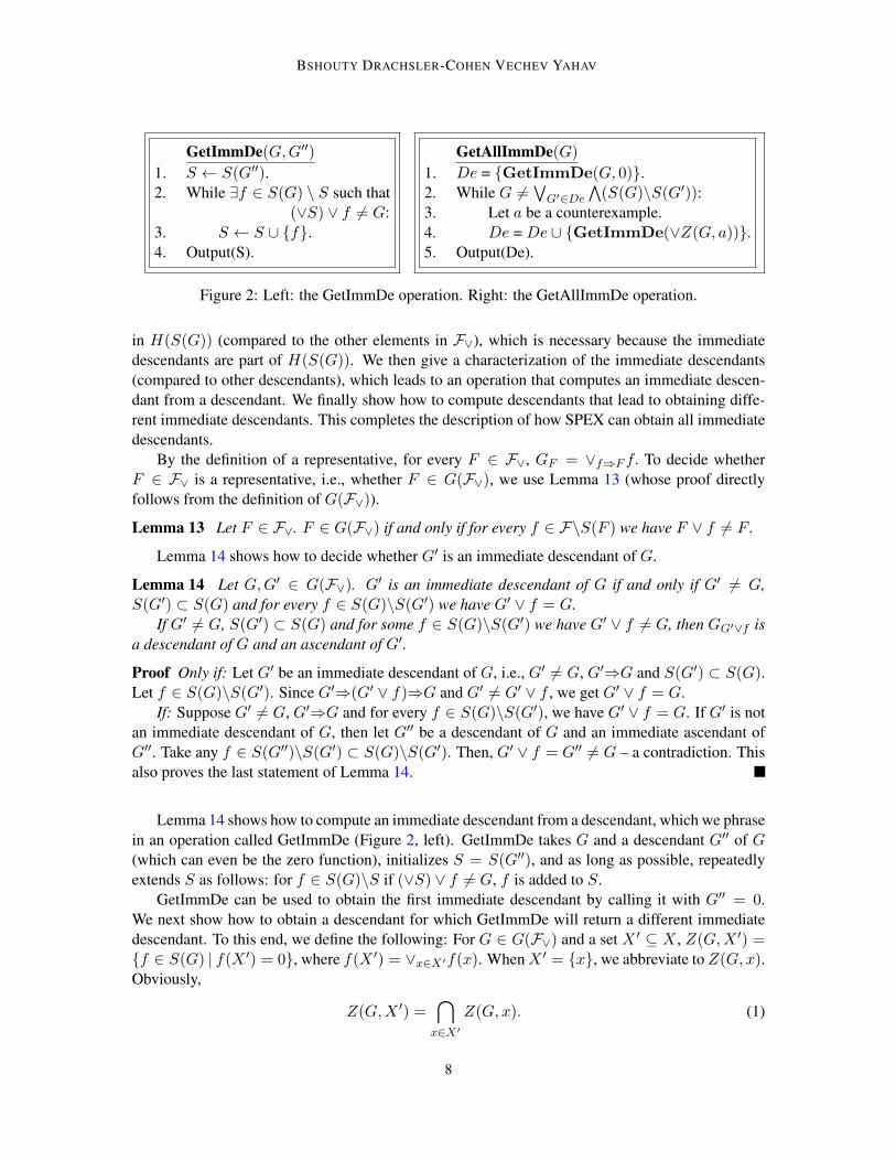
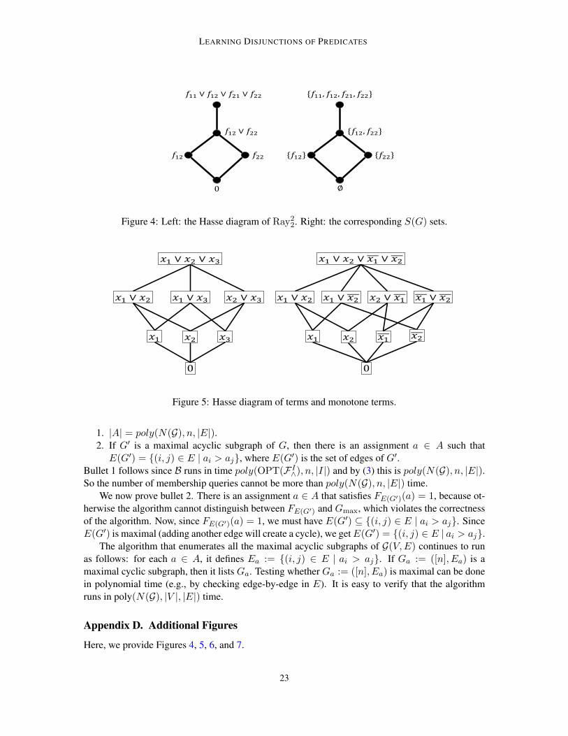
3.2. A Partial Order Over F∨In this section, we define a partial order over F∨ and present related definitions. The partial or-der, denoted by ⇒, is defined as follows: F1⇒F2 if F1 logically implies F2. Consider the Hassediagram H(F∨) of G(F∨) for this partial order. The maximum (top) element in the diagram isGmax := ∨f∈F f . The minimum (bottom) element is Gmin := ∨f∈Øf , i.e., the zero function.Figure 4 shows an illustration of the Hasse diagram of Ray2

2 (from Section 3.1). Figures 5 and 6show other examples of Hasse diagrams: Figure 5 shows the Hasse diagram of boolean variables,while Figure 6 shows an example that extends the example of Ray2

2.In a Hasse diagram, G1 is a descendant (resp., ascendent) of G2 if there is a (nonempty) do-

wnward path from G2 to G1 (resp., from G1 to G2), i.e., G1⇒G2 (resp., G2⇒G1) and G1 6= G2.G1 is an immediate descendant of G2 in H(F∨) if G1⇒G2, G1 6= G2 and there is no G such thatG 6= G1, G 6= G2 and G1⇒G⇒G2. G1 is an immediate ascendant of G2 if G2 is an immediatedescendant of G1. We now show (all proofs for this section appear in Appendix B):

Lemma 2 Let G1 be an immediate descendant of G2 and F ∈ F∨. If G1⇒F⇒G2, then G1 = For G2 = F .

We denote by De(G) and As(G) the sets of all the immediate descendants and immediate as-cendants of G, respectively. We further denote by DE(G) and AS(G) the sets of all G’s des-cendants and ascendants, respectively. For G1 and G2, we define their lowest common ascendent(resp., greatest common descendant) G = lca(G1, G2) (resp., G = gcd(G1, G2)) to be the bool-ean function G ∈ G(F∨) – that is, the minimum (resp., maximum) element in AS(G1) ∩ AS(G2)(resp., DE(G1) ∩DE(G2)). Therefore, we can show Lemma 3. Lemma 3 abbreviates (G1⇒G andG2⇒G) to G1, G2⇒G and (G⇒G1 and G⇒G2) to G⇒G1, G2.

Lemma 3 Let G1, G2 ∈ G(F∨) and F ∈ F∨.1. If G1, G2⇒F⇒lca(G1, G2), then F = lca(G1, G2).2. If gcd(G1, G2)⇒F⇒G1, G2, then F = gcd(G1, G2).

Lemma 3 leads us to Lemma 4:

Lemma 4 Let G1, G2 ∈ G(F∨). Then, lca(G1, G2) = G1 ∨G2.In particular, if G1, G2 are two distinct immediate descendants of G, then G1 ∨G2 = G.

Note that this does not imply that S(G1 ∨G2) = S(G1) ∪ S(G2) = S(lca(G1, G2)). In particular,G1 ∨G2 is not necessarily in G(F∨); see, for example, Figure 5 (right).

Lemma 5 follows from the fact that if G1 is a descendant of G2, then G1⇒G2, and therefore,G1 ∨G2 = G2.

Lemma 5 If G1 is a descendant of G2, then S(G1) ( S(G2).

4


Lemma 5 enables us to show the following.

Lemma 6 Let G1, G2 ∈ G(F∨). Then, S(G1) ∩ S(G2) = S(gcd(G1, G2)).In particular, if G1, G2 ∈ G(F∨), then ∨(S(G1) ∩ S(G2)) ∈ G(F∨).Also, if G1, G2 are two distinct immediate ascendants of G, then S(G1) ∩ S(G2) = S(G).

Note that this does not imply that G1 ∧G2 = gcd(G1, G2); see, for example, Figure 5 (right).

3.3. Witnesses

Finally, we define the term witness. Let G1 and G2 be elements in G(F∨). An element a ∈ X is awitness for G1 and G2 if G1(a) 6= G2(a). We now show two central lemmas.

Lemma 7 Let G1 be an immediate descendant of G2. If a ∈ X is a witness for G1 and G2, then:1. G1(a) = 0 and G2(a) = 1.2. For every f ∈ S(G1), f(a) = 0.3. For every f ∈ S(G2)\S(G1), f(a) = 1.

Proof Since G1⇒G2, it must be that G2(a) = 1 and G1(a) = 0. Namely, for every f ∈ S(G1),f(a) = 0. Let f ∈ S(G2)\S(G1). Consider F = G1 ∨ f . By bullet 3 in Lemma 1, F 6= G1. SinceG1⇒F⇒G2, by Lemma 2, F = G2. Therefore, f(a) = G1(a) ∨ f(a) = F (a) = G2(a) = 1.

Lemma 8 Let De(G) = {G1, G2, . . . , Gt} be the set of immediate descendants of G. If a is awitness for G1 and G, then a is not a witness for Gi and G for all i > 1. That is, G1(a) = 0,G(a) = 1, and G2(1) = · · · = Gt(a) = 1.

Proof By Lemma 7, G(a) = 1 and G1(a) = 0. By Lemma 4, for any Gi, i ≥ 2, we haveG = G1 ∨Gi. Therefore, 1 = G(a) = G1(a) ∨Gi(a) = Gi(a).

4. The Algorithm

In this section, we present our algorithm to learn a target disjunction over F , called SPEX (short forspecifications from examples). Our algorithm relies on the following results.

Lemma 9 Let G′ be an immediate descendant of G, a ∈ X be a witness for G and G′, and G′′ bea descendant of G.

1. If G′′(a)=0, G′′ is a descendant of G′ or equal to G′. In particular, S(G′′) ⊆ S(G′).2. If G′′(a)=1, G′′ is neither a descendant of G′ nor equal to G′. In particular, S(G′′) 6⊂ S(G′).

Proof Since G′′ is a descendant of G, we have S(G′′) ( S(G). By Lemma 7, for every f ∈ S(G′),we have f(a) = 0, and for every f ∈ S(G)\S(G′), we have f(a) = 1. Thus, if G′′(a) = 0, thenno f ∈ S(G)\S(G′) is in S(G′′) (otherwise, G′′(a) = 1). Therefore, S(G′′) ⊆ S(G′) and G′′

is a descendant of G′ or equal to G′. Otherwise, if G′′(a) = 1 , then since G′(a) = 0, for everydescendant G0 of G′ we have G0(a) = 0 and thus G′′ is neither a descendant of G′ nor equal to G′.

5


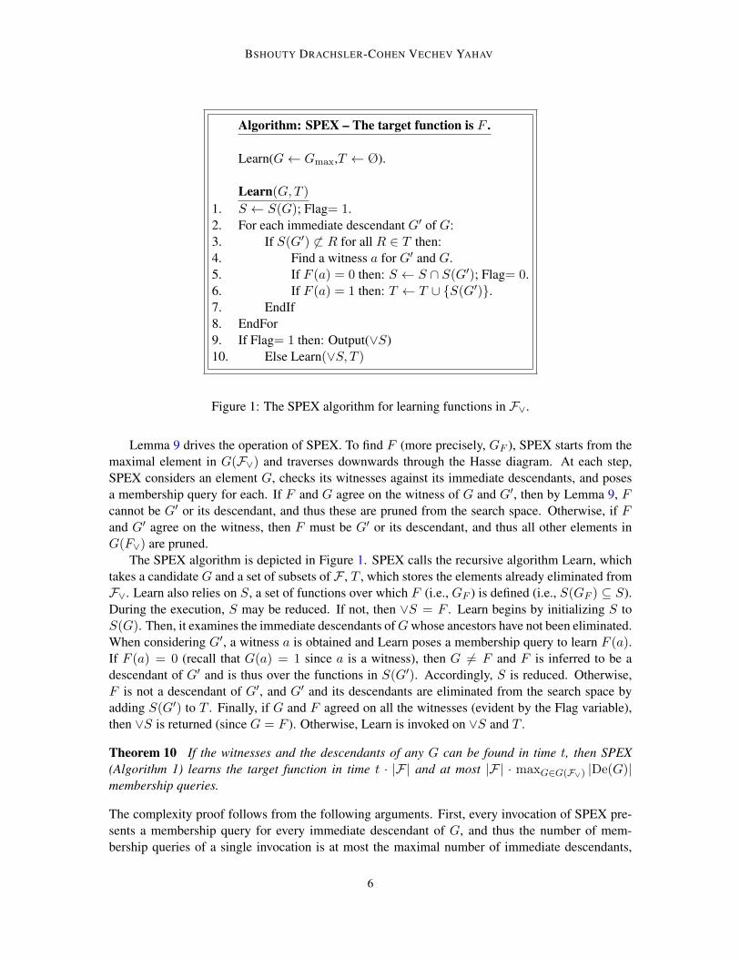
Algorithm: SPEX – The target function is F .

Learn(G← Gmax,T ← Ø).

Learn(G,T )

1. S ← S(G); Flag= 1.2. For each immediate descendant G′ of G:3. If S(G′) 6⊂ R for all R ∈ T then:4. Find a witness a for G′ and G.5. If F (a) = 0 then: S ← S ∩ S(G′); Flag= 0.6. If F (a) = 1 then: T ← T ∪ {S(G′)}.7. EndIf8. EndFor9. If Flag= 1 then: Output(∨S)10. Else Learn(∨S, T )

Figure 1: The SPEX algorithm for learning functions in F∨.

Lemma 9 drives the operation of SPEX. To find F (more precisely, GF ), SPEX starts from themaximal element in G(F∨) and traverses downwards through the Hasse diagram. At each step,SPEX considers an element G, checks its witnesses against its immediate descendants, and posesa membership query for each. If F and G agree on the witness of G and G′, then by Lemma 9, Fcannot be G′ or its descendant, and thus these are pruned from the search space. Otherwise, if Fand G′ agree on the witness, then F must be G′ or its descendant, and thus all other elements inG(F∨) are pruned.

The SPEX algorithm is depicted in Figure 1. SPEX calls the recursive algorithm Learn, whichtakes a candidate G and a set of subsets of F , T , which stores the elements already eliminated fromF∨. Learn also relies on S, a set of functions over which F (i.e., GF ) is defined (i.e., S(GF ) ⊆ S).During the execution, S may be reduced. If not, then ∨S = F . Learn begins by initializing S toS(G). Then, it examines the immediate descendants of G whose ancestors have not been eliminated.When considering G′, a witness a is obtained and Learn poses a membership query to learn F (a).If F (a) = 0 (recall that G(a) = 1 since a is a witness), then G 6= F and F is inferred to be adescendant of G′ and is thus over the functions in S(G′). Accordingly, S is reduced. Otherwise,F is not a descendant of G′, and G′ and its descendants are eliminated from the search space byadding S(G′) to T . Finally, if G and F agreed on all the witnesses (evident by the Flag variable),then ∨S is returned (since G = F ). Otherwise, Learn is invoked on ∨S and T .

Theorem 10 If the witnesses and the descendants of any G can be found in time t, then SPEX(Algorithm 1) learns the target function in time t · |F| and at most |F| · maxG∈G(F∨) |De(G)|membership queries.

The complexity proof follows from the following arguments. First, every invocation of SPEX pre-sents a membership query for every immediate descendant of G, and thus the number of mem-bership queries of a single invocation is at most the maximal number of immediate descendants,

6


maxG∈G(F∨) |De(G)|. Second, recursive invocations always consider a descendant of the currentlyinspected candidate. Thus, the recursion depth is bounded by the height of the Hasse diagram, |F|.This implies the total bound of |F| ·maxG∈G(F∨) |De(G)|membership queries. The fact that SPEXlearns the target function follows from Lemma 11.

Lemma 11 Let F be the target function. If Learn returns ∨S, then GF = ∨S (?). Otherwise, ifLearn(Gmax,Ø) calls Learn(∨S, T ), then:

1. S(GF ) ⊆ S. That is, GF is a descendant of ∨S or equal to ∨S.2. S(GF ) 6⊂ R for all R ∈ T . That is, GF is not a descendant of any ∨R, for R ∈ T or equal

to ∨R.

Proof The proof is by induction. Obviously, the induction hypothesis is true for (Gmax,Ø). Assumethe induction hypothesis is true for (∨S, T ). That is, S(GF ) ⊆ S and S(GF ) 6⊂ R for all R ∈ T .Let G′1, . . . , G

′` be all the immediate descendants of ∨S. If S(G′i) ⊆ R for some R ∈ T , G′i and all

its descendants G′′ satisfy S(G′′) ⊆ S(G′i) ⊆ R and thus GF is not G′i or a descendant of G′i.Assume now that S(G′i) 6⊂ R for all R ∈ T . Let a(i) be a witness for ∨S and G′i. If F (a(i)) = 1,

then by Lemma 9 GF is not a descendant of G′i and not equal to G′i. This implies that S(GF ) 6⊂S(G′i), which is why S(G′i) is added to T (Line 6 in the Algorithm). This proves bullet 2.

If F (a(i)) = 1 for all i, then GF = ∨S. This follows since by Lemma 9, F is not any of∨S descendants; thus by the induction hypothesis, it must be ∨S. This is the case when the Flagvariable does not change to 0 and the algorithm outputs ∨S. This proves (?).

If F (a(i)) = 0, then by Lemma 9, GF is a descendant of G′i or equal to G′i. Let I bethe set of all indices i for which F (a(i)) = 0. Then, GF is a descendant of (or equal to) allG′i, i ∈ I , and therefore, GF is a descendant of or equal to gcd({G′i}i∈I). By Lemma 6,S(gcd({G′i}i∈I)) = ∩i∈IS(Gi). Thus, the algorithm in Line 5 takes the new S to be ∩i∈IS(Gi).This proves bullet 1.

4.1. Lower Bound

The number of different boolean functions in F∨ is |G(F∨)|, and therefore, from the informationtheoretic lower bound we get: OPT(F∨) ≥ dlog |G(F∨)|e. We now prove the lower bound.

Theorem 12 Any learning algorithm that learns F∨ must ask at leastmax(log |G(F∨)|,maxG∈G(F∨) |De(G)|) membership queries. In particular, SPEX (Algorithm 1)asks at most |F| ·OPT(F∨) membership queries.

Proof Let G′ be such that m = |De(G′)| = maxG∈G(F∨) |De(G)|. Let G1, . . . , Gm be the imme-diate descendants of G′. If the target function is either G′ or one of its immediate descendants, thenany learning algorithm must ask a membership query a(i) such that G′(a(i)) = 1 and Gi(a

(i)) = 0.Without such an assignment, the algorithm cannot distinguish between G′ and Gi. By Lemma 8,a(i) is a witness only to Gi, and therefore, we need at least m membership queries.

4.2. Finding All Immediate Descendants of G

A missing detail in our algorithm is how to find the immediate descendants of G in the Hasse dia-gram H(S(G)). In this section, we explain how to obtain them. We first characterize the elements

7


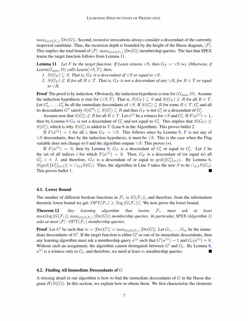
GetImmDe(G,G′′)

1. S ← S(G′′).2. While ∃f ∈ S(G) \ S such that

(∨S) ∨ f 6= G:3. S ← S ∪ {f}.4. Output(S).

GetAllImmDe(G)

1. De = {GetImmDe(G, 0)}.2. While G 6=

∨G′∈De

∧(S(G)\S(G′)):

3. Let a be a counterexample.4. De = De ∪ {GetImmDe(∨Z(G, a))}.5. Output(De).

Figure 2: Left: the GetImmDe operation. Right: the GetAllImmDe operation.

in H(S(G)) (compared to the other elements in F∨), which is necessary because the immediatedescendants are part of H(S(G)). We then give a characterization of the immediate descendants(compared to other descendants), which leads to an operation that computes an immediate descen-dant from a descendant. We finally show how to compute descendants that lead to obtaining diffe-rent immediate descendants. This completes the description of how SPEX can obtain all immediatedescendants.

By the definition of a representative, for every F ∈ F∨, GF = ∨f⇒F f. To decide whetherF ∈ F∨ is a representative, i.e., whether F ∈ G(F∨), we use Lemma 13 (whose proof directlyfollows from the definition of G(F∨)).

Lemma 13 Let F ∈ F∨. F ∈ G(F∨) if and only if for every f ∈ F\S(F ) we have F ∨ f 6= F .

Lemma 14 shows how to decide whether G′ is an immediate descendant of G.

Lemma 14 Let G,G′ ∈ G(F∨). G′ is an immediate descendant of G if and only if G′ 6= G,S(G′) ⊂ S(G) and for every f ∈ S(G)\S(G′) we have G′ ∨ f = G.

If G′ 6= G, S(G′) ⊂ S(G) and for some f ∈ S(G)\S(G′) we have G′ ∨ f 6= G, then GG′∨f isa descendant of G and an ascendant of G′.

Proof Only if: Let G′ be an immediate descendant of G, i.e., G′ 6= G, G′⇒G and S(G′) ⊂ S(G).Let f ∈ S(G)\S(G′). Since G′⇒(G′ ∨ f)⇒G and G′ 6= G′ ∨ f , we get G′ ∨ f = G.

If: Suppose G′ 6= G, G′⇒G and for every f ∈ S(G)\S(G′), we have G′ ∨ f = G. If G′ is notan immediate descendant of G, then let G′′ be a descendant of G and an immediate ascendant ofG′′. Take any f ∈ S(G′′)\S(G′) ⊂ S(G)\S(G′). Then, G′ ∨ f = G′′ 6= G – a contradiction. Thisalso proves the last statement of Lemma 14.

Lemma 14 shows how to compute an immediate descendant from a descendant, which we phrasein an operation called GetImmDe (Figure 2, left). GetImmDe takes G and a descendant G′′ of G(which can even be the zero function), initializes S = S(G′′), and as long as possible, repeatedlyextends S as follows: for f ∈ S(G)\S if (∨S) ∨ f 6= G, f is added to S.

GetImmDe can be used to obtain the first immediate descendant by calling it with G′′ = 0.We next show how to obtain a descendant for which GetImmDe will return a different immediatedescendant. To this end, we define the following: For G ∈ G(F∨) and a set X ′ ⊆ X , Z(G,X ′) ={f ∈ S(G) | f(X ′) = 0}, where f(X ′) = ∨x∈X′f(x). When X ′ = {x}, we abbreviate to Z(G, x).Obviously,

Z(G,X ′) =⋂

x∈X′Z(G, x). (1)

8


Lemma 15 relates this new definition to the descendants of G.

Lemma 15 Let G ∈ G(F∨) and X ′ ⊆ G−1(1) be a nonempty set. Then, G′ = ∨Z(G,X ′) ∈G(F∨) and G′ is a descendant of G.

For every immediate descendant G′ of G, there is X ′ ⊆ G−1(1) such that ∨Z(G,X ′) = G′.

Proof First notice that G′(X ′) = 0. Suppose on the contrary that G′ 6∈ G(F∨). Then, there isf ∈ S(G)\Z(G,X ′) such that G′ ∨ f = G′. Since f 6∈ Z(G,X ′), there is z ∈ X ′ such thatf(z) = 1 and then G′(X ′) = (G′ ∨ f)(X ′) 6= 0 – a contradiction. Therefore, G′ ∈ G(F∨). By thedefinition of Z, S(G′) ⊆ S(G) and thus G′ is a descendant of G.

Let G′ be an immediate descendant of G and let X ′ = {x ∈ X | G′(x) = 0 and G(x) = 1}.Then, X ′ ⊆ G−1(1). We now show Z(G,X ′) = S(G′). S(G′) ⊆ Z(G,X ′) because if f ∈ S(G′),then for all x ∈ X ′, f(x) = 0 and thus f ∈ Z(G,X ′). We next prove that Z(G,X ′) ⊆ S(G′).Let f ∈ Z(G,X ′) and x0 be a witness for G and G′, i.e., G(x0) = 1 and G′(x0) = 0. Therefore,x0 ∈ X ′ and f(x0) = 0 by the definition of Z. By Lemma 7, for every f ∈ S(G)\S(G′), we havef(a) = 1. Since f ∈ S(G), it must be that f ∈ S(G′).

Lemma 15 shows how to construct descendants from elements in X . Lemma 16 determineswhen all immediate descendants of G were obtained, and if not, how to obtain a new element inX that leads to a new immediate descendant. The algorithm that finds all immediate descendants(Figure 2, right) follows directly from this lemma. In the following we denote

∧S =

∧f∈S f .

Lemma 16 Let G1, . . . , Gm be immediate descendants of G. There is no other immediate descen-dant for G if and only if

G =m∨i=1

∧(S(G)\S(Gi)). (2)

If (2) does not hold, then for any counterexample a for (2), we have ∨Z(G, a) is a descendant of Gbut not equal to and not a descendant of any Gi, i = 1, . . . ,m.

Proof Only if: Suppose G 6= ∨mi=1 ∧ (S(G)\S(Gi)) and let a be a counterexample. Since for all i,S(G)\S(Gi) ⊆ S(G), we have ∨mi=1 ∧ (S(G)\S(Gi))⇒G. Therefore, G(a) = 1 and for every ithere is fi ∈ S(G)\S(Gi) such that fi(a) = 0. Consider G′ = Z(G, a). Since fi(a) = 0, we havefi ∈ S(G′). Since fi 6∈ S(Gi), G′ is not a descendant of Gi. Since G′ is a descendant of G and nota descendant of any Gi, there must be another immediate descendant of G.

If: Denote W =∨m

i=1

∧(S(G)\S(Gi)). Let G′ be another immediate descendant of G. Let

a be a witness for G and G′. Then G(a) = 1 and, by Lemma 7, for every f ∈ S(G)\S(G′),we have f(a) = 1 and for every f ∈ S(G′), we have f(a) = 0. Since S(G′) 6⊂ S(Gi), wehave S(G)\S(Gi) 6⊂ S(G)\S(G′), and therefore, (S(G)\S(Gi)) ∩ S(G′) is not empty. Choosefi ∈ (S(G)\S(Gi))∩S(G′). Then, fi ∈ S(G)\S(Gi) and since fi ∈ S(G′), fi(a) = 0. Therefore,W (a) = 0. Since G(a) = 1, we get G 6= W .

4.3. Critical Points

In this section, we show that if one can find certain points (the critical points), then the immediatedescendants can be computed in polynomial time (in the number of these points) and thus SPEX runs

9


in polynomial time. In particular, if the number of points is polynomial and they can be obtained inpolynomial time, then SPEX runs in polynomial time.

A set of points C ⊆ X is called a critical point set for F if for every S ⊆ F and if H =∧f∈S f ∧

∧f∈F\S f 6= 0, then there is a point in c ∈ C such that H(c) = 1.

We now show how to use the critical points to find the immediate descendants.

Lemma 17 Let C ⊆ X be a set of points. If C is a set of critical points for F , then all theimmediate descendants of G ∈ G(F∨) can be found in time |C| · |S(G)|.

Proof Let G1, . . . , Gm be some of the immediate descendants of G. To find another immediatedescendant we look for a point a such that G(a) = 1, and for every i, there is fi ∈ S(G)\S(Gi)such that fi(a) = 0. Let a be such point. Consider S = {f ∈ F | f(a) = 1} and letH =

∧f∈S f ∧

∧f∈F\S f . Since H(a) 6= 0, there is a critical point b ∈ C such that H(b) = 1.

By the definition of b, G(b) = 1 and for every i there is fi ∈ S(G)\S(Gi) such that fi(b) = 0.Therefore, b can be used to find a new descendant of G. To find the descendants we need, in theworst case, to substitute all the assignments of C in all the descendants G1, . . . , Gm and G. For allthe descendants, this takes at most |C| · |S(G)| steps, which implies the time complexity.

We now show how to generate the set of critical points.

Lemma 18 If for every S,R ⊆ F one can decide whether HS,R =∧

f∈S f ∧∧

f∈R f 6= 0 in timeT and if so, find a ∈ X such that HR,S(a) = 1, then a set of critical points C can be found in time|C| · T · |F|.

Proof The set is constructed inductively, in stages. Let F = {f1, . . . , ft} and denoteFi = {f1, . . . , fi}. Suppose we have a set Ki = {S ⊆ [i] |

∧f∈S f ∧

∧f∈[i]\S f 6= 0}; then we

define Ki+1 = {g ∧ fi+1 | g ∈ Ki and g ∧ fi+1 6= 0} ∪{g ∧ fi+1 | g ∈ Ki and g ∧ fi+1 6= 0}.

5. A Polynomial Time Algorithm for Halfspaces in a Constant Dimension

In this section, we show two results. The first is that when F is a set of halfspaces over a constantdimension, one can find a polynomial-sized critical point set in polynomial time, and therefore,SPEX can run in polynomial time. We then show that unless P = NP , this result cannot beextended to non-constant dimensions.

A halfspace of dimension d is a boolean function of the form:

f(x1, . . . , xd) = [a1x1 + · · ·+ adxd ≥ b] =

{1 if a1x1 + · · ·+ adxd ≥ b0 otherwise

where (x1, . . . , xd) ∈ <d and a1, . . . , ad, b are real numbers. Therefore, f : <d → {0, 1}.We now prove that the set of critical points is of a polynomial size.

Lemma 19 Let F be a set of halfspaces in dimension d. There is a set of critical points C for F ofsize |F|d+1.

10


Proof Define the dual set of halfspaces. That is, for every x ∈ <d, the dual functionx⊥ : F → {0, 1} where x⊥(f) = f(x). It is well known that the VC-dimension of this set is atmost d + 1. By the Sauer-Shelah lemma, the result follows.

Next, we prove that the set of critical points can be computed in polynomial time.

Lemma 20 Let F be a set of halfspaces in dimension d. A set of critical points C for F of size|F|d+1 can be found in time poly(|F|d).

Proof Follows from Lemma 18 and the fact that linear programming (required to check whetherg ∧ fi 6= 0) takes polynomial time.

By the above results, we conclude:

Theorem 21 Let F be a set of halfspaces in dimension d. There is a learning algorithm for F∨ thatruns in time |F|O(d) and asks at most |F| ·OPT(F∨) membership queries.

In particular, when the dimension d is constant, the algorithm runs in polynomial time.

Next, we show that the above cannot be extended to a non-constant dimension:

Theorem 22 If every set F of halfspaces deciding whether F ∈ F∨ is a descendant of ∨F can bedone in polynomial time, then P = NP .

Proof The reduction is from the problem of dual 3SAT – that is, given the literals{x1, . . . , xn, x1, . . . , xn} and the terms T1, . . . , Tm where each Ti is a conjunction of three liter-als, decide whether T1 ∨ · · · ∨ Tm = 1.

Given the terms T1, . . . , Tm, each can be translated into a halfspace. For example, the termx1 ∧ x2 ∧ x3 corresponds to the halfspace [x1 + (1− x2) + x3 ≥ 3] = [x1 − x2 + x3 ≥ 2]. Now,consider F = {T1, . . . , Tm, 1}. Then Gmax = 1 and T1 ∨ . . .∨Tm 6= 1 if and only if T1 ∨ · · · ∨Tm

is the only immediate descendant of Gmax.

6. Duality and a Polynomial Time Algorithm for Variable Inequality Predicates

In this section, we study the learnability of conjunctions over variable inequality predicates. Inthe acyclic case, we provide a polynomial time learning algorithm. In the general case, we showthat the learning problem is equivalent to the open problem of enumerating all the maximal acyclicsubgraphs of a given directed graph.

Consider the set of boolean functions FI := {[xi > xj ] |(i, j) ∈ I} for some I ⊆ [n]2 where[n] = {1, 2, . . . , n} and the variables xi are interpreted as real numbers. We define [xi > xj ] = 1 ifxi > xj ; and 0 otherwise. We assume throughout this section that (i, i) 6∈ I for all i.

We consider the dual class F∧ := {∧f∈Sf | S ⊆ F}. By duality (De Morgan’s law), all ourresults are true for learning F∧ (after swapping ∨ with ∧). The dual SPEX algorithm is depicted inFigure 3.

For a set J ⊆ I , we define FJ = ∧(i,j)∈J [xi > xj ]. For F ∈ FI∧ we define I(F ) = {(i, j) |

[xi > xj ] is in F}. Note that I(FJ) = J . For example, I([x1 > x2]∧ [x3 > x1]) = {(1, 2), (3, 1)}.

11


The directed graph of I ⊆ [n]2 is GI = ([n], I). The reachability matrix of I , denoted by R(I),is an n × n matrix where R(I)i,j = 1 if there is a (directed) path from i to j in GI ; otherwise,R(I)i,j = 0. We say that I is acyclic (resp., cyclic) if the graph GI is acyclic (resp., cyclic). Wesay that an assignment to the variables a ∈ [n]n is a topological sorting of I if for every (i, j) ∈ I ,we have ai > aj . It is known that I has a topological sorting if and only if I is acyclic. Also, it isknown that a topological sorting for an acyclic set can be found in linear time (see Knuth (1997),Volume 1, Section 2.2.3 and Cormen et al. (2001)). Next, we study the learnability of FI

∧ when I isacyclic and following this, we discuss the general case.

6.1. Acyclic Sets

We now examine the case when I is acyclic. Here, the number of critical points of FI whereI = {(1, 2), (2, 3), · · · , (n − 1, n)} is 2n−1. Therefore, using Lemma 17 does not enable us toobtain a polynomial time algorithm. Accordingly, we show a different way to determine whether afunction is a representative (i.e., in G(F∧)), and then show how to obtain the immediate descendantsin quadratic time (in n) and the witnesses in linear time. As a result, SPEX can run in polynomialtime. Finally, we show that the number of membership queries is at most |I|.

Before we show the main lemma, Lemma 24, we present Lemma 23, a trivial lemma that weuse to prove Lemma 24.

Lemma 23 Let I ⊆ [n]2 be an acyclic set, F ∈ FI∧, and a ∈ [n]n. Then, F (a) = 1 if and only if a

is a topological sorting of GI(F ).In particular, F is satisfiable and a satisfying assignment a ∈ [n]n can be found in linear time.

Next we show our main lemma that enables us to determine the representative elements and theimmediate descendants (in Lemmas 25–27). The proof is provided in Appendix C.

Lemma 24 Let I be acyclic and F1, F2 ∈ FI∧. Then, F1 = F2 if and only if R(I(F2))=R(I(F1)).

We now show how to decide whether F ∈ G(FI∧) – that is, whether F is a representative.

Lemma 25 Let I be an acyclic set and F ∈ FI∧. F ∈ G(FI

∧) if and only if for every (i, j) ∈I\I(F ) there is no path from i to j in GI(F ).

Proof If: If for every (i, j) ∈ I\I(F ) there is no path from i to j in GI(F ), then for every (i, j) ∈I\I(F ), R(I(F )∪ {(i, j)}) 6= R(I(F )) . By Lemma 24, this implies that F ∧ [xi > xj ] 6= F . By(the dual result of) Lemma 13, the result follows.

Only if: Now let F ∈ G(FI∧). By Lemma 13, for every [xi > xj ] 6∈ F , we have

F ∧ [xi > xj ] 6= F . Therefore, there is an assignment a that satisfies ai ≤ aj and F (a) = 1. Asbefore, if there is a path in GI(F ) from i to j, then we get a contradiction.

We now show how to determine the immediate descendants of G in polynomial time.

Lemma 26 Let I be acyclic. The immediate descendants of G ∈ G(FI∧) are all Gr,s :=

FI(G)\{(r,s)} where (r, s) ∈ I(G) and there is no path from r to s in GI(G)\{(r,s)}.In particular, for all G ∈ G(FI

∧), we have |De(G)| ≤ |I(G)| ≤ |I|.

The proof is in Appendix C. We now show how to find a witness.

12


Lemma 27 Let I be acyclic, G ∈ G(FI∧), and Gr,s := FI(G)\{(r,s)} be an immediate descendant

of G. A witness for G and Gr,s can be found in linear time.

Proof By Lemma 26, (r, s) ∈ I(G) and there is no path from r to s in GI(G)\{(r,s)}. Therefore, ifwe match vertices r and s in GI(G)\{(r,s)} we get an acyclic graph G′. Then, a topological sortinga for G′ is a satisfying assignment for Gr,s that satisfies ar = as. Since [xr > xs] ∈ S(G), we getG(a) = 0. Therefore, a is a witness for G and Gr,s.

To learn a function in FI∧, SPEX needs to find the immediate descendants of G and a witness for

each immediate descendant and G. By Lemma 26, this involves finding a path between every twonodes in the directed graph GI(G), which can be done in polynomial time. By Lemma 27, to find awitness, SPEX needs a topological sorting, which can be done in linear time. Therefore, SPEX runsin polynomial time. Therefore, by Theorem 10 and Lemma 26, the class FI

∧ is learnable in poly-nomial time with at most |I|2 membership queries. We now show that the number of membershipqueries is actually lower and equal to |I|.

Theorem 28 Let I ⊆ [n]2 be acyclic. The class FI∧ is learnable in polynomial time with at most

|I| membership queries.

Proof Consider the (dual) Algorithm SPEX in Figure 3 in Appendix A. Let F be the target function.Let Gmax = f1 ∧ f2 ∧ · · · ∧ ft where fi ∈ FI . By Lemma 26, we may assume w.l.o.g. thatG(i) = f1 ∧ f2 ∧ · · · ∧ fi−1 ∧ fi+1 ∧ · · · ft where i = 1, . . . , ` are all the immediate descendants ofG. Let a(i) be the witness for G and G(i), i = 1, . . . , `.

In the algorithm, S = {fi | i = 1, . . . , t}. If F (a(i)) = 1, then Line 5 in the algorithm removesfi from S and fi never returns to S. If F (a(i)) = 0, then the set {f1, f2, . . . , fi−1, fi+1, · · · ft}is added to T , which means (see Line 3) that SPEX never considers a descendant that does notcontain fi. Namely, for every fi, SPEX makes at most one membership query.

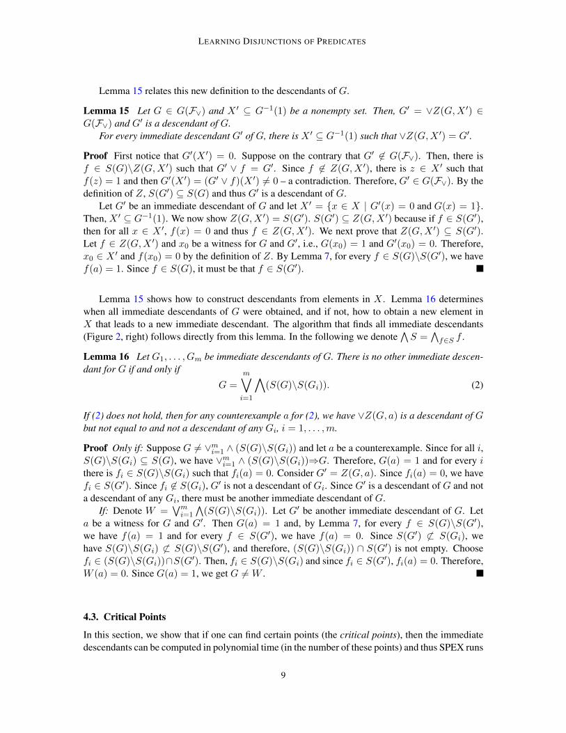
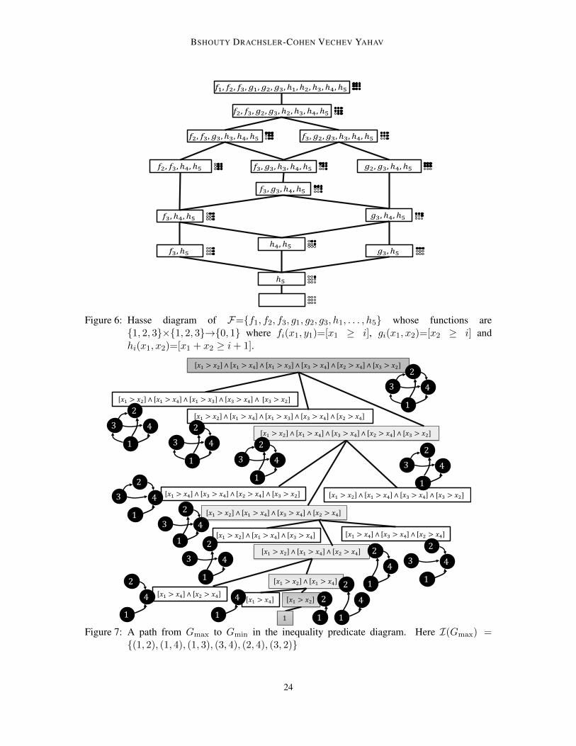
We conclude this section by illustrating SPEX on an example, depicted in Figure 7. Assume theset of boolean functions is FI , where I = {(1, 2), (1, 4), (1, 3), (3, 4), (2, 4), (3, 2)}, and the targetis Gmin = 1. The graph in Figure 7 shows the Hasse diagram (in white and gray nodes) and thecandidates that SPEX considers (in gray). The figure demonstrates that the number of membershipqueries is equal to |I|.

6.2. Cyclic Sets

In this section, we consider the general case, where I ⊆ [n]2 can be any set. Lemma 29 shows afew results when I is cyclic.

Lemma 29 Let I ⊆ [n]2 be any set with cycles. Then:1. Gmax = 0 is in FI

∧.2. The immediate descendants of Gmax are all ∧(i,j)∈J [xi > xj ] where GJ is a maximal acyclic

subgraph of GI .In particular,

3. Finding all the immediate descendants of Gmax is equivalent to enumerating all the maximalacyclic subgraphs of GI .

13


Proof If i1 → i2 → · · · → ic → i1 is a cycle, then Gmax⇒[xi1 > xi1 ] = 0 and thus Gmax = 0.If GJ is a maximal acyclic subgraph of GI , then adding any edge in I\J to GJ creates a cycle.

This implies that for any [xi > xj ] ∈ S(FI)\S(FJ), we have FJ ∧ [xi > xj ] = 0 = Gmax. ByLemma 14, FJ is an immediate descendant of Gmax.

Now, if FJ is an immediate descendant of Gmax, then J is acyclic because otherwiseFJ = 0 = Gmax. If GJ is not a maximal acyclic subgraph of GI , then there is an edge (i, j) suchthat J ∪{(i, j)} is acyclic and then either FJ∪{(i,j)} = FJ – in which case FJ is not a representativeand thus not an immediate descendant – or FJ∪{(i,j)} 6= FJ – in which case Gmax⇒FJ∪{(i,j)}⇒FJ

and Gmax 6= FJ∪{(i,j)} 6= FJ , and therefore, FJ is not an immediate descendant of Gmax.

Let G be any directed graph and denote by N(G) the number of the maximal acyclic subgraphsof G. Lemma 30 follows immediately from Theorem 12 and Lemma 29.

Lemma 30 OPT(FI∧) ≥ N(GI).

The problem of enumerating all the maximal acyclic subgraphs of a directed graph is still anopen problem (Acua et al., 2012; Borassi et al., 2013; Wasa, 2016). We show that learning a functionin FI

∧ (where I ⊆ [n]2) in polynomial time is possible if and only if the enumeration problem canbe done in polynomial time (the proof is in Appendix C).

Theorem 31 There is a polynomial time learning algorithm (poly(OPT(FI∧), n, |I|)), which for

an input I ⊆ [n]2, learns F ∈ FI∧ if and only if there is an algorithm that for an input G, which

is a directed graph, enumerates all the maximal acyclic subgraphs of G(V,E) in polynomial time(poly(N(G), |V |, |E|)).

7. Application to Program Synthesis

In this section, we explain the natural integration of SPEX into program synthesis. We then de-monstrate this on a synthesizer that synthesizes programs that detect patterns in time-series charts.These programs meet specifications that belong to the class of variable inequalities I (for acyclic I).

Program synthesizers are defined over an input domain Xin, an output domain Xout, and adomain-specific language D. Given a specification, the goal of a synthesizer is to generate a corre-sponding program. A specification is a set of formulas ϕ(xin, xout) where xin is interpreted overXin and xout is interpreted over Xout. Given a specification Y , a synthesizer returns a programP : Xin → Xout over D such that for all in ∈ Xin: (in, P (in)) |= Y (i.e., all formulas aresatisfied for xin = in and xout = out). Roughly speaking, there are two types of synthesizers:• Synthesizers that assume that Y describes a full specification. Namely, for all in ∈ Xin, there

exists a single out ∈ Xout such that (in, out) |= Y (e.g., Solar-Lezama et al. (2008); Singhand Solar-Lezama (2011); Alur et al. (2013); Bornholt et al. (2016)).• Synthesizers that assume that Y describes only input–output examples (known as PBE synt-

hesizers). Namely, all formulas in the specification take the form of xin = in⇒xout = out(e.g., Gulwani (2011); Polozov and Gulwani (2015); Barowy et al. (2015)). The typical set-ting of a PBE synthesizer is that an end user (that acts as the teacher) knows a target programf and he or she provides the synthesizer with some initial examples and can interact with thesynthesizer through membership queries (we note that most synthesizers do not interact).

14


Each approach has its advantages and disadvantages. The first approach guarantees correctnesson all inputs, but requires a full specification, which is complex to provide, especially by end usersunfamiliar with formulas. On the other hand, PBE synthesizers are user-friendly as they interactthrough examples; however, generally they do not guarantee correctness on all inputs.

We next define the class of programs that are F-describable. For such programs, SPEX canbe leveraged by both approaches to eliminate their disadvantage. Let F be a set of predicates overXin ∪ Xout. A synthesizer is F-describable if every program that can be synthesized meets aspecification F ∈ F∨ (or dually, F∧). A synthesizer that assumes that Y is a full specification andis F-describable can release the user from having to provide the full specification by first runningSPEX and then synthesizing a program from the formula returned by SPEX. A PBE synthesizer thatis F-describable can be extended to guarantee correctness on all inputs by first running SPEX andthen synthesizing the program from the set of membership queries posed by SPEX. Theorem 32follows immediately from Theorem 10.

Theorem 32 LetF be a set of predicates andA be anF-describable synthesizer. Then,A extendedwith SPEX returns the target program with at most |F| ·maxG∈G(F∨) |De(G)| membership queries.

7.1. Example: Synthesis of Time-series Patterns

In this section, we consider the setting of synthesizing programs that detect time-series patterns.The specifications of these programs are over FI

∧ for some I ⊆ [n]2 and thus the synthesizer learnsthe target program within |I| membership queries. Time-series are used in many domains includingfinancial analysis (Bulkowski, 2005), medicine (Chuah and Fu, 2007), and seismology (Morales-Esteban et al., 2010). Experts use these charts to predict important events (e.g., trend changes instock prices) by looking for patterns in the charts. There are a variety of platforms that enable usersto write programs to detect a pattern in a time-series chart. In this work, we consider a domain-specific language (DSL) of a popular trading platform, AmiBroker. Our synthesizer can easily beextended to other DSLs.

A time-series chart c : N → R maps points in time to real values (e.g., stock prices). A time-series pattern is a conjunction FI for acyclic I . The size of FI is the maximal natural number itcontains, i.e., the size of FI is argmaxi{i | ∃j.(i, j) ∈ I or (j, i) ∈ I}. A program detects a patternFI of size k in a time-series chart c if it alerts upon every t ∈ N for which the t1, ..., tk−1 precedingextreme points satisfy FI(c(t1), ..., c(tk−1), c(t)) = 1.

In this setting, Xin is a set of charts over a fixed k ∈ N, that is f : {1, ..., k} → R, andXout = {0, 1}. The DSL D is the DSL of the trading platform AmiBroker. We built a synthesizerthat not only interacts with the end user through membership queries, but also displays them ascharts (of size k). Thereby, our synthesizer communicates with the end user in his language ofexpertise. The synthesizer takes as input an initial chart example c′ : {1, ..., k} → R and initializesI to {(i, j) ∈ [k]2 | c′(i) ≥ c′(j)} and sets FI := {[xi ≥ xj ] |(i, j) ∈ I} (our results are truealso for these kinds of predicates). It then executes SPEX to learn F . During the execution, everywitness is translated into a chart (the translation is immediate since each witness is an assignmentto k points). Finally, our synthesizer synthesizes a program by synthesizing instructions that detectthe k extreme points in the chart, followed by an instruction that checks whether these points satisfythe formula F and alerts the end user if so (the technical details are beyond the scope of this paper).Namely, for the end user, our synthesizer acts as a PBE synthesizer, but internally it takes the firstsynthesis approach and assumes it is given a full specification (which is obtained by running SPEX).

15


The complexity of the overall synthesis algorithm is determined by SPEX (as the synthesis merelysynthesizes the instructions according to the specification F ), and thus from Theorem 28, we inferthe following theorem.

Theorem 33 The pattern synthesizer returns a program that detects the target pattern in polynomialtime with at most k2 membership queries, where k is the target pattern size.

8. Related Work

Program Synthesis Program synthesis has drawn a lot of attention over the last decade, especiallyin the setting of synthesis from examples, known as PBE (e.g., Gulwani (2010); Lau et al. (2003);Das Sarma et al. (2010); Harris and Gulwani (2011); Gulwani (2011); Gulwani et al. (2012); Singhand Gulwani (2012); Yessenov et al. (2013); Albarghouthi et al. (2013); Zhang and Sun (2013);Menon et al. (2013); Le and Gulwani (2014); Barowy et al. (2015); Polozov and Gulwani (2015)).Commonly, PBE algorithms synthesize programs consistent with the examples, which may not cap-ture the user intent. Some works, however, guarantee to output the target program. For example,CEGIS (Solar-Lezama, 2008) learns a program via equivalence queries, and oracle-based synthe-sis (Jha et al., 2010) assumes that the input space is finite, which allows it to guarantee correctnessby exploring all inputs (i.e., without validation queries). Synthesis has also been studied in a settingwhere a specification and the program’s syntax are given and the goal is to find a program over thissyntax meeting the specification (e.g., Solar-Lezama et al. (2008); Singh and Solar-Lezama (2011);Alur et al. (2013); Bornholt et al. (2016)).

Queries over Streams Several works aim to help analysts. Many trading software platforms pro-vide domain-specific languages for writing queries where the user defines the query and the systemis responsible for the sliding window mechanism, e.g., MetaTrader, MetaStock, NinjaTrader, andMicrosoft’s StreamInsight (Chandramouli et al., 2010). Another tool designed to help analysts isStat! (Barnett et al., 2013), an interactive tool enabling analysts to write queries in StreamInsight.TimeFork (Badam et al., 2016) is an interactive tool that helps analysts with predictions based onautomatic analysis of the past stock price. CPL (Anand et al., 2001) is a Haskell-based high-levellanguage designed for chart pattern queries. Many other languages support queries for streams.SASE (Wu et al., 2006) is a system designed for RFID (radio frequency identification) streams thatoffers a user-friendly language and can handle large volumes of data. Cayuga (Brenna et al., 2007)is a system for detecting complex patterns in streams, whose language is based on Cayuga algebra.SPL (Hirzel et al., 2013) is IBM’s stream processing language supporting pattern detections. Acti-veSheets (Vaziri et al., 2014) is a platform that enables Microsoft Excel to process real-time streamsfrom within spreadsheets.

9. Conclusion

In this paper, we have studied the learnability of disjunctions F∨ (and conjunctions) over a setof boolean functions F . We have shown an algorithm SPEX that asks at most |F| · OPT (F∨)membership queries. We further showed two classes that SPEX can learn in polynomial time.We then showed a practical application of SPEX that augments PBE synthesizers, giving them theability to guarantee to output the target program as the end user intended. Lastly, we showed a

16

www.metaquotes.net

www.metastock.com

www.ninjatrader.com


synthesizer that learns time-series patterns in polynomial time and outputs an executable program,while interacting with the end user through visual charts.

Acknowledgements The research leading to these results has received funding from the EuropeanUnion’s - Seventh Framework Programme (FP7) under grant agreement no 615688–ERC-COG-PRIME.

References

Hasan Abasi, Ali Z. Abdi, and Nader H. Bshouty. Learning boolean halfspaces with small weightsfrom membership queries. In Algorithmic Learning Theory: 25th International Conference, ALT’14, 2014.

Elias Abboud, Nader Agha, Nader H. Bshouty, Nizar Radwan, and Fathi Saleh. Learning thresholdfunctions with small weights using membership queries. In Proceedings of the Twelfth AnnualConference on Computational Learning Theory, COLT ’99, pages 318–322, 1999.

Vicente Acua, Etienne Birmel, Ludovic Cottret, Pierluigi Crescenzi, Fabien Jourdan, Vincent La-croix, Alberto Marchetti-Spaccamela, Andrea Marino, Paulo Vieira Milreu, Marie-France Sagot,and Leen Stougie. Telling stories: Enumerating maximal directed acyclic graphs with a constrai-ned set of sources and targets. Theoretical Computer Science, 457:1 – 9, 2012.

Aws Albarghouthi, Sumit Gulwani, and Zachary Kincaid. Recursive program synthesis. In Compu-ter Aided Verification - 25th International Conference, CAV ’13, pages 934–950, 2013.

Noga Alon, Richard Beigel, Simon Kasif, Steven Rudich, and Benny Sudakov. Learning a hiddenmatching. In Proceedings of the 43rd Symposium on Foundations of Computer Science, FOCS’02, 2002.

Rajeev Alur, Rastislav Bodik, Garvit Juniwal, Milo M. K. Martin, Mukund Raghothaman, Sanjit A.Seshia, Rishabh Singh, Armando Solar-Lezama, Emina Torlak, and Abhishek Udupa. Syntax-guided synthesis. In Formal Methods in Computer-Aided Design, FMCAD ’13, pages 1–8, 2013.

AmiBroker. https://www.amibroker.com/.

Saswat Anand, Wei-Ngan Chin, and Siau-Cheng Khoo. Charting patterns on price history. InProceedings of the Sixth ACM SIGPLAN International Conference on Functional Programming(ICFP ’01), pages 134–145, 2001.

Dana Angluin. Queries and concept learning. Machine Learning, 2(4):319–342, 1988.

Dana Angluin and Jiang Chen. Learning a hidden graph using queries per edge. Journal of Com-puter and System Sciences, 74(4):546 – 556, 2008. Carl Smith Memorial Issue.

Sriram Karthik Badam, Jieqiong Zhao, Shivalik Sen, Niklas Elmqvist, and David S. Ebert. Time-fork: Interactive prediction of time series. In Proceedings of the 2016 CHI Conference on HumanFactors in Computing Systems, pages 5409–5420, 2016.

17

https://www.amibroker.com/


Mike Barnett, Badrish Chandramouli, Robert DeLine, Steven Drucker, Danyel Fisher, JonathanGoldstein, Patrick Morrison, and John Platt. Stat!: An interactive analytics environment for bigdata. In Proceedings of the ACM SIGMOD International Conference on Management of Data,SIGMOD ’13, pages 1013–1016, 2013.

Daniel W. Barowy, Sumit Gulwani, Ted Hart, and Benjamin Zorn. Flashrelate: Extracting relati-onal data from semi-structured spreadsheets using examples. In Proceedings of the 36th ACMSIGPLAN Conference on Programming Language Design and Implementation, PLDI ’15, pages218–228, 2015.

E. Biglieri and L. Gyrfi. Multiple Access Channels: Theory and Practice. IOS Press, 2007.

Annalisa De Bonis, Leszek Gasieniec, and Ugo Vaccaro. Optimal two-stage algorithms for grouptesting problems. volume 34, pages 1253–1270, 2005.

Michele Borassi, Pierluigi Crescenzi, Vincent Lacroix, Andrea Marino, Marie-France Sagot, andPaulo Vieira Milreu. Telling stories fast. In Vincenzo Bonifaci, Camil Demetrescu, and AlbertoMarchetti-Spaccamela, editors, Experimental Algorithms: 12th International Symposium, SEA’13, pages 200–211, 2013.

James Bornholt, Emina Torlak, Dan Grossman, and Luis Ceze. Optimizing synthesis with metas-ketches. In Proceedings of the 43rd Annual ACM SIGPLAN-SIGACT Symposium on Principlesof Programming Languages, POPL ’16, pages 775–788, 2016.

Lars Brenna, Alan Demers, Johannes Gehrke, Mingsheng Hong, Joel Ossher, Biswanath Panda, Mi-rek Riedewald, Mohit Thatte, and Walker White. Cayuga: A high-performance event processingengine. In Proceedings of the ACM SIGMOD International Conference on Management of Data,pages 1100–1102, 2007.

Thomas N. Bulkowski. Encyclopedia of Chart Patterns. Wiley, 2nd edition, 2005.

Badrish Chandramouli, Jonathan Goldstein, and David Maier. High-performance dynamic patternmatching over disordered streams. In PVLDB, volume 3, pages 220–231, 2010.

Mooi Choo Chuah and Fen Fu. Ecg anomaly detection via time series analysis. In Frontiers ofHigh Performance Computing and Networking ISPA 2007 Workshops: ISPA 2007 InternationalWorkshops SSDSN, UPWN, WISH, SGC, ParDMCom, HiPCoMB, and IST-AWSN, pages 123–135, 2007.

Ferdinando Cicalese. Group testing. In Fault-Tolerant Search Algorithms, pages 139–173. Springer,2013.

Thomas H. Cormen, Clifford Stein, Ronald L. Rivest, and Charles E. Leiserson. Introduction toAlgorithms. McGraw-Hill Higher Education, 2nd edition, 2001.

Anish Das Sarma, Aditya Parameswaran, Hector Garcia-Molina, and Jennifer Widom. Synthesizingview definitions from data. In Database Theory - ICDT ’10, 13th International Conference, pages89–103, 2010.

18


Robert Dorfman. The detection of defective members of large populations. The Annals of Mathe-matical Statistics, 14(4):436–440, 1943.

D. Du and F. Hwang. Combinatorial Group Testing and Its Applications. Applied Mathematics.World Scientific, 2000.

D. Du and F. Hwang. Pooling Designs and Nonadaptive Group Testing: Important Tools for DNASequencing. Series on applied mathematics. World Scientific, 2006.

Vladimir Grebinski and Gregory Kucherov. Reconstructing a hamiltonian cycle by querying thegraph: Application to DNA physical mapping. Discrete Appl. Math., 88(1-3):147–165, Novem-ber 1998.

Sumit Gulwani. Dimensions in program synthesis. In Proceedings of the 12th International ACMSIGPLAN Conference on Principles and Practice of Declarative Programming, pages 13–24,2010.

Sumit Gulwani. Automating string processing in spreadsheets using input-output examples. In Pro-ceedings of the 38th ACM SIGPLAN-SIGACT Symposium on Principles of Programming Lan-guages, POPL ’11, pages 317–330, 2011.

Sumit Gulwani, William R. Harris, and Rishabh Singh. Spreadsheet data manipulation using exam-ples. Commun. ACM, 55(8):97–105, 2012.

William R. Harris and Sumit Gulwani. Spreadsheet table transformations from examples. In Pro-ceedings of the 32nd ACM SIGPLAN Conference on Programming Language Design and Imple-mentation, PLDI ’11, pages 317–328, 2011.

Tibor Hegedus. Generalized teaching dimensions and the query complexity of learning. In Pro-ceedings of the Eighth Annual Conference on Computational Learning Theory, COLT ’95, pages108–117, 1995.

M. Hirzel, H. Andrade, B. Gedik, G. Jacques-Silva, R. Khandekar, V. Kumar, M. Mendell, H. Nas-gaard, S. Schneider, R. Soule, and K.-L. Wu. IBM streams processing language: Analyzing bigdata in motion. IBM J. Res. Dev., 57(3-4), 2013.

Susmit Jha, Sumit Gulwani, Sanjit A. Seshia, and Ashish Tiwari. Oracle-guided component-basedprogram synthesis. In Proceedings of the 32nd ACM/IEEE International Conference on SoftwareEngineering - Volume 1, ICSE ’10, pages 215–224, 2010.

Donald E. Knuth. The Art of Computer Programming, Volume 1 (3rd Ed.): Fundamental Algo-rithms. Addison Wesley Longman Publishing Co., Inc., Redwood City, CA, USA, 1997.

Tessa A. Lau, Steven A. Wolfman, Pedro Domingos, and Daniel S. Weld. Programming by demon-stration using version space algebra. Machine Learning, 53(1-2):111–156, 2003.

Vu Le and Sumit Gulwani. Flashextract: A framework for data extraction by examples. In ACMSIGPLAN Conference on Programming Language Design and Implementation, PLDI ’14, pages542–553, 2014.

19


Aditya Krishna Menon, Omer Tamuz, Sumit Gulwani, Butler W. Lampson, and Adam Kalai. A ma-chine learning framework for programming by example. In Proceedings of the 30th InternationalConference on Machine Learning, ICML ’13, pages 187–195, 2013.

A. Morales-Esteban, F. Martnez-lvarez, A. Troncoso, J.L. Justo, and C. Rubio-Escudero. Patternrecognition to forecast seismic time series. Expert Systems with Applications, 37(12):8333 –8342, 2010.

Hung Q Ngo and Ding-Zhu Du. A survey on combinatorial group testing algorithms with ap-plications to DNA library screening. DIMACS Series in Discrete Mathematics and TheoreticalComputer Science, 2000.

Andrzej Pelc. Searching games with errors—fifty years of coping with liars. Theor. Comput. Sci.,270(1-2):71–109, January 2002.

Oleksandr Polozov and Sumit Gulwani. Flashmeta: A framework for inductive program synthe-sis. In Proceedings of the 2015 ACM SIGPLAN International Conference on Object-OrientedProgramming, Systems, Languages, and Applications, OOPSLA ’15, pages 107–126, 2015.

Rishabh Singh and Sumit Gulwani. Learning semantic string transformations from examples.PVLDB, 5(8):740–751, 2012.

Rishabh Singh and Armando Solar-Lezama. Synthesizing data structure manipulations from story-boards. In SIGSOFT/FSE’11 19th ACM SIGSOFT Symposium on the Foundations of SoftwareEngineering (FSE-19) and ESEC’11: 13th European Software Engineering Conference (ESEC-13), pages 289–299, 2011.

Armando Solar-Lezama. Program synthesis by sketching. ProQuest, 2008.

Armando Solar-Lezama, Christopher Grant Jones, and Rastislav Bodik. Sketching concurrent datastructures. In Proceedings of the ACM SIGPLAN 2008 Conference on Programming LanguageDesign and Implementation, pages 136–148, 2008.

Mandana Vaziri, Olivier Tardieu, Rodric Rabbah, Philippe Suter, and Martin Hirzel. Stream pro-cessing with a spreadsheet. In ECOOP 2014 - Object-Oriented Programming - 28th EuropeanConference, pages 360–384. 2014.

Kunihiro Wasa. Enumeration of enumeration algorithms. CoRR, abs/1605.05102, 2016.

Eugene Wu, Yanlei Diao, and Shariq Rizvi. High-performance complex event processing overstreams. In Proceedings of the ACM SIGMOD International Conference on Management ofData, pages 407–418, 2006.

Kuat Yessenov, Shubham Tulsiani, Aditya Krishna Menon, Robert C. Miller, Sumit Gulwani, But-ler W. Lampson, and Adam Kalai. A colorful approach to text processing by example. In The 26thAnnual ACM Symposium on User Interface Software and Technology, UIST’13, pages 495–504,2013.

Sai Zhang and Yuyin Sun. Automatically synthesizing sql queries from input-output examples. In2013 28th IEEE/ACM International Conference on Automated Software Engineering, ASE ’13,pages 224–234, 2013.

20


N. Yu. Zolotykh and V. N. Shevchenko. Deciphering threshold functions of k-valued logic. InDiscrete Analysis and Operations Research. Novosibirsk 2(3), pp. 18. English translation: Kors-hunov, A. D. (ed.): Operations Research and Discrete Analysis. Kluwer Ac. Publ. Netherlands.(1997), 1995.

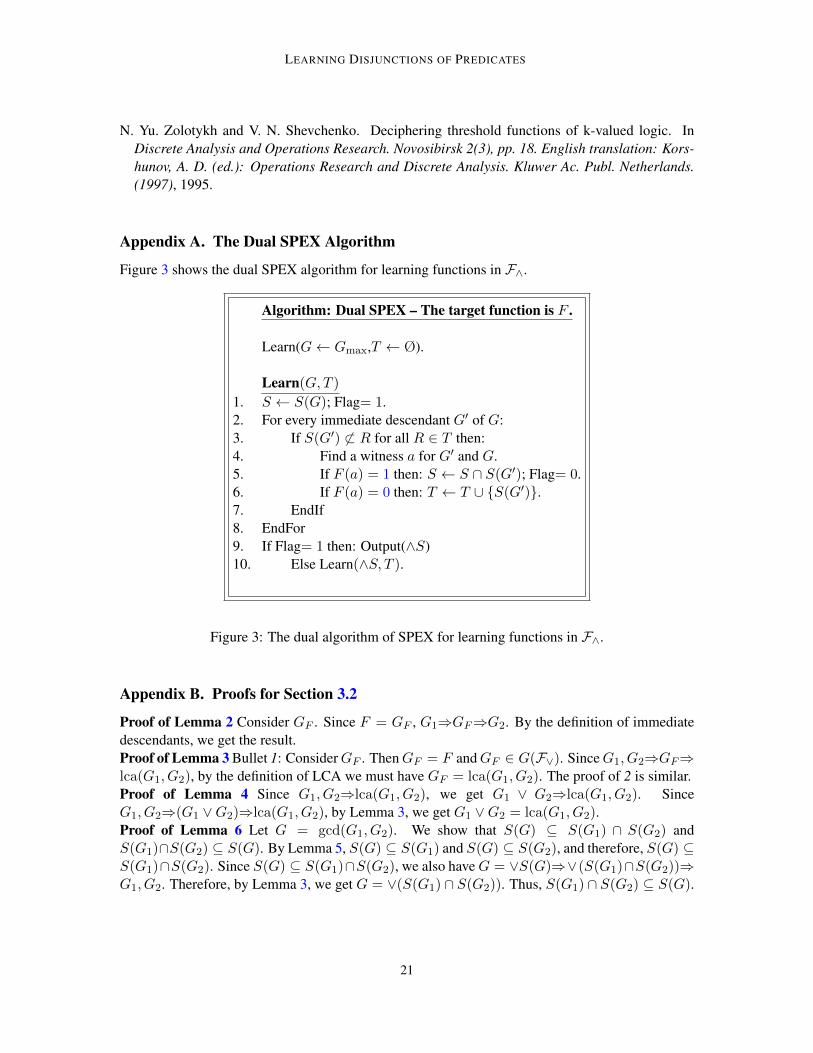
Appendix A. The Dual SPEX Algorithm

Figure 3 shows the dual SPEX algorithm for learning functions in F∧.

Algorithm: Dual SPEX – The target function is F .

Learn(G← Gmax,T ← Ø).

Learn(G,T )

1. S ← S(G); Flag= 1.2. For every immediate descendant G′ of G:3. If S(G′) 6⊂ R for all R ∈ T then:4. Find a witness a for G′ and G.5. If F (a) = 1 then: S ← S ∩ S(G′); Flag= 0.6. If F (a) = 0 then: T ← T ∪ {S(G′)}.7. EndIf8. EndFor9. If Flag= 1 then: Output(∧S)10. Else Learn(∧S, T ).

Figure 3: The dual algorithm of SPEX for learning functions in F∧.

Appendix B. Proofs for Section 3.2

Proof of Lemma 2 Consider GF . Since F = GF , G1⇒GF⇒G2. By the definition of immediatedescendants, we get the result.Proof of Lemma 3 Bullet 1: Consider GF . Then GF = F and GF ∈ G(F∨). Since G1, G2⇒GF⇒lca(G1, G2), by the definition of LCA we must have GF = lca(G1, G2). The proof of 2 is similar.Proof of Lemma 4 Since G1, G2⇒lca(G1, G2), we get G1 ∨ G2⇒lca(G1, G2). SinceG1, G2⇒(G1 ∨G2)⇒lca(G1, G2), by Lemma 3, we get G1 ∨G2 = lca(G1, G2).Proof of Lemma 6 Let G = gcd(G1, G2). We show that S(G) ⊆ S(G1) ∩ S(G2) andS(G1)∩S(G2) ⊆ S(G). By Lemma 5, S(G) ⊆ S(G1) and S(G) ⊆ S(G2), and therefore, S(G) ⊆S(G1)∩S(G2). Since S(G) ⊆ S(G1)∩S(G2), we also have G = ∨S(G)⇒∨(S(G1)∩S(G2))⇒G1, G2. Therefore, by Lemma 3, we get G = ∨(S(G1) ∩ S(G2)). Thus, S(G1) ∩ S(G2) ⊆ S(G).

21


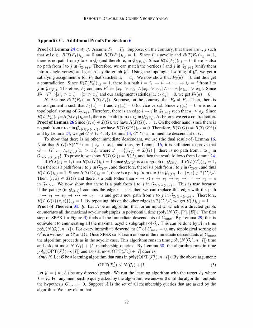
Appendix C. Additional Proofs for Section 6

Proof of Lemma 24 Only if: Assume F1 = F2. Suppose, on the contrary, that there are i, j suchthat w.l.o.g. R(I(F1))i,j = 0 and R(I(F2))i,j = 1. Since I is acyclic and R(I(F2))i,j = 1,there is no path from j to i in GI (and therefore, in GI(F1)). Since R(I(F1))i,j = 0, there is alsono path from i to j in GI(F1). Therefore, we can match the vertices i and j in GI(F1) (unify theminto a single vertex) and get an acyclic graph G′. Using the topological sorting of G′, we get asatisfying assignment a for F1 that satisfies ai = aj . We now show that F2(a) = 0 and thus geta contradiction. Since R(I(F2))i,j = 1, there is a path i = i1 → i2 → · · · → i` = j from i toj in GI(F2). Therefore, F2 contains F ′ := [xi1 > xi2 ] ∧ [xi2 > xi3 ] ∧ · · · ∧ [xi`−1

> xi` ]. SinceF2⇒F ′⇒[xi1 > xi` ] = [xi > xj ] and our assignment satisfies [ai > aj ] = 0, we get F2(a) = 0.

If: Assume R(I(F2)) = R(I(F1)). Suppose, on the contrary, that F2 6= F1. Then, there isan assignment a such that F2(a) = 1 and F1(a) = 0 (or vice versa). Since F1(a) = 0, a is not atopological sorting of GI(F1). Therefore, there is an edge i → j in GI(F1) such that ai ≤ aj . SinceR(I(F2))i,j=R(I(F1))i,j=1, there is a path from i to j in GI(F2). As before, we get a contradiction.Proof of Lemma 26 Since (r, s) ∈ I(G), we have R(I(G))r,s=1. On the other hand, since there isno path from r to s in GI(G)\{(r,s)}, we have R(I(Gr,s))r,s = 0. Therefore, R(I(G)) 6= R(I(Gr,s))and by Lemma 24, we get G 6= Gr,s. By Lemma 14, Gr,s is an immediate descendant of G.

To show that there is no other immediate descendant, we use (the dual result of) Lemma 16.Note that S(G)\S(Gr,s) = {[xr > xs]} and thus, by Lemma 16, it is sufficient to prove thatG = G′ := ∧(i,j)∈J [xi > xj ], where J = {(i, j) ∈ I(G) | there is no path from i to j inGI(G)\{(i,j)}}. To prove it, we show R(I(G′)) = R(J), and then the result follows from Lemma 24.

If R(J)i,j = 1, then R(I(G′))i,j = 1 since GI(G′) is a subgraph of GI(G). If R(I(G′))i,j = 1,then there is a path from i to j in GI(G′), and therefore, there is a path from i to j in GI(G), and thusR(I(G))i,j = 1. Since R(I(G))i,j = 1, there is a path p from i to j in GI(G). Let (r, s) 6∈ I(G)\J .Then, (r, s) ∈ I(G) and there is a path (other than r → s) r → v1 → v2 → · · · → v` = sin GI(G). We now show that there is a path from i to j in GI(G)\{(r,s)}. This is true becauseif the path p (in GI(G)) contains the edge r → s, then we can replace this edge with the pathr → v1 → v2 → · · · → v` = s and get a new path from i to j in GI(G)\{(r,s)}. Therefore,R(I(G)\{(r, s)})i,j = 1. By repeating this on the other edges in I(G)\J , we get R(J)i,j = 1.Proof of Theorem 31: If: Let A be an algorithm that for an input G, which is a directed graph,enumerates all the maximal acyclic subgraphs in polynomial time (poly(N(G), |V |, |E|)). The firststep of SPEX (in Figure 3) finds all the immediate descendants of Gmax. By Lemma 29, this isequivalent to enumerating all the maximal acyclic subgraphs of GI . This can be done by A in timepoly(N(GI), n, |I|). For every immediate descendant G′ of Gmax = 0, any topological sorting ofG′ is a witness for G′ and G. Once SPEX calls Learn on one of the immediate descendants of Gmax,the algorithm proceeds as in the acyclic case. This algorithm runs in time poly(N(GI), n, |I|) timeand asks at most N(GI) + |I| membership queries. By Lemma 30, the algorithm runs in timepoly(OPT(FI

∧), n, |I|) and asks at most OPT(FI∧) + |I| queries.

Only if: Let B be a learning algorithm that runs in poly(OPT(FI∧), n, |I|). By the above argument:

OPT(FI∧) ≤ N(GI) + |I|. (3)

Let G = ([n], E) be any directed graph. We run the learning algorithm with the target FI whereI = E. For any membership query asked by the algorithm, we answer 0 until the algorithm outputsthe hypothesis Gmax = 0. Suppose A is the set of all membership queries that are asked by thealgorithm. We now claim that:

22


𝑓11 ∨ 𝑓12 ∨ 𝑓21 ∨ 𝑓22

𝑓12 ∨ 𝑓22

𝑓22𝑓12

0

{𝑓12, 𝑓22}

{𝑓22}

∅

{𝑓11, 𝑓12, 𝑓21, 𝑓22}

{𝑓12}

Figure 4: Left: the Hasse diagram of Ray22. Right: the corresponding S(G) sets.

𝑥1 ∨ 𝑥2 ∨ 𝑥3

0

𝑥1 ∨ 𝑥2 𝑥1 ∨ 𝑥3 𝑥2 ∨ 𝑥3

𝑥1 𝑥2 𝑥3

𝑥1 ∨ 𝑥2 ∨ 𝑥1 ∨ 𝑥2

0

𝑥1 ∨ 𝑥2 𝑥1 ∨ 𝑥2 𝑥2 ∨ 𝑥1

𝑥1 𝑥2 𝑥1

𝑥1 ∨ 𝑥2

𝑥2

Figure 5: Hasse diagram of terms and monotone terms.

1. |A| = poly(N(G), n, |E|).2. If G′ is a maximal acyclic subgraph of G, then there is an assignment a ∈ A such that

E(G′) = {(i, j) ∈ E | ai > aj}, where E(G′) is the set of edges of G′.Bullet 1 follows since B runs in time poly(OPT(FI

∧), n, |I|) and by (3) this is poly(N(G), n, |E|).So the number of membership queries cannot be more than poly(N(G), n, |E|) time.

We now prove bullet 2. There is an assignment a ∈ A that satisfies FE(G′)(a) = 1, because ot-herwise the algorithm cannot distinguish between FE(G′) and Gmax, which violates the correctnessof the algorithm. Now, since FE(G′)(a) = 1, we must have E(G′) ⊆ {(i, j) ∈ E | ai > aj}. SinceE(G′) is maximal (adding another edge will create a cycle), we get E(G′) = {(i, j) ∈ E | ai > aj}.

The algorithm that enumerates all the maximal acyclic subgraphs of G(V,E) continues to runas follows: for each a ∈ A, it defines Ea := {(i, j) ∈ E | ai > aj}. If Ga := ([n], Ea) is amaximal cyclic subgraph, then it lists Ga. Testing whether Ga := ([n], Ea) is maximal can be donein polynomial time (e.g., by checking edge-by-edge in E). It is easy to verify that the algorithmruns in poly(N(G), |V |, |E|) time.

Appendix D. Additional Figures

Here, we provide Figures 4, 5, 6, and 7.

23


𝑓1, 𝑓2, 𝑓3, 𝑔1, 𝑔2, 𝑔3, ℎ1, ℎ2, ℎ3, ℎ4, ℎ5

𝑓2, 𝑓3, 𝑔2, 𝑔3, ℎ2, ℎ3, ℎ4, ℎ5

𝑓2, 𝑓3, 𝑔3, ℎ3, ℎ4, ℎ5

𝑓2, 𝑓3, ℎ4, ℎ5

𝑓3, ℎ4, ℎ5

𝑓3, ℎ5

ℎ5

𝑓3, 𝑔2, 𝑔3, ℎ3, ℎ4, ℎ5

𝑔2, 𝑔3, ℎ4, ℎ5

𝑔3, ℎ4, ℎ5

𝑔3, ℎ5

𝑓3, 𝑔3, ℎ3, ℎ4, ℎ5

𝑓3, 𝑔3, ℎ4, ℎ5

ℎ4, ℎ5

Figure 6: Hasse diagram of F={f1, f2, f3, g1, g2, g3, h1, . . . , h5} whose functions are{1, 2, 3}×{1, 2, 3}→{0, 1} where fi(x1, y1)=[x1 ≥ i], gi(x1, x2)=[x2 ≥ i] andhi(x1, x2)=[x1 + x2 ≥ i + 1].

𝑥1 > 𝑥4 ∧ 𝑥3 > 𝑥4 ∧ 𝑥2 > 𝑥4

𝑥1 > 𝑥2 ∧ 𝑥1 > 𝑥4 ∧ 𝑥3 > 𝑥4 ∧ [𝑥3 > 𝑥2]

𝑥1 > 𝑥2 ∧ 𝑥1 > 𝑥4 ∧ 𝑥3 > 𝑥4

𝑥1 > 𝑥2 ∧ 𝑥1 > 𝑥4 ∧ 𝑥3 > 𝑥4 ∧ 𝑥2 > 𝑥4

𝑥1 > 𝑥4 ∧ 𝑥3 > 𝑥4 ∧ 𝑥2 > 𝑥4 ∧ [𝑥3 > 𝑥2]

𝑥1 > 𝑥2 ∧ 𝑥1 > 𝑥4 ∧ 𝑥3 > 𝑥4 ∧ 𝑥2 > 𝑥4 ∧ [𝑥3 > 𝑥2]

𝑥1 > 𝑥2 ∧ 𝑥1 > 𝑥4 ∧ 𝑥1 > 𝑥3 ∧ 𝑥3 > 𝑥4 ∧ 𝑥2 > 𝑥4

𝑥1 > 𝑥2 ∧ 𝑥1 > 𝑥4 ∧ 𝑥1 > 𝑥3 ∧ 𝑥3 > 𝑥4 ∧ 𝑥2 > 𝑥4 ∧ [𝑥3 > 𝑥2]2

3 4

1𝑥1 > 𝑥2 ∧ 𝑥1 > 𝑥4 ∧ 𝑥1 > 𝑥3 ∧ 𝑥3 > 𝑥4 ∧ [𝑥3 > 𝑥2]

2

3 4

1

2

3 4

1

2

3 4

12

3 4

12

3 4

1

2

3 4

1

2

3 4

1

𝑥1 > 𝑥2 ∧ 𝑥1 > 𝑥4 ∧ 𝑥2 > 𝑥42

3 4

1

2

4

1𝑥1 > 𝑥4 ∧ 𝑥2 > 𝑥4

𝑥1 > 𝑥2 ∧ 𝑥1 > 𝑥4

𝑥1 > 𝑥2𝑥1 > 𝑥4

1

2

4

1

2

4

1

4

1

2

1

Figure 7: A path from Gmax to Gmin in the inequality predicate diagram. Here I(Gmax) ={(1, 2), (1, 4), (1, 3), (3, 4), (2, 4), (3, 2)}

24

Documents

Learning Disjunctions of Predicates - ddana.cswp.cs ... · LEARNING DISJUNCTIONS OF PREDICATES 2. The Model and Class Let Fbe a ﬁnite set of boolean functions over a domain X (possibly