Learning Kinematics from Concept and Experience

Akihiko Kumagai and Mukasa E. SsemakulaDivision of Engineering Technology

Wayne State UniversityDetroit, MI 48202

Abstract

Study of kinematics and dynamics of machinery involves very challenging mathematics forengineering technology students who typically take this course at their junior level in a 4-yearbaccalaureate curriculum. Although mathematics is an essential tool for designing and analyzingmechanisms, this heavy burden in mathematics carries a risk of taking students’ attention awayfrom developing the important fundamental concepts of kinematics which are truly beneficial intheir future practical technical work. This paper describes an attempt at WSU to develop anexperimental kinematics and dynamics course such that students learn the subject from conceptand experience. In this method, students are first challenged to solve kinematics problemsthrough the computer simulation software Working Model without knowing the underlyingmathematical tools. In this challenge, students will improve the simulation results through trialand error and their own approaches. In most cases, they will realize that the perfect solution hasto be obtained from an approach they do not yet know. This challenge will provide them with theexperience to develop a concept of each kinematics problem. Only after this challenge, willstudents be exposed to mathematical approaches to provide perfect solutions to challenge theproblems. Finally, they will try another set of simulations using the mathematical approachesthey mastered and verify the validity of the mathematical approaches.

I. Introduction

In a traditional kinematics course taught at a typical American university or college, studentsspend the majority of study time to master mathematical skills to solve miscellaneous kinematicsproblems. Mathematical skills represented by linear algebra and calculus are very challenging tomany students who take kinematics courses in their junior year in a four-year BS curriculum.In addition to the material itself being intellectually demanding, it is frequently taught in alecture format with little opportunity for active student participation or experimentation.Consequently, students often find it difficult to make the connection between the theoreticalconcepts covered in the lectures and the corresponding physical phenomena.

This paper describes the development of a course for kinematics and dynamics of machines,aimed at students pursuing BS degrees in Manufacturing and Mechanical EngineeringTechnology. The course is being developed under the auspices of the Greenfield Coalition (NSFsupported project) at the Focus:HOPE Center for Advanced Technologies (CAT) in Detroit,Michigan. The course material is also used in the Kinematics of Machines course at Wayne StateUniversity. Most students attending those institutions are working students. They learn technicalsubjects most effectively and enthusiastically when they realize that those subjects have useful

Session 3548

Page 5.427.1

and essential connection to applications in the manufacturing and design environment wherethey work. Based on this realization, this course is being developed so that students first observea practical application associated with the technical subject which they are about to learn [3].Next, students study the subject through a case study based on the application and then theresults of the case study are extended to general theories of kinematics. This approach is quitedifferent from that of traditional kinematics courses where general theories are taught first andthen their applications considered.

This paper describes a learning approach so that students use computer simulations to build aconceptual understanding of kinematics and also to realize why mathematical tools are necessaryto solve many kinematics problems. In this approach, students are challenged to solve kinematicsproblems before they learn mathematical tools and theories. They typically try to solve thoseproblems through a trial-and-error approach using interactive features provided in simulations.After this struggle, they realize what technical issues they are facing (concept) and what skillsthey need to solve the problems. Based on this realization, they learn the mathematical tools andtheories necessary to solve the problems. Finally, they perform another set of computersimulations to verify the effectiveness of the new tools they have learned.

II. Course Structure

This three-credit course is composed of the seven modules shown in Table 1. The first fourmodules are considered to be Part 1: Kinematics. The remaining modules (Modules 5 - 7) areconsidered to be Part 2: Dynamics. As kinematics is the basis for dynamics, it is essential for acandidate to have a full understanding of Part 1 contents before proceeding into Part 2.

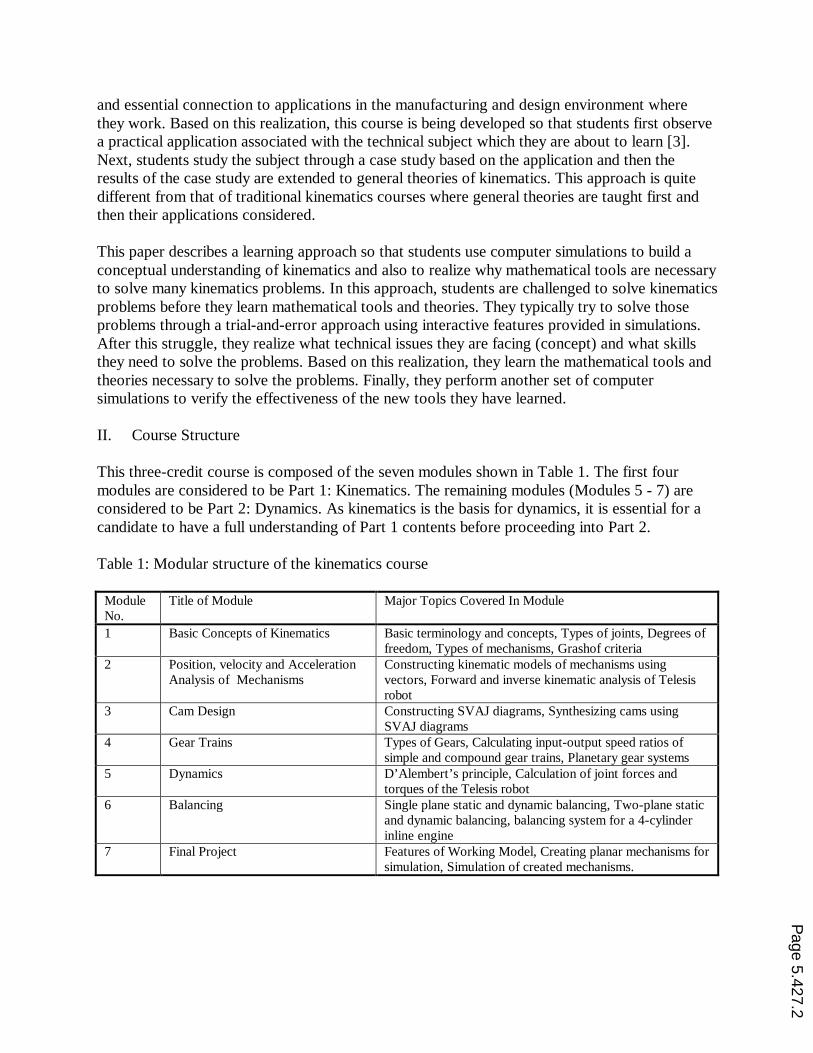
Table 1: Modular structure of the kinematics course

ModuleNo.

Title of Module Major Topics Covered In Module

1 Basic Concepts of Kinematics Basic terminology and concepts, Types of joints, Degrees offreedom, Types of mechanisms, Grashof criteria

2 Position, velocity and AccelerationAnalysis of Mechanisms

Constructing kinematic models of mechanisms usingvectors, Forward and inverse kinematic analysis of Telesisrobot

3 Cam Design Constructing SVAJ diagrams, Synthesizing cams usingSVAJ diagrams

4 Gear Trains Types of Gears, Calculating input-output speed ratios ofsimple and compound gear trains, Planetary gear systems

5 Dynamics D’Alembert’s principle, Calculation of joint forces andtorques of the Telesis robot

6 Balancing Single plane static and dynamic balancing, Two-plane staticand dynamic balancing, balancing system for a 4-cylinderinline engine

7 Final Project Features of Working Model, Creating planar mechanisms forsimulation, Simulation of created mechanisms.

Page 5.427.2

III. Learning Approach

The learning approach for each technical subject in this kinematics course consists of thefollowing five major stages.

1. Observation of practical application

The course development was based on the premise that basic science and engineering principlesare best understood by demonstrating their practical applications. Students will observeoperations of machines through video clips, photos and in some cases see actual operations ofmachines at CAT of Focus:HOPE [3]. The aim here is not to teach technical tools of kinematicsbut to make students realize that a machine they see has a distinctive role in the context of itsintegrated environment such as a manufacturing line. At later stages of the learning process, thisrecognition should become a motivation factor to study the mathematics and science behind themechanism operation.

2. Discovery simulations

Students use computer simulations and manipulate controllable parameters of a mechanism.Discussions among students and between students and an instructor are encouraged to describethe changes they observe by modifying those controllable variables. This is a discovery stage tomake students think about relationship between parameters and outcomes to develop a conceptof a given kinematics issue. Most of computer simulations in this course were developed usingWorking Model. Working Model is a very user friendly software package for designing andanalyzing mechanisms and it has been often used in kinematics education [2,5].

3. Simulations with specified conditions

At this stage, students are asked some specific questions to help solve kinematics problems usingcomputer simulations. Those questions are designed so that students are able to find out if theconcept they developed in the previous stage was appropriate. Also some questions are providedso that students will become frustrated trying to find a right combination of input parameters tosatisfy an output requirement by a mere trial-and-error type approach. Students realize that thereshould be a systematic way to solve a given problem.

4. Learning of technical tools

Students learn the mathematics and science based approach to solve the kinematics problem theystruggled to solve in the simulations.

5. Verification simulations

Students verify effectiveness and validity of kinematics tools they learned in the previous stagethrough a new set of computer simulations.

Page 5.427.3

IV. Examples of Instructional Materials

Example 1: Grashof criteria

The four-bar mechanism is a fundamental linkage mechanism and its applications are found invariety of mechanisms including fixture clamps [3] at Focus:HOPE CAT. Three different kindsof four-bar mechanisms, crank-rocker, double-rocker and double-crank can be generateddepending on how the relative link lengths among four bars are set and which of four links aregrounded. The crank can rotate continuously through 360° while the rocker can rotate only for alimited range of angle less than 360°. This technical issue called Grashof criteria [1] is coveredin Module 1. The computer screen of a simulation to study Grashof criteria is shown in Fig. 1.Scroll bars are provided to change the link length of any of the four bars of the four-barmechanism shown on the left part of the screen. The bottom link of the mechanism is groundedand motion of the mechanism can be generated by installing a motor at a pin joint (Point A orPoint D).

At the stage of "Discovery simulations," each student tries to develop his or her own idea of howparameters provided by those scroll bars could affect the generation of different types of four-barmechanisms. To give students some guidance for exploring their thought, a hint is providedbesides each scroll bar. For example, the top scroll bar is labeled as “Crank Rocker Mechanism,Link 1 – Shortest, Motor – Link1.” After some idea is developed, students are encouraged toexchange their findings using word processors and email bulletin boards. The instructor is alsoencouraged to participate in this discussion to provide appropriate guidance to students. Asmentioned earlier, the aim at this stage is not necessarily to obtain a perfect answer ordescription but to encourage students to build a concept by deriving technical findings from theirobservations.

At the next stage of "Simulations with specified conditions," more specific directions will beprovided to students to come up with technically more mature descriptions and answers. Forexample, to form a crank-rocker mechanism, the shortest link must be located adjacent to thegrounded link. To fully understand this condition, students may be asked to answer a series ofquestions such as

(1) Make Link 1 shortest, run the mechanism to see what type of mechanism resulted.(2) Make Link 2 shortest, run the mechanism to see what type of mechanism resulted.(3) Make Link 3 shortest, run the mechanism to see what type of mechanism resulted.(4) Make Link 4 shortest, run the mechanism to see what type of mechanism resulted.(5) Which cases generated a crank rocker mechanism?(6) From these results, where must the shortest link be placed relative to the grounded link?

Students should find out that only two cases (1) and (3) above result in the crank-rockermechanism, and for these cases, the shortest link is adjacent to the grounded link. After thesesimulations, students study this subject through a kinematics textbook such as [1], to learn usefultechnical tools such as math equations. Authors believe that the experience from computersimulations will greatly help students to master the contents of those technical tools. Afterstudying the textbook, students go back to the computer simulations again to verify the validityof those technical tools they learned.

Page 5.427.4

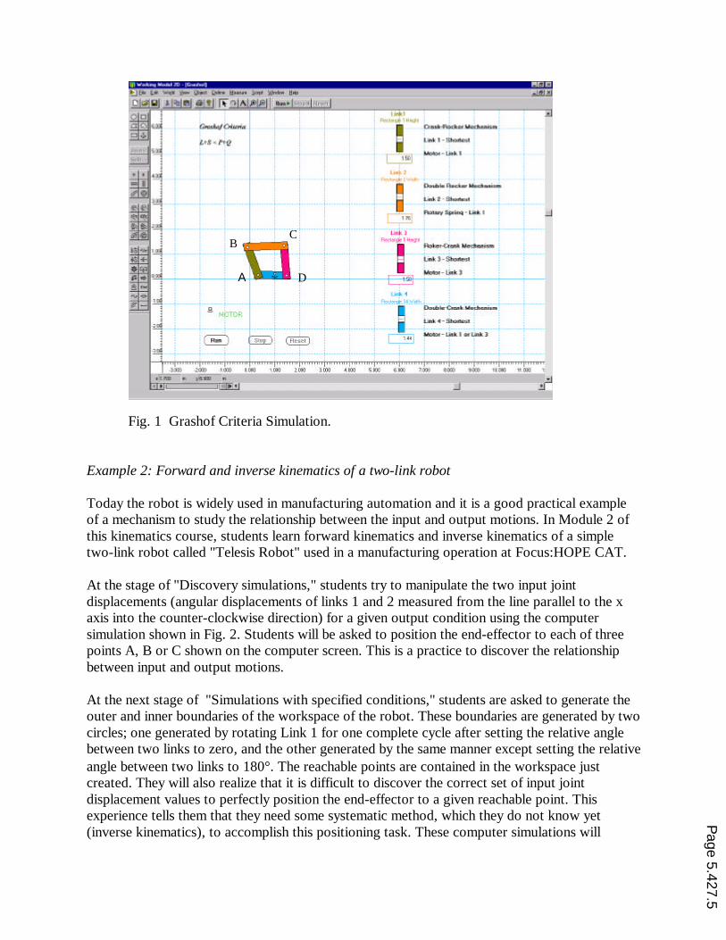
Fig. 1 Grashof Criteria Simulation.

Example 2: Forward and inverse kinematics of a two-link robot

Today the robot is widely used in manufacturing automation and it is a good practical exampleof a mechanism to study the relationship between the input and output motions. In Module 2 ofthis kinematics course, students learn forward kinematics and inverse kinematics of a simpletwo-link robot called "Telesis Robot" used in a manufacturing operation at Focus:HOPE CAT.

At the stage of "Discovery simulations," students try to manipulate the two input jointdisplacements (angular displacements of links 1 and 2 measured from the line parallel to the xaxis into the counter-clockwise direction) for a given output condition using the computersimulation shown in Fig. 2. Students will be asked to position the end-effector to each of threepoints A, B or C shown on the computer screen. This is a practice to discover the relationshipbetween input and output motions.

At the next stage of "Simulations with specified conditions," students are asked to generate theouter and inner boundaries of the workspace of the robot. These boundaries are generated by twocircles; one generated by rotating Link 1 for one complete cycle after setting the relative anglebetween two links to zero, and the other generated by the same manner except setting the relativeangle between two links to 180°. The reachable points are contained in the workspace justcreated. They will also realize that it is difficult to discover the correct set of input jointdisplacement values to perfectly position the end-effector to a given reachable point. Thisexperience tells them that they need some systematic method, which they do not know yet(inverse kinematics), to accomplish this positioning task. These computer simulations will

A

BC

D

Page 5.427.5

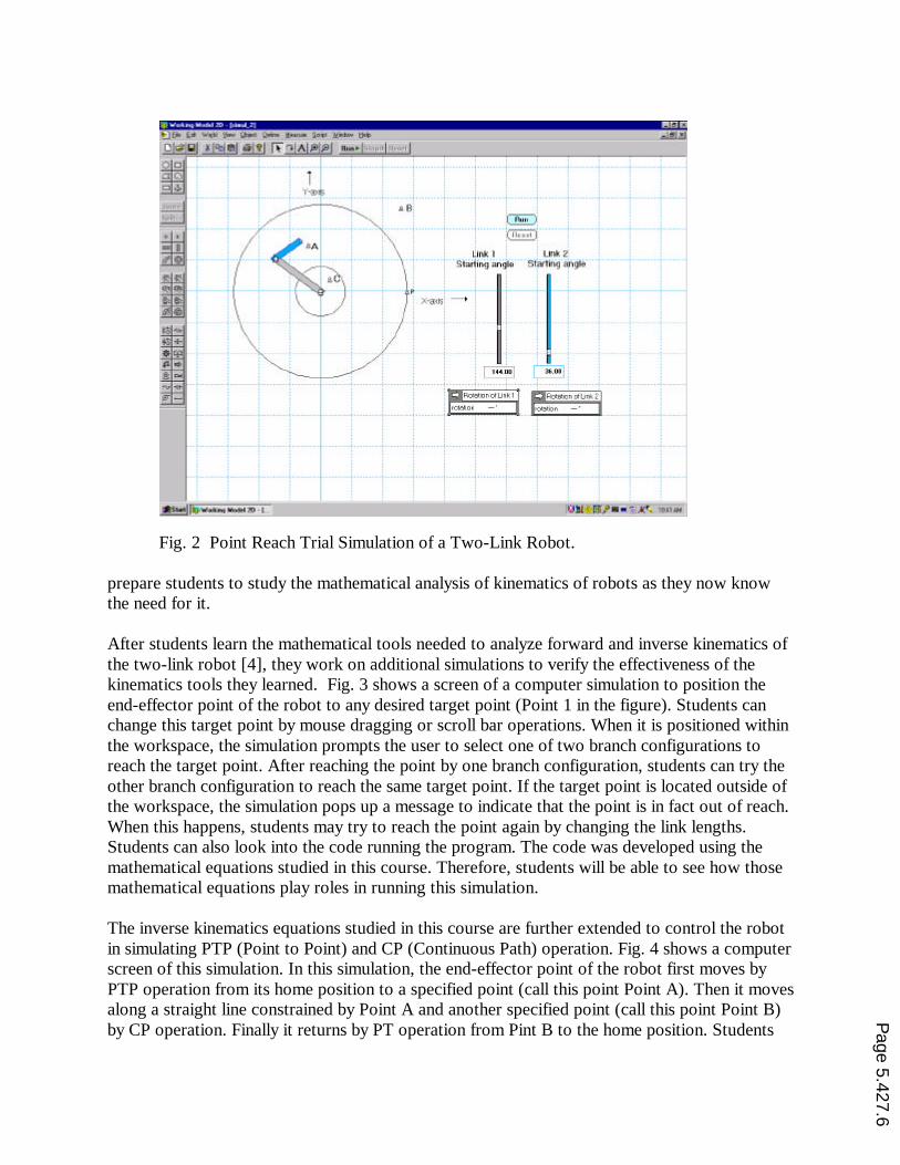
Fig. 2 Point Reach Trial Simulation of a Two-Link Robot.

prepare students to study the mathematical analysis of kinematics of robots as they now knowthe need for it.

After students learn the mathematical tools needed to analyze forward and inverse kinematics ofthe two-link robot [4], they work on additional simulations to verify the effectiveness of thekinematics tools they learned. Fig. 3 shows a screen of a computer simulation to position theend-effector point of the robot to any desired target point (Point 1 in the figure). Students canchange this target point by mouse dragging or scroll bar operations. When it is positioned withinthe workspace, the simulation prompts the user to select one of two branch configurations toreach the target point. After reaching the point by one branch configuration, students can try theother branch configuration to reach the same target point. If the target point is located outside ofthe workspace, the simulation pops up a message to indicate that the point is in fact out of reach.When this happens, students may try to reach the point again by changing the link lengths.Students can also look into the code running the program. The code was developed using themathematical equations studied in this course. Therefore, students will be able to see how thosemathematical equations play roles in running this simulation.

The inverse kinematics equations studied in this course are further extended to control the robotin simulating PTP (Point to Point) and CP (Continuous Path) operation. Fig. 4 shows a computerscreen of this simulation. In this simulation, the end-effector point of the robot first moves byPTP operation from its home position to a specified point (call this point Point A). Then it movesalong a straight line constrained by Point A and another specified point (call this point Point B)by CP operation. Finally it returns by PT operation from Pint B to the home position. Students

Page 5.427.6

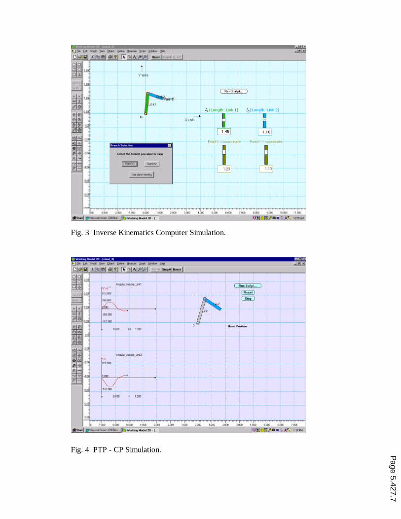
Fig. 3 Inverse Kinematics Computer Simulation.

Fig. 4 PTP - CP Simulation. Page 5.427.7

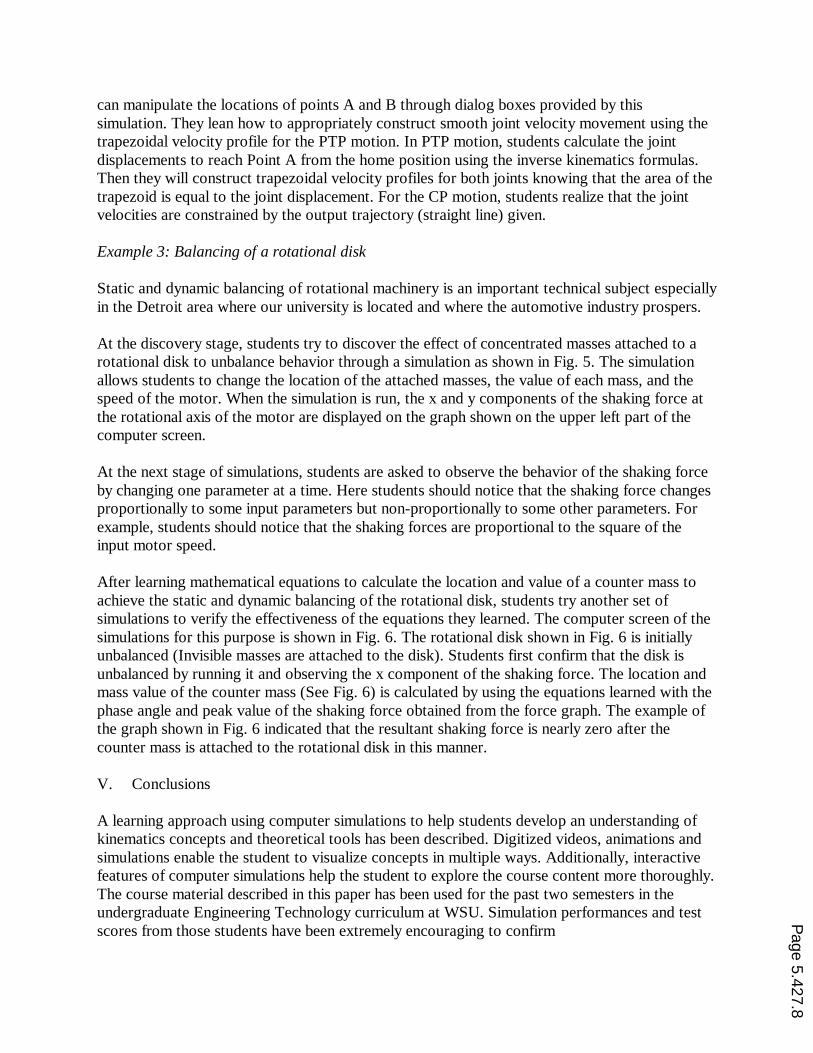
can manipulate the locations of points A and B through dialog boxes provided by thissimulation. They lean how to appropriately construct smooth joint velocity movement using thetrapezoidal velocity profile for the PTP motion. In PTP motion, students calculate the jointdisplacements to reach Point A from the home position using the inverse kinematics formulas.Then they will construct trapezoidal velocity profiles for both joints knowing that the area of thetrapezoid is equal to the joint displacement. For the CP motion, students realize that the jointvelocities are constrained by the output trajectory (straight line) given.

Example 3: Balancing of a rotational disk

Static and dynamic balancing of rotational machinery is an important technical subject especiallyin the Detroit area where our university is located and where the automotive industry prospers.

At the discovery stage, students try to discover the effect of concentrated masses attached to arotational disk to unbalance behavior through a simulation as shown in Fig. 5. The simulationallows students to change the location of the attached masses, the value of each mass, and thespeed of the motor. When the simulation is run, the x and y components of the shaking force atthe rotational axis of the motor are displayed on the graph shown on the upper left part of thecomputer screen.

At the next stage of simulations, students are asked to observe the behavior of the shaking forceby changing one parameter at a time. Here students should notice that the shaking force changesproportionally to some input parameters but non-proportionally to some other parameters. Forexample, students should notice that the shaking forces are proportional to the square of theinput motor speed.

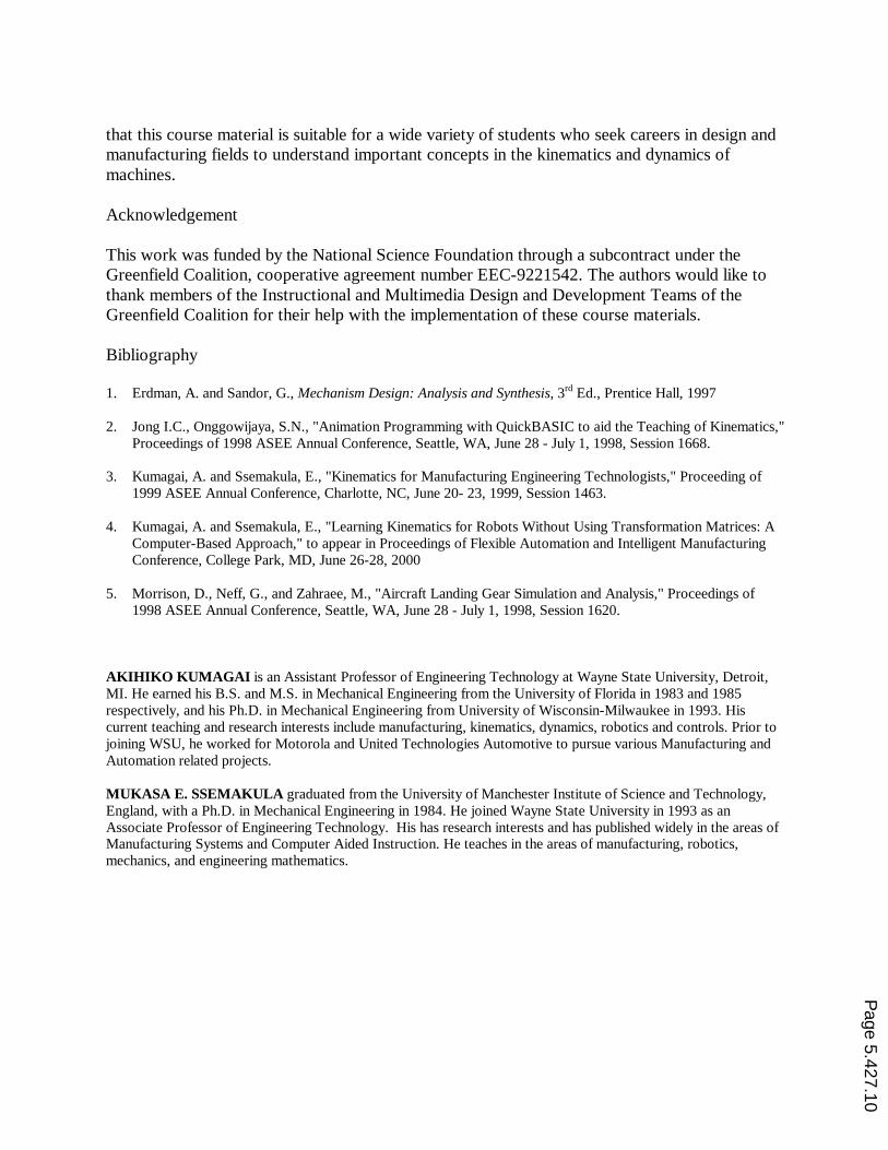
After learning mathematical equations to calculate the location and value of a counter mass toachieve the static and dynamic balancing of the rotational disk, students try another set ofsimulations to verify the effectiveness of the equations they learned. The computer screen of thesimulations for this purpose is shown in Fig. 6. The rotational disk shown in Fig. 6 is initiallyunbalanced (Invisible masses are attached to the disk). Students first confirm that the disk isunbalanced by running it and observing the x component of the shaking force. The location andmass value of the counter mass (See Fig. 6) is calculated by using the equations learned with thephase angle and peak value of the shaking force obtained from the force graph. The example ofthe graph shown in Fig. 6 indicated that the resultant shaking force is nearly zero after thecounter mass is attached to the rotational disk in this manner.

V. Conclusions

A learning approach using computer simulations to help students develop an understanding ofkinematics concepts and theoretical tools has been described. Digitized videos, animations andsimulations enable the student to visualize concepts in multiple ways. Additionally, interactivefeatures of computer simulations help the student to explore the course content more thoroughly.The course material described in this paper has been used for the past two semesters in theundergraduate Engineering Technology curriculum at WSU. Simulation performances and testscores from those students have been extremely encouraging to confirm

Page 5.427.8

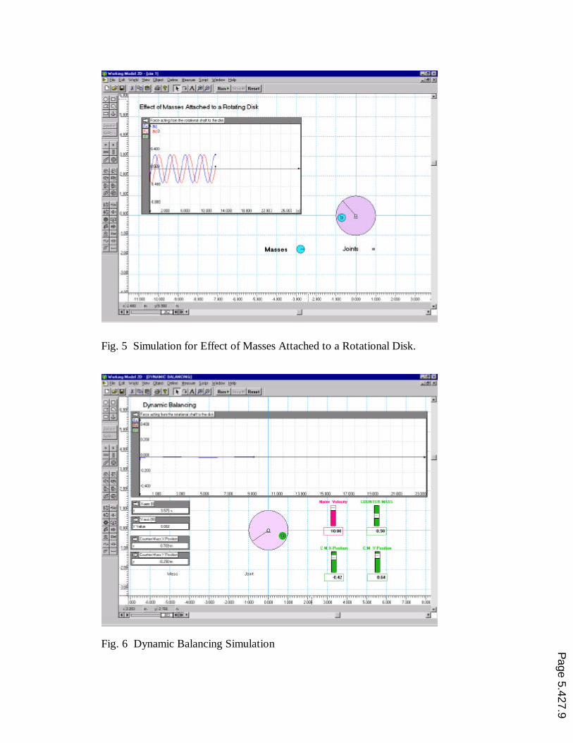
Fig. 5 Simulation for Effect of Masses Attached to a Rotational Disk.

Fig. 6 Dynamic Balancing Simulation Page 5.427.9

that this course material is suitable for a wide variety of students who seek careers in design andmanufacturing fields to understand important concepts in the kinematics and dynamics ofmachines.

Acknowledgement

This work was funded by the National Science Foundation through a subcontract under theGreenfield Coalition, cooperative agreement number EEC-9221542. The authors would like tothank members of the Instructional and Multimedia Design and Development Teams of theGreenfield Coalition for their help with the implementation of these course materials.

Bibliography

1. Erdman, A. and Sandor, G., Mechanism Design: Analysis and Synthesis, 3rd Ed., Prentice Hall, 1997

2. Jong I.C., Onggowijaya, S.N., "Animation Programming with QuickBASIC to aid the Teaching of Kinematics,"Proceedings of 1998 ASEE Annual Conference, Seattle, WA, June 28 - July 1, 1998, Session 1668.

3. Kumagai, A. and Ssemakula, E., "Kinematics for Manufacturing Engineering Technologists," Proceeding of1999 ASEE Annual Conference, Charlotte, NC, June 20- 23, 1999, Session 1463.

4. Kumagai, A. and Ssemakula, E., "Learning Kinematics for Robots Without Using Transformation Matrices: AComputer-Based Approach," to appear in Proceedings of Flexible Automation and Intelligent ManufacturingConference, College Park, MD, June 26-28, 2000

5. Morrison, D., Neff, G., and Zahraee, M., "Aircraft Landing Gear Simulation and Analysis," Proceedings of1998 ASEE Annual Conference, Seattle, WA, June 28 - July 1, 1998, Session 1620.

AKIHIKO KUMAGAI is an Assistant Professor of Engineering Technology at Wayne State University, Detroit,MI. He earned his B.S. and M.S. in Mechanical Engineering from the University of Florida in 1983 and 1985respectively, and his Ph.D. in Mechanical Engineering from University of Wisconsin-Milwaukee in 1993. Hiscurrent teaching and research interests include manufacturing, kinematics, dynamics, robotics and controls. Prior tojoining WSU, he worked for Motorola and United Technologies Automotive to pursue various Manufacturing andAutomation related projects.

MUKASA E. SSEMAKULA graduated from the University of Manchester Institute of Science and Technology,England, with a Ph.D. in Mechanical Engineering in 1984. He joined Wayne State University in 1993 as anAssociate Professor of Engineering Technology. His has research interests and has published widely in the areas ofManufacturing Systems and Computer Aided Instruction. He teaches in the areas of manufacturing, robotics,mechanics, and engineering mathematics.

Page 5.427.10