Lecture 13. Clinical studies andLecture 13. Clinical studies and basic biostatistics

ME330.884 “Mass spectrometry in an ‘omics’ world”December 10, 2012,

1Stefani Thomas, Ph.D.

Statistics and biostatistics

• Statistics collection organization analysis• Statistics – collection, organization, analysis, and interpretation of numerical data

• Objective: make an inference about a population based on information contained in a sample

• Biostatistics – application of statistical methods to medical and biological problems

2

Role of statistics in decision-making processesprocesses

A l i f d t f li i l t i l t d t i• Analysis of data from clinical trials to determine efficacy of new drugs

• Should a mastectomy always be recommended to a patient with breast cancer?to a patient with breast cancer?

Wh t f t i th i k th t i di id l• What factors increase the risk that an individual will develop coronary heart disease?

3

Numbers are more precise than wordsp

• “There are three kinds of lies: lies, damned lies, and statistics” – Benjamin Disraeli (British Primeand statistics – Benjamin Disraeli (British Prime Minister 1874 - 1880)

• “It is easy to lie with statistics, but it is easier to lie without them” – Professor Frederick Mosteller(founding chairman of Harvard’s statistics department, 1956)

4

1. Types of data (variables)2 Descriptive statistics/Numerical summary2. Descriptive statistics/Numerical summary

measures3 Measures of dispersion/variability3. Measures of dispersion/variability4. Normal distribution and confidence intervals5 Hypothesis testing5. Hypothesis testing6. Correlation and regression analysis7 Analysis of variance (ANOVA)7. Analysis of variance (ANOVA)8. Experimental design

5

1. Types of data (variables)yp ( )

6

Categorical datag

• Nominal data - categories without a natural dorder

– Sex, race, country

• Ordinal data – categories with a natural order– e g Socioeconomic status (low middle high); type of bonee.g., Socioeconomic status (low, middle, high); type of bone

break (hairline, simple, compound)– Numbers can be assigned to specific values, but the value of the

numbers is arbitrarynumbers is arbitrary

• % and proportions are used to analyze

7

ycategorical data

Discrete data

• Ordered numerical data restricted to integer valuesvalues– e.g., Number of deaths due to AIDS in 2011; eggs laid per

chicken; number of new cases of tuberculosis reported in the U S during a one year periodU.S. during a one-year period

– Both ordering and magnitude are important– Numbers represent actual measurable quantities rather than

l b lmere labels

8

Continuous data

• Ordered numerical data that can theoretically take on any value• Ordered numerical data that can theoretically take on any value

• Data that represent measurable quantities but are not restricted to taking on certain specified values (such as integers)

• Only limiting factor for a continuous observation is the degree• Only limiting factor for a continuous observation is the degree of accuracy with which it can be measured

• e.g., serum cholesterol level of a patient, concentration of a pollutant, height, weight, age, temperature

9

2. Descriptive statistics/numerical summary measures

10

Measures of central tendencyy

• Most commonly investigated characteristic of a set of data is its• Most commonly investigated characteristic of a set of data is its center, or the point about which the observations tend to cluster

11

Mean

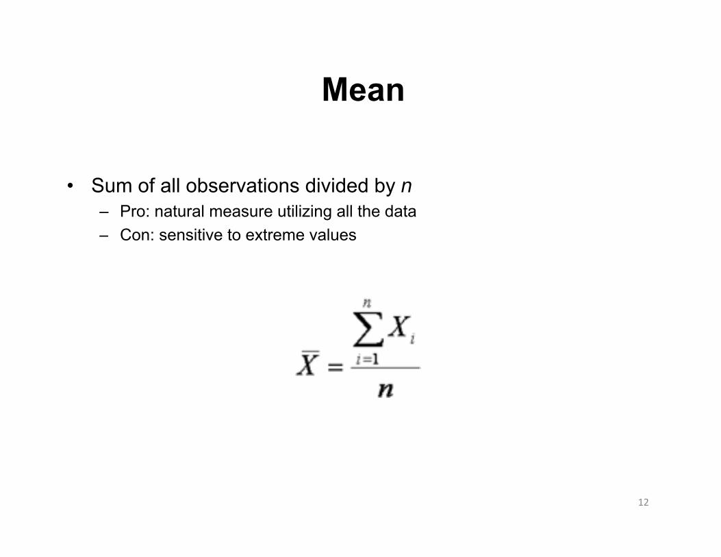
• Sum of all observations divided by n– Pro: natural measure utilizing all the data– Con: sensitive to extreme values

12

Median (m)( )

• Middle-most observation of ordered data– Pro: insensitive to extreme values– Con: determined mainly by middle points of sampley y p p

• Calculation1 Order data from smallest to largest1. Order data from smallest to largest2. If n is odd: m = (n+1)/2 largest observation3. If n is even: m = average of the (n/2) and (n/2) +1

observation

13

Mode

• Observation that occurs most frequently– Pro: can be used with categorical data (e.g., most popular

presidential candidate)p )– Con: less useful with continuous data

• Possible for data set to not have any modes or more than 1Possible for data set to not have any modes or more than 1 mode

14

Relationshipsp

• Symmetric distribution: mean = median = mode• Symmetric distribution: mean = median = mode

• Skewed distribution“t th i ht” di– “to the right”: mean>median

– “to the left”: mean<median

15

3. Measures of dispersion/variability

16

Rangeg

• Difference between the largest observation and the smallest• Quick and dirty measure of variability

– Pro: easy to calculate– Pro: easy to calculate– Cons:

• Sensitive to extreme valuesT d t i ith i i• Tends to increase with increasing n

17

Interquartile rangeq g

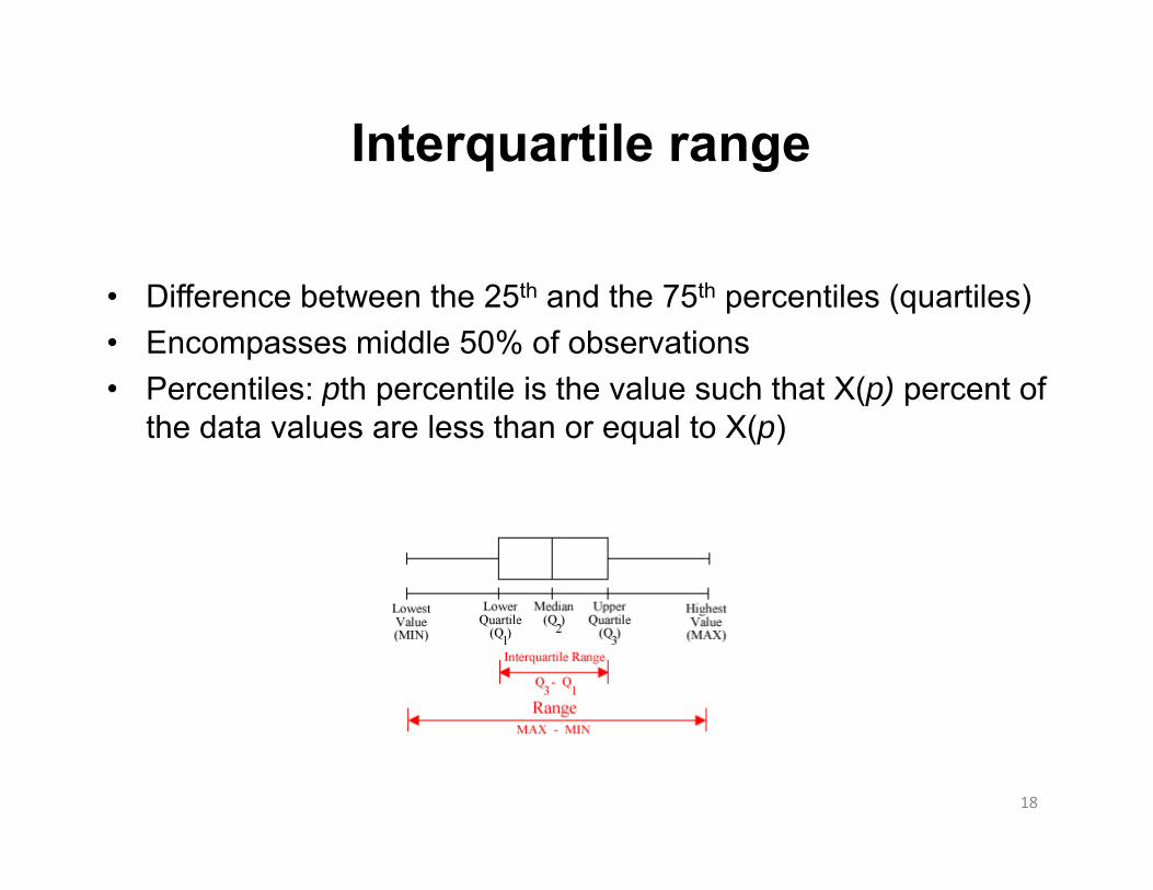
• Difference between the 25th and the 75th percentiles (quartiles)• Encompasses middle 50% of observations• Percentiles: pth percentile is the value such that X(p) percent of• Percentiles: pth percentile is the value such that X(p) percent of

the data values are less than or equal to X(p)

18

Variance

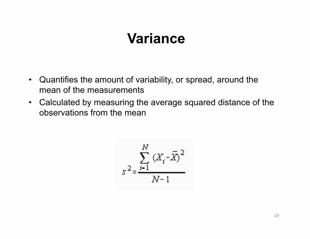
• Quantifies the amount of variability, or spread, around the mean of the measurements

• Calculated by measuring the average squared distance of theCalculated by measuring the average squared distance of the observations from the mean

19

Standard deviation

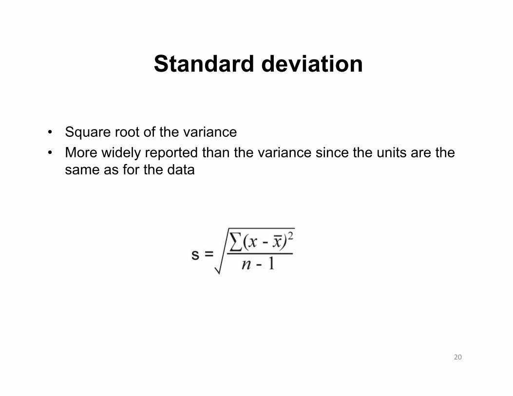
• Square root of the variance• More widely reported than the variance since the units are the

same as for the datasame as for the data

20

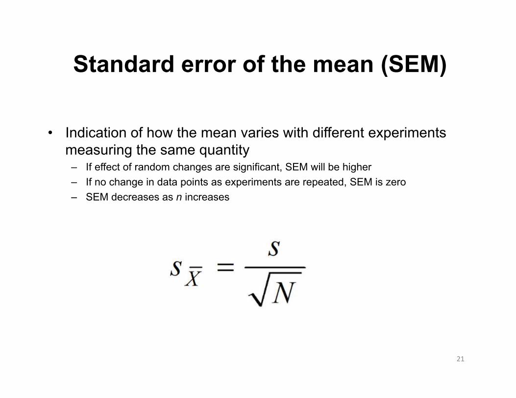
Standard error of the mean (SEM)( )

• Indication of how the mean varies with different experiments measuring the same quantity

– If effect of random changes are significant, SEM will be higher– If no change in data points as experiments are repeated, SEM is zero– SEM decreases as n increases

21

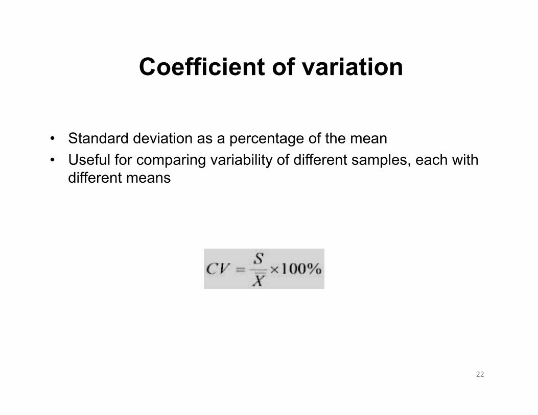
Coefficient of variation

• Standard deviation as a percentage of the mean• Useful for comparing variability of different samples, each with

different meansdifferent means

22

4. Normal distribution and confidence intervals

23

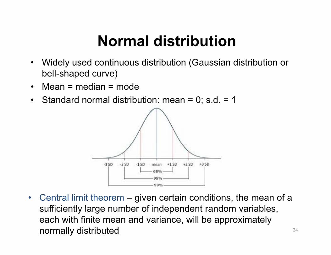
Normal distribution• Widely used continuous distribution (Gaussian distribution or

bell-shaped curve)• Mean = median = mode• Standard normal distribution: mean = 0; s.d. = 1

• Central limit theorem – given certain conditions, the mean of a sufficiently large number of independent random variables

24

sufficiently large number of independent random variables, each with finite mean and variance, will be approximately normally distributed

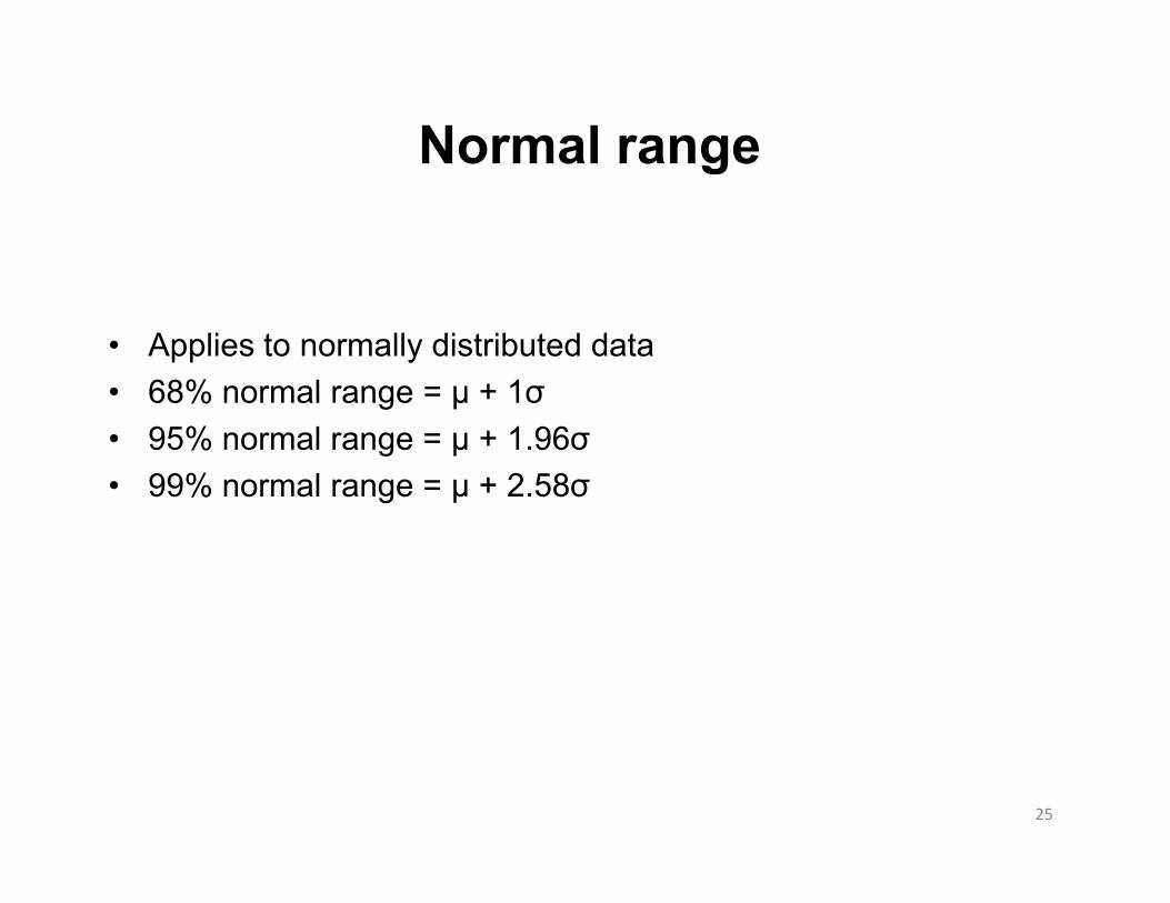
Normal rangeg

• Applies to normally distributed data• 68% normal range = µ + 1σ• 68% normal range = µ + 1σ• 95% normal range = µ + 1.96σ• 99% normal range = µ + 2.58σ

25

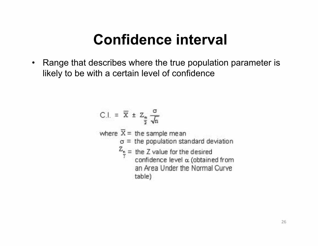
Confidence interval• Range that describes where the true population parameter is

likely to be with a certain level of confidencey

26

5 Hypothesis testing5. Hypothesis testing

27

Procedure for hypothesis testingyp g

• Hypothesis testing - an objective framework for making scientific conclusions based on a samplemaking scientific conclusions based on a sample of data

28

Procedure for hypothesis testing:Step 1Step 1

• Ask a question about a population parameterq p p p– Is the mean CD4 count for HIV(+) patients less than 400?– Does smoking increase the risk of lung cancer?

Is there a difference in mean serum cholesterol levels between– Is there a difference in mean serum cholesterol levels between kids who eat oatmeal and kids who eat Frosted Cheerios?

29

Procedure for hypothesis testing:Step 2Step 2

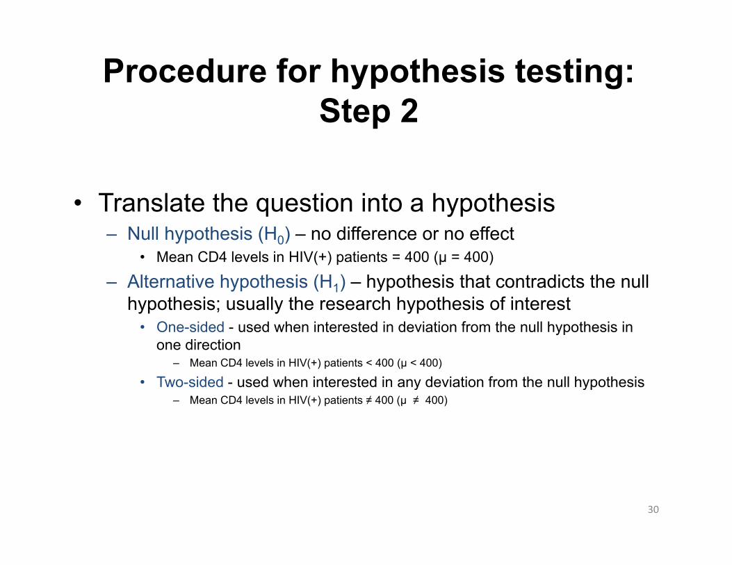
• Translate the question into a hypothesis– Null hypothesis (H0) – no difference or no effect

• Mean CD4 levels in HIV(+) patients = 400 (µ = 400)

– Alternative hypothesis (H1) – hypothesis that contradicts the null hypothesis; usually the research hypothesis of interest

• One-sided - used when interested in deviation from the null hypothesis in one direction

– Mean CD4 levels in HIV(+) patients < 400 (µ < 400)

• Two-sided - used when interested in any deviation from the null hypothesisy yp– Mean CD4 levels in HIV(+) patients ≠ 400 (µ ≠ 400)

30

Procedure for hypothesis testing:Step 3Step 3

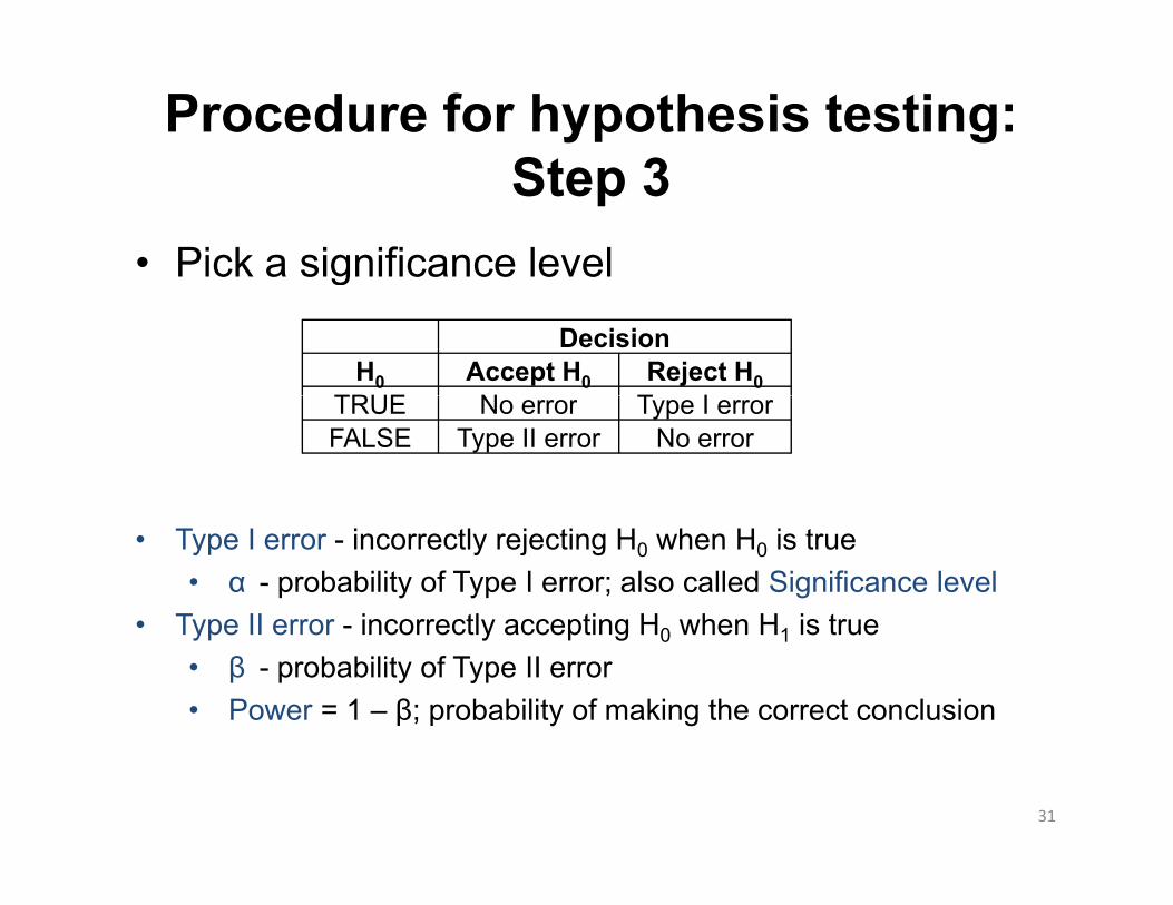
• Pick a significance levelg

DecisionH0 Accept H0 Reject H0

TRUE N T ITRUE No error Type I errorFALSE Type II error No error

• Type I error - incorrectly rejecting H0 when H0 is true • α - probability of Type I error; also called Significance level

• Type II error incorrectly accepting H when H is true• Type II error - incorrectly accepting H0 when H1 is true • β - probability of Type II error• Power = 1 – β; probability of making the correct conclusion

31

Procedure for hypothesis testing:Steps 4 7Steps 4 - 7

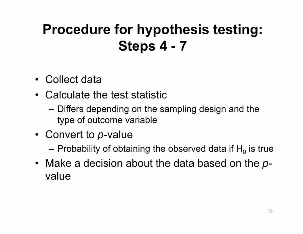
• Collect data• Calculate the test statistic

– Differs depending on the sampling design and the type of outcome variable

C t t l• Convert to p-value– Probability of obtaining the observed data if H0 is true

Make a decision about the data based on the p• Make a decision about the data based on the p-value

32

Test statistics for inferences about a pop lation meanpopulation mean

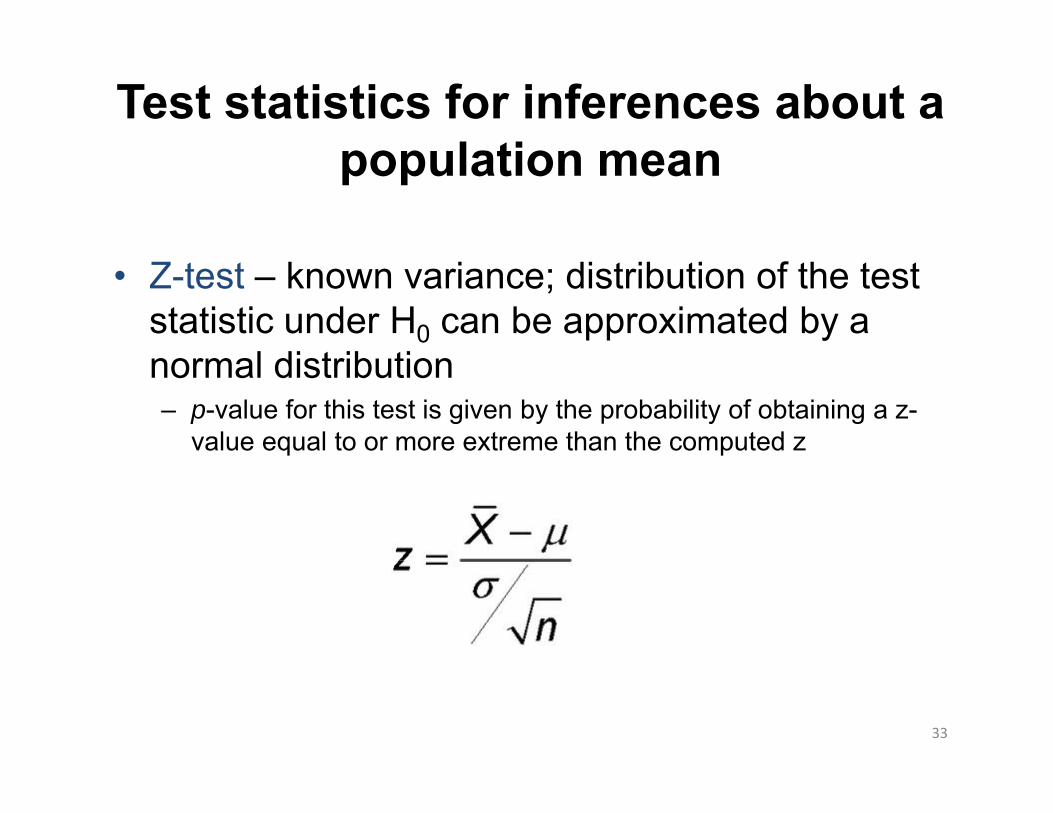
• Z-test – known variance; distribution of the test statistic under H0 can be approximated by a

l di t ib tinormal distribution– p-value for this test is given by the probability of obtaining a z-

value equal to or more extreme than the computed z

33

Test statistics for inferences about a pop lation meanpopulation mean

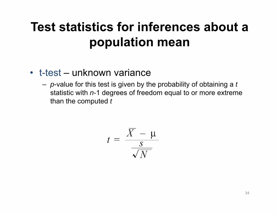
• t-test – unknown variance– p-value for this test is given by the probability of obtaining a t

statistic with n-1 degrees of freedom equal to or more extremestatistic with n 1 degrees of freedom equal to or more extreme than the computed t

34

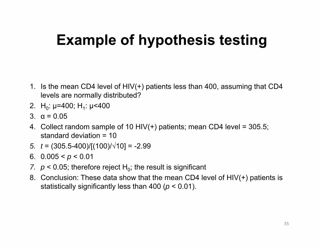
Example of hypothesis testingp yp g

1. Is the mean CD4 level of HIV(+) patients less than 400, assuming that CD4 levels are normally distributed?

2. H0: µ=400; H1: µ<4000 µ ; 1 µ3. α = 0.054. Collect random sample of 10 HIV(+) patients; mean CD4 level = 305.5;

standard deviation = 105. t = (305.5-400)/[(100)/√10] = -2.996. 0.005 < p < 0.017. p < 0.05; therefore reject H0; the result is significantj 0 g8. Conclusion: These data show that the mean CD4 level of HIV(+) patients is

statistically significantly less than 400 (p < 0.01).

35

6. Correlation and regression analysis

36

Correlation

• Quantification of the degree to which two random i bl l t d id d th t th l ti hi ivariables are related, provided that the relationship is

linear• AdvantagesAdvantages

– Maintain continuity of data– Model one variable as a function of the other

Di d• Disadvantages– Only measures linear relationships– Requires normality assumption for testing hypothesesq y p g yp– Only useful when both variables are continuous

37

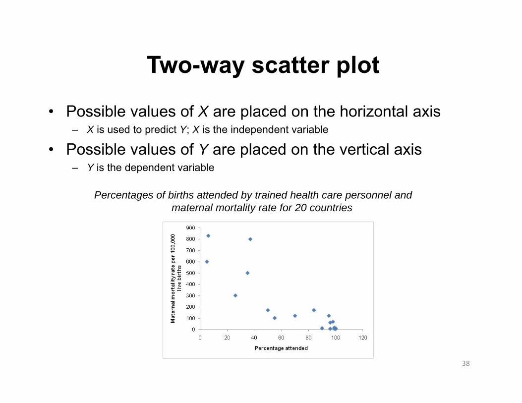
Two-way scatter ploty p

• Possible values of X are placed on the horizontal axis– X is used to predict Y; X is the independent variable

• Possible values of Y are placed on the vertical axis– Y is the dependent variable

Percentages of births attended by trained health care personnel and maternal mortality rate for 20 countries

38

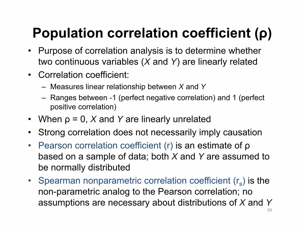
Population correlation coefficient (ρ)• Purpose of correlation analysis is to determine whether

two continuous variables (X and Y) are linearly relatedC l ti ffi i t• Correlation coefficient:– Measures linear relationship between X and Y– Ranges between -1 (perfect negative correlation) and 1 (perfect

positive correlation)

• When ρ = 0, X and Y are linearly unrelated• Strong correlation does not necessarily imply causation• Strong correlation does not necessarily imply causation• Pearson correlation coefficient (r) is an estimate of ρ

based on a sample of data; both X and Y are assumed to p ;be normally distributed

• Spearman nonparametric correlation coefficient (rs) is the non parametric analog to the Pearson correlation; no

39

non-parametric analog to the Pearson correlation; no assumptions are necessary about distributions of X and Y

Simple linear regressionp g

• Purpose is to model the change in Y as X changes• Examples of uses:

– Prediction (what is the predicted amount of time it will take you to get home from work given the time that you leave?)get home from work given the time that you leave?)

– Linear association (is there a linear relationship between CD4 levels and time since infection with HIV?)

40

7. Analysis of variance (ANOVA)

41

ANOVA

• Used to model the means of one variable (Y) for the various• Used to model the means of one variable (Y) for the various levels of other variables

• Extension of the two-sample t-test to three or more samples• Number of t-tests increases geometrically as a function of the

number of groups; analysis becomes cognitively difficult; ANOVA organizes and directs the analysisg y

• Conducting a greater number of analyses greatly increases the probability of committing at least one Type I error somewhere in the analysisthe analysis

• Performing fewer hypothesis tests reduces the experimental error rate

42

Completely randomized design;One a ANOVAOne-way ANOVA

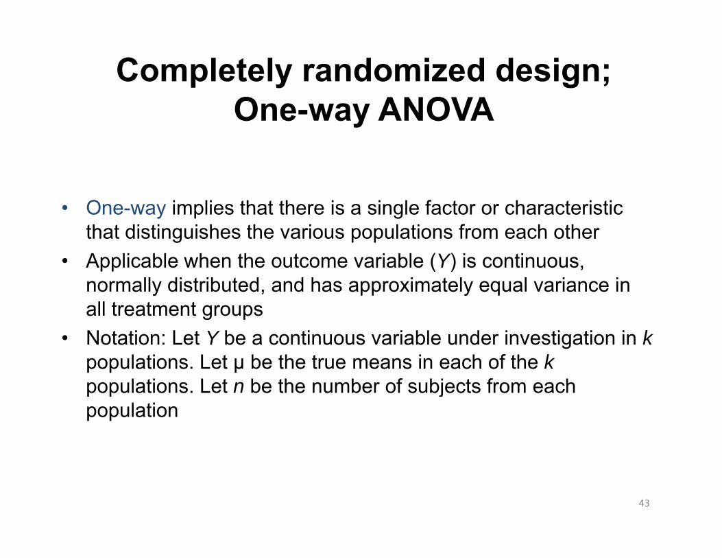
• One-way implies that there is a single factor or characteristic that distinguishes the various populations from each other

• Applicable when the outcome variable (Y) is continuous, normally distributed, and has approximately equal variance in all treatment groupsall treatment groups

• Notation: Let Y be a continuous variable under investigation in k populations. Let µ be the true means in each of the k populations Let n be the number of subjects from eachpopulations. Let n be the number of subjects from each population

43

Completely randomized design;One a ANOVA

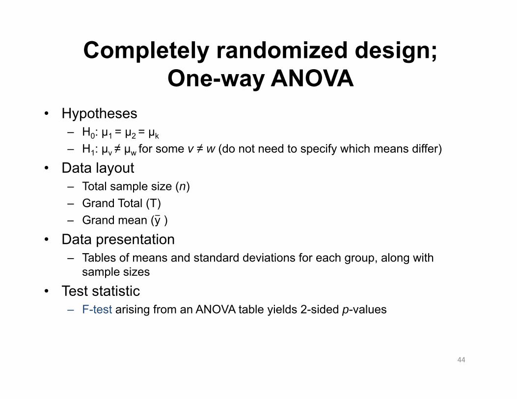
• Hypotheses

One-way ANOVA

– H0: µ1 = µ2 = µk

– H1: µv ≠ µw for some v ≠ w (do not need to specify which means differ)

• Data layouty– Total sample size (n)– Grand Total (T)– Grand mean (y )(y )

• Data presentation– Tables of means and standard deviations for each group, along with

sample sizessample sizes

• Test statistic– F-test arising from an ANOVA table yields 2-sided p-values

44

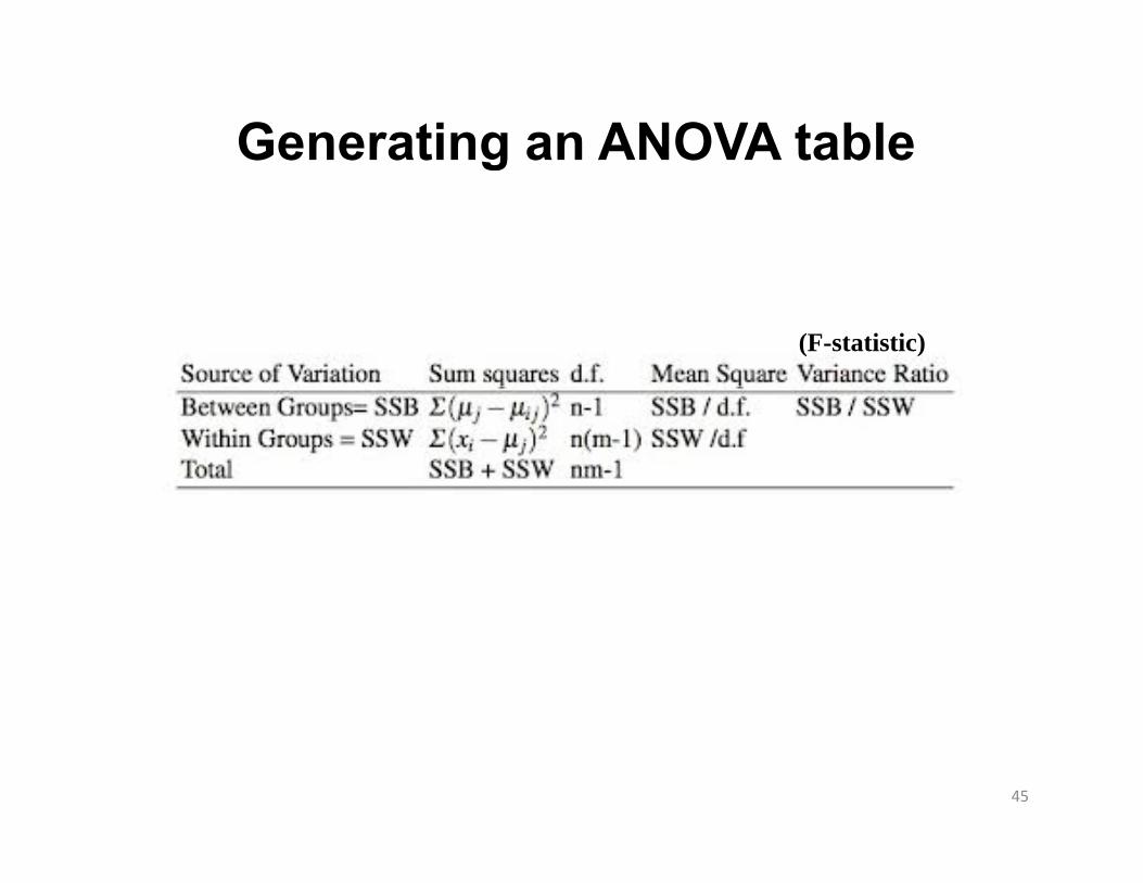
Generating an ANOVA tableg

(F-statistic)

45

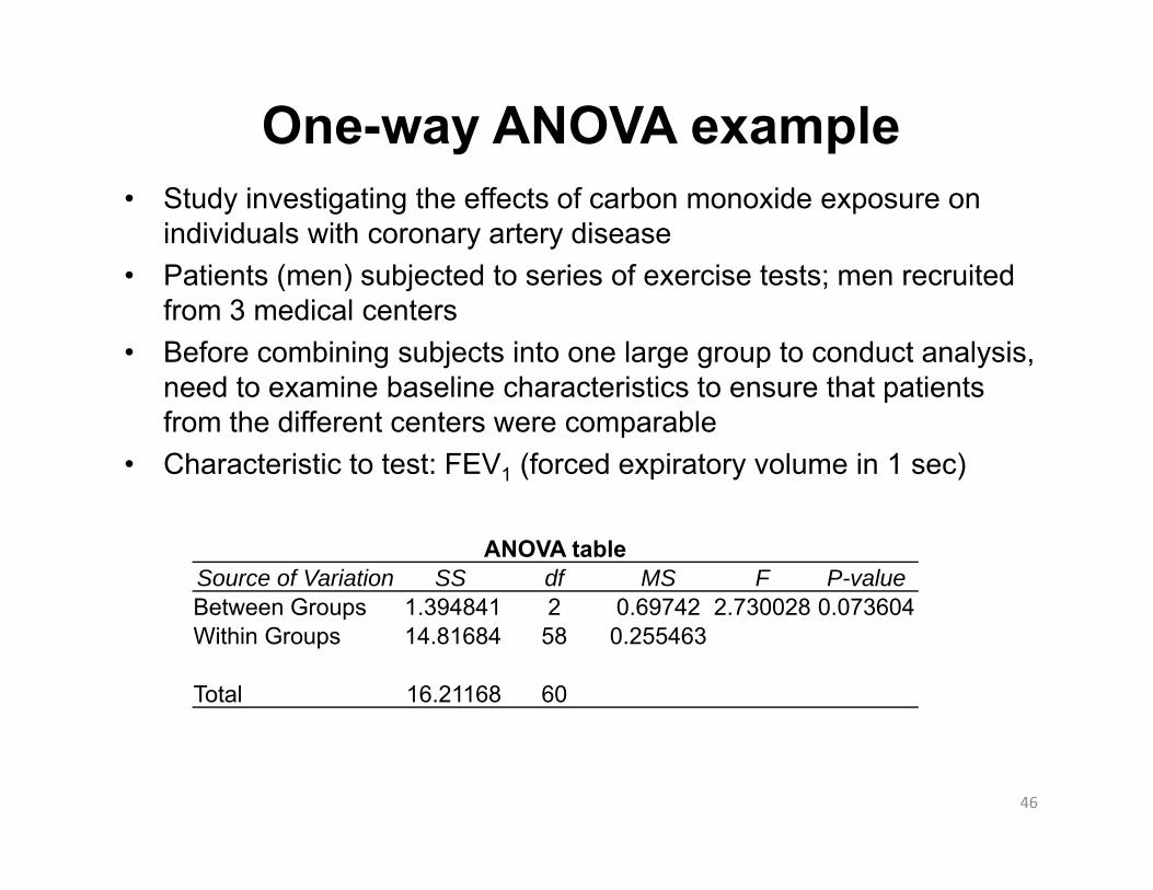
One-way ANOVA example• Study investigating the effects of carbon monoxide exposure on

individuals with coronary artery disease• Patients (men) subjected to series of exercise tests; men recruited• Patients (men) subjected to series of exercise tests; men recruited

from 3 medical centers• Before combining subjects into one large group to conduct analysis,

need to examine baseline characteristics to ensure that patientsneed to examine baseline characteristics to ensure that patients from the different centers were comparable

• Characteristic to test: FEV1 (forced expiratory volume in 1 sec)

ANOVA tableSource of Variation SS df MS F P-valueBetween Groups 1.394841 2 0.69742 2.730028 0.073604Between Groups 1.394841 2 0.69742 2.730028 0.073604Within Groups 14.81684 58 0.255463

Total 16.21168 60

46

8 Experimental design8. Experimental design

47

Sample size determinationp

• When designing a study with the goal of testing a hypothesis, we need to know how many subjects to study

• Five variables must be specified• Five variables must be specified1. α: level of significance2. One- or two-sided form of alternative hypothesis3. δ: desired difference to detect4. Power: 1 – β (probability of detecting a difference of δ; power

increases with increasing sample size)5. σD: standard deviation of the paired differences (typically

estimated using published or pilot data)

48

Basic study designs(listed in order of increasing stringency)1 Cross-sectional study

y g

1. Cross sectional study– observation of a population, or a representative subset, at one

specific point in timedescriptive study (not longitudinal or experimental)– descriptive study (not longitudinal or experimental)

2. Cohort (prospective/observational) study– identify cohort; measure exposure; follow for prolonged period of

ti d t i h d l di l t d t itime; determine who develops disease; analyze to determine whether disease is associated with exposure

3. Case-control (retrospective) study– identify set of patients with disease and corresponding set of

controls without disease; find out retrospectively about exposure; analyze data to determine whether associations exist

49