Lecture 3: Major hydrologic models-HSPF, HEC and MIKE · HEC-HMS Background. Purpose of HEC -HMS Improved User Interface, Graphics, and Reporting Improved Hydrologic Computations

Lecture 3: Major hydrologic models-HSPF, HEC and MIKE

Module 9

Major Hydrologic Models

HSPF (SWM)

HEC

MIKE

Module 9

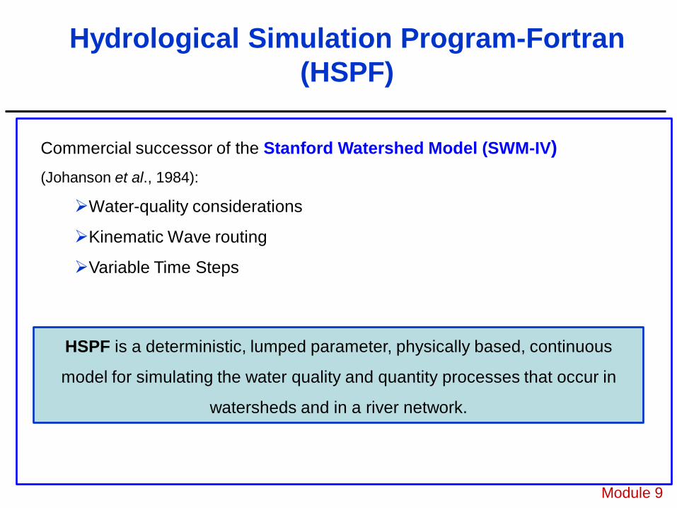
HSPF is a deterministic, lumped parameter, physically based, continuous

model for simulating the water quality and quantity processes that occur in

watersheds and in a river network.

Commercial successor of the Stanford Watershed Model (SWM-IV) (Johanson et al., 1984):

Water-quality considerations

Kinematic Wave routing

Variable Time Steps

Module 9

Hydrological Simulation Program-Fortran (HSPF)

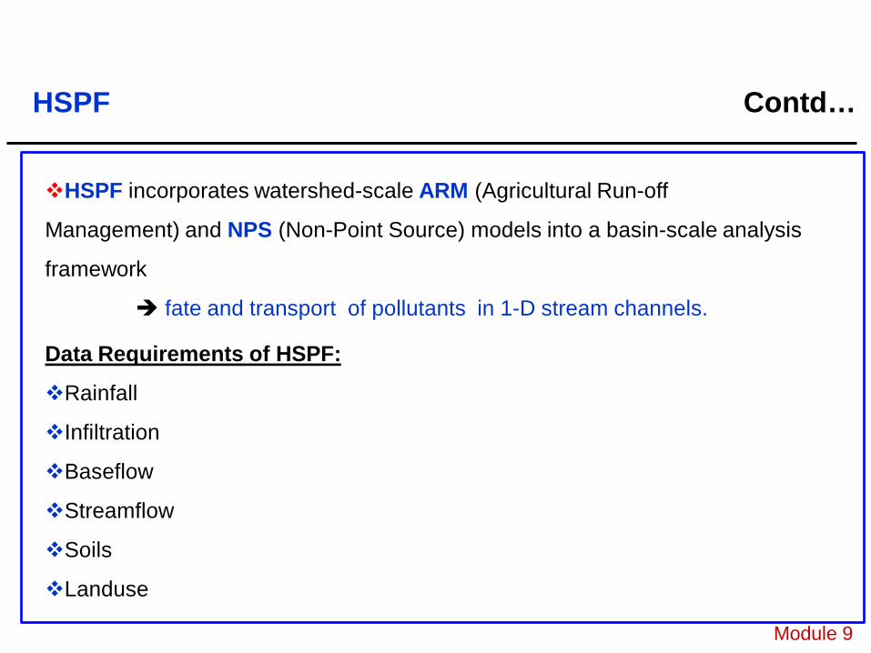
Data Requirements of HSPF:

Rainfall

Infiltration

Baseflow

Streamflow

Soils

Landuse

HSPF incorporates watershed-scale ARM (Agricultural Run-off

Management) and NPS (Non-Point Source) models into a basin-scale analysis

framework

fate and transport of pollutants in 1-D stream channels.

Module 9

HSPF Contd…

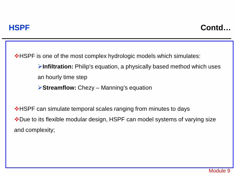
HSPF is one of the most complex hydrologic models which simulates:

Infiltration: Philip's equation, a physically based method which uses

an hourly time step

Streamflow: Chezy – Manning’s equation

HSPF can simulate temporal scales ranging from minutes to days

Due to its flexible modular design, HSPF can model systems of varying size

and complexity;

Module 9

HSPF Contd…

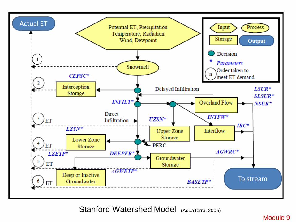
Stanford Watershed Model (AquaTerra, 2005)

To stream

Actual ET

Output

1

Module 9

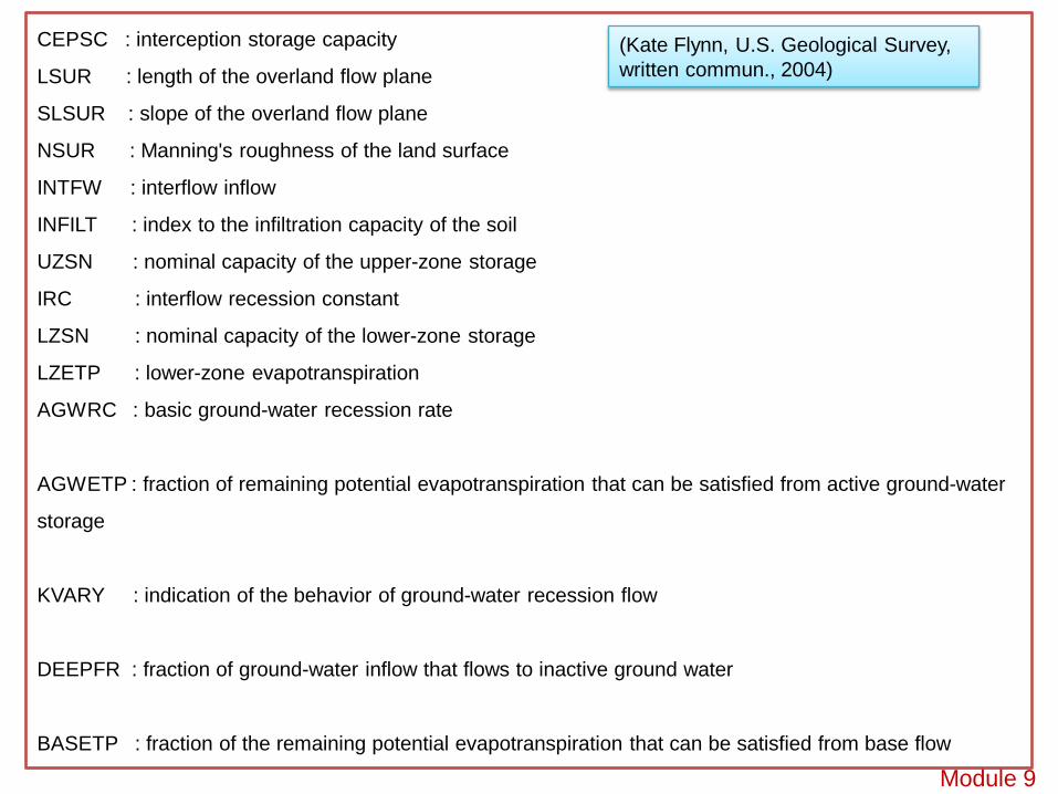
CEPSC : interception storage capacity

LSUR : length of the overland flow plane

SLSUR : slope of the overland flow plane

NSUR : Manning's roughness of the land surface

INTFW : interflow inflow

INFILT : index to the infiltration capacity of the soil

UZSN : nominal capacity of the upper-zone storage

IRC : interflow recession constant

LZSN : nominal capacity of the lower-zone storage

LZETP : lower-zone evapotranspiration

AGWRC : basic ground-water recession rate

AGWETP : fraction of remaining potential evapotranspiration that can be satisfied from active ground-water

storage

KVARY : indication of the behavior of ground-water recession flow

DEEPFR : fraction of ground-water inflow that flows to inactive ground water

BASETP : fraction of the remaining potential evapotranspiration that can be satisfied from base flow

(Kate Flynn, U.S. Geological Survey, written commun., 2004)

Module 9

HEC Models

Module 9

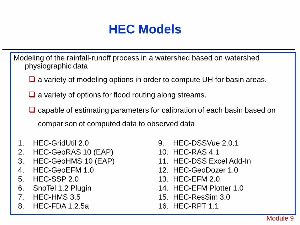
HEC Models

Modeling of the rainfall-runoff process in a watershed based on watershed physiographic data

a variety of modeling options in order to compute UH for basin areas.

a variety of options for flood routing along streams.

capable of estimating parameters for calibration of each basin based on

comparison of computed data to observed data

Module 9

1. HEC-GridUtil 2.02. HEC-GeoRAS 10 (EAP) 3. HEC-GeoHMS 10 (EAP) 4. HEC-GeoEFM 1.0 5. HEC-SSP 2.0 6. SnoTel 1.2 Plugin7. HEC-HMS 3.5 8. HEC-FDA 1.2.5a

9. HEC-DSSVue 2.0.1 10. HEC-RAS 4.1 11. HEC-DSS Excel Add-In 12. HEC-GeoDozer 1.0 13. HEC-EFM 2.0 14. HEC-EFM Plotter 1.0 15. HEC-ResSim 3.0 16. HEC-RPT 1.1

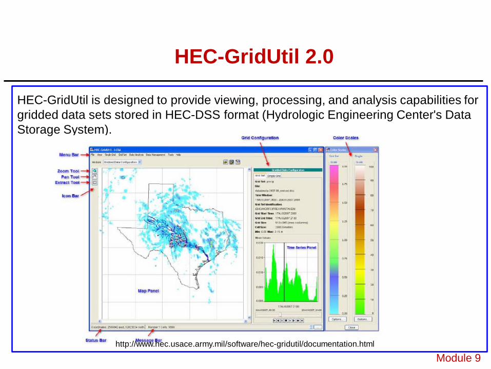
HEC-GridUtil is designed to provide viewing, processing, and analysis capabilities for gridded data sets stored in HEC-DSS format (Hydrologic Engineering Center's Data Storage System).

http://www.hec.usace.army.mil/software/hec-gridutil/documentation.html

HEC-GridUtil 2.0

Module 9

HEC-GeoRAS

Module 9

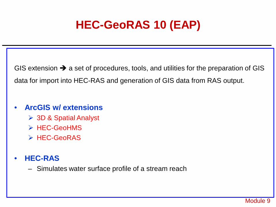
GIS extension a set of procedures, tools, and utilities for the preparation of GIS

data for import into HEC-RAS and generation of GIS data from RAS output.

HEC-GeoRAS 10 (EAP)

• ArcGIS w/ extensions 3D & Spatial Analyst HEC-GeoHMS HEC-GeoRAS

• HEC-RAS– Simulates water surface profile of a stream reach

Module 9

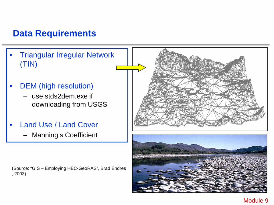
Data Requirements

• Triangular Irregular Network (TIN)

• DEM (high resolution)– use stds2dem.exe if

downloading from USGS

• Land Use / Land Cover– Manning’s Coefficient

Module 9

CRWR image, Texas University

(Source: “GIS – Employing HEC-GeoRAS”, Brad Endres, 2003)

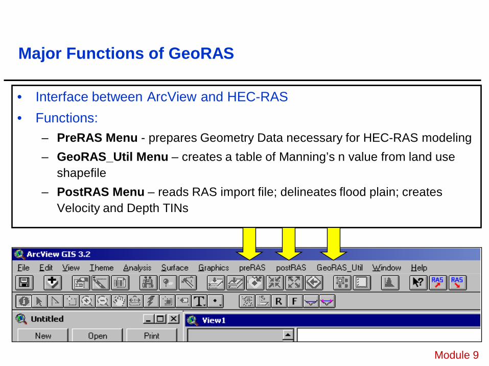
Major Functions of GeoRAS

• Interface between ArcView and HEC-RAS• Functions:

– PreRAS Menu - prepares Geometry Data necessary for HEC-RAS modeling– GeoRAS_Util Menu – creates a table of Manning’s n value from land use

shapefile– PostRAS Menu – reads RAS import file; delineates flood plain; creates

Velocity and Depth TINs

Module 9

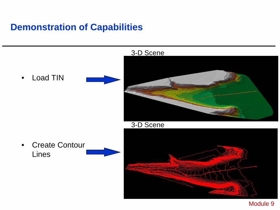
Demonstration of Capabilities

• Load TIN

• Create Contour Lines

Module 9

3-D Scene

3-D Scene

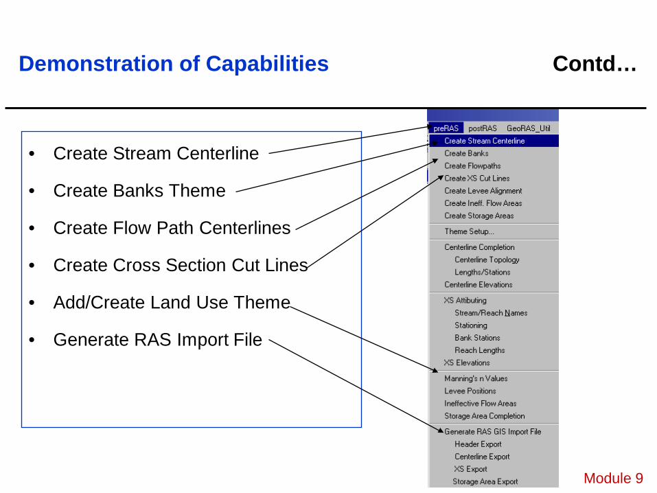
Demonstration of Capabilities Contd…

• Create Stream Centerline

• Create Banks Theme

• Create Flow Path Centerlines

• Create Cross Section Cut Lines

• Add/Create Land Use Theme

• Generate RAS Import File

Module 9

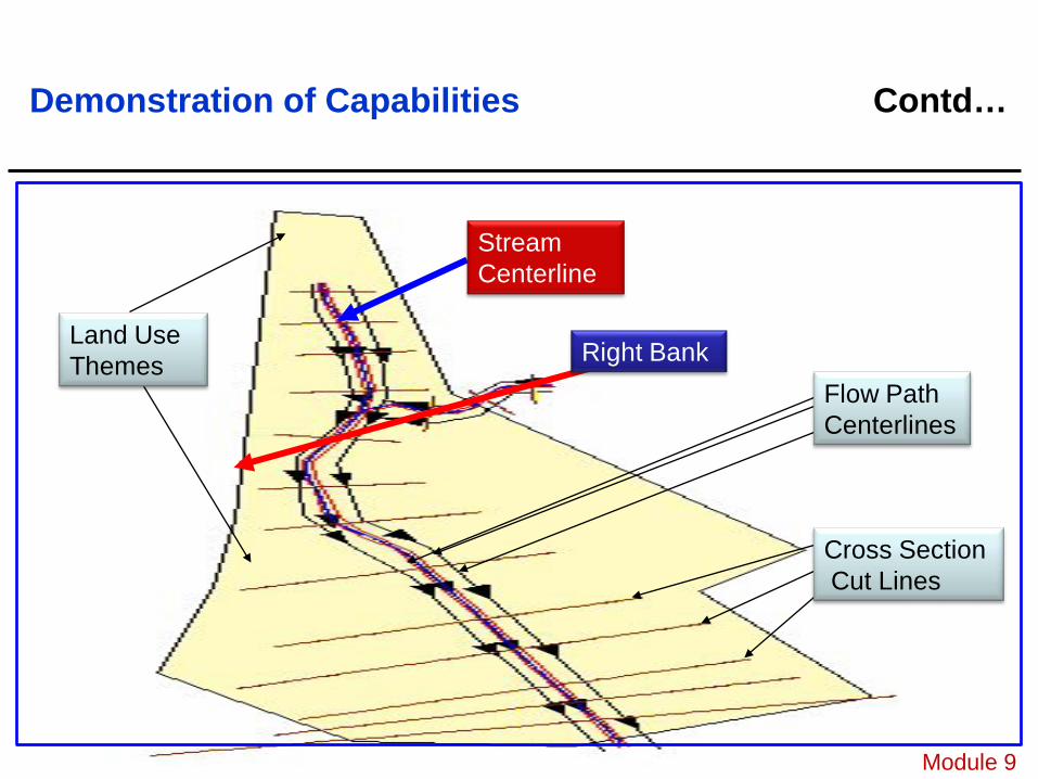
Stream Centerline

Right BankFlow Path Centerlines

Land Use Themes

Cross SectionCut Lines

Module 9


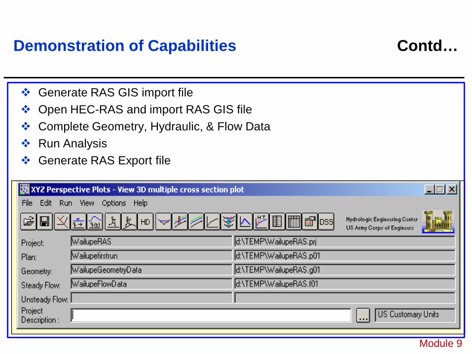
Generate RAS GIS import file Open HEC-RAS and import RAS GIS file Complete Geometry, Hydraulic, & Flow Data Run Analysis Generate RAS Export file

Module 9


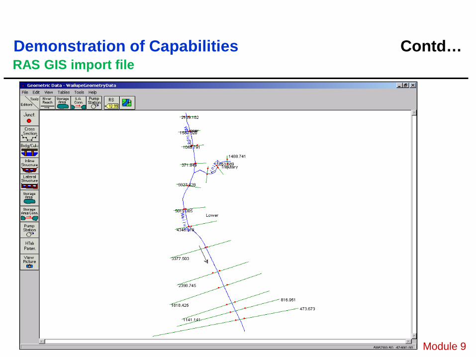
RAS GIS import file

Module 9


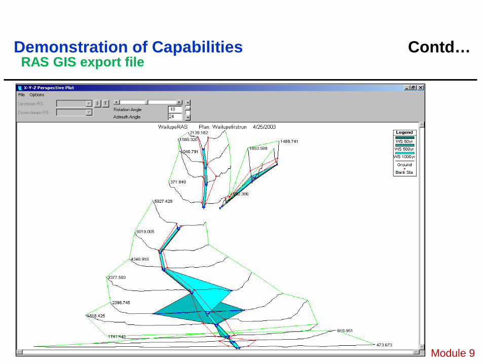
RAS GIS export file

Module 9


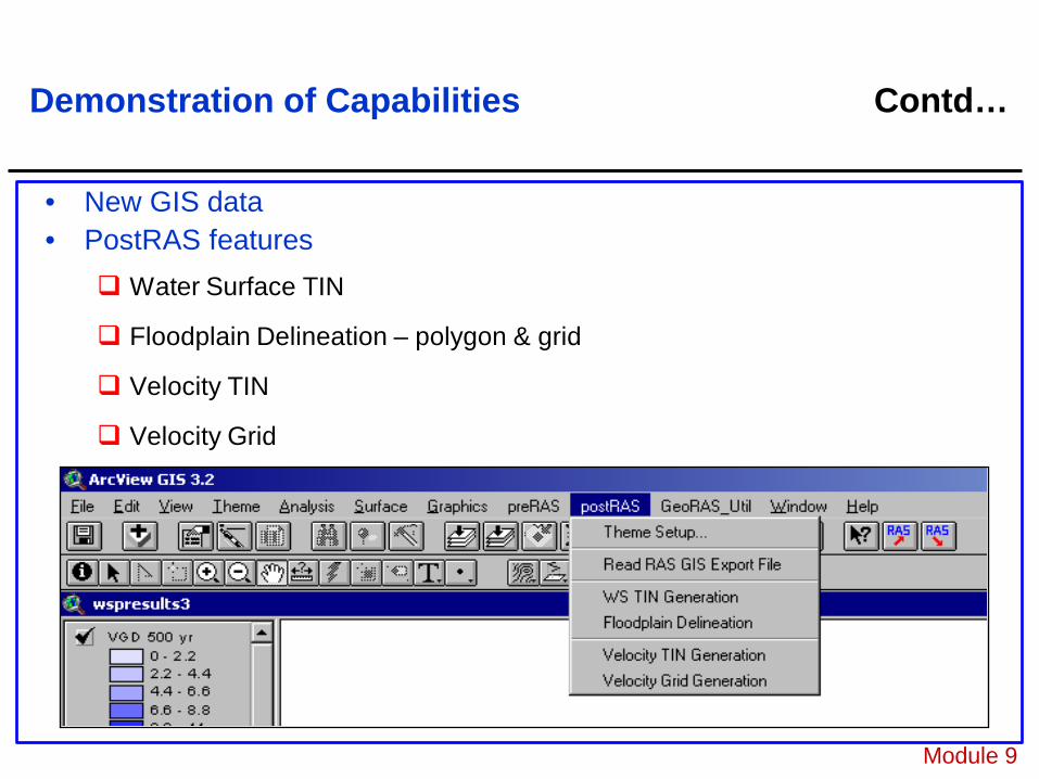
• New GIS data• PostRAS features

Water Surface TIN

Floodplain Delineation – polygon & grid

Velocity TIN

Velocity Grid

Module 9


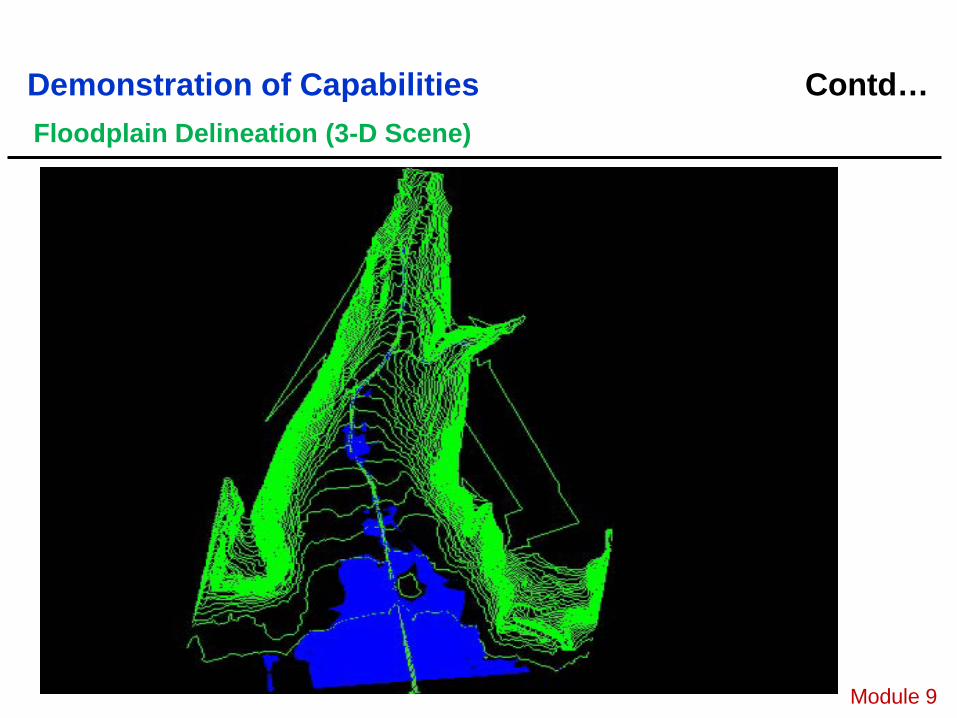
Floodplain Delineation (3-D Scene)

Module 9


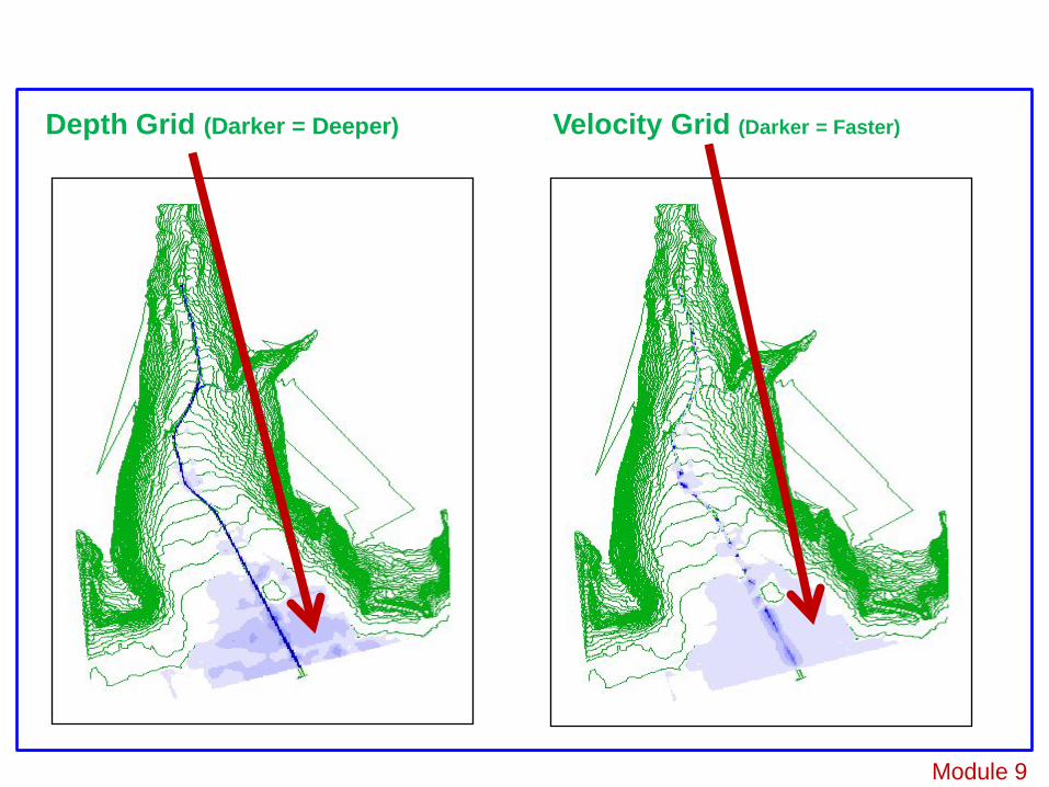
Depth Grid (Darker = Deeper) Velocity Grid (Darker = Faster)

Module 9

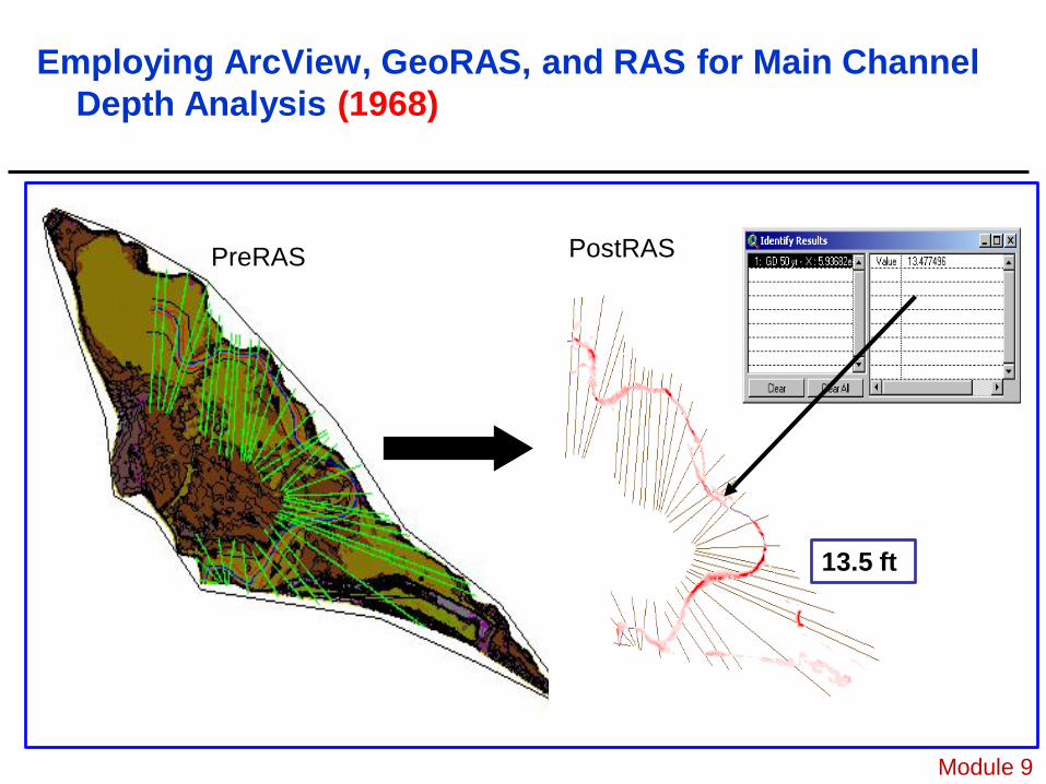
Employing ArcView, GeoRAS, and RAS for Main Channel Depth Analysis (1968)

Module 9

PreRAS PostRAS

13.5 ft

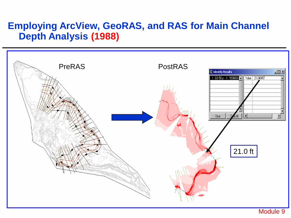
Employing ArcView, GeoRAS, and RAS for Main Channel Depth Analysis (1988)

PreRAS PostRAS

21.0 ft

Module 9

Overall Benefits

Elevation data is more accurate with TIN files

Better representation of channel bottom

Rapid preparation of geometry data (point and click)

Precision of GIS data increases precision of geometry data

Efficient data transport via import/export files

Velocity grid

Depth grid

Module 9

Floodplain maps can be made faster

• several flow scenarios

Both steady & unsteady flow analysis

GIS tools aid engineering analysis• Automated calculation of functions (Energy Equation)• Structural validation of hydraulic control features• Voluminous data on World Wide Web

Makes data into visual event – easier for human brain to process!

Module 9

Overall Benefits Contd…

Overall Drawbacks

Time required to learn several software packages

Non-availability of TIN or high resolution data

Estimation of Manning’s Coefficient• Few LU/LC files have this as attribute data

Velocity distribution data may not be calculated• HEC-RAS export file without velocity data means no velocity TIN or

grid

Module 9

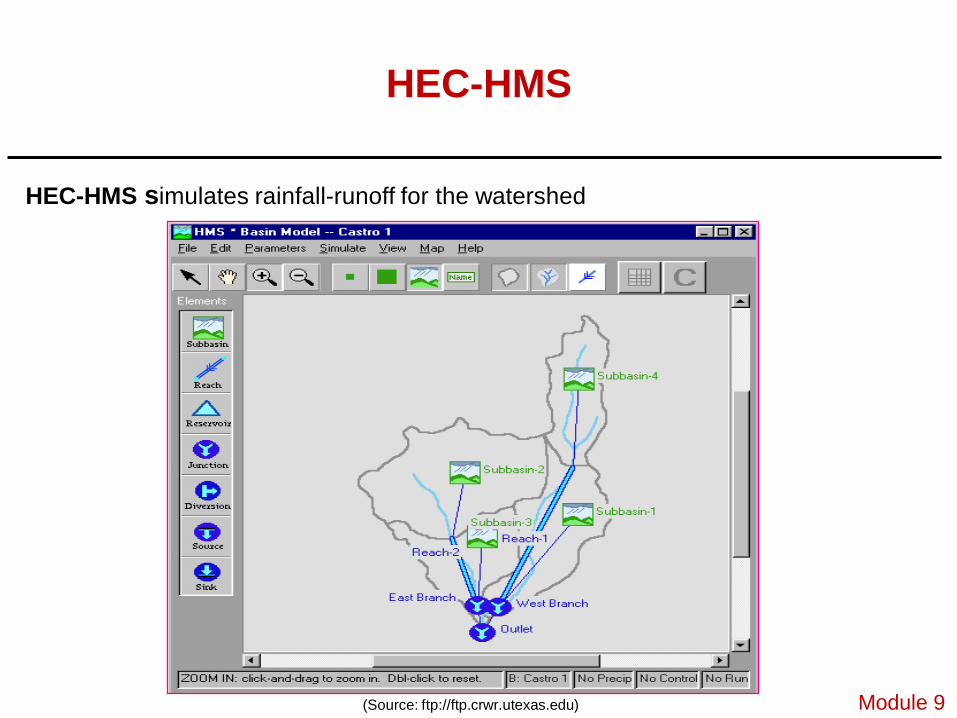
HEC-HMS

HEC-HMS simulates rainfall-runoff for the watershed

(Source: ftp://ftp.crwr.utexas.edu) Module 9

HEC-HMS Background

Purpose of HEC-HMS

Improved User Interface, Graphics, and Reporting

Improved Hydrologic Computations

Integration of Related Hydrologic Capabilities

Importance of HEC-HMS

Foundation for Future Hydrologic Software

Replacement for HEC-1

Module 9

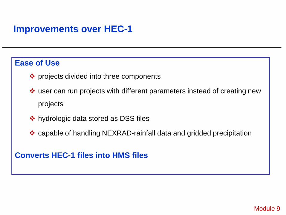
Ease of Use projects divided into three components

user can run projects with different parameters instead of creating new

projects

hydrologic data stored as DSS files

capable of handling NEXRAD-rainfall data and gridded precipitation

Converts HEC-1 files into HMS files

Module 9

Improvements over HEC-1

HEC-1 EXERCISE PROBLEM

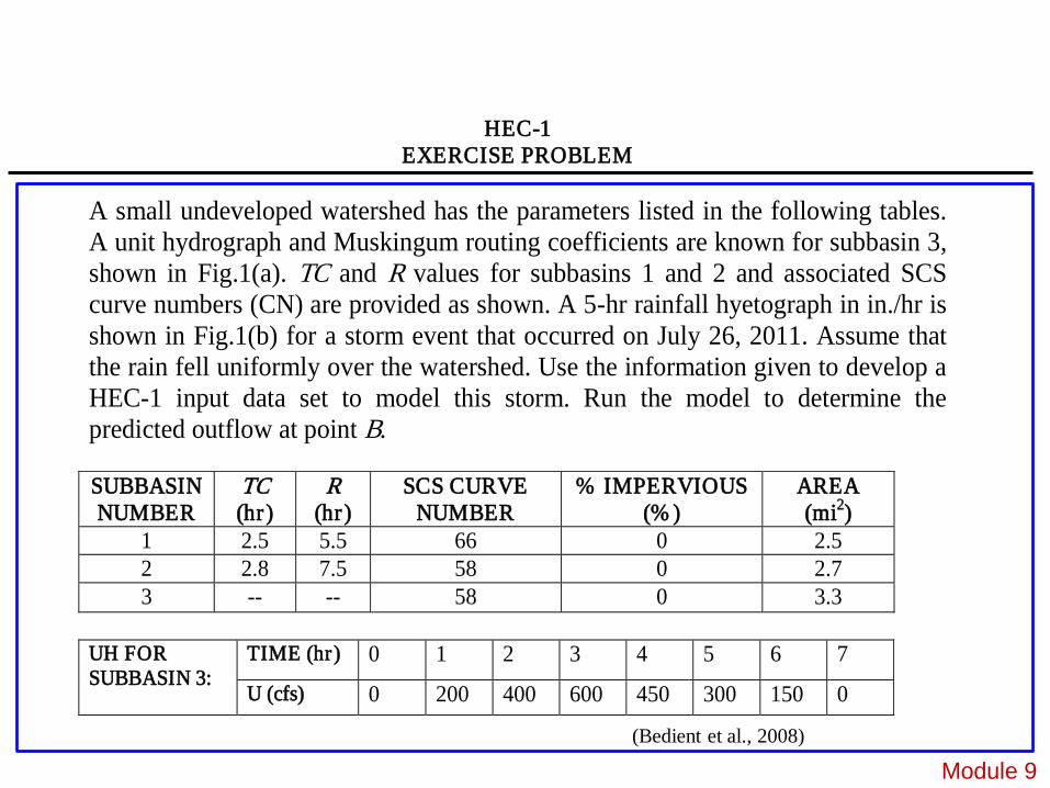
A small undeveloped watershed has the parameters listed in the following tables. A unit hydrograph and Muskingum routing coefficients are known for subbasin 3, shown in Fig.1(a). TC and R values for subbasins 1 and 2 and associated SCS curve numbers (CN) are provided as shown. A 5-hr rainfall hyetograph in in./hr is shown in Fig.1(b) for a storm event that occurred on July 26, 2011. Assume that the rain fell uniformly over the watershed. Use the information given to develop a HEC-1 input data set to model this storm. Run the model to determine the predicted outflow at point B. SUBBASIN NUMBER

TC (hr)

R (hr )

SCS CURVE NUMBER

% IMPERVIOUS (% )

AREA (mi2)

1 2.5 5.5 66 0 2.5 2 2.8 7.5 58 0 2.7 3 -- -- 58 0 3.3

UH FOR SUBBASIN 3:

TIME (hr) 0 1 2 3 4 5 6 7

U (cfs) 0 200 400 600 450 300 150 0

(Bedient et al., 2008)

Module 9

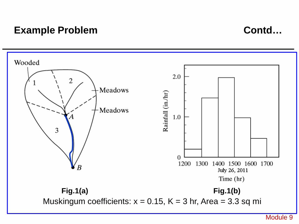
Fig.1(a) Fig.1(b)Muskingum coefficients: x = 0.15, K = 3 hr, Area = 3.3 sq mi

Module 9

Example Problem Contd…

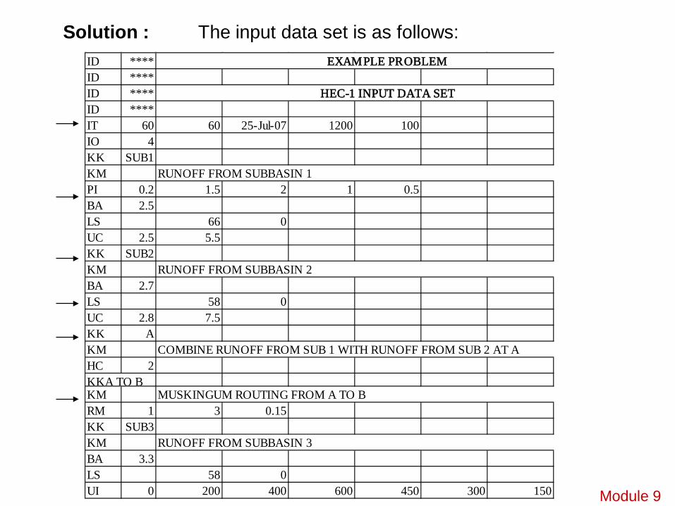
ID ****ID ****ID ****ID ****IT 60 60 25-Jul-07 1200 100IO 4KK SUB1KMPI 0.2 1.5 2 1 0.5BA 2.5LS 66 0UC 2.5 5.5KK SUB2KMBA 2.7LS 58 0UC 2.8 7.5KK AKMHC 2

KMRM 1 3 0.15KK SUB3KMBA 3.3LS 58 0UI 0 200 400 600 450 300 150

MUSKINGUM ROUTING FROM A TO B

RUNOFF FROM SUBBASIN 3

KKA TO B

EXAMPLE PROBLEM

HEC-1 INPUT DATA SET



COMBINE RUNOFF FROM SUB 1 WITH RUNOFF FROM SUB 2 AT A

Solution : The input data set is as follows:

Module 9

Using HEC-HMS Contd…

Three components

Basin model - contains the elements of the basin, their connectivity, and

runoff parameters ( It will be discussed in detail later)

Meteorologic Model - contains the rainfall and evapotranspiration data

Control Specifications - contains the start/stop timing and calculation

intervals for the run

Module 9

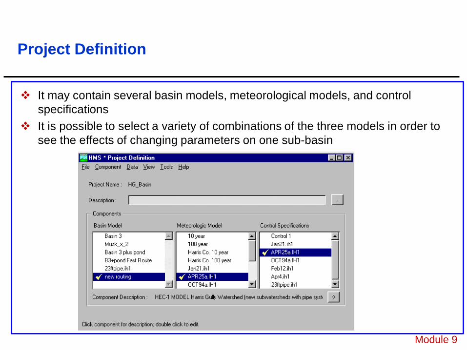
Project Definition

It may contain several basin models, meteorological models, and control specifications

It is possible to select a variety of combinations of the three models in order to see the effects of changing parameters on one sub-basin

Module 9

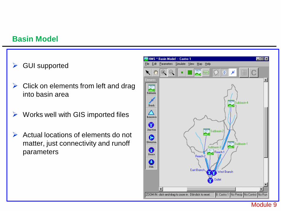
Basin Model

GUI supported

Click on elements from left and drag into basin area

Works well with GIS imported files

Actual locations of elements do not matter, just connectivity and runoff parameters

Module 9

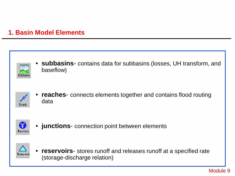
1. Basin Model Elements

• subbasins- contains data for subbasins (losses, UH transform, and baseflow)

• reaches- connects elements together and contains flood routing data

• junctions- connection point between elements

• reservoirs- stores runoff and releases runoff at a specified rate (storage-discharge relation)

Module 9

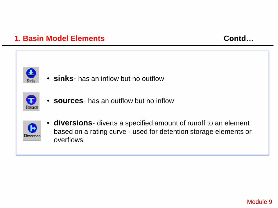
1. Basin Model Elements Contd…

• sinks- has an inflow but no outflow

• sources- has an outflow but no inflow

• diversions- diverts a specified amount of runoff to an element based on a rating curve - used for detention storage elements or overflows

Module 9

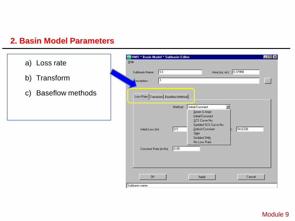
a) Loss rate

b) Transform

c) Baseflow methods

Module 9

2. Basin Model Parameters

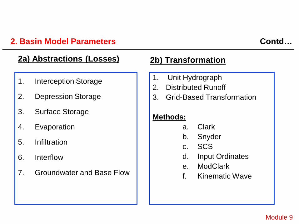
2a) Abstractions (Losses)

1. Interception Storage

2. Depression Storage

3. Surface Storage

4. Evaporation

5. Infiltration

6. Interflow

7. Groundwater and Base Flow

Module 9

2. Basin Model Parameters Contd…

1. Unit Hydrograph2. Distributed Runoff3. Grid-Based Transformation

Methods:a. Clark b. Snyder c. SCSd. Input Ordinates e. ModClarkf. Kinematic Wave

2b) Transformation

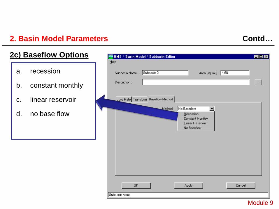
2c) Baseflow Options

a. recession

b. constant monthly

c. linear reservoir

d. no base flow

Module 9

2. Basin Model Parameters Contd…

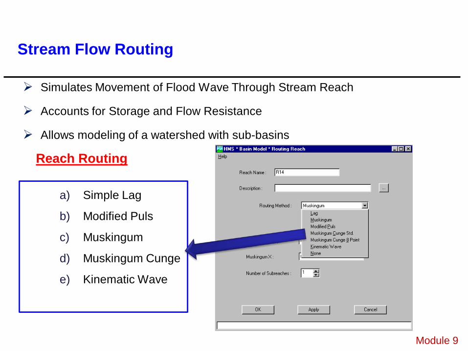
Stream Flow Routing

Simulates Movement of Flood Wave Through Stream Reach

Accounts for Storage and Flow Resistance

Allows modeling of a watershed with sub-basins

Module 9

a) Simple Lag

b) Modified Puls

c) Muskingum

d) Muskingum Cunge

e) Kinematic Wave

Reach Routing

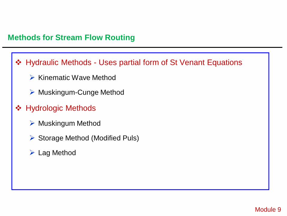
Hydraulic Methods - Uses partial form of St Venant Equations

Kinematic Wave Method

Muskingum-Cunge Method

Hydrologic Methods

Muskingum Method

Storage Method (Modified Puls)

Lag Method

Module 9

Methods for Stream Flow Routing

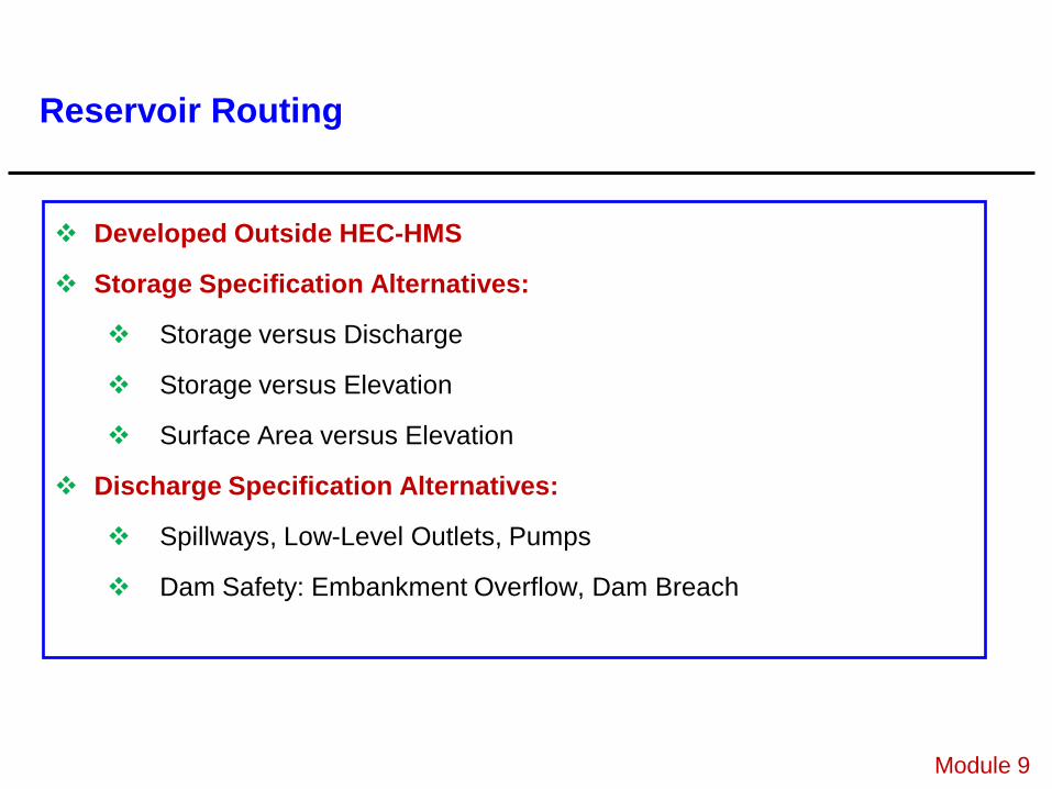
Developed Outside HEC-HMS

Storage Specification Alternatives:

Storage versus Discharge

Storage versus Elevation

Surface Area versus Elevation

Discharge Specification Alternatives:

Spillways, Low-Level Outlets, Pumps

Dam Safety: Embankment Overflow, Dam Breach

Module 9

Reservoir Routing

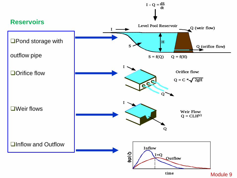
Reservoirs

Q (cfs)

I=Q

time

Q (cfs)

Inflow

Outflow

I - Q = dS dt

Level Pool Reservoir Q (weir flow)

Q (orifice flow)

I

SH

S = f(Q) Q = f(H)

Orifice flow:

Q = C * 2gH

Q

I

I

Weir Flow: Q = CLH3/2

Q

Pond storage with

outflow pipe

Orifice flow

Weir flows

Inflow and Outflow

Module 9

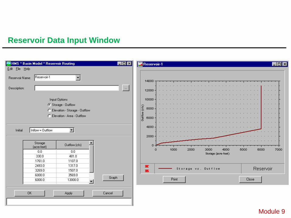
Initial Conditions to be considered

Inflow = Outflow

Initial Storage Values

Initial Outflow

Initial Elevation

Elevation Data relates to both Storage/Area and Discharge

HEC-1 Routing routines with initial conditions and elevation data

can be imported as Reservoir Elements

Module 9

Reservoir Data Input

Module 9

Reservoir Data Input Window

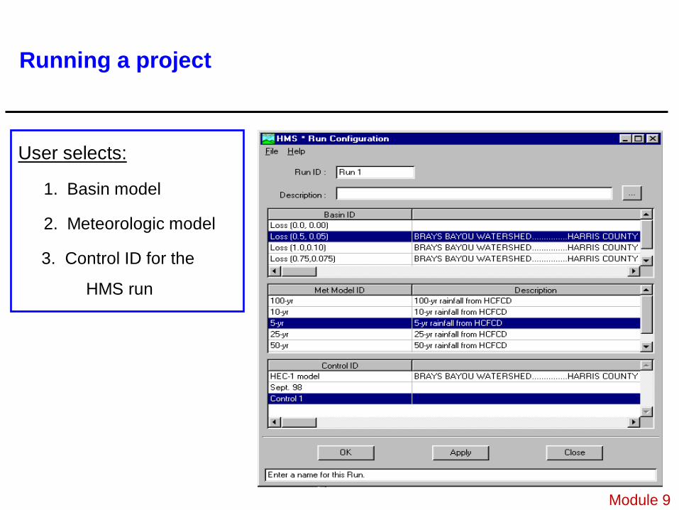
User selects:

1. Basin model

2. Meteorologic model

3. Control ID for the

HMS run

Running a project

Module 9

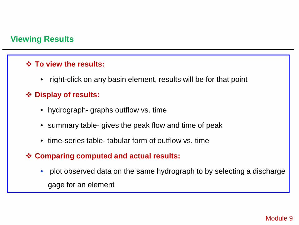
To view the results:

• right-click on any basin element, results will be for that point

Display of results:

• hydrograph- graphs outflow vs. time

• summary table- gives the peak flow and time of peak

• time-series table- tabular form of outflow vs. time

Comparing computed and actual results:

• plot observed data on the same hydrograph to by selecting a discharge

gage for an element

Module 9

Viewing Results

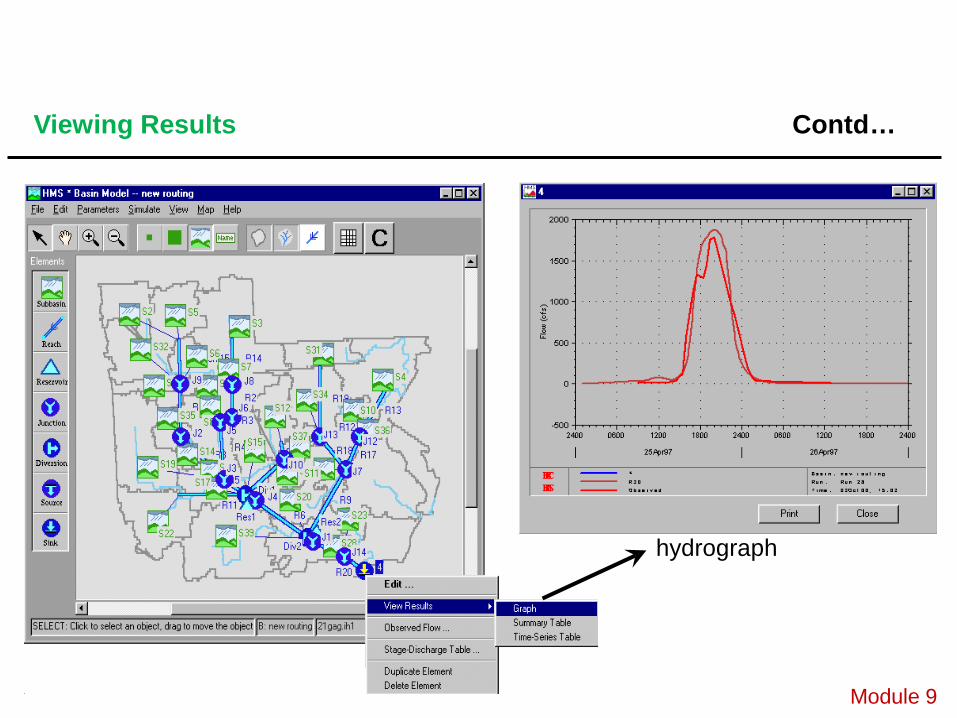
hydrograph

Module 9

Viewing Results Contd…

HEC-HMS Output

1. Tables

Summary

Detailed (Time Series)

2. Hyetograph Plots

3. Sub-Basin Hydrograph Plots

4. Routed Hydrograph Plots

5. Combined Hydrograph Plots

6. Recorded Hydrographs - comparison

Module 9

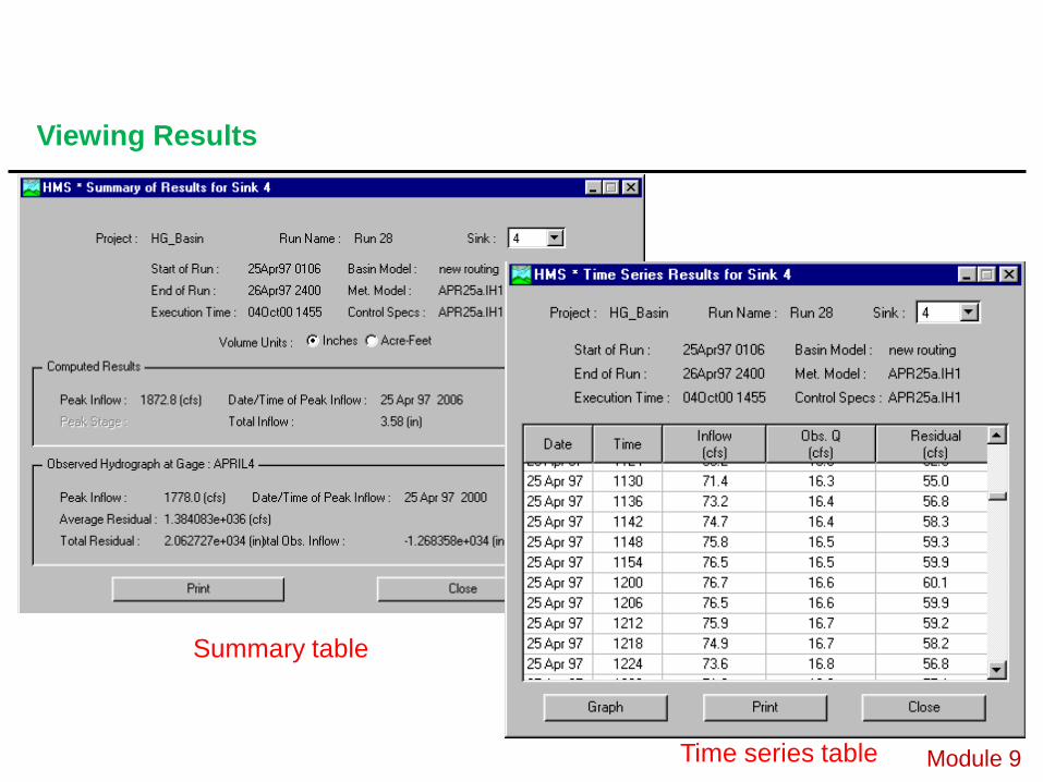
Summary table

Time series table Module 9

Viewing Results

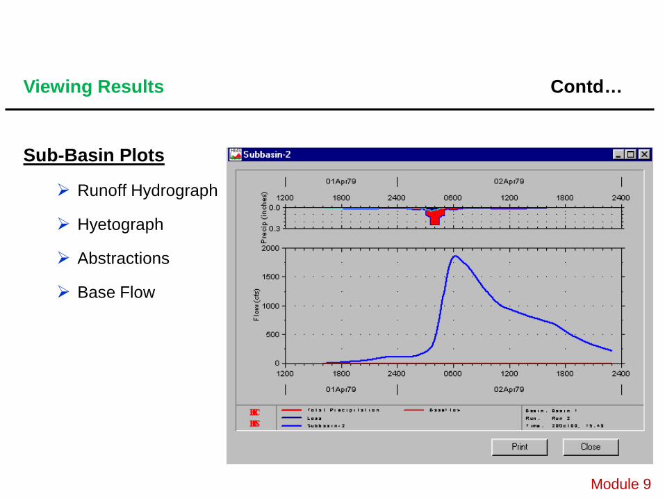
Sub-Basin Plots

Runoff Hydrograph

Hyetograph

Abstractions

Base Flow

Module 9


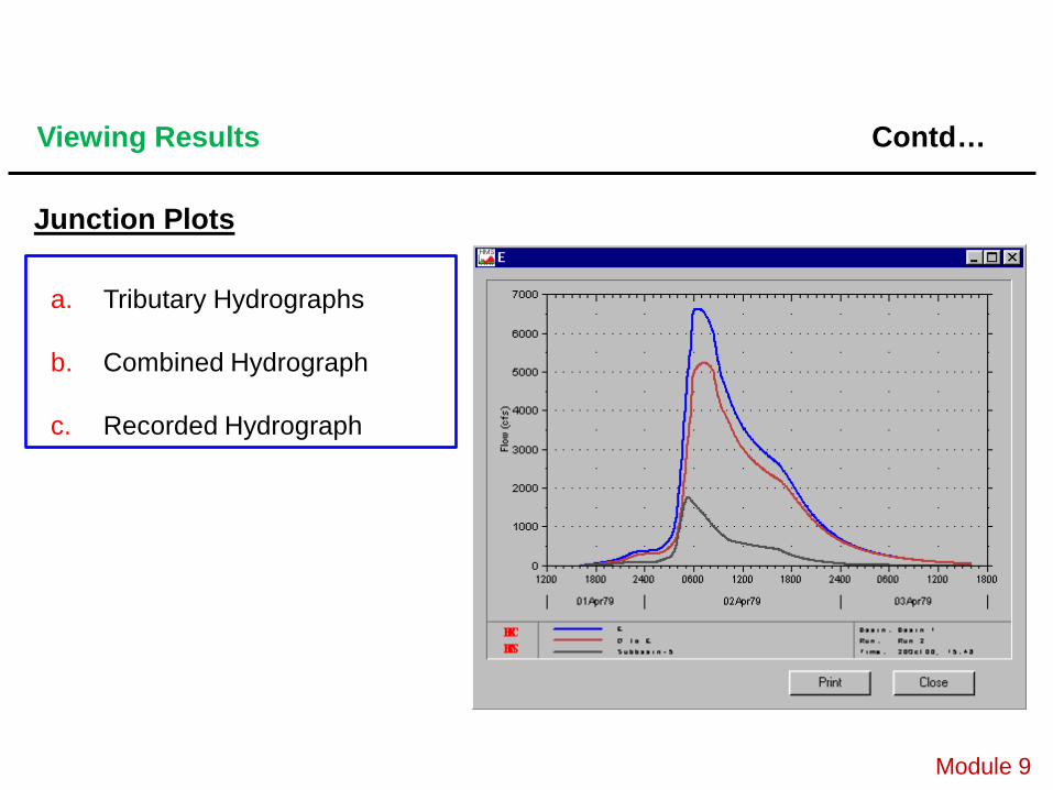
Junction Plots

Module 9

a. Tributary Hydrographs

b. Combined Hydrograph

c. Recorded Hydrograph


Documents

Lecture 3: Major hydrologic models-HSPF, HEC and MIKE · HEC-HMS Background. Purpose of HEC -HMS Improved User Interface, Graphics, and Reporting Improved Hydrologic Computations