Lecture 5:Causality and

Feature Selection

Isabelle Guyonisabelle@clopinet.com

Variable/feature selection

Remove features Xi to improve (or least degrade) prediction of Y.

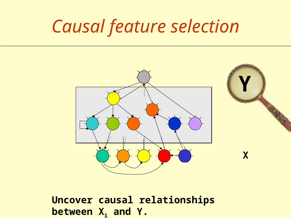
X

Y

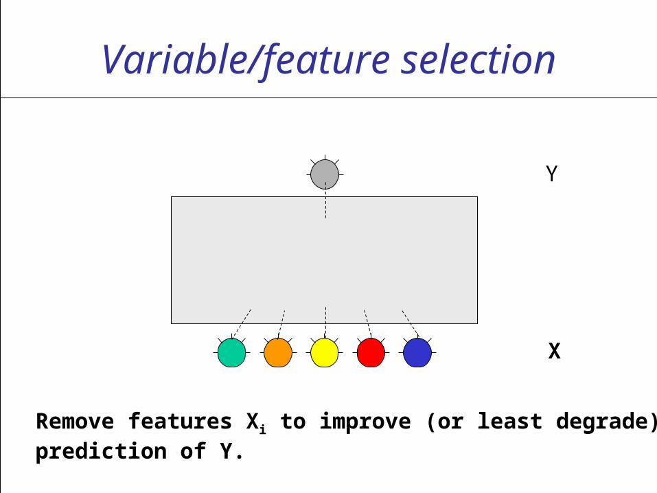
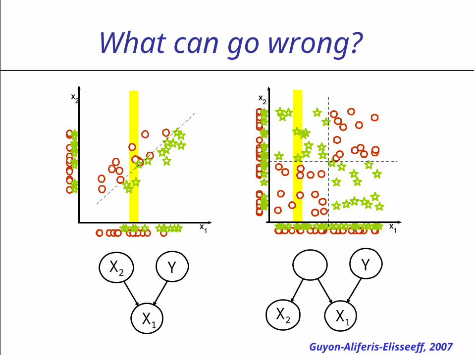
What can go wrong?

Guyon-Aliferis-Elisseeff, 2007

X2 X1

180 190 200 210 220 230 240 250 260

20

40

60

80

100

120

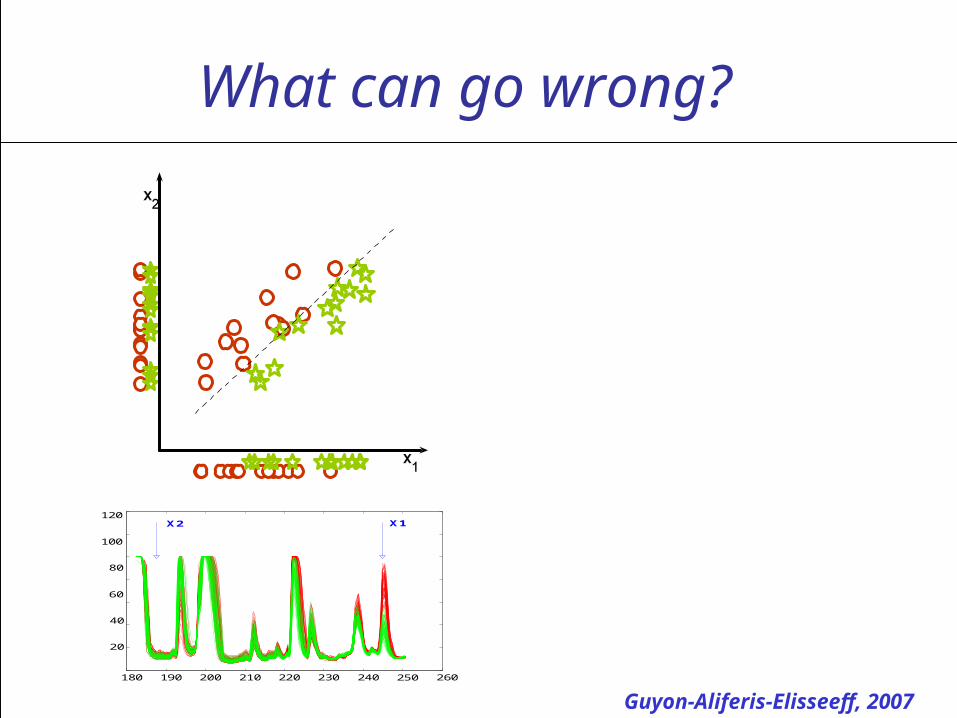
What can go wrong?

20 40 60 80 100

8

10

12

14

16

20

40

60

80

100

X2 X1

X1

X

2

X2 X1

180 190 200 210 220 230 240 250 260

20

40

60

80

100

120

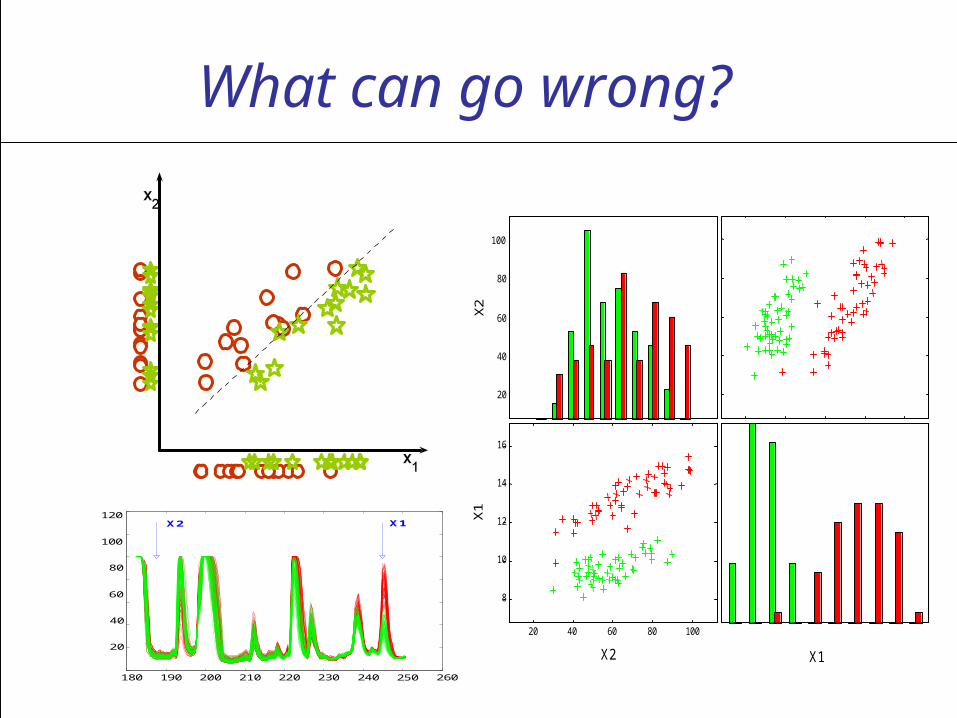
What can go wrong?

Guyon-Aliferis-Elisseeff, 2007

X2 Y

X1

Y

X1X2

X

Y

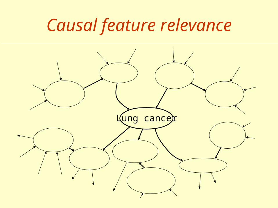
Causal feature selection

Uncover causal relationships between Xi and Y.

Y

Lung cancer

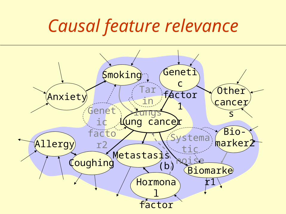
Causal feature relevance

Lung cancer

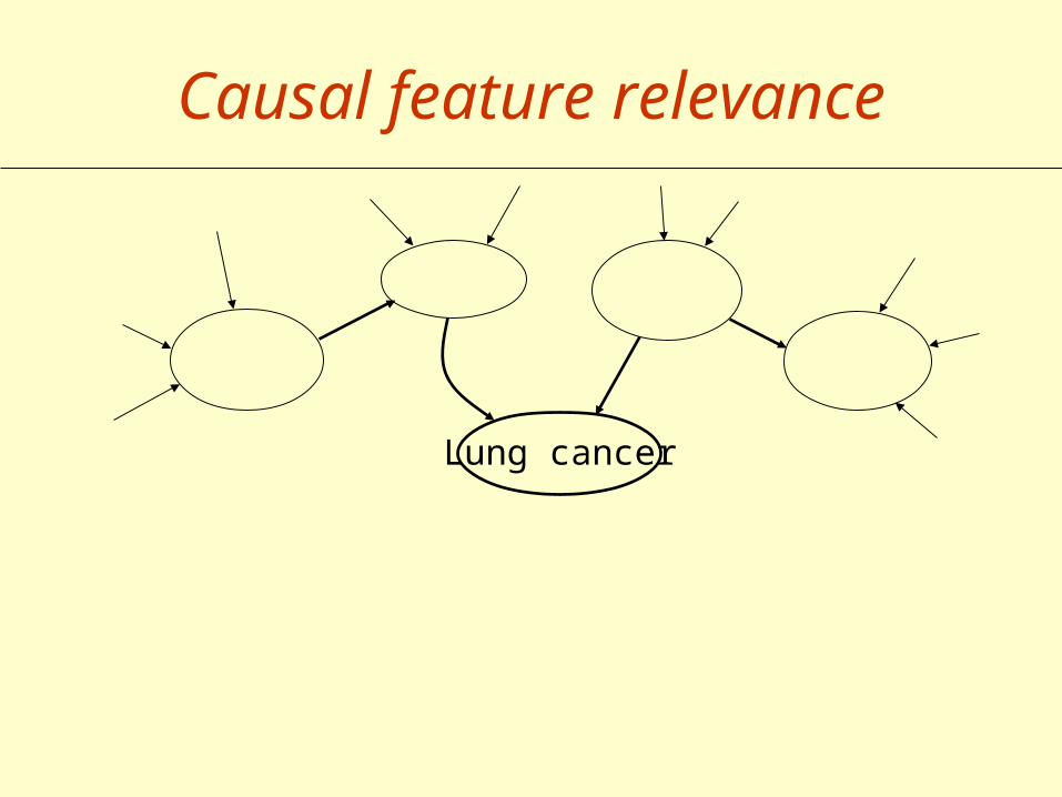
Causal feature relevance

Lung cancer

Causal feature relevance

Lung cancer

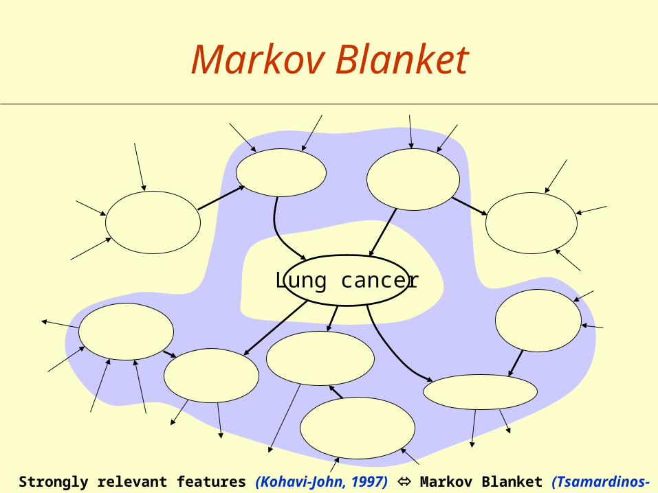
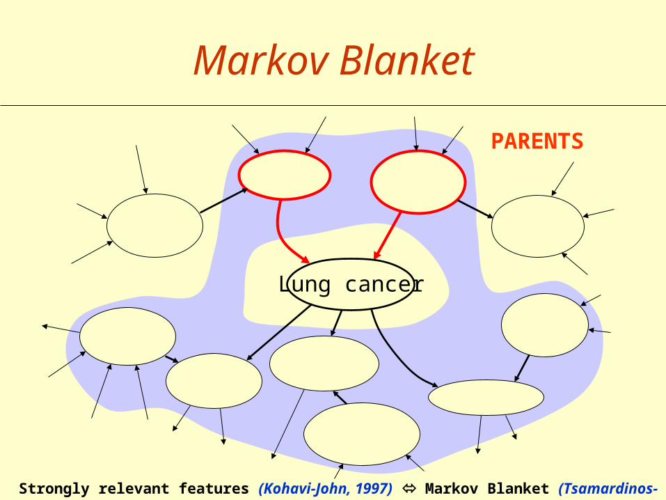
Markov Blanket

Strongly relevant features (Kohavi-John, 1997) Markov Blanket (Tsamardinos-Aliferis, 2003)

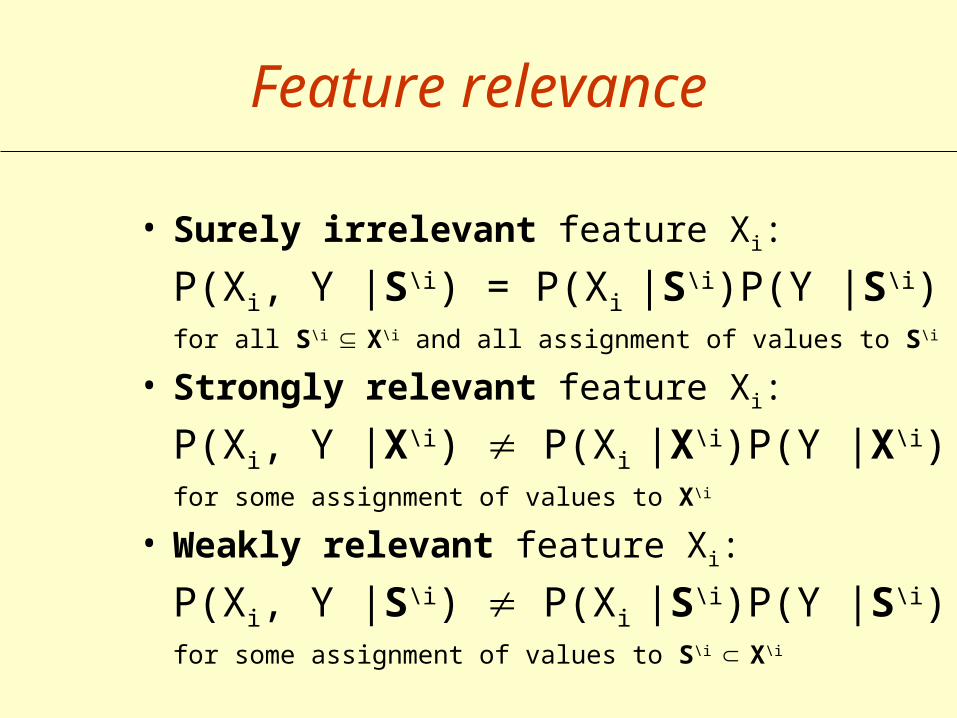
Feature relevance

• Surely irrelevant feature Xi:

P(Xi, Y |S\i) = P(Xi |S\i)P(Y |S\i)for all S\i X\i and all assignment of values to S\i

• Strongly relevant feature Xi:

P(Xi, Y |X\i) P(Xi |X\i)P(Y |X\i)for some assignment of values to X\i

• Weakly relevant feature Xi:

P(Xi, Y |S\i) P(Xi |S\i)P(Y |S\i)for some assignment of values to S\i X\i

Lung cancer

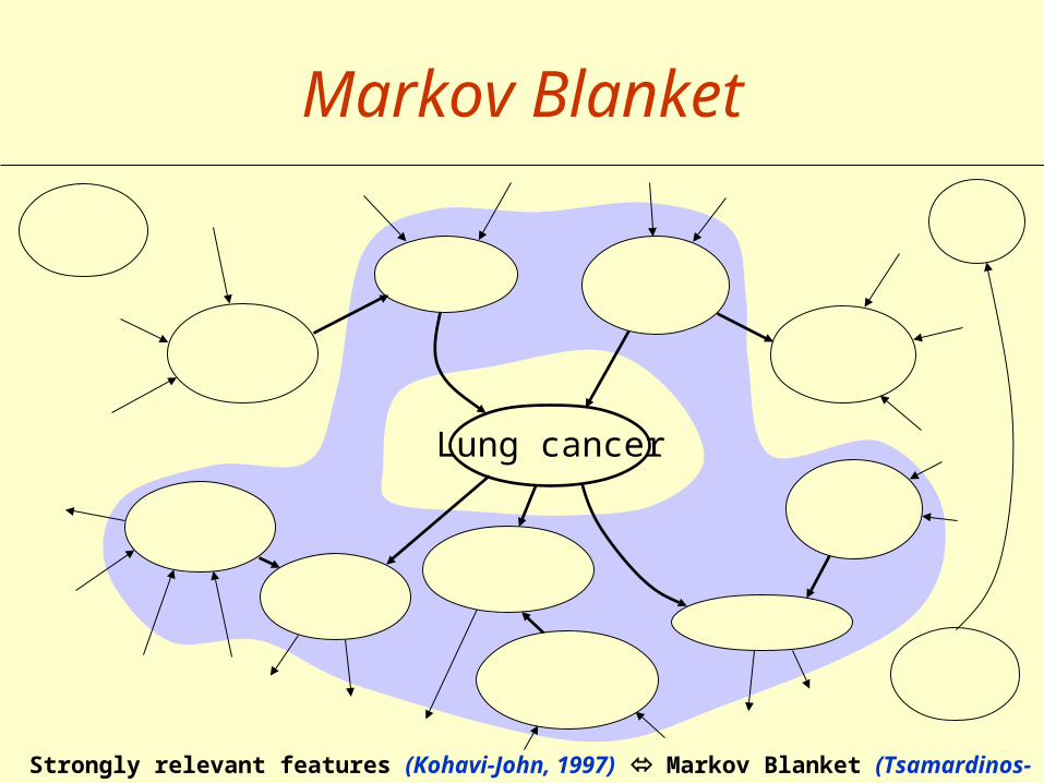
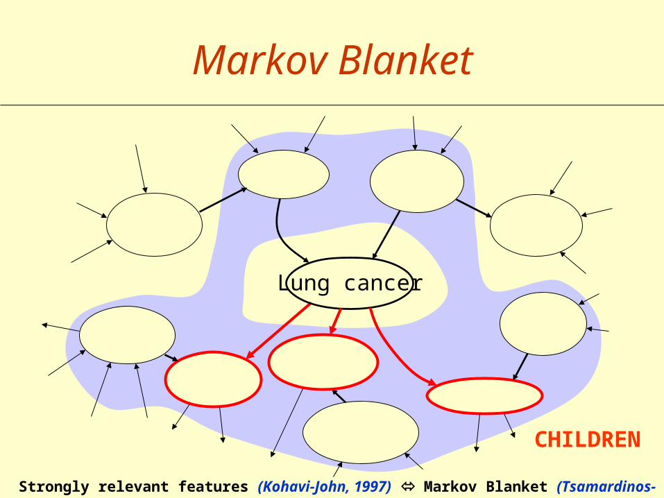
Markov Blanket

Strongly relevant features (Kohavi-John, 1997) Markov Blanket (Tsamardinos-Aliferis, 2003)

Lung cancer

Strongly relevant features (Kohavi-John, 1997) Markov Blanket (Tsamardinos-Aliferis, 2003)

PARENTS

Markov Blanket

Lung cancer

Strongly relevant features (Kohavi-John, 1997) Markov Blanket (Tsamardinos-Aliferis, 2003)

CHILDREN

Markov Blanket

Lung cancer

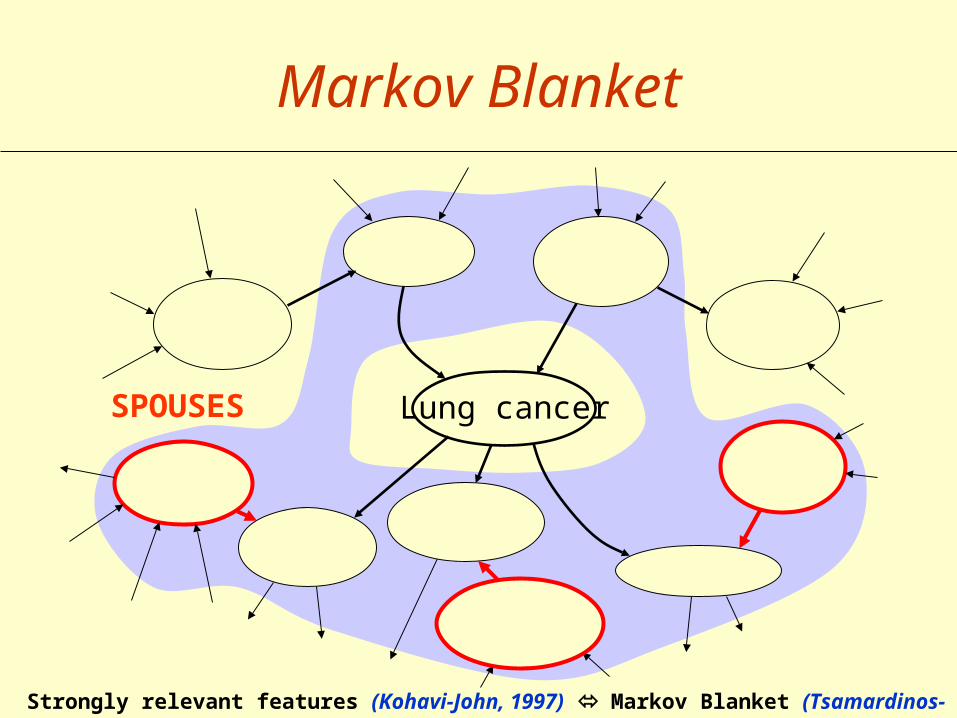
Strongly relevant features (Kohavi-John, 1997) Markov Blanket (Tsamardinos-Aliferis, 2003)

SPOUSES

Markov Blanket

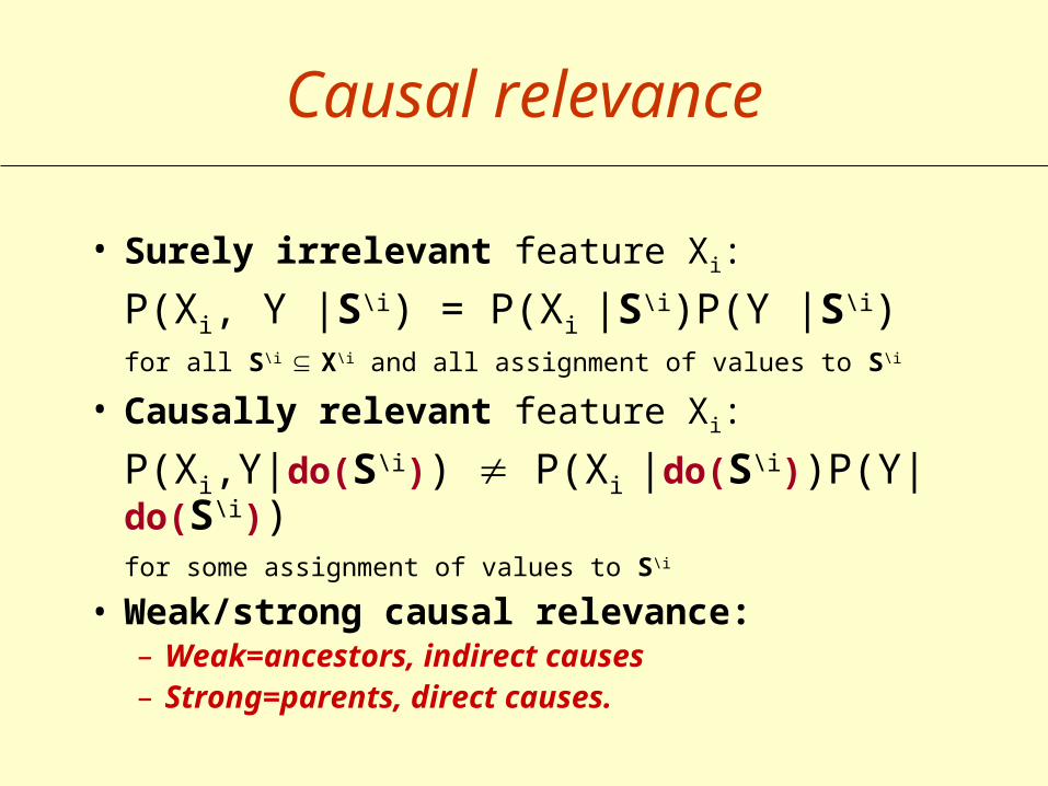
Causal relevance

• Surely irrelevant feature Xi:

P(Xi, Y |S\i) = P(Xi |S\i)P(Y |S\i)for all S\i X\i and all assignment of values to S\i

• Causally relevant feature Xi:

P(Xi,Y|do(S\i)) P(Xi |do(S\i))P(Y|do(S\i))for some assignment of values to S\i

• Weak/strong causal relevance: – Weak=ancestors, indirect causes– Strong=parents, direct causes.

Lung cancer

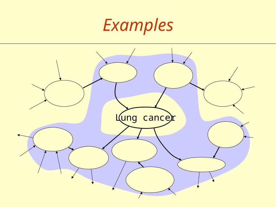
Examples

Smoking

Lung cancer

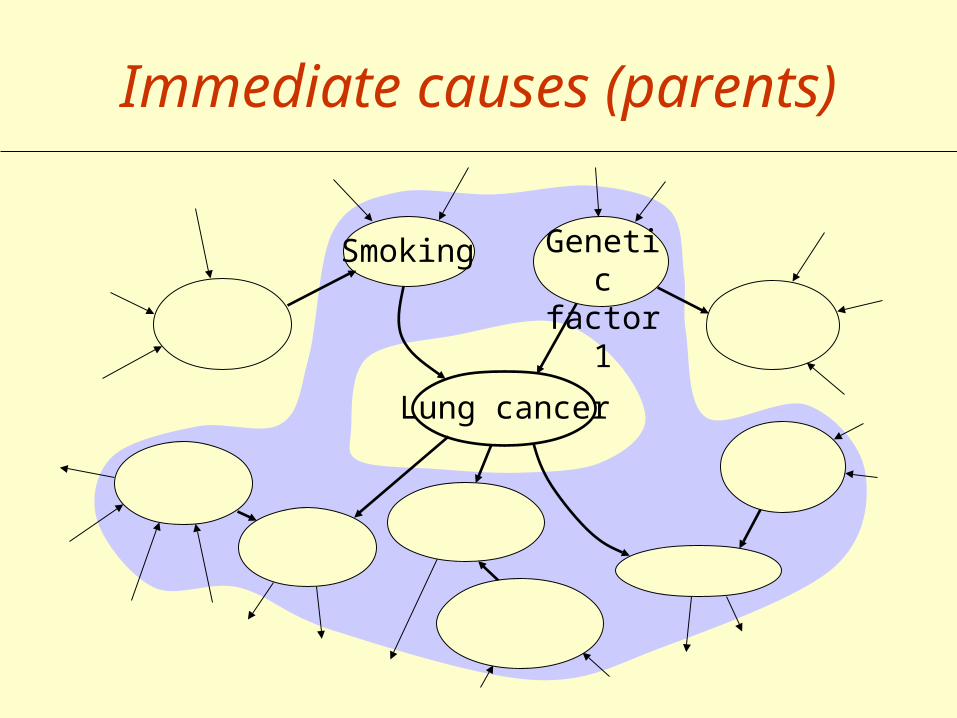
Immediate causes (parents)

Genetic factor1

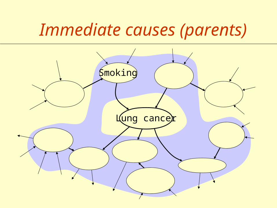
Smoking

Lung cancer

Immediate causes (parents)

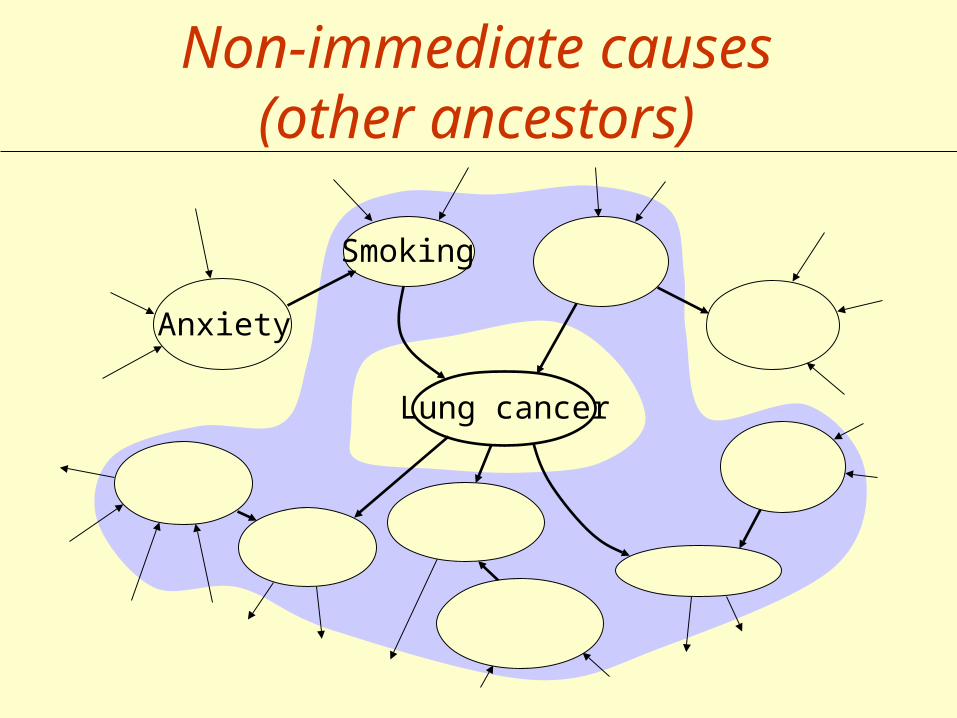
Smoking

Anxiety

Lung cancer

Non-immediate causes (other ancestors)

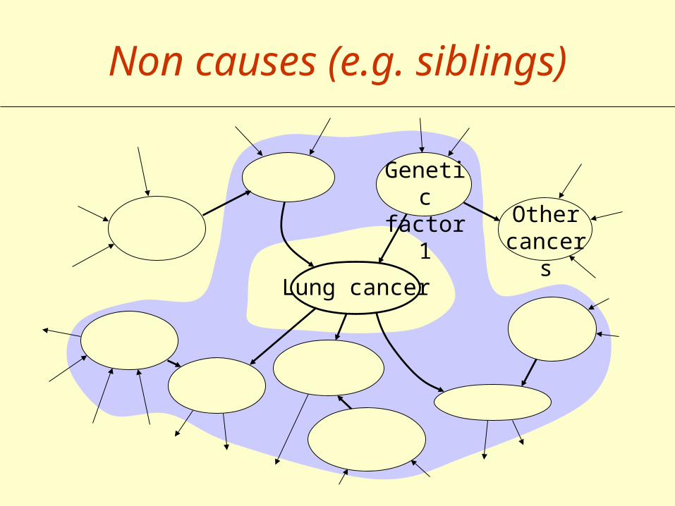
Genetic factor1

Other cancers

Lung cancer

Non causes (e.g. siblings)

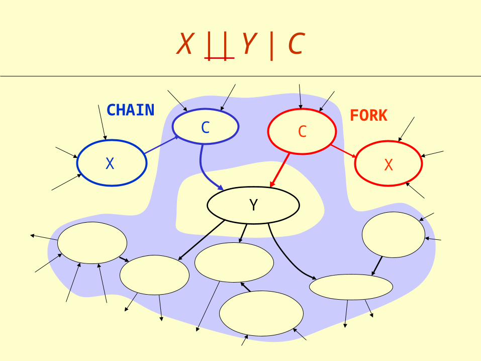
Y

X || Y | C

FORKCHAIN

X X

C C

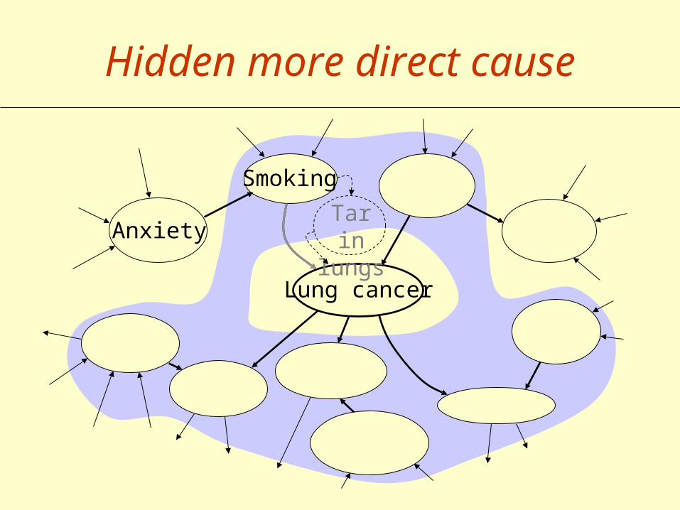
Smoking

Anxiety

Lung cancer

Hidden more direct cause

Tar in lungs

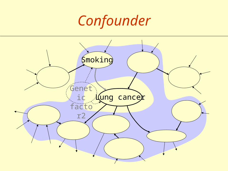
Smoking

Lung cancer

Confounder

Genetic factor2

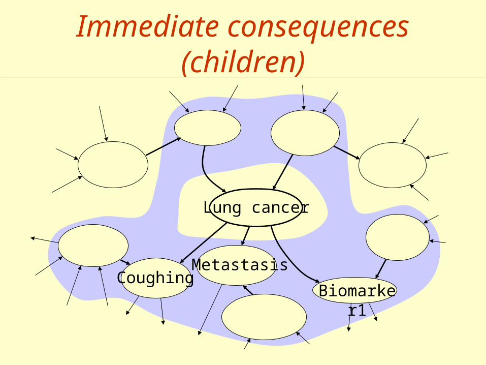
Coughing Metastasis

Lung cancer

Biomarker1

Immediate consequences (children)

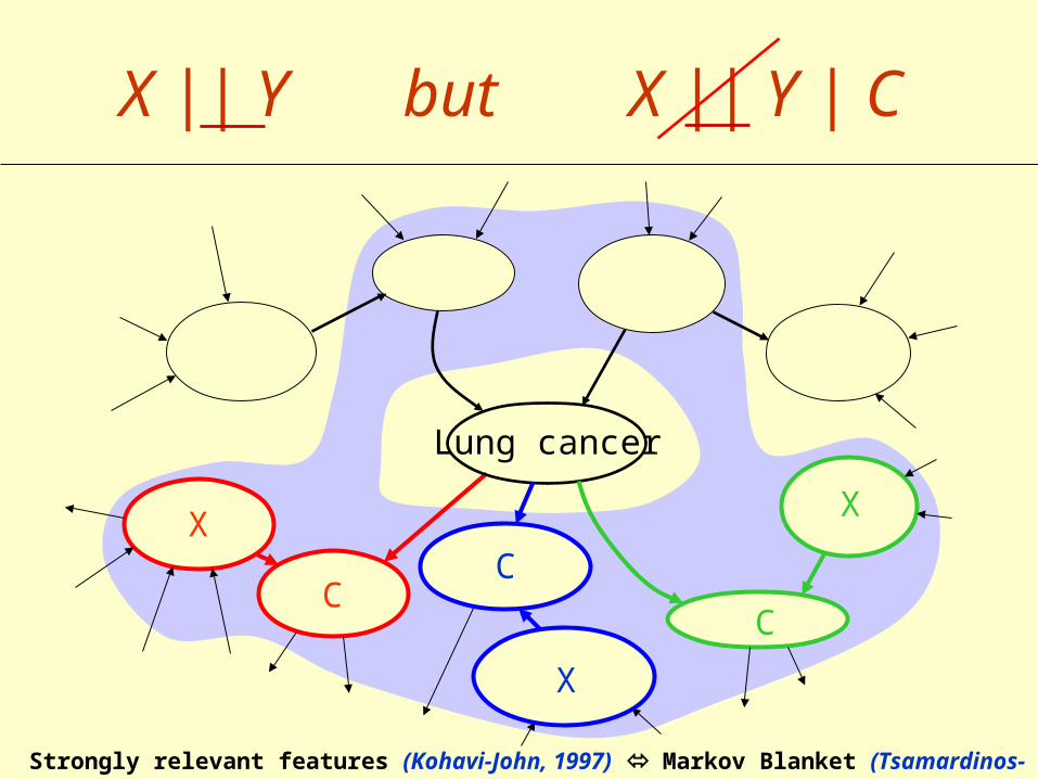
Lung cancer

Strongly relevant features (Kohavi-John, 1997) Markov Blanket (Tsamardinos-Aliferis, 2003)

X

C

X

C

X

C

X || Y but X || Y | C

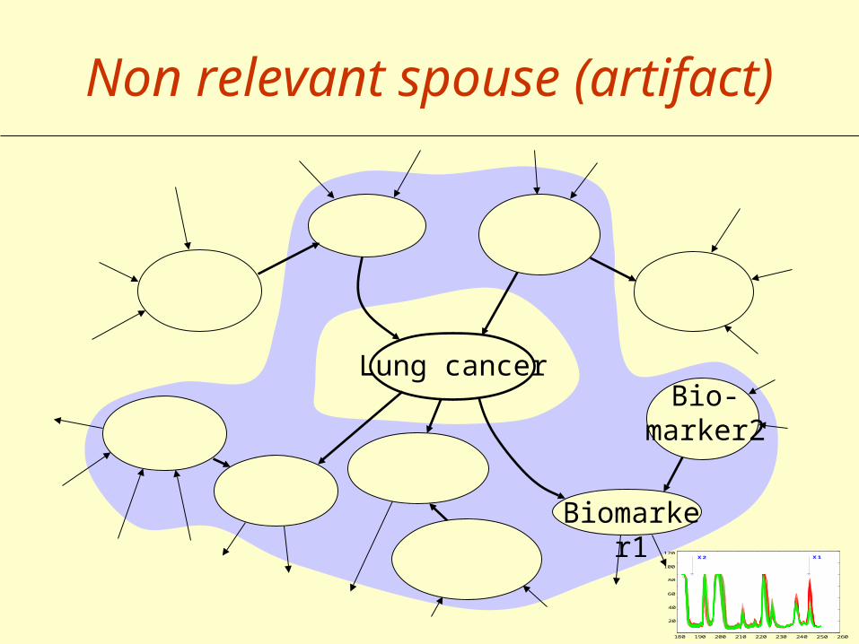
Lung cancerBio-

marker2

Biomarker1

Non relevant spouse (artifact)

X2 X1

180 190 200 210 220 230 240 250 260

20

40

60

80

100

120

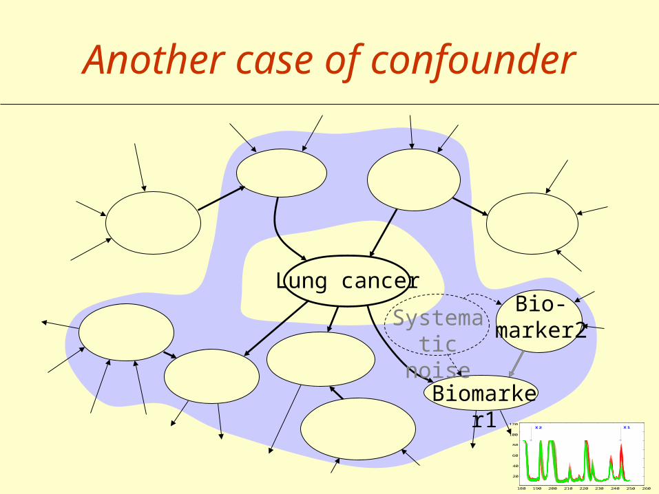
Lung cancerBio-

marker2

Biomarker1

Another case of confounder

X2 X1

180 190 200 210 220 230 240 250 260

20

40

60

80

100

120

Systematic noise

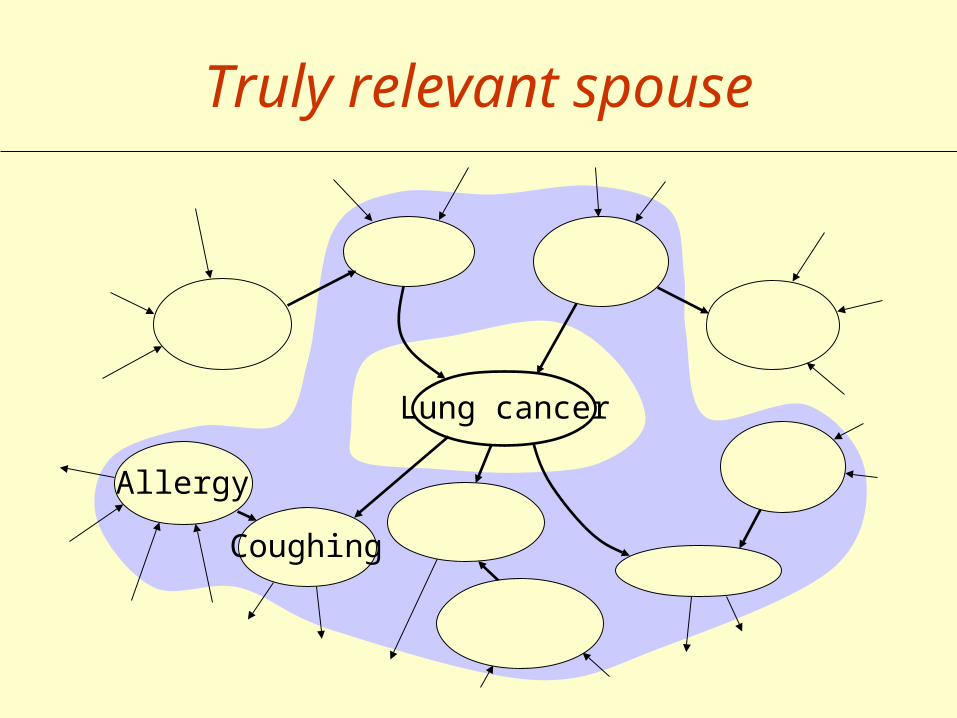
Coughing

Allergy

Lung cancer

Truly relevant spouse

Hormonal factor

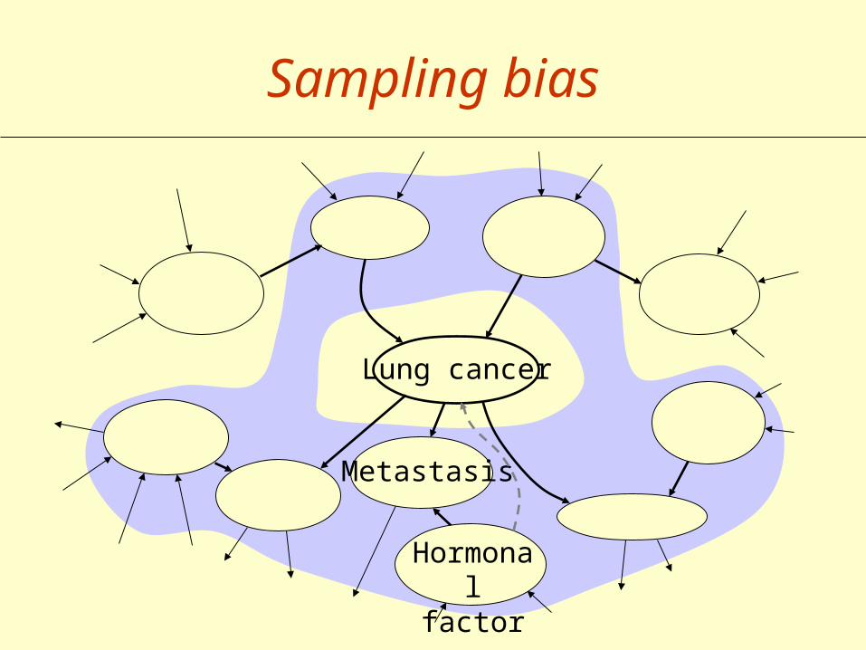
Metastasis

Lung cancer

Sampling bias

Coughing

Allergy

Smoking

Anxiety

Genetic factor1

Hormonal factor

Metastasis(b)

Other cancers

Lung cancerGenetic factor2

Tar in lungs

Bio-marker2

Biomarker1

Systematic noise

Causal feature relevance

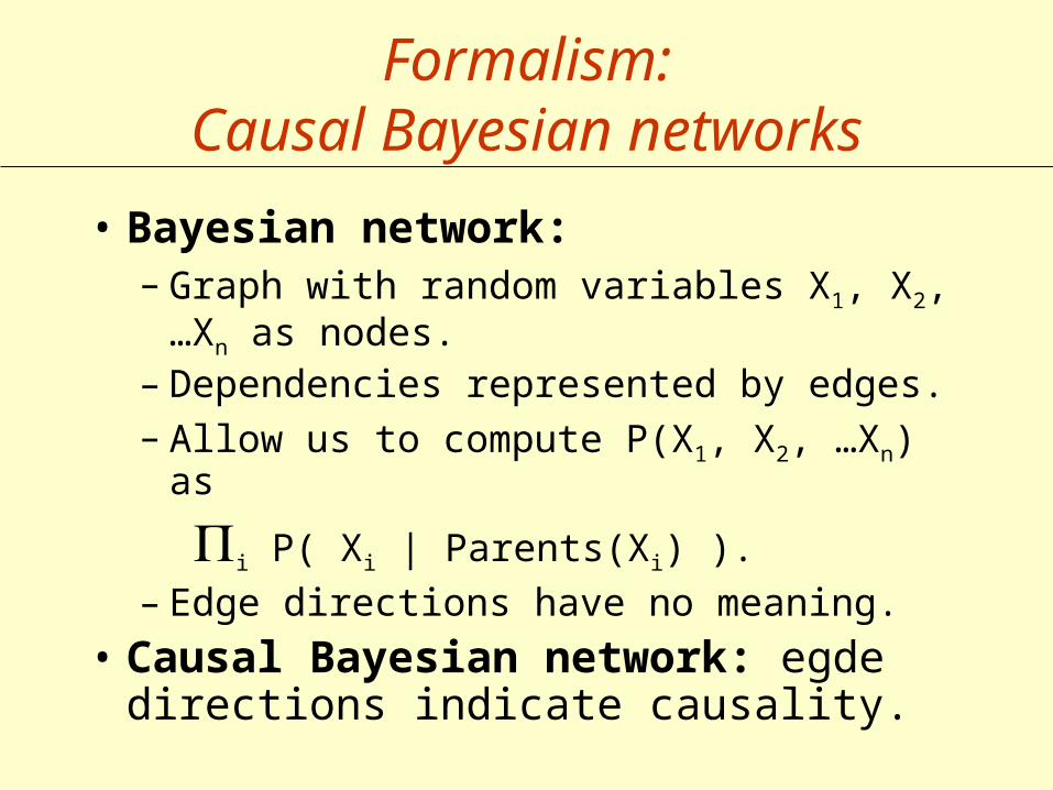
Formalism:Causal Bayesian networks

• Bayesian network:– Graph with random variables X1, X2, …Xn as

nodes.– Dependencies represented by edges.– Allow us to compute P(X1, X2, …Xn) as

i P( Xi | Parents(Xi) ).

– Edge directions have no meaning.

• Causal Bayesian network: egde directions indicate causality.

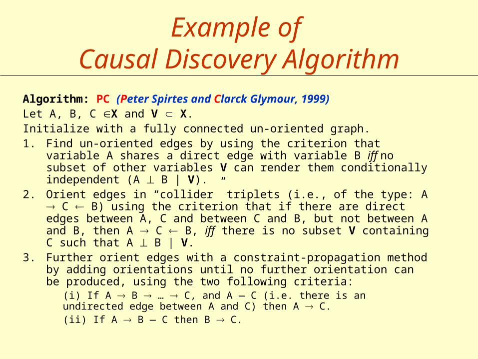
Example of Causal Discovery Algorithm

Algorithm: PC (Peter Spirtes and Clarck Glymour, 1999)Let A, B, C X and V X. Initialize with a fully connected un-oriented graph.1. Find un-oriented edges by using the criterion that variable A

shares a direct edge with variable B iff no subset of other variables V can render them conditionally independent (A B | V).

2. Orient edges in “collider” triplets (i.e., of the type: A C B) using the criterion that if there are direct edges between A, C and between C and B, but not between A and B, then A C B, iff there is no subset V containing C such that A B | V.

3. Further orient edges with a constraint-propagation method by adding orientations until no further orientation can be produced, using the two following criteria:

(i) If A B … C, and A — C (i.e. there is an undirected edge between A and C) then A C. (ii) If A B — C then B C.

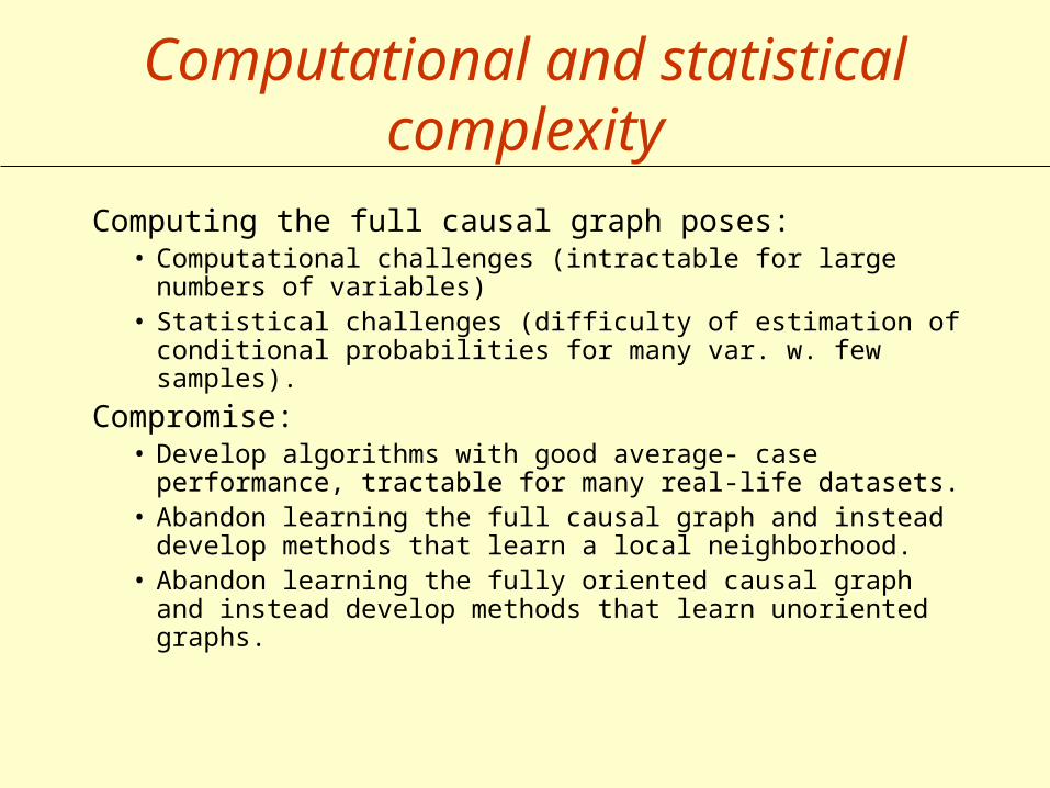
Computational and statistical complexity

Computing the full causal graph poses:• Computational challenges (intractable for large numbers of

variables)• Statistical challenges (difficulty of estimation of conditional

probabilities for many var. w. few samples).

Compromise:• Develop algorithms with good average- case

performance, tractable for many real-life datasets.• Abandon learning the full causal graph and instead

develop methods that learn a local neighborhood.• Abandon learning the fully oriented causal graph and

instead develop methods that learn unoriented graphs.

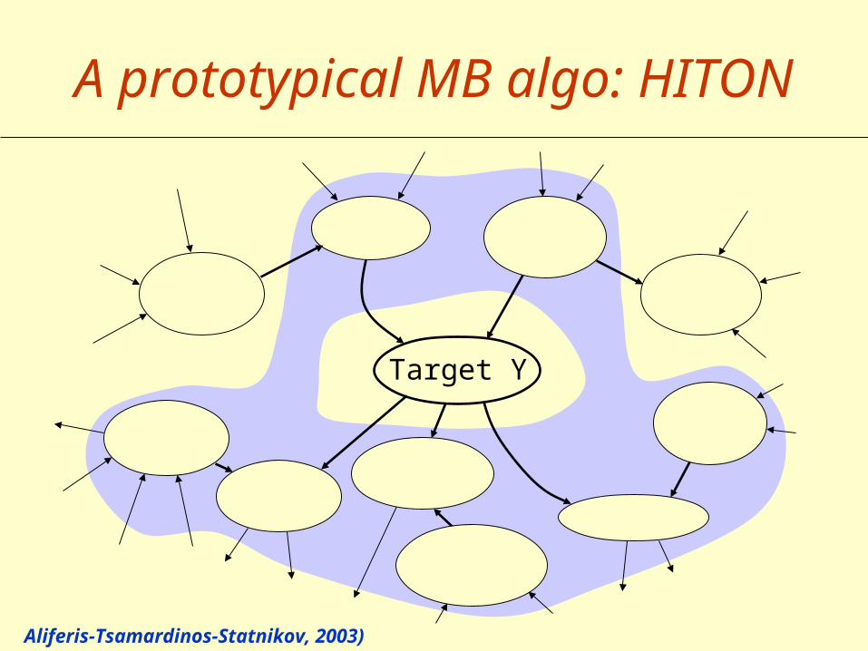
Target Y

A prototypical MB algo: HITON

Aliferis-Tsamardinos-Statnikov, 2003)

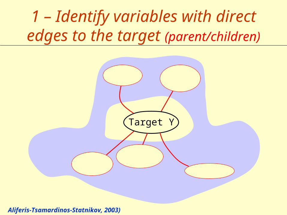
Target Y

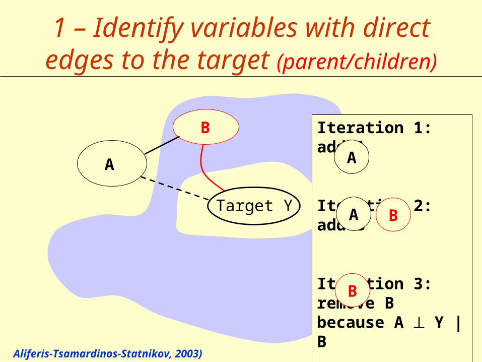
1 – Identify variables with direct edges to the target

(parent/children)

Aliferis-Tsamardinos-Statnikov, 2003)

Target Y

Aliferis-Tsamardinos-Statnikov, 2003)

1 – Identify variables with direct edges to the target

(parent/children)

A

B Iteration 1: add A

Iteration 2: add B

Iteration 3: remove B because A Y | B

etc.

A

A B

B

Target Y

Aliferis-Tsamardinos-Statnikov, 2003)

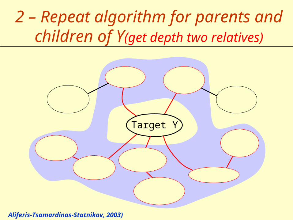
2 – Repeat algorithm for parents and children of Y(get

depth two relatives)

Target Y

Aliferis-Tsamardinos-Statnikov, 2003)

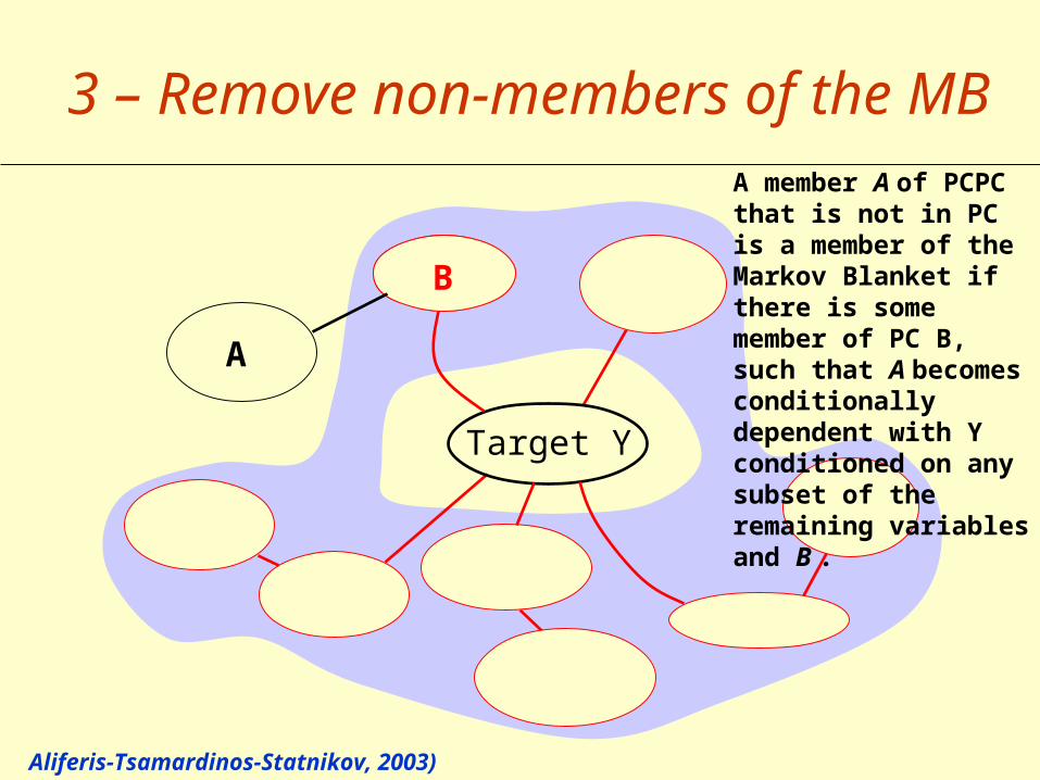
3 – Remove non-members of the MB

A member A of PCPC that is not in PC is a member of the Markov Blanket if there is some member of PC B, such that A becomes conditionally dependent with Y conditioned on any subset of the remaining variables and B .

A

B

Conclusion

• Feature selection focuses on uncovering subsets of variables X1, X2, … predictive of the target Y.

• Multivariate feature selection is in principle more powerful than univariate feature selection, but not always in practice.

• Taking a closer look at the type of dependencies in terms of causal relationships may help refining the notion of variable relevance.

1) Feature Extraction, Foundations and ApplicationsI. Guyon et al, Eds.Springer, 2006.http://clopinet.com/fextract-book

2) Causal feature selectionI. Guyon, C. Aliferis, A. ElisseeffTo appear in “Computational Methods of Feature Selection”, Huan Liu and Hiroshi Motoda Eds., Chapman and Hall/CRC Press, 2007.http://clopinet.com/isabelle/Papers/causalFS.pdf

Acknowledgements and references