Embed Size (px)
Citation preview
Chemical Engineering 160/260Polymer Science and Engineering
Lecture 5 - Indirect Measures ofLecture 5 - Indirect Measures ofMolecular Weight: Intrinsic ViscosityMolecular Weight: Intrinsic Viscosityand Gel Permeation Chromatographyand Gel Permeation Chromatography
January 26, 2001January 26, 2001
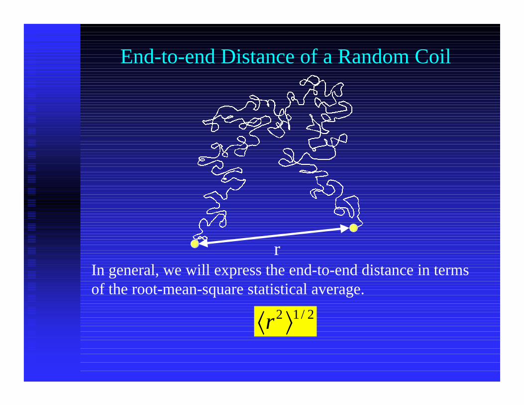
End-to-end Distance of a Random Coil
rIn general, we will express the end-to-end distance in termsof the root-mean-square statistical average.
⟨ ⟩r2 1 2/
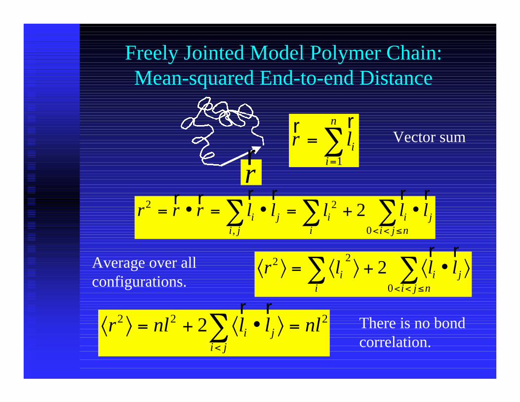
Freely Jointed Model Polymer Chain:Mean-squared End-to-end Distance
r rr li
i
n
==∑
1
r r r l l l l li j
i ji
ii j
i j n
2 2
0
2= • = • = + •∑ ∑ ∑< < ≤
r r r r r r
,
⟨ ⟩ = ⟨ ⟩ + ⟨ • ⟩∑ ∑
< < ≤
r l l lii
ii j n
j2 2
0
2r r
⟨ ⟩ = + ⟨ • ⟩ =
<∑r nl l l nlii j
j2 2 22
r r
rr
Average over allconfigurations.
There is no bondcorrelation.
Vector sum
Outline
!! DefinitionsDefinitions
!! Equivalent sphere and Einstein relationshipEquivalent sphere and Einstein relationship
!! Effect of concentrationEffect of concentration
!! Mark-Mark-HouwinkHouwink-Sakurada equation-Sakurada equation
!! Gel permeation chromatographyGel permeation chromatography
!! Molecular weight summaryMolecular weight summary
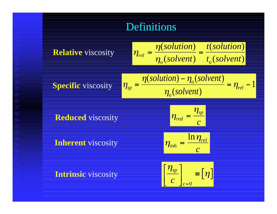
Definitions
Relative viscosity
Specific viscosity
Reduced viscosity
Inherent viscosity
Intrinsic viscosity
ηηηrel
o o
solution
solvent
t solution
t solvent= =
( )( )
( )( )
ηη η
ηηsp
o
orel
solution solvent
solvent=
−= −
( ) ( )( )
1
ηη
inhrel
c=
ln
ηη
redsp
c=
ηηsp
cc
≡ [ ]
=0
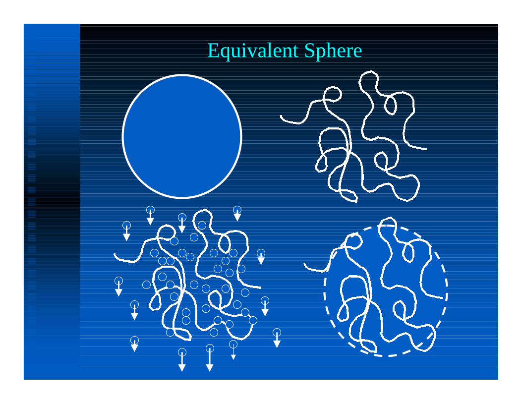
Equivalent Sphere
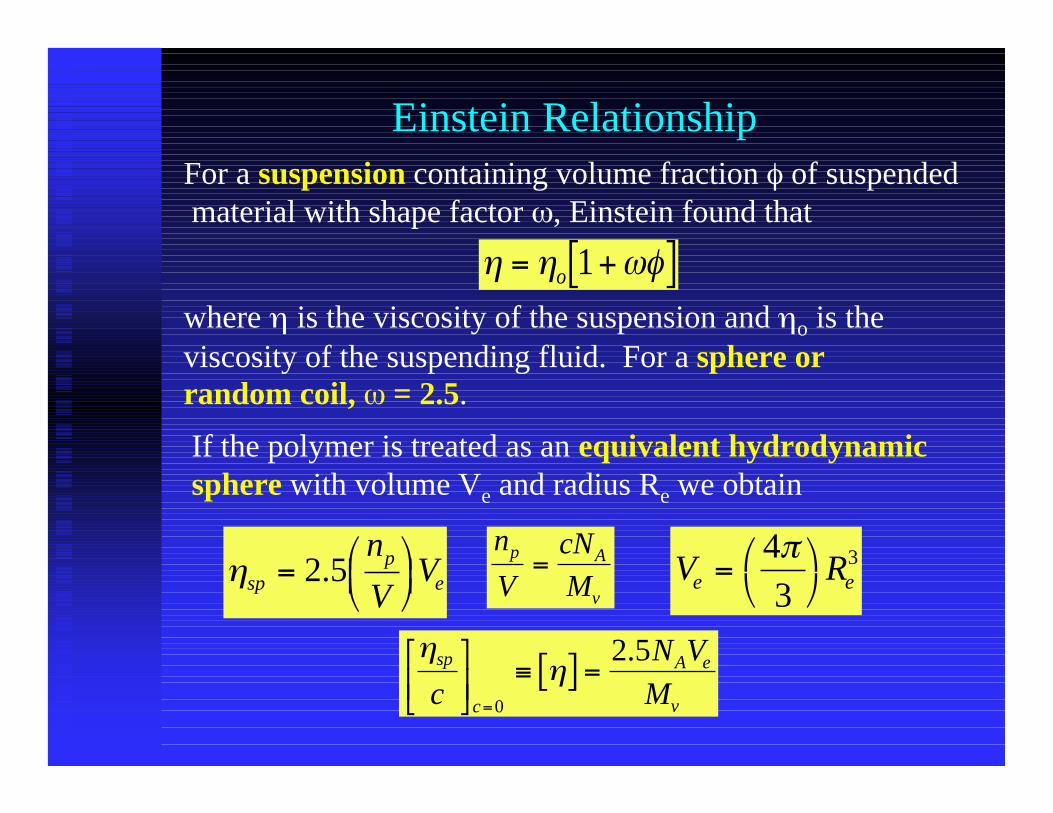
Einstein Relationship
η η ωφ= +[ ]o 1
For a suspension containing volume fraction φ of suspended material with shape factor ω, Einstein found that
where η is the viscosity of the suspension and ηo is theviscosity of the suspending fluid. For a sphere orrandom coil, ω = 2.5.
If the polymer is treated as an equivalent hydrodynamicsphere with volume Ve and radius Re we obtain
ηspp
e
n
VV=
2 5. V Re e=
43
3πn
V
cN
Mp A
v
=
ηηsp
c
A e
vc
N V
M
≡ [ ] =
=0
2 5.
Excluded Volume
That portion of the solution volume that is inaccessible topolymer chain segments due to prior occupancy by otherchain segments is known as the excluded volume.
As a consequence of the volume exclusion, the overallspatial dimensions of a real polymer chain must increaserelative to those predicted by the simple chain models.
One can compensate for chain expansion due to excludedvolume through placing the polymer in a poor solventsuch that interactions between polymer segments andsolvent molecules are thermodynamically unfavorable.Such a solvent, at a given temperature, is a theta solvent.
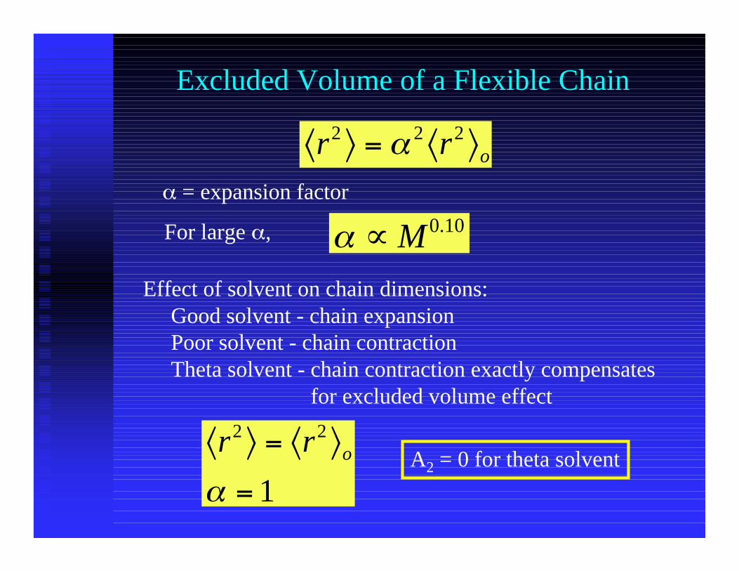
Excluded Volume of a Flexible Chain
⟨ ⟩ = ⟨ ⟩r r o2 2 2α
α = expansion factor
For large α, α ∝ M0 10.
Effect of solvent on chain dimensions: Good solvent - chain expansion Poor solvent - chain contraction Theta solvent - chain contraction exactly compensates for excluded volume effect
⟨ ⟩ = ⟨ ⟩
=
r r o2 2
1αA2 = 0 for theta solvent
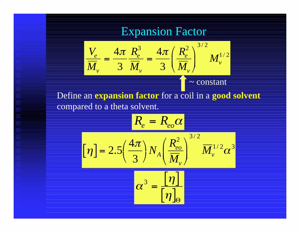
Expansion Factor
V
M
R
M
R
MMe
v
e
v
e
vv= =
43
43
3 2 3 2
1 2π π/
/
~ constant
Define an expansion factor for a coil in a good solventcompared to a theta solvent.
R Re eo= α
ηπ
α[ ] =
2 5
43
2 3 2
1 2 3./
/NR
MMA
eo
vv
αηη
3 = [ ][ ]Θ
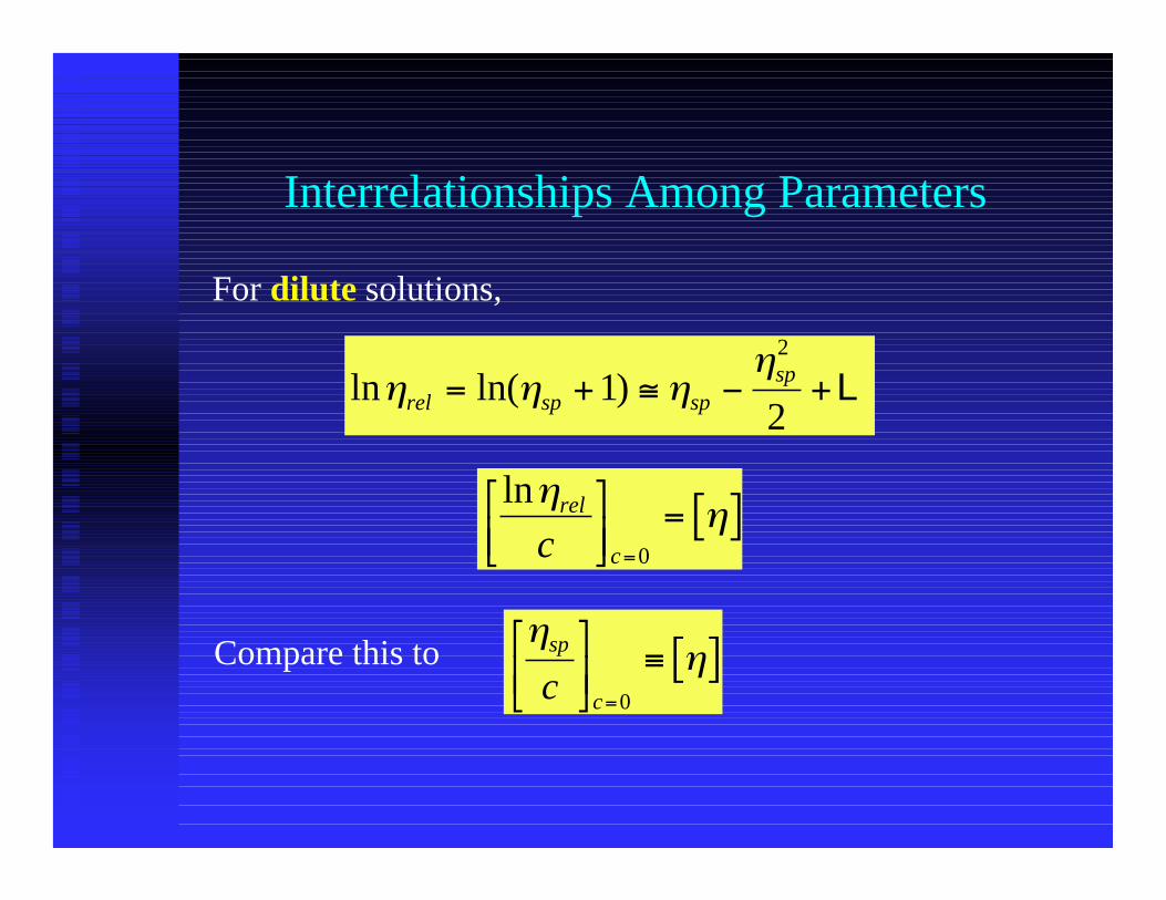
Interrelationships Among Parameters
For dilute solutions,
ln ln( )η η η
ηrel sp sp
sp= + ≅ − +12
2
L
lnηηrel
cc
= [ ]=0
ηηsp
cc
≡ [ ]
=0
Compare this to
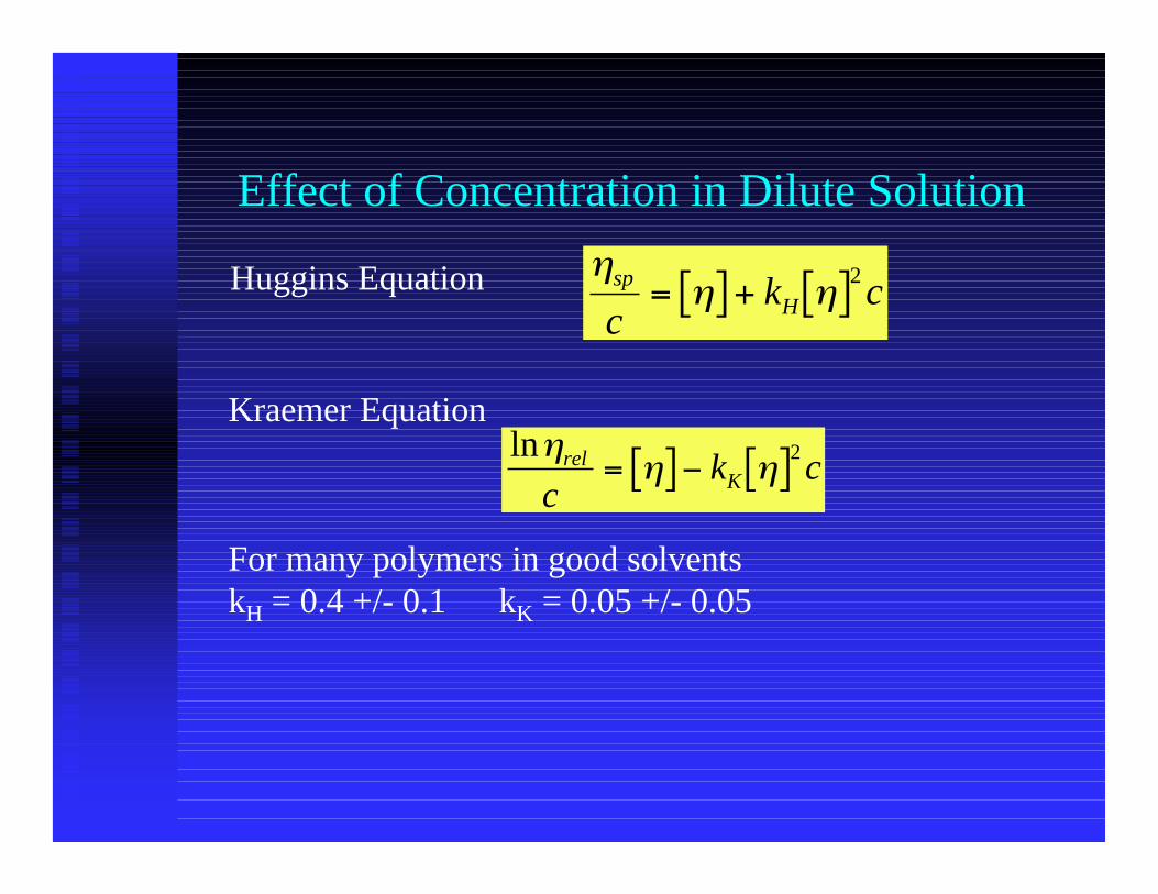
Effect of Concentration in Dilute Solution
Huggins Equation
Kraemer Equation
For many polymers in good solventskH = 0.4 +/- 0.1 kK = 0.05 +/- 0.05
ηη ηsp
Hck c= [ ] + [ ]2
lnηη ηrel
Kck c= [ ]− [ ]2
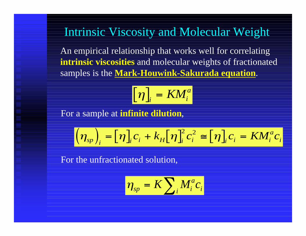
Intrinsic Viscosity and Molecular Weight
An empirical relationship that works well for correlatingintrinsic viscosities and molecular weights of fractionatedsamples is the Mark-Houwink-Sakurada equation.
η[ ] =i iaKM
For a sample at infinite dilution,
η η η ηsp i i i H i i i i ia
ic k c c KM c( ) = [ ] + [ ] ≅ [ ] =2 2
ηsp ia
i iK M c= ∑
For the unfractionated solution,
Intrinsic Viscosity and Molecular Weight
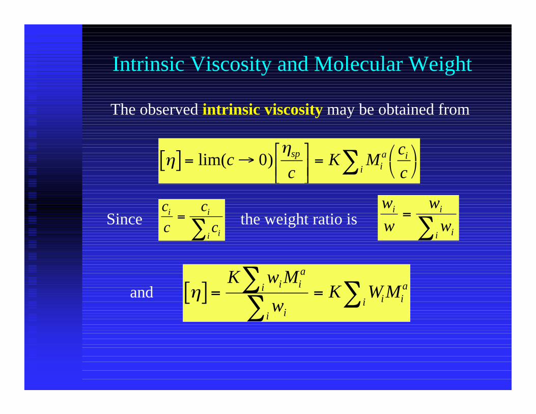
The observed intrinsic viscosity may be obtained from
ηη
[ ] = →
=
∑lim( )c
cK M
c
csp
ia
i
i0
Sincec
c
c
ci i
ii
=∑ the weight ratio is
w
w
w
wi i
ii
=∑
η[ ] = =∑∑ ∑
K w M
wK W M
i ia
i
ii
ii iaand
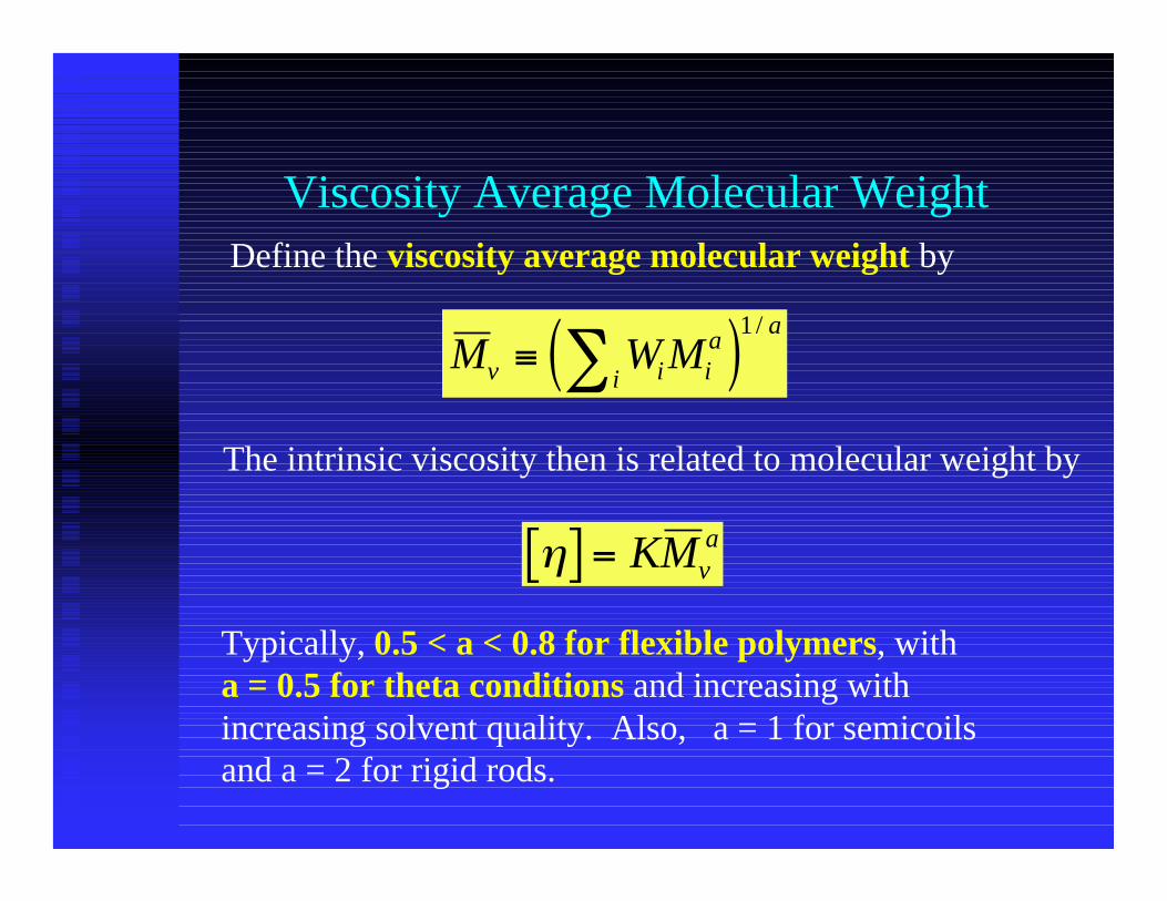
Viscosity Average Molecular Weight
M W Mv i ia
i
a≡ ( )∑
1/
Define the viscosity average molecular weight by
η[ ] = KMva
The intrinsic viscosity then is related to molecular weight by
Typically, 0.5 < a < 0.8 for flexible polymers, witha = 0.5 for theta conditions and increasing with increasing solvent quality. Also, a = 1 for semicoils and a = 2 for rigid rods.
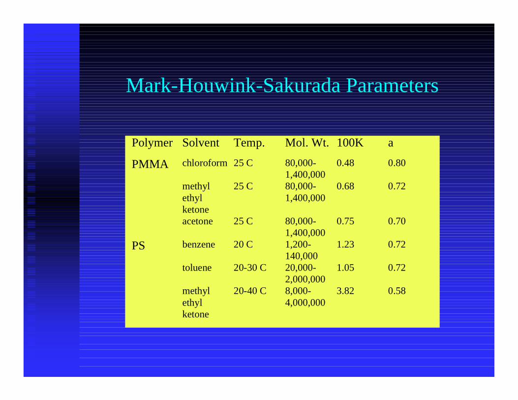
Mark-Houwink-Sakurada Parameters
Polymer Solvent Temp. Mol. Wt. 100K a
PMMA chloroform 25 C 80,000-1,400,000
0.48 0.80
methylethylketone
25 C 80,000-1,400,000
0.68 0.72
acetone 25 C 80,000-1,400,000
0.75 0.70
PS benzene 20 C 1,200-140,000
1.23 0.72
toluene 20-30 C 20,000-2,000,000
1.05 0.72
methylethylketone
20-40 C 8,000-4,000,000
3.82 0.58
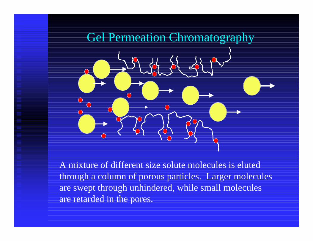
Gel Permeation Chromatography
A mixture of different size solute molecules is eluted through a column of porous particles. Larger moleculesare swept through unhindered, while small moleculesare retarded in the pores.
GPC Calibration
ηηsp
c
A e
c
N V
M
≡ [ ] =
=0
2 5.
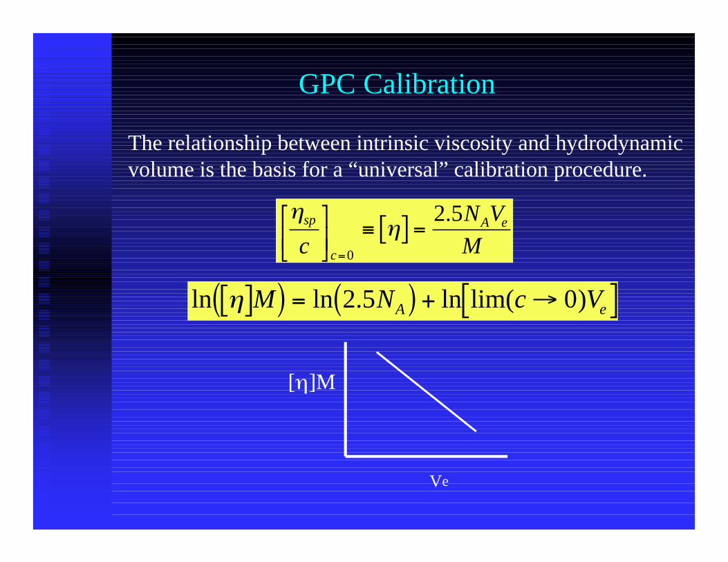
The relationship between intrinsic viscosity and hydrodynamicvolume is the basis for a “universal” calibration procedure.
ln ln . ln lim( )η[ ]( ) = ( ) + →[ ]M N c VA e2 5 0
Ve
[η]M
GPC Calibration
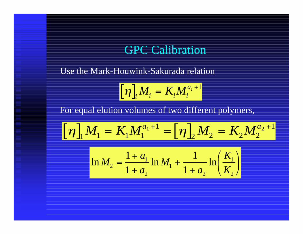
For equal elution volumes of two different polymers,
η η[ ] = = [ ] =+ +1 1 1 1
12 2 2 2
11 2M K M M K Ma a
ln ln lnMa
aM
a
K
K21
21
2
1
2
11
11
=++
++
η[ ] = +i i i i
aM K M i 1
Use the Mark-Houwink-Sakurada relation
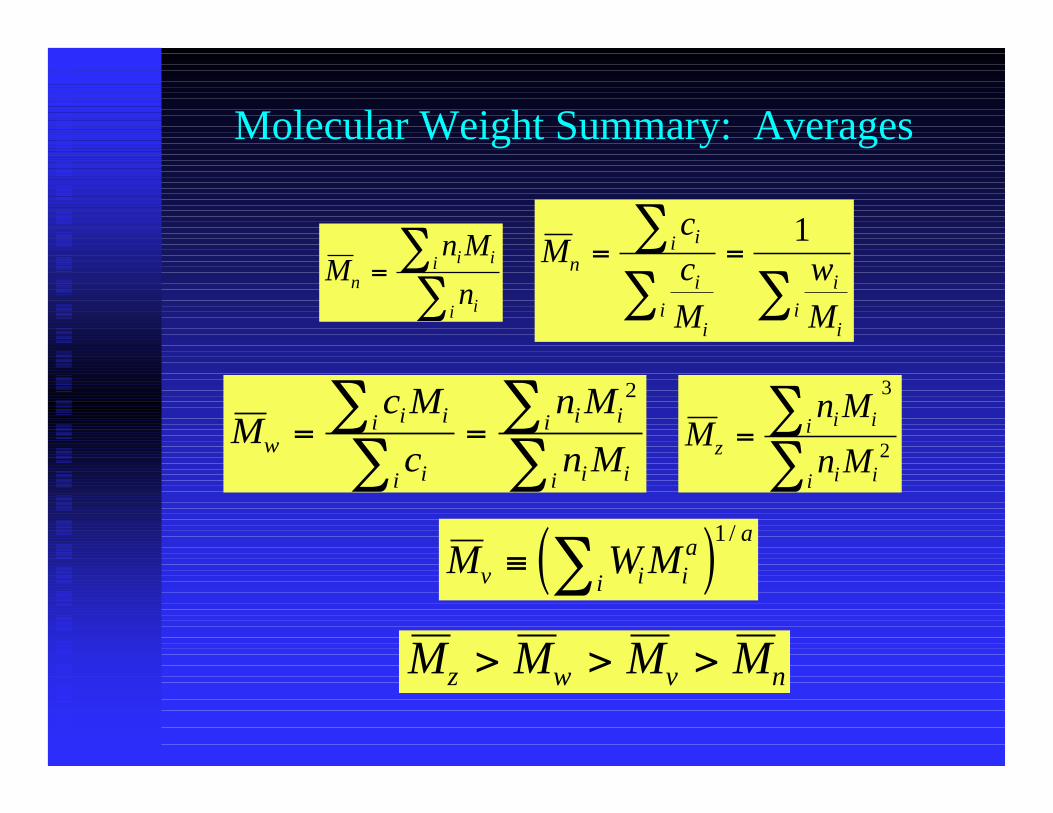
Molecular Weight Summary: Averages
M W Mv i ia
i
a≡ ( )∑
1/
Mcc
M
w
M
n
ii
i
ii
i
ii
= =∑∑ ∑
1
Mc M
c
n M
n Mw
i ii
ii
i ii
i ii
= =∑∑
∑∑
2
Mn M
n Mz
i ii
i ii
=∑∑
3
2
Mn M
nn
i ii
ii
=∑∑
M M M Mz w v n> > >
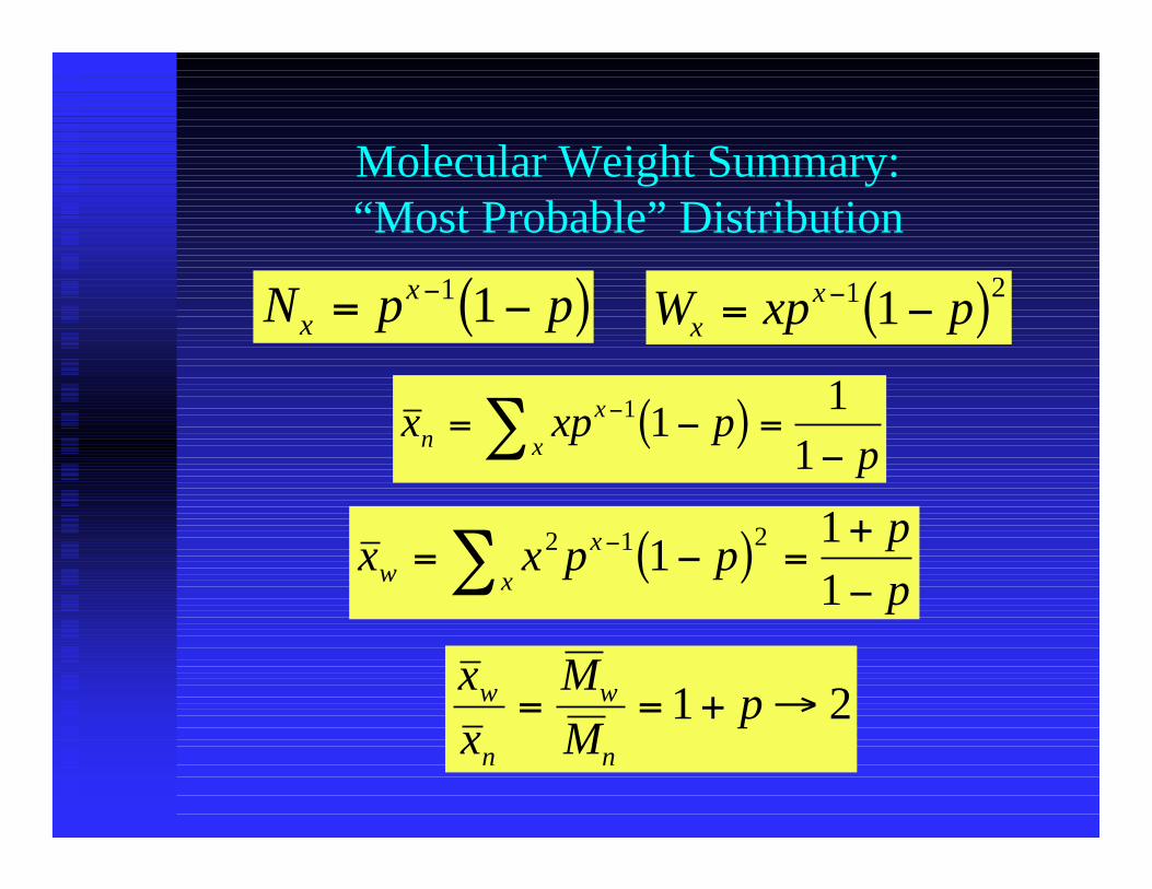
Molecular Weight Summary:“Most Probable” Distribution
x
x
M
Mpw
n
w
n
= = + →1 2
x x p pp
pwx
x= −( ) =
+−
−∑ 2 1 2111
x xp ppn
x
x= −( ) =
−−∑ 1 1
11
N p pxx= −( )−1 1 W xp px
x= −( )−1 21
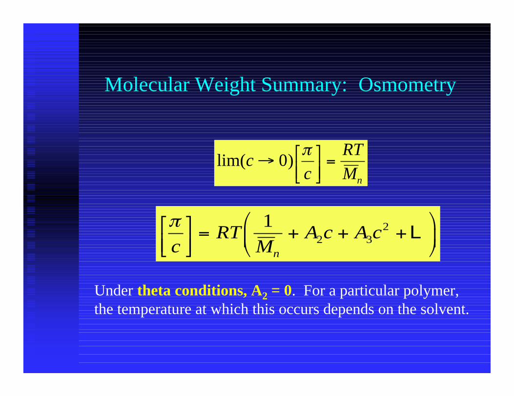
Molecular Weight Summary: Osmometry
lim( )cc
RT
Mn
→
=0
π
πc
RTM
A c A cn
= + + +
12 3
2 L
Under theta conditions, A2 = 0. For a particular polymer,the temperature at which this occurs depends on the solvent.
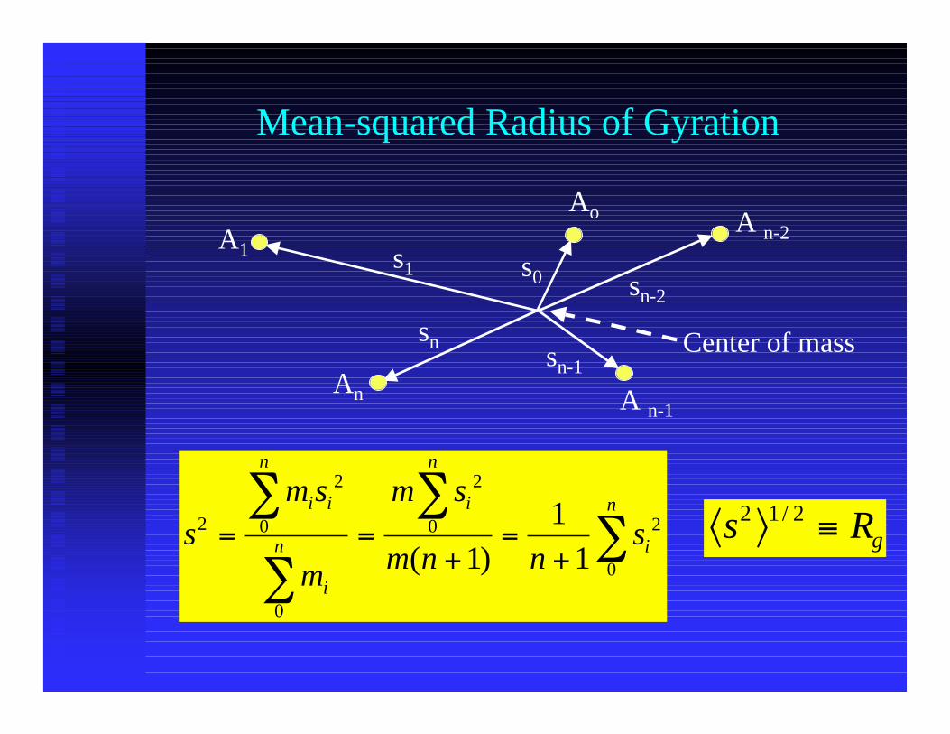
Mean-squared Radius of Gyration
sm s
m
m s
m n ns
i i
n
i
n
i
n
i
n2
2
0
0
2
0 2
011
1= =
+=
+
∑
∑
∑∑( )
A1
An
Ao
A n-1
A n-2
s1
sn
sn-2s0
sn-1Center of mass
⟨ ⟩ ≡s Rg2 1 2/
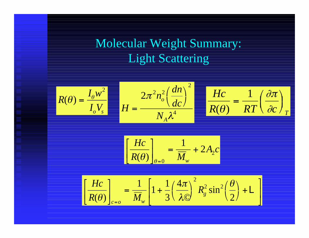
Molecular Weight Summary:Light Scattering
Hc
R MA c
w( )θ θ
= +
=0
2
12
Hc
R MR
c o wg( ) ©
sinθ
πλ
θ
= +
+
=
11
13
42
22 2 L
RI w
I Vo s
( )θ θ=2
Hn
dn
dcN
o
A
=
2 2 22
4
π
λ
Hc
R RT c T( )θ∂π∂
=
1
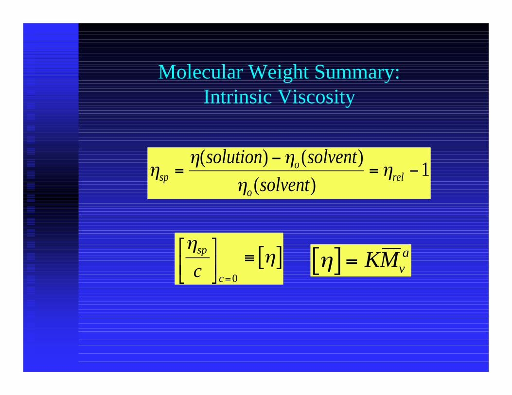
Molecular Weight Summary:Intrinsic Viscosity
η[ ] = KMva
ηη η
ηηsp
o
orel
solution solvent
solvent=
−= −
( ) ( )( )
1
ηηsp
cc
≡ [ ]
=0
Molecular Weight Summary:Gel Permeation Chromatography
ηηsp
c
A e
c
N V
M
≡ [ ] =
=0
2 5.