Lecture notes:

GE 263 – Computational Geophysics

The spectral element method

Jean-Paul Ampuero∗

Abstract

The spectral element method (SEM) is a high order numericalmethod for solving partial differential equations that inherits the ac-curacy of spectral methods and the geometrical flexibility of the finiteelement method.

These lectures provide an introduction to the SEM for graduatestudents in Earth science. The construction of the method is describedfor a model problem in 1D and 2D. The elements of its mathematicalbasis, including its connection to spectral methods, are outlined toexplain the key choices in the construction of the SEM that lead toan accurate and efficient numerical method. Practical guidelines forprogrammers and users of the SEM and entry points to advanced topicsand to the relevant applied math literature are provided.

These lectures were preceded by lectures on the finite differencemethod (FDM) and the finite element method (FEM). Several conceptsfrom the FEM lectures reappear here, with slightly different notations.We favor redundancy in the hope that the resulting exposition of keypractical aspects will contribute to attenuate the perceived complexityof programming the FEM and SEM.

These lectures were first taught in Caltech on Winter 2009.

∗California Institute of Technology, Seismological Laboratory, ampuero@caltech.edu

1

Contents

1 Overview 41.1 Overview of the spectral element method . . . . . . . . . . . 41.2 Historical perspective . . . . . . . . . . . . . . . . . . . . . . 4

2 From spectral methods to SEM, in 1D 52.1 1D model problem: Helmholtz equation . . . . . . . . . . . . 52.2 Galerkin approximation . . . . . . . . . . . . . . . . . . . . . 62.3 Spectral methods . . . . . . . . . . . . . . . . . . . . . . . . . 72.4 Numerical integration: Gauss quadrature . . . . . . . . . . . 82.5 Spectral method with numerical integration . . . . . . . . . . 92.6 The spectral element method . . . . . . . . . . . . . . . . . . 13

3 The SEM in higher dimensions 173.1 2D model problem . . . . . . . . . . . . . . . . . . . . . . . . 173.2 Spectral element mesh . . . . . . . . . . . . . . . . . . . . . . 183.3 Basis function . . . . . . . . . . . . . . . . . . . . . . . . . . . 193.4 2D integrals . . . . . . . . . . . . . . . . . . . . . . . . . . . . 193.5 Local mass matrix . . . . . . . . . . . . . . . . . . . . . . . . 203.6 Local stiffness matrix . . . . . . . . . . . . . . . . . . . . . . . 203.7 Boundary matrix . . . . . . . . . . . . . . . . . . . . . . . . . 22

4 Numerical properties 234.1 Dispersion analysis in 1D . . . . . . . . . . . . . . . . . . . . 244.2 Optimal choice of h and P . . . . . . . . . . . . . . . . . . . . 28

5 Time integration of the wave equation 315.1 Second order schemes . . . . . . . . . . . . . . . . . . . . . . 315.2 Higher-order symplectic schemes . . . . . . . . . . . . . . . . 37

6 Miscellaneous 386.1 Limitations of the SEM . . . . . . . . . . . . . . . . . . . . . 386.2 Advanced topics . . . . . . . . . . . . . . . . . . . . . . . . . 38

A References 39

B Available software 39

2

C Homework problems 40C.1 Love wave modes in a horizontally layered medium . . . . . . 40C.2 Wave propagation and numerical dispersion . . . . . . . . . . 42

3

1 Overview

1.1 Overview of the spectral element method

The SEM combines the best of two worlds: flexibility of FEM and accuracyof spectral methods.The operational procedure is similar to FEM:

1. PDE problem formulated in weak form.

2. Domain decomposition into a mesh of quadrilateral (2D) or hexaedral(3D) elements, possibly deformed.

3. Galerkin method: approximate the weak form over a finite space ofpiecewise polynomial functions

4. Evaluate the integrals in the weak form with numerical quadrature

The SEM is a high-order method : the basis functions are polynomials oforder typically ≥ 4. Among several ways to construct a high-order FEM, theSEM is characterized by an optimal choice of basis functions and quadraturerule. Optimal means less expensive (fewer operations and smaller memoryrequirement) for a given accuracy.Different than h-p FEM:

• Nodal basis instead of Modal basis

• Tensor-product basis. Each element is mapped to the reference ele-ment [−1, 1]D . In the reference element, assume a set of basis functionsmade of products of polynomials of each space variable, with degreeP : φ(x) = pi(x)pj(y)pk(z).

• diagonal matrix by choice of quadrature and interpolation nodes (butequivalent to mass lumping)

• spectral convergence (note also convergence of inter-element fluxes)

The SEM has, of course, some limitations that will be reviewed in Sec-tion 6.1.

1.2 Historical perspective

History of numerical methods for solving PDEs

• 1950s FDM

4

• 1960s FEM

• 1970s spectral methods (1965 FFT)

• 1990s SEM

• DGM?

History of SEM

• introduced by Patera (1984) on Chebyshev polynomials, for fluid dy-namics

• generalized by Maday and Patera (1989) to Legendre polynomials

• application to seismic wave propagation: Cohen et al (1993), Serianiand Priolo (1994), Faccioli et al (1997), Komatitsch and Vilotte (1998),Chaljub, Nissen-Meyer.

• application to earthquake dynamics: Ampuero (2002 +Vilotte), Festa(2004), Kaneko (2009)

• application to geophysical fluid dynamics: Taylor et al (1997, atmo-spheric model, shallow water equation on the sphere), Dupont etal (2004, ocean modeling on triangles), Fournier et al (2004, coremagneto-hydrodynamics), Rosenberg et al (2006, AMR, +Aime Fournier)

2 From spectral methods to SEM, in 1D

2.1 1D model problem: Helmholtz equation

Arises from, e.g., the wave equation in frequency domain as in waveformtomography applications. Increasing efforts are currently devoted towardsrealizing 3D waveform tomographic inversion [e.g. Bleibinhaus et al, JGR2007]. Waveform tomography is classically based on frequency domainsolvers, which do not involve time discretization.

Strong form

Given λ a real positive constant and f(x) a function of x ∈ [a, b], find u(x)such that

∂2u

∂x2+ λu + f = 0 (2.1)

5

with boundary conditions

u(a) = 0 Dirichlet (2.2)

∂u

∂x(b) = 0 Neumann (2.3)

Weak form

Define Sobolev spaces

L2([a, b]) = u : [a, b]→ R |∫ b

au(x)2 dx <∞ (2.4)

H1([a, b]) = u ∈ L2([a, b]) | du

dx∈ L2([a, b]) (2.5)

H10 ([a, b]) = u ∈ H1([a, b]) | u(a) = u(b) = 0 (2.6)

Find u ∈ H1([a, b]) such that for all test functions v ∈ H10 ([a, b]) the following

is satisfied ∫ b

a

∂v

∂x

∂u

∂xdx−

∫ b

aλvu dx =

∫ b

avf dx (2.7)

See previous lectures on FEM for proof of equivalence between strong andweak formulation. In particular, note that the boundary terms appearingafter integration-by-parts vanish, [v ∂u

∂x ]ba = 0. Equation 2.7 can be writtenas

a(u, v)− λ(u, v) = (f, v) (2.8)

where (·, ·) denotes dot product and the first term is a bilinear form a(·, ·).

2.2 Galerkin approximation

For practical implementation in a computer code, we must restrict the searchto a subspace V h ⊂ H1

0 that has finite dimension. With basis functionsφini=0. Search an aproximate solution in this subspace:

uh(x) =n∑

i=0

uiφi(x). (2.9)

Obtain the solution coefficients ui by requiring

a(uh, vh)− λ(uh, vh) = (f, vh) ∀vh ∈ V h. (2.10)

This leads to the following algebraic system of equations:

(K− λM)u = f (2.11)

6

with

Kij = a(φi, φj) (2.12)

Mij = (φi, φj) (2.13)

fi = (f, φi) (2.14)

Two important choices will be expanded next: the basis functions and thenumerical method to evaluate the integrals.

2.3 Spectral methods

The basis functions φi are polynomials of degree P that span the wholedomain. In principle, infinite modal expansion:

u(x) =

∞∑

i=0

ui φi(x) (2.15)

withui = (u, φi) (2.16)

In practice, we need truncation:

u(x) ≈ uh(x) =

P∑

i=0

ui φi(x) (2.17)

If the basis is well chosen the coefficients ui decay very fast, and trunca-tion introduces a very small error for sufficiently large P . Optimal choiceshave the spectral convergence property: for infinitely smooth functions, thetruncation error decays as a function of P faster than any power law

||u− uh|| = O(P−m) ∀m > 0 (2.18)

[Catch: spectral convergence does not hold for less smooth functions.]A family of optimal choices are the eigenfunctions of singular Sturm-Liouvilleproblems. The polynomials within this family are the so-called Jacobi poly-nomials. Legendre polynomials are a special case.The Legendre polynomials are the only sequence of polynomials Li ofdegree i that satisfy the following orthogonality conditions:

∫ 1

−1Li(ξ)Lj(ξ) dξ = δij ∀i, j = 0, 1, .... (2.19)

Cea’s lemma: The spectral convergence property also holds for the solutionof the PDE problem in weak form: ||u− uh|| is of same order as ||u− uh||.

7

2.4 Numerical integration: Gauss quadrature

In practice the integrals involved above are evaluated by numerical integra-tion (quadrature). Gaussian quadrature is based on polynomial expansions.The quadrature rule is defined by P nodes ξi and weights wi designed sothat

∫ 1

−1p(ξ) dξ =

P∑

i=0

wip(ξi) (2.20)

for all polynomials p up to a certain polynomial order.The maximum degree that can be integrated exactly by a quadrature basedon P + 1 nodes (and P + 1 weights, that’s 2P + 2 degrees of freedom) is2P + 1.

Gauss-Legendre quadrature

The optimal quadrature, i.e. one that achieves exact integration up to de-gree 2P + 1, is the so-called Gauss-Legendre quadrature rule. The Gauss-Legendre quadrature takes ξiPi=0 to be the zeros of LP+1 and the weights

wi =2

(1− ξ2i )[L

′P+1(ξi)]2

(2.21)

have been designed to give an exact quadrature up to degree P . It can beshown that the quadrature is actually exact up to degree 2P +1. (The proofrelies on the orthogonality of the Legendre polynomials.)

Gauss-Lobatto-Legendre quadrature

To enforce boundary conditions and inter-element continuity (as we willsee later) it is convenient to include the end points among the quadraturenodes. The maximum degree for exact quadrature is now 2P − 1, the P + 1quadrature nodes are the zeros of (1−ξ2)L′

P (ξ), the so-called Gauss-Lobatto-Legendre (GLL) points, and the weights are

wi =2

P (P + 1)[LP (ξi)]2(2.22)

The GLL nodes are not uniformly distributed, they tend to cluster near theend points ±1 (the inter-nodal distance near the end points is asymptotically∝ 1/P 2).

8

2.5 Spectral method with numerical integration

Discrete modal/nodal duality and spectral convergence

Let u(ξ) be a function of ξ ∈ [−1, 1]. Its Legendre expansion is

u(ξ) =

∞∑

m=0

umLm(ξ) (2.23)

where the coefficients um are the Legendre transform of u:

um = (u,Lm) =

∫ 1

−1u(ξ)Lm(ξ) dξ (2.24)

Its approximation by truncation to the first P + 1 terms:

u(ξ) ≈ u(ξ) =

P∑

m=0

umLm(ξ) (2.25)

has spectral convergence: for smooth u the misfit ||u− u|| (aka the aliasingerror) decays faster than any power law as a function of P .In practice, the integral in Equation 2.24 must be approximated by quadra-ture. Taking the GLL quadrature of order P defines a discrete (and trun-cated) Legendre transform:

u(ξ) =

P∑

m=0

umLm(ξ) (2.26)

with

um = (u,Lm)P =

P∑

i=0

wi u(ξi)Lm(ξi) (2.27)

Approximating u by u introduces an error of the same order as the aliasingerror between u and u. Hence, u is also a spectral approximation of u.The following identity arises from the particular choice of GLL interpolationand quadrature: u is the polynomial of degree P that interpolates u at theP GLL nodes,

u(ξi) = u(ξi). (2.28)

Hence, the modal representation in Equation 2.26 is equivalent to the fol-lowing nodal representation:

u(ξ) =

P∑

i=0

uiℓi(ξ) (2.29)

9

where the coefficients are simply the values of u at the GLL nodes

ui = u(ξi) (2.30)

and ℓiPi=0 are the Lagrange interpolation polynomials associated with theGLL nodes of order P .

Definition of the discrete spectral method

For a given order P , the method consists of:

1. map the domain x ∈ [a, b] into the reference segment ξ ∈ [−1, 1]

x =a + b

2+ h/2 ξ (2.31)

where h = b − a is the size of the domain, and formulate the weakform problem in the reference domain

2. take as basis functions, φiPi=0, the Lagrange polynomials associatedwith the P + 1 GLL nodes

ℓi(ξ) =∏

j 6=i

ξ − ξj

ξi − ξi(2.32)

[Recall ℓi are “discrete delta-functions” in the space of polynomials ofdegree P : ℓi ∈ PP ([−1, 1]) and ℓi(ξj) = δij .]

3. solve Equation 2.11 where Equation 2.12 to Equation 2.14 are evalu-ated with GLL quadrature.

The convergence of this method is spectral, even if the quadrature is ofreduced order (exact for 2P − 1 instead of 2P ). The quadrature introducesan error that is consistent with (same order as) the approximation error ofthe polynomial expansion. [Canuto and Quarteroni (1982) showed that thediscrete norm is uniformly equivalent to the continuous norm.]

10

Diagonal mass matrix

A major practical advantage: the mass matrix is diagonal by construction

Mpq = h/2 (ℓp, ℓq)P (2.33)

= h/2

P∑

i=0

wiℓp(ξi)ℓq(ξi) (2.34)

= h/2

P∑

i=0

wi δpi δqi (2.35)

= h/2 wp δpq (2.36)

What if we had evaluated the mass matrix with exact integration? Must

be done with a different quadrature, with Q+1 quadrature nodes ξ(Q)i

Qi=0

and weights w(Q)i

Qi=0, exact at least up to degree 2P (instead of 2P −1 for

GLL with P +1 nodes). GLL quadrature with Q = P +1 or GL quadraturewith Q = P − 1 would work.

M exactpq = h/2

Q∑

i=0

w(Q)i ℓ(P )

p (ξ(Q)i ) ℓ(P )

q (ξ(Q)i ) (2.37)

The ℓ terms here are 6= 0, because the values are requested at nodes thatare not the nodes that define the ℓ’s. Hence, the exact mass matrix is full:M exact

pq 6= 0 for all p, q.The spectral mass matrix can also be obtained by lumping the exact massmatrix, a typical trick in FEM. The sum of the p-th row of the exact massmatrix is:

P∑

q=0

M exactpq =

P∑

q=0

(ℓp, ℓq) (2.38)

=

ℓp,

P∑

q=0

ℓq

(2.39)

= (ℓp, 1) (2.40)

= wp δpq (2.41)

11

Stiffness matrix

The stiffness matrix is full.

Kpq = 2/h (ℓ′p, ℓ′q)P (2.42)

= 2/hP∑

i=0

wi ℓ′p(ξi) ℓ′q(ξi) (2.43)

Introducing the matrix of derivatives of the Lagrange polynomials H suchthat

Hij = ℓ′i(ξj) (2.44)

and the diagonal matrix of quadrature weights W such that

Wij = wiδij (2.45)

we get the compact expression

K = 2/h HWHt (2.46)

Conditioning of a matrix A is important for the efficiency of iterative solversof algebraic systems y = Ax. The conditioning of the spectral stiffnessmatrix is much better (∝ P ) than that obtained with more naive choicesof basis functions (∝ 10P for regularly spaced nodes or modal expansion,Karniadakis 2.3.3.2).

Forcing vector

fp = h/2 (f, ℓp)P (2.47)

= h/2

P∑

i=0

wif(ξi)ℓp(ξi) (2.48)

= h/2

P∑

i=0

wif(ξi)δpi (2.49)

= h/2 wpf(ξp) (2.50)

(2.51)

12

Non uniform material properties

Consider the 1D SH wave equation, in frequency domain, with non uniformshear modulus µ(x) and density ρ(x):

∂

∂x

(

µ∂u

∂x

)

+ ω2ρu + f = 0 (2.52)

The mass matrix isMpq = h/2wp ρ(ξp) δpq (2.53)

For the stiffness matrix Equation 2.46 still applies if we define

Wij = wi µ(ξi) δij (2.54)

Exercise 1: Love wave modes in a layered medium

2.6 The spectral element method

Basis functions that span the whole domain are not practical for compli-cated geometries (e.g. seismic wave propagation in a sedimentary basin) ormodels with discontinuous physical properties (e.g. wave equation in layeredmedia). The approach, borrowed from FEM, is to decompose the domaininto elements, then apply a spectral method within each element. The con-tinuity of the solution across inter-element boundaries is efficiently achievedby the choice of Lobatto nodes.

The spectral element mesh

The domain [a, b] is partitioned into N elements Ωe = [Xe−1,Xe], e =1, ..., N , with X0 = a and XN = b.A mapping χe is defined between each element (x ∈ Ωe) and the referenceelement (ξ ∈ [−1, 1]):

x = χe(ξ) =1− ξ

2Xe−1 +

1 + ξ

2Xe, ξ ∈ [−1, 1] (2.55)

or, inversely,

ξ = (χe)−1(x) = 2x− (Xe−1 + Xe)/2

Xe −Xe−1, x ∈ Ωe (2.56)

Each element is provided with a GLL sub-grid. The i-th GLL node of thee-th element is located at

xei = χe(ξi) (2.57)

13

The non-redundant list of these nodes (i.e. inter-element nodes counted onlyonce) form a set of N × P + 1 global nodes

xI = xei with I = I(i, e) = (e− 1)P + i. (2.58)

The table I(i, e) is the local-to-global index map table. We adopt the fol-lowing shortcut notation for this association between indices:

I ≡ (i, e) (2.59)

The assembly operator

Consider a set of local quantities defined on an element-by-element basis:a set of local vectors aeNe=1 of size P + 1 each, or a set of local matricesAeNe=1 of size (P + 1)× (P + 1) each.To assemble is to add the local contributions from each element into a globalarray. The assembled vector

a =NA

e=1ae, (2.60)

of size NP + 1, by definition has the following components

aI =∑

(i,e)I≡(i,e)

aei (2.61)

=

aei if I ≡ (i, e) with i ∈ [1, P − 1]

(if I is an interior node)

ae−1P + ae

0 if I ≡ (P, e− 1) ≡ (0, e)(if I is a boundary node)

(2.62)

[Figure here]. The following pseudo-code performs the assembly operation:

1 a (:) = 02 loop over e from 1 to N3 compute the local vector ae (:)4 loop over i from 0 to P5 k = I(i ,e)6 a(k) = a(k) + ae(i)7 end loop over i8 end loop over e

The components of an assembled matrix,

A =NA

e=1Ae, (2.63)

14

of size (NP + 1)× (NP + 1), are

AIJ =∑

(i,j,e)I≡(i,e)J≡(j,e)

Aeij (2.64)

=

Aeij if I ≡ (i, e) with i ∈ [1, P − 1]

or J ≡ (j, e) with j ∈ [1, P − 1](if I or J are interior nodes)

Ae−1P0 + Ae

0P if I = J ≡ (P, e − 1) ≡ (0, e)(if I = J and is a boundary node)

(2.65)

[Figure here]. The following pseudo-code performs the assembly operation:

1 A(:,:) = 02 loop over e from 1 to N3 compute the local matrix Ae(:,:)4 loop over j from 0 to P5 kj = I(j ,e)6 loop over i from 0 to P7 ki = I(i ,e)8 A(ki,kj) = A(ki,kj) + Ae(i,j)9 end loop over i

10 end loop over j11 end loop over e

Basis functions

A set of global basis functions is defined by gluing together the spectral basisfunctions based on the GLL nodes of each element:

φI(x) =

ℓei (x) if I ≡ (i, e) and x ∈ Ωe

0 else(2.66)

whereℓei (x) = ℓi[(χ

e)−1(x)] for x ∈ Ωe (2.67)

[Figure here.]These basis functions are continuous across inter-element boundaries. Thisefficiently enforces the continuity of the solution. (Same as in FEM.)

15

Galerkin approximation

A Galerkin approximation based on these basis functions and numericalintegration leads to Equation 2.11 with

K =NA

e=1Ke (2.68)

M =NA

e=1Me (2.69)

f =NA

e=1f e (2.70)

where

Keij = (ℓ′i, ℓ

′j)P /(he/2) (2.71)

Meij = (ℓi, ℓj)P he/2 (2.72)

f ei = (f, ℓi)P he/2 (2.73)

The expanded expressions are similar to those found in Section 2.5. Inparticular the global mass matrix is diagonal.Evaluating integrals:

∫ b

au(x)v(x)dx =

N∑

e=1

∫

Ωe

uv dx (2.74)

=

N∑

e=1

∫ 1

−1ue(ξ)ve(ξ) dξ he/2 (2.75)

where ue(ξ) = u|Ωe(χe(ξ)). So,

(u, v)P =N∑

e=1

(ue, ve)P he/2 (2.76)

Note that

φeI(ξ) =

ℓi(ξ) if ∃i | I ≡ (i, e)(if node I belongs to element e)

0 else(2.77)

16

The mass matrix:

MIJ = (φI , φJ)P (2.78)

=

N∑

e=1

(φeI , φ

eJ )P he/2 (2.79)

=∑

(i,j,e)I≡(i,e)J≡(j,e)

(ℓi, ℓj)P he/2 (2.80)

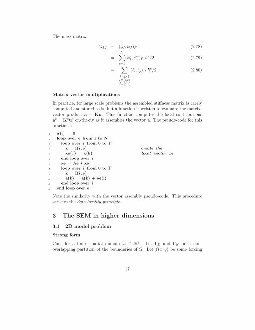
Matrix-vector multiplications

In practice, for large scale problems the assembled stiffness matrix is rarelycomputed and stored as is, but a function is written to evaluate the matrix-vector product a = Ku. This function computes the local contributionsae = Keue on-the-fly as it assembles the vector a. The pseudo-code for thisfunction is:

1 a (:) = 02 loop over e from 1 to N3 loop over i from 0 to P4 k = I(i ,e) create the

5 xe(i) = x(k) local vector xe

6 end loop over i7 ae = Ae ∗ xe8 loop over i from 0 to P9 k = I(i ,e)

10 a(k) = a(k) + ae(i)11 end loop over i12 end loop over e

Note the similarity with the vector assembly pseudo-code. This proceduresatisfies the data locality principle.

3 The SEM in higher dimensions

3.1 2D model problem

Strong form

Consider a finite spatial domain Ω ∈ R2. Let ΓD and ΓN be a non-

overlapping partition of the boundaries of Ω. Let f(x, y) be some forcing

17

function. Let ∇ denote the gradient operator, and n the outward normal toa boundary.The 2D Helmholtz model problem is:Find u(x, y) with (x, y) ∈ Ω such that

∂2u

∂x2+

∂2u

∂y2+ λu + f(x, y) = 0 (3.1)

with homogeneous Dirichlet and Neumann conditions

u(x, y) = 0 for (x, y) ∈ ΓD (3.2)

∇u(x, y) · n = 0 for (x, y) ∈ ΓN (3.3)

(3.4)

Weak form

Find u ∈ H01 (Ω) such that for all v ∈ H0

1 (Ω) we have

a(u, v)− λ(u, v) = (f, v) (3.5)

where the bilinear form is

a(u, v) =

∫ ∫

Ω∇u · ∇v dx dy (3.6)

Galerkin approximation and discrete problem

Again, find u (vector of size equal to the number of global nodes, i.e. lengthof the non-redundant list of GLL nodes) such that:

(K− λM)u = f (3.7)

with

Kij = a(φi, φj) (3.8)

Mij = (φi, φj) (3.9)

fi = (f, φi) (3.10)

3.2 Spectral element mesh

In 2D: quad elements, possibly deformed, typically Q4 (linearly deformed)or Q9 (quadratically deformed). The mesh can be unstructured. This isquite flexible, but not as much as with triangular elements. [Figures here.]

18

Local-to-global coordinate mapping (x, y) = χe(ξ, η) with (ξ, η) ∈ [−1, 1]2.Each element is endowed with a spectral grid, (P +1)2 nodes, tensor-product

of the 1D GLL nodes ξ(P )i Pi=0:

(ξi, ηj).= (ξ

(P )i , ξ

(P )j ) with i, j = 0, ..., P (3.11)

3.3 Basis function

Tensor-product basis functions. Locally:

φeI(ξ, η) = ℓi(ξ) ℓj(η) (3.12)

with I = i + j(P + 1) the lexicographic local index map. We will denoteI ≡ (i, j). [Figure here.]

3.4 2D integrals

Integral in the reference element = [−1, 1]2:

∫ ∫

u(ξ, η) dξdη =

∫ 1

−1

∫ 1

−1u(ξ, η) dξ

dη (3.13)

≈P∑

i=0

wi

P∑

j=0

wj u(ξi, ηj)

(3.14)

≈P∑

i=0

P∑

j=0

wiwj u(ξi, ηj) (3.15)

Jacobian of the inverse map for element e:

J e(ξ, η) =

∣∣∣∣∣

∂x∂ξ

∂x∂η

∂y∂ξ

∂y∂η

∣∣∣∣∣=

∂x

∂ξ

∂y

∂η− ∂y

∂ξ

∂x

∂η(3.16)

Local integral term, element e:

∫ ∫

Ωe

u(x, y) dx dy =

∫ ∫

ue(ξ, η)J e(ξ, η) dξdη (3.17)

≈P∑

i=0

P∑

j=0

wiwj u(ξi, ηj)J eij (3.18)

where J eij = J e(ξi, ηj).

19

3.5 Local mass matrix

Assembly operations apply as in the 1D case. Let’s consider only the localcontribution from element e. The local matrix component associated tonodes I ≡ (i, j) and K ≡ (k, l) is

MeIK = (φe

I , φeK)P (3.19)

Applying the 2D GLL quadrature:

MeIK =

P∑

m=0

P∑

n=0

wmwn[φeIφ

eKJ e](ξm,ηn) (3.20)

=P∑

m=0

P∑

n=0

wmwn ℓi(ξm)ℓj(ηn) ℓk(ξm)ℓl(ηn) J eij (3.21)

=

P∑

m=0

P∑

n=0

wmwnJ eij δim δjn δkm δln (3.22)

= wiwjJ eij δik δjl (3.23)

= wiwjJ eij δIK (3.24)

Again, the mass matrix is diagonal by design.

3.6 Local stiffness matrix

The local contribution from element e to the stiffness matrix is the integral

ae(φI , φK) =

∫ ∫

Ωe

(∂φI

∂x

∂φK

∂x+

∂φI

∂y

∂φK

∂y

)

dx dy (3.25)

evaluated with the GLL quadrature. This requires a change of variables tothe reference element with local coordinate system (ξ, η). Applying thechain rule for differentiation:

∂φI

∂x

∂φK

∂x+

∂φI

∂y

∂φK

∂y=

2∑

k=1

∑

α=ξ,η

∂φeI

∂α

∂α

∂xk

∑

β=ξ,η

∂φeK

∂β

∂β

∂xk

(3.26)

=∑

α

∑

β

∂φeI

∂α

∂φeK

∂β

(2∑

k=1

∂α

∂xk

∂β

∂xk

)

(3.27)

Four terms are involved:

Ke =∑

α

∑

β

Ke (αβ) (3.28)

20

with

Ke (αβ)IJ =

P∑

p=0

P∑

q=0

W (αβ)pq

[∂φe

I

∂α

∂φeK

∂β

]

(ξp,ηq)

(3.29)

where

W (αβ)pq = wpwqJ e

pq

[2∑

k=1

∂α

∂xk

∂β

∂xk

]

(ξp,ηq)

(3.30)

If we were to use these (P + 1)2 × (P + 1)2 matrices as is to evaluate Keue

we would need (P + 1)4 multiplications per element. There is however ahuge gain to make by exploiting the particular structure of the SEM. Thelocal stiffness matrix can be rewritten as

Ke (ξξ)IJ =

∑

p

∑

q

W (ξξ)pq

∂φeI

∂ξ(ξp, ηq)

∂φeJ

∂ξ(ξp, ηq) (3.31)

=∑

p

∑

q

W (ξξ)pq ℓ′i(ξp) ℓj(ηq)

︸ ︷︷ ︸

δjq

ℓ′k(ξp) ℓl(ηq)︸ ︷︷ ︸

δlq

(3.32)

= δjl

∑

p

W(ξξ)pj Hip Hkp (3.33)

where H is the matrix of derivatives of the Lagrange basis functions (Equa-tion 2.44). The matrix Ke (ξξ) is very sparse: node I ≡ (i, j) interacts onlywith nodes in column j. [Figure here.] Efficiency of tensor-product basis,low operation count compared to hp-FEM.Matrix-vector multiplication:

Fe (ξξ) = Ke (ξξ) ue (3.34)

Fe (ξξ)I =

∑

J

Ke (ξξ)IJ ue

J (3.35)

=∑

k

∑

l

Ke (ξξ)I (kl) u

ekl (3.36)

=∑

k

∑

l

δjl

∑

p

W(ξξ)pj Hip Hkpu

ekl (3.37)

=∑

k

∑

p

Hip Hkp

∑

l

δjl W(ξξ)pj ue

kl

︸ ︷︷ ︸

W(ξξ)pj ue

kj

(3.38)

=∑

p

Hip W(ξξ)pj

∑

k

Hkp uekj (3.39)

21

Let’s store the vector Fe in matrix form: we define the matrix [Fe] with size(P + 1)× (P + 1) and components F e

ij such that I ≡ (i, j). Similarly defineUe as the matrix-form storage of vector ue. We get:

[

Fe (ξξ)]

= H(We (ξξ) ⊗HtUe) (3.40)

Similarly [Exercise: show it]:[

Fe (ηη)]

= (We (ηη) ⊗UeH)Ht (3.41)[

Fe (ξη)]

= H(We (ξη) ⊗UeH) (3.42)[

Fe (ηξ)]

= (We (ηξ) ⊗HtUe)Ht (3.43)

In practice, to compute Fe we proceed in three steps:

1. compute local gradients (two mxm operations)

∇ξ = HtUe (3.44)

∇η = UeH (3.45)

2. evaluate component-by-component matrix multiplications:

[Fξ] = We (ξξ) ⊗∇ξ + We (ξη) ⊗∇η (3.46)

[Fη] = We (ηη) ⊗∇η + We (ηξ) ⊗∇ξ (3.47)

3. compute (two mxm operations)

[Fe] = H [Fξ] + [Fη]Ht (3.48)

These steps are the core of any SEM code. They involve 4 matrix-matrixmultiplications (mxm operations) that can be highly optimized. All matricesinvolved have size (P + 1)× (P + 1). The floating point operation count inthe 2D SEM is of order (P +1)3, much more efficient than the order (P +1)4

flops count in the FEM. In 3D the relative efficiency is still more dramatic:(P + 1)4 flops for the SEM versus (P + 1)6 for the FEM.

3.7 Boundary matrix

If the boundary condition is non zero on the Neumann boundary an addi-tional term appears in the weak form:

a(u, v) − λ(u, v) = (f, v) + (τ, v)ΓN(3.49)

22

where

(τ, v)ΓN=

∫

ΓN

τ(x, y) v(x, y) ds (3.50)

involves the tractions τ on the Neumann boundary ΓN . The boundary isnaturally partitioned into boundary elements, which are edges of the spectralelements. The contribution from boundary element b to the integral is

(τ, v)bΓN=

∫ 1

−1τ b(s) vb(s)J b (1D)(s) ds (3.51)

where vb is the trace of v on the b-th boundary element, mapped to a localcurvilinear coordinate s, and the 1D Jacobian is

J b (1D) =

√(

∂x

∂α

)2

+

(∂y

∂α

)2

(3.52)

where α is ξ or η if the boundary element corresponds to the element edgewith η = ±1 or ξ = ±1, respectively.Upon discretization this leads to

(K− λM)u = f + Bτ (3.53)

The vector τ involves only the nodes on the boundary ΓN . The boundarymatrix B is diagonal. At the boundary element level:

Bbij = wiJ b (1D)

i δij (3.54)

4 Numerical properties

Wave equation: dispersion and stability analysis, cost-accuracy trade-off,choice of h and P .Numerical methods for wave propagation introduce two main intrinsic er-rors: dispersion and dissipation. For a monochromatic plane wave these aredefined as the phase error and the amplitude error, respectively. In thisstudy we focus on dispersion errors for two reasons. First, when combinedwith non dissipative timestepping the SEM introduces virtually no numer-ical attenuation (exactly zero attenuation on element vertices). Second, atvery long propagation distances the numerical errors in synthetic waveformsare dominated by the mismatch introduced by time delay (dispersion) errors,a phenomenon known in the FEM litterature as the pollution effect.

23

For the sake of clarity, we will consider a non-dispersive medium with wavespeed c governed by the scalar wave equation, and a monochromatic planewave with frequency ω and wavenumber k = ω/c. The phase velocity ω/kof the numerical solution is generally different than c. We quantify thedispersion error by the relative phase velocity misfit between the numericaland the theoretical wave solutions:

ǫ.= −ω/k − c

c. (4.1)

For frequency domain problems, we will see that ǫ depends on the SEMpolynomial order P and on the non-dimensional number κ = kh, where h isthe element size. Later on, for time domain problems we will see that timediscretization introduces an additional error that depends on the order q ofthe time integration scheme and on Ω = ω∆t, where ∆t is the time step.In practice, we can measure the time delay misfit ∆T between a syntheticseismogram and the exact analytical solution (e.g. by sub-sample precisioncross-correlation time delay estimate). The dispersion error ǫ is related tothe time delay by

ǫ =∆T

T(4.2)

Because the phase velocity error ǫ is independent of T , Equation 4.2 impliesthat the time delay grows proportionally to the travel time.The average number of GLL nodes per wavelength, G, is defined by

G.= pλ/h = 2π p/kh, (4.3)

4.1 Dispersion analysis in 1D

Consider an infinite 1D medium with uniform wave speed c, discretized bya regular mesh of spectral elements with equal size h. Consider the scalarwave propagation problem in the frequency (ω) domain.In a non dispersive medium ω/k = c, but waves in the semi-discrete problemfollow a non-linear numerical dispersion relation of the form (?):

cos(kh) = RP (ωh/c) (4.4)

where RP is a rational function (a ratio of polynomials) which coefficientsdepend on the spectral order P . A compact expression for RP is given by? for the FEM of arbitrary order P . However, no similar expression is yetavailable for the SEM. Closed forms of RP for low orders are derived in

24

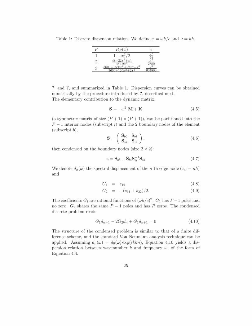
Table 1: Discrete dispersion relation. We define x = ωh/c and κ = kh.

P RP (x) ǫ

1 1− x2/2 κ2

24

2 48−22x2+x4

48+2x2κ4

2880

3 3600−1680x2+92x4−x6

3600+120x2+2x4κ6

604800

? and ?, and summarized in Table 1. Dispersion curves can be obtainednumerically by the procedure introduced by ?, described next.The elementary contribution to the dynamic matrix,

S = −ω2 M + K (4.5)

(a symmetric matrix of size (P + 1)× (P + 1)), can be partitioned into theP − 1 interior nodes (subscript i) and the 2 boundary nodes of the element(subscript b),

S =

(Sbb Sbi

Sib Sii

)

, (4.6)

then condensed on the boundary nodes (size 2× 2):

s = Sbb − SbiS−1ii Sib (4.7)

We denote dn(ω) the spectral displacement of the n-th edge node (xn = nh)and

G1 = s12 (4.8)

G2 = −(s11 + s22)/2. (4.9)

The coefficients Gi are rational functions of (ωh/c)2. G1 has P −1 poles andno zero. G2 shares the same P − 1 poles and has P zeros. The condenseddiscrete problem reads

G1dn−1 − 2G2dn + G1dn+1 = 0 (4.10)

The structure of the condensed problem is similar to that of a finite dif-ference scheme, and the standard Von Neumann analysis technique can beapplied. Assuming dn(ω) = d0(ω) exp(ikhn), Equation 4.10 yields a dis-persion relation between wavenumber k and frequency ω, of the form ofEquation 4.4.

25

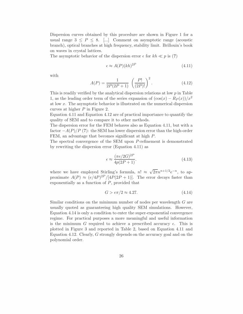
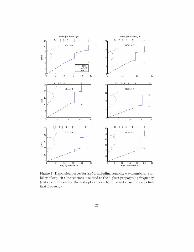
Dispersion curves obtained by this procedure are shown in Figure 1 for ausual range 3 ≤ P ≤ 8. [...] Comment on asymptotic range (acousticbranch), optical branches at high frequency, stability limit. Brillouin’s bookon waves in crystal lattices.The asymptotic behavior of the dispersion error ǫ for kh≪ p is (?)

ǫ ≈ A(P )(kh)2P (4.11)

with

A(P ) =1

2P (2P + 1)

(P !

(2P )!

)2

. (4.12)

This is readily verified by the analytical dispersion relations at low p in Table1, as the leading order term of the series expansion of (cos(x)− RP (x))/x2

at low x. The asymptotic behavior is illustrated on the numerical dispersioncurves at higher P in Figure 2.Equation 4.11 and Equation 4.12 are of practical importance to quantify thequality of SEM and to compare it to other methods.The dispersion error for the FEM behaves also as Equation 4.11, but with afactor −A(P )/P (?): the SEM has lower dispersion error than the high-orderFEM, an advantage that becomes significant at high P .The spectral convergence of the SEM upon P -refinement is demonstratedby rewriting the dispersion error (Equation 4.11) as

ǫ ≈ (πe/2G)2P

4p(2P + 1). (4.13)

where we have employed Stirling’s formula, n! ≈√

2πnn+1/2e−n, to ap-proximate A(P ) ≈ (e/4P )2P /[4P (2P + 1)]. The error decays faster thanexponentially as a function of P , provided that

G > eπ/2 ≈ 4.27. (4.14)

Similar conditions on the minimum number of nodes per wavelength G areusually quoted as guaranteeing high quality SEM simulations. However,Equation 4.14 is only a condition to enter the super-exponential convergenceregime. For practical purposes a more meaningful and useful informationis the minimum G required to achieve a prescribed accuracy ǫ. This isplotted in Figure 3 and reported in Table 2, based on Equation 4.11 andEquation 4.12. Clearly, G strongly depends on the accuracy goal and on thepolynomial order.

26

0 2 4 6 8 100

2

4

6

8

10

12ω

h/c

NGLL = 4

0 5 10 150

5

10

15

20

NGLL = 5

0 5 10 15 200

5

10

15

20

25

ω h

/c

NGLL = 6

0 5 10 15 200

10

20

30

40

NGLL = 7

0 5 10 15 20 250

10

20

30

40

50

Re(k h) and Im(k h)

ω h

/c

NGLL = 8

0 5 10 15 20 25 300

10

20

30

40

50

60

Re(k h) and Im(k h)

NGLL = 9

Re(k h)Im(k h)exact

10 6 5 4 3 2

Nodes per wavelength

10 6 5 4 3 2

Nodes per wavelength

10 6 5 4 3 2 10 6 5 4 3 2

10 6 5 4 3 2 10 6 5 4 3 2

Figure 1: Dispersion curves for SEM, including complex wavenumbers. Sta-bility of explicit time schemes is related to the highest propagating frequency(red circle, the end of the last optical branch). The red cross indicates halfthat frequency.

27

10−1

100

101

10−12

10−10

10−8

10−6

10−4

10−2

100

k h

∆ T

/ T

, di

sper

sion

err

or

100

101

10−8

10−7

10−6

10−5

10−4

10−3

10−2

10−1

100

Nodes per wavelength

∆ T

/ T

, di

sper

sion

err

or

456789

50 20 10 6 5 4 3 2 1 0.5

Elements per wavelength

456789

Figure 2: Dispersion error for SEM (3 ≤ P ≤ 8) as a function of wavenumberor number of elements per wavelength (right) and as a function of numberof nodes per wavelength (left). The dashed lines in the left plot are theasymptotic behavior given by Equation 4.11 and Equation 4.12.

By definition (Equation 4.2) ǫ has been normalized by the total travel time.If one prescribes instead the absolute error ∆T it appears that a largerG is needed for larger propagation distances. It is useful to express thedispersion error in terms of the dominant period T0 = ω/2π and the numberof wavelengths travelled T/T0:

ǫ =∆T

T0

/T

T0. (4.15)

With ǫX = 10−4 one could achieve for instance propagation over distancesof 100 wavelengths with numerical time delays of 1% of a wave period.For a global accuracy ǫ the numbers in Figure 3 and Table 2 are only lowerbounds as they do not account for the additional error due to time dis-cretization, studied in the next paragraph.

4.2 Optimal choice of h and P

We are concerned with the two competing goals that determine the per-formance of a simulation: maximizing accuracy while minimizing the com-putational cost. In SEM accuracy can be improved by decreasing h or by

28

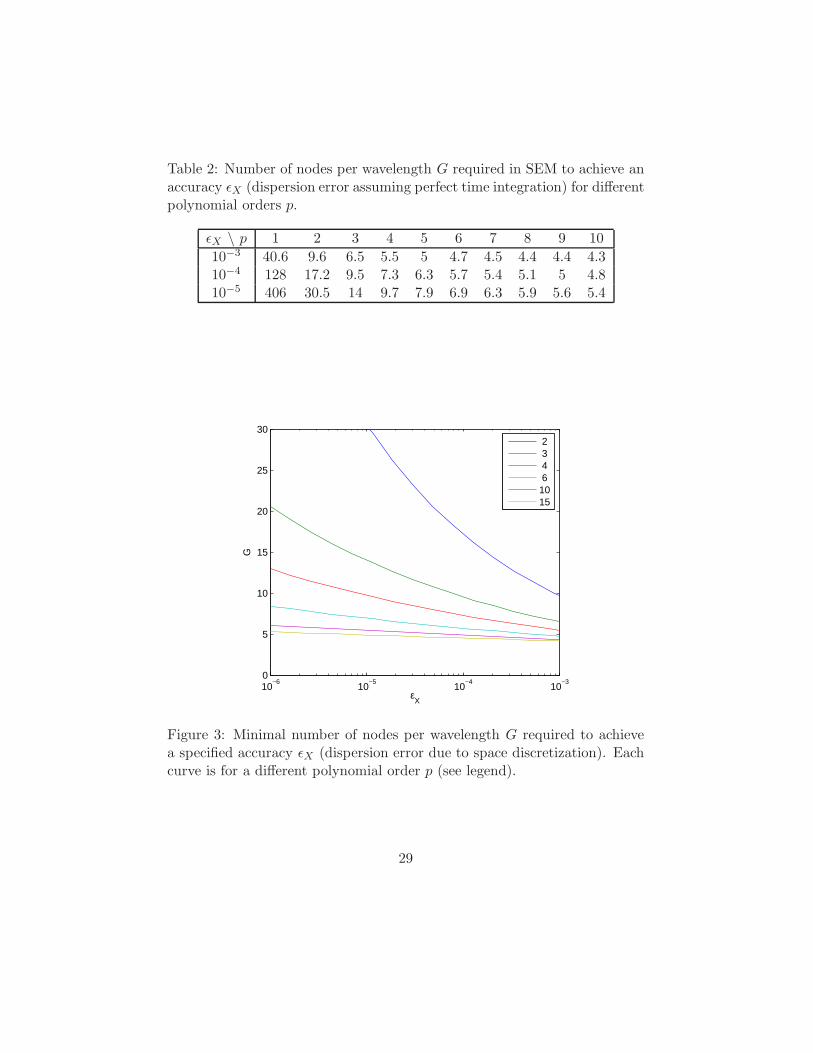
Table 2: Number of nodes per wavelength G required in SEM to achieve anaccuracy ǫX (dispersion error assuming perfect time integration) for differentpolynomial orders p.

ǫX \ p 1 2 3 4 5 6 7 8 9 10

10−3 40.6 9.6 6.5 5.5 5 4.7 4.5 4.4 4.4 4.310−4 128 17.2 9.5 7.3 6.3 5.7 5.4 5.1 5 4.810−5 406 30.5 14 9.7 7.9 6.9 6.3 5.9 5.6 5.4

10−6

10−5

10−4

10−3

0

5

10

15

20

25

30

εX

G

2 3 4 61015

Figure 3: Minimal number of nodes per wavelength G required to achievea specified accuracy ǫX (dispersion error due to space discretization). Eachcurve is for a different polynomial order p (see legend).

29

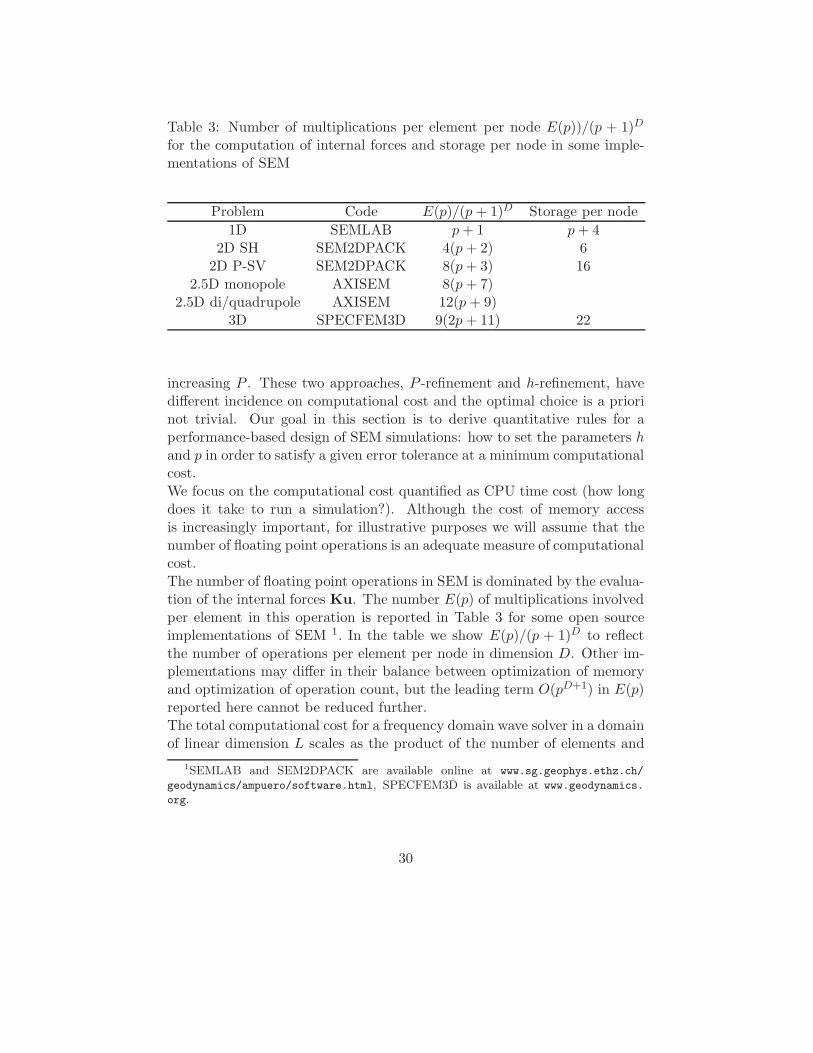
Table 3: Number of multiplications per element per node E(p))/(p + 1)D

for the computation of internal forces and storage per node in some imple-mentations of SEM

Problem Code E(p)/(p + 1)D Storage per node

1D SEMLAB p + 1 p + 42D SH SEM2DPACK 4(p + 2) 6

2D P-SV SEM2DPACK 8(p + 3) 162.5D monopole AXISEM 8(p + 7)

2.5D di/quadrupole AXISEM 12(p + 9)3D SPECFEM3D 9(2p + 11) 22

increasing P . These two approaches, P -refinement and h-refinement, havedifferent incidence on computational cost and the optimal choice is a priorinot trivial. Our goal in this section is to derive quantitative rules for aperformance-based design of SEM simulations: how to set the parameters hand p in order to satisfy a given error tolerance at a minimum computationalcost.We focus on the computational cost quantified as CPU time cost (how longdoes it take to run a simulation?). Although the cost of memory accessis increasingly important, for illustrative purposes we will assume that thenumber of floating point operations is an adequate measure of computationalcost.The number of floating point operations in SEM is dominated by the evalua-tion of the internal forces Ku. The number E(p) of multiplications involvedper element in this operation is reported in Table 3 for some open sourceimplementations of SEM 1. In the table we show E(p)/(p + 1)D to reflectthe number of operations per element per node in dimension D. Other im-plementations may differ in their balance between optimization of memoryand optimization of operation count, but the leading term O(pD+1) in E(p)reported here cannot be reduced further.The total computational cost for a frequency domain wave solver in a domainof linear dimension L scales as the product of the number of elements and

1SEMLAB and SEM2DPACK are available online at www.sg.geophys.ethz.ch/

geodynamics/ampuero/software.html, SPECFEM3D is available at www.geodynamics.

org.

30

the cost per element

cost ∝ E(P )

(L

h

)D

(4.16)

It can be rewritten ascost ∝ (kL)D × Γ, (4.17)

where

Γ =E(P )

(kh)D. (4.18)

The first term in Equation 4.17 is entirely due to the physical dimensionsof the problem whereas the term Γ encapsulates the effect of the numericalresolution. In the remainder we will refer to Γ as the computational cost.We have assumes that a good preconditioner is available, so that the numberof iterations required by the solver is practically a constant. Note that forlarge P we get

Γ ∝ (P + 1)D+1

(kh)D(4.19)

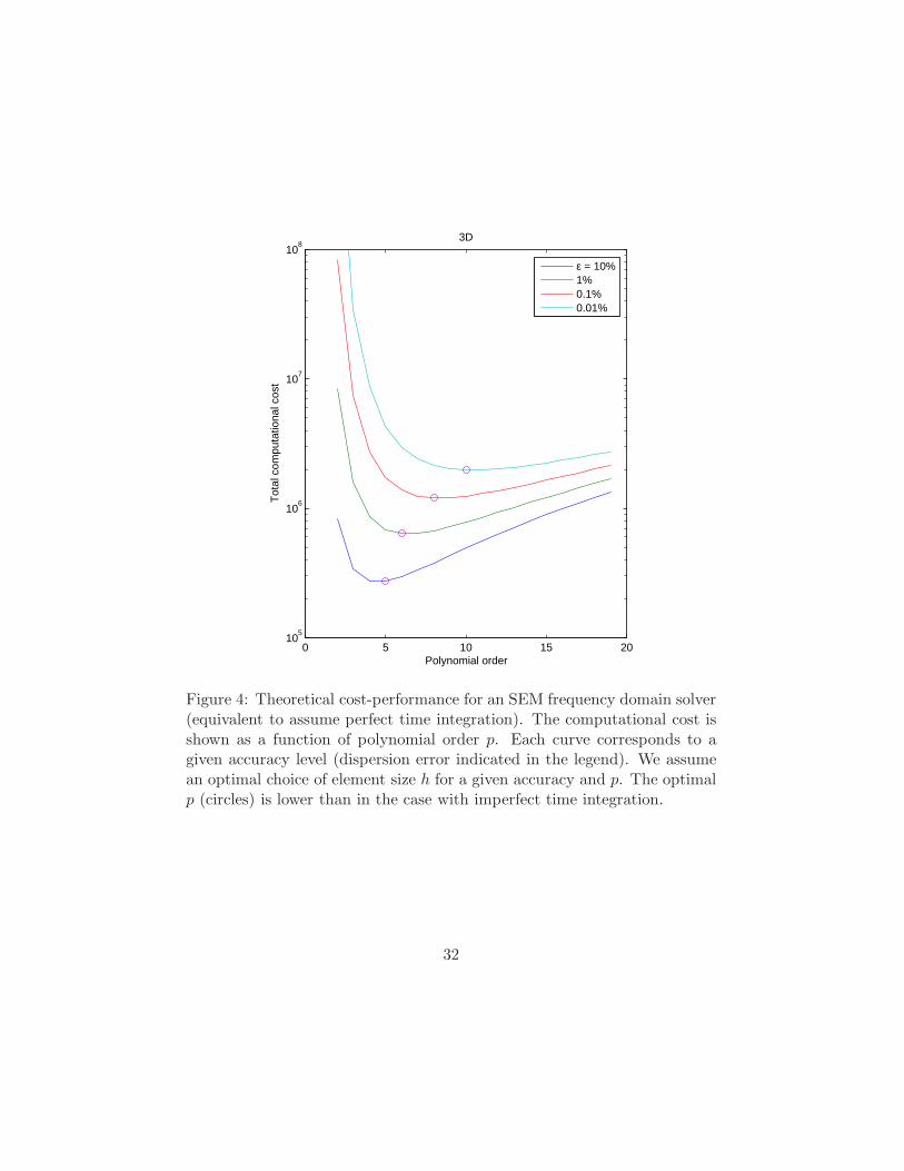
We can now address the cost-accuracy trade-offs of SEM for frequency do-main solvers. For a given accuracy level ǫ we must find the optimal valueshopt and Popt that minimize the cost function in Equation 4.18 under theconstrain of Equation 4.11 (fixed accuracy). This optimization problem issolved graphically in Figure 4, where we show the cost as a function of Pand ǫ assuming h is given by Equation 4.11. The minimum of each curve(indicated by circles) gives the optimal values of P for a given accuracy level.[Plot also the optimal h.]

5 Time integration of the wave equation

5.1 Second order schemes

Leapfrog

dn+1 = dn + ∆tvn+1/2 (5.1)

vn+3/2 = vn+1/2 + ∆tM−1[−Kdn+1 + f(tn)] (5.2)

Storage requirements: two global fields, d and v.

31

0 5 10 15 2010

5

106

107

108

3D

Tot

al c

ompu

tatio

nal c

ost

Polynomial order

ε = 10%1%0.1%0.01%

Figure 4: Theoretical cost-performance for an SEM frequency domain solver(equivalent to assume perfect time integration). The computational cost isshown as a function of polynomial order p. Each curve corresponds to agiven accuracy level (dispersion error indicated in the legend). We assumean optimal choice of element size h for a given accuracy and p. The optimalp (circles) is lower than in the case with imperfect time integration.

32

Newmark schemes

Man+1 = −Kdn+1 + f(tn+1) (5.3)

vn+1 = vn + (1− γ)∆tan + γ∆tan+1 (5.4)

dn+1 = dn + ∆tvn + (1/2 − β)∆t2 an + β∆t2 an+1 (5.5)

Predictor-corrector implementation:

1. Predictor:

d = dn + ∆tvn + (1/2 − β)∆t2 an (5.6)

v = vn + (1− γ)∆tan (5.7)

2. Solver:an+1 = M−1[−Kd + f(tn+1)] (5.8)

3. Corrector:

dn+1 = d + β∆t2 an+1 (5.9)

vn+1 = v + γ∆tan+1 (5.10)

Storage requirements: 3 global fields, d, v and a.The scheme is equivalent to leapfrog if β = 0 and γ = 1/2.The displacement update is independent of a if β = 0.

Stability

Explicit time integration schemes are conditionally stable, they are stableonly if the timestep ∆t verifies

∆t < ∆tc =C√

DΩm

h

c, (5.11)

where ∆tc is the critical timestep, D the dimension of the problem, C astability number that depends only on the time scheme and Ωm a spectralradius that depends only on the space discretization scheme. The spectralradius is the highest eigen-frequency of the dimensionless 1D wave equa-tion (c = 1) discretized by spectral elements with h = 1. In terms of thedispersion relation, Ωm is the smallest solution of

RP (Ωm) = cos(pπ) = (−1)P . (5.12)

33

Table 4: Spectral radius Ωm in SEM for different polynomial orders p.

p 1 2 3 4 5 6 7 8 9 10

Ωm 2 2√

6√

42 + 6√

29 13.55 19.80 27.38 36.27 46.42 57.87 70.6

In general Ωm is inversely proportional to the smallest node spacing. TheGauss-Lobatto-Legendre nodes of SEM are clustered at the edge of the ele-ments with spacing ∝ 1/P 2, so we expect Ωm ∝ P 2. Values for P ≤ 10 arereported in Table 4 and are well approximated (better than 1% for P ≥ 4)by

Ωm(P ) ≈ 0.64P 2 + 0.57P + 1. (5.13)

Compared to the P -FEM (?) the SEM has the advantage of a smallerspectral radius, hence larger timesteps can be used.

Accuracy

Time schemes introduce additional dispersion errors. In general dissipationerrors may also be present but we are mainly interested here in conservativeschemes. For a general scheme of order q the error behaves as

ǫ ≈ B(ω∆t)q. (5.14)

The usual leapfrog scheme is second order accurate, q = 2, and its dimen-sionless factor is B = 1/24. Within the second order class it is the mostaccurate scheme.Within the asymptotic regime, the total dispersion error combining spaceand time discretizations is

ǫ = A(P ) (kh)2P + B(ω∆t)q. (5.15)

In common practice the time step is set to a moderate fraction of the criticalvalue (5.11), i.e. ∆t = γ∆tc with γ . 1. We can write ǫ in terms of κ = khas

ǫ ≈ A(P ) κ2P + B

(γC√

DΩm(P )

)q

κq (5.16)

Both components of the dispersion error are compared in Figure 5 for P = 8.The error is dominated by the time-discretization error as soon as more than

34

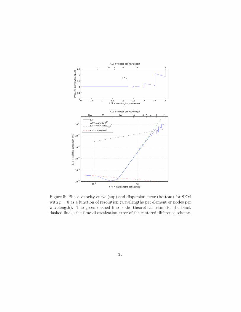
0 0.5 1 1.5 2 2.5 3 3.5 40

0.5

1

1.5

2

2.5

Pha

se v

eloc

ity /

wav

e sp

eed

h / λ = wavelengths per element

P = 8

10 6 5 4 3 2

P λ / h = nodes per wavelength

10−1

100

10−15

10−12

10−9

10−6

10−3

100

∆T /

T =

rel

ativ

e di

sper

sion

err

or

h / λ = wavelengths per element

∆T/T

∆T/T = A(p) (kh)2P

∆T/T = B (C kh/Ωmax

)2

∆T/T ∼ round−off

100 50 20 10 6 5 4 3 2

P λ / h = nodes per wavelength

Figure 5: Phase velocity curve (top) and dispersion error (bottom) for SEMwith p = 8 as a function of resolution (wavelengths per element or nodes perwavelength). The green dashed line is the theoretical estimate, the blackdashed line is the time-discretization error of the centered difference scheme.

35

10−6

10−5

10−4

10−3

10−2

10−1

10−4

10−3

10−2

εX

ε T

p=2

p=19

G = 4.5

5

6

10

εT = ε

X

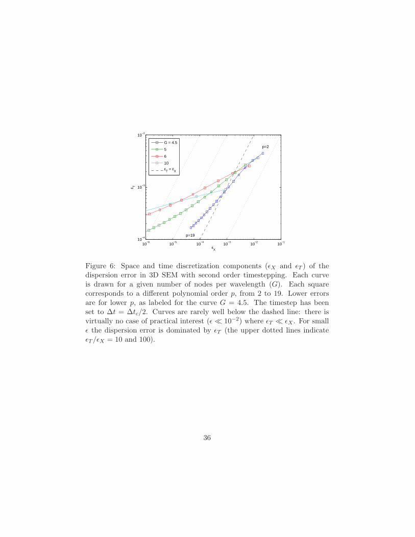
Figure 6: Space and time discretization components (ǫX and ǫT ) of thedispersion error in 3D SEM with second order timestepping. Each curveis drawn for a given number of nodes per wavelength (G). Each squarecorresponds to a different polynomial order p, from 2 to 19. Lower errorsare for lower p, as labeled for the curve G = 4.5. The timestep has beenset to ∆t = ∆tc/2. Curves are rarely well below the dashed line: there isvirtually no case of practical interest (ǫ≪ 10−2) where ǫT ≪ ǫX . For smallǫ the dispersion error is dominated by ǫT (the upper dotted lines indicateǫT /ǫX = 10 and 100).

36

4 nodes per wavelength are employed. At G = 10, ǫT is about six orders ofmagnitude larger than ǫX .In Figure 6 we illustrate, for D = 3, γ = 0.5 and a range of values of pand G, that in virtually no case of practical relevance (ǫ≪ 1%) is the timediscretization error ǫT neglectable with respect to the space discretizationerror ǫX . In simulations requiring reasonable accuracy ǫ < 10−3, with theusual setting γ . 1, the dispersion error is largely dominated bythe low order time discretization errors and the advantages ofspectral convergence of the SEM are wasted. In such situations ǫT

must be controlled by reducing the timestep ∆t. For instance, for p = 6,G = 6, to achieve an error of 1% of a period over a propagation distance of100 wavelengths (ǫ = 10−4) one needs to reduce ǫT by a factor of 10. Thisrequires a

√10 ≈ 3-fold reduction of ∆t and implies a ≈ 3-fold increase in

computational cost. We will see in later sections that a more efficient errorreduction can be achieved with higher order time schemes (q > 2).

5.2 Higher-order symplectic schemes

There are several methods to achieve higher order in time integration. Theso-called symplectic timestepping algorithms are very convenient.The update of displacement and velocity fields, d and v, from time t tot + ∆t is composed of a n-stage sub-stepping iteration. For k = 1 to n, do:

t ← t + ak ∆t (5.17)

d ← d + ak ∆t v (5.18)

v ← v + bk ∆t M−1[−Kd + f(t)] (5.19)

Then apply the closing stage:

t ← t + an+1 ∆t (5.20)

d ← d + an+1 ∆t v (5.21)

This family of algorithms requires n evaluations of internal forces Kd perglobal timestep. The implementation is remarkably simple, it takes a fewlines of coding to modify existing SEM solvers, and it does not requireadditional memory storage. Time-reversibility is guaranteed by imposingthe following symmetries on the coefficients: ak = an+2−k and bk = bn+1−k.The order q of the method depends on the number of stages n and on thecoefficients ak and bk. The cost increases linearly with n. These parameterscan be optimized to achieve high accuracy at low cost.

37

For instance, a good fourth order algorithm is the position extended Forest-Ruth-like (PEFRL) scheme:

a1 = a5 = ξ b1 = b4 = 1/2− λ

a2 = a4 = χ b2 = b3 = λ (5.22)

a3 = 1− 2(χ + ξ)

with

ξ = 0.1786178958448091

λ = −0.2123418310626054

χ = −0.06626458266981849

Its error coefficient is B = 1/12500 and its critical CFL number is C =2.97633.

6 Miscellaneous

6.1 Limitations of the SEM

• quad mesh is not that flexible, no automated meshing algorithms

• spectral convergence is lost in non-smooth problems (singularities, ma-terial boundaries within element)

• time schemes are usually low order, need improvement

6.2 Advanced topics

• Dynamic faulting boundary conditions

• Geometrically non-conforming meshes: mortar elements

• Preconditioners (Schwartz). Condition number prop to P 3/h2 in 2D,see Canuto 5.3.4. See also Canuto (5.3.5), Deville (4.5.1), Karniadakis(4.2)

• spectral discontinuous Galerking methods

• a posteriori errors and adaptivity

• SEM on triangles and tetrahedra

38

A References

Bernardi and Maday (2001), “Spectral, spectral element and mortar elementmethods”: mathematical analysisBoyd (200?), “Spectral elements” (chapter of book in progress):Gottlieb and Hesthaven, “Spectral methods for hyperbolic problems”: dual-ity between modal Legendre aproximation and nodal Lagrange interpolation(section 2), computational efficiency (section 7.4)van de Vosse and Minev (1996), “Spectral element methods: theory andapplications”: spectral, pseudo-spectral and spectral elements (sections 2.2and 2.3)Deville, Fischer and Mund (2002), “High-order methods for incompressiblefluid flow”:Canuto, “Spectral Methods: Evolution to Complex Geometries and Appli-cations to Fluid Dynamics”: Chapter 5

B Available software

available SEM codes: SPECFEM3D, SEM2DPACK, Gaspar, SPECULOOS,SEAMmeshing software: CUBIT, GiD, EMC2

39

C Homework problems

C.1 Love wave modes in a horizontally layered medium

Consider shear waves on an elastic medium made of two horizontal layers.The shallow layer is thinner (H1 = 400 m) and has lower shear wave speed(c1 = 1000 m/s) than the deeper one (H2 = 3600 m and c2 = 2000 m/s).Density is the same in both layers, ρ = 2000 kg/m3. The top surface (atz = 0) is stress-free (Neumann) and the bottom surface (at z = Z = 4000 m)is displacement-locked (Dirichlet).For a given frequency f (or angular frequency ω = 2πf), we focus on Lovewaves, i.e. surface waves with motion in the out-of-plane y direction, hor-izontal and perpendicular to the propagation direction x. We consider adisplacement field d of the following form

d(x, z, t) = u(z) exp(iωt− ikx)y (C.1)

We will look for the depth distribution of displacement u(z). The strongform of this problem is:Find the displacement profile u(z) and horizontal wavenumber k such that

−ω2ρ(z)u(z) + k2µ(z)u(z) − d

dz

(

µ(z)du

dz

)

= 0 (C.2)

with the following boundary conditions:

du

dz(z = 0) = 0 (C.3)

u(z = H1 + H2) = 0 (C.4)

and continuity of u and du/dz across the material interface.This is actually an eigenvalue problem. It has multiple solution pairs, ormodes (eigenvalues km and eigenfunctions um(z)). The modes are orderedby decreasing value of their km. The fundamental mode corresponds tom = 0 and the overtones to m > 0 .

1. Formulate the weak form of the problem

2. The SEM discretization of the eigenvalue problem is:

Find nodal displacements um and wavenumber km such that

[Kz − ω2M]um = −k2mKxum (C.5)

40

Write down the expression for the local matrices Me, Kex and Ke

z. Notethat the structure of Kx is similar to that of M, and that the bot-tom node (Dirichlet condition) must be removed from the unknowns.Consider two cases:

(a) the layer interface interface lies inside an element (case A)

(b) the interface coincides with an inter-element boundary (Case B)

3. Write a code that

(a) generates a 1D mesh in which each element can have a differentsize. For case A, the top two elements should have size h = 300 mand the others h = 850 m. For case B, h = 400 m in layer 1 andh = 900 m in layer 2.

(b) computes the SEM matrices for cases A and B. Let the poly-nomial degree P (the same for all elements) be a user specifiedparameter.

(c) finds the two eigenvalues of the discrete problem that have thesmallest algebraic value (−k2

0 and −k21), and the associated eigen-

vectors

(d) evaluates by GLL quadrature a measure of error defined as theintegral of the squared difference between the SEM solutions andtheir exact values (computed analytically, see below):

ǫ =

∫ Z

0(uSEM

m (z)− uexactm (z))2 dz (C.6)

4. Set P = 5 and f = 2.5 Hz. Compute the depth profile of displacementfor the fundamental Love mode and its first overtone for cases A andB and for at least three different meshes, each with twice as highresolution (smaller elements) as the previous one.

5. Plot displacement as a function of depth for both modes at the highestresolution, together with their exact values.

6. For cases A and B, plot in log-log scale the error ǫ as a function of theaverage value of element size h over the mesh. Discuss.

Resources:

• Matlab functions provided:

41

– GetGLL.m computes the GLL quadrature nodes, weights and thematrix of Lagrange derivatives H.

– love analytic.m computes the exact solution analytically

• Generalized eigenvalue problems of the form: find um and λm suchthat

Aum = λmBum, (C.7)

can be solved in Matlab with the function eigs. In particular the firsttwo modes are given by eigs(A,B,2,’SA’). Try to exploit the sparsestructure of the matrices.

C.2 Wave propagation and numerical dispersion

Consider the propagation of scalar waves in a 1D elastic medium of finitesize, x ∈ [0, L] with L = 10, and uniform properties (density ρ = 1, wavespeed c = 1). The boundary conditions are free stress at both ends. Considera point source located at x = L/2 with the following source time function:

f(t) = (2τ − 1) exp(−τ) where τ = (πf0(t− t0))2 (C.8)

a Ricker wavelet with dominant frequency f0 = 0.5 and delay t0 = 1.5/f0.

1. Write a code that solves this wave propagation problem with the SEM.Set P = 8 and h = 1. Consider two different time schemes: leapfrog(case A) and the PEFRL symplectic scheme defined in Equation 5.22(case B). Set the timestep ∆t = 0.85 min(∆x)/c for case A, and ∆t =1.25 min(∆x)/c for case B, where min(∆x) is the smallest distancebetween GLL nodes.

2. Compute the solution up to t = 40L/c. Plot the seismogram (displace-ment solution as a function of time) in the node located at x = 0.

3. You should see multiple reflected phases in the seismogram. Extractthe timing Tk of the displacement peaks of each phase. Plot Tk − T0

as a function of k for cases A and B.

4. Plot the dispersion error of the last reflected phase, defined as thedifference between Tk−T0 and the theoretical travel time of this wave.

5. Repeat the simulations now reducing the timestep ∆t by a factor 2,then a factor 4. Plot the travel time error as a function of ∆t for casesA and B. Discuss.

42