Embed Size (px)
Citation preview
1
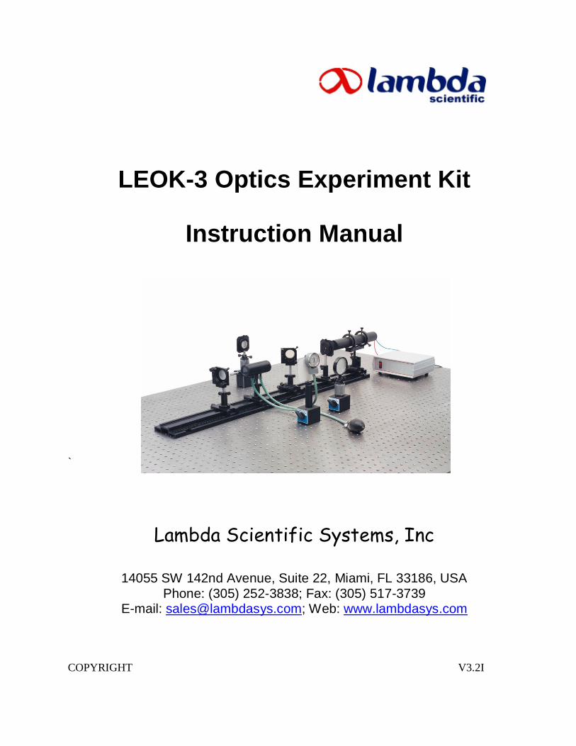
LEOK-3 Optics Experiment Kit
Instruction Manual
`
Lambda Scientific Systems, Inc
14055 SW 142nd Avenue, Suite 22, Miami, FL 33186, USA Phone: (305) 252-3838; Fax: (305) 517-3739
E-mail: [email protected]; Web: www.lambdasys.com
COPYRIGHT V3.2I
COMPANY PROFILE
Lambda Scientific Systems, Inc. specializes in developing and marketing scientific
instruments and systems designed and manufactured specifically for experimental
education in physics at colleges and universities. Our mission is to become a premier
supplier of high-quality, robust, easy-to-use, and affordable scientific instruments and
systems to college educators and students for their teaching and learning of both
fundamental and modern experiments in physics. Our products focus on comprehensive
physics education kits, as well as light sources and opto-mechanic components.
Our physics education kits cover a wide range of experiments in general physics,
especially in geometrical optics, physical optics, and fiber optics. Experiments include lens
imaging, interferometry, diffraction, holography, polarization, laser physics, quantum
optics, and Fourier optics through a series of the most representative apparatus such as
Newton’s ring apparatus, Young’s modulus apparatus, Michelson interferometer, Fabry-
Perot interferometer, Twyman-Green interferometer, Fourier spectrometer, and laser.
Our fiber optics education kits keep a pace with the advent of fiber optical communication
technology by designing experimental systems to teach fundamental optical fiber concepts
such as fiber-to-fiber coupling, fiber-to-source coupling, fiber numerical aperture, fiber
mode, fiber transmission loss, and fiber sensing. These kits also give students an
opportunity to be familiar with modern fiber optic components or apparatus such as Mach-
Zehnder interferometer, variable optical attenuator, fiber isolator, fiber splitter, fiber
switch, wavelength-division multiplexer, fiber amplifier, and transmitter.
Our light sources include Xenon lamp, Mercury lamp, Sodium lamp, Bromine Tungsten
lamp and various lasers.
We also provide a variety of opto-mechanical components such as optical mounts, optical
breadboards and translation stages. Our products have been sold worldwide. Lambda
Scientific Systems, Inc is committed to providing high quality, cost effective products and
on-time delivery.
CONTENTS
1. Introduction .............................................................................................................................1
2. Parts Included in the Kit ..........................................................................................................2
2.1 Light Sources ....................................................................................................................2
2.2 Mechanical Hardware ........................................................................................................2
2.3 Optical Components ..........................................................................................................5
2.4 Other Parts ........................................................................................................................6
2.5 Optional Parts ....................................................................................................................6
3. Experiment Examples..............................................................................................................7
3.1 Measuring the Focal Length of a Positive Thin Lens Using Auto-collimation ....................7
3.2 Measuring the Focal Length of a Positive Lens Using Displacement Method .....................9
3.3 Measuring the Focal Length of an Eyepiece..................................................................... 11
3.4 Assembling a Microscope ................................................................................................ 13
3.5 Assembling a Telescope .................................................................................................. 15
3.6 Assembling a Slide Projector ........................................................................................... 17
3.7 Measuring the Nodal Locations and Focal Lengths of a Lens-Group................................ 19
3.8 Assembling an Erect Imaging Telescope ......................................................................... 21
3.9 Young’s Double-Slit Interference .................................................................................... 23
3.10 Interference of Fresnel’s Biprism .................................................................................. 25
3.11 Interference of Double Mirrors ...................................................................................... 27
3.12 Interference of Lloyd’s Mirror ....................................................................................... 29
3.13 Interference of Newton’s Ring ....................................................................................... 31
3.14 Franhoffer Diffraction of a Single Silt............................................................................ 33
3.15 Franhoffer Diffraction of a Single Circular Aperture ...................................................... 35
3.16 Fresnel Diffraction of a Single Silt ................................................................................. 37
3.17 Fresnel Diffraction of a Single Circular Aperture ........................................................... 39
3.18 Fresnel Diffraction of a Sharp Edge ............................................................................... 41
3.19 Analysing Polarization Status of Light Beams ............................................................... 42
3.20 Diffraction of a Grating ................................................................................................. 45
3.21 Grating Monochromator ................................................................................................ 47
3.22 Recording and Reconstructing Holograms ..................................................................... 49
3.23 Making Holographic Gratings........................................................................................ 52
3.24 Abbe Imaging Principle and Optical Spatial Filtering .................................................... 54
3.25 Pseudo-Color Encoding, Theta Modulation and Color Composition .............................. 56
3.26 Assembling a Michelson Interferometer and Measuring the Refractive Index of Air ...... 58
4. Laser safety and lab requirements: ......................................................................................... 61
Appendix: User Instructions of Silver Salt Plates ................................................................... 61
1
1. Introduction
The LEOK-3 Optics Experiment Kit is developed for general physics education at universities and
colleges. This kit provides a complete set of optical and mechanical components as well as light
sources, which can be conveniently assembled to construct experimental setups. Almost all optics
experiments required in general physics education (e.g. geometrical, physical, and modern optics)
can be constructed in sequence using these components. Through selecting and assembling the
corresponding components into experimental setups, students can enhance their experimental skills
and problem solving ability.
LEOK-3 can be used to construct a total of 26 different experiments that can be grouped in six
categories:
Lens Measurements: Understanding and verifying lens equation and optical rays transform.
Optical Instruments: Understanding the working principle and operation method of common lab optical instruments.
Interference Phenomena: Understanding interference theory, observing various interference
patterns generated by different sources, and learning one precise measurement method based on optical interference.
Diffraction Phenomena: Understanding diffraction effects, observing various diffraction patterns generated by different apertures.
Analysis of Polarization: Understanding polarization and verifying polarization of light.
Fourier Optics and Holography: Understanding principles of advanced optics and their
applications.
List of experimental examples
Measuring the focal length of a positive thin lens using auto-collimation
Measuring the focal length of a positive thin lens using displacement method
Measuring the focal length of an eyepiece
Assembling a microscope
Assembling a telescope
Assembling a slide projector
Measuring the nodal locations and focal length of a lens-group
Assembling an erect imaging telescope
Young’s double-slit interference
Interference of Fresnel’s biprism
Interference of double mirrors
Interference of Lloyd’s mirror
Interference of Newton Ring
Fraunhofer diffraction of a single slit
Fraunhofer diffraction of a single circular aperture
Fresnel diffraction of a single slit
2
Fresnel diffraction of a single circular aperture
Fresnel diffraction of a sharp edge
Analysing polarization status of light beams
Diffraction of a grating
Assembling a Littrow-type grating spectrometer
Recording and reconstructing holograms
Fabricating a holographic grating
Abbe imaging principle and optical spatial filtering
Pseudo-color encoding, theta modulation and color composition
Assembling a Michelson interferometer and measuring the refractive index of air
2. Parts Included in the Kit
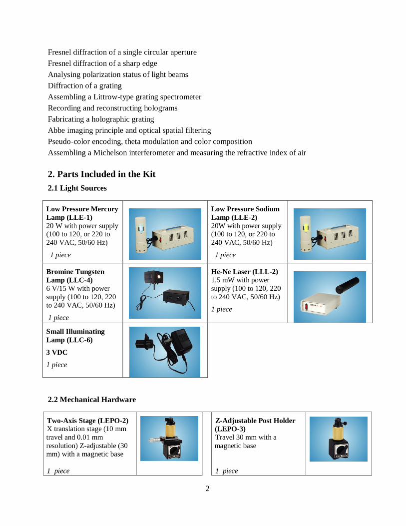
2.1 Light Sources
Low Pressure Mercury
Lamp (LLE-1)
20 W with power supply (100 to 120, or 220 to
240 VAC, 50/60 Hz)
1 piece
Low Pressure Sodium
Lamp (LLE-2)
20W with power supply (100 to 120, or 220 to
240 VAC, 50/60 Hz)
1 piece
Bromine Tungsten
Lamp (LLC-4)
6 V/15 W with power
supply (100 to 120, 220 to 240 VAC, 50/60 Hz)
1 piece
He-Ne Laser (LLL-2)
1.5 mW with power
supply (100 to 120, 220
to 240 VAC, 50/60 Hz)
1 piece
Small Illuminating
Lamp (LLC-6)
3 VDC
1 piece
2.2 Mechanical Hardware
Two-Axis Stage (LEPO-2) X translation stage (10 mm
travel and 0.01 mm
resolution) Z-adjustable (30 mm) with a magnetic base
1 piece
Z-Adjustable Post Holder
(LEPO-3)
Travel 30 mm with a
magnetic base
1 piece
3
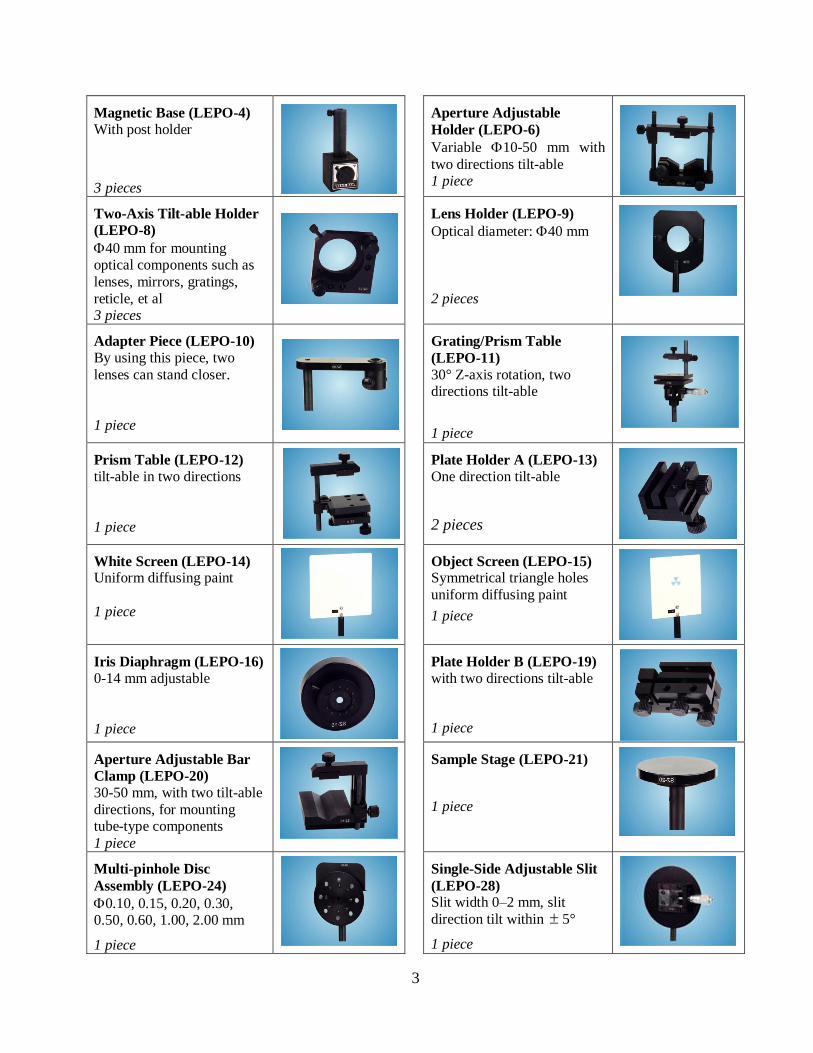
Magnetic Base (LEPO-4)
With post holder
3 pieces
Aperture Adjustable
Holder (LEPO-6)
Variable 10-50 mm with
two directions tilt-able 1 piece
Two-Axis Tilt-able Holder
(LEPO-8)
40 mm for mounting optical components such as
lenses, mirrors, gratings,
reticle, et al 3 pieces
Lens Holder (LEPO-9)
Optical diameter: 40 mm
2 pieces
Adapter Piece (LEPO-10)
By using this piece, two
lenses can stand closer.
1 piece
Grating/Prism Table
(LEPO-11)
30° Z-axis rotation, two directions tilt-able
1 piece
Prism Table (LEPO-12)
tilt-able in two directions
1 piece
Plate Holder A (LEPO-13)
One direction tilt-able
2 pieces
White Screen (LEPO-14) Uniform diffusing paint
1 piece
Object Screen (LEPO-15) Symmetrical triangle holes
uniform diffusing paint
1 piece
Iris Diaphragm (LEPO-16)
0-14 mm adjustable
1 piece
Plate Holder B (LEPO-19)
with two directions tilt-able
1 piece
Aperture Adjustable Bar
Clamp (LEPO-20)
30-50 mm, with two tilt-able
directions, for mounting tube-type components
1 piece
Sample Stage (LEPO-21)
1 piece
Multi-pinhole Disc
Assembly (LEPO-24)
0.10, 0.15, 0.20, 0.30, 0.50, 0.60, 1.00, 2.00 mm
1 piece
Single-Side Adjustable Slit
(LEPO-28) Slit width 0–2 mm, slit
direction tilt within 5°
1 piece
4
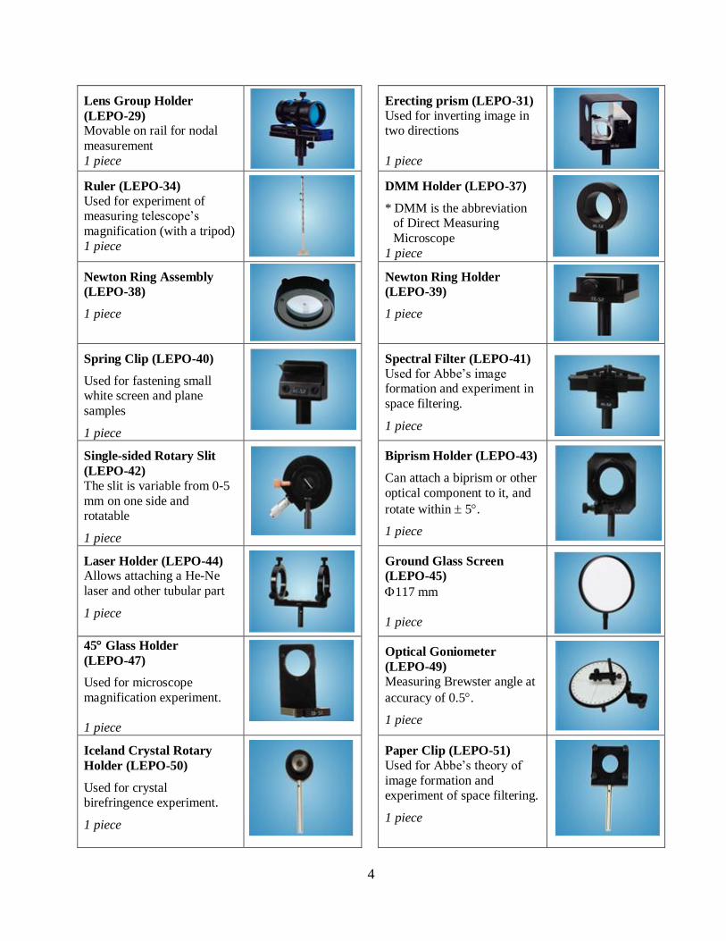
Lens Group Holder
(LEPO-29) Movable on rail for nodal
measurement
1 piece
Erecting prism (LEPO-31)
Used for inverting image in two directions
1 piece
Ruler (LEPO-34)
Used for experiment of measuring telescope’s
magnification (with a tripod)
1 piece
DMM Holder (LEPO-37)
* DMM is the abbreviation of Direct Measuring
Microscope
1 piece
Newton Ring Assembly
(LEPO-38)
1 piece
Newton Ring Holder
(LEPO-39)
1 piece
Spring Clip (LEPO-40)
Used for fastening small white screen and plane
samples
1 piece
Spectral Filter (LEPO-41)
Used for Abbe’s image formation and experiment in
space filtering.
1 piece
Single-sided Rotary Slit
(LEPO-42)
The slit is variable from 0-5
mm on one side and rotatable
1 piece
Biprism Holder (LEPO-43)
Can attach a biprism or other
optical component to it, and
rotate within 5.
1 piece
Laser Holder (LEPO-44) Allows attaching a He-Ne
laser and other tubular part
1 piece
Ground Glass Screen
(LEPO-45)
117 mm
1 piece
45 Glass Holder
(LEPO-47)
Used for microscope
magnification experiment.
1 piece
Optical Goniometer
(LEPO-49)
Measuring Brewster angle at
accuracy of 0.5.
1 piece
Iceland Crystal Rotary
Holder (LEPO-50)
Used for crystal birefringence experiment.
1 piece
Paper Clip (LEPO-51)
Used for Abbe’s theory of
image formation and experiment of space filtering.
1 piece
5
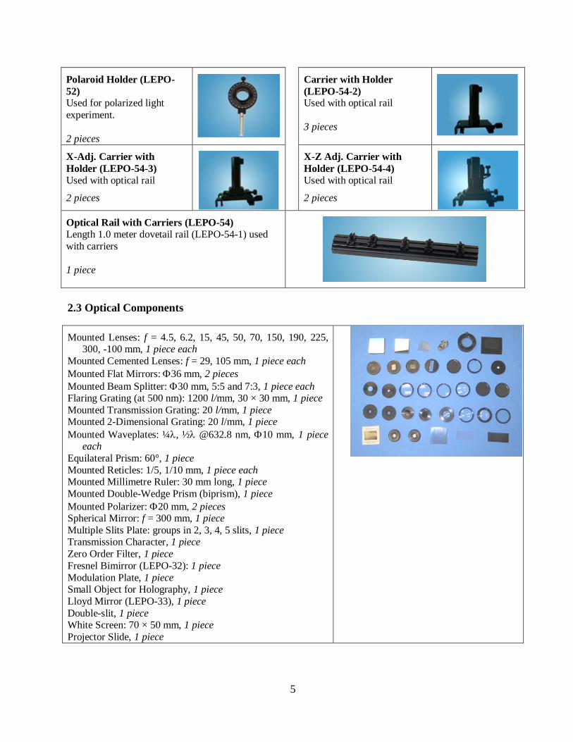
Polaroid Holder (LEPO-
52) Used for polarized light
experiment.
2 pieces
Carrier with Holder
(LEPO-54-2) Used with optical rail
3 pieces
X-Adj. Carrier with
Holder (LEPO-54-3)
Used with optical rail
2 pieces
X-Z Adj. Carrier with
Holder (LEPO-54-4)
Used with optical rail
2 pieces
Optical Rail with Carriers (LEPO-54)
Length 1.0 meter dovetail rail (LEPO-54-1) used
with carriers
1 piece
2.3 Optical Components
Mounted Lenses: f = 4.5, 6.2, 15, 45, 50, 70, 150, 190, 225, 300, -100 mm, 1 piece each
Mounted Cemented Lenses: f = 29, 105 mm, 1 piece each
Mounted Flat Mirrors: 36 mm, 2 pieces
Mounted Beam Splitter: 30 mm, 5:5 and 7:3, 1 piece each Flaring Grating (at 500 nm): 1200 l/mm, 30 × 30 mm, 1 piece
Mounted Transmission Grating: 20 l/mm, 1 piece Mounted 2-Dimensional Grating: 20 l/mm, 1 piece
Mounted Waveplates: ¼, ½ @632.8 nm, 10 mm, 1 piece each
Equilateral Prism: 60°, 1 piece
Mounted Reticles: 1/5, 1/10 mm, 1 piece each Mounted Millimetre Ruler: 30 mm long, 1 piece
Mounted Double-Wedge Prism (biprism), 1 piece
Mounted Polarizer: 20 mm, 2 pieces Spherical Mirror: f = 300 mm, 1 piece
Multiple Slits Plate: groups in 2, 3, 4, 5 slits, 1 piece Transmission Character, 1 piece
Zero Order Filter, 1 piece
Fresnel Bimirror (LEPO-32): 1 piece
Modulation Plate, 1 piece Small Object for Holography, 1 piece
Lloyd Mirror (LEPO-33), 1 piece
Double-slit, 1 piece White Screen: 70 × 50 mm, 1 piece
Projector Slide, 1 piece
6
2.4 Other Parts
Description Part No. Qty Note
Holographic Plate GS-I 1 Box 12 pcs, 9×24 cm each, glass
530 700 nm, peak @630 nm
Air Chamber and Pump with
Gauge
LEPO-55 1 3 40 kpa/20 300 mm Hg
used for air index measurement
Direct Measurement Microscope LEPO-56 1 20×
2.5 Optional Parts
Description Part No. Qty Note
Parts Holder Stand LEPO-57 1 each stand can hold 20 parts
* Note: Above parts are subject to change without notice.
7
3. Experiment Examples
3.1 Measuring the Focal Length of a Positive Thin Lens Using Auto-collimation
Objective:
Understand the principle and method of measuring the focal length of a lens using auto-collimation.
Experimental Setup
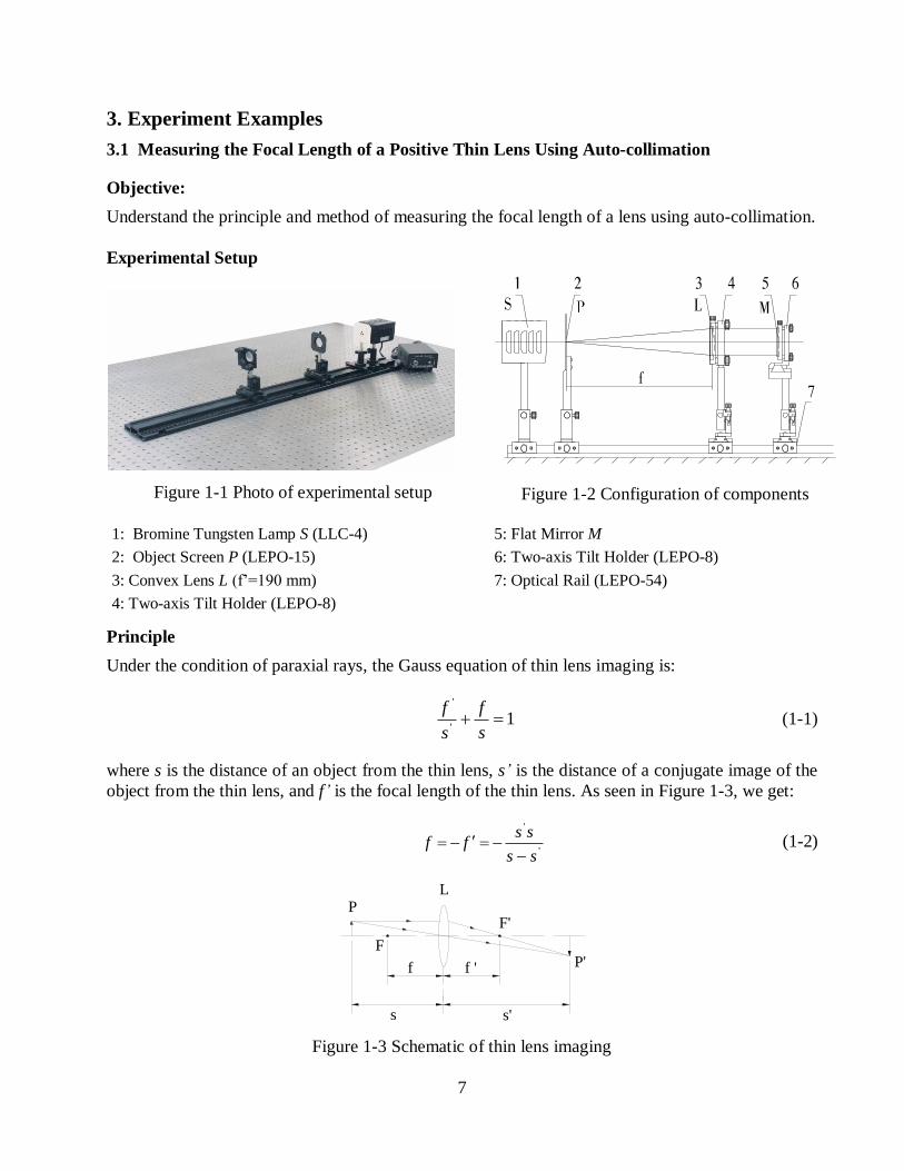
Figure 1-1 Photo of experimental setup
Figure 1-2 Configuration of components
1: Bromine Tungsten Lamp S (LLC-4)
2: Object Screen P (LEPO-15)
3: Convex Lens L (f’=190 mm)
4: Two-axis Tilt Holder (LEPO-8)
5: Flat Mirror M
6: Two-axis Tilt Holder (LEPO-8)
7: Optical Rail (LEPO-54)
Principle
Under the condition of paraxial rays, the Gauss equation of thin lens imaging is:
1'
'
s
f
s
f (1-1)
where s is the distance of an object from the thin lens, s’ is the distance of a conjugate image of the
object from the thin lens, and f’ is the focal length of the thin lens. As seen in Figure 1-3, we get:
'
'
ss
ssff
(1-2)
s's
f 'f
L
F'
FP'
P
Figure 1-3 Schematic of thin lens imaging
8
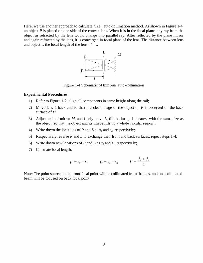
Here, we use another approach to calculate f, i.e., auto-collimation method. As shown in Figure 1-4,
an object P is placed on one side of the convex lens. When it is in the focal plane, any ray from the
object as refracted by the lens would change into parallel ray. After reflected by the plane mirror
and again refracted by the lens, it is converged in focal plane of the lens. The distance between lens
and object is the focal length of the lens: f = s
Figure 1-4 Schematic of thin lens auto-collimation
Experimental Procedures:
1) Refer to Figure 1-2, align all components in same height along the rail;
2) Move lens L back and forth, till a clear image of the object on P is observed on the back
surface of P;
3) Adjust axis of mirror M, and finely move L, till the image is clearest with the same size as
the object (so that the object and its image fills up a whole circular region);
4) Write down the locations of P and L as s1 and s2, respectively;
5) Respectively reverse P and L to exchange their front and back surfaces, repeat steps 1-4;
6) Write down new locations of P and L as s3 and s4, respectively;
7) Calculate focal length:
12
,
1 ssf 34
,
2 ssf 2
,
2
,
1, fff
Note: The point source on the front focal point will be collimated from the lens, and one collimated
beam will be focused on back focal point.
P’
M P
L
s
9
3.2 Measuring the Focal Length of a Positive Lens Using Displacement Method
Objective:
Understand the principle and method for measuring the focal length of a lens with displacement
approach, and verify “lens equation”
Experimental Setup
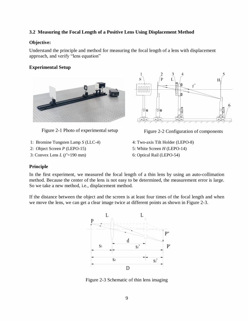
Figure 2-1 Photo of experimental setup
Figure 2-2 Configuration of components
1: Bromine Tungsten Lamp S (LLC-4)
2: Object Screen P (LEPO-15)
3: Convex Lens L (f’=190 mm)
4: Two-axis Tilt Holder (LEPO-8)
5: White Screen H (LEPO-14)
6: Optical Rail (LEPO-54)
Principle
In the first experiment, we measured the focal length of a thin lens by using an auto-collimation
method. Because the center of the lens is not easy to be determined, the measurement error is large.
So we take a new method, i.e., displacement method.
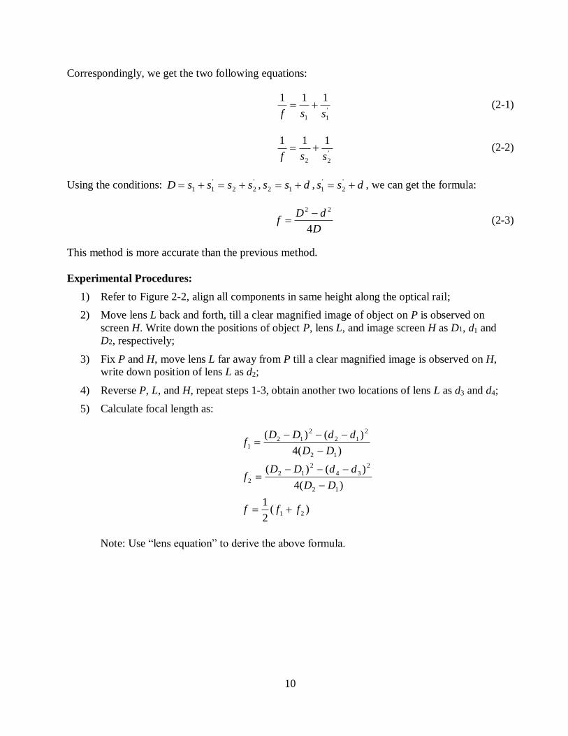
If the distance between the object and the screen is at least four times of the focal length and when
we move the lens, we can get a clear image twice at different points as shown in Figure 2-3.
D
d
P''
s2's2
s1'
L
P'
PL
s1
Figure 2-3 Schematic of thin lens imaging
10
Correspondingly, we get the two following equations:
'
11
111
ssf (2-1)
'
22
111
ssf (2-2)
Using the conditions: '
22
'
11 ssssD , dss 12 , dss '
2
'
1 , we can get the formula:
D
dDf
4
22 (2-3)
This method is more accurate than the previous method.
Experimental Procedures:
1) Refer to Figure 2-2, align all components in same height along the optical rail;
2) Move lens L back and forth, till a clear magnified image of object on P is observed on
screen H. Write down the positions of object P, lens L, and image screen H as D1, d1 and
D2, respectively;
3) Fix P and H, move lens L far away from P till a clear magnified image is observed on H,
write down position of lens L as d2;
4) Reverse P, L, and H, repeat steps 1-3, obtain another two locations of lens L as d3 and d4;
5) Calculate focal length as:
)(2
1
)(4
)()(
)(4
)()(
21
12
2
34
2
12
2
12
2
12
2
121
fff
DD
ddDDf
DD
ddDDf
Note: Use “lens equation” to derive the above formula.
11
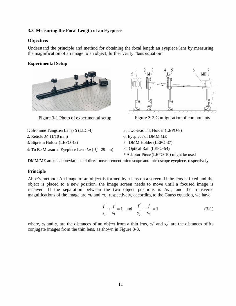
3.3 Measuring the Focal Length of an Eyepiece
Objective:
Understand the principle and method for obtaining the focal length an eyepiece lens by measuring
the magnification of an image to an object; further verify “lens equation”
Experimental Setup
Figure 3-1 Photo of experimental setup
Figure 3-2 Configuration of components
1: Bromine Tungsten Lamp S (LLC-4)
2: Reticle M (1/10 mm)
3: Biprism Holder (LEPO-43)
4: To Be Measured Eyepiece Lens Le (,
ef =29mm)
5: Two-axis Tilt Holder (LEPO-8)
6: Eyepiece of DMM ME
7: DMM Holder (LEPO-37)
8: Optical Rail (LEPO-54)
* Adaptor Piece (LEPO-10) might be used
DMM/ME are the abbreviations of direct measurement microscope and microscope eyepiece, respectively
Principle
Abbe’s method: An image of an object is formed by a lens on a screen. If the lens is fixed and the
object is placed to a new position, the image screen needs to move until a focused image is
received. If the separation between the two object positions is s , and the transverse
magnifications of the image are m1 and m2, respectively, according to the Gauss equation, we have:
11
'
1
'
s
f
s
f and 1
2
'
2
'
s
f
s
f (3-1)
where, s1 and s2 are the distances of an object from a thin lens, s1’ and s2’ are the distances of its
conjugate images from the thin lens, as shown in Figure 3-3.
12
s2's2
s1's1 y2
y1
y
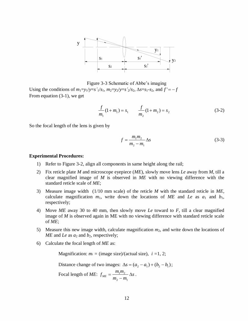
Figure 3-3 Schematic of Abbe’s imaging
Using the conditions of m1=y1/y=s’1/s1, m2=y2/y=s’2/s2, s=s1-s2, and ff '
From equation (3-1), we get
11
1
)1( smm
f 22
2
)1( smm
f (3-2)
So the focal length of the lens is given by
smm
mmf
12
21 (3-3)
Experimental Procedures:
1) Refer to Figure 3-2, align all components in same height along the rail;
2) Fix reticle plate M and microscope eyepiece (ME), slowly move lens Le away from M, till a
clear magnified image of M is observed in ME with no viewing difference with the
standard reticle scale of ME;
3) Measure image width (1/10 mm scale) of the reticle M with the standard reticle in ME,
calculate magnification m1, write down the locations of ME and Le as a1 and b1,
respectively;
4) Move ME away 30 to 40 mm, then slowly move Le toward to F, till a clear magnified
image of M is observed again in ME with no viewing difference with standard reticle scale
of ME;
5) Measure this new image width, calculate magnification m2, and write down the locations of
ME and Le as a2 and b2, respectively;
6) Calculate the focal length of ME as:
Magnification: mi = (image size)/(actual size), i =1, 2;
Distance change of two images: )()( 1212 bbaas ;
Focal length of ME: smm
mmfME
12
21 .
13
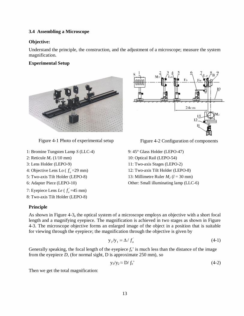
3.4 Assembling a Microscope
Objective:
Understand the principle, the construction, and the adjustment of a microscope; measure the system
magnification.
Experimental Setup
Figure 4-1 Photo of experimental setup
Figure 4-2 Configuration of components
1: Bromine Tungsten Lamp S (LLC-4)
2: Reticule M1 (1/10 mm)
3: Lens Holder (LEPO-9)
4: Objective Lens Lo ('
of =29 mm)
5: Two-axis Tilt Holder (LEPO-8)
6: Adapter Piece (LEPO-10)
7: Eyepiece Lens Le ('
ef =45 mm)
8: Two-axis Tilt Holder (LEPO-8)
9: 45° Glass Holder (LEPO-47)
10: Optical Rail (LEPO-54)
11: Two-axis Stages (LEPO-2)
12: Two-axis Tilt Holder (LEPO-8)
13: Millimetre Ruler M2 (l = 30 mm)
Other: Small illuminating lamp (LLC-6)
Principle
As shown in Figure 4-3, the optical system of a microscope employs an objective with a short focal
length and a magnifying eyepiece. The magnification is achieved in two stages as shown in Figure
4-3. The microscope objective forms an enlarged image of the object in a position that is suitable
for viewing through the eyepiece; the magnification through the objective is given by
'
12 //yy of (4-1)
Generally speaking, the focal length of the eyepiece fe’ is much less than the distance of the image
from the eyepiece D, (for normal sight, D is approximate 250 mm), so
y3/y2 ≈ D/ fe’ (4-2)
Then we get the total magnification:
14
''
1
2
2
3
1
3
eo ff
D
y
y
y
y
y
yM
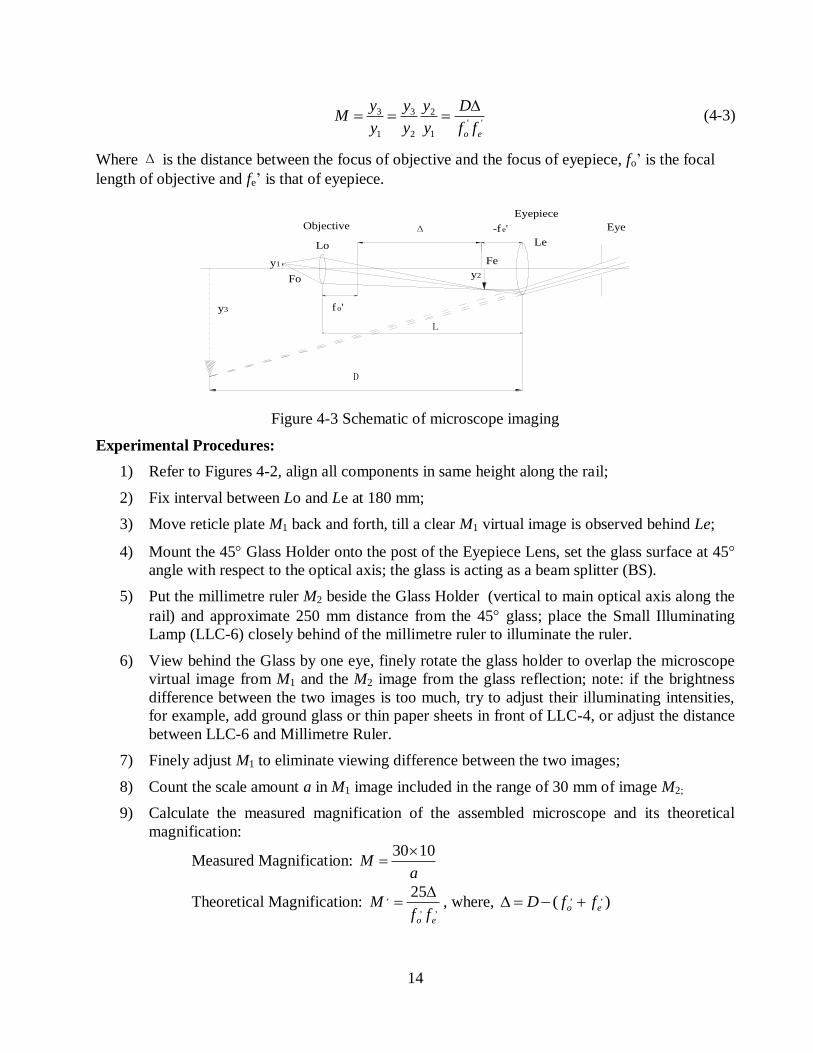
(4-3)
Where Δ is the distance between the focus of objective and the focus of eyepiece, fo’ is the focal
length of objective and fe’ is that of eyepiece.
Figure 4-2
y3
y2
y1
D
-f e'
fo'
L
Lo
Fo
Le
Fe
Δ Eye
Eyepiece
Objective
Figure 4-3 Schematic of microscope imaging
Experimental Procedures:
1) Refer to Figures 4-2, align all components in same height along the rail;
2) Fix interval between Lo and Le at 180 mm;
3) Move reticle plate M1 back and forth, till a clear M1 virtual image is observed behind Le;
4) Mount the 45 Glass Holder onto the post of the Eyepiece Lens, set the glass surface at 45
angle with respect to the optical axis; the glass is acting as a beam splitter (BS).
5) Put the millimetre ruler M2 beside the Glass Holder (vertical to main optical axis along the
rail) and approximate 250 mm distance from the 45 glass; place the Small Illuminating
Lamp (LLC-6) closely behind of the millimetre ruler to illuminate the ruler.
6) View behind the Glass by one eye, finely rotate the glass holder to overlap the microscope
virtual image from M1 and the M2 image from the glass reflection; note: if the brightness
difference between the two images is too much, try to adjust their illuminating intensities,
for example, add ground glass or thin paper sheets in front of LLC-4, or adjust the distance
between LLC-6 and Millimetre Ruler.
7) Finely adjust M1 to eliminate viewing difference between the two images;
8) Count the scale amount a in M1 image included in the range of 30 mm of image M2;
9) Calculate the measured magnification of the assembled microscope and its theoretical
magnification:
Measured Magnification: a
M1030
Theoretical Magnification: ,,
, 25
eo ffM
, where, )( ,,
eo ffD
15
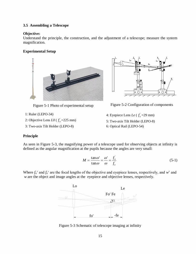
3.5 Assembling a Telescope
Objective:
Understand the principle, the construction, and the adjustment of a telescope; measure the system
magnification.
Experimental Setup
Figure 5-1 Photo of experimental setup
Figure 5-2 Configuration of components
1: Ruler (LEPO-34)
2: Objective Lens L0 ('
of =225 mm)
3: Two-axis Tilt Holder (LEPO-8)
4: Eyepiece Lens Le ('
ef =29 mm)
5: Two-axis Tilt Holder (LEPO-8)
6: Optical Rail (LEPO-54)
Principle
As seen in Figure 5-3, the magnifying power of a telescope used for observing objects at infinity is
defined as the angular magnification at the pupils because the angles are very small:
'
''
tan
'tan
e
o
f
fM
(5-1)
Where fo‘ and fe‘ are the focal lengths of the objective and eyepiece lenses, respectively, and w’ and
w are the object and image angles at the eyepiece and objective lenses, respectively.
y2
-fefo'
Fo' Fe
LeLo
Figure 5-3 Schematic of telescope imaging at infinity
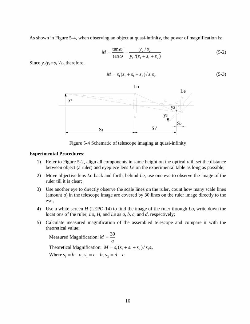
16
As shown in Figure 5-4, when observing an object at quasi-infinity, the power of magnification is:
)/(
/
tan
'tan
2
'
111
22
sssy
syM
(5-2)
Since y2/y1=s1’/s1, therefore,
212
'
11
'
1 /)( ssssssM (5-3)
S2
S1'
LeLo
y1
y3
y2
S1
Figure 5-4 Schematic of telescope imaging at quasi-infinity
Experimental Procedures:
1) Refer to Figure 5-2, align all components in same height on the optical rail, set the distance
between object (a ruler) and eyepiece lens Le on the experimental table as long as possible;
2) Move objective lens Lo back and forth, behind Le, use one eye to observe the image of the
ruler till it is clear;
3) Use another eye to directly observe the scale lines on the ruler, count how many scale lines
(amount a) in the telescope image are covered by 30 lines on the ruler image directly to the
eye;
4) Use a white screen H (LEPO-14) to find the image of the ruler through Lo, write down the
locations of the ruler, Lo, H, and Le as a, b, c, and d, respectively;
5) Calculate measured magnification of the assembled telescope and compare it with the
theoretical value:
Measured Magnification:a
M30
Theoretical Magnification: 212
'
11
'
1 /)( ssssssM
Where abs 1 , bcs '
1 , cds 2
17
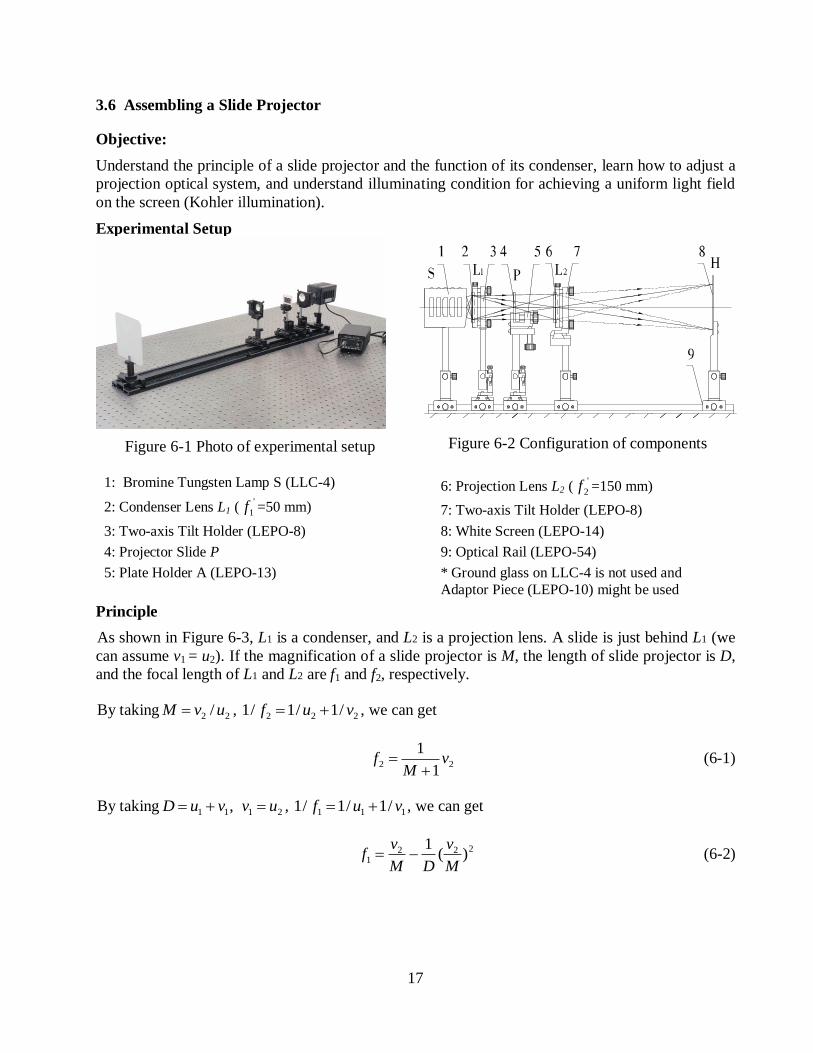
3.6 Assembling a Slide Projector
Objective:
Understand the principle of a slide projector and the function of its condenser, learn how to adjust a
projection optical system, and understand illuminating condition for achieving a uniform light field
on the screen (Kohler illumination).
Experimental Setup
Figure 6-1 Photo of experimental setup
Figure 6-2 Configuration of components
1: Bromine Tungsten Lamp S (LLC-4)
2: Condenser Lens L1 ('
1f =50 mm)
3: Two-axis Tilt Holder (LEPO-8)
4: Projector Slide P
5: Plate Holder A (LEPO-13)
6: Projection Lens L2 ('
2f =150 mm)
7: Two-axis Tilt Holder (LEPO-8)
8: White Screen (LEPO-14)
9: Optical Rail (LEPO-54)
* Ground glass on LLC-4 is not used and
Adaptor Piece (LEPO-10) might be used
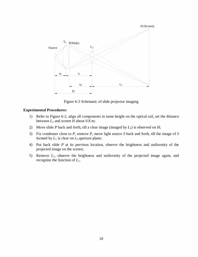
Principle
As shown in Figure 6-3, L1 is a condenser, and L2 is a projection lens. A slide is just behind L1 (we
can assume v1 = u2). If the magnification of a slide projector is M, the length of slide projector is D,
and the focal length of L1 and L2 are f1 and f2, respectively.
By taking 22 /uvM , 222 /1/1/1 vuf , we can get
221
1v
Mf
(6-1)
By taking ,11 vuD 21 uv , 111 /1/1/1 vuf , we can get
2221 )(
1
M
v
DM
vf (6-2)
18
D
H (Screen)
L2
P(Slide)L1
Source
v2u2
v1u1
Figure 6-3 Schematic of slide projector imaging
Experimental Procedures:
1) Refer to Figure 6-2, align all components in same height on the optical rail, set the distance
between L2 and screen H about 0.8 m;
2) Move slide P back and forth, till a clear image (imaged by L2) is observed on H;
3) Fix condenser close to P, remove P, move light source S back and forth, till the image of S
formed by L1 is clear on L2 aperture plane;
4) Put back slide P at its pervious location, observe the brightness and uniformity of the
projected image on the screen;
5) Remove L1, observe the brightness and uniformity of the projected image again, and
recognize the function of L1.
19
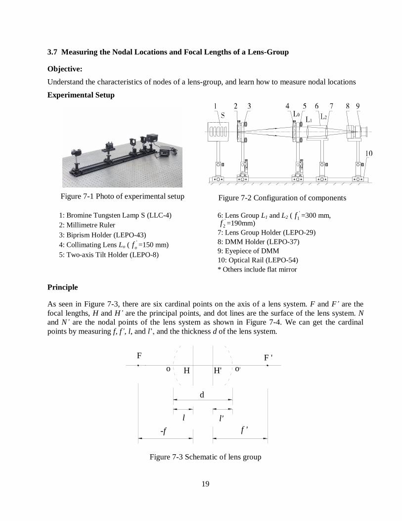
3.7 Measuring the Nodal Locations and Focal Lengths of a Lens-Group
Objective:
Understand the characteristics of nodes of a lens-group, and learn how to measure nodal locations
Experimental Setup
Figure 7-1 Photo of experimental setup
Figure 7-2 Configuration of components
1: Bromine Tungsten Lamp S (LLC-4)
2: Millimetre Ruler
3: Biprism Holder (LEPO-43)
4: Collimating Lens Lo ('
of =150 mm)
5: Two-axis Tilt Holder (LEPO-8)
6: Lens Group L1 and L2 ('
1f =300 mm, '
2f =190mm)
7: Lens Group Holder (LEPO-29)
8: DMM Holder (LEPO-37)
9: Eyepiece of DMM
10: Optical Rail (LEPO-54)
* Others include flat mirror
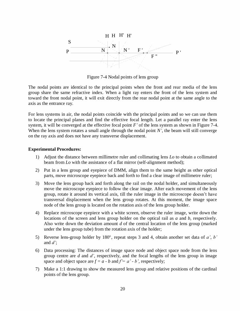
Principle
As seen in Figure 7-3, there are six cardinal points on the axis of a lens system. F and F’ are the
focal lengths, H and H’ are the principal points, and dot lines are the surface of the lens system. N
and N’ are the nodal points of the lens system as shown in Figure 7-4. We can get the cardinal
points by measuring f, f’, l, and l’, and the thickness d of the lens system.
f ' -f
H'H
l'l
d
o'
F '
o
F
Figure 7-3 Schematic of lens group
20
N 'P 'P
SN
N
H'H'HH
F ''
F '
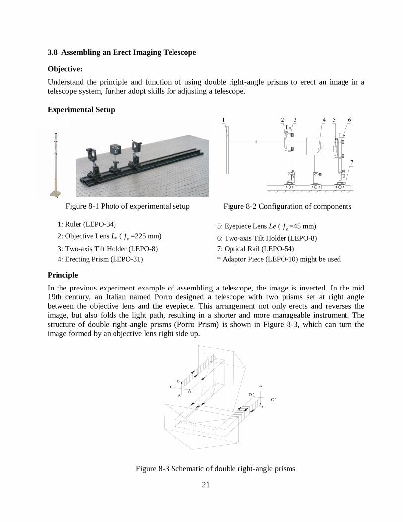
Figure 7-4 Nodal points of lens group
The nodal points are identical to the principal points when the front and rear media of the lens
group share the same refractive index. When a light ray enters the front of the lens system and
toward the front nodal point, it will exit directly from the rear nodal point at the same angle to the
axis as the entrance ray.
For lens systems in air, the nodal points coincide with the principal points and so we can use them
to locate the principal planes and find the effective focal length. Let a parallel ray enter the lens
system, it will be converged at the effective focal point F’ of the lens system as shown in Figure 7-4.
When the lens system rotates a small angle through the nodal point N’, the beam will still converge
on the ray axis and does not have any transverse displacement.
Experimental Procedures:
1) Adjust the distance between millimetre ruler and collimating lens Lo to obtain a collimated
beam from Lo with the assistance of a flat mirror (self-alignment method);
2) Put in a lens group and eyepiece of DMM, align them to the same height as other optical
parts, move microscope eyepiece back and forth to find a clear image of millimetre ruler;
3) Move the lens group back and forth along the rail on the nodal holder, and simultaneously
move the microscope eyepiece to follow the clear image. After each movement of the lens
group, rotate it around its vertical axis, till the ruler image in the microscope doesn’t have
transversal displacement when the lens group rotates. At this moment, the image space
node of the lens group is located on the rotation axis of the lens group holder.
4) Replace microscope eyepiece with a white screen, observe the ruler image, write down the
locations of the screen and lens group holder on the optical rail as a and b, respectively.
Also write down the deviation amount d of the central location of the lens group (marked
under the lens group tube) from the rotation axis of the holder;
5) Reverse lens-group holder by 180, repeat steps 3 and 4, obtain another set data of a’, b’
and d’;
6) Data processing: The distances of image space node and object space node from the lens
group centre are d and d’, respectively, and the focal lengths of the lens group in image
space and object space are f = a - b and f’= a’ - b’, respectively;
7) Make a 1:1 drawing to show the measured lens group and relative positions of the cardinal
points of the lens group.
21
3.8 Assembling an Erect Imaging Telescope
Objective:
Understand the principle and function of using double right-angle prisms to erect an image in a
telescope system, further adopt skills for adjusting a telescope.
Experimental Setup
Figure 8-1 Photo of experimental setup
Figure 8-2 Configuration of components
1: Ruler (LEPO-34)
2: Objective Lens Lo ('
of =225 mm)
3: Two-axis Tilt Holder (LEPO-8)
4: Erecting Prism (LEPO-31)
5: Eyepiece Lens Le ('
ef =45 mm)
6: Two-axis Tilt Holder (LEPO-8)
7: Optical Rail (LEPO-54)
* Adaptor Piece (LEPO-10) might be used
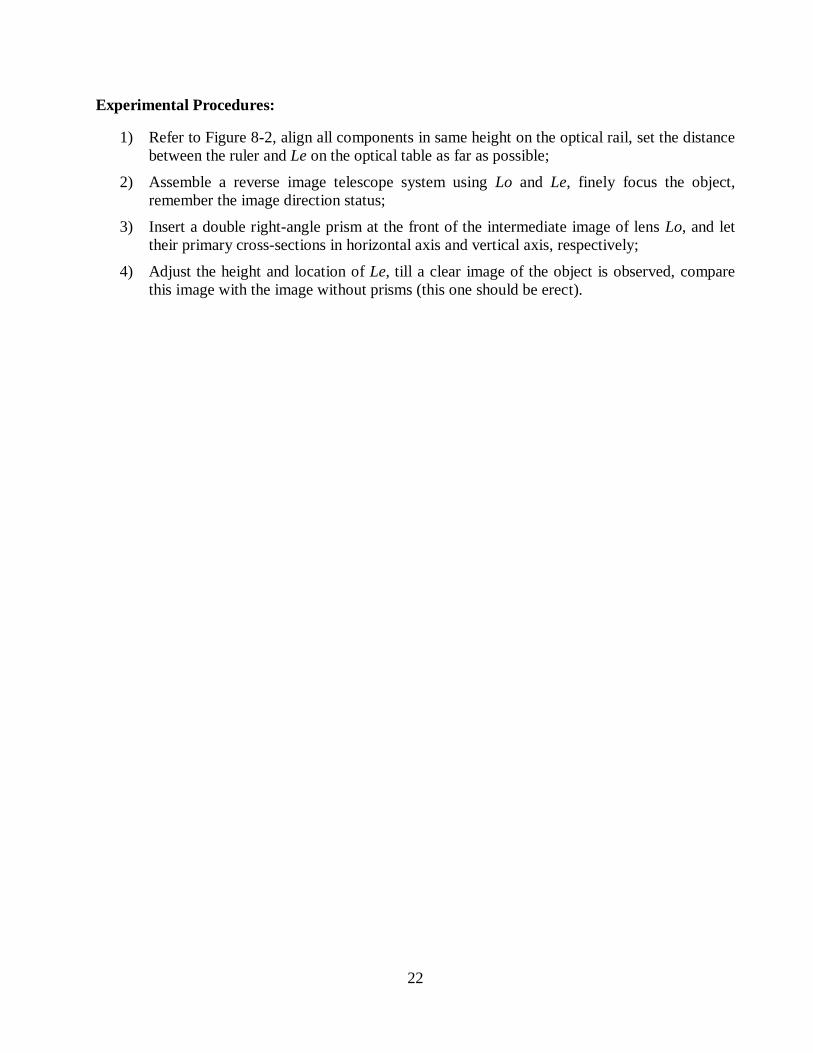
Principle
In the previous experiment example of assembling a telescope, the image is inverted. In the mid
19th century, an Italian named Porro designed a telescope with two prisms set at right angle
between the objective lens and the eyepiece. This arrangement not only erects and reverses the
image, but also folds the light path, resulting in a shorter and more manageable instrument. The
structure of double right-angle prisms (Porro Prism) is shown in Figure 8-3, which can turn the
image formed by an objective lens right side up.
D '
C '
B '
A '
D
C
B
A
Figure 8-3 Schematic of double right-angle prisms
22
Experimental Procedures:
1) Refer to Figure 8-2, align all components in same height on the optical rail, set the distance
between the ruler and Le on the optical table as far as possible;
2) Assemble a reverse image telescope system using Lo and Le, finely focus the object,
remember the image direction status;
3) Insert a double right-angle prism at the front of the intermediate image of lens Lo, and let
their primary cross-sections in horizontal axis and vertical axis, respectively;
4) Adjust the height and location of Le, till a clear image of the object is observed, compare
this image with the image without prisms (this one should be erect).
23
3.9 Young’s Double-Slit Interference
Objective:
Observe Young’s double-slit interference phenomena and measure the wavelength of light.
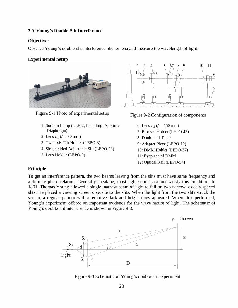
Experimental Setup
Figure 9-1 Photo of experimental setup
Figure 9-2 Configuration of components
1: Sodium Lamp (LLE-2, including Aperture
Diaphragm)
2: Lens L1 (f’= 50 mm)
3: Two-axis Tilt Holder (LEPO-8)
4: Single-sided Adjustable Slit (LEPO-28)
5: Lens Holder (LEPO-9)
6: Lens L2 (f’= 150 mm)
7: Biprism Holder (LEPO-43)
8: Double-slit Plate
9: Adapter Piece (LEPO-10)
10: DMM Holder (LEPO-37)
11: Eyepiece of DMM
12: Optical Rail (LEPO-54)
Principle
To get an interference pattern, the two beams leaving from the slits must have same frequency and
a definite phase relation. Generally speaking, most light sources cannot satisfy this condition. In
1801, Thomas Young allowed a single, narrow beam of light to fall on two narrow, closely spaced
slits. He placed a viewing screen opposite to the slits. When the light from the two slits struck the
screen, a regular pattern with alternative dark and bright rings appeared. When first performed,
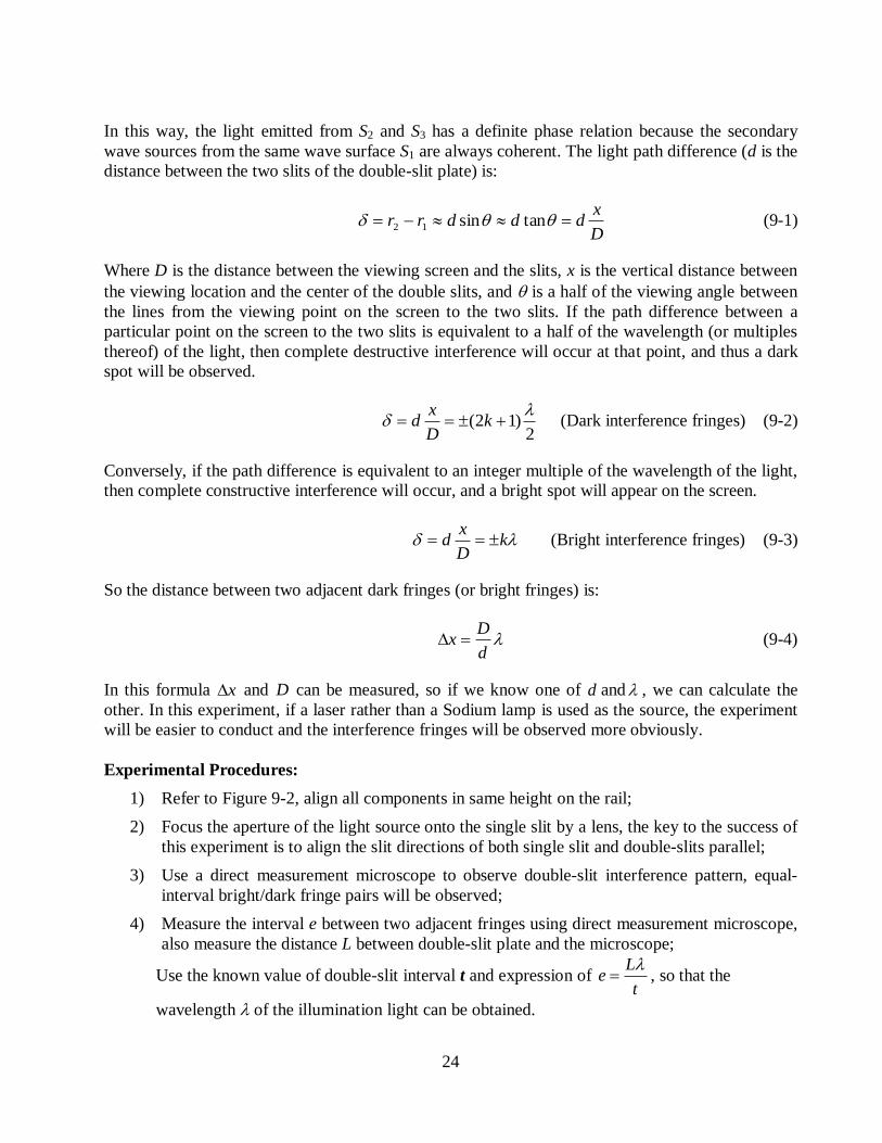
Young’s experiment offered an important evidence for the wave nature of light. The schematic of
Young’s double-slit interference is shown in Figure 9-3.
Lightδ
θ
D
x
ScreenP
r2
r1
d
S3
S2
S1
Figure 9-3 Schematic of Young’s double-slit experiment
24
In this way, the light emitted from S2 and S3 has a definite phase relation because the secondary
wave sources from the same wave surface S1 are always coherent. The light path difference (d is the
distance between the two slits of the double-slit plate) is:
D
xdddrr tansin12 (9-1)
Where D is the distance between the viewing screen and the slits, x is the vertical distance between
the viewing location and the center of the double slits, and is a half of the viewing angle between
the lines from the viewing point on the screen to the two slits. If the path difference between a
particular point on the screen to the two slits is equivalent to a half of the wavelength (or multiples
thereof) of the light, then complete destructive interference will occur at that point, and thus a dark
spot will be observed.
2)12(
kD
xd (Dark interference fringes) (9-2)
Conversely, if the path difference is equivalent to an integer multiple of the wavelength of the light,
then complete constructive interference will occur, and a bright spot will appear on the screen.
kD
xd (Bright interference fringes) (9-3)
So the distance between two adjacent dark fringes (or bright fringes) is:
d
Dx (9-4)
In this formula x and D can be measured, so if we know one of d and , we can calculate the
other. In this experiment, if a laser rather than a Sodium lamp is used as the source, the experiment
will be easier to conduct and the interference fringes will be observed more obviously.
Experimental Procedures:
1) Refer to Figure 9-2, align all components in same height on the rail;
2) Focus the aperture of the light source onto the single slit by a lens, the key to the success of
this experiment is to align the slit directions of both single slit and double-slits parallel;
3) Use a direct measurement microscope to observe double-slit interference pattern, equal-
interval bright/dark fringe pairs will be observed;
4) Measure the interval e between two adjacent fringes using direct measurement microscope,
also measure the distance L between double-slit plate and the microscope;
Use the known value of double-slit interval t and expression of t
Le
, so that the
wavelength of the illumination light can be obtained.
25
3.10 Interference of Fresnel’s Biprism
Objective:
Observe Fresnel’s bi-prism interference phenomena and measure the wavelength of light.
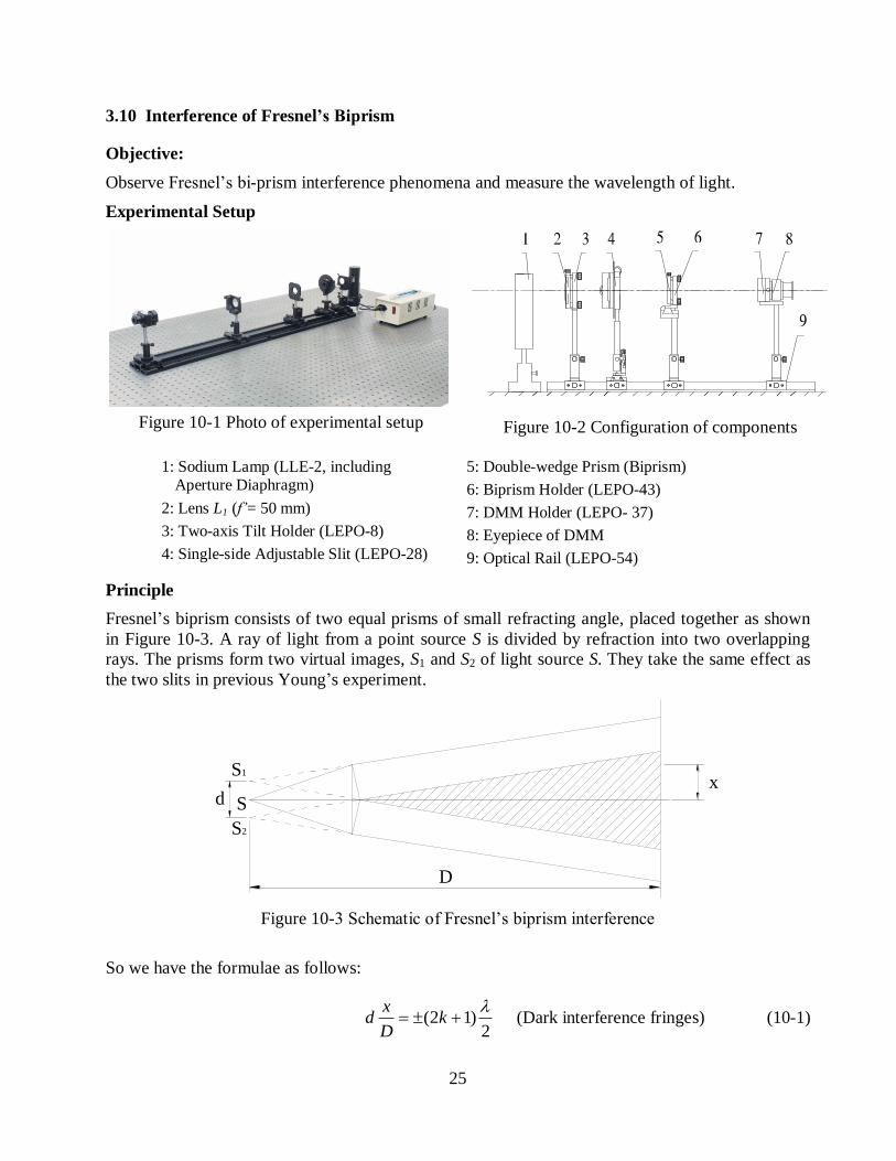
Experimental Setup
Figure 10-1 Photo of experimental setup
Figure 10-2 Configuration of components
1: Sodium Lamp (LLE-2, including
Aperture Diaphragm)
2: Lens L1 (f’= 50 mm)
3: Two-axis Tilt Holder (LEPO-8)
4: Single-side Adjustable Slit (LEPO-28)
5: Double-wedge Prism (Biprism)
6: Biprism Holder (LEPO-43)
7: DMM Holder (LEPO- 37)
8: Eyepiece of DMM
9: Optical Rail (LEPO-54)
Principle
Fresnel’s biprism consists of two equal prisms of small refracting angle, placed together as shown
in Figure 10-3. A ray of light from a point source S is divided by refraction into two overlapping
rays. The prisms form two virtual images, S1 and S2 of light source S. They take the same effect as
the two slits in previous Young’s experiment.
x
D
d S
S2
S1
Figure 10-3 Schematic of Fresnel’s biprism interference
So we have the formulae as follows:
2)12(
kD
xd (Dark interference fringes) (10-1)
26
kD
xd (Bright interference fringes) (10-2)
d
Dx (10-3)
where D is the distance between the point source and the viewing screen, x is the vertical distance
between the point source and viewing location on the screen, x is the distance between two
adjacent dark fringes (or bright fringes), d is the distance between the two virtual images S1 and S2.
d cannot be measured directly. But if we put a lens behind the biprism and measure the distance
between the images of S1 and S2 with the eyepiece of a DMM, then d can be calculated.
Experimental Procedures:
1) Refer to Figure 10-2, align all components in same height on the rail;
2) Focus the aperture of the light source onto the single slit by a lens. The key to the success
of this experiment is to align the directions of single slit and the double-edge of biprism
parallel;
3) Use a direct measurement microscope to observe biprism interference pattern, hence,
equal-interval bright/dark fringe pairs will be observed;
4) Measure the fringe interval x between two adjacent fringes using a direct measurement
microscope, and measure the distance D between the single slit plate and the microscope;
5) To obtain the interval d between the two virtual images generated by the Fresnel’s biprism,
put a lens L2 (f’=190 mm) behind the biprism to image the two virtual images into real
images. Move the direct measurement microscope to the real images plane and measure the
distance between the two real images as d’, by the use of object-image relationship of lens
imaging (lens equation) to obtain d;
6) Use d, x, D and equation (10-3), to calculate the wavelength of the illumination light.
27
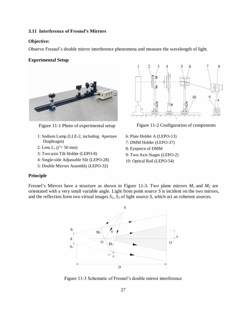
3.11 Interference of Fresnel’s Mirrors
Objective:
Observe Fresnel’s double mirror interference phenomena and measure the wavelength of light.
Experimental Setup
Figure 11-1 Photo of experimental setup
`
Figure 11-2 Configuration of components
1: Sodium Lamp (LLE-2, including Aperture
Diaphragm)
2: Lens L1 (f’= 50 mm)
3: Two-axis Tilt Holder (LEPO-8)
4: Single-side Adjustable Slit (LEPO-28)
5: Double Mirrors Assembly (LEPO-32)
6: Plate Holder A (LEPO-13)
7: DMM Holder (LEPO-37)
8: Eyepiece of DMM
9: Two-Axis Stages (LEPO-2)
10: Optical Rail (LEPO-54)
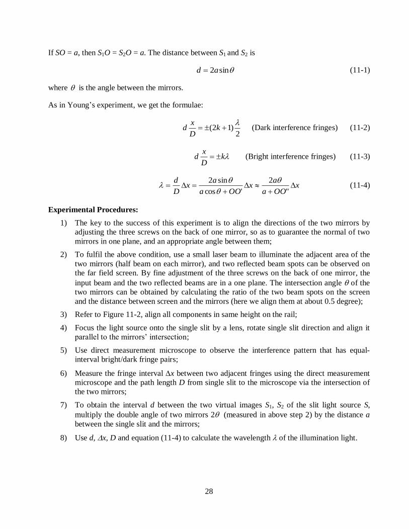
Principle
Fresnel’s Mirrors have a structure as shown in Figure 11-3. Two plane mirrors M1 and M2 are
orientated with a very small variable angle. Light from point source S is incident on the two mirrors,
and the reflection form two virtual images S1, S2 of light source S, which act as coherent sources.
O '
S1
S2
D
θ
S
M1
M2
dx
a
O
Figure 11-3 Schematic of Fresnel’s double mirror interference
28
If SO = a, then S1O = S2O = a. The distance between S1 and S2 is
sin2ad (11-1)
where is the angle between the mirrors.
As in Young’s experiment, we get the formulae:
2)12(
kD
xd (Dark interference fringes) (11-2)
kD
xd (Bright interference fringes) (11-3)
xOOa
ax
OOa
ax
D
d
"
2
'cos
sin2
(11-4)
Experimental Procedures:
1) The key to the success of this experiment is to align the directions of the two mirrors by
adjusting the three screws on the back of one mirror, so as to guarantee the normal of two
mirrors in one plane, and an appropriate angle between them;
2) To fulfil the above condition, use a small laser beam to illuminate the adjacent area of the
two mirrors (half beam on each mirror), and two reflected beam spots can be observed on
the far field screen. By fine adjustment of the three screws on the back of one mirror, the
input beam and the two reflected beams are in a one plane. The intersection angle of the
two mirrors can be obtained by calculating the ratio of the two beam spots on the screen
and the distance between screen and the mirrors (here we align them at about 0.5 degree);
3) Refer to Figure 11-2, align all components in same height on the rail;
4) Focus the light source onto the single slit by a lens, rotate single slit direction and align it
parallel to the mirrors’ intersection;
5) Use direct measurement microscope to observe the interference pattern that has equal-
interval bright/dark fringe pairs;
6) Measure the fringe interval x between two adjacent fringes using the direct measurement
microscope and the path length D from single slit to the microscope via the intersection of
the two mirrors;
7) To obtain the interval d between the two virtual images S1, S2 of the slit light source S,
multiply the double angle of two mirrors 2 (measured in above step 2) by the distance a
between the single slit and the mirrors;
8) Use d, x, D and equation (11-4) to calculate the wavelength of the illumination light.
29
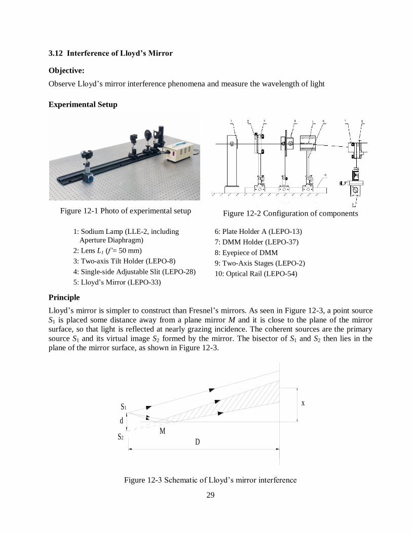
3.12 Interference of Lloyd’s Mirror
Objective:
Observe Lloyd’s mirror interference phenomena and measure the wavelength of light
Experimental Setup
Figure 12-1 Photo of experimental setup
Figure 12-2 Configuration of components
1: Sodium Lamp (LLE-2, including
Aperture Diaphragm)
2: Lens L1 (f’= 50 mm)
3: Two-axis Tilt Holder (LEPO-8)
4: Single-side Adjustable Slit (LEPO-28)
5: Lloyd’s Mirror (LEPO-33)
6: Plate Holder A (LEPO-13)
7: DMM Holder (LEPO-37)
8: Eyepiece of DMM
9: Two-Axis Stages (LEPO-2)
10: Optical Rail (LEPO-54)
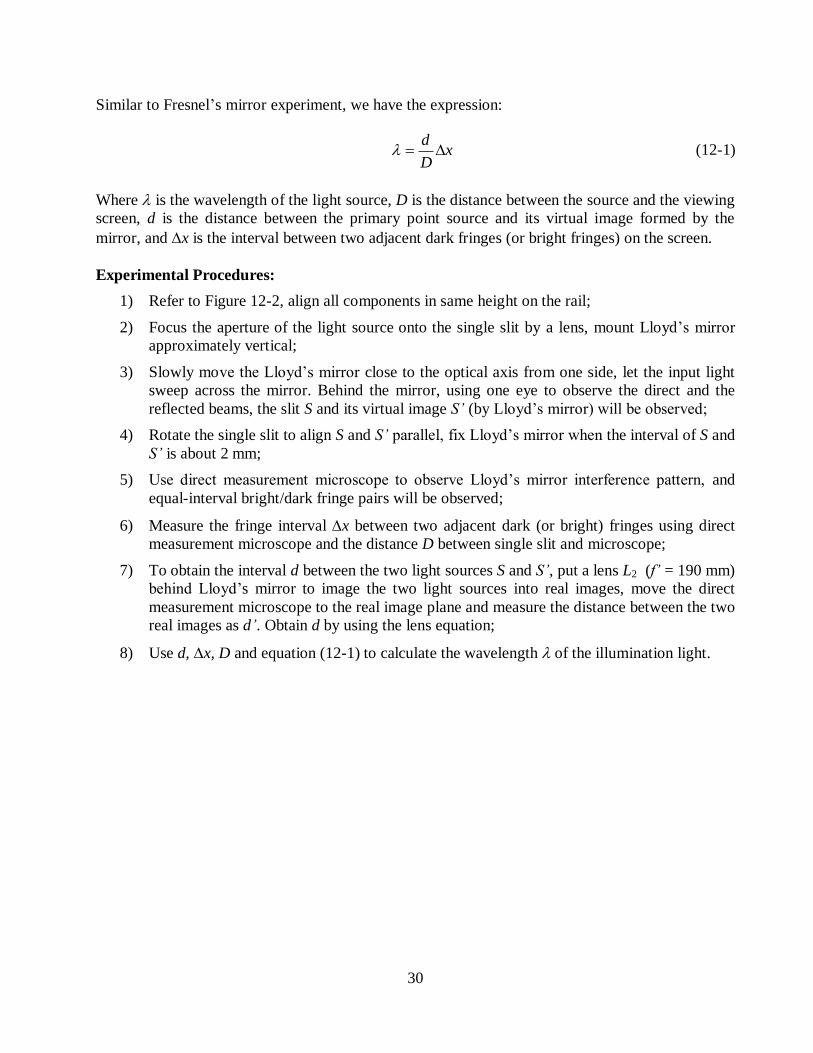
Principle
Lloyd’s mirror is simpler to construct than Fresnel’s mirrors. As seen in Figure 12-3, a point source
S1 is placed some distance away from a plane mirror M and it is close to the plane of the mirror
surface, so that light is reflected at nearly grazing incidence. The coherent sources are the primary
source S1 and its virtual image S2 formed by the mirror. The bisector of S1 and S2 then lies in the
plane of the mirror surface, as shown in Figure 12-3.
x
d
DS2
S1
M
Figure 12-3 Schematic of Lloyd’s mirror interference
30
Similar to Fresnel’s mirror experiment, we have the expression:
xD
d (12-1)
Where is the wavelength of the light source, D is the distance between the source and the viewing
screen, d is the distance between the primary point source and its virtual image formed by the
mirror, and x is the interval between two adjacent dark fringes (or bright fringes) on the screen.
Experimental Procedures:
1) Refer to Figure 12-2, align all components in same height on the rail;
2) Focus the aperture of the light source onto the single slit by a lens, mount Lloyd’s mirror
approximately vertical;
3) Slowly move the Lloyd’s mirror close to the optical axis from one side, let the input light
sweep across the mirror. Behind the mirror, using one eye to observe the direct and the
reflected beams, the slit S and its virtual image S’ (by Lloyd’s mirror) will be observed;
4) Rotate the single slit to align S and S’ parallel, fix Lloyd’s mirror when the interval of S and
S’ is about 2 mm;
5) Use direct measurement microscope to observe Lloyd’s mirror interference pattern, and
equal-interval bright/dark fringe pairs will be observed;
6) Measure the fringe interval x between two adjacent dark (or bright) fringes using direct
measurement microscope and the distance D between single slit and microscope;
7) To obtain the interval d between the two light sources S and S’, put a lens L2 (f’ = 190 mm)
behind Lloyd’s mirror to image the two light sources into real images, move the direct
measurement microscope to the real image plane and measure the distance between the two
real images as d’. Obtain d by using the lens equation;
8) Use d, x, D and equation (12-1) to calculate the wavelength of the illumination light.
31
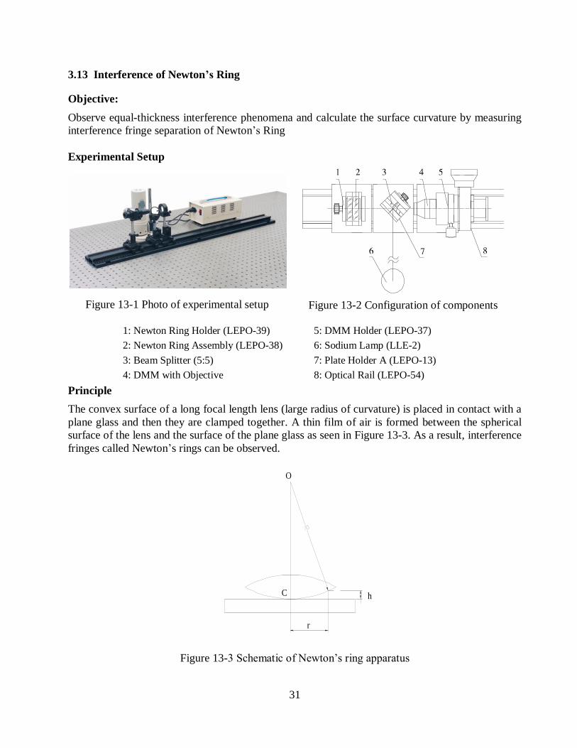
3.13 Interference of Newton’s Ring
Objective:
Observe equal-thickness interference phenomena and calculate the surface curvature by measuring
interference fringe separation of Newton’s Ring
Experimental Setup
Figure 13-1 Photo of experimental setup
Figure 13-2 Configuration of components
1: Newton Ring Holder (LEPO-39)
2: Newton Ring Assembly (LEPO-38)
3: Beam Splitter (5:5)
4: DMM with Objective
5: DMM Holder (LEPO-37)
6: Sodium Lamp (LLE-2)
7: Plate Holder A (LEPO-13)
8: Optical Rail (LEPO-54)
Principle
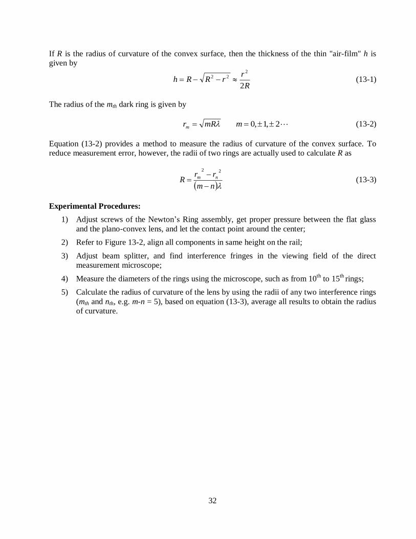
The convex surface of a long focal length lens (large radius of curvature) is placed in contact with a
plane glass and then they are clamped together. A thin film of air is formed between the spherical
surface of the lens and the surface of the plane glass as seen in Figure 13-3. As a result, interference
fringes called Newton’s rings can be observed.
O
h
r
C
Figure 13-3 Schematic of Newton’s ring apparatus
32
If R is the radius of curvature of the convex surface, then the thickness of the thin "air-film" h is
given by
R
rrRRh
2
222 (13-1)
The radius of the mth dark ring is given by
mRrm 2,1,0 m (13-2)
Equation (13-2) provides a method to measure the radius of curvature of the convex surface. To
reduce measurement error, however, the radii of two rings are actually used to calculate R as
nm
rrR nm
22
(13-3)
Experimental Procedures:
1) Adjust screws of the Newton’s Ring assembly, get proper pressure between the flat glass
and the plano-convex lens, and let the contact point around the center;
2) Refer to Figure 13-2, align all components in same height on the rail;
3) Adjust beam splitter, and find interference fringes in the viewing field of the direct
measurement microscope;
4) Measure the diameters of the rings using the microscope, such as from 10th
to 15th
rings;
5) Calculate the radius of curvature of the lens by using the radii of any two interference rings
(mth and nth, e.g. m-n = 5), based on equation (13-3), average all results to obtain the radius
of curvature.
33
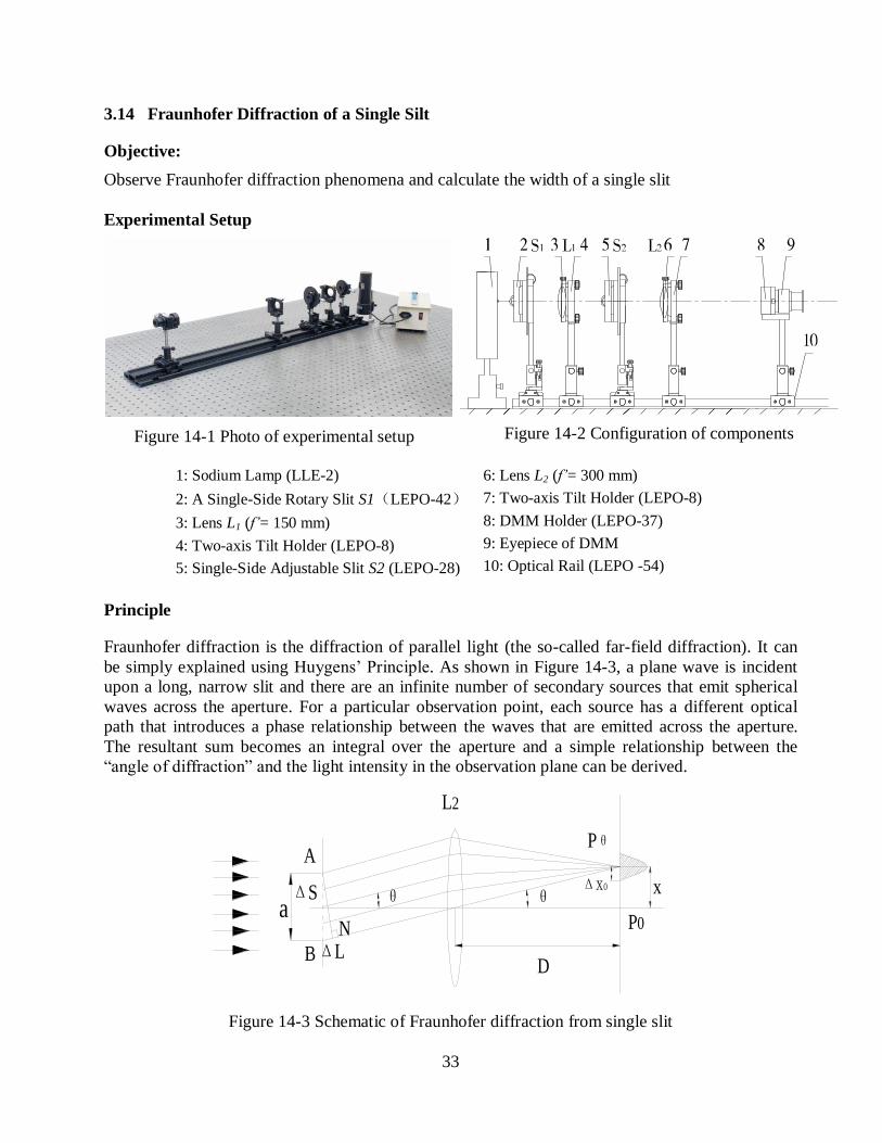
3.14 Fraunhofer Diffraction of a Single Silt
Objective:
Observe Fraunhofer diffraction phenomena and calculate the width of a single slit
Experimental Setup
Figure 14-1 Photo of experimental setup
Figure 14-2 Configuration of components
1: Sodium Lamp (LLE-2)
2: A Single-Side Rotary Slit S1(LEPO-42)
3: Lens L1 (f’= 150 mm)
4: Two-axis Tilt Holder (LEPO-8)
5: Single-Side Adjustable Slit S2 (LEPO-28)
6: Lens L2 (f’= 300 mm)
7: Two-axis Tilt Holder (LEPO-8)
8: DMM Holder (LEPO-37)
9: Eyepiece of DMM
10: Optical Rail (LEPO -54)
Principle
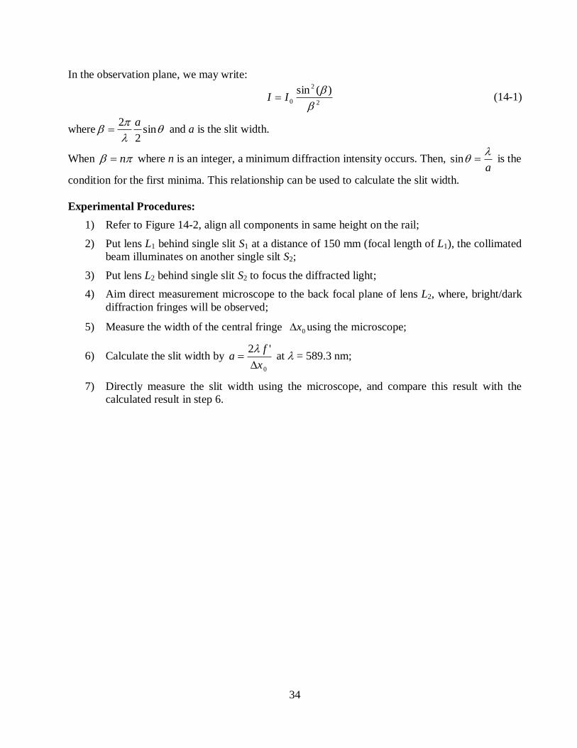
Fraunhofer diffraction is the diffraction of parallel light (the so-called far-field diffraction). It can
be simply explained using Huygens’ Principle. As shown in Figure 14-3, a plane wave is incident
upon a long, narrow slit and there are an infinite number of secondary sources that emit spherical
waves across the aperture. For a particular observation point, each source has a different optical
path that introduces a phase relationship between the waves that are emitted across the aperture.
The resultant sum becomes an integral over the aperture and a simple relationship between the
“angle of diffraction” and the light intensity in the observation plane can be derived.
D
Δx0 x
P0
Pθ
L2
ΔL
θ θΔS
N
B
A
a
Figure 14-3 Schematic of Fraunhofer diffraction from single slit
34
In the observation plane, we may write:
2
2
0
)(sin
II (14-1)
where
sin
2
2 a and a is the slit width.
When n where n is an integer, a minimum diffraction intensity occurs. Then, a
sin is the
condition for the first minima. This relationship can be used to calculate the slit width.
Experimental Procedures:
1) Refer to Figure 14-2, align all components in same height on the rail;
2) Put lens L1 behind single slit S1 at a distance of 150 mm (focal length of L1), the collimated
beam illuminates on another single silt S2;
3) Put lens L2 behind single slit S2 to focus the diffracted light;
4) Aim direct measurement microscope to the back focal plane of lens L2, where, bright/dark
diffraction fringes will be observed;
5) Measure the width of the central fringe 0x using the microscope;
6) Calculate the slit width by 0
'2
x
fa
at = 589.3 nm;
7) Directly measure the slit width using the microscope, and compare this result with the
calculated result in step 6.
35
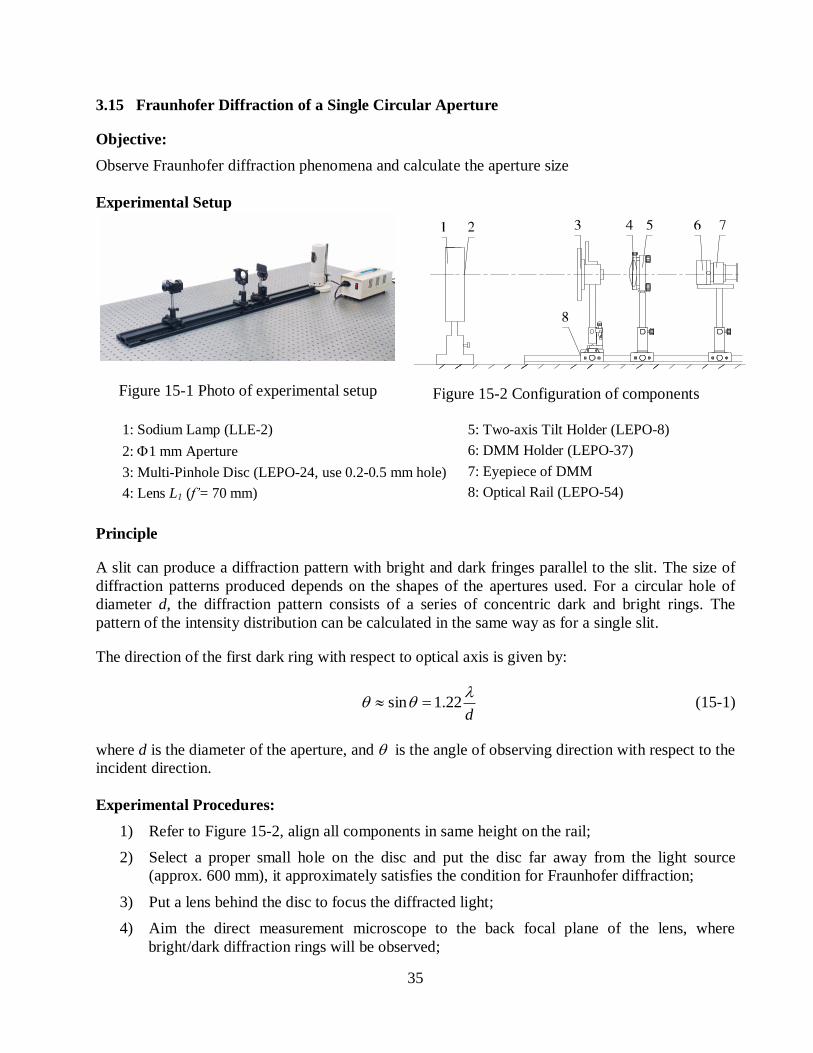
3.15 Fraunhofer Diffraction of a Single Circular Aperture
Objective:
Observe Fraunhofer diffraction phenomena and calculate the aperture size
Experimental Setup
Figure 15-1 Photo of experimental setup
Figure 15-2 Configuration of components
1: Sodium Lamp (LLE-2)
2: 1 mm Aperture
3: Multi-Pinhole Disc (LEPO-24, use 0.2-0.5 mm hole)
4: Lens L1 (f’= 70 mm)
5: Two-axis Tilt Holder (LEPO-8)
6: DMM Holder (LEPO-37)
7: Eyepiece of DMM
8: Optical Rail (LEPO-54)
Principle
A slit can produce a diffraction pattern with bright and dark fringes parallel to the slit. The size of
diffraction patterns produced depends on the shapes of the apertures used. For a circular hole of
diameter d, the diffraction pattern consists of a series of concentric dark and bright rings. The
pattern of the intensity distribution can be calculated in the same way as for a single slit.
The direction of the first dark ring with respect to optical axis is given by:
d
22.1sin (15-1)
where d is the diameter of the aperture, and is the angle of observing direction with respect to the
incident direction.
Experimental Procedures:
1) Refer to Figure 15-2, align all components in same height on the rail;
2) Select a proper small hole on the disc and put the disc far away from the light source
(approx. 600 mm), it approximately satisfies the condition for Fraunhofer diffraction;
3) Put a lens behind the disc to focus the diffracted light;
4) Aim the direct measurement microscope to the back focal plane of the lens, where
bright/dark diffraction rings will be observed;
36
5) Measure Airy disk diameter d1 using the microscope;
6) Calculate aperture diameter by 1
'22.1
d
fd
at = 589.3 nm;
7) Directly measure the aperture diameter using the microscope, compare this result with the
calculated result in step 6.
37
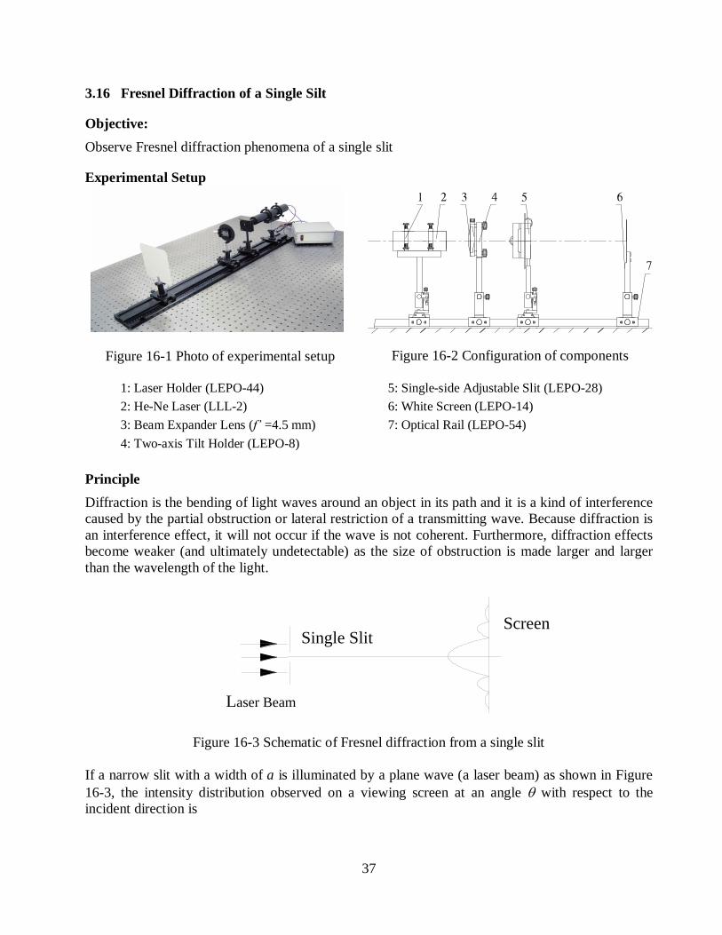
3.16 Fresnel Diffraction of a Single Silt
Objective:
Observe Fresnel diffraction phenomena of a single slit
Experimental Setup
Figure 16-1 Photo of experimental setup
Figure 16-2 Configuration of components
1: Laser Holder (LEPO-44)
2: He-Ne Laser (LLL-2)
3: Beam Expander Lens (f’ =4.5 mm)
4: Two-axis Tilt Holder (LEPO-8)
5: Single-side Adjustable Slit (LEPO-28)
6: White Screen (LEPO-14)
7: Optical Rail (LEPO-54)
Principle
Diffraction is the bending of light waves around an object in its path and it is a kind of interference
caused by the partial obstruction or lateral restriction of a transmitting wave. Because diffraction is
an interference effect, it will not occur if the wave is not coherent. Furthermore, diffraction effects
become weaker (and ultimately undetectable) as the size of obstruction is made larger and larger
than the wavelength of the light.
ScreenSingle Slit
Laser Beam
Figure 16-3 Schematic of Fresnel diffraction from a single slit
If a narrow slit with a width of a is illuminated by a plane wave (a laser beam) as shown in Figure
16-3, the intensity distribution observed on a viewing screen at an angle with respect to the
incident direction is
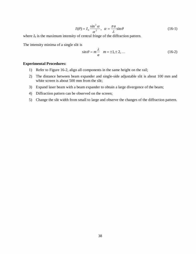
38
sin,
sin)(
2
2
0
aII (16-1)
where I0 is the maximum intensity of central fringe of the diffraction pattern.
The intensity minima of a single slit is
am
sin ,2,1 m … (16-2)
Experimental Procedures:
1) Refer to Figure 16-2, align all components in the same height on the rail;
2) The distance between beam expander and single-side adjustable slit is about 100 mm and
white screen is about 500 mm from the slit;
3) Expand laser beam with a beam expander to obtain a large divergence of the beam;
4) Diffraction pattern can be observed on the screen;
5) Change the slit width from small to large and observe the changes of the diffraction pattern.
39
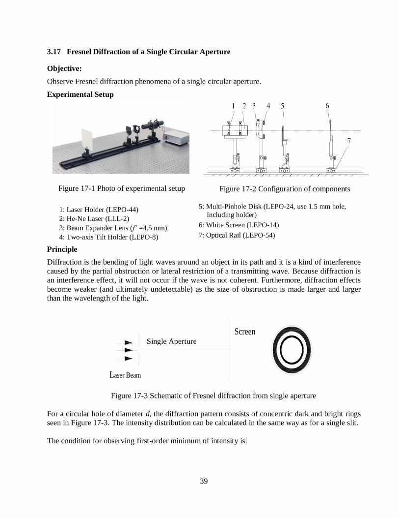
3.17 Fresnel Diffraction of a Single Circular Aperture
Objective:
Observe Fresnel diffraction phenomena of a single circular aperture.
Experimental Setup
Figure 17-1 Photo of experimental setup
Figure 17-2 Configuration of components
1: Laser Holder (LEPO-44)
2: He-Ne Laser (LLL-2)
3: Beam Expander Lens (f’ =4.5 mm)
4: Two-axis Tilt Holder (LEPO-8)
5: Multi-Pinhole Disk (LEPO-24, use 1.5 mm hole,
Including holder)
6: White Screen (LEPO-14)
7: Optical Rail (LEPO-54)
Principle
Diffraction is the bending of light waves around an object in its path and it is a kind of interference
caused by the partial obstruction or lateral restriction of a transmitting wave. Because diffraction is
an interference effect, it will not occur if the wave is not coherent. Furthermore, diffraction effects
become weaker (and ultimately undetectable) as the size of obstruction is made larger and larger
than the wavelength of the light.
Laser Beam
Single SlitScreen
Figure 17-3 Schematic of Fresnel diffraction from single aperture
For a circular hole of diameter d, the diffraction pattern consists of concentric dark and bright rings
seen in Figure 17-3. The intensity distribution can be calculated in the same way as for a single slit.
The condition for observing first-order minimum of intensity is:
Single Aperture
40
d
22.1sin (17-1)
where is the angle of observing direction with respect to the incident direction.
Experimental Procedures:
1) Refer to Figure 17-2, align all components in same height on the rail;
2) Expand laser beam using beam expander to obtain a large divergence of the beam;
3) Diffraction pattern can be observed on the screen;
4) Move the screen slowly away from the hole, the central portion of the diffraction pattern
will change from bright to dark alternatively.
41
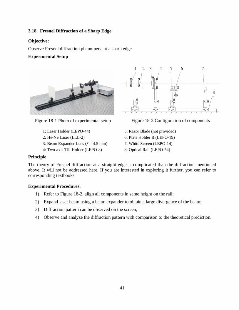
3.18 Fresnel Diffraction of a Sharp Edge
Objective:
Observe Fresnel diffraction phenomena at a sharp edge
Experimental Setup
Figure 18-1 Photo of experimental setup
Figure 18-2 Configuration of components
1: Laser Holder (LEPO-44)
2: He-Ne Laser (LLL-2)
3: Beam Expander Lens (f’ =4.5 mm)
4: Two-axis Tilt Holder (LEPO-8)
5: Razor Blade (not provided)
6: Plate Holder B (LEPO-19)
7: White Screen (LEPO-14)
8: Optical Rail (LEPO-54)
Principle
The theory of Fresnel diffraction at a straight edge is complicated than the diffraction mentioned
above. It will not be addressed here. If you are interested in exploring it further, you can refer to
corresponding textbooks.
Experimental Procedures:
1) Refer to Figure 18-2, align all components in same height on the rail;
2) Expand laser beam using a beam expander to obtain a large divergence of the beam;
3) Diffraction pattern can be observed on the screen;
4) Observe and analyze the diffraction pattern with comparison to the theoretical prediction.
42
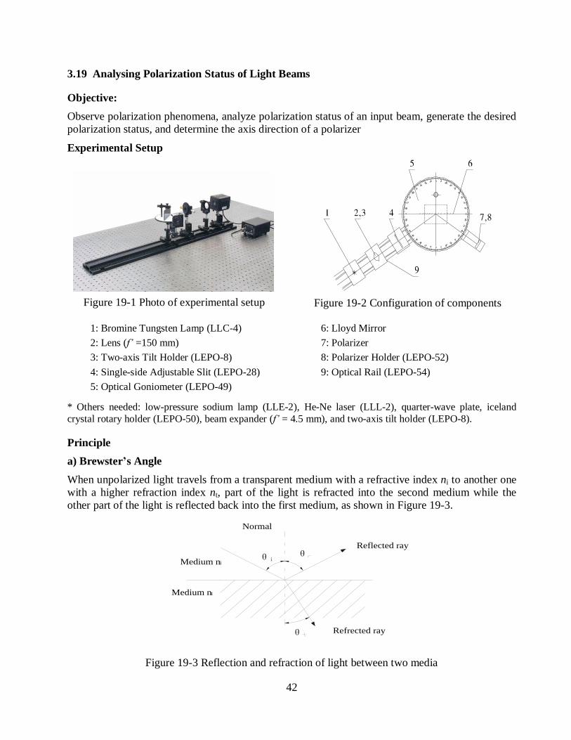
3.19 Analysing Polarization Status of Light Beams
Objective:
Observe polarization phenomena, analyze polarization status of an input beam, generate the desired
polarization status, and determine the axis direction of a polarizer
Experimental Setup
Figure 19-1 Photo of experimental setup
Figure 19-2 Configuration of components
1: Bromine Tungsten Lamp (LLC-4)
2: Lens (f’ =150 mm)
3: Two-axis Tilt Holder (LEPO-8)
4: Single-side Adjustable Slit (LEPO-28)
5: Optical Goniometer (LEPO-49)
6: Lloyd Mirror
7: Polarizer
8: Polarizer Holder (LEPO-52)
9: Optical Rail (LEPO-54)
* Others needed: low-pressure sodium lamp (LLE-2), He-Ne laser (LLL-2), quarter-wave plate, iceland
crystal rotary holder (LEPO-50), beam expander (f’ = 4.5 mm), and two-axis tilt holder (LEPO-8).
Principle
a) Brewster’s Angle
When unpolarized light travels from a transparent medium with a refractive index ni to another one
with a higher refraction index nt, part of the light is refracted into the second medium while the
other part of the light is reflected back into the first medium, as shown in Figure 19-3.
Refrected ray
Reflected rayθθi
θ
Normal
Medium nt
Medium ni
Figure 19-3 Reflection and refraction of light between two media
43
If the angles of incidence and refraction are i and t, respectively, the following condition exists,
known as Snell's law
nisin i =ntsin t (19-1)
According to Sir David Brewster, at a specific angle of incidence, b, called Brewster’s angle, the
reflected ray and the refracted ray are perpendicular to each other, so the sum of the incident angle
and the refractive angle is 90 as
90tb , namely bt 90 (19-2)
By substituting equation (19-2) into equation (19-1), we get
i
tb
btbtbi
n
n
nnn
tan
cos)90sin(sin
(19-3)
Then the Brewster’s angle is:
i
t
bn
narctan (19-4)
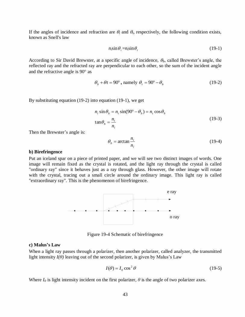
b) Birefringence
Put an iceland spar on a piece of printed paper, and we will see two distinct images of words. One
image will remain fixed as the crystal is rotated, and the light ray through the crystal is called
"ordinary ray" since it behaves just as a ray through glass. However, the other image will rotate
with the crystal, tracing out a small circle around the ordinary image. This light ray is called
"extraordinary ray". This is the phenomenon of birefringence.
e ray
o ray
Figure 19-4 Schematic of birefringence
c) Malus’s Law
When a light ray passes through a polarizer, then another polarizer, called analyzer, the transmitted
light intensity I(θ) leaving out of the second polarizer, is given by Malus’s Law
2
0 cos)( II (19-5)
Where I0 is light intensity incident on the first polarizer, θ is the angle of two polarizer axes.
44
Experimental Procedures:
1) Determine the polarization direction of a polarizer: the Tungsten lamp beam is incident on
the surface of a glass plate at an angle close to the Brewster’s angle of 57, rotate the
polarizer, directly observe the reflected beam, when it becomes the darkest, the polarizer
axis lays in the plane of incident and reflection beams;
2) Determine the axis of ½ wave plate: use a He-Ne laser as light source, insert a ½ wave
plate between two orthogonal polarizers with known axis directions, rotate the analyser to
find darkest direction by observing on a white viewing card/screen, the angle between the
axes of the ½ wave plate and the polarizer will be a half of the angle rotated by the
analyser;
3) Determine the axis of ¼ wave plate: use a He-Ne laser as light source, insert the ¼
wave plate between two orthogonal polarizers with known axis directions, when the angle
between polarizer and ¼ wave plate is 45 or 135, rotate the analyser and output light
intensity doesn’t change, therefore the axis of ¼ wave plate will be at 45 or 135 with
respect to the polarizer axis;
4) Rotate the analyser to verify Malus’s law;
5) Generate and analyze circular polarization beam and elliptical polarization beam.
45
3.20 Diffraction of a Grating
Objective:
Observe grating dispersion phenomena, and learn how to make wavelength measurement
Experimental Setup
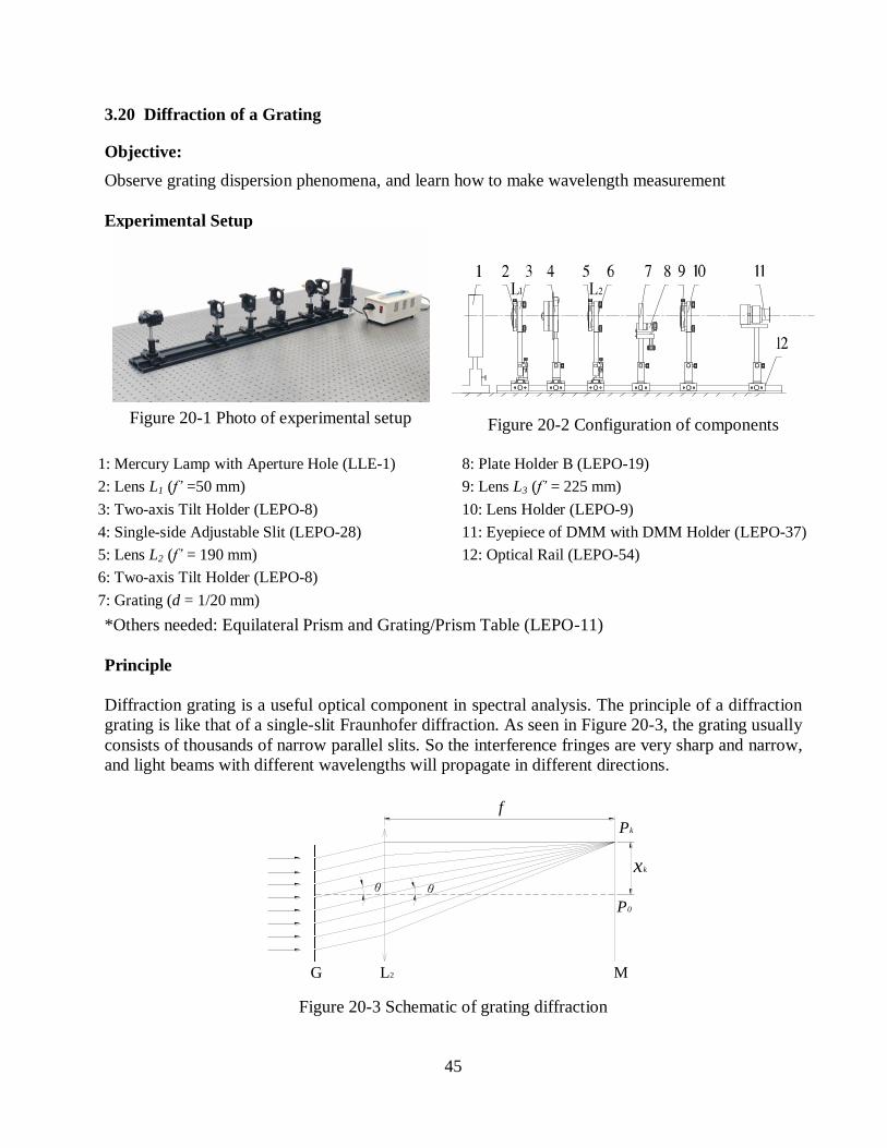
Figure 20-1 Photo of experimental setup
Figure 20-2 Configuration of components
1: Mercury Lamp with Aperture Hole (LLE-1)
2: Lens L1 (f’ =50 mm)
3: Two-axis Tilt Holder (LEPO-8)
4: Single-side Adjustable Slit (LEPO-28)
5: Lens L2 (f’ = 190 mm)
6: Two-axis Tilt Holder (LEPO-8)
7: Grating (d = 1/20 mm)
8: Plate Holder B (LEPO-19)
9: Lens L3 (f’ = 225 mm)
10: Lens Holder (LEPO-9)
11: Eyepiece of DMM with DMM Holder (LEPO-37)
12: Optical Rail (LEPO-54)
*Others needed: Equilateral Prism and Grating/Prism Table (LEPO-11)
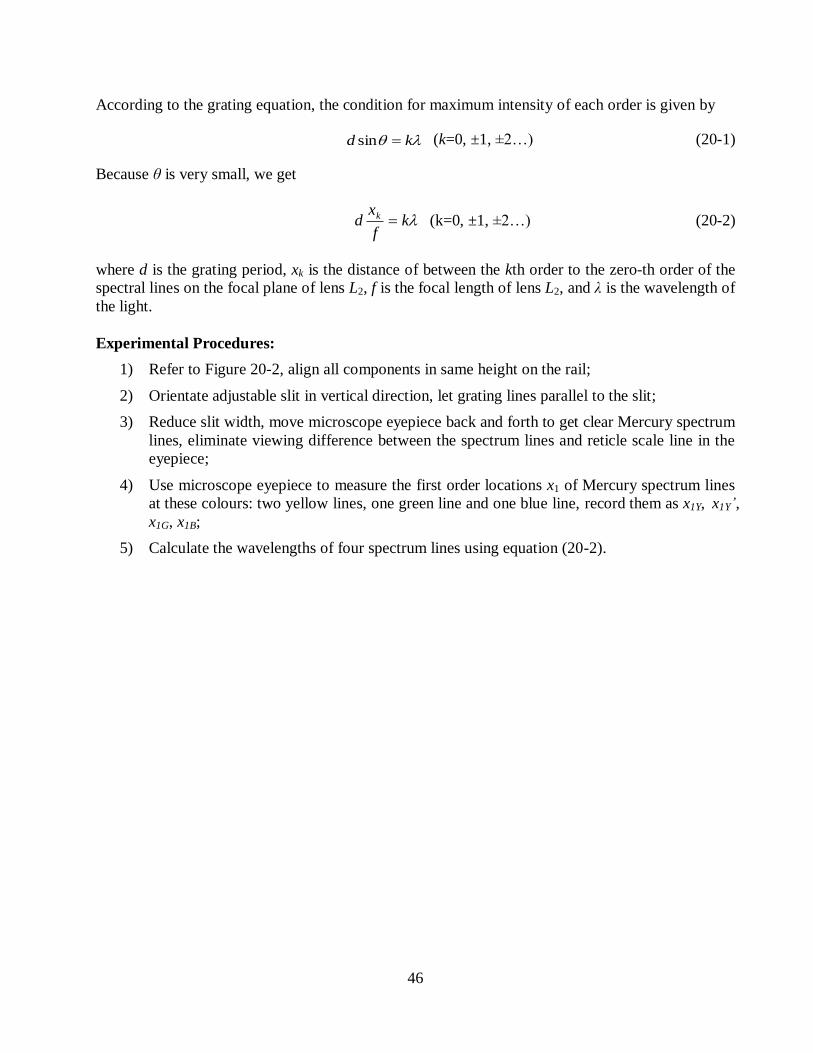
Principle
Diffraction grating is a useful optical component in spectral analysis. The principle of a diffraction
grating is like that of a single-slit Fraunhofer diffraction. As seen in Figure 20-3, the grating usually
consists of thousands of narrow parallel slits. So the interference fringes are very sharp and narrow,
and light beams with different wavelengths will propagate in different directions.
f
M
P0
θ
L2G
θ
Pk
xk
Figure 20-3 Schematic of grating diffraction
46
According to the grating equation, the condition for maximum intensity of each order is given by
kd sin (k=0, ±1, ±2…) (20-1)
Because θ is very small, we get
kf
xd k (k=0, ±1, ±2…) (20-2)
where d is the grating period, xk is the distance of between the kth order to the zero-th order of the
spectral lines on the focal plane of lens L2, f is the focal length of lens L2, and λ is the wavelength of
the light.
Experimental Procedures:
1) Refer to Figure 20-2, align all components in same height on the rail;
2) Orientate adjustable slit in vertical direction, let grating lines parallel to the slit;
3) Reduce slit width, move microscope eyepiece back and forth to get clear Mercury spectrum
lines, eliminate viewing difference between the spectrum lines and reticle scale line in the
eyepiece;
4) Use microscope eyepiece to measure the first order locations x1 of Mercury spectrum lines
at these colours: two yellow lines, one green line and one blue line, record them as x1Y, x1Y’,
x1G, x1B;
5) Calculate the wavelengths of four spectrum lines using equation (20-2).
47
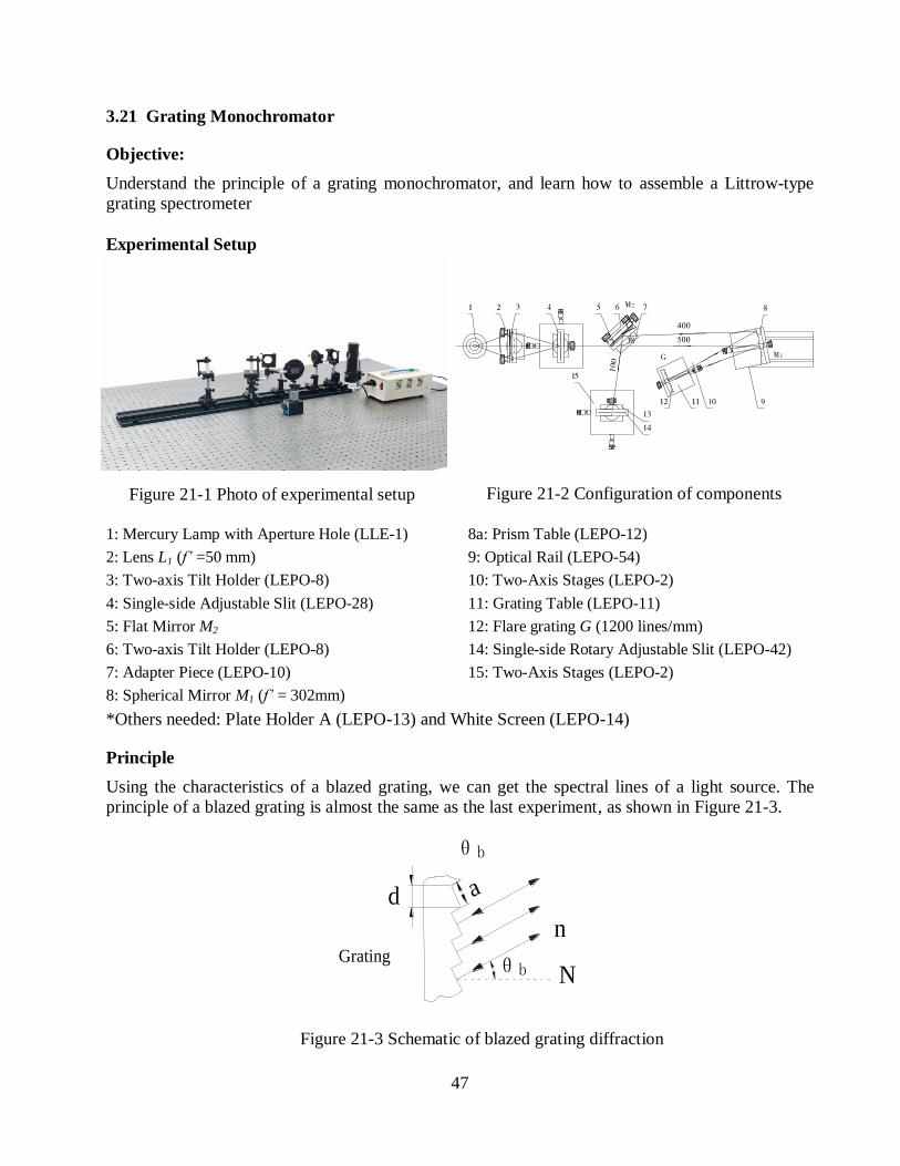
3.21 Grating Monochromator
Objective:
Understand the principle of a grating monochromator, and learn how to assemble a Littrow-type
grating spectrometer
Experimental Setup
Figure 21-1 Photo of experimental setup
Figure 21-2 Configuration of components
1: Mercury Lamp with Aperture Hole (LLE-1)
2: Lens L1 (f’ =50 mm)
3: Two-axis Tilt Holder (LEPO-8)
4: Single-side Adjustable Slit (LEPO-28)
5: Flat Mirror M2
6: Two-axis Tilt Holder (LEPO-8)
7: Adapter Piece (LEPO-10)
8: Spherical Mirror M1 (f’ = 302mm)
8a: Prism Table (LEPO-12)
9: Optical Rail (LEPO-54)
10: Two-Axis Stages (LEPO-2)
11: Grating Table (LEPO-11)
12: Flare grating G (1200 lines/mm)
14: Single-side Rotary Adjustable Slit (LEPO-42)
15: Two-Axis Stages (LEPO-2)
*Others needed: Plate Holder A (LEPO-13) and White Screen (LEPO-14)
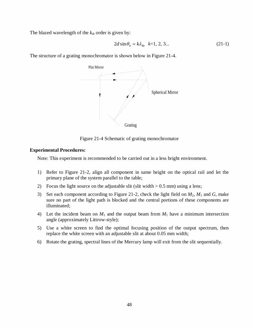
Principle
Using the characteristics of a blazed grating, we can get the spectral lines of a light source. The
principle of a blazed grating is almost the same as the last experiment, as shown in Figure 21-3.
Gratingθb N
n
ad
θb
Figure 21-3 Schematic of blazed grating diffraction
48
The blazed wavelength of the kth order is given by:
kbb kd sin2 k=1, 2, 3... (21-1)
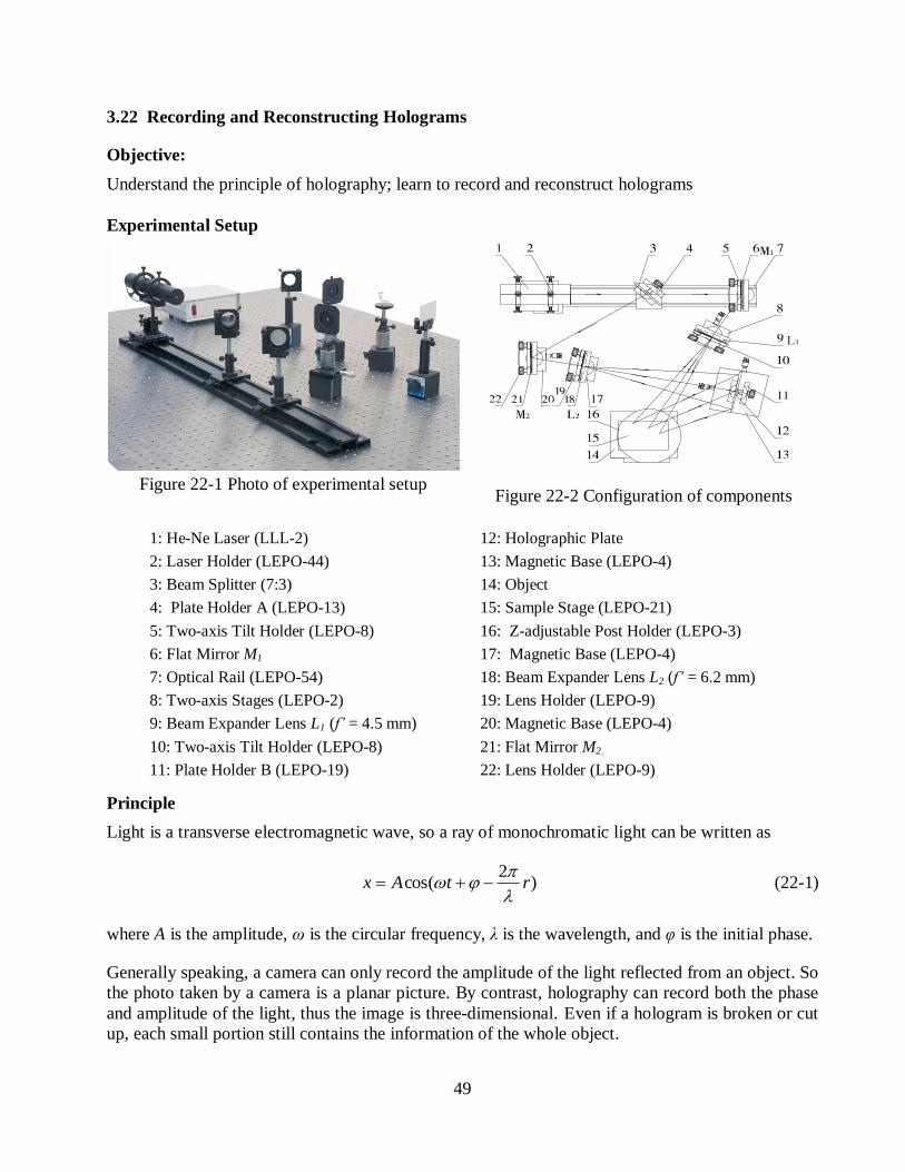
The structure of a grating monochromator is shown below in Figure 21-4.
Grating
Plat Mirror
Spherical Mirror
Figure 21-4 Schematic of grating monochromator
Experimental Procedures:
Note: This experiment is recommended to be carried out in a less bright environment.
1) Refer to Figure 21-2, align all component in same height on the optical rail and let the
primary plane of the system parallel to the table;
2) Focus the light source on the adjustable slit (slit width > 0.5 mm) using a lens;
3) Set each component according to Figure 21-2, check the light field on M2, M1 and G, make
sure no part of the light path is blocked and the central portions of these components are
illuminated;
4) Let the incident beam on M1 and the output beam from M1 have a minimum intersection
angle (approximately Littrow-style);
5) Use a white screen to find the optimal focusing position of the output spectrum, then
replace the white screen with an adjustable slit at about 0.05 mm width;
6) Rotate the grating, spectral lines of the Mercury lamp will exit from the slit sequentially.
49
3.22 Recording and Reconstructing Holograms
Objective:
Understand the principle of holography; learn to record and reconstruct holograms
Experimental Setup
Figure 22-1 Photo of experimental setup
Figure 22-2 Configuration of components
1: He-Ne Laser (LLL-2)
2: Laser Holder (LEPO-44)
3: Beam Splitter (7:3)
4: Plate Holder A (LEPO-13)
5: Two-axis Tilt Holder (LEPO-8)
6: Flat Mirror M1
7: Optical Rail (LEPO-54)
8: Two-axis Stages (LEPO-2)
9: Beam Expander Lens L1 (f’ = 4.5 mm)
10: Two-axis Tilt Holder (LEPO-8)
11: Plate Holder B (LEPO-19)
12: Holographic Plate
13: Magnetic Base (LEPO-4)
14: Object
15: Sample Stage (LEPO-21)
16: Z-adjustable Post Holder (LEPO-3)
17: Magnetic Base (LEPO-4)
18: Beam Expander Lens L2 (f’ = 6.2 mm)
19: Lens Holder (LEPO-9)
20: Magnetic Base (LEPO-4)
21: Flat Mirror M2
22: Lens Holder (LEPO-9)
Principle
Light is a transverse electromagnetic wave, so a ray of monochromatic light can be written as
)2
cos( rtAx
(22-1)
where A is the amplitude, ω is the circular frequency, λ is the wavelength, and φ is the initial phase.
Generally speaking, a camera can only record the amplitude of the light reflected from an object. So
the photo taken by a camera is a planar picture. By contrast, holography can record both the phase
and amplitude of the light, thus the image is three-dimensional. Even if a hologram is broken or cut
up, each small portion still contains the information of the whole object.
50
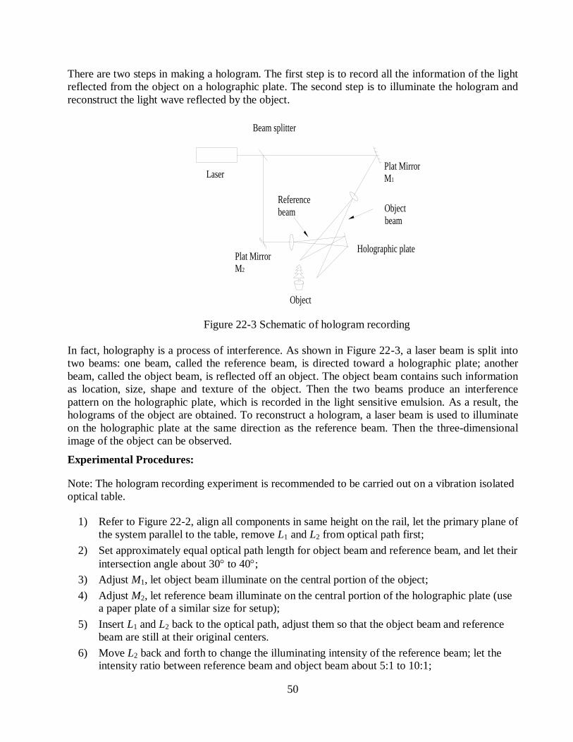
There are two steps in making a hologram. The first step is to record all the information of the light
reflected from the object on a holographic plate. The second step is to illuminate the hologram and
reconstruct the light wave reflected by the object.
Object
beam
Reference
beam
Object
Holographic platePlat Mirror M2
Beam splitter
Plat Mirror M1
Laser
Figure 22-3 Schematic of hologram recording
In fact, holography is a process of interference. As shown in Figure 22-3, a laser beam is split into
two beams: one beam, called the reference beam, is directed toward a holographic plate; another
beam, called the object beam, is reflected off an object. The object beam contains such information
as location, size, shape and texture of the object. Then the two beams produce an interference
pattern on the holographic plate, which is recorded in the light sensitive emulsion. As a result, the
holograms of the object are obtained. To reconstruct a hologram, a laser beam is used to illuminate
on the holographic plate at the same direction as the reference beam. Then the three-dimensional
image of the object can be observed.
Experimental Procedures:
Note: The hologram recording experiment is recommended to be carried out on a vibration isolated
optical table.
1) Refer to Figure 22-2, align all components in same height on the rail, let the primary plane of
the system parallel to the table, remove L1 and L2 from optical path first;
2) Set approximately equal optical path length for object beam and reference beam, and let their
intersection angle about 30 to 40;
3) Adjust M1, let object beam illuminate on the central portion of the object;
4) Adjust M2, let reference beam illuminate on the central portion of the holographic plate (use a paper plate of a similar size for setup);
5) Insert L1 and L2 back to the optical path, adjust them so that the object beam and reference
beam are still at their original centers.
6) Move L2 back and forth to change the illuminating intensity of the reference beam; let the intensity ratio between reference beam and object beam about 5:1 to 10:1;
51
7) Fix all components, turn off indoors light, replace the paper plate with a holographic plate and expose the holographic plate with He-Ne laser for 10 to 15 seconds;
8) Develop and fix the hologram;
9) Put back the hologram at its original location, remove object and block object beam, observe
the reconstructed object.
52
3.23 Making Holographic Gratings
Objective:
Understand the principle of holographic gratings, and learn how to fabricate holographic gratings
Experimental Setup
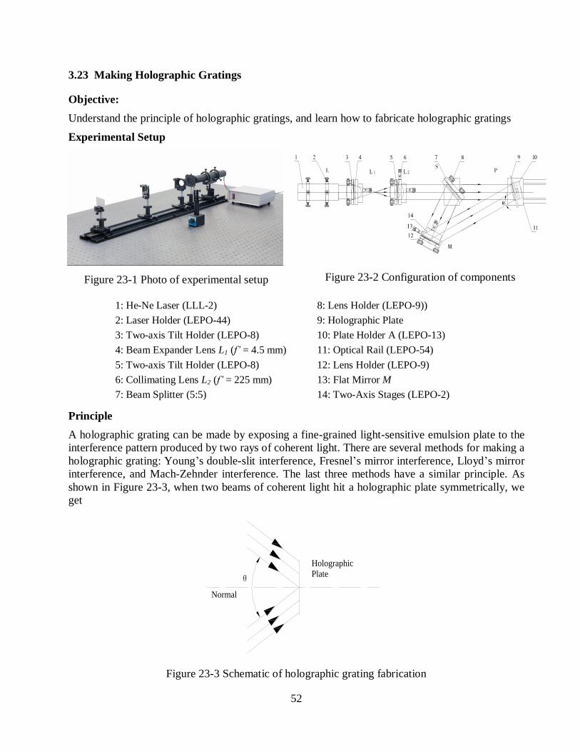
Figure 23-1 Photo of experimental setup
Figure 23-2 Configuration of components
1: He-Ne Laser (LLL-2)
2: Laser Holder (LEPO-44)
3: Two-axis Tilt Holder (LEPO-8)
4: Beam Expander Lens L1 (f’ = 4.5 mm)
5: Two-axis Tilt Holder (LEPO-8)
6: Collimating Lens L2 (f’ = 225 mm)
7: Beam Splitter (5:5)
8: Lens Holder (LEPO-9))
9: Holographic Plate
10: Plate Holder A (LEPO-13)
11: Optical Rail (LEPO-54)
12: Lens Holder (LEPO-9)
13: Flat Mirror M
14: Two-Axis Stages (LEPO-2)
Principle
A holographic grating can be made by exposing a fine-grained light-sensitive emulsion plate to the
interference pattern produced by two rays of coherent light. There are several methods for making a
holographic grating: Young’s double-slit interference, Fresnel’s mirror interference, Lloyd’s mirror
interference, and Mach-Zehnder interference. The last three methods have a similar principle. As
shown in Figure 23-3, when two beams of coherent light hit a holographic plate symmetrically, we
get
θ
Normal
Holographic
Plate
Figure 23-3 Schematic of holographic grating fabrication
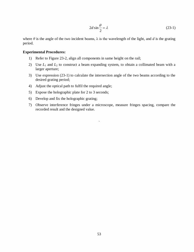
53
2sin2d (23-1)
where θ is the angle of the two incident beams, λ is the wavelength of the light, and d is the grating
period.
Experimental Procedures:
1) Refer to Figure 23-2, align all components in same height on the rail;
2) Use L1 and L2 to construct a beam expanding system, to obtain a collimated beam with a
larger aperture;
3) Use expression (23-1) to calculate the intersection angle of the two beams according to the
desired grating period;
4) Adjust the optical path to fulfil the required angle;
5) Expose the holographic plate for 2 to 3 seconds;
6) Develop and fix the holographic grating;
7) Observe interference fringes under a microscope, measure fringes spacing, compare the
recorded result and the designed value.
`
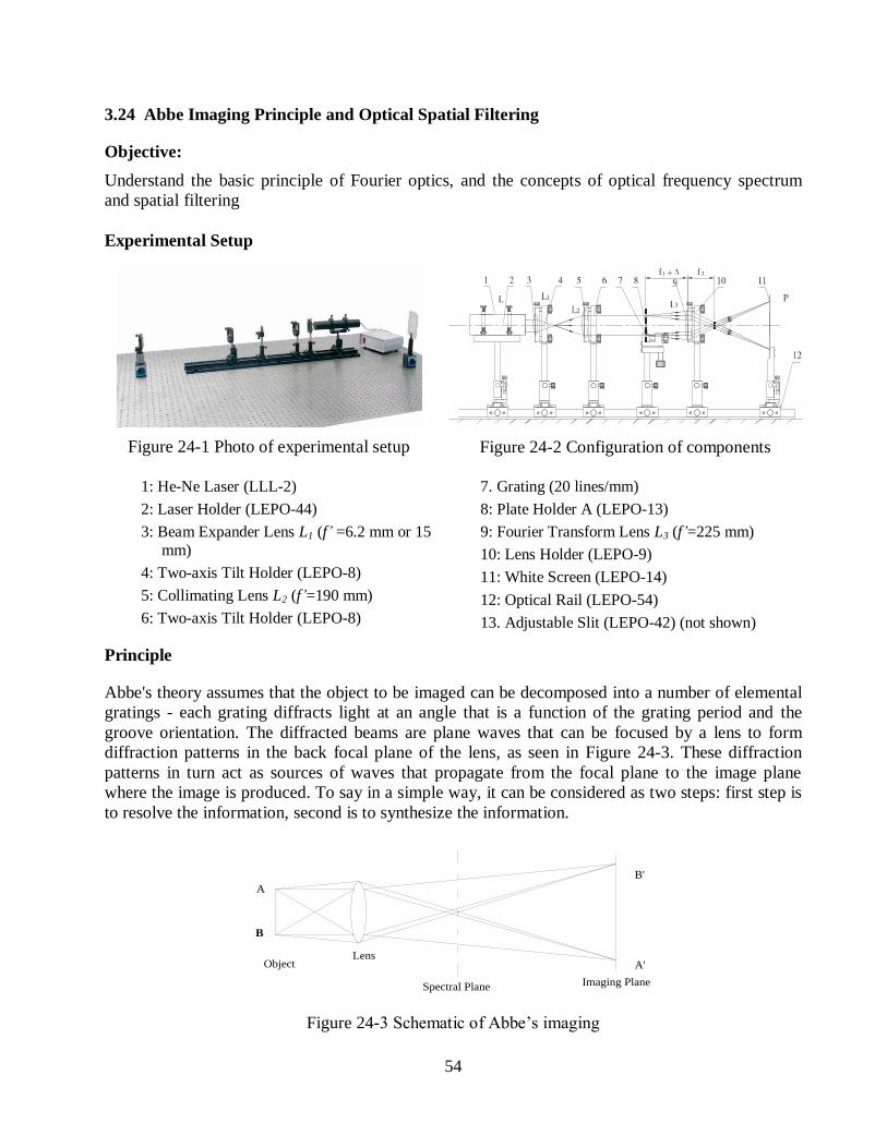
54
3.24 Abbe Imaging Principle and Optical Spatial Filtering
Objective:
Understand the basic principle of Fourier optics, and the concepts of optical frequency spectrum
and spatial filtering
Experimental Setup
Figure 24-1 Photo of experimental setup
Figure 24-2 Configuration of components
1: He-Ne Laser (LLL-2)
2: Laser Holder (LEPO-44)
3: Beam Expander Lens L1 (f’ =6.2 mm or 15
mm)
4: Two-axis Tilt Holder (LEPO-8)
5: Collimating Lens L2 (f’=190 mm)
6: Two-axis Tilt Holder (LEPO-8)
7. Grating (20 lines/mm)
8: Plate Holder A (LEPO-13)
9: Fourier Transform Lens L3 (f’=225 mm)
10: Lens Holder (LEPO-9)
11: White Screen (LEPO-14)
12: Optical Rail (LEPO-54)
13. Adjustable Slit (LEPO-42) (not shown)
Principle
Abbe's theory assumes that the object to be imaged can be decomposed into a number of elemental
gratings - each grating diffracts light at an angle that is a function of the grating period and the
groove orientation. The diffracted beams are plane waves that can be focused by a lens to form
diffraction patterns in the back focal plane of the lens, as seen in Figure 24-3. These diffraction
patterns in turn act as sources of waves that propagate from the focal plane to the image plane
where the image is produced. To say in a simple way, it can be considered as two steps: first step is
to resolve the information, second is to synthesize the information.
B'
A'
Imaging Plane
Lens
B
A
Object
Spectral Plane
Figure 24-3 Schematic of Abbe’s imaging
55
Experimental Procedures:
1) Refer to Figure 24-2, align all components in same height along the rail;
2) Use L1 and L2 to construct a beam expanding system, to obtain a collimated beam with a
larger aperture and illuminate on the transmission grating (1-D grating) whose grating
grooves are in vertical direction;
3) Put a screen P away from the grating about 2 meters, move the transform lens L3 back and
forth to form a clear grating image on the screen;
4) Insert an adjustable slit at the back focal plane of L3, block all higher-order spectra except
the zero-th order, check whether there are still grating lines in the image;
5) Adjust the slit width so that the zero-th order and the first order spectra pass through,
observe the grating image, then remove slit, observe grating image again, compare the two
cases;
6) Replace the transmission grating (1-D grating) with a 2-D grating, put a adjustable slit on
the Fourier plane and set slit direction in vertical direction to pass the spectrum on Y axis,
observe the direction of the grating lines on the image screen;
7) Rotate slit direction by 90 to let the X axis spectrum pass, observe the direction of the
grating lines on the image screen;
8) Further rotate slit direction by 45, observe the direction of grating lines direction on the
image screen;
9) Put an iris diaphragm on the Fourier plane, reduce its aperture slowly, till only the zero-th
order passes through, observe the image on screen;
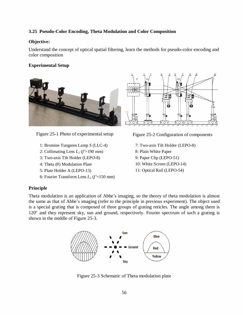
56
3.25 Pseudo-Color Encoding, Theta Modulation and Color Composition
Objective:
Understand the concept of optical spatial filtering, learn the methods for pseudo-color encoding and
color composition
Experimental Setup
Figure 25-1 Photo of experimental setup
Figure 25-2 Configuration of components
1: Bromine Tungsten Lamp S (LLC-4)
2: Collimating Lens L1 (f’=190 mm)
3: Two-axis Tilt Holder (LEPO-8)
4: Theta () Modulation Plate
5: Plate Holder A (LEPO-13)
6: Fourier Transform Lens L2 (f’=150 mm)
7: Two-axis Tilt Holder (LEPO-8)
8: Plain White Paper
9: Paper Clip (LEPO-51)
10: White Screen (LEPO-14)
11: Optical Rail (LEPO-54)
Principle
Theta modulation is an application of Abbe’s imaging, so the theory of theta modulation is almost
the same as that of Abbe’s imaging (refer to the principle in previous experiment). The object used
is a special grating that is composed of three groups of grating reticles. The angle among them is
120 and they represent sky, sun and ground, respectively. Fourier spectrum of such a grating is
shown in the middle of Figure 25-3.
Figure 25-3 Schematic of Theta modulation plate
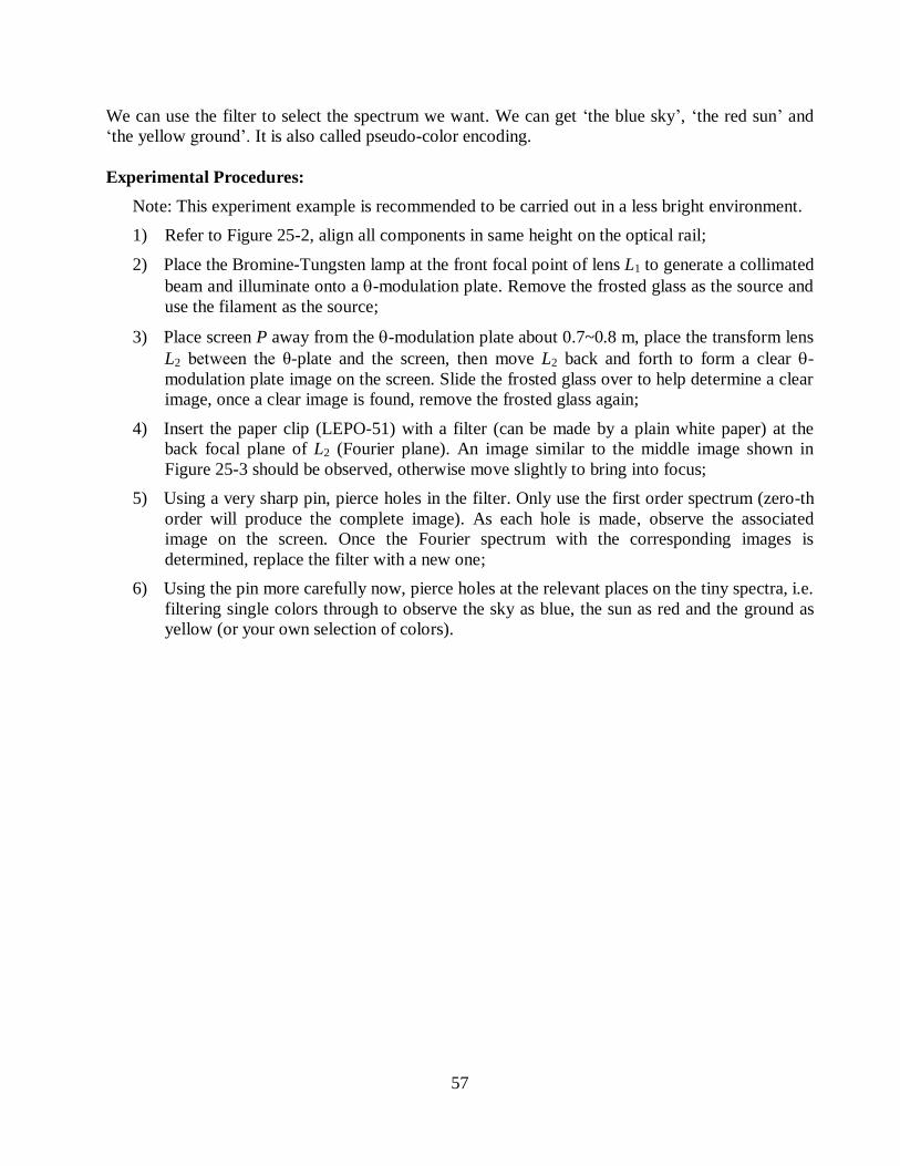
57
We can use the filter to select the spectrum we want. We can get ‘the blue sky’, ‘the red sun’ and
‘the yellow ground’. It is also called pseudo-color encoding.
Experimental Procedures:
Note: This experiment example is recommended to be carried out in a less bright environment.
1) Refer to Figure 25-2, align all components in same height on the optical rail;
2) Place the Bromine-Tungsten lamp at the front focal point of lens L1 to generate a collimated
beam and illuminate onto a -modulation plate. Remove the frosted glass as the source and
use the filament as the source;
3) Place screen P away from the -modulation plate about 0.7~0.8 m, place the transform lens
L2 between the θ-plate and the screen, then move L2 back and forth to form a clear -
modulation plate image on the screen. Slide the frosted glass over to help determine a clear
image, once a clear image is found, remove the frosted glass again;
4) Insert the paper clip (LEPO-51) with a filter (can be made by a plain white paper) at the
back focal plane of L2 (Fourier plane). An image similar to the middle image shown in
Figure 25-3 should be observed, otherwise move slightly to bring into focus;
5) Using a very sharp pin, pierce holes in the filter. Only use the first order spectrum (zero-th
order will produce the complete image). As each hole is made, observe the associated
image on the screen. Once the Fourier spectrum with the corresponding images is
determined, replace the filter with a new one;
6) Using the pin more carefully now, pierce holes at the relevant places on the tiny spectra, i.e.
filtering single colors through to observe the sky as blue, the sun as red and the ground as
yellow (or your own selection of colors).
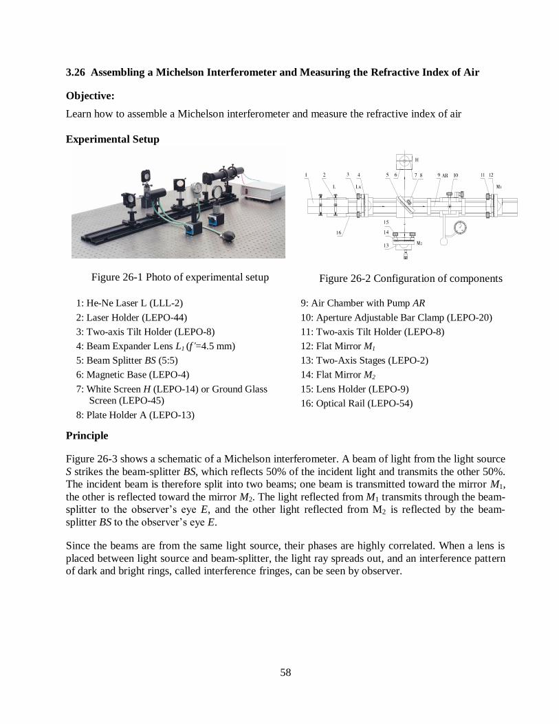
58
3.26 Assembling a Michelson Interferometer and Measuring the Refractive Index of Air
Objective:
Learn how to assemble a Michelson interferometer and measure the refractive index of air
Experimental Setup
Figure 26-1 Photo of experimental setup
Figure 26-2 Configuration of components
1: He-Ne Laser L (LLL-2)
2: Laser Holder (LEPO-44)
3: Two-axis Tilt Holder (LEPO-8)
4: Beam Expander Lens L1 (f’=4.5 mm)
5: Beam Splitter BS (5:5)
6: Magnetic Base (LEPO-4)
7: White Screen H (LEPO-14) or Ground Glass Screen (LEPO-45)
8: Plate Holder A (LEPO-13)
9: Air Chamber with Pump AR
10: Aperture Adjustable Bar Clamp (LEPO-20)
11: Two-axis Tilt Holder (LEPO-8)
12: Flat Mirror M1
13: Two-Axis Stages (LEPO-2)
14: Flat Mirror M2
15: Lens Holder (LEPO-9)
16: Optical Rail (LEPO-54)
Principle
Figure 26-3 shows a schematic of a Michelson interferometer. A beam of light from the light source
S strikes the beam-splitter BS, which reflects 50% of the incident light and transmits the other 50%.
The incident beam is therefore split into two beams; one beam is transmitted toward the mirror M1,
the other is reflected toward the mirror M2. The light reflected from M1 transmits through the beam-
splitter to the observer’s eye E, and the other light reflected from M2 is reflected by the beam-
splitter BS to the observer’s eye E.
Since the beams are from the same light source, their phases are highly correlated. When a lens is
placed between light source and beam-splitter, the light ray spreads out, and an interference pattern
of dark and bright rings, called interference fringes, can be seen by observer.
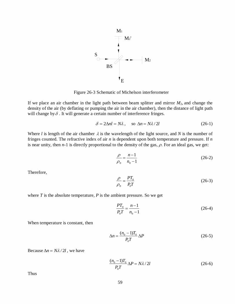
59
E
S
BS
M2'
M2
M1
Figure 26-3 Schematic of Michelson interferometer
If we place an air chamber in the light path between beam splitter and mirror M2, and change the
density of the air (by deflating or pumping the air in the air chamber), then the distance of light path
will change by . It will generate a certain number of interference fringes.
Nnl 2 , so lNn 2/ (26-1)
Where l is length of the air chamber is the wavelength of the light source, and N is the number of
fringes counted. The refractive index of air n is dependent upon both temperature and pressure. If n
is near unity, then n-1 is directly proportional to the density of the gas, . For an ideal gas, we get:
1
1
00
n
n
(26-2)
Therefore,
TP
PT
0
0
0
(26-3)
where T is the absolute temperature, P is the ambient pressure. So we get
1
1
00
0
n
n
TP
PT (26-4)
When temperature is constant, then
PTP
Tnn
0
00 )1( (26-5)
Because lNn 2/ , we have
lNPTP
Tn2/
)1(
0
00
(26-6)
Thus
60
P
P
l
Nn
21
(26-7)
Note: the standard atmospheric pressure is 101.3 kPa or 760 mm Hg.
Experimental Procedures:
1) Refer to Figure 26-2, align all components in same height on the rail;
2) Adjust the output of the He-Ne laser parallel along the optical rail (beam expander lens should not be inserted at this moment);
3) Put in a beam splitter BS at an angle of 45 with respect to beam axis, and adjust its tilt to make the two beams (transmission and reflection) parallel to table;
4) Adjust the tilt of mirrors M1 and M2 to make the reflected beams coincide with their incident
paths, and the two beam spots on the screen H overlap together;
5) Insert a beam expander L1, finely adjust beam splitter, M1 and M2, till concentric interference rings can be observed on the screen H;
6) Insert an air chamber between beam splitter and M1, adjust it parallel to optical path, pump
air into the air chamber till a maximum permit pressure (e.g. 40 kPa or 300 mm Hg) is
reached and write as P;
7) Slowly release the air valve, count the number of interference rings changed in the center till
air pressure falls to zero;
8) Repeat steps 6 and 7 several times to obtain averaged data;
9) Calculate the refractive index of air using equation (26-7).
61
4. Laser safety and lab requirements:
Follow the corresponding laser safety guidelines based on AS/NZS 2211.1:1997 and other lab
instructions about optical components etc.
Appendix: User Instructions of Silver Salt Plates
Silver salt plate is a common holographic recording medium with high sensitivity, broad spectral
response range, and wide adaptability. The micro particles of a silver salt plate make it suitable for
recording a variety of holograms. The drawbacks of silver salt plates are low diffraction efficiency
and low signal-to-noise ratio, together with tedious post-exposure processing procedures.
1. Specifications:
Wavelength: 632.8 nm
Contrast Ratio: >4
Sensitivity: >30 J/cm2
Thickness: ~ 7 m
Resolution: >3000 line pairs/mm
Cross Sectional Size: 90×240 mm
Storage: > 1 yr under low temperature environment of 0C to 7C such as in a refrigerator
Safety Lamp: Dark green lamp in a darkroom
2. Handling and Processing Procedures
1.1 Cutting of an unexposed silver salt plate
Before cutting a silver salt plate, place the container under room temperature for about 4 hours
and then open the container in a darkroom under the aid of a dark green safety lamp. Put the
film side of a silver salt plate down onto two plastic sticks and then cut the glass substrate side
from the top with a glass cutting knife into desired sizes. Knock the silver salt plate near the
cutting trace on the substrate side gently with the handle of the glass cutting knife and then
break the plate into two pieces with fingers. Wrap unused silver salt plates up with the black
paper and put back to the container.
1.2 Exposure of a silver salt plate
The typical size of micro particles with a silver salt plate is in the range of 0.03 to 0.09 m. The
smaller size of micro particles the lower photo sensitivity and higher resolution. For this reason,
the exposure time of silver salt plate is longer than that in conventional photography. In
addition, the exposure time of a silver salt plate depends on factors such as the laser power and
the reflectivity of an object. In practice, one had better use a small stripe of silver salt plate and
expose different locations of the stripe with different exposure time durations to determine an
optimal exposure time after post-exposure processes.
When putting a silver salt plate on a plate holder, make sure that the film side of the plate faces
towards the object under recording. Typically, the film side of a silver salt plate is stickier than
Note: Wear gloves during this process to avoid finger print on silver salt plates.
62
the glass substrate side when touched with moist fingers. Alternatively, the film side of a silver
salt plate can be determined under a dark green lamp in a darkroom. The side with higher light
reflection is the film side.
1.3 Preparation of developing and fixing solutions
The user can acquire developing and fixing solutions through the following two approaches:
Approach 1: acquire Kodak D-19 Developer Powder and Kodak Fixer (for black and white film
and paper) Powder from photographic supplies stores, makes solutions following their
instructions.
Approach 2: use formulas to make solutions. The following apparatus and chemicals are
needed:
A balance with a precision of 0.01 g; two 1-liter beakers; several glass bottles; a thermometer
with a reading scale up to 100 C; an electric furnace, and distilled water.
The most common chemical used for developing silver salt plates is D-19 from Kodak and the
fixing chemical is F-5. Use analytical reagent during the post-exposure process.
Formula of D-19 developing solution
Description Dose Function
Distilled Water 500 ml at 50C
Metol 2 g Developer for forming soft image
Anhydrous Sodium Sulfite 90 g Antioxidant protector
Hydroquinone 8 g Developer for forming hard image
Anhydrous Sodium Carbonate 48 g Accelerator
Potassium Bromide 5 g Suppressant inhibitor
Add more distilled water to reach 1000 ml
Formula of F-5 fixing solution
Description Dose Function
Distilled Water 800 ml at 50C
Sodium Thiosulfate 240 g Fixer to dissolve unexposed Silver Bromide
Anhydrous Sodium Sulfite 15 g Protector of Sodium Thiosulfate in acid
Acetic Acid 13.5 g Developing stopper by neutralizing developer
Boric Acid 7.5 g Hardening agent to harden film subtitles
Potassium Alum 15 g Suppressant inhibitor
Add more distilled water to reach 1000 ml
All the chemicals listed in the formulae should be weighed using the balance and poured in
sequence into the beaker containing distilled water at a temperature of approximately 50 C.
After pouring one chemical into the solution, wait until the chemical is fully dissolved in the
63
solution before pouring the next chemical into the solution. After all the chemicals are poured
and dissolved, add more distilled water to reach 1000 ml.
Development:
Under the aid of a green safety lamp, immerse the silver slat plate into the D-19 developing
solution with the film side facing down, and keep stirring the solution for about 2 minutes. Take
the silver salt plate from the developing solution and wash it with water for 30 seconds. During
this process, the temperature of the developing solution should be maintained at 20C.
Stopping Development:
The objective of development stopping is to stop the development of the photosensitive layer of
a silver salt plate. Hence, excessive developing liquid can be avoided so that the fixing solution
will not be diluted. Soak the developed silver salt plate in the inhibitor solution for 30 seconds
and then wash it with water for another 30 seconds.
Fixing:
Soak the silver salt plate in the fixing solution for 3 to 5 minutes and keep stirring the fixing
solution. During this process, the photosensitive layer of the silver salt plate will gradually
become transparent. Keep the fixing process even after the plate becomes totally transparent.
The total fixing time duration is approximately twice of that from the initial immersion to the
moment when the plate becomes totally transparent.
Washing:
Wash the fixed silver salt plate with running water for about 5 minutes. If multiple plates are
washed, make sure each plate is fully washed. Also make sure the temperature of the running
water does not exceed 25 C as otherwise the film may come off and be washed away.
Removal of Sensitizer:
Soak the silver salt plate in methanol or ethanol solution for 3 minutes
Drying:
Let the silver salt plate dry naturally. If the step of sensitizer removal is skipped, then the silver
salt plate should be washed with distilled water rather than tap water. Otherwise, the silver salt
plate may be contaminated by impurities from tap water.
1.4 Bleaching of silver salt holographic plate
Note: 1. Some chemicals used in the developing and fixing processes may be toxic. Some
gases given off during the processes are also toxic. Make sure that the processing darkroom is
equipped with good ventilation.
2. Some chemicals used in the developing and fixing processes are also corrosive. Make
sure to wear rubber gloves to protect hands from contacting these corrosive chemicals.
64
The hologram of a silver salt plate obtained after exposing, developing, and fixing processes is
an amplitude hologram. Affected by factors such as the size of photosensitive particles, the
intensity ratio between object and reference light, and post-exposure processing procedures, the
interference contrast of an amplitude hologram is low yielding diffraction efficiency of about
7%. The diffraction efficiency can be enhanced by bleaching the hologram to reduce metal
silver to transparent silver salt. This results in the variation of refractive index in the exposed
area of the silver salt plate so that an amplitude hologram is converted into a phase hologram.
The diffraction efficiency of a phase hologram can reach 30% ~ 40%.
Bleaching Formula 1
Reagent Ammonium Bichromate concentrated Sulfuric Acid Potassium Bromide Water
Dose 20 g 14 ml 92 g 1000 ml
Bleaching Formula 2
Reagent Mercuric Chloride Potassium Bromide Water
Dose 18 g 8 g 800 ml
After the fixing process, ambient light can be turned on to start the bleaching process. Soak the
silver salt plate in the bleaching solution and keep swinging the plate in the solution while
monitoring the color change of the plate. Take the plate out of the bleaching solution when the
black color of the plate dissolves away in the solution. Wash the plate with water and let it dry
naturally.


![arXiv:1001.1408v1 [math.NA] 9 Jan 2010 · 2018. 11. 6. · arXiv:1001.1408v1 [math.NA] 9 Jan 2010 DISCRETE HAMILTONIAN VARIATIONAL INTEGRATORS MELVIN LEOK AND JINGJING ZHANG Abstract](https://img.pdfslide.net/doc/110x75/60cba5086c5d4e69724e2cb9/arxiv10011408v1-mathna-9-jan-2010-2018-11-6-arxiv10011408v1-mathna.jpg)

![arXiv:0707.1196v1 [math.DS] 9 Jul 2007 · arXiv:0707.1196v1 [math.DS] 9 Jul 2007 NONLINEAR DYNAMICS OF THE 3D PENDULUM∗ NALIN A. CHATURVEDI†, TAEYOUNG LEE‡, MELVIN LEOK§, AND](https://img.pdfslide.net/doc/110x75/5c9c107c09d3f23b2a8b4732/arxiv07071196v1-mathds-9-jul-2007-arxiv07071196v1-mathds-9-jul-2007.jpg)