Lesson 1: Introduction to ArcGIS - Geology Departmentgeology.wlu.edu/harbor/geol260/tutor/bolstad/Lesson1_Arc10.pdf · GIS Fundamentals: Supplementary Lessons with ArcGIS Introduction

GIS Fundamentals: Supplementary Lessons with ArcGIS Introduction to ArcGIS

1

Lesson 1: Introduction to ArcGIS

What You’ll Learn: -Start ArcMap -Create a new map -Add data layers -Pan and zoom -Change data symbology -Change display properties -Set relative paths -Add layers to features

-Select data -Measure distances -Use raster -Create map layouts to print -Add legends, titles, North arrows, and other elements -Print a map to a PDF

Data for this exercise are located in the L1 subdirectory or the class web page. Videos for this exercise are located in the class web page. What You’ll Produce: Four maps, one of lakes and roads, one of wetlands, a third map of the Cloquet Forestry Center, and a fourth a map of topological errors. Background: This is the first in a series of introductory exercises for ArcGIS/ArcMap. These are practical skills that complement the theory and practice of GIS described in the textbook “GIS Fundamentals: A First Text on Geographic Information Systems”, by Paul Bolstad. We assume you have a functioning copy of ArcMap running on your computer. The exercises were developed with ArcGIS, ArcView version 10, student edition. There are a set of videos that supplement these lessons. They will be referenced during the lessons, in bold. The first video, Start ArcMap, describes these first few steps. Each lab assumes you have a copy of the lesson data files on a local drive.


2

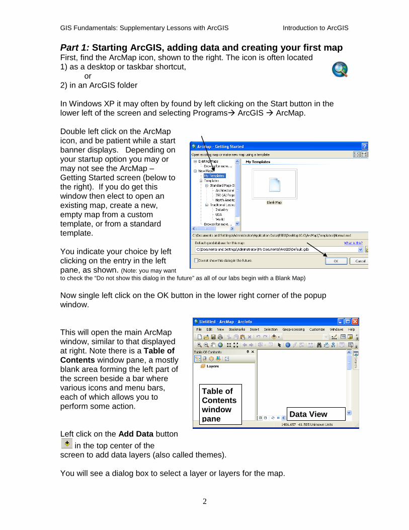
Part 1: Starting ArcGIS, adding data and creating your first map First, find the ArcMap icon, shown to the right. The icon is often located 1) as a desktop or taskbar shortcut, or 2) in an ArcGIS folder In Windows XP it may often by found by left clicking on the Start button in the lower left of the screen and selecting Programs ArcGIS ArcMap. Double left click on the ArcMap icon, and be patient while a start banner displays. Depending on your startup option you may or may not see the ArcMap – Getting Started screen (below to the right). If you do get this window then elect to open an existing map, create a new, empty map from a custom template, or from a standard template. You indicate your choice by left clicking on the entry in the left pane, as shown. (Note: you may want to check the “Do not show this dialog in the future” as all of our labs begin with a Blank Map) Now single left click on the OK button in the lower right corner of the popup window. This will open the main ArcMap window, similar to that displayed at right. Note there is a Table of Contents window pane, a mostly blank area forming the left part of the screen beside a bar where various icons and menu bars, each of which allows you to perform some action. Left click on the Add Data button

in the top center of the screen to add data layers (also called themes). You will see a dialog box to select a layer or layers for the map.

Data View

Table of Contents window pane


3

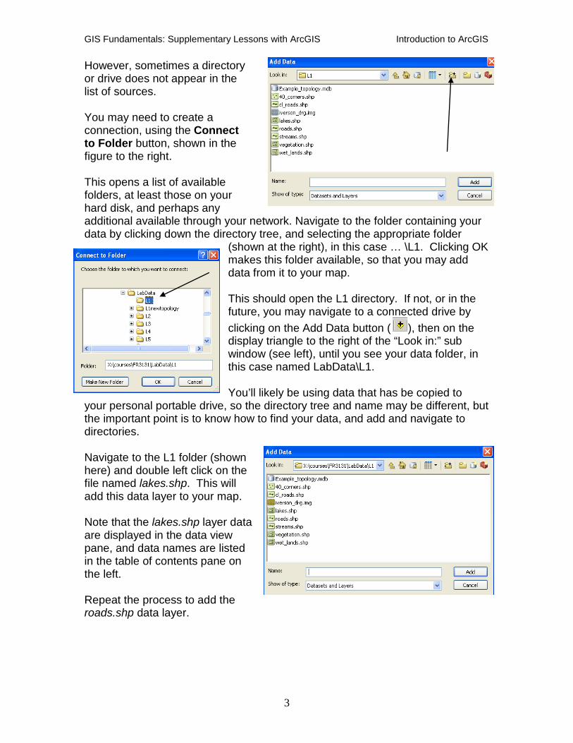
However, sometimes a directory or drive does not appear in the list of sources. You may need to create a connection, using the Connect to Folder button, shown in the figure to the right. This opens a list of available folders, at least those on your hard disk, and perhaps any additional available through your network. Navigate to the folder containing your data by clicking down the directory tree, and selecting the appropriate folder

(shown at the right), in this case … \L1. Clicking OK makes this folder available, so that you may add data from it to your map. This should open the L1 directory. If not, or in the future, you may navigate to a connected drive by clicking on the Add Data button ( ), then on the display triangle to the right of the “Look in:” sub window (see left), until you see your data folder, in this case named LabData\L1. You’ll likely be using data that has be copied to

your personal portable drive, so the directory tree and name may be different, but the important point is to know how to find your data, and add and navigate to directories. Navigate to the L1 folder (shown here) and double left click on the file named lakes.shp. This will add this data layer to your map. Note that the lakes.shp layer data are displayed in the data view pane, and data names are listed in the table of contents pane on the left. Repeat the process to add the roads.shp data layer.


4

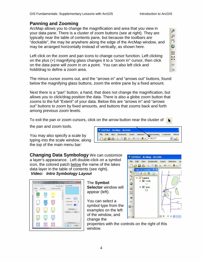
Panning and Zooming ArcMap allows you to change the magnification and area that you view in your data pane. There is a cluster of zoom buttons (see at right). They are typically near the table of contents pane, but because the toolbars are “dockable”, the may be anywhere along the edge of the ArcMap window, and may be arranged horizontally instead of vertically, as shown here. Left click on the zoom and pan icons to change cursor function. Left clicking on the plus (+) magnifying glass changes it to a “zoom in” cursor, then click on the data pane will zoom in on a point. You can also left click and hold/drag to define a zoom area. The minus cursor zooms out, and the “arrows in” and “arrows out” buttons, found below the magnifying glass buttons, zoom the entire pane by a fixed amount. Next there is a “pan” button, a hand, that does not change the magnification, but allows you to click/drag position the data. There is also a globe zoom button that zooms to the full “Extent” of your data. Below this are “arrows in” and “arrows out” buttons to zoom by fixed amounts, and buttons that zooms back and forth among previous zoom levels. To exit the pan or zoom cursors, click on the arrow button near the cluster of

the pan and zoom tools. You may also specify a scale by typing into the scale window, along the top of the main menu bar: Changing Data Symbology We can customize a layer’s appearance. Left double-click on a symbol icon, the colored patch below the name of the lakes data layer in the table of contents (see right). Video: Intro Symbology Layout

The Symbol Selector window will appear (left). You can select a symbol type from the examples on the left of the window, and change the properties with the controls on the right of this window.


5

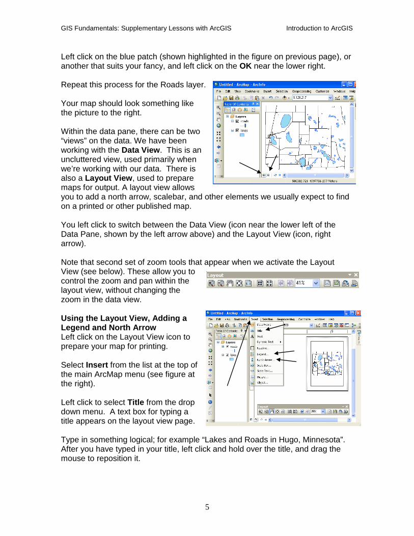
Left click on the blue patch (shown highlighted in the figure on previous page), or another that suits your fancy, and left click on the OK near the lower right. Repeat this process for the Roads layer. Your map should look something like the picture to the right. Within the data pane, there can be two “views” on the data. We have been working with the Data View. This is an uncluttered view, used primarily when we’re working with our data. There is also a Layout View, used to prepare maps for output. A layout view allows you to add a north arrow, scalebar, and other elements we usually expect to find on a printed or other published map. You left click to switch between the Data View (icon near the lower left of the Data Pane, shown by the left arrow above) and the Layout View (icon, right arrow). Note that second set of zoom tools that appear when we activate the Layout View (see below). These allow you to control the zoom and pan within the layout view, without changing the zoom in the data view. Using the Layout View, Adding a Legend and North Arrow Left click on the Layout View icon to prepare your map for printing. Select Insert from the list at the top of the main ArcMap menu (see figure at the right). Left click to select Title from the drop down menu. A text box for typing a title appears on the layout view page. Type in something logical; for example “Lakes and Roads in Hugo, Minnesota”. After you have typed in your title, left click and hold over the title, and drag the mouse to reposition it.


6

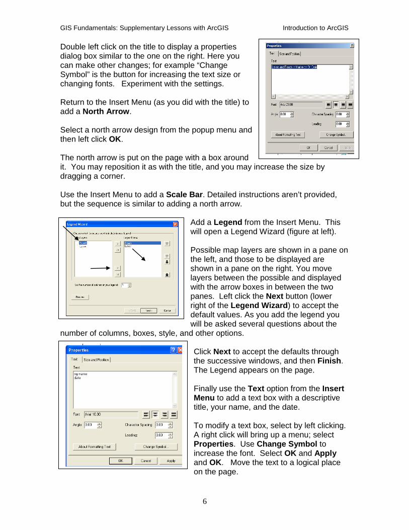
Double left click on the title to display a properties dialog box similar to the one on the right. Here you can make other changes; for example “Change Symbol” is the button for increasing the text size or changing fonts. Experiment with the settings. Return to the Insert Menu (as you did with the title) to add a North Arrow. Select a north arrow design from the popup menu and then left click OK. The north arrow is put on the page with a box around it. You may reposition it as with the title, and you may increase the size by dragging a corner. Use the Insert Menu to add a Scale Bar. Detailed instructions aren’t provided, but the sequence is similar to adding a north arrow.

Add a Legend from the Insert Menu. This will open a Legend Wizard (figure at left). Possible map layers are shown in a pane on the left, and those to be displayed are shown in a pane on the right. You move layers between the possible and displayed with the arrow boxes in between the two panes. Left click the Next button (lower right of the Legend Wizard) to accept the default values. As you add the legend you will be asked several questions about the

number of columns, boxes, style, and other options. Click Next to accept the defaults through the successive windows, and then Finish. The Legend appears on the page. Finally use the Text option from the Insert Menu to add a text box with a descriptive title, your name, and the date. To modify a text box, select by left clicking. A right click will bring up a menu; select Properties. Use Change Symbol to increase the font. Select OK and Apply and OK. Move the text to a logical place on the page.


7

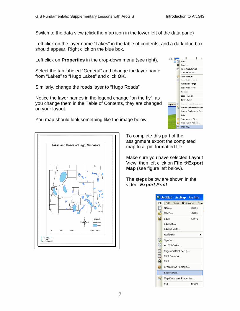
Switch to the data view (click the map icon in the lower left of the data pane) Left click on the layer name “Lakes” in the table of contents, and a dark blue box should appear. Right click on the blue box. Left click on Properties in the drop-down menu (see right). Select the tab labeled “General” and change the layer name from “Lakes” to “Hugo Lakes” and click OK. Similarly, change the roads layer to “Hugo Roads” Notice the layer names in the legend change “on the fly”, as you change them in the Table of Contents, they are changed on your layout. You map should look something like the image below.

To complete this part of the assignment export the completed map to a .pdf formatted file. Make sure you have selected Layout View, then left click on File Export Map (see figure left below). The steps below are shown in the video: Export Print


8

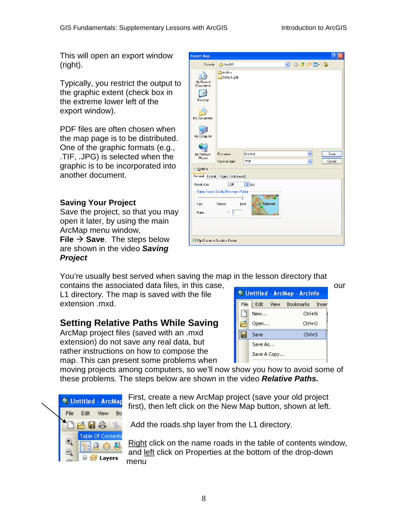
This will open an export window (right). Typically, you restrict the output to the graphic extent (check box in the extreme lower left of the export window). PDF files are often chosen when the map page is to be distributed. One of the graphic formats (e.g., .TIF, .JPG) is selected when the graphic is to be incorporated into another document. Saving Your Project Save the project, so that you may open it later, by using the main ArcMap menu window, File Save. The steps below are shown in the video Saving Project You’re usually best served when saving the map in the lesson directory that contains the associated data files, in this case, our L1 directory. The map is saved with the file extension .mxd. Setting Relative Paths While Saving ArcMap project files (saved with an .mxd extension) do not save any real data, but rather instructions on how to compose the map. This can present some problems when moving projects among computers, so we’ll now show you how to avoid some of these problems. The steps below are shown in the video Relative Paths.

First, create a new ArcMap project (save your old project first), then left click on the New Map button, shown at left. Add the roads.shp layer from the L1 directory. Right click on the name roads in the table of contents window, and left click on Properties at the bottom of the drop-down menu


9

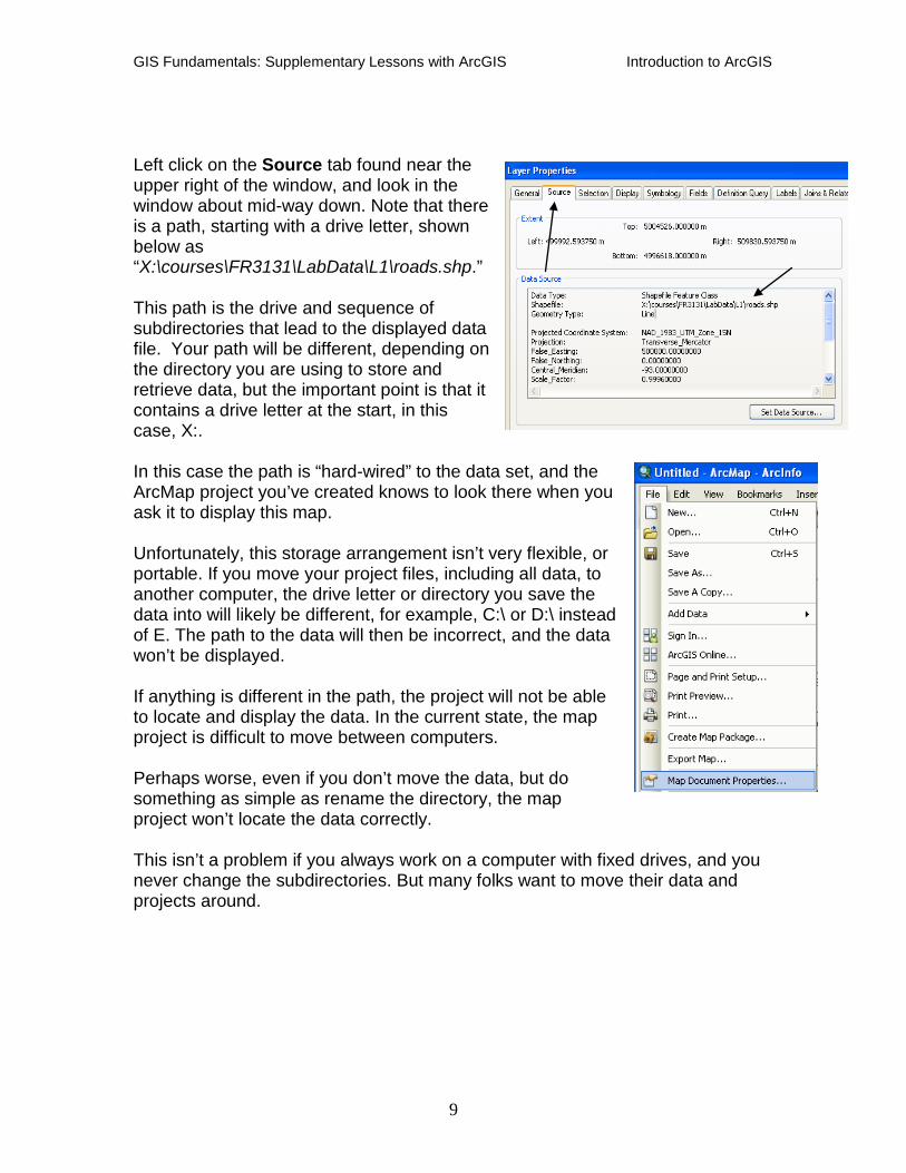
Left click on the Source tab found near the upper right of the window, and look in the window about mid-way down. Note that there is a path, starting with a drive letter, shown below as “X:\courses\FR3131\LabData\L1\roads.shp.” This path is the drive and sequence of subdirectories that lead to the displayed data file. Your path will be different, depending on the directory you are using to store and retrieve data, but the important point is that it contains a drive letter at the start, in this case, X:. In this case the path is “hard-wired” to the data set, and the ArcMap project you’ve created knows to look there when you ask it to display this map. Unfortunately, this storage arrangement isn’t very flexible, or portable. If you move your project files, including all data, to another computer, the drive letter or directory you save the data into will likely be different, for example, C:\ or D:\ instead of E. The path to the data will then be incorrect, and the data won’t be displayed. If anything is different in the path, the project will not be able to locate and display the data. In the current state, the map project is difficult to move between computers. Perhaps worse, even if you don’t move the data, but do something as simple as rename the directory, the map project won’t locate the data correctly. This isn’t a problem if you always work on a computer with fixed drives, and you never change the subdirectories. But many folks want to move their data and projects around.


10

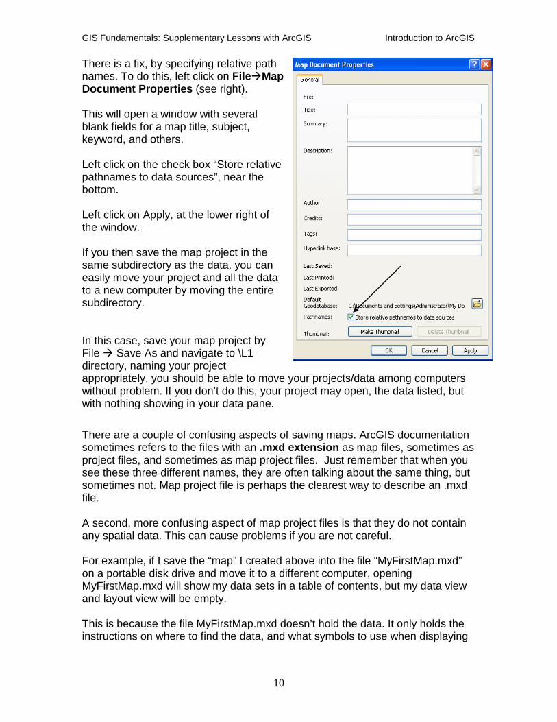
There is a fix, by specifying relative path names. To do this, left click on FileMap Document Properties (see right). This will open a window with several blank fields for a map title, subject, keyword, and others. Left click on the check box “Store relative pathnames to data sources”, near the bottom. Left click on Apply, at the lower right of the window. If you then save the map project in the same subdirectory as the data, you can easily move your project and all the data to a new computer by moving the entire subdirectory. In this case, save your map project by File Save As and navigate to \L1 directory, naming your project appropriately, you should be able to move your projects/data among computers without problem. If you don’t do this, your project may open, the data listed, but with nothing showing in your data pane. There are a couple of confusing aspects of saving maps. ArcGIS documentation sometimes refers to the files with an .mxd extension as map files, sometimes as project files, and sometimes as map project files. Just remember that when you see these three different names, they are often talking about the same thing, but sometimes not. Map project file is perhaps the clearest way to describe an .mxd file. A second, more confusing aspect of map project files is that they do not contain any spatial data. This can cause problems if you are not careful. For example, if I save the “map” I created above into the file “MyFirstMap.mxd” on a portable disk drive and move it to a different computer, opening MyFirstMap.mxd will show my data sets in a table of contents, but my data view and layout view will be empty. This is because the file MyFirstMap.mxd doesn’t hold the data. It only holds the instructions on where to find the data, and what symbols to use when displaying


11

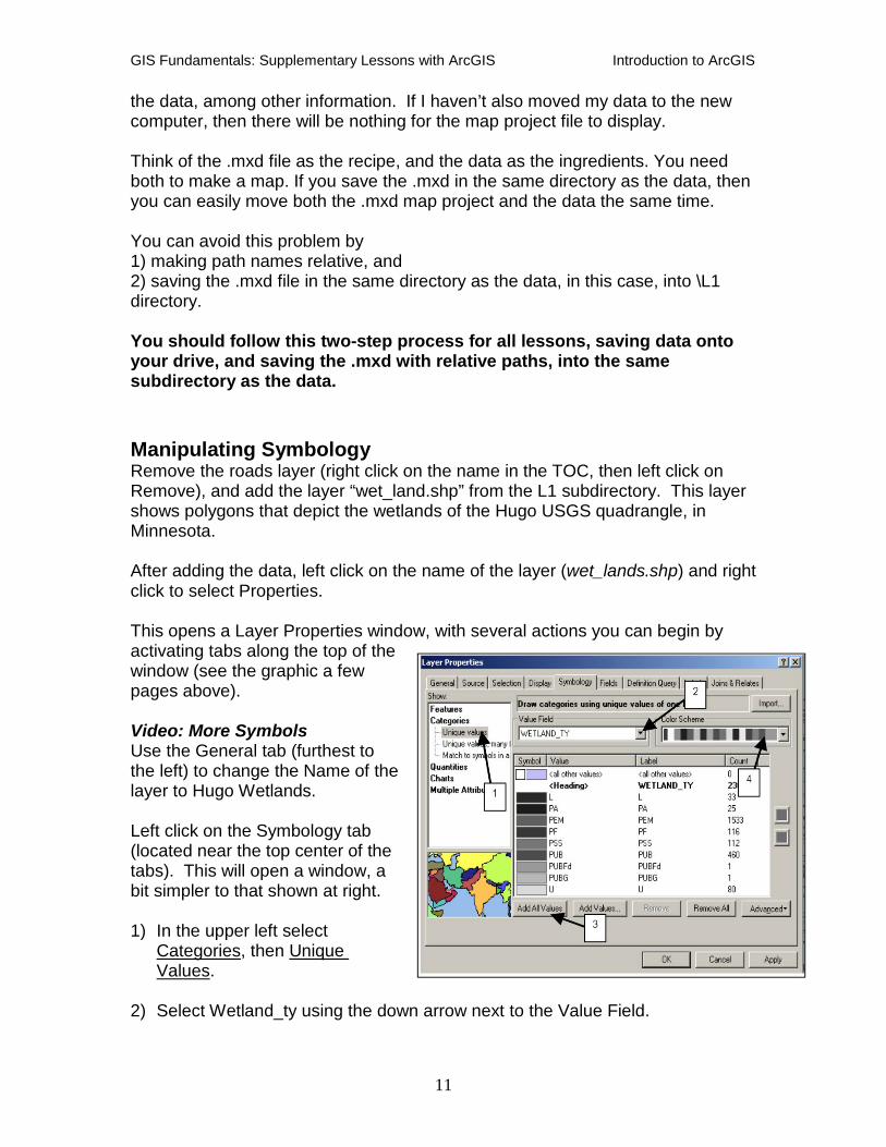
the data, among other information. If I haven’t also moved my data to the new computer, then there will be nothing for the map project file to display. Think of the .mxd file as the recipe, and the data as the ingredients. You need both to make a map. If you save the .mxd in the same directory as the data, then you can easily move both the .mxd map project and the data the same time. You can avoid this problem by 1) making path names relative, and 2) saving the .mxd file in the same directory as the data, in this case, into \L1 directory. You should follow this two-step process for all lessons, saving data onto your drive, and saving the .mxd with relative paths, into the same subdirectory as the data. Manipulating Symbology Remove the roads layer (right click on the name in the TOC, then left click on Remove), and add the layer “wet_land.shp” from the L1 subdirectory. This layer shows polygons that depict the wetlands of the Hugo USGS quadrangle, in Minnesota. After adding the data, left click on the name of the layer (wet_lands.shp) and right click to select Properties. This opens a Layer Properties window, with several actions you can begin by activating tabs along the top of the window (see the graphic a few pages above). Video: More Symbols Use the General tab (furthest to the left) to change the Name of the layer to Hugo Wetlands. Left click on the Symbology tab (located near the top center of the tabs). This will open a window, a bit simpler to that shown at right. 1) In the upper left select

Categories, then Unique Values.

2) Select Wetland_ty using the down arrow next to the Value Field.


12

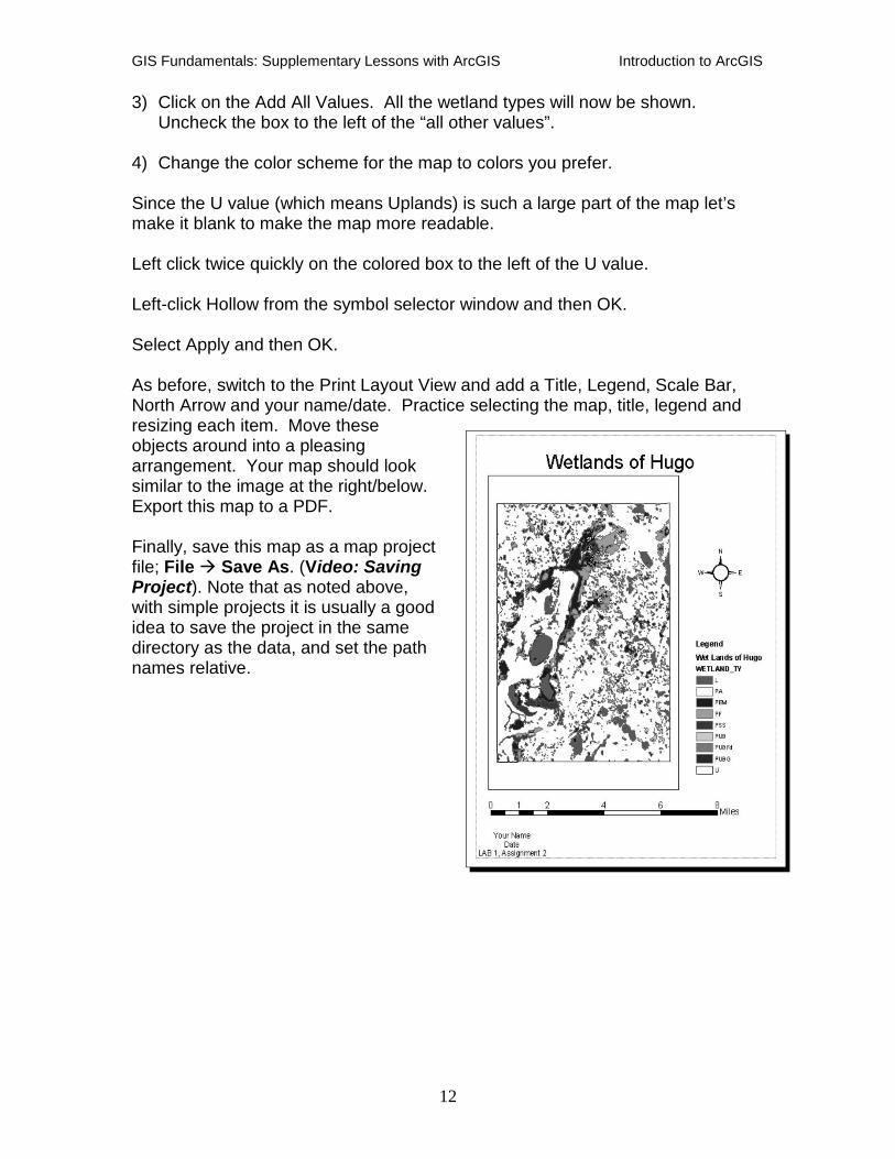
3) Click on the Add All Values. All the wetland types will now be shown. Uncheck the box to the left of the “all other values”.

4) Change the color scheme for the map to colors you prefer. Since the U value (which means Uplands) is such a large part of the map let’s make it blank to make the map more readable. Left click twice quickly on the colored box to the left of the U value. Left-click Hollow from the symbol selector window and then OK. Select Apply and then OK. As before, switch to the Print Layout View and add a Title, Legend, Scale Bar, North Arrow and your name/date. Practice selecting the map, title, legend and resizing each item. Move these objects around into a pleasing arrangement. Your map should look similar to the image at the right/below. Export this map to a PDF. Finally, save this map as a map project file; File Save As. (Video: Saving Project). Note that as noted above, with simple projects it is usually a good idea to save the project in the same directory as the data, and set the path names relative.


13

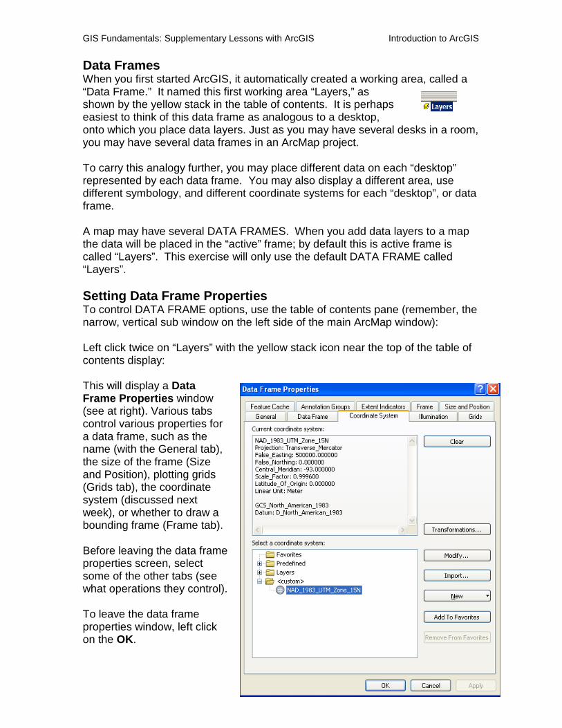
Data Frames When you first started ArcGIS, it automatically created a working area, called a “Data Frame.” It named this first working area “Layers,” as shown by the yellow stack in the table of contents. It is perhaps easiest to think of this data frame as analogous to a desktop, onto which you place data layers. Just as you may have several desks in a room, you may have several data frames in an ArcMap project. To carry this analogy further, you may place different data on each “desktop” represented by each data frame. You may also display a different area, use different symbology, and different coordinate systems for each “desktop”, or data frame. A map may have several DATA FRAMES. When you add data layers to a map the data will be placed in the “active” frame; by default this is active frame is called “Layers”. This exercise will only use the default DATA FRAME called “Layers”. Setting Data Frame Properties To control DATA FRAME options, use the table of contents pane (remember, the narrow, vertical sub window on the left side of the main ArcMap window): Left click twice on “Layers” with the yellow stack icon near the top of the table of contents display: This will display a Data Frame Properties window (see at right). Various tabs control various properties for a data frame, such as the name (with the General tab), the size of the frame (Size and Position), plotting grids (Grids tab), the coordinate system (discussed next week), or whether to draw a bounding frame (Frame tab). Before leaving the data frame properties screen, select some of the other tabs (see what operations they control). To leave the data frame properties window, left click on the OK.


14

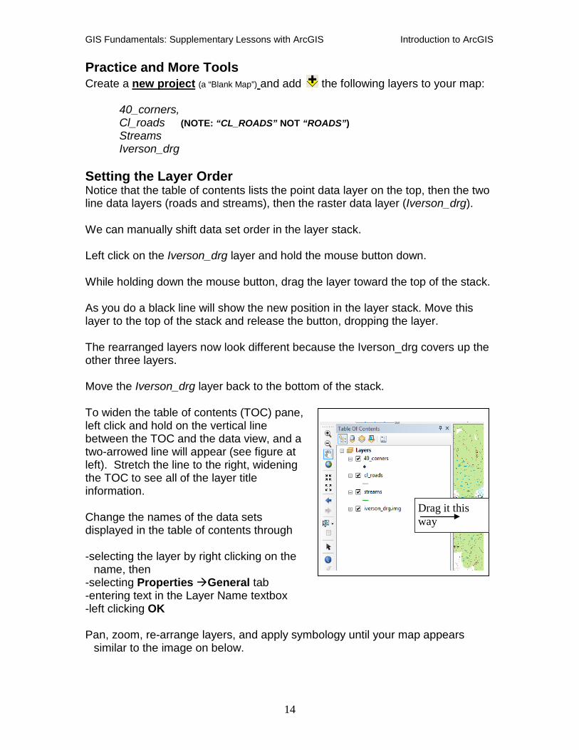
Practice and More Tools Create a new project (a “Blank Map”) and add the following layers to your map: 40_corners, Cl_roads (NOTE: “CL_ROADS” NOT “ROADS”) Streams Iverson_drg Setting the Layer Order Notice that the table of contents lists the point data layer on the top, then the two line data layers (roads and streams), then the raster data layer (Iverson_drg). We can manually shift data set order in the layer stack. Left click on the Iverson_drg layer and hold the mouse button down. While holding down the mouse button, drag the layer toward the top of the stack. As you do a black line will show the new position in the layer stack. Move this layer to the top of the stack and release the button, dropping the layer. The rearranged layers now look different because the Iverson_drg covers up the other three layers. Move the Iverson_drg layer back to the bottom of the stack. To widen the table of contents (TOC) pane, left click and hold on the vertical line between the TOC and the data view, and a two-arrowed line will appear (see figure at left). Stretch the line to the right, widening the TOC to see all of the layer title information. Change the names of the data sets displayed in the table of contents through -selecting the layer by right clicking on the

name, then -selecting Properties General tab -entering text in the Layer Name textbox -left clicking OK Pan, zoom, re-arrange layers, and apply symbology until your map appears

similar to the image on below.

Drag it this way


15

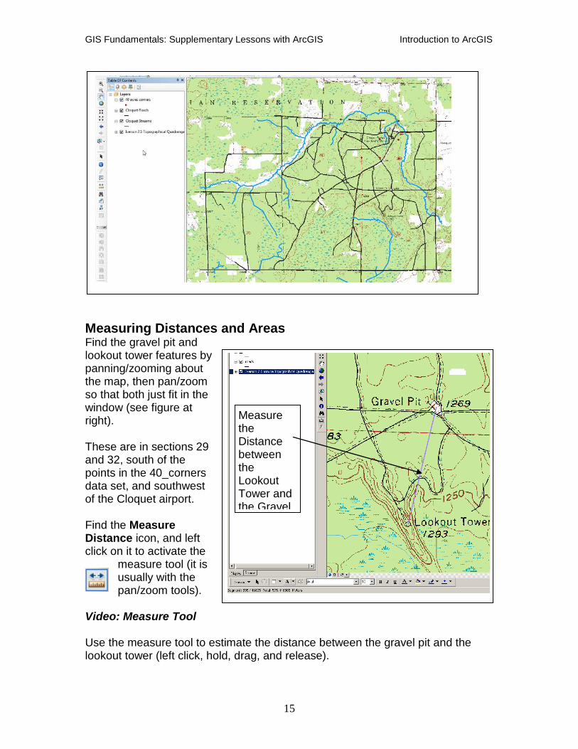
Measuring Distances and Areas Find the gravel pit and lookout tower features by panning/zooming about the map, then pan/zoom so that both just fit in the window (see figure at right). These are in sections 29 and 32, south of the points in the 40_corners data set, and southwest of the Cloquet airport. Find the Measure Distance icon, and left click on it to activate the

measure tool (it is usually with the pan/zoom tools).

Video: Measure Tool Use the measure tool to estimate the distance between the gravel pit and the lookout tower (left click, hold, drag, and release).

Measure the Distance between the Lookout Tower and the Gravel


16

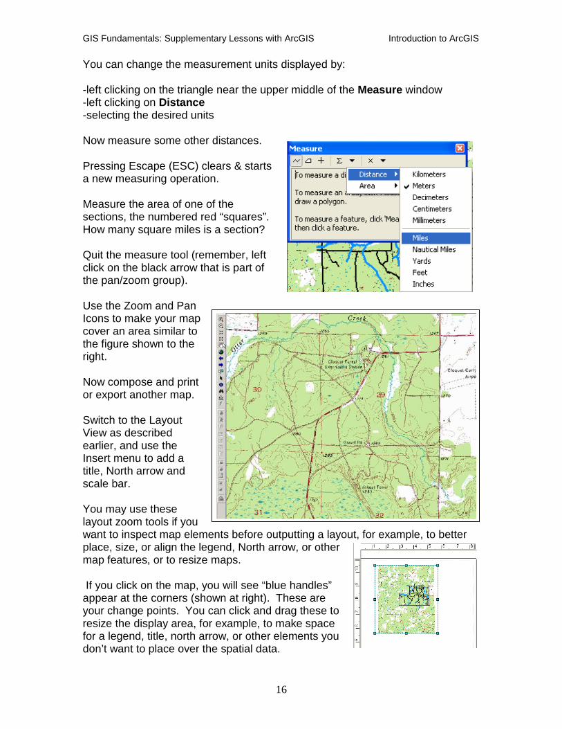
You can change the measurement units displayed by: -left clicking on the triangle near the upper middle of the Measure window -left clicking on Distance -selecting the desired units Now measure some other distances. Pressing Escape (ESC) clears & starts a new measuring operation. Measure the area of one of the sections, the numbered red “squares”. How many square miles is a section? Quit the measure tool (remember, left click on the black arrow that is part of the pan/zoom group). Use the Zoom and Pan Icons to make your map cover an area similar to the figure shown to the right. Now compose and print or export another map. Switch to the Layout View as described earlier, and use the Insert menu to add a title, North arrow and scale bar. You may use these layout zoom tools if you want to inspect map elements before outputting a layout, for example, to better place, size, or align the legend, North arrow, or other map features, or to resize maps. If you click on the map, you will see “blue handles” appear at the corners (shown at right). These are your change points. You can click and drag these to resize the display area, for example, to make space for a legend, title, north arrow, or other elements you don’t want to place over the spatial data.


17

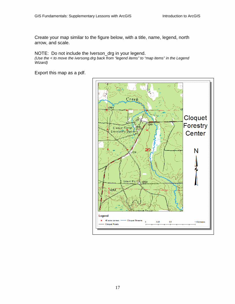
Create your map similar to the figure below, with a title, name, legend, north arrow, and scale. NOTE: Do not include the Iverson_drg in your legend. (Use the < to move the iversong.drg back from “legend items” to “map items” in the Legend Wizard) Export this map as a pdf.


18

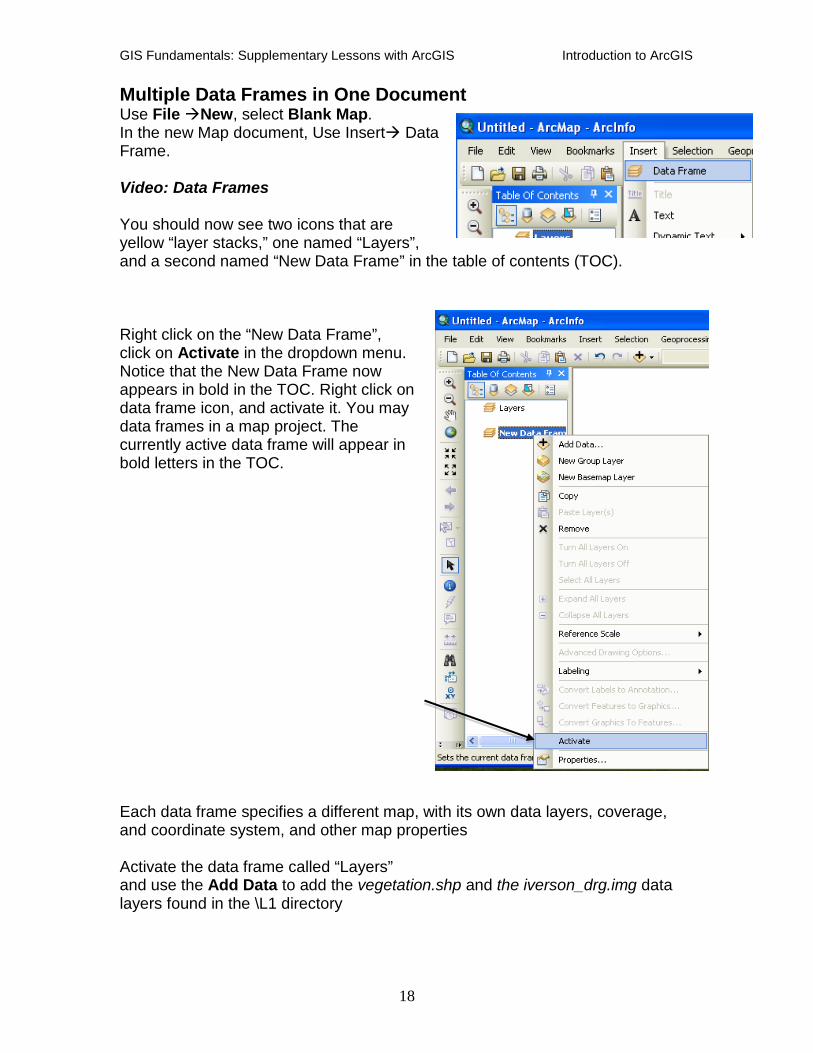
Multiple Data Frames in One Document Use File New, select Blank Map. In the new Map document, Use Insert Data Frame. Video: Data Frames You should now see two icons that are yellow “layer stacks,” one named “Layers”, and a second named “New Data Frame” in the table of contents (TOC). Right click on the “New Data Frame”, click on Activate in the dropdown menu. Notice that the New Data Frame now appears in bold in the TOC. Right click on the “Layers” data frame icon, and activate it. You may have several data frames in a map project. The currently active data frame will appear in bold letters in the TOC. Each data frame specifies a different map, with its own data layers, coverage, and coordinate system, and other map properties Activate the data frame called “Layers” and use the Add Data to add the vegetation.shp and the iverson_drg.img data layers found in the \L1 directory


19

Right click over the data frame named “Layers” in the table of contents From the drop-down menu, select Properties (at the very bottom, just below Activate) This should display a Data Frame Properties menu.

Select the General tab. Specify a Name of “Inset”. Then left click on Apply and OK

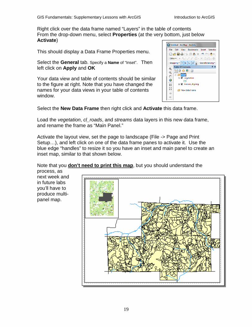
Your data view and table of contents should be similar to the figure at right. Note that you have changed the names for your data views in your table of contents window. Select the New Data Frame then right click and Activate this data frame. Load the vegetation, cl_roads, and streams data layers in this new data frame, and rename the frame as “Main Panel.” Activate the layout view, set the page to landscape (File -> Page and Print Setup…), and left click on one of the data frame panes to activate it. Use the blue edge “handles” to resize it so you have an inset and main panel to create an inset map, similar to that shown below. Note that you don’t need to print this map, but you should understand the process, as next week and in future labs you’ll have to produce multi-panel map.


20

Part 2: GeoDatabases You may wonder about the data layers you have just used for your two maps, Lakes, Roads, and wet_land. These layers are shapefiles, a special file type defined by ESRI for storing spatial data. Shapefiles are a group of files that share a file name but have different extensions, such as .shp or .dbf or .prj. ESRI subsequently created a more complex data structure, called a GeoDatabase. You typically create the GeoDatabases (or the simpler/older shapefiles) by left-clicking on the catalog tool:

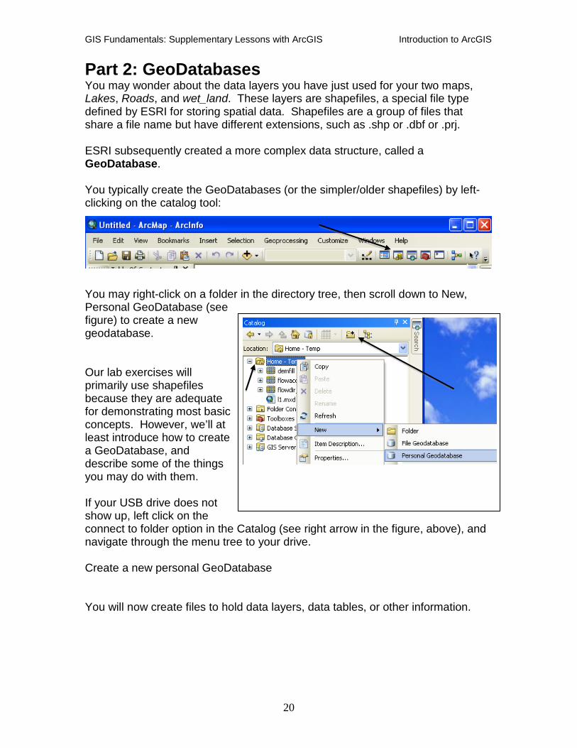
You may right-click on a folder in the directory tree, then scroll down to New, Personal GeoDatabase (see figure) to create a new geodatabase. Our lab exercises will primarily use shapefiles because they are adequate for demonstrating most basic concepts. However, we’ll at least introduce how to create a GeoDatabase, and describe some of the things you may do with them. If your USB drive does not show up, left click on the connect to folder option in the Catalog (see right arrow in the figure, above), and navigate through the menu tree to your drive. Create a new personal GeoDatabase You will now create files to hold data layers, data tables, or other information.


21

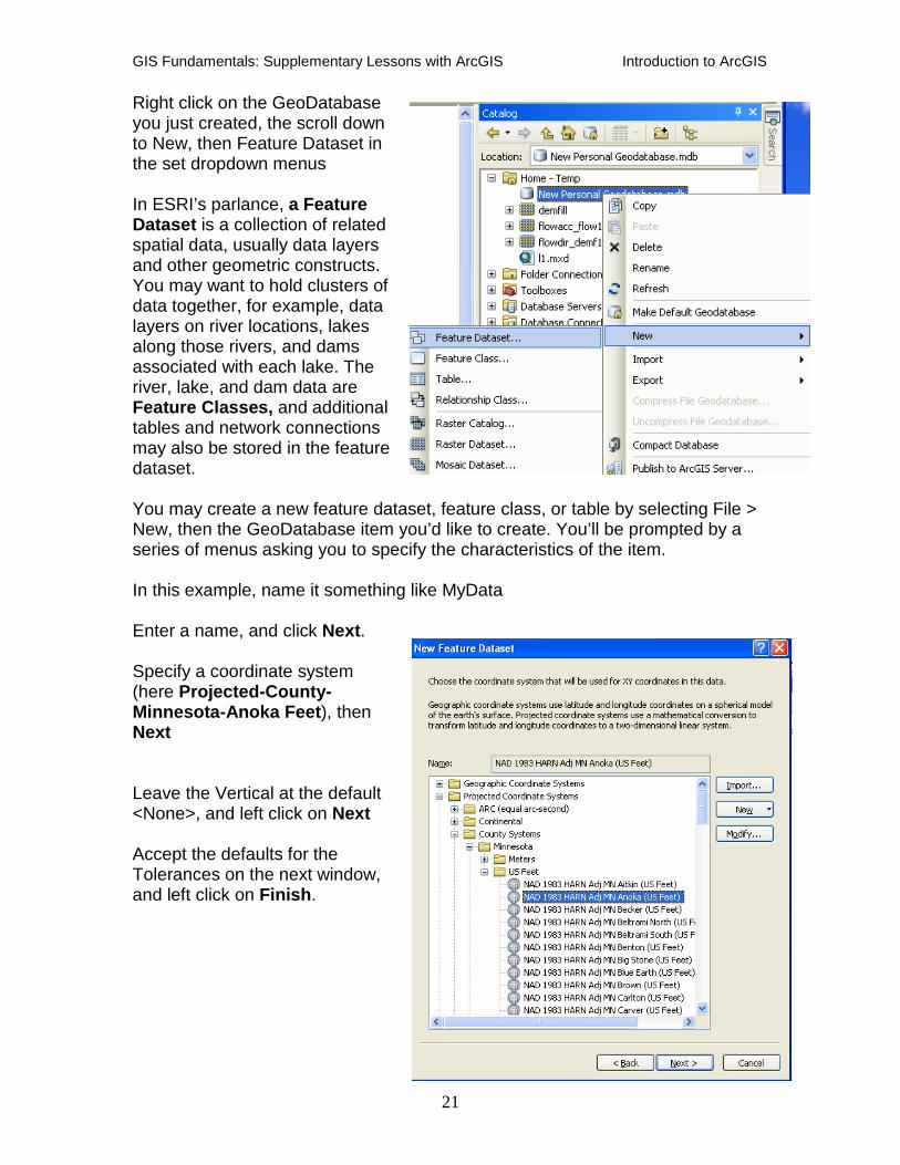
Right click on the GeoDatabase you just created, the scroll down to New, then Feature Dataset in the set dropdown menus In ESRI’s parlance, a Feature Dataset is a collection of related spatial data, usually data layers and other geometric constructs. You may want to hold clusters of data together, for example, data layers on river locations, lakes along those rivers, and dams associated with each lake. The river, lake, and dam data are Feature Classes, and additional tables and network connections may also be stored in the feature dataset. You may create a new feature dataset, feature class, or table by selecting File > New, then the GeoDatabase item you’d like to create. You’ll be prompted by a series of menus asking you to specify the characteristics of the item. In this example, name it something like MyData Enter a name, and click Next. Specify a coordinate system (here Projected-County-Minnesota-Anoka Feet), then Next Leave the Vertical at the default <None>, and left click on Next Accept the defaults for the Tolerances on the next window, and left click on Finish.


22

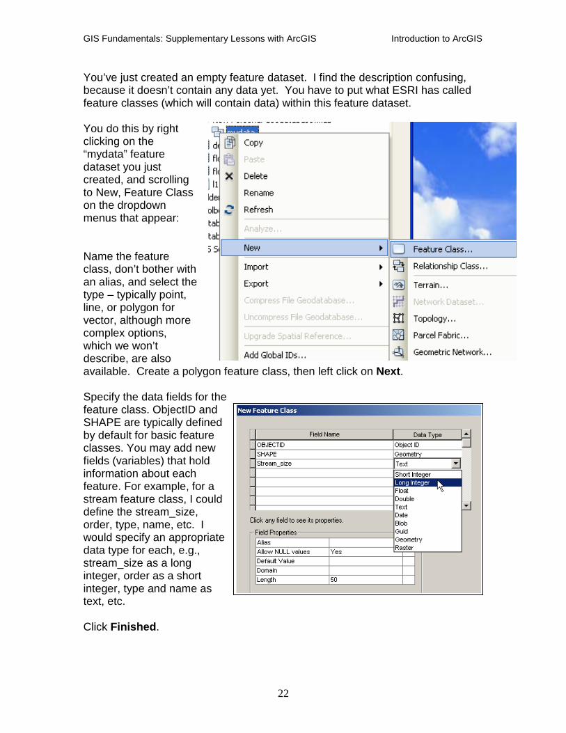
You’ve just created an empty feature dataset. I find the description confusing, because it doesn’t contain any data yet. You have to put what ESRI has called feature classes (which will contain data) within this feature dataset. You do this by right clicking on the “mydata” feature dataset you just created, and scrolling to New, Feature Class on the dropdown menus that appear: Name the feature class, don’t bother with an alias, and select the type – typically point, line, or polygon for vector, although more complex options, which we won’t describe, are also available. Create a polygon feature class, then left click on Next. Specify the data fields for the feature class. ObjectID and SHAPE are typically defined by default for basic feature classes. You may add new fields (variables) that hold information about each feature. For example, for a stream feature class, I could define the stream_size, order, type, name, etc. I would specify an appropriate data type for each, e.g., stream_size as a long integer, order as a short integer, type and name as text, etc. Click Finished.


23

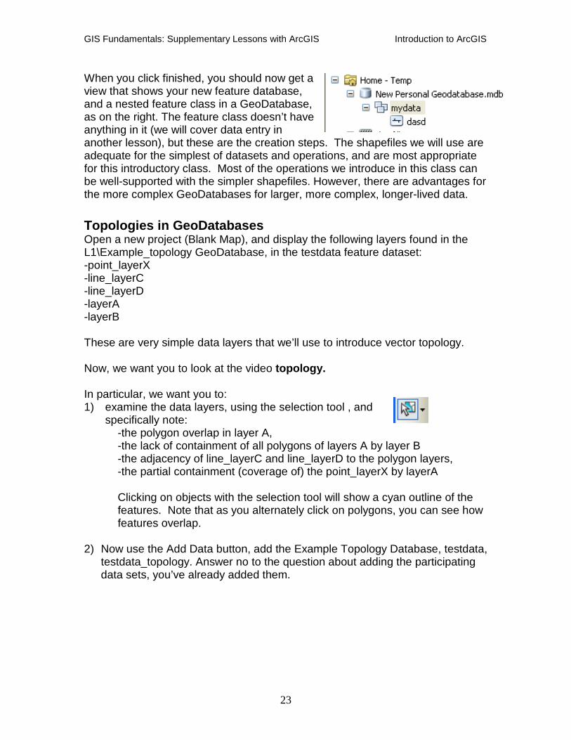
When you click finished, you should now get a view that shows your new feature database, and a nested feature class in a GeoDatabase, as on the right. The feature class doesn’t have anything in it (we will cover data entry in another lesson), but these are the creation steps. The shapefiles we will use are adequate for the simplest of datasets and operations, and are most appropriate for this introductory class. Most of the operations we introduce in this class can be well-supported with the simpler shapefiles. However, there are advantages for the more complex GeoDatabases for larger, more complex, longer-lived data. Topologies in GeoDatabases Open a new project (Blank Map), and display the following layers found in the L1\Example_topology GeoDatabase, in the testdata feature dataset: -point_layerX -line_layerC -line_layerD -layerA -layerB These are very simple data layers that we’ll use to introduce vector topology. Now, we want you to look at the video topology. In particular, we want you to: 1) examine the data layers, using the selection tool , and

specifically note: -the polygon overlap in layer A, -the lack of containment of all polygons of layers A by layer B -the adjacency of line_layerC and line_layerD to the polygon layers, -the partial containment (coverage of) the point_layerX by layerA Clicking on objects with the selection tool will show a cyan outline of the features. Note that as you alternately click on polygons, you can see how features overlap.

2) Now use the Add Data button, add the Example Topology Database, testdata,

testdata_topology. Answer no to the question about adding the participating data sets, you’ve already added them.


24

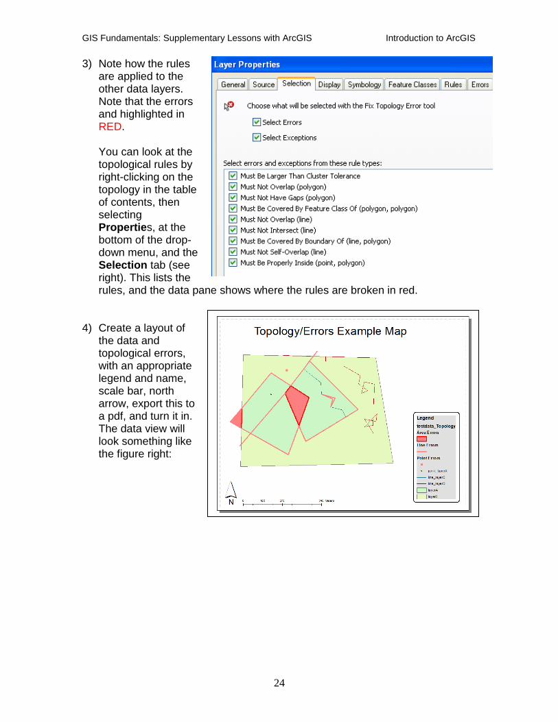
3) Note how the rules are applied to the other data layers. Note that the errors and highlighted in RED. You can look at the topological rules by right-clicking on the topology in the table of contents, then selecting Properties, at the bottom of the drop-down menu, and the Selection tab (see right). This lists the rules, and the data pane shows where the rules are broken in red.

4) Create a layout of the data and topological errors, with an appropriate legend and name, scale bar, north arrow, export this to a pdf, and turn it in. The data view will look something like the figure right:

Documents

Lesson 1: Introduction to ArcGIS - Geology Departmentgeology.wlu.edu/harbor/geol260/tutor/bolstad/Lesson1_Arc10.pdf · GIS Fundamentals: Supplementary Lessons with ArcGIS Introduction