LEXANDER UBCEK NIVERSITY OF RENCIN

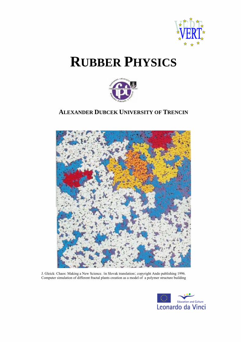
RUBBER PHYSICS

ALEXANDER DUBCEK UNIVERSITY OF TRENCIN

J. Gleick: Chaos: Making a New Science. /in Slovak translation/, copyright Ando publishing 1996. Computer simulation of different fractal plants creation as a model of a polymer structure building

SUMMARY

The module ‘Physics of polymers’ is the field of physics associated to the study of polymers, understanding of the mechanical, physical, electrical and thermodynamic properties of polymeric materials. Current areas of focus include structural and mechanical behavior of networks, segmental relaxation and the glass transition, miscible polymer blends, and polymer-based composites. Polymer physics is part of the wider field of polymer science. All of these aspects are discussed in this module, which consists therefore of the following seven parts:

• Structure of polymers & Physical and phase states of polymers • Mechanical properties of solid state polymers • Payene effect & Viscosity and mechanical properties of viscous and

viscoelastic materials & Fracture properties of polymers • Models of viscoelastic behavior of materials • Selected physical properties of polymeric materials • Electrical properties of polymers • Physical Processes Influencing Surface Contact of Two Materials

The first sub-module discusses polymer materials; their basic structure units, that is good for better understanding of distinctiveness of polymers as materials, it is purposeful to consider the conception of the hierarchic disposition of macromolecular materials. We have tried to explain the constitutional unit, there are shown here some types of polymer chains. Density of cohesive energy is explained here and we introduce for polymers derived quantity, namely the parameter of solubility and geometry of polymer chain. The aim of the second part of the first sub-module that is called physical and phase states of polymers explains basic states for polymers as gaseous, liquid and solid state, structural and phase transformation that takes place in them. Readers can obtain iformation about 14 different crystal lattices, called Bravais Lattices. It describes also phenomenological description of glassy state. Next there is phase transitions described as transition of state, transformation of amorphous substance into crystalline and vice versa, or transformation of one crystalline system into another. Glass transition temperature defined as temperature, at which bend or discontinuity occurs on dependence of specific volume on temperature. There are deffined several methods for the determination of glass transition temperature.

The second sub-model deals with a description of deformation of solid elastic materials as well as to set up phenomenological values describing mechanical properties of these substances. We are going to learn about thermodynamic and microstructural aspects of the process of elastic deformation. Later on these concepts and knowledge will be generalized on polymers and rubber.

The third sub-module has three important parts. First part deals with a description of Payne effect and also with its physical description. The second one introduces the viscosity terms and viscoelastic behaviour of materials under loading. There is presented the terminology of complex physical parameters (modules), WLF transformations and results of rubber mixtures measurements and temperature dependence of viscosity. And the third one is devoted to the issue of the fracture attributes of polymeric materials, where fracture mechanics provides a methodology evaluating the structural integrity of components containing such defects, and demonstrating whether they are capable of continued, safe operation. The basic criterion in any fracture mechanics analysis is to prevent failure. You can find there information about the historical overview where are presented some approaches. In the fourth sub-model are introduced basic theoretical approaches describing viscoelastic behavior of materials. Readers will be familiared with basic models: Maxwell, Voigt and their combinations.

The fifth sub-model provide readers with a schematic review of results of measurements of selected physical quantities (especially mechanic and thermal) gained for various polymeric materials and rubber as well as their connection with theoretical background knowledge presented in previous parts. At the same time we are going to point out differences between physical properties of elastomers and polymers. The sixth sub-model introduces the specific resistivity and conductivity, dielectric properties of polymers, electrical stress of polymers and finally percolation threshold. The last one sub-model presents hysteretic attributes of viscoelastic materials in the process of their deformation. Some theoretical approaches of hysteresis explanation from the point of view of solids' contact are discussed. It also deals with gluing questions and adhesion at mutual contact of materials problems, as well as with theory of friction.

©Alexander Dubcek University of Trencin 2007 3

TABLE OF CONTENTS 1. Structure of polymers............................................................................................. 5

1.1. Basic information............................................................................................ 5 1.2. The density of the cohesive energy................................................................. 7 1.3. Geometry of polymer chains........................................................................... 9 1.4. Physical and phase states of polymers .......................................................... 13

1.4.1. Glassy state ............................................................................................ 13 1.4.2. Phase transitions .................................................................................... 15 1.4.3. Glass transition temperature .................................................................. 18

References:........................................................................................................... 24 2. ..................................................... 25Mechanical properties of solid state polymers

2.1. Description of deformation of solid elastic materials ................................... 25 2.2. Thermodynamic aspects of deformation....................................................... 35 References............................................................................................................ 37

3. ......... 38Viscosity and mechanical properties of viscous and viscoelastic materials3.1. Viscosity ....................................................................................................... 38 3.2. Time dependence of deformation ............................................................... 46 3.3. The temperature dependence of viscosity – micro structural view.......... 54 3.4. Thermodynamic aspects of viscous elastic and rubber deformation ....... 56 3.5. Payne effect................................................................................................... 60 3.6. Fracture properties of polymers .................................................................... 65 References........................................................................................................... 75

4. ....................................................... 77Models of viscoelastic behavior of materialsReferences:........................................................................................................... 83

5. ........................................... 85Selected physical properties of polymeric materialsReferences:......................................................................................................... 102

6. ....................................................................... 103Electrical properties of polymers6.1. Electrically Conductive Polymers............................................................... 103 6.2. Electrically Conductive Composites........................................................... 104 6.3. Influence of Force Field on Polymer Behaviour......................................... 106 6.4. Electrical Strength of Polymers .................................................................. 107 6.5. Dielectric Properties of Polymers ............................................................... 108 References......................................................................................................... 110

7. ................... 112Physical Processes Influencing Surface Contact of Two Materials7.1. Hysteresis.................................................................................................... 112

7.1.1. Theories of Hysteresis ......................................................................... 113 7.1.2. Unified Theory..................................................................................... 113 7.1.3. Relaxation Theory................................................................................ 115

7.2. Gluing and adhesion ................................................................................... 115 7.2.1. Adhesion as a surface problem ............................................................ 117 7.2.2. The Role of Adhesion at Dynamic Contact of Two Materials – Macroscopic and Molecular Understanding .................................................. 120 7.2.3. Ratio Theory ........................................................................................ 121 7.2.4. Mixed Theory ...................................................................................... 121

7.3. Friction........................................................................................................ 122 7.3.1. Friction as Dynamic Problem of Two Surfaces Contact ..................... 124

References......................................................................................................... 139


CHAPTER 1

Structure of polymers Objectives to achieve In this chapter are explained polymer materials; their basic structure units, density of cohesive energy and geometry of polymer chain and so on. The aim of this section is also to explain basic states for polymers, structural and phase transformation that takes place in them. It describes also phenomenological description of glassy state.

1.1. Basic information For better understanding of distinctiveness of polymers as materials, it is purposeful to consider the conception of the hierarchic disposition of macromolecular materials. Every condition, behaviour, or individual property is possible to be considered at least from three points of view:

- from the view of the structure and dynamic behaviour of an individual isolated molecule

- from the view of the change in behaviour of a macromolecule whose movements are limited by the closeness of other macromolecules

- and finally from the view of properties of polymeric material formed by large number of macromolecules which not only influence each other, but they can make various structural formations distinguishing from each other by thermodynamic parameters and certainly by numerous properties despite the identical chemical composition.

A polymer is formed by a large number of mutually connected “mers”, units, which are chemically identical. The repetition moment is typical for a polymer, when a defined grouping of atoms is repeated many times in an identical constellation. This repeating structure is called a structural, or a building unit, or according to the new nomenclature a constitutional unit that is defined as the smallest unit, whose repetition describes the regular polymer. In this process the constitutional unit doesn’t need to be necessarily identical with the structure coming out from a monomer. For example, the polymer for polyethyleneterephtalat is formed by poly-condensation of ethylene glycol and terephtalic acid, but the constitutional unit, that is, the repeating structure is:

– CH2 – CH2 – O – CO – C6H5 – CO – O – that is, a condensation product of two different individual reagents. A polymer is formed this way. From this point of view, every polymer is simultaneously a macromolecule, i.e. a molecule with a very large mass significantly exceeding a substance of so called low molecular materials. Molar


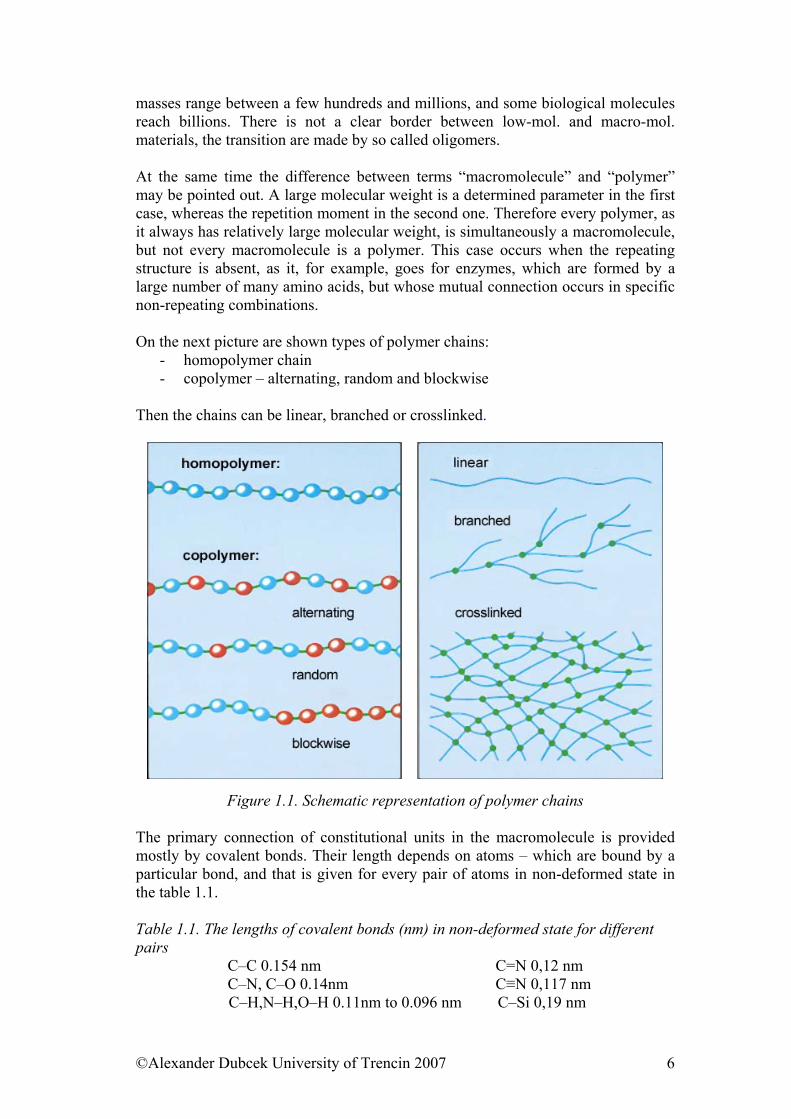
masses range between a few hundreds and millions, and some biological molecules reach billions. There is not a clear border between low-mol. and macro-mol. materials, the transition are made by so called oligomers. At the same time the difference between terms “macromolecule” and “polymer” may be pointed out. A large molecular weight is a determined parameter in the first case, whereas the repetition moment in the second one. Therefore every polymer, as it always has relatively large molecular weight, is simultaneously a macromolecule, but not every macromolecule is a polymer. This case occurs when the repeating structure is absent, as it, for example, goes for enzymes, which are formed by a large number of many amino acids, but whose mutual connection occurs in specific non-repeating combinations. On the next picture are shown types of polymer chains:

- homopolymer chain - copolymer – alternating, random and blockwise

Then the chains can be linear, branched or crosslinked.

Figure 1.1. Schematic representation of polymer chains The primary connection of constitutional units in the macromolecule is provided mostly by covalent bonds. Their length depends on atoms – which are bound by a particular bond, and that is given for every pair of atoms in non-deformed state in the table 1.1. Table 1.1. The lengths of covalent bonds (nm) in non-deformed state for different pairs

C–C 0.154 nm C=N 0,12 nm C–N, C–O 0.14nm C≡N 0,117 nm C–H,N–H,O–H 0.11nm to 0.096 nm C–Si 0,19 nm


C=C 0.13 nm Si–O 0,18 nm The solidness of the bond is formulated by dissipation bond energy, that is, by energy needed for disruption of the given bond. The dissipation energy of simple bonds is 250 - 400 kJ / mol, for multiple bonds it is 400 - 600 kJ / mol. It might be seen from the comparison that the dissipation energy of, for example, the second bond is lower than of a simple bond. It follows from this that a double bond is in comparison with a simple one more reactive. Also the fact, that the connection of atoms with a bond is sterically constant and that it might be characterized by so called a valence angle, is important for understanding of the structure of the macromolecular chain. These valence angles are given for individual types of bonds in the table 1.2. Table 1.2. Valence angles for different types of covalent bonds

H-C-H, C-C-C, C-O-C, C-N-C 105 - 113° C-C=C 125° C≡C 180° Si-O-Si 134°

It is important to realize for a discussion about geometry of polymeric chains that a free rotation of substituents around simple bonds is possible (producing different conformations), whereas a rotation of substituents around multiple bonds is not possible (configurational structure).

1.2. The density of the cohesive energy Apart from relatively solid primary bonds, that provide cohesion of each molecule in every material consisting of many molecules, there are much weaker secondary bonds. These bonds stand for cohesive power that affects molecules consisting of covalently bound atoms (van der Waals’s power). The molecules are 0.3 - 1 nm distant from each other and the energy needed for their disruption is less than 40 - 50 kJ/mol. The secondary bonds provide cohesion of whole material and present a power which molecules in a material are attracted mutually by. Their sum can be then considered as the rate of intermolecular cohesion. This energy significantly depends on the distance between molecules because the extent of intermolecular cohesion is proportional to the power of six of the distance between molecules. The solidness in low molecular materials is much lower than for primary bonds, and they come into high values only if they are polar, for example, acid-alkaline interactions, hydrogen bond, etc. To the contrary, the secondary bonds can be very solid for macromolecules, where the chain contains several thousands carbons, because the number of contacts is very large. Therefore, for example, butane is gas, whereas octane is already liquid, hydrocarbons with a chain of 20 – 30 carbons have a character of waxes with a low melting point, but, for example, linear polyethylene is resilient material where the secondary intermolecular bonds are more solid than the primary ones between atoms of carbons. Due to this fact the polymer is not


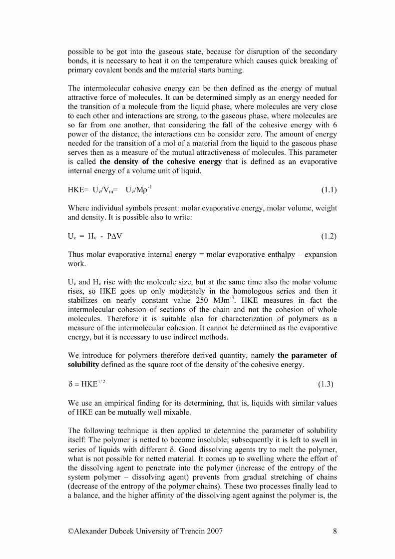
possible to be got into the gaseous state, because for disruption of the secondary bonds, it is necessary to heat it on the temperature which causes quick breaking of primary covalent bonds and the material starts burning. The intermolecular cohesive energy can be then defined as the energy of mutual attractive force of molecules. It can be determined simply as an energy needed for the transition of a molecule from the liquid phase, where molecules are very close to each other and interactions are strong, to the gaseous phase, where molecules are so far from one another, that considering the fall of the cohesive energy with 6 power of the distance, the interactions can be consider zero. The amount of energy needed for the transition of a mol of a material from the liquid to the gaseous phase serves then as a measure of the mutual attractiveness of molecules. This parameter is called the density of the cohesive energy that is defined as an evaporative internal energy of a volume unit of liquid. HKE= Uv/Vm= Uv/Mρ-1 ( 1.1) Where individual symbols present: molar evaporative energy, molar volume, weight and density. It is possible also to write: Uv = Hv - P∆V (1.2) Thus molar evaporative internal energy = molar evaporative enthalpy – expansion work. Uv and Hv rise with the molecule size, but at the same time also the molar volume rises, so HKE goes up only moderately in the homologous series and then it stabilizes on nearly constant value 250 MJm-3. HKE measures in fact the intermolecular cohesion of sections of the chain and not the cohesion of whole molecules. Therefore it is suitable also for characterization of polymers as a measure of the intermolecular cohesion. It cannot be determined as the evaporative energy, but it is necessary to use indirect methods. We introduce for polymers therefore derived quantity, namely the parameter of solubility defined as the square root of the density of the cohesive energy.

2/1HKE=δ (1.3) We use an empirical finding for its determining, that is, liquids with similar values of HKE can be mutually well mixable. The following technique is then applied to determine the parameter of solubility itself: The polymer is netted to become insoluble; subsequently it is left to swell in series of liquids with different δ. Good dissolving agents try to melt the polymer, what is not possible for netted material. It comes up to swelling where the effort of the dissolving agent to penetrate into the polymer (increase of the entropy of the system polymer – dissolving agent) prevents from gradual stretching of chains (decrease of the entropy of the polymer chains). These two processes finally lead to a balance, and the higher affinity of the dissolving agent against the polymer is, the


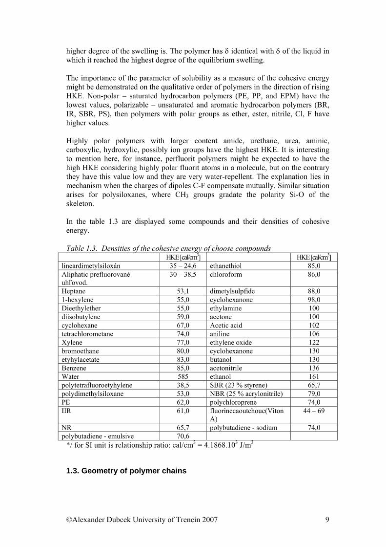
higher degree of the swelling is. The polymer has δ identical with δ of the liquid in which it reached the highest degree of the equilibrium swelling. The importance of the parameter of solubility as a measure of the cohesive energy might be demonstrated on the qualitative order of polymers in the direction of rising HKE. Non-polar – saturated hydrocarbon polymers (PE, PP, and EPM) have the lowest values, polarizable – unsaturated and aromatic hydrocarbon polymers (BR, IR, SBR, PS), then polymers with polar groups as ether, ester, nitrile, Cl, F have higher values. Highly polar polymers with larger content amide, urethane, urea, aminic, carboxylic, hydroxylic, possibly ion groups have the highest HKE. It is interesting to mention here, for instance, perfluorit polymers might be expected to have the high HKE considering highly polar fluorit atoms in a molecule, but on the contrary they have this value low and they are very water-repellent. The explanation lies in mechanism when the charges of dipoles C-F compensate mutually. Similar situation arises for polysiloxanes, where CH3 groups gradate the polarity Si-O of the skeleton. In the table 1.3 are displayed some compounds and their densities of cohesive energy. Table 1.3. Densities of the cohesive energy of choose compounds

HKE [cal/cm3] HKE [cal/cm3] lineardimetylsiloxán 35 – 24,6 ethanethiol 85,0 Aliphatic prefluorované uhľovod.

30 – 38,5 chloroform 86,0

Heptane 53,1 dimetylsulpfide 88,0 1-hexylene 55,0 cyclohexanone 98,0 Dieethylether 55,0 ethylamine 100 diisobutylene 59,0 acetone 100 cyclohexane 67,0 Acetic acid 102 tetrachlorometane 74,0 aniline 106 Xylene 77,0 ethylene oxide 122 bromoethane 80,0 cyclohexanone 130 etyhylacetate 83,0 butanol 130 Benzene 85,0 acetonitrile 136 Water 585 ethanol 161 polytetrafluoroetyhylene 38,5 SBR (23 % styrene) 65,7 polydimethylsiloxane 53,0 NBR (25 % acrylonitrile) 79,0 PE 62,0 polychloroprene 74,0 IIR 61,0 fluorinecaoutchouc(Viton

A) 44 – 69

NR 65,7 polybutadiene - sodium 74,0 polybutadiene - emulsive 70,6

*/ for SI unit is relationship ratio: cal/cm3 = 4.1868.103 J/m3

1.3. Geometry of polymer chains


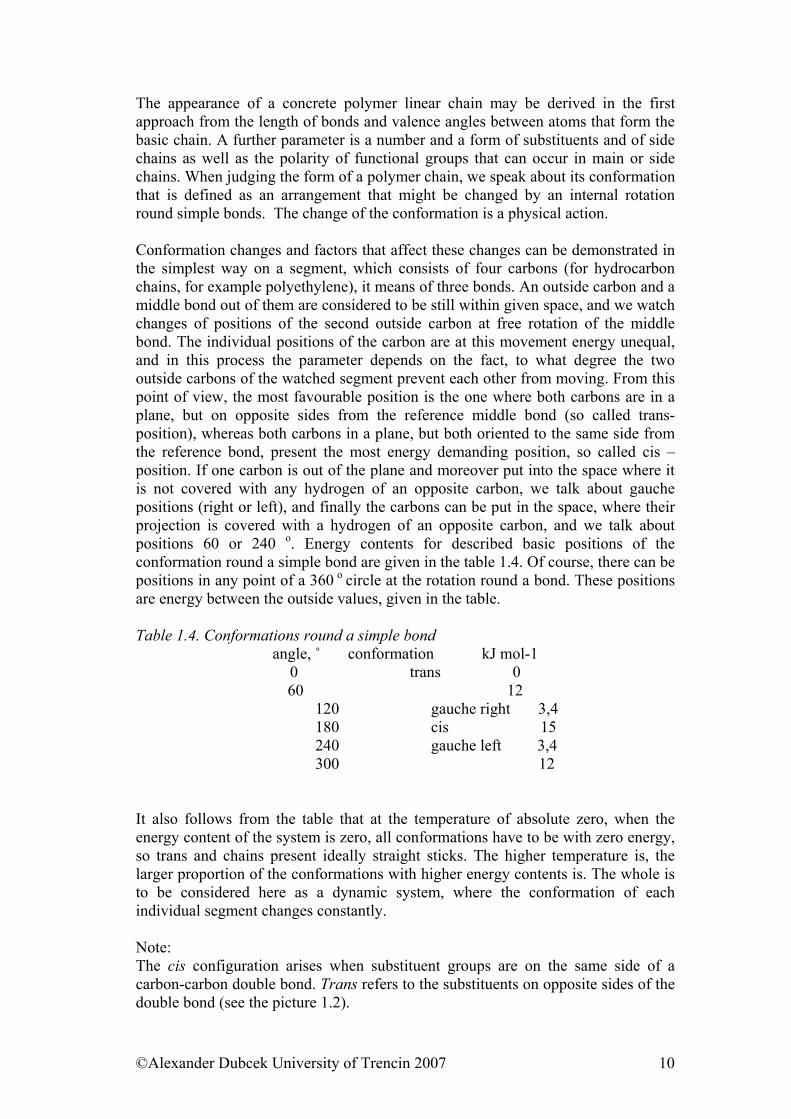
The appearance of a concrete polymer linear chain may be derived in the first approach from the length of bonds and valence angles between atoms that form the basic chain. A further parameter is a number and a form of substituents and of side chains as well as the polarity of functional groups that can occur in main or side chains. When judging the form of a polymer chain, we speak about its conformation that is defined as an arrangement that might be changed by an internal rotation round simple bonds. The change of the conformation is a physical action. Conformation changes and factors that affect these changes can be demonstrated in the simplest way on a segment, which consists of four carbons (for hydrocarbon chains, for example polyethylene), it means of three bonds. An outside carbon and a middle bond out of them are considered to be still within given space, and we watch changes of positions of the second outside carbon at free rotation of the middle bond. The individual positions of the carbon are at this movement energy unequal, and in this process the parameter depends on the fact, to what degree the two outside carbons of the watched segment prevent each other from moving. From this point of view, the most favourable position is the one where both carbons are in a plane, but on opposite sides from the reference middle bond (so called trans-position), whereas both carbons in a plane, but both oriented to the same side from the reference bond, present the most energy demanding position, so called cis – position. If one carbon is out of the plane and moreover put into the space where it is not covered with any hydrogen of an opposite carbon, we talk about gauche positions (right or left), and finally the carbons can be put in the space, where their projection is covered with a hydrogen of an opposite carbon, and we talk about positions 60 or 240 o. Energy contents for described basic positions of the conformation round a simple bond are given in the table 1.4. Of course, there can be positions in any point of a 360 o circle at the rotation round a bond. These positions are energy between the outside values, given in the table. Table 1.4. Conformations round a simple bond

angle, ˚ conformation kJ mol-1 0 trans 0 60 12

120 gauche right 3,4 180 cis 15 240 gauche left 3,4 300 12

It also follows from the table that at the temperature of absolute zero, when the energy content of the system is zero, all conformations have to be with zero energy, so trans and chains present ideally straight sticks. The higher temperature is, the larger proportion of the conformations with higher energy contents is. The whole is to be considered here as a dynamic system, where the conformation of each individual segment changes constantly. Note: The cis configuration arises when substituent groups are on the same side of a carbon-carbon double bond. Trans refers to the substituents on opposite sides of the double bond (see the picture 1.2).


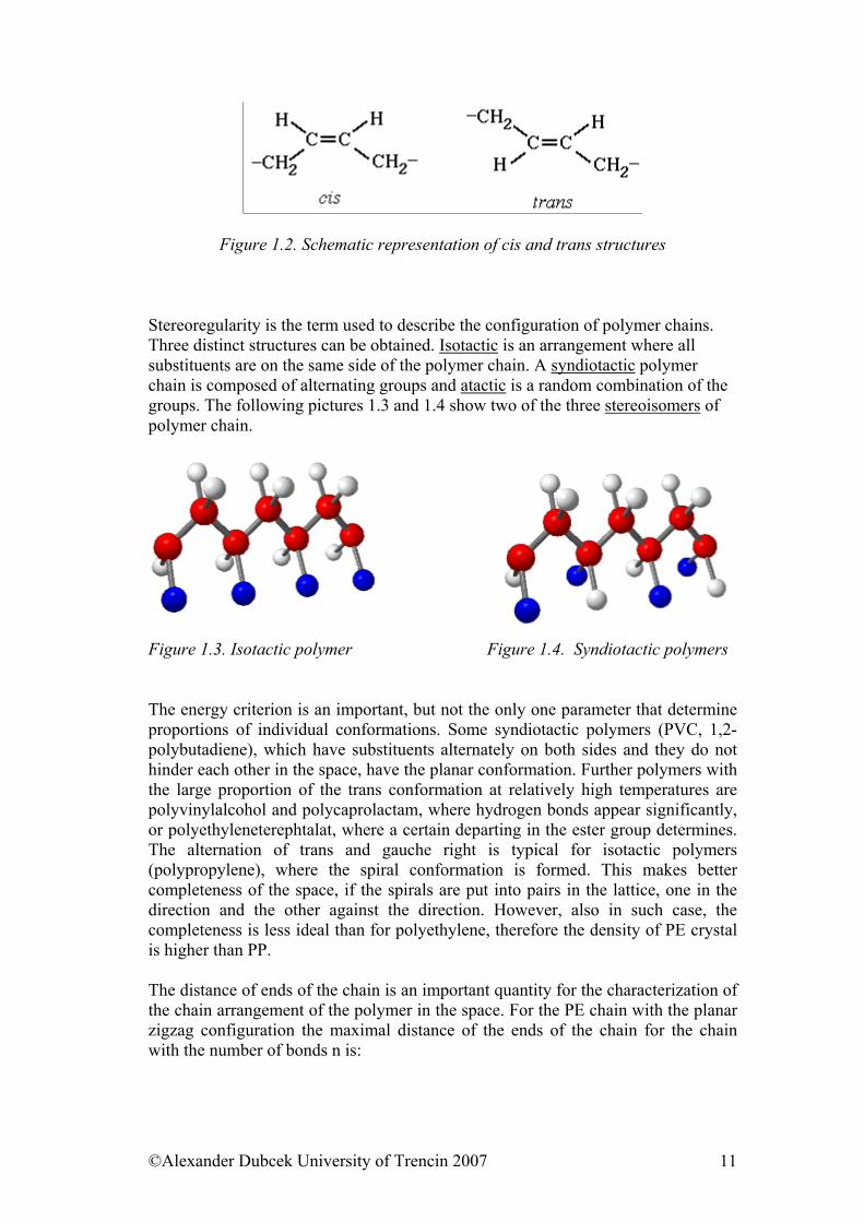
Figure 1.2. Schematic representation of cis and trans structures

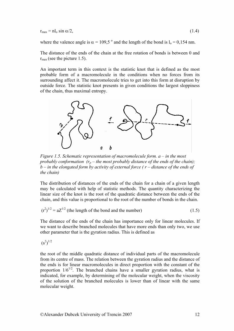
Stereoregularity is the term used to describe the configuration of polymer chains. Three distinct structures can be obtained. Isotactic is an arrangement where all substituents are on the same side of the polymer chain. A syndiotactic polymer chain is composed of alternating groups and atactic is a random combination of the groups. The following pictures 1.3 and 1.4 show two of the three stereoisomers of polymer chain.

Figure 1.3. Isotactic polymer Figure 1.4. Syndiotactic polymers

The energy criterion is an important, but not the only one parameter that determine proportions of individual conformations. Some syndiotactic polymers (PVC, 1,2-polybutadiene), which have substituents alternately on both sides and they do not hinder each other in the space, have the planar conformation. Further polymers with the large proportion of the trans conformation at relatively high temperatures are polyvinylalcohol and polycaprolactam, where hydrogen bonds appear significantly, or polyethyleneterephtalat, where a certain departing in the ester group determines. The alternation of trans and gauche right is typical for isotactic polymers (polypropylene), where the spiral conformation is formed. This makes better completeness of the space, if the spirals are put into pairs in the lattice, one in the direction and the other against the direction. However, also in such case, the completeness is less ideal than for polyethylene, therefore the density of PE crystal is higher than PP. The distance of ends of the chain is an important quantity for the characterization of the chain arrangement of the polymer in the space. For the PE chain with the planar zigzag configuration the maximal distance of the ends of the chain for the chain with the number of bonds n is:


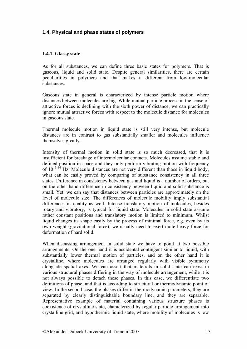
rmax = nlo sin α/2, (1.4) where the valence angle is α = 109,5 o and the length of the bond is lo = 0,154 nm. The distance of the ends of the chain at the free rotation of bonds is between 0 and rmax (see the picture 1.5). An important term in this context is the statistic knot that is defined as the most probable form of a macromolecule in the conditions when no forces from its surrounding affect it. The macromolecule tries to get into this form at disruption by outside force. The statistic knot presents in given conditions the largest sloppiness of the chain, thus maximal entropy.

Figure 1.5. Schematic representation of macromolecule form. a – in the most probably conformation (rp – the most probably distance of the ends of the chain); b – in the elongated form by activity of external force ( r – distance of the ends of the chain) The distribution of distances of the ends of the chain for a chain of a given length may be calculated with help of statistic methods. The quantity characterizing the linear size of the knot is the root of the quadratic distance between the ends of the chain, and this value is proportional to the root of the number of bonds in the chain. (r2)1/2 = aZ1/2 (the length of the bond and the number) (1.5) The distance of the ends of the chain has importance only for linear molecules. If we want to describe branched molecules that have more ends than only two, we use other parameter that is the gyration radius. This is defined as (s2)1/2

the root of the middle quadratic distance of individual parts of the macromolecule from its centre of mass. The relation between the gyration radius and the distance of the ends is for linear macromolecules in direct proportion with the constant of the proportion 1/61/2. The branched chains have a smaller gyration radius, what is indicated, for example, by determining of the molecular weight, when the viscosity of the solution of the branched molecules is lower than of linear with the same molecular weight.


1.4. Physical and phase states of polymers

1.4.1. Glassy state As for all substances, we can define three basic states for polymers. That is gaseous, liquid and solid state. Despite general similarities, there are certain peculiarities in polymers and that makes it different from low-molecular substances. Gaseous state in general is characterized by intense particle motion where distances between molecules are big. While mutual particle process in the sense of attractive forces is declining with the sixth power of distance, we can practically ignore mutual attractive forces with respect to the molecule distance for molecules in gaseous state. Thermal molecule motion in liquid state is still very intense, but molecule distances are in contrast to gas substantially smaller and molecules influence themselves greatly. Intensity of thermal motion in solid state is so much decreased, that it is insufficient for breakage of intermolecular contacts. Molecules assume stable and defined position in space and they only perform vibrating motion with frequency of 1013-14 Hz. Molecule distances are not very different than those in liquid body, what can be easily proved by comparing of substance consistency in all three states. Difference in consistency between gas and liquid is a number of orders, but on the other hand difference in consistency between liquid and solid substance is small. Yet, we can say that distances between particles are approximately on the level of molecule size. The differences of molecule mobility imply substantial differences in quality as well. Intense translatory motion of molecules, besides rotary and vibratory, is typical for liquid state. Molecules in solid state assume rather constant positions and translatory motion is limited to minimum. Whilst liquid changes its shape easily by the process of minimal force, e.g. even by its own weight (gravitational force), we usually need to exert quite heavy force for deformation of hard solid. When discussing arrangement in solid state we have to point at two possible arrangements. On the one hand it is accidental contingent similar to liquid, with substantially lower thermal motion of particles, and on the other hand it is crystalline, where molecules are arranged regularly with visible symmetry alongside spatial axes. We can assert that materials in solid state can exist in various structural phases differing in the way of molecule arrangement, while it is not always possible to detach these phases. In this case, we differentiate two definitions of phase, and that is according to structural or thermodynamic point of view. In the second case, the phases differ in thermodynamic parameters, they are separated by clearly distinguishable boundary line, and they are separable. Representative example of material containing various structure phases is coexistence of crystalline state, characterized by regular particle arrangement into crystalline grid, and hypothermic liquid state, where mobility of molecules is low


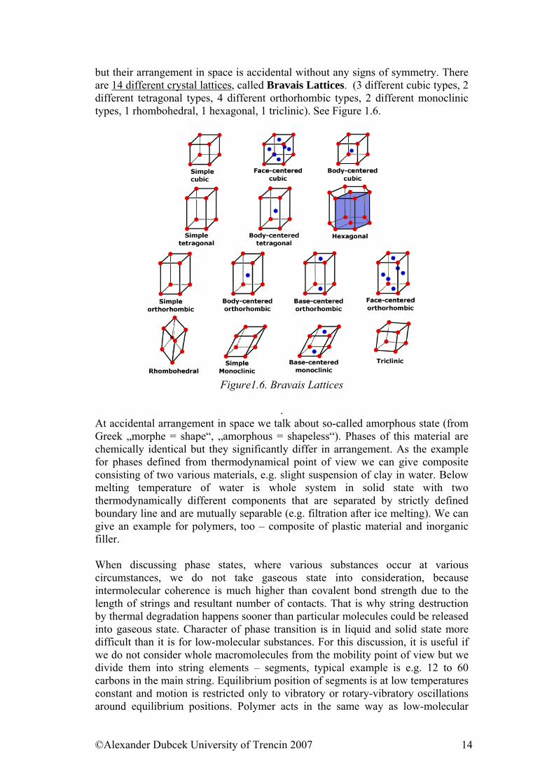
but their arrangement in space is accidental without any signs of symmetry. There are 14 different crystal lattices, called Bravais Lattices. (3 different cubic types, 2 different tetragonal types, 4 different orthorhombic types, 2 different monoclinic types, 1 rhombohedral, 1 hexagonal, 1 triclinic). See Figure 1.6.

Figure1.6. Bravais Lattices

.

At accidental arrangement in space we talk about so-called amorphous state (from Greek „morphe = shape“, „amorphous = shapeless“). Phases of this material are chemically identical but they significantly differ in arrangement. As the example for phases defined from thermodynamical point of view we can give composite consisting of two various materials, e.g. slight suspension of clay in water. Below melting temperature of water is whole system in solid state with two thermodynamically different components that are separated by strictly defined boundary line and are mutually separable (e.g. filtration after ice melting). We can give an example for polymers, too – composite of plastic material and inorganic filler. When discussing phase states, where various substances occur at various circumstances, we do not take gaseous state into consideration, because intermolecular coherence is much higher than covalent bond strength due to the length of strings and resultant number of contacts. That is why string destruction by thermal degradation happens sooner than particular molecules could be released into gaseous state. Character of phase transition is in liquid and solid state more difficult than it is for low-molecular substances. For this discussion, it is useful if we do not consider whole macromolecules from the mobility point of view but we divide them into string elements – segments, typical example is e.g. 12 to 60 carbons in the main string. Equilibrium position of segments is at low temperatures constant and motion is restricted only to vibratory or rotary-vibratory oscillations around equilibrium positions. Polymer acts in the same way as low-molecular


substance in solid state. At deformation application the whole system is following Hook’s law, Young’s modulus of elasticity is high and material is fragile. While behaviour of polymer is similar to glass qualities, we call it glassy state. Glassy state is observed at low temperatures up to so-called temperature of glassy transition. In the sphere of temperature of glassy transition Tg occurs qualitative change of segment motion that changes to rotary in the sphere above Tg. The string can acquire high number of various conformational shapes; material has lower modulus of elasticity and behaves as highly elastic solid.

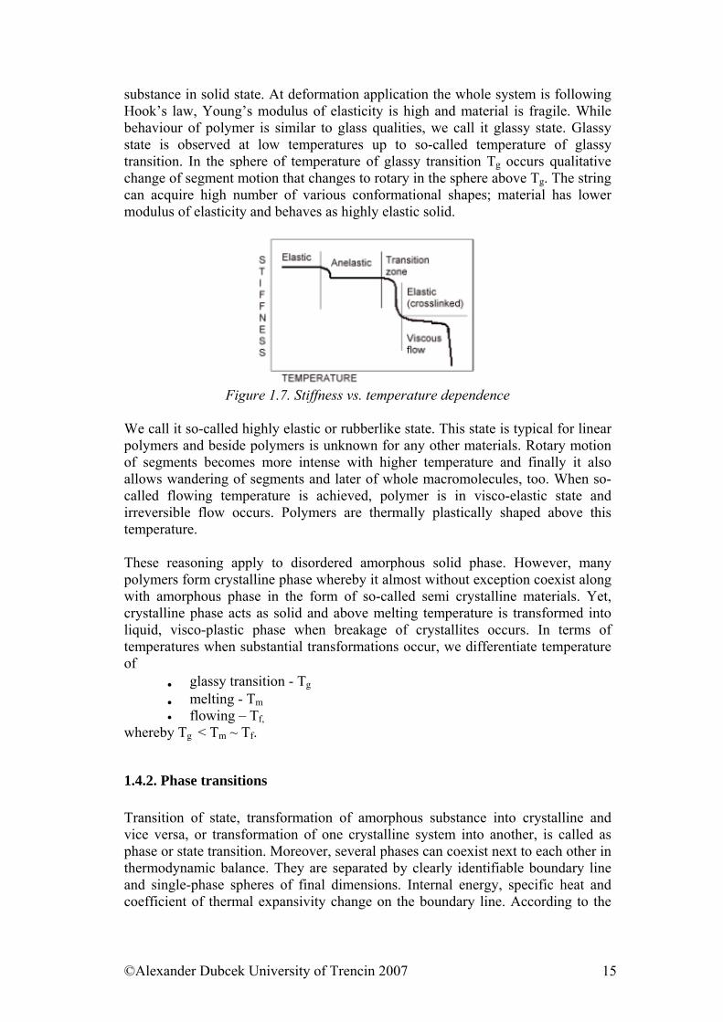
Figure 1.7. Stiffness vs. temperature dependence

We call it so-called highly elastic or rubberlike state. This state is typical for linear polymers and beside polymers is unknown for any other materials. Rotary motion of segments becomes more intense with higher temperature and finally it also allows wandering of segments and later of whole macromolecules, too. When so-called flowing temperature is achieved, polymer is in visco-elastic state and irreversible flow occurs. Polymers are thermally plastically shaped above this temperature. These reasoning apply to disordered amorphous solid phase. However, many polymers form crystalline phase whereby it almost without exception coexist along with amorphous phase in the form of so-called semi crystalline materials. Yet, crystalline phase acts as solid and above melting temperature is transformed into liquid, visco-plastic phase when breakage of crystallites occurs. In terms of temperatures when substantial transformations occur, we differentiate temperature of

• glassy transition - Tg

• melting - Tm • flowing – Tf,

whereby Tg < Tm ~ Tf.

1.4.2. Phase transitions Transition of state, transformation of amorphous substance into crystalline and vice versa, or transformation of one crystalline system into another, is called as phase or state transition. Moreover, several phases can coexist next to each other in thermodynamic balance. They are separated by clearly identifiable boundary line and single-phase spheres of final dimensions. Internal energy, specific heat and coefficient of thermal expansivity change on the boundary line. According to the


character of this transformation we talk of phase transitions of the first or second order. We determine phase transitions from dependencies of internal energy change and temperature growth. They can be experimentally simplest determined from thermal dependency of specific volume. Discontinuity can be observed at phase transition of the first order at both dependencies. Typical phase transition of the first order is melting or reversible process – solidification at melting/solidification point. At this point, e.g. at melting, we provide heat to the system and internal energy is increasing, temperature however does not change. After all the crystalline part is melted, the temperature starts to rise again (but it is temperature of liquid, now). We can also observe similar phenomenon when watching transformation of specific volume with temperature, where substantial change of this parameter without change of temperature occurs at melting point.

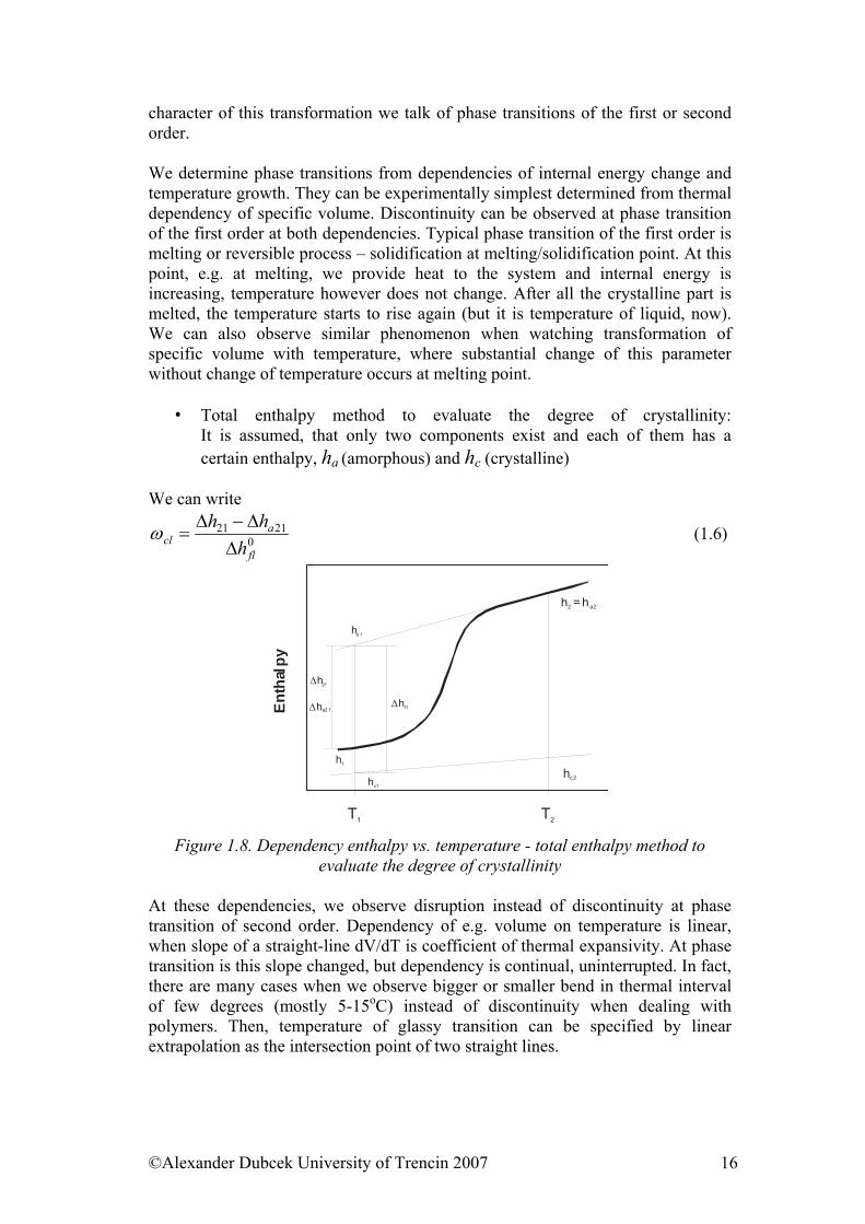
• Total enthalpy method to evaluate the degree of crystallinity: It is assumed, that only two components exist and each of them has a certain enthalpy, ha (amorphous) and hc (crystalline)

We can write

02121

fl

acl h

hh∆

∆−∆=ω (1.6)

T1 T2

h = h2 a2

hc2

h1

∆h21

∆ha2 1Enth

alpy

∆hf1

ha 1

hc1

Figure 1.8. Dependency enthalpy vs. temperature - total enthalpy method to

evaluate the degree of crystallinity

At these dependencies, we observe disruption instead of discontinuity at phase transition of second order. Dependency of e.g. volume on temperature is linear, when slope of a straight-line dV/dT is coefficient of thermal expansivity. At phase transition is this slope changed, but dependency is continual, uninterrupted. In fact, there are many cases when we observe bigger or smaller bend in thermal interval of few degrees (mostly 5-15oC) instead of discontinuity when dealing with polymers. Then, temperature of glassy transition can be specified by linear extrapolation as the intersection point of two straight lines.


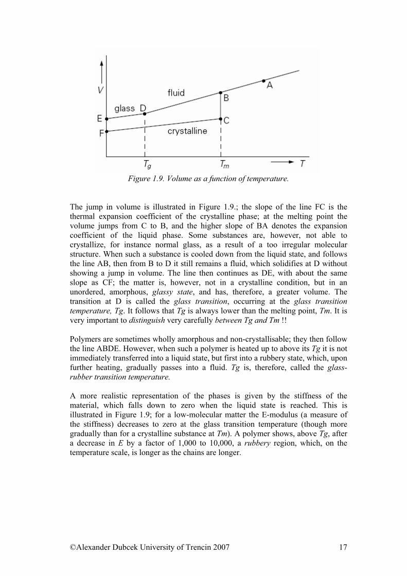
Figure 1.9. Volume as a function of temperature.

The jump in volume is illustrated in Figure 1.9.; the slope of the line FC is the thermal expansion coefficient of the crystalline phase; at the melting point the volume jumps from C to B, and the higher slope of BA denotes the expansion coefficient of the liquid phase. Some substances are, however, not able to crystallize, for instance normal glass, as a result of a too irregular molecular structure. When such a substance is cooled down from the liquid state, and follows the line AB, then from B to D it still remains a fluid, which solidifies at D without showing a jump in volume. The line then continues as DE, with about the same slope as CF; the matter is, however, not in a crystalline condition, but in an unordered, amorphous, glassy state, and has, therefore, a greater volume. The transition at D is called the glass transition, occurring at the glass transition temperature, Tg. It follows that Tg is always lower than the melting point, Tm. It is very important to distinguish very carefully between Tg and Tm !! Polymers are sometimes wholly amorphous and non-crystallisable; they then follow the line ABDE. However, when such a polymer is heated up to above its Tg it is not immediately transferred into a liquid state, but first into a rubbery state, which, upon further heating, gradually passes into a fluid. Tg is, therefore, called the glass-rubber transition temperature. A more realistic representation of the phases is given by the stiffness of the material, which falls down to zero when the liquid state is reached. This is illustrated in Figure 1.9; for a low-molecular matter the E-modulus (a measure of the stiffness) decreases to zero at the glass transition temperature (though more gradually than for a crystalline substance at Tm). A polymer shows, above Tg, after a decrease in E by a factor of 1,000 to 10,000, a rubbery region, which, on the temperature scale, is longer as the chains are longer.


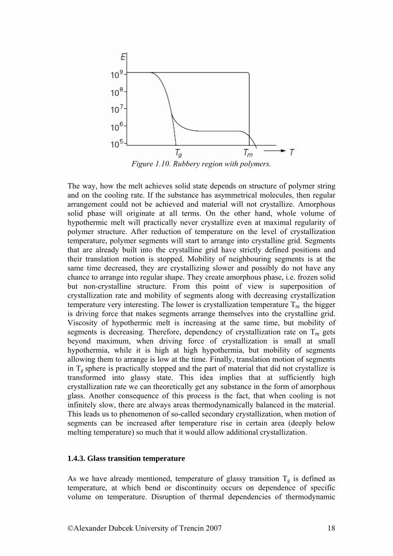
Figure 1.10. Rubbery region with polymers.

The way, how the melt achieves solid state depends on structure of polymer string and on the cooling rate. If the substance has asymmetrical molecules, then regular arrangement could not be achieved and material will not crystallize. Amorphous solid phase will originate at all terms. On the other hand, whole volume of hypothermic melt will practically never crystallize even at maximal regularity of polymer structure. After reduction of temperature on the level of crystallization temperature, polymer segments will start to arrange into crystalline grid. Segments that are already built into the crystalline grid have strictly defined positions and their translation motion is stopped. Mobility of neighbouring segments is at the same time decreased, they are crystallizing slower and possibly do not have any chance to arrange into regular shape. They create amorphous phase, i.e. frozen solid but non-crystalline structure. From this point of view is superposition of crystallization rate and mobility of segments along with decreasing crystallization temperature very interesting. The lower is crystallization temperature Tm the bigger is driving force that makes segments arrange themselves into the crystalline grid. Viscosity of hypothermic melt is increasing at the same time, but mobility of segments is decreasing. Therefore, dependency of crystallization rate on Tm gets beyond maximum, when driving force of crystallization is small at small hypothermia, while it is high at high hypothermia, but mobility of segments allowing them to arrange is low at the time. Finally, translation motion of segments in Tg sphere is practically stopped and the part of material that did not crystallize is transformed into glassy state. This idea implies that at sufficiently high crystallization rate we can theoretically get any substance in the form of amorphous glass. Another consequence of this process is the fact, that when cooling is not infinitely slow, there are always areas thermodynamically balanced in the material. This leads us to phenomenon of so-called secondary crystallization, when motion of segments can be increased after temperature rise in certain area (deeply below melting temperature) so much that it would allow additional crystallization.

1.4.3. Glass transition temperature As we have already mentioned, temperature of glassy transition Tg is defined as temperature, at which bend or discontinuity occurs on dependence of specific volume on temperature. Disruption of thermal dependencies of thermodynamic


functions, such as enthalpy and entropy, occurs in the same thermal sphere. First derivation of basic thermodynamic functions, thermal coefficient of volume dV/dT and thermal coefficient of enthalpy dH/dT = Cp (thermal capacity) are changed discontinuously. Thermal coefficients of transport qualities, such as viscosity, diffusion of gases and stress relaxation are changed discontinuously, too, whereby modulus of elasticity increases by few orders. Absorption of mechanical and electrical energy reaches maximum. There are several methods for the determination of glass transition temperature, in addition to the use of changes in quality in Tg sphere. Tg can be determined e.g. dilatometrically, by watching thermal expansivity. Other commonly used method is calorimetric method, mostly differential scanning calorimetry, DSC. Dynamical-mechanical analysis is another important method that is used for direct detection of certain motion releases at gradual temperature increase, whereby the most significant response is observed at motion release of main string segments that correspond with temperature Tg. Methods of Tg determination are related to important parameter, so-called free volume. We can explain the conception of free volume by following reasoning. Molecules in hard solid are not arranged totally tight, there are free vacancies between them. These relate with freezing or restriction of motion in real time in certain state. Thermal volume expansion occurs at temperature increase. Yet, single volume of molecule almost never changes with temperature. Practically, only the area between molecules is changing and mobility of molecules increases at the same time. According to Cohen and Turnbull theory, redistribution of size of vacancies in liquid occurs relentlessly, whereby molecule can skip only to the space with at least particular minimal volume. Skip frequency is determined not by energetic factors, but by probabilistic factors, where critical volume is very important quantity. Probability that certain molecule will skip to the other place is determined by probability that there is large enough vacancy in its vicinity. Thermal volume expansion is caused by the growth of free volume. Probability can be expressed by quantity f as the quotient of occupied and unoccupied space. Dependence of f on temperature is linear f = αf (T - T∞) (1.7) where T and T∞ is system temperature and reference temperature and αf is coefficient of thermal expansivity. On basis of these presumptions we can infer theorems for diffusion coefficient D D = D∞ exp (-1 / αf (T - T∞) (1.8) or other quantities, e.g. viscosity η η = η∞ exp (-1 / αf (T - T∞) (1.9) Alternative to probabilistic theories are energetic theories. Skip of liquid particle is according to them possible only when the particle has certain superfluous energy


that will allow it to overcome the energetic barrier. Thermal dependencies are two-parameter and have the form of Arrhenius equation D = D∞ e-Ea/RT (1.10) where Ea can be considered as activation energy or thermal coefficient of particular process. At the same time we have to realize that total energy of system depends on temperature, but energy of every particular element (or moving segment in the case of polymers) is not identical with other particles and it is neither constant. Particles (segments) collide with each other and they transfer energy. Accidentally, some particle can gain energy that would suffice to break energetic barrier created by neighbouring particles. Rearrangement – translation motion will happen in such case. At temperature T = 0 K, diffusion coefficient decreases to zero and viscosity gains infinite value. In 1921, Vogel, Fulcher and Tamman inferred important empiric equation during study of inorganic glass viscosity. It allows direct calculation of melt viscosity η for any temperature T, if constant B and viscosity η∞ was experimentally determined at reference temperature T∞

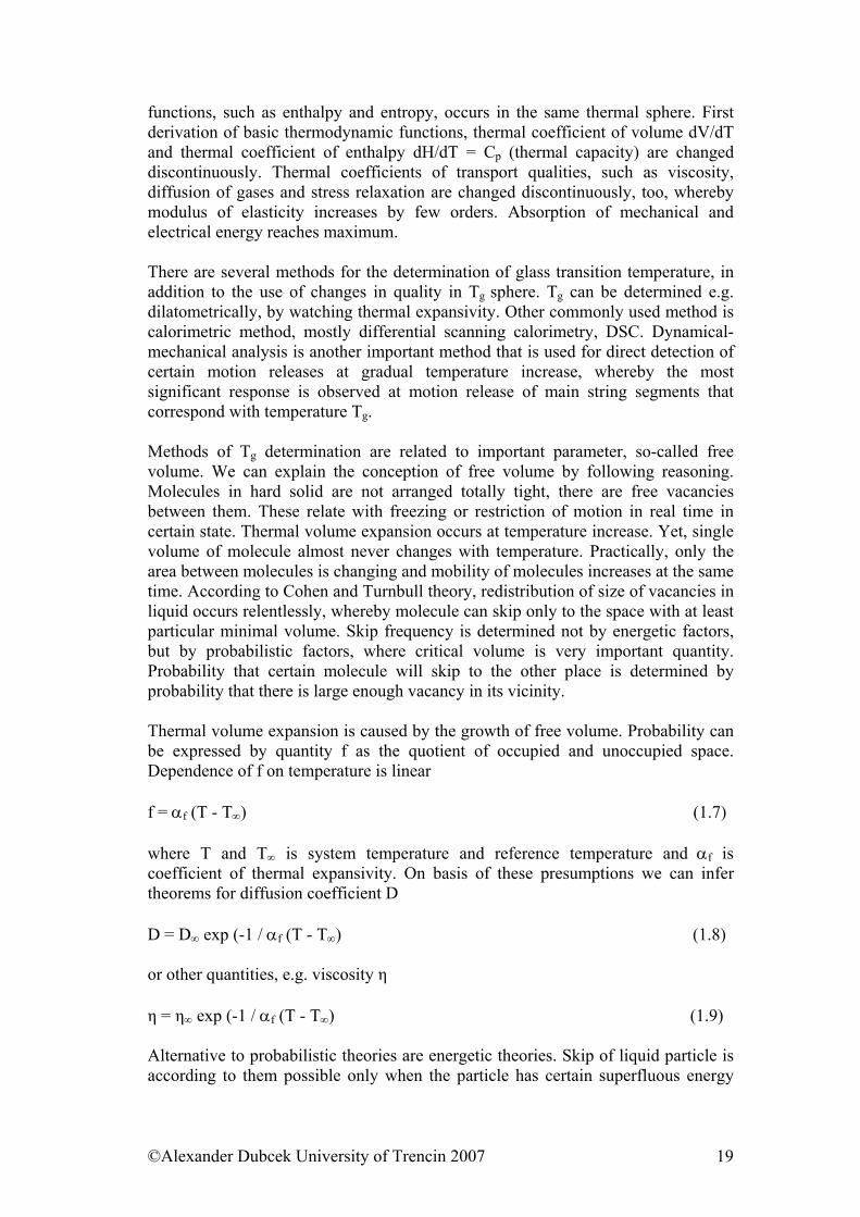
logη = logη∞ + B / (T - T∞) (1.11) In confrontation of theorems (1.7) and (1.11) we can see that αf = log e / B. (1.12) Williams - Landel, – Ferry in 1953 proposed another crucial semiempirical equation. They have chosen Tg for reference temperature and ηg is viscosity at Tg. This equation has form log η / ηg = -c1g (T - Tg) / c2g + T - Tg (1.13) and is so important that it is called WLF equation. WLF equation is a law for determining frequency temperature equivalence (which holds true for a given range). To have an approximate idea, it can be considered that, in low frequencies (from 10 to 105 Hz), an increase in frequency by a factor of 10 has the same effect on the behaviour of the rubber as a 7 to 8°C drop in temperature. For example, an elastomer with a glass transition temperature of -20°C at 10 Hz will have a glass transition temperature of about +10°C at 105 Hz.


100

200

400

800

1600

3200

-40 -30 -20 -10 0 10 20 30 40Temperature Co

Glass transition temperature (Tg)

Modulus

Rubberystate

Glassystate

Figure 1.11. Modulus vs. temperature dependency for 10 Hz

The above graph is plotted for a frequency of 10 Hz. Using the WLF equation, the graph can be calculated for other stress frequencies (see below).

100

200

400

800

1600

3200

-40 -30 -20 -10 0 10 20 30 40Temperature Co

Glass transition temperature (Tg)

Modulus

Rubberystate

Glassystate

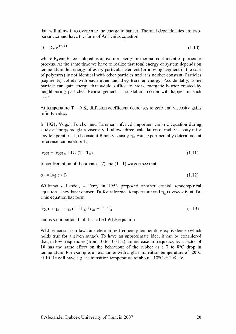
Figure 1.12. Modulus vs. temperature dependency for 105 Hz

For any given rubber, the glass transition temperature increases with the stress frequency, which moves the vitreous state towards higher temperatures.


line

of T

gGlassy zone

Rubbery zone

Frequencylog

-50 0 50 100 150

0

2

6

8

4

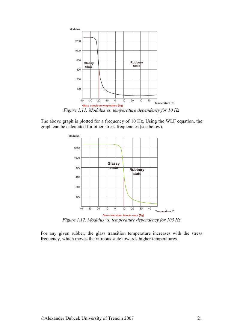
T in Co Figure 1.13. Frequency in log vs. temperature dependency

According to WLF equation, we can calculate viscosity η at temperature T on the basis of known viscosity ηg at temperature Tg, where c1g and c2g are empirical parameters. WLF equation can be inferred from Vogel’s equation in such a way that we substitute coordinates of reference point of ηg a Tg for basic parameters. After substitution c1g = B / Tg - T∞ (1.14) and c2g = Tg - T∞ (1.15) we get WLF equation. Constants c1g and c2g are in this case almost truly independent of temperature if we use Tg as reference temperature. Universal (average) values of the constants are c1g = 17.4 and c2g = 52 K. According to previous equations (1.14) and (1.15) we can express αf = 1/2.3 c1gc2g (1.16) and fg = 1/2.3c1g (1.17) When applying universal constants c1g and c2g we get universal values αf = 4.8 x 10-

4 K and fg = 0.025. At the same time we watch good agreement of universal αf with


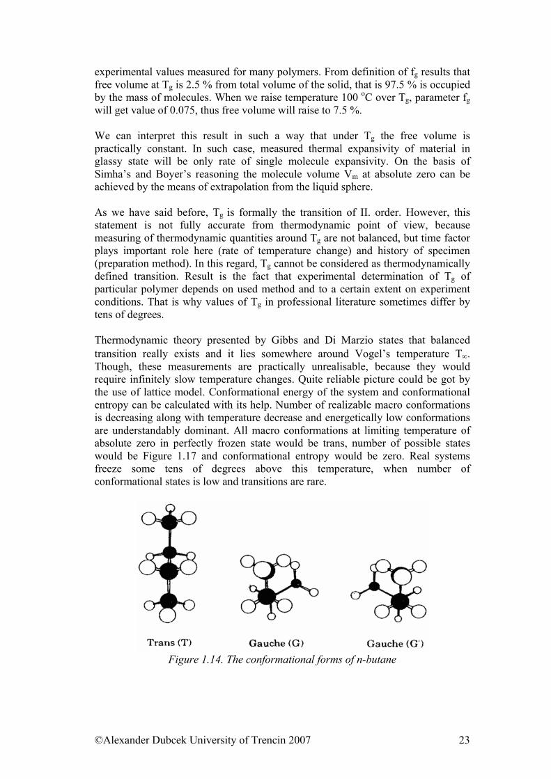
experimental values measured for many polymers. From definition of fg results that free volume at Tg is 2.5 % from total volume of the solid, that is 97.5 % is occupied by the mass of molecules. When we raise temperature 100 oC over Tg, parameter fg will get value of 0.075, thus free volume will raise to 7.5 %. We can interpret this result in such a way that under Tg the free volume is practically constant. In such case, measured thermal expansivity of material in glassy state will be only rate of single molecule expansivity. On the basis of Simha’s and Boyer’s reasoning the molecule volume Vm at absolute zero can be achieved by the means of extrapolation from the liquid sphere. As we have said before, Tg is formally the transition of II. order. However, this statement is not fully accurate from thermodynamic point of view, because measuring of thermodynamic quantities around Tg are not balanced, but time factor plays important role here (rate of temperature change) and history of specimen (preparation method). In this regard, Tg cannot be considered as thermodynamically defined transition. Result is the fact that experimental determination of Tg of particular polymer depends on used method and to a certain extent on experiment conditions. That is why values of Tg in professional literature sometimes differ by tens of degrees. Thermodynamic theory presented by Gibbs and Di Marzio states that balanced transition really exists and it lies somewhere around Vogel’s temperature T∞. Though, these measurements are practically unrealisable, because they would require infinitely slow temperature changes. Quite reliable picture could be got by the use of lattice model. Conformational energy of the system and conformational entropy can be calculated with its help. Number of realizable macro conformations is decreasing along with temperature decrease and energetically low conformations are understandably dominant. All macro conformations at limiting temperature of absolute zero in perfectly frozen state would be trans, number of possible states would be Figure 1.17 and conformational entropy would be zero. Real systems freeze some tens of degrees above this temperature, when number of conformational states is low and transitions are rare.

Figure 1.14. The conformational forms of n-butane


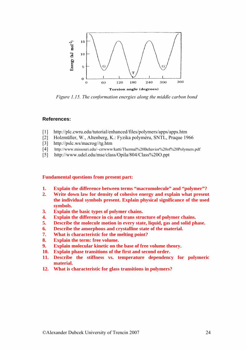
Figure 1.15. The conformation energies along the middle carbon bond

References: [1] http://plc.cwru.edu/tutorial/enhanced/files/polymers/apps/apps.htm [2] Holzmüller, W., Altenberg, K.: Fyzika polyméru, SNTL, Praque 1966 [3] http://pslc.ws/macrog//tg.htm [4] http://www.missouri.edu/~crrwww/katti/Thermal%20Behavior%20of%20Polymers.pdf [5] http://www.udel.edu/mse/class/Opila/804/Class%20O.ppt

Fundamental questions from present part: 1. Explain the difference between terms “macromolecule” and “polymer”? 2. Write down law for density of cohesive energy and explain what present

the individual symbols present. Explain physical significance of the used symbols.

3. Explain the basic types of polymer chains. 4. Explain the difference in cis and trans structure of polymer chains. 5. Describe the molecule motion in every state, liquid, gas and solid phase. 6. Describe the amorphous and crystalline state of the material. 7. What is characteristic for the melting point? 8. Explain the term: free volume. 9. Explain molecular kinetic on the base of free volume theory. 10. Explain phase transitions of the first and second order. 11. Describe the stiffness vs. temperature dependency for polymeric

material. 12. What is characteristic for glass transitions in polymers?


CHAPTER 2 Mechanical properties of solid state polymers

Objectives to achieve In this part we are going to deal with a description of deformation of solid elastic materials as well as to set up phenomenological values describing mechanical properties of these substances. We are going to learn about thermodynamic and microstructural aspects of the process of elastic deformation. Later on these concepts and knowledge will be generalized on polymers and rubber.

2.1. Description of deformation of solid elastic materials

Deformation of solid elastic materials can be found in the change of relative positions of their atoms and molecules as a result of external forces. For this reason, appropriate description of this phenomenon should issue from the calculation of displacement of individual atoms compared to state without the effect of external forces. On the base of practical reasoning, however, we imagine the substance as a continuum, we describe particular deformations with the help of appropriately applied elastic constants, modulus of elasticity and until then we try to put these constants into continuity with atomic structure of the substance and with bonding between individual atoms. Concerning “direction” properties of bonds we can expect that crystals are in general deformed anisotropically and for that reason their deformation properties will be described by tensors (strain tensor, stress tensor, and so on).

However we are going to focus our attention on a description of deformation of isotropic substances because - in majority of cases regarding rubber and polymers - we are able to manage with this simplified description.

Let’s analyze deformation curve well known from the study of mechanical properties of metallic materials. To consider deformability of solid elastic materials we use the term stress (σ ), that is the force affecting the unit surface of solid elastic materials and strain (ε ) modified by elongation proportion ( ) and primary length (l

l∆0). The most commonly observed stress - strain dependence has a shape of

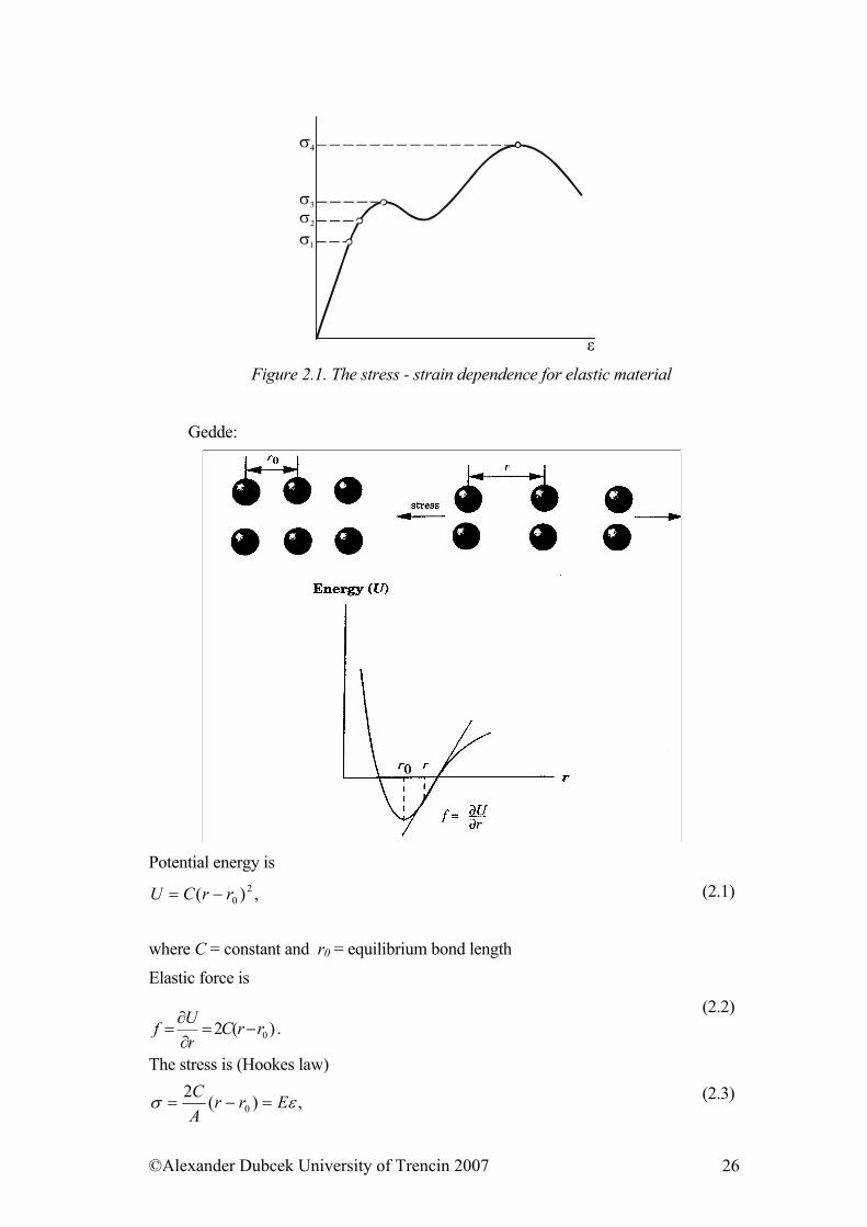
curve shown in figure 2.1.


σ1

σ4

σ3

σ2

ε Figure 2.1. The stress - strain dependence for elastic material

Gedde:

Potential energy is

(2.1) ,)( 20rrCU −=

where C = constant and r0 = equilibrium bond length

Elastic force is

(2.2) .)(2 0rrC

rU

−=∂∂

=f

The stress is (Hookes law)

(2.3) ,)(20 εσ Err

AC

=−=


where A = cross-sectional area, ε = strain

This dependence has few characteristic areas. First area is one of linear dependence where strain is directly proportional to stress. The prolongation itself is trivially small (<0,01%). When the action of external force is brought to an end, material returns to its previous state. The borderline of this area is limit of proportionality ( ). Within the influence of higher stress than the limit of elasticity, the material still deforms elastically, even though not linearly.

1σ

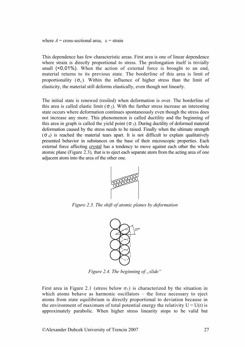
The initial state is renewed (resiled) when deformation is over. The borderline of this area is called elastic limit (σ 2). With the further stress increase an interesting state occurs where deformation continues spontaneously even though the stress does not increase any more. This phenomenon is called ductility and the beginning of this area in graph is called the yield point (σ 3). During ductility of deformed material deformation caused by the stress needs to be raised. Finally when the ultimate strength (σ 4) is reached the material tears apart. It is not difficult to explain qualitatively presented behavior in substances on the base of their microscopic properties. Each external force affecting crystal has a tendency to move against each other the whole atomic plane (Figure 2.3), that is to eject each separate atom from the acting area of one adjacent atom into the area of the other one.

Figure 2.3. The shift of atomic planes by deformation

27

Figure 2.4. The beginning of „slide“

First area in Figure 2.1 (stress below σ1) is characterized by the situation in which atoms behave as harmonic oscillators – the force necessary to eject atoms from state equilibrium is directly proportional to deviation because in the environment of maximum of total potential energy the relativity U = U(r) is approximately parabolic. When higher stress linearity stops to be valid but


deformation is still elastic up to the area equivalent to the situation shown in Figure 2.3. Corresponding angle is approximately 27°. Then it is not necessary to increase the stress deformation itself happens by „slide" of individual planes. That is how the sphere of ductility originates. Related stress (σ 3) can be considered the measured ultimate strength of material. On the base of well known results we can try to obtain quantitative estimation of ductility stress. This stress is approximately determined by the force, needed for releasing, all atoms of unit plane from bonds (Np) by their displacement (d). Pursuit of this force (σ 3d) has to be equal to the bond of energy Np of atoms (Np Ev), so for ductility stress we will reach a simple relation of

dEN

=σ vp3 (2.4)

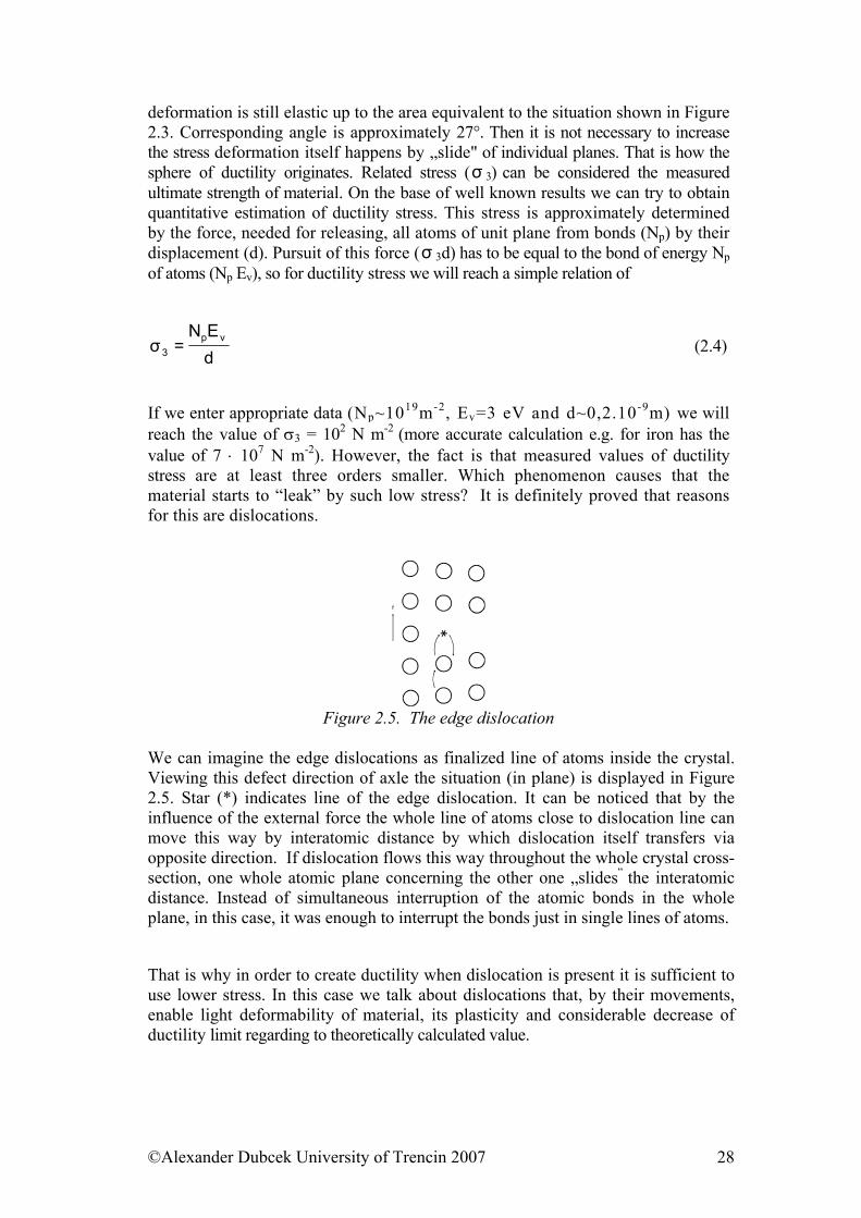
If we enter appropriate data (Np~1019m-2, Ev=3 eV and d~0,2.10-9m) we will reach the value of σ3 = 102 N m-2 (more accurate calculation e.g. for iron has the value of 7 ⋅ 107 N m-2). However, the fact is that measured values of ductility stress are at least three orders smaller. Which phenomenon causes that the material starts to “leak” by such low stress? It is definitely proved that reasons for this are dislocations.

f

Figure 2.5. The edge dislocation

We can imagine the edge dislocations as finalized line of atoms inside the crystal. Viewing this defect direction of axle the situation (in plane) is displayed in Figure 2.5. Star (*) indicates line of the edge dislocation. It can be noticed that by the influence of the external force the whole line of atoms close to dislocation line can move this way by interatomic distance by which dislocation itself transfers via opposite direction. If dislocation flows this way throughout the whole crystal cross-section, one whole atomic plane concerning the other one „slides“ the interatomic distance. Instead of simultaneous interruption of the atomic bonds in the whole plane, in this case, it was enough to interrupt the bonds just in single lines of atoms.

That is why in order to create ductility when dislocation is present it is sufficient to use lower stress. In this case we talk about dislocations that, by their movements, enable light deformability of material, its plasticity and considerable decrease of ductility limit regarding to theoretically calculated value.


If the listed reflections are true then it must be possible to reach the increase of metal strength by preparation without dislocation. These crystals can be produced only through high technology and only in very small contents.

Crystals produced in this manner are truly reaching theoretically calculated strength (iron wire with diameter of 1 mm can sustain the weight up to 1 000 kg).

Real crystals always contain dislocations and by their straining more dislocations are generated (by Frank—Read mechanism).

But when their concentration reaches the value of ~102m-3, they start to interfere when moving. This way the possibility of light strain decreases. The crystal is strengthened as a consequence of redundancy of dislocations. There through the area between σ 3 and σ 4 in figure 2.1 can be naturally explained. The knowledge - that through the restrain of dislocation movement it is possible to strengthen the crystal - is practically used. In polycrystalline structure the dislocation mobility is obviously smaller than in crystalline structure and for this reason these substances should have higher strength. It has been really approved. But in practice the most commonly used possibility is a different obstruction of dislocation movement - deliberate application of small amounts of suitable elements into crystals. These atoms obstruct dislocations movement very effectively and that is why for example iron with little amounts of carbon, chrome, magnesium and wolfram have vastly higher strength.

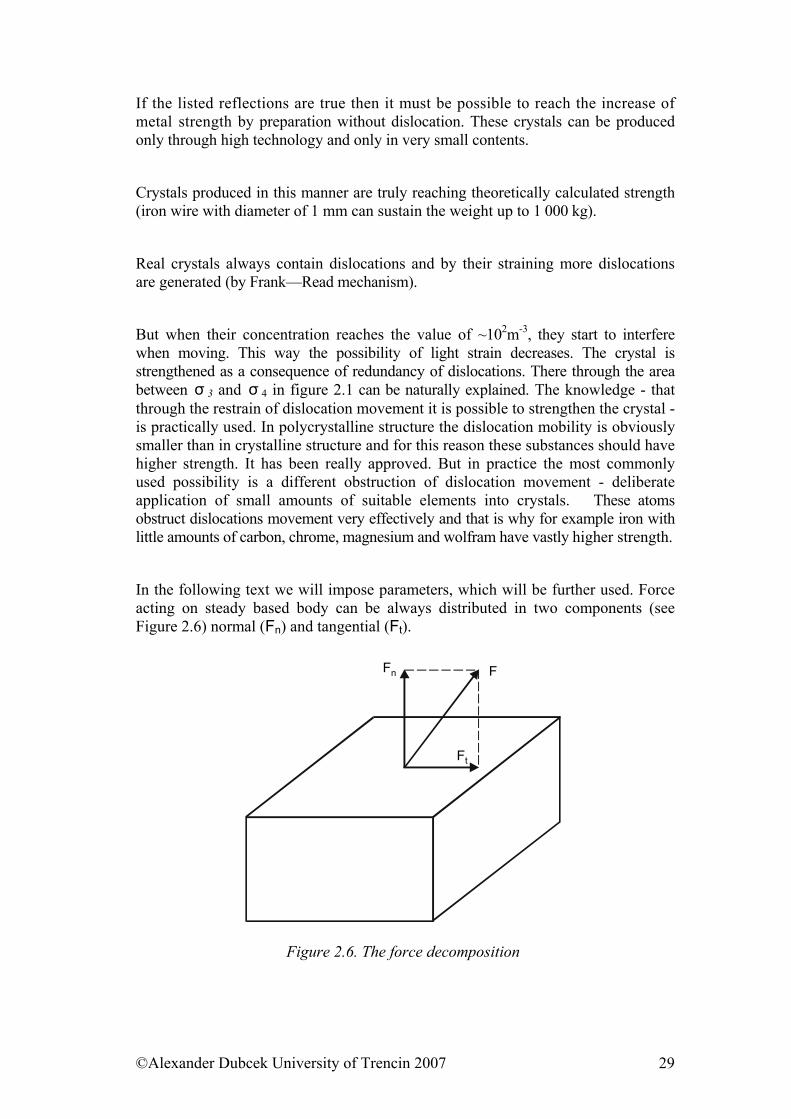
In the following text we will impose parameters, which will be further used. Force acting on steady based body can be always distributed in two components (see Figure 2.6) normal (Fn) and tangential (Ft).

Fn

Ft

F

Figure 2.6. The force decomposition


We define relevant strains by the following relations

SFσ n=⊥ , (2.5)

SF

=σ=T ttan . (2.6)

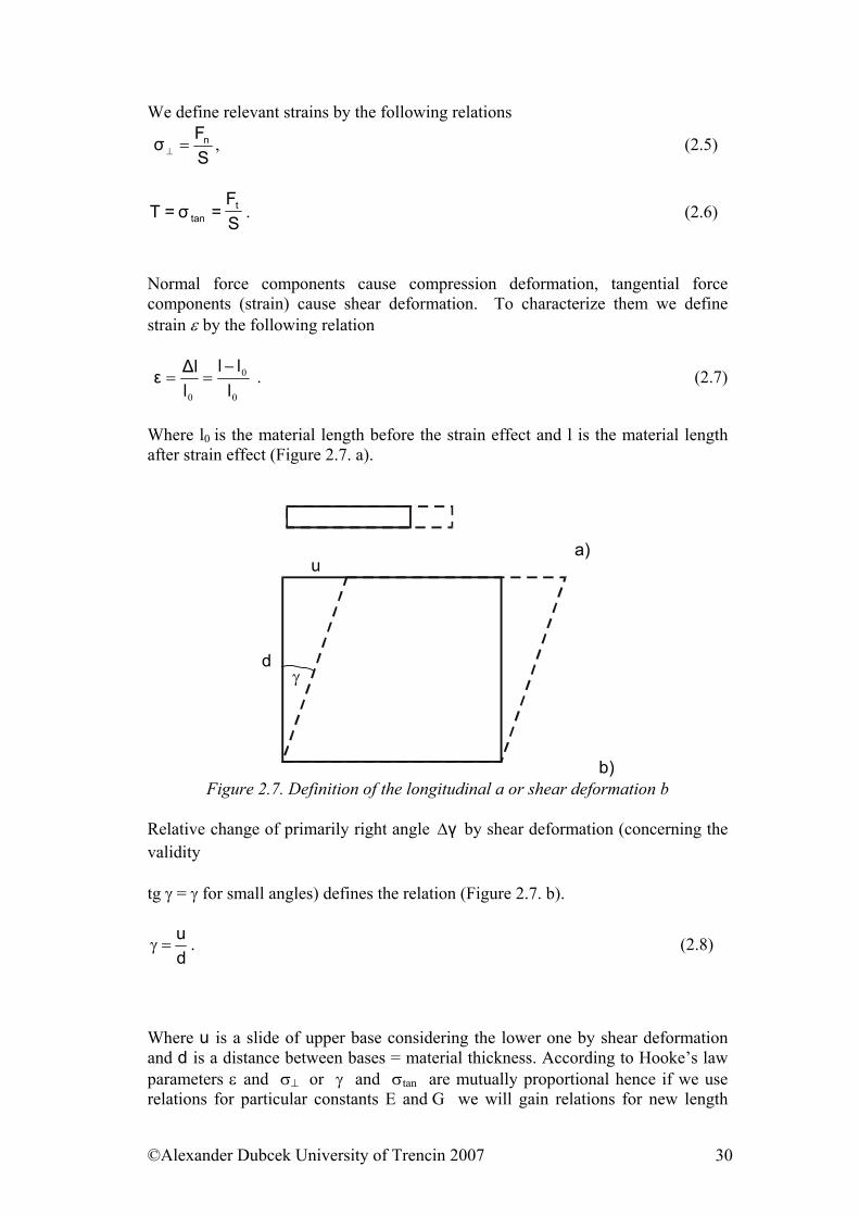
Normal force components cause compression deformation, tangential force components (strain) cause shear deformation. To characterize them we define strain ε by the following relation

0

0

0 lll

ll∆ε −

== . (2.7)

Where l0 is the material length before the strain effect and l is the material length after strain effect (Figure 2.7. a).

a) u

dγ

b) Figure 2.7. Definition of the longitudinal a or shear deformation b

Relative change of primarily right angle γ∆ by shear deformation (concerning the validity tg γ = γ for small angles) defines the relation (Figure 2.7. b).

du

=γ . (2.8)

Where u is a slide of upper base considering the lower one by shear deformation and d is a distance between bases = material thickness. According to Hooke’s law parameters ε and σ⊥ or γ and σtan are mutually proportional hence if we use relations for particular constants E and G we will gain relations for new length


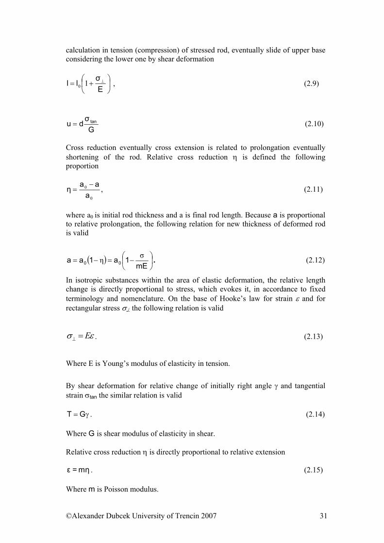
calculation in tension (compression) of stressed rod, eventually slide of upper base considering the lower one by shear deformation

⎟⎠

⎞⎜⎝

⎛ += ⊥

Eσll 10 , (2.9)

Gσdu tan= (2.10)

Cross reduction eventually cross extension is related to prolongation eventually shortening of the rod. Relative cross reduction η is defined the following proportion

0

0

aaa

η−

= , (2.11)

where a0 is initial rod thickness and a is final rod length. Because a is proportional to relative prolongation, the following relation for new thickness of deformed rod is valid

( ) ⎟⎠⎞

⎜⎝⎛ −=−=

mE1a1aa 00

ση . (2.12)

In isotropic substances within the area of elastic deformation, the relative length change is directly proportional to stress, which evokes it, in accordance to fixed terminology and nomenclature. On the base of Hooke’s law for strain ε and for rectangular stress σ⊥ the following relation is valid

εσ E=⊥ . (2.13)

Where E is Young’s modulus of elasticity in tension.

By shear deformation for relative change of initially right angle γ and tangential strain σtan the similar relation is valid

γ= GT . (2.14) Where G is shear modulus of elasticity in shear. Relative cross reduction η is directly proportional to relative extension

ηm=ε . (2.15) Where m is Poisson modulus.


Poisson’s number ν is inverted value of Poisson modulus so we use

m1

=ν . (2.16)

We usually choose E and ν as constants characterizing elastic properties of isotropic material. There is a mutual relation among three elastic constants E, G and m expressed as follows

( )1+m2Em

=G (2.17)

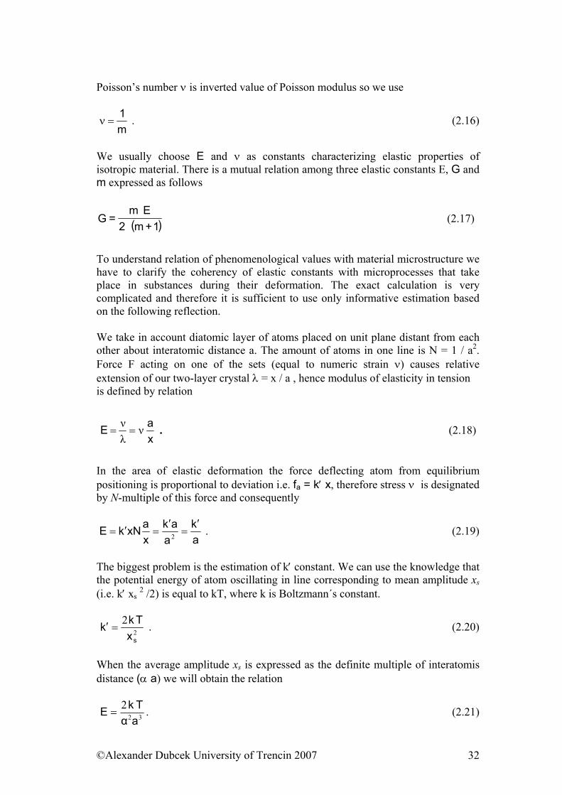
To understand relation of phenomenological values with material microstructure we have to clarify the coherency of elastic constants with microprocesses that take place in substances during their deformation. The exact calculation is very complicated and therefore it is sufficient to use only informative estimation based on the following reflection. We take in account diatomic layer of atoms placed on unit plane distant from each other about interatomic distance a. The amount of atoms in one line is N = 1 / a2. Force F acting on one of the sets (equal to numeric strain ν) causes relative extension of our two-layer crystal λ = x / a , hence modulus of elasticity in tension is defined by relation

xaE ν

λν

== . (2.18)

In the area of elastic deformation the force deflecting atom from equilibrium positioning is proportional to deviation i.e. fa = k′ x, therefore stress ν is designated by N-multiple of this force and consequently

ak

aak

xaxNkE

′=

′=′= 2 . (2.19)

The biggest problem is the estimation of k′ constant. We can use the knowledge that the potential energy of atom oscillating in line corresponding to mean amplitude xs (i.e. k′ xs 2 /2) is equal to kT, where k is Boltzmann´s constant.

2

2

sxTkk =′ . (2.20)

When the average amplitude xs is expressed as the definite multiple of interatomis distance (α a) we will obtain the relation

32

2aαTkE = . (2.21)


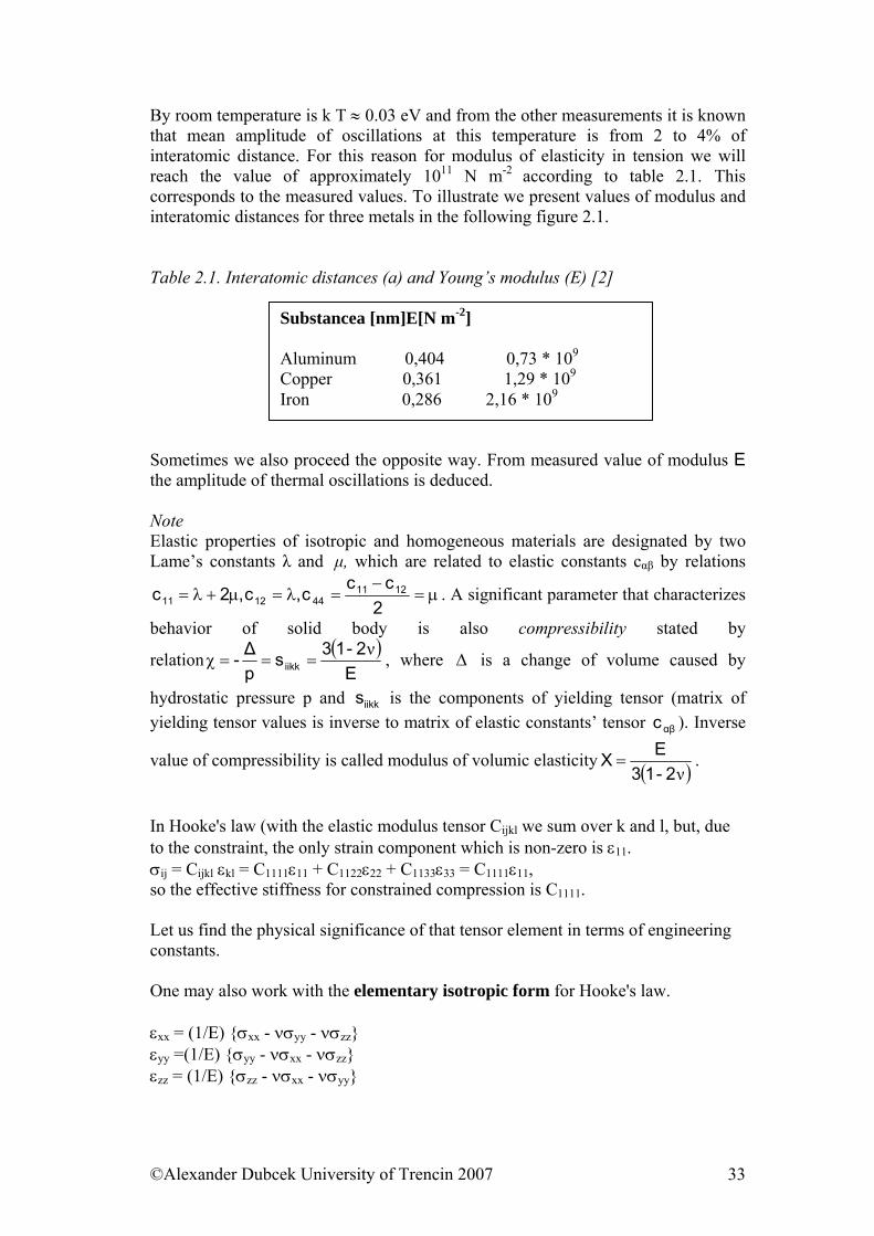
By room temperature is k T ≈ 0.03 eV and from the other measurements it is known that mean amplitude of oscillations at this temperature is from 2 to 4% of interatomic distance. For this reason for modulus of elasticity in tension we will reach the value of approximately 1011 N m-2 according to table 2.1. This corresponds to the measured values. To illustrate we present values of modulus and interatomic distances for three metals in the following figure 2.1. Table 2.1. Interatomic distances (a) and Young’s modulus (E) [2]

Substancea [nm]E[N m-2] Aluminum 0,404 0,73 * 109 Copper 0,361 1,29 * 109 Iron 0,286 2,16 * 109

Sometimes we also proceed the opposite way. From measured value of modulus E the amplitude of thermal oscillations is deduced. Note Elastic properties of isotropic and homogeneous materials are designated by two Lame’s constants λ and µ, which are related to elastic constants cαβ by relations

µ=−

=λ=µ+λ=2

ccc,c,2c 1211441211 . A significant parameter that characterizes

behavior of solid body is also compressibility stated by

relation ( )E

2-13sp∆- iikk

ν===χ , where ∆ is a change of volume caused by

hydrostatic pressure p and is the components of yielding tensor (matrix of yielding tensor values is inverse to matrix of elastic constants’ tensor ). Inverse

value of compressibility is called modulus of volumic elasticity

iikksαβc

( )ν2-13EΧ = .

In Hooke's law (with the elastic modulus tensor Cijkl we sum over k and l, but, due to the constraint, the only strain component which is non-zero is ε11. σij = Cijkl εkl = C1111ε11 + C1122ε22 + C1133ε33 = C1111ε11, so the effective stiffness for constrained compression is C1111. Let us find the physical significance of that tensor element in terms of engineering constants. One may also work with the elementary isotropic form for Hooke's law. εxx = (1/E) σxx - νσyy - νσzz εyy =(1/E) σyy - νσxx - νσzz εzz = (1/E) σzz - νσxx - νσyy


For simple tension or compression in the x direction, the Poisson effect is free to occur. There is stress in only one direction but there can be strain in three directions. σxx ≠ 0, σyy = 0, σzz = 0. Then (σxx / εxx) = E. So Young's modulus E is the stiffness for simple tension, with the Poisson effect free to occur. Consider constrained compression, with εyy = 0, εzz = 0. Then σyy = νσxx + νσzz. σzz = νσxx + νσyy. Substituting, σyy = σzz = σxx ( ν(1 + ν)/(1 - ν2)) . So, substituting into Hooke's law, the stress-strain ratio for constrained compression, which by definition is the constrained modulus C1111, is (σxx/εxx) = C1111 = E ((1 - ν) / (1 + ν) (1 - 2ν)). The physical meaning of C1111 is the stiffness for tension or compression in the x (or 1) direction, when strain in the y and z directions is constrained to be zero. The reason is that for such a constraint the sum in the tensorial equation for Hooke's law collapses into a single term containing only C1111. The constraint could be applied by a rigid mold, or if the material is compressed in a thin layer between rigid platens. C1111 also governs the propagation of longitudinal waves in an extended medium, since the waves undergo a similar constraint on transversedisplacement. Rubbery materials have Poisson's ratios very close to 1/2, shear moduli on the order of a MPa, and bulk moduli on the order of a GPa. Therefore the constrained modulus C1111 is comparable to the bulk modulus and is much larger than the shear or Young's modulus of rubber. Practicalexample - corkinabottle. An example of the practical application of a particular value of Poisson's ratio is the cork of a wine bottle. The cork must be easily inserted and removed, yet it also must withstand the pressure from within the bottle. Rubber, with a Poisson's ratio of 0.5, could not be used for this purpose because it would expand when compressed into the neck of the bottle and would jam. Cork, by contrast, with a Poisson's ratio of nearly zero, is ideal in this application. Practical example - design of rubber buffers. How does three-dimensional deformation influence the use of viscoelastic rubber in such applications as shoe insoles to reduce impact force in running, or wrestling mats to reduce impact force in falls? Solution Refer to the above analysis, in which deformation under transverse constraint is analyzed. Rubbery materials are much stiffer when compressed in a thin layer geometry than they are in shear or in simple tension; they are too stiff to perform the function of reducing impact. Compliant layers can be formed by corrugating the rubber to provide room for lateral expansion or by using elastomeric foam, which typically has a Poisson's ratio near 0.3, in contrast to rubber for which Poisson's


ratio can exceed 0.49. Corrugated rubber is used in shoe (sneaker) insoles and in vibration isolators for machinery. Foam is used in shoes and in wrestling mats. Practical example - aircraft sandwich panels. The honeycomb shown above is used in composite sandwich panels for aircraft. The honeycomb is a core between face-sheets of graphite-epoxy composite. Such panels are usually flat. If curved panels are desired, the honeycomb cell shape must be changed from the usual regular hexagon shape, otherwise the cells will be crushed during bending. Several alternative cell shapes are known, including those, which result in a negative Poisson's ratio.

2.2. Thermodynamic aspects of deformation

Let’s look at the problematic of deformation from thermodynamic point of view. Every thermodynamic system is described by state values that are typical by the values that depend only on initial or closing state of the scale and they don’t depend on the approach through which the scale got from initial to closing states. For this reason, for example, the work isn’t state value because it can be realized in the system isobarically (∆p=0,), isothermally (∆T=0), etc. Some state values are: absolute temperature (T, [K]), pressure (p, [Pa]), volume (V, [m3]), entropy (S, [J/K]) and internal energy (U, [J]). The meaning of the first three values is obvious. Entropy as a state value characterizes orderliness of the system and it is a non-decreasing function of time in insulated systems. Consequently it can only increase or be constant what can be interpreted by the following words: closed systems are spontaneously degenerated because they lead to chaos. Inner energy, concerning ideal gas, is determined by kinetic energy of the molecules because the potential energy is neglected.

Except of these basic state values it is sometimes convenient to impose so-called thermodynamic potentials that have their specific meaning when describing thermodynamic actions. These thermodynamic potentials contain the basic state values and so they are state values themselves. These are: enthalpy H(p,S),[J], ( H=U+pV) that is suitable for action’s description by constant pressure, free energy F(V,T),[J], (F=U-TS) that is suitable also for action’s description by constant temperature and sometimes it is called Helmholtz´s potential. To determine the state of equilibrium we use Gibson’s free energy G(p,T),[J], (G=U+pV-TS) which is a minimal in the state of thermodynamic equilibrium.

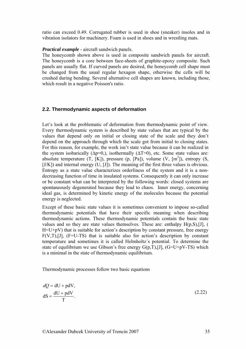
Thermodynamic processes follow two basic equations

.T

pdVdUdS

pdV,dU+

=

+=dQ (2.22)


First equation is called “the first thermodynamic law” and we can understand it as law of thermal energy conservation. The second equation is a thermodynamic form for entropy.

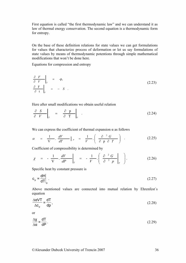
On the base of these definition relations for state values we can get formulations for values that characterize process of deformation or let us say formulations of state values by means of thermodynamic potentions through simple mathematical modifications that won’t be done here.

Equations for compression and entropy

.t

F

-p,

S

VF

V

T

−=∂

∂

=∂∂

(2.23)

Here after small modifications we obtain useful relation

.Tp

VTVS

∂∂

=∂∂ (2.24)

We can express the coefficient of thermal expansion α as follows

⎟⎟⎠

⎞⎜⎜⎝

⎛∂∂

∂==

TG

VdTdV

P p.1.

V1 2

α . (2.25)

Coefficient of compressibility is determined by

..1-.V1- 2 ⎟

⎟⎠

⎞⎜⎜⎝

⎛

∂∂

==TT p

GVdP

dV 2

χ (2.26)

Specific heat by constant pressure is

pp dT

dH=c . (2.27)

Above mentioned values are connected into mutual relation by Ehrenfest´s equation

dpdT

=cVTα

p∆∆

, (2.28)

or

dPdT

=αχ

∆∆

. (2.29)


In conclusion we would like to mention one useful equation to describe compression. This equation is reached by partial derivation of the first thermodynamic law on the base of V and with the use of relation (2.23) and (2.24).

TTp

Vp

VT

.U-∂∂

+∂∂

= . (2.30)

This equation will be later used to derive the basic mechanical properties of rubber.

From the equations mentioned above results that the process of deformation is closely related to thermodynamic state of mechanically stressed system and parameters that described it. As we will see later, for polymer materials the situation describing deformation is more complicated because above mentioned equations are valid for the state of thermodynamic equilibrium.

References [1] http://silver.neep.wisc.edu/~lakes/PoissonIntro.html

[2] Koštial, Pavol: Fyzikálne základy materiálového inžinierstva I - Žilina: ZUSI,

2000, ISBN 80-968278-7-1

Fundamental questions from present part:

13. What are the components of crystalline materials deformation? How would you describe the cause of elastic-reversible deformation from the point of view of elastic substance microstructure?

14. What causes plastic - irreversible deformation in crystals? 15. Write down Hook´s law for isotropic homogeneous solid deformed in

tension or compression. Explain physical significance of the used symbols.

16. Write down law for shear deformation of isotropic homogeneous solid. Explain physical significance of the used symbols.

17. In which SI scale units are modules E and G measured and what do they determine?

18. Explain meaning of Poisson’s number and Poisson’s modulus according to physics. What are their mathematical formulations?

19. What is physically determined non-dimensional deformation presented in relation 2.5.?

γ


CHAPTER 3 Viscosity and mechanical properties of viscous and

viscoelastic materials Objective to achieve This chapter introduces the viscosity terms and viscoelastic behaviour of materials under loading. There is presented the terminology of complex physical parameters (modules), WLF transformations and results of rubber mixtures measurements and temperature dependence of viscosity.

3.1. Viscosity We are going to deal with peculiarities of viscoelastic materials, to which both rubber and polymers belong. We will base on the terminology and the indication of quantities established in the part 3.1. The term viscosity is mostly associated with the liquid and gaseous state. The viscosity is a physical phenomenon caused by Van der Waals’s forces acting among particles of liquid and gas while they are moving. If the movement is only of “sliding” character, then, as we already know from the basic course of physics, the Newton’s viscous law is applied in the following form:

drdν

η=T , (3.1)

where is a tangential tension, η is a dynamic viscosity and v is a flow speed. So we can see that in the material there must be a gradient of the speed of the flow of the consisting particles for using viscous processes. The liquids, whose behaviour is determined by the equation 3.1, we call the Newton’s. However, the real liquids are different from the Newton’s. Also water as relatively less viscous liquid behaves “elastic”, if we, for example, apply high tensions on it in short impulses. We know this phenomenon very well, for example from “unsuccessful jumps” into water, when we fall on our belly (elastic reaction of the water is sufficiently perceptible). The time development of mechanically loaded viscous environment also depends on the duration of acting of the load.

T

In previous considerations, we have dealt only with properties of elastic materials. Real materials, however, always appear within defined conditions as viscous as well. These properties arise from the very character of materials, which are in metastable state (gas, some high-polymeric substance). This phenomenon of the flowing is possible to watch for glass on windows of old churches that run spontaneously under influence of external conditions, what is proved in that way, that glasses are thicker at frames than in the middle. Deformation caused by impressed mechanical tension to steel cause a change of inter-nuclear distances, but in plastic materials there is mainly a change of the valence angle.


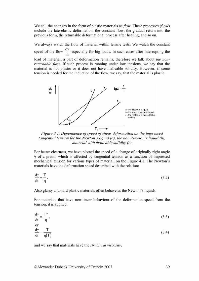
We call the changes in the form of plastic materials as flow. These processes (flow) include the late elastic deformation, the constant flow, the gradual return into the previous form, the returnable deformational process after heating, and so on. We always watch the flow of material within tensile tests. We watch the constant

speed of the flow dtdγ especially for big loads. In such cases after interrupting the

load of material, a part of deformation remains, therefore we talk about the non-returnable flow. If such process is running under low tensions, we say that the material is not plastic or it does not have malleable solidity. However, if some tension is needed for the induction of the flow, we say, that the material is plastic.

Figure 3.1. Dependence of speed of shear deformation on the impressed

tangential tension for the Newton’s liquid (a), the non–Newton’s liquid (b), material with malleable solidity (c)

For better clearness, we have plotted the speed of a change of originally right angle γ of a prism, which is affected by tangential tension as a function of impressed mechanical tension for various types of material, on the Figure 4.1. The Newton’s materials have the deformation speed described with the relation:

η=

γ Tdtd . (3.2)

Also glassy and hard plastic materials often behave as the Newton’s liquids. For materials that have non-linear behaviour of the deformation speed from the tension, it is applied:

η=

γ n

dtd T , (3.3)

or

( )TT

η=

γdtd (3.4)

and we say that materials have the structural viscosity.


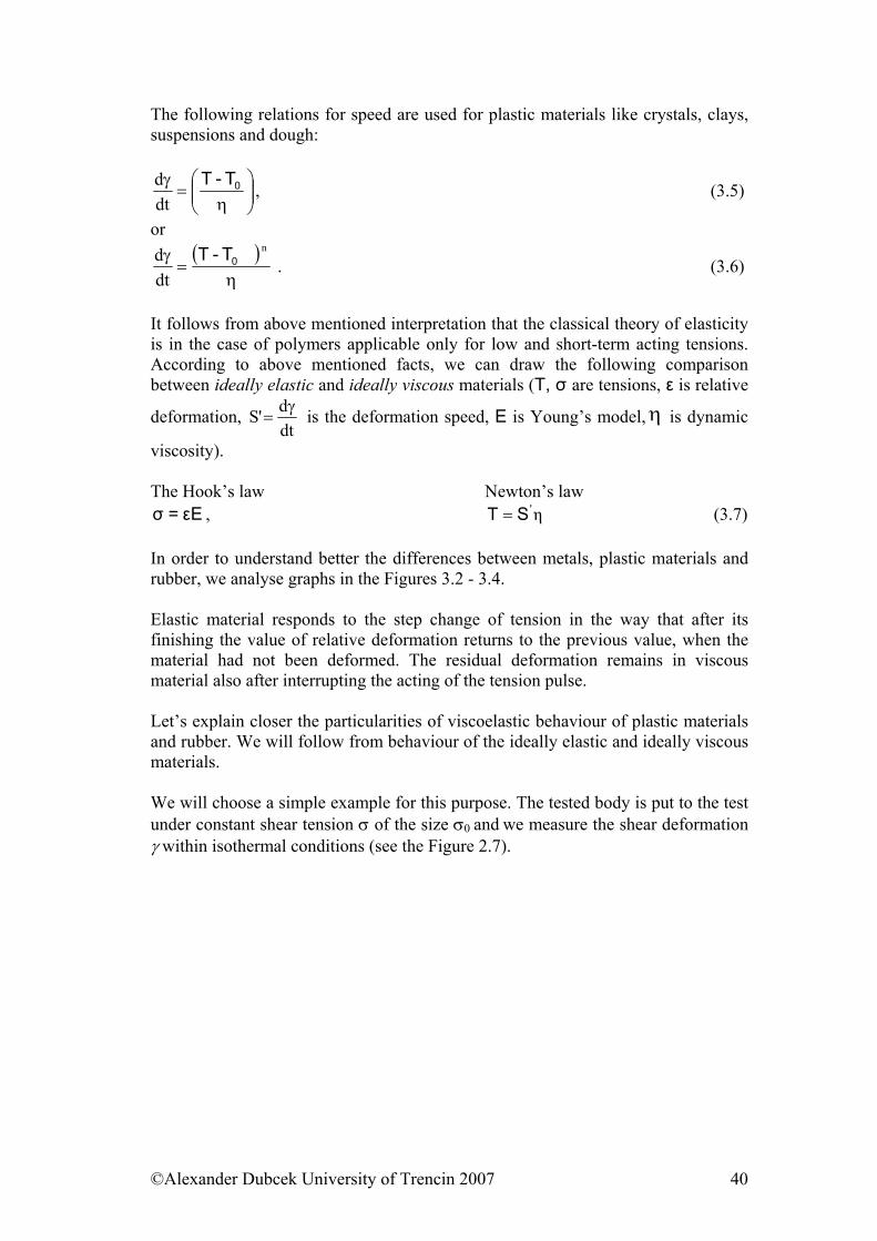
The following relations for speed are used for plastic materials like crystals, clays, suspensions and dough:

⎟⎟⎠

⎞⎜⎜⎝

⎛η

=γ 0T-T

dtd , (3.5)

or ( )

η=

γ n

dtd 0T-T

. (3.6)

It follows from above mentioned interpretation that the classical theory of elasticity is in the case of polymers applicable only for low and short-term acting tensions. According to above mentioned facts, we can draw the following comparison between ideally elastic and ideally viscous materials (T, σ are tensions, ε is relative

deformation, dtd'S γ

= is the deformation speed, E is Young’s model, is dynamic

viscosity).

η

The Hook’s law Newton’s law

Eε=σ , (3.7) η'ST = In order to understand better the differences between metals, plastic materials and rubber, we analyse graphs in the Figures 3.2 - 3.4. Elastic material responds to the step change of tension in the way that after its finishing the value of relative deformation returns to the previous value, when the material had not been deformed. The residual deformation remains in viscous material also after interrupting the acting of the tension pulse. Let’s explain closer the particularities of viscoelastic behaviour of plastic materials and rubber. We will follow from behaviour of the ideally elastic and ideally viscous materials. We will choose a simple example for this purpose. The tested body is put to the test under constant shear tension σ of the size σ0 and we measure the shear deformation γ within isothermal conditions (see the Figure 2.7).


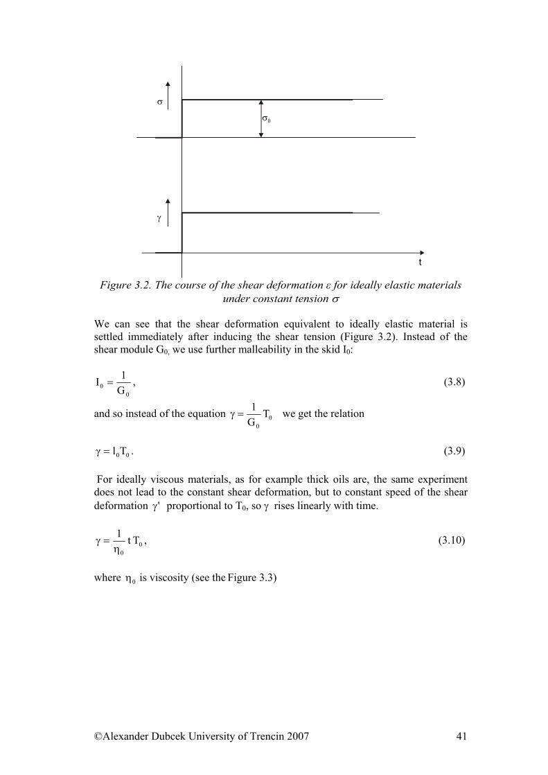
σ

γ

σ0

t

Figure 3.2. The course of the shear deformation ε for ideally elastic materials under constant tension σ

We can see that the shear deformation equivalent to ideally elastic material is settled immediately after inducing the shear tension (Figure 3.2). Instead of the shear module G0, we use further malleability in the skid I0:

00 G

1I = , (3.8)

and so instead of the equation 00

TG1

=γ we get the relation

00Tl=γ . (3.9)

For ideally viscous materials, as for example thick oils are, the same experiment does not lead to the constant shear deformation, but to constant speed of the shear deformation ' proportional to Tγ 0, so γ rises linearly with time.

00

Tt1η

=γ , (3.10)

where 0η is viscosity (see the Figure 3.3)


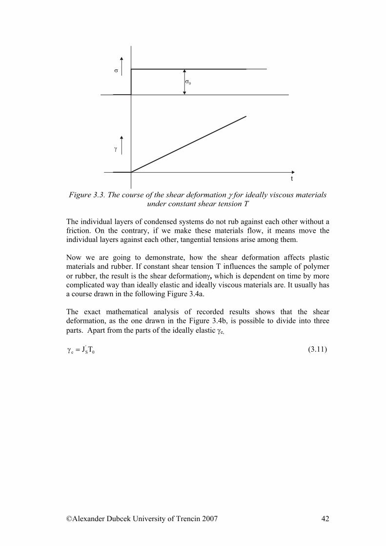
σ

γ

σ0

t

Figure 3.3. The course of the shear deformation γ for ideally viscous materials under constant shear tension T

The individual layers of condensed systems do not rub against each other without a friction. On the contrary, if we make these materials flow, it means move the individual layers against each other, tangential tensions arise among them. Now we are going to demonstrate, how the shear deformation affects plastic materials and rubber. If constant shear tension T influences the sample of polymer or rubber, the result is the shear deformationγ, which is dependent on time by more complicated way than ideally elastic and ideally viscous materials are. It usually has a course drawn in the following Figure 3.4a. The exact mathematical analysis of recorded results shows that the shear deformation, as the one drawn in the Figure 3.4b, is possible to divide into three parts. Apart from the parts of the ideally elastic γe,

0'Se TJ=γ (3.11)


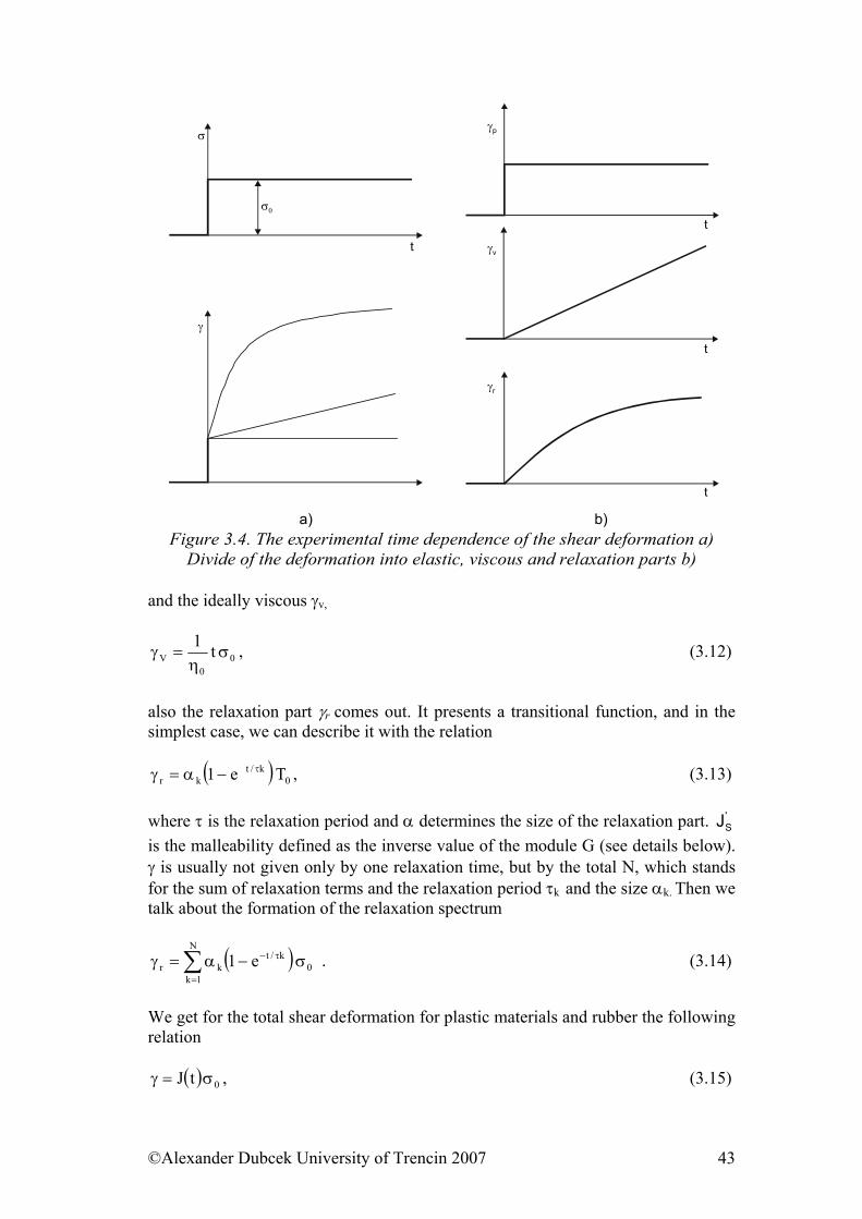
γp

t

t

t

γv

γr

σ

t

γ

σ0

a) b) Figure 3.4. The experimental time dependence of the shear deformation a)

Divide of the deformation into elastic, viscous and relaxation parts b) and the ideally viscous γv,

00

V t1σ

η=γ , (3.12)

also the relaxation part γr comes out. It presents a transitional function, and in the simplest case, we can describe it with the relation

( ) 0k/t

kr Te1 τ−α=γ , (3.13) where τ is the relaxation period and α determines the size of the relaxation part. is the malleability defined as the inverse value of the module G (see details below). γ is usually not given only by one relaxation time, but by the total N, which stands for the sum of relaxation terms and the relaxation period τ

'SJ

k and the size αk. Then we talk about the formation of the relaxation spectrum

( )∑=

τ− σ−α=γN

1k0

k/tkr e1 . (3.14)

We get for the total shear deformation for plastic materials and rubber the following relation

( ) 0tJ σ=γ , (3.15)


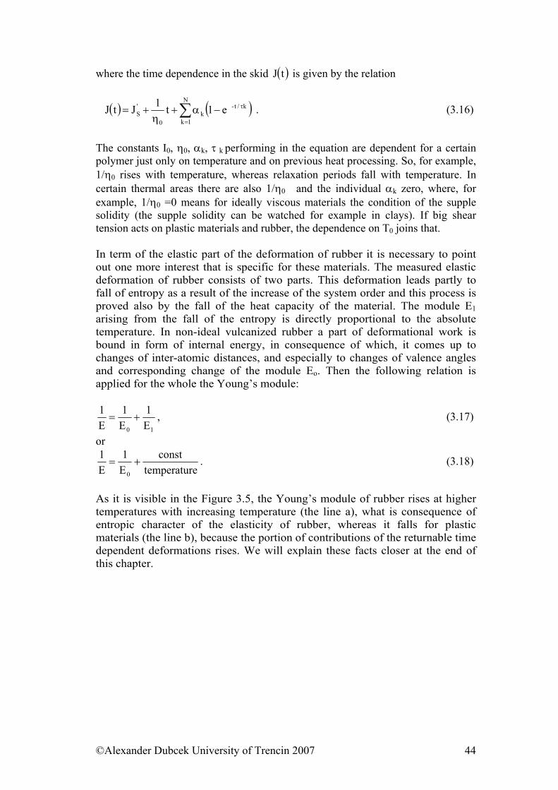
where the time dependence in the skid ( )tJ is given by the relation

( ) ( )∑=

τ−α+η

+=N

1k

k/t-k

0

'S e1t1JtJ . (3.16)

The constants I0, η0, αk, τ k performing in the equation are dependent for a certain polymer just only on temperature and on previous heat processing. So, for example, 1/η0 rises with temperature, whereas relaxation periods fall with temperature. In certain thermal areas there are also 1/η0 and the individual αk zero, where, for example, 1/η0 =0 means for ideally viscous materials the condition of the supple solidity (the supple solidity can be watched for example in clays). If big shear tension acts on plastic materials and rubber, the dependence on T0 joins that. In term of the elastic part of the deformation of rubber it is necessary to point out one more interest that is specific for these materials. The measured elastic deformation of rubber consists of two parts. This deformation leads partly to fall of entropy as a result of the increase of the system order and this process is proved also by the fall of the heat capacity of the material. The module E1 arising from the fall of the entropy is directly proportional to the absolute temperature. In non-ideal vulcanized rubber a part of deformational work is bound in form of internal energy, in consequence of which, it comes up to changes of inter-atomic distances, and especially to changes of valence angles and corresponding change of the module Eo. Then the following relation is applied for the whole the Young’s module:

10 E1

E1

E1

+= , (3.17)

or

etemperaturconst

E1

E1

0

+= . (3.18)

As it is visible in the Figure 3.5, the Young’s module of rubber rises at higher temperatures with increasing temperature (the line a), what is consequence of entropic character of the elasticity of rubber, whereas it falls for plastic materials (the line b), because the portion of contributions of the returnable time dependent deformations rises. We will explain these facts closer at the end of this chapter.


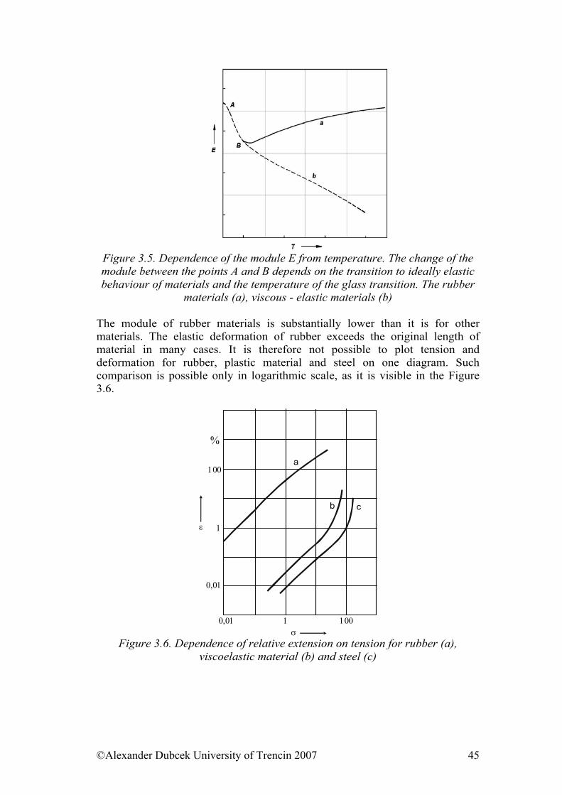
Figure 3.5. Dependence of the module E from temperature. The change of the module between the points A and B depends on the transition to ideally elastic behaviour of materials and the temperature of the glass transition. The rubber

materials (a), viscous - elastic materials (b)

The module of rubber materials is substantially lower than it is for other materials. The elastic deformation of rubber exceeds the original length of material in many cases. It is therefore not possible to plot tension and deformation for rubber, plastic material and steel on one diagram. Such comparison is possible only in logarithmic scale, as it is visible in the Figure 3.6.

%

100

1

0,01

0,01 1 100

a

b c

ε

σ Figure 3.6. Dependence of relative extension on tension for rubber (a),

viscoelastic material (b) and steel (c)


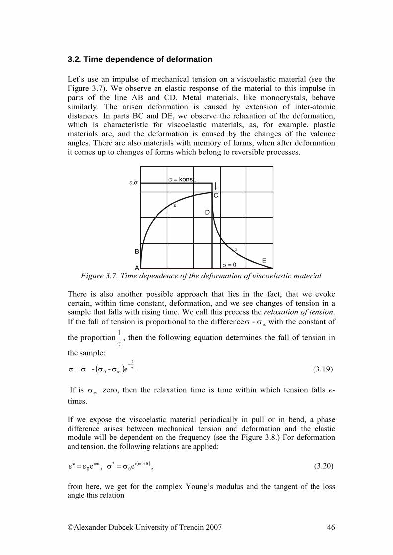
3.2. Time dependence of deformation Let’s use an impulse of mechanical tension on a viscoelastic material (see the Figure 3.7). We observe an elastic response of the material to this impulse in parts of the line AB and CD. Metal materials, like monocrystals, behave similarly. The arisen deformation is caused by extension of inter-atomic distances. In parts BC and DE, we observe the relaxation of the deformation, which is characteristic for viscoelastic materials, as, for example, plastic materials are, and the deformation is caused by the changes of the valence angles. There are also materials with memory of forms, when after deformation it comes up to changes of forms which belong to reversible processes.

σ = 0

ε

ε

ε,σ σ = konst.

C

D

EA

B

Figure 3.7. Time dependence of the deformation of viscoelastic material

There is also another possible approach that lies in the fact, that we evoke certain, within time constant, deformation, and we see changes of tension in a sample that falls with rising time. We call this process the relaxation of tension. If the fall of tension is proportional to the difference ∞σσ - with the constant of

the proportionτ1 , then the following equation determines the fall of tension in

the sample:

( ) τ−

∞σσσ=σt

0 e-- . (3.19) If is zero, then the relaxation time is time within which tension falls e-times.

∞σ

If we expose the viscoelastic material periodically in pull or in bend, a phase difference arises between mechanical tension and deformation and the elastic module will be dependent on the frequency (see the Figure 3.8.) For deformation and tension, the following relations are applied:

( )δ+ωω σ=σε=ε ti0

*ti e,e0* , (3.20) from here, we get for the complex Young’s modulus and the tangent of the loss angle this relation


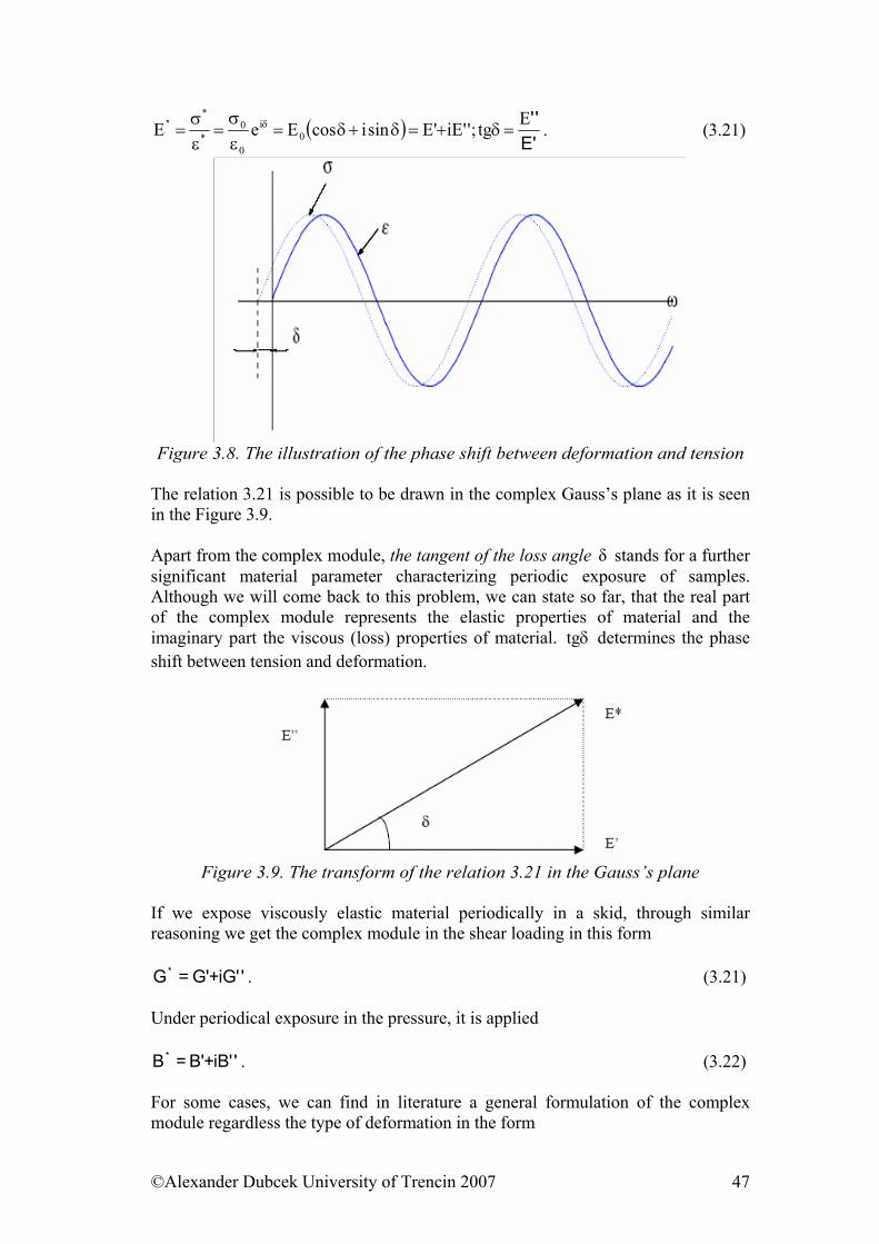
( )E'

''* Etg;''iE'EsinicosEeE 0i

0

0*

*

=δ+=δ+δ=εσ

=εσ

= δ . (3.21)

Figure 3.8. The illustration of the phase shift between deformation and tension

The relation 3.21 is possible to be drawn in the complex Gauss’s plane as it is seen in the Figure 3.9. Apart from the complex module, the tangent of the loss angle δ stands for a further significant material parameter characterizing periodic exposure of samples. Although we will come back to this problem, we can state so far, that the real part of the complex module represents the elastic properties of material and the imaginary part the viscous (loss) properties of material. δtg determines the phase shift between tension and deformation.

Figure 3.9. The transform of the relation 3.21 in the Gauss’s plane

If we expose viscously elastic material periodically in a skid, through similar reasoning we get the complex module in the shear loading in this form

''iG+'G=G* . (3.21) Under periodical exposure in the pressure, it is applied

''iB+'B=B* . (3.22) For some cases, we can find in literature a general formulation of the complex module regardless the type of deformation in the form


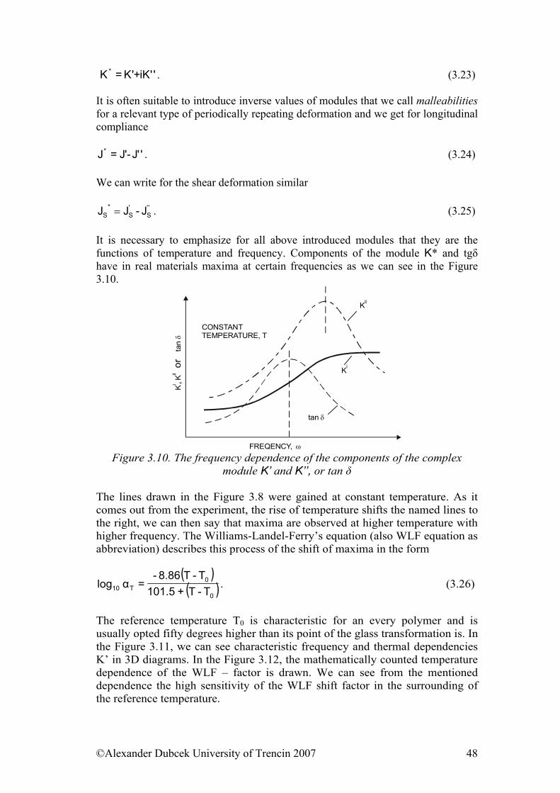
. (3.23) ''iK+'K=K *

It is often suitable to introduce inverse values of modules that we call malleabilities for a relevant type of periodically repeating deformation and we get for longitudinal compliance

''J-'J=J* . (3.24) We can write for the shear deformation similar

''S

'S

*S J-JJ = . (3.25)

It is necessary to emphasize for all above introduced modules that they are the functions of temperature and frequency. Components of the module K* and tgδ have in real materials maxima at certain frequencies as we can see in the Figure 3.10.

tan δ

CONSTANTTEMPERATURE, T

FREQENCY, ω

Kl

Kll

KK

tan

l

ll,

or

δ

Figure 3.10. The frequency dependence of the components of the complex

module K’ and K’’, or tan δ The lines drawn in the Figure 3.8 were gained at constant temperature. As it comes out from the experiment, the rise of temperature shifts the named lines to the right, we can then say that maxima are observed at higher temperature with higher frequency. The Williams-Landel-Ferry’s equation (also WLF equation as abbreviation) describes this process of the shift of maxima in the form

( )( )0

0T10 T-T+101.5

T-T8.86-=αlog . (3.26)

The reference temperature T0 is characteristic for an every polymer and is usually opted fifty degrees higher than its point of the glass transformation is. In the Figure 3.11, we can see characteristic frequency and thermal dependencies K’ in 3D diagrams. In the Figure 3.12, the mathematically counted temperature dependence of the WLF – factor is drawn. We can see from the mentioned dependence the high sensitivity of the WLF shift factor in the surrounding of the reference temperature.


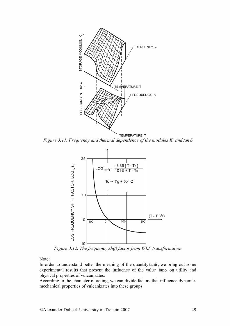
FREQUENCY, ω

TEMPERATURE, T

FREQUENCY, ω

TEMPERATURE, T

LOS

S T

AN

GE

NT,

tan

δS

TOR

AG

E M

OD

ULU

S,

Kl

Figure 3.11. Frequency and thermal dependence of the modules K’ and tan δ

LOG

FR

EQ

UE

NC

Y S

HIF

T FA

CTO

R, L

OG

a10

T

LOG a =10 T- 8 86 [ T - T ]o ⋅

To ∼ Τg + 50 C°

(T - T ) Co °-100 100 2000

-10

10

0

25

Figure 3.12. The frequency shift factor from WLF transformation

Note: In order to understand better the meaning of the quantity , we bring out some experimental results that present the influence of the value on utility and physical properties of vulcanizates.

tanδtanδ

According to the character of acting, we can divide factors that influence dynamic- mechanical properties of vulcanizates into these groups:


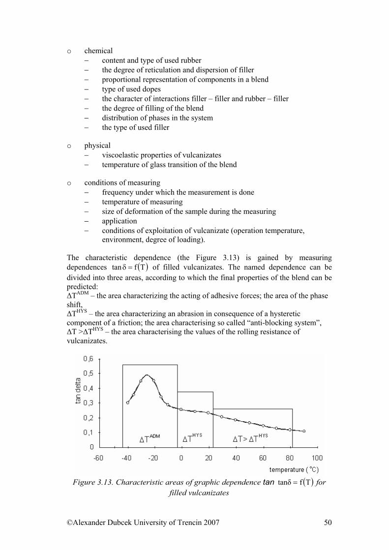
o chemical − content and type of used rubber − the degree of reticulation and dispersion of filler − proportional representation of components in a blend − type of used dopes − the character of interactions filler – filler and rubber – filler − the degree of filling of the blend − distribution of phases in the system − the type of used filler

o physical

− viscoelastic properties of vulcanizates − temperature of glass transition of the blend

o conditions of measuring

− frequency under which the measurement is done − temperature of measuring − size of deformation of the sample during the measuring − application − conditions of exploitation of vulcanizate (operation temperature,

environment, degree of loading). The characteristic dependence (the Figure 3.13) is gained by measuring dependences of filled vulcanizates. The named dependence can be divided into three areas, according to which the final properties of the blend can be predicted:

( )Tftan =δ

∆TADM – the area characterizing the acting of adhesive forces; the area of the phase shift, ∆THYS – the area characterizing an abrasion in consequence of a hysteretic component of a friction; the area characterising so called “anti-blocking system”, ∆T >∆THYS – the area characterising the values of the rolling resistance of vulcanizates.

Figure 3.13. Characteristic areas of graphic dependence tan for

filled vulcanizates ( )Tftanδ =


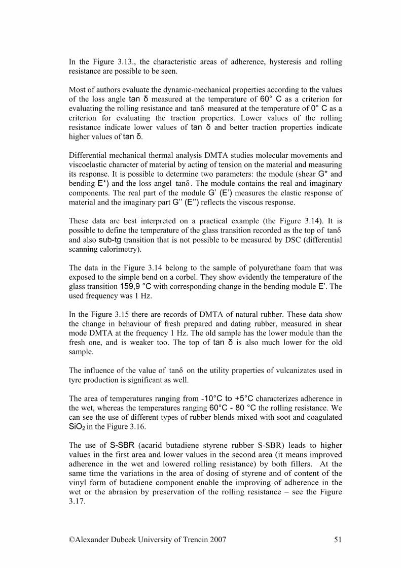
In the Figure 3.13., the characteristic areas of adherence, hysteresis and rolling resistance are possible to be seen. Most of authors evaluate the dynamic-mechanical properties according to the values of the loss angle tan δ measured at the temperature of 60° C as a criterion for evaluating the rolling resistance and measured at the temperature of 0° C as a criterion for evaluating the traction properties. Lower values of the rolling resistance indicate lower values of tan δ and better traction properties indicate higher values of tan δ.

tanδ

Differential mechanical thermal analysis DMTA studies molecular movements and viscoelastic character of material by acting of tension on the material and measuring its response. It is possible to determine two parameters: the module (shear G* and bending E*) and the loss angel . The module contains the real and imaginary components. The real part of the module G’ (E’) measures the elastic response of material and the imaginary part G’’ (E’’) reflects the viscous response.

tanδ

These data are best interpreted on a practical example (the Figure 3.14). It is possible to define the temperature of the glass transition recorded as the top of and also sub-tg transition that is not possible to be measured by DSC (differential scanning calorimetry).

tanδ

The data in the Figure 3.14 belong to the sample of polyurethane foam that was exposed to the simple bend on a corbel. They show evidently the temperature of the glass transition 159,9 °C with corresponding change in the bending module E’. The used frequency was 1 Hz. In the Figure 3.15 there are records of DMTA of natural rubber. These data show the change in behaviour of fresh prepared and dating rubber, measured in shear mode DMTA at the frequency 1 Hz. The old sample has the lower module than the fresh one, and is weaker too. The top of tan δ is also much lower for the old sample. The influence of the value of on the utility properties of vulcanizates used in tyre production is significant as well.

tanδ

The area of temperatures ranging from -10°C to +5°C characterizes adherence in the wet, whereas the temperatures ranging 60°C - 80 °C the rolling resistance. We can see the use of different types of rubber blends mixed with soot and coagulated SiO2 in the Figure 3.16. The use of S-SBR (acarid butadiene styrene rubber S-SBR) leads to higher values in the first area and lower values in the second area (it means improved adherence in the wet and lowered rolling resistance) by both fillers. At the same time the variations in the area of dosing of styrene and of content of the vinyl form of butadiene component enable the improving of adherence in the wet or the abrasion by preservation of the rolling resistance – see the Figure 3.17.


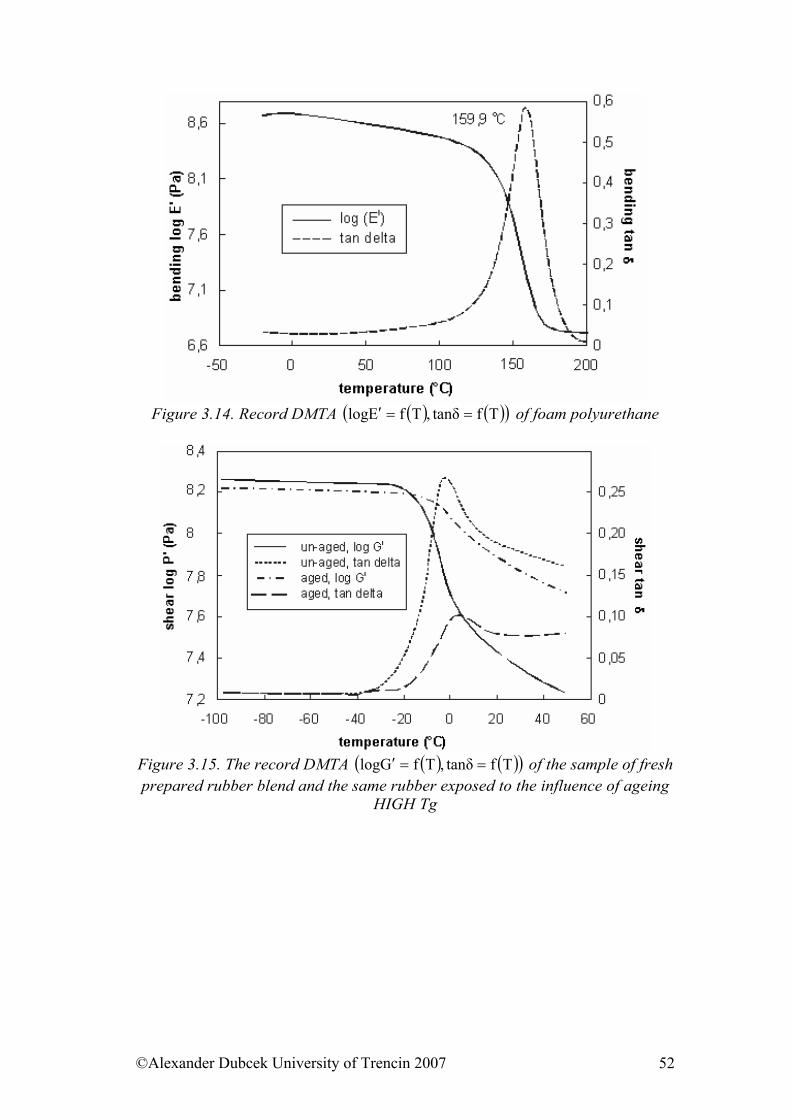
Figure 3.14. Record DMTA ( ) ( )( )Tftanδ,TfElog ==′ of foam polyurethane

Figure 3.15. The record DMTA ( ) ( )( )Tftanδ,TfGlog ==′ of the sample of fresh prepared rubber blend and the same rubber exposed to the influence of ageing

HIGH Tg


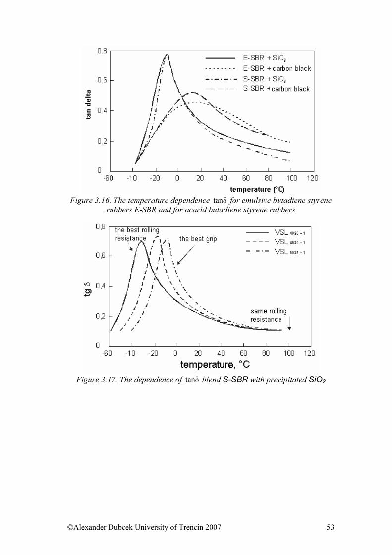
Figure 3.16. The temperature dependence for emulsive butadiene styrene

rubbers E-SBR and for acarid butadiene styrene rubbers tanδ

Figure 3.17. The dependence of blend S-SBR with precipitated SiOtanδ 2


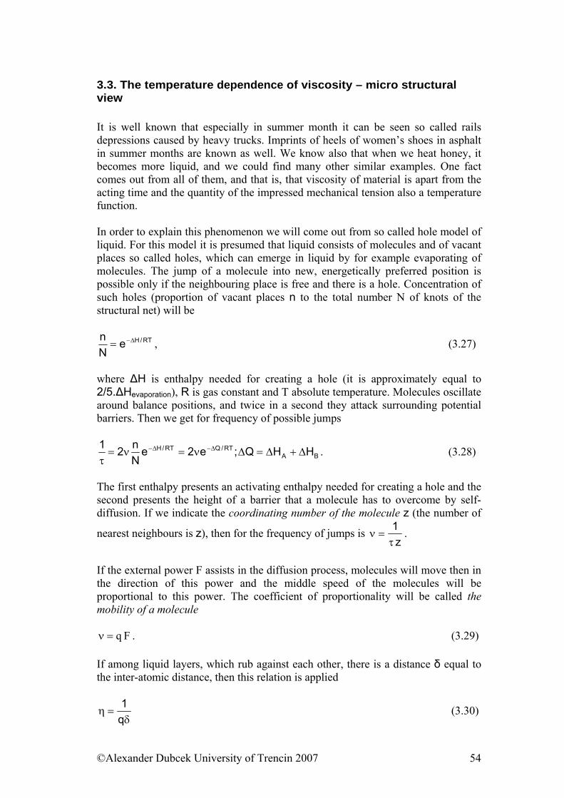
3.3. The temperature dependence of viscosity – micro structural view It is well known that especially in summer month it can be seen so called rails depressions caused by heavy trucks. Imprints of heels of women’s shoes in asphalt in summer months are known as well. We know also that when we heat honey, it becomes more liquid, and we could find many other similar examples. One fact comes out from all of them, and that is, that viscosity of material is apart from the acting time and the quantity of the impressed mechanical tension also a temperature function. In order to explain this phenomenon we will come out from so called hole model of liquid. For this model it is presumed that liquid consists of molecules and of vacant places so called holes, which can emerge in liquid by for example evaporating of molecules. The jump of a molecule into new, energetically preferred position is possible only if the neighbouring place is free and there is a hole. Concentration of such holes (proportion of vacant places n to the total number N of knots of the structural net) will be

RT/HeNn ∆−= , (3.27)

where ∆H is enthalpy needed for creating a hole (it is approximately equal to 2/5.∆Hevaporation), R is gas constant and T absolute temperature. Molecules oscillate around balance positions, and twice in a second they attack surrounding potential barriers. Then we get for frequency of possible jumps

BART/QRT/H HHQ;e2e

Nn21

∆+∆=∆ν=ν=τ

∆−∆− . (3.28)

The first enthalpy presents an activating enthalpy needed for creating a hole and the second presents the height of a barrier that a molecule has to overcome by self-diffusion. If we indicate the coordinating number of the molecule z (the number of

nearest neighbours is z), then for the frequency of jumps is z

1τ

=ν .

If the external power F assists in the diffusion process, molecules will move then in the direction of this power and the middle speed of the molecules will be proportional to this power. The coefficient of proportionality will be called the mobility of a molecule

Fq=ν . (3.29) If among liquid layers, which rub against each other, there is a distance δ equal to the inter-atomic distance, then this relation is applied

δ=η

q1 (3.30)


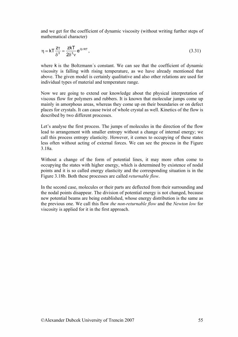
and we get for the coefficient of dynamic viscosity (without writing further steps of mathematical character)

RT/Q33 e

2zkTzkT

νδ=

δτ

=η , (3.31)

where k is the Boltzmann´s constant. We can see that the coefficient of dynamic viscosity is falling with rising temperature, as we have already mentioned that above. The given model is certainly qualitative and also other relations are used for individual types of material and temperature range. Now we are going to extend our knowledge about the physical interpretation of viscous flow for polymers and rubbers. It is known that molecular jumps come up mainly in amorphous areas, whereas they come up on their boundaries or on defect places for crystals. It can cause twist of whole crystal as well. Kinetics of the flow is described by two different processes. Let’s analyse the first process. The jumps of molecules in the direction of the flow lead to arrangement with smaller entropy without a change of internal energy; we call this process entropy elasticity. However, it comes to occupying of these states less often without acting of external forces. We can see the process in the Figure 3.18a. Without a change of the form of potential lines, it may more often come to occupying the states with higher energy, which is determined by existence of nodal points and it is so called energy elasticity and the corresponding situation is in the Figure 3.18b. Both these processes are called returnable flow. In the second case, molecules or their parts are deflected from their surrounding and the nodal points disappear. The division of potential energy is not changed, because new potential beams are being established, whose energy distribution is the same as the previous one. We call this flow the non-returnable flow and the Newton low for viscosity is applied for it in the first approach.


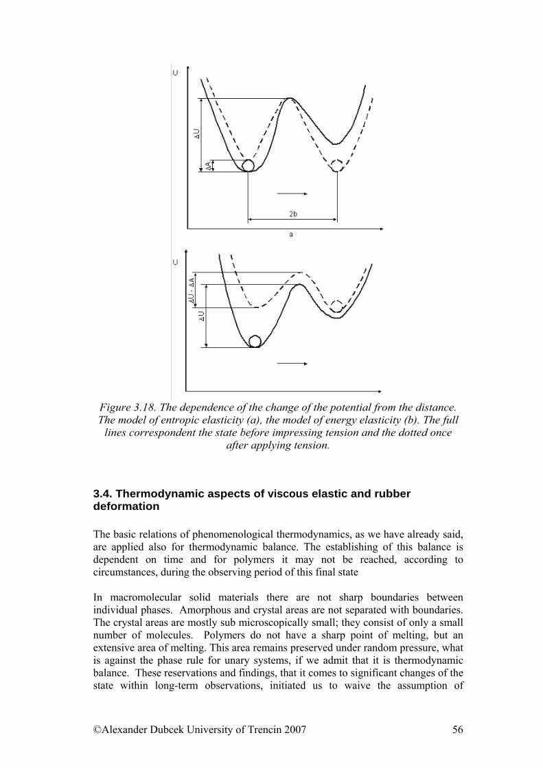
Figure 3.18. The dependence of the change of the potential from the distance. The model of entropic elasticity (a), the model of energy elasticity (b). The full

lines correspondent the state before impressing tension and the dotted once after applying tension.

3.4. Thermodynamic aspects of viscous elastic and rubber deformation The basic relations of phenomenological thermodynamics, as we have already said, are applied also for thermodynamic balance. The establishing of this balance is dependent on time and for polymers it may not be reached, according to circumstances, during the observing period of this final state In macromolecular solid materials there are not sharp boundaries between individual phases. Amorphous and crystal areas are not separated with boundaries. The crystal areas are mostly sub microscopically small; they consist of only a small number of molecules. Polymers do not have a sharp point of melting, but an extensive area of melting. This area remains preserved under random pressure, what is against the phase rule for unary systems, if we admit that it is thermodynamic balance. These reservations and findings, that it comes to significant changes of the state within long-term observations, initiated us to waive the assumption of


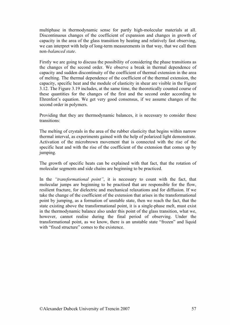
multiphase in thermodynamic sense for partly high-molecular materials at all. Discontinuous changes of the coefficient of expansion and changes in growth of capacity in the area of the glass transition by heating and relatively fast observing, we can interpret with help of long-term measurements in that way, that we call them non-balanced state. Firstly we are going to discuss the possibility of considering the phase transitions as the changes of the second order. We observe a break in thermal dependence of capacity and sudden discontinuity of the coefficient of thermal extension in the area of melting. The thermal dependence of the coefficient of the thermal extension, the capacity, specific heat and the module of elasticity in shear are visible in the Figure 3.12. The Figure 3.19 includes, at the same time, the theoretically counted course of these quantities for the changes of the first and the second order according to Ehrenfest’s equation. We get very good consensus, if we assume changes of the second order in polymers. Providing that they are thermodynamic balances, it is necessary to consider these transitions: The melting of crystals in the area of the rubber elasticity that begins within narrow thermal interval, as experiments gained with the help of polarized light demonstrate. Activation of the microbrown movement that is connected with the rise of the specific heat and with the rise of the coefficient of the extension that comes up by jumping. The growth of specific heats can be explained with that fact, that the rotation of molecular segments and side chains are beginning to be practiced. In the “transformational point”, it is necessary to count with the fact, that molecular jumps are beginning to be practised that are responsible for the flow, resilient fracture, for dielectric and mechanical relaxations and for diffusion. If we take the change of the coefficient of the extension that arises in the transformational point by jumping, as a formation of unstable state, then we reach the fact, that the state existing above the transformational point, it is a single-phase melt, must exist in the thermodynamic balance also under this point of the glass transition, what we, however, cannot realise during the final period of observing. Under the transformational point, as we know, there is an unstable state “frozen” and liquid with “fixed structure” comes to the existence.


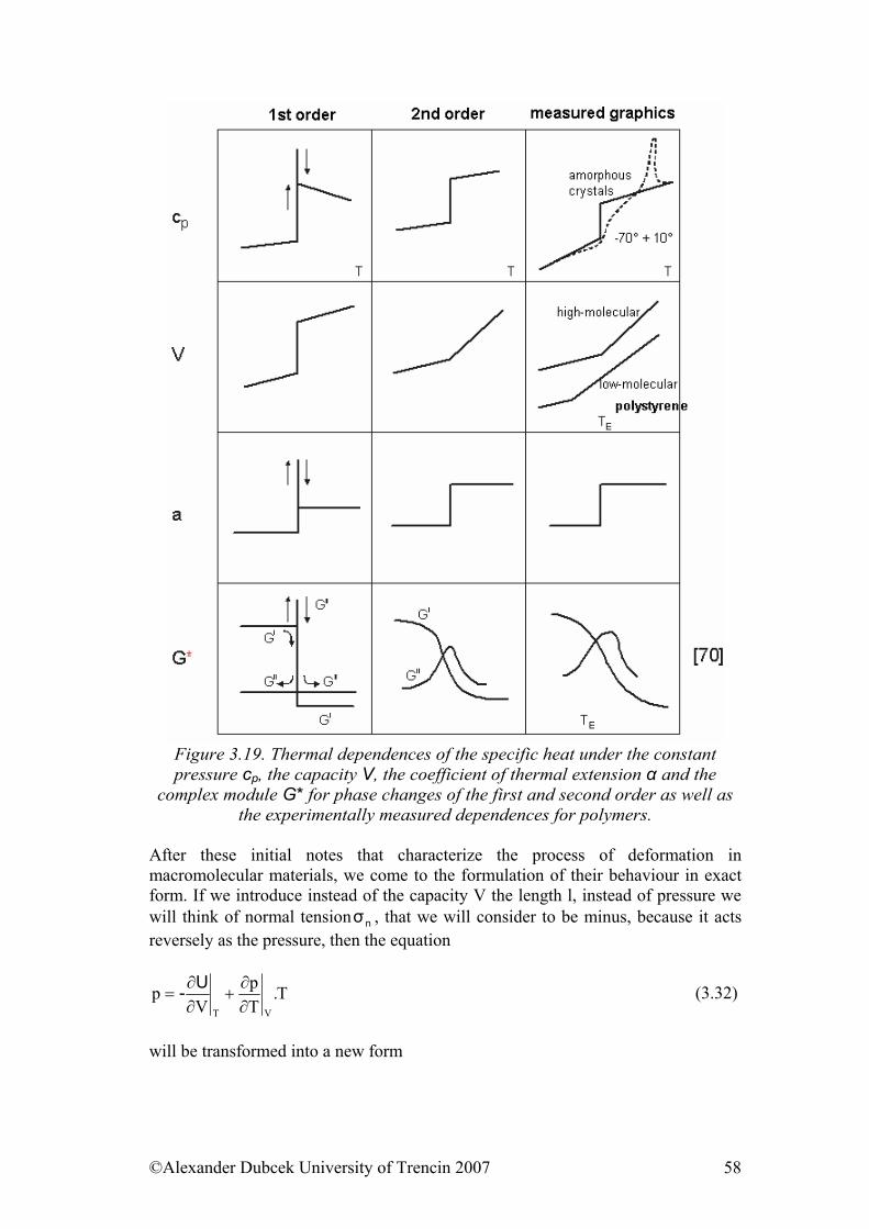
Figure 3.19. Thermal dependences of the specific heat under the constant pressure cp, the capacity V, the coefficient of thermal extension α and the

complex module G* for phase changes of the first and second order as well as the experimentally measured dependences for polymers.

After these initial notes that characterize the process of deformation in macromolecular materials, we come to the formulation of their behaviour in exact form. If we introduce instead of the capacity V the length l, instead of pressure we will think of normal tension , that we will consider to be minus, because it acts reversely as the pressure, then the equation

nσ

T.Tp

Vp

VT ∂∂

+∂∂

=U- (3.32)

will be transformed into a new form


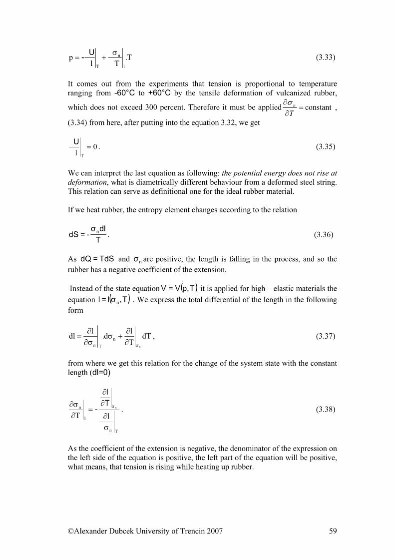
T.Tl

pl

n

T

σ+=

U- (3.33)

It comes out from the experiments that tension is proportional to temperature ranging from -60°C to +60°C by the tensile deformation of vulcanized rubber,

which does not exceed 300 percent. Therefore it must be applied constant =∂∂

Tnσ ,

(3.34) from here, after putting into the equation 3.32, we get

0l T

=U . (3.35)

We can interpret the last equation as following: the potential energy does not rise at deformation, what is diametrically different behaviour from a deformed steel string. This relation can serve as definitional one for the ideal rubber material. If we heat rubber, the entropy element changes according to the relation

Tdlσ

-=dS n . (3.36)

As and are positive, the length is falling in the process, and so the rubber has a negative coefficient of the extension.

TdS=dQ nσ

Instead of the state equation ( )Tp,V=V it is applied for high – elastic materials the equation ( )T,σl=l n . We express the total differential of the length in the following form

dTTld.ldl

n

nTn σ∂

∂+σ

σ∂∂

= , (3.37)

from where we get this relation for the change of the system state with the constant length (dl=0)

Tn

l

n

lTn

σ∂

∂∂

=∂σ∂ σT

l

- . (3.38)

As the coefficient of the extension is negative, the denominator of the expression on the left side of the equation is positive, the left part of the equation will be positive, what means, that tension is rising while heating up rubber.


The deformation in pull leads to the state with higher molecular arrangement, and thus with lower entropy. The thermal flow acts in the sense of renewal of the

previous disordered, that is non-deformed, state. AsT

dQ=dS , the system gives

heat to environment by tensile deformation. If this is not possible, as a consequence, the increase of molecular movements comes up. This adiabatic deformation of rubber results not only in increase of temperature, but also in a bigger growth of tension against the deformation within the constant temperature. This similarity with gas seems to be remarkable, however, it come out from the basic laws of phenomenological thermodynamics.

3.5. Payne effect Various interfering processes occur at cyclical application of stress on polymer material, as was mentioned in chapter 3. The most important of these is superposition of Hooke's deformation of polymer string segments at small amplitude of cyclical deformation on one hand, and translation motion of molecules on the other hand. Result is time delay of deformation after stress by a time period that is at invariable conditions (temperature, frequency and amplitude of deformation) constant. If we systematically increase temperature (or frequency) during the experiment, we can determine conditions when release of certain motion types of string parts occur and determine whole relaxation spectrum of polymer, whereby the most important information is temperature of glassy transition. If we modify conditions of experiment based on cyclical deformation, we can also use the method for characterization of composites, e.g. rubber or plastic filled with active filler. In this case we stabilize experiment conditions what regards temperature and frequency and we change amplitude of deformation. This procedure is based on the principle of so-called Payne effect. Payne effect is in professional literature sometimes referred to as model of variable mesh density. Mesh density is defined as number of cross-links in unit volume of cross-linked polymer. Cross links can be in the polymer of clearly chemical, mostly covalent character, e.g. sulphur bridges in the case of vulcanized rubber, or carbon-carbon bonds at cross-linking of polyolefins, or they can be physical, if strings are in the course of chemical grid creation interconnected e.g. into cycles and create so-called tang lings. The situation is much more complicated when the filler is present, because another space interconnection is created via stable macromolecule attachments on the filler surface, or less stable interactions between polymer segments and filler surface. Finally, even space formations only from filler elements could be formed at filler volume increase. They form firmer or looser interconnected filler elements. Mesh density of vulcanizate is then given by total sum of all mentioned possibilities and its relation to mechanical properties can be modelled by Mooney – Rivlin equation


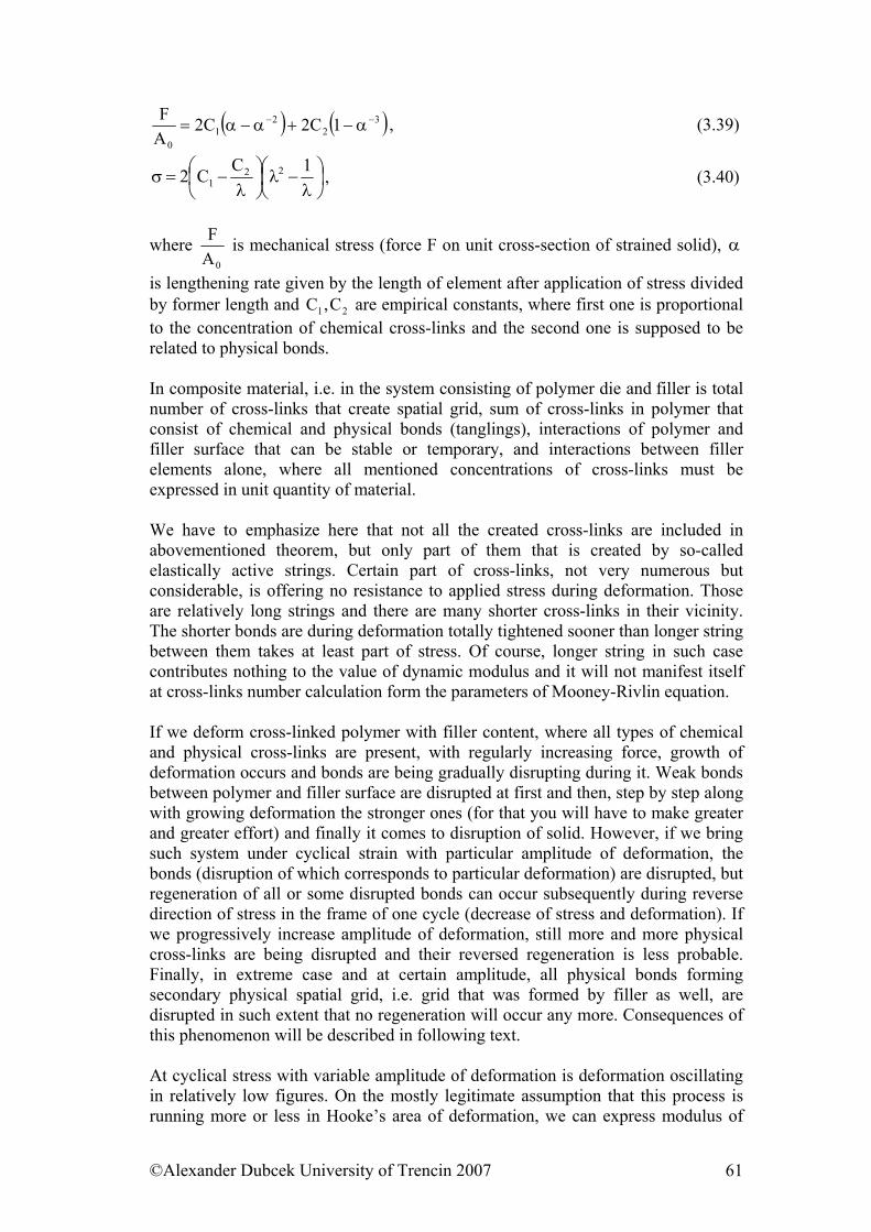
( ) ( 32

21

0

1C2C2AF −− α−+α−α= ), (3.39)

⎟⎠⎞

⎜⎝⎛

λ−λ⎟

⎠⎞

⎜⎝⎛

λ−=σ

1CC2 221 , (3.40)

where 0A

F is mechanical stress (force F on unit cross-section of strained solid), α

is lengthening rate given by the length of element after application of stress divided by former length and are empirical constants, where first one is proportional to the concentration of chemical cross-links and the second one is supposed to be related to physical bonds.

21 C,C

In composite material, i.e. in the system consisting of polymer die and filler is total number of cross-links that create spatial grid, sum of cross-links in polymer that consist of chemical and physical bonds (tanglings), interactions of polymer and filler surface that can be stable or temporary, and interactions between filler elements alone, where all mentioned concentrations of cross-links must be expressed in unit quantity of material. We have to emphasize here that not all the created cross-links are included in abovementioned theorem, but only part of them that is created by so-called elastically active strings. Certain part of cross-links, not very numerous but considerable, is offering no resistance to applied stress during deformation. Those are relatively long strings and there are many shorter cross-links in their vicinity. The shorter bonds are during deformation totally tightened sooner than longer string between them takes at least part of stress. Of course, longer string in such case contributes nothing to the value of dynamic modulus and it will not manifest itself at cross-links number calculation form the parameters of Mooney-Rivlin equation. If we deform cross-linked polymer with filler content, where all types of chemical and physical cross-links are present, with regularly increasing force, growth of deformation occurs and bonds are being gradually disrupting during it. Weak bonds between polymer and filler surface are disrupted at first and then, step by step along with growing deformation the stronger ones (for that you will have to make greater and greater effort) and finally it comes to disruption of solid. However, if we bring such system under cyclical strain with particular amplitude of deformation, the bonds (disruption of which corresponds to particular deformation) are disrupted, but regeneration of all or some disrupted bonds can occur subsequently during reverse direction of stress in the frame of one cycle (decrease of stress and deformation). If we progressively increase amplitude of deformation, still more and more physical cross-links are being disrupted and their reversed regeneration is less probable. Finally, in extreme case and at certain amplitude, all physical bonds forming secondary physical spatial grid, i.e. grid that was formed by filler as well, are disrupted in such extent that no regeneration will occur any more. Consequences of this phenomenon will be described in following text. At cyclical stress with variable amplitude of deformation is deformation oscillating in relatively low figures. On the mostly legitimate assumption that this process is running more or less in Hooke’s area of deformation, we can express modulus of


elasticity as the proportion of stress to amplitude of cyclical deformations. If we regularly increase amplitude (i.e. deformation), we have to proportionally increase stress as well until deformation is increased in such a way that disruption of some grid element occurs. If we achieve total regeneration of disrupted grid at cyclical stress release, the same modulus will be measured in next cycle as if the physical grid has not been disrupted. However, another situation occurs when deformation is so large that whole grid could not manage to regenerate reversibly to its original state. Then, particular deformation (that is constant at cyclical stress) in next cycle is achieved with lesser exerted force, what results in lower values of modulus of elasticity. If we regularly increase the amplitude, then in extreme case we get the state, when specified dynamic modulus will be identical to the modulus of unfilled cross-linked rubber. In this case the whole physical grid is at specific amplitude so much disrupted that its regeneration will practically never happen. We can get this state by increasing the amplitude, while cyclical deformation frequency increase leads to decrease of deformation, at which we observe decrease of dynamic modulus of elasticity. Of course, increase in frequency leaves less time for grid regeneration and it will not manage to regenerate, not even in the case, when its disruption happens in reduced extent with lesser deformation. These reasoning imply the interpretation for observed phenomena that we call Payne effect. When we increase the grade of dynamic deformation, values of modulus of elasticity (E’) for unfilled vulcanizates do not change significantly. But there is modulus decrease in the case of filled vulcanizates, while this effect is more significant for vulcanizates with high filler density. While difference of modulus values is small for unfilled/filled vulcanizate at large deformations and it is relatively high at small deformations, Payne effect is related mostly, if not exclusively, to the grid created by elements of filler in polymer die. Polymer trapped in such grid looses its identity and behaves as filler. Along with increase of filler share in the system, there is increase in effective volume of filler and modulus as well. If higher grade of deformation is applied, disruption of grid created by filler elements occurs and is accompanied by release of polymer that was formerly bound to filler. Effective filler volume (in dynamic process it represents real filler volume increased by the volume of bound immobilized polymer) is by this action decreased, released polymer gets back its former properties and decrease of elastic modulus follows. This implies that Payne effect can be used for characterization of grid formed by filler that comes from filler-filler and filler-polymer interaction. In the case of loss modulus (E’’), like at modulus of elasticity, we observe increase of its values along with rising degree of polymer filling in bundle of dynamic deformations. However in dependence on deformation increase, no monotonous decrease of values occurs (like in the case of modulus of elasticity), but we observe maximum at particular deformation that is characteristic for specific pair of polymer-filler. We assume that process of loss modulus is controlled by disruption and re-creation of grid from filler elements. It implies that loss modulus is dependent on rate of disruption and re-creation of the grid. Rate of disruption and re-creation of the grid emerges from the phenomenon of dynamic deformation alone. Disruption of the grid is considerable at large deformation and its reversed re-creation practically does not happen. If deformation is large enough for the grid not to re-create at specific frequency, influence of the grid on loss modulus will be eliminated. Similarly, if deformation is small (or grid is firm enough) to cause


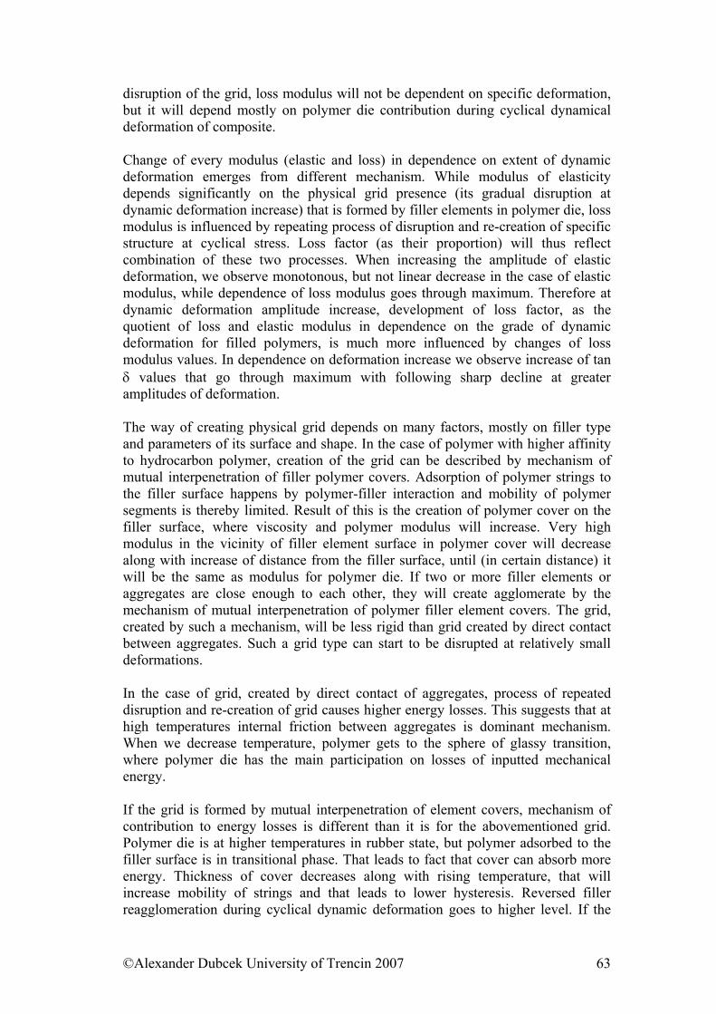
disruption of the grid, loss modulus will not be dependent on specific deformation, but it will depend mostly on polymer die contribution during cyclical dynamical deformation of composite. Change of every modulus (elastic and loss) in dependence on extent of dynamic deformation emerges from different mechanism. While modulus of elasticity depends significantly on the physical grid presence (its gradual disruption at dynamic deformation increase) that is formed by filler elements in polymer die, loss modulus is influenced by repeating process of disruption and re-creation of specific structure at cyclical stress. Loss factor (as their proportion) will thus reflect combination of these two processes. When increasing the amplitude of elastic deformation, we observe monotonous, but not linear decrease in the case of elastic modulus, while dependence of loss modulus goes through maximum. Therefore at dynamic deformation amplitude increase, development of loss factor, as the quotient of loss and elastic modulus in dependence on the grade of dynamic deformation for filled polymers, is much more influenced by changes of loss modulus values. In dependence on deformation increase we observe increase of tan δ values that go through maximum with following sharp decline at greater amplitudes of deformation. The way of creating physical grid depends on many factors, mostly on filler type and parameters of its surface and shape. In the case of polymer with higher affinity to hydrocarbon polymer, creation of the grid can be described by mechanism of mutual interpenetration of filler polymer covers. Adsorption of polymer strings to the filler surface happens by polymer-filler interaction and mobility of polymer segments is thereby limited. Result of this is the creation of polymer cover on the filler surface, where viscosity and polymer modulus will increase. Very high modulus in the vicinity of filler element surface in polymer cover will decrease along with increase of distance from the filler surface, until (in certain distance) it will be the same as modulus for polymer die. If two or more filler elements or aggregates are close enough to each other, they will create agglomerate by the mechanism of mutual interpenetration of polymer filler element covers. The grid, created by such a mechanism, will be less rigid than grid created by direct contact between aggregates. Such a grid type can start to be disrupted at relatively small deformations. In the case of grid, created by direct contact of aggregates, process of repeated disruption and re-creation of grid causes higher energy losses. This suggests that at high temperatures internal friction between aggregates is dominant mechanism. When we decrease temperature, polymer gets to the sphere of glassy transition, where polymer die has the main participation on losses of inputted mechanical energy. If the grid is formed by mutual interpenetration of element covers, mechanism of contribution to energy losses is different than it is for the abovementioned grid. Polymer die is at higher temperatures in rubber state, but polymer adsorbed to the filler surface is in transitional phase. That leads to fact that cover can absorb more energy. Thickness of cover decreases along with rising temperature, that will increase mobility of strings and that leads to lower hysteresis. Reversed filler reagglomeration during cyclical dynamic deformation goes to higher level. If the


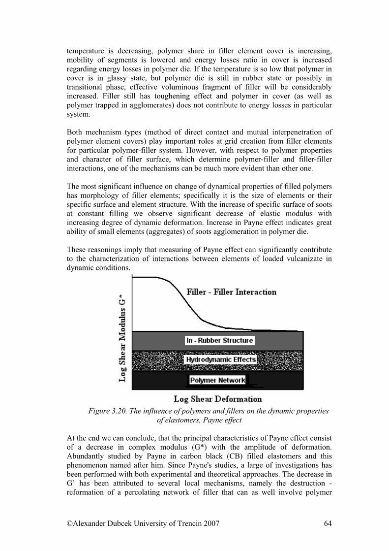
temperature is decreasing, polymer share in filler element cover is increasing, mobility of segments is lowered and energy losses ratio in cover is increased regarding energy losses in polymer die. If the temperature is so low that polymer in cover is in glassy state, but polymer die is still in rubber state or possibly in transitional phase, effective voluminous fragment of filler will be considerably increased. Filler still has toughening effect and polymer in cover (as well as polymer trapped in agglomerates) does not contribute to energy losses in particular system. Both mechanism types (method of direct contact and mutual interpenetration of polymer element covers) play important roles at grid creation from filler elements for particular polymer-filler system. However, with respect to polymer properties and character of filler surface, which determine polymer-filler and filler-filler interactions, one of the mechanisms can be much more evident than other one. The most significant influence on change of dynamical properties of filled polymers has morphology of filler elements; specifically it is the size of elements or their specific surface and element structure. With the increase of specific surface of soots at constant filling we observe significant decrease of elastic modulus with increasing degree of dynamic deformation. Increase in Payne effect indicates great ability of small elements (aggregates) of soots agglomeration in polymer die. These reasonings imply that measuring of Payne effect can significantly contribute to the characterization of interactions between elements of loaded vulcanizate in dynamic conditions.

Figure 3.20. The influence of polymers and fillers on the dynamic properties

of elastomers, Payne effect

At the end we can conclude, that the principal characteristics of Payne effect consist of a decrease in complex modulus (G*) with the amplitude of deformation. Abundantly studied by Payne in carbon black (CB) filled elastomers and this phenomenon named after him. Since Payne's studies, a large of investigations has been performed with both experimental and theoretical approaches. The decrease in G’ has been attributed to several local mechanisms, namely the destruction - reformation of a percolating network of filler that can as well involve polymer


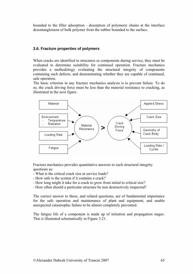
bounded to the filler adsorption - desorption of polymeric chains at the interface desentanglement of bulk polymer from the rubber bounded to the surface.

3.6. Fracture properties of polymers

When cracks are identified in structures or components during service, they must be evaluated to determine suitability for continued operation. Fracture mechanics provides a methodology evaluating the structural integrity of components containing such defects, and demonstrating whether they are capable of continued, safe operation. The basic criterion in any fracture mechanics analysis is to prevent failure. To do so, the crack driving force must be less than the material resistance to cracking, as illustrated in the next figure.

Fracture mechanics provides quantitative answers to such structural integrity questions as: - What is the critical crack size at service loads? - How safe is the system if it contains a crack? - How long might it take for a crack to grow from initial to critical size? - How often should a particular structure be non destructively inspected? The correct answer to these, and related questions, are of fundamental importance for the safe operation and maintenance of plant and equipment, and enable unexpected catastrophic failure to be almost completely prevented. The fatigue life of a component is made up of initiation and propagation stages. This is illustrated schematically in Figure 3.21.


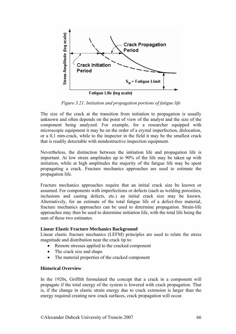
Figure 3.21. Initiation and propagation portions of fatigue life The size of the crack at the transition from initiation to propagation is usually unknown and often depends on the point of view of the analyst and the size of the component being analyzed. For example, for a researcher equipped with microscopic equipment it may be on the order of a crystal imperfection, dislocation, or a 0,1 mm-crack, while to the inspector in the field it may be the smallest crack that is readily detectable with nondestructive inspection equipment. Nevertheless, the distinction between the initiation life and propagation life is important. At low strain amplitudes up to 90% of the life may be taken up with initiation, while at high amplitudes the majority of the fatigue life may be spent propagating a crack. Fracture mechanics approaches are used to estimate the propagation life. Fracture mechanics approaches require that an initial crack size be known or assumed. For components with imperfections or defects (such as welding porosities, inclusions and casting defects, etc.) an initial crack size may be known. Alternatively, for an estimate of the total fatigue life of a defect-free material, fracture mechanics approaches can be used to determine propagation. Strain-life approaches may then be used to determine initiation life, with the total life being the sum of these two estimates. Linear Elastic Fracture Mechanics Background Linear elastic fracture mechanics (LEFM) principles are used to relate the stress magnitude and distribution near the crack tip to:

• Remote stresses applied to the cracked component • The crack size and shape • The material properties of the cracked component

Historical Overview In the 1920s, Griffith formulated the concept that a crack in a component will propagate if the total energy of the system is lowered with crack propagation. That is, if the change in elastic strain energy due to crack extension is larger than the energy required creating new crack surfaces, crack propagation will occur.


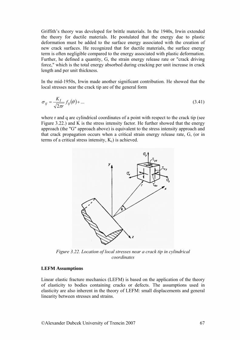
Griffith’s theory was developed for brittle materials. In the 1940s, Irwin extended the theory for ductile materials. He postulated that the energy due to plastic deformation must be added to the surface energy associated with the creation of new crack surfaces. He recognized that for ductile materials, the surface energy term is often negligible compared to the energy associated with plastic deformation. Further, he defined a quantity, G, the strain energy release rate or "crack driving force," which is the total energy absorbed during cracking per unit increase in crack length and per unit thickness. In the mid-1950s, Irwin made another significant contribution. He showed that the local stresses near the crack tip are of the general form

( ) ...2

+= θπ

σ ijI

ij fr

K (3.41)

where r and q are cylindrical coordinates of a point with respect to the crack tip (see Figure 3.22.) and K is the stress intensity factor. He further showed that the energy approach (the "G" approach above) is equivalent to the stress intensity approach and that crack propagation occurs when a critical strain energy release rate, G, (or in terms of a critical stress intensity, Kc) is achieved.

Figure 3.22. Location of local stresses near a crack tip in cylindrical

coordinates LEFM Assumptions Linear elastic fracture mechanics (LEFM) is based on the application of the theory of elasticity to bodies containing cracks or defects. The assumptions used in elasticity are also inherent in the theory of LEFM: small displacements and general linearity between stresses and strains.


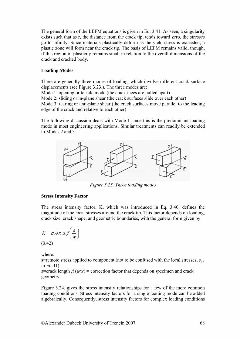
The general form of the LEFM equations is given in Eq. 3.41. As seen, a singularity exists such that as r, the distance from the crack tip, tends toward zero, the stresses go to infinity. Since materials plastically deform as the yield stress is exceeded, a plastic zone will form near the crack tip. The basis of LEFM remains valid, though, if this region of plasticity remains small in relation to the overall dimensions of the crack and cracked body. Loading Modes There are generally three modes of loading, which involve different crack surface displacements (see Figure 3.23.). The three modes are: Mode 1: opening or tensile mode (the crack faces are pulled apart) Mode 2: sliding or in-plane shear (the crack surfaces slide over each other) Mode 3: tearing or anti-plane shear (the crack surfaces move parallel to the leading edge of the crack and relative to each other) The following discussion deals with Mode 1 since this is the predominant loading mode in most engineering applications. Similar treatments can readily be extended to Modes 2 and 3.

Figure 3.23. Three loading modes

Stress Intensity Factor The stress intensity factor, K, which was introduced in Eq. 3.40, defines the magnitude of the local stresses around the crack tip. This factor depends on loading, crack size, crack shape, and geometric boundaries, with the general form given by

⎟⎠⎞

⎜⎝⎛=

wafaK ... πσ

(3.42)

where: s=remote stress applied to component (not to be confused with the local stresses, sij, in Eq.41) a=crack length ,f (a/w) = correction factor that depends on specimen and crack geometry Figure 3.24. gives the stress intensity relationships for a few of the more common loading conditions. Stress intensity factors for a single loading mode can be added algebraically. Consequently, stress intensity factors for complex loading conditions


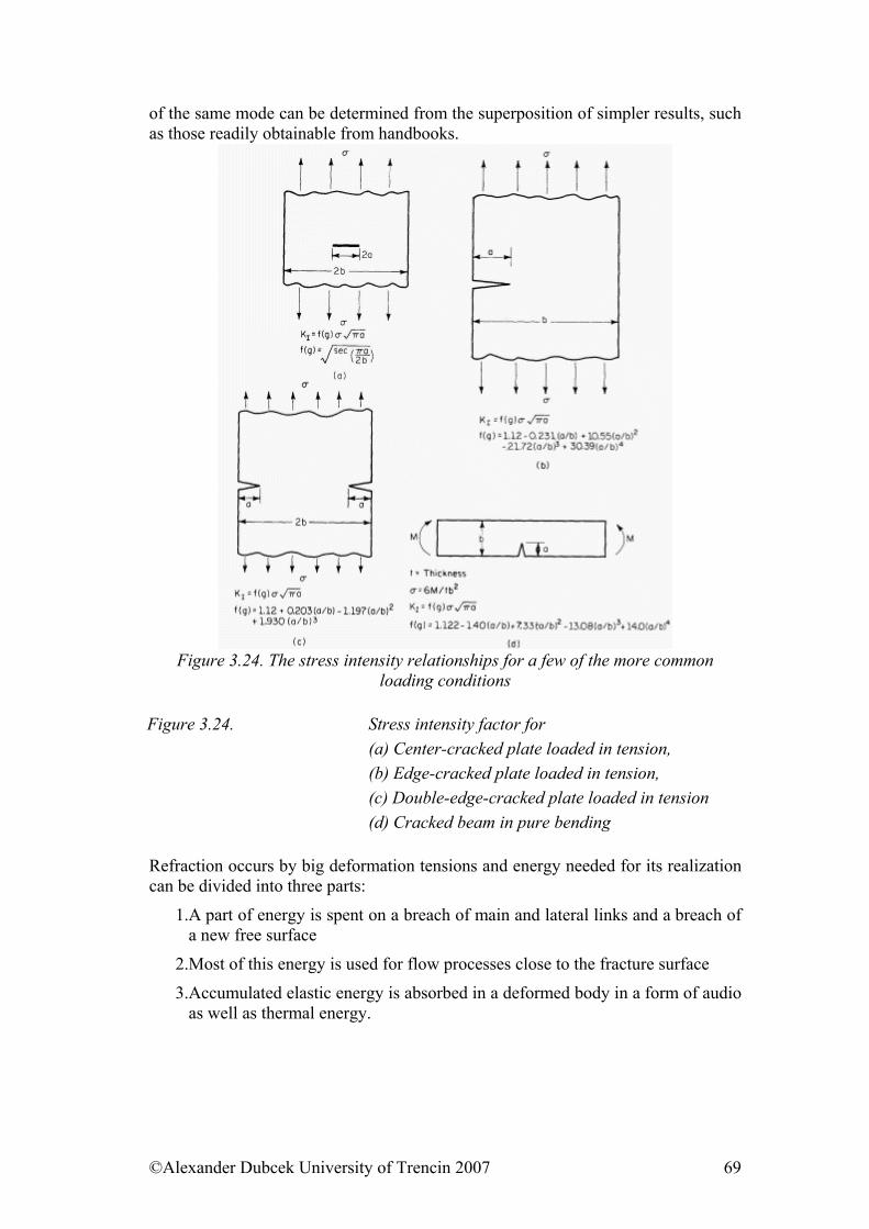
of the same mode can be determined from the superposition of simpler results, such as those readily obtainable from handbooks.

Figure 3.24. The stress intensity relationships for a few of the more common

loading conditions

Figure 3.24. Stress intensity factor for (a) Center-cracked plate loaded in tension, (b) Edge-cracked plate loaded in tension, (c) Double-edge-cracked plate loaded in tension (d) Cracked beam in pure bending Refraction occurs by big deformation tensions and energy needed for its realization can be divided into three parts:

1.A part of energy is spent on a breach of main and lateral links and a breach of a new free surface

2.Most of this energy is used for flow processes close to the fracture surface

3.Accumulated elastic energy is absorbed in a deformed body in a form of audio as well as thermal energy.


We can characterize the fracture action with following processes: a. The existence of submicroscopical flaws and indents b. The creation of the maximum of the tension together with a fully elastic deformation. These maxima arise on ends of microscopical flaws in indents with small radiuses, on inhomogenities, eventually on the surface. c. The creation of molecular skips in the strained area which enables a decrease of critical tensions and a scrubbing of microscopical flaws. d. The creation of a new surface during which not only molecules are split, but also the lateral links. e. Inertial weight nearby the strained place inhibits the spreading of big tensions to longer distances. f. Transformation of a part of elastic energy on the location of the fracture into elastic waves spreading with the speed of sound that support the spread of the fracture g. Creation of ductile (also deformation) fracture in amorphous areas and fragile fracture in crystalline areas. We distinguish slides in the direction of sliding tensions from indents that are abeam toward the direction of acting tension. In the first case the flow occurs nearby the fracture surface where it is possible to watch the creation of characteristic formations that are typical for the ductile fracture. In the case of the fragile fracture no flow occurs. The speed of deformation and the possibility of closing up of molecular indents are characteristic for the kind of the fracture. We talk about so called pulse ductility with regards to fracture tests. The pulse ductility is defined as work needed for breaking through a testing body calculated on the surface unit. If the elastic tension is inhibited to be created in the large area of material with creating of indents during the measurement of the pulse ductility and if high accumulation of tension arises in an indent, then we talk about impact ductility. The hardness of material depends also on a temperature and the length of a testing. Long-term testing gives lower values of the material hardness. Fatigue fractures are given out by repetitive testing. We can attain enhancement of the material hardness for instance by filling, lengthening, adding softeners, and as a result of these, the temperature of vitrification slides to lower temperatures. If we tried to quantify tension relations during a fracture testing on an example of a bearer with the height h, width c, module E and radius of curvature r, we would get for maximal tension with breaking of 1/a2 molecules on the surface unit (it refers to quasi – cubic structure with middle intermolecular distance a) the value of the maximal tension , which is about a centuple higher value than the measured one (calculated for energy C-C link equal to 4.8 10

26max cm/N10.3≈σ

-19J and for interatomic distance a = 0,2 10-9m) This difference can be explained with the fact that not all molecules are strained at the same time. The most strained ones are those whose axis is in the direction of the action of the tension. This re-orientation of molecules into the direction of the acting tension cause extensive hardening of the material. With given tension, this process is in progress in dependency on temperature with delay. The relaxing period ν=τ ∆ 2/e kTU

ii decreases quickly with

increasing temperature, which enables quicker closing up of indents. The tensions therefore vary from a molecule to a molecule with maxima on places of indents.


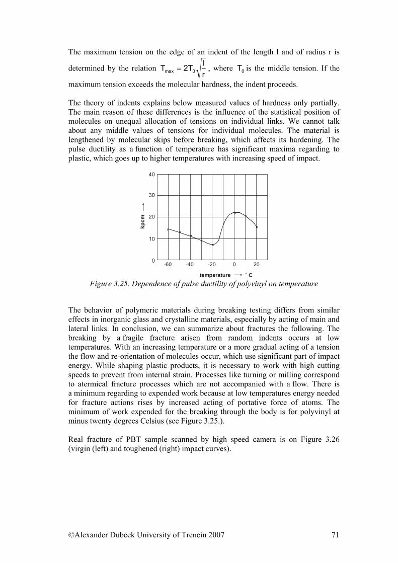
The maximum tension on the edge of an indent of the length l and of radius r is

determined by the relation rlT2T 0max = , where is the middle tension. If the

maximum tension exceeds the molecular hardness, the indent proceeds.

0T

The theory of indents explains below measured values of hardness only partially. The main reason of these differences is the influence of the statistical position of molecules on unequal allocation of tensions on individual links. We cannot talk about any middle values of tensions for individual molecules. The material is lengthened by molecular skips before breaking, which affects its hardening. The pulse ductility as a function of temperature has significant maxima regarding to plastic, which goes up to higher temperatures with increasing speed of impact.

30

40

20

10

0-60 -40 -20 0 20

temperature Co

kpcm

Figure 3.25. Dependence of pulse ductility of polyvinyl on temperature

The behavior of polymeric materials during breaking testing differs from similar effects in inorganic glass and crystalline materials, especially by acting of main and lateral links. In conclusion, we can summarize about fractures the following. The breaking by a fragile fracture arisen from random indents occurs at low temperatures. With an increasing temperature or a more gradual acting of a tension the flow and re-orientation of molecules occur, which use significant part of impact energy. While shaping plastic products, it is necessary to work with high cutting speeds to prevent from internal strain. Processes like turning or milling correspond to atermical fracture processes which are not accompanied with a flow. There is a minimum regarding to expended work because at low temperatures energy needed for fracture actions rises by increased acting of portative force of atoms. The minimum of work expended for the breaking through the body is for polyvinyl at minus twenty degrees Celsius (see Figure 3.25.). Real fracture of PBT sample scanned by high speed camera is on Figure 3.26 (virgin (left) and toughened (right) impact curves).


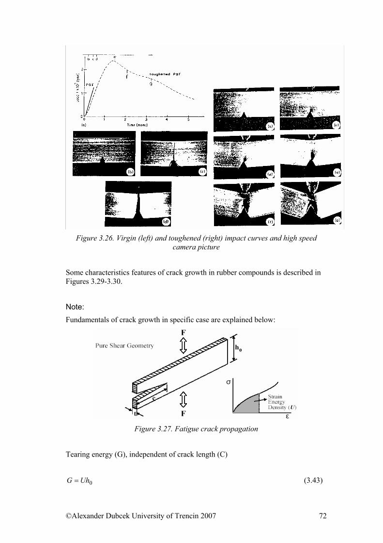
Figure 3.26. Virgin (left) and toughened (right) impact curves and high speed

camera picture

Some characteristics features of crack growth in rubber compounds is described in Figures 3.29-3.30.

Note: Fundamentals of crack growth in specific case are explained below:

Figure 3.27. Fatigue crack propagation

Tearing energy (G), independent of crack length (C)

0UhG = (3.43)


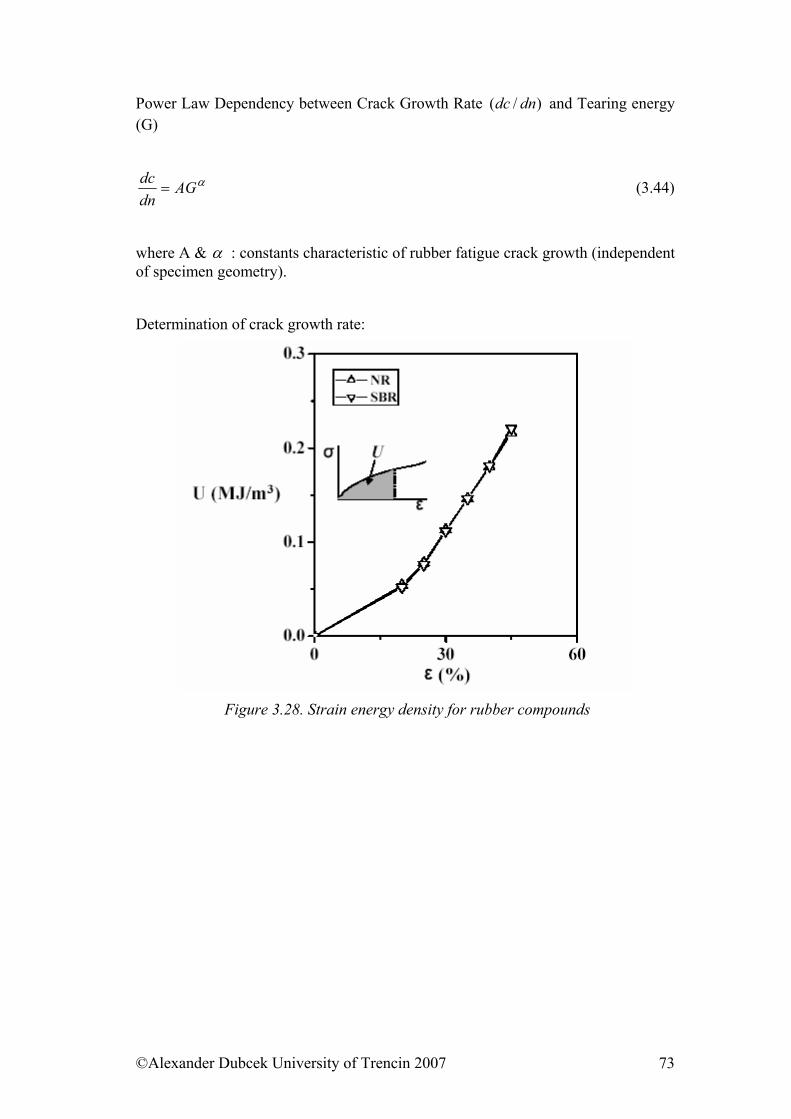
Power Law Dependency between Crack Growth Rate and Tearing energy (G)

)/( dndc

αAGdndc

= (3.44)

where A & α : constants characteristic of rubber fatigue crack growth (independent of specimen geometry).

Determination of crack growth rate:

Figure 3.28. Strain energy density for rubber compounds


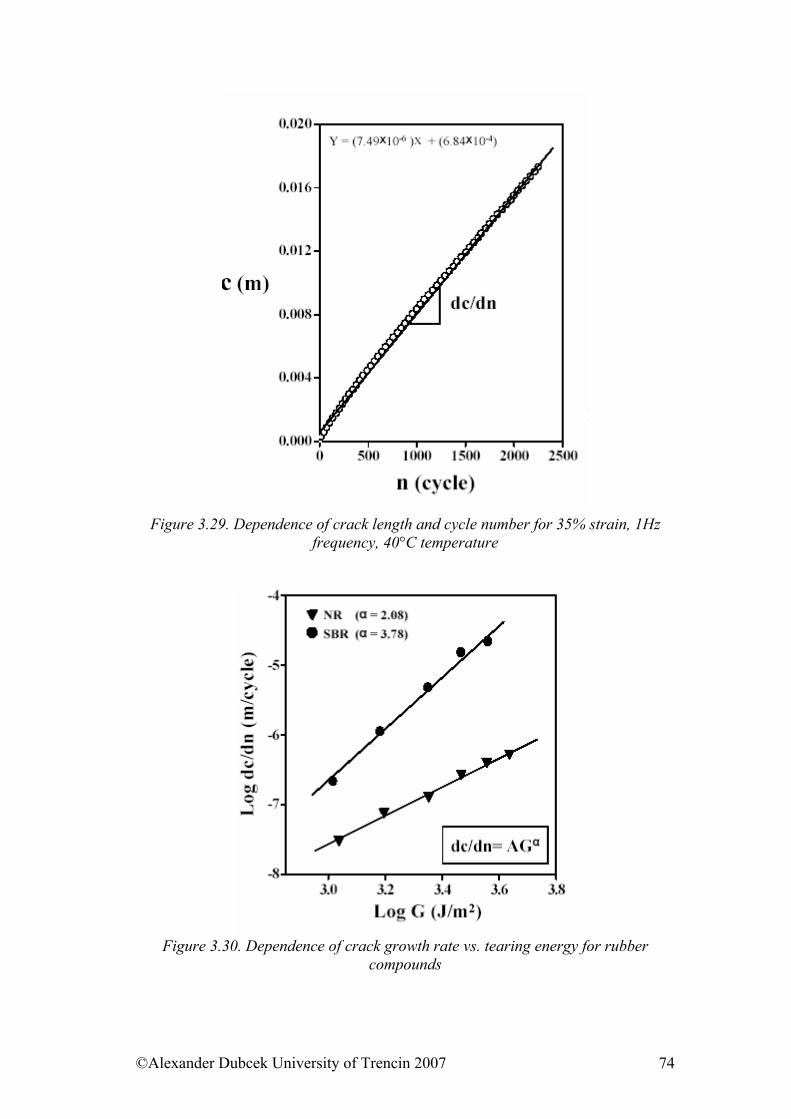
Figure 3.29. Dependence of crack length and cycle number for 35% strain, 1Hz

frequency, 40°C temperature

Figure 3.30. Dependence of crack growth rate vs. tearing energy for rubber

compounds


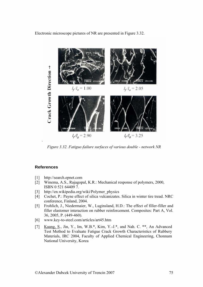
Electronic microscope pictures of NR are presented in Figure 3.32.

.

Figure 3.32. Fatigue-failure surfaces of various double - network NR

References [1] http://search.epnet.com [2] Winema, A.S., Rajagopal, K.R.: Mechanical response of polymers, 2000,

ISBN 0 521 64409 7. [3] http://en.wikipedia.org/wiki/Polymer_physics [4] Cochet, P.: Payne effect of silica vulcanizates. Silica in winter tire tread. NRC

conference, Finland, 2004. [5] Frohlich, J., Niedermaier, W., Luginsland, H.D.: The effect of filler-filler and

filler elastomer interaction on rubber reinforcement. Composites: Part A, Vol. 36, 2005, P. (449-460).

[6] www.key-to-steel.com/articles/art45.htm

[7] Kaang, S., Jin, Y., Im, W.B.*, Kim, Y.-J.*, and Nah. C. **, An Advanced Test Method to Evaluate Fatigue Crack Growth Characteristics of Rubbery Materials, IRC 2004, Faculty of Applied Chemical Engineering, Chonnam National University, Korea


Fundamental questions from presented part 1. What type of forces work at interpretation of viscous properties of

materials? 2. Describe the elastic, viscous and relaxation deformity. 3. What is the definition of tan δ and what its consequence? What identify

the components of complex Young’s modulus? 4. What is the temperature dependence of viscosity? 5. How does the elastic modulus of vulcanizate change in relation to

loading? 6. Explain the reason of Payne effect. What is the task of fillers in Payne

effect? 7. What are the basic models for fracture mechanics? 8. What is characteristic for fracture mechanics of polymers? 9. Name processes, which characterize the fracture action. 10. How does the behavior of polymeric materials during breaking testing

differ from similar effects in inorganic glass and crystalline materials, especially by acting of main and lateral links?


CHAPTER 4 Models of viscoelastic behavior of materials

Objectives to achieve

In this section are introduced basic theoretical approaches describing viscoelastic behavior of materials. Readers will be familiared with basic models: Maxwell, Voigt and their combinations. Now let begin to look into the problem of viscous environments phenomenologically. The Hook’s principle in the symbolic form S⋅= Eσ , whereσ is stress, is strain, E is Young’s modulus, as we already know, is given for an elastic environment. We can write the Newton’s principle of the viscous flowing in the form , where stands for the speed of deformation,

S

ST &⋅= η S& η is dynamic viscosity is , T is tension. The real environment, as we have already said, has viscous as well as elastic attributes. Let us assume, that the tension consists of “the elastic tension” σ and “the viscous tension” T

vT

SESTTv&ησ +=+= . (4.1)

This equation is also called the Kelvin’s equation. If we affect such an environment in time t = 0 with a rectangular impulse of the mechanic tension T0, the deformation of the environment S will be described with the following relation

( )E

eETS t ηττ =−= − ;1 /0 . (4.2)

Consequently, in sufficiently long time the constant deformation ETS 0=∞

independent from the time is formed and the environment is behaving as unviscous. The response of the environment to the applied tension is not obviously immediate, but it gradually reaches the maximum value. The term 4 creep has been employed to describe this process. Likewise after interrupting of the performance of the tension, the deformation decreases exponentially to zero, whereas the relation

determines the relaxation time Eη

=τ . We call this kind of deformation the late

residual deformation. We will introduce the operator of the effective modulus ⟩⟨E for time variable processes of the deformation. For the operator of the effective model it is given

.dtd1E

dtdEE ⎟

⎠⎞

⎜⎝⎛ τ+=η+=⟩⟨ (4.3)


We get by performing of the harmonically changing tension the following:

( ωτ+=ωη+=⟩⟨ i1EiEE ), (4.4) where ω is angular velocity. The above mentioned model of the behavior of viscoelastic substances is called Kelvin’s or also Kelvin – Voigt’s model. Maxwell used different approach to the description of viscoelastic environments, when he assumed that two types of deformations act in an environment, namely elastic and viscous.

ηS+= ESS . (4.5) By deriving the equation 4.5 and by substituting particular values we get equation

ηT

+Eσ

=S'

' . (4.6)

If in time t = 0 the mechanic tension begins to perform in the form of rectangular impulse of the height T0 in the Maxwell’s environment, which stays in the time unchanged, the solution of the equation 4.6 will have the form (see the picture 4.1)

tTETS 00

η+= . (4.7)

The equation 4.7 describes well attributes of many high polymeric materials like colophony, asphalts and others. It is seen from the relation 4.7 that when the tension impulse is short, material is behaving like elastic (the second element in the equation is omissible). The fluxion of the material occurs only at sufficient length of the performing of the tension impulse. Now let in the time t = 0 the rectangular deformation impulse of the height S0 perform, which remains in the time unchanged, in this environment, then the process of the tension dependent on time will be described with the following relation:

EeEST t ηττ == − ;/

0 . (4.8)

We call the process of the exponential decrease of the mechanic tension in dependency on time the relaxation of tension and the particular index τ is called the relaxation time


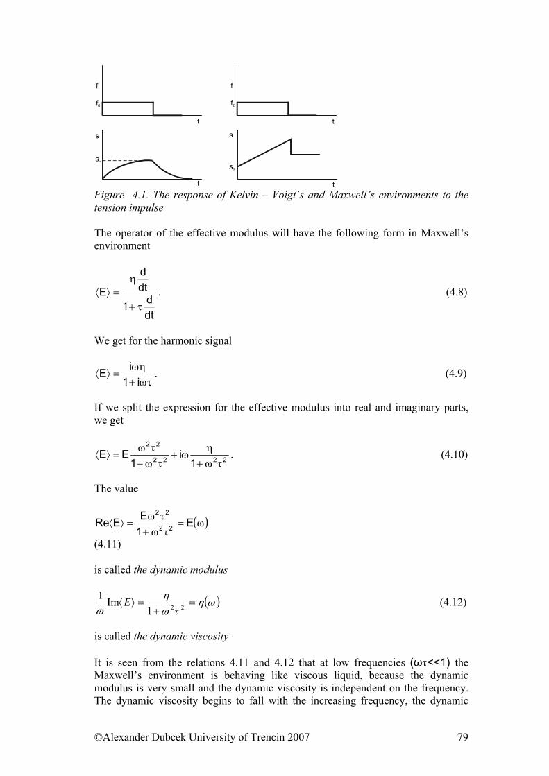
s0

s

f0

t

f

t

f0

t

f

s∞

s

t Figure 4.1. The response of Kelvin – Voigt´s and Maxwell’s environments to the tension impulse The operator of the effective modulus will have the following form in Maxwell’s environment

dtd1

dtd

Eτ+

η=⟩⟨ . (4.8)

We get for the harmonic signal

ωτ+ωη

=⟩⟨i1

iE . (4.9)

If we split the expression for the effective modulus into real and imaginary parts, we get

2222

22

1i

1EE

τω+η

ω+τω+

τω=⟩⟨ . (4.10)

The value

( )ωτωτω E

1EERe 22

22

=+

=⟩⟨

(4.11) is called the dynamic modulus

( )ωητω

ηω

=+

=⟩⟨ 221Im1 E (4.12)

is called the dynamic viscosity It is seen from the relations 4.11 and 4.12 that at low frequencies (ωτ<<1) the Maxwell’s environment is behaving like viscous liquid, because the dynamic modulus is very small and the dynamic viscosity is independent on the frequency. The dynamic viscosity begins to fall with the increasing frequency, the dynamic


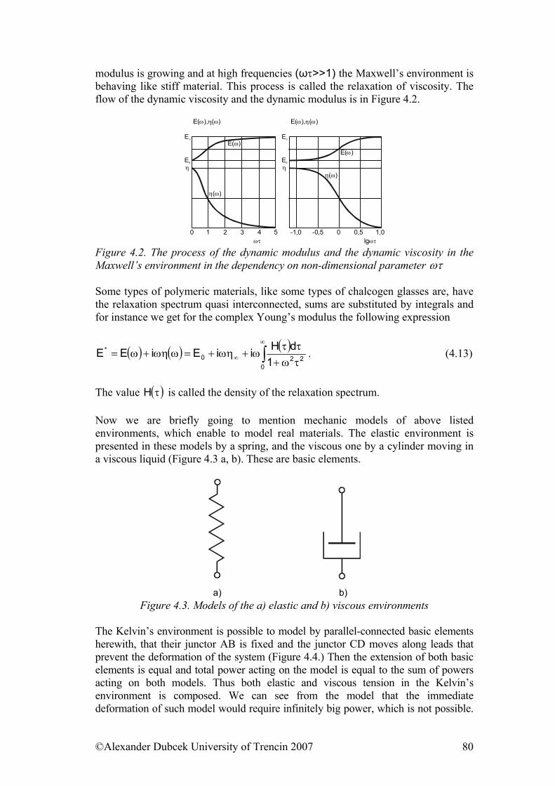
modulus is growing and at high frequencies (ωτ>>1) the Maxwell’s environment is behaving like stiff material. This process is called the relaxation of viscosity. The flow of the dynamic viscosity and the dynamic modulus is in Figure 4.2.

E∞

E0

η

0 54321 -0,5-1,0 0 0,5 1,0

E∞

E0

η

E( )ωE( )ω

η( )ω

η( )ω

E( ),ω η ω( ) E( ),ω η ω( )

lgωτωτ Figure 4.2. The process of the dynamic modulus and the dynamic viscosity in the Maxwell’s environment in the dependency on non-dimensional parameter ωτ Some types of polymeric materials, like some types of chalcogen glasses are, have the relaxation spectrum quasi interconnected, sums are substituted by integrals and for instance we get for the complex Young’s modulus the following expression

( ) ( ) ( )∫∞

∞ τω+ττ

ω+ωη+=ωωη+ω=0

220*

1dHiiEiEE . (4.13)

The value is called the density of the relaxation spectrum. ( )τH Now we are briefly going to mention mechanic models of above listed environments, which enable to model real materials. The elastic environment is presented in these models by a spring, and the viscous one by a cylinder moving in a viscous liquid (Figure 4.3 a, b). These are basic elements.

a) b) Figure 4.3. Models of the a) elastic and b) viscous environments

The Kelvin’s environment is possible to model by parallel-connected basic elements herewith, that their junctor AB is fixed and the junctor CD moves along leads that prevent the deformation of the system (Figure 4.4.) Then the extension of both basic elements is equal and total power acting on the model is equal to the sum of powers acting on both models. Thus both elastic and viscous tension in the Kelvin’s environment is composed. We can see from the model that the immediate deformation of such model would require infinitely big power, which is not possible.


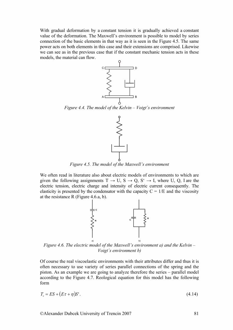
With gradual deformation by a constant tension it is gradually achieved a constant value of the deformation. The Maxwell’s environment is possible to model by series connection of the basic elements in that way as it is seen in the Figure 4.5. The same power acts on both elements in this case and their extensions are comprised. Likewise we can see as in the previous case that if the constant mechanic tension acts in these models, the material can flow.

B

C

A

D

Figure 4.4. The model of the Kelvin – Voigt´s environment

Figure 4.5. The model of the Maxwell’s environment

We often read in literature also about electric models of environments to which are given the following assignments T → U, S → Q, S‘ → I, where U, Q, I are the electric tension, electric charge and intensity of electric current consequently. The elasticity is presented by the condensator with the capacity C = 1/E and the viscosity at the resistance R (Figure 4.6.a, b).

R

C

R C

a) b) Figure 4.6. The electric model of the Maxwell’s environment a) and the Kelvin –

Voigt´s environment b) Of course the real viscoelastic environments with their attributes differ and thus it is often necessary to use variety of series parallel connections of the spring and the piston. As an example we are going to analyze therefore the series – parallel model according to the Figure 4.7. Reological equation for this model has the following form

( 'SEESTv )ητ ++= . (4.14)


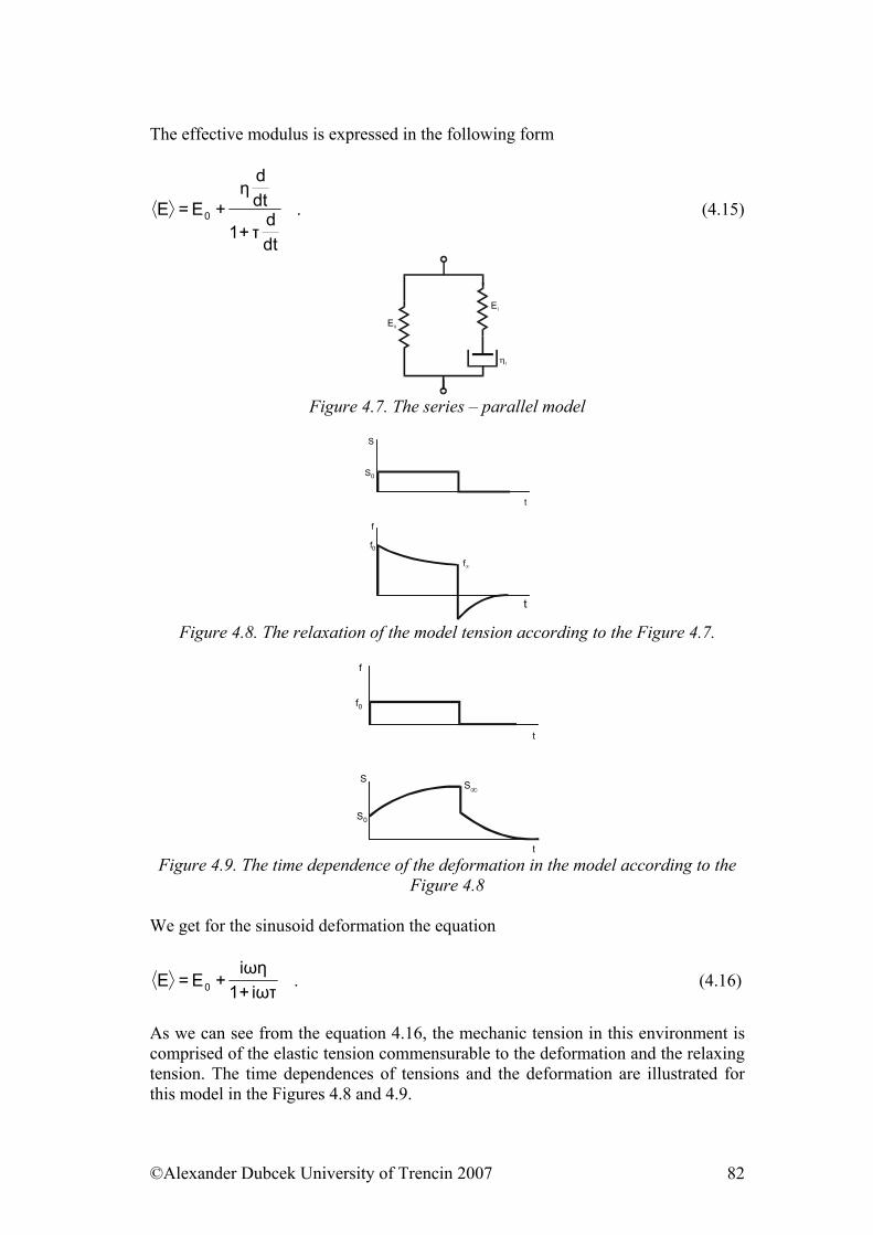
The effective modulus is expressed in the following form

dtd

τ+1

dtd

η+E=E 0 . (4.15)

E0

E1

η1

Figure 4.7. The series – parallel model

t

t

S0

S

f0

f

f∞

Figure 4.8. The relaxation of the model tension according to the Figure 4.7.

t

f0

f

S0

SS∞

t Figure 4.9. The time dependence of the deformation in the model according to the

Figure 4.8 We get for the sinusoid deformation the equation

ωτi+1ωηi

+E=E 0 . (4.16)

As we can see from the equation 4.16, the mechanic tension in this environment is comprised of the elastic tension commensurable to the deformation and the relaxing tension. The time dependences of tensions and the deformation are illustrated for this model in the Figures 4.8 and 4.9.


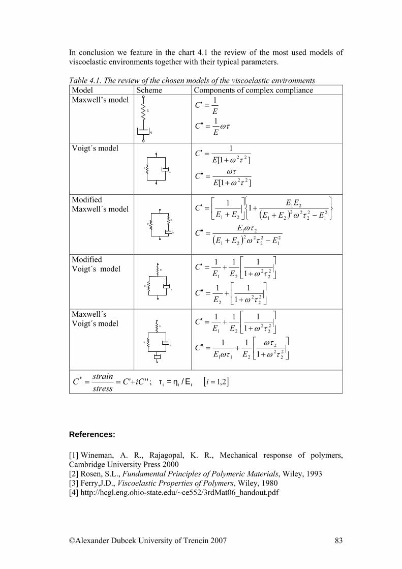
In conclusion we feature in the chart 4.1 the review of the most used models of viscoelastic environments together with their typical parameters. Table 4.1. The review of the chosen models of the viscoelastic environments Model Scheme Components of complex compliance Maxwell’s model

E

η

EC 1

=′

ωτE

C 1=′′

Voigt´s model

E

η

]1[1

22τω+=′

EC

]1[ 22τωωτ+

=′′E

C

Modified Maxwell´s model

E1

E2

η0

( ) ⎭⎬⎫

⎩⎨⎧

−++⎥

⎦

⎤⎢⎣

⎡+

=′2

122

2221

21

21

11EEE

EEEE

Cτω

( ) 21

22

2221

21

EEEE

C−+

=′′τω

ωτ

Modified Voigt´s model

η

E1

E2

⎥⎦

⎤⎢⎣

⎡+

+=′22

221 1

111τωEE

C

⎥⎦

⎤⎢⎣

⎡+

+=′′22

22 1

11τωE

C

Maxwell´s Voigt´s model

η

E1

E2

⎥⎦

⎤⎢⎣

⎡+

+=′22

221 1

111τωEE

C

⎥⎦

⎤⎢⎣

⎡+

+=′′22

22

211 111

τωωτ

ωτ EEC

'''* iCCstressstrainC +== iii E/η=τ; [ ]2,1=i

References: [1] Wineman, A. R., Rajagopal, K. R., Mechanical response of polymers, Cambridge University Press 2000 [2] Rosen, S.L., Fundamental Principles of Polymeric Materials, Wiley, 1993 [3] Ferry,J.D., Viscoelastic Properties of Polymers, Wiley, 1980 [4] http://hcgl.eng.ohio-state.edu/~ce552/3rdMat06_handout.pdf


Fundamental questions from present part:

1. Describe basic physical assumptions of Maxwell model. 2. Describe basic physical assumptions of Voigt model. 3. Explain the map line of the dynamic modulus and dynamic viscosity in

dependency of frequency.


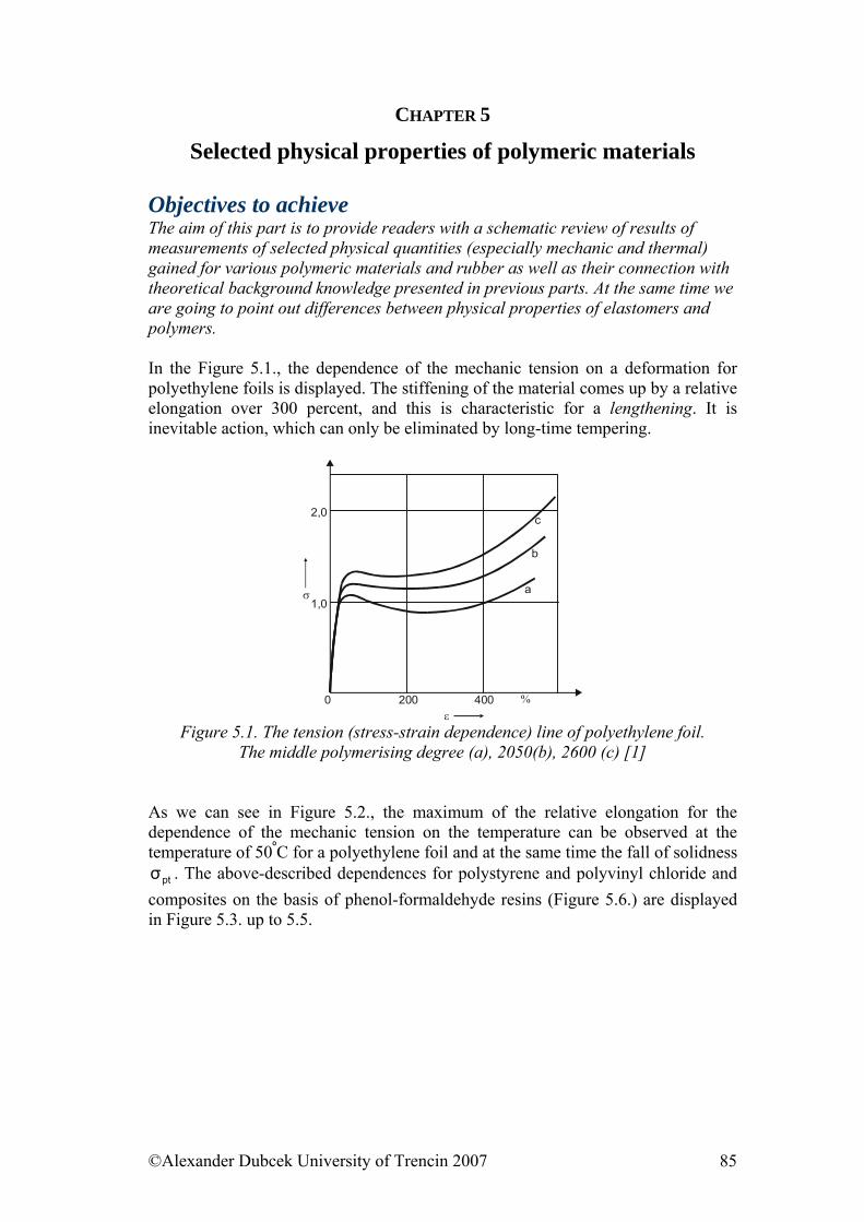
CHAPTER 5

Selected physical properties of polymeric materials Objectives to achieve The aim of this part is to provide readers with a schematic review of results of measurements of selected physical quantities (especially mechanic and thermal) gained for various polymeric materials and rubber as well as their connection with theoretical background knowledge presented in previous parts. At the same time we are going to point out differences between physical properties of elastomers and polymers. In the Figure 5.1., the dependence of the mechanic tension on a deformation for polyethylene foils is displayed. The stiffening of the material comes up by a relative elongation over 300 percent, and this is characteristic for a lengthening. It is inevitable action, which can only be eliminated by long-time tempering.

2,0

1,0

0 200 400 %ε

σ a

b

c

Figure 5.1. The tension (stress-strain dependence) line of polyethylene foil.

The middle polymerising degree (a), 2050(b), 2600 (c) [1] As we can see in Figure 5.2., the maximum of the relative elongation for the dependence of the mechanic tension on the temperature can be observed at the temperature of 50ºC for a polyethylene foil and at the same time the fall of solidness

. The above-described dependences for polystyrene and polyvinyl chloride and composites on the basis of phenol-formaldehyde resins (Figure 5.6.) are displayed in Figure 5.3. up to 5.5.

ptσ


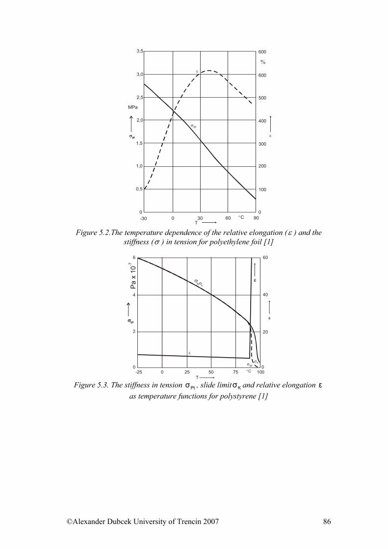
0,5

1,0

1,5

2,0

2,5

3,0

3,5

600

500

400

300

100

00-30 300 60 90

T°C

σpt

σpt

σpt ε

ε

200

600

%

MPa

Figure 5.2.The temperature dependence of the relative elongation (ε ) and the

stiffness (σ ) in tension for polyethylene foil [1]

60

4

2

00 25-25 50 75 100°C

0

6

40

20

σpt

ε

σpt

σpt

σΚ

σΚ

σpt

εε

εε

T

Pa x

10-7

Figure 5.3. The stiffness in tension , slide limit and relative elongation

as temperature functions for polystyrene [1] Ptσ Kσ ε


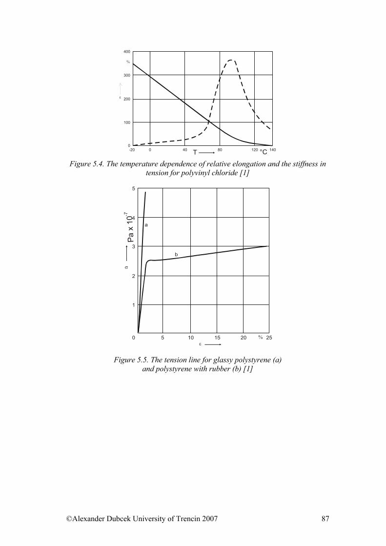
T

ε

%

400

300

200

100

0-20 0 40 80 120 140°C

Figure 5.4. The temperature dependence of relative elongation and the stiffness in tension for polyvinyl chloride [1]

3

4

5

a

b

2

1

0 5 10 15 20 25%ε

σ

Pa x

10-7

Figure 5.5. The tension line for glassy polystyrene (a) and polystyrene with rubber (b) [1]


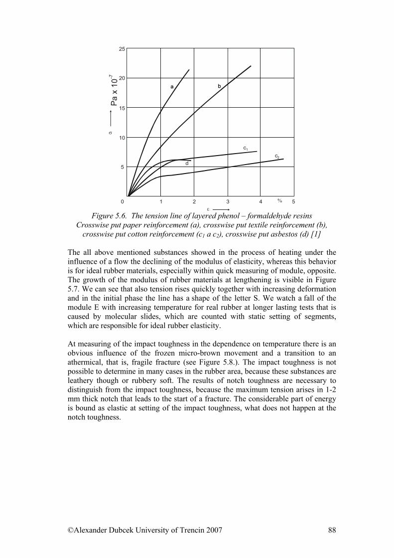
σ

ε

aa b

d

c1

c2

b

0 1 2 3 4 5%

5

10

15

20

25

Pa x

10-7

Figure 5.6. The tension line of layered phenol – formaldehyde resins

Crosswise put paper reinforcement (a), crosswise put textile reinforcement (b), crosswise put cotton reinforcement (c1 a c2), crosswise put asbestos (d) [1]

The all above mentioned substances showed in the process of heating under the influence of a flow the declining of the modulus of elasticity, whereas this behavior is for ideal rubber materials, especially within quick measuring of module, opposite. The growth of the modulus of rubber materials at lengthening is visible in Figure 5.7. We can see that also tension rises quickly together with increasing deformation and in the initial phase the line has a shape of the letter S. We watch a fall of the module E with increasing temperature for real rubber at longer lasting tests that is caused by molecular slides, which are counted with static setting of segments, which are responsible for ideal rubber elasticity. At measuring of the impact toughness in the dependence on temperature there is an obvious influence of the frozen micro-brown movement and a transition to an athermical, that is, fragile fracture (see Figure 5.8.). The impact toughness is not possible to determine in many cases in the rubber area, because these substances are leathery though or rubbery soft. The results of notch toughness are necessary to distinguish from the impact toughness, because the maximum tension arises in 1-2 mm thick notch that leads to the start of a fracture. The considerable part of energy is bound as elastic at setting of the impact toughness, what does not happen at the notch toughness.


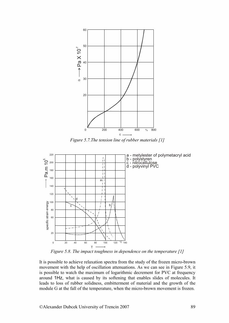
ε

σ

60

50

40

30

20

0 200 400 600 800%

Figure 5.7.The tension line of rubber materials [1]

a

bc

d

T

200

180

160

140

120

100

80

60

20

0 20 40 60 80 100 120 140°C

a - metylester of polymetacryl acid

c - nitrocelluloseb - polystyren

d - polyvinyl PVC

220

Pa.m

105

spec

ific

stra

in e

nerg

y

Figure 5.8. The impact toughness in dependence on the temperature [1]

It is possible to achieve relaxation spectra from the study of the frozen micro-brown movement with the help of oscillation attenuations. As we can see in Figure 5.9, it is possible to watch the maximum of logarithmic decrement for PVC at frequency around 1Hz, what is caused by its softening that enables slides of molecules. It leads to loss of rubber solidness, embitterment of material and the growth of the module G at the fall of the temperature, when the micro-brown movement is frozen.


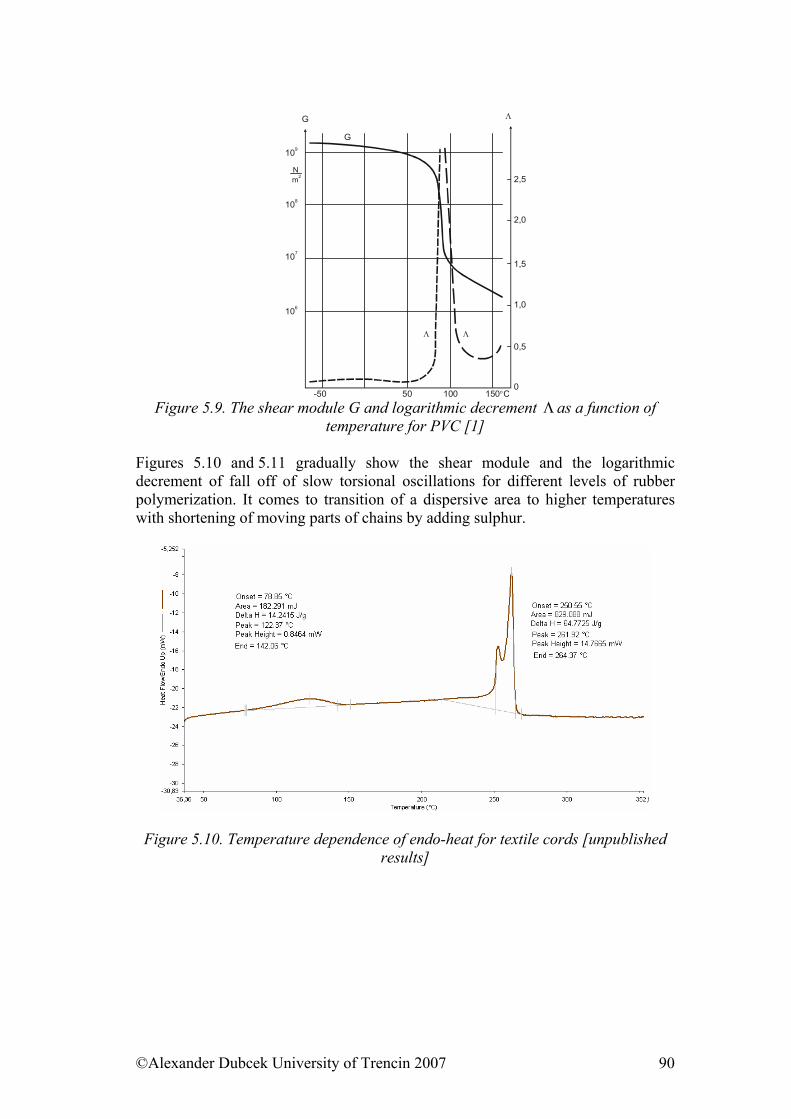
106

107

108

109

-50 50 100 150°C0

0,5

1,5

2,0

2,5

1,0

m2N

G

Λ

ΛΛ

G

Figure 5.9. The shear module G and logarithmic decrement Λ as a function of

temperature for PVC [1] Figures 5.10 and 5.11 gradually show the shear module and the logarithmic decrement of fall off of slow torsional oscillations for different levels of rubber polymerization. It comes to transition of a dispersive area to higher temperatures with shortening of moving parts of chains by adding sulphur.

Figure 5.10. Temperature dependence of endo-heat for textile cords [unpublished results]


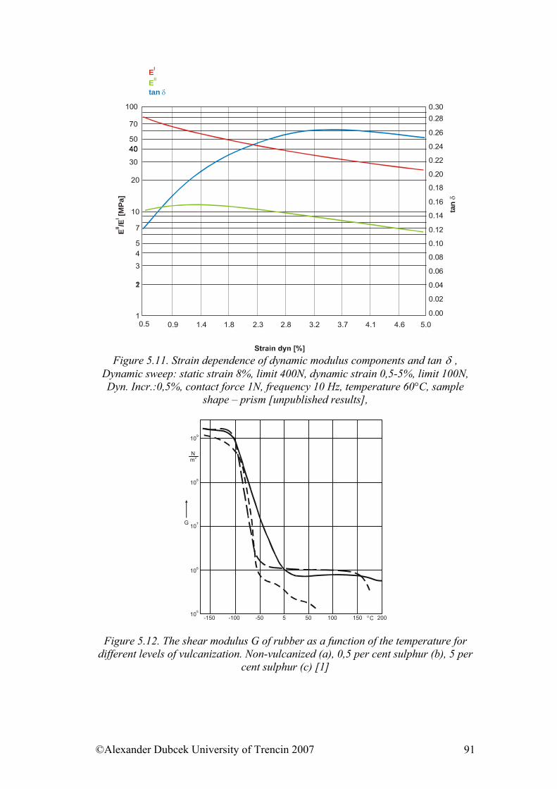
1

12

3

45

7

10

20

30

40404050

70

100 0.300.28

0.26

0.24

0.22

0.20

0.18

0.16

0.14

0.12

0.10

0.08

0.06

0.04

0.02

0.000.5 0.9 1.4 1.8 2.3 2.8 3.2 3.7 4.1 4.6 5.0

EII /EI [M

Pa]

tan

δ

EI

EII

tan δ

Figure 5.11. Strain dependence of dynamic modulus components and tan δ ,

Dynamic sweep: static strain 8%, limit 400N, dynamic strain 0,5-5%, limit 100N, Dyn. Incr.:0,5%, contact force 1N, frequency 10 Hz, temperature 60°C, sample

shape – prism [unpublished results],

108

107

106

105

-150 -100 -50 505 100 150 200°C

109

m2N

G

Figure 5.12. The shear modulus G of rubber as a function of the temperature for different levels of vulcanization. Non-vulcanized (a), 0,5 per cent sulphur (b), 5 per

cent sulphur (c) [1]


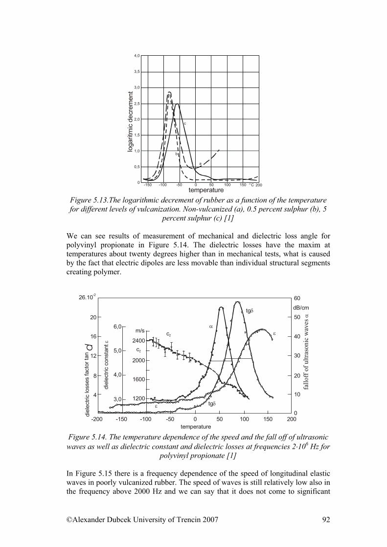
-150 -100 -50 500 100 150 200°C

4,0

3,5

3,0

2,5

2,0

1,5

1,0

0

0,5

c

b

a

temperature

loga

ri tm

ic d

e cre

me n

t

Figure 5.13.The logarithmic decrement of rubber as a function of the temperature for different levels of vulcanization. Non-vulcanized (a), 0.5 percent sulphur (b), 5

percent sulphur (c) [1] We can see results of measurement of mechanical and dielectric loss angle for polyvinyl propionate in Figure 5.14. The dielectric losses have the maxim at temperatures about twenty degrees higher than in mechanical tests, what is caused by the fact that electric dipoles are less movable than individual structural segments creating polymer.

60

50

40

30

20

10

0

dB/cmfa

f of u

ltras

onic

wav

es

llof

α

m/s

2400

2000

1600

1200

6,0

5,0

4,0

3,0

cZ

α

cZ

ε

ε

tgδ

tgδ

diel

ectri

c co

nsta

nt ε

20

16

12

8

4

26.10-2

temperature-200 -150 -100 -50 0 50 100 150 200

diel

ectri

c lo

sses

fact

or ta

n d

Figure 5.14. The temperature dependence of the speed and the fall off of ultrasonic waves as well as dielectric constant and dielectric losses at frequencies 2⋅106 Hz for

polyvinyl propionate [1] In Figure 5.15 there is a frequency dependence of the speed of longitudinal elastic waves in poorly vulcanized rubber. The speed of waves is still relatively low also in the frequency above 2000 Hz and we can say that it does not come to significant


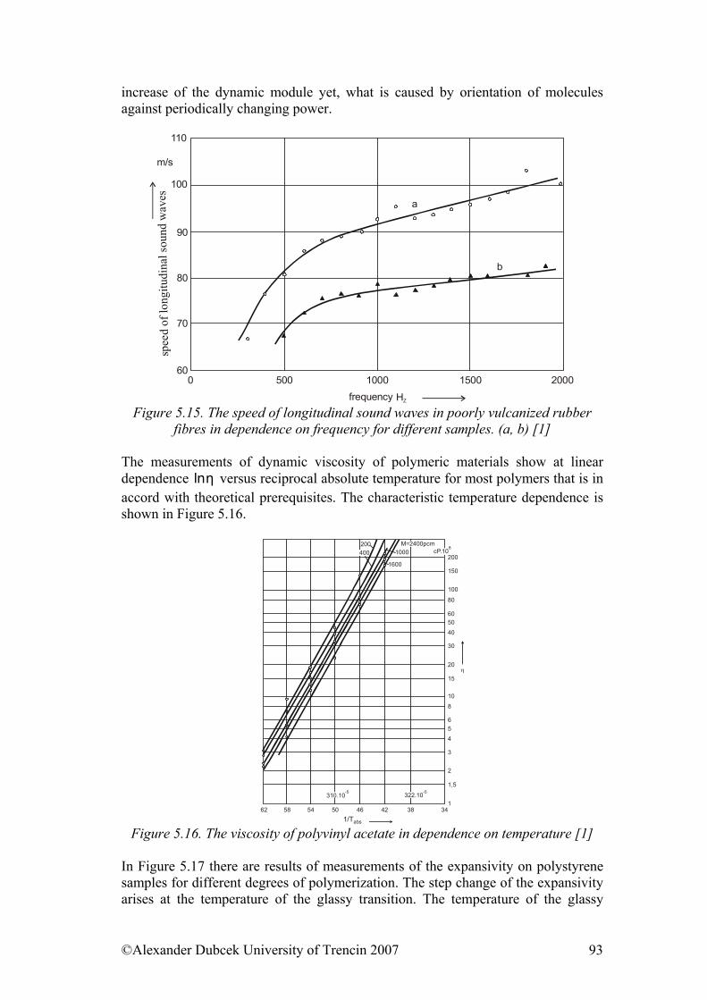
increase of the dynamic module yet, what is caused by orientation of molecules against periodically changing power.

110

100

90

80

70

600 500 1000 1500 2000

HZ

b

a

m/ssp

eed

of lo

ngitu

dina

l sou

nd w

aves

frequency Figure 5.15. The speed of longitudinal sound waves in poorly vulcanized rubber

fibres in dependence on frequency for different samples. (a, b) [1] The measurements of dynamic viscosity of polymeric materials show at linear dependence versus reciprocal absolute temperature for most polymers that is in accord with theoretical prerequisites. The characteristic temperature dependence is shown in Figure 5.16.

ηln

200

150

100

80

6050

40

30

20

10

8

654

2

3

1,5

162 58 54 50 46 42 38 34

1/Tabs

η

1000

1600

15

200400

M=2400pcmcP.10

8

310.10-5 322.10-5

Figure 5.16. The viscosity of polyvinyl acetate in dependence on temperature [1]

In Figure 5.17 there are results of measurements of the expansivity on polystyrene samples for different degrees of polymerization. The step change of the expansivity arises at the temperature of the glassy transition. The temperature of the glassy


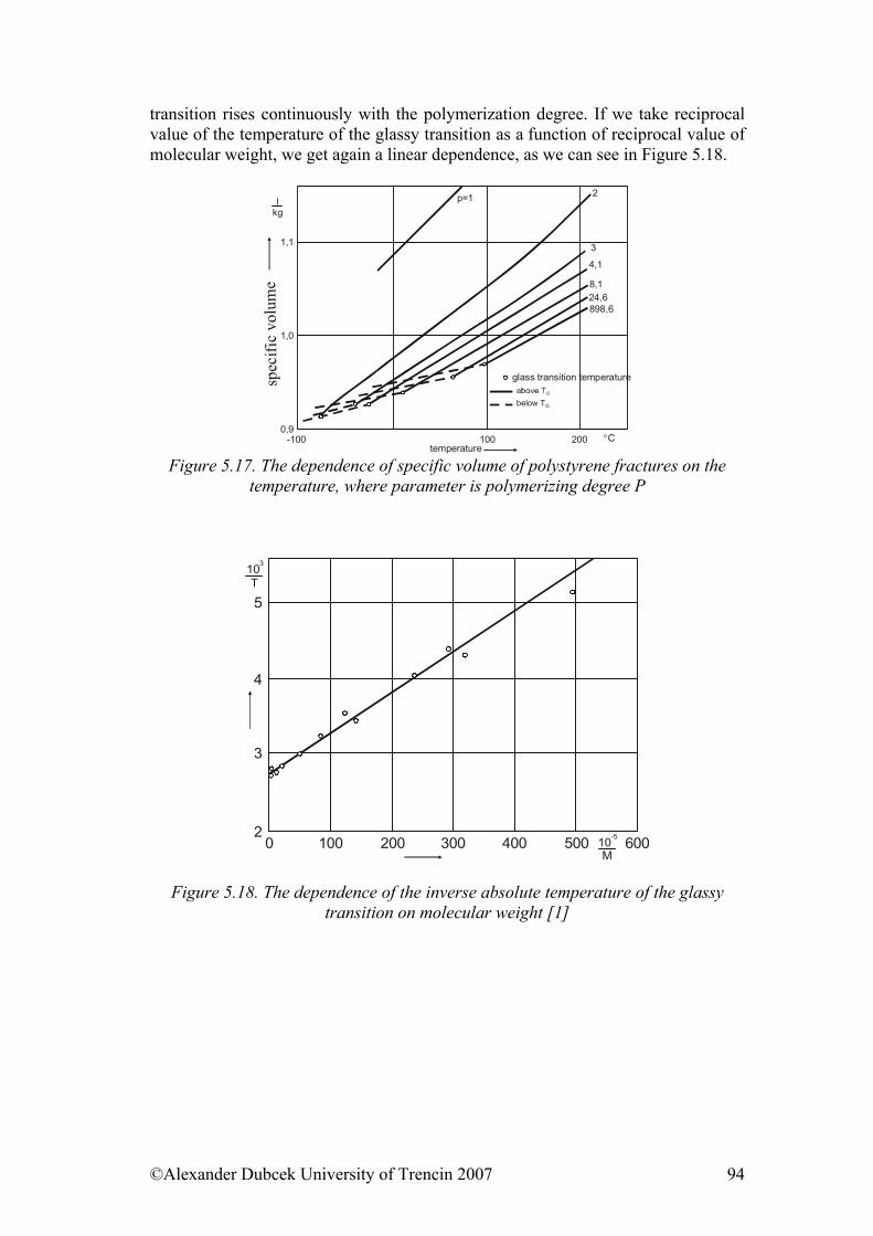
transition rises continuously with the polymerization degree. If we take reciprocal value of the temperature of the glassy transition as a function of reciprocal value of molecular weight, we get again a linear dependence, as we can see in Figure 5.18.

2

3

4,1

8,124,6898,6

below TG

temperature-100 100 200

1,1

1,0

0,9°C

p=1lkg

spec

ific

volu

me

glass transition temperature

Figure 5.17. The dependence of specific volume of polystyrene fractures on the

temperature, where parameter is polymerizing degree P

5

4

3

20 100 200 300 400 500 60010-5

M

103

T

Figure 5.18. The dependence of the inverse absolute temperature of the glassy transition on molecular weight [1]


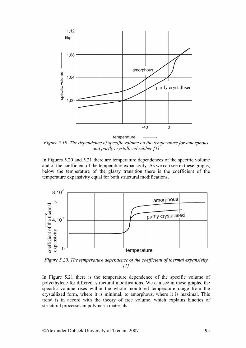
temperature

spec

ific

volu

me

-40 0

1,12

1,08

1,04

1,00

partly crystallised

amorphous

l/kg

Figure 5.19. The dependence of specific volume on the temperature for amorphous

and partly crystallized rubber [1] In Figures 5.20 and 5.21 there are temperature dependences of the specific volume and of the coefficient of the temperature expansivity. As we can see in these graphs, below the temperature of the glassy transition there is the coefficient of the temperature expansivity equal for both structural modifications.

amorphous

0

8.10-4

4.10-4

coef

ficie

nt o

f the

ther

mal

exp

ansi

vity

partly crystallised

1/K

temperature

Figure 5.20. The temperature dependence of the coefficient of thermal expansivity [1]

In Figure 5.21 there is the temperature dependence of the specific volume of polyethylene for different structural modifications. We can see in these graphs, the specific volume rises within the whole monitored temperature range from the crystallized form, where it is minimal, to amorphous, where it is maximal. This trend is in accord with the theory of free volume, which explains kinetics of structural processes in polymeric materials.


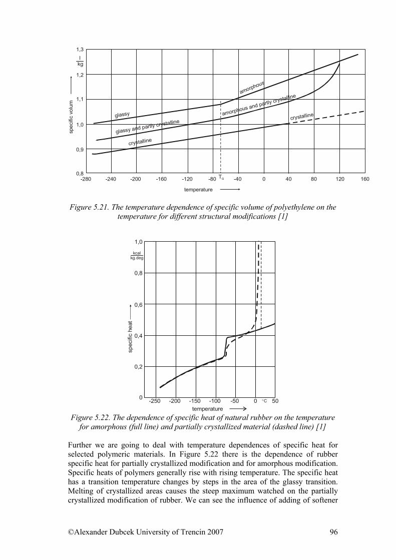
spec

ific

volu

m

1,3

1,2

1,1

1,0

0,9

0,8-280 -240 -200 -160 -120 -80 -40 0 40 80

temperature

lkg

TG

glassy

crystallineglassy and partly crystalline crystallineamorphous and partly crystalline

amorphous

120 160

Figure 5.21. The temperature dependence of specific volume of polyethylene on the

temperature for different structural modifications [1]

1,0

0,8

0,6

0,4

0,2

0 -250 -200 -150 -100 -50 0 50temperature

spec

ific

heat

kcalkg.deg

°C

Figure 5.22. The dependence of specific heat of natural rubber on the temperature

for amorphous (full line) and partially crystallized material (dashed line) [1] Further we are going to deal with temperature dependences of specific heat for selected polymeric materials. In Figure 5.22 there is the dependence of rubber specific heat for partially crystallized modification and for amorphous modification. Specific heats of polymers generally rise with rising temperature. The specific heat has a transition temperature changes by steps in the area of the glassy transition. Melting of crystallized areas causes the steep maximum watched on the partially crystallized modification of rubber. We can see the influence of adding of softener


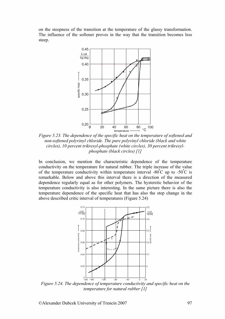
on the steepness of the transition at the temperature of the glassy transformation. The influence of the softener proves in the way that the transition becomes less steep.

00 20 40 60 80 100°C

0,45

0,40

0,35

0,30

0,25

0,20

k.calkg.deg

spec

ific

heat

temperature Figure 5.23. The dependence of the specific heat on the temperature of softened and

non-softened polyvinyl chloride. The pure polyvinyl chloride (black and white circles), 10 percent trikresyl-phosphate (white circles), 30 percent trikresyl-

phosphate (black circles) [1] In conclusion, we mention the characteristic dependence of the temperature conductivity on the temperature for natural rubber. The triple increase of the value of the temperature conductivity within temperature interval -80ºC up to -50ºC is remarkable. Below and above this interval there is a direction of the measured dependence regularly equal as for other polymers. The hysteretic behavior of the temperature conductivity is also interesting. In the same picture there is also the temperature dependence of the specific heat that has also the step change in the above described critic interval of temperatures (Figure 5.24)

0,12

0,10

0,08

0,06

0,04

0,02

0-180 -160 -120 -80 -40 0

0

20

0,1

0,2

0,3

0,4

0,5

k.calkg.deg

k.calm.h.deg

C

λ

tem

pera

ture

con

duct

ivity

spec

ific

heat

Figure 5.24. The dependence of temperature conductivity and specific heat on the

temperature for natural rubber [1]


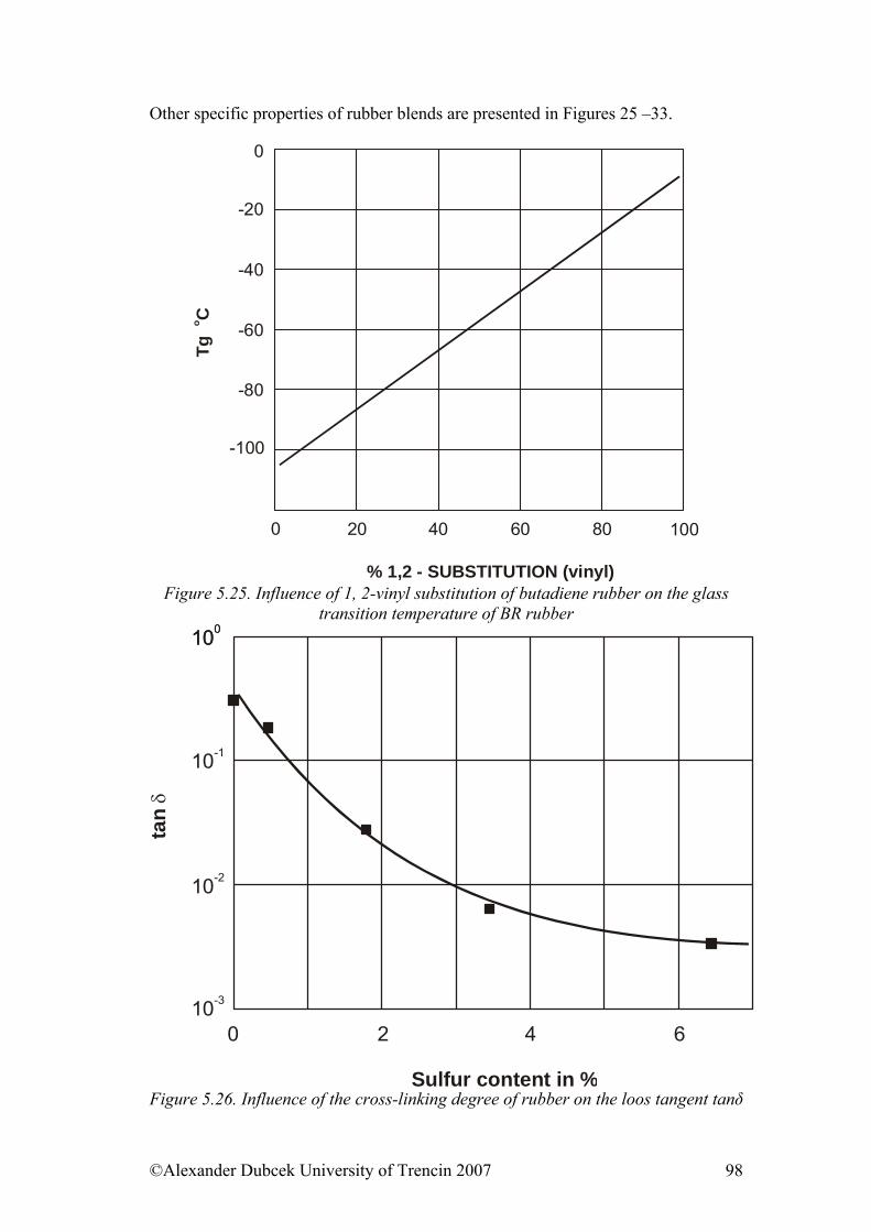
Other specific properties of rubber blends are presented in Figures 25 –33.

20 40 60 80 100

0

-40

-60

-80

-100

-20

0

% 1,2 - SUBSTITUTION (vinyl)

Tg

Co

Figure 5.25. Influence of 1, 2-vinyl substitution of butadiene rubber on the glass

transition temperature of BR rubber

0 2 4 6

100100

10-1

10-2

10-3

tan

δ

Sulfur content in % Figure 5.26. Influence of the cross-linking degree of rubber on the loos tangent tanδ


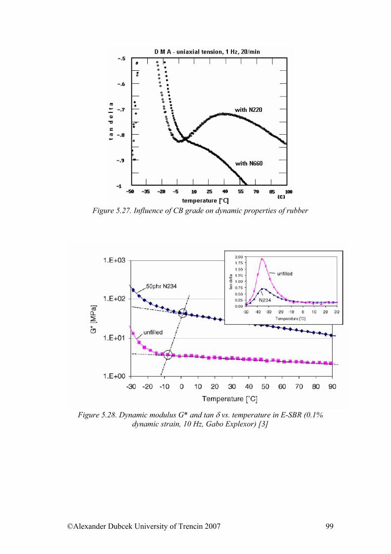
Figure 5.27. Influence of CB grade on dynamic properties of rubber

Figure 5.28. Dynamic modulus G* and tan δ vs. temperature in E-SBR (0.1%

dynamic strain, 10 Hz, Gabo Explexor) [3]


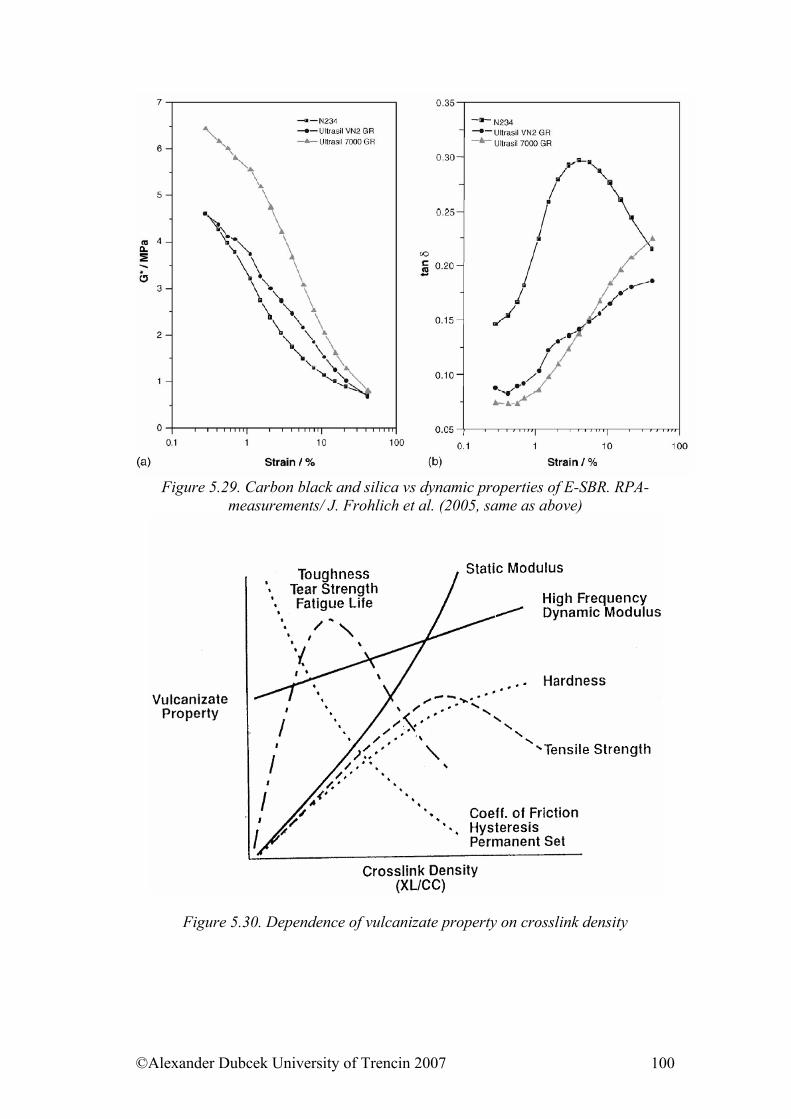
Figure 5.29. Carbon black and silica vs dynamic properties of E-SBR. RPA-

measurements/ J. Frohlich et al. (2005, same as above)

Figure 5.30. Dependence of vulcanizate property on crosslink density


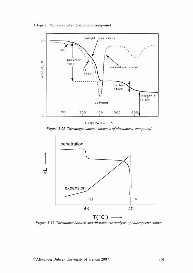
A typical DSC curve of an elastomeric compound

Figure 5.32. Thermogravimetric analysis of elastomeric compound

Tg Ts

expansion

penetration

∆L

T( C )o

-43 -40

Figure 5.33. Thermomechanical and dilatometric analysis of chloroprene rubber


References: [1] Holzmüller, W., Altenburg, K., Physics of Polymer, SNTL Prag 1966, (czech version) [2]M. Schubnell, J. E. K. Schawe, Mettler Toledo GmbH, Sonnenbergstrasse 74, CH-8603 Schwerzenbach, Switzerland [3]J. Frohlich*, W. Niedermeier, H.D. Luginsland, Composites: Part A 36 (2005) 449–460 Fundamental questions from present part: 1. Explain main differences in behaviour of viscoelastic and elastomer materials according to figures from this chapter. 2.Explain main differences of static and dynamic dependences of choosen physical parameters on the base of study material from this chapter. 3. Explain characteristic points form dependence of specific volume vs. Temperature for amorphous and partly crystalline polymer. 4.What is the influence of sulphur content in rubber compounds on tan δ ? 5.Explain the difference in dependence modulus vs. strain for fillers carbon black and silica.


CHAPTER 6

Electrical properties of polymers Objective to achieve Introducing the specific resistivity and conductivity. Dielectric properties of polymers, electrical stress of polymers. Percolation threshold.

6.1. Electrically Conductive Polymers Electrical conductivity of almost all polymers in pure state is very low. It is defined from fundamental relation, which describes the dimension dependence of electrical resistance in the form

slR .ρ

= (6.1)

where ρ is specific resistance, l is conductor length, s is cross-section of conductor. From this relation we can obtain specific resistance in form

lsR.

=ρ (6.2)

In some cases it is more convenient to introduce specific conductivity as an inverse value of specific resistance in the form

[ 11.1 −−Ω= mρ

σ ] (6.3)

Values of specific resistance range from 1010 to 1014 . From this point of view we can regard polymer materials as very good insulants. Certain increase of electrical conductivity is caused mostly by presence of dirt, that is why you have to work in dustless environment e.g. when working on preparation of insulants with extremely high specific resistance. Presence of microheterogeneities in structure offers creation possibility of free charge bound onto its own structure. Such microheterogeneities can be boundary lines between amorphous and crystalline phase, where thermal activation of electric charge can occur. This increase in conductivity has ionic character and occurs as result of present dirt dissociation.

mOhm.

Despite the fact that most polymers are dielectrics with very good insulating properties, there are some inherently conductive polymers, too. Those are mostly macromolecules with system of conjugated bonds in string. When we expose these polymers in strong oxidizer or deoxidizer they become significantly more electrically conductive. Most widely known conductive polymers are primarily trans-polyacetylene, then polypyrrole, polythiophene (and its derivates on the basis of poly-3-alkyltiophenes), polyaniline, poly-p-phenylene and some other. These materials have found important applications, mostly if you need to use conductive


materials in corroding medium, where you cannot use metals. Problem is the fact that conjugated structures are formed by polymer strings with low mobility and therefore polymers with such structure are practically unworkable by common technologies. Forming directly during synthesis (e.g. creation of conductive polymer layer on electrode surface) is needed for their application, or application in the form of colloids or composites, where conductive polymer acts as the filler. In certain circumstances even polymer without conjugated bonds can be highly conductive. E.g. when we affect polyisoprene with iodic vapours we can get increase of his conductivity to as many as 10-1 S/cm. But opinions on charge-transfer mechanism in such systems are still very divergent.

6.2. Electrically Conductive Composites Other possibility how to get electrically conductive materials on the basis of polymers is preparation of electrically conductive composites. The principle is very simple. You have to mix electrically conductive filler into non-conductive thermoplastic die, what will ensure significantly increased conductivity. In contrast to electrically inherently conductive polymers, advantages of these materials lie in the fact that they can be formed with technologies used for thermoplastics, even though the high proportion of filler and high viscosity (that is associated with it) make preparation of composite by mixing of components above melting temperature of polymer die, as well as following thermal forming very difficult. For fillers we can basically use any particles or fibres that are electrically conductive. Most commonly used are various forms of hydrogen, mostly soots (carbon black) and graphite, metal elements (we can use colloid elements of silver to get extreme conductivity on the level of metals), as well as conductive polymers in the form of powder. Elements of conventional polymers coated with layer of metal or conductive polymer are another interesting possibility. These are advantageous, because of their similar density to die, if we want to use the filler in a melt or solution (e.g. for conductive adhesive) and we want to prevent filler sedimentation while stocking. In terms of conductivity we observe an interesting effect at conductive composites and that is existence of so-called percolation threshold. It is manifested by intense increase of conductivity by few orders in narrow interval of conductive filler concentration. Explanation of this phenomenon lies in conception of creation of conductive connections through whole geometrical section of observed body. Conductivity is proportionally increased along with gradual increase of conductive filler concentration, as shown in Figure 1, what is caused by quick skip of electrons over bordered areas in material that are formed by clusters of conductive filler. Number of these agglomerates and their size is gradually increasing along with growth of filler concentration, while conductivity is growing more or less linearly within the range of circa 2 – 3 orders.


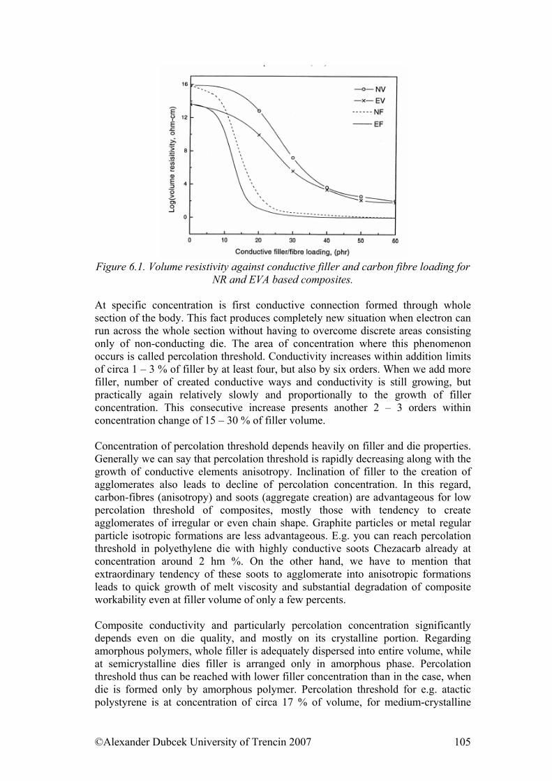
Figure 6.1. Volume resistivity against conductive filler and carbon fibre loading for

NR and EVA based composites. At specific concentration is first conductive connection formed through whole section of the body. This fact produces completely new situation when electron can run across the whole section without having to overcome discrete areas consisting only of non-conducting die. The area of concentration where this phenomenon occurs is called percolation threshold. Conductivity increases within addition limits of circa 1 – 3 % of filler by at least four, but also by six orders. When we add more filler, number of created conductive ways and conductivity is still growing, but practically again relatively slowly and proportionally to the growth of filler concentration. This consecutive increase presents another 2 – 3 orders within concentration change of 15 – 30 % of filler volume. Concentration of percolation threshold depends heavily on filler and die properties. Generally we can say that percolation threshold is rapidly decreasing along with the growth of conductive elements anisotropy. Inclination of filler to the creation of agglomerates also leads to decline of percolation concentration. In this regard, carbon-fibres (anisotropy) and soots (aggregate creation) are advantageous for low percolation threshold of composites, mostly those with tendency to create agglomerates of irregular or even chain shape. Graphite particles or metal regular particle isotropic formations are less advantageous. E.g. you can reach percolation threshold in polyethylene die with highly conductive soots Chezacarb already at concentration around 2 hm %. On the other hand, we have to mention that extraordinary tendency of these soots to agglomerate into anisotropic formations leads to quick growth of melt viscosity and substantial degradation of composite workability even at filler volume of only a few percents. Composite conductivity and particularly percolation concentration significantly depends even on die quality, and mostly on its crystalline portion. Regarding amorphous polymers, whole filler is adequately dispersed into entire volume, while at semicrystalline dies filler is arranged only in amorphous phase. Percolation threshold thus can be reached with lower filler concentration than in the case, when die is formed only by amorphous polymer. Percolation threshold for e.g. atactic polystyrene is at concentration of circa 17 % of volume, for medium-crystalline


low-density polyethylene it is around 8 – 10 %, while for highly crystalline low-density polyethylene it is only circa 5 %. These data are, of course, only for orientation and they significantly depend on filler quality as well. As we have mentioned before, sudden increase of conductivity in the area of percolation threshold is caused by creation of conductive ways that consist of conductive filler over entire section of experimental body. It can be easily understood that during mechanical deformation of conductive composite with rubber die and volume of conductive filler over percolation concentration comes to decline of conductivity, because quite rigid conductive connections can be relatively easily disrupted during uniaxial deformation. On the other hand, consequential return into former state after stress release mostly does not lead to restoration of former conductivity before deformation force application, but proportions are much more complicated. Similar effects of conductivity change can be also observed at the change of conductive composite dimensions in consequence of thermal expansivity at warming or cooling of the material. Another important feature of these materials is substantial embrittlement at filler volume increase. It can be characterized e.g. by value of elongation at abruption. It is interesting that area of concentration, where steepest decline of elongation occurs, corresponds to percolation area with substantial increase of conductivity. The explanation is based on reasoning, that creation of conductive ways from filler elements presents also facilitated way for the growth of mechanic fissure at the application of deformation force. Fissure is thus created at lower stress and its growth is much quicker, if only there is a connection structure of body through whole volume.

6.3. Influence of Force Field on Polymer Behaviour Under the term force field we will in this chapter understand mostly the influence of electric, eventually magnetic field. From this point of view we can define two types of substances and that is Electric current conductor that allows irreversible transport of electrically charged elements of particle character. Dielectric or insulator, where electric dislocation emerges that is caused by creation of induced dipoles, or by orientation of dipoles yet present in material, while this dislocation is accompanied by energy accumulation and is reversible after field disposal. Transition between these two groups of substances is fluent and external conditions such as temperature are also influencing the properties. Divisions according to the electric conductivity value σ is approximately as follows: metals with conductivity of 102 to 106 S/m (Siemens per meter), semiconductors, which have conductivity within the interval of 10-8 to 102 S/m and insulators with lower conductivity than 10-

8 S/m, while common insulators reach values of 10-12 to 10-15 with the limit somewhere around 10-30 S/m. From practical point of view is group of antistatic substances an important one. It has sufficient surface conductance for dispersion of


electrostatic charge that is created e.g. at friction. Conductivity of these substances is in the sphere of less conductive semiconductors, i.e. around 10-6 S/m. Change of conductivity along with temperature is also worthy of note. Metal conductivity is decreasing along with growing temperature, while conductivity for substances from next two groups is with temperature growing. For the growth of conductivity with temperature we can use Arrhenius type formula σ = σ∞ exp (-Ea / RT), (6.4) where σ∞ is anteexponential factor with conductivity function at very high temperature and Ea is activation energy of conductivity. However equation 10.1 suits for polymers only in narrow range of temperatures.

6.4. Electrical Strength of Polymers As we have mentioned before, substantial quality of dielectric is its insulating power, i.e. the ability to resist electric field influence. But this quality depends on external conditions; in this case it is mostly intensity of influencing electric field. Absolute intensity is reached at gradual increase of field intensity and dielectric conductivity will arise to values that are characteristic for conductors. This state is from outside manifested by dielectric breakdown. Electric voltage, corresponding to field intensity is called breakdown voltage Up. When it is applied to thickness, it characterizes electric strength Ep = Up / d, where Ep has parameters of electric field, i.e. V /m. Breakdown mechanism is difficult and sometimes it does not depend on thickness and time. Most commonly you get relative datum Ep by direct measuring and this datum depends on sample geometry and measuring conditions. Electric strength cannot be for this reason considered as material characteristics and we have to use standardized experiments for its determination. Electric strength of polymers depends besides external conditions (temperature, body geometry) on polymer structure. Generally we can say that electric strength is growing along with decrease of string elements mobility and along with the growth of molecule cohesion. From this point of view it decreases in following order: e.g. polyvinyl-alcohol > polymethyl-methacrylate > polystyrene. It is lowest for non-polar polymers with high mobility of segments, e.g. polyolefins and rubber. On the basis of what has been said before, the observed decrease of Ep in the area above temperature of glassy transition where mobility of strings differs substantially appears to be logical. Ep grows with the grade of arrangement as well, e.g. crystallinity. From the molecular point of view we can stress out the indirect proportion to free volume.


6.5. Dielectric Properties of Polymers Polymers are typical dielectrics with low electric conductivity and relatively high electric strength. Every dielectric is outwardly electrically neutral, because it contains equal number of positive and negative charges in dipoles. However dipole orientation in the direction of influencing field occurs in electric field, it is so-called polarization of dielectric. If we connect voltage supply U to the plate condenser, it will be practically at once charged with charge +Q or –Q, while the quantity of charge Qo = Co U is directly proportional to the electric voltage U and constant of proportionality Co with the size of Farad, F = C x V-1, is called vacuum capacity of condenser. Surface density of electric charge is thus directly proportional to the field intensity between plates E = U / d. If we fill the space between plates by dielectric, polarization occurs by the action of electric field. Capability rate of dielectric to polarize itself is quantity called electric polarization P that is given by formula

EDP 0ε−= (6.5) where D is electric induction (D = εE, while ε presents dielectric permittivity) and εo is vacuum permittivity. These quantities are dielectric’s capability rate to polarize itself, to increase condenser capacity and to decrease force effect of electric field. Generally, dielectric polarization is function of time. This quantity consists of more components that differ in time reaction on the field change. Electric polarization Pe occurs on the level of particular atoms and is caused by transition of external electrons from electric shell. Dipoles in time interval of 10-15 s order are created in this way. Atomic polarization runs slower, in time 10-13 s, and it is created by influence of electric field on polar bond, whereby mutual distance of atoms in bond and bond angle are changed. Electronic and atomic polarization present so-called deformational polarization Pd. This can be considered as prompt at frequency of field polarity change lower than 1012 and origin of such induced dipoles will be in phase with changing electric field. The most important of these polarizations is so-called elastic dipole polarization that is caused by elastic dipole deflection in electric field from their equilibrium positions with lowest energy, which dipoles occupy in the environment of adjacent molecules out of field influence. These three polarization types are included in the common term of elastic polarization and it is characterized by quick, practically immediate adoption of particular state after electric field application and practically immediate return into its former state after the field is disrupted. But there are permanent dipoles in many substances, too, that are formed by polar bonds between two atoms with different electroaffinity. Bonding electrons e.g. in the carbon – chlorine bond are attracted more to chlorine atom with heavier positively charged nucleus. Generally this bond is permanent dipole with partial positive charge on carbon. In contrast to elastic dipole polarization we assume that permanent dipole can also have more equilibrium positions that are qualitatively


different. Change of these positions is conditioned by overcoming of potential barrier. If such a permanent dipole gets into electric field, it will try to orientate itself in the field direction and so-called orientation polarization Po occurs. But this action is slowed down in consequence of interaction with adjacent groups and thus it is time-dependent. Overall time flow can be at most substances, including polymers, described by three-parameter function P(t) = Pd + Po(1 – e-t / τ), (6.6) where Po is limiting value of orientation polarization that will occur at t → ∞ and τ is so-called relaxation time. If condenser is in static electric field with constant intensity, electric induction will be monotonous function of time. But if we change field intensity with certain frequency, then polarization does not follow sudden field changes immediately, but with particular delay. Development of field intensity can be written in the form E(t) = Eamp cos ϖ t . (6.7) Electric induction is also sine function with the same frequency, but delayed by time period that can be expressed by phase angle D(t) = Damp cos (ϖ t - δ). (6.8) For every frequency ϖ are amplitudes in relation Damp = εo ε(ϖ) Eamp, (6.9) where ε(ϖ) is frequency dependent dielectric permittivity. (Permittivity is the criterion of polarizability and equals to surface density of charge / field intensity.) Electric induction can be divided into two vector segments, D(t) = D’ cos ωt + D’’sin ωt, (6.10) one of them is in phase with influencing field and other one is displaced by 90o. While D = εa ε (ω) E, (6.11) we define vector components ε’ and ε’’ that are also frequency dependent and are defined ε’ = ε cos δ and ε’’= ε sin δ. (6.12) First one characterizes real component of permittivity, i.e. its relative capacity and other one represents loss properties of dielectric. Deformation polarization components are determined in time 10-13 - 10-15 s and they manage to adapt to the field change. Relaxation time is higher at orientation


polarization, and that is for low-molecular substances 10-8 up to 10-12 and for polymers even higher. At small frequencies, both polarization components (deformation and orientation) manage to watch field changes, time delay is zero and δ = 0. Orientation component at high frequencies practically cannot respond to field change, ε’ (∞) = ε∞, and losses are zero again, ε” = 0. Between these extreme limits lies area, where values are non-zero and it is possible to measure relaxation areas characteristic for specific material. In contrast to elastic polarization that occurs immediately, in the case of orientation dipole polarization we assume that dipole has more equilibrium positions. It can change these positions after potential energetic barrier overcoming, e.g. thermal energy. If we gradually increase field frequency, then we get from the area, where both components manage to watch changes and we observe maximum and constant induction, into the area where loss element is delayed by constant time period and finally at high frequencies we get back to the area where induction is in phase, because loss element cannot by any chance respond to field change. Frequencies, phase transitions are observed at (viz. demonstration of loss element) are characteristic for specific structure, what means that motions of dipoles liable to orientation polarization are influenced by material structure. If the structure changes e.g. by temperature change, addition of free volume influencing additive, change of strings arrangement (e.g. branching and such), then we also observe changes in position of registered motions on frequency axis, as well as in the level of response characterizing intensity of particular motions. In this way we can register relaxation spectrum, interpretation of which is qualitatively equal to the spectrum acquired by DMTA method, thus it reflects presence of segments with various structure. That is why this spectrum can be used for observed material characterization. We have to say that by this method we will get relaxation spectra that are usually much more complex than spectra acquired by dynamic-mechanical analysis. Thus they offer more information on studied material, but on the other hand their interpretation is more difficult as well. This method is less spread, comparing to DMTA, and that is also because of experiment requirements and advanced technical difficulties on measuring devices.

References [1] Job, A.E., Oliveira, F.A., Alves, N., Giacommetti, J.A., Mattoso, L.H.C.: Conductive composites of natural rubber and carbon black for pressure sensors. Synthetic metals, 135-136 (2003). P.(99-100). [2] Bertetto, A.M, Ruggiu, M.: Low cost resistive based touch sensor. Mechanics Research Communications 30 (2003) P.(101–107). www.elsevier.com/locate/mechrescom [3] N.C. Das, N.C, Khastgir, D., Chaki, T.K., Chakraborty, A.: Electromagnetic interference shielding effectiveness of carbon black and carbon fibre filled EVA and NR based composites. Received 10 September 1999; received in revised form 6 March 2000; accepted 23 March 2000. [4] Sau, K.P., Chaki, T.K., Khastgir, D.: Carbon fibre filled conductive composites based on nitrile rubber (NBR), ethylene propylene diene rubber (EPDM) and their blend. Rubber Technology Centre, Indian Institute of Technology, Kharagpur,


India. (Received 12 May 1997, revised 4 August 1997, accepted 10 September 1997). [5] Volf, J. – Holý, S. – Vlček, J.: Using of Tactile Transducer for Pressure-Distribution Measurement on the Sole of the Foot. In: Sensors and Actuators (A), 1997, No. 62, P. ( 556-561). Fundamental questions from presented part

1. What does cause that conductivity is proportionally increased along with gradual increase of conductive filler concentration?

2. What does the composite conductivity depend and particularly percolation concentration on?

3. What is polarization of dielectric? 4. What we can say in generally about electric strength? 5. What are inherently conductive polymers?


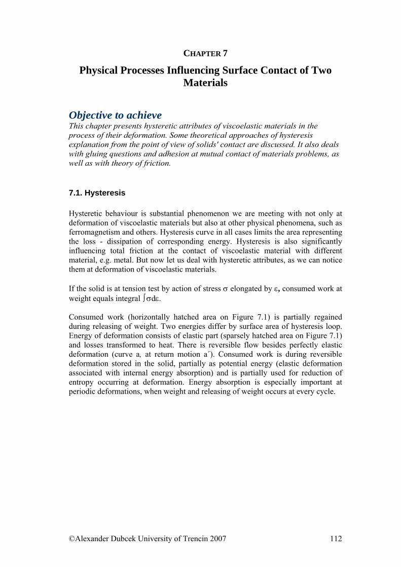
CHAPTER 7

Physical Processes Influencing Surface Contact of Two Materials

Objective to achieve This chapter presents hysteretic attributes of viscoelastic materials in the process of their deformation. Some theoretical approaches of hysteresis explanation from the point of view of solids' contact are discussed. It also deals with gluing questions and adhesion at mutual contact of materials problems, as well as with theory of friction.

7.1. Hysteresis Hysteretic behaviour is substantial phenomenon we are meeting with not only at deformation of viscoelastic materials but also at other physical phenomena, such as ferromagnetism and others. Hysteresis curve in all cases limits the area representing the loss - dissipation of corresponding energy. Hysteresis is also significantly influencing total friction at the contact of viscoelastic material with different material, e.g. metal. But now let us deal with hysteretic attributes, as we can notice them at deformation of viscoelastic materials. If the solid is at tension test by action of stress σ elongated by ε, consumed work at weight equals integral ∫ σdε. Consumed work (horizontally hatched area on Figure 7.1) is partially regained during releasing of weight. Two energies differ by surface area of hysteresis loop. Energy of deformation consists of elastic part (sparsely hatched area on Figure 7.1) and losses transformed to heat. There is reversible flow besides perfectly elastic deformation (curve a, at return motion a´). Consumed work is during reversible deformation stored in the solid, partially as potential energy (elastic deformation associated with internal energy absorption) and is partially used for reduction of entropy occurring at deformation. Energy absorption is especially important at periodic deformations, when weight and releasing of weight occurs at every cycle.


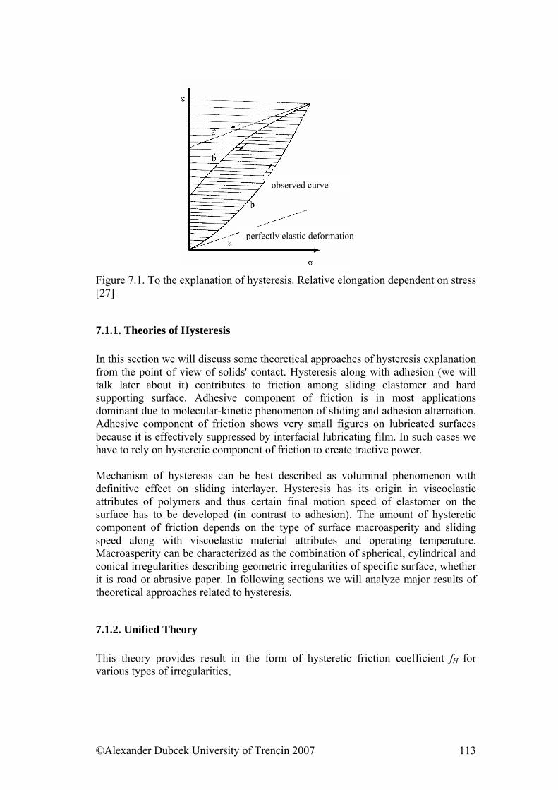
observed curve

perfectly elastic deformation

Figure 7.1. To the explanation of hysteresis. Relative elongation dependent on stress [27]

7.1.1. Theories of Hysteresis In this section we will discuss some theoretical approaches of hysteresis explanation from the point of view of solids' contact. Hysteresis along with adhesion (we will talk later about it) contributes to friction among sliding elastomer and hard supporting surface. Adhesive component of friction is in most applications dominant due to molecular-kinetic phenomenon of sliding and adhesion alternation. Adhesive component of friction shows very small figures on lubricated surfaces because it is effectively suppressed by interfacial lubricating film. In such cases we have to rely on hysteretic component of friction to create tractive power. Mechanism of hysteresis can be best described as voluminal phenomenon with definitive effect on sliding interlayer. Hysteresis has its origin in viscoelastic attributes of polymers and thus certain final motion speed of elastomer on the surface has to be developed (in contrast to adhesion). The amount of hysteretic component of friction depends on the type of surface macroasperity and sliding speed along with viscoelastic material attributes and operating temperature. Macroasperity can be characterized as the combination of spherical, cylindrical and conical irregularities describing geometric irregularities of specific surface, whether it is road or abrasive paper. In following sections we will analyze major results of theoretical approaches related to hysteresis.

7.1.2. Unified Theory This theory provides result in the form of hysteretic friction coefficient fH for various types of irregularities,


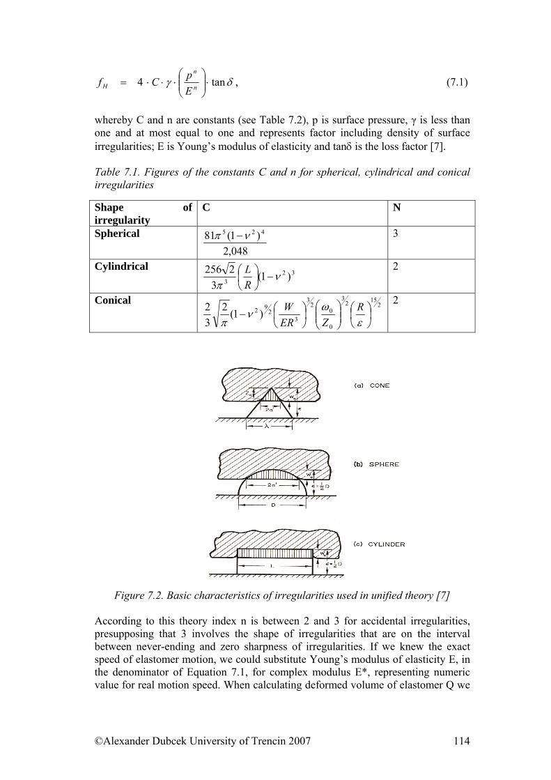
δγ tan4 ⋅⎟⎟⎠

⎞⎜⎜⎝

⎛⋅⋅⋅= n

n

H EpCf , (7.1)

whereby C and n are constants (see Table 7.2), p is surface pressure, γ is less than one and at most equal to one and represents factor including density of surface irregularities; E is Young’s modulus of elasticity and tanδ is the loss factor [7]. Table 7.1. Figures of the constants C and n for spherical, cylindrical and conical irregularities

Shape of irregularity

C N

Spherical 048,2

)1(81 425 νπ − 3

Cylindrical 32

3 )1(3

2256 νπ

−⎟⎠⎞

⎜⎝⎛

RL

2

Conical 2152

3

0

02

3

32

92 )1(232

⎟⎠⎞

⎜⎝⎛

⎟⎟⎠

⎞⎜⎜⎝

⎛⎟⎠⎞

⎜⎝⎛−

εω

νπ

RZER

W 2

Figure 7.2. Basic characteristics of irregularities used in unified theory [7] According to this theory index n is between 2 and 3 for accidental irregularities, presupposing that 3 involves the shape of irregularities that are on the interval between never-ending and zero sharpness of irregularities. If we knew the exact speed of elastomer motion, we could substitute Young’s modulus of elasticity E, in the denominator of Equation 7.1, for complex modulus E*, representing numeric value for real motion speed. When calculating deformed volume of elastomer Q we


neglect contact asymmetry in sliding direction, hence this effect increases the value of adhesive friction coefficient.

7.1.3. Relaxation Theory This theory of hysteresis is based on energy method of analysis and suggests simple Maxwell's model of viscoelastic behaviour. It regards movement of elongated and hard spherical solid upon the surface of elastomeric material. Surface of rigid body is considered as smooth and thermal effects as constant on the surface of contact during sliding. Negligible effect of adhesive friction component is also assumed. Result of these considerations is inferred formula:

δαβξ tan. ⋅⎟

⎠⎞

⎜⎝⎛⋅⎟

⎠⎞

⎜⎝⎛⋅=

EpAf H , (7.2)

where ξ is linear ratio, A is numerical factor contingent on the shape irregularity and ratio β /α characterizes the shape of irregularity (β >1 , α >1). Out of the form of formula 7.2 for fH we can see, that it is analogical to the formula 7.1. Result of this theory is similar equation as the one in previous theory, despite different approach. This analysis seems to be more rigorous than previous one. Also with respect to the index in ratio (p/E), that reaches higher values in unified theory while here it is equal to one. It is remarkable that in every theory of adhesion and hysteresis is friction coefficient proportional to tanδ, adhesive component is dependent on ratio (E/p) and hysteretic component of friction is dependent on its reciprocal. It would be adequate to replace modulus E in previous equations with complex value E* because of the change possibility in speed and sliding temperature.

7.2. Gluing and adhesion Another phenomenon significantly influencing dynamic behaviour of materials at their mutual contact is adhesion. However, this phenomenon has much complex use. Development of varnishes and glues required not only the knowledge about their internal structure but also about the processes causing their adhesion to the surface. It starts to shape up that from coupling forces it is mostly dispersion forces, dipole moments and hydrogen bonds that determine firmness of glued joints. At the same time we have to mention that there are remarkable differences between calculated force values and measured firmness of glued joints that is influenced mostly by following factors: Macroscopic and submicroscopic asperities are practically allowing only partial contact of glue lines. Therefore glue has to have as low surface tension as possible to penetrate within limits into most of cavities and cracks.


Aqueous films, thin layers of grease, dissolvent and softeners have negative impact on adhesion of glued layers. Atmospheric pressure causes increase in firmness of adhesion. If we want to glue large areas, we have to use diluted liquid glues or low-molecular glues to ensure adhesion of glue to the surface. Curing of the glue occurs at the evaporation of dissolvent and polymerization, only rarely at its solidification. If surface of the solid is harsh or porous (leather, wood, plaster), glues must diffuse quickly into the pores of material. Situation is different with glass and metals. Evaporation of dissolvent must happen before pressing of glued materials, but glue areas still have soft consistence. Plastics during gluing are swelling and etching by action of the glue. Volume shrinking occurs during solidification of the glue and also creation of cavities and cracks, eventually creation of irregular surface and big shearing stress decreasing joint firmness. Creation of interfering interlayers often depends on absorption quality of glued surface and glue. Hygroscopic are mostly alkaline glass areas binding water or its vapour that is destroying glued joint. All plastic materials exposed to water for quite a long time will transmit water vapour. Metals also incline to oxidation and creation of hydroxides. Material under the layer of glue or varnish will corrode, bubbles will occur or varnish will tear. Above mentioned facts show that surface tension has important role during realization of quality adhesion. Under the term surface tension σF we understand the stress affecting on unit of length of marginal curve limiting the material. It is identical with the work needed for creation of square unit of the new surface and it can be expressed by following formula

dll=dA F ⋅⋅σ , (7.3) whereby l⋅ dl is areal element, occurred at surface enlargement. During tension test of the solid we have to subtract elastic deformation energy Ap affecting square unit (it will demonstrate in the form of sound and kinetic energy of fragments) that we will express by formula

( )2l

El =A2

P∆ , (7.4)

where ∆ l is deformation to athermal fracture, E is Young's modulus and l is the length of tested solid.


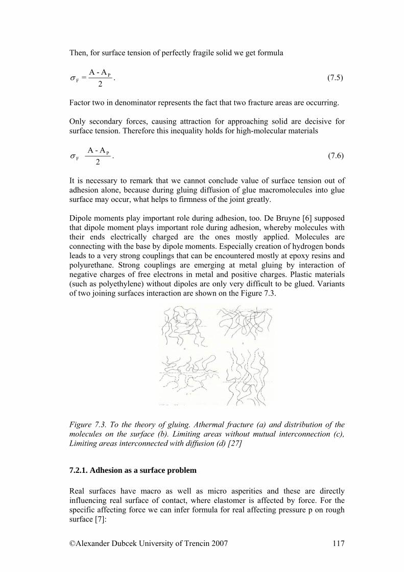
Then, for surface tension of perfectly fragile solid we get formula

2A-A

= PFσ . (7.5)

Factor two in denominator represents the fact that two fracture areas are occurring. Only secondary forces, causing attraction for approaching solid are decisive for surface tension. Therefore this inequality holds for high-molecular materials

2A-A P

Fσ . (7.6)

It is necessary to remark that we cannot conclude value of surface tension out of adhesion alone, because during gluing diffusion of glue macromolecules into glue surface may occur, what helps to firmness of the joint greatly. Dipole moments play important role during adhesion, too. De Bruyne [6] supposed that dipole moment plays important role during adhesion, whereby molecules with their ends electrically charged are the ones mostly applied. Molecules are connecting with the base by dipole moments. Especially creation of hydrogen bonds leads to a very strong couplings that can be encountered mostly at epoxy resins and polyurethane. Strong couplings are emerging at metal gluing by interaction of negative charges of free electrons in metal and positive charges. Plastic materials (such as polyethylene) without dipoles are only very difficult to be glued. Variants of two joining surfaces interaction are shown on the Figure 7.3. Figure 7.3. To the theory of gluing. Athermal fracture (a) and distribution of the molecules on the surface (b). Limiting areas without mutual interconnection (c), Limiting areas interconnected with diffusion (d) [27]

7.2.1. Adhesion as a surface problem Real surfaces have macro as well as micro asperities and these are directly influencing real surface of contact, where elastomer is affected by force. For the specific affecting force we can infer formula for real affecting pressure p on rough surface [7]:


p = (Aapp/Aact) * papp, (7.7) where we can imagine apparent area Aapp as contact area of completely smooth surface and Aact is actual area, that is summation of particular areas of asperity apexes for the real surface. Almost every theory describing adhesion claims, that fA is inversely proportional to the affecting pressure, and thereby the existence of macro irregularities reduces coefficient of adhesion. Generally, contact surface of tyres is needed to have certain pattern in the place of contact with the road to get slip-resistant rate and that is despite illogicality that contact surface will reduce. Solution of this evidently contradictory fact resides, of course, in distribution of adhesion on the wet as well as on the dry road. On the dry road we will get maximal adhesion on the smooth surface of tread without design. But when the road is wet, there is continual film of liquid on the contact surface suppressing adequate adhesion and it is declining to a very low level. That is why common tyres must have tread design. It is very complicated to define exact contact surface between elastomer and accidentally coarsened surface by experimentation. In literature we can find a summary of distribution dependencies of rubber elements on hard and smooth surface. It is documented by data in Table 7.2. In practice, rubber is elastic and generally contact surface A appears to be directly proportional to the expression (p/E´)n. Kragelskij [7] defined: n = (2s/2s+1), (7.8) where s involves characteristic values of rubber elements’ particular shapes and n increases in dependence on distribution complexity of rubber elements. It was ascertained that n is nearing to one for the model with the most complex distribution, but also in that case is hard surface smooth what is far away from real surfaces.


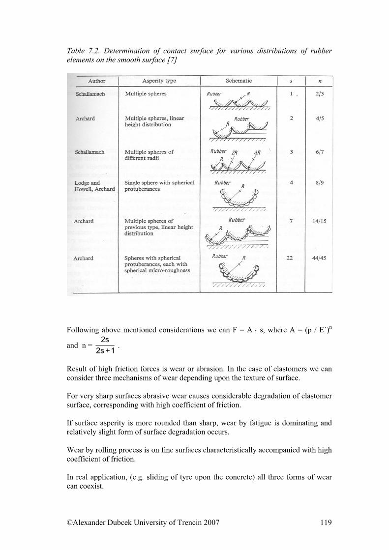
Table 7.2. Determination of contact surface for various distributions of rubber elements on the smooth surface [7]

Following above mentioned considerations we can F = A ⋅ s, where A = (p / E´)n

and n = 1+s2

s2 .

Result of high friction forces is wear or abrasion. In the case of elastomers we can consider three mechanisms of wear depending upon the texture of surface. For very sharp surfaces abrasive wear causes considerable degradation of elastomer surface, corresponding with high coefficient of friction. If surface asperity is more rounded than sharp, wear by fatigue is dominating and relatively slight form of surface degradation occurs. Wear by rolling process is on fine surfaces characteristically accompanied with high coefficient of friction. In real application, (e.g. sliding of tyre upon the concrete) all three forms of wear can coexist.


Perhaps most widely used index of wear is abrasiveness γ that is defined as follows: γ = A / f , (7.9) where A is abrasive factor and f is coefficient of friction at sliding.

7.2.2. The Role of Adhesion at Dynamic Contact of Two Materials – Macroscopic and Molecular Understanding Friction force generated between moving solids consists of adhesion and deformation part. Adhesion part manifests itself on the surface in the areas that are going deeper not more than molecule dimensions, whereas deformation is dimensional phenomenon. Exact nature of adhesion is not clear although it is generally supposed that it consists of creation and interruption of joints on the molecular level. In the case of elastomers we can suppose occurrence of adhesion by two mechanisms, namely macroscopic or molecular mechanism. From macroscopic point of view, for overall adhesive force FADH holds: FADH = ∑ Fi = ∑ Ai . Si, (7.10) where Ai is local macroscopic contact surface between elastomer and hard rough base, Si is local shearing stress in mesophase. On the molecular level, following the theory of Kummer [9], we can write for any place of the joint Fi = ni . ji, (7.11) where ni is number of molecular joints and couplings between elastomer and base in the place i, ji is effective joint force. Equations 7.10 and 7.11 result in formula Si = (ni / Ai) . ji (7.12) and thereby local shear stress of macroscopic model is function of the molecular joint force ji. In the course of last years several theories of elastomer adhesion on smooth and rough surfaces were presented. Some of them were based on molecular-kinetic behaviour of individual molecules. Other theories followed phenomenological theory and are based on mechanical model of spring and absorber.


7.2.3. Ratio Theory This theory is based on principle of various contact times of elastomer with surface. It defines so-called ”variable time τ“; it is time from interruption of the joint and elastomer to recreation of a new one [10]:

⎥⎦

⎤⎢⎣

⎡⋅⋅= Tk

Ea

e0ττ , (7.13) where Ea is activation energy, T is absolute temperature, k is Boltzmann’s constant, τ0 for elastomers has value 10-12 s. Speed of elastomer slide is defined by formula

⎥⎦⎤

⎢⎣⎡

⋅⎥⎦⎤

⎢⎣⎡

⋅ ⋅⎥⎦

⎤⎢⎣

⎡⋅⋅⋅

⋅⋅=⋅= Tk

EaTk

Ea

eTk

FeVV0

1 2 τγλ (7.14)

V1 depends on the friction force F and absolute temperature T, λ is distance between neighbouring elastomer couplings on surface of the base (approximately 10-7cm). F is friction force (the abrasiveness) and γ is then γ = λ / 2 * Nk, (7.15) Nk is number of elastomer elements in contact with the base, Ea is activation energy within the range of values 42 – 84 kJ.mol-1.

7.2.4. Mixed Theory This theory [11] describes viscoelastic character of elastomer behaviour during friction. For description of behaviour we use simplified phenomenon of sliding and adhesion on the molecular level, as well as information from the theory of mechanical adhesion model. Model defines friction force by the formula F = K . σ0 . (W / H) . tan δ, (7.16) where K is constant of proportionality, W is weight of surface, H is surface hardness, σ0 is stress and tan δ is loss factor. Hysteretic friction coefficient is determined by formula fA = K* ⋅ (σ0 / H ) * tan δ. (7.17) Equations 7.16 and 7.17 describe all the monitored facts during adhesive friction measuring as follows:


Friction force is proportional to gravity frictional coefficient fA decreases along with hardness increase viscoelastic characteristics are presented in formula tan δ.

7.3. Friction Leonardo da Vinci (1452-1519) is said to be the first one who developed basic friction conceptions. French scientist Amontons was inspired by Leonardo’s sketches, that led him to realization of experiments and consequential formulation of well-known Principles of Friction. Coulomb also did thorough research to set measure of friction during sliding motion, he extended Amontons' Principle an expressed it with following algebraic equation: F = f ⋅ W, (7.18) whereby F is friction force, f is friction coefficient and W is normal element of weight force. Coulomb’s contribution to friction is substantial. His research involved phenomena of sliding speed, material characteristics, contact area characteristics and surface treatment and he was also dealing with influence of lubrication on overall friction. He also defined static and kinetic friction. One of the first scientists who in eighteenth century claimed that surface of solid is uneven and contains great number of hemispheric protuberances and holes was Belidor. He inferred basic formulas for the force needed to overcome these obstacles that enables mutual movement between surfaces. Belidor also examined friction of tackle-fall and friction in bearing. Swiss mathematician Euler developed exact analysis explaining Amontons’, Parewnt’s and Belidor’s results and he inferred mathematical formula for friction between pulley and rope. No substantial results have appeared after these great discoveries of the old school. Guembel in 1925 clarified that friction consists of two intersecting parts, namely friction on smooth surface and friction on scratched surface. Old conception of sliding surface as hills and holes led him to presumption that there are only three contact points at pressure absence. Number of contact points is increasing along with pressure until all protuberances are in real contact and elastic deformation occurs (solid friction). Deformation at greater weight is partially elastic and partially plastic, friction on scratched surface occurs due to plastic contact. This work pointed out the role of contact welding during metal friction and also importance of adsorption on surface layers. Ernst and Merchant introduced following expression with two variables for metal friction coefficient:


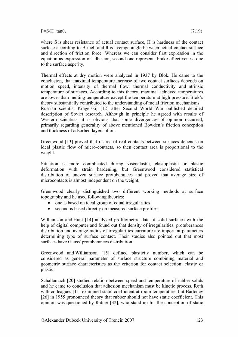
F=S/H+tanθ, (7.19) where S is shear resistance of actual contact surface, H is hardness of the contact surface according to Brinell and θ is average angle between actual contact surface and direction of friction force. Whereas we can consider first expression in the equation as expression of adhesion, second one represents brake effectiveness due to the surface asperity. Thermal effects at dry motion were analyzed in 1937 by Blok. He came to the conclusion, that maximal temperature increase of two contact surfaces depends on motion speed, intensity of thermal flow, thermal conductivity and intrinsic temperature of surfaces. According to this theory, maximal achieved temperatures are lower than melting temperature except the temperature at high pressure. Blok’s theory substantially contributed to the understanding of metal friction mechanisms. Russian scientist Kragelskij [12] after Second World War published detailed description of Soviet research. Although in principle he agreed with results of Western scientists, it is obvious that some divergences of opinion occurred, primarily regarding generality of above mentioned Bowden’s friction conception and thickness of adsorbed layers of oil. Greenwood [13] proved that if area of real contacts between surfaces depends on ideal plastic flow of micro-contacts, so then contact area is proportional to the weight. Situation is more complicated during viscoelastic, elastoplastic or plastic deformation with strain hardening, but Greenwood considered statistical distribution of uneven surface protuberances and proved that average size of microcontacts is almost independent on the weight. Greenwood clearly distinguished two different working methods at surface topography and he used following theories:

• one is based on ideal group of equal irregularities, • second is based directly on measured surface profiles.

Williamson and Hunt [14] analyzed profilometric data of solid surfaces with the help of digital computer and found out that density of irregularities, protuberances distribution and average radius of irregularities curvature are important parameters determining type of surface contact. Their studies also pointed out that most surfaces have Gauss' protuberances distribution. Greenwood and Williamson [15] defined plasticity number, which can be considered as general parameter of surface structure combining material and geometric surface characteristics as the criterion for contact selection: elastic or plastic. Schallamach [20] studied relation between speed and temperature of rubber solids and he came to conclusion that adhesion mechanism must be kinetic process. Roth with colleagues [11] examined static coefficient at room temperature, but Bartenev [26] in 1955 pronounced theory that rubber should not have static coefficient. This opinion was questioned by Ratner [32], who stand up for the conception of static


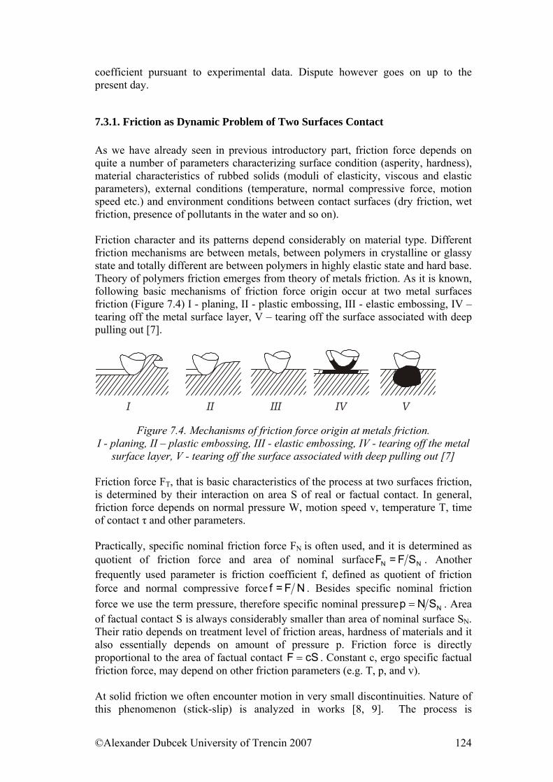
coefficient pursuant to experimental data. Dispute however goes on up to the present day.

7.3.1. Friction as Dynamic Problem of Two Surfaces Contact As we have already seen in previous introductory part, friction force depends on quite a number of parameters characterizing surface condition (asperity, hardness), material characteristics of rubbed solids (moduli of elasticity, viscous and elastic parameters), external conditions (temperature, normal compressive force, motion speed etc.) and environment conditions between contact surfaces (dry friction, wet friction, presence of pollutants in the water and so on). Friction character and its patterns depend considerably on material type. Different friction mechanisms are between metals, between polymers in crystalline or glassy state and totally different are between polymers in highly elastic state and hard base. Theory of polymers friction emerges from theory of metals friction. As it is known, following basic mechanisms of friction force origin occur at two metal surfaces friction (Figure 7.4) I - planing, II - plastic embossing, III - elastic embossing, IV – tearing off the metal surface layer, V – tearing off the surface associated with deep pulling out [7].

I II III IV V

Figure 7.4. Mechanisms of friction force origin at metals friction. I - planing, II – plastic embossing, III - elastic embossing, IV - tearing off the metal

surface layer, V - tearing off the surface associated with deep pulling out [7] Friction force FT, that is basic characteristics of the process at two surfaces friction, is determined by their interaction on area S of real or factual contact. In general, friction force depends on normal pressure W, motion speed v, temperature T, time of contact τ and other parameters. Practically, specific nominal friction force FN is often used, and it is determined as quotient of friction force and area of nominal surface NN SF=F . Another frequently used parameter is friction coefficient f, defined as quotient of friction force and normal compressive force NF=f . Besides specific nominal friction force we use the term pressure, therefore specific nominal pressure NSNp = . Area of factual contact S is always considerably smaller than area of nominal surface SN. Their ratio depends on treatment level of friction areas, hardness of materials and it also essentially depends on amount of pressure p. Friction force is directly proportional to the area of factual contact cSF = . Constant c, ergo specific factual friction force, may depend on other friction parameters (e.g. T, p, and v). At solid friction we often encounter motion in very small discontinuities. Nature of this phenomenon (stick-slip) is analyzed in works [8, 9]. The process is


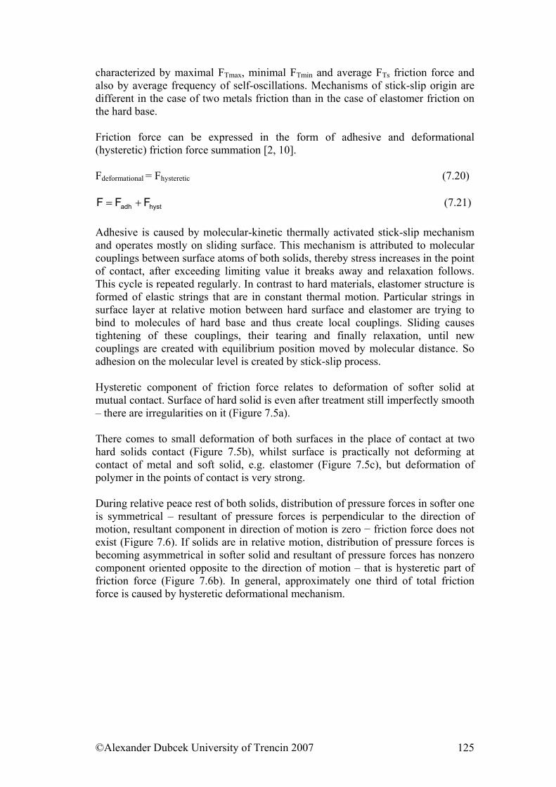
characterized by maximal FTmax, minimal FTmin and average FTs friction force and also by average frequency of self-oscillations. Mechanisms of stick-slip origin are different in the case of two metals friction than in the case of elastomer friction on the hard base. Friction force can be expressed in the form of adhesive and deformational (hysteretic) friction force summation [2, 10]. Fdeformational = Fhysteretic (7.20)

hystadh FFF += (7.21) Adhesive is caused by molecular-kinetic thermally activated stick-slip mechanism and operates mostly on sliding surface. This mechanism is attributed to molecular couplings between surface atoms of both solids, thereby stress increases in the point of contact, after exceeding limiting value it breaks away and relaxation follows. This cycle is repeated regularly. In contrast to hard materials, elastomer structure is formed of elastic strings that are in constant thermal motion. Particular strings in surface layer at relative motion between hard surface and elastomer are trying to bind to molecules of hard base and thus create local couplings. Sliding causes tightening of these couplings, their tearing and finally relaxation, until new couplings are created with equilibrium position moved by molecular distance. So adhesion on the molecular level is created by stick-slip process. Hysteretic component of friction force relates to deformation of softer solid at mutual contact. Surface of hard solid is even after treatment still imperfectly smooth – there are irregularities on it (Figure 7.5a). There comes to small deformation of both surfaces in the place of contact at two hard solids contact (Figure 7.5b), whilst surface is practically not deforming at contact of metal and soft solid, e.g. elastomer (Figure 7.5c), but deformation of polymer in the points of contact is very strong. During relative peace rest of both solids, distribution of pressure forces in softer one is symmetrical – resultant of pressure forces is perpendicular to the direction of motion, resultant component in direction of motion is zero − friction force does not exist (Figure 7.6). If solids are in relative motion, distribution of pressure forces is becoming asymmetrical in softer solid and resultant of pressure forces has nonzero component oriented opposite to the direction of motion – that is hysteretic part of friction force (Figure 7.6b). In general, approximately one third of total friction force is caused by hysteretic deformational mechanism.


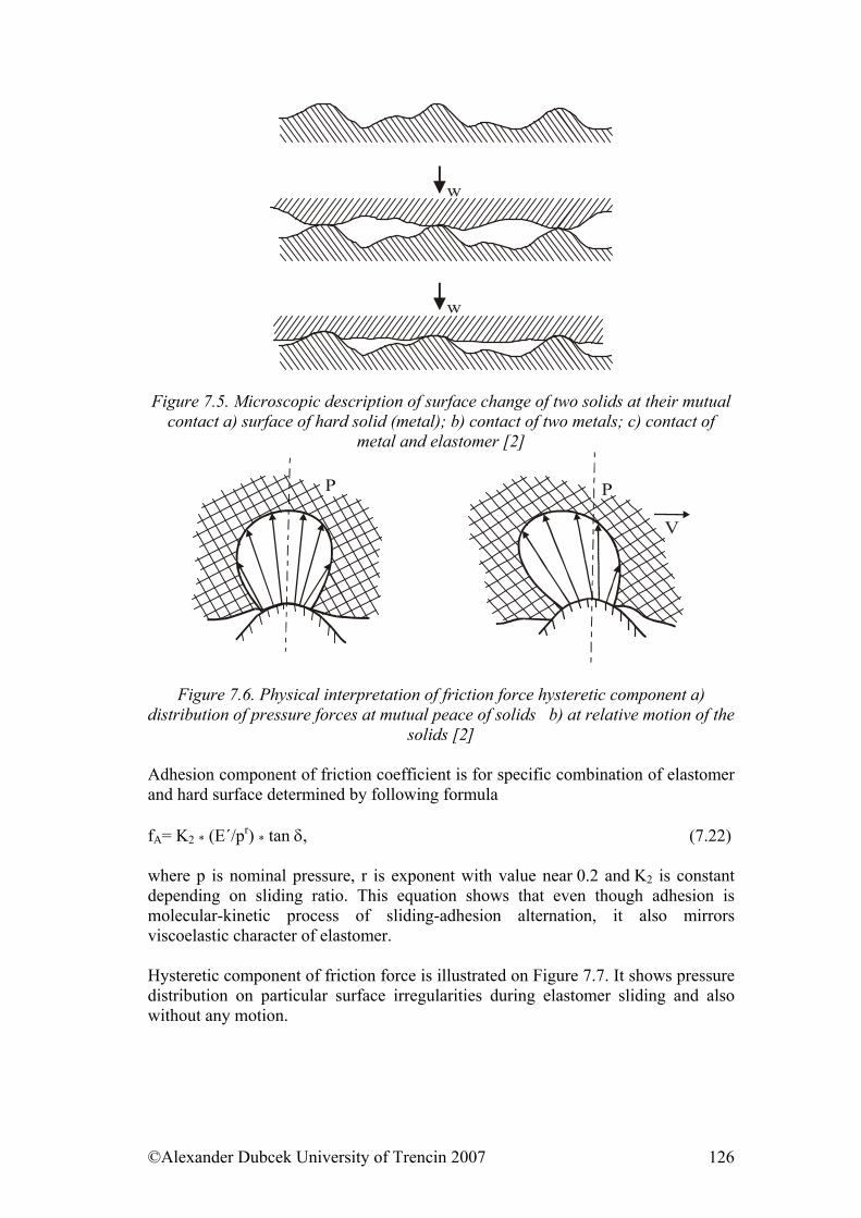
w

w

Figure 7.5. Microscopic description of surface change of two solids at their mutual

contact a) surface of hard solid (metal); b) contact of two metals; c) contact of metal and elastomer [2]

P P

V

Figure 7.6. Physical interpretation of friction force hysteretic component a) distribution of pressure forces at mutual peace of solids b) at relative motion of the

solids [2] Adhesion component of friction coefficient is for specific combination of elastomer and hard surface determined by following formula fA= K2 * (E´/pr) * tan δ, (7.22) where p is nominal pressure, r is exponent with value near 0.2 and K2 is constant depending on sliding ratio. This equation shows that even though adhesion is molecular-kinetic process of sliding-adhesion alternation, it also mirrors viscoelastic character of elastomer. Hysteretic component of friction force is illustrated on Figure 7.7. It shows pressure distribution on particular surface irregularities during elastomer sliding and also without any motion.


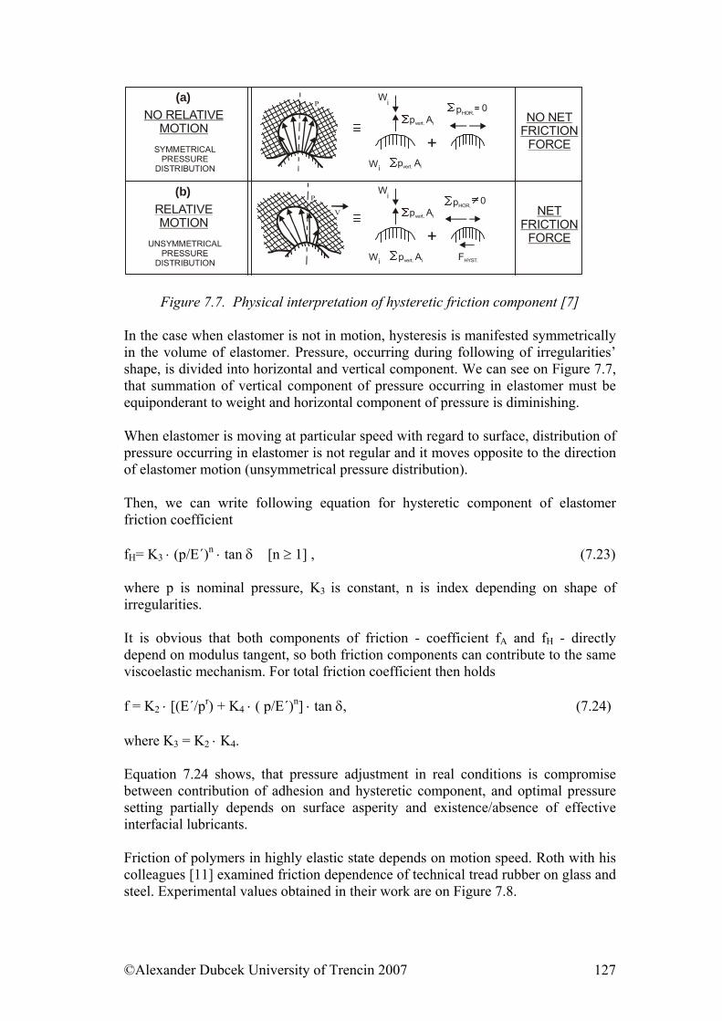
P

P

V

pvert. i A

W

W

i

i

0

+NO NET

FRICTIONFORCE

NETFRICTION

FORCE

W

W

i

i

0

+FHYST.

(b)RELATIVEMOTION

UNSYMMETRICALPRESSURE

DISTRIBUTION

(a)NO RELATIVE

MOTIONSYMMETRICAL

PRESSUREDISTRIBUTION pvert. i A

pHOR.

pHOR.

pvert. i A

pvert. i A

Figure 7.7. Physical interpretation of hysteretic friction component [7] In the case when elastomer is not in motion, hysteresis is manifested symmetrically in the volume of elastomer. Pressure, occurring during following of irregularities’ shape, is divided into horizontal and vertical component. We can see on Figure 7.7, that summation of vertical component of pressure occurring in elastomer must be equiponderant to weight and horizontal component of pressure is diminishing. When elastomer is moving at particular speed with regard to surface, distribution of pressure occurring in elastomer is not regular and it moves opposite to the direction of elastomer motion (unsymmetrical pressure distribution). Then, we can write following equation for hysteretic component of elastomer friction coefficient fH= K3 ⋅ (p/E´)n ⋅ tan δ [n ≥ 1] , (7.23) where p is nominal pressure, K3 is constant, n is index depending on shape of irregularities. It is obvious that both components of friction - coefficient fA and fH - directly depend on modulus tangent, so both friction components can contribute to the same viscoelastic mechanism. For total friction coefficient then holds f = K2 ⋅ [(E´/pr) + K4 ⋅ ( p/E´)n] ⋅ tan δ, (7.24) where K3 = K2 ⋅ K4. Equation 7.24 shows, that pressure adjustment in real conditions is compromise between contribution of adhesion and hysteretic component, and optimal pressure setting partially depends on surface asperity and existence/absence of effective interfacial lubricants. Friction of polymers in highly elastic state depends on motion speed. Roth with his colleagues [11] examined friction dependence of technical tread rubber on glass and steel. Experimental values obtained in their work are on Figure 7.8.


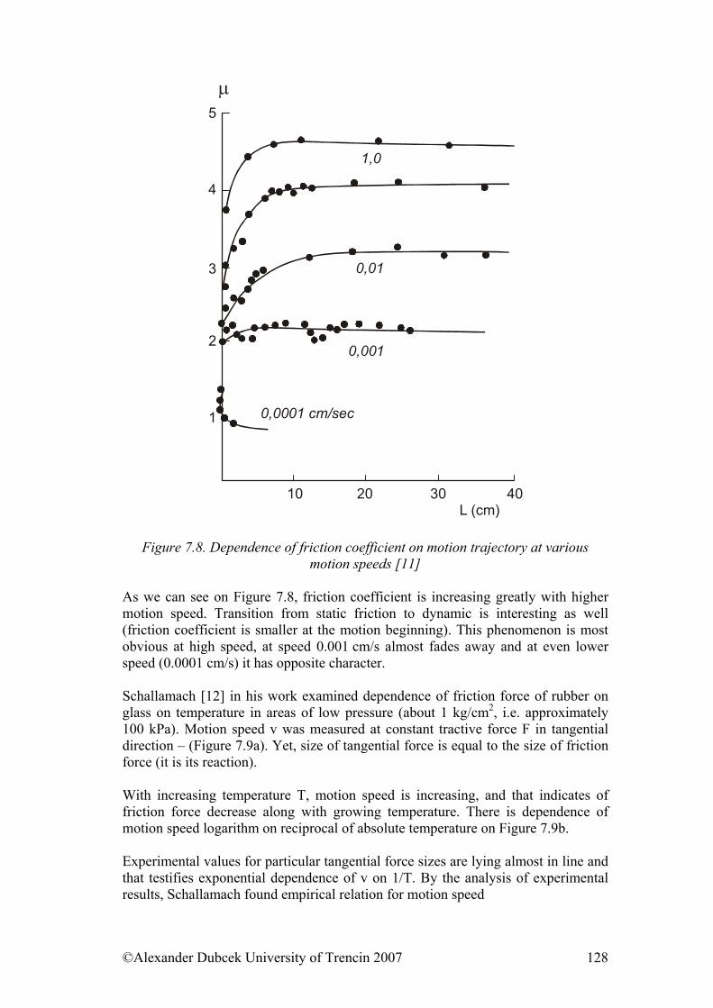
µ

3

10 20 30 40

1

2

4

5

1,0

0,01

0,001

0,0001 cm/sec

L (cm)

Figure 7.8. Dependence of friction coefficient on motion trajectory at various motion speeds [11]

As we can see on Figure 7.8, friction coefficient is increasing greatly with higher motion speed. Transition from static friction to dynamic is interesting as well (friction coefficient is smaller at the motion beginning). This phenomenon is most obvious at high speed, at speed 0.001 cm/s almost fades away and at even lower speed (0.0001 cm/s) it has opposite character. Schallamach [12] in his work examined dependence of friction force of rubber on glass on temperature in areas of low pressure (about 1 kg/cm2, i.e. approximately 100 kPa). Motion speed v was measured at constant tractive force F in tangential direction – (Figure 7.9a). Yet, size of tangential force is equal to the size of friction force (it is its reaction). With increasing temperature T, motion speed is increasing, and that indicates of friction force decrease along with growing temperature. There is dependence of motion speed logarithm on reciprocal of absolute temperature on Figure 7.9b. Experimental values for particular tangential force sizes are lying almost in line and that testifies exponential dependence of v on 1/T. By the analysis of experimental results, Schallamach found empirical relation for motion speed


⎟⎠⎞

⎜⎝⎛=

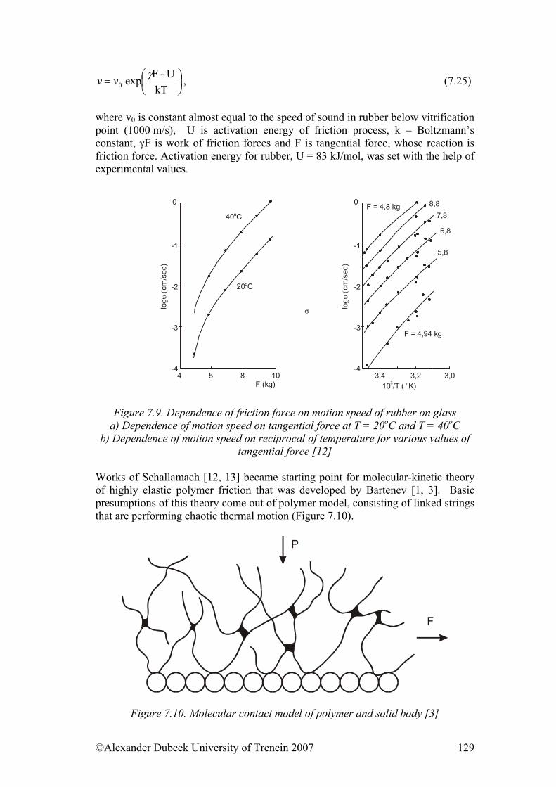
kTU-Fexp0

γvv , (7.25)

where v0 is constant almost equal to the speed of sound in rubber below vitrification point (1000 m/s), U is activation energy of friction process, k – Boltzmann’s constant, γF is work of friction forces and F is tangential force, whose reaction is friction force. Activation energy for rubber, U = 83 kJ/mol, was set with the help of experimental values.

-1

-3

-2

54 8 10-4

40 CO

20 CO

-1

-3

-2

3,410 /T ( K)3 O

-43,2 3,0

F = 4,94 kg

F = 4,8 kg 8,87,8

6,8

5,8

00

log

cm/s

ec)

υ (

σ

F (kg)

log

cm/s

ec)

υ (

Figure 7.9. Dependence of friction force on motion speed of rubber on glass

a) Dependence of motion speed on tangential force at T = 20oC and T = 40oC b) Dependence of motion speed on reciprocal of temperature for various values of

tangential force [12] Works of Schallamach [12, 13] became starting point for molecular-kinetic theory of highly elastic polymer friction that was developed by Bartenev [1, 3]. Basic presumptions of this theory come out of polymer model, consisting of linked strings that are performing chaotic thermal motion (Figure 7.10).

F

P

Figure 7.10. Molecular contact model of polymer and solid body [3]


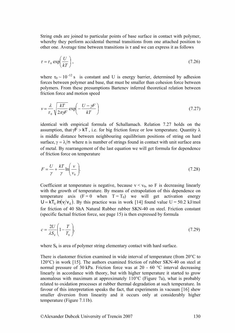
String ends are joined to particular points of base surface in contact with polymer, whereby they perform accidental thermal transitions from one attached position to other one. Average time between transitions is τ and we can express it as follows

⎟⎠⎞

⎜⎝⎛=

kTUexp0ττ , (7.26)

where τ0 ~ 10 -12 s is constant and U is energy barrier, determined by adhesion forces between polymer and base, that must be smaller than cohesion force between polymers. From these presumptions Bartenev inferred theoretical relation between friction force and motion speed

⎟⎠⎞

⎜⎝⎛ −

−=kT

FUF

kTv γπγτ

λ exp20

(7.27)

identical with empirical formula of Schallamach. Relation 7.27 holds on the assumption, that kTF >γ , i.e. for big friction force or low temperature. Quantity λ is middle distance between neighbouring equilibrium positions of string on hard surface, nλ=γ where n is number of strings found in contact with unit surface area of metal. By rearrangement of the last equation we will get formula for dependence of friction force on temperature

⎟⎟⎠

⎞⎜⎜⎝

⎛+=

0

lnvvkTUF

γγ. (7.28)

Coefficient at temperature is negative, because v < v0, so F is decreasing linearly with the growth of temperature. By means of extrapolation of this dependence on temperature axis (F = 0 when T = T0) we will get activation energy

( 00 vvkTU ln= ). By this practice was in work [14] found value U = 50.2 kJ/mol for friction of 40 ShA Natural Rubber rubber SKN-40 on steel. Friction constant (specific factual friction force, see page 15) is then expressed by formula

⎟⎟⎠

⎞⎜⎜⎝

⎛−=

0

12TT

SUc

kλ, (7.29)

where Sk is area of polymer string elementary contact with hard surface. There is elastomer friction examined in wide interval of temperature (from 20°C to 120°C) in work [15]. The authors examined friction of rubber SKN-40 on steel at normal pressure of 30 kPa. Friction force was at 20 - 60 °C interval decreasing linearly in accordance with theory, but with higher temperature it started to grow anomalous with maximum at approximately 110°C (Figure 7a), what is probably related to oxidation processes at rubber thermal degradation at such temperature. In favour of this interpretation speaks the fact, that experiments in vacuum [16] shew smaller diversion from linearity and it occurs only at considerably higher temperature (Figure 7.11b).


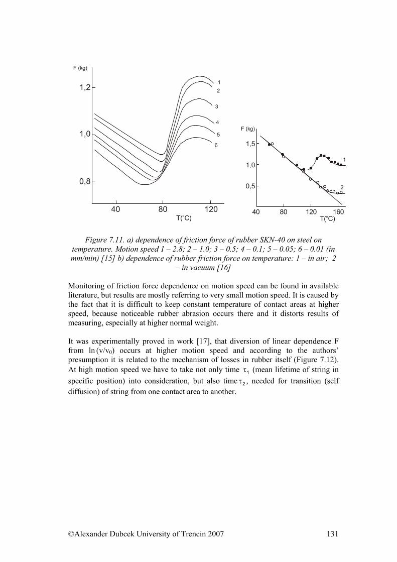
12

3

4

5

6

1,2

1,0

0,8

40 80 120

1

2

1,5

1,0

0,5

40 80 160120

F (kg)

T( C)o T( C)o

F (kg)

Figure 7.11. a) dependence of friction force of rubber SKN-40 on steel on

temperature. Motion speed 1 – 2.8; 2 – 1.0; 3 – 0.5; 4 – 0.1; 5 – 0.05; 6 – 0.01 (in mm/min) [15] b) dependence of rubber friction force on temperature: 1 – in air; 2

– in vacuum [16] Monitoring of friction force dependence on motion speed can be found in available literature, but results are mostly referring to very small motion speed. It is caused by the fact that it is difficult to keep constant temperature of contact areas at higher speed, because noticeable rubber abrasion occurs there and it distorts results of measuring, especially at higher normal weight. It was experimentally proved in work [17], that diversion of linear dependence F from ln (v/v0) occurs at higher motion speed and according to the authors’ presumption it is related to the mechanism of losses in rubber itself (Figure 7.12). At high motion speed we have to take not only time 1τ (mean lifetime of string in specific position) into consideration, but also time 2τ , needed for transition (self diffusion) of string from one contact area to another.


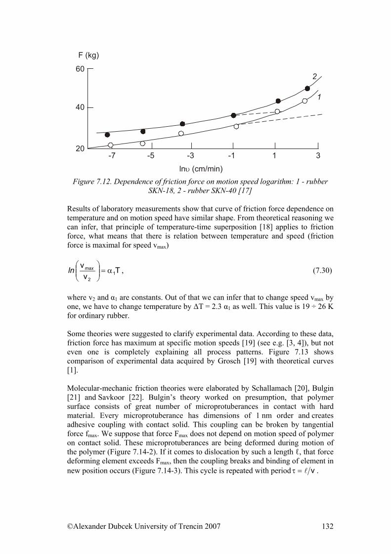
60

40

20-7 -5 -3 -1 1 3

ln (cm/min)υ

F (kg)

2

1

Figure 7.12. Dependence of friction force on motion speed logarithm: 1 - rubber

SKN-18, 2 - rubber SKN-40 [17] Results of laboratory measurements show that curve of friction force dependence on temperature and on motion speed have similar shape. From theoretical reasoning we can infer, that principle of temperature-time superposition [18] applies to friction force, what means that there is relation between temperature and speed (friction force is maximal for speed vmax)

Tv

v1

2

α=⎟⎟⎠

⎞⎜⎜⎝

⎛ maxln , (7.30)

where v2 and α1 are constants. Out of that we can infer that to change speed vmax by one, we have to change temperature by ∆T = 2.3 α1 as well. This value is 19 ÷ 26 K for ordinary rubber. Some theories were suggested to clarify experimental data. According to these data, friction force has maximum at specific motion speeds [19] (see e.g. [3, 4]), but not even one is completely explaining all process patterns. Figure 7.13 shows comparison of experimental data acquired by Grosch [19] with theoretical curves [1]. Molecular-mechanic friction theories were elaborated by Schallamach [20], Bulgin [21] and Savkoor [22]. Bulgin’s theory worked on presumption, that polymer surface consists of great number of microprotuberances in contact with hard material. Every microprotuberance has dimensions of 1 nm order and creates adhesive coupling with contact solid. This coupling can be broken by tangential force fmax. We suppose that force Fmax does not depend on motion speed of polymer on contact solid. These microprotuberances are being deformed during motion of the polymer (Figure 7.14-2). If it comes to dislocation by such a length ℓ, that force deforming element exceeds Fmax, then the coupling breaks and binding of element in new position occurs (Figure 7.14-3). This cycle is repeated with period vl=τ .


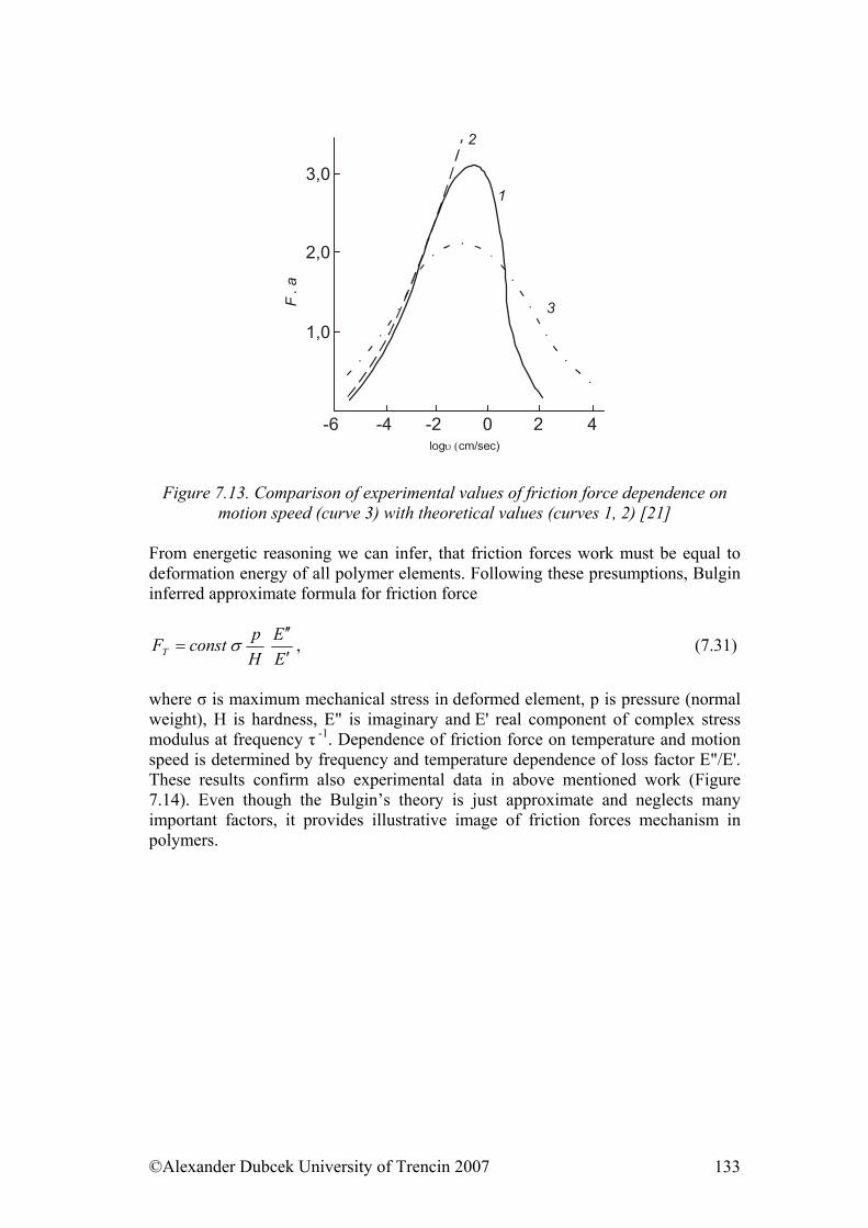
3,0

2,0

1,0

-6 -4 -2 0 2 4

2

1

3F . a

log cm/sec)υ (

Figure 7.13. Comparison of experimental values of friction force dependence on

motion speed (curve 3) with theoretical values (curves 1, 2) [21] From energetic reasoning we can infer, that friction forces work must be equal to deformation energy of all polymer elements. Following these presumptions, Bulgin inferred approximate formula for friction force

EE

HpconstFT ′

′′= σ , (7.31)

where σ is maximum mechanical stress in deformed element, p is pressure (normal weight), H is hardness, E" is imaginary and E' real component of complex stress modulus at frequency τ -1. Dependence of friction force on temperature and motion speed is determined by frequency and temperature dependence of loss factor E"/E'. These results confirm also experimental data in above mentioned work (Figure 7.14). Even though the Bulgin’s theory is just approximate and neglects many important factors, it provides illustrative image of friction forces mechanism in polymers.


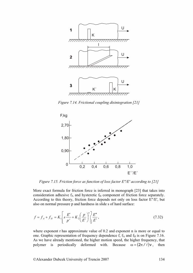
K´ K

U

U

U

K

l

Figure 7.14. Frictional coupling disintegration [21]

F,kg

E´´/E´0,2 0,60,4 0,8 1,0

2,70

1,80

0,90

0

Figure 7.15. Friction force as function of loss factor E"/E' according to [21] More exact formula for friction force is inferred in monograph [23] that takes into consideration adhesive fA and hysteretic fH component of friction force separately. According to this theory, friction force depends not only on loss factor E"/E', but also on normal pressure p and hardness in slide s of hard surface:

EE

EpK

pEsKfff

n

rHA ′′′

⎥⎥⎦

⎤

⎢⎢⎣

⎡⎟⎠⎞

⎜⎝⎛

′+

′=+= 21 , (7.32)

where exponent r has approximate value of 0.2 and exponent n is more or equal to one. Graphic representation of frequency dependence f, fA and fH is on Figure 7.16. As we have already mentioned, the higher motion speed, the higher frequency, that polymer is periodically deformed with. Because ( )v2 l/π=ω , then


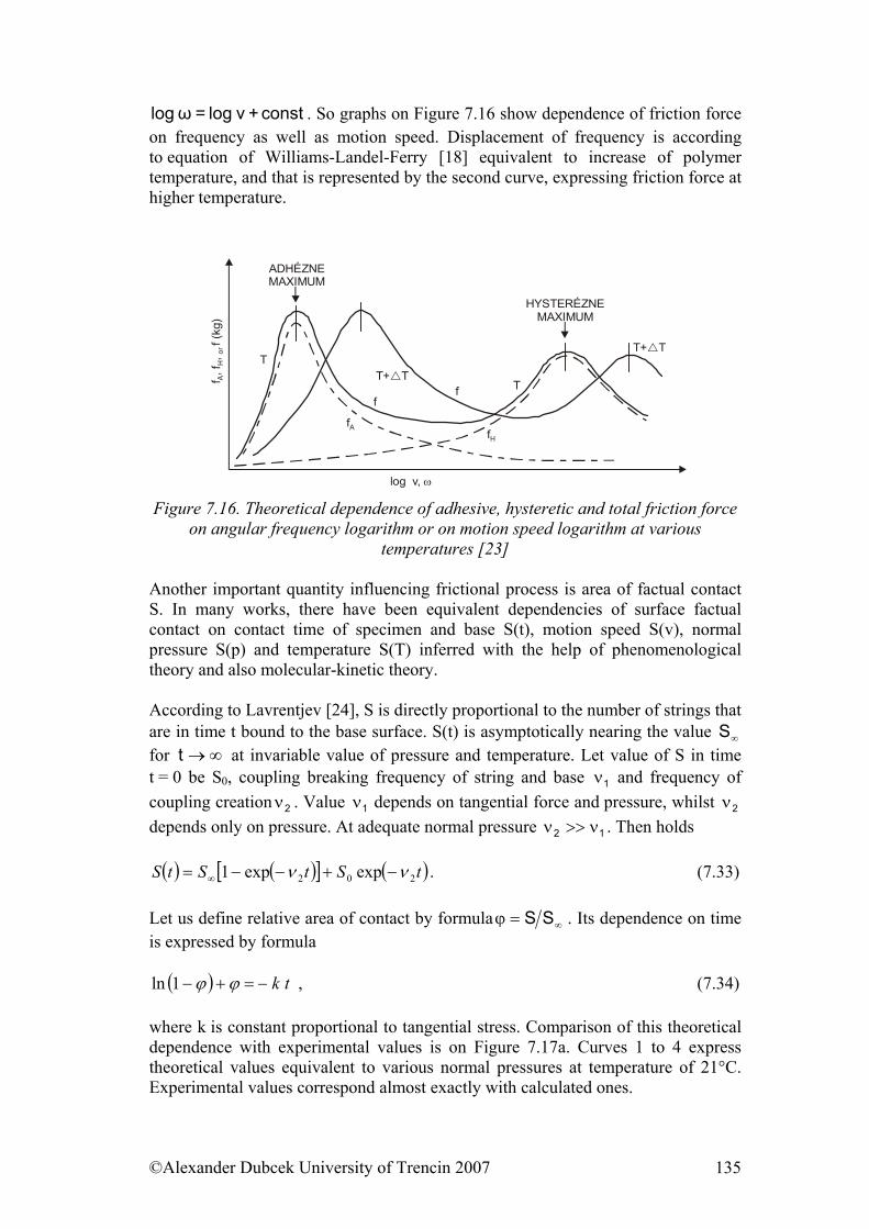
const+vlog=ωlog . So graphs on Figure 7.16 show dependence of friction force on frequency as well as motion speed. Displacement of frequency is according to equation of Williams-Landel-Ferry [18] equivalent to increase of polymer temperature, and that is represented by the second curve, expressing friction force at higher temperature.

T+ T

T+ T

ADHÉZNEMAXIMUM

HYSTERÉZNEMAXIMUM

T

fHfA

ff

T

f, f

, f (

kg)

AH

or

log v, ω

Figure 7.16. Theoretical dependence of adhesive, hysteretic and total friction force on angular frequency logarithm or on motion speed logarithm at various

temperatures [23] Another important quantity influencing frictional process is area of factual contact S. In many works, there have been equivalent dependencies of surface factual contact on contact time of specimen and base S(t), motion speed S(v), normal pressure S(p) and temperature S(T) inferred with the help of phenomenological theory and also molecular-kinetic theory. According to Lavrentjev [24], S is directly proportional to the number of strings that are in time t bound to the base surface. S(t) is asymptotically nearing the value for at invariable value of pressure and temperature. Let value of S in time t = 0 be S

∞S∞→t

0, coupling breaking frequency of string and base 1ν and frequency of coupling creation . Value depends on tangential force and pressure, whilst 2ν 1ν 2ν depends only on pressure. At adequate normal pressure 12 ν>>ν . Then holds

( ) ( )[ ] ( )tStStS 202 expexp1 νν −+−−= ∞ . (7.33) Let us define relative area of contact by formula ∞=ϕ SS . Its dependence on time is expressed by formula

( ) tk−=+− ϕϕ1ln , (7.34) where k is constant proportional to tangential stress. Comparison of this theoretical dependence with experimental values is on Figure 7.17a. Curves 1 to 4 express theoretical values equivalent to various normal pressures at temperature of 21°C. Experimental values correspond almost exactly with calculated ones.


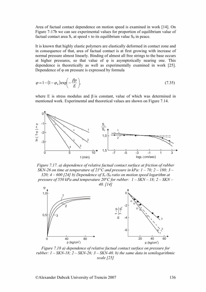
Area of factual contact dependence on motion speed is examined in work [14]. On Figure 7-17b we can see experimental values for proportion of equilibrium value of factual contact area Sv at speed v to its equilibrium value S0 in peace. It is known that highly elastic polymers are elastically deformed in contact zone and in consequence of that, area of factual contact is at first growing with increase of normal pressure almost linearly. Binding of almost all free strings to the base occurs at higher pressures, so that value of φ is asymptotically nearing one. This dependence is theoretically as well as experimentally examined in work [25]. Dependence of φ on pressure is expressed by formula

( ) ⎟⎠⎞

⎜⎝⎛−−−=

Epβϕϕ exp11 0 , (7.35)

where E is stress modulus and β is constant, value of which was determined in mentioned work. Experimental and theoretical values are shown on Figure 7.14.

1

2

34

0

-3

-2

-1

ln (

1- )

+ ϕ

ϕ

5 100

S0

Sυ

1,5-7 -5 -3 -1 1 3

1,0

1

2

t (min) log cm/sec)υ (

Figure 7.17. a) dependence of relative factual contact surface at friction of rubber SKN-26 on time at temperature of 21°C and pressure in kPa: 1 – 70; 2 – 180; 3 –

320; 4 – 600 [24] b) Dependence of Sv /S0 ratio on motion speed logarithm at pressure of 550 kPa and temperature 20°C for rubber: 1 – SKN – 18; 2 – SKN –

40. [14]

1,0

0,5

0 40 80

1

2

3

ϕ

20 40 60

0

-4

-6

-2

3

2

1

ln1

- ϕ1

- ϕ0

p (kg/cm )2p (kg/cm )2

Figure 7.18 a) dependence of relative factual contact surface on pressure for

rubber: 1 – SKN-18; 2 – SKN-26; 3 – SKN-40. b) the same data in semilogarithmic scale [25]


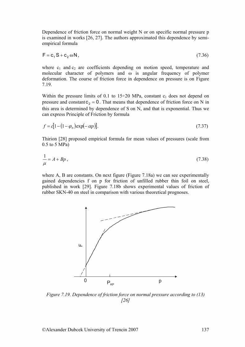
Dependence of friction force on normal weight N or on specific normal pressure p is examined in works [26, 27]. The authors approximated this dependence by semi-empirical formula

NcScF 21 ω+= , (7.36) where c1 and c2 are coefficients depending on motion speed, temperature and molecular character of polymers and ω is angular frequency of polymer deformation. The course of friction force in dependence on pressure is on Figure 7.19. Within the pressure limits of 0.1 to 15÷20 MPa, constant c1 does not depend on pressure and constant . That means that dependence of friction force on N in this area is determined by dependence of S on N, and that is exponential. Thus we can express Principle of Friction by formula

0c2 =

( ) ([ pcf )]αϕ −−−= exp11 0 . (7.37)

Thirion [28] proposed empirical formula for mean values of pressures (scale from 0.5 to 5 MPa)

BpA +=µ1 , (7.38)

where A, B are constants. On next figure (Figure 7.18a) we can see experimentally gained dependencies f on p for friction of unfilled rubber thin foil on steel, published in work [29]. Figure 7.18b shows experimental values of friction of rubber SKN-40 on steel in comparison with various theoretical prognoses.

F

0 pPKP

Figure 7.19. Dependence of friction force on normal pressure according to (13) [26]


13

2

400 800 1200

75

45

30

15

60

400 600 10001000 1400

140

100

20

60

180

p (kg/cm )2p (kg/cm )2

f (kg

/cm

)2

f (kg

/cm

)2

Figure 7.20. a) dependence of specific friction force on pressure for friction of unfilled rubber thin foil on steel. According to [29]. b) dependence of specific friction force on pressure for rubber SKN-40 on steel: 1 – experiment, 2 – low

pressure theory, 3 – high pressure theory [26] Wet friction is complicated process, when there is thin film of liquid material – water, oil and the like – of variable thickness between surface of elastomer and hard solid (Figure 7.21). Providing that there is constant viscosity µ (for friction) η (for viscosity) and density ρ of liquid film, we can write equation for its motion

( ) ( )th

uuhxh

uuyp

hyx

ph

x ∂∂

+++∂∂

−=⎥⎦

⎤⎢⎣

⎡∂∂

∂∂

+⎥⎦

⎤⎢⎣

⎡∂∂

∂∂ µµµ 1266 2121

33 , (7.39)

where u1 and u2 are speeds of upper and lower surface of rubbed solids, p is hydrodynamic pressure. In the case, that one of the solids is elastomer, situation expressed on Figure 7.22 occurs. Elastomer is deformed on hard base protuberances and liquid film is divided into specific parts where areas of increased and reduced pressure alternate. Such a friction mechanism is analyzed in works [23, 30].

h

u2

u1V =

dhdt

z,h

x

y

ρ, µ, p

Figure 7.21. Contact of two solids separated by a film of liquid. According to [2] Resultant friction force greatly depends on surface relief (microscopic irregularities, macroscopic irregularities), motion speed, temperature, pressure and liquid film parameters. Theoretical description in full extent does not exist. There are only some empirical formulas for specific cases and many experimental data.


+ + +--

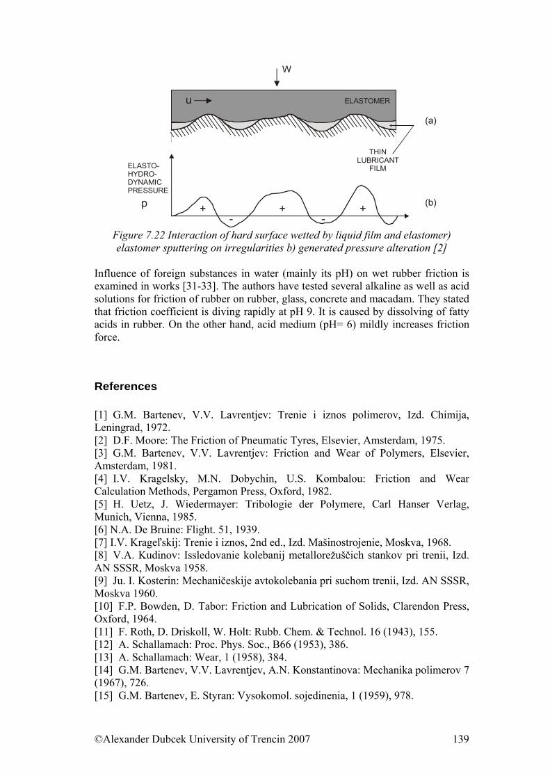
W

THINLUBRICANT

FILMELASTO-HYDRO-DYNAMICPRESSURE

(b)

(a)

p

ELASTOMERu

Figure 7.22 Interaction of hard surface wetted by liquid film and elastomer) elastomer sputtering on irregularities b) generated pressure alteration [2]

Influence of foreign substances in water (mainly its pH) on wet rubber friction is examined in works [31-33]. The authors have tested several alkaline as well as acid solutions for friction of rubber on rubber, glass, concrete and macadam. They stated that friction coefficient is diving rapidly at pH 9. It is caused by dissolving of fatty acids in rubber. On the other hand, acid medium (pH= 6) mildly increases friction force.

References [1] G.M. Bartenev, V.V. Lavrentjev: Trenie i iznos polimerov, Izd. Chimija, Leningrad, 1972. [2] D.F. Moore: The Friction of Pneumatic Tyres, Elsevier, Amsterdam, 1975. [3] G.M. Bartenev, V.V. Lavrentjev: Friction and Wear of Polymers, Elsevier, Amsterdam, 1981. [4] I.V. Kragelsky, M.N. Dobychin, U.S. Kombalou: Friction and Wear Calculation Methods, Pergamon Press, Oxford, 1982. [5] H. Uetz, J. Wiedermayer: Tribologie der Polymere, Carl Hanser Verlag, Munich, Vienna, 1985. [6] N.A. De Bruine: Flight. 51, 1939. [7] I.V. Krageľskij: Trenie i iznos, 2nd ed., Izd. Mašinostrojenie, Moskva, 1968. [8] V.A. Kudinov: Issledovanie kolebanij metallorežuščich stankov pri trenii, Izd. AN SSSR, Moskva 1958. [9] Ju. I. Kosterin: Mechaničeskije avtokolebania pri suchom trenii, Izd. AN SSSR, Moskva 1960. [10] F.P. Bowden, D. Tabor: Friction and Lubrication of Solids, Clarendon Press, Oxford, 1964. [11] F. Roth, D. Driskoll, W. Holt: Rubb. Chem. & Technol. 16 (1943), 155. [12] A. Schallamach: Proc. Phys. Soc., B66 (1953), 386. [13] A. Schallamach: Wear, 1 (1958), 384. [14] G.M. Bartenev, V.V. Lavrentjev, A.N. Konstantinova: Mechanika polimerov 7 (1967), 726. [15] G.M. Bartenev, E. Styran: Vysokomol. sojedinenia, 1 (1959), 978.


[16] A.I. Jelkin, V.N. Nikolejev: DAN SSSR, 173 (1967), 1302. [17] G.M. Bartenev, V.V. Lavrentjev, N.A. Konstantinova: Mechanika polimerov 3 (1967), 309. [18] M.L. Williams, R.F.Landel, J.D.Ferry: J. Amer. Chem. Soc., 77 (1955), 3107. [19] K. Grosch, Proc. Roy. Soc. 247A (1963), 21. [20] A. Schallamach: Wear, 6 (1963). [21] D. Bulgin: Rubb. Plast. Weekly, 143 (1962), 636. [22] A. Savkoor: Wear, 8 (1965), 221. [23] D.F. Moore: The Friction and Lubrication of Elastomers, Pergamon Press, Oxford, 1972. [24] V.V. Lavrentjev: DAN SSSR, 175, 1 (1967). [25] N.A. Konstantinova: Dizertačná práca, MGPI, Moskva 1967. [26] G.M. Bartenev: DAN SSSR, 103, (1955), 1017. [27] J. Slabeycius: Internal Report for Matador, Puchov, 2000. [28] P. Thirion: Rubb. Chem. and Technology, 21 (1948), 505. [29] B.V. Derjagin, Yu.P. Toporov: DAN SSSR, 146, (1962), 1356. [30] J. Hirama, H. Ishiwata: Paper No.15, Proc. Inst. Mech. Eng., 180 (1965/66), 187. [31] A.D. Roberts: Rubb. Develop. 49 (1996), 18. [32] A.D. Roberts, S.C. Richards: Gummi Fasern Kunststoffe 50 (1997), 978. [33] A.D. Roberts, S.C. Richards: Rubb. Develop. 49 (1996), 54. Fundamental questions from presented part 1. What is the origin of polymers hysteresis? 2. What factors determine the firmness of glued joints? 3. Define the surface tension. 4. What type of tread surface yields the maximal adhesion on the wet and on the dry road? 5. Describe the stick-slip process in the case of elastomer friction on the hard base.


Documents

LEXANDER UBCEK NIVERSITY OF RENCIN